Scope & Usage
Scope
SMAP haplotype-sites: using polymorphic sites (SNPs, SVs, and/or SMAPs) for read-backed haplotyping
SMAP haplotype-sites only requires this input:
a single BED file to define the start and end points of loci (loci created by SMAP delineate for GBS, amplicon regions for HiPlex, and Sliding frames for Shotgun sequencing).
a single VCF file containing bi-allelic SNPs obtained with third-party SNP calling software.
a set of indexed BAM files for all samples that need to be compared.
Loci with sets of polymorphic sites
Integration in the SMAP workflow
SMAP haplotype-sites is run on a set of BAM files, using BED files with locus positions created by SMAP delineate, SMAP sliding-frames or SMAP design, and a VCF file with SNP variants obtained with third-party software. Genotype call tables created by SMAP haplotype-sites may further be analysed with SMAP relatednes. SMAP haplotype-sites works on GBS, HiPlex and Shotgun sequencing data.
Required input
Depending on the type of data (HiPlex, Shotgun, or GBS), a specific BED file must be created to define the start and end positions of loci.
Typical Primer3 output that needs to be converted to a BED file to delineate the loci for SMAP haplotype-sites.
Index
Seq ID
Count
Primer_type
Orientation
Start
Len
tm
GC%
Any compl
3’ compl
Seq
Prod Size
Seq Length
Included Length
Pair any compl
Pair 3’ compl
1
Chr1
1
Generic
FORWARD
2
16
58.72
56.25
5.00
0.00
ATTCTCCGGGGTCACT
72
29887145
29887145
6.00
3.00
2
Chr1
1
Generic
REVERSE
73
17
59.69
47.05
4.00
2.00
GTACACCGGTATTCTTC
3
Chr1
1
Generic
FORWARD
92
20
59.65
45.00
3.00
3.00
CCCAAAAATCCCAGTGACAT
83
29887145
29887145
3.00
1.00
4
Chr1
1
Generic
REVERSE
174
20
58.88
55.00
3.00
0.00
TGACAGTAGCCCAAGAGGTG
5
Chr1
1
Generic
FORWARD
294
20
60.01
60.00
4.00
0.00
GCTAGTGGGAGCTGAAGTGG
81
29887145
29887145
3.00
1.00
6
Chr1
1
Generic
REVERSE
374
20
60.28
50.00
4.00
2.00
TAGTGCTGGCAACGACCATA
7
Chr1
1
Generic
FORWARD
463
20
60.79
60.00
6.00
0.00
GCTGCAGGGTAAGGAGAGGT
84
29887145
29887145
5.00
1.00
8
Chr1
1
Generic
REVERSE
546
21
59.00
47.62
8.00
2.00
GGATATCCTTGTCGAACTCCA
The scheme below outlines the relative positions of primers and loci on the reference genome sequence.
For HiPlex data, the user needs to create a custom BED file listing the loci based on the primer binding sites. We recommend to keep primer sequences in HiPlex reads for mapping, but to define the region between the primers in the BED file used for SMAP haplotype-sites. This region is defined by the first nucleotide downstream of the forward primer binding site to the last nucleotide upstream of the reverse primer binding site.
The primer binding site coordinates (using GFF coordinate system for primers: start and end both 1-based) need to be transformed as follows:
BED
INPUT
Reference
reference sequence ID
Start
F-primer end position (F-primer end given as 1-based coordinate)
End
R-primer start position - 1 (R-primer start given as 1-based coordinate)
HiPlex_locus_name
reference_(F-primer end position + 1)_(R-primer start position - 1)
Mean_Read_Depth
.
Strand
+
SMAPs
(F-primer end position + 1), (R-primer start position - 1)
Completeness
.
nr_SMAPs
2
Name
HiPlex_Set1
The table below corresponds to the four loci defined by the Primer3 output shown above.
Reference
Start
End
HiPlex_locus_name
Mean_read_depth
Strand
SMAPs
Completeness
nr_SMAPs
Name
Chr1
17
56
Chr1:18-56_+
.
+
18,56
.
2
HiPlex_Set1
Chr1
111
164
Chr1:112-164_+
.
+
112,164
.
2
HiPlex_Set1
Chr1
313
354
Chr1:314-354_+
.
+
314,354
.
2
HiPlex_Set1
Chr1
482
525
Chr1:483-525_+
.
+
483,525
.
2
HiPlex_Set1
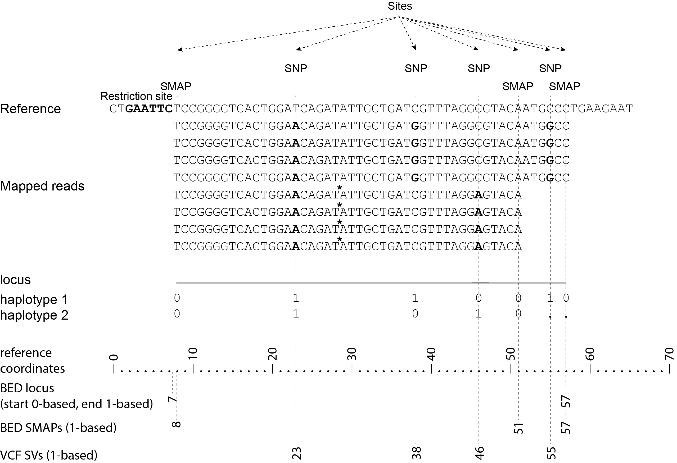
Consider the following read mapping and associated VCF file with several neighboring SNPs.
The user needs to create a custom BED file listing the loci based on a VCF file with SNPs. Sliding frames are created starting from the first SNP in the sequence, We recommend to define 3bp Sliding frames with the central nucleotide at the junction and two flanking nucleotides as SMAPs in the BED file used for SMAP haplotype-sites. Each junction on both ends of a structural variant may be genotyped independently.
Reference
Start
End
HiPlex_locus_name
Mean_read_depth
Strand
SMAPs
Completeness
nr_SMAPs
Name
Chr1
16
32
Chr1:17-32_+
.
+
17,32
.
2
HiPlex_Set1
Chr1
39
56
Chr1:40-56_+
.
+
40,56
.
2
HiPlex_Set1
Chr1
107
108
Chr1:108-108_+
.
+
108,108
.
2
HiPlex_Set1
The SNP coordinates need to be transformed into sliding frames as follows:
BED
INPUT
Reference
reference sequence ID
Start
first SNP position in frame - offset - 1
End
last SNP position in frame + offset
Shotgun_locus_name
reference_start_end
Mean_Read_Depth
.
Strand
+
SMAPs
First SNP position - offset, last SNP position + Offset
Completeness
.
nr_SMAPs
2
Name
Shotgun_Set1
Consider the following read mapping structure and associated VCF file with structural variants.
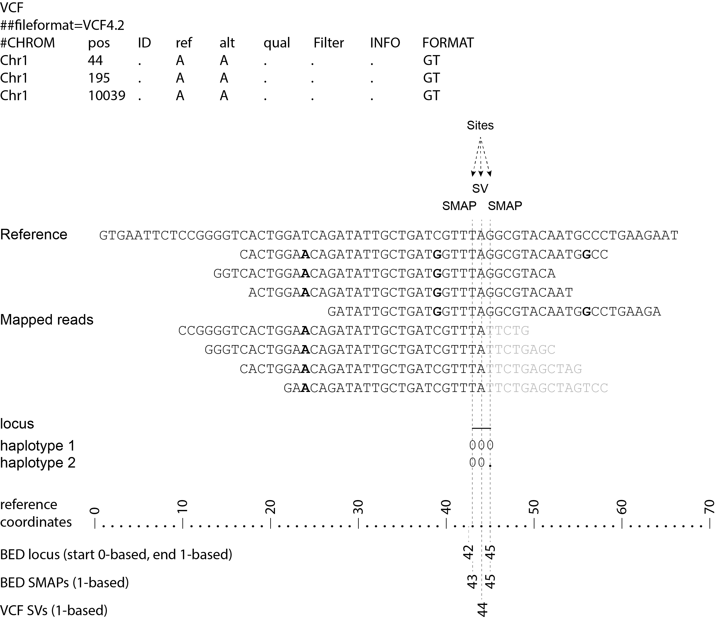
The user needs to create a custom BED file listing the loci based on a VCF file with known junctions of Stuctural Variants. We recommend to define 3bp Sliding frames with the central nucleotide at the junction and two flanking nucleotides as SMAPs in the BED file used for SMAP haplotype-sites. Each junction on both ends of a structural variant may be genotyped independently.
Reference
Start
End
HiPlex_locus_name
Mean_read_depth
Strand
SMAPs
Completeness
nr_SMAPs
Name
Chr1
42
45
Chr1:43-45_+
.
+
43,45
.
2
Shotgun_Set2
Chr1
193
196
Chr1:194-196_+
.
+
194,196
.
2
Shotgun_Set2
Chr1
10038
10041
Chr1:10039-10041_+
.
+
10039,10041
.
2
Shotgun_Set2
The SV coordinates need to be transformed to short Sliding frames as follows:
BED
INPUT
Reference
reference sequence ID
Start
SV position - 2
End
SV position + 1
Shotgun_locus_name
reference_(SV position - 1)_(SV position + 1)
Mean_Read_Depth
.
Strand
+
SMAPs
(SV position - 1), (SV position + 1)
Completeness
.
nr_SMAPs
2
Name
Shotgun_Set2
For GBS data, the user needs to run SMAP delineate on the same set of BAM files as will be used for haplotyping to create a BED file listing the loci with SMAPs. The read mapping profiles determine the locus start and end points and internal SMAPs.
Reference
Start
End
MergedCluster_name
Mean_read_depth
Strand
SMAPs
Completeness
nr_SMAPs
Name
scaffold_10030
15617
15711
scaffold_10030:15618-15711_+
1899
+
15618,15622,15703,15711
13
4
2n_ind_GBS_SE
scaffold_10030
15712
15798
“scaffold_10030:15713-15798_-”
1930
-
15713,15793,15798
9
3
2n_ind_GBS_SE
BED file entry listing all relevant features of two neighboring loci. On the + strand of the reference sequence, the start (15617) and end (15711) positions of the locus, together with the mean locus read depth (1899), the strand (+), the internal SMAP positions (15621, 15702), the number of samples with data at that locus (completeness, 13), the number of SMAPs (4), and a custom label that denotes the dataset (2n_ind_GBS_SE). The second entry lists the locus and SMAP positions on the (-) strand.
##fileformat=VCFv4.2
#CHROM
POS
ID
REF
ALT
QUAL
FILTER
INFO
FORMAT
scaffold_10030
15623
.
G
T
68888.7
.
.
GT
scaffold_10030
15650
.
C
T
1097.13
.
.
GT
scaffold_10030
15655
.
A
T
1097.13
.
.
GT
scaffold_10030
15682
.
C
G
1097.13
.
.
GT
scaffold_10030
15689
.
T
C
1097.13
.
.
GT
scaffold_10030
15700
.
A
C
1097.13
.
.
GT
scaffold_10030
15704
.
G
T
1097.13
.
.
GT
scaffold_10030
15705
.
A
C
1097.13
.
.
GT
scaffold_10030
15733
.
C
T
45538.80
.
.
GT
scaffold_10030
15753
.
G
C
44581.50
.
.
GT
scaffold_10030
15769
.
C
A
64858.50
.
.
GT
scaffold_10030
15787
.
A
C
67454.00
.
.
GT
scaffold_10030
15796
.
A
C
45281.60
.
.
GT
VCF file listing the 13 SNPs identified at these two loci using third-party software (see also Veeckman et al, 2018). In order to comply with bedtools, which generates the locus - SNP overlap, a 9-column VCF format with VCFv4.2-style header is required. However, only the first 2 columns contain essential information for SMAP haplotype-sites, the other columns may contain data, or can be filled with ".”.
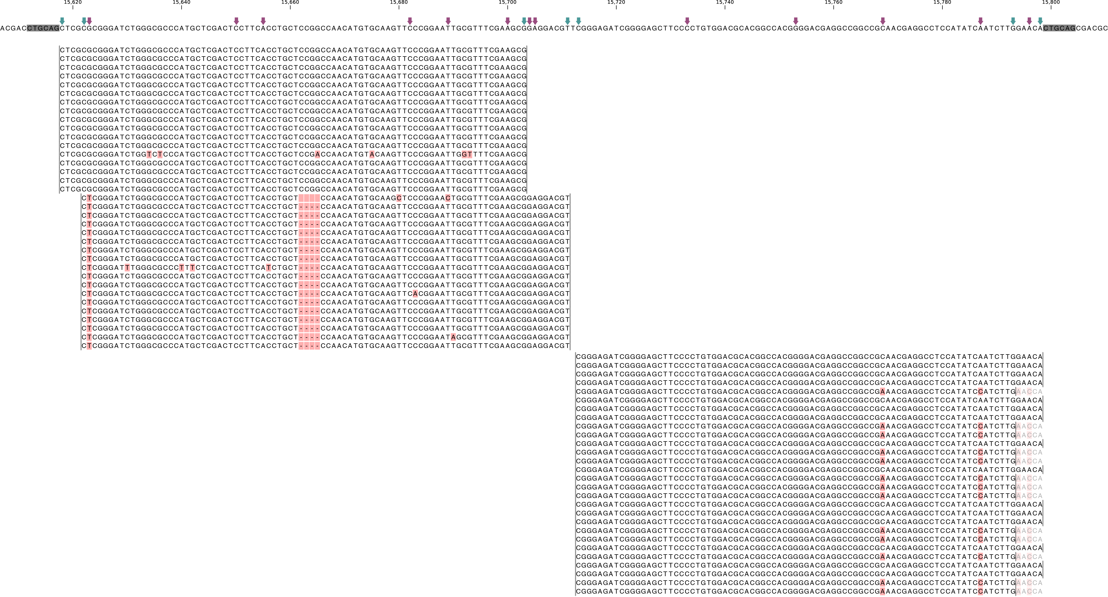 BAM file containing the alignments of single-end GBS read data of an individual genotype, illustrating the presence of various haplotypes. The GBS fragment is flanked on both sides by a Pst I restriction site (grey box) and contains two independent loci. The first locus contains single-end reads mapped on the forward (+) strand.The second locus contains reads mapped on the reverse (-) strand. Haplotypes are defined by combinations of neighboring SMAPs (light blue arrows) and SNPs (purple arrows). A SMAP at position 15622 is created by an InDel close to the 5’ of the GBS-fragment combined with a misalignment (see SMAP delineate for details), while a SMAP at position 15792 is created by consistent soft clipping in a particular haplotype. Various sequencing read errors are present at positions other than the identified SNP positions, but are ignored as they are not listed in the VCF file. One of the SNPs (15793) is located in the soft clipped region.
Commands & options
Mandatory options for SMAP haplotype-sites
-mapping_orientation must always be used to specify if strandedness of read mapping should be considered for haplotyping. -mapping_orientation stranded means that only reads will be considered that map on the same strand as indicated per locus in the SMAP BED file. -mapping_orientation ignore should be used to collect all reads per locus independent of the strand that the reads are mapped on (i.e. ignoring their mapping orientation). See the section on strandedness for more information.-mapping_orientation ignore for PE HiPlex reads that were merged before mapping (by e.g. PEAR).-mapping_orientation ignore for single-end, paired-end reads mapped separately, or reads that were merged before mapping (by e.g. PEAR).-mapping_orientation stranded for single-end or paired-end reads mapped separately.-mapping_orientation ignore for reads that were merged before mapping (by e.g. PEAR).-partial must always be used to specify if reads are expected to be aligned at both outer positions of the locus (HiPlex, Shotgun SNPs in sliding frames) or if reads are expected to display read mapping polymorphisms along the locus (GBS, Shotgun SVs).-partial exclude means that only reads are considered for haplotyping that completely cover the locus including both start and end points. Partially mapped reads are excluded. (see also HiPlex and Shotgun SNPs)-partial include means that all reads are considered for haplotyping, including reads that only partially cover the locus. (see also GBS and Shotgun SVs)-partial exclude for HiPlex because reads amplified with both primers are expected to cover the entire region between the primers. This is scored by being “present” in the read-reference aligned nucleotide pair on the two SMAP positions (just downstream of the forward primer, and just upstream of the reverse primer). Reads with partial alignments are considered amplification, sequencing, or read trimming artefacts, and are excluded from evaluation in the haplotype tables.-partial include for GBS because you must include reads with mapping position polymorphisms in the haplotype table.General options
alignments_dir ############# (str) ### location of the directory containing BAM and BAI files. All BAM files should be in the same directory. Positional mandatory argument, should be the first argument after smap haplotype-sites [no default].bed ##################### (str) ### location of the BED file containing sites for which haplotypes will be reconstructed. For GBS experiments, the BED file should be generated using SMAP delineate. For HiPlex data, a BED6 file can be provided, with the 4th and 5th column being blank and the chromosome name, locus start position site, locus end position site and strand information populating the first, second, third and sixth column respectively. Positional mandatory argument, should be the second argument after smap haplotype-sites.vcf ##################### (str) ### location of the VCF file (in VCFv4.2 format) containing variant positions. It should contain at least the first 9 columns listing the SNP positions, sample-specific genotype calls across the sampleset are not required. Positional mandatory argument, should be the third argument after smap haplotype-sites.-p, --processes ########### (int) ### Number of parallel processes [1].--plot ######################### Select which plots are to be generated. Choosing “nothing” disables plot generation. Passing “summary” only generates graphs with information for all samples while “all” will also enable generate per-sample plots [default “summary”].-t, --plot_type ################## Use this option to choose plot format, choices are png and pdf [png].-o, --out ############### (str) ### Basename of the output file without extension [SMAP_haplotype_sites].-u, --undefined_representation ####### Value to use for non-existing or masked data [NaN].-h, --help ##################### Show the full list of options. Disregards all other parameters.-v, --version ################### Show the version. Disregards all other parameters.--debug ######################## Enable verbose logging.Filtering options
-q, --min_mapping_quality #### (int) ### Minimum .bam mapping quality to retain reads for analysis [30].--no_indels ##################### Use this option if you want to exclude haplotypes that contain an InDel at the given SNP/SMAP positions. These reads are also ignored to evaluate the minimal read count [default off; indels are included in output].-j, --min_distinct_haplotypes # (int) ### Minimal number of distinct haplotypes per locus across all samples. Loci that do not fit this criterium are removed from the final output [0].-k, --max_distinct_haplotypes # (int) ### Maximal number of distinct haplotypes per locus across all samples. Loci that do not fit this criterium are removed from the final output [inf].-c, --min_read_count ####### (int) ### Minimal total number of reads per locus per sample [0].-d, --max_read_count ####### (int) ### Maximal number of reads per locus per sample, read count is calculated after filtering out the low frequency haplotypes (-f) [inf].-f, --min_haplotype_frequency # (float) ## Set minimal HF (in %) to retain the haplotype in the genotyping matrix. Haplotypes above this threshold in at least one of the samples are retained. Haplotypes that never reach this threshold in any of the samples are removed [0].-m, --mask_frequency ####### (float) ## Mask haplotype frequency values below this threshold for individual samples to remove noise from the final output. Haplotype frequency values below this threshold are set to -u. Haplotypes are not removed based on this value, use --min_haplotype_frequency for this purpose instead.Options for discrete calling in individual samples
This option is primarily supported for diploids, triploids and tetraploids. Users can define their own custom frequency interval bounds for species with a higher ploidy, but this requires optimization based on the observed haplotype frequency distributions.
-e, –-discrete_calls ### (str) ### Set to “dominant” to transform haplotype frequency values into presence(1)/absence(0) calls per allele, or “dosage” to indicate the allele copy number.
-i, --frequency_interval_bounds ## Frequency interval bounds for classifying the read frequencies into discrete calls. Custom thresholds can be defined by passing one or more space-separated integers or floats which represent relative frequencies in percentage. For dominant calling, one value should be specified. For dosage calling, an even total number of four or more thresholds should be specified. Defaults are used by passing either “diploid”, “triploid”, or “tetraploid”. The default value for dominant calling (see discrete_calls argument) is 10, regardless if “diploid”, “triploid” or “tetraploid” is used. For dosage calling, the default for diploids is “10 10 90 90”, for triploids “12.5 12.5 50.0 50.0 87.5 87.5”, and for tetraploids “12.5 12.5 37.5 37.5 62.5 62.5 87.5 87.5”.
-z, --dosage_filter #### (int) ### Mask dosage calls in the loci for which the total allele count for a given locus at a given sample differs from the defined value. For example, in diploid organisms the total allele copy number must be 2, in triploid organisms the total dosage call must be 3, and in tetraploids the total allele copy number must be 4 [default no filtering].
--locus_correctness ###### (int) ### Threshold value: % of samples with locus correctness. Create a new .bed file defining only the loci that were correctly dosage called (-z) in at least the defined percentage of samples [default no filtering].
--cervus ################# ### Transform discrete genotype call table to a multi-allelic format that can be used as input for Cervus. Haplotypes are transformed to letters of the alphabet (a-z).
--frequency_interval_bounds in practical examples and additional information on the dosage filter can be found in the section on recommendations.
Example commands
HiPlex
smap haplotype-sites /directory/with/BAMs/ /location/of/BED /location/of/VCF -mapping_orientation ignore -partial exclude --no_indels --min_read_count 30 -f 5 -p 8 --min_distinct_haplotypes 2 --plot_type png --plot all -o 2n_pool_HiPlex_NI_NP
smap haplotype-sites /directory/with/BAMs/ /location/of/BED /location/of/VCF -mapping_orientation ignore -partial exclude --min_read_count 10 -f 5 -p 8 --min_distinct_haplotypes 2 --plot_type png --plot all -o 2n_ind_HiPlex_NI_NP_DOMdiplo --discrete_calls dominant --frequency_interval_bounds 10
smap haplotype-sites /directory/with/BAMs/ /location/of/BED /location/of/VCF -mapping_orientation ignore -partial exclude --no_indels --min_read_count 10 -f 5 -p 8 --min_distinct_haplotypes 2 --plot_type png --plot all -o 2n_ind_HiPlex_NI_NP_DOSdiplo --discrete_calls dosage --frequency_interval_bounds 10 10 90 90 --dosage_filter 2
smap haplotype-sites /directory/with/BAMs/ /location/of/BED /location/of/VCF -mapping_orientation ignore -partial exclude --no_indels --min_read_count 15 -f 5 -p 8 --min_distinct_haplotypes 2 --plot_type png --plot all -o 2n_ind_HiPlex_NI_NP_DOMtriplo --discrete_calls dominant --frequency_interval_bounds 10
smap haplotype-sites /directory/with/BAMs/ /location/of/BED /location/of/VCF -mapping_orientation ignore -partial exclude --no_indels --min_read_count 15 -f 5 -p 8 --min_distinct_haplotypes 2 --plot_type png --plot all -o 2n_ind_HiPlex_NI_NP_DOStriplo --discrete_calls dosage --frequency_interval_bounds 12.5 12.5 50.0 50.0 87.5 87.5 --dosage_filter 3
smap haplotype-sites /directory/with/BAMs/ /location/of/BED /location/of/VCF -mapping_orientation ignore -partial exclude --no_indels --discrete_calls dominant --frequency_interval_bounds 10 --min_read_count 20 -f 5 -p 8 --min_distinct_haplotypes 2 --plot_type png --plot all -o 4n_ind__NI_NP_DOMtetra
smap haplotype-sites /directory/with/BAMs/ /location/of/BED /location/of/VCF -mapping_orientation ignore -partial exclude --no_indels --discrete_calls dosage --frequency_interval_bounds 12.5 12.5 37.5 37.5 62.5 62.5 87.5 87.5 --dosage_filter 4 --min_read_count 20 -f 5 -p 8 --min_distinct_haplotypes 2 --plot_type png --plot all -o 4n_ind__NI_NP_DOStetra
Shotgun
smap haplotype-sites /directory/with/BAMs/ /location/of/BED /location/of/VCF -mapping_orientation stranded -partial include --min_read_count 10 -f 5 -p 8 --min_distinct_haplotypes 2 --plot_type png --plot all -o 2n_ind_WGS_SE_NI_DOMdiplo --discrete_calls dominant --frequency_interval_bounds 10
smap haplotype-sites /directory/with/BAMs/ /location/of/BED /location/of/VCF -mapping_orientation stranded -partial include --min_read_count 10 -f 5 -p 8 --min_distinct_haplotypes 2 --plot_type png --plot all -o 2n_ind_WGS_SE_NI_DOSdiplo --discrete_calls dosage --frequency_interval_bounds diploid
GBS
smap haplotype-sites /directory/with/BAMs/ /location/of/BED /location/of/VCF -mapping_orientation stranded -partial include --no_indels --min_read_count 30 -f 2 -p 8 --min_distinct_haplotypes 2 --plot_type png --plot all -o 2n_pool_GBS_SE_NI
smap haplotype-sites /directory/with/BAMs/ /location/of/BED /location/of/VCF -mapping_orientation ignore -partial include --no_indels --min_read_count 30 -f 2 -p 8 --min_distinct_haplotypes 2 --plot_type png --plot all -o 2n_pools_GBS_PE_NI
smap haplotype-sites /directory/with/BAMs/ /location/of/BED /location/of/VCF -mapping_orientation ignore -partial include --no_indels --min_read_count 30 -f 2 -p 8 --min_distinct_haplotypes 2 --plot_type png --plot all -o 4n_pools_GBS_PE_NI
smap haplotype-sites /directory/with/BAMs/ /location/of/BED /location/of/VCF -mapping_orientation stranded -partial include --no_indels --min_read_count 10 -f 5 -p 8 --min_distinct_haplotypes 2 --plot_type png --plot all -o 2n_ind_GBS_SE_NI_DOSdiplo --discrete_calls dosage --frequency_interval_bounds 10 10 90 90 --dosage_filter 2
smap haplotype-sites /directory/with/BAMs/ /location/of/BED /location/of/VCF -mapping_orientation ignore -partial include --no_indels --min_read_count 10 -f 5 -p 8 --min_distinct_haplotypes 2 --plot_type png --plot all -o 2n_ind_GBS_PE_NI_DOMdiplo --discrete_calls dominant --frequency_interval_bounds 10
smap haplotype-sites /directory/with/BAMs/ /location/of/BED /location/of/VCF -mapping_orientation ignore -partial include --no_indels --min_read_count 10 -f 5 -p 8 --min_distinct_haplotypes 2 --plot_type png --plot all -o 2n_ind_GBS_PE_NI_DOSdiplo --discrete_calls dosage --frequency_interval_bounds 10 10 90 90 --dosage_filter 2
smap haplotype-sites /directory/with/BAMs/ /location/of/BED /location/of/VCF -mapping_orientation ignore -partial include --no_indels --discrete_calls dominant --frequency_interval_bounds 10 --min_read_count 10 -f 5 -p 8 --min_distinct_haplotypes 2 --plot_type png --plot all -o 4n_ind_GBS_PE_NI_DOMtetra
smap haplotype-sites /directory/with/BAMs/ /location/of/BED /location/of/VCF -mapping_orientation ignore -partial include --no_indels --discrete_calls dosage --frequency_interval_bounds 12.5 12.5 37.5 37.5 62.5 62.5 87.5 87.5 --dosage_filter 4 --min_read_count 10 -f 5 -p 8 --min_distinct_haplotypes 2 --plot_type png --plot all -o 4n_ind_GBS_PE_NI_DOStetra
Summary of Commands
A typical command line example :
smap haplotype-sites /directory/with/BAMs/ /location/of/BED /location/of/VCF -mapping_orientation stranded --no_indels -c 10 -f 5 -p 8 --plot_type png -partial include --min_distinct_haplotypes 2 -o haplotypes_SampleSet1
Output
Tabular output
By default, SMAP haplotype-sites will return two .tsv files.
haplotype counts
Read_counts_cx_fx_mx.tsv (with x the value per option used in the analysis) contains the read counts (-c) and haplotype frequency (-f) filtered and/or masked (-m) read counts per haplotype per locus as defined in the BED file from SMAP delineate.
This is the file structure:
Locus
Haplotypes
Sample1
Sample2
Sample..
Chr1:100-200_+
00010
0
13
34
Chr1:100-200_+
01000
19
90
28
Chr1:100-200_+
00110
60
0
23
Chr1:450-600_+
0010
70
63
87
Chr1:450-600_+
0110
108
22
134
relative haplotype frequency
Haplotype_frequencies_cx_fx_mx.tsv contains the relative frequency per haplotype per locus in sample (based on the corresponding count table: Read_counts_cx_fx_mx.tsv). The transformation to relative frequency per locus-sample combination inherently normalizes for differences in total number of mapped reads across samples, and differences in amplification efficiency across loci. This is the file structure:
Locus
Haplotypes
Sample1
Sample2
Sample..
Chr1:100-200_+
00010
0
0.13
0.40
Chr1:100-200_+
01000
0.24
0.87
0.33
Chr1:100-200_+
00110
0.76
0
0.27
Chr1:450-600_+
0010
0.39
0.74
0.39
Chr1:450-600_+
0110
0.61
0.26
0.61
For individuals, if the option --discrete_calls is used, the program will return three additional .tsv files. Their content and order of creation is shown in this scheme.
haplotype total discrete callsThe first file is called haplotypes_cx_fx_mx_discrete_calls._total.tsv and this file contains the total dosage calls, obtained after transforming haplotype frequencies into discrete calls, using the defined--frequency_interval_bounds. The total sum of discrete dosage calls is expected to be 2 in diploids and 4 in tetraploids.
Locus
Sample1
Sample2
Sample..
Chr1:100-200_+
2
2
3
Chr1:450-600_+
2
2
2
haplotype discrete callsThe second file is haplotypes_cx_fx_mx-discrete_calls_filtered.tsv, which lists the discrete calls per locus per sample after--dosage_filterhas removed loci per sample with an unexpected number of haplotype calls (as listed in haplotypes_cx_fx_mx_discrete_calls_total.tsv). The expected number of calls is set with option-z[use 2 for diploids, 3 for triploids, 4 for tetraploids].
Locus
Haplotypes
Sample1
Sample2
Sample..
Chr1:100-200_+
00010
0
1
NA
Chr1:100-200_+
01000
1
1
NA
Chr1:100-200_+
00110
1
0
NA
Chr1:450-600_+
0010
1
1
1
Chr1:450-600_+
0110
1
1
1
population haplotype frequenciesThe third file, haplotypes_cx_fx_mx_Pop_HF.tsv, lists the population haplotype frequencies (over all individual samples) based on the total number of discrete haplotype calls relative to the total number of calls per locus.
Locus
Haplotypes
Pop_HF
count
Chr1:100-200_+
00010
25.0
4
Chr1:100-200_+
01000
50.0
4
Chr1:100-200_+
00110
25.0
4
Chr1:450-600_+
0010
50.0
6
Chr1:450-600_+
0110
50.0
6
For individuals, if the option--locus_correctnessis used in combination with--discrete_callsand--frequency_interval_bounds, the programm will create a new .bed file haplotypes_cx_fx_mx_correctnessx_loci.bed (loci filtered from the input .bed file) containing only the loci that were correctly dosage called (-z) in at least the defined percentage of samples. See above.Loci with correct calls across the sample set
Reference
Start
End
HiPlex_locus_name
Mean_read_depth
Strand
SMAPs
Completeness
nr_SMAPs
Name
Chr1
99
200
Chr1:100-200_+
.
+
100,200
.
2
HiPlex_Set1
Chr1
449
600
Chr1:450-600_+
.
+
450,600
.
2
HiPlex_Set1
Graphical output
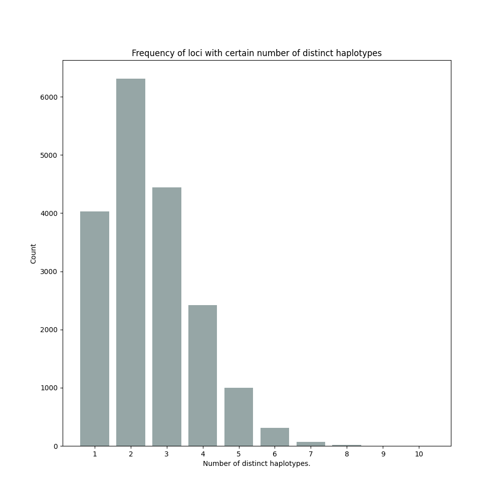
haplotype diversity
By default, SMAP haplotype-sites will generate graphical output summarizing haplotype diversity. haplotype_counts_discrete_calls_filtered.barplot.png shows a histogram of the number of distinct haplotypes per locus across all samples.
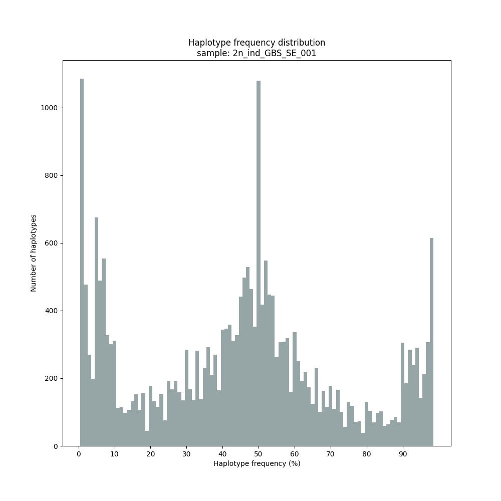
haplotype frequency distribution per sample
Graphical output of the haplotype frequency distribution for each individual sample can be switched on using the option --plot_all. sample_haplotype_frequency_distribution.png shows the haplotype frequency distribution across all loci detected per sample. It is the graphical representation of each sample-specific column in haplotypes_cx_fx_mx.tsv. Using the option --discrete_calls, this plot will also show the defined discrete calling boundaries.
quality of genotype calls per locus and per sample (only for individuals)
After discrete genotype calling with option --discrete_calls, SMAP haplotype-sites will evaluate the observed sum of discrete dosage calls per locus per sample versus the expected value per locus (set with option -z, recommended use: 2 for diploid, 4 for tetraploid).
The quality of genotype calls per sample is calculated in two ways: the fraction of loci with calls in that sample versus the total number of loci across all samples (sample_call_completeness); the fraction of loci with expected sum of discrete dosage calls (-z) versus the total number of observed loci in that sample (sample_call_correctness.tsv). These scores are calculated separately per sample, and SMAP haplotype-sites plots the distribution of those scores across the sample set (sample_call_completeness.png; sample_call_correctness.png).
Similarly, the quality of genotype calls per locus is calculated in two ways: the fraction of samples with calls for that locus versus the total number of samples (locus_call_completeness); the fraction of samples with expected sum of discrete dosage calls (-z) versus the total number of observed samples for that locus (locus_call_correctness.tsv). These scores are calculated separately per locus, and SMAP haplotype-sites plots the distribution of those scores across the locus set (locus_call_completeness.png; locus_call_correctness.png).
Both graphs and the corresponding tables (one for samples and one for loci) can be evaluated to identify poorly performing samples and/or loci. We recommend to eliminate these from further analysis by removing BAM files from the run directory and/or loci from the SMAP delineate BED file with SMAPs, and iterate through rounds of data analysis combined with sample and locus quality control.
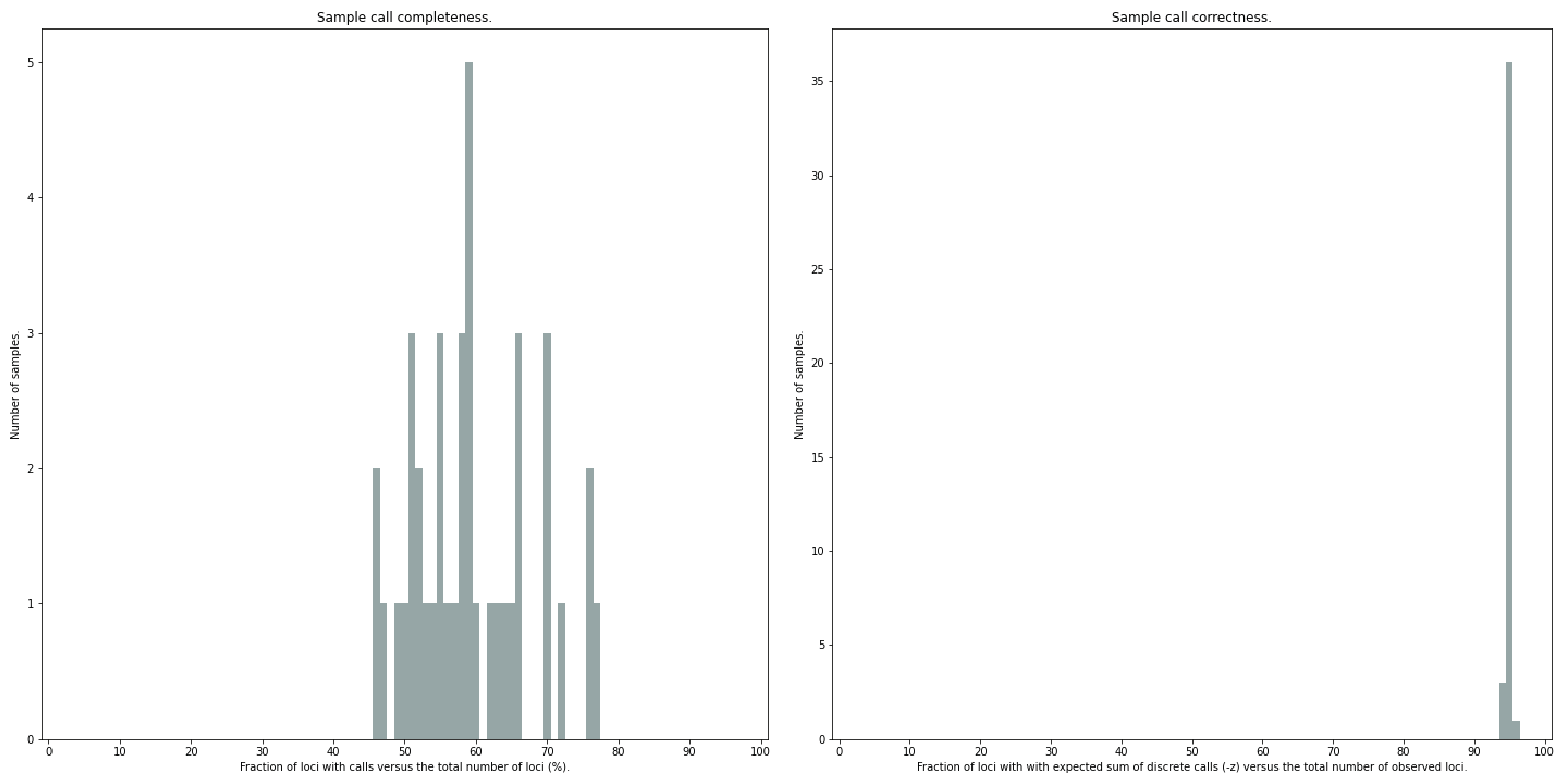
The sample call completeness plot shows the percentage of loci that have data across the samples after all filters. In read depth-saturated, low diversity datasets, the majority of samples should have high locus completeness and there should not be much variation in completeness between samples. In a high diversity or read depth-unsaturated sample set, locus completeness per sample will be lower and more spread out.
The sample call correctness plot displays the percentage of correctly dosage called (-z) loci across the sampleset. Loci are only masked in samples with a dosage value different from -z but remain in the data set for all other samples with the expected dosage value.
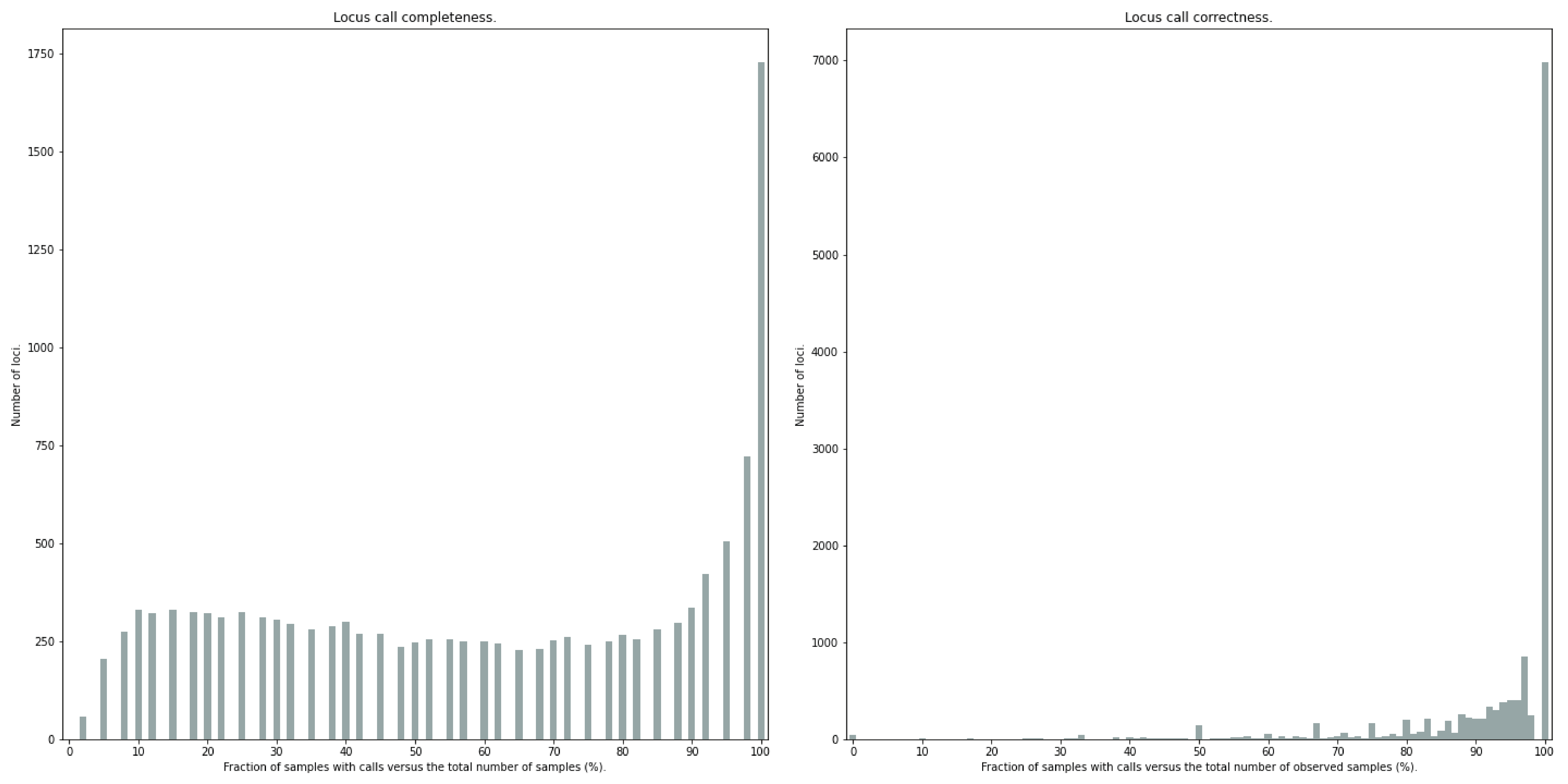
The locus call completeness plot displays the percentage of samples that have data (after every filter) on a locus for every locus. In read depth-saturated, low diversity sample sets, the majority of samples should have many high completeness loci and few low completeness loci. In a high diversity or read depth-unsaturated sample set, many loci will have a low completeness.
The locus call correctness plot shows the percentage of samples that were correctly dosage called (-z) across the locus set. Loci with low correctness values indicate potential genotype calling artefacts and should be removed from the data set.