Scope & Usage
Scope
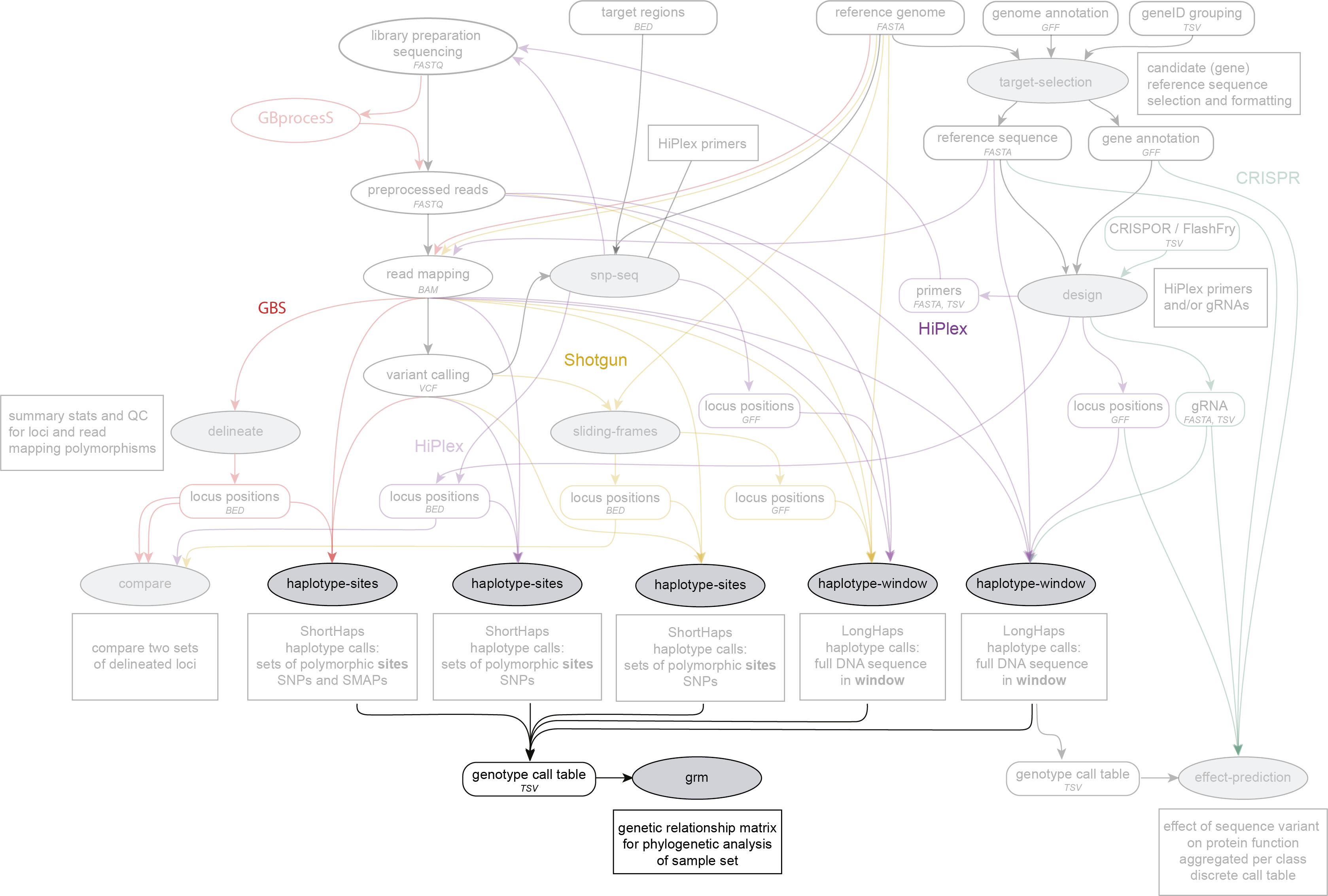
Integration in the SMAP workflow
Example input files
Reference |
Locus |
Haplotypes |
ind1 |
ind2 |
ind3 |
ind4 |
ind5 |
ind6 |
ind7 |
ind8 |
ind9 |
ind10 |
ind11 |
ind12 |
ind13 |
ind14 |
ind15 |
ind16 |
ind17 |
ind18 |
ind19 |
|---|---|---|---|---|---|---|---|---|---|---|---|---|---|---|---|---|---|---|---|---|---|
chrom1 |
locus1 |
1000 |
2 |
0 |
0 |
1 |
2 |
2 |
2 |
1 |
1 |
2 |
0 |
0 |
0 |
0 |
0 |
0 |
0 |
2 |
|
chrom1 |
locus1 |
1001 |
0 |
0 |
2 |
0 |
0 |
0 |
0 |
1 |
1 |
0 |
2 |
0 |
0 |
2 |
1 |
0 |
2 |
0 |
|
chrom1 |
locus1 |
1011 |
0 |
2 |
0 |
0 |
0 |
0 |
0 |
0 |
0 |
0 |
0 |
1 |
0 |
0 |
1 |
2 |
0 |
0 |
|
chrom1 |
locus1 |
1111 |
0 |
0 |
0 |
1 |
0 |
0 |
0 |
0 |
0 |
0 |
0 |
1 |
2 |
0 |
0 |
0 |
0 |
0 |
|
chrom1 |
locus2 |
1000 |
2 |
2 |
0 |
0 |
0 |
0 |
0 |
0 |
0 |
0 |
0 |
0 |
0 |
0 |
0 |
0 |
0 |
0 |
0 |
chrom1 |
locus2 |
1001 |
0 |
0 |
2 |
2 |
1 |
0 |
0 |
0 |
0 |
0 |
0 |
1 |
0 |
2 |
0 |
0 |
2 |
1 |
0 |
chrom1 |
locus2 |
1011 |
0 |
0 |
0 |
0 |
1 |
2 |
2 |
2 |
1 |
0 |
2 |
1 |
2 |
0 |
2 |
2 |
0 |
1 |
2 |
chrom1 |
locus2 |
1111 |
0 |
0 |
0 |
0 |
0 |
0 |
0 |
0 |
1 |
1 |
0 |
0 |
0 |
0 |
0 |
0 |
0 |
0 |
0 |
chrom1 |
locus2 |
1101 |
0 |
0 |
0 |
0 |
0 |
0 |
0 |
0 |
0 |
1 |
0 |
0 |
0 |
0 |
0 |
0 |
0 |
0 |
0 |
chrom1 |
locus3 |
1000 |
2 |
2 |
2 |
2 |
0 |
0 |
1 |
1 |
1 |
2 |
0 |
0 |
2 |
0 |
0 |
0 |
2 |
0 |
2 |
chrom1 |
locus3 |
1001 |
0 |
0 |
0 |
0 |
2 |
2 |
0 |
0 |
0 |
0 |
2 |
2 |
0 |
2 |
2 |
0 |
0 |
2 |
0 |
chrom1 |
locus3 |
1011 |
0 |
0 |
0 |
0 |
0 |
0 |
1 |
1 |
1 |
0 |
0 |
0 |
0 |
0 |
0 |
2 |
0 |
0 |
0 |
chrom1 |
locus4 |
1000 |
0 |
0 |
2 |
2 |
2 |
2 |
2 |
2 |
2 |
2 |
2 |
0 |
2 |
2 |
2 |
2 |
2 |
2 |
1 |
chrom1 |
locus4 |
1001 |
2 |
2 |
0 |
0 |
0 |
0 |
0 |
0 |
0 |
0 |
0 |
2 |
0 |
0 |
0 |
0 |
0 |
0 |
1 |
chrom1 |
locus5 |
1000 |
2 |
0 |
0 |
2 |
2 |
2 |
0 |
1 |
2 |
2 |
0 |
0 |
0 |
1 |
0 |
0 |
0 |
0 |
0 |
chrom1 |
locus5 |
1001 |
0 |
2 |
1 |
0 |
0 |
0 |
0 |
0 |
0 |
0 |
0 |
0 |
0 |
0 |
2 |
0 |
2 |
2 |
2 |
chrom1 |
locus5 |
1011 |
0 |
0 |
1 |
0 |
0 |
0 |
0 |
0 |
0 |
0 |
0 |
0 |
0 |
1 |
0 |
2 |
0 |
0 |
0 |
chrom1 |
locus5 |
1111 |
0 |
0 |
0 |
0 |
0 |
0 |
2 |
0 |
0 |
0 |
0 |
2 |
2 |
0 |
0 |
0 |
0 |
0 |
0 |
chrom1 |
locus5 |
1101 |
0 |
0 |
0 |
0 |
0 |
0 |
0 |
1 |
0 |
0 |
2 |
0 |
0 |
0 |
0 |
0 |
0 |
0 |
0 |
chrom1 |
locus6 |
1000 |
2 |
2 |
2 |
2 |
2 |
0 |
0 |
0 |
2 |
2 |
0 |
0 |
2 |
1 |
2 |
0 |
0 |
0 |
|
chrom1 |
locus6 |
1001 |
0 |
0 |
0 |
0 |
0 |
1 |
1 |
1 |
0 |
0 |
2 |
0 |
0 |
1 |
0 |
2 |
0 |
0 |
|
chrom1 |
locus6 |
1011 |
0 |
0 |
0 |
0 |
0 |
1 |
1 |
1 |
0 |
0 |
0 |
2 |
0 |
0 |
0 |
0 |
2 |
2 |
|
chrom1 |
locus7 |
1000 |
2 |
2 |
0 |
0 |
2 |
2 |
2 |
2 |
2 |
2 |
2 |
2 |
2 |
2 |
2 |
2 |
2 |
2 |
2 |
chrom1 |
locus7 |
1001 |
0 |
0 |
2 |
2 |
0 |
0 |
0 |
0 |
0 |
0 |
0 |
0 |
0 |
0 |
0 |
0 |
0 |
0 |
0 |
chrom1 |
locus8 |
1000 |
0 |
0 |
0 |
0 |
1 |
0 |
0 |
0 |
0 |
0 |
2 |
0 |
0 |
0 |
0 |
0 |
0 |
0 |
2 |
chrom1 |
locus8 |
1001 |
0 |
0 |
0 |
0 |
1 |
2 |
0 |
0 |
0 |
0 |
0 |
2 |
2 |
0 |
1 |
0 |
2 |
0 |
0 |
chrom1 |
locus8 |
1011 |
2 |
2 |
2 |
2 |
0 |
0 |
0 |
0 |
0 |
0 |
0 |
0 |
0 |
2 |
0 |
0 |
0 |
2 |
0 |
chrom1 |
locus8 |
1111 |
0 |
0 |
0 |
0 |
0 |
0 |
2 |
2 |
2 |
0 |
0 |
0 |
0 |
0 |
1 |
0 |
0 |
0 |
0 |
chrom1 |
locus8 |
1101 |
0 |
0 |
0 |
0 |
0 |
0 |
0 |
0 |
0 |
2 |
0 |
0 |
0 |
0 |
0 |
2 |
0 |
0 |
0 |
chrom1 |
locus9 |
1000 |
2 |
0 |
2 |
0 |
0 |
0 |
2 |
2 |
2 |
2 |
2 |
2 |
2 |
2 |
2 |
2 |
2 |
2 |
2 |
chrom1 |
locus9 |
1001 |
0 |
0 |
0 |
1 |
0 |
0 |
0 |
0 |
0 |
0 |
0 |
0 |
0 |
0 |
0 |
0 |
0 |
0 |
0 |
chrom1 |
locus9 |
1011 |
0 |
0 |
0 |
1 |
0 |
0 |
0 |
0 |
0 |
0 |
0 |
0 |
0 |
0 |
0 |
0 |
0 |
0 |
0 |
chrom1 |
locus9 |
1111 |
0 |
0 |
0 |
0 |
2 |
2 |
0 |
0 |
0 |
0 |
0 |
0 |
0 |
0 |
0 |
0 |
0 |
0 |
0 |
chrom1 |
locus9 |
1101 |
0 |
2 |
0 |
0 |
0 |
0 |
0 |
0 |
0 |
0 |
0 |
0 |
0 |
0 |
0 |
0 |
0 |
0 |
0 |
chrom1 |
locus10 |
1000 |
2 |
2 |
0 |
0 |
1 |
0 |
0 |
1 |
0 |
2 |
0 |
0 |
2 |
0 |
2 |
0 |
2 |
1 |
2 |
chrom1 |
locus10 |
1001 |
0 |
0 |
2 |
2 |
0 |
0 |
0 |
0 |
0 |
0 |
2 |
2 |
0 |
2 |
0 |
0 |
0 |
1 |
0 |
chrom1 |
locus10 |
1011 |
0 |
0 |
0 |
0 |
1 |
2 |
2 |
1 |
2 |
0 |
0 |
0 |
0 |
0 |
0 |
2 |
0 |
0 |
0 |
chrom1 |
locus11 |
1000 |
2 |
2 |
2 |
2 |
2 |
2 |
1 |
2 |
2 |
2 |
0 |
0 |
0 |
0 |
0 |
0 |
0 |
0 |
|
chrom1 |
locus11 |
1001 |
0 |
0 |
0 |
0 |
0 |
0 |
1 |
0 |
0 |
0 |
0 |
0 |
0 |
0 |
0 |
0 |
0 |
0 |
|
chrom1 |
locus11 |
1011 |
0 |
0 |
0 |
0 |
0 |
0 |
0 |
0 |
0 |
0 |
2 |
2 |
2 |
1 |
2 |
1 |
0 |
2 |
|
chrom1 |
locus11 |
1111 |
0 |
0 |
0 |
0 |
0 |
0 |
0 |
0 |
0 |
0 |
0 |
0 |
0 |
1 |
0 |
1 |
2 |
0 |
|
chrom1 |
locus12 |
1000 |
0 |
0 |
0 |
0 |
0 |
0 |
0 |
0 |
1 |
0 |
0 |
0 |
1 |
0 |
0 |
0 |
0 |
0 |
0 |
chrom1 |
locus12 |
1001 |
0 |
0 |
0 |
0 |
0 |
0 |
0 |
0 |
1 |
0 |
0 |
2 |
0 |
0 |
0 |
1 |
0 |
0 |
0 |
chrom1 |
locus12 |
1011 |
2 |
1 |
0 |
2 |
0 |
0 |
2 |
2 |
0 |
2 |
2 |
0 |
1 |
2 |
2 |
1 |
2 |
2 |
2 |
chrom1 |
locus12 |
1111 |
0 |
0 |
2 |
0 |
2 |
2 |
0 |
0 |
0 |
0 |
0 |
0 |
0 |
0 |
0 |
0 |
0 |
0 |
0 |
chrom1 |
locus12 |
1101 |
0 |
1 |
0 |
0 |
0 |
0 |
0 |
0 |
0 |
0 |
0 |
0 |
0 |
0 |
0 |
0 |
0 |
0 |
0 |
Options may be given in any order.
--samples to select a subset of samples, to change the sample order or names, or combine data of multiple samples into a single sample (e.g. joining replicates into a single representative sample).
ind1
ind2
ind3
ind6
ind7
ind9
ind10
ind5
cultivar001_plant1
ind6
cultivar001_plant2
ind7
cultivarX
ind8
cultivarY
ind9
cultivarZ
ind1
wild01
ind2
wild02
ind3
wild03_rep1
ind4
wild03_rep2
ind10
varietyB
ind1
groupI
ind2
groupI
ind3
groupII
ind4
groupII
ind5
groupIII
ind6
groupIII
ind7
groupIV
ind8
groupIV
ind9
groupIV
ind10
groupV
--loci to only analyze a subset of loci.
Locus1
Locus2
Locus5
Locus6
Locus7
Locus10
Commands & options
Mandatory options for SMAP grm
-t, --table ########### (str) ### Name of the haplotype call table obtained with SMAP haplotype-sites or SMAP haplotype-window in the input directory [no default].
Basic command to run SMAP grm with default parameters:
smap grm --table /PATH/TO/Haplotype_table.tsv
Command line options
See tabs below for detailed command line options.
-i,--input_directory#### (str) ### Path to the directory containing the haplotype call table, the--samplestext file, and/or the--locitext file [current directory].-n,--samples########## (str) ### Name of a tab-delimited text file in the input directory defining the order of the (new) sample IDs in the matrix: first column = old IDs, second column (optional) = new IDs [no list provided, the order of sample IDs in the grm equals their order in the haplotype call table].-l,--loci############ (str) ### Name of a tab-delimited text file in the input directory containing a one-column list of locus IDs formatted as in the haplotype call table [no list provided].-p,--processes######### (int) ### Number of parallel processes [4].-t,--plot_type############### Use this option to choose plot format, choices are png and pdf [png].-h,--help################### Show the full list of options. Disregards all other parameters.-v,--version################# Show the version. Disregards all other parameters.
Options may be given in any order.
-lc,--locus_completeness#### (float) ###.. Minimum proportion of samples with haplotype data in a locus. Loci with less data are removed [all loci are included].-sc,--sample_completeness##### (int) ###.. Minimum number of loci with haplotype data in a sample. Samples with less data are removed [all samples are included].--include_non_shared_loci############## Loci with data in only one out of two samples in each comparison are included in genetic similarity and locus information calculations [only loci with data in both samples of each comparison are included in calculations].-s,--similarity_coefficient#### (str) ###. Coefficient used to express pairwise genetic similarity between samples [Jaccard, other options are: Sorensen-Dice and Ochiai].--distance########################.. Convert genetic similarity estimates into genetic distances [no conversion to distances].--distance_method############# (str) ###. Method used for genetic distance calculations [Inversed, other option is: Euclidean].-lic,--locus_information_criterion####### Create a matrix showing the number of loci with shared or unique haplotypes in each comparison Shared: matrix showing the number of loci with shared haplotypes. Unique: matrix showing the number of loci with unique haplotypes [Shared].--partial########################## Include loci in the locus information matrix with at least one shared/unique haplotype [only loci with only shared/unique haplotypes are included].--proportion_informative_loci############ Express the informative locus count as a proportion [locus information content is expressed in absolute numbers].-b,--bootstrap############### (int) ### The number of bootstrap replicates of the genetic similarity/distance matrix [no bootstrap replicates].
Options may be given in any order.
-o,--output_directory#### (str) ### Output directory [current directory].-s,--suffix#### (str) ### Suffix added to all output file names [no suffix added].--print_sample_information#### (str) ### Print the similarity/distance matrix and the number of (shared) loci to the output directory as matrices (Matrix option, .csv file) and/or as plots (Plot option, file type specified by –plot_format option) {Matrix, Plot, All} [Matrix].--print_locus_information#### (str) ### Print locus information to the output directory as a matrix (Matrix option, .csv file) and/or as a plot (Plot option, file type specified by –plot_format option) showing the number of loci with shared or unique haplotypes in each comparison. The locus information per locus can also be printed as a tab-delimited list (List option, .txt file) showing the number of comparisons wherein the locus was informative and the sample IDs with unique haplotypes in all comparisons for each locus {None, Matrix, Plot, List, All} [locus information is not printed].--matrix_format#### (str) ### Format of the similarity/distance matrix {Phylip, Nexus} [Phylip].--plot_format#### (str) ### File format of plots {pdf, png, svg, jpg, jpeg, tif, tiff} [pdf].--mask#### (str) ### Mask values on the main diagonal of each matrix and above (Upper) or below (Lower) the main diagonal {None, Upper, Lower} [no masking].--annotate_matrix_plots############### Annotate the matrix plots with values [no annotations].--no_matrix_plot_labels############### Do not plot labels on the axes of matrix plots [labels are plotted on the axes of matrix plots].--plot_line_curves################# Plot line curves showing the genetic correspondence between two samples in function of a cumulative number of loci [curves are not plotted].--list_line_curves################## Tab-delimited text file containing a list of sample comparisons. first column ID of the first sample, second column ID of the second sample. of which line curves need to be plotted [no list specified, all comparisons are plotted if the--plot_line_curvesoption is specified].--locus_interval###### (int) ### Interval in the number of loci between two consecutive points in the line curves [10].-f,--font###### (str) ### Font used in all plots {Times New Roman, Arial, Calibri, Consolas, Verdana, Helvetica, Comic Sans MS} [Times_New_Roman].--title_fontsize#### (float) ### Title font size in points [12].--label_fontsize#### (float) ### Label font size in points [12].--tick_fontsize#### (float) ### Tick font size in points [8].--legend_fontsize#### (float) ### Legend font size in points [10].--legend_position#### (float,float) ### Pair of coordinates defining the x (first number) and y (second number) position of the legend in the line curve plots [1,1, i.e. position the legend in the top right corner of the plot].-r,--plot_resolution#### (float) ### Plot resolution in dots per inch (dpi) [300].--colour_map#### (str) ### Colour palette used in the matrix plots. The (Perceptually Uniform) Sequential colormaps that are shown on the site of MatPlotLib are accepted [bone].{viridis, plasma, inferno, magma, cividis, Greys, Purples, Blues, Greens, Oranges, Reds, YlOrBr, YlOrRd, OrRd, PuRd, RdPu, BuPu, GnBu, PuBu, YlGnBu, PuBuGn, BuGn, YlGn, binary, gist_yarg, gist_gray, gray, bone, pink, spring, summer, autumn, winter, cool, Wistia, hot, afmhot, gist_heat, copper, PiYG, PRGn, BrBG, PuOr, RdGy, RdBu, RdYlBu, RdYlGn, Spectral, coolwarm, bwr, seismic, twilight, twilight_shifted, hsv}
Options may be given in any order.
Example commands
Usage:
smap grm -t, --table TABLE [-i INPUT_DIRECTORY] [-n SAMPLES] [-l LOCI] [-lc LOCUS_COMPLETENESS] [-sc SAMPLE_COMPLETENESS] [--include_non_shared_loci] [--similarity_coefficient {Jaccard, Sorensen-Dice, Ochiai}] [--distance] [--distance_method {Inversed, Euclidean}] [-lic LOCUS_INFORMATION_CRITERION {Shared, Unique}] [--partial] [--proportion_informative_loci] [-b BOOTSTRAP] [-p PROCESSES] [-o OUTPUT_DIRECTORY] [-s SUFFIX] [--print_sample_information {Matrix, Plot, All}] [--print_locus_information {None, Matrix, Plot, List, All}] [--matrix_format {Phylip, Nexus}] [--plot_format {pdf, png, svg, jpg, jpeg, tif, tiff}] [--mask {None, Upper, Lower}] [--annotate_matrix_plots] [--no_matrix_plot_labels] [--plot_line_curves] [--list_line_curves LIST_LINE_CURVES] [--locus_interval LOCUS_INTERVAL] [-f {Times New Roman, Arial, Calibri, Consolas, Verdana, Helvetica, Comic Sans MS}] [--title_fontsize TITLE_FONTSIZE] [--label_fontsize LABEL_FONTSIZE] [--tick_fontsize TICK_FONTSIZE] [--legend_fontsize LEGEND_FONTSIZE] [--legend_position X, Y] [-r PLOT_RESOLUTION] [--colour_map {viridis, plasma, inferno, magma, cividis, Greys, Purples, Blues, Greens, Oranges, Reds, YlOrBr, YlOrRd, OrRd, PuRd, RdPu, BuPu, GnBu, PuBu, YlGnBu, PuBuGn, BuGn, YlGn, binary, gist_yarg, gist_gray, gray, bone, pink, spring, summer, autumn, winter, cool, Wistia, hot, afmhot, gist_heat, copper, PiYG, PRGn, BrBG, PuOr, RdGy, RdBu, RdYlBu, RdYlGn, Spectral, coolwarm, bwr, seismic, twilight, twilight_shifted, hsv}]
Output
All output files are saved to the user-defined output directory (default = current directory).
The output directory is created by the script if the directory did not exist.
The option --print_sample_information creates tab-delimited text files (Matrix, default), or plots heatmaps (Plot), or both (All).
--locus_information_criterion Unique (which creates a matrix showing the number of loci with unique haplotypes in each comparison e.g. locus5 in ind7 uniquely has haplotype d) and only loci with unique haplotypes are counted (complete, default)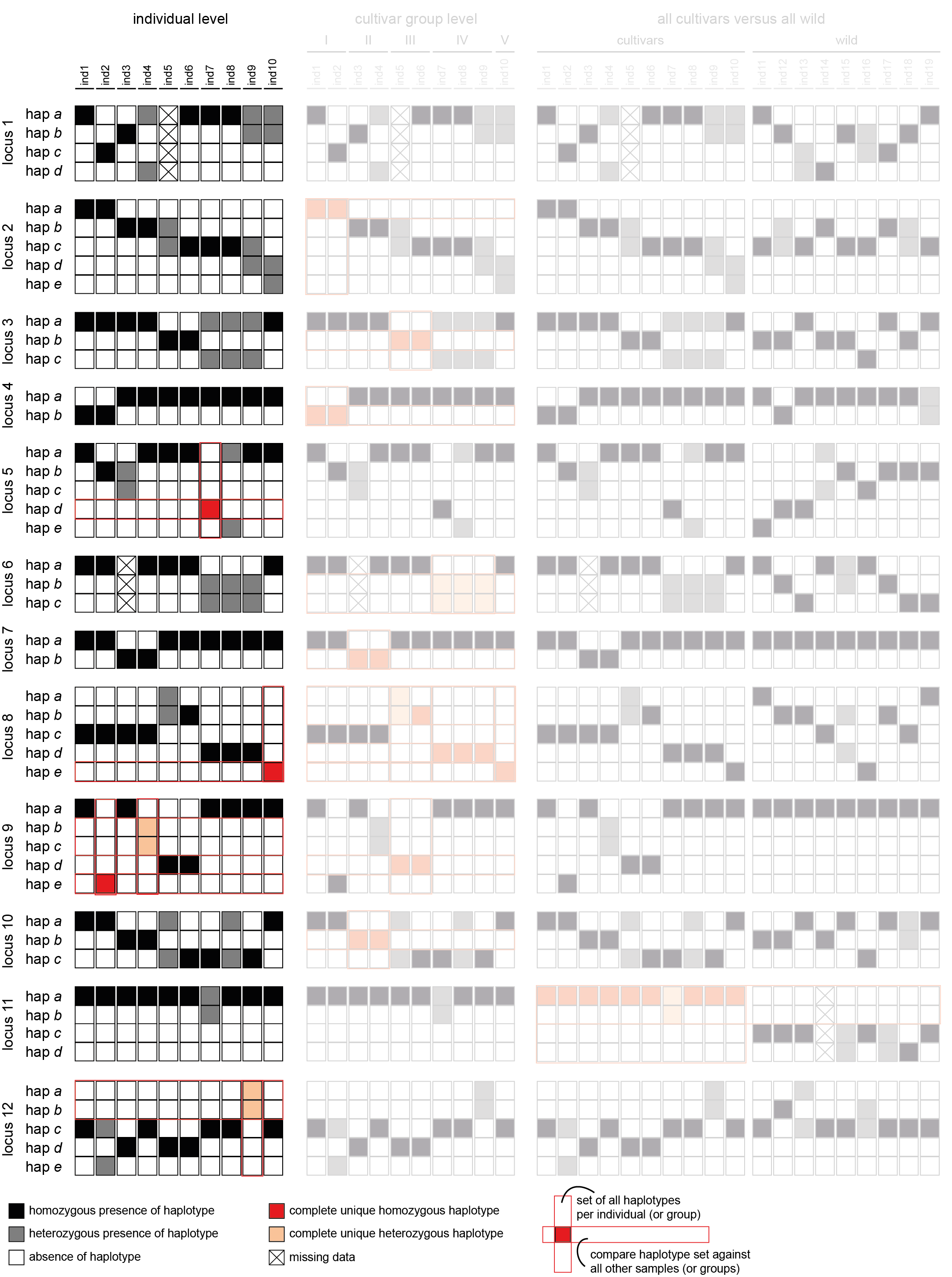
ind1
ind2
ind3
ind4
ind5
ind6
ind7
ind8
ind9
ind10
ind1
1.0
ind2
0.5625
1.0
ind3
0.21052631578947367
0.2
1.0
ind4
0.3684210526315789
0.22727272727272727
0.3888888888888889
1.0
ind5
0.25
0.18181818181818182
0.2
0.23809523809523808
1.0
ind6
0.2631578947368421
0.13636363636363635
0.15
0.23809523809523808
0.7857142857142857
1.0
ind7
0.2857142857142857
0.16666666666666666
0.19047619047619047
0.20833333333333334
0.21739130434782608
0.2857142857142857
1.0
ind8
0.4
0.20833333333333334
0.18181818181818182
0.25
0.3181818181818182
0.3333333333333333
0.7222222222222222
1.0
ind9
0.2608695652173913
0.1111111111111111
0.22727272727272727
0.19230769230769232
0.2608695652173913
0.3181818181818182
0.6
0.65
1.0
ind10
0.5294117647058824
0.2857142857142857
0.25
0.3333333333333333
0.3
0.3
0.3181818181818182
0.42857142857142855
0.4090909090909091
1.0
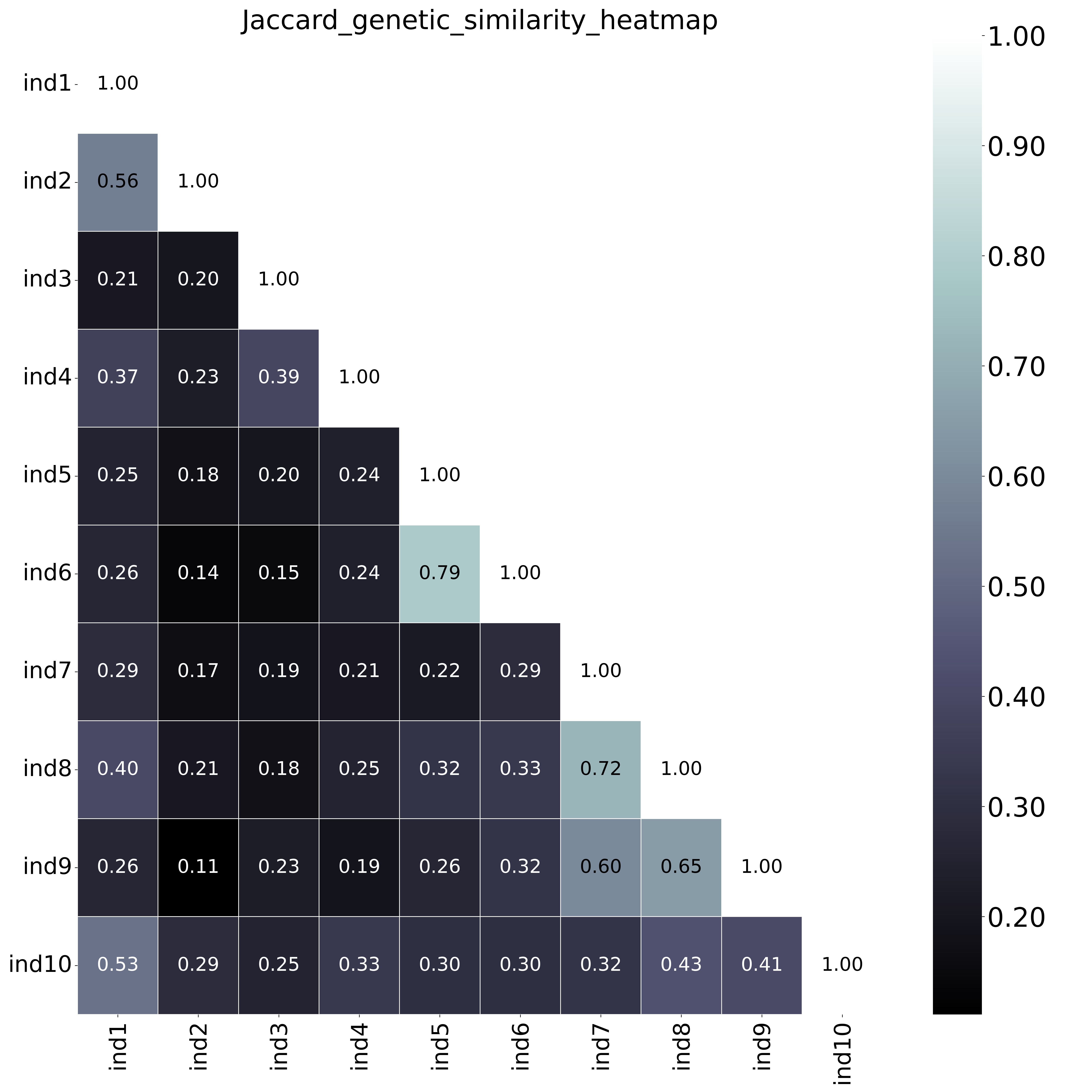 The font name and size of different elements in the graphs are changed with options
--font,--title_fontsize,--label_fontsize,--tick_fontsize, and--legend_fontsize. The legend position and resolution of the plot are adjusted with the options--legend_positionand--plot_resolution. Customize the colour scale in the matrices with the option--colour_map. Use option--maskto mask one half of the matrix (either all elements above the main diagonal or all elements below the main diagonal).
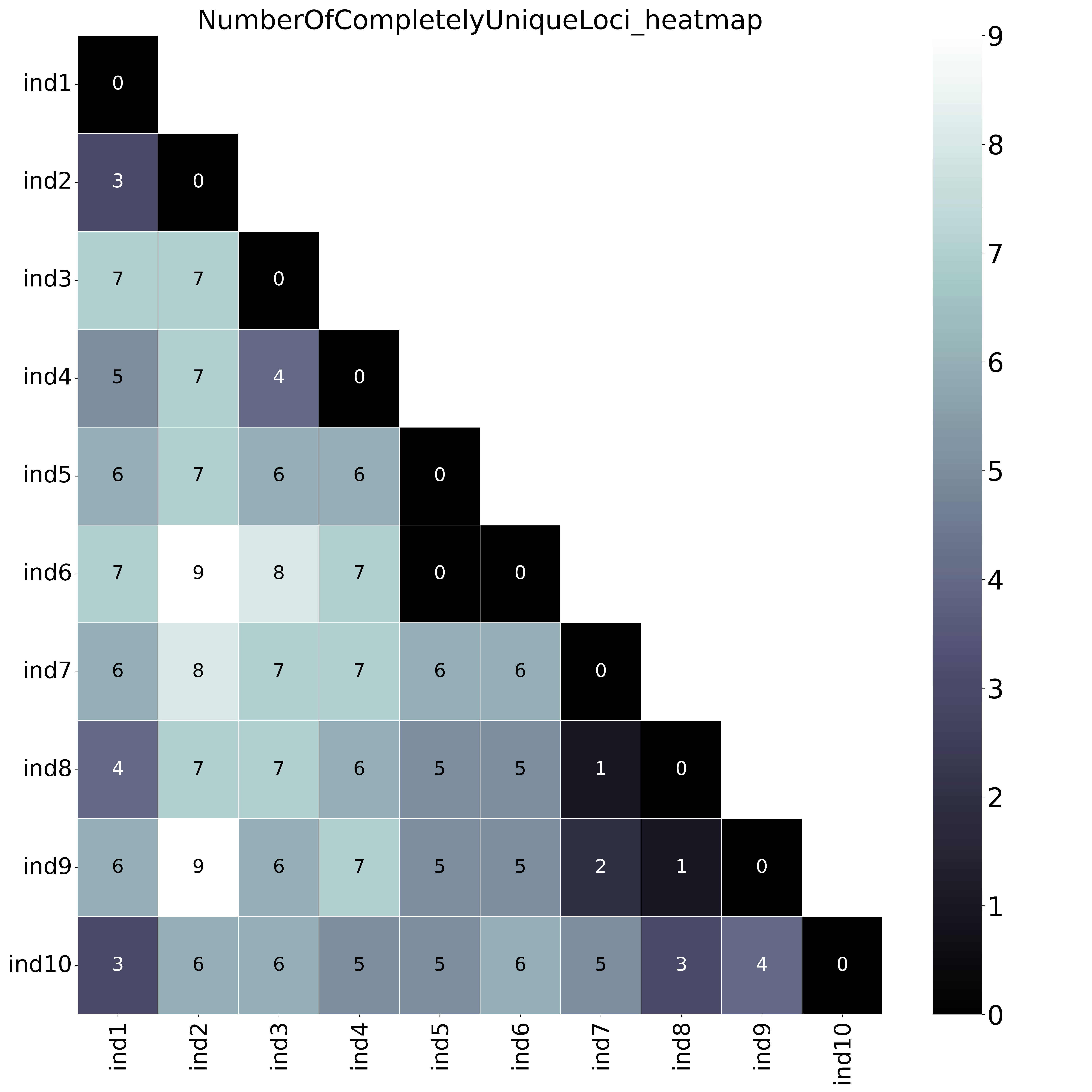
--locus_information_criterion unique.This table (NumberOfCompletelyUniqueLoci.txt) shows the (absolute) number of loci with complete unique haplotypes per sample pair, in a matrix of all pairwise comparisons.
ind1
ind2
ind3
ind4
ind5
ind6
ind7
ind8
ind9
ind10
ind1
0
ind2
3
0
ind3
7
7
0
ind4
5
7
4
0
ind5
6
7
6
6
0
ind6
7
9
8
7
0
0
ind7
6
8
7
7
6
6
0
ind8
4
7
7
6
5
5
1
0
ind9
6
9
6
7
5
5
2
1
0
ind10
3
6
6
5
5
6
5
3
4
0
With option--proportion_informative_loci, table (ProportionOfCompletelyUniqueLoci.txt) lists the proportion of the number of shared loci per sample pair (loci with data in both samples).
ind1
ind2
ind3
ind4
ind5
ind6
ind7
ind8
ind9
ind10
ind1
0.0
ind2
0.25
0.0
ind3
0.6363636363636364
0.6363636363636364
0.0
ind4
0.4166666666666667
0.5833333333333334
0.36363636363636365
0.0
ind5
0.5454545454545454
0.6363636363636364
0.6
0.5454545454545454
0.0
ind6
0.5833333333333334
0.75
0.7272727272727273
0.5833333333333334
0.0
0.0
ind7
0.5
0.6666666666666666
0.6363636363636364
0.5833333333333334
0.5454545454545454
0.5
0.0
ind8
0.3333333333333333
0.5833333333333334
0.6363636363636364
0.5
0.45454545454545453
0.4166666666666667
0.08333333333333333
0.0
ind9
0.5
0.75
0.5454545454545454
0.5833333333333334
0.45454545454545453
0.4166666666666667
0.16666666666666666
0.08333333333333333
0.0
ind10
0.25
0.5
0.5454545454545454
0.4166666666666667
0.45454545454545453
0.5
0.4166666666666667
0.25
0.3333333333333333
0.0
 With option
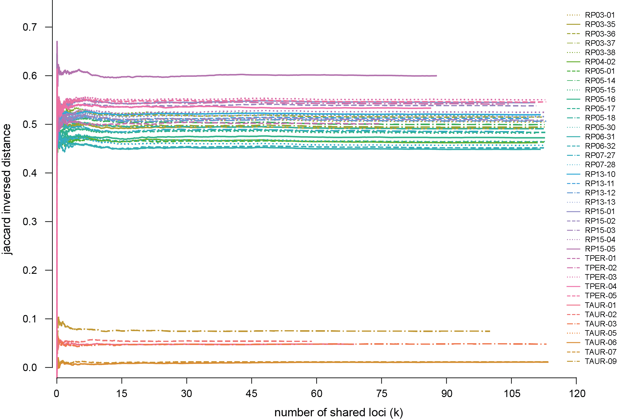
--proportion_informative_loci, table (ProportionOfCompletelyUniqueLoci.txt) lists the proportion of the number of shared loci per sample pair (loci with data in both samples).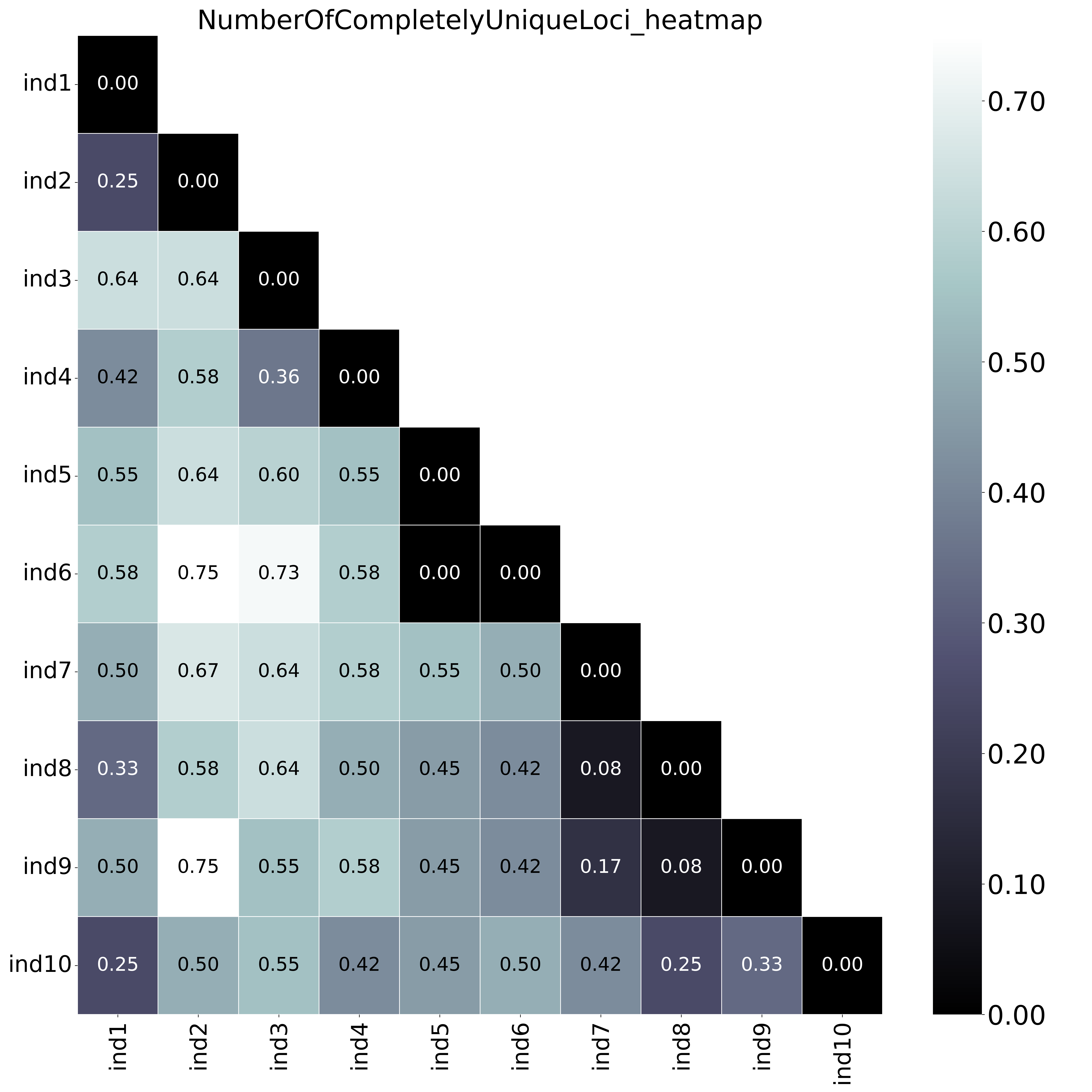 The font name and size of different elements in the graphs are changed with options
--font,--title_fontsize,--label_fontsize,--tick_fontsize, and--legend_fontsize. The legend position and resolution of the plot are adjusted with the options--legend_positionand--plot_resolution. Customize the colour scale in the matrices with the option--colour_map. Use option--maskto mask one half of the matrix (either all elements above the main diagonal or all elements below the main diagonal).This table (NumberOfSharedLoci.txt) shows the number of loci with data in both samples per pair.
ind1
ind2
ind3
ind4
ind5
ind6
ind7
ind8
ind9
ind10
ind1
12
ind2
12
12
ind3
11
11
11
ind4
12
12
11
12
ind5
11
11
10
11
11
ind6
12
12
11
12
11
12
ind7
12
12
11
12
11
12
12
ind8
12
12
11
12
11
12
12
12
ind9
12
12
11
12
11
12
12
12
12
ind10
12
12
11
12
11
12
12
12
12
12
This table (CompletelyUniqueLoci.txt) shows a list of all loci included in the analyses, the total number of sample pairs for which the loci were considered, the number of sample pairs for which the loci were informative, and the proportion of sample pairs for which the loci were informative. If the
--locus_information_criterionis set to ‘unique’, the names of samples with a unique haplotype for the corresponding locus across all sample pairs are also listed in this file (last column).
Locus_ID
NumberOfComparisons
NumberOfComparisonsWithUniqueLocus
ProportionOfComparisonsWithUniqueLocus
SamplesWithUniqueHaplotypes
locus1
36
13
0.36
locus2
45
30
0.67
locus3
45
16
0.36
locus4
45
16
0.36
locus5
45
23
0.51
ind7
locus6
36
18
0.5
locus7
45
16
0.36
locus8
45
35
0.78
ind10
locus9
45
29
0.64
ind2, ind4
locus10
45
25
0.56
locus11
45
0
0.0
locus12
45
27
0.6
ind9