How It Works
Here, we describe the technical implementation of SMAP effect-prediction.
Preparing input files with SMAP design and SMAP haplotype-window
SMAP design
During the SMAP design workflow, SMAP target-selection first selects one or more genes with a short flanking upstream and downstream region, and a GFF file is created with the positional information of the exons that together make up the protein coding sequence (CDS). Importantly, SMAP target-selection makes sure that all sequences are oriented in the direction of the protein coding gene. Genes encoded on the - strand in the reference genome sequence are reverse complemented, and all coordinates of the CDS are automatically reversed. If custom created FASTA and GFF files are provided to SMAP effect-prediction, and CDS features are positioned on the - strand in the GFF file with the structural gene annotation, SMAP effect-prediction will indicate which genes have errors, and should be reverse completented prior to running SMAP haplotype-window and SMAP effect-prediction. If the CDS of a particular gene does not begin with a START codon (ATG), or end with a STOP codon (TAA, TAG or TGA), SMAP effect-prediction will indicate which genes have errors that should be corrected in the reference sequence FASTA file or the structural gene annotation GFF file.
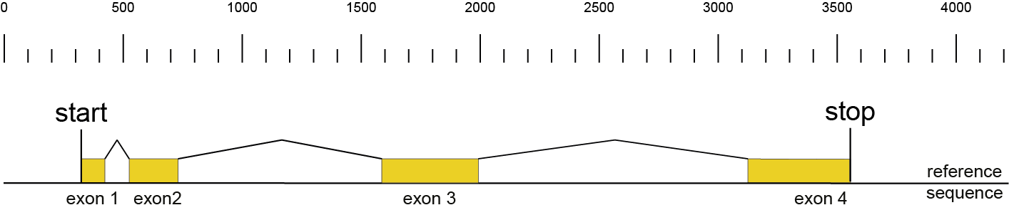
Then, SMAP design identifies amplicons and gRNAs in the CDS of the gene. One or more amplicons may be designed per gene, each containing one or more gRNAs. A minimal spacing between the gRNA(s) and the primer binding sites are respected to allow for editing at some distance from the PAM site without affecting the primer binding sites, thus retaining the capacity to amplify the genomic region containing induced mutations.
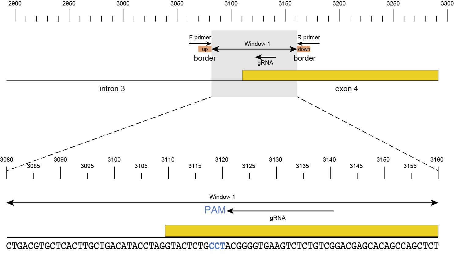
The coordinates of gRNAs and primers with respect to the selected reference gene sequence are listed in GFF files for downstream analysis. Border sequences are defined as the last 10 nucleotides at the 3’ end of the forward and reverse primers for delineation of haplotype sequences by SMAP haplotype-window.
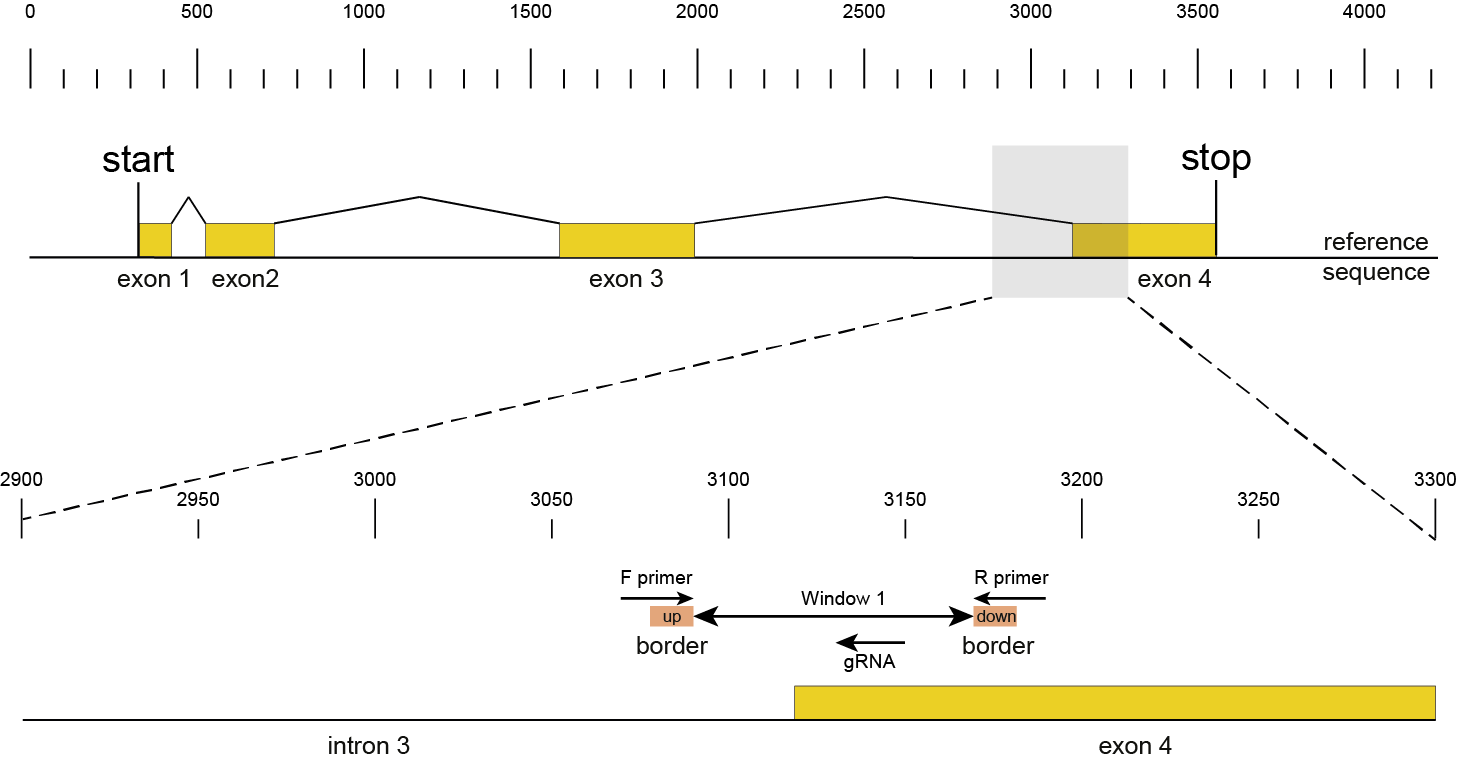
The sequences of the gRNAs are used to synthesize gRNAs and clone into expression vectors to drive CRISPR/Cas in plant materials. The primers are used for HiPlex sequencing of potentially edited lines.
SMAP haplotype-window
SMAP haplotype-window analyses reads aligned to the target loci and extracts the exact DNA sequence inbetween the upstream and downstream border sequences per locus, thus listing all observed haplotypes per locus across a collection of potential mutants. SMAP haplotype-window also calculates relative haplotype frequency per locus per sample. This genotyping table is the input for SMAP effect-prediction.
The subsequent steps of SMAP effect-prediction
Next, we describe the seven subsequent steps of SMAP effect-prediction.
Step 1. Collect
Collect all positional and sequence information needed to predict the encoded protein for each haplotype
SMAP effect-prediction collects the following information from files prepared by the other modules of SMAP:
the gene sequence from the reference genome; SMAP target-selection extracts the gene sequence and places it with the CDS on the + strand orientation in the reference FASTA file used for SMAP.
the position of the CDS regions in the reference sequence; SMAP target-selection calculates the correct positions of the CDS with respect to the extracted gene reference sequence of 1).
the position of the amplicon(s) in the gene reference sequence; SMAP design creates pairs of primers for HiPlex sequencing of genomic DNA, and stores the relative position of the corresponding border regions in a GFF file.
the position of gRNA(s) for CRISPR/Cas genome editing within an amplicon; SMAP design optionally creates one or more gRNAs per amplicon to induce mutations in a particular position of the reference genome.
the collection of haplotypes per locus and their relative frequencies per sample; SMAP haplotype-window extracts haplotypes (exact DNA sequences) using the exact same reference gene coordinates as outlined in 1)-4).
>gene1 |
ATGGGCTCCTCCTACGACCCCTACCCGTCCCCGGGCGCCGACGACCTCTTCCTCTACCTCTCCGACCTCGGCCCCGCCTCGCCCTCCGCGTACCTCGACCTCCCACCCACCCCGCAGCCTCAGCCATACCCGCAGTCCCAGCAGCAGCAGCAGGGGAGCAAAGGCCCCACGCAGGACATGCTGCTCCCCTACATCTCCAGCATGCTCATGGAGGACGACATCGACGACACCTTCTTCTACGACTACCCGGACAACCCCGCGCTCCTCCAGGCGCAGCAGTCCTTCCTCGACATCCTCTCCGACGACGCCTCGTCCCCGACCACCACCACCGGCACCACCAACAGCAGCGCCAGCGTCAACCACTCCTCCTCCGACGCGTCCGCCAGCGCGCCGCCCACCCCAGCCGCGGTCGACTCCTACTCCCCGGCCCCCGCTGTCCAGTTCGACGGCTTCGACCTCGACCCCGCGGCCTTCTTCAGCAACGGGGCCAACTCCGACCTCATGAGCTCCGCCTTCCTCAAGGGCATGGAGGAGGCCAACAAGTTCCTGCCCTCGCAGGACAAGCTCGTCATCGACCTCGATCCGCCAGACGACACCAAGCGGTTTGTCCTCCCCACCCGCGCCGCAGAAAACCTCGCGCCCGGATTCAACGCCGCCGCCACCACCGTCCCTGCCGCCGTGGCTATGGCGGTGAAGGAGGAGGAGGTGATCCTCGCTGCGCTTGATGCCGCGCTTGGCAGCGGCGGCGTCGTCCTGGGCCGCGGTCGGAGGAACCGCTTGGACGATGACGAGGAGGACCTGGAGCTGCAGCGCCGGAGCACCAAGCAGAGCGCGCTGCAGGGGGACGGCGACGAGCGGGACGTCTTCGAGAAGTACATCATGACCTGCCCCGAGACGTGCACGGAGCAGATGCAGCAGCTGCGGATCGCCATGCAGGAGGAGGCCGCCAAGGAGGCGGCGGTCGCCGCCGGGAACGGCAAGGCCAAGGGCCGCCGCGGTGGGCGGGAGGTGGTGGACCTGCGCACGCTGCTCGTCCACTGCGCGCAGGCCGTCGCCTCGGACGACCGCCGCAGCGCCACCGAGCTGCTCAGGCAGATCAAGCAGCACGCAAGCCCGCAGGGGGACGCCACCCAGCGCCTCGCTCACTGCTTCGCCGAGGGCCTCCAGGCCCGCCTCGCCGGCACCGGCAGCATGGTTTACCAGTCGCTCATGGCCAAGCGCACGTCCGCAGCCGACATACTCCAGGCGTACCAGCTGTACATGGCCGCCATCTGCTTCAAGAGAGTCGTCTTCGTGTTCTCGAATAACACCATCTACAATGCCGCTCTGGGCAAGATGAAGATACATATCGTCGATTACGGGATCCATTACGGCTTCCAGTGGCCGTGCTTCCTTCGATGGATAGCGGATAGGGAGGGCGGGCCACCGGAGGTGAGGATTACTGGCATTGACCTGCCCCAGCCTGGGTTCCGCCCTACTCAGCGCATTGAGGAGACAGGGCGCCGGCTCAGCAAGTATGCCCAGCAGTTTGGTGTGCCATTCAAGTACCAGGCGATTGCAGCATCCAAGATGGAGTCCATCCGCGCGGAGGATCTGAATCTCGATCCAGAGGAGGTGCTCATCGTGAACTGCCTATACCAGTTTAAGAACTTGATGGATGAGAGCGTTGTGATTGAAAGCCCAAGGGACATTGTGCTCAATAACATCAGAAAGATGCGGCCTCATACATTCATACATGCAATTGTGAATGGCTCCTTCAGTGCGCCCTTCTTCGTGACGAGGTTCCGAGAGGCTCTGTTCTTTTACTCGGCCCTGTTTGACGCTCTGGACACGACCACTCCAAGAGACAGCAACCAGAGGATGCTGATTGAGGAGAACCTTTTCGGGCGGGCTGCCCTGAATGTCATCGCGTGCGAGGGCACAGATCGGGTGGAGCGCCCTGAGACGTACAAGCAATGGCAGGTGCGGAATCAACGAGCAGGCTTGAAGCAGCAGCCGCTGAACCCTGATGTCGTGCAGGTAGTGCGGAACAAGGTCAGGGATTTATACCACAAGGACTTTGTGATCGATATTGATCACCACTGGCTCTTGCAGGGATGGAAAGGCCGCATCCTCTATGCCATCTCGACATGGGTGGCAAATGATGCCCCCTCTTACTTTTAGCTGTTTTTTTGTGACTCACTTGTCTACAACTTTAGGGGCCAGTTTGGTACGGCGCGTGCGGCGCCACGGCGCGCCTAAGCTGCGGCGCCCGAATCGGCCGCCACACCTGCGGCGGGAAAACTATGGCGCGCCGTGGCGGCTTAGTCCACGCACCAAACAACCCCTAGGTTTAGGTATGTCATCTAGATATATCTAGTGACAAGCGTGTTCTTGGCCCAGTTAATAGCCATGGTTACTTGGACTCTGCAGTATGCCTAGTGCCCTAGTGAGAATTCAACATGTACCTGTTCTTTCCAAGGGTACATTCAGCTTCTGTGGAACATGAGTGACACACGGGGGATCCAGAAGTCAGAAGGCATACCGAAATCTGTCCTTTGATTTAATGTGGATTATATAGATGCTCATCACTCAGTCATGCTGTTGCATGGTGCTAAATATGATCTAGATCTAGGTCCTGGTCTGGATAATGCTCTCCACAGCATCTGCTGTGCGTGTGACCTGTGATCAGTTCAGTCAGTTGATCAGGTTGTAAATGACACTTGTTCCTCTGTTTCCGGCGCTTACTGCGCTGTTTCAGACTTAACCATGGCTATTATGAAGAGATGAAGCGTGGGTTTTTTTTGTCTGTCTACTTTATCGCATATGGGGGAGCTCTTTCCAGGATTTATATGCCATGTGTTTGTTCATGTACATGATTCATGTTCAATGAGTTGAATCCTCTTTCCAGCCTGCATACTGGTTTGTCGCGGCGAGGAAATTATTATTATGACAGTTTATGAACTGTGGCTGATGAATTGTTCAGTAATCAGTCGTGCTGTTTGGTTCACGAAATGTAACGTAAATTGTAACGGTAATGATTCACATTCGATTCGAGTACCAGTGGTAACAAATTTGAATATGCCGATATTAGTTCTTAGTGTGATTTAGTTTCTAGTGTGATATTTAATTACGGTTGGTCACAAACAAACATGATATAACGTTATTAGTTATCCATTACGTTACAAATATGTGAGCTAAACGACACCTTATTAGGCTGTTATTACCAGGATTGCAATTATCTCTTGCTGTACTGTCTCTGCGTTTTCAGGCTACATATGGGGTTTTGTGAGGCCCATGTTGTCTTGGTATGGGAGCTCTCTCCAGCCGGTGCGCATGATTAATCGGTTCATGTTCAATTAAATCCAATGTTTTTTGGCCAATATGTTGATCCAGTAAAGGAAATAGATGATAGACAACCCCCTGGACCATCTAATTATTGTTTTTCTATCTCTCTTTTTATAAGCCATTGATAAGATCAGAAAAGAATTTTTTTTGACGTGGTAGAAAGGAGAGAAAGGGAGGTCTTCTAACTTGGATGTCGCGGTGTTATCATTGGGTGTCTGTTTCGGTCTTTTTTCAACTTCTGGTCATGAAGTTGTTGTAGACTGATAAACGTCTAGCTTTTAAGTCTATTTTTGAGATAATTGTTTAAGTGAGAACAGTCTAAAATGAACACAAAATTTATTAAATCATCGCGACAATAGAATACATTATTTTTTAGGTCCTAAACCCTATAAAGTCCCTCAATTTTCTCACCACATAATTCCCATTATACTTAGATTTTCCTCACAATCAGATTTTTAAAAAAGCTTGTAAAAAAACTGAAACAAACAAGCCAATAGTGTTCAAGAGCACAGTTCGGTCCCCTCGTGATGAGGTGGTTATGGCTGGCCAAAACATCCGGCTTTGGGCCCCCCTACCTATTCAAGTCTTGTTCCATCTATCTCATGTGGATGGAAAGAGATTGAAAAAATTATAAAATATTTTGGTTTGCTTGAAATTTAAATTTATATGGATTGAGAACAAAACGAACGAACCCTCACATGGCAGATAAAATCAGTGCCTTTTCCCCCTCCATGGCAGCTGTCTGTACTGAAGCTTTGTTCCGCTGTGACCGATGGCTGCAGTTTCAAAGCGAAGATTTAAAAAAGAGGACGGTGCAAGAAGCTCTTCTAGGCAGAAGTTGGAACTTTAACAGCGGATGCCTTGAACAGCTTGGAATTACAGCCGGGATATTGTCCAGCGATCACTGATCAGGCGACACCTTTCATCAGGATGATTTGCTGATGTACAAACAGACAGACAAACAAGTGTGTTCTCATGGTCAATGTGCTTACGACTGACCATCCACTGCTTTCGCTTGCCACCAGTTCACCCTTTTCCGCACGTTTGTAATCGCGCGCGCGCGAGAGAGAGAGGCAGTGTACGGCTTGTCTTCCTCAGTTCTCACGTTTGCAATAGCGTTACCCCTGCACCTCTCTCTGCTGAATTGTTGAGCAAGACATCGGCACCTCCAATCAGGAGGAGATTTGTGATGCTTCCATGTCGTGA |
>gene2 |
GAATTCCCGTGCCGGTGGGGCCGTCGGCGACGCCATGTGTCGCCGCGCTATCGCCTGGGTCACACAAGTGTGCGGGTGGGTGGCCGCCACACGCTCGCTGCGCCTGCGTGCGTGTGCTCGCCTCCCACCCTCCCCGCACTAGCTCTGCACTTTCCCTGGCAGTCGTCCCTTGTTCCTGACTTCCTGCCTGAGCGCATCCGGCCACCTTCTATCCGCCCGCCAGTCCCCGCCGGCCTCCGCGGATCATCTGCCTGGGATCAAGATCCGTCGAGGCCGAGGCACCCGCGCGCCAAAGATCGTTTCTTGATCTAAATTTGGGTGGTCGTAGGGATCAAAGCTCGGTTCTCTGCGGTGCAGTTGAGAGGGGTAAAAGTTGACTCTGATTTGTTGAGGTGTCTGGGTGTGAGAGTCGGATGGGTTCTGTGTGAAAGCTGGTGTCTCTATAGTAGTTCGAAAGGTTGAGCAATTTGGTTTAGATACTGTGGCGAGGGAGAAGGAAGATGGTTTCTTGGTCAGGGGGGGCTTTAGCCTGTAGGGTTAGGGAGTAGTGCTGTTCATCTTATCTATGCTCTGTGTGCTGTTAAATATCTGAATTGGATTCTTTGTGTATTTTCCAATGAGAATAGTTAGTTGCATTATTTGCTCTCAATATAAGAAGGACGATAAGCCTTTGATCTAAAATATAATAATTACTTGGATCAAATTGGCTTTAGTTTCTTGATGGGTTGTATGACAGCATGTGCAGTTTAAGATTTTTGCTGTTGTTGTGAGGTAAAGAGAAAGAATAGCTAGCTTGATATGACTTCTTGGACTGTTCATAGTGTTCTTGTGTTGTTGGATTTGAAAGGCTGGCTAATTTGGTAGGTTAATATAGCAACCAGTAGTTATAACATAATTTTTATTTGCAAGATTAGAAAATTGTATTGAGTTCTTGATGCAGATTCAAATAGACTTTTTATTGCTGGTTTGATCCTTGTCCATAGTCCACACATAAAGTTGATTTTTTATCTAATTATCTGCACTTCATGATCTCAATCAAACATATGGTGCTTCTTGTTCATATTTCTTTTTCCAGCGAGGTTAAAAGTTTAGCTCGTTGTGGTATTGTGATTTGTGAGCAATTGATGCTTCCATGGTACAGCATCCTAAGGAACTCCATATTTTTATGTGGACTGTATTTGTGTTCTAAATTGTGATACCTTGCGGCTCAGATTAGTTGCCCTTTGTTGCTACACATGTTTTTAACTCTTTTGATTCTTAAATATTCAATTTTGTGATGCAGCACCAATATTCTTGGCATGGTGGCTGACACGGAAAGCTCAGATTCACTGCCTGGCAGTTCAAATGCTGCTTCTGAGATGCCTGCTAATGGGTTAGCCTCAAAATATTTTTTTGGATCCAGTTTTGTACAACTAATTTCATAGCAGTAATCAGTATTCACTACTACATCTGCTCTTAGTTAGCTACCTATATTGGGTGTACATAAAAATGCTAGCATCCACAGTCCACCAGATGATTATTATGTCCCCAACCTCTTCATTTCATCCACTGCAAGTAATAAGATCTGACCAAAATGAGCAGAGCAAAATTTAAGGTAGACTGTGATCTTGGAATAGATGTTGTAGAAGATACAGAAATATGATTTAACCAGTAGTTTATGGCTGAATCCTCTTTATTTGCATTCGTTCCTCTTGTTCAGTTTAATTCTTATCTTCACCTTTTTGGGGTTTTTTGGCTAATCATTTTGCTGCTTGTTCAGTTTCATGTCATATTGAGTTCTTTAATAGGCCAGTAAAGGGCCATAACTTACTTAAAGTTTATGATCGTTGAGAGAGACAGAGGAGGCTATATGCTATTAATAATCACTACCTCTACCTCATAATTAAAGCAGTGTCATCTGCTCCCATAGGCATATCAGTTTCACCTGCATGAATATAAAATCTAAGACTAGCCATCAATTCAAATGGTATGAAATCGCAGGAAGTTCTGGCTCTGTTTTCTTTTTTTTTCTTGGGTCTTAATTTCTGACCTCACAAAAAAAATGGACATAGAAAGTTTGCTATATATAAAACACAACCTCCATATATATACATTAAAATTACTAGAAGAAACCCTTGAGAACTAAAGAGTAAAGATTGTTTAGGACAAGAGCTGTGCAGATGGGTTCCGGTTCCTAAATCCTGTGTAGGACCTCTGTGACTGAGGCAGTCATAGAAAAGGTTTACAGTTAGGCACTTCCCACTCGCCACATTAGAATAAGGCCTATAGTTCATAGTTGTTAAGTGTTAACAGAATCCTAGTGCATTAAATTTCAATTAACTTAAATTAATATGTGTTGTTGTAGTAATTTGCACGCTATCGACACACAGTATATGTTTTGTTCAAAGTCTATATTTAGATACCTAGGGGTAAGGCTTGCCTCGGTTATTCATCCCCTAGACCCCACTTAGGGCATGGTCGGTTTAATTCCAATCCATGTGGATTGTATGGGATTGAGTGTGATTAAATCCCAAACAAATCAAAATCTCTCATAATTTATTTCAATCACAATCAATCCATATGGGATGAGAATAATCGAATAAGGCCTTATGTGGGAGGCCTAAGCACTGGCTCTATCCTGACCTAGGGGAGTTAAGATTTCCCTAGTCTTAGTTGACCTATTTTTACATTTGCACCTTCAGATTGTTCTGAATAATGACGCTGTCTATTCTTTCTAATACATATTTGCTCTTGTAGTGTGCTCCCTCAGCCTACTCGCCTTTTTTCCCGCTGCACTATTTTCCTGTTTTCTGAACAATTTTCCGCTGCAGGTCTATTCACCGAAAGTCTCAGGAAAAGCCCCCCAAAAAAACACATAAAGCTGAACGAGAGAAGCTTAAACGTGATCAGTTGAATGACCTTTTTGTTGAGCTCGGCAGTATGCTAGGTTAGTACAGTAGGTCATTAACCATTGACTATATGTAATAGACACAATTACGCTCTTGAGAAAGATATCGGTATCTGCGGTTAGATTCCATCATTCTGTTCTCCACTTGAGCTCATCTGGTAGACCGTTTTCAGCAGTTCGCCTATATGGTCACCTAAAACACCGTTTTTCACTGTAGAGTGGAGTTTGAATATAGATATGAAGATGAGTAAGCTGCTGAAAATAGCCTTAATAGTGGTTAGCATGATGTGACCTCTCAGTGGGGACTGAAATTATAACATACATTAGCTTATAAGTTGTTTACAGGATCCAGTACATAGTATATCTGCATCATTTTATATATTAGGGCGTGTGTGGTTCCCAGGCAGCTTTGCCTATTAGGCATCAATCTCAAGTTGTTGATTTTGGTTGCTTGGTGGACAGGATCGCTGCCTGGCAGATCGTGAACCATTTCTTCTGATTACGTCTATGGTTGTTGCCATGAAAAGAACTGCTAATCTCTCTACAAAATTCTTCAAAATTAATGTATGGTTAAGCTATTAATACTACGCTGTACTTTGAATGGAACACCATTGTGGATAGTTCTTGCTGATGTACCATGCAATCATGTTATTCTGATGACATAGGGATTGTCATCTGCTGAACTGCGTACTTATGATGAACACTGATGTTTTTTCTTTGTATTCTGTGCCATTAAATATGATTGCATAGTCATCCTCATATGTTCCTGTTGCTGGTTATCGATTTTGCTACAGATGTCTAAGCCATTGATCAACATAGTTCTGCCATTACAGATCTTGATCGACAAAACACTGGAAAGGCTACAGTGCTAGGTGATGCTGCGCGAGTACTGCGAGATCTAATCACTCAAGTGGAATCTCTCAGGCAGGAACAATCTGCTCTTGTATCGGAGCGCCAATATGTGAGTTTCCAAACTGAAGCACTTATGTTATGTACTCTTCATAAAAAAAAAAGATCAGCGTGATATATTCTGCATGAATTCTGATGTTTCTCAACTGATATACCACCAGATCCTCTACAGTCACCACTTGCCTTGTTCAGAAATATAAACATCTAGCTTGAGTTGATCCTCTAAAAGTAGGACACATTACCTGTTGTGAATCCTGTGACTGGTTCATTGAAACTGACCGTGGATGCGAAACTCAACTGATATATTCAATTGACTCTCGTCACCCGTTTCATATTCACTGCTCGCTTGATTTAGTTCTTTGGTAGATGTTTCAGCTTACTATCTACTAGTACCTGTTAAGCCTAAAGCACACTCTCATGGACAGGTCAGTTCCGAGAAGAATGAGCTGCAAGAGGAGAACAGTTCGCTCAAGTCCCAAATATCGGAACTACAAACCGAGCTCTGCGCAAGGATGAGGAGCAGCAGCCTGAGCCAAACCAGCATCGGGATGTCGGATCCGGCAACTCACCAGCAGATGCAGATGTGGAGCAGCATTCCCCACTTAAGCTCCGTGGCCATGGCGGCGCGCCCAGCAAGTGCAGCGTCCCCGTTGCACGGCCAGGAGGGCTACTCTGCTGACGCCGGTCAAGCGGGCTACGCGCCGCAGCCGCAACCTCGGGAGCTGCAGCTCTTTCCGGGGTCATCGGCATCGTCTTCACCGGAGCGTGAACGTTCTTCCCGGCTCGGAAGCGGCCAGGCCACGCCGCCGAGCCTGACAGATTCCTTGCCGGGTCAGCTCTGCCTGAGCCTCCTACAGCCATCTCAGGAAGCAAGCGGCGGCGGCGGCGGCGGCGTCATGTCGCGCAGCAGAGAGGAACGGCGGGACGGG |
>gene3 |
CTGCCCTGCGCGGCTGCGGTCGCCTATAAGGCTAGCCCAGGCCATTTGCCCTTTGCCCCCGTCCGTCCGTCCCTCACCTCACCTCACCTCACCTCGGCCCGCCTCCCTCATCAGGTAGCCGTAGCGAGCAGTATAGCACGCACAGCCGCCGCCCTGCCCTGCCCTGCCCTGCTCGGCGTAGGCACAGGCACAGCCCAGAGCGAGCGAGACAGAGGGAAAGAGACAGAGCCAGCCAGGTAAAAGGCAAAAGCACAGCACATTAAAAGAGAGGCCGGAAGCAGCGGCAGAGCGGAGAGAGAGAGAGAACTAGAAGCATATATGGCGATGCCCTTTGCCTCCCTGTCTCCGGCAGCCGACCACCGCCCCTCCTCCCTCCTCCCCTACTGCCGCGCCGCCCCTCTCTCCGCGTAAGCCACCTCCCTTTCGCCCGTCCGGGAAAAAACCCTCTTCTTCGCTCGGTTTATGCCACCCGGAGCCGTGCTGCAGCCTGCAGGTATCTGATGCCGCGAGCTTTGCCTTGCAGGGTGGGAGAGGACGCCGCCGCGCAGGCGCAACAGCAGCAGCAGCACGCTATGAGCGGCAGGTGGGCAGCGAGGCCGCCGGCGCTCTTCACCGCGGCGCAGTACGAGGAGCTGGAGCACCAGGCGCTTATATACAAGTACCTCGTCGCCGGCGTGCCCGTCCCGCCGGACCTCCTCCTCCCCCTACGCCGAGGCTTCGTCTACCACCAACCCGCCCGTAAGCAAGCACGGCCCCCGCGCCGCCTCCGCACCCCTTCACACTCACACGCACGTTTAACCGCTTTTGCACTGCACAACCCCGGCCGCCCGGCGGCGGCGTCCGTGCCTTGATCTGGTTGTTTACTCGGATCGAGGGATTCAGATGTCCTCTCCGTCCGTTTGTTAATCGGCTCCGGTCATTTCTTAATCTCGTCCTGGATTCGGTCACGAAAAGCTAGAGGTCAAGATTTTGCTCTCGATTACTATATCCTTGCCTCATGTTCTAATGGAGTTTATTTTATTGGTCTGATGTGATTAGATAGGATGCTAGCCAGGCTTGTCTCCGGCCAAAAGCGGCGGTTTAGTTTATTGATGATTGCTTCTTTCCTTGGGGGATTTATTCCTGTCTGGTTGTTGGGAGCCTAACCACGCTCCTATTGCTGCTGCGGTTTACTAACCATCTGCGCCAGTACACCTACTCCATGGACCCCAAAATACAGTTCTTCCAACCATTCCCCCCCTCCATCTGCTTTCTCGCGGGCAAATAAAAACGTGTAGAACGACGGTGTAGTAGGCAGATCTACTCCTTGTGCCGCTACGCTAGCCCGCTACCGAAGATCGGGCCCGTTTCAACCGGTTCGTTGGTCTGAGCGGAGCTAAGATGGGGCGCATTTCATTTTTTGGTCCTTTCGTCTGATTGGAGAAGTGCCCATTCCGGTATCGCTCCCCGGCCTCCAAATACGCACCGACACAGAACGTGTTCGTACGCACGTACACATGGTATGCGCACCGTGCTGCTGGCCATAGCCGTTGACTCACCGGGATTCACTCCTCTCTCGCGTGTGTGTGTGTGGCTTCCTTGCAGTTGGGTACGGGCCCTACTTCGGCAAGAAGGTGGACCCGGAGCCCGGGCGGTGCCGGCGTACGGACGGCAAGAAGTGGCGGTGCTCCAAGGAGGCCGCCCCGGACTCCAAGTACTGCGAGCGCCACATGCACCGCGGCCGCAACCGTTCAAGAAAGCCTGTGGAAGCGCAGCTCGTGCCCCCGCCGCACGCCCAGCAGCAGCAGCAGCAGCAGGCCCCCGCGCCCACCGCTGGCTTCCAGAGCCACCCCATGTACCCATCCATCCTCGCCGGCAACGGCGGCGGCGGCGGCGGGGTAGGTGGTGGTGCTGGTGGCGGTGGCACGTTCGGCCTGGGGCCCACCTCTCAGCTGCACATGGACAGTGCCGCTGCTTACGCGACTGCTGCTGGTGGAGGGAGCAAAGATCTCAGGTGAGCTTCATTATGTTTTCTCTGCAACCTCTGTCACGTATCCCACTGTTTAGTCCTAGCACATGGCGTAGTTAGCTCCCTGATCGGTGTCAGATGGGTCATGGCACCCGCTCGATGGGGGGGTGAATGCATGCTAATCTGTTGTGTGATGCACTGTTCCATCATTGCGCTAGATTGCCTTTTACGCTTTGCATTCAGAGTACTGCAGACGCTAGACAGCAGTGTGGATCAGATCGACTAGCGAGTAGTGCAGCACCAGAAGCACCTTTTATTATCTGCCCCAGTCGTTATCTGAGATCTGTCATCAGGCAAAGTAGTGGTAGCGAAGAACTGAAACATCTCTCTGCCTCTGCACTCGGTACTCTGCCAAAGAAAGTAGAAACACTCACACCTCTGCTTAGCCCCTCTGTGCTCGCTTCGATCTGGTCAATTCTTTCTGGAACCTGTGATTTCTCATCCTGAGAAGATGACGCTTTCTGGTACGCCAGATCGTGATGATGGAACACATCTGGGCTCTACGTTCAGAACTAGTAGTGCCTGCATCTCTATGTTCCTGCTCTGTCGTGTACTAGACATACAACATTTATTATTATTCTTCGGACGGCTGCTGTTTTTTTCTCCTTGCGCAGAACTGCTCACAGAAAACTGGCGTGTGTTTTTTTTCTTTTTTGGCCAGAAACTTCTCATCCGTGTGCCTGGAAGGAACCTAATAAAAAATCTGAAAGTTCTAGTAGCATGATAAATTGATAGTATCCGTTGGCCGTCTCATTTTGCACGCGAAGCTTTTGTGCAGCCGTCGGCACTTTGCAAATTTACAGTGCTTTACCCAATCTCAGTCATTGTAGGGTTACCTGCAGGGCACATGGTCTACGTGTTTGCTTACATGATTGGTCTTCCCACTGTTGTTTGTTGTTTCTCTACCTTTTGTCATGAATGGCCGCATGCTTTTTCAGAGAATTCCTGCTACACAATAGCACAACCAACAATACTACTGTTTCGGCAAAACATGGTTTGCTTGCATGGTGTGGCCAAGAGTTTGTCCTCTTGTTTGCCTCGTTGGTGGGTCATGCATGTTCATCTCTAGACTGACGTGCTCACTTGCTGACATACCTAGGTACTCTGCCTACGGGGTGAAGTCTCTGTCGGACGAGCACAGCCAGCTCTTGTCCGGCGGCGGCGGCATGGACGCGTCAATGGACAACTCGTGGCGCCTGTTGCCGTCCCAAACCGCCGCCACGTTCCAGGCCACAAGCTACCCTCTGTTCGGCGCGCTGAGCGGTCTGGACGAGAGCACCATCGCCTCGCTGCCCAAGACGCAGAGGGAGCCCCTCTCCTTCTTCGGGAGCGACTTCGTGACCCCGAAGCAGGAGAACCAGACGCTGCGCCCCTTCTTCGACGAGTGGCCCAAGTCGAGGGACTCGTGGCCGGAGCTGAACGAGGACAACAGCCTCGGCTCCTCGGCCACCCAGCTCTCCATCTCCATCCCCATGGCGCCCTCCGACTTCAACACCAGCTCCAGATCGCCGAATGGAATACCGTCAAGGTAAAGCCGTCGATCCGTAGGCACACTTGTTTTTTTTTTCTTCTTTTCTTCAGGTTTGAGCCTTTCGTTCTGCGAACCTTCTTCTAAATTCCCGCACGGCCTTGCAGATGAACCTGAGTAACCATGCGGACCCCAACATCTCAGAGCTGACGACTCTTTGCTGCTGGCCTGGCCTCATCGTACCTTGAGGCGTCAAGGAATACTTCATTACCACTAGTATCATGCTCCTGGATTTTCGAACAATATATATATGCTTATGTACCGCTATTTCTCTCATCTTTTACACTTCTTTACCCGTTTGGAATTGTATGTTCTGCGTGGCACGGTTGTTCATTTGACCTTTTTGGATTTGATTGAAAGCTCCGTTTCTTGCTTACTCCAGCGCATCGTGAGCAATGTCCCTGTCTCCGCTGCATGTGAAAGAT |
>gene4 |
GAACAGTTGTGGGGCTGTGGGCATTCAATTGCTTTTGCTTCCTCCGTTCCCCCATCTTGCCATCTCCCCTTCCCCTGCTCCCCCGAAGCAGCAAGCCAGCCTGCCCACCCGCAGCCATCACCTCCGCCGCTCTCCACCATGAATCCGATCCACCAGCACGGCATCGTACCCAATCCTTCGTGACTGTTGCCTCCGCGCATCTCCGGGAGCAATGGAAGGAGGCCAAGATGTGTTCTTAGGTGCGGCGGCAAGGGCGCCGCCGCCGCCGCCGTCTTGCCCGTTTCACGGATCCGCTACCGCCACCCGCTCCGGTGGAGCGCAGATGCTCAGCTTCTCCTCCAATGGCGTAGCAGGTGAGATGTTGCAGATCTTTTCTCCTTTTCCTCTCCTTTTCATTTTCCTTTCAGTTTTTCCGTGGCGAAGATACTGTTGCATTTGTGGGGGCAGTGCTCTGTGCCTCTGTCTGAGCTGATCCCAGCTGTGATTGATTGCTTGCTCATGGGTCACGGCCATGACCATGGCATCCCCTCCTCTGCAAAAGCCCGTGCCTTTGGTGTCTTGTCACGGGCAAAAGTGGCGCATGTTCATTATTATCCCCCCTGCCTTTTTGCTTTCGCAAGCCCTGTATGTGTCCTGGCCATAAAGATGCAATCTTTATCCTCTATGCACATACTTCACCCGAAAAAAAGCTAAAGGGGTCACTGATTGGTGCTGCTTCCTTAAATCTTGCATGTGTGGGAACTAGGAGGCCATTGGTCACGGGTACTGTTCCCCCTACTGTTCTTGCTTCCCGTGTCCTGACCATTTCAGTATTCGTTCTTGTTACTGATGGTGTTCTTGTGATGAAGGGTTGGGTCTGTGCTCAGGTGCCAGCAAGATGCAGGGTGTGTTGTCGAGGGTGAGGAGGCCCTTCACTCCGACGCAGTGGATGGAGCTGGAGCACCAGGCCCTGATCTACAAGCACTTCGCTGTGAATGCCCCTGTGCCGTCCAGCTTGCTCCTCCCTATCAAAAGAAGCCTCAATCCATGGAGCAGCCTTGGCTCCAGCTCATGTAACTCTTCTCTCTACCTTTCGTTTATTTTTGTCAATACCTGAATATAAGGATAGTGAAAGTAAGACCTAAAACTGAGCAAGTAAAATGGTCAGCTAGGTGTAGATTTACTGTTGATCCAGTGCTCTGTTTCTTGTTTTGGCTTTATCTAGGATATGAGTGTTGTCATCAGTTTGTTTAATGAGACACATTGGAAAGTAACAAGCCTGCGCATAATAACAGTCTCAATGATTTACTAGTGTTAGAGACATGATTTAGATATAAAGCACTTGTTGCATTGGGATCTTGTTGTTCCTTATCTCTTGTGGAACAAGATTCAGAGTTGTCAACTTATCATCATTAGTCTGTTGTAATATAAGCACATCCAAATGCAAACTTGGCCACTTGATGATCTGATGTTTTTGTTGTTGCTGGGATACTGTTATACTAACACATTTTGGGGGTTGTTTATTGCATTCTCATTTGTAATGGGGACTCTTTTGCAGTGGGATGGGCACCATTTCGTTCCGGCTCTGCTGATGCAGAACCAGGAAGATGCCGCCGCACAGATGGCAAGAAGTGGCGGTGCTCTAGAGATGCTGTCGGGGACCAAAAATACTGTGAGCGACACATAAAACGTGGTTGCCACCGTTCAAGAAAGCATGTGGAAGGCCGAAAGGCAACACCGACCACTGCAGATCCAACCATGGCTGTTTCTGGTGGTTCATTGTTGCACAGCCATGCTGTTGCTTGGCAGCAGCAGGGCAAAAGCTCAGCTGCTAATGTGACTGATCCATTCTCACTAGGGTCCAACAGGTGAAGTCACCTGATCGTCTGATCCTGCATTGTTATACTCATTTCTGCCACTTAAGTTTGTGAATTTTTATTTTCTCAACATTTTTTTCTCGAACACGCAGGAGAACTGTGCATCATATATTAAAAGAAGTAAAAAAGTCTAAAGAAGACCAAAATCTGCCATAAAGAGGCAGAAAGAGATAGGAAGTGGGAGGGGCACCACCACACTATATTTTCTCAACATAAATGACAATCTATGGTTGATACATGTGCCAGTCTAGCAGTCAGGGTTCAGGACGTACCAAAACATTGAAAATGTTATATCCTTTAGACATTGAAATTTTGTCCATAGCCATTCATAGTTGAAAATTTTGTTCTTGATTTCTTTCAACTGGTCAGTGATTTCTTCATGTAACCTGTCATTGATGCATTCCATCTTTTGCCCCGTGCCCATTCCTATATATAAGATTTTATTATTATGTTTGTTTGTTCAAACAATTATGGTAAGCATGTGCAAAGAAAGGCAGTAGGAAGCACTATAAATAACTGAAATGATATGGTACTTATGTCAGTACAAACTTTAGAGATAGGTGAATTCTGTTCATGATGACCCTTTCAAATGTTGACGACTTACTATAGTCAGCAGTGAAAGAAAAACAGGACAGTGTTTCCTTTTCCTTCCATGAACTTGAAATGTTGACTCTGGTTTGCAGGAATTTGCTGGATAAGCAGAATCTAGGTGACCAGTTCTCTATATCCACTTCCATGGACTCCTTTGACTTCTCATCATCACATTCTTCCCCGAACCAAGCCAAAGTTGCATTTTCACCGGTGGCCATGCAGCACGAACATGATCAGCTGTATCTTGTGCATGGAGCCGGCAGCTCAGCAGAAAACGTGAACAAGTCTCAGGATGGTCAGCTGCTAGTCTCGAGGGAAACAATTGACGATGGACCTCTGGGCGAGGTGTTCAAGGGCAAGAGTTGCCAGTCAGCATCCGCGGACATCTTAACTGACCATTGGACTTCAACTCGTGACTTGCGTCCTCCAACCGGAATCCTACAAATGTCTAGCAGCAACACAGTGCCAGCAGAGAATCACACGAGTAACAGTAGCTATCTCATGGCGAGGATGGCGAATTCTCAGACCGTCCCAACACTCCACTGAGTGTTCATCAGGCTGGTCTTTGTTGGGACCACAAAATAACTGAAGCCATGTTGATGTCCTGAGTTTGCTGATACTAGGTTTTCAGTCGAGTCTTGTAACTCCTGTTTTAGAGTTGTTATATGTTCACGTCATGTTGCCTTTCATTTTCGGTTTCATTCAGATGGGTGTACTAATAATTTCTTTCCTTCTTACCTGTGAAGGATTTGAGTTCCAATCTGAGACGTGGGTTTGTTCTAACTTGGAGGTATTTATGAATATTAGGCACTTCTGGTTTCCATTGAAG |
>gene5 |
AGAACTCCCCAAAACACCCCCGCCCTTCGCACGCTGTCTCGGTATCTCCTCTGCGCCTTCTCTCTCTCCATCTCCTCACCAACCAAGGCACTCTCGCCTCCCGTCTTCTCCCCCTCTTCTTCTCTCTCTAGTTGCCAAATCGGAGCGGCAGCAACGACAGATCCAATACATATAGGTTCCATTGCATCACACATCAGTCACTCCAAAACCATCAAATCACACGCCCATCAGATCACACAGGCAAAGAGGAGAGAGAGAGAGAGGAGGGTGGGTGAGGAGGAAGATGATGAGAGATATATACTACTAAACTATCCATCCATCCATCAATCAGGTAGCCCGGCAGCAATCGCGTGCCGCCTTTCCACTCACGTACACCACCACCACCACCACCTCTCAGTCTCAGCACAGCAGTCGGCTCGGTTCGTTCGTTGCCGCGTCAAATCGGGGCAAGAAGCCAGCAGCTAGCCAGCCCCCCTGTCGCAGTGTTGCTTCGCGTGCCCTGCTGTCGTTGCTTGCACCGCGCACGTACGTACCTGGAGCAAGCTGCGGTCGATTGATCCACCGGTGGTTCGCTGTCGCTGCGGTCGGCATGTCGTCCTCGTCCTCGTCGTCCTCCGCCGCCACGGTGTTCCCGCCGTCCCCGCAGCTGCCGCCGCCTCTCCTGGTGGAGAACCTGCCGCCGCTGCATCAGCTTACGCCGCCGGTAGCCGCGGCGGCCGCGCCGGCCTCCGAGCAGCTCTGCTACGTGCACTGCCACTTCTGCGACACCGTCCTCGTCGTCCGTGATCGAATCCCTGCTCTCGATCTCTCCCCATATATGCACTGCACACACGACACACACACACGGACACATGCAGATGTACGCCCGTGTTGTTTAAATCCCAAAGATTTTACAAGCTCGAAGTTGTGTGTGGCTGGGCGGTGCAGGTGAGCGTGCCTACGAGCAGCCTGTTCAAGACGGTGACGGTACGATGCGGCCATTGCAGCAGCTTGCTCACCGTCAACATGAGGGGCCTCCTCTTCCCGGGCACGCCGGCGAACACAGCCGCGGCCGCGGCGGCCGCGCCACCACCACCACCTGCTGCTGTCACCAGTACTACCGCCACCATCACCACGGCGCCGGCGCCGCCACCAGCCACCTCGGTCAACAACAACGGGCAGTTCCACTTCATCCCCCACTCGCTCGACCTCGCGCTGCCCATCCCTCCCCACCAATCCCTCCTGCTGGTAAGCGCGCGGCCGGCGGAGAGCCGGCTGGGACTGGCACTGGGAGCACGTCGTCGCCTGCTTCAAAGCTAGCTCGCTCTGATGTCATATATTAATTGCATGCTTAATCTTGTGCCCTCGCGCGCGGATGCAGGACGAGATATCCAGCGCCGCGAACCCGAGCCTGCAGTTGCTGGAGCAGCACGGCCTCGGCGGCATGATCCCCAGCGGCAGGAACGCGGCCGCGCTGCACCCGCACCCGCCCCAGCCCCAGCCGCCCGCAGCGGGTAAAGGGGCCAAAGAGCCGTCGCCGCGCGCTAACTCCGCCATCAACAGACGTGAGTTCGAGATCACCAGTCACCACCTAATAGACTCCCATTATTCCATGCACGTCCTCGCCGAGTGTTAATTATTCGCTGTTCCTAGCTCATCTCGGATTGTCCAAGTTTTTGCTTGGTTTCGTTCGTGAGACCGATCGTACGATCAGCCTGAGCCTGGCCTTGAGGAAGCTAGCTATTCAGTTGAACTCATCTTCCAGCTCCGTCTCCGTGCATGCTCGCCCTGGCCGGCTGACCAGATCAGTGAGCTCACGTACAGATGGGCTAGCTAGCAGCTAGCGACACATGCGCCTAGCTCGGTGTTGTACATGTCGCATCAATAAGTGCGGCGCCCAGTCGCCCACACCGCTGGCTGGCTCGCTTTCAATCAACTGTCCGAGAGAGAGAGAGAGAGAGAGAGAGAGAGAGAGAGAGAGAGAGAGAGAGAGAGGCACACATCTTTGTTTCGTTCTCGAGCTATATTCCTACTGTGGTGAGCACGGGCGTGCAGCTCAGTGCGCCGAGCTCTCCATAGCTAGCGTACATATACATCATGCTATATGTGTGCTGCCGAGCAGCTAGTGAGGAACACATGCACGTACTGCTAGCTGGTCGTGTTTCGATTTTCATGCGCGCGGCATATATATATGACTGTGTGTGTCTAACATGTTTCTGTGTGCGTGCCTCGATCGTGTCTCTCTGTCTCTGCAGCTCCGGAGAAGAGGCAGCGCGTGCCGTCGGCGTACAACCGCTTCATCAAGTGAGTGCCAGTATATATATATAATATGCCACTGCATTTTCCATGCTGTGCGTTACAGTGTGTGTAAGAAGCCATGGCCGGTGTGCCCCCGGTGGTTCTCTCGTCGGTCGCGGCAATGCATGCCGCCGAGCTCGTTGGCAGCAGCGCCGGGCGGCCCCCCGGGCCTGGTCCGGGGTACAGGGGCAGTAAGAAACTTTTGCAGAAGAAGAGAGAGACCCTGATAGTTTTTGCTCTCGTTCAGTCGTTCTCTCCTCTTCTCTCTCTCACACACACAAACACACGCAGAATGGCAGGAGAGAGAGAGATAGACAGAGAGAAAGGGATGTATGAAAGATCTAGCAAGCAGTATTCTTCGTTACATGTATACAAGACATGGCAAATGATGCATCGGTGATGGCAAATCATGCCAGTGTCGTGTCGTCGCTGAGCTAGCTAGCTAGCTGCGTGCTGATCATATGCACCGATCTGACGTCTCCCTTTTCCTTTTCTTTTTTTCTGCTGGCTCTCCCTCGGGGGCCGGGTGGAATGCGACTGCAGGGACGAAATCCAACGCATCAAGGCTGGCAATCCCGACATCTCGCACAGGGAGGCCTTCAGCGCGGCGGCCAAGAACGTCAGTGGATCCCTCTCGCTCCTCCAGTTCTTCCTTACAATTTGTGGCGTGATCCACTCGCGCTCTACTAGGGTTTTTTTGTTCGTGCCTGTACTGTTCGTTTCGTTGCTAGGGTTTCCCGGTCTTTCAAAACCGCATGATATATAAGCTCCATGCGTTGTTGTTTTTTTTCCCTCCTTTCTGAATCCTTGTTTGTTGTGGTGGTCTCTGTTGTTGCTGCAGTGGGCGCACTTTCCACACATCCACTTTGGACTCATGCCAGATCACCAGGGGCCCAAGAAGACAAGCCTGCTACCTCAGGTGATGAATTATTCCGTCCAAACCTTGTCAATTATGTACTGCTATATTTCCTCCGCTCACAACTTTTTTTGTTTTCATTTGTTTAGGATAAGATTTTGGTCAAAACTAAAAAACTACAAATATAAATTCCTTTTTATATCTTTTTACTCCATGTATTCCAAATTATAGGCTATTATGGTTTTTCTACGTGCACAGCTTTAATTATATACATAGACATAATTGCATATCTATATATGTAGCAAAAGATTTGTGTGTATGAAAGGTAAAATAACTTATAGCTTACAATTTAAAATATATAGAGAGAGTAGTTTGGAGACATGCAATATATATGGGTAGATTTATACTAGCTCTAGGTCAAAATTTACAAGTCGCTTAGGACAACAATATGGTCTCCAAAATTATAACTTTGACCAATGTTTTTTGTTAAAATACAAATGGTCTCTTAACATATTTATACTTTTGTAAAAGTATGTTTTAAGATAAATCGGTGGATATGGCTATTAGGTTTCAAAACTAAATAACAACATAATTATTTGTAGTCAAAGTTTTACAAGTTTGACTCAAACCTTGTCCATAACAAATTATAATTTGGACCTGGAGAGAGCATGTGAAATACTTATCAACTCTTATTTTAGAGGATTTTTAATGATATTAGTGGTCATGCATATGCACCAAATTGTTACCCTTTTAGTTCAATAGCAACATTGAAAACTGAAAACAACTACAAATTAAATGGATTTGTTAATGTGGCCGGAATTTTCCTTGCAAAAACAAGAGGTGAGGTTGAGGGTGATCCCTAATACTTCTATAGAAGATAAGATGGATCTTTCTGCTAAAATGTTTTTACCGTTCTTGGTTGTGACATTTTTTTGAAGTGATTCTTGGTTGTGACATTGACAGATATTTTATGCAAGTTTATGTTTCCACAACAATTTGTATTAATGAATTGAATATATTATGGAAATATTTATAATAAAGTACATGTAGTTTTTTATGTTAATCTGCATGATTATATATTAATATAATGTAGCTCAAAATTTCTCTGCTGTTTTTGTAACTAGAAAGAAAATTAGGGGGGTCTTAATAAACCATCCATCAATACAAAATCTTGTACATAAAGTTTTCATAAATTTATCAGCTCAAAGGACTAGGATGTGCATGGGTAATTATATGGTTCAAATTTAGGGTGACCTCCTAGATACCAAACAAGTAAATCTCTGCCTATTAGATTAGCATTGGAAATTATATGGAATTCTGCTTTTGTTCCACCAGTACATCGAGAGAAAAATGAGATAGGCAAGAAAAAAACATTTTTCATGCATATAGCTAGCCACTATATATATGGTACTGGTACATGCCAGATTGCACATACATTTCTTGTATGACTCTCTTATATAAGGACAATATAGGAGTAGTTAGCTCAAATAAAAGAATGCATGATATCATGAATAAAAATATTTACTACTAGCTAGTAAGCACGTTTAAGCATTACCACCATGCGCGCGCGCCCAGCAAATCACACGGTTAGAACGATTTAATTAAGCTAAACCATTTTTTTTCTGTGCTTTTGGCTTTAACAGGATCACCAGAGAAGCGACGGCGGCGGGCTACTAAAGGAAGGGCTGTACGCTGCGGCAGCCAACATGGGGGTTGCTCCATACTAATATTAGAGTAGCAAAGCTGCTACGTACTGTTAGGGCTCTATGGACTACTACGAAGCTATGGACGTGTTTGGTAGGCTGCATATGGGCCGGCCAGGCTGGTAAGATACAGCGTACGCTTGTTTGGTTGCTTGTCTCTGTATCTGGTGGGCTGAGGGGCGGTGTTTGGTTGCCTGTATGTCTGTGCTCACCTGCACTGCGGGATGCAACATCTCGCTGTGAGCCAGGCTGTGGAGAAACGAGTTTCATTTCTGTATCTCGGGAGCCAGGCCCTGGCTAGCCTGTTTGGAGCGGGCAGGCTCCACTGCGAAACGAACCAAACACGCCCTATATGTATCTAGCTAGCTAGGGCTGTTACGTTAAGTTAGACAAGGCCGGGCTTAGCGTGACCTCATAAATTGGCTTGTTAAA |
>gene6 |
ATGGATTTCCCGGGAGGAAGCGGGAGGCGGCCGCAGCAGCAGGAGCCGGAGCACCTGCCGCCGATGACGCCGCTCCCGCTGGCGAGGCAGGGGTCGGTGTACTCTCTCACGTTCGACGAGTTCCAGAGCTCGCTCGGCGGGGCCGCCAAGGACTTCGGCTCCATGAACATGGACGAGCTCCTCCGCAGCATCTGGTCCGCGGAGGAGGTACACAGCGTCGCGGCCGCCAGCGCGTCGGCGGCGGACCACGCCCACGCCGCCGCGCGGGGGCCCGTGTCCATCCAGCACCAGGGCTCGCTCACCCTCCCCCGCACGCTCAGCCAGAAGACCGTCGACGAGGTCTGGCGCGACCTCACGTGCGTCGGCGGAGGACCCTCCTCCGGCTCCGCCGCGCCCGCAGCGCCGCCCCCGCCGGCCCAGCGGCACCCGACGCTCGGGGAGATCACGCTGGAGGAGTTCCTCGTCCGCGCGGGCGTGGTGCGGGAGGACATGACGGCGCCGCCGCCCGTACCGCCGGCGCCGGTGTGCCCGGCTCCTGCTCCGCGCCCGCCAGTGCTGTTTCCCCATGGCAATGTGTTGGCTCCCTTGGTGCCTCCACTGCAATTCGGGAATGGGTTCGTGTCGGGGGCTGTCGGTCAGCAGCGAGGTGGTCCCGTGCCCCCCGCGGTATCGCCCAGGCCTGTGACGGCCAGCGCGTTCGGGAAGATGGAGGGAGACGACTTGTCATCCTTGTCGCCATCACCGGTCCCGTACATTTTCGGTGGTGGGTTGAGGGGAAGGAAGCCACCGGCTATGGAGAAGGTGGTTGAGAGGAGGCAGCGCCGGATGATCAAGAACCGGGAGTCGGCCGCGAGGTCGCGCCAAAGGAAACAGGTAAATACATTTGTCGGTGGGTTCTGCCTTTACCTAGTTGTATCAATTCGTCACGTTTCCTGCTTATATTACTAGTTATACTGACACGTGTAACGGTGTAACTTTAATGTTTATGTTTTATTTTTTTCCTCCCAACATGTTAAGTATTTCGCAATAATGGTGTTAAGAATTCTGTTGGGCCATGTGTCTAGTGTTGGCCCATTAACGTGTACACATATACTAGAAGTGTGTGTGGTGTAGAGAGAGTGCTGTATGTTTTCCACATTCCAGAAAAATCCACATGGTACCGGAGCCAGGCTCAACGGCGATGGCGTCGCGGTGACGAGTGTCTTCGGCCTCGACGGAGAAGACCACCGAGAAGGAGATCAGCGACGGCCGAAGGAGGCCGCCGAGGCACACGAGCGATCGAGGGAGGCGAGGGACGTGACCAGGCAGAAGACGGGCGAGTACACCGACGCCAGCAGGGAGGCCGCGCAGGAGGCCAGGGACAGGTCCCGAGCCACAGCACAGGAGGGACGCCACCGCCGACAAGGCGAGGGCGGCCAAGGACGTGGACGCGGGCACTCGTCGGCGACAAGGATCTGGAGATAG |
>gene7 |
ATGCAGCAGGACCTCAGAAACTCAGAGAGAAGAAACCCGGAACAGGCGCATCCAGTGATGTCGGCGAGCTCGACCAACTCCGCGGCTTCCCCGGCCGTGTCCGGCCTCGACTACGACGACACGGCGCTCACCCTCGCGCTCCCGGGCTCCTCCGCCGAGCCCGCCGCCGATCGCAAGCGCGCCCACGCCGACCACGACAAGCCGCCATCCCCAAAGTCTCCCTCTCCCTCTCCCTTCCCTTCTCTTTATTCCTCTCCGCGTGTGGACGACAACTGGACACACGACACGACGCCCACGGACCGCTTTTGCTGACCGACGTCACGTGCTGCAGGGCGCGGGCCGTGGGCTGGCCGCCGGTCCGCGCGTACCGGCGCAACGCGCTGCGCGACGAGGCCAGGCTCGTGAAGGTGGCCGTGGACGGCGCGCCGTACCTGCGGAAGGTGGACCTCGCGGCGCACGACGGGTACGCGGCCCTGCTCCGCGCGCTCCACGGCATGTTCGCCTCCTGCCTCGTTGCCGGAGCCGGAGCCGACGGGGCGGGGCGGATCGACACCGCCGCCGAGTACATGCCCACCTACGAGGACAAGGACGGCGACTGGATGCTCGTCGGAGACGTCCCCTTCAAGTAATTCACCGTACCCACCTACCTGACCTCGAGCTTGTTCCTGCTATAGTCTGCTCCCCATCCAGTCCAAATCGGTCCGTGGAATACCTGTTGCTCTGCCAAGTGTGCTGATCCCTCTCTCACACACACATGAACGCAGGATGTTCGTGGACTCGTGCAAGAGGATCCGCCTCATGAAGAGCTCCGAGGCCGTCAACCTATGTAAGACAAGACCCCAAATCCATGCATGTCCTAGCTACTACTACTACAAGACGCTACAAGATATCGTCGTATAAGTAAAGTACTAACATTTCTTCTTTGCGTTGCTTGATGCAGCTCCGAGGACATCATCCCGGCAGTGATTGTTGTTGGTGTGGACGCCATATGCCCTACGCGGCTTATCTCTCCGAATTAGTTCACAGAGTGTGTGCTGGAAGAGGCTTGGCTGCTCAGGTCCTCCATGCACACGTCATACACCGTACGTAGGGTGAGGGTTCAGTCTGTTGCTGTGTGTTCTGTACAGGCCACACCACACACGCCCCCATGGAAAACTTTTTCAGTTTCGAGTGCCCCTCCCTCTCGGCCGGACGGTTTGGTTTTTGGACGACGCCGGCGAGGAGGCGGCGCTAGCACACTAGTAGCTCCGTTTCCGTGTGTTCTTTCATACTTGGCTTTGGTTTCCGTTTCAGTCTTCGGCCCTCGGTCGTCTTGTCTCGACTCTCGAGGGATCCATGTATACACGAACATGGTACATGCTGTGTGCTGTTTCCATTGTATAAGGTCAAAGAATACAAGTACGATCTGTCTCTGTTCTTGTAGTTTCGGCGGCAGCCTGATCGTCTGGTCGTTTGGCTTTAATTTATACCGACTTCTATTGATTATAGAGTGTTTTGTCTCTATAGATTATAG |
>gene8 |
TTTGGGCGCGGCCGGGCGGGCAAGCTGCTAAGGTACCAGCATACCACCCATCCATGGCTTTCCTGGTGGAGCGGTGCGGCGAGATGGTGGTGTCGATGGAGAGCCCGCACGCGAAGCCGGTGCCGGCGCCGTTCCTGACCAAGACGTACCAGCTGGTGGACGACCCCTGCACCGACCACATCGTGTCGTGGGGCGACGACGACACCACCTTCGTCGTGTGGCGCCCGCCCGAGTTCGCCCGCGACCTCCTCCCAAACTACTTCAAGCACAACAACTTCTCCAGCTTCGTCAGGCAGCTCAACACCTATGTACGTACGTAGTAGTATTACATATACACACACAATGCATTGCATTGCATTGCATTGTACTGCATGCATGGTTTCAGTTCCCTTGCTCGATCTTGTTTGTTTCCTGCTAGCTCTACAATGTGACAAGATATCACAAGCAAAAAGTTCTCTCTTTTTTTTTCTCGTCGGATTTTATTTATTGGTTGTTGGACTACTGTGTGTGTGGATGAATATACGGCAGGCACCGCACAGGCATTGGTGTGACCTGCCAACGACTAGCTAGCCAATCGGTTGGTTGCATGCATTCATGCTCCCCTCTCTGTGACAGGCAGATATGTATGTAGCATGCAGCATTTAATTTGTGTGGTTTGCATTTGGGTAGAGAAGAGGGAAGAGCACACGACCGCATGTGTGTGCGCCCGCACCAGCCGTTCGTTCCGCATGCGGGCCCGTCCCGTGTTCCTGGGCCATAGAGTTCGCGTGATGCTTGCGTCGCCCGCGCCGTGGAGCTAGCTCTCTTCTTCTTCGTCTCCGACGGGACTTAGAAAGGGGGGTCGGAGGAGGTAGCTAGCTAGATCCGACGGCGTGGACGAGAGAGAGATGGCAGCGAGCTTAGGCAGAGGTAAAGGAACTTAGAAAGGGGGGGTTCGTGATGCCGCCGGAGCAGGTGGAGGAGGAGACAGTCCGACAGACAGGGCTGGAGAGGTGATGGCGACCATGGCTATGGCGCGGGGGAGGAGGAGGAAGGAAGAGGTCGCCACGAGCACGCCGTGGTCGCGACAGTGGTGGCCACATCCATTCGGCTTTCTGGTTGCTGTTGACTTGTTGAAAGGGACTTCATTCACTTGCATTATTACTTCGAGAGTAAAGGATATATACATGCATACAAGGTTTAATTTACAGCCTTTAATTTCATAACAACAGTCAAAAGATCTTTTGTGTGTGCGTGTGTGTGTTTGATTTTGTGCCAAGATAGATACAGTACTGTTTGGGTACTAGAAGAATCTCATCAGCCTTCGTGTGCGCTAGTCTCATTCCCAATCATTGGGAGAGGAGAGGAGAGGATTGTGCACAACGAAATTAAAAGAGAGGAGAGAAATATATACCCTATGGTATTCTGTGCCAAGCAGTCGTATATACCCTTATACCTGTAGTACCATGCATTAGCACCACAACACACGCGTGACATGACTAGCAGCGCTGAGCTGACTACACAGCAGTACAGTGGCACACACAGCTGCAGCAGCACTGATCTGATGAGCATCGTCCATCGTCATGGACACCACGTACTGGCGTACGTCTCTCTCTCTCTTCGCATTGCTAGCTAGATGATGCATGTGCACGTACATCTGCCATGCATGGTCGTAGCCGCAATTGCAATGTGTGCTGTTGTGCAACAGTGTCGTCGTCGATCTCTGATCTCATGTCATGGTAAAGAATGCTAGCTAATAACACAACTTGATCACTGCAAGAAAAGAATGCTGAATATTTTTTTCTCTTTGGTTTGTTGCTGTTGTTGTTGTTGGCTGATGCAGGGCTTCAGGAAGATAGTGGCGGACAGGTGGGAGTTCGCCAACGAGTTCTTCAGGAAGGGCGCCAAGCACCTACTCGCAGAGATCCACCGGAGGAAGTCGTCGCAGCCGCTGCCGACGCCGATGCCGCCGCACCAGCCCTACCACCACCACCTCCACCATCTCCACCACCACCTCAGCCCGTTCTCCCCGCCGCCGCTGGCACAGCCGGTGCCGTCGTACCACCACCACCACTTCCAAGAAGAGCCCATCGCCACCGCCACCGCGCCGCACGGCGGTGCTCAAGCCGGCGCCGCCGGTGGCGGCAACAATGAAGGCAGCGGCGCCGGCTCCCGGCGGGGACTTTCTGGCCGCGCTGTCGGAGGACAACCGGCAGCTGCGGCGGCGCAACTCGCTGCTGCTGTCGGAGCTGGCGCACATGAAGAAGCTCTACAACGACATCATCTACTTCCTGCAGAACCACGTGGCCCCGGTGACGAGCCCCTCGTCGGCGGCGCACGCGTCCCTGCCCAGCGCCGCCGGCGGCGGCGCCGCCGCGTCCTCCTGCAGGCTAATGGAGCTGGACCCGGCGGACTCCCCATCCCCGCCGCGGCGGCCGGAGGCGGACGACGGCACGGACACGGTGAAGCTGTTCGGCGTGGCCCTTCAGGGCAAGAAGAAGAAGCGGGCGCACCAGGAGGATGGGGACGACGGCAACCATGAGCAGGGAAGCAGCGACGTC |
>gene9 |
ATGAACAAGTTGGCATCCTGCTTCCTCCAGCACGGAGCACCACACACCCAAATCTTCAAGTCCTACCATGTTCAGAGATCCCCTTCGCTGCAGTTGCTTGAGAACCGATCCGTTTCCATGACCCGGCACCGCGCCGCGGACCGTGCTGCCAGAGGCACCATCATCGACGTCGCCGTCGACAGTGGCACCAGCTTCGACTTCGAGAGCTACCTGTCGGCCAAGGCCAGGGCCGTGCACAACGCGCTTGACCTTACCCTGCAGGGTCTGCGGTGCCCCGAGGTCCTGAGCGAGTCCATGCGCTACTCCGTTCTCGCGGGCGGCAAGCGCCTCCGCCCCGTGCTGGCCATCGCCGCGTGCGAGCTCGTGGGCGGGACCGCGGCCGCGGCCGTCCCGGTGGCGTGCGCCGTCGAGATGATCCACACCGCGTCGCTCATCCACGACGACATGCCGTGCATGGACGACGACGCGCTCCGCCGCGGCCGCCCCTCCAACCACGTCGCGTTCGGCGAGCCCACGGCGCTACTCGCCGGCGACGCGCTGCTGGCGCTCGCTTTCGAGCACGTCGCCCGCGGCAGCGCGGGCGCCGGCGTCCCCGCGGACCGCGCGCTCCGCGCCGTCGTGGAGCTCGGGAGCGTAGCTGGCGTCGGCGGCATCGCCGCGGGGCAGGTCGCCGACATGGCGAGCGAGGGAGCCCCCTCCGGCTCCGTGAGCCTGGCCGCGCTGGAGTACATCCATGTGCATAAGACGGCGCGGCTCGTGGAGGCCGCGGCGGTGTCGGGCGCCGTCGTCGGGGGCGGGGGCGACGGCGAGGTCGAGCGCGTCCGTCGGTACGCGCACTTCTTAGGGCTCCTGGGCCAGGTGGTGGACGACGTTCTGGACGTGACGGGCACGTCGGAGCAGCTCGGGAAGACGGCGGGCAAGGACGTGGCCGCCGGCAAGGCCACGTACCCACGGCTGATGGGCTTAAAGGGAGCGCGCGCATACATGGGCGAGCTCCTGGCGAAGGCCGAGGCGGAGCTCGACGGGTTGGACGCCGCGCCCACGGCGCCTCTGCGGCACCTCGCGCGGTTCATGGCGCACAGACAGCATTGAGATGGGCGTGGAACCGTGGAAGTGGAACTGGAACTGGCCGGCTCATCGGGAACACTTGAGAAAAGTGATGCGTTGACTATTAGCTTCTCAGACCTCAAGACTCAAGATCGAGTGATTACTTTGCCCCAGCCCAAAAGGATTTATGGGCTTCCGAGTTGAGTGACACTGCAGTTTGCCAGTGGCATGTGGCAACCTACCTAATGGGCCGTTCACGCCTTCACGGACAAGTAGCCTTTATAAGTGCGGTTCTTACTTCAGCTTCCCTTACTCCTATCGTTAAATAAATCTCTATTATATAAAAAGACCAGTTTTTCCAATTCCACGTTTCCGCGTGCTTCTCCACATTTAAATGGCAAAAAACTAAACTTATACAAAAATTAAGATTTAAACTATGATTATTGACTCTAAGACACACATTCACATCTAACTAGCCAACAGAGCACACATGTCTTTGTGTTTTATATTTTATATTTATAAATGGAATCTATAGCAACGTGCATGCACTTTGCTAATACTAGTATAATGCATATGCACTACGATGGCACACAATAATATTTAATACTAATAAAAAATAATTTAATGTCACAGTGAGCGGGTCCACATATTAGATATTAAACTAATAAAAATAAATGTTACACCTTATCTTAGCCAAAAGGTCGATAAAAGGTATAGGTTGAAAAGGAGTCTGACCCTTTTTAATAGCTCGCTCGATCGTTCATCCTCCTTCAGGTAGCGAGGTGGTACTATGTGAGAGTTGTTGGGAGCCTTTATTGCCGAAGGTCCTCAAAGTACAATATTGTCAATTAAGTATGTTTCGGGTGCTCTCAAAGGATGTGAAACTCACCTTCGTAAGGGTTGGTGTCTGAAGGAAAAACGAAGCCAAGAAGCTTTGGCTCCATGGAGGCAATGCACCAACAAAATCCAAAGGAGAAAGCTTCGACTTCCTGAATGCCGAACGTGATCTACGAAGCTAAAGCACAAGAGAAGGATCTAGAAGATTGACCAGATGGTCAAGAAGGAGAAAAGAACGATGTTGTCCTCATGAGGCCTGTAATTCATATGTATAGGGTGTGCGAGTATTTTTGTAATTTCATACGAAGTTGTACCTCACCACTATAAATATGAGAACAGTGTCATGCATAAGGACACTTTTCGAACACAAAGAGTCTTCACGCTCTTCCTCGTAAAGCCGAAATTATATCTGTAACTAATCATTATATTGTATGAAACAAAGTGAAGCAATAAAATATCACGATGAGTAATTCATTACATCTCCCATGTTTGTGATTTACTCTTACTATCATCTTTTCTTGTATCCCTAATCTTCTCCCTTTAATTAAGCTCAAAGATAGTAGTTAATTAAGGGTGAAGCTCAAGATTTAATCATTCATGTTGTCTTGTTTTTTATAAGAAGTCAAAAACAAGTGACCAATAGAAACGTTGTCTTGCGTGTGGATTCCTATCGTGTTGGATATGTATGGTTTTTCATAGCCTATCTATGGTATAAGGGATCATTGTTAGGTGAGAAGTGGGAGAGAGGAAGAAAACCATGTGCTTCAAATGTAACGTGCGGGCCCACGAAACTGAAGCTTTAAACACGCATAAAAAGATACTCATTCCGTCCCAAAATAGTAGTCGTTTTAGCACTTAGTTTTATGTCTATATTCAAATGGTTGATAATAAAATTTAGACACATATATAAAACACTTATACTAACTATTGCATGAATCCATTAATTATCTTTTTACATATAAAAATCATGTACAACAAACCAACAAATCGATGTAATACAAGAAGGACGCGACCAACCATTTTATCATATCCTTCTATGAGCCACGAGGCCCGACATGTGTCTCTGGATGTACATTATTCTCTGAAGGAGGCGCATACCTCATGCTATAACTAGAGAACGAATTCCTAGTATTTCTCGAGGTATATCTCGACGAAGTACTCTCGTAATCATAAGAGTAGTCATATCCATGTGTAGGTAGGCTTGGAGTCCTTTTGCCCCATTCCTCGTCTTGTGCCTCAGCTTCCTCTTAAATAAAGGGAAGAAAAACAACAGTGTACTCGTCAGACACCTACCTCTTCCTGTGGTCAAAACAATTCTTTTCGGGACTTTCCAAGACCAATATCGAGTATCGACCATTGTAAGATTGAAAGAAAAAGTGTGGACCAGTTCCTATTCAAGATTATATCCAAGGGTGGCTGAATGAAATTCAATTTTGGTGGCCTTTCGAGTGTGAGCTCATGCTGAGCGAGAAGGCGATCTCTACCCCCACAACCTAGAGCATCAATGGGATGTCCTGCAATCCCTCTCCCTAGACCTAGAGCGGCGCCTGCACTCCCTCGACCAGGAACTTATCGATGGTGACAAACCTCGGGTGCCTTCTTGAAGGGCATGTCCATGTCTAGACTCTAGACCATAAAGGGCCACATGGTGGAGATATGCTATATTGCTTGTGCAGGAAAGTGGGTCTACTTAGCATAAAACTAACACCCTTCACAAGTGCGAATGATTTGCTCAACGTCTGCCACCATGGTTGGCCAATAGAAGCCTTGTCCGAAGGCGTTTCTAATGAGGGTCCATGACATGATGTGGTGGTTGCACATCCCACCATGGATGTCTTGCAGCTGCTATTTCCCTTGCTCGGTCGGGATACACTGTTGGAGTATTTTGGTGAGACTCCGCTTTCACAGCTTGCAACGCTTAGTCGTTGGGTCTTTGTCCTATTAGTCGGGAGTGTATCACGAATGATGTAATGATGGTAAGGGGTTGTTGGTCACTTGTTTTTTATTACTGTACGGAATCAAAAACAAGGCAACACAATGTTAAGCAATAGGGGCATTCGTCCTTAGGGGCATTATCTCTCTGAGATAATGATCCAAGGACGAAGGCAATGATGGATGCTTGTTTTTAATCTTTCGGGATGTCAAAAACAAGTTAACATAAATTAGTACGTCGTCCGTTTCTTCTTTCATCTAACCATTTTCAAAGGTCATATGAAGGAAGAGGGTTACAAACAAAGAAGGTACATATGTATACTTATAAACGTAAAGTGCAAGCAATAAAGGACAAGTTCTTTATCTTATTTGTATATTCATCTCAGATTTCATTTCTGATAATTTAATAAACAGTTACATTCATACCTTCGACTTTACATGAGTGAGGGTTCGAAGGTAACTTCGAAGGATGGACCAATGAGAGTGTTATCTCTTCTCCTTCTTCGAAAAAGATCCAAACAGTACAAGGCATCGTTCCTCTATTTATAGACTTAGGACATAGCTCAAGTAAATTTACAACTATATCCTTGATTTCTTAGACATTCATTCTAATGTACATGTCGAGGGTAAAGTTGTCCTTCTATTCCTTTTGACTCTCCCCCAAAGGACCTTCGGAATTAGCTTCGTCCGAAGCATGTTCACAATGATCGCTGAAGCCTTGGTGCGCTCCTTGCTCGATACCTACCTTTGGCTCTCCCCCTTTGGCATTTAGTCATGTGGTACATTTGTTAGAAAAACAGAATAGTTACTATGTTTTGAGGACCTTCGAAAGAAGGAGACGCCCAACATGGGTCCTATAAATGGTAAGAAGATTGAGCTCTACAATTAGGTTAGCCTCAGCCTCCATGACTTAGGTATCAGGCGACGTCAACGTTAGTCAACCCATGAGCCCTTGCGAGTTTGATGTTGGAAGGGGTCAATGGTTGGTCAGCCCTGAACCCTTTGCTAGAGGCTCGTTGCTAGCCTACTCCGGGTCCTTGGCCGAGGGTTGAATGAGTCACTGTCAAAAACATCGGTTAGGATGGGATCCTGACATGATGCCATTTTAGCTAGGGTGTTCGCTAGTTCATTGAAGCACCTTGGAATGTGGTTGAGTTCAAGACCGTCAAACTTTTCCTCTAGCTTGTGAACCTCTTTATAGTAAGCTTCCATTTTGCATTGAGGCAATTTGATTCCTTCATGGCCTGCTCTACCACAACCTCGGAATCACCATGGATGTCCGGTCGTCAGATGCCAAGCTCGATGGTGGTGCATAGGCTATTGACGAGTGTCTCATACTTAGCTATGTTGTTTGATATGGTAAAGTGGAGTTGGATTGCGTATCCATGTGTACCCCCAAGAGGGGAAACAATGACAAGTCTGACCCTTGCACCGTTCTTCATCACTGACCCATCGAAGAATATTGTCTAGTACTCCTGATCCATAGTCGTTGGTGACATCCTTGTTTCAGTCCATTTAGCAATGAAGTCTACAAGTACCTAGGATTTGATGGTAGGTCGAGGGGCGTACGATATCCCTTGACCCATAAGCTTGAGCGCTCACTTGGCGATCTTGCCAGTAGAGCCCTGGTTTTGGATGAACTCACCGAGGCAGCAGGATGTCACCACCATTACGGGAAGCAACTCAAAGTAGTGGTGTAGCTTTCTCTTCACGATTAGGACCACATAGTGGAGCTTTTGGATCTTTGAGTAGCATGTCTTGGAGTCCGACAAGACCTCACTAACAAAGTATACATGGTACTAGATCTTAATGATATGGCCTTCCTCTTTCCTCTCATCAATGAGGGTCACGTTGACCACTTGCGAGGTGGTTGCGACGTACAAAATGAGTGGATTGTCGTCAGTCGGCGGGAGCAGTATATGTGCATTTGTCAAGATTTTATTGACTTTGTCAAACACTTCCCAGGTCTCTAGGTTCCATGCAAACTAATTAGATTTTTTAGGAGCTGTTAAAGAGGGAGTCCTCTTTCATCAAGGTGCGAGATGAAGGGGCTTAGTGCCGCTAGACACCATGTGATCAATTGCACTTAGGGCTGGACAAAATGCTCGTGGCTCGCTGGCTCGCTCGTTTCGTGGTCAGCTCGGCTCGGCTCGGATCGGCTCGTTTGAATTTTGTCACGAGCTGAGCTGACATCCTAGCTCGGTTCGTTAACGAGCCAGCTCGGTTCGTTAACGAGCCAGCTCGCGAGCTAAACGAGCTACCATATTCTAATAAAACGAAACTATATACATATCATTTATAGAATAATTGATGAACATGTTATATATATGTGAGGTGTCTACGACCTATGAATTAAACTAATGATTAATGAACTATGTCTATGTGTTAATTTGGTCTATGCAAATATAATTATGAGTTAAACTGATGAACATGCATGTGAATTGTGAATTAATGAGTGATGAATTGTGCTAATTTGGTGTTATATTGACATGGTTTGTGAAACTATGAGTATAATTACTATTTTTTATTGTTAAATTAGTTTGAAATTAACTAAAAAATAATTATTATATACATTTTATTTTTTTTCTGCTCTGGCTCGCGAGCTAAACGAGCCAGCTCGAGCTCGTAAACGAGCCGAGCCGAGCTGACTCTGTGGCTCGTTACCTTAACGAGCCGAGCCGAGCTGGCTCGTTAGCTTAACGAGCCAGCTCGAACTTGGACGAGCCGAGCCGAGCTGGCTCGATATCCACCCCTAATTGCACTCCATTCATGTTCTAAATCGGCCCCATTTGTGTCATCATTGCAATCTTCCCTGGGTTGGCTTTGACGTCGCGCACAAAGACGATAAGTTTGAGCAACATTCCCCTTGGGACTCCAAAAACATGCTTCTTAAGGTTTCCTATTTATCCGAAAGTGGTGCGCTGATGTGCACCACCTTTCCCTAGGAGTTGTCGGGGCCAACAAGGACGTCCTTGGCGCCTTCAGCAAACTCAAAGGACCCGACCAACTTCATGGAGTCAAGGCATCCTTGACCACTTGTTCATGGATGACTGCAAGTTCCTCGGATGGAACAATCTTCGAGGTGAGCTCATAACTTTCTATCTTGCGCTCATAAACATGTTAGAATGAAGATCTGATGATGACAACACCGGTCCTGATAGCTTAAGCTTGAGGTTGGTGTAGTTGGGAATAGCCATGAACTTCTCGTAACATAGCAACTCTAAGATGGTGTGGTAGGATCCCTTGAATCCGATCACTTTGAAGGTCAGGGTCTCTGTGCGTTAGTTGGACCAATCCCTGAACTTGACGAGTTGGATGTCTTTCCGATGGGAATGGCCTGCTACCCTAGCACGACACCATGGAAGGGTGACTTGGTTGGCCAAACTCATGAATAGTCGATGCCCATTATGTCCAAGGTCTCCACATACATGATGTTGATGTCGTTGCCTCCATTCATTAGTACTTTAGAGAGTTGCTTCGTGTCGACGATGGGGTTGACAACTAGTAGGTATCAACCTAGCTACATGATGCTAGTTGGGTGGTCAGACCGATCAAATCTGATGGTCGACTCAGACCATCAGAAGAAGTGTGGCGTAGTGGGCTTGGTCACATAAACCTCGTACCGTGGTCTTATTATTATTGATGACTATTCTCGCTTCACTTAGGTATTCTTTTGTAGGATAAGTATAAAACCCAAGAAACCCTCAAGCATTTCCTAAGATGGGCTCAAAATGAGTTTGAGCTAAAGTGAAGAAGATAAGGAGCGACAATGGATTTGAGTTTAAGAATCTTCAAGTGGAGGAATATCTTGAGGAGCAAGGCATCAAGCATGATTTCTCCGCTCCCTACACTCCATAAAAATGGTGTGGTAGAGAGGAAGAACATGTTGCTCATTGATAAGGCAAGGACGATGCTGGTAGAATATAAGACGTCAGAACGGTTTTGGCCAGAAACCGTAAATACGACTTTCCATGCCATAAATCATCTTTATCTTCATCGCCTCCTCAAGAAGACAACATATGAGCTCCTAACCAGCAATAAACCAAATGTTTCTTATTTTCGTGTATTTGGGAGCAAATGCTACATCTTGGTCAAGAAAGGTAGACATTCAAAGTTTGCTCCCAAAGTTGTTGAAGGGTTTTTACTTGGTTATGATTCTAATACAAAGGCATATAGGGTCTTCAACAAGTCTTCGAGTTTAGTTAAAGTCACTAGTGACATTGTATTTGATGAGACTAATGGCTCTCCAAGAGAGCAAGTTGATCTTGATAACATAGATGAAAACGAGGTTCCAACGACCGCAATGACTATGGTGATAGGCGATGTGCGATCGCAGGAACAACAAGTGCAAGATCAACCTTCTTCCTCAACAATGGTGCAATCCCCAACTCAAGATGAGGAACAAGTACCTCAAGAAGATGGCATGAATCAAGAGGGAGAACAAGGACAAGAAGAAAAGGAGGAGGAAGAAATACCACATGCACCTCCAACCCAAGTCTGCACCAATATTCAAAGGGATCATCTTGTGGATCAAATCCTTGGTGACATTAGCAAGGGAGTTACTATGCATTCACGTATTGCTATTTTTTTAGCACTACTCCTTTGTTTCTTCTATTGAGCCTTTATGGGTAGAAGAAGCTTTGCAGGATCCGGACTGGATGTTGGCCATGCAGGAAGAGCTAAACAACTTCAAAAGAAATGAAATATGGCGTTTAGTGCCACGTCCAAAGCAAAATGTTGTGGGAACCAAGTGGGTGTTCCGCAACAAACAAGACGAGTACGGGGTGGTGACAAGAAATAAGGCGAGACTTGTGGCAAAAGGATATGCCCAAGTCACATGTTTGGATTTTGAGGAGACTTTTGCTCCTGTAGCTAGGGTTGAGTCTATTCGCATACTATTAGCCTATGCTGCTCACCATGCTTTTAAGCTCTCAAAGGTAGATTGAAAGGAAAATGATGAACTTGGACAAAGGAACATGCTTCCACTGCATAATGCATCTTCTTGATCTTAATTCGCAATATTCTGGTGAGACAATGAGGTTTTGAGGCCCCTAGTTTCTCCGTTTTGGTTCTTAATGCCAAAGGGGAGAAATTAAGGCCAAAGCAACTCGATGGACCGCCACTTCTGGATTTCAAAAATTATTGTGTTTTGAACCTATCTTTTTATTTAAACCCTCTTAACTGCAAGAGGAGCCCTCAAATTACAAAACTACTCTCTTGTGGGGGGAAAATCTTTTTATGGGAAAATGGGGAGCTTTTGGTTTTTGATCAAAACTAGTCTTGAAAAATATCTTGATTTACAAAACTAAAGTGTGTTTGACTTAGAAGTAAGAAAATGAATTTGTATTGCGAAAATAATCCAAGTGGTCGCAAAATGATCCAAATATGCAAAATCATATACTTATTCTATCATTATTTGACTTGAATTCAATTTGCAAAAAATGACTCATATTTGGTTATGTTAGTTTCTTTTAAGTTGTTTTTAGTGCGTTGGCATAAATCACCAAAAAGAGGGAGATTGAAAGGGAAATGTGCCCTTGGTCCATTTCTTATTATTTTTGGTGATTAAATGCTCAACACATTACTATGAACTAACTATCTCGGTATGAGCATAAGAATAGGTTGTGATCAAGCAAATTGAAGATGTCAAGTCTAAAAGAACACTTGTTGGGCTTGAGTTTTCATACATTGCAAATCCTATTGAAGCAGCGGAACGAAGGTATGATTCTAGCACTTAGTCAATTGTTTTAGTGGATAACTATATTCATATAAGTGCTAGGGAGCTCTTCAAGTCGAGACAAATTGGAGTAATGGAGTTTGGCTAAAGTCTGACAAAACTTGGGTCAGTCTGGGCCTTACCGGACTGTCCGGTGTGCACCAAACATCGTCCGATGACTAGGCTAGATGGCGACTGAAAAGGTTGTTCTCGGGAAACCGCTATAGCTCCCTAGATAAAAATCATCGGATTATCCAGTGTGCACCGGACAGTGTTTGGTATGCCAGGCCACCAACGACTACTCATTGTGCAATGATCGGCAGCGCAATCGGTGTTGGCCACGTCAGCTCGGCAACGGTTGCCATGCTGCACCGGAATGTCCGGTGTGCCACCAGACTGTCCGGCGTGCCAGGCGGCTGAAGGCGCGCAATGGTCGGCTCGGGTGTAGAAGTAAACAAATCGCTGACTATTCAGTGTCAGGTGTGCACTGGACAATCCGGTGCACCTGCGTACAAAAGGCAATCCACAGTTGCCAAATGAAGAACCAATGGCTCCTAGGCTCCTTAGGGATATAAAAAGGGACCCCTAGGCGCATGGATCATGTACCCCAAGCATATTTTGAGCACACTACAACTTCAAGACTCCGCGACCACGCCCCCGAAGTGTTCTAGAGAGATTTGAGCGCATTTCTTGAGTCGTTACTCTATCGTTTTGTTGTTGTGCTCTCTTCTTCACATTTGTGTGTGTTGTTGCTACGTTGTGCTCTTGTGTGTGTATTCTATCTCCCTTACTCTTGTTTGATTGTGATCAATCATGTAAGGCGTGAGAGACTCCAATTTATGTAGATTCCTCACAACTAGGATATTGATATAAGGAAGATAACTGTGGCACTCAAGTTTGATCTTTGGATCACTTGAGAGGGGTTGAGTGCAACCCTTGACCAAAGGAGGTAACCACAACATGGAGTAGGCATCAGCCAAACCACGGTAAAAATCATTGTGTCTCTTGTCCATTTTATTATTGCGATTAGTGTCTTCTTGAGTTCTCATATTCACTTGTAATTTTGCTCCAAAGTTTAATACTCATCTTAAAGGAGCAATCAAGTGAAGAGTTCTCTTTTCTCCTCTCTTCTCACCCTAACTCAATTTTAGTTATTATTAACACATTTTATAAACCAAGTTTGTGTTGTTTAGAGCTAATCTTGCAGGATCACCTGTTCACACCCCCTCTAGGTGCTCTTAATGGGCCCATCGTGACTGGGGTCCGATCGCAAGAGTTTCGTCGCCCTTCATGATGACCTCGAGGTGGCTTTGAGGTGTTTCGATAATGAAGCGCTCGTGTGAGTGGTGATGGTTCCCCTCACTTGAGTCTATGTCGGATGATCCTAACGACCCTCTATTTGGATGTCATGGACTGACTTCGACACGTAGGAGTCTACCCCCACAAATTCGATGTTCGTGGGTGACTTGTGAACATGCTGCTCCAGAGCCCCATTGAGGAGCTTTAGGGCATTGCACATGTCATGCATGAATGCCACAAGAGTGTTTCCCATGAGAACCTCCAAGCAGAGTGGTACTCCTTTAGAGAGTTGGGCCCACATGTTTGTGATGAGTAGAAGGTATGGCACATGTCTTCTTGGCAAGGTCAGGGTCATAGGAAGGTAGGGAGCTGACACCACATGTGCTTGACATCCAAGTTATCTACTCCTAGATACTTGGGTCTCTGAGGCATGGAGCTCTTGCTCTCTAAACACCTTAGTGATGGAGTCGATGTTGGTGGGGACAAAGAGGCTGAGCGGTGGTCTCCACCCGTGCAAGTGCCCCTCGATGGAGACGATGAAGTCGAGGATACCAAAATGTATGCTCACGCTTGGGACCCAACTAACTACATGGATGGCCATATGTTATCGTGTGATGGGGGAAAAGGTGTTATGACACACAAAAAAACCTATGTAGCATGCTAACTATCGTTGTTTCGAAACCACTAGCTAGTAAATATCATGTTGTGCGTGCCTTAGAACGAATGGTGTGCAAAGAGGACACATGGTTTTATACTGGTTCGGGTGGAATGTCCCTACATATAGTTAGGCTGCTCATGTTGCCTTGCACTAGTTTGTAGTATGGGGTTACAAACAAACAAGAGAAAGATCAAGCTCCCAAGTCTTTGGTGTGCGAGTGTTCGGTAGTTACAAGTGTTATATGCTTTGATTTGTGCTGGCGGTGTGTTCGTGTGATTGCTTGTGTCCTCAACCCTGGTCACTTCCCTTACTTTTATAGGCTAAGGTGGGAGAAAAACCTCATTACAAAACTCTAAGGGTTAGGTGAAGTGGATGGAGGTCAGGCGTTATCGCATAGTTTGTTGTATTTGGCATTCCCGTCGGTCAAGGGACACCATGGATGACTCCTCCTCCCTTCATTAGGATATTGTAGCCATGCCTAGACCACCCCAAAGCCTGTTGTTATGCTCCATCATGTCCCGCAGTGGTTTATTTAGTGTCTTTTGTTAACTTCCTAGCTATAGTGTGGTTGAGCCAGTGTCCGGCTCCACACCATGGTGATCGACGATGCTCATGTCGTCATTACTAGTAACTTTATAAAACTCTAGTGCCTTGAACTTGGGTGGCTGTGGCATATGGTTGAACTCTTAGTGTATGACTTGGCGTAGGCGACCACCTTCCACTTGGGGAGGATGCCAAAGTGATCTTTCATGAAGTATGTTAGCTACTCTTGCGCGTCAGCGAAGATTACTCCTCCGAAAAATATAGGGCATGGCTGTTGGGAGCCAGCCCATCGCCATATCTTGTTTGCCACTTGAGCGACTCTTGTTATCATATTTGCCCTTCTCTAAGGCATGTCTTGCCTACTGAGATGATTGTTCCCCCTCCTGGAGTAGCATATAGTGCAAGGTGCACATGAAGCCTCCGAGATGTATACCGAAGAATGGTCGTAGATGGAGGGAACTTTGTGTGGTACCCGGAGTTGGTAGACCTAGAGTTCTGCCTTGGAGTCTTTAGGGTCACTGATCAGCATCGGTTCCAATGTTTGAGCATAGAATTGTTTCCCCCCTAATGGAACCTGAAGGTGGACCCTGGGGCGGTGTAGTTCCCAGCCAGAATTTGTTTGGACACTCTTGCAATAACAACCTCAAAGAAGTTGATTAGGACTTCTAACTACCACACTATATTGTGATGTATGATGTAGTTCATCTCTTGGTGGAGGGTGGTAGTGCATTCTTCTGATGGTGTAGATAGATGTATCTTCCAACATTGACTCTGGTCGGTCAGCAAGACAAAGATTCCTAGAGCGCATCTAGCTGAACCAGGCGAGAAGCTTGTAAAATAGGTTTTGAGAGCCTAGTCATGGCAATCCTGCATCTCAGGGCCGAAGTCATCAAGTTGAGGTGCTCGTGCTCGTCGTCATTGTTGATGATCTTCTCCTTCCTTGAGAATGTCATGGTGGTGGGGGAGAGTTGATGCAGAGCTGGGGTTGAGTCGATATCAACGAGTATACCTAAATCGATCGATGTGAAAACTAGTGTCGTGGGTCCCATCAGGCATACAGAAATATGTCATCGTGTGAACTGGGTCGAGGATAACACACGAGGAGTCGGGAGGTGCGCTGCTACTGCGCGGTTGTTCCTCTAGAACAAGACTCCATGAACATGTTGTTGGGGACTTGTTCTCAAATGCTATGAATCAAGAACAAGGCAACATAAAATGTTAAATGTTAACGCCCTTCATCCTCCGAAACATTATTTCCCTAAGGTTATAATGATCTTCGGACGGAGGGCATACCTTCATCTATTTTTCATACATAAATTTATGATTATTAACAACGAATGAAGCATGTAAAGCATAAGAAAAAATGTGAACAACAACATTATCACACATATATTTCTTATCATATAAACGCAAATCAACATAAGAACAATATTGAATTACATTTAGTACCTTCAACTTGATAGACAGCAGAGGTACGAACGTGACGCAAAAGCAAATGCCAAGTCAGCGTGAACAGTACGGGAGCATTGTTCATCTATTTATAGGCACGGGACGCAGCCCATGTAAAATTACACCCATGCCCTTTACATTTGCTAATGACTCTATAGTGATCCATCGAGGTCTAAATAGCCCTTTCCCCTTTTAAGTCGGTTCCCTTTTCTGCTGTCATGCCGAAGCTCCCTTGCATGTAGCTTCGGCGCTGCGTCAACCTTCGTATTCTTTGTGCTTCTCACACTGTGGTTCTGATTCAAGTCCGAAGGTACCTGTTCATGTATTATACTCCAGAAACATTGTTAAATCATGTTTTTAAGGACCTTCAGAAGACGAAGGCCCCCAACAGTAGCCCCTCGCAATATTAATTTGTTAGAATAACGAATTCAAATTGCGATATGGACGAAGGCCTTAAGCCGAAGGTCCAAAAAACACCTTCCGTTTGCTAGAATAGCAACAGTCGATGACAGACGGGGCCCTCCAATTTGGAACACACTGAGCGTATAAATAGGAACTCACCCCGAGCACATTTGGTACGCTGCCTGTACCATTTGCTTTATTTTCTCAATCTCATAGCTCTTGTTCACTAATGCTTGCTAGTTTTTCAAGTTTTTTAGCTTCGGGTTGAAGGACACGTTTTCGTCAGTTCTGAAGATAAGTTGTCTCAAGACAAGAAGACAGTTGCTGAGACGAAGCTAACCGAAGAGGAGAAGCTTCTTGAGGAGAAGACTGCTGGATTTGTTGAGTCAATAGCGAAAACGAATACAGAGAAGATTACTAAAGAAATTTTGGAAGGCTTGTCTGAAGATAGTGATGATAGTGACAGCTATGATGTGGAGAGTGGAGGCAAAGACTCTGAAGATCGGCCCTGGCGACCAAGTCATGTAGTCTTTGGGAAATCAACTATCAAGCAGAGTCATCTTGATAATATGAGGGGAAGATATTTTCGAGATTTGTCTATTGTGAGGGCTAACGCAGACAGAGCCGTTCCCTGCTCCCGAAGAAAACGAAGTTGTAATCTACCGAAGCTTCTTCAAAGCTGGACTTCGGTTCCCATTAAGCGGATTTGTGGTTGAAGTTTTAAAGATATATCAGATTTTCCTTCACCAGATCACTCTCGAAGCAATTATCAGAATGGGGATCTTCGTCTGGGCTGTGAGGAGTCAAGGTCTAGAGCCAAGCGCAAGATGTTTTTGCAGTATGCACGAGCTTTCGTATGAGACGAAGCCGTGGGCAAGGAACAATATCATAACAATTTTGGGTGCTACAGCTTTGTTGCTCGCTCTGGCGCAAGCTACCCAGTGCCAACGTTTCGAAAGAGGTGACCCGGGGCCTGGATGGAAGAATGGTTTTACGTGAAAAACGATTTGAAGGCAAGAGAAGATATTAAAGAAATCATCATGCGACCCATATGGTCCCGCTTCGGTCTCCGAAAGCCGAAGGTAGAAATTGATGAGGCAGCCGAAGCATGCCGAAGGGTCTTCAGTACAATTTGTTCTTTTATTAGGACAAGAGACTTAGTTCAAGAACATGTAGCCTACAGGATATGGCCACTGATAGACAGTTGGGAAATGCCAAAAGAGACCATCACTAACCCTAGCGAAGGTGGTTTAGTTCGATTGAAATACACCTTCAGGTTTGGAGACCAGTTTATCAAACCAGATGATGACTGGCTGAAATGTGTTGAAAATACTAGTGATGAACTACTTGGAGCATACTCCAAGTCTGAAGATAATGCACTATCTGCGGCCTTCGGGAGCCGAAAAAAGAAAAGACTAAATAGGGTTTTTGATGCTATTGGATTTGTGTACCCTGACTATCGCTACCCGCCGCGGGGGCAGAAAAGAAAGGGTGCAACCTCTAGGAAGGCTGCTGCTTCGGCTGCTTCAAGCGAGCCCGCACCGAAGAGGAAAAAGTTGAAGGTCCTTACTCACCGACCGCGCTACATTGAACCGGCCATAGTGCCTGAATTTGGCGGTGAGACTTCTTCAGCTATTGAAGCCAAAGGACCCGCTCCTACGCAGAGGATTGAAGAGTCGGCTGCAATGCCGAAGACTGACAAAATTGAAGAACCGAGAATCGAAGGGACGAAAACATTAGAAGTTCTAAGCCCTTCGGCAGGAGTGGAGGTGCCGAAGACACAAAAAGGTCTAGCAGCGACCCCCAAGAGAAAAAGGATGGCTAGTGTACTAGATGTGCTGGAGACGATAAAAGCTTCAAGCTCTACTCCAAGGAAATTTGCCAAGGCTTCGAAAACACAGATTGAAACCGAGACAAAGCTGACCAAAACCGAAGCTACAATGAGTCAGGCTGACGTCGAAGCTGGGCCTTCAGAGCCCGCCAAGGAGAAATCCTCGGAAACTGGAGAAAAGGCAGCAGAAGAAGAAGCTATAGAACAGATTTTGCCTGAAAAAGCTGCCGCTCCTACTCCCGAAGAGCCTTCCGAAGTCCTTGATTATATTATTCGACACACTTCGGGAAAAAGATTATCTGAAGAAGAAATTTTTGAAGCTAAACACTATGCCCGAGAACTGAAGTACCCGAAAGGGGCCTTAGTGTTTAATGGCACAGATGAAGATGACTTCTTGTATTGCCTCCAAGACAACAAAGAATTATCTGTCTGCCGGGAGATGGCCAGAAGTATGGGGTTACCGAAGCTTGAAGCTGGCCTCTGCGCCATGACGAAGGACGATCTTGCGGATAGCCTTGCATATAACAGTCTGAAGGTACAAAAATTGTGTATTTGGAAGTTTATGAATTTTGAATTATTCTTTTGTTTTTATATTAACCCATTCATTCTTTTCATATAGGGTTTAATACTTAGCAACGCCTTAAGGGCGCAAAAGAATGACGAAGACGAGAGTTGCACTATTGCTCTCAACAACCTTCGAACAGAGGTTATTAAGCCGAGGAACGAAGCTTTGGAAAAAGACAAAATTCTACTTACATTGGTGGACAAAGTAAAGGGGGATGAAGCTAACTTCAAGGCTCAATCTGAAATCCAAAGGAATGAGATTGAAAACCTTCAAAAACAACTGGCCGAAGCCAAATTGAAATGCGCTATTGCCGAAGCTGACCGAGATGCTAGTGAGTACTGGAAAAAATATTTTGAAAAAACTGTTGCAGAGCTTCGCTCATCAAAAGAAAGATGTTTTGAAAATCTGTAGAATGCGTCAAAAAGAGAAAAACTAGCTTCGCCAACGTGGGCGCGTACTCGAGCGAAGACAACTTCATAAGAGGTGATCCTGAGGGCGTAATTGAGTGGACCAGCAGCGAAGCCAAAGCTTTTGAAGAAATTTTGAGCGACCGCGGGGACGTCTGCGCGTTCTCTGGTGCGAGGGGAGTTGCAGCTATTTTAGAGAAAGCAGGGTGCCAACATGTTAAAACTTTGGCCTAGGCCGAAGCTGCTTTCTCTATTGACGATACGAAGGACCCCTCGGCCGAAGCAAGCTTAATAGGCGGAAAATTTTTCACTGATATCTAGGAAAATGGCGGCCGAGGGATGACCCATGAAATAATGAAAACGAGCGAAAAAGACATTCATGATGCTCGAGAAGCAACAAAAGCAGCTGAAAAAGCTGCGGAACTTGAAAGACAGATAGGTATTACTTAATGGCTTTTAACTTTGTTGTTTATTTTTGTGATTTTGAACTAATTTATATCTTCTACTGTAGCTGAACTATCTCCTCCCCCAGAGCCATTCGACCCACTGGCCGACCCAGAGACAAAGAAGGCAATAGAAATTATTAATATGGCCGAAGCTATTGTAGACCAAGTTGTCACCAAATTACTAATCGAAGCTGCAGAAAAAGTCCTGAAGGAAGAAGAATAACTACTTGTAAAAACATTGCAAGAATATTAATGTAACATTTGCTGGACTATGCTTGTAATATTCGGTGCTCATAGGTTTTGAATGTAATATATGAATGGTTTTGTAATTCATTTCTTTGTGATGCATGAAACTTTTATGTACATACCGTTTTTGAGCCTTTGGCAAAAAAACACCTTCCCTTCTTTTCATGCTTTGTAAAGAAGAGCTTTTATGCTTCATAAAAAATCCTCCAAGCGTCGCAAAAACATTAATGCTTCGTCAACAATAGATTTTTTCCTCCACATCGGAGCTGATGAAGTTGTATTTCTTCAAAACTTATTTTGTGCCTTAGCACAATTTCACTTTTTCGAAGCATTCTCTGGAGGTCAACATTGTATCCCCTTCTTGTACCATTGATGCAATATGATGTATGATGTTATGTTATGCGAAATAATGTGACGATGTTATGTTATGCAAAATGATATTTATGCCGAAGACACACACTCACACCCCCATAGTGGAATACACAATCTCTTTGCCGCTTATTTTTCGGCTTCACCGCTTATTTTTCGGTGTATCAGCGCTGACTTTTCACTGTAAGTTCTGCATTCCCTTAGGAACGTCTTAAGAACTTCTTCGCCTTCTATTTTGGCGGTATTCGCGTTGACTTTTTGCGCTTCGCCTTATATTTCGGCGGTATTTGGCTCTGCATTCCCTTTGGAACGACTTTTGAGCAGAAAACTTACACTGCGCTCCCTTAGGAACGACTTTTTGTATCTTCGGCGAACTTACGTTGCGTTCCTTAGAACGACTTTTTGTAGCCTCGGTGATACTTGTAATGTGATTTTTAGCCCCGCGTTCCCTTAGGAACGACTTTTGTGCTTTAGCAACTTTTTGGACTTCGTGAGTCTGTGGAGAAGATATATTTCACTATGGCAAGAACGAAGCTATTACAACAAATTGAAAATGACAAGAGAACTAGGTTTTCAATAATTGTTCCTTATTAAAAAATAAAATGACAATGAATGTGTCGGCGTTTCGAACCCGGGGGGTCCCTGGACCGACGAGTAAATTGTCGCCGCGTGCCCCAGCCCAGATGGGTCGGCGCGAGACGGAGCGCGAAGGGGGGAAGAAGCCGGAGGGAGACAGGCGTGAGAGGTGAAATCCCGCGGCCTTCGTGTTTGTCCCGCGCCCAGGTCGGGTGCGCTTGCAGTAGGGGGTTACAAGCGTCCACGCGGGAGGGAGCGAGCGGCCTTACTCGAGCGCCGTCCCGTCCTTCCCCGCGCGGCCAACCCTCTGTAAGAGGGCCCTGGACCTTCCTTTTATAGGCGCAAGGAAAGGATCCAGGTGTACAATGGGGGGTGTAGCAGCCGTAAATCACGGGGAGTATCTTCATATACTCTATTACCCCCCAGGTGGAAACAACCGTAACAATGAGATCGAGAGAGAGGTGCCGGTAGCCCTTTGGTGAAGATATCAGCAAGTTGAGCATTAGAGCAAACAAAGGTCACTTTGAGTCGAAATTCGCTCTTAGCTTTGTTCTTTTTGTGTAGCTCTGAGCTGGGTGACTGTGGTGTCGACGAATCAGACATCTCCAACCTTCACCCTTGAATGCATAACCCGGTTTTCTCTACTTCCCAAGAGTGGAATTTTAGTTTCAGGCTTCTTTCAATAGAGTAAAGTCCCTGGATAGGTAAAGTATGTTTGTTCTGCGGTTGCACACTGTCTAGCGGAGGAGAGCTAGCGCTCTAAGTACATGCCATCGTGGCAGCCGGAGAGGTTTTGGCACCCGGTTCGTGTGGTGTCGTGGTCGTCGGAGGAGCGCTGGAGCCTGGCGGAAGGACAGCTGTCGGGGCTATCGAGTCCTTGCTGACGTCCTCTTGCTTCCGTAAGGGGGCTGAGAGCCGCCGTCGTCATAGAGCGTGCGGGGCGCCATCATTACTTGTTTAGCGGAGCGAGCCAGATGGGACGCCAGTCTTGTTCCCCGTAGCCTGAGTCAGCTTGGGGTAGGGTAATGATGGCGACTCCCATGACGTGGTCGGTCTGAGCCCTGGGTTGGGCGAGGTGGAGGCTCCTCCGAGGTCGAAGTCGAGTCTGTCTTCCAAGGCCGAGGTCGAGTCCGAGCCCCTGGGTCGGGCGAGGCGGAGACCGTCGGCTGAGTCCAGGGCTGAGTCCGAGCCCTGGGGTCGGGCGAAGCGGAGTTCGTAGTCTTCCGGGGCTGAGCCCGAGTCCGAGCCCTGGGGTCGGGCGAAGCGGAGTTCGCCGTCTTCCGGGGTTGAGCCCGAGTCCGAGCCCTAGGGTCGGGCGAAGCGGAGTTCGTCGTCTTCCGGGGCTGAGCCCGAGTCTGAGCCCTGGGTTCGGGCGAAGCAGAGTTCGTCGTCTTCTAGGGCTGAGCCCGAGTCCGAGCCCTGGGGTCGAGCGAAGCGGAGTTCGTCGTCTTCCGGGGCTGAGCCCGAGTCCGAGCCCTGGGGTCGGGCGAAGCGGAGTTCGTCGTCTTCCGGGGCTGAGCCCGAGTCCGAGCCCTGGGGTCGAGCAAAGCGGAGTTCGTCGTCTTCCGGGGCTGAGCCCGAGTCCGAGCCCTGGGGTCGGGCCAAGCGGAGTTTCCTATGGCACCTGGGGCCGGACTTGGCTGCTGTCAGCCTCGCTCTGTCGAGTGGCACAGCCGTCAGAGCGGTGCAGGCGGCGCTGTCCTCTTGTCAGGCCGGTCAGTGGAGCAACGAAGTGACTACAGTCACTTCAGCTCTGTCAACTAGAGGGCGCGCGTCAGGATAAATGTGTCAGGCCACCTTTGCATTAAATGCCCCTGCGATTTGGTCGGTTGGCGTGGCGATTTGGCCAAGGTTGCTTCTTGGTGAAGACTGGGCCTCGGGCGAGCCGAAGGTGTGTCCGTTGCTAGAGGGGGTCCTCGGGCGAGACGTAAACCCTCCGGGGTCGGCTGCCCTTGCCCGAGGCTGGGCTCGGGCGAGGCGCGATCGCGTCCCTTGAATGGACCGATCCTTGACTTAATCGCACCCATCAGGCCTTTGCAGCTTTGTGCTGATGGGGGTTACCAGCTGAGATTTAGGAGTCTTGAGGGTACCCCTAATTATGGTCCCCGACAGTAGCCCCCGAGCCTCGAAGGGATTGTTAATACTCGCTTGGAGGCTTTTGTCGCACTTTTTTGCAAGGGGACCAGCCTTTCTCGGTTGCGTCTTGTTCCGGTGGGTGCGCGCGAGCGCACCCGCCGGGTGTAGCCCCCGAGGCCTCGGAGGAGTGGTTTGACTCCTTCGAGGTCTTAATGCATTTCGCAATGTTTCGGCCGGTCTGGTCGTTCCCTCATGCGAGCTGGCCGTAGCCCGGGTGCACGGTCGGGTCCCAAGTTCTCGGGCTGGTATGTTGACACCGTCAACGGTTTGGCCGGAGCCGGGTTTGTGAGAGCAGCTCCCGAGCCTCCGCACAGGGCGAGAGGGCGGTCAAGGACAGACTCGACTTTTTTACATACGCCCCTGCGTCGCCTTTCTGCAAGGAGGAGGGGGTGGAAAGCGCCATGTTGCCCTTGGAGGGCGCCGAACATGGTGTCTCCAGCGAGCTGCTGACGGGTAATCCAAGTGGACGCTCGTGCCCCATTTGTTAGGGGTCGGCTAGAGGCCCGGAGGCGCGCTCCAAAAGTACCTGCGGGTGATCTGCCGGACCCGGTCCCCTTTTGACGGGGTCCGAGGGCTCGATGCCTCCCTCCGATGGGATTCCGTTACAAGATCGTTCCCGCTGGTCTCGGAAATGTCCTAGGGTACCTCGGGAGTGTAGTGGGCGCGGAGCCCAAGCGCTCTGAGGCGGCTGTTGAACCCCTCCGAGGGGCCAGCCTTTTAACCTCTGATCAGTAGGGGGCTCGGGGCCCGTTTCCTTCGCGGAGAAGGATCCCTTTCGGGGTATCCCCCTTTCCCGGTCCCTGTTGTAAGAGAGAGAAAGAGGAAAAGGAAAATGATACGAAATCGAATGACGTGGCGTACCTCTTTTGATGCGGTCATTATGGCGAAGGCGAAGCGTCGCCCGCTTCTCCTGCCAAAGATGTTGCATGTCCCACCGCGGAGTTAATGCGACGGGACGAGTGGTTCGCGGGGCGGCCGTTGCGCACGCGAGCCGTTCGAGGAACGGAACACGGGGGCGCCGTCTTCACGCTGTGGGAGAGGGTTCCCTTGCTGTCCCTGGATGGGACGTAAGCTTGGCTGACGACGTGACCGCTGCTTCCGCCCGCCTGCCACCGCCATTACTGCCGGCCCATTTTTGGCCGTATTGACCGGCGCGCCTGGCTGGCACTGTTGGGTCATACGCAGGGTTGCCTCGAGTCGCGGTACTGGTTCTGTAGTCGAGGAGGCGCGGTAGTGGCACGAGTGGCGGTGCAGTTGCTCGCATGTAGCAACCGGCGCGCCGGTTGCATGACGTGTGGGCCTGGGCCTCCATGCTGGGTGCGTTGAAAGTCGGAGGGGTGCGCCCACTTAGCGCGGTTGCATGCCGCCTGCATGGCTGTCCGCCCTTTCACCCGCTGGTCTGGGCGATAGTGGAGGAATGCTTCTAACCGCTGGGCAGTTGCATGCACCACGCGCGGCGGTTTGGCTTCTTCTGCCCTGGGCCAGCTTGCATGACGCGTGGGACCCAGCCCCCGTGCCGTAGGGGGAGGACCTTGGAGCGTGTTGGAGAAGGCTCAGCCCACGGTGGCTAAGGACGCGAGTGGGGAGAGTCGCCTTTAAAAGGAGGGTGATCCCCTTGAAAGGCGACCATGTCTTTGCGCTCCCTTATGCATCGCGTCTTTCCACCTTCCGAGCCCCAGGATGGGGAACACCCGCAATCCTCTCGCCTTGTCGTCGGAGGAATGCAACTTCGTGGAATTTGGTACCTTTCAGCCATCGTTCAGCTTCAAGGATTTTCATCATGCAGCCCGGCCGCATCCCCTCGCCGGCGGTCACCCAAGACGGTGACCACCAGCCCCTGGGTGGGGAGAAGCAAGTCGGGCTACGATCTTGGTCCCGCCCTCAGCTTCAAGGATGTTCATCATCCTGGCTGGGGCGGGGACCAGGCTGAGCCGGAGCTCTACCTCCCGCGCGGGTTCGTGGGTCAGCCTCTCCTTCAGCATTCAAGGGAGAGGGCGCTCACTAGCCCTGCGAGAGGGGCGGACTTCGACAACGCGGGGCTGGTCGACGGCAGGCGTCGTCAGCTTCAGCGCGTTGGGCTCGCCGGCTTGGATCCCAGTGCCCCCTCCCGCCGCAAGGGCGGTTGTCGCGCCGCGCGCACGGGAGGACCGCCCAAGACGTCGCGCGCTGCTAGGGCGGCGTTCGTGTTCTGGGGCTGTCCTGCCTTTGCTCCGGTACGGCGCCTCCGCGCGGAGGTTGGTGCTCCGCTCGTCCGGGAGGATCCGAGTGGGGATCTGCCGGTGGGCTGACGGCTCCTGTCGTCGGTGCCGAGGTGGAGGCGGCTCGAGAAGTCCCCGTCGCCGACGGGATCACCGCCACCATCCATGCTCCGGGCCTCCGGCTCTTTGTTCTTGTCCTTGCCCCTCGAGCGTCGGCGTGGGCGAGGGCAAGGTTGCAGCGGCATCCGCCCTGAGGCCATCGCTGCTGCAGTTTGGCCACCCGGAGCGGGGGTCGTTGTCGCTGCTGCTGGAGCGGGCGACGGCGAGCCATCCGTCGGCCTTCTGTTGCTCCGCAGGCCCCCCAATCGTGTGGGGTTGTTCGTACCTGCGGAGGTGGAACCGGAGTTCCGTTTGTAATGGCACCTTGAATGCCGGTGTTTTGTTCATTACGGCTGTCGGGGCCTGAACATGTATGTATTTTCGGCGCGGAGCCGTGTTTTTTCCTCATTTCGAGCACTAAGACTCGCCTGTCGGCTATCTGAACCGCTTCACCAAACGTGAGTTGCCTCGTGCAAAGGTGACGAGTGAGGTATCCGTATTCCGTAGGCGTAGGAGTCCCTCGGCTCGGTCGGCCTTGCTGTTCGAGGCTTCTCTTGCTTAGTTAAAGGAAACCCTCGGCCACTCTTCGATGAGCCGAAGCCGGAGGTAGCGGTGTGAGCACGGACAGAGGCTGAGTTGGCTCGAAAAGAAGACTTAGACGGCCAGAGCCTAGCCGGGTCGTCCACTGGCGGGATCGACGCCGGAGTTGGGTTGCCGAGGCCACAAGCTGGGCCGATGCCCTCGGGGGACAGCTGGCTGAGGCCTCGGGGCGACCGGTCGAGCCGTCTGCTCGAGCCGGATTCCTGGAGAAGACCCTGGCGGCGATGGCCCGGGCGTGGTGCTGATGTCGTCCTTCGGAGTGGGGATCCTCCAACCGCGTCGCCGTCCGAGGCTAGGTCGGACCCCGCCGAAGGTGTAGATGACGCCGAGGGTGCTGCTGCTCCTTTTAACTGTCAAGGCACGAGCCTGCAGGATCGGGGTATCTTGTAGTGTGTGTATGTTTTCTGCGGCCGCCGAGGCCCAAACACACCATCGTCGTGTTGTAAAGCTGTGTTTCTTTTCCTCTTGTTTCGAGTATCTGGACTTATTTGTCGGTAACAGAATTGTTTGTCCAAGCGAGAGTTACTTTTCACGGAAGGCGATGAGTGAGGTATCCGTATCTCGGAGGCGTAGGAATCCCTCGGCTCGGTCGGCCTTGCCGCTTACGTGCGCTCTTACTCGTCCATAGGGTTCTGTCACCGACGCAGTCGAGAAGGCTCGAAAAATCGTTTTGGCAGAGATGTTCCCGAGCGTGAAGACTTGTTCGGTCCGCGGAGTCACTTATCCAAGCGTGAGTTACTTATCGCAGAAGGTGATGAGTGAGGTATCCGTATCCCGGAGGCGTAGGAGTCCCTCGGCTCGGTCAGCCTTGGCTGCTTACGTGTACTCCGTCGTTTTCAGGATCCACTTTCGAAGTAGTCGAAAAGCACGAAAGACATTCTGGTAGAAACGATCTTTTTCCGAAGAAAATTTTGACGCAGAGGGGGTTCCCCCCTTTTAGCCCCCGAGGGAGGGTCGGGCTTTGCCGAGGCAAGGCTGACCCTTCCTTGATGACTAAACTTTGCGTGTGAACGAGGTATACGAACAACTTGAAAGCATCTTAAGGGTAGAAGCGACGTAGTTGTCGGATGTTACAAGCGTTGTTGTAGACCTCGCCTTGACTGTTGGCCAGCTTGTACGTCCCGGGCTTCAGAACTTTAGCGATGACAAACGGCCCTTCCCAGGGAGGCGTGAGCTTGTGCCGCCCTCGGGCGTATTGTCGCAGCCAAAGCACCAGGTCGCCCACCTAGAGGTCTCGGGACCGAACCCCTCGGGCGTGGTAGCGTCGCAGGGACTGCTGGTACCGCGCCGAGTGTAGTAAGGCCATGTCCCGAGCCTCTTCCAGCTGGTCTAGTGAGTCTTCTCGACTAGCTTGATTGCTTTGGTCAGCGTAGGCCCTCGTCCTCGGGGAACCGTATTCTAAGTCTGTGGGCAAGATGGCCTCGGCCCCATAGACTAGAAAGAACGGTGTGAAGCCCGTGGCTCGGCTCGGCGTTGTCCTCAGACTCCAGACCACCGAGGGGAGTTCCTTCATCCATCGCTTGCTGAACTTGTTGAGGTCGTTGTAGATCCGAGGCTTGAGTCCTTGCAGAATCATGTCGTTGGCACGTTCTACCTGCCCATTCGTCATGGGGTGAGCCACGGCGGCCCAGTCCACCCAGATGTGGTGATCCTCGCAGAAGTCCAGGAACTTTCTGCCGGTGAACTGGGTGCCGTTGTCGGTGATGATGGAGTTCGGGACCCCAAAGTGATGGATGATGTTGGTGAAGAATGCCACCGCCTGTTCGGACTTGATGCTGTTTAGGGGTCGGACCTCGATCCACTTGGAGAATTTGTCGATGGCGACCAACAGGTGCGTCTAGCCCCCGGGTGCCTTCTGCAAGGGGCCGACTAGGTCGAGACCCCACACAGCAAACGGCTAGGTGATCGGTATGGTCTGCAGGGCCTGAGCGGGCAGGTGGGTCTGCCTTGCGTAGAACTGACACCCTTCGCAGGTGCGGGCAATTCTAGTGGCGTCGGCCACCACCGTCGGCCAGTAGAAACCTTGTCGGAAGGCGTTTCCAACAAGGGCTCGAGGTGCTGCGTGATGGCCGCAAGCCCCCGAGTGTATCTCTTGTAGGAGCTCCTGGCCTTCGGCGATGGAAATGCATCGCTGGAGGATGCCTGAGGGGCTGCGATGGTAGAGCTCCTTCCCGTCTCCCAGCAAGACGAACGACTTGGCGCGCCACGCCAACCGTCGAGCTTCGGCTCGGTCAAGGGGTAGCTCTCCTCGGTGGAGATATTGCAGGTACGGGGTCTGCTAGTTTCGATTAGGCGTGACCCCGCTCCGCTCCTCCTCGATGTGCAGTGCCTCACCCTTGGGGGCCGAGGGTACCTCGGGCCGAGTCGAGGGTGCCTCGGGCCGAGCCGAGGGTGCCTCAGACTGAGCCGAGGGTGCCTCGGACTGAGCCGAGGGCTTCACGGGCTCGGGCGTGTCATCGGTCTTGACGGAGGGTCGATGCAGGTCTCGGGAGAAGACGTCTGGGGGAACCGTTGTTTGCCCCGAGGCTATTTTATCCAGCTCGTCTGCAGTCTCGTTGTAGCGCCGGGCGACGTGGTTGAGCTCGAGCCCGTAGAACTTGTCTTCCAGGCGCCAAACCTCATCGCAGTAGGCTTCCATCTTTGGGTCGCGGCAGTGGGAGTTCTTCATGACTTGGTCGATGACGAGCTGCGAGTCACCACGAGCGCCGAGGCGTCGGACCCCTAGCTCGATGGCGATGCGCAACCCGTTGACCAGAGCCTCGTACTCAGCCACATTGTTGGACGCCGGGAAGTGGAGGCGTAGCACGTAGCGTAGGTGCTTCCCGAGGGGCGAGATGAAGAGCAGGCCTGCGCCTGCTCCTGTCTTCATCAGCGACCCGTCGAAGAACATGGTCCAGAGTTCCGGTTGGATCGGAGCTGTTGGGAGCTGGGTGTCGACCCATTCAGCCACAAAGTCCGCCAAGACCTGGGACTTGATGGCCTTCCGAGGGGCGAACGAGATCGTTTCGCCCATGATTTCCACCGCCCACTTTGCAATTCTACCCGAGGCCTCTCGGCACTGGATGATCTCCCCCAGGGGGAAGGATGACACCACAGTTACCGGATGAGACTCGAAGTAGTGTCGCAACTTCCGCCGCGTCAGGATCACCGTGTACAGTAGCTTCTGAATTTATGGGTAGCGGATCTTGGTCTCGGACAGTACCTTGCTGATGAAGTAGACTGGCTCCTAGACGGGCAATGCATGCCCCTCTTCTCGTCTCTCAACTACGATCGCGGCGCTAACCACCTGAGTGGTCGCGGCGACGTAGATTAAGAGGGCTTCTCCGGCAGCGGGGGGCACCAAGATGGGCGTGTTCGTGAGGAGCGCCTTCAGGTTCCCGAGGGCTTCTTCGGCCTCAGAGGTCCAAGTGAAGCACTCGGCCTTCCTTAAGAGGCGGTACATAGGCAGGCCTCTTTCGCCGAGGCGTGAGATGAAACGGCTCAGAGCCGCAAGGCATCCCGTGACCCTCTGTACGCCTTTCAAGTCCTTGATGGGCCCCATGCTGGTGATGGCTGCGATCTTCTCCGGGTTGGCCTCGATGCCCCGCTCAGAGACAATGAACCCCAAGAGCATGCCTCGGGGAACCCCGAAGACACACTTCTCGGGATTGAGCTTCACGTCTTTCGCCTTGAGACATCGGAATGTCGCTTCAAGGTCGGAAAGGAGGTCAGAGGCTTTCCTCGTCTTGACTACGATGTCATCGATGTAGGCCTCGACCGTTCGGCCAATGTGTTCGCCGAACACGTGGTTCATGCACCGTTGGTACGTTGCACCCGCATTCCTCAAACCAAACGACATGGTAACATAGCAGTACATGCCGAAGGGTGTGATGAAAGAAGTCGTGAGCTGGTCGGACTCTTTCATCCTGATCTGGTGATACCCCGAGTAGGCATCGAGGAAAGACAGGGTTTCGCACCCAGCAGTGGAATCCACGATTTGATCGATGCGAGGCAGAGGGTAGGGAACTTTCGGACATGCTTTGTTTAGACCAATGTAGTCTACACACATCCGCCATTTCCCTCCTTTCTTTCTCACAAGCACAGGGTTGGCAAGCCATTCGGGATGGAATACCTCTTTGATGAACCCCGCCGCCATTAGCTTGTGGATCTCCTCGCCTATGGCTCTGCGCTTTTCTTCGTCGAATCGGCGCAGAGGTTGCTTCACGGGTCGGGCTCCAGCTCGGATATCCAGCGAGTGCTCGGCGACATCCCTCGGTATGCCGGGCATGTCCGAGGGACTCCACGCGAAAACGTCGGCGTTTGCGCGGAGAAAGTCGACGAGCACTGCTTCCTATTTGGGATCGAGCTCGGAGCCGATCCGGATCTGCTTGGAGGCGTCGTTGCTGGGGTCGAGAGGGACGGATTTAACCGTCTCCGCTGGCTCGAAGTTGCCGGCATGGCGCTTCACGTCTGGCGCCTCTTAGAGAGGCTCTCCAGGTCGGCGATGAGGGCCTCGGATTCGGCGAGGGCTTCGGCGTACTCCACGCACTCCACGTCGCATTCGTACGCGTGTCGGTACGTGGGGCCGACGGTGATTACCCCGTTGGGGCCCGACATCTTGAGCTTGAGGTAGGTGTAGTTGGGGACGGCCATGAACTTGGTGTAGCATGGTCTCCCTAGCACTGCGTGGTAGGTTCCTCGAAACCCGACCACCTCGAACATGAGGGTCTCCCTTCGGAAGTTGGAGGGCGTCCCAAAGCAGACGGGTAGATCGAGTTGTCCGAGGGGCTGGACGCGTTTCCCGGGGATGATCCCGTGGAAAGGCGCAGCGCCTGCCCGGACCGAGGACAGATCAATCCGCAGGAGCCCGAGGGTCTCGGCGTAGATGATGTTGAGGCTGCTGCCTCCGTCCATGAGGACCTTGGTGAGCCTGACATTGCCGATGACGGGGTCGACGACGAGTGGGTATTTCCCCGGGCTCGGCACGCGGTCGGGGTGGTCGTTTTGGCCGAAGGTGATGGGCTTGTCGGACCAGTCTAGGTAGACTGGCGCCGCCACCTTTACCGAGCAAACCTCTCGACGTTCTTGCTTGCGGTGCTGAGCCGAGGCGTTCGCCACTTGCCCACCGTAGATCATGAAGCAGTCACGGACCTTGGGGAACCCTCCTGCCTGGTGATCTTCCTTCTTATCGTCGTCGCGAGCTCTGCCACCCTCCGCGGGTGGCCCGGCCTTGTGAAAGTGGCGCCGAAGCATGGCGCACTCCTCAAGGGTGTGCTTGACGGGCCCCTGATGATAGGGGCACGGCTCCTTGAGCATCTTGTCGAAGAGGTTGGCACCTCCGGGAGGTTTCCGAGGGTTCTTGTACTCGGCGGCGGCGACAAGGTCCGCGTCGGCGGCGTCGCGTTTTGCTTGCGACTTCTTCTTGCCTTTCTTCTTGGTGCCGCGCTGAGTTGACGCCTCGGGGACATCTTCCGGTGGGCGACCCTGGGGCTGCTTGTCCTTCCGAAAGATGGCCTCAACCGCCTCCTGGCCAGAGGCGAACTTGGTGGCGATGTCCATCAGCTCGCTCGCCCTGGTGGGGGTCTTGCAACCCAGCTTGCTCACCAGGTCGCGGCAGGTGGTGCCGGCGAGGAACGCGCCGATGACATCCGAATCGGTGATGTTGGGTAGCTCAGTGCGCTGCTTCGAGAATCGTCGGATGTAGTCCCGGAGAGACTCTCCCGGCTGCTGTCGGCAGCTTCGGAGATCCCAGGAGTTTCCAAGGCGCACGTACGTGCCCTGGAATTTGCCGGCGAAGGCTTGGACCAGGTCGTCCGACTTGGAGATCTGCCCCGGAGGCAGGTGCTCCAGCCAGGCGCGAGCGGTGTCGGAAAGGAACAGGGGGAGGTTGCGGATGATGAGGTTGTCATTGTCCGTTCCACCTAGTTGGCAGGCCAGCCGGTAGTCCGCGAGCCACAGTTCCGGTCTCGTCTCCCCCGAGTACTTTGTGATAGTAGTCGGGGTACGGAACCGGGTCGGGAACGGCACCCGTCGTATGGCGCGGCTGAAAGCCTGCGGACCGGGTGGCTCGGGCGAGGGACTCCGATCCTCCCCGCTGTCGTAGCATCCCCCACGCCTAGGGTGGTAGCCTCGGCGCACCCTCTCGTCGAGGTGGGCCCAACGGTTGCGGTGATGGTGCTCGTCGCCGAGGCGACCCGGGGCCGCAGGCGCTGTGTTGCGCGTGCGCCCGGTGTGGACCGAGGCTTCCCGCATGAATCGGGAAGTCACGGCGCGATGTTCCGAGGGGTACCCCTGCCTTCGGGAGGCGGAGCTTTCGGCCCGTCGGACCGTGGCATCCTGCAGGAGATTCTTGAGCTCTCCCCGAATTCGCCGCCCCTCGGTGGTTGATGGCTCCGGCATTGCGCGGAGAAGTATTGCCGCTGCAGCCAGGTTCTGGCCGACCCCGCTGGAAACCGGTGGCGGCCTTACCCTGACATCATCGGCGACGCGGTGCTGGATGCCCTGGGGTAGATGACGCACTTCTCCGGCCAGAGGTTGGACCGCCATTCCTGCCCATTGTCCCGGCGGAATGGCTCAAGCGTTCCTGCTCCCTCGTCGAGCCTGGCCTGCATCTCGCGGATTTGCTCGAGCTGTGGGTCATGACCCTCCGCTGGAACGGGGACCACAGCTAGCTCCCGAAGGATGTCAACGCGAGGCACAGGCCTAGGGAGATCACCATTCTCCGGCATACCAAGATGGTTGCCTTCGTCGGGACCCCCTAGATCGACGTGGAAACATTCACGACTTGGGCCGCAGTCCTCGTCGTCGAGGCTGCGGCTACCGTCGGAACAGTCGGAAAGGCAGTAGTCGCACACAGTCATAAAGTCCCGCATGGCACTGGGGTTACCAAGTCCGGAGAAATCCCAACTAAAGTCGGGCTCGTCATCTTCCTCGGACCCCGAGGGCCCGTAGGTCGAGACGGCCGTCAGCCGGTCCCAGGGTGACCGCATACGATACCCCAGAGGGTTTGGACTCGCCTCTATGAGAGCGTCCACCAAAGCGAAGTCGCTTGGTGGGTCGAGGTTGAATCCAAAAGGCGTGAGATGGGAATCGGTCGGTACCTCTTGGTCGACGGGCGGTGACGAAGTCACGTCCGAAGCAGACTGCACCGTCGTCTCAGGTACGAGGGTGACACCCAGCAAGTCCTTCGCAAGCGTGCTGGCGTCGTCCGTTTGCTTGGGGTTGGCGTGTTGCGGGGAGACGGCGCTCGTCTTCGTCTCAGACGCGAGGTCGATGCCCGACGTGCCCCCCGTTGGGGCGCCGGCGCCGTTGACTCGCTCGACAGCCGACGAGGTGCCACCTCCTGCTTGGCCTCGGTTGCCCCGCCTCCTCCTCCGTCGACGGGGGAGGGGACGGGACAAGCCCGAATATTGTTCCTCCACCTCGCGGGGAAGACGTCGTCGATTCCACCGCCGGCGGGCGGGTTGTCGGCCACCATTGTCGCTGTCGCGCGGCGGGGGAAGGAGTATCATGTCGTAGCTGCCATCGAGGGACATGAACTCAAGACTCCCGAAACGGAGTACCGTCCCGGGCTGGAAAGGTTGCTGGAGACTGCACATCTGGAGCTTGACACGCAGCAGGCCCCTACCTGGCACGCCAACTGTCGTCGTTTCGAACCCGGGGGGTCCCTGAACCGACGAGTAAATTGTCGCCGCGTGCCCCAGCCCAGATGGGTCGGCGCGAGACGGAGCGCGAAGGGGGGAAGAAGCCGGAGGGAGACAGGCGTGAGAGGTGAAATCCCGCGGCCTTCGTGTTTATCCCGCGCCCAGGTCGGGTGCGCTTGTAGTAGGGGGTTACAAGCGTCCAAGCAGGAGGGAGCGAGCGGCCTTACACGAGCGTCGTCCCGTCCTTCCCCGCGCGGCCAACCCTCTGTAAGAGGGCCCTGGACCTTCCTTTTATAGGCGCAAGGAAAGGATCCAGGTGTACAATGGGGGGTGTAGCAGTGTGCTAACGTGTCTAGCGGAGGAGAGCTAGCGCCCTAAGTACATGCCATCGTGGCAGCCGGAGAGGTTTTGGCACCCGGTTCGTGTGGTGTCGTGGCCGTCGGAGGAGCGCTAGAGCCTGGCGGAAGGACAGCTGTCGGGGTTGTCGAGTCCTTGCTGACATCCTCTTGCTTCCGTAAGGGGGCTGAGAGCCGCCGTCGTCATAGAGCGTGCGGGGCGCCATCATTACTTGTTTAGCGGAGCGAGCCAGATGGGACGCCAGTCTTGTTCCCTGTAGCCTGAGTCAGCTTGGGGTAGGGTAATGATGGCGACTCCCATGACGTGGTCGGTCTGAGCCCTGGGTTGGGCGAGGTGGAGGCTCCTCCGAGGTCGAAGTCGAGTCTGTCTTCCAAGGCCGAGGTCGAGTCCGAGCCATTGGGTCGGGCGAGGCGGAGACCGTCGGCTGAGGCCAGGGCTGAGTCCGAGCCCTGGGGTTGGGCGAAGCGGAGTTCGTCGTCTTCCAGGGCTGAGCCCGAGTTCGAGCCCTGGGGTAGGGCGAAGCGGAGTTCGTCGTCTTCCGGGGCTGAGCCTGAGTCCGAGCCCTGGGGTCGGGCGAAGCGGAGTTTGTCGTCTTCCGGGGCTGAGCCCGAGTCCGAGCCCTGGGGTCGGGCAAAGCGGAGTTCATCGTCTTCCGGGGCTAAGCCCGAGTCCGAGCCCTGGGGTCGGGCGAAGCGGAGTTCGTCGTCTTCCAGGGCTGAGCCCGAGTCCGAGCCCTGGGGTCGGGCGAAGCAGAGGTCGTCGTCTTCCGGGGCTGAGCCCGAGTCCGAGCCCTGGGGTTGGGCGAAGCGGAGTTCGTCGTCTTCTGGGGCTGAGCCCGAGTCCGAGCCCTGGGGTCGGGCGAAGCGGAGTTTCCTATGGCGCCTGGGCCGGACTTGGCTGCTGTCAGCCTCACTCTGTCGAGTGGCACAGCCGTCAGAGCGGCGCAGGCGGCGCTGTCCTCTTGTCAGGCCGGTCAGTGGAGCGGCGAAGTGACTACAGTCACTTCGGCTCTATCAACTGGAGGGCGCGCGTCAGGATAAAGGTGTCAGGCCACCTTTGCATTAAATGCCCCTGCGATTTGGTCGGTTGGCGTGACGATTTGGCCAAGGTTTCTTCTTGGTGAAGACTGGGCCTCGGGCGAGCCGAAGGTGTGTCCGTTGCTGGAGGGGGTCCTCGGGCGAGACGTAAACCCTCCAGGGTCGGTTGCCCTTGCCCAAGGCTGGGCTGGGGCGAGGCGCGATCGCGTCCCTTGAATGGACCGATCCTTGACTTAATCGCACCCATCAGGCCTTTGCAGCTTTGTGCTGATGGGGGTTACCAGCTGAGATTTAGGAGTCTTGAGGGTACCCCTAATTATGGTCCCCGACAGAATGTAAAAACTGTTTCAGGGGTAGGATATCTCTCAATAGATATGCTTCGATTCTAGCACAGTACTGTTGACTGTGCGAGCTTCGGACTCCTCCCTGAAATCTCGCTGCTGATGGGTCTGTTGGCTCCCTTCTGGCTGCTGGGCTCGTGAATATATAGGTTGTAGTGGTGGCGGAGGTGGGGGTTGTGGCCAAGATGCCTGTGGCTGACTAGCCGAAGCAACAGACGCTGCAGGATGGTTACCCACATACTCTGGTATGTAGGGTGAGTGATACGAAGCAGTATGCATGACCTGCTTCGGATGGTTCTGCTGAGCTGTGGCTTCTGCTATTTCCTTTTGTTTTTGAATGGTGACGTGGCACATCCTTGTAGTATGGCCCTTGTCCTCACCACAGAATAAGCAATAAATTTTTCTAGGATGATCCCCAAACCTTCCTCCGAAGCCCCTGGCGCCTCTGCCTCTTGGAGCTGGCGGCCGGAAAGAGCTTTGTTGCTGCCCCGAAGCGTGCGAGGAATACTGTGGCCTCTGTTGTTGACTTCCTCTGTCGTCACTCTGGGTGGAGTGAATTGACCTGACATGCCTTGGGTGGATTCTTCCTCTGAAGCCCCTGGTCATCTCAGAGAACCTGTAGGCTTCCTCTCTTCTTTGGCGAAAGTCATTGTCAGCCCCGATGTATTCATCCATCTTTTGAAGCAGCTTCTCCAAAGTCTGTGGAGGCTTTCTAGCAAAGTACTGGGCAGTAGGTCCTGGACGAAGCCCCTTGATCATGGCCTCAATGACAATTTCATTGGGCACTGTAGGCGCTTGTGCTCTCAGACGCAAGAACCTTCGGACGTATGCCTGGAGATACTCCTCATGATCTTGCATGCATTGAAACAGAGCCTGAGCTGTGACTGGCTTCGTCTGAAAGCCCTGGAAACTTGTCACTGGTATATCCTTGAGCTTCTGCCATGAAGTAATAGTTCCTGGCTAAAGAGAAGAATACCACGTTTGGGCCACATTCTTAACTGCCATGACGAAGGACTTGGCCATGACAGCTGCGTTGCCTCCGTATGAAGATATAGTTGCTTCATAACTCATCAAAAACTGCTTCGGGTCTGAATGTCCATCATACATGGGGAGCTGAGGTGGCTTGTATGATGGAGGCCATGGGATAGCCTACATTTCTGCTGCCAAGGGAGAAGCATCATCAAAGGTAAAGGTATCATGATTAAAATCATTATACCATCCATCCTCGTTGAAGAAGCCTTCTTGGTGAAGCTCCCTTTGTTGGGGCCTTCGTTCTTGTTCGTCTTGAGCAAGATGGCGTACTTCTTCAGTGGCTTCGTCAATCTGCCTTTGAAGATCAGCTAGTCGAGCCATCTTCTCCTTCTTCCTTTGTACTTGTTGATGAAGCATCTCCATGTTTCTGATTTCTTGGTCCAACTCCTCCTCCTGGAGTGTTGGACTAGTGTCCTTCCTCTTCTGGCTTCAGGCCTCTCGAAGAGAAAGGGTATCCTGGTTTGGATCCAGTGGCTGCAGAGCAGCAACCCCTGTCGCTGAAGCTTTCTTCGGTGGCATGACAAAGGTCAGTGCTTGCCGAAGGTGGTCGAAAAGGATTCACAGGAGGTGGGCGCCAATGTTGGGGACTTGTTCTCAAATGCTATGAATCAAGAACAAGGCAACATAAAATGTTAAATGTTAACGCCCTTCGTCCTCCGAAACATTATTTTCCTAAGGTTATAATGATCTTCGGACAGAGGGCATGAAGGGCATACCTTCATCAATTTTTCATACATAAATGTATGATTATTAACAACGAATGGAGCATGTAAAGCATAAGAACAATGTGAACAACAACATTATCACACATATATTTCTTATCATATAAACGCAAATCAACATAAGAACAATATTGAATTACATTTGGTACCTTCGACTTGATAGACAGCAGAGGTACGAATGTGACGCAAAAGCAAATGCCAAGTCAGCGTGAACAGTACGGGAGCACTATTCATCTATCTATAGGCACGGGACGCAGCTCATGTAAAATTACACCCATGCCCTTTACATTTGCTAATGACTGTATAGTGATCCATCGAGGTCTAAATAGCCTTTTCCCCTTTTAAGTCGGTTCCCTTTTCTGCTGTCATGCCGAAGCTCCCTTGCGCGTAGCTTCAACGCTGCATCAACCTTCGTATTCTTTGTGCTTCTCACACTGTGGTTCTGATTCGAGTCCGAAGGTACCTGTTCATGTATTATACTCCAGAAACATTGTTAAATCATGTTTTTGAGGACCTTCGGAAGACGAAGGCCCCCAACACATGTGTTCTAGGCTTGCCACCTGGCTTGACGAGCGACCAGAAAGGGTGTGTTGACGTTAGTGTAACTCTCTGCAAATGCATAACAAATCATTAAATTATAGTCGAATCACTTGGATCGGCCTCTTTGAGCAGATTGTCATCTTTTTCTAGATTTGATAGTATCATAATCAATGAACGTAAACATGCATCAAAATTGGCCGATGAAGGAAATAAGCATGTCTAAATCATGCTTGAGTTGATTGTTTGCTCTAGAGCAACGTGGGCTATGTGCATGGCCAAAAGGGGACAATGGGCCAAAGAACCATCTCTATTACCTATGTTGCTAATCAAATCTAGAGCCAGATAAATGGCATACCATCTATAAAAACATCCTAGATCTAATTTATAACATGTATCATATTGGTAATCCCAGGATTATCCACTACTAAGAATCGATGACCACACATGTGAACATGGATTAGGGCCTCTAAAGAAGTTCAATTAGAGCAAACAATGAGACTAAACTTGTAAGACAAGGTGCTAGATGTGTATCGGTCTTCCAAGTTATCGCATGCACATGTGCATCTTGCATACCATGGACTGTAGCAATCGGTCGAGGAATACACATGTGGTAGTGTAAAATCAATCAAATAACATGAAGCTTAAATATAAATATAGATTGAAACTATACATGATAACTAGCAGATGTTGCTAGCAACAACACTTAGTACAAGATCTACTGGGTAAGGTGGTGACACAATGCTACCCTGCACACAACTGATAGTCACGTAGAGGGGGTGAATAGGTGATGCTTAAAAACACATCTTAAACAAAAACTTGATCTAAATTAAGTGTTAGCCCAAAATAGATCAAGACATAGTGAGTAAGAGAAGTGGTTCTTGCACTTGATCGCTCTCACAAGATTGCGGAATTAACTTGAGCAATATTACAAGTGAAGTGTAGAGATGAAGTAAAAAATCACAAGAGAATAAGCACTCAAGGCACATCGATTTTTAACGTGGTTCGGTCAAACCTCAAATGCTTTCATTGGACTTGGCCTAGTGCGCCACAGCACCGGTCCGATGAGTCCCAGATTGCTGCTCTTAAGTCCTTTATTAGCCAACTTTGTTCCATTGGACTTGGCCTTTCTTGTGAGCTTCCATACGACTTAGACAAACATAGTTAGAGTATAATCAATTGAACTAAGTCAAGGAAACTCACCTCTTTCTCATCATTTCACCAGGATTTGAGTTATAGCTCAAACTAAGTCCAAAATGCACTTCTCTCATGAAACCGAGTTAGACATCAAACTTAAGTGCTAGAAACATTGTAATATGCATATGCAACTTATCTAAAGGTTCAAACCTCATAGTTTTATCATTTTACTCAAAGTTGCACTTCTTAGCCTCTTTTAAGCTCTTTTGGACTTAGAATCCTCAAATTGCATACAAGTGAACATGTGCTCATCACTTAGCAAACAAGTTAGTTCATGTTGTTATGTTGGACATTCAATCACCAAAATAGTAGAAATGCTAACTTCCACATTTCCCTTTCAACGATCAAAGACCGCATCAAGACAGCATGGCGCTTACCTTGAGAAACCATTAGGGAAGGGGTTGGCTGGGTTGTGATGCGCCCGAGAGAATGAGAAGCACCTGCTGCTTGACGAACGAATGCCTTTTTTTATTATGCCGTATTTGTTACAATATATAGACATATGGACTTAAAGTGATAAGCAATTCCTAACTTACATTTGCCATCCCATCTACTACTTATGTATGGTAAAAATACCTTATTCCTAGTATGCACATCTATTTTCCAATGGACCAAACACTTCCTTTTGTAGAGTACTTCAACCGAAACAGTAGTATCAGTTCGGTTGGGATTTGGTGCCAACATATGCAAACTGAATATTTGATGCTAATGAGATTTAGGTCACAAGTGGAAACACATTCTCACTTGGAGGTGACACTATTTCATGGAAGTCTTGCAGGTAGACTATCTTAATGAGTTCAACAATGGAAGCAAAACTTACAACATTAGATACCACCACAGTTGAAGATGAGAGGCTTCATGATTTCCTTATGACTATTGACTATTGGGCATTCTCTCATATGTTATTGTAGTGGTCCGGGCGGTCTTATGAAGAAGCTTGTAGGGTGCTTCCAGCCCAAGCACCCTCGTGCAGATGATACCGATTATAACCCTGTTACTAACTCTGAAGCTCAATCATCAGGTAGTGGCAGTGTTTCACTGGATACTGAAGATGCGCCCCATAGTCATCCTGACTTTAATATTGACATCACAGGATAGACCTATGCCAAGAGGAGGTTCTCAATGGCAGAATATTACTCCAAGATGATAGTCAATCAGTGCTCCCTCCCTTATGACACCAACATCCAGTACTTCCACGCTCAGCTCCAATTCGATGTGTTCTAGGGGACTCTTATGGATACCAACTTTCACAAGCATCAAGTTATTGATTGGGAATACATGCAAAGTCAGTCAGTGATGGAGGGTTTAATTCCTAAGTTCAAGGCTTGTGGCCTATATGACTTTATGGATCAACAAATTGATTTCAGTGAGATGACAATCAAGCAATTTCTTGCCACTCTAGAGATCAATATTGAAGCCCAATTGATAGTATGGATGACTGGATTTAAGAGGTATGTTGCAACTTTTGTTGAGTTTGCTACTGCCAACAGTTTGGATTATGATGTGTCTCGTTAGAGATTGATTTGTATACTAAGGAACATTTCAAAGACTTCGTGCAGTACTATGAGCCTATGAGGCTAGGCATCCCTATGAGGTTTGGTGAGACTCTAGGGCTCAGGCATCACCTAGATGTCATAAATAAGATTGCCCGAGTGGCCATTCTGCCAAAGAGTGGCGATAAGAGCAAGATCAGAGATAAGTTTTGGAATATTATCCACCATGTCATGAAGTGTGAGGTGATGAATGTAGTCTTGTTTATGATGAAGCAAATCAACCATCTCAAGATGGACAAGAAACATAACTTGACCTATGCTCCATATATTATGCCTCTGATCCATGCTAAGACAATATTTTAGGGCAGGTGTGAGATAGCACACACTCCTTTCAGGCCCTTTAAAAATGAGATTGGATTCCTCACCAGGCCTCTCACTCTCTTACCTGATGATGAGGAAGCGGTTGGGGATGAAGAAGAAGTTAATCCTGAGGAAGATCCAGCTCAGCAGATGCCTCCTCAACATGAGCAGTTCTGATGGCCTAGCCCAGGGTATATTGATCCTTACTTCCAGCATATGCAGCATGGGACTCAGACTTGATGACCCACATGGATGGCAGATTTGATGCTATGCAGACTCATTTTGATGGCTAGTACTCTACAATGACATCAAGCCTCAGCGCTATTGACGATTAGTTTGATGGGCTGAACTCTGAGTTTGCTGATCTTCGCACTCACATCTAGTACACCATTCATGATCCAATCATGACCAGAATGAACAACATGCAACAGAGTTTTCAGGATAATATGGGTGCCCTGTCTAACCAGTTTGAGAGTCCCTCTACCAGTGACAACATTCACACGCTTGATCAGAGGCAACAACATCTCCAGAATGATTTTCGTCAGTTAACCTCCATCTTTGACAGCTTCAGCTCTCACTACTACAACATGTATCTGCGTCCTCCATCTAGTAGCTAGTGAGGCCCCTCTTTTGTGGAAATTGATGCCAACGGGGAGAGATGAAGATGAAATGAAGATGGGGATTTCATAGTCACGGGGAGCTTGATTGGACATTTAGACTTTGCATGTGCATGTTTATTATCTGCACATTATATTTTATGCATGTCTTATGTAGTTTGTGGACAAATATCTAGGTTTCAAACTATGTTTGTTAAAATCTTATGTTTCTATGAGTTCGAAGTATCTTGCAAATGGTTGATCGAGGGGTGACTGAATTTACTGCGCTTATTTCATATCTTATTACACTTGCATGCCTCAATAACCATGATTGTAGGAAGATCTCCACCAAAACTTTGATCTATTATGTGTGTGAAATCTTCAACTAGAACTTCAAATTATGAAATTATCTGCCAAAATTATCTATTACATGTAGGGGGAGCTATTTCTACATCCTGAGTTTTGTCCTAACTTATCTATCCTTCAAATGGAACTTCAAATCAAGATGAGTCACTCGAAACTCACTCCTCAAATCCTTCTTATACCTAGTGTGTGAGGAAGATTTGAAAAACCGAAACAACCTCTGTATGAAATTTATAGTGTTGTCATCAATTACCAAAAAGGGGGAGATTGTGAATCATCTAGGCCCTTTAGTGACGTTTTGGTAATTAATGACAACCATTTATGGACTAACAATTCTGAGAGAAATAGAAATGCAGGTTGGACCACAGAGGGAAGTATGTTTTGGAGACTTAAAACATTGGTTGTGGATCAAGTGATGGCAAAGGTATAACATAGGTTTTGTTTTGCCGGTCACCAGGTGTTTAGAGAATAAATTGATCGGATTAGTAGGCTAGATAGTCGTACTATAAAGAGGGGGTCAATAACTTTGGTCTGTGTAAAACTTAGTACCTCATAGAGCATCTAATAGTTGCATTTGCATGAGGACTAACAACGCTTATGATTTCGAGAGTTATTTTTCAAAAGTGTGTTTAGAAAGTGGGTATGATCTATGGTCGGTGGATCGTCCGGGCCAGGAGGCTAGACCATTCGCGTCTCACTTAGAGAGGTCCGAAGTATGTTCATTTCAGAGTGGTCCGGAATATTGGTACTGCGGACCGTTCAGGACTTGGGGCCGGACCATTCGTAGTCCTGACCAGAGAGGGTCTGAGTTGCACAAGACCCTGTGTGCTTGTGCGGACTGTCCGGTCAGGGTTGGCAGACCGTTCGCAGGTGAAAAACAGATCTAGGCATGGACTGTGTGTTTTTGGTCGAATGTACTACAGGATGTCCGGGGTTTGAGACCGGACAGTACTAACTCCCAGTTCACGGATCGTCCAACATTGGAGGACGAACAGTTCGCCAGTGTAAAACAACTTGGTCAATACTCGGGCGCTTCAAGTTGCCAGGTCTCGAACCGTCCAGACCTGCCTTTTCTGACAGCTCTGACAAATTTCAAACAGGAAAAGTAGCCGTTACTCGTATGATGAACCGTCCGACCGTAGGGCATGGACCATTCACATATGCGCAGAAGGTGTGCTACTTGCACATAACGGCTATTAAAGAGAGGAGAGCTATAAATAGAAGTGGAGCTCGTGTGCGAGGACTCTCTTTGCCATTCCTAGCATACATTGCGCTCATTTGTGATCCTCCAACTCATTCTCTCACACTCTTTGTTTGGCATTGCATTATAGTGAGAGATTGAGAGCTCCTAGTGCATTTGCATCATTTGTCGATTCTTGAGGAACTAGGTGGTACACCGAGCAAGCGTCATCAGCTTGTTACTCTTGGAGGGTGCTGCCTCCTAGACGGCTCAGGTGTTGTCTCCATCGAGTTCTCTGTGAAGATTGTGGAGGAGTCGTGGTGTTGATTTTGAGGGGTTTGCGCCTATCTTGTCGGAGCGGCAAATGCGACACTAGTGGAATCGAGGTATTGAGTGATTCCTTATCCACTTGGCTCAAAGATCAAGCCATGTCTTGATAGAGGAGCAAGTGAGAGTTTGAAGTCCACCTTAACGTGGATTATGGGTGATCGGCAAATCATCAATACTACGAGATAAAATTTGGTGTCGTTCTCTTCACTCGTTACTTATTACTTTGCAAGTAGTTAATAATTTATGTATTTCCTTTCATTTCTAGCATTGCCATAGTTGTCTCTCATAAATTGCTTACTTGTTGAATCTCTTATCATATTGATTAAATTTCTCTAGTGTCTTTGATTTTAGTCAAAACCATTTATTCACCCCCTCTAGCCGATGTTCTAGATCTTACACATAGCTGCTGGAAGAGCCGTCGAGAGTCGTTCGTGGCCAAGGCGCCCGTGGCCAGACCCTGCAGCTGCACTGACAGAATTGCATAGATGGGCTCGGCAATGGGAGGACGAGGTAGGAACGAAGCTGCATCGGGGAAGGGCAGAGGATCCTAGCCCTGGGGATTGGCTAGGTCGGAGTTGGAGGAATCAATGTCGGTTCCCTCGACATTTTCGTTGCCGTTGGCAGAGGAGGAGACCACATTGATGTGATGGTCGTCGTCGGGTATGACTGGGTTGGGTTTGGGGTCGGGATTGGATAG |
gene1 |
maker |
gene |
1 |
4533 |
. |
+ |
. |
ID=gene1;NAME=gene1;Alias=maker-scaffold1.2234-augustus-gene-0.0; |
gene1 |
maker |
mRNA |
1 |
4533 |
. |
+ |
. |
ID=gene1_T001;Parent=gene1;NAME=gene1_T001;Alias=maker-scaffold1.2234-augustus-gene-0.0-mRNA-1;_AED=0.05;_QI=0|0|0|0.5|1|1|2|0|690;_eAED=0.05; |
gene1 |
maker |
exon |
1 |
2019 |
. |
+ |
. |
ID=gene1_T001:exon:467;Parent=gene1_T001; |
gene1 |
maker |
exon |
4480 |
4533 |
. |
+ |
. |
ID=gene1_T001:exon:468;Parent=gene1_T001; |
gene1 |
maker |
CDS |
1 |
2019 |
. |
+ |
0 |
ID=gene1_T001:cds;Parent=gene1_T001; |
gene1 |
maker |
CDS |
4480 |
4533 |
. |
+ |
0 |
ID=gene1_T001:cds;Parent=gene1_T001; |
gene2 |
maker |
gene |
1 |
4725 |
. |
+ |
. |
ID=gene2;NAME=gene2;Alias=maker-scaffold4.163-snap-gene-0.20; |
gene2 |
maker |
mRNA |
1 |
4725 |
. |
+ |
. |
ID=gene2_T001;Parent=gene2;NAME=gene2_T001;Alias=maker-scaffold4.163-snap-gene-0.20-mRNA-1;_AED=0.32;_QI=0|0.4|0.33|1|0.2|0.33|6|0|383;_eAED=0.32; |
gene2 |
maker |
exon |
1 |
298 |
. |
+ |
. |
ID=gene2_T001:exon:40;Parent=gene2_T001; |
gene2 |
maker |
exon |
329 |
341 |
. |
+ |
. |
ID=gene2_T001:exon:41;Parent=gene2_T001; |
gene2 |
maker |
exon |
1283 |
1372 |
. |
+ |
. |
ID=gene2_T001:exon:42;Parent=gene2_T001; |
gene2 |
maker |
exon |
2811 |
2926 |
. |
+ |
. |
ID=gene2_T001:exon:43;Parent=gene2_T001; |
gene2 |
maker |
exon |
3721 |
3848 |
. |
+ |
. |
ID=gene2_T001:exon:44;Parent=gene2_T001; |
gene2 |
maker |
exon |
4222 |
4725 |
. |
+ |
. |
ID=gene2_T001:exon:45;Parent=gene2_T001; |
gene2 |
maker |
CDS |
1 |
298 |
. |
+ |
0 |
ID=gene2_T001:cds;Parent=gene2_T001; |
gene2 |
maker |
CDS |
329 |
341 |
. |
+ |
2 |
ID=gene2_T001:cds;Parent=gene2_T001; |
gene2 |
maker |
CDS |
1283 |
1372 |
. |
+ |
1 |
ID=gene2_T001:cds;Parent=gene2_T001; |
gene2 |
maker |
CDS |
2811 |
2926 |
. |
+ |
1 |
ID=gene2_T001:cds;Parent=gene2_T001; |
gene2 |
maker |
CDS |
3721 |
3848 |
. |
+ |
2 |
ID=gene2_T001:cds;Parent=gene2_T001; |
gene2 |
maker |
CDS |
4222 |
4725 |
. |
+ |
0 |
ID=gene2_T001:cds;Parent=gene2_T001; |
gene3 |
maker |
gene |
1 |
3961 |
. |
+ |
. |
ID=gene3;NAME=gene3;Alias=augustus_masked-scaffold2.263-processed-gene-0.10; |
gene3 |
maker |
mRNA |
1 |
3961 |
. |
+ |
. |
ID=gene3_T001;Parent=gene3;NAME=gene3_T001;Alias=augustus_masked-scaffold2.263-processed-gene-0.10-mRNA-1;_AED=0.09;_QI=318|1|1|1|0.75|0.6|5|330|381;_eAED=0.09; |
gene3 |
maker |
exon |
1 |
407 |
. |
+ |
. |
ID=gene3_T001:exon:123;Parent=gene3_T001; |
gene3 |
maker |
exon |
524 |
738 |
. |
+ |
. |
ID=gene3_T001:exon:124;Parent=gene3_T001; |
gene3 |
maker |
exon |
1585 |
1993 |
. |
+ |
. |
ID=gene3_T001:exon:125;Parent=gene3_T001; |
gene3 |
maker |
exon |
3108 |
3552 |
. |
+ |
. |
ID=gene3_T001:exon:126;Parent=gene3_T001; |
gene3 |
maker |
exon |
3644 |
3961 |
. |
+ |
. |
ID=gene3_T001:exon:127;Parent=gene3_T001; |
gene3 |
maker |
five_prime_UTR |
1 |
318 |
. |
+ |
. |
ID=gene3_T001:five_prime_utr;Parent=gene3_T001; |
gene3 |
maker |
CDS |
319 |
407 |
. |
+ |
0 |
ID=gene3_T001:cds;Parent=gene3_T001; |
gene3 |
maker |
CDS |
524 |
738 |
. |
+ |
1 |
ID=gene3_T001:cds;Parent=gene3_T001; |
gene3 |
maker |
CDS |
1585 |
1993 |
. |
+ |
2 |
ID=gene3_T001:cds;Parent=gene3_T001; |
gene3 |
maker |
CDS |
3108 |
3540 |
. |
+ |
1 |
ID=gene3_T001:cds;Parent=gene3_T001; |
gene3 |
maker |
three_prime_UTR |
3541 |
3552 |
. |
+ |
. |
ID=gene3_T001:three_prime_utr;Parent=gene3_T001; |
gene3 |
maker |
three_prime_UTR |
3644 |
3961 |
. |
+ |
. |
ID=gene3_T001:three_prime_utr;Parent=gene3_T001; |
gene4 |
maker |
gene |
1 |
3276 |
. |
+ |
. |
ID=gene4;NAME=gene4;Alias=maker-scaffold2.3673-augustus-gene-0.11; |
gene4 |
maker |
mRNA |
1 |
3276 |
. |
+ |
. |
ID=gene4_T001;Parent=gene4;NAME=gene4_T001;Alias=maker-scaffold2.3673-augustus-gene-0.11-mRNA-1;_AED=0.21;_QI=211|1|1|1|1|1|4|283|369;_eAED=0.21; |
gene4 |
maker |
exon |
2540 |
3276 |
. |
+ |
. |
ID=gene4_T001:exon:875;Parent=gene4_T001; |
gene4 |
maker |
exon |
1538 |
1847 |
. |
+ |
. |
ID=gene4_T001:exon:874;Parent=gene4_T001; |
gene4 |
maker |
exon |
849 |
1052 |
. |
+ |
. |
ID=gene4_T001:exon:873;Parent=gene4_T001; |
gene4 |
maker |
exon |
1 |
353 |
. |
+ |
. |
ID=gene4_T001:exon:872;Parent=gene4_T001; |
gene4 |
maker |
five_prime_UTR |
1 |
211 |
. |
+ |
. |
ID=gene4_T001:five_prime_utr;Parent=gene4_T001; |
gene4 |
maker |
CDS |
212 |
353 |
. |
+ |
0 |
ID=gene4_T001:cds;Parent=gene4_T001; |
gene4 |
maker |
CDS |
849 |
1052 |
. |
+ |
2 |
ID=gene4_T001:cds;Parent=gene4_T001; |
gene4 |
maker |
CDS |
1538 |
1847 |
. |
+ |
2 |
ID=gene4_T001:cds;Parent=gene4_T001; |
gene4 |
maker |
CDS |
2540 |
2993 |
. |
+ |
1 |
ID=gene4_T001:cds;Parent=gene4_T001; |
gene4 |
maker |
three_prime_UTR |
2994 |
3276 |
. |
+ |
. |
ID=gene4_T001:three_prime_utr;Parent=gene4_T001; |
gene5 |
maker |
gene |
1 |
5268 |
. |
+ |
. |
ID=gene5;NAME=gene5;Alias=maker-scaffold1.3258-snap-gene-1.10; |
gene5 |
maker |
mRNA |
1 |
5268 |
. |
+ |
. |
ID=gene5_T001;Parent=gene5;NAME=gene5_T001;Alias=maker-scaffold1.3258-snap-gene-1.10-mRNA-1;_AED=0.08;_QI=589|1|1|1|1|1|7|408|319;_eAED=0.08; |
gene5 |
maker |
exon |
1 |
778 |
. |
+ |
. |
ID=gene5_T001:exon:665;Parent=gene5_T001; |
gene5 |
maker |
exon |
928 |
1227 |
. |
+ |
. |
ID=gene5_T001:exon:666;Parent=gene5_T001; |
gene5 |
maker |
exon |
1361 |
1544 |
. |
+ |
. |
ID=gene5_T001:exon:667;Parent=gene5_T001; |
gene5 |
maker |
exon |
2235 |
2283 |
. |
+ |
. |
ID=gene5_T001:exon:668;Parent=gene5_T001; |
gene5 |
maker |
exon |
2821 |
2896 |
. |
+ |
. |
ID=gene5_T001:exon:669;Parent=gene5_T001; |
gene5 |
maker |
exon |
3119 |
3196 |
. |
+ |
. |
ID=gene5_T001:exon:670;Parent=gene5_T001; |
gene5 |
maker |
exon |
4777 |
5268 |
. |
+ |
. |
ID=gene5_T001:exon:671;Parent=gene5_T001; |
gene5 |
maker |
five_prime_UTR |
1 |
589 |
. |
+ |
. |
ID=gene5_T001:five_prime_utr;Parent=gene5_T001; |
gene5 |
maker |
CDS |
590 |
778 |
. |
+ |
0 |
ID=gene5_T001:cds;Parent=gene5_T001; |
gene5 |
maker |
CDS |
928 |
1227 |
. |
+ |
0 |
ID=gene5_T001:cds;Parent=gene5_T001; |
gene5 |
maker |
CDS |
1361 |
1544 |
. |
+ |
0 |
ID=gene5_T001:cds;Parent=gene5_T001; |
gene5 |
maker |
CDS |
2235 |
2283 |
. |
+ |
2 |
ID=gene5_T001:cds;Parent=gene5_T001; |
gene5 |
maker |
CDS |
2821 |
2896 |
. |
+ |
1 |
ID=gene5_T001:cds;Parent=gene5_T001; |
gene5 |
maker |
CDS |
3119 |
3196 |
. |
+ |
0 |
ID=gene5_T001:cds;Parent=gene5_T001; |
gene5 |
maker |
CDS |
4777 |
4860 |
. |
+ |
0 |
ID=gene5_T001:cds;Parent=gene5_T001; |
gene5 |
maker |
three_prime_UTR |
4861 |
5268 |
. |
+ |
. |
ID=gene5_T001:three_prime_utr;Parent=gene5_T001; |
gene6 |
maker |
gene |
1 |
1464 |
. |
+ |
. |
ID=gene6;NAME=gene6;Alias=augustus_masked-scaffold5.3243-processed-gene-0.8; |
gene6 |
maker |
mRNA |
1 |
1464 |
. |
+ |
. |
ID=gene6_T001;Parent=gene6;NAME=gene6_T001;Alias=augustus_masked-scaffold5.3243-processed-gene-0.8-mRNA-1;_AED=0.04;_QI=0|0|0|1|1|1|2|0|397;_eAED=0.04; |
gene6 |
maker |
exon |
1 |
873 |
. |
+ |
. |
ID=gene6_T001:exon:610;Parent=gene6_T001; |
gene6 |
maker |
exon |
1144 |
1464 |
. |
+ |
. |
ID=gene6_T001:exon:609;Parent=gene6_T001; |
gene6 |
maker |
CDS |
1 |
873 |
. |
+ |
0 |
ID=gene6_T001:cds;Parent=gene6_T001; |
gene6 |
maker |
CDS |
1144 |
1464 |
. |
+ |
0 |
ID=gene6_T001:cds;Parent=gene6_T001; |
gene7 |
maker |
gene |
1 |
1513 |
. |
+ |
. |
ID=gene7;NAME=gene7;Alias=maker-scaffold6.1711-augustus-gene-0.8; |
gene7 |
maker |
mRNA |
1 |
1513 |
. |
+ |
. |
ID=gene7_T001;Parent=gene7;NAME=gene7_T001;Alias=maker-scaffold6.1711-augustus-gene-0.8-mRNA-1;_AED=0.14;_QI=0|0.66|0.5|1|1|1|4|547|198;_eAED=0.14; |
gene7 |
maker |
exon |
941 |
1513 |
. |
+ |
. |
ID=gene7_T001:exon:245;Parent=gene7_T001; |
gene7 |
maker |
exon |
765 |
826 |
. |
+ |
. |
ID=gene7_T001:exon:244;Parent=gene7_T001; |
gene7 |
maker |
exon |
332 |
625 |
. |
+ |
. |
ID=gene7_T001:exon:243;Parent=gene7_T001; |
gene7 |
maker |
exon |
1 |
215 |
. |
+ |
. |
ID=gene7_T001:exon:242;Parent=gene7_T001; |
gene7 |
maker |
CDS |
1 |
215 |
. |
+ |
0 |
ID=gene7_T001:cds;Parent=gene7_T001; |
gene7 |
maker |
CDS |
332 |
625 |
. |
+ |
1 |
ID=gene7_T001:cds;Parent=gene7_T001; |
gene7 |
maker |
CDS |
765 |
826 |
. |
+ |
1 |
ID=gene7_T001:cds;Parent=gene7_T001; |
gene7 |
maker |
CDS |
941 |
966 |
. |
+ |
2 |
ID=gene7_T001:cds;Parent=gene7_T001; |
gene7 |
maker |
three_prime_UTR |
967 |
1513 |
. |
+ |
. |
ID=gene7_T001:three_prime_utr;Parent=gene7_T001; |
gene8 |
maker |
gene |
1 |
2540 |
. |
+ |
. |
ID=gene8;NAME=gene8;Alias=maker-scaffold7.2536-augustus-gene-0.3; |
gene8 |
maker |
mRNA |
1 |
2540 |
. |
+ |
. |
ID=gene8_T001;Parent=gene8;NAME=gene8_T001;Alias=maker-scaffold7.2536-augustus-gene-0.3-mRNA-1;_AED=0.21;_QI=53|0.5|0|1|1|0.66|3|0|291;_eAED=0.21; |
gene8 |
maker |
exon |
1 |
308 |
. |
+ |
. |
ID=gene8_T001:exon:488;Parent=gene8_T001; |
gene8 |
maker |
exon |
1823 |
2176 |
. |
+ |
. |
ID=gene8_T001:exon:489;Parent=gene8_T001; |
gene8 |
maker |
exon |
2277 |
2540 |
. |
+ |
. |
ID=gene8_T001:exon:490;Parent=gene8_T001; |
gene8 |
maker |
five_prime_UTR |
1 |
53 |
. |
+ |
. |
ID=gene8_T001:five_prime_utr;Parent=gene8_T001; |
gene8 |
maker |
CDS |
54 |
308 |
. |
+ |
0 |
ID=gene8_T001:cds;Parent=gene8_T001; |
gene8 |
maker |
CDS |
1823 |
2176 |
. |
+ |
0 |
ID=gene8_T001:cds;Parent=gene8_T001; |
gene8 |
maker |
CDS |
2277 |
2540 |
. |
+ |
0 |
ID=gene8_T001:cds;Parent=gene8_T001; |
gene9 |
maker |
gene |
1 |
41220 |
. |
+ |
. |
ID=gene9;NAME=gene9;Alias=snap_masked-scaffold8.107-processed-gene-0.8; |
gene9 |
maker |
mRNA |
1 |
41220 |
. |
+ |
. |
ID=gene9_T001;Parent=gene9;NAME=gene9_T001;Alias=snap_masked-scaffold8.107-processed-gene-0.8-mRNA-1;_AED=0.04;_QI=0|0|0|0.5|1|1|2|0|379;_eAED=0.04; |
gene9 |
maker |
exon |
1 |
1067 |
. |
+ |
. |
ID=gene9_T001:exon:16;Parent=gene9_T001; |
gene9 |
maker |
exon |
41148 |
41220 |
. |
+ |
. |
ID=gene9_T001:exon:15;Parent=gene9_T001; |
gene9 |
maker |
CDS |
1 |
1067 |
. |
+ |
0 |
ID=gene9_T001:cds;Parent=gene9_T001; |
gene9 |
maker |
CDS |
41148 |
41220 |
. |
+ |
1 |
ID=gene9_T001:cds;Parent=gene9_T001; |
gene1 |
SMAP_CRISPR |
border_up |
1778 |
1790 |
. |
+ |
. |
NAME=gene1_1 POOL=pool_1 LENGTH=121 AMPLICON=A01 |
gene1 |
SMAP_CRISPR |
border_down |
1866 |
1878 |
. |
+ |
. |
NAME=gene1_1 POOL=pool_1 LENGTH=121 AMPLICON=A01 |
gene2 |
SMAP_CRISPR |
border_up |
3739 |
3751 |
. |
+ |
. |
NAME=gene2_1 POOL=pool_1 LENGTH=128 AMPLICON=A02 |
gene2 |
SMAP_CRISPR |
border_down |
3832 |
3844 |
. |
+ |
. |
NAME=gene2_1 POOL=pool_1 LENGTH=128 AMPLICON=A02 |
gene3 |
SMAP_CRISPR |
border_up |
3066 |
3078 |
. |
+ |
. |
NAME=gene3_1 POOL=pool_1 LENGTH=123 AMPLICON=A03 |
gene3 |
SMAP_CRISPR |
border_down |
3158 |
3170 |
. |
+ |
. |
NAME=gene3_1 POOL=pool_1 LENGTH=123 AMPLICON=A03 |
gene4 |
SMAP_CRISPR |
border_up |
815 |
827 |
. |
+ |
. |
NAME=gene4_1 POOL=pool_1 LENGTH=118 AMPLICON=A04 |
gene4 |
SMAP_CRISPR |
border_down |
906 |
918 |
. |
+ |
. |
NAME=gene4_1 POOL=pool_1 LENGTH=118 AMPLICON=A04 |
gene5 |
SMAP_CRISPR |
border_up |
1178 |
1190 |
. |
+ |
. |
NAME=gene5_1 POOL=pool_1 LENGTH=132 AMPLICON=A05 |
gene5 |
SMAP_CRISPR |
border_down |
1273 |
1285 |
. |
+ |
. |
NAME=gene5_1 POOL=pool_1 LENGTH=132 AMPLICON=A05 |
gene6 |
SMAP_CRISPR |
border_up |
692 |
704 |
. |
+ |
. |
NAME=gene6_1 POOL=pool_1 LENGTH=125 AMPLICON=A06 |
gene6 |
SMAP_CRISPR |
border_down |
782 |
794 |
. |
+ |
. |
NAME=gene6_1 POOL=pool_1 LENGTH=125 AMPLICON=A06 |
gene7 |
SMAP_CRISPR |
border_up |
292 |
304 |
. |
+ |
. |
NAME=gene7_1 POOL=pool_1 LENGTH=125 AMPLICON=A07 |
gene7 |
SMAP_CRISPR |
border_down |
391 |
403 |
. |
+ |
. |
NAME=gene7_1 POOL=pool_1 LENGTH=125 AMPLICON=A07 |
gene8 |
SMAP_CRISPR |
border_up |
1755 |
1767 |
. |
+ |
. |
NAME=gene8_1 POOL=pool_1 LENGTH=125 AMPLICON=A08 |
gene8 |
SMAP_CRISPR |
border_down |
1855 |
1867 |
. |
+ |
. |
NAME=gene8_1 POOL=pool_1 LENGTH=125 AMPLICON=A08 |
gene9 |
SMAP_CRISPR |
border_up |
303 |
315 |
. |
+ |
. |
NAME=gene9_1 POOL=pool_1 LENGTH=131 AMPLICON=A09 |
gene9 |
SMAP_CRISPR |
border_down |
403 |
415 |
. |
+ |
. |
NAME=gene9_1 POOL=pool_1 LENGTH=131 AMPLICON=A09 |
gene1 |
CLC |
CRISPR_guide |
1812 |
1834 |
. |
- |
. |
NAME=gene1_1 |
gene2 |
CLC |
CRISPR_guide |
3779 |
3801 |
. |
+ |
. |
NAME=gene2_1 |
gene3 |
CLC |
CRISPR_guide |
3116 |
3138 |
. |
- |
. |
NAME=gene3_1 |
gene4 |
CLC |
CRISPR_guide |
845 |
867 |
. |
+ |
. |
NAME=gene4_1 |
gene5 |
CLC |
CRISPR_guide |
1207 |
1229 |
. |
- |
. |
NAME=gene5_1 |
gene6 |
CLC |
CRISPR_guide |
736 |
758 |
. |
- |
. |
NAME=gene6_1 |
gene7 |
CLC |
CRISPR_guide |
323 |
345 |
. |
+ |
. |
NAME=gene7_1 |
gene8 |
CLC |
CRISPR_guide |
1809 |
1831 |
. |
+ |
. |
NAME=gene8_1 |
gene9 |
CLC |
CRISPR_guide |
334 |
356 |
. |
- |
. |
NAME=gene9_1 |
Reference |
Locus |
Haplotypes |
Target |
sample1 |
sample2 |
sample3 |
sample4 |
sample5 |
sample6 |
sample7 |
sample8 |
|---|---|---|---|---|---|---|---|---|---|---|---|
gene1 |
gene1_1 |
GGCTCTGTTCTTTTACTCGGCCCTGTTTGACGCTCTGGACACGACCACTCCAAGAGACAGCAACCAGAGGATGCT |
gene1 |
100 |
100 |
100 |
100 |
100 |
100 |
100 |
100 |
gene2 |
gene2_1 |
AGTGCTAGGTGATGCTGCGCGAGTACTGCGAGATCTAATCACTCAAGTGGAATCTCTCAGGCAGGAACAATCTGCTCTTG |
gene2 |
49.5 |
52.8 |
57.2 |
52.3 |
45.9 |
50.1 |
||
gene2 |
gene2_1 |
AGTGCTAGGTGTTGCTGCGCGAGTACTGCGAGATCTAATCACTCAAGTGGAATCTCTCAGGCAGGAGCAATCTGCTCTTG |
gene2 |
50.5 |
47.2 |
48.2 |
47.7 |
49.9 |
|||
gene2 |
gene2_1 |
AGTGCTAGGTGATGCTGCGCGAGTACTGCGAGATCTAATCACAAGTGGAATCTCTCAGGCAGGAACAATCTGCTCTTG |
gene2 |
51.8 |
45 |
||||||
gene2 |
gene2_1 |
AGTGCTAGGTGTTGCTGCGCGAGTACTGCGAGATCTAATCAAAGTGGAATCTCTCAGGCAGGAGCAATCTGCTCTTG |
gene2 |
55 |
42.8 |
54.1 |
|||||
gene3 |
gene3_1 |
CTGACGTGCTCACTTGCTGACATACCTAGGTACTCTGCCTACGGGGTGAAGTCTCTGTCGGACGAGCACAGCCAGCTCT |
gene3 |
100 |
97 |
44.3 |
48 |
4.2 |
5 |
||
gene3 |
gene3_1 |
CTGACGTGCTCACGTGCTGACATACCTAGGTACTCTGCCTACGGGGTGAAGTCTCTGTCGGACGAGCACAGCCAGCTCT |
gene3 |
3 |
|||||||
gene3 |
gene3_1 |
CTGACGTGCTCACTTGCTGACATACCTAGGTACTCTGCCTACGGGGTGAAGTCTCTGTCGGACGAGCACATCCAGCTCT |
gene3 |
5.6 |
|||||||
gene3 |
gene3_1 |
CTGACGTACTCACTTGCTGACATACCTAGGTACTCTGCCTACGGGGTGAAGTCTCTGTCGGACGAGCACAGCCAGCTCT |
gene3 |
4.4 |
|||||||
gene3 |
gene3_1 |
CTGACGTGCTCACTTGCTGACATACCTAGGTACTCTGCCTACGGGGGTGAAGTCTCTGTCGGACGAGCACAGCCAGCTCT |
gene3 |
47.9 |
55.5 |
47.6 |
40.3 |
47.5 |
56 |
||
gene3 |
gene3_1 |
CTGACGTGCTCACTTGCTGACATACCTAGGTACTCTGCCTACGTGGGTGAAGTCTCTGTCGGACGAGCACAGCCAGCTCT |
gene3 |
44.5 |
7.6 |
9 |
|||||
gene3 |
gene3_1 |
CTGACGTGCTCACTTGCTGACATACCTAGGTACTCTGCCTACTGGGTGAAGTCTCTGTCGGACGAGCACAGCCAGCTCT |
gene3 |
3 |
|||||||
gene3 |
gene3_1 |
CTGACGTGCTCACTTGCTGACATACCTAGGTACTCTGCCTACGGGTGAAGTCTCTGTCGGACGAGCACAGCCAGCTCT |
gene3 |
24.6 |
22 |
||||||
gene3 |
gene3_1 |
CTGACGTGCTCACTTGCTGACATACCTAGGTACTCTGCCTACGGGTGAAGTCTCTGTCGGACGAGCCCAGCCAGCTCT |
gene3 |
3 |
|||||||
gene3 |
gene3_1 |
CTGACGTGCTCACTTGCTGACATACCTAGGTACTCTGCCTACGGTGAAGTCTCTGTCGGACGAGCACAGCCAGCTCT |
gene3 |
2.2 |
59.7 |
4.2 |
2 |
||||
gene3 |
gene3_1 |
CTGACGTGCTCACTTGCTGACATACCTAGGTACTCTGCCTACGTGAAGTCTCTGTCGGACGAGCACAGCCAGCTCT |
gene3 |
4.2 |
|||||||
gene3 |
gene3_1 |
CTGACGTGCTCACTTGCTGACATACCTAGGTACTCTGCCTACGAAGTCTCTGTCGGACGAGCACAGCCAGCTCT |
gene3 |
1.7 |
|||||||
gene3 |
gene3_1 |
CTGACGTGCTCACTTGCTGACATACCTAGGTACTCTGCCTAAGTCTCTGTCGGACGAGCACAGCCAGCTCT |
gene3 |
2.5 |
|||||||
gene3 |
gene3_1 |
CTGACGTGCTCACTTGCTGACATACCTAGGTACTCTGCCTACGTCTGTCGGACGAGCACAGCCAGCTCT |
gene3 |
47.6 |
|||||||
gene3 |
gene3_1 |
CTGACGTTGCTGAAGTCTCTGTCGGACGAGCACAGCCAGCTCT |
gene3 |
3.5 |
|||||||
gene4 |
gene4_1 |
GATGGTGTTCTTGTGATGAAGGGTTGGGTCTGTGCTCAGGTGCCAGCAAGATGCAGGGTGTGTTGTCGAGGGTGAGGA |
gene4 |
100 |
98.8 |
48.3 |
64.8 |
98.4 |
98.7 |
53.6 |
41.9 |
gene4 |
gene4_1 |
GATGGTGTTCTTGTGATGAAGGGTTGGGTCTGTGCTCAGGTGCCAGCAAGATGCAGGGTGTGTTGTCGAGGGTGAGGAGAACCT |
gene4 |
1.2 |
1.6 |
1.3 |
|||||
gene4 |
gene4_1 |
GATGGTGTTCTTGTGATGAAGGGTTGGGTCTGTGACTCAGGTGCCAGCAAGATGCAGGGTGTGTTGTCGAGGGTGAGGA |
gene4 |
1.5 |
|||||||
gene4 |
gene4_1 |
GATGGTGTTCTTGTGATGAAGGGTTGGGTCTGTGTCTCAGGTGCCAGCAAGATGCAGGGTGTGTTGTCGAGGGTGAGGA |
gene4 |
51.7 |
35.2 |
46.4 |
55.3 |
||||
gene4 |
gene4_1 |
GATGGTGTTCTTGTGATGAAGGGTTGGGTCTGTCTCAGGTGCCAGCAAGATGCAGGGTGTGTTGTCGAGGGTGAGGA |
gene4 |
1.3 |
|||||||
gene5 |
gene5_1 |
CGCGCTGCCCATCCCTCCCCACCAATCCCTCCTGCTGGTAAGCGCGCGGCCGGCGGAGAGCCGGCTGGGACTGGCACTGGGA |
gene5 |
100 |
100 |
38.3 |
45.4 |
43.7 |
42.8 |
4.5 |
2.2 |
gene5 |
gene5_1 |
CGCGCTGCCCATCCCTCCCCACACAATCCCTCCTGCTGGTAAGCGCGCGGCCGGCGGAGAGCCGGCTGGGACTGGCACTGGGA |
gene5 |
1.7 |
|||||||
gene5 |
gene5_1 |
CGCGCTGCCCATCCCTCCCCACTCAATCCCTCCTGCTGGTAAGCGCGCGGCCGGCGGAGAGCCGGCTGGGACTGGCACTGGGA |
gene5 |
1.2 |
3 |
||||||
gene5 |
gene5_1 |
CGCGCTGCCCATCCCTCCCCACAATCCCTCCTGCTGGTAAGCGCGCGGCCGGCGGAGAGCCGGCTGGGACTGGCACTGGGA |
gene5 |
2.1 |
12.3 |
18.5 |
|||||
gene5 |
gene5_1 |
CGCGCTGCCCATCCCTCCCCACATCCCTCCTGCTGGTAAGCGCGCGGCCGGCGGAGAGCCGGCTGGGACTGGCACTGGGA |
gene5 |
6 |
4.3 |
||||||
gene5 |
gene5_1 |
CGCGCTGCCCATCCCTCCCCAATCCCTCCTGCTGGTAAGCGCGCGGCCGGCGGAGAGCCGGCTGGGACTGGCACTGGGA |
gene5 |
1.7 |
45.5 |
||||||
gene5 |
gene5_1 |
CGCGCTGCCCATCCCTCCCCACTCCCTCCTGCTGGTAAGCGCGCGGCCGGCGGAGAGCCGGCTGGGACTGGCACTGGGA |
gene5 |
54.6 |
1.9 |
2.3 |
|||||
gene5 |
gene5_1 |
CGCGCTGCCCATCCCTCCCCACCCCTCCTGCTGGTAAGCGCGCGGCCGGCGGAGAGCCGGCTGGGACTGGCACTGGGA |
gene5 |
21.3 |
|||||||
gene5 |
gene5_1 |
CGCGCTGCCCATCCCTCCCCACCCTCCTGCTGGTAAGCGCGCGGCCGGCGGAGAGCCGGCTGGGACTGGCACTGGGA |
gene5 |
1.2 |
1.2 |
||||||
gene5 |
gene5_1 |
CGCGCTGCCCATCCCTCCCCACGCGCGGCCGGCGGAGAGCCGGCTGGGACTGGCACTGGGA |
gene5 |
59.6 |
56.3 |
57.2 |
71.2 |
||||
gene6 |
gene6_1 |
GATGGAGGGAGACGACTTGTCATCCTTGTCGCCATCACCGGTCCCGTACATTTTCGGTGGTGGGTTGAGGGGAAGGA |
gene6 |
100 |
96.7 |
52.6 |
100 |
50.2 |
100 |
100 |
|
gene6 |
gene6_1 |
GATGGAGGGAGACGACTTGTCATCCTTGTCGCCATCACCGGCCCCGTACATTTTCGGTGGTGGGTTGAGGGGAAGGA |
gene6 |
1.1 |
|||||||
gene6 |
gene6_1 |
GATGGAGGGAGACGACTTGTCATCCTTGTCGCCATCACCGGTCCCATACATTTTCGGTGGTGGGTTGAGGGGAAGGA |
gene6 |
1.1 |
|||||||
gene6 |
gene6_1 |
GATGGAGGGAGACGACTTGTCATCCTTGTCGCCATCACCGGTCCCGTACATTTTCTGTGGTGGGTTGAGGGGAAGGA |
gene6 |
1.1 |
3.4 |
||||||
gene6 |
gene6_1 |
GATGGAGGGAGACGACTTGTCATCCTTGTCGCCATCCGGTCCCGTACATTTTCGGTGGTGGGTTGAGGGGAAGGA |
gene6 |
47.4 |
96.6 |
49.8 |
|||||
gene7 |
gene7_1 |
TTTGCTGACCGACGTCACGTGCTGCAGGGCGCGGGCCGTGGGCTGGCCGCCGGTCCGCGCGTACCGGCGCAACGCGCTGCGCGACG |
gene7 |
100 |
100 |
41.8 |
53.1 |
49.2 |
51.1 |
44 |
44.4 |
gene7 |
gene7_1 |
TTTGCTGACCGACGTCACGTGCTGCAGGGCGCGGGACCGTGGGCTGGCCGCCGGTCCGCGCGTACCGGCGCAACGCGCTGCGCGACG |
gene7 |
58.2 |
46.9 |
50.8 |
48.9 |
1.4 |
55.6 |
||
gene7 |
gene7_1 |
TTTGCTGACCGACGTCACGTGCTGCAGGGCGCGGCCGTGGGCTGGCCGCCGGTCCGCGCGTACCGGCGCAACGCGCTGCGCGACG |
gene7 |
54.6 |
|||||||
gene8 |
gene8_1 |
GCTGAATATTTTTTTCTCTTTGGTTTGTTGCTGTTGTTGTTGTTGGCTGATGCAGGGCTTCAGGAAGATAGTGGCGGACAGGTGGGA |
gene8 |
100 |
98.4 |
55 |
65.5 |
54.6 |
52.5 |
63.6 |
51.5 |
gene8 |
gene8_1 |
GCTGAATATTTTTTTCTCTTTGGTTTGTTGCTGTTGTTGTTGTTGGCTGATGCAGGGCTTTCAGGAAGATAGTGGCGGACAGGTGGGA |
gene8 |
1.6 |
45 |
34.5 |
45.4 |
47.5 |
36.4 |
48.5 |
|
gene9 |
gene9_1 |
GGCGGCAAGCGCCTCCGCCCCGTGCTGGCCATCGCCGCGTGCGAGCTCGTGGGCGGGACCGCGGCCGCGGCCGTCCCGGTGGCGTGC |
gene9 |
100 |
100 |
49.3 |
55 |
53.7 |
54.2 |
29.6 |
38.5 |
gene9 |
gene9_1 |
GGCGGCAAGCGCCTCCGCCCCGTGACTGGCCATCGCCGCGTGCGAGCTCGTGGGCGGGACCGCGGCCGCGGCCGTCCCGGTGGCGTGC |
gene9 |
5.6 |
8.9 |
||||||
gene9 |
gene9_1 |
GGCGGCAAGCGCCTCCGCCCCGTGCCTGGCCATCGCCGCGTGCGAGCTCGTGGGCGGGACCGCGGCCGCGGCCGTCCCGGTGGCGTGC |
gene9 |
1.2 |
3 |
||||||
gene9 |
gene9_1 |
GGCGGCAAGCGCCTCCGCCCCGTGTCTGGCCATCGCCGCGTGCGAGCTCGTGGGCGGGACCGCGGCCGCGGCCGTCCCGGTGGCGTGC |
gene9 |
50.7 |
45 |
56.5 |
1.1 |
||||
gene9 |
gene9_1 |
GGCGGCAAGCGCCTCCGCCCCGTGTGGCCATCGCCGCGTGCGAGCTCGTGGGCGGGACCGCGGCCGCGGCCGTCCCGGTGGCGTGC |
gene9 |
46.3 |
2.3 |
2.4 |
|||||
gene9 |
gene9_1 |
GGCGGCAAGCGCCTCCGCCCCGTGGGCCATCGCCGCGTGCGAGCTCGTGGGCGGGACCGCGGCCGCGGCCGTCCCGGTGGCGTGC |
gene9 |
45.8 |
2.5 |
1.9 |
|||||
gene9 |
gene9_1 |
GGCGGCAAGCGCCTCCGCCCCGTGTGCCATCGCCGCGTGCGAGCTCGTGGGCGGGACCGCGGCCGCGGCCGTCCCGGTGGCGTGC |
gene9 |
42.1 |
|||||||
gene9 |
gene9_1 |
GGCGGCAAGCGCCTCCGCCCCGTGGCCATCGCCGCGTGCGAGCTCGTGGGCGGGACCGCGGCCGCGGCCGTCCCGGTGGCGTGC |
gene9 |
2.3 |
2.1 |
Naturally occurring sequence variation
If SMAP effect-prediction is used to analyse naturally occurring sequence variation present in a broad genepool (e.g. ecotypes or breeding materials), it derives the following information per gene and amplicon:
reference protein sequence (including checks for translational START and STOP codons in the reference protein).
position of intron/exon junctions and splicing donor/acceptor sites.
CRISPR/Cas-induced mutations
If SMAP effect-prediction is used to analyse CRISPR/Cas-induced genome editing, positional information of the gRNA is used to also derive:
gRNA sequence.
expected cut-site.
region of interest (ROI).
The information required (and their respective options) are illustrated in the tabs below. The difference between analysing these types of sequence variation is defined by the region of interest (ROI) in which sequence variation is expected:
In case of natural variation, the entire length of the haplotype window is considered.
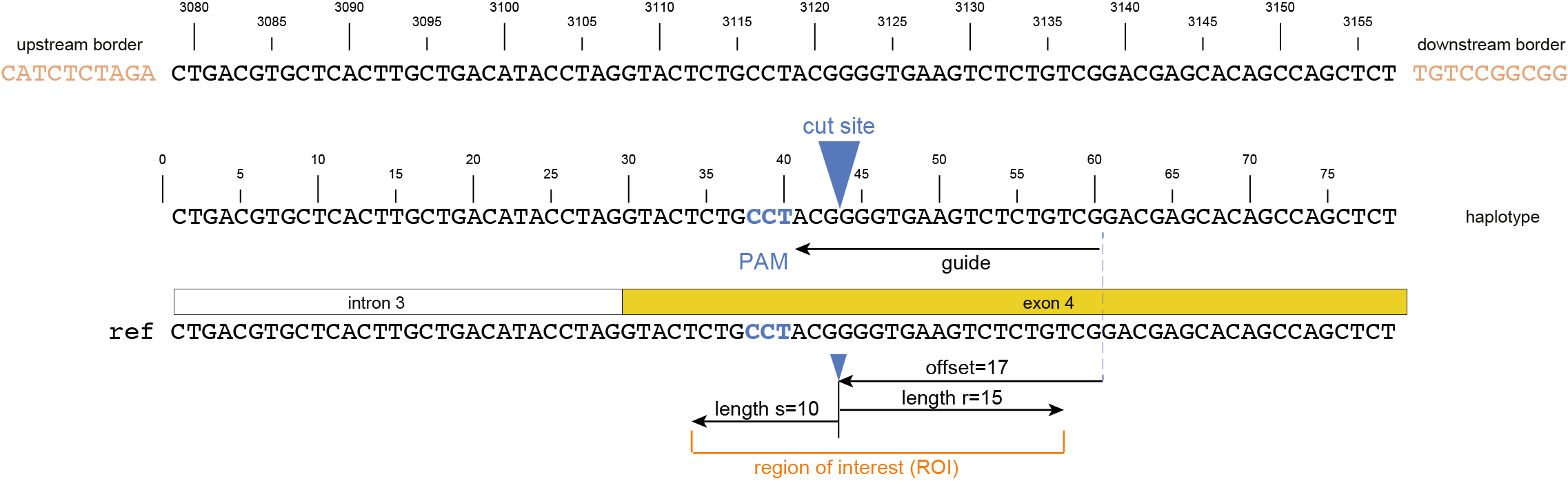
In case of CRISPR/Cas-induced mutations, a short region surrounding the gRNA binding site, adjacent to the PAM site where Cas acts on the DNA (either by cutting, base-editing, or other modifications) is considered. This region of interest (ROI) is defined by the PAM sequence (Cas-enzyme dependent), the distance between the PAM site and the expected cut-site (offset), the region upstream (in the direction of the PAM site) and downstream (away from the PAM site) from the expected cut-site in which mutations are expected. Any sequence variant that overlaps with the ROI by at least one nucleotide, is considered relevant for SMAP effect-prediction. All other sequence variants outside the ROI (such as neighboring SNPs, read errors, indels far away from the expected cut-site, or extra nucleotides near the borders resulting from poor trimming by SMAP haplotype-window) will be considered as reference sequence and ignored for estimating the resulting protein sequence.
Step 2. Align
Align each haplotype to its reference per locus


Each alternative haplotype is aligned to it’s reference haplotype sequence of the corresponding locus. The reference sequence is retrieved from the coordinates of the borders of that locus provided as GFF file, and the reference sequence FASTA file. Here, the alignments of locus gene3_1 of the example data set are shown. Insertions in the alternative haplotype are shown in green, SNPs are shown in red.
Step 3. Filter and collapse
Filter for haplotypes based on location of sequence variants within the window: region of interest (ROI)
SMAP haplotype-window extracts all observed unique DNA sequences within a user-defined window and calls these haplotypes. So, artefactual haplotypes may be created by sequence variation such as read errors, imprecise trimming, etc. SMAP haplotype-window allows to filter the genotype call table based on haplotype frequency, but not on sequence content. To further eliminate artefactual haplotypes and collapse the genotype table into a simpler matrix with less haplotype complexity, SMAP effect-prediction implements an optional filter that only retains sequence variants that overlap with a given ROI.
3.1. Definition of the ROI.
Because there is no prior focus or knowledge on where naturally occurring sequence variants may be located, the ROI typically spans the entire length of the locus.
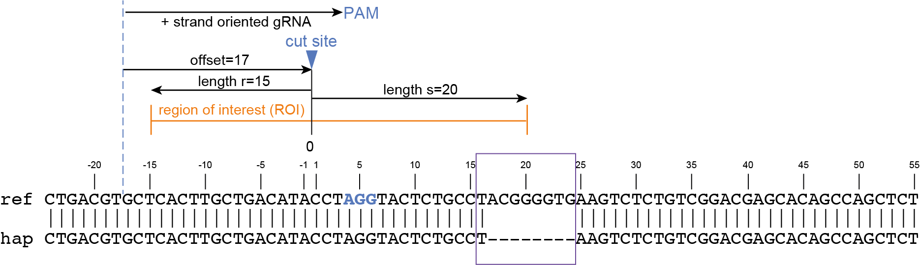
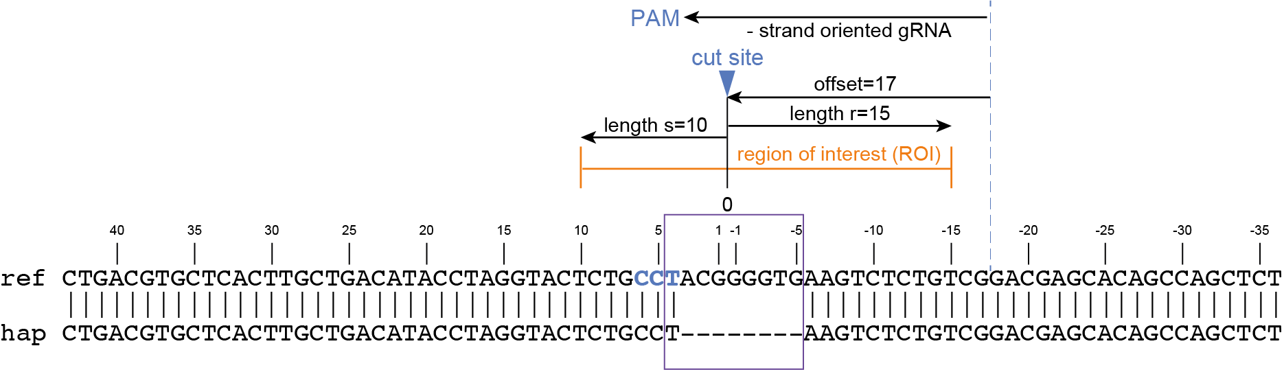
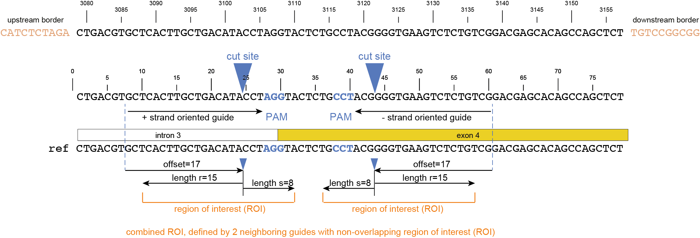
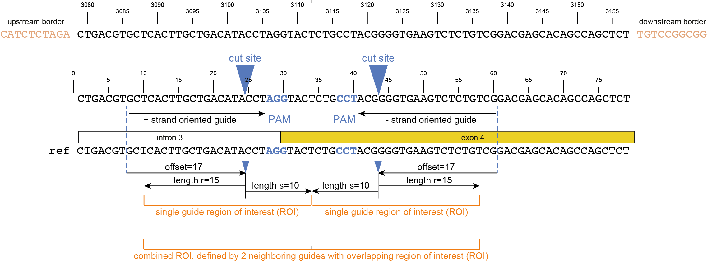
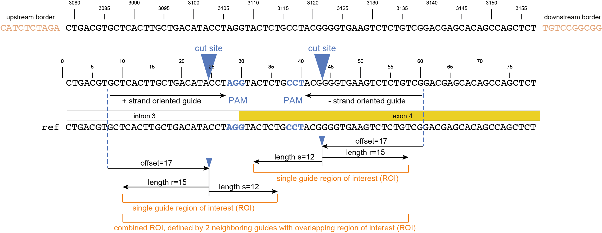
3.2. Filtering on the ROI.
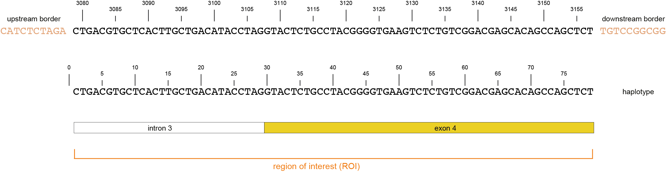
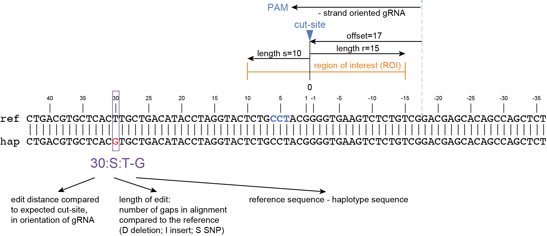
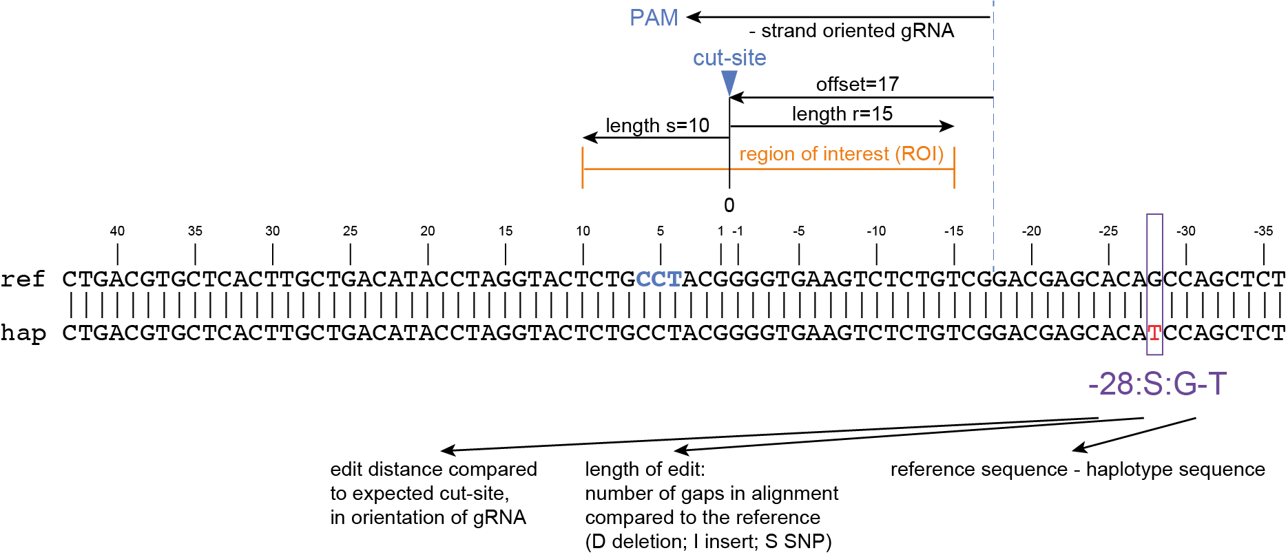
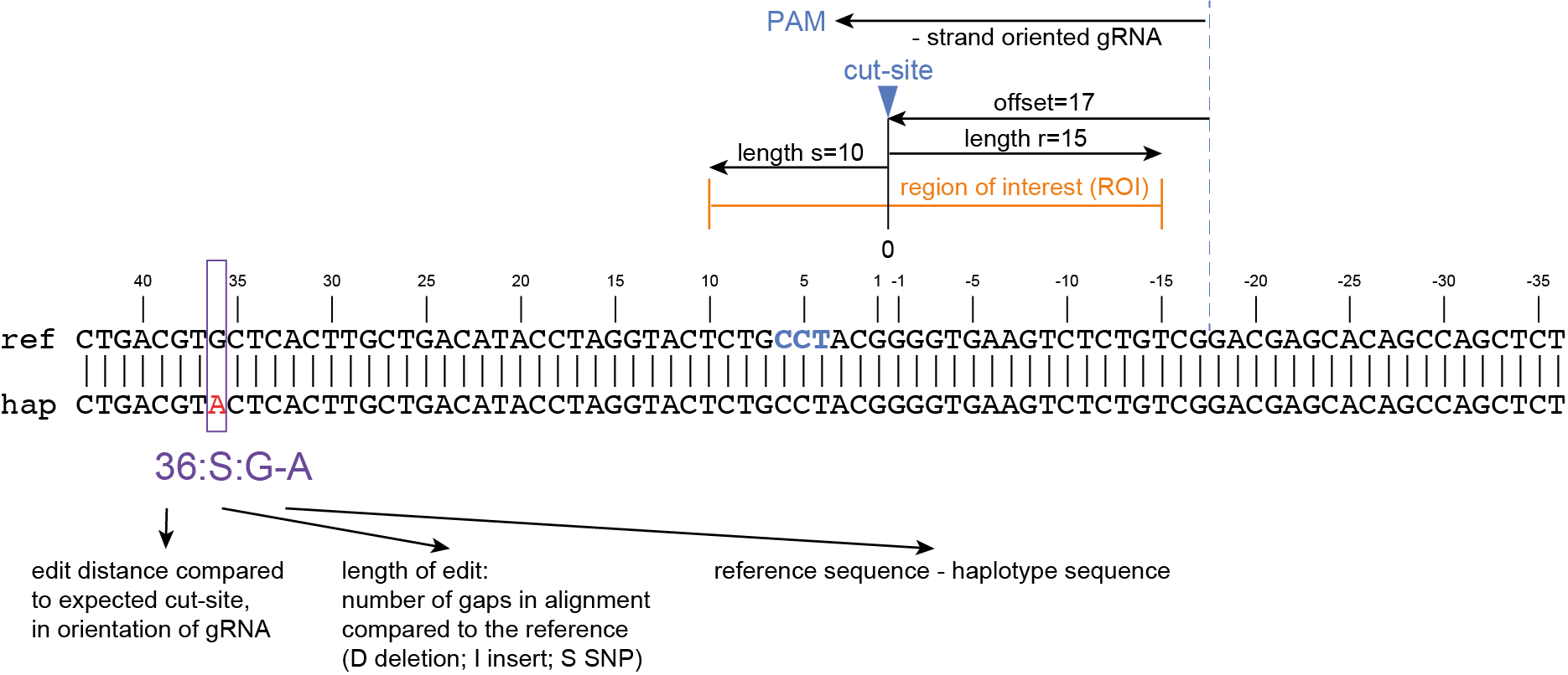
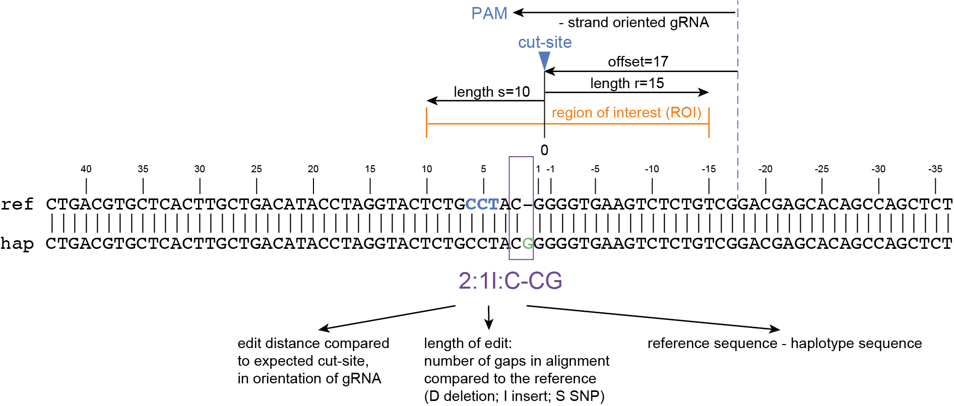


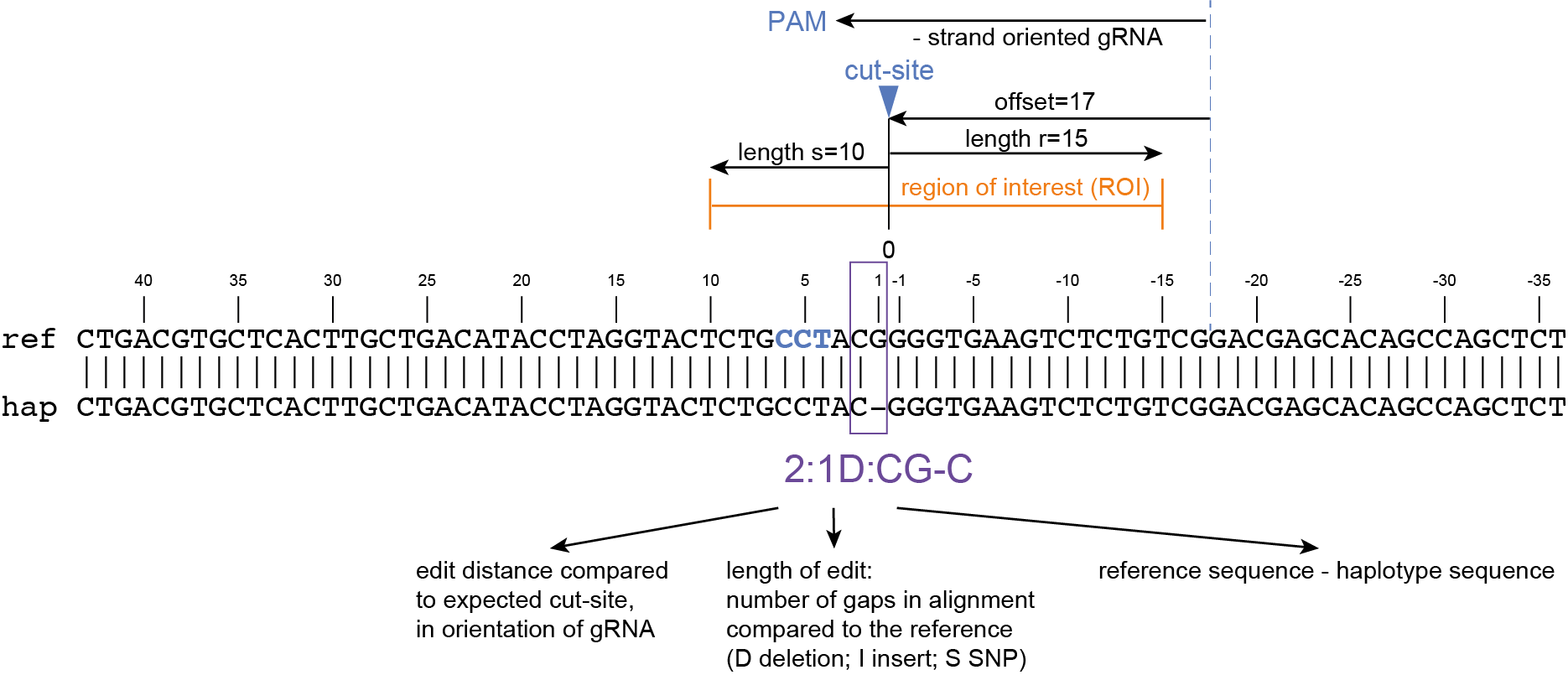
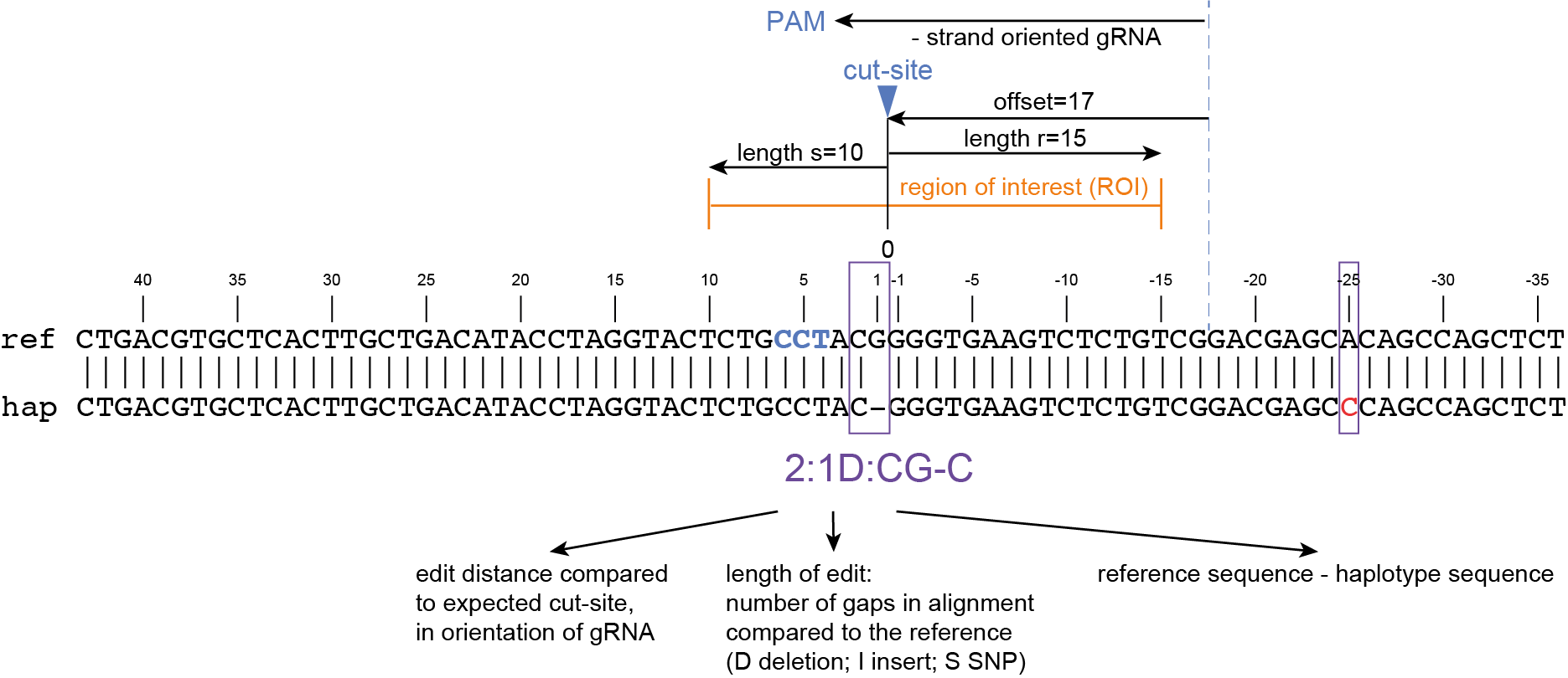
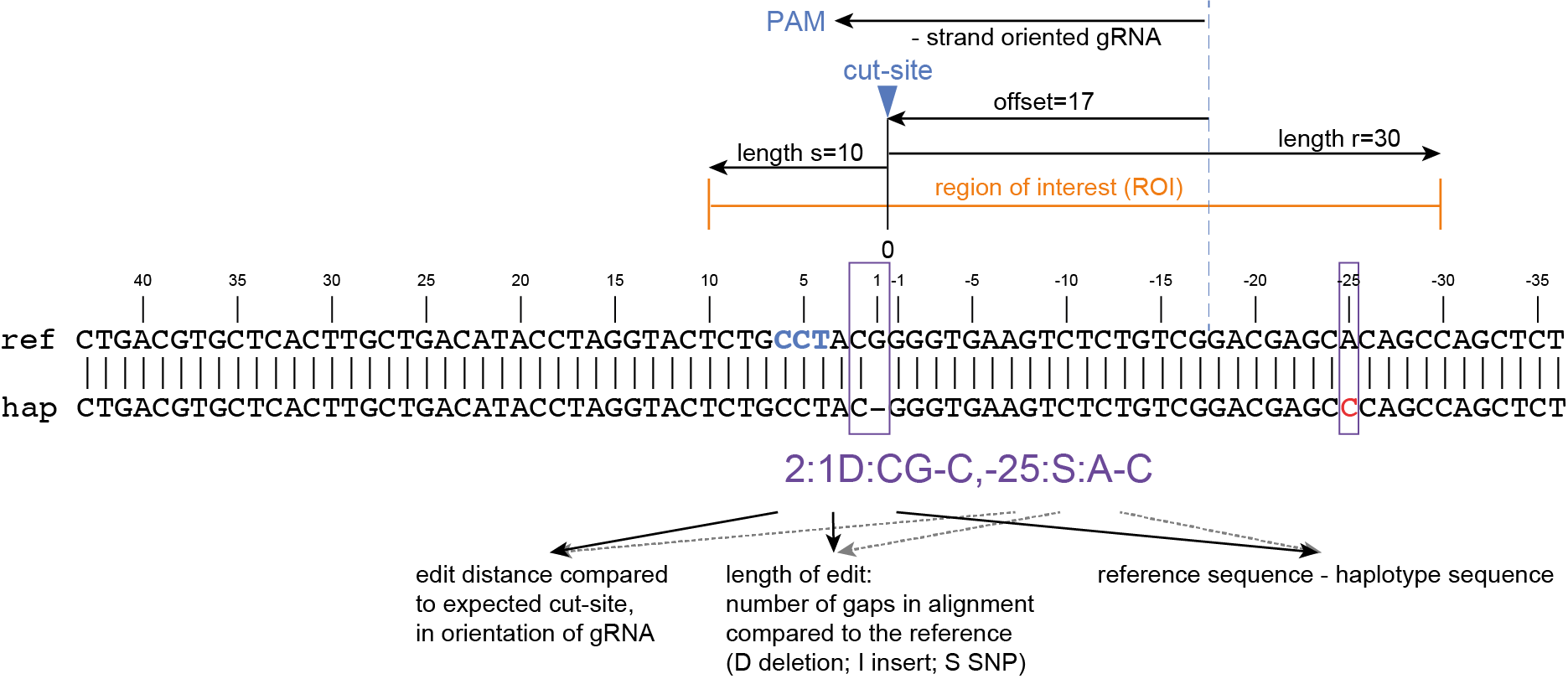

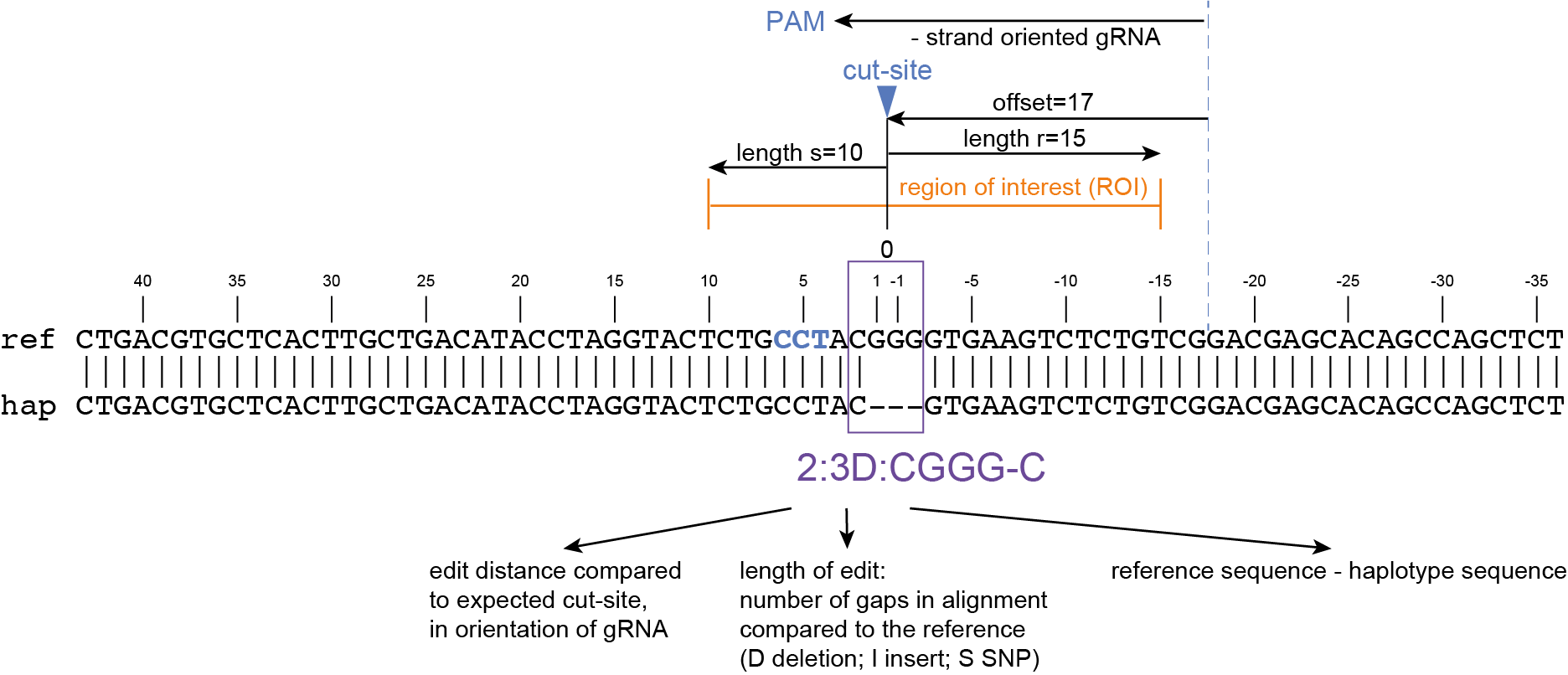
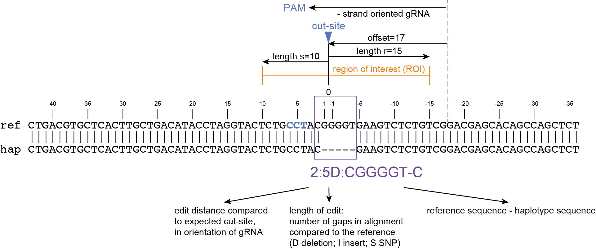
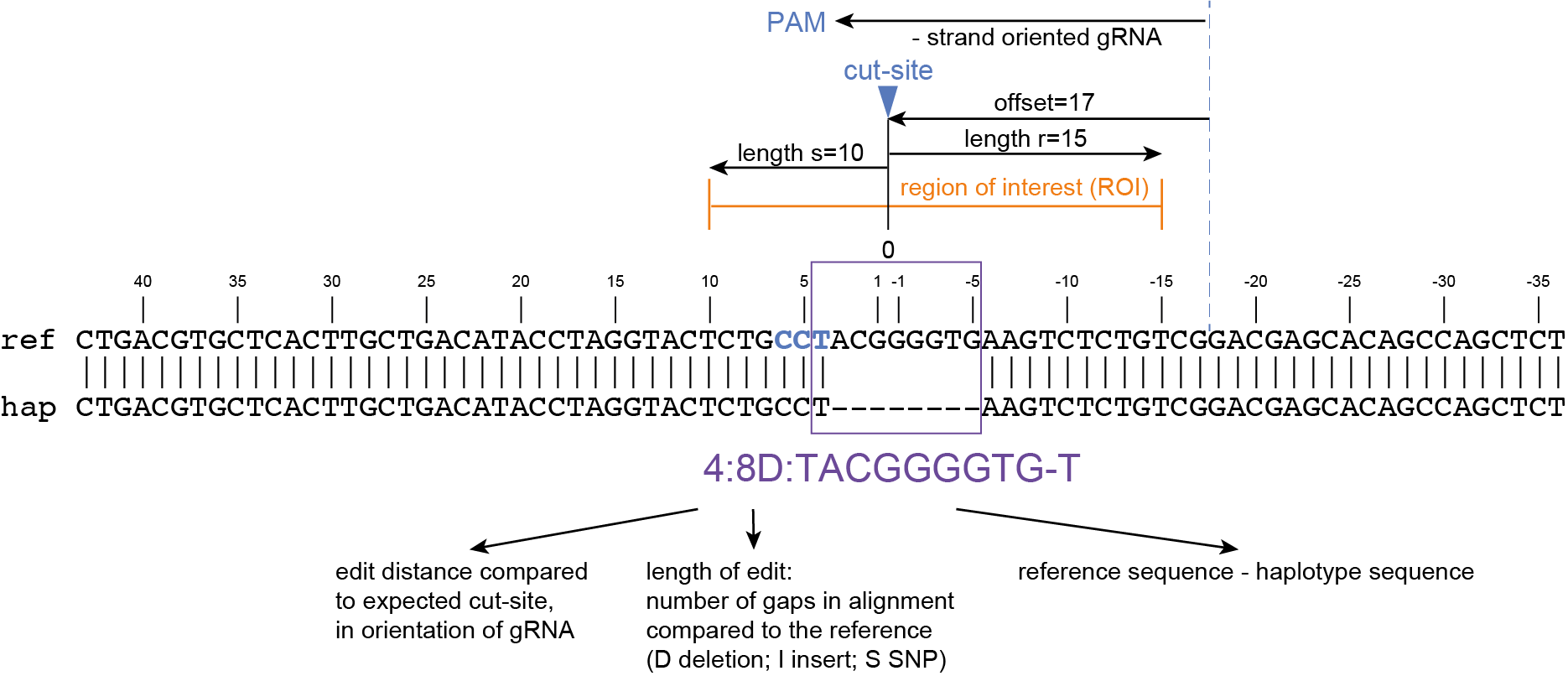
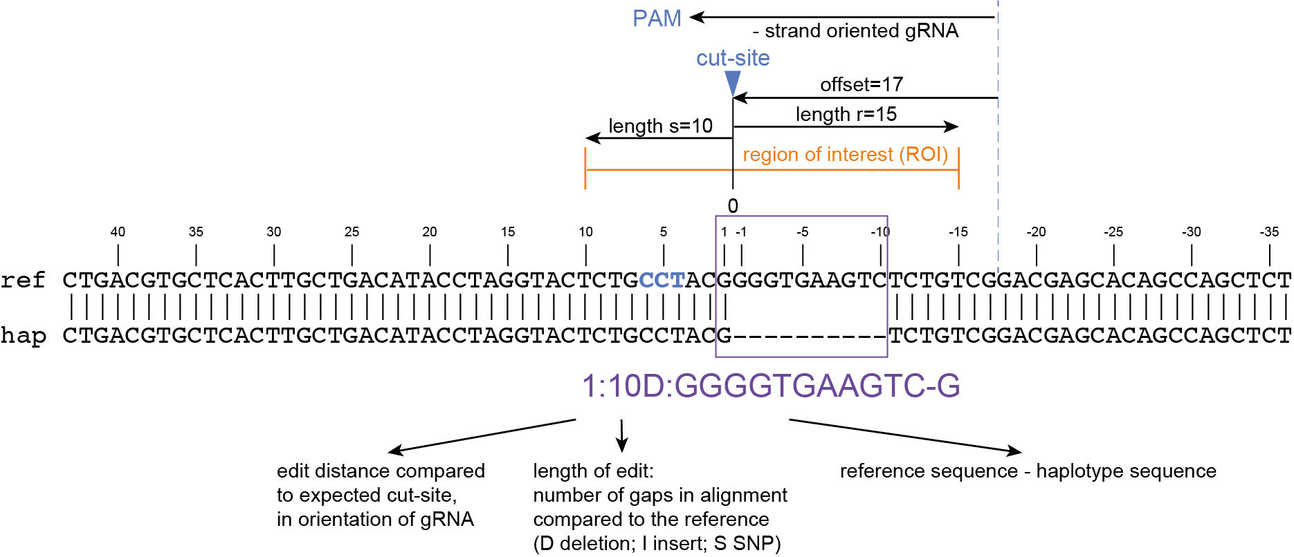
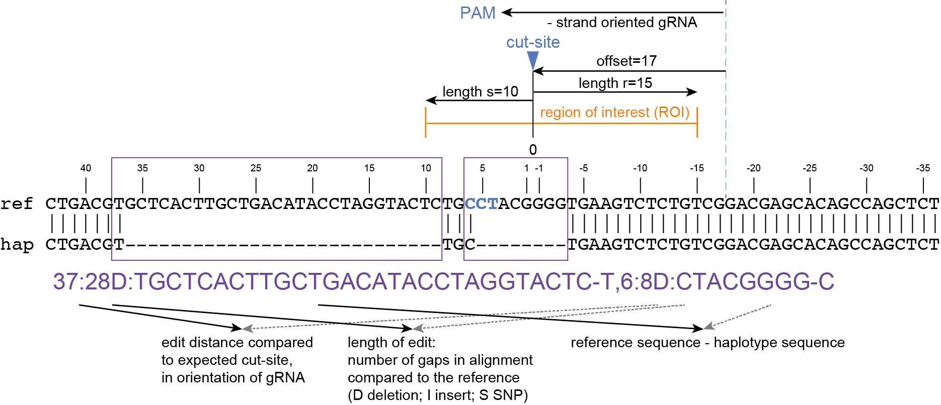
3.3. Collapse the haplotype table based on identical haplotype calls in the region of interest (ROI).
After exclusion of sequence variants outside the ROI, some haplotypes may contain identical haplotype calls within the ROI.
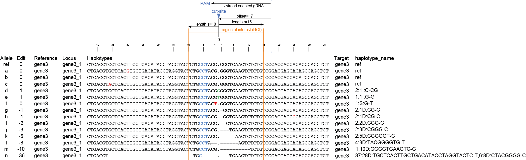
If the user decides to ignore sequence variation outside the ROI, the algorithm ‘collapses’ corresponding haplotypes by summing their relative frequencies in the haplotype table. Accordingly, the haplotype frequency table switches to new haplotype identifiers per locus, because the exact DNA sequence that initially identified the unique haplotypes no longer correspond to the ‘collapsed’ sequences.
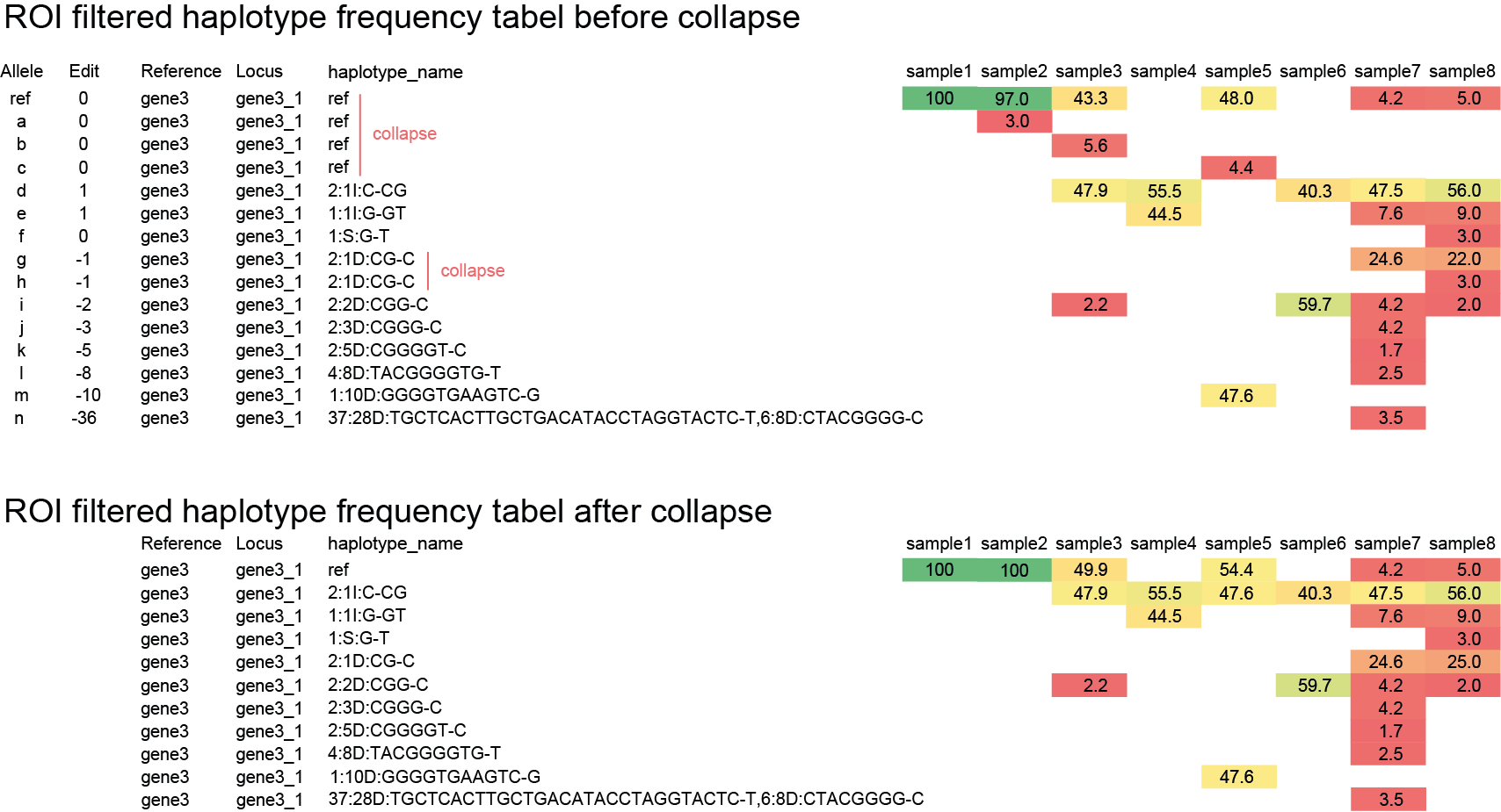
Step 4. Annotate
Annotate the haplotype, score effects on gene structure and predicted protein sequence.
SMAP effect-prediction uses the local GFF file provided by the user to extract gene structure annotation and place the haplotype back into its genomic context. For each haplotype, the corresponding full length mutated protein sequence is reconstructed and mutations in strategic sites (START codon, splicing sites, and STOP codon) are searched. At the end of the process, the master table is extended with more columns further describing the computationally predicted effect of each haplotype on the protein. The steps to annotate the master table are as follows:
4.1. Delineate the CDS region in the window by creating a reference ‘CDS code’.
Using the local GFF file provided by the user, SMAP effect-prediction identifies the genomic areas corresponding to coding sequences (CDS). The CDS regions are encoded as 1 and the non-coding areas as 0. The reference genome sequence is thereby simplified into a string of 0’s and 1’s, here named the “CDS code”. The file with border positions is used to identify the position of the haplotype both in the genome sequence and in the CDS code. The reference and mutated haplotype are extracted from the master table and the haplotype CDS code is extracted from the CDS code using the border positions. Regions outside the borders in the genomic and CDS code sequences are kept for later stages.
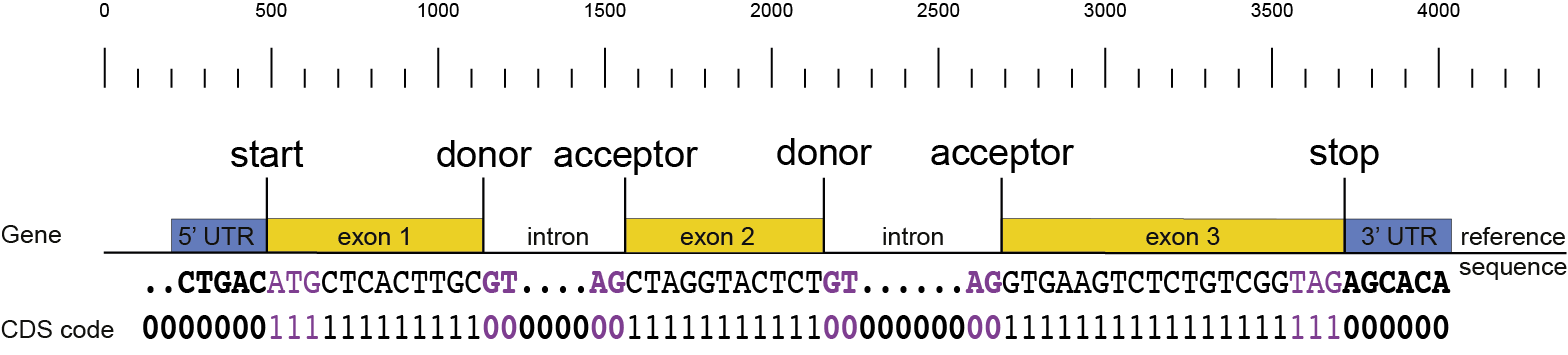
4.2. Identify indels and modify the ‘CDS code’.
The alignment between the reference and mutated haplotypes (see Step 2 Align) is used to identify indels. The alignment is screened for gaps; insertions are represented by gaps in the aligned reference haplotype whereas deletions are shown by gaps in the aligned mutated haplotype. Indel indices are captured, and the reference haplotype CDS code is modified accordingly, so that its indexing now matches the length of the alignment and fits the mutated haplotype CDS sequence.
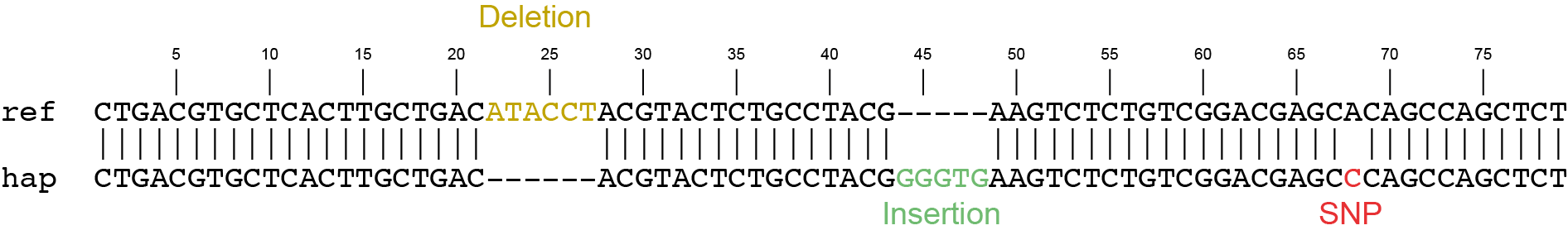
Insertions and deletions in the haplotype CDS code are treated differently.
Insertions
For instance, if a +5 bp insertion is observed between positions 43 and 44 in the reference sequence, the haplotype CDS code will be extended by 5 characters at the same index. The mutated haplotype has a longer length compared to the reference haplotype, and so the mutated haplotype CDS code must be extended too. The rules to know which character (either 0 or 1) has to be used for extending the haplotype CDS code are as follows:
If positions surrounding the insertion are coding in the haplotype CDS code (i.e. 1), then the insertion is considered as coding (i.e. made of extra 1’s).
If positions surrounding the insertion are non-coding in the haplotype CDS code (i.e. 0), then the insertion is considered as non-coding as well (i.e. made of extra 0’s)
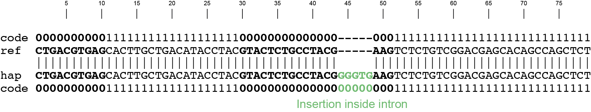
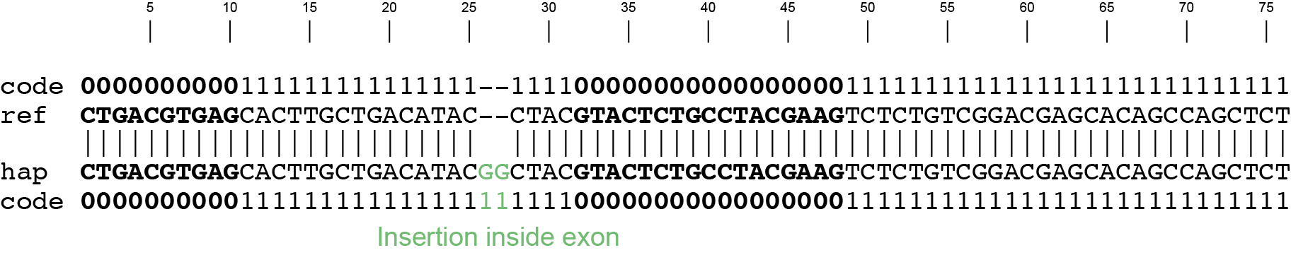
If one of the positions surrounding the insertion is coding (1), and the other is non-coding (0), this means that the mutation occurs right after or right before a splicing site. In both cases, the insertion is considered as coding.

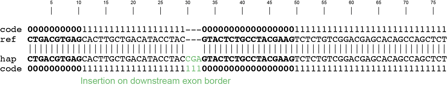
Deletions
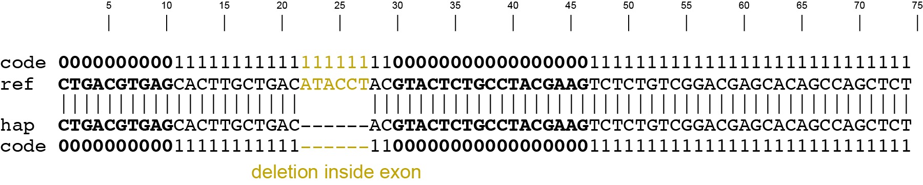
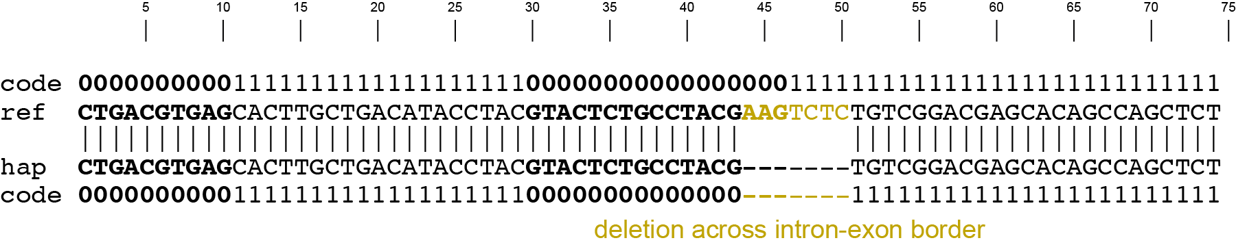
In the case of a deletion, the indices of the deletion in the reference haplotype are simply removed from the haplotype CDS code. The mutated haplotype has a shorter length compared to the reference haplotype, and so does the mutated haplotype CDS code.
SNPs
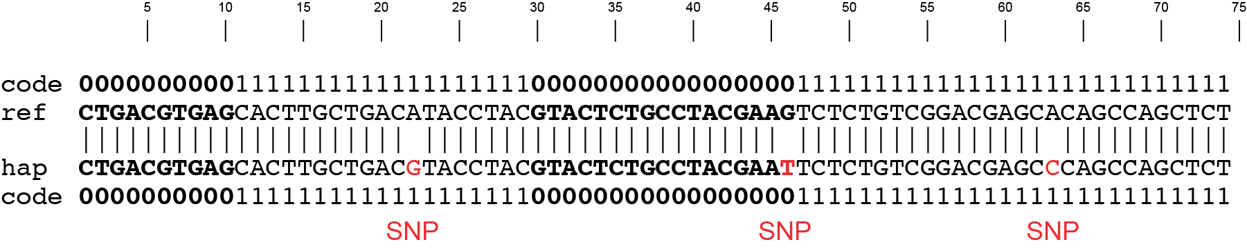
In case of SNPs, no gaps are observed in the alignment (only mismatches). The indexing is the same between the non-aligned and aligned reference and mutated sequences so the haplotype CDS code is not modified. SNPs in coding areas are assumed to be coding and SNPs in non-coding areas are assumed to be non-coding.
4.3. Place CDS codes of reference and mutated haplotypes back into their genome context.
The mutated haplotype sequence and the mutated CDS code are placed back into their respective context. Both sequences are stitched back with the reference regions outside the borders that were kept at step 1 of the annotation process. This results in a full genome sequence with mutation in the haplotype area and a full CDS code of the same length with altered sequence in the haplotype area.
4.4. Search for mutations at translational START and STOP codons and splicing sites.
Before translating the mutated genomic sequence using the mutated CDS code, strategic sites are searched for mutations. SMAP effect-prediction will consider that any modifications at the translational START codon is a major effect. Because SMAP effect-prediction can not reliably predict translation re-initiation that might occur at a downstream alternative translational START codon, it is not possible to compute an alternative protein sequence. The resulting identity score between the reference and the mutated protein is by definition 0. Likewise, modifications at splicing sites are considered major effects. Because SMAP effect-prediction cannot reliably predict which downstream splicing donor or acceptor site will be used, the algorithm simply truncates protein translation right at the position of the mutated splicing donor or acceptor site. Finally, mutations at the translational STOP codon lead to an extended open reading frame (ORF) at the 3’ end, and the translation continues until it reaches the following STOP codon in the ORF.
4.5. Extract and stitch all CDS sequences to create a full length CDS.
The mutated protein is obtained using the mutated genomic sequence and the mutated CDS code. Coding areas are extracted and stitched together to form the full CDS. The mutated CDS is then translated, considering possible mutations at strategic sites (see step 4 of the annotation process).
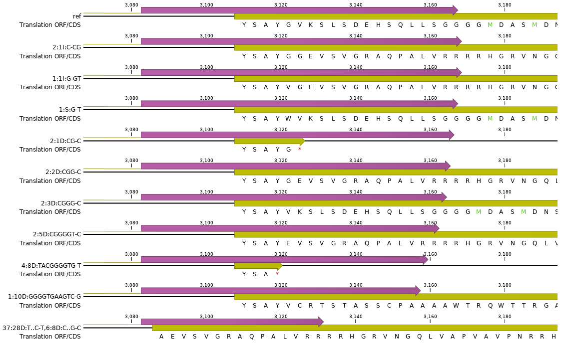
In-silico translation of the haplotypes of gene3. Amplicons (gene3_1) were projected into their respective gene context and translated in the corresponding ORF.
4.6. Align reference and mutated protein and calculate %identity score.
The reference and mutated protein are aligned. The number of identical amino acids in the alignment is computed and divided by the total length of the alignment and expressed as percentage to obtain the identity score (see also Grant lab, Girgis et al., 2021, EBI).
ref ML--IIFGLA
    ||  ||| ||
mut MLDKIIF-LA
In case the original protein is much longer than the mutated protein, the two proteins are aligned globally so the length of the alignment is 16, but only 7 amino acids are identical in the alignment.
ref ML--IIFGLATLGHWS*
    ||  ||| ||
mut MLDKIIF-LA*
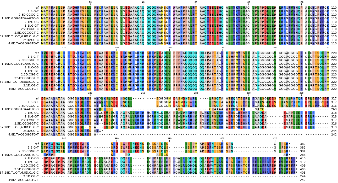
Alignment of the predicted proteins encoded by haplotypes of gene3.
4.7. Add the novel annotation columns to the haplotype frequency table.
The master table is annotated and extended with five more columns:
atgCheck: whether the ROI in the haplotype contains a mutation affecting the START codon: True/False
splicingSiteCheck: whether the ROI in the haplotype contains a mutation affecting a splicing site: True/False
stopCodonCheck: whether the ROI in the haplotype contains a mutation affecting the STOP codon: True/False
protein_sequence: the full length mutated protein sequence
pairwiseProteinIdentity: the %identity score between the reference and mutated proteins as explained at 6.
Step 5. Classify loss-of-function effect of mutation on protein per haplotype: LOF effect classes
quantify the effect on gene function or activity based on the %identity score
The user can define the %identity cutoff to declare that a mutation has an effect on the protein function or activity, based on the protein identity score computed in the previous step (see step 4.6. of the annotation process). The degree of loss-of-function (LOF) can be discretized in three discrete effect classes: no or minimal effect, intermediate effect, strong effect (knockout, KO). Haplotypes leading to substantial loss of the protein sequence are expected to cause major protein disruptions and are therefore considered as loss-of-function (LOF) or knockout (KO) haplotypes. For instance, at a cutoff of 70%, haplotypes with %identity score below 70 are considered major effect mutations, whereas haplotypes with %identity score greater than 70%, are considered to not have a major effect on the protein (i.e considered as functional as reference).
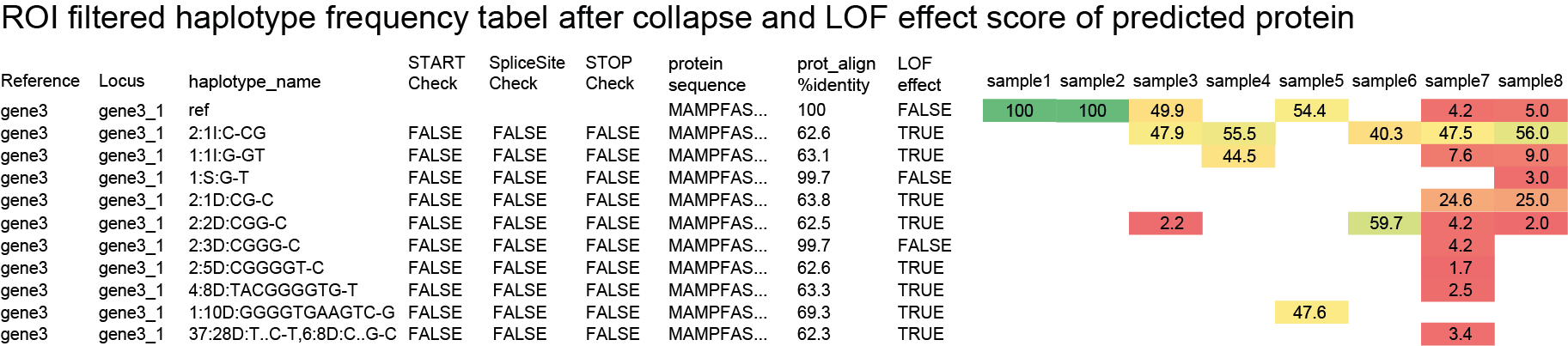
Step 6. Aggregate haplotype frequencies per locus by LOF effect class
Aggregate the frequency values of haplotypes that have at least a minimal degree of LOF: per locus, per sample
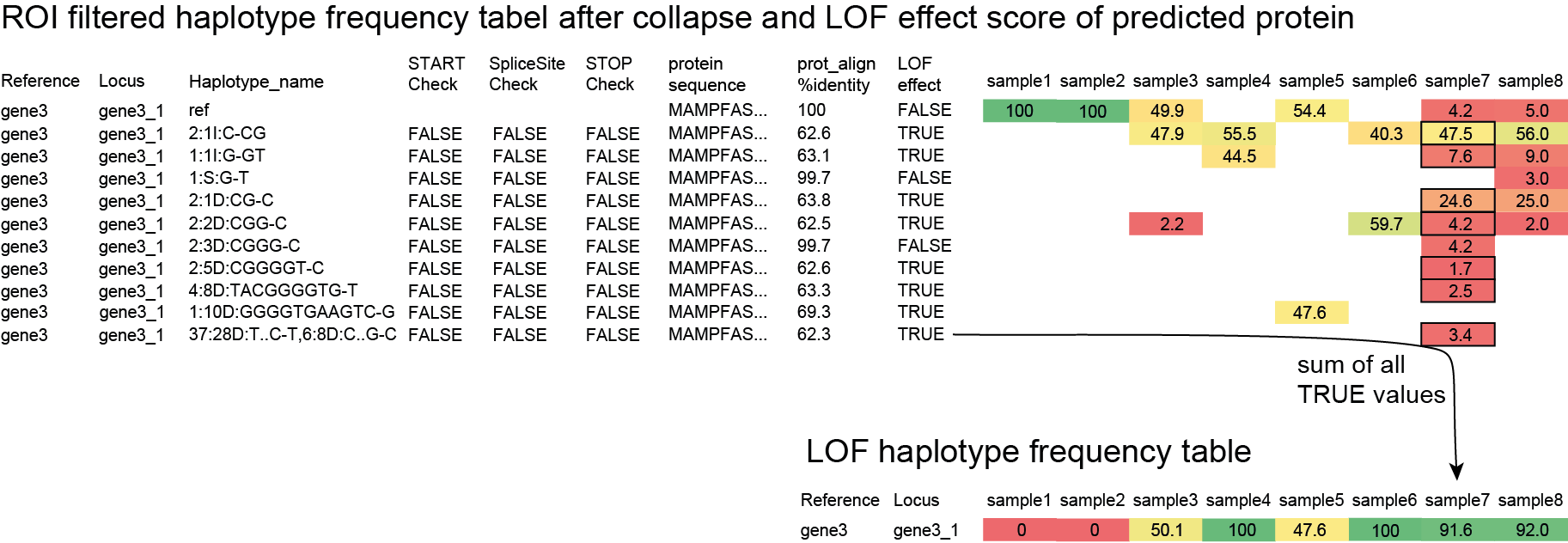
The frequencies of LOF haplotypes are summed per locus per sample to display the relative fraction of proteins with at least a minimal degree of LOF. The resulting aggregated genotype call table contains the cumulative frequency of all haplotypes encoding a LOF protein (one value per locus per sample on a scale of 0-1; where 0 indicates all reference protein, and 1 indicates all LOF protein).
Step 7. Discretize
Transform cumulative LOF frequency to discrete genotype calls: WT, heterozygous KO, homozygous KO
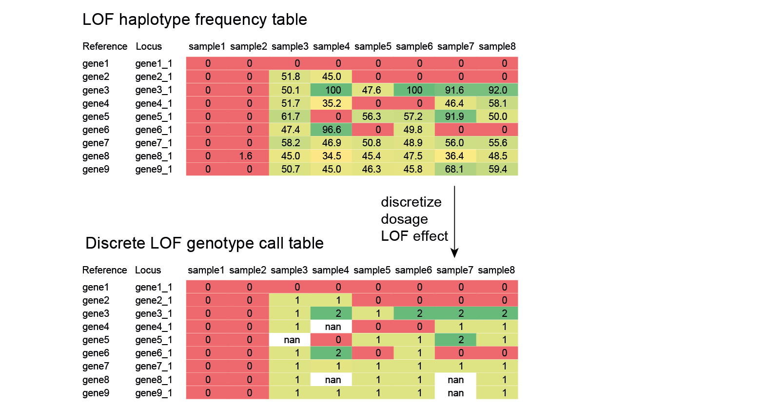
Aggregation of KO haplotype frequencies leads to a quantitative LOF frequency distribution that is difficult to interpret in genetic analysis. The aggregated KO haplotype frequency has a W-shape distributions in diploid samples. Local maxima are located around values of aggregated KO haplotype frequency of 0, 50%, and 100% which corresponds to homozygous reference, heterozygous KO, and homozygous KO, respectively. Indeed situations where half of the reads are KO haplotypes and half are not highlight heterozygosity in a diploid organism. SMAP effect-prediction can transform the quantitative KO haplotype frequency into discrete genotype calls, homozygous reference, heterozygous, homozygous mutant, coded as 0, 1, and 2, respectively. The frequency intervals to call such genotypes can be user-defined. As a rule of thumb, we generally consider that <15% is homozygous reference, between 40% and 60% is heterozygous, and >90% is homozygous mutant. These cutoffs can be adjusted after inspection of the graphical output after a first analysis. The discretization further eases the interpretation of the table, especially in the case of Mendelian segregation in progeny, or downstream statistical analyses to associate phenotypes to genotypes. Discretization may also be performed before aggregation of haplotypes per locus so that one can associate phenotype per haplotype rather than per locus.