Feature Description

The module SMAP effect-prediction is designed to help interpretation of the sequence variants in haplotype call tables created by SMAP haplotype-window.

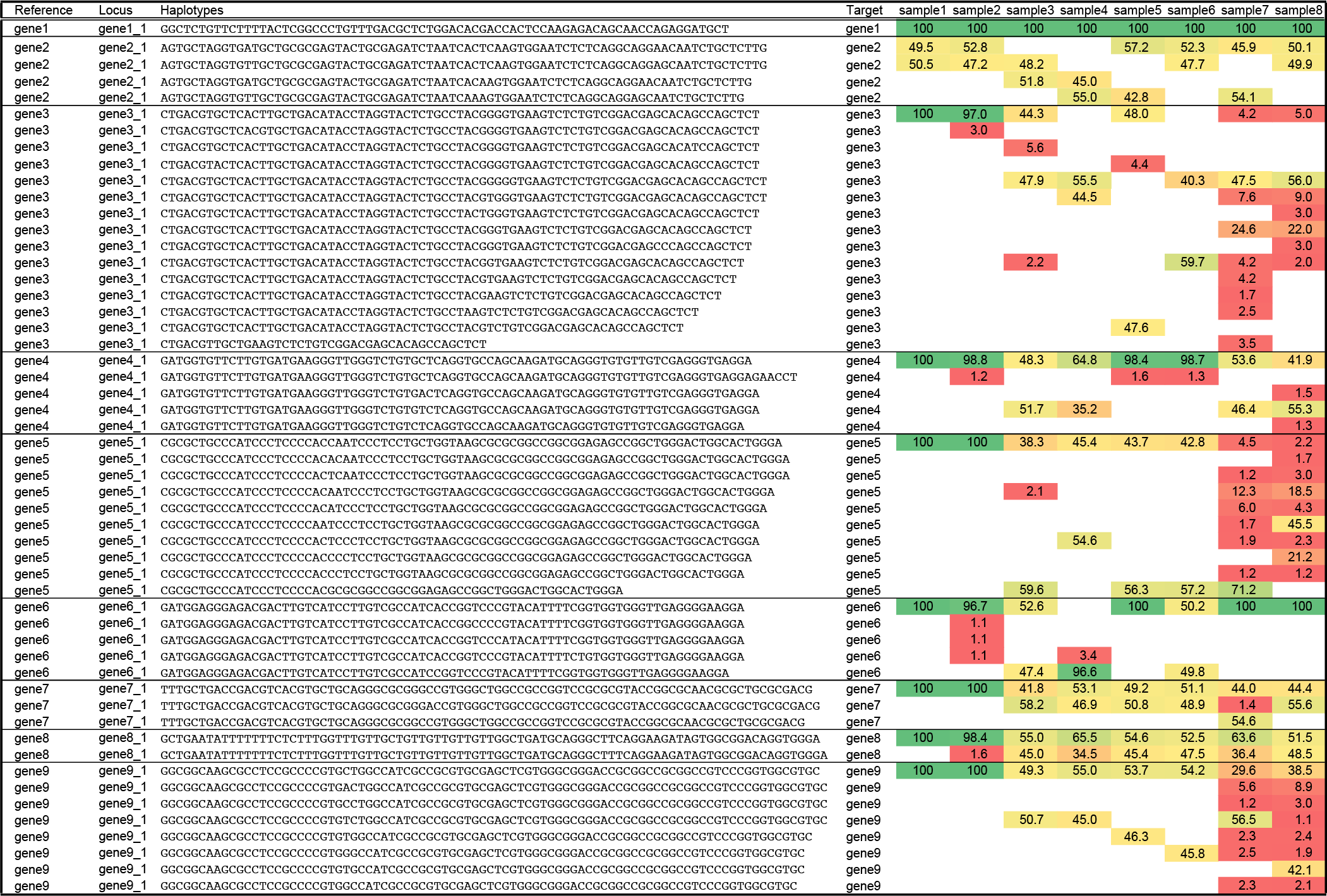
Below, we first illustrate the various biological causes of haplotype sequence variation and typical haplotype frequency distributions, and then explain the underlying concepts driving the subsequent steps of SMAP effect-prediction. A typical example of a SMAP haplotype-window genotype call table on nine loci scored in eight samples is presented below. For each locus, the observed haplotypes are listed, and per sample the relative frequency of each haplotype is quantified based on the total read depth per sample per locus. Loci are defined by two border sequences on the reference genome that flank a window of interest, and each haplotype is the exact, unique DNA sequence within that window. See the manual of SMAP haplotype-window for further details.

Interpretation of the induced mutation spectrum in a plant collection

The output of SMAP haplotype-window is a tab delimited text file. For ease of reference, the first two columns (alleles, Edit) have been added here to indicate the kind of information that can be derived from the genotype table. Alleles are named in the column Allele (“ref” for reference haplotype; and a-n for unique alternative haplotypes), their length difference compared to the reference is indicated in the column Edit. Haplotypes are grouped per reference sequence (gene1-gene9), and per locus (gene1_1-gene9_1), one amplicon per gene, indicated by horizontal boxes. The exact, unique haplotype is defined by the DNA sequence extracted from the sequencing read data (typically HiPlex sequencing), delineated by two borders. Next, the relative haplotype frequency is indicated in false colour (green, high frequency - homozygous; yellow, intermediate frequency - heterozygous; red, low frequency - noise). In the schemes further below, the haplotypes are aligned to the reference and annotated for easier interpretation of the sequence polymorphisms. A “.” indicates a gap in the alignment adjusting for a +1 bp insertion in one of the alternative alleles, a “-” in the alignment indicates a gap due to deletions in the alternative alleles. SNPs are indicated in red, inserted nucleotides are indicated in green, PAM (NGG) sites are indicated in blue.

Wild type samples and reference haplotypes, locus gene1_1.

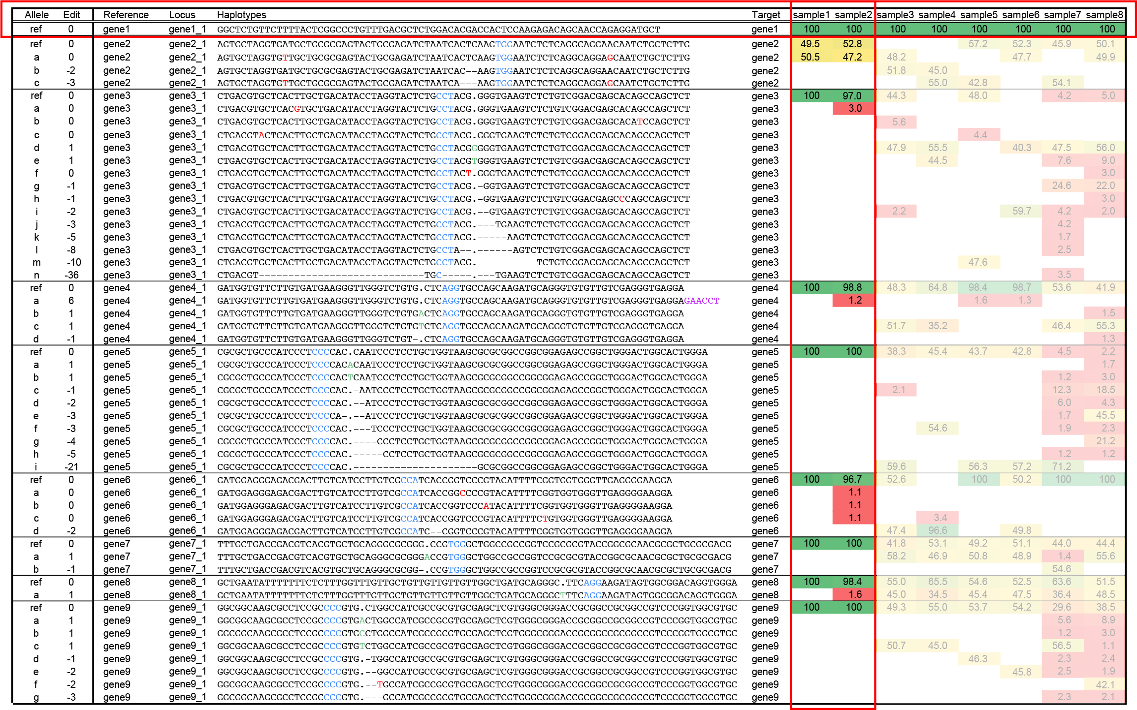
Sample1 represents a wild type sample, in which only reference haplotypes are detected (at 100% of the read depth in all loci except gene2_1; see explanation on heterozygous loci below), and no other haplotypes. Sample2 also represents a wild type sample in which the reference haplotypes are detected for all loci, and in addition a few other haplotypes at very low frequency. Such haplotypes are considered noise and may be eliminated by SMAP haplotype-window using option -f to filter out haplotypes with low frequency across all samples, or option -m to mask low frequency haplotypes on the per-sample level. For locus gene1_1, only reference haplotypes are detected and there are no signs of genome editing in any of the plants in the collection (sample3-sample8).

Simple cases of homozygous and heterozygous genome editing, loci gene6_1, gene7_1, gene8_1.

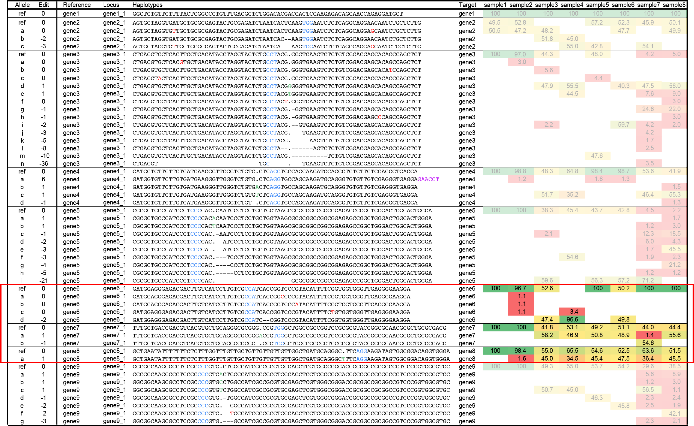
Simple cases of genome edits display two characteristic features: mutations are located close to the PAM site in the target sequence, and two distinct haplotypes with relative frequency around 50% correspond to heterozygous state edits in a diploid organism (of which one may be the reference haplotype). A homozygous locus is defined as a single dominant haplotype at >90% of the read depth per locus (allowing for some low frequency spurious haplotypes).

Ambiguous cases of haplotype diversity: SNPs outside ‘expected’ edit region (false positives), locus gene6_1.

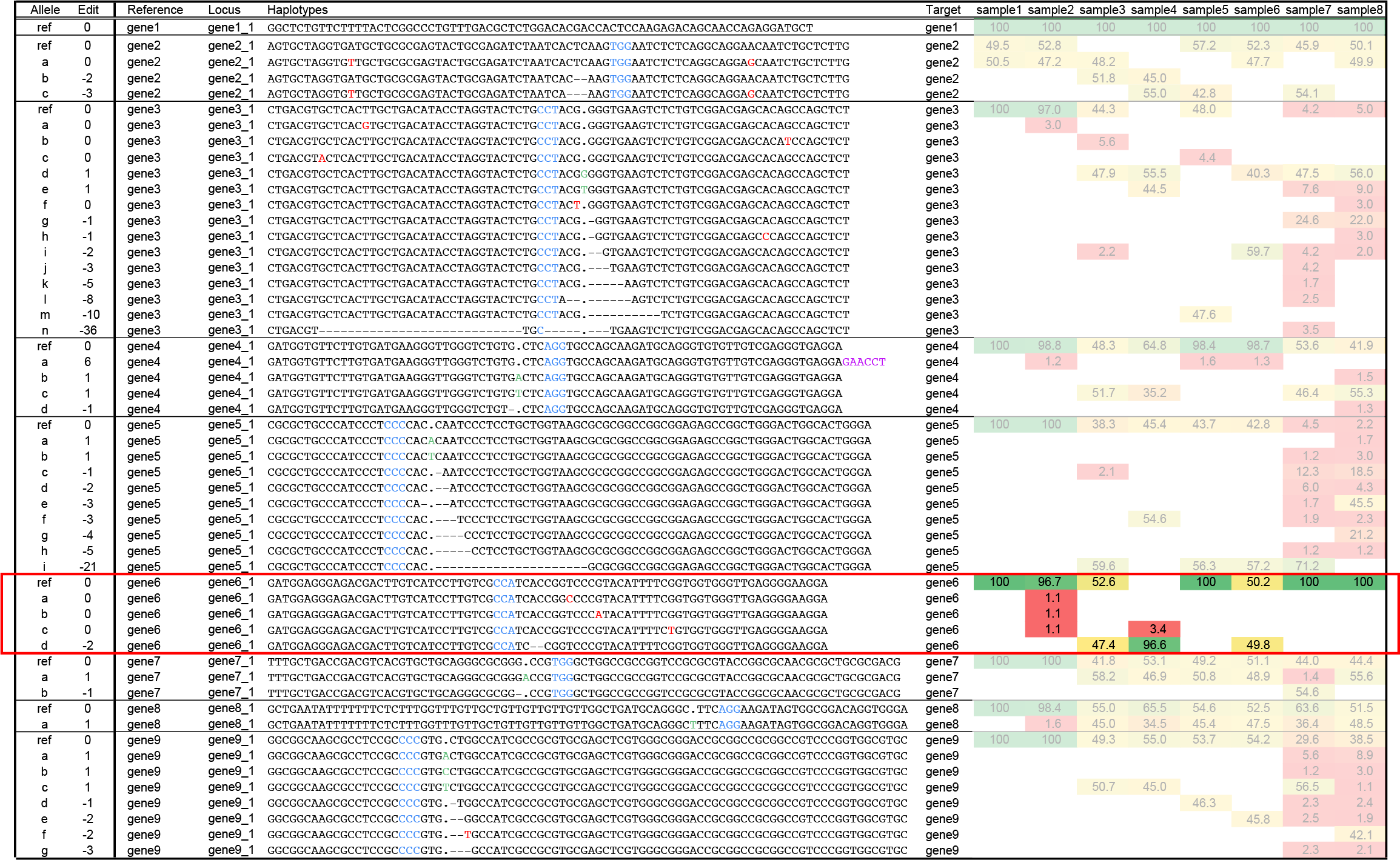
Locus gene6_1 displays haplotypes with equal length but a different sequence compared to the reference. These unique haplotype sequences may be caused by SNPs (indicated in red) located near, or outside of the ROI, and may be the result of amplification or sequencing artefacts rather than true haplotypes. Such haplotypes can either be removed by a low frequency filter or mask in SMAP haplotype-window, or alternatively, by setting the ROI in SMAP effect-prediction.

Ambiguous cases of haplotype diversity: wild type samples with heterozygous loci of two haplotypes, locus gene2_1.

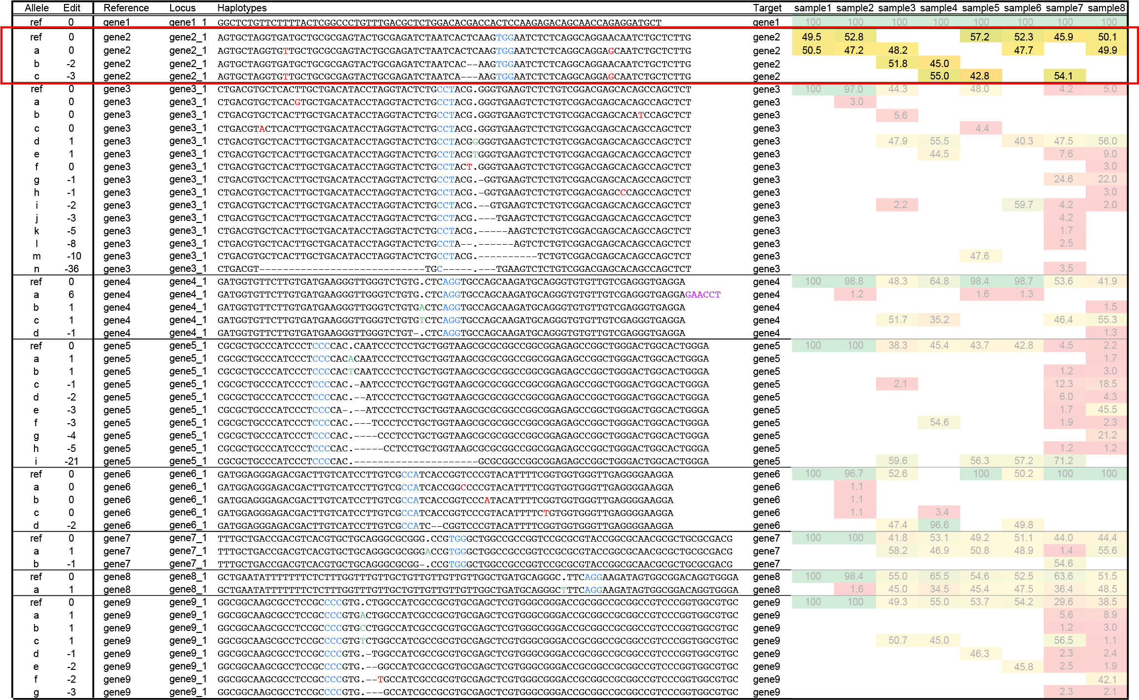
Locus gene2_1 displays two haplotypes with equal length but a different sequence compared to the reference in both wild type sample1 and sample2. This indicates that the genotype used for genome editing has a heterozygous background. The two SNPs that differentiate the haplotypes (indicated as red nucleotides in haplotype a), are far away from the gRNA binding site and both alleles can be targetted for genome editing in the central region of the haplotype. As a result, two distinct edited alleles occur, one that shares the sequence flanking the -2 bp gene edit with the reference, and the other haplotype shares the sequence flanking the -3 bp gene edit with the second allele. Because the reference genome typically contains only one representative sequence per locus, only the haplotype with an exact match to the reference genome is named “ref”. This example shows that allele specific editing can be identified using SMAP haplotype-window.

Many different haplotypes may be detected per locus across samples, loci gene3_1, gene5_1, gene9_1.

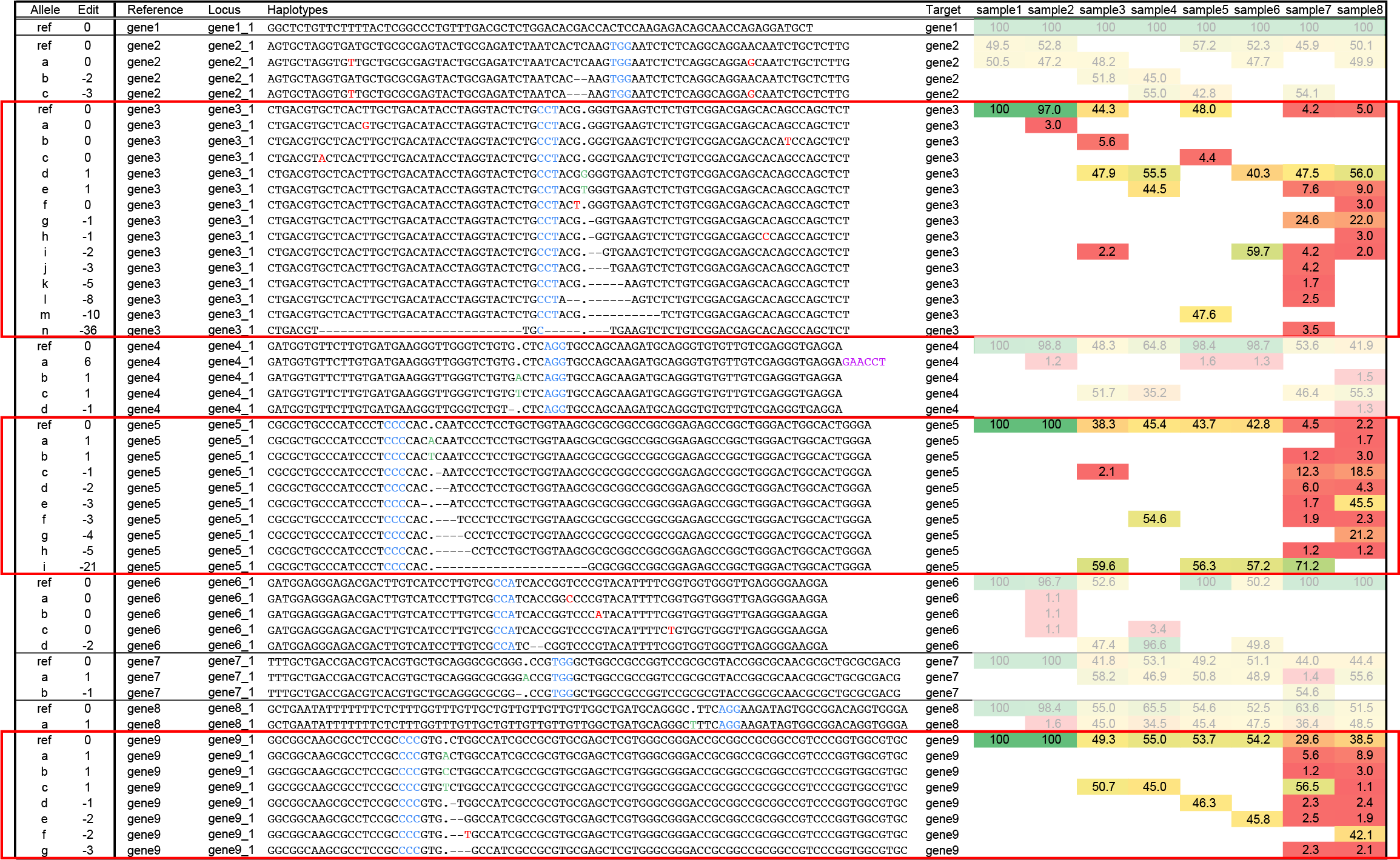
Because double stranded breaks depend on error-prone non-homologous end joining (NHEJ) repair mechanisms, and every plant creates independent mutations, there may be a range of different editing outcomes per locus across the collection of plants. For instance, locus gene9_1 shows at least 7 novel haplotypes (haplotypes a-g) across the different samples. All haplotypes show mutations around the expected cut-site (near the PAM). Haplotypes c,d,e,f are observed at relatively high frequency (around 50%, likely heterozygous state) in sample3, sample4, sample5, and sample6. Haplotypes a and b are detected only at low frequency in sample7 and sample8, but their haplotype corresponds to a single nucleotide insertion (coloured green) at the expected cut-site, near the PAM, and haplotype g corresponds to a -3 bp deletion near the expected cut-site.

Many different haplotypes may be detected per locus within a sample: signs of active editing and mozaicism, loci gene3_1, gene5_1, gene9_1.

Active editing within plants may generate more unique haplotypes than expected based on the ploidy of the plants. If a stable transgenic plant constitutively expresses Cas/gRNA complexes, this may lead to ongoing genome editing as long as the plant still contains cells with at least one reference haplotype as target of the gRNA sequence. Ongoing gene editing occurs independently in those individual cells, and can lead to variation in the editing outcome. In this way, a mozaic plant may be created that contains sectorial regions of cells sharing the same edit, while other parts of the plant may contain different edits derived from independent editing events. If such mozaic tissues are used for pooled DNA extraction, the diversity of edits may be detected in a single plant sample, for instance in loci gene3_1, gene5_1 and gene9_1, in sample7 and sample8. Mozaicism complicates genotype-phenotype associations as multiple haplotypes (which may each affect protein function in their own way) are present in different sectors of plant tissues, while plant phenotypes are often observed at the whole plant level (such as yield, leaf length, timing of flowering, or response to drought). Statistical analysis that determine genotype-phenotype associations thus have to deal with mixed signals in the genotype table within a single plant, or mixed signals have to be filtered, annotated, and/or aggregated to yield a single, unambiguous and discrete genotype call.

de novo haplotypes at subsequent generations.

Segregating populations may be created to obtain replicate plants of the constituent genotypic classes and/or to use mendelian segregation to separate the confounding effects of “stacked” mutations in multiple genes in a plant with a strong phenotype. If a backcross or selfing creates heterozygous mutated plants because the edited haplotypes are not both passed on through the gametes to the next generation, there are still reference haplotypes present in the progeny plant’s nuclei. In case genome editing is driven by stable transgenic plants constitutively expressing Cas/gRNA complexes, this may lead to de novo genome editing as long as the target of the gRNA sequence is not mutated yet. This means that apart from mendelian segregation of haplotypes, novel mutated haplotypes may be generated in progeny populations. Statistical analysis that determine genotype-phenotype associations thus have to deal with potential additional haplotype diversity in segregating populations that may be meant to create replicate plants of the constituent genotypic classes.

---

Concepts for “cleaning up”

Filter by ROI and collapse

Identify variation that results from CRISPR/Cas genome edits (filter by ROI).

The rationale for this step in SMAP effect-prediction is that polymorphisms in non-reference haplotypes may not be derived from actual CRISPR/Cas activity, but may be different alleles in the genetic background of the lines used for the experiment, or, alternatively, library preparation and/or sequencing artefacts. In order to distinguish between the effects on the encoded protein caused by CRISPR/Cas genome editing and other causes of sequence variation, this step filters for sequence variants that are likely derived from genome edits, and considers all other variants equal to the reference sequence (i.e. not caused by the CRISPR/Cas activity). The most obvious criterium to denote a sequence variant as derived from CRISPR/Cas activity is that it is located at or near the expected Cas nuclease cut-site. In our approach, this is practically implemented by checking that at least one nucleotide of the variable sequence overlaps with a user-defined region of interest (ROI) surrounding the expected cut-site, which, in turn, is defined based on the gRNA binding site.

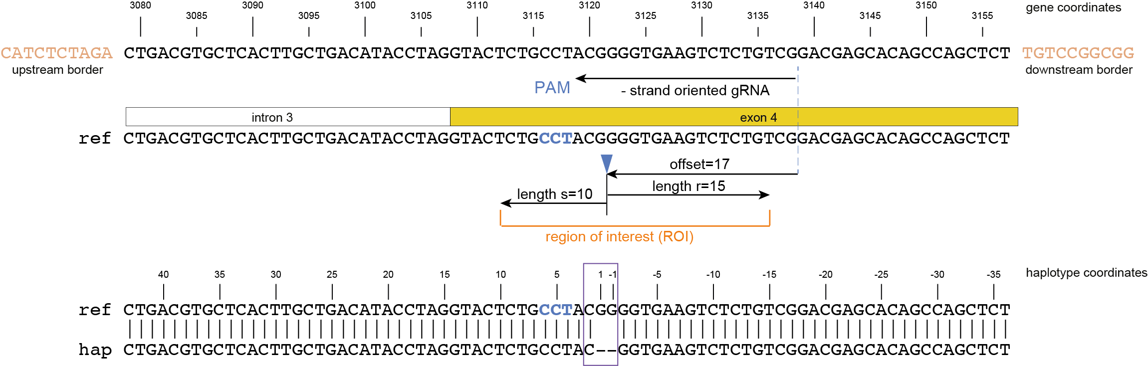
First, the gRNA location and orientation within the haplotype is retrieved from the gRNA.gff. Then, the expected cut-site is defined at distance “offset” from the 5’ start of the gRNA binding, in the direction of the PAM site (e.g. the expected Cas9 cut-site is located at distance 17 nucleotides from the 5’ start of the gRNA binding, at 3 bp before the PAM site). The user can define the offset either using the option -p , --cas_protein CAS9, which defaults to 17 bp, or adjust the offset according to the different PAM sequences in various Cas nucleases, e.g. using -f, --cas_offset 16.

CRISPR Nucleases	Organism Isolated From	PAM Sequence (5’ to 3’)
SpCas9	Streptococcus pyogenes	NGG
SaCas9	Staphylococcus aureus	NGRRT or NGRRN
NmeCas9	Neisseria meningitidis	NNNNGATT
CjCas9	Campylobacter jejuni	NNNNRYAC
StCas9	Streptococcus thermophilus	NNAGAAW
LbCpf1 (Cas12a)	Lachnospiraceae bacterium	TTTV
AsCpf1 (Cas12a)	Acidaminococcus sp.	TTTV
AacCas12b	Alicyclobacillus acidiphilus	TTN
BhCas12b v4	Bacillus hisashii	ATTN, TTTN and GTTN
Cas14	Uncultivated archea	T-rich PAM sequences, e.g. TTTA for dsDNA cleavage, no PAM sequence requirement for ssDNA
Cas3	in silico analysis of various prokaryotic genomes	No PAM sequence requirement

(source: synthego.com)

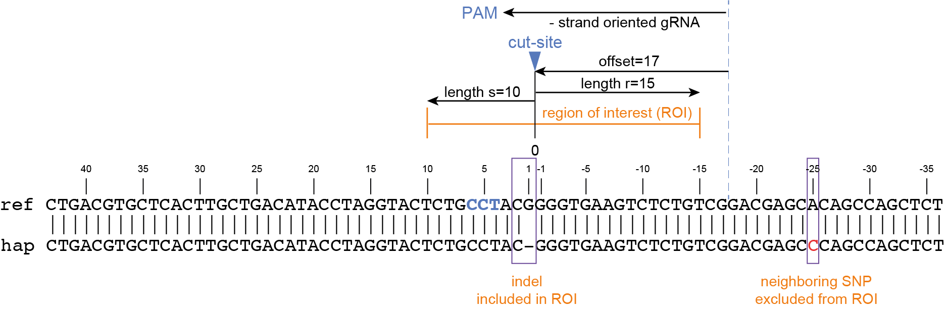
Then, using the cut-site as central point to define the region of interest (ROI), the upstream flanking region (in the direction of the PAM) is set by the parameter -s, and the downstream flanking region (in the direction of the 5’ end of the gRNA) is set by the parameter -r. If the ROI is set wide, all haplotypes that are different within the ROI will be considered unique and will not be collapsed. If the ROI is set narrow, haplotypes containing distant SNPs are collapsed with the reference haplotype in the next steps of SMAP effect-prediction as they are not considered to be caused by CRISPR/Cas activity and their effect is ignored.

Collapse haplotypes that share the same sequence in the ROI.

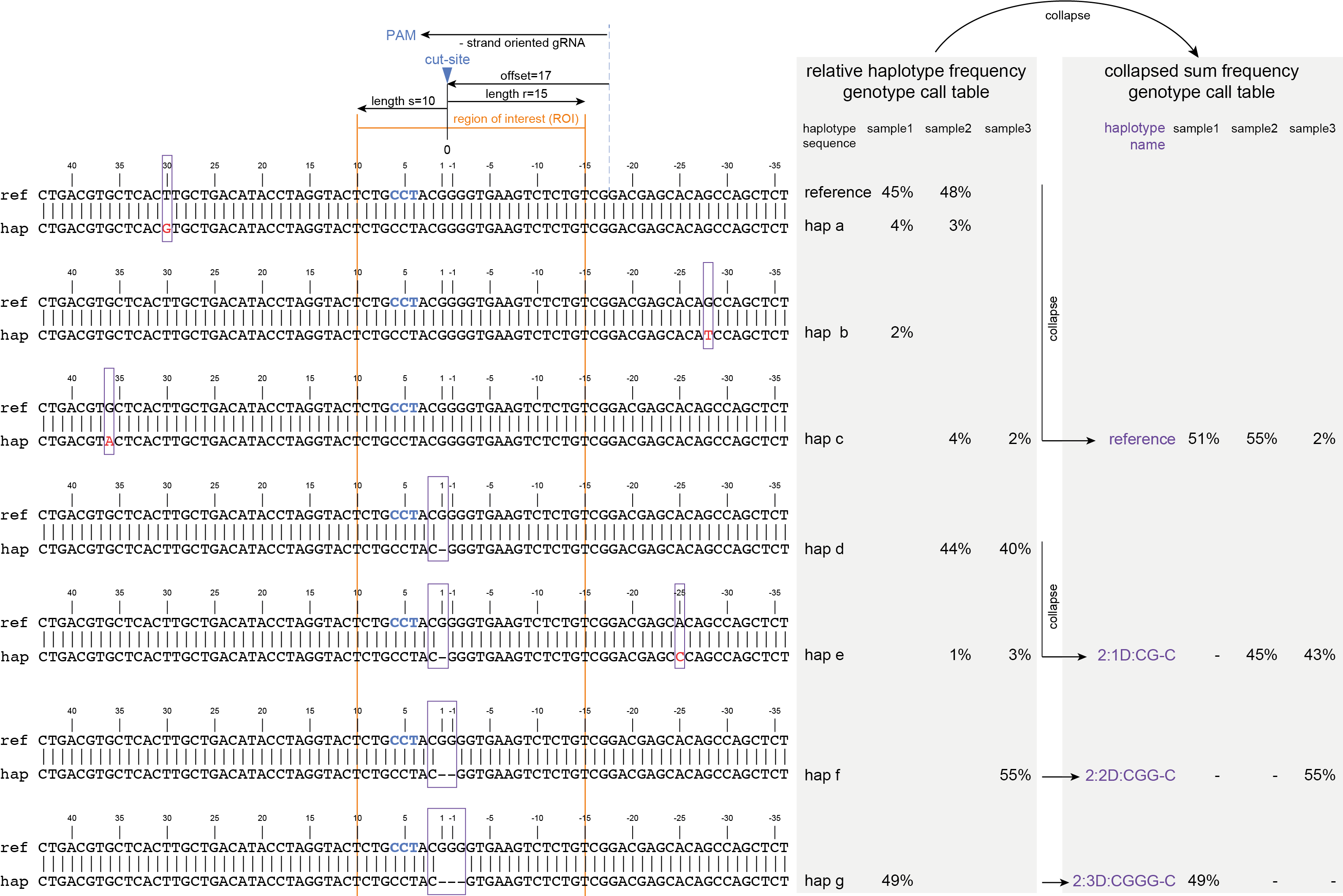
Any haplotypes that only show polymorphisms outside the ROI (a, b, c) are “collapsed” with the reference haplotype. This means that for downstream analysis, they are considered to encode the reference protein, and their relative haplotype frequency is summed with that of the reference (if any).

Any haplotypes (d, e) that share the same sequence variant overlapping with the ROI (in this case encoded by haplotype_name 2:1D:CG-C) are collapsed, independent of additional polymorphisms outside of the ROI.

Collapsing identical haplotypes (after ROI filter) means that the relative haplotype frequency is summed per sequence variant. This step ensures that read depth derived from “non-CRISPR/Cas” sequence variants is not lost; it is grouped with within haplotype sequence variants that are identical in the ROI.

This step simplifies the genotype call table as it reduces the number of unique haplotypes (from 8 to 4), and aggregates their relative haplotype frequences to reduce noise without eliminating (relative) read depth.

Annotate mutated gene model

Project mutation into the reference gene model structure.

Next, the reference sequence around the ROI is substituted by the mutated sequence, creating a new entire gene sequence. Within the haplotype sequence, only the sequence range that carries the mutation overlapping with the ROI is used for the substitution. The neighboring polymorphisms that do not overlap with the ROI themselves are not used for the substitution, so the reference gene sequence remains unchanged at those positions.

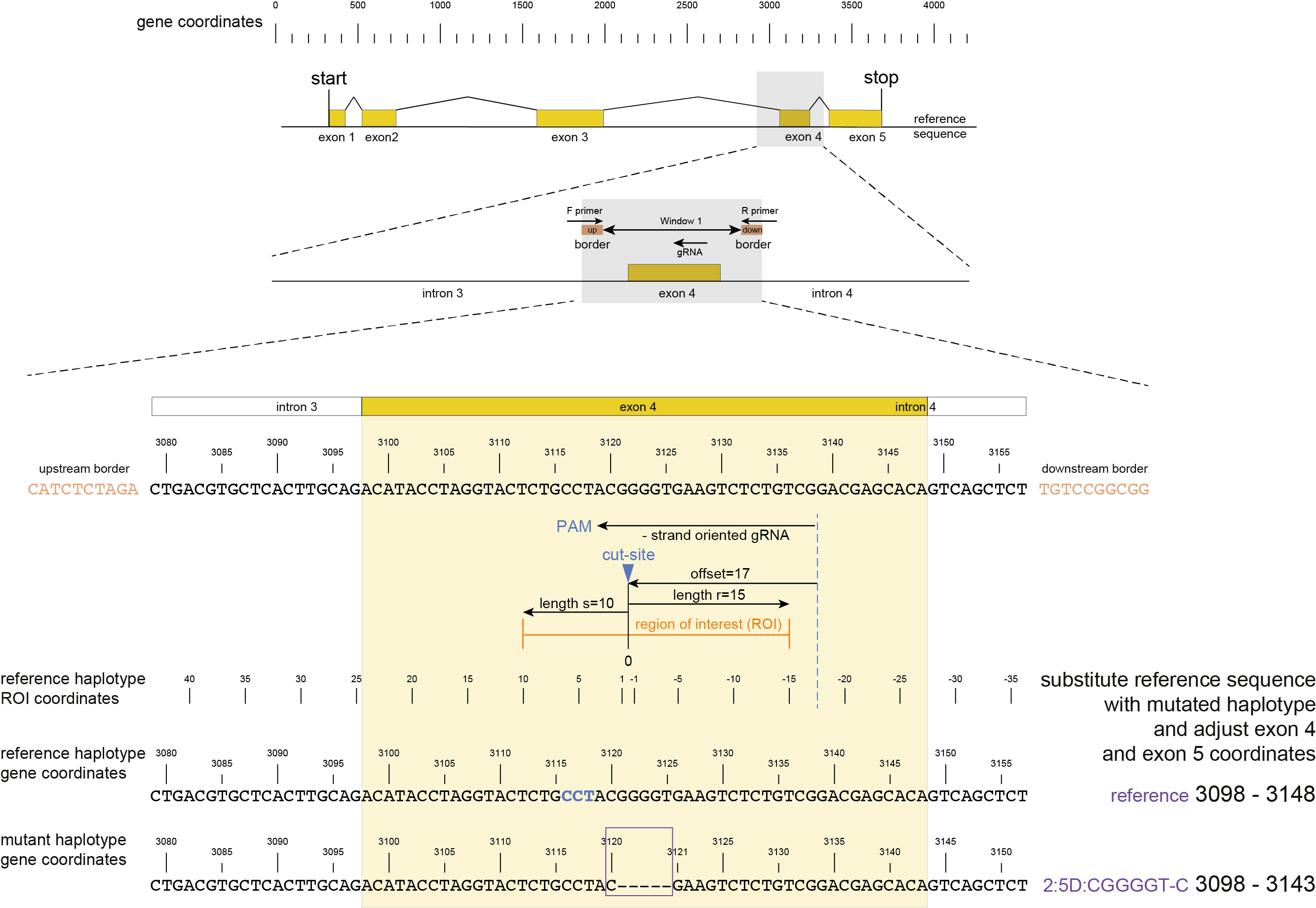
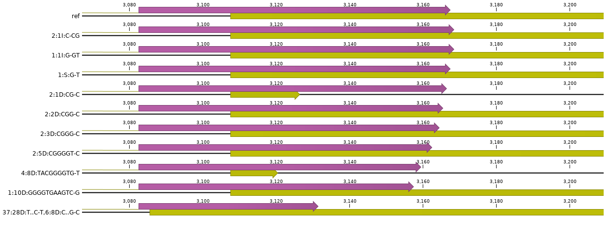
Adjust the CDS feature coordinates of the mutated gene model.

At the same time, because mutations typically include insertions or deletions, the length of the reference sequence may change, and therefore also the coordinates of all downstream gene features such as splicing donor and acceptor sites, and translational STOP codon. To keep the gene model structure correct, all CDS feature coordinates are carefully adjusted to the new reference sequence coordinates keeping local coordinates (relative to the haplotype and the ROI) in sync with global gene coordinates. If the mutation does not overlap with structural features such as translational START or STOP codons or splicing sites, then coordinates of the downstream CDS features are just shifted by the total length of the insertion or deletion.

If mutations do overlap with structural features, the CDS is changed accordingly, following common gene model prediction rationale:

• If a mutation overlaps with a translational START, the protein is considered complete loss of function (LOF, protein length = 0).

• If a mutation overlaps with a splicing donor site, the gene model is trunctated at the end of the targetted exon, or, if a splicing acceptor site is affected, at the end of the upstream exon.

• If insertions or deletions cause a frame shift and lead to a new ORF, the CDS is truncated at the first downstream translational STOP codon in the new ORF.

• If a SNP creates a novel STOP codon, the CDS is truncated there.

The result of this step is a mutated gene sequence, with positionally corrected CDS annotation that can be translated in its own open reading frame (ORF) using the initial START codon and adjusted splicing sites and STOP codon.

Translate the encoded mutated protein sequence.

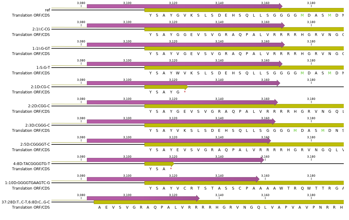
For each gene and all loci and for all unique haplotypes retained per locus after the “ROI filter and collapse” step, and after the annotation step, the corresponding full length protein sequences are translated.

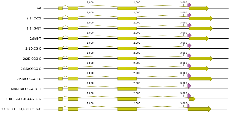
Align to the reference protein.

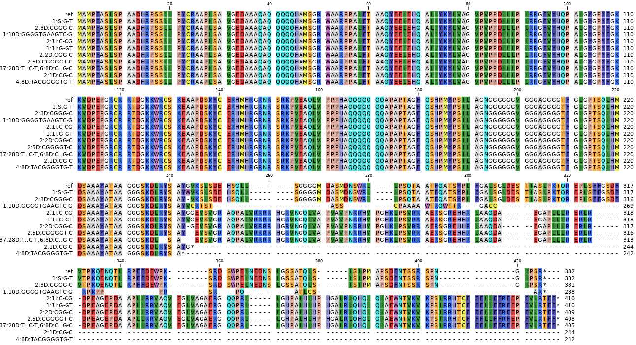
Next, each mutated protein is aligned to its corresponding reference protein in a pairwise alignment. Above, all alternative mutated proteins of gene3 are shown in a multi-sequence alignment for easier comparison of the variation in protein sequence encoded by the different haplotypes in their broader gene context.

Quantify the %identity to the reference protein and discretize to “reference” or “loss-of-function (LOF) haplotype sequences”.

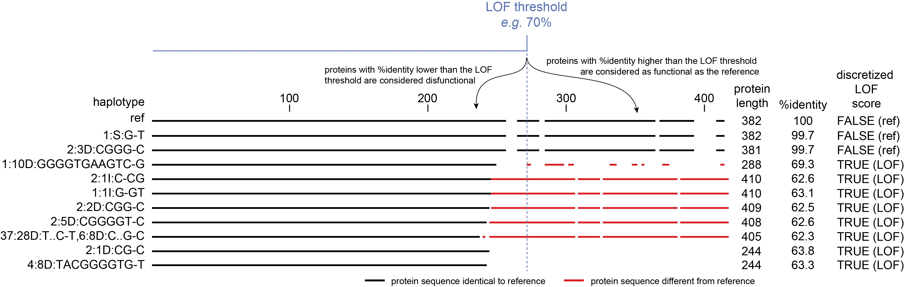
Not all edits affect the protein function, but different mutations may lead to LOF for different reasons (insertions or deletions causing frame shift, SNPs causing premature STOP codon, mutations affecting splicing sites). Since the purpose of CRISPR/Cas genome editing (in this framework anyway), is to knock out gene function, all different haplotypes causing LOF are considered equal and they can be aggregated.

Aggregate relative frequencies of LOF haplotypes

Aggregate the relative frequency of haplotypes that lead to LOF (per locus).

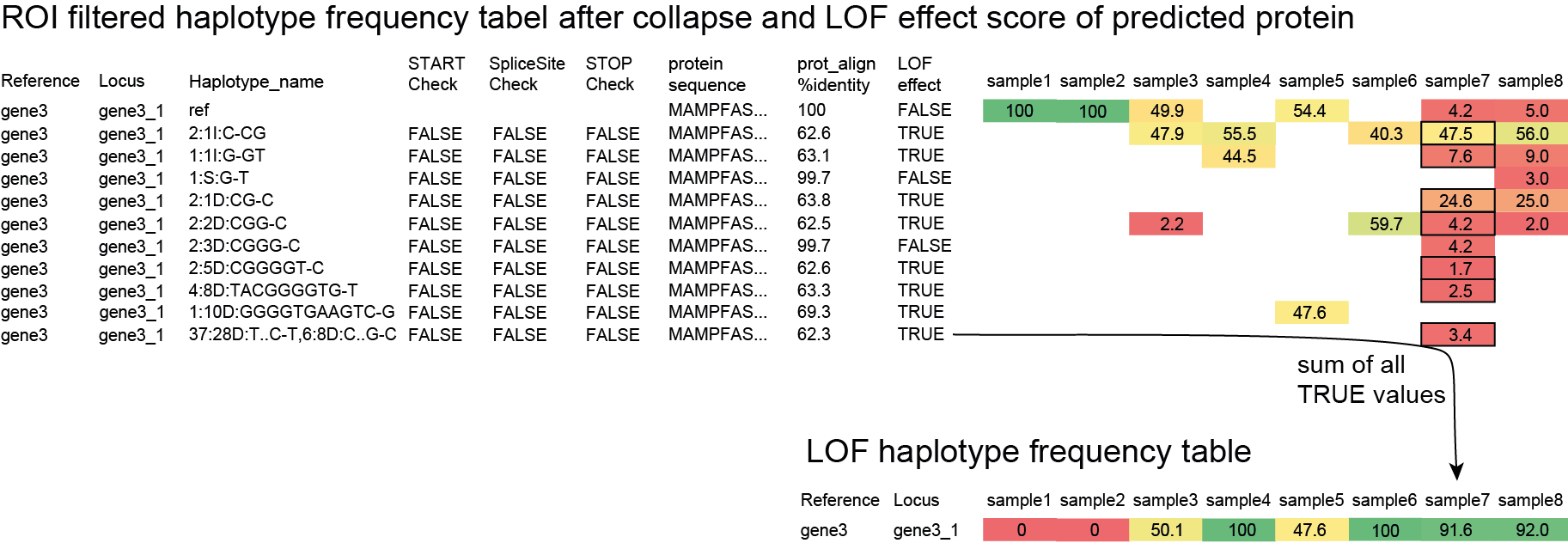
Different mutant haplotypes may lead to LOF. A plant that carries multiple LOF haplotypes is proportionally functionally impaired, even if different LOF haplotypes each only contributes a small fraction of the read depth per locus. The other haplotypes are considered as haplotypes that do not affect the encoded protein, and their summed haplotype frequencies represent the residual functional activity of the gene in the sampled tissue.

Discretize: transform to discrete LOF genotype calls

Discretize at appropriate level of protein impact.

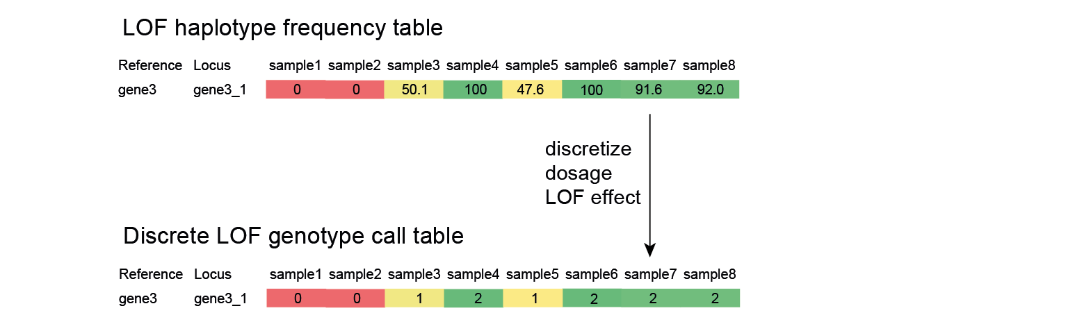
For quantitative genetic analysis based on association of bi-allelic genotype calls (ref/LOF) to quantitative phenotypic traits, a genotype call table is required that scores the discrete dosage of the LOF haplotypes per locus. Note that the bi-allelic nature of the (ref/LOF) genotype call is defined as “reference functionality” versus “loss of function, at a threshold defined as %identity of the mutated protein compared to the reference protein”.

In the SMAP effect-prediction approach, a locus is finally classified as:

• LOF dosage 0: homozygous reference if a minor fraction (<10%) of the relative read depth is taken by the cumulative read depth of all haplotypes with LOF effect on the encoded protein.

• LOF dosage 1: about half of the relative read depth (40-60%) is taken by the cumulative read depth of all haplotypes with a LOF effect on the encoded protein.

• LOF dosage 2: the majority of the relative read depth (>90%) is taken by the cumulative read depth of all haplotypes with a LOF effect on the encoded protein.

The LOF dosage can also be expressed as 0, 1, 2, 3, 4 for tetraploid organisms. The frequency interval boundaries to transform quantitative cumulative haplotype frequencies to discrete LOF dosage can be custom defined by the user.

Alternatively, the user can choose to only use the ROI filter to define haplotypes derived from CRISPR/Cas genome editing, and optionally to annotate, but not to aggregate or discretize, allowing to perform quantitative genetic analysis to associate phenotype per unique (LOF) haplotype per locus.