Recommendations & Troubleshooting
Recommendations
-partial include for GBS and Shotgun SVs and -partial exclude for HiPlex and Shotgun sliding frames.-f values to retain low-frequency haplotypes (range 1-5%) while suppressing noise.--frequency_interval_bounds, and inspect the haplotype frequency plots and then define custom thresholds if required.Why you should not run SMAP delineate on HiPlex data to identify SMAPs
Haplotyping requires the definition of a start and end point to bundle polymorphic sites. For HiPlex data, these SMAP sites are simply defined by the primer binding positions, using a Python script provided under Utilities (see further …). In GBS data and in some forms of Shotgun data (see Structural Variants), SMAPs define biologically informative sites that can be recognised (hence genotyped) based on the consistent mapping patterns at individual read level. By comparison to Shotgun and GBS data, preprocessing of HiPlex amplicon sequencing reads may be more difficult, as technical issues hamper accurate positional and pattern trimming. First, in highly multiplex amplicon sequencing, each amplicon contains a unique pair of primers. Trimming these primers off by pattern matching requires searching for all possible combinations of primers in each read, which may become computationally prohibitive. Second, as each primer typically has a slightly different length (range 18-27 bp), trimming a fixed length off the 5’-end and 3’-end of each amplicon does not yield genomic fragments with a sequence exactly internal to the primers. Third, as highly multiplex amplicon sequencing reads do not always start at the first (5’ end) nucleotide of the primer, positional trimming of reads by any fixed length would create a similar distribution of variable sequence start points, and thus artefactual Stack Mapping Anchor Points (SMAPs).
Minimum read depth filter -c
Accurate haplotype frequency estimation requires a minimum read count, which depends on sample type (individuals and Pool-Seq) and ploidy levels.
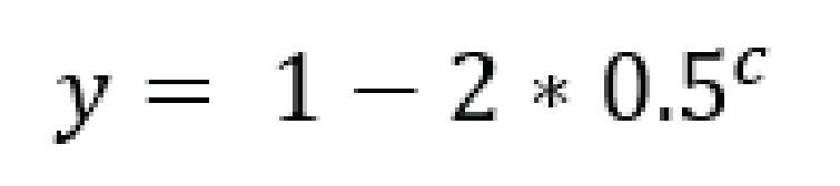
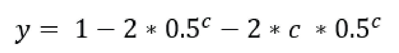
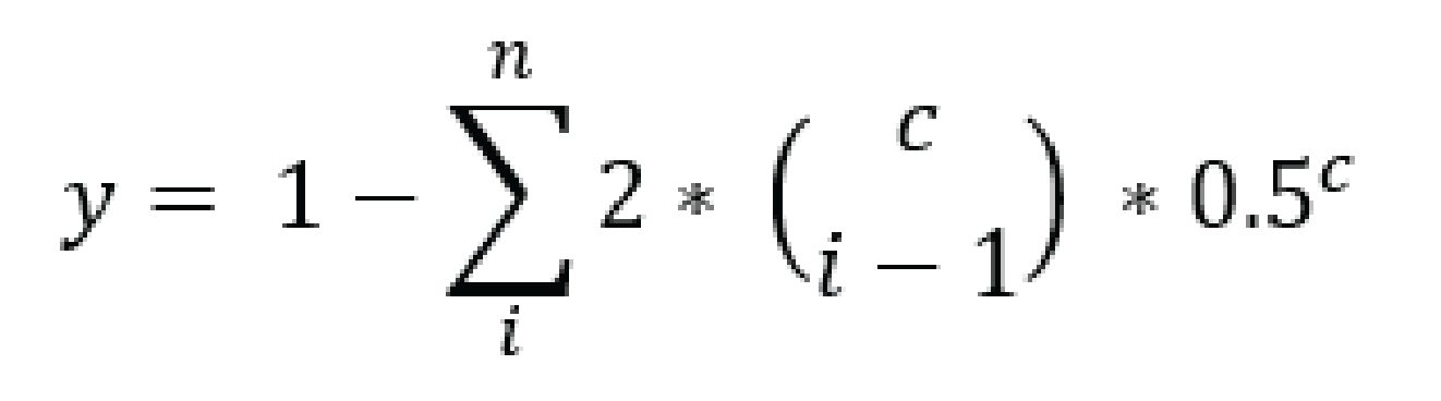
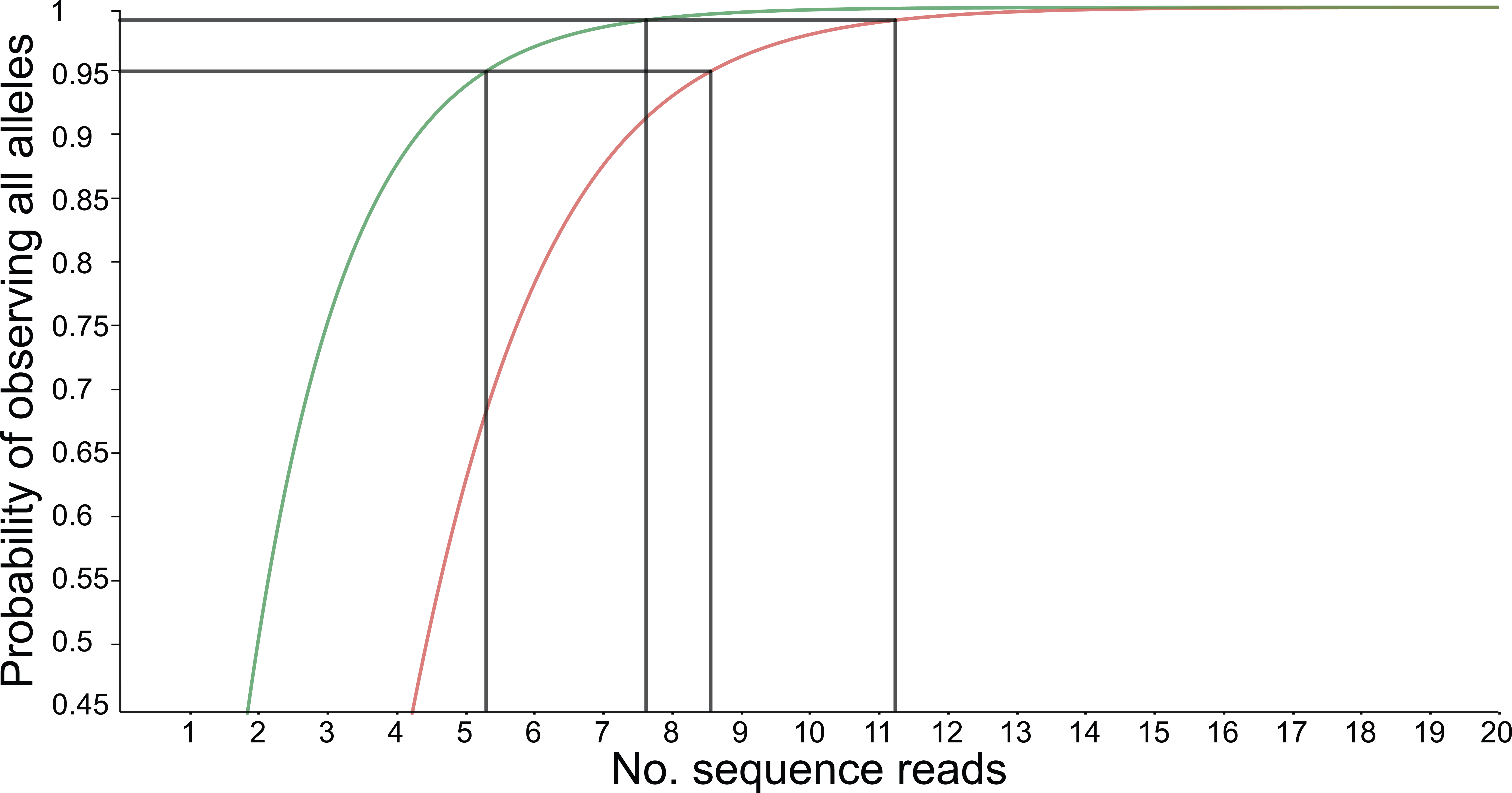
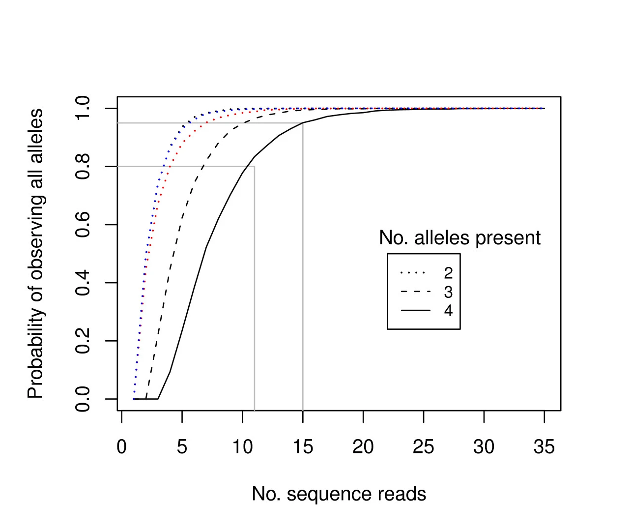
For tetraploid individuals, calculating the odds of seeing all 4 alleles at least once is a little more complicated than in diploids. A function that approximates this distribution is given by Joly et al. (2006) as
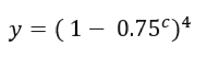
and results in a 95% chance to see all alleles at read count 15 and a 99% chance at around read count 20 (only the full black line should be considered). Figure and additional explanation Griffin et al., 2011. Just like in diploids, in order to see at least 2 copies of each allele it would be best to increase the minimal number of reads required for single copy observations.
For Pool-Seq data analysis the number of required reads depends on the ploidy as well as the number of samples in a pool, see Raineri et al. (2012), Gautier et al. (2014), and Schlötterer et al. (2014).
Therefore, the user is advised to use the read count threshold to ensure that the reported haplotype frequencies per locus are indeed based on sufficient read data. Per sample, all haplotype observations are removed for loci with a total haplotype count below the user-defined minimal read count threshold (option -c; default 0, recommended 10 for diploid individuals, 20 for tetraploid individuals, and 30 for pools).
Frequency interval bounds and dosage filter for individuals
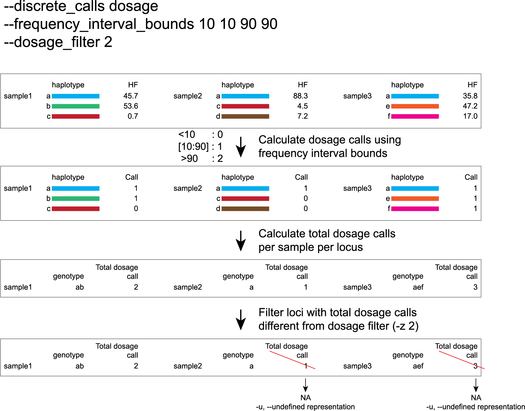
discrete dosage calls for diploids (0/1/2)
Use this option if you want to customize discrete calling thresholds. Haplotype calls with frequency below the lowerbound percentage are considered “not detected” and receive dosage `0´. Haplotype calls with a frequency between the lowerbound and the next percentage are considered heterozygous and receive haplotype dosage `1´. Haplotype calls with frequency above the upperbound percentage are considered homozygous and scored as haplotype dosage `2´. default <10, [10:90], >90 . Should be written with spaces between percentages, percentages may be written as floats or as integers [10 10 90 90].
e.g. --discrete_calls dosage --frequency_interval_bounds 10 10 90 90 translates to: haplotype frequency < 10% = 0, haplotype frequency > 10% & < 90% = 1, haplotype frequency > 90% = 2.
Visualized examples of these thresholds can be found in these tabs.
discrete dominant calls for diploids (0/1)
Lowerbound frequency for dominant call haplotypes. Haplotypes with frequency above this percentage are scored as dominant present haplotype [10].
e.g. --discrete_calls dominant --frequency_interval_bounds 10 translates to: haplotype frequency < 10% = 0, haplotype frequency > 10% = 1
Visualized examples of these thresholds can be found in these tabs.
discrete dosage calls for tetraploids (0/1/2/3/4)
Use this option if you want to customize discrete calling thresholds, haplotype calls with frequency below the lowerbound percentage are considered not detected and receive dosage `0´ . Haplotype calls with frequency between the lowerbound and next percentage are considered present in 1 out of 4 alleles and scored as haplotype dosage `1´ , haplotype frequencies in the next frequency interval are scored as haplotype dosage `2´ , and so on. Haplotype calls with frequency above the upperbound percentage are considered homozygous and scored as haplotype dosage `4´ default <12.5, [12.5:37.5], [37.5:62.5], [62.5:87.5], >87.5 . Should be written with spaces between percentages, percentages may be written as floats or as integers [12.5 12.5 37.5 37.5 62.5 62.5 87.5 87.5].
e.g. --discrete_calls dosage --frequency_interval_bounds 12.5 12.5 37.5 37.5 62.5 62.5 87.5 87.5 translates to: haplotype frequency < 12.5% = 0, haplotype frequency > 12.5% & < 37.5% = 1, haplotype frequency > 37.5.5% & < 62.5% = 2, haplotype frequency > 62.5% & < 87.5% = 3, haplotype frequency > 87.5% = 4.
Visualized examples of these thresholds can be found in these tabs.
discrete dominant calls for tetraploids (0/1)
Lowerbound frequency for dominant call haplotypes. Haplotypes with frequency above this percentage are scored as dominant present haplotype [10].
e.g. --discrete_calls dominant --frequency_interval_bounds 10 translates to: haplotype frequency < 10% = 0, haplotype frequency > 10% = 1.
Visualized examples of these thresholds can be found in these tabs.
Why use dosage filter to remove low quality genotype calls (-z)?
The dosage filter -z is an additional mask specifically for dosage calls in individuals. It masks loci within samples from the dataset (replaced by -u or --undefined_representation) based on total dosage calls (= total allele count calculated from haplotype frequencies using frequency interval bounds).
It is important to distinguish between total dosage call and total number of unique alleles per locus per sample.
A tetraploid individual for example is expected to contain a total dosage call of 4 alleles, but can contain from 1 up to 4 unique (different) alleles:
locus |
dosage |
total dosage call |
number of unique alleles |
|||
|---|---|---|---|---|---|---|
. |
a |
b |
c |
d |
. |
. |
aaaa |
4 |
0 |
0 |
0 |
4 |
1 |
aaab |
3 |
1 |
0 |
0 |
4 |
2 |
aabb |
2 |
2 |
0 |
0 |
4 |
2 |
abcc |
1 |
1 |
2 |
0 |
4 |
3 |
abcd |
1 |
1 |
1 |
1 |
4 |
4 |
The dosage filter -z evaluates the total dosage call against the expected number of alleles (2 in diploids, 4 in tetraploids), but does not consider the number of unique alleles. In general, the expected total dosage call for any locus is equal to the ploidy of the individual (except in exceptional cases such as aneuploidy).
Consider the examples of a single locus in a few samples in the tabs below for illustration of the combined functions of -f (minimum haplotype frequency), --frequency_interval_bounds and -z (dosage_mask).
-f (minimum haplotype frequency) is especially useful to reduce the number of masked calls across the sample set.-f, also means removing the associated read counts from the read count table and recalculating the relative frequencies of the other haplotype based on the remaining read counts.--frequency_interval_bounds can be adjusted by the user, based on the haplotype frequency distribution plot. Lowerbound and upperbound thresholds should be set to remove the extremes in the haplotype frequency graphs, to reduce noise before discrete genotype calling and masking.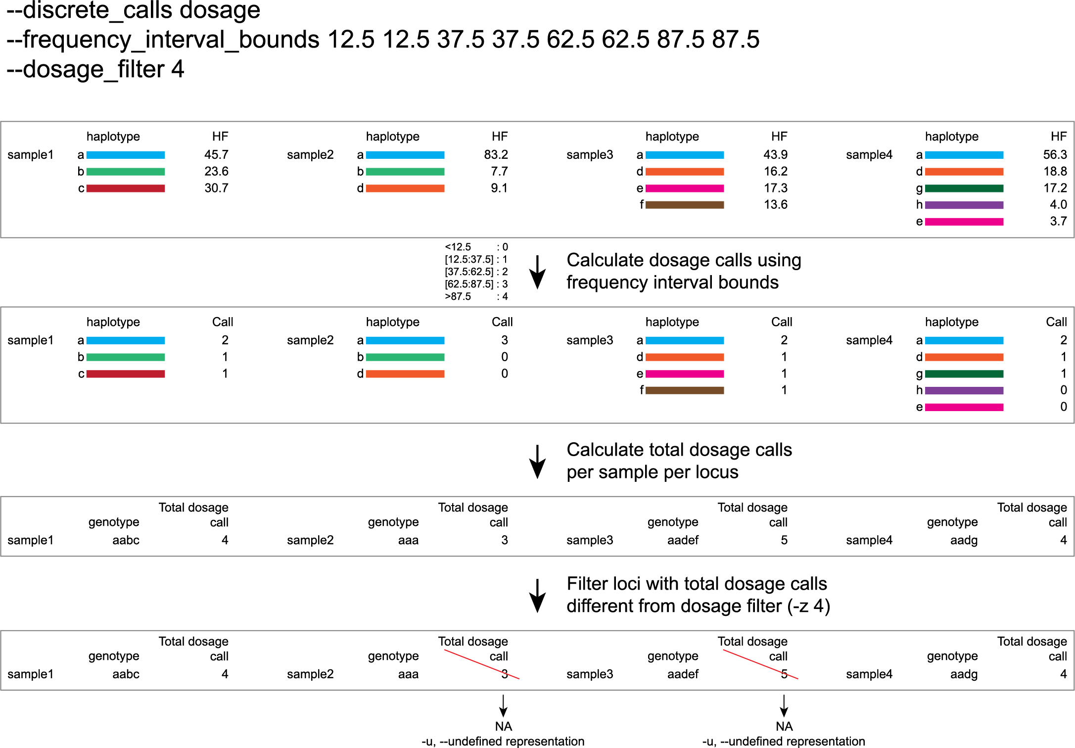
Troubleshooting
Output
When opening the output (Tab delimited) .tsv files in Microsoft Excel, one might encounter the error that certain rows contain 1 column and others 2 columns, making it impossible to use the built-in option Data -> Text to Columns. In order to circumvent this issue, it is best to open a new Excel-file and use the option Data -> Get Data -> From Text/CSV.