Individuals
Step 4: Filtering haplotypes and calculating haplotype frequencies
procedure
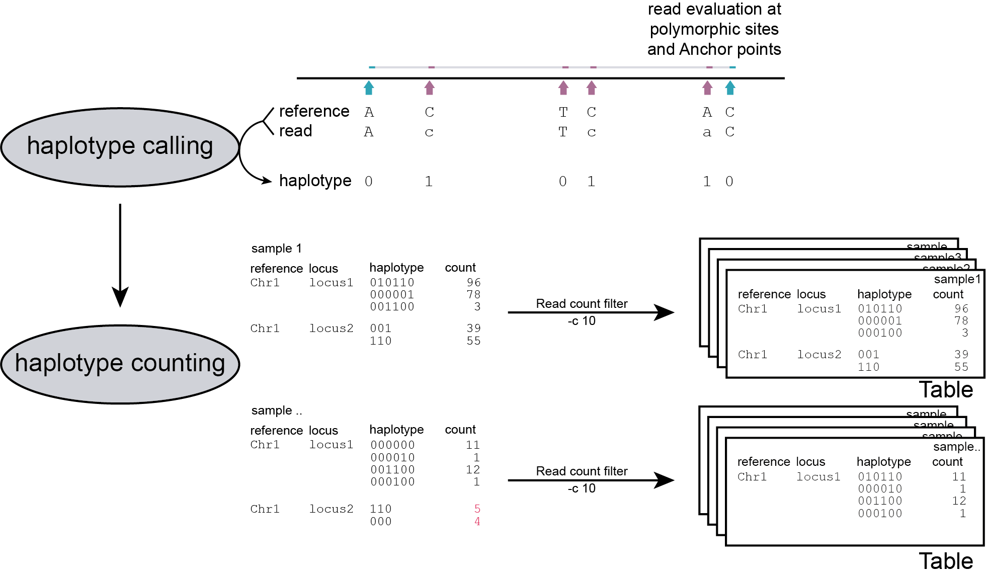
After processing all BAM files in the given directory and storing all observed haplotypes in a table for each sample, SMAP haplotype-sites loops over all tables to create an integrated genotyping matrix that contains all observed haplotypes across all BAM files and collects their absolute read counts. The next step is to switch from absolute read count per haplotype to relative read depth per haplotype per locus, i.e. to calculate haplotype frequencies. The haplotype frequency is calculated per haplotype per locus per sample (haplotype count per sample/total read count per locus per sample; range 0-100%).
filters
Randomly distributed read errors that happen to co-localize with the SMAP/SNP positions erroneously create low frequency haplotypes. Example data are shown in the scheme above, see tables below for the occurence in real GBS data of 8 diploid individuals.
-f
Haplotypes that never reach a user-defined minimum haplotype frequency threshold (default 0%) in at least one of the samples, are removed entirely from the haplotype count table. After this filter, the haplotype frequency is recalculated on the remaining read counts per haplotype per locus per sample. The effect of adjusting this filter is illustrated in real data in the tables below. Please compare the tables below at subsequent steps of filtering: -f 0 filtering is effectively no filter (all haplotype observations > 0% are kept). Most noise from low frequency haplotypes can effectively be removed with -f 1 or -f 5 . We recommend to test the effect of this parameter on your own data, and to inspect the haplotype frequency histograms generated (see Graphical output).
-m
Haplotypes that reach the user defined -f value in at least one BAM file are retained. However, observations of the same haplotype in other BAM files but with a haplotype frequency lower than the -f value are also retained, potentially allowing noise. These values may additionaly be masked with option -m.
The option -m masks all haplotype frequencies lower than set value by substituting them with NaN’s or another value defined by --undefined_representation. The other haplotype frequencies are not recalculated.
The following tabs show real experimental data of two loci. All detected haplotypes are reported using the default -f 0, demonstrating how haplotype frequency filtering removes noise.
Locus |
haplotype |
2n_ind_GBS-SE_001.bam |
2n_ind_GBS-SE_002.bam |
2n_ind_GBS-SE_003.bam |
2n_ind_GBS-SE_004.bam |
2n_ind_GBS-SE_005.bam |
2n_ind_GBS-SE_006.bam |
2n_ind_GBS-SE_007.bam |
2n_ind_GBS-SE_008.bam |
|---|---|---|---|---|---|---|---|---|---|
Chrom_1:15618-15711_+ |
…..0100001 |
0.00 |
1.03 |
0.00 |
0.00 |
0.00 |
0.00 |
0.00 |
0.00 |
Chrom_1:15618-15711_+ |
…000000… |
0.00 |
0.00 |
0.00 |
0.00 |
0.18 |
0.48 |
0.00 |
0.00 |
Chrom_1:15618-15711_+ |
…000000000 |
0.00 |
0.00 |
0.00 |
0.00 |
0.00 |
0.00 |
3.05 |
0.98 |
Chrom_1:15618-15711_+ |
…000010000 |
0.22 |
0.00 |
0.00 |
0.00 |
0.00 |
0.00 |
0.00 |
0.00 |
Chrom_1:15618-15711_+ |
…001010110 |
0.00 |
0.00 |
0.00 |
0.93 |
0.00 |
0.00 |
0.00 |
0.00 |
Chrom_1:15618-15711_+ |
…010000000 |
0.00 |
0.00 |
0.00 |
0.00 |
0.70 |
0.00 |
0.00 |
0.98 |
Chrom_1:15618-15711_+ |
.010000….. |
0.00 |
0.00 |
0.00 |
0.93 |
0.00 |
0.00 |
2.44 |
1.96 |
Chrom_1:15618-15711_+ |
.01000000000 |
41.87 |
0.00 |
0.00 |
0.00 |
0.00 |
1.43 |
91.46 |
3.92 |
Chrom_1:15618-15711_+ |
.01000000010 |
0.22 |
0.00 |
0.00 |
0.00 |
0.00 |
0.00 |
0.00 |
0.00 |
Chrom_1:15618-15711_+ |
.01000100000 |
0.22 |
46.39 |
0.00 |
0.00 |
0.00 |
0.00 |
1.22 |
0.00 |
Chrom_1:15618-15711_+ |
.010010….. |
0.00 |
0.00 |
0.00 |
0.93 |
0.00 |
0.00 |
0.00 |
0.00 |
Chrom_1:15618-15711_+ |
.01001000000 |
0.22 |
0.00 |
0.00 |
0.00 |
0.00 |
0.00 |
0.00 |
0.00 |
Chrom_1:15618-15711_+ |
.01001010110 |
0.00 |
0.00 |
0.00 |
81.48 |
0.00 |
0.00 |
0.00 |
0.00 |
Chrom_1:15618-15711_+ |
.010100….. |
0.00 |
0.00 |
0.00 |
0.00 |
0.00 |
0.00 |
0.00 |
0.98 |
Chrom_1:15618-15711_+ |
.0101000000. |
0.00 |
0.00 |
0.00 |
0.00 |
0.18 |
0.00 |
0.00 |
0.00 |
Chrom_1:15618-15711_+ |
.01010000000 |
0.00 |
0.00 |
0.00 |
0.00 |
48.95 |
0.48 |
0.61 |
84.31 |
Chrom_1:15618-15711_+ |
.01100000000 |
0.00 |
0.00 |
45.68 |
0.00 |
0.00 |
0.00 |
0.00 |
0.00 |
Chrom_1:15618-15711_+ |
.01110000000 |
0.00 |
0.00 |
0.82 |
0.00 |
0.00 |
0.00 |
0.00 |
0.00 |
Chrom_1:15618-15711_+ |
0000000….. |
0.22 |
0.00 |
0.00 |
0.00 |
0.00 |
0.00 |
0.00 |
0.00 |
Chrom_1:15618-15711_+ |
00000000…. |
0.00 |
0.00 |
0.00 |
0.00 |
0.00 |
0.48 |
0.00 |
0.00 |
Chrom_1:15618-15711_+ |
000000000… |
55.23 |
49.48 |
53.50 |
15.74 |
48.95 |
95.24 |
1.22 |
6.86 |
Chrom_1:15618-15711_+ |
0000000000.. |
0.00 |
1.03 |
0.00 |
0.00 |
0.18 |
0.00 |
0.00 |
0.00 |
Chrom_1:15618-15711_+ |
000000010… |
0.45 |
0.00 |
0.00 |
0.00 |
0.00 |
0.00 |
0.00 |
0.00 |
Chrom_1:15618-15711_+ |
000000100… |
0.22 |
0.00 |
0.00 |
0.00 |
0.00 |
0.00 |
0.00 |
0.00 |
Chrom_1:15618-15711_+ |
000001000… |
0.00 |
0.00 |
0.00 |
0.00 |
0.18 |
0.48 |
0.00 |
0.00 |
Chrom_1:15618-15711_+ |
000010000… |
0.00 |
1.03 |
0.00 |
0.00 |
0.00 |
1.43 |
0.00 |
0.00 |
Chrom_1:15618-15711_+ |
000011000… |
0.00 |
0.00 |
0.00 |
0.00 |
0.18 |
0.00 |
0.00 |
0.00 |
Chrom_1:15618-15711_+ |
000100000… |
0.89 |
0.00 |
0.00 |
0.00 |
0.18 |
0.00 |
0.00 |
0.00 |
Chrom_1:15618-15711_+ |
010000000… |
0.00 |
0.00 |
0.00 |
0.00 |
0.35 |
0.00 |
0.00 |
0.00 |
Chrom_1:15618-15711_+ |
010010000… |
0.22 |
0.00 |
0.00 |
0.00 |
0.00 |
0.00 |
0.00 |
0.00 |
Chrom_1:15618-15711_+ |
100000000… |
0.00 |
1.03 |
0.00 |
0.00 |
0.00 |
0.00 |
0.00 |
0.00 |
Chrom_1:15713-15798_- |
..000000 |
0.00 |
0.00 |
0.00 |
0.00 |
0.15 |
0.00 |
0.00 |
0.00 |
Chrom_1:15713-15798_- |
.0000000 |
0.22 |
0.00 |
0.00 |
0.00 |
0.15 |
0.48 |
0.00 |
0.00 |
Chrom_1:15713-15798_- |
.1111010 |
0.00 |
0.00 |
0.00 |
0.00 |
0.15 |
0.00 |
0.00 |
0.00 |
Chrom_1:15713-15798_- |
0000…. |
0.00 |
0.00 |
0.00 |
0.00 |
0.00 |
0.48 |
0.00 |
0.00 |
Chrom_1:15713-15798_- |
00000000 |
61.88 |
63.77 |
51.54 |
26.37 |
52.75 |
94.23 |
1.48 |
5.15 |
Chrom_1:15713-15798_- |
00000001 |
0.00 |
0.00 |
0.38 |
0.00 |
0.00 |
0.00 |
0.00 |
0.00 |
Chrom_1:15713-15798_- |
00000100 |
0.00 |
0.00 |
0.00 |
0.00 |
0.00 |
0.48 |
0.00 |
0.00 |
Chrom_1:15713-15798_- |
00001… |
0.00 |
0.00 |
0.00 |
0.00 |
0.00 |
0.00 |
0.00 |
1.03 |
Chrom_1:15713-15798_- |
000010.. |
0.00 |
0.00 |
0.00 |
3.30 |
0.00 |
0.00 |
0.00 |
3.09 |
Chrom_1:15713-15798_- |
00001000 |
0.00 |
0.00 |
0.77 |
0.00 |
0.31 |
0.00 |
0.00 |
0.00 |
Chrom_1:15713-15798_- |
00010000 |
0.00 |
0.00 |
0.00 |
0.00 |
0.31 |
0.96 |
0.00 |
0.00 |
Chrom_1:15713-15798_- |
00100000 |
0.00 |
0.00 |
0.38 |
0.00 |
0.00 |
0.00 |
0.00 |
0.00 |
Chrom_1:15713-15798_- |
001010.. |
0.00 |
0.00 |
0.00 |
0.00 |
0.00 |
0.00 |
0.00 |
1.03 |
Chrom_1:15713-15798_- |
0100…. |
0.00 |
0.00 |
0.00 |
2.20 |
0.00 |
0.00 |
0.00 |
0.00 |
Chrom_1:15713-15798_- |
01000000 |
0.00 |
0.00 |
0.00 |
0.00 |
0.15 |
0.48 |
0.00 |
0.00 |
Chrom_1:15713-15798_- |
010010.. |
0.00 |
0.00 |
0.00 |
68.13 |
0.00 |
0.00 |
0.00 |
0.00 |
Chrom_1:15713-15798_- |
011….. |
0.00 |
0.00 |
0.00 |
0.00 |
0.00 |
0.00 |
0.00 |
1.03 |
Chrom_1:15713-15798_- |
0111…. |
0.00 |
0.00 |
0.38 |
0.00 |
0.15 |
0.00 |
0.00 |
0.00 |
Chrom_1:15713-15798_- |
01110010 |
0.22 |
0.00 |
0.38 |
0.00 |
0.31 |
0.00 |
0.00 |
0.00 |
Chrom_1:15713-15798_- |
011110.. |
0.00 |
0.00 |
0.38 |
0.00 |
0.31 |
0.00 |
0.74 |
2.06 |
Chrom_1:15713-15798_- |
01111000 |
0.00 |
0.00 |
0.00 |
0.00 |
0.00 |
0.00 |
0.00 |
1.03 |
Chrom_1:15713-15798_- |
01111010 |
37.44 |
36.23 |
45.77 |
0.00 |
45.26 |
2.88 |
96.30 |
85.57 |
Chrom_1:15713-15798_- |
01111110 |
0.22 |
0.00 |
0.00 |
0.00 |
0.00 |
0.00 |
0.74 |
0.00 |
Chrom_1:15713-15798_- |
11111010 |
0.00 |
0.00 |
0.00 |
0.00 |
0.00 |
0.00 |
0.74 |
0.00 |
Locus |
haplotype |
2n_ind_GBS-SE_001.bam |
2n_ind_GBS-SE_002.bam |
2n_ind_GBS-SE_003.bam |
2n_ind_GBS-SE_004.bam |
2n_ind_GBS-SE_005.bam |
2n_ind_GBS-SE_006.bam |
2n_ind_GBS-SE_007.bam |
2n_ind_GBS-SE_008.bam |
|---|---|---|---|---|---|---|---|---|---|
Chrom_1:15618-15711_+ |
…..0100001 |
0.00 |
1.03 |
0.00 |
0.00 |
0.00 |
0.00 |
0.00 |
0.00 |
Chrom_1:15618-15711_+ |
…000000000 |
0.00 |
0.00 |
0.00 |
0.00 |
0.00 |
0.00 |
3.05 |
1.00 |
Chrom_1:15618-15711_+ |
.010000….. |
0.00 |
0.00 |
0.00 |
0.94 |
0.00 |
0.00 |
2.44 |
2.00 |
Chrom_1:15618-15711_+ |
.01000000000 |
43.02 |
0.00 |
0.00 |
0.00 |
0.00 |
1.45 |
91.46 |
4.00 |
Chrom_1:15618-15711_+ |
.01000100000 |
0.23 |
46.39 |
0.00 |
0.00 |
0.00 |
0.00 |
1.22 |
0.00 |
Chrom_1:15618-15711_+ |
.01001010110 |
0.00 |
0.00 |
0.00 |
83.02 |
0.00 |
0.00 |
0.00 |
0.00 |
Chrom_1:15618-15711_+ |
.01010000000 |
0.00 |
0.00 |
0.00 |
0.00 |
49.91 |
0.48 |
0.61 |
86.00 |
Chrom_1:15618-15711_+ |
.01100000000 |
0.00 |
0.00 |
46.06 |
0.00 |
0.00 |
0.00 |
0.00 |
0.00 |
Chrom_1:15618-15711_+ |
000000000… |
56.75 |
49.48 |
53.94 |
16.04 |
49.91 |
96.62 |
1.22 |
7.00 |
Chrom_1:15618-15711_+ |
0000000000.. |
0.00 |
1.03 |
0.00 |
0.00 |
0.18 |
0.00 |
0.00 |
0.00 |
Chrom_1:15618-15711_+ |
000010000… |
0.00 |
1.03 |
0.00 |
0.00 |
0.00 |
1.45 |
0.00 |
0.00 |
Chrom_1:15618-15711_+ |
100000000… |
0.00 |
1.03 |
0.00 |
0.00 |
0.00 |
0.00 |
0.00 |
0.00 |
Chrom_1:15713-15798_- |
00000000 |
62.3 |
63.77 |
52.76 |
26.37 |
53.65 |
97.03 |
1.5 |
5.15 |
Chrom_1:15713-15798_- |
00001… |
0.00 |
0.00 |
0.00 |
0.00 |
0.00 |
0.00 |
0.00 |
1.03 |
Chrom_1:15713-15798_- |
000010.. |
0.00 |
0.00 |
0.00 |
3.3 |
0.00 |
0.00 |
0.00 |
3.09 |
Chrom_1:15713-15798_- |
001010.. |
0.00 |
0.00 |
0.00 |
0.00 |
0.00 |
0.00 |
0.00 |
1.03 |
Chrom_1:15713-15798_- |
0100…. |
0.00 |
0.00 |
0.00 |
2.2 |
0.00 |
0.00 |
0.00 |
0.00 |
Chrom_1:15713-15798_- |
010010.. |
0.00 |
0.00 |
0.00 |
68.13 |
0.00 |
0.00 |
0.00 |
0.00 |
Chrom_1:15713-15798_- |
011….. |
0.00 |
0.00 |
0.00 |
0.00 |
0.00 |
0.00 |
0.00 |
1.03 |
Chrom_1:15713-15798_- |
011110.. |
0.00 |
0.00 |
0.39 |
0.00 |
0.31 |
0.00 |
0.75 |
2.06 |
Chrom_1:15713-15798_- |
01111000 |
0.00 |
0.00 |
0.00 |
0.00 |
0.00 |
0.00 |
0.00 |
1.03 |
Chrom_1:15713-15798_- |
01111010 |
37.7 |
36.23 |
46.85 |
0.00 |
46.03 |
2.97 |
97.74 |
85.57 |
Locus |
haplotype |
2n_ind_GBS-SE_001.bam |
2n_ind_GBS-SE_002.bam |
2n_ind_GBS-SE_003.bam |
2n_ind_GBS-SE_004.bam |
2n_ind_GBS-SE_005.bam |
2n_ind_GBS-SE_006.bam |
2n_ind_GBS-SE_007.bam |
2n_ind_GBS-SE_008.bam |
|---|---|---|---|---|---|---|---|---|---|
Chrom_1:15618-15711_+ |
.01000000000 |
43.02 |
0.00 |
0.00 |
0.00 |
0.00 |
1.47 |
96.77 |
4.12 |
Chrom_1:15618-15711_+ |
.01000100000 |
0.23 |
48.39 |
0.00 |
0.00 |
0.00 |
0.00 |
1.29 |
0.00 |
Chrom_1:15618-15711_+ |
.01001010110 |
0.00 |
0.00 |
0.00 |
83.81 |
0.00 |
0.00 |
0.00 |
0.00 |
Chrom_1:15618-15711_+ |
.01010000000 |
0.00 |
0.00 |
0.00 |
0.00 |
50.00 |
0.49 |
0.65 |
88.66 |
Chrom_1:15618-15711_+ |
.01100000000 |
0.00 |
0.00 |
46.06 |
0.00 |
0.00 |
0.00 |
0.00 |
0.00 |
Chrom_1:15618-15711_+ |
000000000… |
56.75 |
51.61 |
53.94 |
16.19 |
50.00 |
98.04 |
1.29 |
7.22 |
Chrom_1:15713-15798_- |
00000000 |
62.30 |
63.77 |
52.96 |
27.91 |
53.82 |
97.03 |
1.52 |
5.68 |
Chrom_1:15713-15798_- |
010010.. |
0.00 |
0.00 |
0.00 |
72.09 |
0.00 |
0.00 |
0.00 |
0.00 |
Chrom_1:15713-15798_- |
01111010 |
37.70 |
36.23 |
47.04 |
0.00 |
46.18 |
2.97 |
98.48 |
94.32 |
Locus |
haplotype |
2n_ind_GBS-SE_001.bam |
2n_ind_GBS-SE_002.bam |
2n_ind_GBS-SE_003.bam |
2n_ind_GBS-SE_004.bam |
2n_ind_GBS-SE_005.bam |
2n_ind_GBS-SE_006.bam |
2n_ind_GBS-SE_007.bam |
2n_ind_GBS-SE_008.bam |
|---|---|---|---|---|---|---|---|---|---|
Chrom_1:15618-15711_+ |
.01000000000 |
43.02 |
0.00 |
0.00 |
0.00 |
0.00 |
1.47 |
96.77 |
4.12 |
Chrom_1:15618-15711_+ |
.01000100000 |
NA |
48.39 |
0.00 |
0.00 |
0.00 |
0.00 |
1.29 |
0.00 |
Chrom_1:15618-15711_+ |
.01001010110 |
0.00 |
0.00 |
0.00 |
83.81 |
0.00 |
0.00 |
0.00 |
0.00 |
Chrom_1:15618-15711_+ |
.01010000000 |
0.00 |
0.00 |
0.00 |
0.00 |
50.00 |
NA |
0.00 |
88.66 |
Chrom_1:15618-15711_+ |
.01100000000 |
0.00 |
0.00 |
46.06 |
0.00 |
0.00 |
0.00 |
0.00 |
0.00 |
Chrom_1:15618-15711_+ |
000000000… |
56.75 |
51.61 |
53.94 |
16.19 |
50.00 |
98.04 |
1.29 |
7.22 |
Chrom_1:15713-15798_- |
00000000 |
62.30 |
63.77 |
52.96 |
27.91 |
53.82 |
97.03 |
1.52 |
5.68 |
Chrom_1:15713-15798_- |
010010.. |
0.00 |
0.00 |
0.00 |
72.09 |
0.00 |
0.00 |
0.00 |
0.00 |
Chrom_1:15713-15798_- |
01111010 |
37.70 |
36.23 |
47.04 |
0.00 |
46.18 |
2.97 |
98.48 |
94.32 |
Locus |
haplotype |
2n_ind_GBS-SE_001.bam |
2n_ind_GBS-SE_002.bam |
2n_ind_GBS-SE_003.bam |
2n_ind_GBS-SE_004.bam |
2n_ind_GBS-SE_005.bam |
2n_ind_GBS-SE_006.bam |
2n_ind_GBS-SE_007.bam |
2n_ind_GBS-SE_008.bam |
|---|---|---|---|---|---|---|---|---|---|
Chrom_1:15618-15711_+ |
.01000000000 |
43.02 |
0.00 |
0.00 |
0.00 |
0.00 |
NA |
96.77 |
NA |
Chrom_1:15618-15711_+ |
.01000100000 |
NA |
48.39 |
0.00 |
0.00 |
0.00 |
0.00 |
NA |
0.00 |
Chrom_1:15618-15711_+ |
.01001010110 |
0.00 |
0.00 |
0.00 |
83.81 |
0.00 |
0.00 |
0.00 |
0.00 |
Chrom_1:15618-15711_+ |
.01010000000 |
0.00 |
0.00 |
0.00 |
0.00 |
50.00 |
NA |
0.00 |
88.66 |
Chrom_1:15618-15711_+ |
.01100000000 |
0.00 |
0.00 |
46.06 |
0.00 |
0.00 |
0.00 |
0.00 |
0.00 |
Chrom_1:15618-15711_+ |
000000000… |
56.75 |
51.61 |
53.94 |
16.19 |
50.00 |
98.04 |
NA |
7.22 |
Chrom_1:15713-15798_- |
00000000 |
62.30 |
63.77 |
52.96 |
27.91 |
53.82 |
97.03 |
NA |
5.68 |
Chrom_1:15713-15798_- |
010010.. |
0.00 |
0.00 |
0.00 |
72.09 |
0.00 |
0.00 |
0.00 |
0.00 |
Chrom_1:15713-15798_- |
01111010 |
37.70 |
36.23 |
47.04 |
0.00 |
46.18 |
NA |
98.48 |
94.32 |
Haplotype frequency distributions
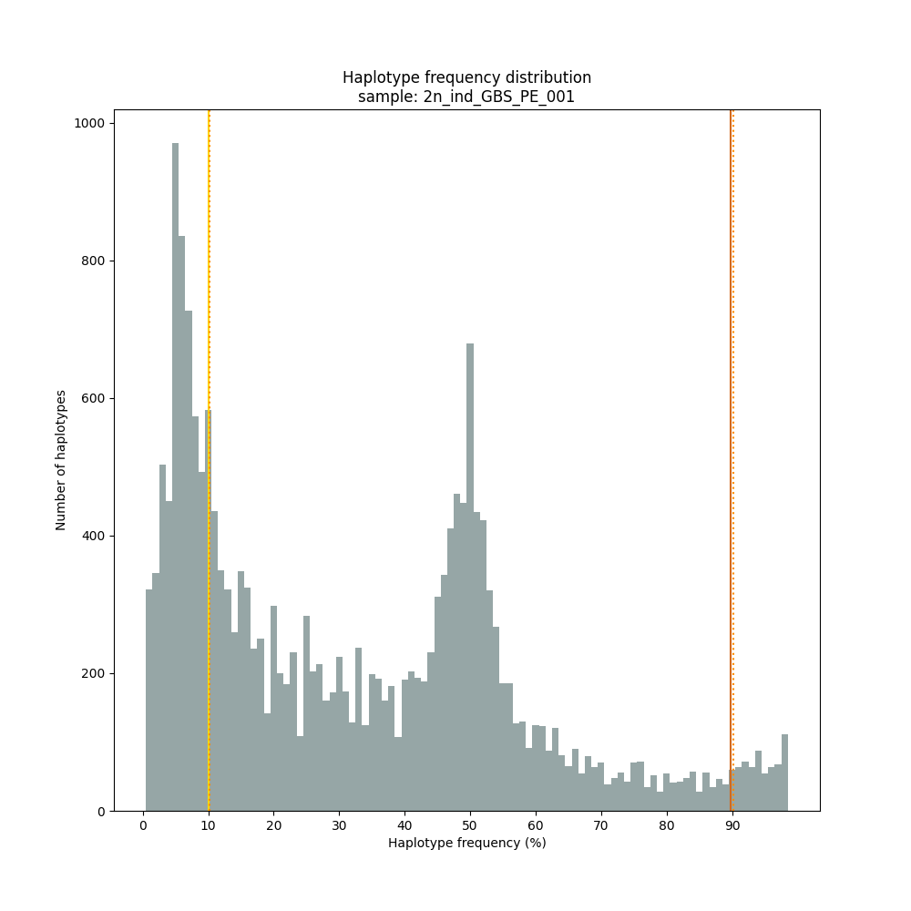
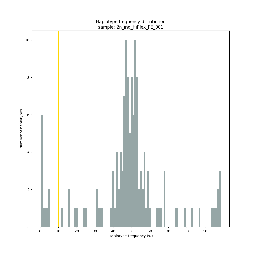
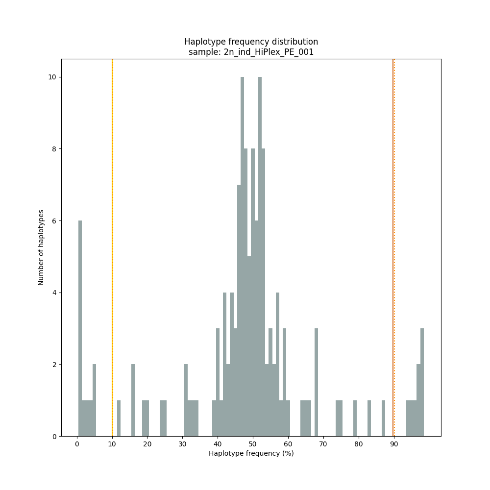
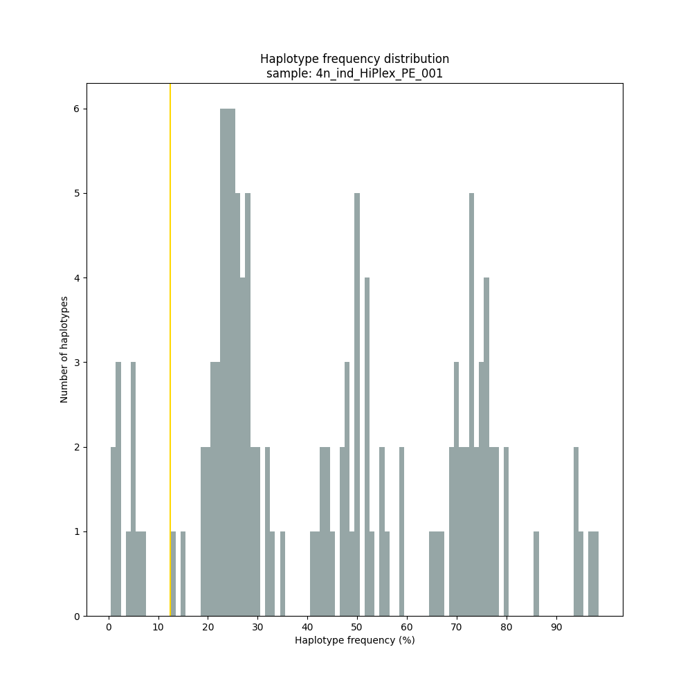
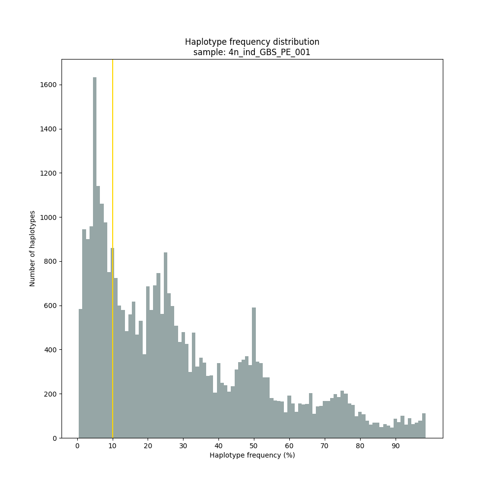
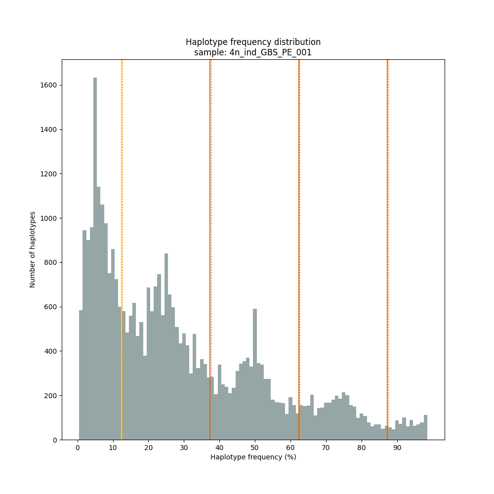
The different tabs below show the typical haplotype frequency distributions of diploid or tetraploid individuals for GBS or HiPlex data. Vertical lines in the haplotype frequency distributions show the thresholds by which haplotype frequency is transformed into discrete call classes. The commands to run SMAP haplotype-sites on these datatypes are shown below each graph.
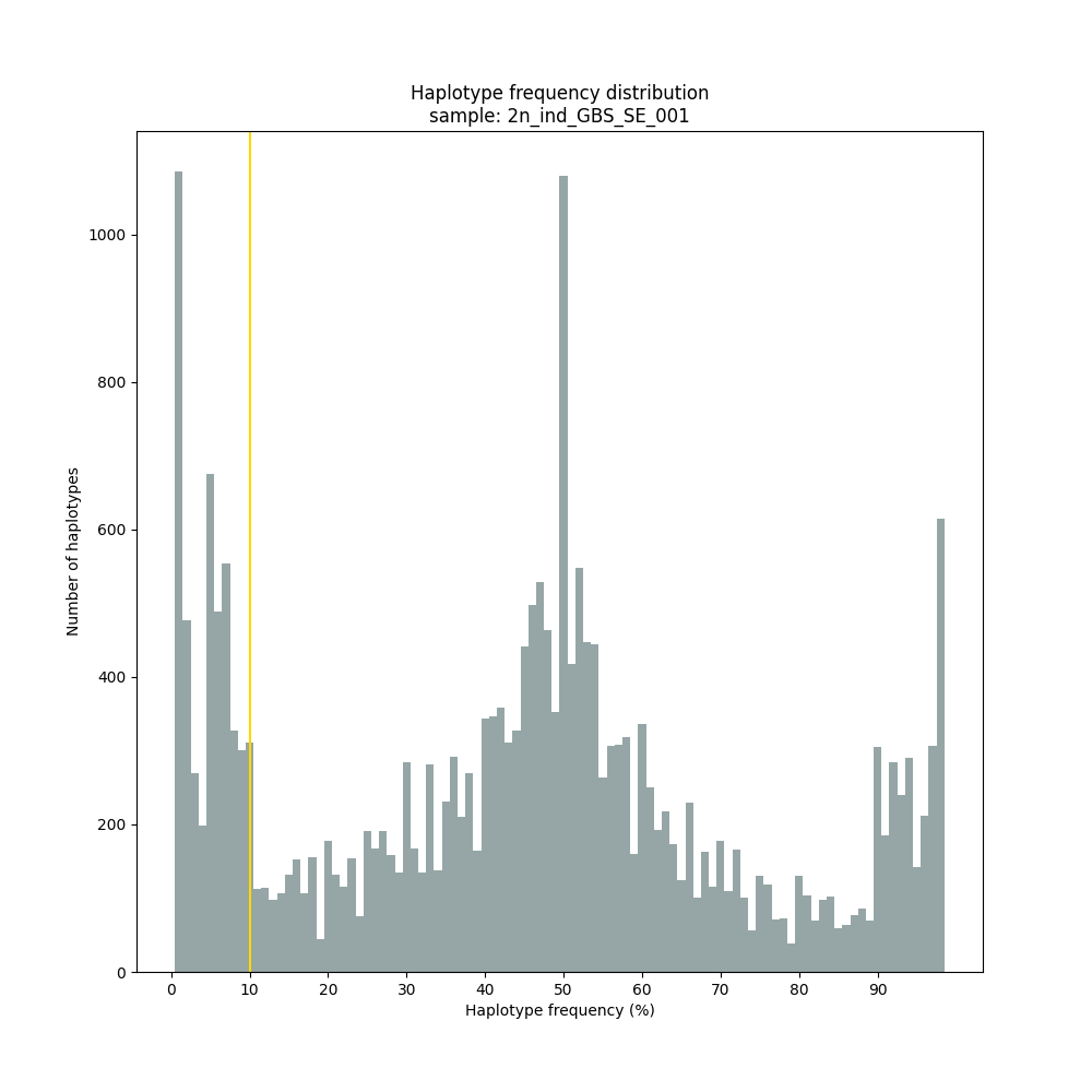
smap haplotype-sites /path/to/BAM/ /path/to/BED/ /path/to/VCF/ -mapping_orientation stranded -partial include --no_indels --min_read_count 10 -f 5 -p 8 --min_distinct_haplotypes 2 --plot_type png --plot all -o 2n_ind_GBS_SE_NI_DOMdiplo --discrete_calls dominant --frequency_interval_bounds 10
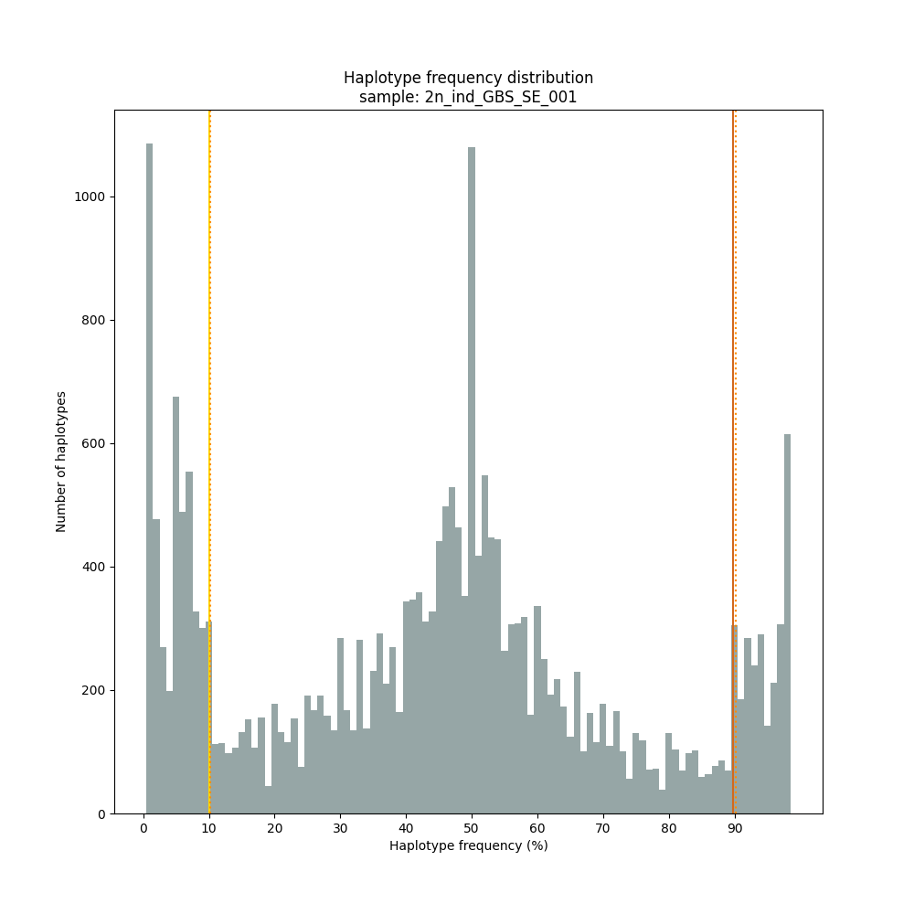
smap haplotype-sites /path/to/BAM/ /path/to/BED/ /path/to/VCF/ -mapping_orientation stranded -partial include --no_indels --min_read_count 10 -f 5 -p 8 --min_distinct_haplotypes 2 --plot_type png --plot all -o 2n_ind_GBS_SE_NI_DOSdiplo --discrete_calls dosage --frequency_interval_bounds 10 10 90 90 --dosage_filter 2
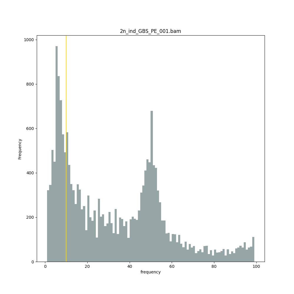
smap haplotype-sites /path/to/BAM/ /path/to/BED/ /path/to/VCF/ -mapping_orientation ignore -partial include --no_indels --min_read_count 10 -f 5 -p 8 --min_distinct_haplotypes 2 --plot_type png --plot all -o 2n_ind_GBS_PE_NI_DOMdiplo --discrete_calls dominant --frequency_interval_bounds 10
smap haplotype-sites /path/to/BAM/ /path/to/BED/ /path/to/VCF/ -mapping_orientation ignore -partial include --no_indels --min_read_count 10 -f 5 -p 8 --min_distinct_haplotypes 2 --plot_type png --plot all -o 2n_ind_GBS_PE_NI_DOSdiplo --discrete_calls dosage --frequency_interval_bounds 10 10 90 90 --dosage_filter 2
smap haplotype-sites /path/to/BAM/ /path/to/BED/ /path/to/VCF/ -mapping_orientation ignore -partial exclude --no_indels --min_read_count 10 -f 1 -p 8 --min_distinct_haplotypes 2 --plot_type png --plot all -o 2n_ind_HiPlex_NI_NP_DOMdiplo --discrete_calls dominant --frequency_interval_bounds 10
smap haplotype-sites /path/to/BAM/ /path/to/BED/ /path/to/VCF/ -mapping_orientation ignore -partial exclude --no_indels --min_read_count 10 -f 1 -p 8 --min_distinct_haplotypes 2 --plot_type png --plot all -o 2n_ind_HiPlex_NI_NP_DOSdiplo --discrete_calls dosage --frequency_interval_bounds 10 10 90 90 --dosage_filter 2
smap haplotype-sites /path/to/BAM/ /path/to/BED/ /path/to/VCF/ -mapping_orientation ignore -partial exclude --no_indels --discrete_calls dominant --frequency_interval_bounds 10 --min_read_count 10 -f 5 -p 8 --min_distinct_haplotypes 2 --plot_type png --plot all -o 4n_ind__NI_NP_DOMtetra
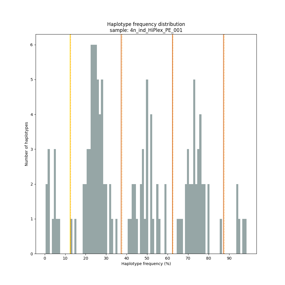
smap haplotype-sites /path/to/BAM/ /path/to/BED/ /path/to/VCF/ -mapping_orientation ignore -partial exclude --no_indels --discrete_calls dosage --frequency_interval_bounds 12.5 12.5 37.5 37.5 62.5 62.5 87.5 87.5 --dosage_filter 4 --min_read_count 10 -f 5 -p 8 --min_distinct_haplotypes 2 --plot_type png --plot all -o 4n_ind__NI_NP_DOStetra
smap haplotype-sites /path/to/BAM/ /path/to/BED/ /path/to/VCF/ -mapping_orientation ignore -partial include --no_indels --discrete_calls dominant --frequency_interval_bounds 10 --min_read_count 10 -f 5 -p 8 --min_distinct_haplotypes 2 --plot_type png --plot all -o 4n_ind_GBS_PE_NI_DOMtetra
smap haplotype-sites /path/to/BAM/ /path/to/BED/ /path/to/VCF/ -mapping_orientation ignore -partial include --no_indels --discrete_calls dosage --frequency_interval_bounds 12.5 12.5 37.5 37.5 62.5 62.5 87.5 87.5 --dosage_filter 4 --min_read_count 10 -f 5 -p 8 --min_distinct_haplotypes 2 --plot_type png --plot all -o 4n_ind_GBS_PE_NI_DOStetra
Step 5: Transforming haplotype frequencies to discrete calls in individuals
procedure
If individual genotypes are analysed in, the final step is to transform observed haplotype frequencies per individual back to discrete haplotype calls using --discrete_calls. SMAP haplotype-sites uses simple, user-defined haplotype frequency thresholds to define discrete genotypic classes. The multi-allelic nature of haplotype calling is retained, and the final genotype call table lists the absence/presence (0/1) or dosage (0/1/2 diploids; 0/1/2/3/4 tetraploids) of each haplotype per individual.
Next, the total count of discrete haplotypes per locus per sample is calculated and output as a table. See examples below.
Alternatively, haplotype read depth data generated with SMAP haplotype-sites may be used as input for genotype calling in individuals using statistical methods, for instance Clark et al. 2019.
Haplotype count tables
If SMAP haplotype-sites is run using --discrete_calls the analysis continues by creating discrete haplotype calls per individual sample. For each sample and for each locus, haplotype frequencies are transformed to discrete calls using simple user-defined frequency thresholds based on the observed haplotype frequency spectrum.
Next, the total count of discrete haplotypes per locus per sample is calculated and output as table. See examples below.
Per diploid sample, loci with a total haplotype count different from a set value (--dosage_filter) are removed (set to `NaN´ ). The recommended value for this filter is 2 for diploids and 4 for tetraploids. The haplotype frequency is then calculated across the set of samples (count per haplotype/total haplotype count per locus * 100%). This measure identifies the haplotypes that are supported by sufficient read depth in individual genotypes, but rare across the sample set (e.g. population).
Locus |
2n_ind_GBS-SE_001.bam |
2n_ind_GBS-SE_002.bam |
2n_ind_GBS-SE_003.bam |
2n_ind_GBS-SE_004.bam |
2n_ind_GBS-SE_005.bam |
2n_ind_GBS-SE_006.bam |
2n_ind_GBS-SE_007.bam |
2n_ind_GBS-SE_008.bam |
|---|---|---|---|---|---|---|---|---|
Chrom_1:15617-15711/+ |
2 |
2 |
2 |
2 |
2 |
2 |
2 |
1 |
Chrom_1:15712-15798/- |
2 |
2 |
2 |
2 |
2 |
2 |
2 |
1 |
In -f 1 filtering, haplotypes with a frequency lower than 1% across all samples are removed. This is done in order to remove noise. It is recommended to try out different values and decide which value suits your data best.
Locus |
2n_ind_GBS-SE_001.bam |
2n_ind_GBS-SE_002.bam |
2n_ind_GBS-SE_003.bam |
2n_ind_GBS-SE_004.bam |
2n_ind_GBS-SE_005.bam |
2n_ind_GBS-SE_006.bam |
2n_ind_GBS-SE_007.bam |
2n_ind_GBS-SE_008.bam |
|---|---|---|---|---|---|---|---|---|
Chrom_1:15617-15711/+ |
2 |
2 |
2 |
2 |
2 |
2 |
2 |
1 |
Chrom_1:15712-15798/- |
2 |
2 |
2 |
2 |
2 |
2 |
2 |
1 |
In -f 5 filtering, haplotypes with a frequency lower than 5% across all samples are removed. This is done in order to remove noise. It is recommended to try out different values and decide which value suits your data best.
Locus |
2n_ind_GBS-SE_001.bam |
2n_ind_GBS-SE_002.bam |
2n_ind_GBS-SE_003.bam |
2n_ind_GBS-SE_004.bam |
2n_ind_GBS-SE_005.bam |
2n_ind_GBS-SE_006.bam |
2n_ind_GBS-SE_007.bam |
2n_ind_GBS-SE_008.bam |
|---|---|---|---|---|---|---|---|---|
Chrom_1:15617-15711/+ |
2 |
2 |
2 |
2 |
2 |
2 |
2 |
1 |
Chrom_1:15712-15798/- |
2 |
2 |
2 |
2 |
2 |
2 |
2 |
2 |
Haplotype call tables
Haplotype allele frequencies are calculated as the number of observations of a haplotype divided by the total number of haplotype observations (ploidy (or --dosage_filter value) x number of samples with observations) on that locus. In -f 0 filtering, all haplotypes are retained. It is recommended to try out different values and decide which value suits your data best.
Locus |
haplotype |
2n_ind_GBS-SE_001.bam |
2n_ind_GBS-SE_002.bam |
2n_ind_GBS-SE_003.bam |
2n_ind_GBS-SE_004.bam |
2n_ind_GBS-SE_005.bam |
2n_ind_GBS-SE_006.bam |
2n_ind_GBS-SE_007.bam |
2n_ind_GBS-SE_008.bam |
HF |
Total_obs |
|---|---|---|---|---|---|---|---|---|---|---|---|
Chrom_1:15618-15711_+ |
.01000000000 |
1 |
0 |
0 |
0 |
0 |
0 |
2 |
NA |
21.43 |
14 |
Chrom_1:15618-15711_+ |
.01000100000 |
0 |
1 |
0 |
0 |
0 |
0 |
0 |
NA |
7.14 |
14 |
Chrom_1:15618-15711_+ |
.01001010110 |
0 |
0 |
0 |
1 |
0 |
0 |
0 |
NA |
7.14 |
14 |
Chrom_1:15618-15711_+ |
.01010000000 |
0 |
0 |
0 |
0 |
1 |
0 |
0 |
NA |
7.14 |
14 |
Chrom_1:15618-15711_+ |
.01100000000 |
0 |
0 |
1 |
0 |
0 |
0 |
0 |
NA |
7.14 |
14 |
Chrom_1:15618-15711_+ |
000000000… |
1 |
1 |
1 |
1 |
1 |
2 |
0 |
NA |
50.00 |
14 |
Chrom_1:15713-15798_- |
00000000 |
1 |
1 |
1 |
1 |
1 |
2 |
0 |
NA |
50.00 |
14 |
Chrom_1:15713-15798_- |
010010.. |
0 |
0 |
0 |
1 |
0 |
0 |
0 |
NA |
7.14 |
14 |
Chrom_1:15713-15798_- |
01111010 |
1 |
1 |
1 |
0 |
1 |
0 |
2 |
NA |
42.86 |
14 |
Haplotype allele frequencies are calculated as the number of observations of a haplotype divided by the total number of haplotype observations (ploidy (or --dosage_filter value) x number of samples with observations) on that locus. In -f 1 filtering, haplotypes with a frequency lower than 1% across all samples are removed. This is done in order to remove noise. It is recommended to try out different values and decide which value suits your data best.
Locus |
haplotype |
2n_ind_GBS-SE_001.bam |
2n_ind_GBS-SE_002.bam |
2n_ind_GBS-SE_003.bam |
2n_ind_GBS-SE_004.bam |
2n_ind_GBS-SE_005.bam |
2n_ind_GBS-SE_006.bam |
2n_ind_GBS-SE_007.bam |
2n_ind_GBS-SE_008.bam |
HF |
Total_obs |
|---|---|---|---|---|---|---|---|---|---|---|---|
Chrom_1:15618-15711_+ |
.01000000000 |
1 |
0 |
0 |
0 |
0 |
0 |
2 |
NA |
21.43 |
14 |
Chrom_1:15618-15711_+ |
.01000100000 |
0 |
1 |
0 |
0 |
0 |
0 |
0 |
NA |
7.14 |
14 |
Chrom_1:15618-15711_+ |
.01001010110 |
0 |
0 |
0 |
1 |
0 |
0 |
0 |
NA |
7.14 |
14 |
Chrom_1:15618-15711_+ |
.01010000000 |
0 |
0 |
0 |
0 |
1 |
0 |
0 |
NA |
7.14 |
14 |
Chrom_1:15618-15711_+ |
.01100000000 |
0 |
0 |
1 |
0 |
0 |
0 |
0 |
NA |
7.14 |
14 |
Chrom_1:15618-15711_+ |
000000000… |
1 |
1 |
1 |
1 |
1 |
2 |
0 |
NA |
50.00 |
14 |
Chrom_1:15713-15798_- |
00000000 |
1 |
1 |
1 |
1 |
1 |
2 |
0 |
NA |
50.00 |
14 |
Chrom_1:15713-15798_- |
010010.. |
0 |
0 |
0 |
1 |
0 |
0 |
0 |
NA |
7.14 |
14 |
Chrom_1:15713-15798_- |
01111010 |
1 |
1 |
1 |
0 |
1 |
0 |
2 |
NA |
42.86 |
14 |
Haplotype allele frequencies are calculated as the number of observations of a haplotype divided by the total number of haplotype observations (ploidy (or --dosage_filter value) x number of samples with observations) on that locus. In -f 5 filtering, haplotypes with a frequency lower than 5% across all samples are removed. This is done in order to remove noise. It is recommended to try out different values and decide which value suits your data best.
Locus |
haplotype |
2n_ind_GBS-SE_001.bam |
2n_ind_GBS-SE_002.bam |
2n_ind_GBS-SE_003.bam |
2n_ind_GBS-SE_004.bam |
2n_ind_GBS-SE_005.bam |
2n_ind_GBS-SE_006.bam |
2n_ind_GBS-SE_007.bam |
2n_ind_GBS-SE_008.bam |
HF |
Total_obs |
|---|---|---|---|---|---|---|---|---|---|---|---|
Chrom_1:15618-15711_+ |
.01000000000 |
1 |
0 |
0 |
0 |
0 |
0 |
2 |
NA |
21.43 |
14 |
Chrom_1:15618-15711_+ |
.01000100000 |
0 |
1 |
0 |
0 |
0 |
0 |
0 |
NA |
7.14 |
14 |
Chrom_1:15618-15711_+ |
.01001010110 |
0 |
0 |
0 |
1 |
0 |
0 |
0 |
NA |
7.14 |
14 |
Chrom_1:15618-15711_+ |
.01010000000 |
0 |
0 |
0 |
0 |
1 |
0 |
0 |
NA |
7.14 |
14 |
Chrom_1:15618-15711_+ |
.01100000000 |
0 |
0 |
1 |
0 |
0 |
0 |
0 |
NA |
7.14 |
14 |
Chrom_1:15618-15711_+ |
000000000… |
1 |
1 |
1 |
1 |
1 |
2 |
0 |
NA |
50.00 |
14 |
Chrom_1:15713-15798_- |
00000000 |
1 |
1 |
1 |
1 |
1 |
2 |
0 |
0 |
43.75 |
16 |
Chrom_1:15713-15798_- |
010010.. |
0 |
0 |
0 |
1 |
0 |
0 |
0 |
0 |
6.25 |
16 |
Chrom_1:15713-15798_- |
01111010 |
1 |
1 |
1 |
0 |
1 |
0 |
2 |
2 |
50.00 |
16 |
Step 6: Filtering for high quality dosage calls in individuals
procedure
If individual genotypes are analysed in mode for dosage calls, the final step is to check if the total number of alleles equals that expected for the ploidy of the individual (2 in diploids, and 4 in tetraploids). All locus/sample combinations that do not show the expected number of haplotypes are removed from the genotyping table. In addition, two scores are calculated per sample: the completeness of observations across all tested loci, and the proportion of loci with correct genotype call, across all observed loci for that sample. two scores are calculated per locus: the completeness of observations across all tested sample, and the proportion of samples with correct genotype call, across all observed samples for that locus. A list is created with loci that display a minimum correctness across all observations, and only good quality loci are reported in the final genotype table. SMAP haplotype-sites uses simple, user-defined correctness filters to select high quality genotyping data, and the final genotype call table lists the dosage (0/1/2 diploids; 0/1/2/3/4 tetraploids) of each haplotype per individual.
Output
Tabular output
By default, SMAP haplotype-sites will return two .tsv files.
Read_counts_cx_fx_mx.tsv (with x the value per option used in the analysis) contains the read counts (-c) and haplotype frequency (-f) filtered and/or masked (-m) read counts per haplotype per locus as defined in the BED file from SMAP delineate.
This is the file structure:
Locus
Haplotypes
Sample1
Sample2
Sample..
Chr1:100-200
00010
0
13
34
Chr1:100-200
01000
19
90
28
Chr1:100-200
00110
60
0
23
Chr1:450-600
0010
70
63
87
Chr1:450-600
0110
108
22
134
Haplotype_frequencies_cx_fx_mx.tsv contains the relative frequency per haplotype per locus in sample (based on the corresponding count table: Read_counts_cx_fx_mx.tsv). The transformation to relative frequency per locus-sample combination inherently normalizes for differences in total number of mapped reads across samples, and differences in amplification efficiency across loci. This is the file structure:
Locus
Haplotypes
Sample1
Sample2
Sample..
Chr1:100-200
00010
0
0.13
0.40
Chr1:100-200
01000
0.24
0.87
0.33
Chr1:100-200
00110
0.76
0
0.27
Chr1:450-600
0010
0.39
0.74
0.39
Chr1:450-600
0110
0.61
0.26
0.61
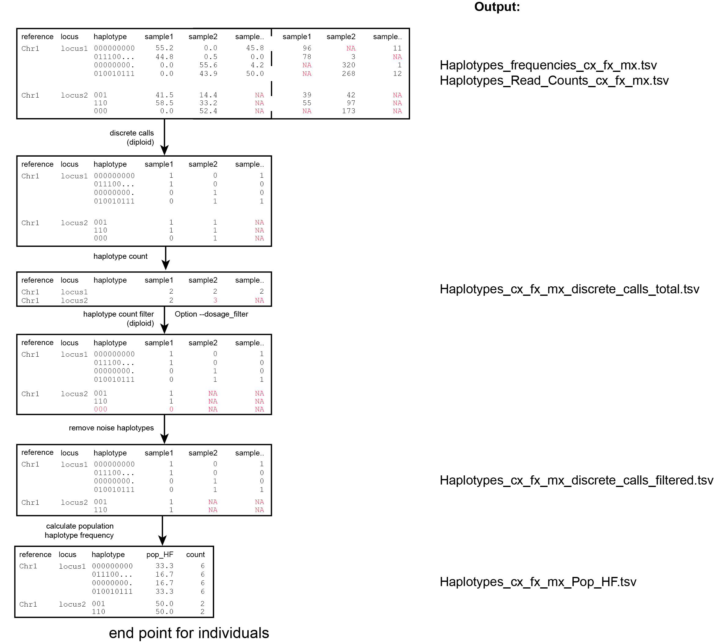
For individuals, if the option --discrete_calls is used, the program will return three additional .tsv files. Their content and order of creation is shown in the image above.
The first file is called haplotypes_cx_fx_mx_discrete_calls._total.tsv and this file contains the total dosage calls, obtained after transforming haplotype frequencies into discrete calls, using the defined--frequency_interval_bounds. The total sum of discrete dosage calls is expected to be 2 in diploids and 4 in tetraploids.
Locus
Sample1
Sample2
Sample..
Chr1:100-200
2
2
3
Chr1:450-600
2
2
2
The second file is haplotypes_cx_fx_mx-discrete_calls_filtered.tsv, which lists the discrete calls per locus per sample after--dosage_filterhas removed loci per sample with an unexpected number of haplotype calls (as listed in haplotypes_cx_fx_mx_discrete_calls_total.tsv). The expected number of calls is set with option-z[use 2 for diploids, 4 for tetraploids].
Locus
Haplotypes
Sample1
Sample2
Sample..
Chr1:100-200
00010
0
1
NA
Chr1:100-200
01000
1
1
NA
Chr1:100-200
00110
1
0
NA
Chr1:450-600
0010
1
1
1
Chr1:450-600
0110
1
1
1
The third file, haplotypes_cx_fx_mx_Pop_HF.tsv, lists the population haplotype frequencies (over all individual samples) based on the total number of discrete haplotype calls relative to the total number of calls per locus.
Locus
Haplotypes
Pop_HF
count
Chr1:100-200
00010
25.0
4
Chr1:100-200
01000
50.0
4
Chr1:100-200
00110
25.0
4
Chr1:450-600
0010
50.0
6
Chr1:450-600
0110
50.0
6
For individuals, if the option--locus_correctnessis used in combination with--discrete_callsand--frequency_interval_bounds, the programm will create a new .bed file haplotypes_cx_fx_mx_correctness_loci.bed (loci filtered from the input .bed file) containing only the loci that were correctly dosage called (-z) in at least the defined percentage of samples. See above.
Reference
Start
End
HiPlex_locus_name
Mean_read_depth
Strand
SMAPs
Completeness
nr_SMAPs
Name
Chr1
100
200
Chr1_100-200
.
+
100,199
.
2
HiPlex_Set1
Chr1
450
600
Chr1_450-600
.
+
450,599
.
2
HiPlex_Set1
Graphical output
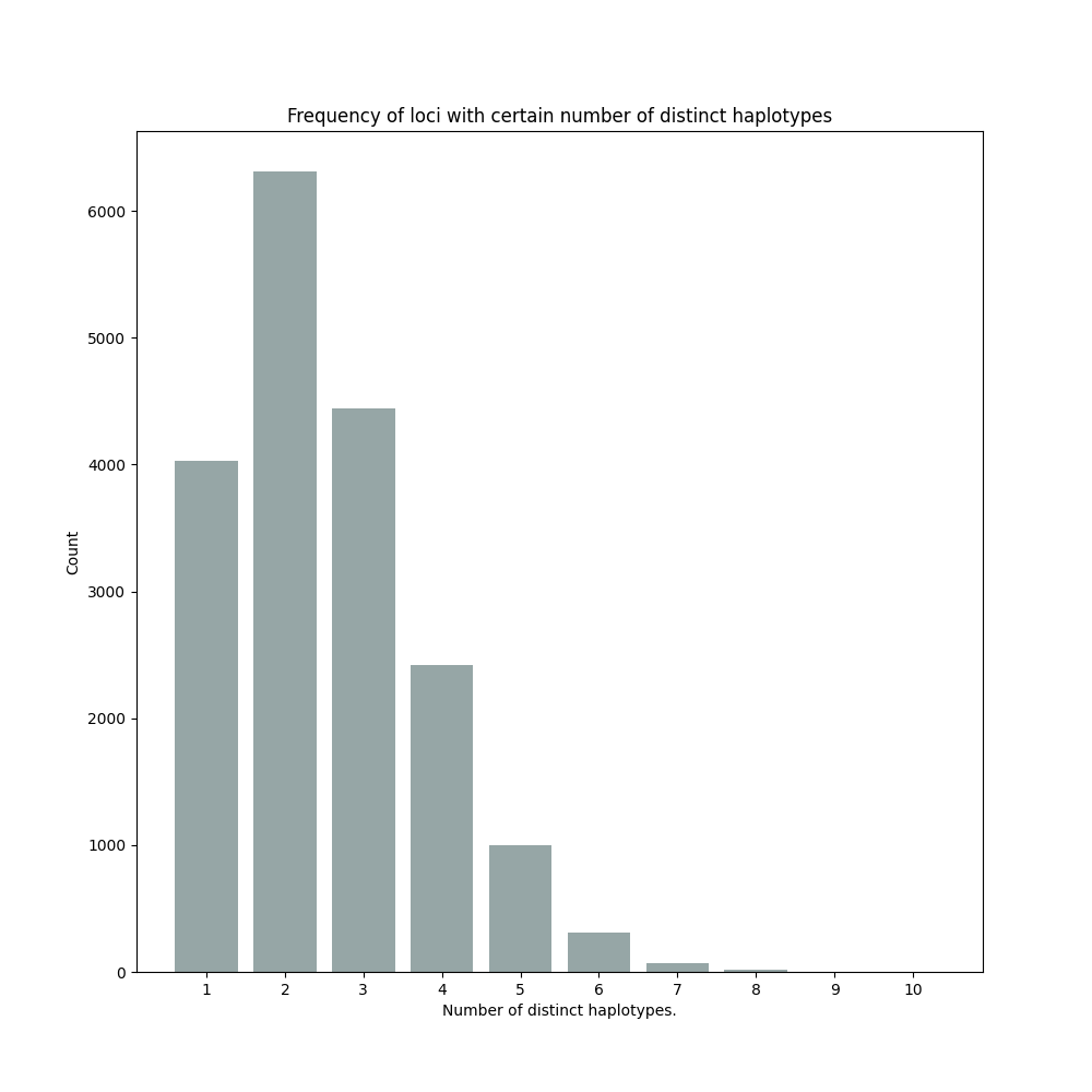
By default, SMAP haplotype-sites will generate graphical output summarizing haplotype diversity. haplotype_diversity_across_sampleset.png shows a histogram of the number of distinct haplotypes per locus across all samples.
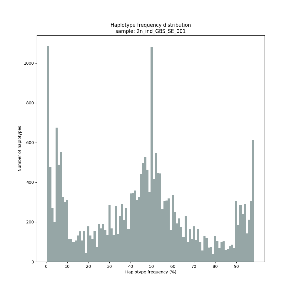
Graphical output of the haplotype frequency distribution for each individual sample can be switched on using the option --plot all. sample_haplotype_frequency_distribution.png shows the haplotype frequency distribution across all loci detected per sample. It is the graphical representation of each sample-specific column in haplotypes_cx_fx_mx.tsv. Using the option --discrete_calls, this plot will also show the defined discrete calling boundaries.
After discrete genotype calling with option
--discrete_calls, SMAP haplotype-sites will evaluate the observed sum of discrete dosage calls per locus per sample versus the expected value per locus (set with option-z, recommended use: 2 for diploid, 4 for tetraploid).
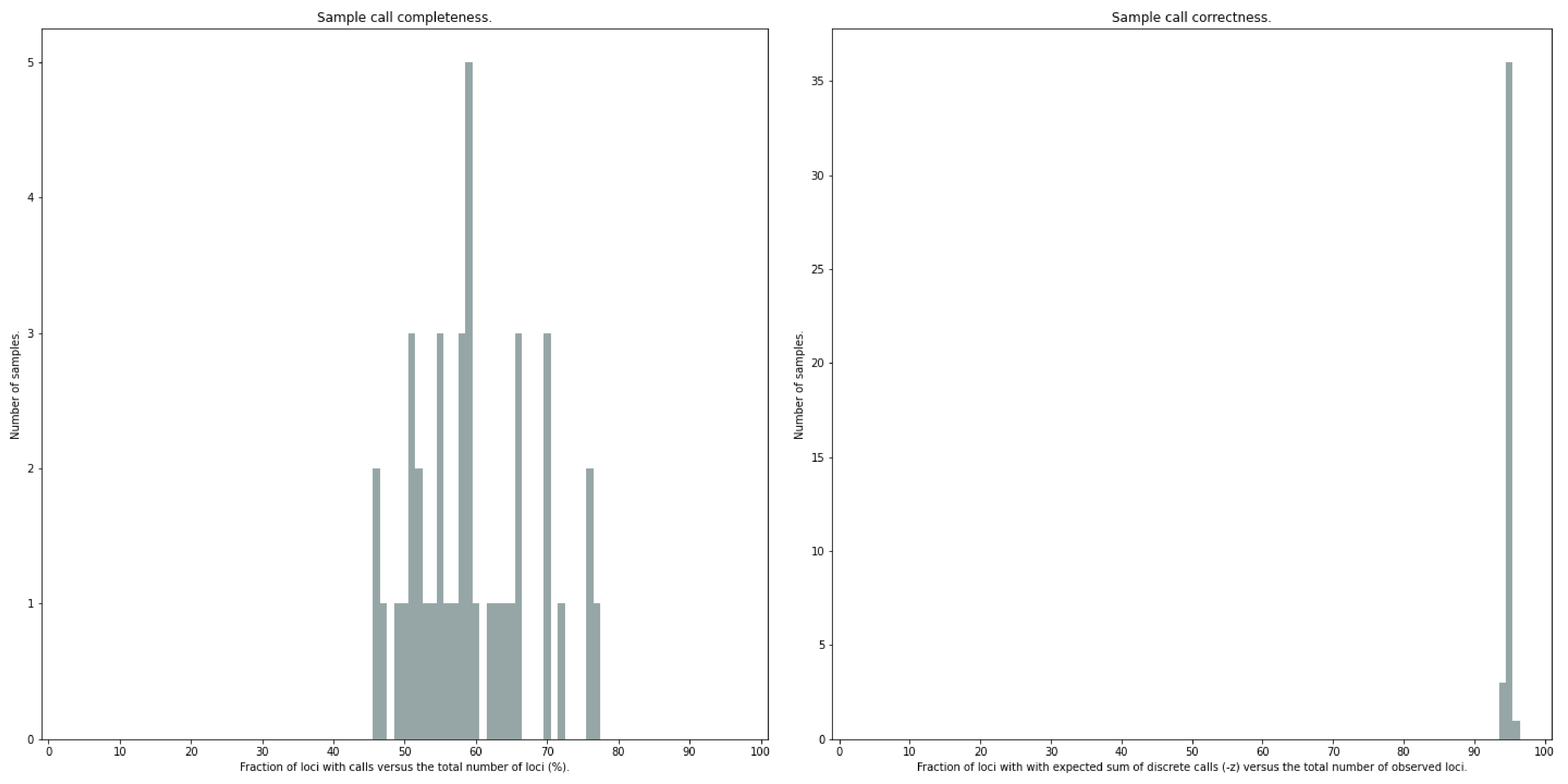
The quality of genotype calls per sample is calculated in two ways: the fraction of loci with calls in that sample versus the total number of loci across all samples (sample_call_completeness); the fraction of loci with expected sum of discrete dosage calls (-z) versus the total number of observed loci in that sample (sample_call_correctness). These scores are calculated separately per sample, and SMAP haplotype-sites plots the distribution of those scores across the sample set (sampleset_call_completeness; sampleset_call_correctness).
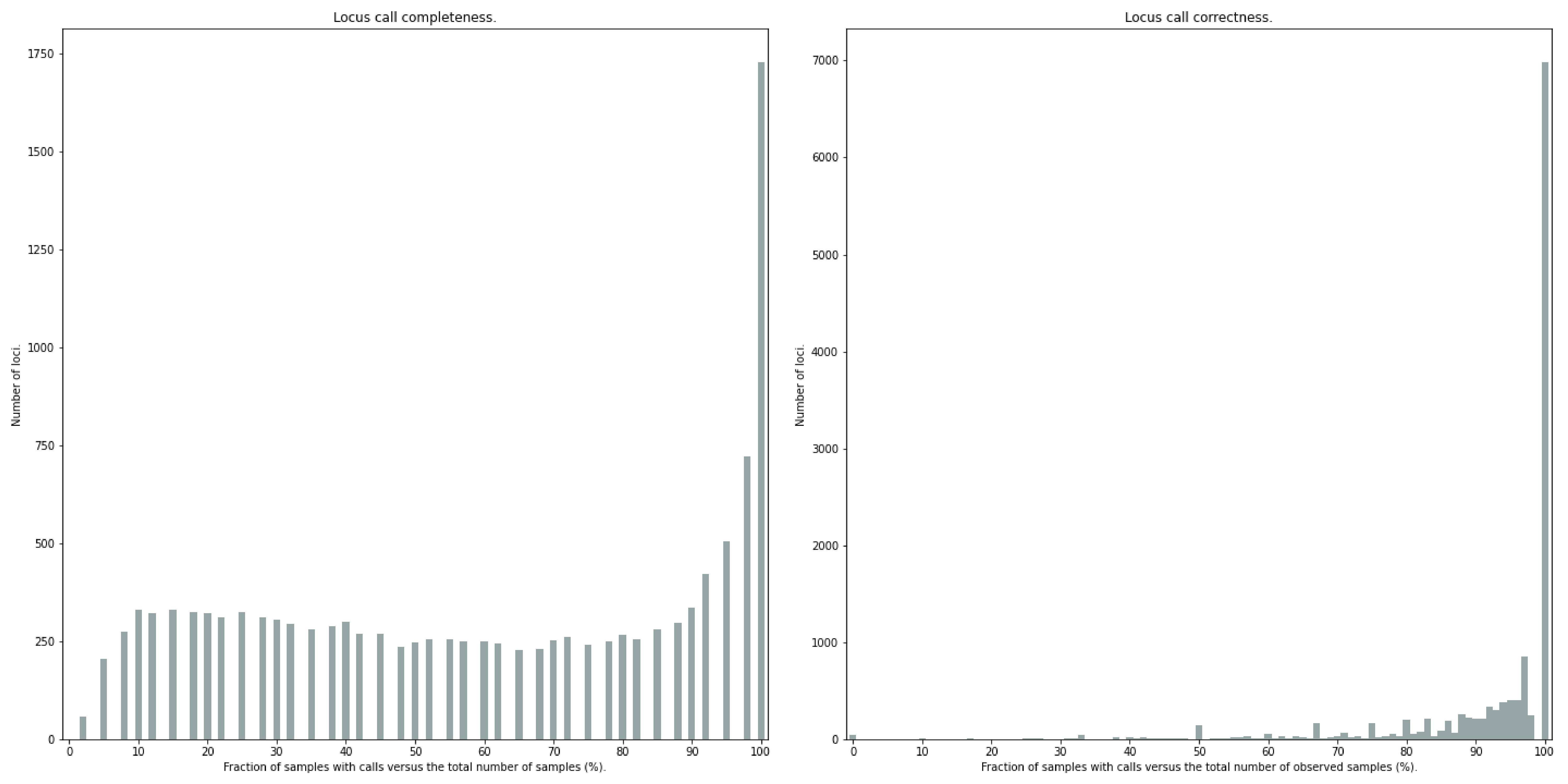
Similarly, the quality of genotype calls per locus is calculated in two ways: the fraction of samples with calls for that locus versus the total number of samples (locus_call_completeness); the fraction of samples with expected sum of discrete dosage calls (-z) versus the total number of observed samples for that locus (locus_call_correctness). These scores are calculated separately per locus, and SMAP haplotype-sites plots the distribution of those scores across the locus set (locusset_call_completeness; locusset_call_correctness).
Both graphs and the corresponding tables (one for samples and one for loci) can be evaluated to identify poorly performing samples and/or loci. We recommend to eliminate these from further analysis by removing BAM files from the run directory and/or loci from the SMAP delineate BED file with SMAPs, and iterate through rounds of data analysis combined with sample and locus quality control.
Summary of Commands
-mapping_orientation stranded or -mapping_orientation ignorealignments_dir ############# (str) ### Path to the directory containing BAM and BAI files. All BAM files should be in the same directory. Positional mandatory argument, should be the first argument after smap haplotype-sites [no default].bed ##################### (str) ### Path to the BED file containing sites for which haplotypes will be reconstructed. For GBS experiments, the BED file should be generated using SMAP delineate. For HiPlex data, a BED6 file can be provided, with the 4th and 5th column being blank and the chromosome name, locus start position site, locus end position site and strand information populating the first, second, third and sixth column respectively. Positional mandatory argument, should be the second argument after smap haplotype-sites.vcf ##################### (str) ### Path to the VCF file (in VCFv4.1 format) containing variant positions. It should contain at least the first 9 columns listing the SNP positions, sample-specific genotype calls across the sampleset are not required. Positional mandatory argument, should be the third argument after smap haplotype-sites.-p, --processes ########### (int) ### Number of parallel processes [1].--plot ######################### Select which plots are to be generated. Choosing “nothing” disables plot generation. Passing “summary” only generates graphs with information for all samples while “all” will also enable generate per-sample plots [default “summary”].-t, --plot_type ################## Use this option to choose plot format, choices are png and pdf [png].-o, --out ############### (str) ### Basename of the output file without extension [SMAP_haplotype_sites].-u, --undefined_representation ####### Value to use for non-existing or masked data [NaN].-h, --help ##################### Show the full list of options. Disregards all other parameters.-v, --version ################### Show the version. Disregards all other parameters.--debug ######################## Enable verbose logging.-q, --min_mapping_quality #### (int) ### Minimum .bam mapping quality to retain reads for analysis [30].--no_indels ##################### Use this option if you want to exclude haplotypes that contain an InDel at the given SNP/SMAP positions. These reads are also ignored to evaluate the minimum read count [default off; indels are included in output].-j, --min_distinct_haplotypes # (int) ### Minimum number of distinct haplotypes per locus across all samples. Loci that do not fit this criterium are removed from the final output [0].-k, --max_distinct_haplotypes # (int) ### Maximum number of distinct haplotypes per locus across all samples. Loci that do not fit this criterium are removed from the final output [inf].-c, --min_read_count ####### (int) ### Minimum total number of reads per locus per sample [0].-d, --max_read_count ####### (int) ### Maximum number of reads per locus per sample, read count is calculated after filtering out the low frequency haplotypes (-f) [inf].-f, --min_haplotype_frequency # (float) ## Set minimum haplotype frequency (in %) to retain the haplotype in the genotyping matrix. Haplotypes above this threshold in at least one of the samples are retained. Haplotypes that never reach this threshold in any of the samples are removed [0].-m, --mask_frequency ####### (float) ## Mask haplotype frequency values below this threshold for individual samples to remove noise from the final output. Haplotype frequency values below this threshold are set to -u. Haplotypes are not removed based on this value, use --min_haplotype_frequency for this purpose instead.This option is primarily supported for diploids and tetraploids. Users can define their own custom frequency bounds for species with a higher ploidy, but this requires optimization based on the observed haplotype frequency distributions.
-e, --discrete_calls ### (str) ### Set to “dominant” to transform haplotype frequency values into presence(1)/absence(0) calls per allele, or “dosage” to indicate the allele copy number.
-i, --frequency_interval_bounds ## Frequency interval bounds for classifying the read frequencies into discrete calls. Custom thresholds can be defined by passing one or more space-separated integers which represent relative frequencies in percentage. For dominant calling, one value should be specified. For dosage calling, an even total number of four or more thresholds should be specified. The usage of defaults can be enabled by passing either “diploid” or “tetraploid”. The default value for dominant calling (see discrete_calls argument) is 10, regardless whether or not “diploid” or “tetraploid” is used. For dosage calling, the default for diploids is “10 10 90 90” and for tetraploids “12.5 12.5 37.5 37.5 62.5 62.5 87.5 87.5”
-z, --dosage_filter ### (int) ### Mask dosage calls in the loci for which the total allele count for a given locus at a given sample differs from the defined value. For example, in diploid organisms the total allele copy number must be 2, and in tetraploids the total allele copy number must be 4. (default no filtering).
--locus_correctness ######## (int) ### Threshold value: % of samples with locus correctness. Create a new BED file defining only the loci that were correctly dosage called (-z) in at least the defined percentage of samples (default no filtering).
--frequency_interval_bounds in practical examples and additional information on the dosage filter can be found in the section recommendations.