Design a CRISPR/Cas experiment with gRNA and HiPlex panels (potato)
Activate your virtual environment
source .venv/bin/activate
Create the reference sequences
Define the path to the download directory:
download_dir=$/PATH/TO/DOWNLOAD_DIR/
Or, create a new download dir:
cd ../
mkdir download
cd download
download_dir=$(pwd)
Download genomes and gene annotation data:
cd $download_dir
mkdir originals
cd originals
wget https://ftp.psb.ugent.be/pub/plaza/plaza_public_dicots_05/GeneFamilies/genefamily_data.HOMFAM.csv.gz
wget https://ftp.psb.ugent.be/pub/plaza/plaza_public_dicots_05/GeneFamilies/genefamily_data.ORTHOFAM.csv.gz
wget https://ftp.psb.ugent.be/pub/plaza/plaza_public_dicots_05/Genomes/stu.fasta.gz
wget https://ftp.psb.ugent.be/pub/plaza/plaza_public_dicots_05/GFF/stu/annotation.selected_transcript.all_features.stu.gff3.gz
wget https://ftp.psb.ugent.be/pub/plaza/plaza_public_dicots_05/GFF/stu/annotation.selected_transcript.exon_features.stu.gff3.gz
wget https://ftp.psb.ugent.be/pub/plaza/plaza_public_dicots_05/Annotation/annotation.selected_transcript.stu.csv.gz
wget https://ftp.psb.ugent.be/pub/plaza/plaza_public_dicots_05/IdConversion/id_conversion.stu.csv.gz
wget https://ftp.psb.ugent.be/pub/plaza/plaza_public_dicots_05/Descriptions/gene_description.stu.csv.gz
wget https://ftp.psb.ugent.be/pub/plaza/plaza_public_dicots_05/GO/go.stu.csv.gz
wget https://ftp.psb.ugent.be/pub/plaza/plaza_public_dicots_05/InterPro/interpro.stu.csv.gz
wget https://ftp.psb.ugent.be/pub/plaza/plaza_public_dicots_05/MapMan/mapman.stu.csv.gz
wget https://ftp.psb.ugent.be/pub/plaza/plaza_public_dicots_05/Fasta/proteome.selected_transcript.stu.fasta.gz
wget https://ftp.psb.ugent.be/pub/plaza/plaza_public_dicots_05/Fasta/transcripts.selected_transcript.stu.fasta.gz
wget https://ftp.psb.ugent.be/pub/plaza/plaza_public_dicots_05/Fasta/cds.selected_transcript.stu.fasta.gz
Unzip and change some formats for SMAP target-selection and place in SMAP_reference directory:
mkdir ../../SMAP_reference
zcat genefamily_data.HOMFAM.csv.gz | grep -v "#" > ../../SMAP_reference/genefamily_data.HOMFAM.csv
zcat genefamily_data.ORTHOFAM.csv.gz | grep -v "#" > ../../SMAP_reference/genefamily_data.ORTHOFAM.csv
zcat stu.fasta.gz > ../../SMAP_reference/stu.fasta
zcat annotation.selected_transcript.stu.csv.gz > ../../SMAP_reference/annotation.selected_transcript.stu.csv
zcat annotation.selected_transcript.all_features.stu.gff3.gz > ../../SMAP_reference/annotation.selected_transcript.all_features.stu.gff3
These files may be used later:
zcat annotation.selected_transcript.all_features.stu.gff3.gz > ../../SMAP_reference/annotation.selected_transcript.all_features.stu.gff3
zcat annotation.selected_transcript.exon_features.stu.gff3.gz > ../../SMAP_reference/annotation.selected_transcript.exon_features.stu.gff3
zcat gene_description.stu.csv.gz > ../../SMAP_reference/gene_description.stu.csv
zcat go.stu.csv.gz > ../../SMAP_reference/go.stu.csv
zcat interpro.stu.csv.gz > ../../SMAP_reference/interpro.stu.csv
zcat mapman.stu.csv.gz > ../../SMAP_reference/mapman.stu.csv
zcat proteome.selected_transcript.stu.fasta.gz > ../../SMAP_reference/proteome.selected_transcript.stu.fasta
zcat transcripts.selected_transcript.stu.fasta.gz > ../../SMAP_reference/transcripts.selected_transcript.stu.fasta
zcat cds.selected_transcript.stu.fasta.gz > ../../SMAP_reference/cds.selected_transcript.stu.fasta
Create short_list of homology groups in the SMAP_reference directory:
cd ../../SMAP_reference
echo "HOM05D000431" > shortlist_HOM.tsv
Add as many different homology groups as you like:
echo "HOM05D000432" >> shortlist_HOM.tsv
Create fasta reference files per homology group with SMAP target-selection (use ./ notation to indicate the path to this directory, otherwise the script tries to write files to the root of the system, where is has no write access rights).:
smap target-selection ./annotation.selected_transcript.all_features.stu.gff3 ./stu.fasta ./genefamily_data.HOMFAM.csv stu --region 1000 --hom_groups ./shortlist_HOM.tsv
Troubleshooting
In some cases the GFF file contains formatting errors in a subset of the genes, that cause problems when processing the GFF file with gffutils. In this case a quick workaround is to try to extract the gff features from the candidate genes only, and use that GFF file as input for SMAP target-selection.
Create a short_list of candidate genes for the list of selected homology groups of the species of interest (the corresponding gene_IDs are listed in the third column of the file genefamily_data.HOMFAM.csv)
grep -f shortlist_HOM.tsv ./genefamily_data.HOMFAM.csv | grep "stu" | cut -f3 > genelist_HOM05D000431_HOM05D000432.txt
Extract the gff features for each of the candidate genes from the original GFF file
grep -f genelist_HOM05D000431_HOM05D000432.txt ./annotation.selected_transcript.all_features.stu.gff3 > annotation.selected_transcript.all_features.HOM05D000431_HOM05D000432.stu.gff3
Run SMAP target selection again, using the short GFF file
smap target-selection ./annotation.selected_transcript.all_features.HOM05D000431_HOM05D000432.stu.gff3 ./stu.fasta ./genefamily_data.HOMFAM.csv stu --region 1000 --hom_groups ./shortlist_HOM.tsv
Output
SMAP target-selection will report for how many homology groups it was not possible to extract any sequence of the given species.
By default, SMAP target-selection provides several types of output.
SMAP target-selection creates separate files per homology group.1. A FASTA file with all extracted gene sequences encoded on the positive strand.#. A GFF file containing the selected gene, exon, mRNA and CDS features.These output files can immediately be viewed by any genome browser, to check the integrity of the gene models prior to any amplicon or gRNA design.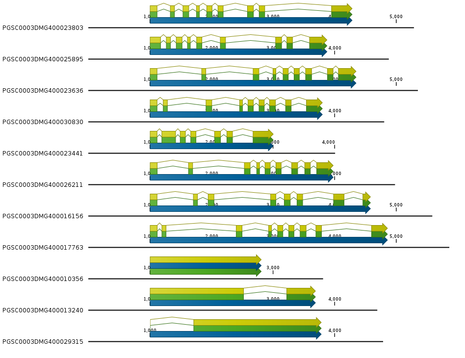 Example of the FASTA file.
>PGSC0003DMG400023803
ACTTGTTGCCACCGCTTCACTCATTTTGACCCGAATCCACCGACAAGGAAAATGTTTTCAATTATTTTTTAAAGAAAACATTTTCTTGTAAAATAAGTTTTTATCTTATTTTCTAGTAATTTCGTAAGCAAGTCTTTTGATCGATGAAACATAACAAAATTAAAAAAATATTTTTTCTCCATACCTAACACAAACGTTGAAATTCGCCACATATTTAAAGGATATTATAATAAATAAATTATTATTACTATCAAATAAACGAATTAATTAGGAAAAATAAAAAGTAAAATAATTTTCTACTACTATAAATAGGGAAGAGATACTTTCATAATGGAATGTAAGACTTTTAACGCATGAGAGCTTTCAATAAAAAAGAAATATTCTTCATTCCTTTTTTTTCACTTTTTTTCTCTTCACCAATTCACACTTTGTCCCTATTACTCCCTAGAATCTCTCGCTCTGTCTCATGCACACACAGACACACACTAGAGGATTCCTTGCTTTAGCTTCAAATCTCTGCTAATAATCTTGATTTCATTTTTCTCTCCTTTTCTCCCACCATAACCCCATATCAATTTTGTTCTACCCATCTTCAAAGGCCCACAATTTCCCAATCTTTGTGCTACAAGAAACCCTAGTTCTTCTAAAATTCACAGATTCTCAAATACCCTTTTCCTGATTTGGTGAATATATGTTGATTTTGGTTCATATTACGTTGTAATTCAGCTTAAAGGTGTTGAATTCAGGTTGGTTTTGGAGTTTGGATTTTGGGATTTTATGGGTATTTTGTAAATTGCTTTAAAGATTGATCTTTTTTTTTGTTAAATTGAAAACCCCCTCATTCCCAATTTTGCATCTTGCAGCAGAATTTGGGTTTGATTGTTGTTTCAAAGGGGAGAAAGTTTGAAGCTCAAGTTTTGGTGGATTTTGTGGTTTTGAATTGAAGGGATTTTTTTTTGTTTTTTTTTATATGTAGTGAAGTTTATTTAAGGATAAGAAGATGGAGAAATACGAGCTTGTGAAGGATATAGGGTCTGGGAATTTTGGTGTTGCAAGGCTCATGAGGAACAAGGAGACCAAAGAACTCGTGGCAATGAAATACATTGAGAGAGGACACAAGGTTTGCATAATTACTGTCTTCTATCATCAATCTAACATCTTCCAATCTTTTTAAATATCTGATGCTCATTGTTTTCGTTATTGTTAGTGTGTTTTTTCCCTCTTAATTATCAGTTAAACATTTTTTAATCAACCAGGTCCCCTGCTCTCTTTTTTATATGCAATATCATATAAGCTTCCTTAGATTTGAGATGCCACTTCTGTTGTAGATTGATGAGAATGTAGCAAGGGAGATCATTAATCATAAATCACTTCGACATCCAAACATAATTCGCTTCAAGGAGGCAAGTGTGTTCATATCATTTACTATTTCGCAATGCCCTATTGCTTTCATGGTGTTTTCAATTGAAAATGGAAAGGAAAGTTGATGAATAACTGGCCTAAACTGTTGTTCATTTGTTTTGTGAGATGCAGGTGGTATTGACTCCCACTCATCTTGCCATTGTTATGGAATATGCAGCTGGGGGAGAACTGTTTGAGCGCATTTGCAATGCAGGAAGGTTCAGTGAAGATGAGGTATAGTTAGAATTTCTAAATTCTGTAATTTTAGAAGGCCACACTTATGGGATCTTAAGAGCCTTGATTCTCTATCTTTAATGCCTCTCTCATTTTGTTCTTGCTTCTGTAATTTTAGGCCAGATACTTTTTCCAGCAGCTTATTTCAGGTGTCCACTACTGTCACAACATGGTGAGCAATATACAAGAATCTACAGAAAATTATTCATTACTGTGAATATATAAAATGCCATCTTTTTAATATAAGGGAGCTTAGTCCTCTTCAAATTTCCATTGCCTCTGCAGCAAATATGTCATAGAGACCTGAAGCTGGAGAATACCCTTCTTGATGGAAGTGCAGCTCCACGCTTGAAGATATGTGATTTTGGATACTCAAAGGTTGATATGTTCTGCTGAATGGTAGATATAGACATACTATCCCCATAGGGATCACTAAGATGCTCATAGTTTTCTTCTGCAAGTGCAGTCGTCCCTGTTGCATTCGAGGCCAAAATCAACTGTTGGGACTCCAGCTTATATTGCTCCAGAGGTCCTCTCCAGAAGGGAATATGATGGCAAGGTAGAGTAATTATGTGATTTTTTACATTTGGTGGAAATGCGTTATGCAAATTATTTTTCTCTGGCATCCATCTGTGTGGAGCTGAATTTGCTACCATATGTGTCATTTATTTTTATGGTATATACTACCTTTCCTCTTATGAGTAGTTAAGAAACTACTATAACTGGTCGCTCTATGACTTGTTAAGAAGCCACTATAACTCGCTCTATACTTGTTAAGAAACCACTATAACTGGTTGTTCTATGACTTGTTGAATTACAGATTATGCTTCCATCTTTGTGTAAATTGCATCTTTTTGCTTACACCCTCCCCTTCTTTCCTAAAGGTAGAGTTTTTTTACTGATCTTTATTCTTAGGCCGTGAACGTTTGCTTGTGATTATTTCAGCTGGCTGATGTCTGGTCATGTGGAGTGACACTTTACGTGATGCTGGTTGGGGCATACCCTTTTGAAGACCAGGAGGATCCAAAGAACTTTAGGAAAACTATTCAAGTGAGTATTTTCAAGTCTTCATATATCCGACGAACTTCATGCGATGCTTACTCCTTTTAATTTGGCTTTGATGTTTCTCTTCCAGCGAATAATGGCGGTACAGTACAAGATTCCTGACTATGTTCACATATCGCAAGATTGTAGGCACCTTCTCTCTCGCATATTTGTTGCCAATTCCGCAAGGGTATGCTCTCTTCTATCTTTATTGGGTGTATTCTAGTGGAAGTTTGCTTGAATTTTCAATGGGCTAACAATCTGATAGAGATGTTTTTTTTGATGAAGAACAATCTGATAGAGATGTTATGTGTTTAATGCATCATTTACTGTTACACAATGGGGTCTATGCATATGGCGTTGTGGTGCCATTTTCATCCATGCACATTTGACAGATTATCCTCCAATTAGGTCATCAGTGTTACCATATACTGTATATTTGAGATCGCCCTTATCTGAGCCAAAGAAAACTATGATATGTTGGATAATTACGTCAACCTTCCAACACCCTTTTTTACTTGATCTGAGCGTCATCCTTGGTCCCAGTAGTAACCCCTGCACTCTAGGAGTGAGTCGGTGTTGCTCATTTAGATGAATGCAACTAGATAATCTTATTCCGTGGTTCTTGTGAGGGTACTCTGTTGTTTAATCCTCCAACTAAATTTGAGTTAAATGTCTAAGACTACAACAATTGCTTGTGTCATTAAGTAAGCAGTGTTGTTTAGTCAGTCGGATCTTATTGCACTTGCCTACCCTATTCTTAAACGATCAGTTCTCCCTCCCCAAAAGGATGACGTTAACTTCTAATAGTGTGTCCTCTAAACAAATGGAGTTGGGATAGTTGTTTTTTAAATTCAGTTGCTACTGTATTAATGATTCCTTGTAACTTGGCTTTACGAAATGAGAGAGAATCAGAATCATCCAGAGGGGAAGTTAAGTGATATCTCAATTTGATGGTAATTTATGATTTTGTAATTGTTCCTATAATTGTAATGGCAGTCTGCATTTGCAATCTTACCCTTGAGAAAAATCTGAATCAACGTCTGCTTCGTCATCTCTTCAAACTTTCAACATTATAAAGTGTGTATAGCTCTGGAACATGTCATAAATAAACAACATATGCACTAGTATTAAATTTTTGCTTTCATTTCTCTGCTCCTGGCATTCTTACCATATTGGAGGGGGGAAAAGAAAAAGGAGGAAGTTATAACATATTTTAAGTAGGAGGATATTGTGGCTTGTCTAATAAGCAGGTTTATTTTGCAGAGAATCACAATCAAAGAAATCAAGTCGCACCCATGGTTTTTGAAGAATTTGCCTAGGGAGTTGACAGAAGCAGCACAGGCAGCTTATTATAGAAAAGAAAACCCGACATTTTCGCTTCAGAGTGTGGAGGAGATCATGAAAATTGTGGAAGAGGCAAAGACCCCTCCTCCAGTTTCCCGTTCAGTATCAGGTTTTGGCTGGGGAGGTGAAGAAGAAGAAGAGGAGAAGGAAGGAGATGTAGAAGAAGAAGTAGAGGAGGAGGAGGATGAAGAAGAAGAAGACGAATATGACAAACAAGTGAAACAAGCACACCAAAGCTTAGGGGAAGTTCGTCTCACCTAAGCGTAAATTATCTTGCTTGCTCGCGGAGAACTGTGGACACACATATAGCCTATTATGTCTTTGGCATTTCCTGTTTGTGTAAAAGTTGTTTCACCTGGGCCTACTTTATCCGTTTTGCTTGTAGAAACCTATTGCTATTAAGTGTGGCATTTCCTGGTCGTGTCAAGATTTTCTTTCTTCTGTTGTGTGGAACTTAAAAGAAGTCTGTAAATTTCGAGTTTTGAGGTAAGGAAGCTTGTGAATTATATTTTCTTAAGACAAAGGCATTGGTGTACTGAAGTTGAACCTTAGATGAGCCTGAGTTACAATTAACAGGAAACTTCGGTAAGTTTTGTTGTATGCATCTTAGATATATGCAGAGAATTTGCATACATGGTCCTTATGGTCTTTCAGTCTTATTTGCTTTTTATGGGTTTTGTTATTACTGTTGATGTTTGAACTCGTCAGTTTTTACATACATTGGATGACAAGCATGGTGGATTCAGAAAAGTAAAGGTAACGTGTTTGGGATTTGAACTTGGAACCTTACAATGAGTTTGGGAAAACCTAAACTATTGAGTTAATTTCTAGTCTTGTGTTAACGGGATTCGGAGCATCACTACCTTTGAAGTAAAGGTATAATCTGCGTACATTCTGTTCTGACCTCGCTTTATGGGACTAGTATGTTGTTGTTAATGAAGAATTAAGATGAGAAGATATATAATCCTAATGGTACAGTTTTTAGAGTCCAATTCATAATATATTTTTTCAATGTGGACAATGACAGCAATGATATTAATCAATTTAGTTAAGGAAGGATTACCTCACAATTAATTATTATTTCAATTCTTCTTTTAACCGATTCATCTAAATTTAGATTTTAATCAAGCAATGTTCAATATTTGATATAGTAATTCAAAATATGAGATGTAAAAATTAGAATAAAGCAGGCCGTTCTTTTGTTAAGAAAAAAAGGTTAGAAAAGCCAAGAGTGAAAGCAAGGTTGAGAAATATGAAATTC
>PGSC0003DMG400025895
TAAAATTTTTCGTGAAATATAAGTAATTGTGCATGGTGGTGAGTGGTGACCAATCCCTGCCCCATACTGCCTCAACTATCAACCAATCAACTCCAGAGATCATGCCTACCTTTTCTCAAAAAAATTTAAAAATGTTGTAAAATTTGTGCAATTGACACCAAATCCTACACCAACACTTGGACGCTTTCTCGTGCTCTGTGTAATAACCTTATCCACCCCCTCCCCCCACCCACAGGCCACAGGGACTCTTTCGTCATTCTCACGCCACTGAACCCAATAAACAAAGGTACTTTTGTCATTAAACTAATTTATTCTCAAATAAACAAAAAAGAAAAATCTGTAATTATTCAACAATATAGGAGAAATATAAAAGAGACAATACTGTAGTCTATGATTTCGTGTTCAAACTCTAATGATATACGTATAAATTTGAATTAACCGGATGAATGAATTTCAAATATTATATTATCATACCTAAAATAGAGTATCTTTTACCAACAAAATGAGTAAAGTAATAAAAAATGATGTCTGCGAGTGTACTTTGGAAACCCAAAGAAGAAGTAGCTGAAAAAACTAATACTAATAAAGAAAGAAAGAAAGAAGAAAAGCAGCTTACTTCACGAGCTCCTCTGAGCACACAACAAAAAAGATATTTATATATATGTTGATGAAGAACACGTCTGCTCAATCAAAACCCTAACAGAACTGCAATCTCATCATCTACTTTAATTTGCTGTAGAGAAGAGAGAGAAGGTAAGTACAGATTTCACGGGATTGAGCTTATCATCACTTGTTGTTGCCGTCCCTGTCTTCAACTACCAACTATACTCAATCCTGTGATTCATATTACTCCACGTAACACTTCTGATTCAATATTTTTTCCTTGATTTGAGAGTCCTTTGTTTGATGCTGGTTTTTTTTTTTTTTTGGGCCTTTTAGGTGGGTTGTAATAATGTGTGAGGTAGCTTGTTCAAGTTAAAAAGAGAGGTTGTGTTAAATTATGGATCGGACGGCAGTGACAGTAGGACCAGGTATGGACGTACCAATCATGCACGATAGTGATAGATATGAACTTGTACGGGATATTGGTGCTGGGAATTTTGGTGTTGCAAGGCTTATGAGAGATAGGCAGACTAATGAACTTGTTGCTGTTAAGTACATCGAGAGAGGTGAGAAGGTTAGTTGAGATTTCACCTTTTTTATTGGATTTGTGAAGATTCAATTTGTTCTGCAAATTACTAGTTATTTGTTGATGAATTGCAGATTGATGAAAACGTTAAGAGAGAAATCATCAACCATAGATCATTGAGGCACCCTAACATAGTCAGATTCAAAGAGGTATTATATCTACTCAAGATAGTTGTTCGATGATGATGACTTAGGTATTCATATTTATAGTTAATTATGGGAAATTTGGTTTTCAGGTCATATTGACACCAACTCATTTGGCTATTGTGATGGAATTTGCATCTGGAGGGGAGCTGTTTGAGCGCATATGTAATGCTGGTCGTTTTAGCGAAGATGAGGTAAGTATTTTAAAAAATGAATTTGGTTGTCATGGCACTTATTCCTGGATATATTTATAGGCTATTAACTGTAATTTTAGGCACGGTTTTTCTTCCAACAACTCATATCAGGGGTCAGCTATTGTCATGCTATGGTAAGTCCACTGTTCTTCTCTGCTTTCATAATTGAAAATCTTTTGAGTTTGTGAAATTTTTAATGATTTGCTTGCAATTGATTCTTTTTATGAAGCAAGTGTGCCATAGAGACTTGAAATTAGAGAATACATTACTGGATGGTAGTCCTGCACCAAGGCTAAAGATTTGTGATTTTGGATATTCTAAGGTATTGTTTTCTTCACTCTGCTATTTTCTGGGACGGTTTTGCCACAAGTTGATTCCTAACCTCCCCCAAAGAAAGAAAACAAATTATTGAGTATTGGATTAAACCGGTCCAAGTAGAGTGAAATGGATAGTGAGGATTCATATGCAGATCCAACTAGTTTGGGATTGAGGCGTTGTTGTTGTATATATGCTGTTATATCTCAATTCCGTCAAGTGTTTGCTTCTTTCTTCTATCCTCCCTTCTCCTTTATTCATATGTCCTTACCGTCATTTTGACTATTGTTGTATGCAGTCCTCAGTGTTGCATTCACAACCAAAGTCAACTGTTGGTACACCTGCATATATTGCTCCAGAAGTGTTATTGAAGAAAGAATATGACGGGAAGGTATATCTTCTTTTTTTTTATTCTTACATAGAGCAGATGGCTGGTTGAGTTAGTATTTGAATAATGACAATATTTTTAATACAATGCTGTTGTGTTGAGAAAGAACTAATTGAACATTTTGAGATGTCGATCATCAGTGTGTGACAATGGTGGGAAATTGGTCAGGGAACACAGTTTTAGGAGTGTTGTTCCTTACTTGGTGTGTGAGGACTTTTCAACTTATGCAGGACTACGTTCAGGCTAACGGAAAGTGCAGCTATCTTTAAAATTAATCTTTTCCGATTTAAGGAAAAAGAAAAGAAAATTATATAGATGCTTAGAAACGAACATCTTTTCTTGATGTTTTTTCCACCAGAAATGCTGTATGTTTTTTTTATGTTCCTCTCTTTATTTCTAAACAGGAAAGTATCAGAGAGATAGACAATTTTGTCATTACGAGGAGGCTAACTTAATGTTACTTTTTTGGATAAAGTAAATGATATAGTGAACCATAAGACCCTAATGTGCAAAATCAACATTTCAATACTCACAATTGAGGGACTTGAAATAGTTTACTGAAGTAATTTCAATCTTCAAAAATGTGGTCAAACTTTTTGCCACTTTGAACAGTTCCTTAGCCATTTTGCTTGTATTGATGTTTGTAACAATTTGACAATGCTTTAGTAAACATTTAGAGCAGTAGAAAATTTTCCATCTTGTTATGGTTTTGATGATTTAACATTTCCTTTTTGTAATCTATTTTATTCACTTAACTTTTTTGATGATCTTGTTAATTGTTTTTCTTCATTTTCTCAAACTAATGCAGATTGCAGATGTCTGGTCTTGTGGAGTGACTTTGTATGTCATGCTGGTGGGTGCATACCCTTTTGAAGACCCAGAGGAACCTAAAAATTTTCGGAAGACAATACAGGTAACTTCTTATGCATATTGTTAGTGCAAAATCCTCATAATCTGTCTTATTTGACTCAAATCATTTCCTGTTATGCAGCGAATCTTGAACGTACAGTATTCAATTCCTGATTATGTACATATCTCTCCTGAATGTCGTCATCTAATATCAAGGATTTTTGTTGCAGATCCTGCAAAGGTAATCTTTTCCACAAATAATTTCAGTGTTCTTTCTTCATATTTTCTTTGGTCATCTTCTGTCTCAATATGTTTAAGGTCTTTCTAGTAATTGTCGGTTGTGGTGTTGTAACACTGTGTTGCATTGCTCATAACTATTTGAACTTCAATCCTGACTTGGTTAGAAAAATCTTATACTCAAGTGTTCTGGAGTTCAATGACTTTTGTTAGAAAATTTCTCTTATGTGAGGTTTCTTTCTTTCATCATGCTTTATTTTTGCATTGCGACAGAGGATATCAATCCCCGAGATCAAGAACCATGAGTGGTTCTTGAAGAACCTACCTGCAGATCTCATGGATAATACTACAAACAACCAGTTTGAGGAGCCAGATCAACGTATGCAGAGCATTGACGAAATCATGCAGATAATAACTGAGGCCACCATTCCTGCTGCTGGGACCAACAGCCTTAATCATTACCTCACTGGAAGCTTGGACATTGACGATGACATGGAAGAAGATTTGGAGAGTGATCCTGACCTCGATATCGATAGCAGTGGAGAGATTGTCTATGCAATGTAAAAGATATGTGGATGTCTAAATTGACAACAGATCAAATATAACTAGTTTGAGTTCCACAGTTCTTAATCAACTGGTCGATCTTTTGGTATCCACTGTTTGTATATGAAATGCAAGTTTGCAGCAATTCTGGTTCTCCTCTCTTTGTTTTCTTTAGTGACTGTTGCTGTTATGTATCGCTTGATTTCACTTTCTAATTAATGTGTGTTATTGCAAAAACTACTGTGTAACGATATAATTTCACAGTAATGCTTACTCTGTAGCTCTAAATTTTCTTCTGTTACTAAATGTAAAATAGTTTTAATCAAATCTTGCATGCATGTGACACTGTTTTGTGAATTGCTTATACATATCTTTCATTTGAATAATAAAAAAAAACGTGGTTACATCTATCTTCTATTAAATGATTACTAGTCATGACTGATGTACAAATACACCTTTACTTTGCTAATTATTTTGTTTTTTAAGTATTAGATGTCATAATGTTGATATGCTATACACAAAGACCAAAGTACACCAAGACTAAAAAAGCTCTTCTTCCGAATCCCTTCATTCCATCTTATAACTTGTGTTTCTCATATAAGGTCCCGAATAACTCTGTCCACTTTCAGAAGTATGTAGCAAGTTCTGGTAGTTCTTCATTTAATTCTCTTGTTACTCCAGTCCCTAACTTGACACCCTAAACAACATATATTTGTATAATATCAATAGGATCAGAAGTTGTATCAAATCGGAAATAGTGACATGTTTCAATTCAAGCTTACAGATTGCTTACTTAAGGTTTATGCCATTCTTGTTTCTTAGGCTTCCTGGAACACTCCCTTTGAGACGGTTGTTTTGGAGAAACCTATAAAACCAGAAATTTCAGTTATGGACTTACAGAAATGAACATTAATCATCAAATATACAAAATCAAAAACTGAGTTAAGTAGATAAAAAAAACAAAGCAGCATACACTTCTCGAAGTTTAGGTAGTTTTCCTAACGATTCAGGGATTGATCCT
>PGSC0003DMG400023636
TATTTATGTATCAAGAGCCTTGTCATTTCGAATTCCGTTGAATGGTTGTAGTTTCGAGACTCACGTCTAGAATAGCCAGGTGAGACATTCGGTTCATGAATCGGAAACAGTTGTTGTCTTTTATCACCGATAAAAATTGTGGTGGAATGAATAAAACTCTCCTGTCTTAATCAATAATCTCGAGTTCGAATGCAAGTTTGGAGTTGAAAAAGGAAATAATGTCATGAAATGTTTTTCCCTTAGTAAAACTTATATAACGTTAATTTAAATCAATCAATTTTAATATAAATACTGAATACCCGCCGAGAAGCCCACCCAAAGAAGCTATAGACTATAATTCTCGTATTTGACAACTAAATTATACTACCACGTTTGAGTTGTGCAACTTGTTTTTGCCTTCCTTTTAATTTCAAGTCATTTGATTGGTGGTGCCCTAATAGGCTGGGTCCCGATGACATATCAAGGATTCAATCGAATCTCCTCCGTTAAAAAATTATAATATTTATCGTCTATTACATAAAACAAACATTTATATGTTCAAAATAATCTAACTTTAAAATTTTCAATTTTATCTTTAATGACATGATTTTATAACCACGATTACAAGTTTCATAATTTTTTTTTTTTTTTTTAACTTTATGTTCGGTCAAATGTCATCACATTAAAAAAATAAAAATACTTCTAGTCCATTGATGACAAAAAATGTTCAAAATTGTTTTCTTATAAATTTCCAAGTATGACATTTAGTATTTTTTTTAAAAAATAAATATTTAAAAACTTTGGCTCCGCCATGGTCCCACCATTTTATGCTCCTTACAAATATAGGAAGCATGTCATTGAGGAAAAACCAAAAATCACAAAGAAAAAAAGTTTCTTTCTTTCCAGTTAGCAAGATATAGACAGCTTCTTCAAAATTTATTTCTAAACAAAATAATTTTTTTATTTTTTTATGTATGATTATTATTTGAGGTATTAATTGAAGCTGAAATATTTATAAAAAATGGAAAGATATGAAATTCAGAAAGACATTGGTTCTGGGAATTTTGGTGTTGCTAAGCTTGTGAAAGATAAATGGAGTGGTGAACTTTTTGCTGTCAAATATATTGAAAGAGGCAAAAAGGTTTCATTTTTATCTCTCTTTTTCATCCAATTCTTTCAAAAACGAAGCTAGGATTTTGAGTTTATGAGTTCTGGATTCTTATAAATGATTTATACATGTTAAGTGGATTTTTAAATCAAGCTATTGAGTTCTGTCGAACCTGGAGATAAAAAGGTTTGATCTTTATCTCTCTTTCATCCAATTCTTCTTAAGGTGGAGCTCGAATTTCGAGTTTATGAGTTTTGGATTGTAAAAAATGTAACTTATTGGATTCTTGATAAGTTATTTATACGTATTAAGTGAATTTTTAATCATAAATACGGCGTTTGAGCCTAGTATAATTGGGTTCTGCAGAACCAGTAGGTGAAGTTGTAGCTCCGCCCCTGAAGTTCTGATCAAGTTTCTCATGATCAGTTTTTCTGAATAAGTACGGAGCTAGAGTTTTGAGTTTATGAATTTTGGATTATAGAAAACAAAGTTTACTGGATTCTTGATAAATGATTTATACATATAAAGTGGATTTTTAAACAGAAATATGGTGTTTTGGGCCTAGCTATTGAGTTCTACCGAACTTGTAGGCAAAACTGTAGCTCCGCCCCTGAAAAAGTACATATTTGGATATATTGAACTCTTCATATTAGGCTGTTACAGAGTTTTTTTTCATTGAAAAGATTATTTTTTGTTACTCTGTTGATTATTTTTTTTCTTCTTTTAATTCATTTGGGTTTTTCTCTGCAGATTGATGAGCATGTTCAAAGGGAAATAATGAATCACAGATCTTTGAGGCACCCGAATATCATTCGATTTAAGGAGGTAATATTTCAGTATTGAATTGATAATGAAATAGAGAAAAACTCGTGATTGGTGTGGAGGGGAAGATTTGTTTATCATATAGTTCAAGAAAAAGTCGTCTCATTTCCTTACTTCGGTCTAGTTTATTCACTTCAAGACTGGTTATGAACGTCACGTAACATCACTCTCAACCAACCTCCACCGTACTTTTGGTTATGTAACCTGGCTTTCTTGGTATGCGAAGTTGGTTATGTAGGCTGACAACTTTTCCTAGGTTGTTCTGATAGGGAAAATAATCGATTAGTAGTACGTTCGAGATTGCCAAAAAATTGTGCTTATTTGAAAGTTAAAGTTGGAGATTTCCCAAAAAATGGCCACTTTGAATCAGATTCCCTAAGTGTTTCTGTCAACTGTTTATTCCACACAAAGTGAAAGTTGGAATTGAATGTTTTTTCATTCTCTTTATTTCTCCACTAAGTGGGAATTTGGAATCATGTAATGAAAAAGATATTTCTAACCAAATTGCCTTAATATTTGATATTATCATTGATCTTATAGTCTCCTTAGTACCAACTTTTTAAGAAGCCTAAGATGCTTTATCGGATTATGTTTTGATTCGCGAGTTGGTTAATTTTACTAGTCGATTGGTCAAAATCCCGGTTCTTGACTTTGTACATGATTCATTTTGTAATTCTCTGTTACTAAGAGGGCTTAAGACTCTGGCTAATTTGATTGAGATGTATAGACCGGAATGCTTATGCAGGTTTTCGTGATTGTGCAGGTATTTCTCACACCAGCTCATCTAGCTATAGTGATGGAATATGCTTCTGGCGGAGAGCTTTTTGAACGAATATGTAATGCTGGAAGATTCAGTGAAGATGAGGTAACACAAGAATCAAGATTTTAGAATTTTCATTTGTTTTTTTGTGATTGTCATTGCTCCATGTAACAGTAAGTCACCAAATTAGTACTACTTCATTTTTGATGAAAATCAAGTGATAAGCGGCTGCTTTCAATCTCATTCCAACGTGTAGCAGTTATTATCTCGAAACTTTATTAGATTTGTTGAGCTTATCTGTCCAAATTGATGTTATTTTTCATCAGGCAAGATTTTTCTTTCAACAACTTATATCAGGAGTGAGTTACTGTCATTCAATGGTATGAATTAGGCCTATGTTATAAGTTTGCTTCAAATTGTTTTTATTCGAGTACATTAATTTACTCTTGGATTATTAGCTTGTGATGTGATCGTTTTCTTGAATTGCAGCAAATCTGCCACAGAGATCTTAAGCTTGAAAACACATTGTTAGACGGGAGCTCTACACAATGTCTGAAAATATGCGATTTTGGCTATTCTAAGGCAATGAAACAGAACTATATGTTCAATCTTTTGATTGGTTTTGTTTCTTGATTCAGTTTCTGAGTTGTGTTAATTCATTGTTTTAGTCAGCAGCATTGCATTCACAACCAAAATCTACAGTTGGAACTCCGGCCTATATCGCACCAGAAGTCTTATCAAGAAAAGAATATGATGGAAAGGTATGACAATTGACCTTTGACATACAACTTCAATTCATAAATTGATTTGTTGACCTAATCTTCAAGATTTTTATGTTATTATTTTGATGTGAAGATAGCAGATGTTTGGTCTTGTGGGGTCACATTATATGTGATGCTGGTTGGTGCATATCCGTTTGAAGATCCTGATGATCCAAGAAACTTCAAGAAGACAATAACTGTAAACTTCTGCTTCATTTCTTTAAAAACCATAGTTGACTTCTTGATTTGCTTGTTAATTTGTCTCAAAGATATGCATTCTTTGACTAGATCTCTACACAAATAGCCGGCCTGATTTATTGGTTACTTTTCCTAGCTGGTATACATAGGTTATACACATCTAAAAACATATATTATACATCTGCTGGCTATTTTTAGTTTAAGCGGTTGGATGGGCAGCTATTTAGTCTAATTCTTCTTTTGTGTGACAGAGGATATTAAGCGTACAGTACTCGATCCCTTACTATGTCCGAGTGTCCAAGGAGTGTAATCACCTCTTATCTCGGATATTCGTTGCTGATCCTGAGAAGGTTGTTACTAGTTCTTAAATCGTTTTGATTTTGCACATTGATCCTAGAATATGCTAATCTTCTAATATTATGCTTGTAGAGGATAACGATCGAAGAAATAAAGAAGCATCCATGGTTCTTAAAGAACTTGCCTAAAGAATTTATGAAAGGAGAGGAAGCTAGTTTAGTACAAATGAATAGTGAAGAAAAGCCATTACAAAGCATTGAAGAAGCATTGGCTATAATTCAAGAAGCAAGAAAACCAGGAGAGGGGTCTAAAGCAAGTGATTATTTTGTTCATAGCAGCATTAGTATGGATCTTGATGATTTTGATACTGATGCTGATTTAGATGATGAGATTGACACAAGTGGTGATTTTGTATGTGCATTATGAGTGCTACTTTTGAACCAGGAGTCTTGGAGCAACGGTAAAGTTTTCACATGTTCAAGTCGTGAAAATAGTCACTAATGCTTGCATTATGATAGACTGTTTGCATCACACTCCCCTACTAACACAAGATGTTTTGTGCACCAGACTGCCCGTTATTGTGAGTGCTACTTTTCTTGGACAAAATGAAAAAGTAATTGCTATTTTAGTCTCTACTTGGCCCTTTAGTGTTTGTACTCTTTTTGTATTTTAGTTTCATAAATCTTCAATTTGATTGGAAGTTGAAGGTCCTTTTTAAAGATACTATATTCAAATATAGTACACCATGTATGACACCAAGGACTCCACGTAGTTTTGTTTGTATTGTTTGAAATTGTAAATGAAAATTGTGCAACTAGTTTTGAGTGTAAATTAAATATAAGATCATTGTCAAGTTTATAATATTACTAAATACTTAGATTAACTAATCCATAAAGAAGTCCTAGTATTGGACCTTTATTAGTACAAGGAACATATAATAAGTAGATTAATTGCTAACCATTGGTTATTGACCTTTGATTTTATTGAGTTTTTTTTCCCCTTTAATGTTGATATTATTTAATTTGTAGAAGTCATTATCACTTTCTATGGAAGGATTTTGCAAGCTGGTGAGACATGGACTTTTTAGCTATTTTCTATCGAATGTCTTGTCATTCAATATAATAATTATTTTCTCTTCTTCGAGTTATATGATATATTTTTTTATTTTTTTTCAAAGAAATGATATATTTTTATATATAAAAACAATTGAACTTTAAACTTTCGTTTTATCCTTATTCAATTTTAGTGAACGAGACCATAAATAAGTTATAGCTAGACAGAATATTTATATTTTTTTTAAACCTCAATCAAAGTGCATCACACATCTTTGAGCACACATAAATTGTGATGAAAACATTTGCTGTCTATATTTGTAAATAATTCTTTTTAAAAATTTAATATGCATATAGAATATGCTGACATTGTT
>PGSC0003DMG400030830
GTCAAGGTCAATAAATAAATAAAAAATGTACTTTTTTCAAGAAATATAAAAAGGAAAATGTTTTTTCGGCATCTTCACACGCCCATGGAAAGTGAATCACAAACGATTTGCCATGTAGGCAAAAAATGCTTAGACGGTTCAAATCTGGGGTGGTAGAGGTGTTCAATAGGTACTAGGTGTAGTTGAGGTGTCTAAATGAATAATGAGGAAAACTTTGAGGGGTCGTAGATAACTTTGACCTTAATAATTTTACCACTAGATCACCACCCGAAAATACCACAACCATCCATTTATAAATCACCTTATACACTTACTACTCAAACTATTATTACAGTAGACAATTGCTATTAGGGAGATCTTCTGTTAGCTCAAGATTGTTACGTAGGATTGAAAGATTCAACTAAAGAAAAGAAAATTAGAAAGGAGAATGAGATTTTCTCATTTTATTTGGATTGATTACAAATGACTAAGATCGTATTTATAAAAAAAAAATACCATTGGTAATTAAAGGTCCTATATCGTTGTACGGTCTAAAATTGTGTTCCAGTTTGATCAAAGAGCCCAAATTCAAAGGAGCAGGACCAACATGAAGAACTCCAATCAATTTATCCACCAATCTAATCACAACTAGTGGCAACTTTTCTGCAGATCTGACCAGACTTTTCTTCTCTTTTTTTTTACATATAATAAAAATATGTACCTGGACTAAGTTTTAGATTCCTATGGGTAAATTCTTATTGAAATTCACCAATTAAAGATAAATGTAAAAGTTCTTCCTACCCACTTGAGCTAATTAGTGACGACAATAGTTGAACAACGTAGTACCTGCCAAGAATGTGTGTCCAATAAACTCTCAGCTAGTAAACCTCTGAATAATTTGAACCCCTTTTGCTCTTACTGTTGAATATTGTCAATTCTGTAAGTCAATAACAGTAGTGGAAAAAAAAAGTTTGATTCTTTCTGAAGAATCTGAAACCCCTTTTGTTTCTTAATCTTGATGATGGAGCGTTATGAGATAGTGAAGGAGTTGGGTTCTGGTAATTTTGGAGTAGCAAAGCTTGTTTGTGACAAGAACACTAAAGAACTCTTTGCTGTTAAGTTTATTGAAAGAGGCCAAAAGGTTTCCCCTCTTTTATAACCTTAAATTTGATGTTTTCACTCTATCTAGGGTACTTTATTTATTTGTTTGTTTGTGTTTTGAGGTTGTTTGCAGATTGATGAACATGTGCAAAGGGAAATCATGAATCATAGATCATTGAAACATCCAAATATAGTGAGATTTAAAGAGGTATATGTTCTGCTTCTTACTAATGGAATGAATCTTCTTTTATCTTTATTCTATAATATGCTTTGATACCTATGGGGGTTCTGATTATTGCTGTCATCAGACTTACAAGGAACTTTCATTAAGTTAAAGATCTTTTTTTTTGAAAGAATTCTTGAGGTATGGAGATAGCTTCACATAATGATAGGATCAAAAATGTTAATGGATCTAATTACTAGAACAGAAGATCTCGTTTGTAATGTAATGACAGTAACAAGATTCTTATTGTTATGTGCTAGTTGTCCCTCATCGGATAAAAGAGAAATGGGAAATGCTAATGAGTGTATAGGCCAAATGGGCTCCCCACCTATCAGACTAGTCTTTTTGGTTGGCCTCTCCTGTTTGGTCTATAACAACTATGTTATGTTATGATTTCTTTTTGAAGAACTCTGTTGCTCGCAATTAAATGCAATCGTATCTTATGGAATAGATTGAAAGCTATCAACTTTTCTGGACAGTAGCTGTAATTTGATGATTTGCATATTATATTTTGTGGTTGATGATAGCAATTTACAATTAGTAGGATTACAGTGGCTGTTCAAAATAGTTTGTTTTTTTACATGAATGGACTTAACACTTCTAGGTCTTGCTTACACCTACTCATCTAGCAATAGTAATGGAGTATGCTGCGGGAGGAGAGCTCTTTGCGAGGATCTGTAATGCTGGAAGATTTAATGAAGATGAGGTAAGGATGATACTTACACTAGATCCCGCAATTAGTCTTGGCTTAGAACAAACAAACTGTGTATTTTTCATTTGATTTTATAATGTTTGCTTATGATAGTCAGATCTTTGCTGCCTCTTTACTTGGTTGGGTTGGGTAATATGCCTTTTACATTCATGGTAAAGTAGTAGTCTACCATGACATTCATATGGTCCTTTGATGTGGGAAGTCCGCTGGGTAGTAGTCTACCATGTCATGGGCTCTGTTGATGAGTGAAACTAAACTCTTAATTTCCAAGAATGCCGTCTTCTAAGTTGAAAGCATAGAGTGATATGCAATGAGAAGTGTCCCTTTAAATATGTTATCAGTTGACTATCTTCTTGTGTTTATGCCAGCTCTTCCGAGCAGACTCTTTTCTAGTTTAAAATCATCTGAGTGGCTTGGTTATATTTATTTTTTACTCAGGCAAGGTTCTTCTTTCAACAATTGATATCAGGGGTTAGCTACTGCCATTTCATGGTACAGCATCAATACTTCTCTTGCTGTGAACTTCGTTCAGTCCTCCTTTTGGGACTTAGTATATCTTTGGTCTTCCGTTGCAGCAAATCTGTCATAGAGATCTCAAATTGGAAAACACGTTACTTGACGGAAGTGCTGCACCACGTGTCAAAATATGTGATTTTGGGTACTCCAAGGTTACTGATCTTTTCTCTAGGTCTTATCAATTCTTACATCTATTCGAGATTTAAGTTCATATAGAATTGCTACATTTGTTTGCAGTCATCCGTCTTTCATTCTCAACCTAAGTCCACTGTGGGGACACCTGCTTATGTAGCACCAGAGGTCCTAACAAGGAAAGAATATGATGGAGAGGTGCTACATCTTTCTTCTTTGTCATAATATTTGTAGTATACACTCATGTCTCCTCCTGTTAATTCTTGAAACTATAGCTTGCAGATGTTTGGTCCTGTGGAGTCACCTTATATGTAATGCTGGTTGGAGCTTATCCATTTCAAGATTCAAGTGATCCCAAAAACTTCACAAAGACTATTTCTGTGAGTGATGACAACATAATCAGATTTCTAGTAGATGAAAAAGAAGCATGCTTTACTCTGAATTTAGTTTATCAGTTTGCTGCATTTATTGTTCATGCAAGTGTGAAGCATTGAAAAATTTACTGCAGCATTATGATTGGCTAGTTTCCATGACAGAAAATACTCACCGCTCGCTACTCAATTCCTGAGCAAATCCAAATTTCCCTTGAATGCCGCCATCTCATAGCCAGGATTTTTGTGGCAGACCCTGAAAAGGTAATAAAATCATATGGTCTTCTGCTGATCATAGAATAGTTCATGCGTTGTGTCCAAGTGAAATATCATTATCAGTAATTAACTCATTGTCTCGATATATATATATGTATTCTGCTTAGGTGCAAGGTTCGTTCCCACCAAAGGCCTTCCATAAACTTGCTTTCGTGTTTCTTGTTTCATGTTATATTGCGAATATAATGTGCCAAAACCATAAATGCATGCTGATTATACTTTTGCAGAGAATAACCATTCCAGAAATAAAAATGCATCCCTGGTTTTTAAAGAACTTACCAGTGGAACTGATGGAAGGAGGAAGTTACCAATGTGCCGATGTAAATAACCCTTCCCAGAGCATGGAAGAAGTTTTGGCGATAATACAAGAGGCTAGAGTTCCTTTGCTGGTTGGAACACATTCTTATGGGGGCAGTATGGAACTTGATGAATTGGACGAAGCTGATATTGAAGATGTAATCGAAACTAGTGCTGATTTTGCTGGTTTACTGTGATGTGTTACACAATGCTGTAATTACCTTAGGGTGAAAGAAGAGAGCAATTGGTAACTGCTGTAATATCCTGAGTAGACACTCAAGAGTTCACCCTTTAAGTTGCTCATAGTTTTTTTTTTTTCCTTTTGACTAAAAGGTGTTTACTACTTTTGAAATCTTGGCTTAGTGGAAATCTGGTCTTTAAACACACACTTGTACCACAAGATAACAGTAGTTTTGTTTAGATTTCTGGAATTAGATCGTTTTTTTTTACACAGTAGAATTTTAGTGGGTGATCCTTTATCGTATATAACAACATTCATATAGGTGAATACAGAGTGATTGACTGAAGTTGCTATTTGCACCAAGTTATCAGTTTAGTTGCATAGATGAGCTGTTTTCGAAAGCAGGACGTGAGTTAAATAAGAAGTCGTAAGAACAACCACCAAGGCTAAGCCTCCTTACTCCACAATCATTGTTTCAAGTTTTTGGTAGATAATGGATTTTGTCAAAGTTTTGAAGAAATGATCAGTAGGAAAAAGGGGGGGAAATATCAATAAATTGCCTCAAACAAATGTTAAGTGCACGCTCGATTGGACTTATTCAGCATTCATCAATAAAACTGAAAGATAAAAATTAAAAAGAACAAAAGAAAGTTCAACAGGAGCCTGTATAACTATTAAGATCTCCCCATACAGCTTCCTCGACTTCTTCCCATGATTTTGCCATCTTCAGTTTCTTCCAAGTACTGAAAATAGCTCCCAGAACATTTTCATCATGCAAAATACAGTAGCACCTGTACAGATAGAATTCATTGAAAGTGAGTTTAAACCACTACTCCATGTACGAATAAGGTGCGACAGGGGGAGTAGTAATAAGTCATATAGAATCAATGGATTCATGAAAAAGTAAAACCCATTGATGACATATTTTATCACAATTAATATTTTTTGGCTAATAGAGGGATCAAATGGTATATAGTTCATTTGTTGGTAGCTTGGAGCATTAAAAGCACACCTCT
>PGSC0003DMG400023441
AAACTAATGAATGGAATAAGGTTTCCTTCATCTTTAACTAAAGTTCTCGAATCCTGGGTACGGAATTGCCAAAGTGCTTTACCTCCTTTCTGCCTCCTTTCCAGTGCAAATCCCGATTTAATTGGACTCCAATATAATTACTAGATATCATTAATTACAATAGATAGCTATATACACATACTGAAGAAACATAAAGCTGATCAGAGTAACATGATCATTATCTGGGAAATGTTGAGATTCAAATAATTCATAGTTATATAGTATGATATATCCAAGCGACCGATTGACCAATAATAATAATAATATATAAATTGCTTAGCAGAAAAGATATATACTACTACTAGTATATAATTATGGTGTAAAACTAAAAGTCAAAAATTGTGACAACCCACATCTGCACTTCCTTGGAGAGCGGCGTTTTTGTAGATCCAAAGCAAATCAATGACGTCTCTTCAACTTTAATTGTCATCATCATGTATACACTAGCTCTTATGTTTGGTTGGAGCCTGGAGGTATTAGATAGTAATTGTAACTTATTCCCAATCAAACGAGTTTAATGTTTTCTTCCCACTAGCTGATTAATTTGTTTAAAATATATATATGGAAGTGGTGATGAGTGGGACTTGGAGTGTGGAATCAATCCCATACCTCTTTACTCTTTACTCCTCCCCGGCCCACCCCCACGTGCTCTTCAGTAGTGTACATGTTAAATATTAATCAAGGGCAGGCTTGATGAACTGCACCTTACCTTTCATATGTATATATATATATATATATATGCCAGTTGCCAGTTGCCAGTTGCCAGTTGCCAGTTTTAATCACTTCATCATGTGTCATCCATAAGTCATAAACTCATCAATCCCACTAGCCACCTATAAATACATCACCTGATCAATCATTTACCAATCTATATTGCCCATATATACAACAAATCCATAGTATATATATATATATATTAATTATAGTAGAAGCTGCAGATATATCGAATTAGCTAGCGACGATGCAGAATTACGAAGTTGTGAAGGAATTGGGATCTGGTAATTTTGGTGTGGCCAGGCTCATGAGGCACAAAGAAACTAAACAGCTTGTTGCGATGAAATACATAGAGCGAGGCCGCAAGGTACCCTGCCCTGCTCTGTCTTTCTGCTTATATATATAAATAATACTAATACTAGTTTAATTTGTTGTAGATTGATGAGAATGTGGCGAGAGAAATCATAAATCACAGATCATTGAGACATCCAAATATTATTCGTTTCAAAGAGGTGTTATTAACATCAACACATTTGGGAATAGTAATGGAGTATGCAGCTGGTGGTGAACTCTTTGATCGCATCTGTCAAGCTGGGAGATTCAGTGAACCTGAAGCTCGATACTTTTTTCAACAGTTGATCTCTGGAGTCCATTACTGCCACAACATGGTACTTCTTTCATTTCTATTATATAGTAGCATCGATCAATCGGTCACTGATAATCAATATTGTACAGCAAATCTGTCACAGAGATCTGAAATTGGAAAACACACTGTTAGATGGAAGTCCAGCACCTCGTCTTAAAATTTGTGACTTTGGTTACTCCAAGGTACTTACATATACTATAAAATTAATTTCATATATTTTCTATATATACCGTACTGATTTAGTCATGATCGCATAACAGTCGTCTGTGTTGCATTCACGTCCCAAGTCGACTGTTGGAACACCAGCCTATATTGCACCCGAGGTTCTATCGCGCCGTGAATATGATGGCAAGGTAACATAGTATGAATCTTTTTGTTGGTTAAAATCTAAGTGAAATACTATACATTGAAGCAATGCAAGTTGTAAAAACAAGCATGTGAAGTTTGCATTATATCATGTGATGGTGACTTATAAAATAATCAATGGACCTTATCCTTGAAGTTAATTATAATTTCTTGAGTGATCCTACTTTCAGCTAGTTAATTAAACATGTCATTTTATTGGTTAAGTATACCTACTCTCCCGGCCTTTATATATCTAATATTTTTTATATGATATTAAAAAGATCTTTTCCTTTTTTTATTAGTCTGCAGATGTATGGTCATGTGGAGTGACTTTATATGTCATGTTGGTGGGAGGATATCCTTTTGAAGATGTAGATGATCCCAAGAATTTCAGAAAAACTATTTCAGTGAGTTTTCTCTCTTTTTAAATAAAATAAAATAAATTGACATATGCACTTTATAATATATATTAATTAATATATGGTGCTTTTCGTTTTTGCAGAGAATAATGGGTGTTCAATACAAAATCCCAGACTACGTCCATATATCTCATGATTGCAAACACCTTCTTTCTCGCATTTTTGTTGCCAGTCCTGCCAGGGTATTATATGATTCATGCAATAAACAATTGTAGTATAATTTATGTTACAACAAATGTGAAATCTATAATATCCAACTTTAAGTGTAGACATTTGAATTTGTATAAAGTTGAACACTAGTATAGGACATGTCTGTCTATCTACTTGTTCAACTTTAAACATGTTTTAGTGTTTATTTATGCACATCCGAAATTGGAAGGCATAGATGTTAGCTGAGGTCAAACTAAAAGGGAAATTCATGTATTATGCCTTCATTAAATGTTGACACTGCTTACTAAAATTTCTACATATGCTGTTGTGTACTAATGTATGATATATGTTGGGGCAGAGAATCACACTAAAAGAGATCAAGAATCATCCATGGTTTTTGAAGAGCTTGCCAAAAGAACTTACAGAATCAGCTCAAGCAGTATATTACAAAAGAGACAATCCAACATTCTCCCTTCAGAGCATTGAGGAGATCATGAAAATTGTATCAGAGGCAAGAAATCCACCACCTCCATCAAGGCCAGTTCCGCACTTTGGCTGGGGAACTGAAGAAGAGGAAGAAGACGGAGAGACCAAAGAAGAAGACGCGGAAGAGGATGAAGAAGATGAGTATGAAAAACAAGTTAAGCAAGTTCATGCAAGTGGAGAGTTTCATATCACACATGATGATGCTTAAGTTTACCATTTCTCATTTTCAGTATAGTCTCTGATTTTGATGTTCTGTACAACTAATAACAGCACTTGGCCTATTTCCTACCATCAACAAACTTTTCAAAAATATTACTAGTATTCCTTCCTTGTATTGAGATTGCAGGGTCAAATGCTTCTATCTGAAAGCCTAATGGAAGGATATCTGCATACTTCTTTCTAAGAAGACATTACACTTAACACTTCACCAGAAATGGGGTTTTCCTAACTGGATATTCCTTTTCTTTCCTTTGGAACTCAAAGCTCTGAACATAATTAGCACAACAAAGACAAGAAGCTGATTTACACCCTTCTAATGGAACGGAAATGATAAGATTGTAATTCATCTCTAATAATCAAACATTAGACAACGGTTGTCGCCCAAAGTTTTAACCAAATACTGAACAATGGCATACCACAATCCTACAACAATTAACTCATTATATTCTCATGACAATCCTCCAAAGAGAAAACAGAGGAAACTTCATACATGCAGATGTCCTTCCCAGCCATCCCAACTACAAAGCGAAGCCCTTCAAATATTCTGGATCTCGCTTTGCACGTTCCTGGAATTTCTTGAACCAGCGATCTAATATATCCATAGGCACCACCAGCTTACTGCCATCCACTCCACAAAATGACTGCATAAAATTGAATAAATTCTCGCCAACTTTCAGTGCCAGCCTCTCAATTTTCTGCCCTGCAGCCACATCAAGGGAGGGAAGTGTTGCAAGATCCTCTACTGAAACACCTATCTTTGCAGAGATTGGAGTTGCATCAGCAGTGAGCTGCAGTTGCCCACCGGGCTCTGGCCAAGGAAGCGACAGCACAGCAGAGGGTCGAGTCAGTGTGACTGCACCACAAAAGAGGAAAGGTGAGCCAGGGGATTGGATATACACAGCGAGGGCCTTGTCTGGTGGCAGCGTGAGGTTGTTGAGGAGGAATATGCAGACCTCTCGAATTGAATCATATGCTTCCCCTGCACATGT
>PGSC0003DMG400026211
TTGGATAATATATTCTTCAATGCTACCCCAAAAGTCACAAACAAGGGGCATTTTCGTATCTGACCAAAACGATTGTGGTACAGTAGTAAGACTATTTCATTCCTAATTAAAAGTTTTGGTTTTGAGCTTTAGGTATTAAAAAAAATTATGTTAAAAGCGTTACTCTCTAATGAATCATGCAATGCGCTTCCAAATTTAATTAAAGCTACAGTACAGACATCAAACATCGAATATAAAACCAAAAACAAGGGTCCCTTTCTCAGCCCACGTTTATTAAAATAGTTGAATTTAAAAATTTACTTTATTTTTTTGGTACATTGAATTCAAAAGTTTATCCCATGCCCAAACTTAAATAATTCATCCACCTCAGCCATAACCAAGCACTTCAACACTTATTGAGCTTTGAAGCCAACCCCTCAAATATTAAATTTGTTAAATTATTTATACGTGCCCTTTAGTTTAACCAATAGAACATTAGATTCTCCAATTGTTTTATGTACATACTTCAACTGATTTTTGCATTTTGTCATCATTTACTATAAATTGCAGTATAACTGAGAGTTGTTGAAAACAAGGATTGGTTAGAAACTGAACTTTTGGTTGTTAAAGGCTGAATTTTTTTGTCTTTCTTGATTTGGTTGGTGAAAAAAGATTTGAGTCTTTTTTGTTATTCTTGATTTGGGTTTCTCTTTTAAAGGAAAAATATTGAATTTTTTTTGCTTATTCTTGATTTGGGTATTTCTTACAAGGGAAAAAGATTGCGTTTTTTTGGTTATTGTTGATTTGGGTATTTCTTACAAGTGAAAAAGATTGAGTCTTTTTGGTTATTCTTGAGTTGGGTATTTCTTTCAAGTGAAAAAGATCGAGTCTTTTTGGTTATTTCTTTCAAGTGAAAAAGATTGAGTCTTTTTGTTATTCTTGATTTGGGTATTTGTGTTCTTTTGAGTTTGAGATTTAAGAGCTTGTGGGTGTGTGATTTAGTGATTTTGGATTGGATAGAATGGAGGAAAAGTATGAGCTTTTGAAGGAACTTGGTGCTGGGAATTTTGGAGTAGCAAGGTTAGTCAAGGATAAGAAGACAAAGGAGCTTTTAGCTGTCAAATATATAGAAAGAGGGAAAAAGGTAAGTTTTTTTGTTATCAAAAAAGTTTGTTTTTGTACTTTTGTTTGTAGATGCTGTCATTATATTTCACTTTGTTAGGTTAAGGATTGTGTTGGATTTGCTTATTTGGTTGATTTTTCTACTGAACTCCTTTACTGGTTCTACTTTAGAATTTGTTAGTTTTGAGGTTTTGGGACTTCTGAGTTTGCAAAGTCAGCTTTTGTGTTTTTTGCAAGAAGTGTTTGCTTGAGCTGAAATGTTGCAAAAAAGAGTTTTTAAAAACTGATTTAGGTTTGAAATGCAGTTGACATTGTGTTGTTGCTCATTCAACTATAAGCCAAAGTAAAAAGGAGCAATTTTGGCCCATTGCAAAAGCTTTTTTAAGTACAATATTTTTCTCCTCATTTACTAAGTTGTATCAAATGCTTTCAGCCTGATGTAGTAGTTATTGTTACAGTATGTAGTGTTTTCTCCTTTGATTCTGTTAGCCTGATGTAAAGGTTGCTTTATTCTTGTCTCAGATTGATGAGAATGTGCAGAGAGAAATTATAAATCATAGATCGTTGAGGCATCCGAACATTGTTAGGTTTAAAGAGGTAAATACTTCCTTTATATTAATTTGTTATGAACCTGAGAATTGCATATATCCATCTGATGTTTACTGTATATGTTCTTTTTTATAATCACATTGTAAGCAACATTATTACCCTTTCTGAAACAAAAGGATTGGACTTGGTAGAGCTTAGCTTGCCAGTTTAGAGATAGCGATCACTATGCTTGTATCGAACCTGGATAGATATGATTATCATATGGGGATGACTTCCCAGATTAAGTGTAAATAGAGATAAATTGCATTAGTTCTCTTTTGTTAGCAGAGTGTATATTGAGTATTTAGCCGACCCTAACTTGTTTGGGACTGAGGCGTAGTTGTTGTTGGAAATAAAAGTACATTTCAATAGTCCTGTTGTTAAGTAAGCAGAGTGTATATGAGTAATTCCTTGCAGTTATTAACTTAAAACTTCAAAACACAATTTACAGGTCCTGTTTTAGTCTATATAGGCATAGCAATTACATAATCCCCTCTTGAGCAACTGTAATATTGAGTGTTAAAGATGGATTTTTGTGGAATGCTAACGATGAGTTCATGGGGATGAAACTTTAGTTAGAGATATTTGATTAACCCAATTTTTGTTGTAGTTGGCCTATGGATTGATTGTTTTCTTCATCTCTTTCTTGTGCACACTATGTACGTTTTTAGATTGCTGAGACTCTGCAATCTAATACACCTATCAACTTCTGTTCTGTTCTATTATTCTCGTTTTGCTGTTCATACTTGTCCATTAGACTACTTGGCACATATATTTAATACAATGTACTCAATGGACCATTACACATTCACAGTTACATGGCATACTCCCTTTTTTGTAGGTCCTGGTTACTCCGTCGCATTTGGCAATTGTTATGGAGTACGCAGCAGGTGGAGAACTTTTTGGTAGAATATGCAGTGCTGGCAGATTTAGTGAAGATGAGGTTAAGCAGATATCTCTAATTCCTCATATTGTTCTATGTTTGATGAGAATGATCATGTTGAACTAATTAACTTCATTTTTTGTGTCAACAAACAACAGGCTCGTTTCTTCTTCCAACAGCTTATATCCGGTGTCAGCTACTGTCATACCATGGTAAATTTGAAAATACATAAACATCTTGTTAAATGCTCATCTTTCTAGTCATTCTCAAATCGTGTTTTTACTTTCTCGTAGGAAATTTGTCACAGGGACTTGAAACTGGAAAACACTCTTCTTGATGGAAGTCCTTCACCACGTTTAAAAATATGCGATTTTGGTTATTCCAAGGTTTGTTCTTGACTTCTAGTTATGAAGTTTACTATGCTACATTTAACATGATGTTAACTTACTTGTATATACTTTATCATGCAGTCTGGTTTGCTGCATTCACAACCAAAGTCGACTGTGGGAACTCCTGCTTACATTGCCCCCGAGGTCCTGTCACGAAAGGAATATGATGGGAAGGCAAGTTCTCTTCTCGGACATTGCTTTAGTTTTGTCACTGATTATTACATTTAACACGACGCTAATATATTTACATATTCATAATGCTTAGTTACATGACTGTATTCTTTTCTTGTTGTTTCACTTGAATGCTGTGCTCATGTTATCGTTATGCATTTTTCAGATCGCAGACGTGTGGTCATGTGGAGTGACACTATATGTAATGTTAGTAGGAGCATACCCTTTTGAGGATCCTGAAGATCCGAAAAACTTCAGGAAAACCATTGGGGTGAGTTGTGTATACTTCTTTCGAATGTTTGAACTAAGTACAAGTGTGTTGAAATTTGTAAACCGTAGTCTCAATTAGCGACTAAAGAATCTTTTATTTGTGTTCAGAGAATAATGAGTGCCCAACACTCCATACCCGACTATGTACGAATCACACCAGATTGCAAGAACCTCCTTTCGCGAATCTTTGTTGCAAATCCCTCTAAGGTAAAACTCATGACTTAACTATGGTTTGTTCATTAACATAACATGTATATTGTTGACTTCAATTTGTGCATTAAACGTTCGAATTCCCTATTCAGAGGATAACTATTCCTGAGATAAAGAAACATCCTTGGTTCTTAAAGAATCTGCCAAAAGAGCTGATGGATGTTGAGCACACGAAATTCGAAGAAGCTTCAGAGCAACTACAACAAAGTGTGGAAGAAATCATGAAGATGATACAAGAAGCTAAAATACCTGGAGTAGTGTCAAAATCTGAAGGGAAAGATCATGCAGGGACAACAGAACAAGATGATTTAGAGGAAGACCTCGAATCGGAAATCGACAGCAGCAATGACTTTGCTGTTTATGTCTGAGGATGATATTTTATGATCAATTGGACTTATAAGAGTAAATGTTTAATTTTTATCTCCTATGAATTGTCTATTATGTTGTACAGAAGAGTTATGCACAGAGCTATTTACTGAGTTCTAAGTGTGCATTTCAAATTTGTTAGATGGATGTAATGTTTGCTACAAACAGATTATGTAACTTTTGAAGTTTTAACCATTTGGTATCTGTCTAATTTGGATTCACGTTGTGTAAGCCCCAAGTGGGGGTAAAGTGGTCTCAATTGTAATGTTCTACCTTTTCAGGGCTAGAAGTTGAAACCTCTTTAGCTTAAATGAAGAGATTATACCATCACATCACAAGTTGTAGTTAGTGTTGGAGTTCGAATTTTCGCTAAGATCGATGAGTTACTTTATGTTAAATGTTAGTTTTCATTCATATATATTAAATTTTGTACACTTTTAGTGAAATTCGTGTCTATAGAAAAGCAAGGCTAAAATGTTCAAGATCGAATGATCTTCAATTAATTCATGCTAATAATGTATGTTGTTATGTGTTCGAATAGTGAAATTAATTATTAATATTTGTATCTGAGTAAACAACCTATATTAAGTGCATGATTCTTCTCTAAACTCGTAAATATGAAATACTTTGTGTACCAGACTGCCTTTAATTTTTGTAATAATGCATACCTAACTTAACAATTTGAAAATAACTTCTTTCATTTTCTAGTCTATTATTTCCAAACTAATTGGCTTCATCGTTAATTCTTATAGTTTATATTAATGGACTAGAAAACAAGTTAATTTATGATCTCAAACTAACTGACTTCATCGTTAATTCTTATTTTATAACATAATATACATGAAATCCTAGCCGCCATAAAATAAAGATTGCCACCAACACAATAAATTGCAATTTATTGAAGGATTAAAAAGAATAATATTGATATCCTCTATTATTGGTGTAAGTACAACTTTACAACCTAAACCTATTTAAAATCAAAATATTATGTATTAAAATAAT
>PGSC0003DMG400016156
GTCAACCCTAATTTAAGGTCCAGTTGAGTCCTTTATGAAAATAAATAAATTCAAATTGATTAAGACCATTTGCTAAATAATCCATATAAACTAAGTAAAACCATATAATATAAGCTTAGAAAAATCATGTTGGCTTCAGAATTTCAAGATTTTAGTTCACAATTTTGCAAAGAATTTACAATATTTGTATCACTAATGTAGCTCCGCGGTCACACAAGGGGGAATTCAAAATTTAAAATTTGAAAATATGGCTTTTAAGATTTTTAATATTGAATTCATATTTTAAAATTATGGATTCAGACTAACTCTTTATTGCAATATTAATGATTATATATTGATTTTCTGCTATACCATTAATATTAAAGTGTTATTGGAAAAAAAGAAAGAAGAATCTCATTCGTTTCATCGCATCACTTTTTTTGTATGGGCGTAGTTAAAGGCAGAAGGGGTTCATCTTGATGAATAGAAAGTCTCACATACGTGAATGAATAGAATTTTGGGATCCTTATAACGGTTCAGATATCTCTTCCCTTTGAGCTAATTTTTGGGACGTAAGTTAGGAACCAAACCAAATTTAACATGGTATCAGAGTCCCGATGTAGACTAGAAAATCGGACTATGTATGGAATGTCGCACATTGAAATCATGACCTCTTTATAAAACTTGGACAATCTTACATCTGGACCTTCTTCGTCAGAAAATTACATTCCTTTTACTAAAAATCCTGAGCCATCATTGATCTTTTGTCATTTTTTTAATGTTAGTTTTCTCTTTTTAGTTTCAGGCATTTAAATATACCACGTTGGTAGATTCAACATATCTTAATTATACTAAAATTTCAATCCATTGGAACAGTGCCACGTGTCTACCATTCTCTAGTGTATGTTCTTGTCAAGTAGGACTTGATCAACAGTTCACTTTAGTTATTATAAATAGTGCCTTACATGTATTATGATTTTTTGTTTTCAAATACTCAAATTATACATTTTTTATTAATATAATGGAAAGGTATGAAATTTTGAAAGATATTGGTTCTGGTAATTTTGGTGTAGCAAAGTTAGTCAAAGATAAGTTGACAAATGAGCTTTATGCTGTCAAGTATATTGAGAGAGGCAAAAAGGTTTGTGTTGCTTCATCTTTTTCCTTTTCGGATTTCGGTATCTACTTTAGAGGTCGAGGATTAGGGTAGAAGGTTCGTAGGTAGCTGAATGTTGTTGCTCGTTGCGTGGGTAGTTATCGTGTAGTTTCTTATCCTTTAATGTGTATTACTATTTGTTGCTTTGGTTGTTTTGTGTTTTCATATTTTACCGTCTTATTTTCTTACAATCCCACATAGAATACTTTTATTTTTGAGGTGACGGTCTATCAAAAATAGCTCCACTCTATAAAGGTAGGGTAAAGGTTTAGGTGTATTCTACCTTCCACAGACATCACTTGTGGATTAAACTGGATATGTTGTTGTTGTTGGAGTTCGGTATCCACTTTATGGGGCTCTAACTAAGCCTGATTCGTGTTGTGTAAGGCCTATTAAAAGGGAAAGCGCTTTCTACCAGGATTTTTTTTTCATATCTAGAACTCGAAACTTTTTGAGTAATTCATAATTCATGTGGTAGTTATGAAGTATGTAAACTTGTTCTTGTTAATTGACAAGATTAATTTTTGCTATTTTTTCTTGATTTATTTTGGTGTTGTATGTGTGCAGATTGATGAGCATGTTCAGAGAGAAATCATGAATCATAGGTCCTTGAAGCATCCCAATATCATTAGATTCAAGGAGGTAATTAATTAATGATGTATTAATTACCTATGTCAACGTCTGGTCTAAAAGCTTAAACTAAAAAAGAGAGCGCACCACACATTTATTCACTTAATTATGTTTTCAACACGTTCTCTCACGTTTGATGGACTAAAGTTTTAAAGCATGTTGTTCATTATTGTGTAGGTATTTCTTACCCCAACTCATCTAGCCATAGTGATGGAATATGCTGCTGGTGGAGAGCTTTTTGAAAGAATATGCAATGCTGGTAGATTCAGTGAAGATGAGGTAACACACAAAAAAAAAAACTGTCGCTCGGATTATCCAAAAATGTTGCCCCACTTGTGTCGTAAAACTGCGCTACTTTTGGAAGATCTCACACGCACCCTGTAGCATTTTTGAAGAGTCTGAGCAAAACATAGATAAGCACTCAAATTAATTCCTCTTCTTCTTGGAAATTTGAGATACGCGCGTCTATTTTTAAATTTTGATCCATCTTTTAGAAGTTCGAATACATATGTGATTATATCAGCACTAACGCATCGAATCTCATCAAACCTCTGAAGTTAAGCATGCTTGAGCCAGAGTAGTACTGAGATGGGAGACTCCTTAGGAATTAAGTTCTCCTGTTACATCCCTCCTTTTATCGAAACTAAGCTTAATTTTGTCTATTTAATTATAATTTTTTGCTTAAAAGGCCCAAATTGTTTTATCAAATATATAATTCAATTTTAGTGTCATTGTATTTTGAGCTCTTTTTTTCATGTTATCTGTCCTGTTTTTTGTTATATTTTTCAGGCAAGATTTTTCTTTCAACAACTTATATCAGGAGTCAGTTACTGTCACTCAATGGTAAAATTGAGACCTATTACTTCATTTGAATTAATTTATTCTTTATTAACTCTTATATGATGCTTGGAGTGCCGTCCTTTTTTGAACTCTGCTAATGCGGGATGCTTCCATACTCATGTTCTATGACATGCATTGTGATGTCCAAATATTTTTTTGAATGCAGCAAATTTGTCATAGAGATCTCAAGCTCGAAAACACTCTCTTAGATGATAGCTCAAAACCGCGTCTTAAAATATGCGATTTTGGCTACTCCAAGGCAATGATCTTGAACTCTACTCTTATGTTGAAATTGGATCATTTTTTCATCAAAATAGTTTCTCATTGTTGTATGTATAATTCATTGTGTAGTCATCAGTCTTGCATTCTCAACCTAAATCTACTGTTGGAACTCCGGCCTATATCGCCCCAGAAGTCTTATTGAGAAAAGAGTACGATGGGAAGGTACAATTATAACGATTTGAGTAATAGTTTTGATCGTATATTGTCAGTATATATAACTTAAATATGTTCATCAATTATTTGTTTGACTTGAACTTCATGGTTTAAATGTCATTATTTTGGATGTAAAAGCTAGCAGATGTTTGGTCTTGTGGGGTAACATTATATGTGATGCTTGTTGGTGCTTATCCTTTTGAAGATCCTGAAGATCCAAGAAATTTCAGGAAAACTTTAACAGTAAGTTATGATTCATTTTTATAAAAAAAAAACGCGTTAATTTCACGTATGGTCATTGAACGTTACTTAGTATAACATACGTGAAATTTTGGTTTATGACAGAGGATATTAAGCGTTCAGTATTCAATCCCTTATTACGTTCGAGTTTCAAAGGAGTGTAAGCTTCTTTTATCTCAAATATTTGTAGCTGACCCTAGCAAGGTTTGTAGTTGTATTTTCACTTCAAATTTGTACATTTTTTTTGTTGTTTTTGGAGGAAAAAATTATTGAAAACACTCCTAAAGTAGGCGTGAATTATTAGTTTCATCTCCGAACTATTTGACAGCCTTAAAAACACCTCTTCACTTGATTAACTGAACTTAAATACATTCCCGATCTTGCAATATGAGTGAATTACATCCTTAAATTCTTGTCAAGTTTAGAGGTATTTTCAACACTTCTGTCGGCTTTTTATTAAGATCTCCATGCCCTTACAAGGGTTTGAGACCACTTGCTATGTCATGTGGCAGAGCGGGGCTGATCAAGGGTGTGTCTAAGTTTAGTTAGTCAAGTAAAGGGGTGTTTTAAGGCTGTTAATAGTTCAAGAATGAAACTAATGATTTGCATCAAGTTTAGAAGTATTTTCAACAATTCTCTCTTGTTTTTTGTTTTGTTGATAAACAACTAATTGTGTTGTATGCTTTTTGTATATGTAGAGAATAACTATTGAAGAGATTAAAAAACATCCTTGGTTTCTAAAGGATTTGCCTATAGAATATATGGAAGGGGAGGATGCAAGTTTACAAATGAAAGAAGAAAATGAACCAACTCAAAGTATTGATGAAGTGTTAGCTATAATTCAAGAGGCAAAAAAACCAGGAGAAGGGCCCAAAGGTTGTGATTTATTGGTCAAGGGAATAAGTAGTAGCATTGATCTTGGTGATGATGATGATTCAGATATTGATGATGATACTGATGATGATATAGAGACAAGTGGGGAATTTGTTTGTGCTTTATGAGTGTTGCATGTGTATAATAGACTCAATGTGATCATACTCATGTGTGGAGATTGATGTAGATTATAAGATAGAGATGAGCGCATGCTTTTTTTTTATCTTTGTATTATGAGTGTTACATGTGTAGATTTGATGTGGTTCGATTGTTTCTTGAATTTTATTGTGTATAATGAAAGCTTTAGTGTGTGCATTAAACGTTCTTTATGATGAGTGTTACTTTACATTGTGCCATGAAGGTCAAAGTCAAAACTATGATGATGATCATTCTTTAGCCATGAAAATGATATTTTTTCCTATGGTTGTTTAACCATGATTAAGTGATATCAGATATGTATTTTCACTTCACTTCGAAATTATGTATAAGATAAAATTTCTTGATTCGGTGAAAACGCCTGTTATCGATAAATATTTACCCTTTTTAGCATAGTGGTTGTAAGTTTTACTCTATGGCTTTTTGCCTTTTACTTAATCTCATATATATTATGTTTATGAAATTCTCTAATTTTGGTAAAGATTATACCATGTAGAAATATTCAATCATGTATGAACCTTTTGATTCTATATAACATTCTTGTAATTGTATATAAACACTACAAGTTGTACTTATGTGATGAACCACAAGTGCATTAGACCAATAAAATGCATAAAGATTTTGTTGTTAATGTATGATAATTCATATATCTGATCCTAACTTATATTCAACGAAACACAATTGTTATTATTCAAATAAATCGATCAACTAAATCGAGAAAATTTTAACCTTACAATAAGAGTATATATACTATTATACCTATATGTCACTTGAACACAATTGCTTGCTCTATGTTCACATCCATTATCTAATGATTATTTCGAATTAGTAACTTTCTTTTTTTTGATTGGTTACAAGATTTCCAGTGTATATATTTTTGAAAAAAAACAGGATAATGTTTTTGTGCTGCTTCTATTAATTCTTATGTGTCCTCCCAATAATTGATATGTGTGTCCCACTTATATATAAGTTAGTAACAATTTTGTGCTATAATAGTTGTCTTTAATTATTGATTCTCTGGCTTGCTAGATCTTGAAGTTTCCCATAATAATGTTAATGGATAGGGCTGACAATATAGAACAAGTAACCATCTAATCCTACCTATTAAATGCATATAATACATCATCTTAAAAATATTTTTAGCGACAATTAATAAATAAAAATAATTAAATATATTCTTTTAGAGGCAGTTAACACTCTTTATAAATGTCCCTAAAATATATAACAATATTGGATCTAATAGCAATTAACTAATGTTGGTAAAGACTTTAGCACT
>PGSC0003DMG400017763
TTAAAAGTGGCAATATATGTAATTGTTTGAAAGTAGAGATAATATTAGTATATATGGTATGGATGTATGTCTAATTAGGTAGTTTTCCCTATTAAAATATATTCAATTTAGTTTAGGACAGGTACAAAGGTGACAAAAATTGGGCCAAAGGCCCAAAACGAAAATAGGCCCAAGTGCTGGCCCAGGCGAACAGATCCAGACTTGGGCCCATATTTTCTTTCCCTATTTACTTGATTGATGTTATGTGCTTATTTGTTAAAAATTAATATTAAGGTTTCAAAACTTCAAATCCCCAAAAGACACCCATTTTAAATTAATTACTTAACTAAATTATTCATTTTTACTTTGACTTAAAAATAAATAAATAAATAAGCATACAAAATACTTCACTTAAATAACATTGCAATATTTTTCAATTTCTCCCTTGAAATGGTCCTAATTATAAAATAATCCAATTTTGTGATTCAAGCTAAATTAAAATTATTTTAGCCAAATAATTAATTGTCGGATAACCGCATTAGCGGATATTCTAGATGCCTTAAAAACCTTCCTAGAATATTAATAGGAACCTCGAACCCCTCTTTAAATATTTTCAATCGATTTCCTGTTTTTATCGTTTGAAAAAATTAGTTTTCTTGATTTTTTCTTAAAAATTAAGTGGCGACTCTTAAATCAGTCCAAAATTATATTTTCCTAATAAAACAATATTTATGTATTATTTAAAGTCTTTATTTGATTTTCTACTTTAGACATAGACATCCTAACTTTTTATCATTACGTGGCTAATTGTCAATTTCCACGCTGATATTAGTGAAAACTTTAGCTGCTCCCAAAAACACGTTTTCTTGTCTTCTTTTGAGTCAGTGGTAAGTCTCAATTTTTCCAAATTATTTTTAGTATGAAATTGCAAGTCAAAGGAAAAAAATTTGCTTCTTTTATGAATTGTGATTTCTGAAAAATCTTGAAATCCCTCTTTTTCTGTGTTTTTTTTTTTGTTATAATGATAGAGGGTTATGAGTTTGTGAAGGATTTGGGTTGTGGTAATTTTGGAGTAGCTAAGCTTGTAAGAGATTATAAGACTAAAGAGCTCTTTGCTGTCAAGTTCTTTGAAAGAGGCCAAAAGGTCAGCAAAACTTTAATAATTTTAGTCATTTGTTTGTTTTTGGATAGTGATTTTATGTGATATTTCAGATTGATGAACATGTACAAAGGGAAATTATGAATCATAGATCATTGAGTCATCCAAATATAATCAGATTCAAAGAGGTAACTCTTGCTAATATTTTACTCTTCAATTCCTTATTAGCTAAGTAACTGCTTTTACGGTTTCAATTTGTTTGTTTTGGTTTTTTAGTCCTTTCGGTCCGTTTAAAAAAAAAATTTCTTTTTAGCAACTTTTTGAAATGTTTAAGACATAGATTAAAAGGTATTTTGCTAGTACTTTTTTAAACTTCATATCAAGTTAACAAGGACAATCAAATTGAAATGAGGGAATATATTGTTGATTCCTCTGGGAATTCTAGATACATATACTCTGTTGCTACGAGAGTGGCTTTCTTTTTTTTACCCGTCCCTAAGAGTTCTCTCTTGTTTTGACTCGAACCCACACCCTTACTATTGGATAGAGGCTGCTTAACATCCGAGCAATGTCCTACGAAAGTGGCTTGATTAAGGTACTTGTAGTTTTAAAGTTGTCTAACCATGTAATCATATTTTTTTCTTTTTGGTCATAGCAATCTTATCTTCCTTCTTTCTTTCTTTCCCTTTTTTGTGTGTGCTGTATCTCAGCCAGTTCCCAAGAAATGTCATTGTTGTTCTTGTTTTTATTCTTATGTTGCAGTTTGTGTGACACATTTTTCTTTGTAGTCCGTTCCAAAAAAAATGACAGGCTAGTGGAGTTGAAAGCAATTAACTTTGCACTTTCTATTTGCCTGTAATGAGAAAGTTGTATAACCACATAAATATTATGACATATTTGAGACGGTAAGTTTCGAAAGTTTTATGGTCACACAAATGGTAGGAGTATGACAAGTTTAAGACCACTAGATTAAAAAATCTCCATTTCAGTCTTAAAATCCCCTGTCGATTTAAACTATGTCACATAAATTGAAACAGATGGAGTAATTATTTTTAGGGGTTAATACTGAGTTGTACGTTAGTTCTGCCTCTGCTTTGAAGGACTCTGCATCTTGCAATTACCAAAATGCAACATTTTGATTCTTATGGAAATGAATTTATCGATCCTTTTGATTTATTTTGTGCTGGGATTCCTTATGTCTTCTAACAGTAGGTTCAACGAATTCGAGTGAAATGAAGTACAACATGTAGTTAAGCAGCATGTACGCATGATTTCTATTATGTTTATGGCTTTTTGAATTAATGGACTCACCTCGACCAGGTTTTGCTGACGCCTACTCATCTAGCAATAGTAATGGAGTATGCGGCAGGAGGAGAACTCTTTCAGAGGATTTGTAAAGCTGGAAGATTTAACGAAAACGAGGTAATAAACGATAATTAAAGCGTGATTCTTCCCGCTTATGACTTGGCTAGATCAAAATTTTCATTTTACAGATTTCTATTGATTATTATTTACTTCTGACAAACAACTCAGTGTGTGTTGTGTGTGCGTGTGTGGGGGATTGTCATTCTTCTTATTTACCTGTCTTCATTGCACATCCACATCCCTTTTCGTATTGATACTCCATAGAGTACTACGTGTTGACGTAGTTATAGAGGCAGACTTAAATGCTCTTCACTGGAAATATGGATTACAAACTTCCGAGTATTAATGACATATCGAATGTTGAAACCAAAACTTGTTATGCCTTGAAAATTCTCATGTTTCGAGTTCATTATTCACGATGTTTGTATGCGTGTGTGCATGTGGACATTTTAATTTGCTTATTTATTTTGTTTTTGGTCAGGCAAGATTCTTCTTTCAACAATTGATATCAGGGGTTAGCTACTGCCATTTCATGGTAAAACATGGATATTAATTTCTCACACTTTCAAGTTTCGTTTCGTTTTTATTTTTCTTAGACCTGTTATGTTAATTGCTCTTTGGTTGCAGCAAATCTGTCATAGAGATCTCAAATTGGAAAATACGTTACTAGACGGAAGTACTGCACCTCGCGTAAAAATATGTGATTTTGGTTACTCCAAGGTCAATATAATCTTTTGTCATACCTTAATTCTAACTACAATTTCAGATTTTCGTTGAGCTCGTGTAACAGACTTCACTTGTCTGCAGTCATCTGTCTTTCATTCTCAACCAAAGTCCACTGTAGGGACACCAGCTTACGTTGCACCGGAGATCTTATCAAAGAAAGAATATGACGGGAAGGTACTAGTCATTTCATGTTCTCGTGTCAGCAGTTTCATAATGCTTGTATCATTTAACCGTTTTTTCGTTCTTGTTAATTATTGAGTTCATAGGTTGCAGATGTTTGGTCTTGTGGAGTCACTTTATACGTAATGCTGGTCGGAGCTTATCCATTTGAAGATCCCACTGATCCAAAAAACATCAGAAAGACCATATCTGTGAGTATATGAAAAAAAAATACATTTCTGTTATATACATAAAGTCGAACTTGATCGACTTATAGAAAAAGGAAAAAGAAACTGCTCCGATTTGAATGTCGTAACGTCGATTGAATGCACCATTCTGATTGAGTTTAATCCTCCGTAACAGAGAATATTTAGCGTCCAGTACTCAATTCCACAAAATGTCCGAATTTCTGTGGAGTGCCAGCATCTCTTATCCCGGATTTTTGTAGCAGACCCTGAAAAGGTAAATATTAATATACTCTTCTGCCAAAAAAAGCATTATATCATCATAAATCCAGTATGTGAAATGTTGTTTGGGTGAGTGACACGATCAGTCGGTCACGAATGACATATTTACCTCATCATATCAGCAGAGACAGATCTAGGATTTGAAATTTTTGATTTCTTTCAACGACATCAAGTTAATATAGTGAGTTCACAATCATATATTTATAGATATTTAGCGAATTCAGGCAAAAGTTACTGGGCTCACGTGAACCCACATATTACATTGTAAATACTCCCCTGCATCTTAGTATTTCCTATCGAAAATCACAGTCGTCCTAGGCATTTCAAGTTTTCATTTCACTACATTATACTTGGAAGGAAGGAGTGGAGGTCACGTATTAGGGTAGAAACTTAGTAGGGGTAGAGTGTTGTCTTGCCTTGCGAAGGTTCCTTGTAGTTATTGTCATATGTTGTTTATTGTGTTTTGATAATCACACTATTTGCTACTGTTACTGTTCTTCCTTATAAACATTGGACTACTTTTCTTGTTAACTGCTATGCTTCTTCATTGTTTTCATCTTTTGTGCTCGAGTTTGATGTACCTAAGCTGAGGATCAATCGGAAACAACCTCTCTAACTTCACGAGGTAGTGGTAAGATATGCGTACACTCTACCCTCCCCAAACCCCACTTAGTGGGATTTCACTGGGTATGTTGTATGCTTGGACGTGCCTCCATGTGTAATTTTTTTGAGTCCTAAGCTAGAACCTGTGTGTTCGGAATAGTCTAATCTTATTAGTGGCTTACTGGTTCTTTTGCAGAGAATAACCATCCCAGAAATTAAGAACCATCCTTGGTTTTTGAAGAACTTGCCTGTCGAATTCATGGAAGAAGGACGGAACGAGTGCATCGGTGTAAATAACCCGAGACAGAGCATGGAAGAAGTATTGGCAGTAATACAGGAAGCAAGAATTGCTTTGCAGGTTCTAGCAAGTTCATCTCAAGGCATTATGGAAGAATTTGATGAATTAGATGATGCTGATATAGAAGATATTGAAACAAGTGGTGACTTTCTTTGTTATTTGTGATGTTTAATTTGTGTCAGATATTTTGTAATATATAGAGGTTTTAGATTGAACAAACACATTTGTTCATTAAAGAACATGACTATTATGAAATGTCATTTGTTCATGAAAGAAAATGATTATTATGCAAAGTCATCTCTTAACTTCTGGATTCTTTATGAGTAGCCTAAGAATAAAATTTGCACATATATACAAGGGTTTTGTTGTATCTTGAAGGGAATTGCTTGTATTTTCACTAATATGTATACATACAATATCTCTTTAAGGAAAATGATTCTTCACGCCTCAAAAGTCATCTTCTTTTTCAATTATTTTTCTAACAATCTTAAAGAGATATTGGGTTTGAAGAAGATAGAAACAACTATGACAATCCAAAAATGGTGTTGCACTCCGAGAAGTAAGGATTTCCATTTTTAAGGAAAAATATTGATGATGATAACCCTAAATTAAGAAATAATACCAACGATTTTGATATCTGAGATGGCAAAAGTGATCACAAGAGCAATGGATCAAGAAGGAAGCGATCAAAATCGGGTTCTACTATCTTAAGTTTGCGTATTAATTAATTATTTTATCCTTTGAGATTTTGAGAAGTTATTTTCATAAGTATTAGGATAAATAATTCACTTGTGATGATCTTGAAATACATTTTAAATAAGTTTAGGATTGACATATTTGGTTTGCTTATTATAAATTTGCTATTTGGGACAAAGAAAAATATTATAGCATAATTGTGTTGCATAAAGATCATGTAAATTTTAATTTCAAGTTATGAAATAGTATATGAATTTAGTTATTTTGCTAGATAATATCTATACGTGAAAGTTATTAGAATAATTTAAAATTAAGAGAAATGATAATTTTTATTAGATCATGCCTTTAGTAAAGGTTGAAGACTGTCTTCTTATTAAATGCTCGTGTATTATAGTATTGGAACACAATAAACTTGACAACAAGATGATCTACTGACGTTAATTATATGTCCGCACAAGTTACCAAAAAG
>PGSC0003DMG400010356
ATGAGATGGGAGGGAGAATATATATATAATATGAGGGTCGATTCACATGAGAACTGTTTTGATTCGCCTCAAATTATTCATAGCAGTAAGTGAAAAATGATTCCCCAAATTAGCCTTGTCACAGTGAGTGTGATATCATTGCACCTTTTCAACTACGATAGCAACTGTTGTAGTGACAAAATTGACAGACACTAATCAACTAACATTATGGGAAATATCTATAATGTTCCTCACTAGAAACCAATGCCTTCATCCATGGTTGATTTACTTATAACTTTGTATATACTCATTCACTTTTACTTATCACATTATGCTCATTAAAAAAATAATGATCGATATGACTATCTTGCCATACTACCCCTATTAATTGATGTTTAGTTTAAGTCAAAAAATAAGTAATTAATGTTAAGGACAAAACACTAGAAAAAAAAATAACTGTCTTTTCTTGATATGTTAAAATTGACAAACAAAAGTGAAAATCTAATTTTGAAATAGTGGACAAGTAAAAGTGATCGGAGAGAGTATCTGAATCTGTGCTATTCTTTTGCATATTCTTGTATTGAAGTTCATCAAAAAGGTTTAAAAGAAAGAGAGGAAGTTGGAGTAAAGGATCCCATAATAATGATAGAAGAAACACAAGAAAAGGATCATATTCAAGTAAGGGACACTTGACATCAGAGGAAGGTACATCCTTAAACATTGTTCACAAAATTTCAGGTCTTCCTTTTTCATCTCCGATTACTCGATACATATAATTTCTACATGCAAAACACGATCGAGAATAAATATCATTTCACCAATTCTTCATTGATCAAATACTTGAAACATTTGCTAGGCAGGAATGATGTCTATAAATCATATCAAGGCTGCCTGGATTGCCTATAATGTGCAATCTTTTTGCATTCTAAGCCTCTTAATCCAAGCTCTATTGCTTCTTTTAGCACCATTCAGGAAGAGAACAGGCAGTAAAATCCTGATGGTGTTTGTTTGGTCAGCATACATGGCTGCTGATTGGGCCCCTGCTTTCATTCTCAATCTCATTGTAAATTACAGCAAAACAAGACATGACAAGACAGAACTTATGTCATTTTGGGCTTCTTGTATGTTGTTGCATTTAGGAGGTTCTGATCATGCAATAGCATTTTCCCTCGAGGACAATGACCTGTGGTTTAGGTATGCTTTCACGTTTGTTTTCATGTTCCTGTCCTCTGCCTACGTGTTCTACTTATCGTTCTCCCAAGTAAACTATCTTTGGATCCCAAATGTCCTAGTGTTCCTGGCTGGAATCATCAAATGTTACGAGAGGGCACGTGCTAGGTTCATTGGGAGTATGGATAAGTCCATAACATTGAGTAATCCTAAGTACGAAGATGTTGTGAAGAGGAAGTCGTCAGAAGAACCTCACAATTTCCGAGCAGGAGAGCTGGATGATGTGGAGGTTATACAACTTGCATATACAATATTCAGGGCCTATAAAGGTGTTCTGGTGGAGCACAAGTTCACTTTTGAGGAGTATGGTAGAATTCAACAACTCTTGCAAAACAGAACTGATCTGTTTGCTTTTAGAATCGCGCAGGCTGAACTCGAGATTCTACATGATGTTCTATACACTAAGGCCCAAATTTTCCATGAAAGTTTTGGGAACTCAGCTCGATCTGTCTATTGGGTTCTGCTTCCTGCAGCATTGGCCTCTTTCTCTTTGTTGGTGAGGAACAACAAGCAAAAGCAATTTGATCCGTTCGATGTAGGACTAACCTATAGCTTACTCATTGGAGGTATGTTTTTGGATGCCATTGCTTTTGTTATCTTGCTTTATTCCTCAACTTTCACAATTGCCACAATGTCAAGGGCAACGTCGAGGCCAATCACTTGGGTGGTCAAATTCCTCAAAGCTTTAAAGTGGCCACGGCCACGTGCTCTATGGTGTTGGAGACCATCTCTCCAACAATTCAACCTCATAACCTATGGTTTAAATCGACCTCCAAAAGCATGGGAATGCATAATTGATTCCCTACACCTTACAAATTATCTTGATGAGATGATATATGTGAAAAACAAGAGTCTTTCTCCTATATTGGAAGCTGAAATTCTAAGACAAGTAGAAATACGTCTAAATAGGCATGATTGGGATTGTAACTCGTATGCTTCTACATTCACTAAATGCACCAGCAAGTTCCCTGTGTCGAAGGAGCTTGACAAGAACGAGTTCCTCATAGTATGGCACATTGTGACGGAGATTTTCTATAATGTTGTGGATGTACCTGAGGAAAATATTGGACCTGATTCAAGAGAGTTGAACAAGTTTAGAGAATGTTCAAAGTCTCTATCAGACTACATGATTTACATTCTTATTTTTCGCCCTTTCTTCATGCCTGTTCCTAACAAGAAGAAGATAGAAGAGACCAACAACAAGATAAAAGAATTGCTTCATGAAAAGAAAAATTCAAGCCAACAAGAAGCTTGCCAAGAGATCATGAAAAAAGCTGCTGAGGGGAGAATTCCTCAGGAATCGTTCTTGTATGAAGCTTTTAAGGTTGTCAACTGTTTGCAAACTGAATCTCCTTGGTGTCAAGACAGAGTTAAATGTTGGGAGATTATTCATAAAACTTGGATCGCGATATTATTTGATGCTGCCAAATGCTCTGCACCGCGTGCTCATGCACAATATCTTGTGAGAGGTGGTGAAATTTTATCCTTAATCTGGTTGTTGGGTGCTAACTGTGGATCCATGGCTCAGTTTTCATTTTTTGAAGATTCTGATGAGGAAAATCAAGCTAGTAATATGGCTAGGCTCGAATCGATATATTACTAAAGTTTAGGAATGTAACATATCATGTGAAGAAGAGCATCATACCAGTTGGTCTTAGGATATGGTATCTTTTGTAGTGTTGAAACTTTGTTGTTGTTATGAATAAATTGAGCTAATGGATGTTCATTGAGTACTTTTTTTGAAACATTTGAGTACTTTTACATATTATTTATACCATGAACCATGTAATTTTACATGGACGATGTACTTAATTCTTGTGAATTCTGGGGGAATTTTGTGTCATATAGAGTTCCTTATGTTAAAAGCTTACCCACACCTAGTGTTTATTACACCAAACCATACTAATTTACATGGTCAAGTCATATATTAAGGTGATAATATGTATAATCAGTTAAATTTTTACTGTATTCCTACCCTACGAGAAACATAATTGAATGAAATTATCTAATAGTAACAATCTCCACACTTCTTTTTTCCATCTAAGCATCTCTAATTTTTCTTGTTTTACAAGCTACTAGTATGAGTCTCTAGTCAACTTCAAGTAGAGGTTCATGTTTCTCGATAACATGTTATCAATACGAGTCTCTACTCAACTTCAAATAGAGATTTATATTTTTTTGGTGACTTTTGTATTATAGAAGATGTTAGCAATAGGATTTCCACGCCACAGATGGGAGGTTCTTAAGCCAAAAACAGACACAAGAATATATGCTTTCTTTTAAAAATTCTAACTTGGTTACCACTCAGAGCAGCAGCATATATCTGGTTTTAAGATAGATTACTCTTGACTTTGAGAATTTTCTTTGCAAAAAATATCATCATTTGTAAGCTTATCAAGGCAATTGATTTCTACATGAATTGTGCAATACTTCCCAAAAGAGCAAAACCAAAGAACAACAGCAGTAGCAGCAACAATATTAGTCGTCTTCCGCGTAAATTGGAAGAAATCTTACAATATGCAGAGCCTGGTGTGGAAGTACTTTTGGATGGACAAATCAGGGTATATGTATATCCCCAATTACAAAACTATCCATGTTTTATA
>PGSC0003DMG400013240
TTAACCATGTACACGTTTTGTTTCCCCACTTGCATTTACACGTTTTGTTTCCCATATAAAAGTTGTAGCTTTATGTTGTTTCTCTAAGCTAATTTGTGTGGTAGGACGTATCGTAAATAGTCTCTCTACCTTATAAAGATAGTGGTAAGGTCTGCGTACACTCACCCTGTATAATGTTGTTGTTGTTGATTTTTCATAGTCAATGTTTCTATTAACTTTTTGTTTTTGCTTGCCTTTTTCTTATCATCAACATAAGGTCCATTACATATATTTGCTGATAAATTGTGGAGCAAGAAGTGATTTTTCTGTATATTTCTAGCATTAAGGTCAGTAAAACTGATTAAGTTTCACTTTTATTTTCCTTAGTTTTTGTTATTCTTATTTTTGTTCATGGCATTGTTCATTAAAAGCAACCTTATGTTGTATATGTATTCATTTGCCATTTGCATGGATTTTTTTATATATAAATTTATGCTATGTATTGAAAGTACTAAGTTCAGATGAACTCGACAGGGTGTGCTACATCCGCCTTTCTATATATAAAGAAATCCGCTAAATATGTATAAATATTTGATTATGAACACAGTTATTGTTGTAGAGTGTAGACTAACTTGAGTTCGGCGTGGCTGGAGGAATCCATAAACTTCAACTACTGGATCGCCCTTTGCTTATGATTAATTGTTGTTTCCTTTGTTTTTTTTTTATCTGATTTCTTCATGATATCTCTGGAGAACTTCTTTGTTCTCTTGAAGTTTAATCATACTATATAGTCACATATAAAAAGGACAGTCTGGTGCACAAAGCACATGCACATCCCAGGTTAGAAGGGTCTGAGGAAGGCCGCTTTTTGACTAACTTCAAAGTTTGGGTTCAAACATAATAAGTTTCTGTTCTGTTTGAGTTAGATATCTTTCCATGTGTCTCTGGGATTCTGTTTTTCTGTGAATTTAGTGTGTTGCTGTCTGTTGTTTTCCTGCAGAATTCAGTTCCTCGGGGAAAGATGAAGATCGATAAGTTCATAGATAACATCAAACTTCTGTTTCACCAATGGGAATTGGGATATTCCATTATGTTTAGCATAACATTGCAGGCTTTTCTTATATTTTGGACATACAAAAGAAGGAATTTAGTTGGAACCGTGAGAAAGACGTTGTGGCTTGGGATTTTCCTTGCTGCTGATTTCGTTGCAACGTTGTGTCTAGGAGCCATCTTTCACTTGCCTTTGGGACCGAGTGTGTCATCATCACCTGATGATCATAACAAAAAAATCAAGAACCTTTTGATTATCTGGTCACCCTTCATCCTACTACACTTGGGCAGGCACAGTACACTTGTAGGAATTTCCTTGGCAGATAATGAATTCTGGCTGAGCCATTTCTTTAAATTTTTATACTATGAGTTCATAGCTCTGACGATAAGTATTCTGGGATCCTCGACAAGATGGTTCACTTTGGCATCGCGCATCATGTTGGTTGGAGGCTCTTTAAAGTTTGCTGAAAGAGTTTTGGCGCATAAAAAAGGAAGCATGGATGAGCTCCGTAGATCCATTTTCAAGGAAAATGGCCCCGGTGGCCTTGGCATTTTGGAAATCAATCAAATATTAGATCGTCTCATTAGCGCACATAGACAAGGCCATCTTCAAGAACAATTTCACAATGAAGAAAATGATCATCTAGCCGATGATGCTAACAATGAAGCTGATGTTCTTCCTGTGGCCTCCAGGGAAGCAAATGTAGTAGCCCTGTGTGAAGCTTATCATGCTTTCAACAAGCACAAAGACCTGTATGTTGAAAGTAGGTCGTACGAAGATTGCTACAGGATTAGAGGTGGGCGTTGGCGCGGAGAAACTTTTAACCTCGTTGATGCTGCTACTGCTTTCAACAACATAAAGATGGAACTATGTTTTGCATATGACCATTTCTACACAAAAATGGCATTCTTGCATACTTGGTGGGGCTGGATTGCCCGATTTGTAAGCTTACTTTCAGTATTTATCGCGCTTATCCTGTTTTCTGTTGGAGTTTTCACCAACGATGAATTTAACCGAGCAGACAACTTTGACAAAATTGTCACCTTTCTCCTGATAATTATGGCATTCCTCCTTGAGGCAGGGAGTTTGATTGAGTCCATACTGTCGAAACGCTTTTTGGTGCAGATAGGGATCCGTAAGGGGAAAATGTGGCGTCTTTTGGAAGGATTTATTGTAAGGCTTCCAGGTAGATGTATAATCACCCGAGACAAAAATCCTACCTTAAAGATAGGACAGTTCAGCTTACTTCCTTACTGCTTTAATGATTCCAAGCAGAATGCCCCTTTTAAAAAGTTCTTAGGCTATTTTGATCTGAAACAGTTCTGGAATAACCTTAACTACATTAGCCGTATCTCCATTGAAGACGTTTATGATCATCGGCCCGATGAGGAAAGCAAATTCCTAAATTTGGTCTTTGACTGTATTGCACAACGACTAAGGAGAGAGCGGATGGAGGATGATCACTTCAGGTTCCAATCTCTCATCAGCACAGCTGTGCGTGACCAAATACCTGATCATTTCTTCGAATCCACGAATTTTGAAGAATGTGTTATAGTTTGGCACATAGCCACAGATGTGTGCTACAGACAGTGGCGGAGGCAGGAATTCTATCAAGGGGGTTCAAATAAAAAAAATGTTGTTGCTTGGAATCGAACCCGTGACCCAAAGCTCACATAGGCTGAATCCTGACCCCCATAAACCACTGAGCTACTCCTTTGACATATGCTCAGGGGGTTCAATTTTAAATATATACACGTACACAAAAAAATTGATCGTATATATATAGTGTAATTTTTTTTCCGAGGGGGGTCGGATGACCCCCCTGGACACACTATAGATCCGCCCCTGCAAATAATAGTGTAATGACCTGATTCCATCGTTATGGAAAAGCCAACAGGGAAAAATTTTGGGCAGGAAAATAATTTTGGTAGTAACTTGAGAATTCATTGCCTAGTCCAGTTTTGGACGAAATTGGAGTCAGTGAGGTCTAGGGAAATCTGGTAATACTCCTTTGACATATGCTCAGGGGGTTCAATTTTAAATATATACACGTACACAAAAAAATTGATCGTATATATATAGTGTAATTTTTTTTCCGAGGGGGGTCGGATGACCCCCCTGGACACACTATAGATCCGCCCCTGGCTACAGATTATACTATCACTTGGAGGAATCACATTATCTTCAGTATGCCAAGTACCTCTCAGACTACATGTTATATCTACTGCAAGTTCATCCAGAGATACTGTCACCACTGACAAGAAAAGAGCTACAAAGCTATCGAAATGTATGTGATGCAACTAACAGATTCTATGATGACATGGAGATTCAGAGTCAGGTAATAACAGAGATCGTCGATAAGATTGAACCTGCATACACTAATTTACGTGGAATCCCAAGAGAGAGACGACCAAGGAACATCTCTAACTTGTTACTAGATGGCTATGAACTAGCTCGAGAGATGGGTTGTCAACGTATCCGGGAGTATAGGCTAGGTGAAGAAGTGGATAACACATGGAGAGTGTTATTTGAAGTCTGGGTGGATATACTATCCTATTCTGCAGTTTTTGTTCCAGGGAAACAACACGCTGAGCATCTTGTCACCGGTGGAGAGTTCATAACATATATCTGGTTGCTTATCGTCTACTTGATCGAGAACTGATCGATTATTATTGTTTTTTTTCTTTGTTTAAACTTTCTCTCCAGTTCAATGTATACTTGGATGCTATGTACTGGGGGAAAATGCTGTTACAAAATAAGATGTTGAATGATCAAGAAAGCTTTTCATTTTATTCACTGAACCAAAGGAGTATCTATTTACAGTACAAAGAGCGCTAGTAATAGGAAATATACAATAAAGAAAGACAGAAATAAAAACAGAATAAAGCATTGTTGTATTAAGGTATTTTGATGATTCAACAAACTATGGTAAGTTAGGATCTGGTAAAGGAACCTGATCCTTCGAGCTGAGGCCGCACACGACAACTCAATGGGGTGCAGCTGTAAAGCTGGCAAAACTGCAGAGGTAGGTGGGCACGACAACAGAGGGTTCTCGGCCAATGGCGAGCTACTAGGTTGTTTTGTCTTTCTTATTCATTAGACACATTGACAAGAAACAACCTAGCGTTTGCAAATGAAAGATATTCAAAGCAAAAGTCATTCTCTCAAGGAAGAACTATTCTCAAGCAGCAAGGGACCTGATCAAGTCATCTACAGAAGTTTTAAATTATCATTTGAGTTTAGTGTCTTGTGTTTGTATGTTATAAGATCTATTCCTACGTTATAAAGGAAATCAGATCATGTCAGTTTAAATTGCAAAAGAGTTGAGTTCATCGCTATAGTTAGGCAAGTTGTGTTTGTTTGAAGTCTATGTTAACTAGAGGTAGTTGATATAATAGGCAATAGGGTTATTGCTTTGTATCTTGTAATAGAGGTGTTATAAGGTGTGTAGGATTAAGAGTTAATCCTTTGTGATCACAAGAGTCTGTACTCGCAAGTTGCTTAAAGTTAGTGGAGTTTTGAGAAATCTTGTGTGACAGGCCGTGGTTTTTTCCTCCCTTGAGCAAGAAGGTTTCCACGTAAACTTCCTTGTTCAATTTGGAGATAAGATATGGATGTGCTCGTATCATCGCCTTTGTAAACTGTTACAGAATCACTACAGA
>PGSC0003DMG400029315
AAATTAGTAAGATACAATGATTTTGATATAATTAAAATTATCCTTCATCAAATCTCAAACCATTCTTCAAATTAATAAATATTAATTTATCGATTAAATAATATCTCTATAAAATAATAAATCTTCATGGTCCTAGCTATATTAATTTATAGAGGTTTTACTGTATATATAAAAAAAATTACAATAAATTCAATATTTAATAGTTAATAATTTATGTATTGTGATCTCTACATAACTAAATAATACTTGCATAACTAATACATGCATAACTAAACCCTGCATAATTAATACATGCATAACTAAAACCTACATAAATAAACCCTGCATAACTAAACTATGCATAATTAATACCTACATAACTAATACTTGCATAACTAAATTTTGCATAACTAATACCTACATAACTAAACCCTGCATAGCTAATACCTGCATAACTCTAATCAGTAACCAAACGGCCCCTAAATGTATTAGTTAGTATCTTAAATATTACAAGAAGATACTTCAAAATGCAAGGTAAATATTCATGGTCAAGAATTTTTCAATGAGCTATTAATCAATATCCTGTAAAAAGGAATGTCAAACCATAAATAATTTGAACTTTATAGGTTATGGATTCTAGGACAACGAACTCAACTGCTCGTTTAGGTTTCTAAATTCAACTTTTGTACATATTTAATAAATTTCTTCGCGCATATACATGATTTCACCCAAGCTAGTGGATTTTACCGAACCCATATCCTGAAGACTACCTCCATCCCTTTGTGAGTCCGAGTCAACTTTATATAATAGTCAAGTCTTGTTATGTTCCTAGTTTGTGGTCCCCCCNNNNNNNCGCCCCCCCCCCCCCCCCCACTAAGTTGACTCAACAAGTCTTCTAATGGTACTTCCAAGTTGTTTCCTTTTTCTTTCTTTCTTTTCCAAATACCTGTGATTATAAGTAGTAGTAACATTTTCATCCATTGCAGTAACCAGCTGCCGGGAAGCAATTTATTGATAAACCATGCTTTTACTAGGTACTGTTTGTTTCTGCTTATTGTTCTTGCTTCATCTAATTTTGTTTCAAAGTCAGTGTTGAAAATGTTAATTTAAAGTTTTAAGTGTCTGCTACTCAATCTAGGTGTGTTGTTAGAGTCATTCGAGAATGTTTAGTAATTATGGTTCGTGAAATTGAACGTTTAATGGTTAATATTGTTGCTTTATATATATGGGAGGATAGCGTGTTGTTTTGTAAGAGTGGGGTTTTTCTAATGATATAGGTTTGCTTTATATTTATTTCCCTTTTCCATACTCATTGTGCCTTATATTATGAAGATCCCACCTTATAGTTGTTAGAGCGGATTAGAGTCTCATATTGATTGGGGAATGAACTGATTTTTTGTTTATATGGACTTAGGCAGCTCTCCCCCTCATGAGCTAGTTTTTGTGGTTGAGTTAGGCTCGGATGTCATAACTTTACATGATATATCAGAGCCAGATCTATTTCCGATTGAGCATGGTCTAGTCGGGTCTGGGCGTGAAGGGGTGGGGGGGGGGGGTGTTAAAGTGGGTTAGAGTCCCATGTAGATTGGGAAATGGGCTGATGGTTTGTTTCTATGGATTTGGGAAATGTTCCCTTCATGAACTAGCTTTTGGGGTTGAGTTAGGCTCGGGTGTCATGTTCTTACAATATTCTGACTTAGTTTTCTAATTTTTATCTTTGTTTTGGCAGCTGCAAGTGTAATATTTGTTAATGCTGAGAGAAGAAGGCTAATTGAAGTTATTCCGGACAGCTTGAAGAAAGCATGGAAAGATTGGGAACTAGAAGTGCTGATTCTAGGAAGCCTTATCCTTCAGATTGTGCTTATTCTTTTTGGCAAACACAGGCAGCGTGTGGCGAAATTATGGATCAGAATGACTCTATGGACATCTTACTTACTAGCAGATTGGATTGCTATTGTTGCATTAGGTATCATCTCTCAGAATACGTTGGATAAATGCAAACAAACAAGTGTTGATGACAAGTTAAAGGATGAATTGATGTCGTTCTGGGCGCCATTTATGCTGCTGCATCTTGGCGGTCCTGATACTATCACGGCTTATTCATTGGAGGATAACGAGCTGTGGTTAAGGCATTTAGTCGGTCTGATAATCCAGAGTGGACTAACCTTCTATATCTTGCTTGTGTCCTTGCCAGGCTCTTCTTGGCTTCCATTTCTAAGCTTATTCATCTTCATATCTGGTCTTATCAAGTTCTCTGAGCGGACATGTGCTCTCCGTTCAGCAAAAATCGAGAATCTCAGGGACGCAATGCTGACATCCCCTGATCCTGGACCAAATTATGCTAAATTCATGGAGGAATATACTTTGAAGAAAGCTGAGGGCTTCTACGTGATGGCGGATGAGGTTAAAGAAATCTCACTTCCAATTGATCATTCTTACGATACTGGTAAAGATAAATTGCTGCTGATATCTGAAGCTTTCGATCAGTTCCAGACTTTTAAACGTCTATTTGTGGATCTCATCCTTAGCTTCCAGGACAGAGACAACAGTCGATTTTACTTCAAGCAACTTCCTCCAAAAGAAGCTTTTGATGTGATTGAGGCAGAGTTAGGATTTGCATACGATTCCTTTTATACCAAAGCACCCGCCATTTTTACTCCTCTAGGCTGCATTCTTCGTGTGGTTACTTTTTCTTGCATTTTTTTTAGCTTGATTTCATTTTCTTTATGTAAGGAAAGATCGAAATACCACATACTTGACTTGATTCTCACTTACCTGCTGCTGGTGGTGGCCTTTCTCCTGGAAATATATGCATTGATCGTTTTGCTGAACTCAGACTGGACAAAGAATTGGCTGAGCAAAGGGAAACAGGACGGAAAGTTTTACCAGTCGTTCCTCCTCAACAAGCTGTGTCTGCGAAGATCAAATAAAATGAGGTGGTCCAATTGCACACCCCAATACAATTTGTTGAGCTACTGTGTTGAGTTCAAGCCCCCCCGGTGCTACAGGTTCCAAAAACTCTTTCTAATCAATGAGCTCTTGGAAAAACACAAGTACAAGAAGGATGAACTAGTCACCCCGGAGTTAAAAGAGCTGATCTTTAACCATTTCCAAAAGTTTGCCGGAGAAAGTGATAACGAGCCTGATCATCCAGTCTTATGCACAAGTAGAGGCACTAAAGCACTTACCAAAAATGACTGTTCTTCCCTAGTTTGGTCTACCGAGGTAGAATTTGATCAAAGCTTCCTTATTTGGCACATTGCTACTGATCTATGCTATTACACTGATGATGGAAGTACTCCTCGTTCCATCAAATCCAAGCAAATTAGCAAGCAGTTATCAGATTATATGTTGTATCTTTTAGTAGTATGCCCCTTTATGCTGCCAATAGGACTTGGGATGATCAGATTTAGAGATACATGTGCTGAAGCCAAAGAGTTTTTTACAGAGAGGAAAGTCGGAAAAGACTTAGCTATAGCTAGTCGCAAGTTGCTAACAGTGAATACTGAAGTTAGACCTGCAAAAGTGAAAGGGGATAGGAGCAAGAGCGTGTTGTTTGACGCGTGCATACTTGCCAAATCATTGAAAGAAAAGGGTACTCAGAGAAAATGGGAAATCATCAGTGAAGTATGGGTGGAAATGCTTGCTTATGCTGCTACACATTGCAGAGGGAACCATCACGCTCAACAACTACGTAAAGGAGGAGAGCTTCTTACTCATGTCTGGCTTCTCATGGCACATCTTGGCATCACAGAGCAATTCCAGATAAACAGAGGTCATGCTAGGGCCAAGCTCATTGTCAAGTAATAAACTCGGATTCTCGTGCTGATCAAGACTTAGTAGGTAAATAAATGTGTGTTCTCTCTAATCGTTTTAAGTTTTTTATCATGATATTATAGTAGAGACAGGCTCAGAAAACAAAGTTAACTTTTAGCATGTACCTGTACTTGTTGTAACTAGTTTCTGGTAACGTACATCGCACGTTTGTTCTTTATTATTATGATTAATAAATTTTTTATCTATAATAGTTTTGAGTTATAAAATGGAAATATTGATGGAGTCAGGAGTGATTTTTTTTTTTTGAGAATTGGTAACATGTCAAGAGTGAAAATTGTTAACCACTAACTAATAATCTCGTTTACAGCTTATATGTTATATTCAAATTCAATTTCTATTATATGTATTTCTCTTTAAGATTGTTATTCCTTTTTCATATTTAGAAGGGATAAGGGTCTGAAAAATACCTCAACTTTGATTGAATTTGTTGTTGCGATACTAAACTTTCATGAGGACCTATTACCTCCCTAGACTATTTAATACCGTATTTTAAACATATATATTTGTCCACGTGGACATAAAAAATAATGCAAAATTATAAATAGTAATGTGTCCACGTGAGCACATATATACCTTTAAAATACACTATTAAATAGTTCAGGGGGTAAAAANNNNNNNNNNNNNNNNNNNNNNNNNNNNNNNNNNNNNNNNNNNNNNCTAGAGAGGTAATAAGTCCTCATGAAAGTTTAGTATCGCAACAACAAATTCGACCAAAGTTAGGATATTTTTCAGACCCTTATCCCTATATAGAAAGATAAATTTTAATGTTGTTCATATTTGATTTTTAAGTACTCATTCATATTAAATTAAATAACCTCATTTGTTAGAATATGTCTTCTTCAGAGATTTTCTCGATTTCTTTTGCTCGATGTTGTTGAGGGAGAAGCATTAGTTATCCTTTTTAACTCGAAATCTAGGAGACTAAAAGCAAAATATAATTTCAATAATTCATTGTCAAACTAAAGCTATC
Example of the FASTA file.Example of the GFF file.
PGSC0003DMG400023803
JGI v4.03
gene
1001
4287
.
+
.
ID=PGSC0003DMG400023803;id=PGSC0003DMG400023803.v4.03;pacid=37440166;uniprot=J9ULI1;Name=PGSC0003DMG400023803;gene_id=PGSC0003DMG400023803
PGSC0003DMG400023803
JGI v4.03
mRNA
1001
4287
.
+
.
ID=PGSC0003DMT400061170;Parent=PGSC0003DMG400023803;Name=PGSC0003DMG400023803;gene_id=PGSC0003DMG400023803
PGSC0003DMG400023803
JGI v4.03
exon
1001
1120
.
+
.
ID=PGSC0003DMT400061170:exon:1;Parent=PGSC0003DMT400061170;Name=PGSC0003DMG400023803;gene_id=PGSC0003DMG400023803
PGSC0003DMG400023803
JGI v4.03
CDS
1001
1120
.
+
0
ID=PGSC0003DMT400061170:CDS;Parent=PGSC0003DMT400061170;Name=PGSC0003DMG400023803;gene_id=PGSC0003DMG400023803
PGSC0003DMG400023803
JGI v4.03
exon
1329
1403
.
+
.
ID=PGSC0003DMT400061170:exon:2;Parent=PGSC0003DMT400061170;Name=PGSC0003DMG400023803;gene_id=PGSC0003DMG400023803
PGSC0003DMG400023803
JGI v4.03
CDS
1329
1403
.
+
0
ID=PGSC0003DMT400061170:CDS;Parent=PGSC0003DMT400061170;Name=PGSC0003DMG400023803;gene_id=PGSC0003DMG400023803
PGSC0003DMG400023803
JGI v4.03
exon
1534
1635
.
+
.
ID=PGSC0003DMT400061170:exon:3;Parent=PGSC0003DMT400061170;Name=PGSC0003DMG400023803;gene_id=PGSC0003DMG400023803
PGSC0003DMG400023803
JGI v4.03
CDS
1534
1635
.
+
0
ID=PGSC0003DMT400061170:CDS;Parent=PGSC0003DMT400061170;Name=PGSC0003DMG400023803;gene_id=PGSC0003DMG400023803
PGSC0003DMG400023803
JGI v4.03
exon
1754
1807
.
+
.
ID=PGSC0003DMT400061170:exon:4;Parent=PGSC0003DMT400061170;Name=PGSC0003DMG400023803;gene_id=PGSC0003DMG400023803
PGSC0003DMG400023803
JGI v4.03
CDS
1754
1807
.
+
0
ID=PGSC0003DMT400061170:CDS;Parent=PGSC0003DMT400061170;Name=PGSC0003DMG400023803;gene_id=PGSC0003DMG400023803
PGSC0003DMG400023803
JGI v4.03
exon
1921
2013
.
+
.
ID=PGSC0003DMT400061170:exon:5;Parent=PGSC0003DMT400061170;Name=PGSC0003DMG400023803;gene_id=PGSC0003DMG400023803
PGSC0003DMG400023803
JGI v4.03
CDS
1921
2013
.
+
0
ID=PGSC0003DMT400061170:CDS;Parent=PGSC0003DMT400061170;Name=PGSC0003DMG400023803;gene_id=PGSC0003DMG400023803
PGSC0003DMG400023803
JGI v4.03
exon
2102
2194
.
+
.
ID=PGSC0003DMT400061170:exon:6;Parent=PGSC0003DMT400061170;Name=PGSC0003DMG400023803;gene_id=PGSC0003DMG400023803
PGSC0003DMG400023803
JGI v4.03
CDS
2102
2194
.
+
0
ID=PGSC0003DMT400061170:CDS;Parent=PGSC0003DMT400061170;Name=PGSC0003DMG400023803;gene_id=PGSC0003DMG400023803
PGSC0003DMG400023803
JGI v4.03
exon
2581
2685
.
+
.
ID=PGSC0003DMT400061170:exon:7;Parent=PGSC0003DMT400061170;Name=PGSC0003DMG400023803;gene_id=PGSC0003DMG400023803
PGSC0003DMG400023803
JGI v4.03
CDS
2581
2685
.
+
0
ID=PGSC0003DMT400061170:CDS;Parent=PGSC0003DMT400061170;Name=PGSC0003DMG400023803;gene_id=PGSC0003DMG400023803
PGSC0003DMG400023803
JGI v4.03
exon
2771
2869
.
+
.
ID=PGSC0003DMT400061170:exon:8;Parent=PGSC0003DMT400061170;Name=PGSC0003DMG400023803;gene_id=PGSC0003DMG400023803
PGSC0003DMG400023803
JGI v4.03
CDS
2771
2869
.
+
0
ID=PGSC0003DMT400061170:CDS;Parent=PGSC0003DMT400061170;Name=PGSC0003DMG400023803;gene_id=PGSC0003DMG400023803
PGSC0003DMG400023803
JGI v4.03
exon
3946
4287
.
+
.
ID=PGSC0003DMT400061170:exon:9;Parent=PGSC0003DMT400061170;Name=PGSC0003DMG400023803;gene_id=PGSC0003DMG400023803
PGSC0003DMG400023803
JGI v4.03
CDS
3946
4287
.
+
0
ID=PGSC0003DMT400061170:CDS;Parent=PGSC0003DMT400061170;Name=PGSC0003DMG400023803;gene_id=PGSC0003DMG400023803
PGSC0003DMG400025895
JGI v4.03
gene
1001
3879
.
+
.
ID=PGSC0003DMG400025895;pacid=37436441;id=PGSC0003DMG400025895.v4.03;uniprot=M1CFW5;Name=PGSC0003DMG400025895;gene_id=PGSC0003DMG400025895
PGSC0003DMG400025895
JGI v4.03
mRNA
1001
3879
.
+
.
ID=PGSC0003DMT400066617;Parent=PGSC0003DMG400025895;Name=PGSC0003DMG400025895;gene_id=PGSC0003DMG400025895
PGSC0003DMG400025895
JGI v4.03
exon
3589
3879
.
+
.
ID=PGSC0003DMT400066617:exon:1;Parent=PGSC0003DMT400066617;Name=PGSC0003DMG400025895;gene_id=PGSC0003DMG400025895
PGSC0003DMG400025895
JGI v4.03
CDS
3589
3879
.
+
0
ID=PGSC0003DMT400066617:CDS;Parent=PGSC0003DMT400066617;Name=PGSC0003DMG400025895;gene_id=PGSC0003DMG400025895
PGSC0003DMG400025895
JGI v4.03
exon
3221
3319
.
+
.
ID=PGSC0003DMT400066617:exon:2;Parent=PGSC0003DMT400066617;Name=PGSC0003DMG400025895;gene_id=PGSC0003DMG400025895
PGSC0003DMG400025895
JGI v4.03
CDS
3221
3319
.
+
0
ID=PGSC0003DMT400066617:CDS;Parent=PGSC0003DMT400066617;Name=PGSC0003DMG400025895;gene_id=PGSC0003DMG400025895
PGSC0003DMG400025895
JGI v4.03
exon
3038
3142
.
+
.
ID=PGSC0003DMT400066617:exon:3;Parent=PGSC0003DMT400066617;Name=PGSC0003DMG400025895;gene_id=PGSC0003DMG400025895
PGSC0003DMG400025895
JGI v4.03
CDS
3038
3142
.
+
0
ID=PGSC0003DMT400066617:CDS;Parent=PGSC0003DMT400066617;Name=PGSC0003DMG400025895;gene_id=PGSC0003DMG400025895
PGSC0003DMG400025895
JGI v4.03
exon
2140
2232
.
+
.
ID=PGSC0003DMT400066617:exon:4;Parent=PGSC0003DMT400066617;Name=PGSC0003DMG400025895;gene_id=PGSC0003DMG400025895
PGSC0003DMG400025895
JGI v4.03
CDS
2140
2232
.
+
0
ID=PGSC0003DMT400066617:CDS;Parent=PGSC0003DMT400066617;Name=PGSC0003DMG400025895;gene_id=PGSC0003DMG400025895
PGSC0003DMG400025895
JGI v4.03
exon
1756
1848
.
+
.
ID=PGSC0003DMT400066617:exon:5;Parent=PGSC0003DMT400066617;Name=PGSC0003DMG400025895;gene_id=PGSC0003DMG400025895
PGSC0003DMG400025895
JGI v4.03
CDS
1756
1848
.
+
0
ID=PGSC0003DMT400066617:CDS;Parent=PGSC0003DMT400066617;Name=PGSC0003DMG400025895;gene_id=PGSC0003DMG400025895
PGSC0003DMG400025895
JGI v4.03
exon
1607
1660
.
+
.
ID=PGSC0003DMT400066617:exon:6;Parent=PGSC0003DMT400066617;Name=PGSC0003DMG400025895;gene_id=PGSC0003DMG400025895
PGSC0003DMG400025895
JGI v4.03
CDS
1607
1660
.
+
0
ID=PGSC0003DMT400066617:CDS;Parent=PGSC0003DMT400066617;Name=PGSC0003DMG400025895;gene_id=PGSC0003DMG400025895
PGSC0003DMG400025895
JGI v4.03
exon
1425
1526
.
+
.
ID=PGSC0003DMT400066617:exon:7;Parent=PGSC0003DMT400066617;Name=PGSC0003DMG400025895;gene_id=PGSC0003DMG400025895
PGSC0003DMG400025895
JGI v4.03
CDS
1425
1526
.
+
0
ID=PGSC0003DMT400066617:CDS;Parent=PGSC0003DMT400066617;Name=PGSC0003DMG400025895;gene_id=PGSC0003DMG400025895
PGSC0003DMG400025895
JGI v4.03
exon
1264
1338
.
+
.
ID=PGSC0003DMT400066617:exon:8;Parent=PGSC0003DMT400066617;Name=PGSC0003DMG400025895;gene_id=PGSC0003DMG400025895
PGSC0003DMG400025895
JGI v4.03
CDS
1264
1338
.
+
0
ID=PGSC0003DMT400066617:CDS;Parent=PGSC0003DMT400066617;Name=PGSC0003DMG400025895;gene_id=PGSC0003DMG400025895
PGSC0003DMG400025895
JGI v4.03
exon
1001
1177
.
+
.
ID=PGSC0003DMT400066617:exon:9;Parent=PGSC0003DMT400066617;Name=PGSC0003DMG400025895;gene_id=PGSC0003DMG400025895
PGSC0003DMG400025895
JGI v4.03
CDS
1001
1177
.
+
0
ID=PGSC0003DMT400066617:CDS;Parent=PGSC0003DMT400066617;Name=PGSC0003DMG400025895;gene_id=PGSC0003DMG400025895
PGSC0003DMG400023636
JGI v4.03
gene
1001
4351
.
+
.
ID=PGSC0003DMG400023636;id=PGSC0003DMG400023636.v4.03;pacid=37472637;uniprot=M1C6E4;Name=PGSC0003DMG400023636;gene_id=PGSC0003DMG400023636
PGSC0003DMG400023636
JGI v4.03
mRNA
1001
4351
.
+
.
ID=PGSC0003DMT400060762;Parent=PGSC0003DMG400023636;Name=PGSC0003DMG400023636;gene_id=PGSC0003DMG400023636
PGSC0003DMG400023636
JGI v4.03
exon
1001
1120
.
+
.
ID=PGSC0003DMT400060762:exon:1;Parent=PGSC0003DMT400060762;Name=PGSC0003DMG400023636;gene_id=PGSC0003DMG400023636
PGSC0003DMG400023636
JGI v4.03
CDS
1001
1120
.
+
0
ID=PGSC0003DMT400060762:CDS;Parent=PGSC0003DMT400060762;Name=PGSC0003DMG400023636;gene_id=PGSC0003DMG400023636
PGSC0003DMG400023636
JGI v4.03
exon
1838
1912
.
+
.
ID=PGSC0003DMT400060762:exon:2;Parent=PGSC0003DMT400060762;Name=PGSC0003DMG400023636;gene_id=PGSC0003DMG400023636
PGSC0003DMG400023636
JGI v4.03
CDS
1838
1912
.
+
0
ID=PGSC0003DMT400060762:CDS;Parent=PGSC0003DMT400060762;Name=PGSC0003DMG400023636;gene_id=PGSC0003DMG400023636
PGSC0003DMG400023636
JGI v4.03
exon
2673
2774
.
+
.
ID=PGSC0003DMT400060762:exon:3;Parent=PGSC0003DMT400060762;Name=PGSC0003DMG400023636;gene_id=PGSC0003DMG400023636
PGSC0003DMG400023636
JGI v4.03
CDS
2673
2774
.
+
0
ID=PGSC0003DMT400060762:CDS;Parent=PGSC0003DMT400060762;Name=PGSC0003DMG400023636;gene_id=PGSC0003DMG400023636
PGSC0003DMG400023636
JGI v4.03
exon
2996
3049
.
+
.
ID=PGSC0003DMT400060762:exon:4;Parent=PGSC0003DMT400060762;Name=PGSC0003DMG400023636;gene_id=PGSC0003DMG400023636
PGSC0003DMG400023636
JGI v4.03
CDS
2996
3049
.
+
0
ID=PGSC0003DMT400060762:CDS;Parent=PGSC0003DMT400060762;Name=PGSC0003DMG400023636;gene_id=PGSC0003DMG400023636
PGSC0003DMG400023636
JGI v4.03
exon
3159
3251
.
+
.
ID=PGSC0003DMT400060762:exon:5;Parent=PGSC0003DMT400060762;Name=PGSC0003DMG400023636;gene_id=PGSC0003DMG400023636
PGSC0003DMG400023636
JGI v4.03
CDS
3159
3251
.
+
0
ID=PGSC0003DMT400060762:CDS;Parent=PGSC0003DMT400060762;Name=PGSC0003DMG400023636;gene_id=PGSC0003DMG400023636
PGSC0003DMG400023636
JGI v4.03
exon
3338
3430
.
+
.
ID=PGSC0003DMT400060762:exon:6;Parent=PGSC0003DMT400060762;Name=PGSC0003DMG400023636;gene_id=PGSC0003DMG400023636
PGSC0003DMG400023636
JGI v4.03
CDS
3338
3430
.
+
0
ID=PGSC0003DMT400060762:CDS;Parent=PGSC0003DMT400060762;Name=PGSC0003DMG400023636;gene_id=PGSC0003DMG400023636
PGSC0003DMG400023636
JGI v4.03
exon
3525
3629
.
+
.
ID=PGSC0003DMT400060762:exon:7;Parent=PGSC0003DMT400060762;Name=PGSC0003DMG400023636;gene_id=PGSC0003DMG400023636
PGSC0003DMG400023636
JGI v4.03
CDS
3525
3629
.
+
0
ID=PGSC0003DMT400060762:CDS;Parent=PGSC0003DMT400060762;Name=PGSC0003DMG400023636;gene_id=PGSC0003DMG400023636
PGSC0003DMG400023636
JGI v4.03
exon
3880
3978
.
+
.
ID=PGSC0003DMT400060762:exon:8;Parent=PGSC0003DMT400060762;Name=PGSC0003DMG400023636;gene_id=PGSC0003DMG400023636
PGSC0003DMG400023636
JGI v4.03
CDS
3880
3978
.
+
0
ID=PGSC0003DMT400060762:CDS;Parent=PGSC0003DMT400060762;Name=PGSC0003DMG400023636;gene_id=PGSC0003DMG400023636
PGSC0003DMG400023636
JGI v4.03
exon
4058
4351
.
+
.
ID=PGSC0003DMT400060762:exon:9;Parent=PGSC0003DMT400060762;Name=PGSC0003DMG400023636;gene_id=PGSC0003DMG400023636
PGSC0003DMG400023636
JGI v4.03
CDS
4058
4351
.
+
0
ID=PGSC0003DMT400060762:CDS;Parent=PGSC0003DMT400060762;Name=PGSC0003DMG400023636;gene_id=PGSC0003DMG400023636
PGSC0003DMG400030830
JGI v4.03
gene
1001
3804
.
+
.
ID=PGSC0003DMG400030830;uniprot=M1D1F6;pacid=37475155;id=PGSC0003DMG400030830.v4.03;Name=PGSC0003DMG400030830;gene_id=PGSC0003DMG400030830
PGSC0003DMG400030830
JGI v4.03
mRNA
1001
3804
.
+
.
ID=PGSC0003DMT400079214;Parent=PGSC0003DMG400030830;Name=PGSC0003DMG400030830;gene_id=PGSC0003DMG400030830
PGSC0003DMG400030830
JGI v4.03
exon
3538
3804
.
+
.
ID=PGSC0003DMT400079214:exon:1;Parent=PGSC0003DMT400079214;Name=PGSC0003DMG400030830;gene_id=PGSC0003DMG400030830
PGSC0003DMG400030830
JGI v4.03
CDS
3538
3804
.
+
0
ID=PGSC0003DMT400079214:CDS;Parent=PGSC0003DMT400079214;Name=PGSC0003DMG400030830;gene_id=PGSC0003DMG400030830
PGSC0003DMG400030830
JGI v4.03
exon
3200
3298
.
+
.
ID=PGSC0003DMT400079214:exon:2;Parent=PGSC0003DMT400079214;Name=PGSC0003DMG400030830;gene_id=PGSC0003DMG400030830
PGSC0003DMG400030830
JGI v4.03
CDS
3200
3298
.
+
0
ID=PGSC0003DMT400079214:CDS;Parent=PGSC0003DMT400079214;Name=PGSC0003DMG400030830;gene_id=PGSC0003DMG400030830
PGSC0003DMG400030830
JGI v4.03
exon
2939
3043
.
+
.
ID=PGSC0003DMT400079214:exon:3;Parent=PGSC0003DMT400079214;Name=PGSC0003DMG400030830;gene_id=PGSC0003DMG400030830
PGSC0003DMG400030830
JGI v4.03
CDS
2939
3043
.
+
0
ID=PGSC0003DMT400079214:CDS;Parent=PGSC0003DMT400079214;Name=PGSC0003DMG400030830;gene_id=PGSC0003DMG400030830
PGSC0003DMG400030830
JGI v4.03
exon
2769
2861
.
+
.
ID=PGSC0003DMT400079214:exon:4;Parent=PGSC0003DMT400079214;Name=PGSC0003DMG400030830;gene_id=PGSC0003DMG400030830
PGSC0003DMG400030830
JGI v4.03
CDS
2769
2861
.
+
0
ID=PGSC0003DMT400079214:CDS;Parent=PGSC0003DMT400079214;Name=PGSC0003DMG400030830;gene_id=PGSC0003DMG400030830
PGSC0003DMG400030830
JGI v4.03
exon
2591
2683
.
+
.
ID=PGSC0003DMT400079214:exon:5;Parent=PGSC0003DMT400079214;Name=PGSC0003DMG400030830;gene_id=PGSC0003DMG400030830
PGSC0003DMG400030830
JGI v4.03
CDS
2591
2683
.
+
0
ID=PGSC0003DMT400079214:CDS;Parent=PGSC0003DMT400079214;Name=PGSC0003DMG400030830;gene_id=PGSC0003DMG400030830
PGSC0003DMG400030830
JGI v4.03
exon
2454
2507
.
+
.
ID=PGSC0003DMT400079214:exon:6;Parent=PGSC0003DMT400079214;Name=PGSC0003DMG400030830;gene_id=PGSC0003DMG400030830
PGSC0003DMG400030830
JGI v4.03
CDS
2454
2507
.
+
0
ID=PGSC0003DMT400079214:CDS;Parent=PGSC0003DMT400079214;Name=PGSC0003DMG400030830;gene_id=PGSC0003DMG400030830
PGSC0003DMG400030830
JGI v4.03
exon
1908
2009
.
+
.
ID=PGSC0003DMT400079214:exon:7;Parent=PGSC0003DMT400079214;Name=PGSC0003DMG400030830;gene_id=PGSC0003DMG400030830
PGSC0003DMG400030830
JGI v4.03
CDS
1908
2009
.
+
0
ID=PGSC0003DMT400079214:CDS;Parent=PGSC0003DMT400079214;Name=PGSC0003DMG400030830;gene_id=PGSC0003DMG400030830
PGSC0003DMG400030830
JGI v4.03
exon
1214
1288
.
+
.
ID=PGSC0003DMT400079214:exon:8;Parent=PGSC0003DMT400079214;Name=PGSC0003DMG400030830;gene_id=PGSC0003DMG400030830
PGSC0003DMG400030830
JGI v4.03
CDS
1214
1288
.
+
0
ID=PGSC0003DMT400079214:CDS;Parent=PGSC0003DMT400079214;Name=PGSC0003DMG400030830;gene_id=PGSC0003DMG400030830
PGSC0003DMG400030830
JGI v4.03
exon
1001
1120
.
+
.
ID=PGSC0003DMT400079214:exon:9;Parent=PGSC0003DMT400079214;Name=PGSC0003DMG400030830;gene_id=PGSC0003DMG400030830
PGSC0003DMG400030830
JGI v4.03
CDS
1001
1120
.
+
0
ID=PGSC0003DMT400079214:CDS;Parent=PGSC0003DMT400079214;Name=PGSC0003DMG400030830;gene_id=PGSC0003DMG400030830
PGSC0003DMG400023441
JGI v4.03
gene
1001
3007
.
+
.
ID=PGSC0003DMG400023441;uniprot=M1C5H7;id=PGSC0003DMG400023441.v4.03;pacid=37443559;Name=PGSC0003DMG400023441;gene_id=PGSC0003DMG400023441
PGSC0003DMG400023441
JGI v4.03
mRNA
1001
3007
.
+
.
ID=PGSC0003DMT400060263;Parent=PGSC0003DMG400023441;Name=PGSC0003DMG400023441;gene_id=PGSC0003DMG400023441
PGSC0003DMG400023441
JGI v4.03
exon
1001
1120
.
+
.
ID=PGSC0003DMT400060263:exon:1;Parent=PGSC0003DMT400060263;Name=PGSC0003DMG400023441;gene_id=PGSC0003DMG400023441
PGSC0003DMG400023441
JGI v4.03
CDS
1001
1120
.
+
0
ID=PGSC0003DMT400060263:CDS;Parent=PGSC0003DMT400060263;Name=PGSC0003DMG400023441;gene_id=PGSC0003DMG400023441
PGSC0003DMG400023441
JGI v4.03
exon
1191
1421
.
+
.
ID=PGSC0003DMT400060263:exon:2;Parent=PGSC0003DMT400060263;Name=PGSC0003DMG400023441;gene_id=PGSC0003DMG400023441
PGSC0003DMG400023441
JGI v4.03
CDS
1191
1421
.
+
0
ID=PGSC0003DMT400060263:CDS;Parent=PGSC0003DMT400060263;Name=PGSC0003DMG400023441;gene_id=PGSC0003DMG400023441
PGSC0003DMG400023441
JGI v4.03
exon
1489
1581
.
+
.
ID=PGSC0003DMT400060263:exon:3;Parent=PGSC0003DMT400060263;Name=PGSC0003DMG400023441;gene_id=PGSC0003DMG400023441
PGSC0003DMG400023441
JGI v4.03
CDS
1489
1581
.
+
0
ID=PGSC0003DMT400060263:CDS;Parent=PGSC0003DMT400060263;Name=PGSC0003DMG400023441;gene_id=PGSC0003DMG400023441
PGSC0003DMG400023441
JGI v4.03
exon
1660
1752
.
+
.
ID=PGSC0003DMT400060263:exon:4;Parent=PGSC0003DMT400060263;Name=PGSC0003DMG400023441;gene_id=PGSC0003DMG400023441
PGSC0003DMG400023441
JGI v4.03
CDS
1660
1752
.
+
0
ID=PGSC0003DMT400060263:CDS;Parent=PGSC0003DMT400060263;Name=PGSC0003DMG400023441;gene_id=PGSC0003DMG400023441
PGSC0003DMG400023441
JGI v4.03
exon
2047
2151
.
+
.
ID=PGSC0003DMT400060263:exon:5;Parent=PGSC0003DMT400060263;Name=PGSC0003DMG400023441;gene_id=PGSC0003DMG400023441
PGSC0003DMG400023441
JGI v4.03
CDS
2047
2151
.
+
0
ID=PGSC0003DMT400060263:CDS;Parent=PGSC0003DMT400060263;Name=PGSC0003DMG400023441;gene_id=PGSC0003DMG400023441
PGSC0003DMG400023441
JGI v4.03
exon
2247
2345
.
+
.
ID=PGSC0003DMT400060263:exon:6;Parent=PGSC0003DMT400060263;Name=PGSC0003DMG400023441;gene_id=PGSC0003DMG400023441
PGSC0003DMG400023441
JGI v4.03
CDS
2247
2345
.
+
0
ID=PGSC0003DMT400060263:CDS;Parent=PGSC0003DMT400060263;Name=PGSC0003DMG400023441;gene_id=PGSC0003DMG400023441
PGSC0003DMG400023441
JGI v4.03
exon
2672
3007
.
+
.
ID=PGSC0003DMT400060263:exon:7;Parent=PGSC0003DMT400060263;Name=PGSC0003DMG400023441;gene_id=PGSC0003DMG400023441
PGSC0003DMG400023441
JGI v4.03
CDS
2672
3007
.
+
0
ID=PGSC0003DMT400060263:CDS;Parent=PGSC0003DMT400060263;Name=PGSC0003DMG400023441;gene_id=PGSC0003DMG400023441
PGSC0003DMG400026211
JGI v4.03
gene
1001
3980
.
+
.
ID=PGSC0003DMG400026211;uniprot=M1CH82;id=PGSC0003DMG400026211.v4.03;pacid=37469397;Name=PGSC0003DMG400026211;gene_id=PGSC0003DMG400026211
PGSC0003DMG400026211
JGI v4.03
mRNA
1001
3980
.
+
.
ID=PGSC0003DMT400067426;Parent=PGSC0003DMG400026211;Name=PGSC0003DMG400026211;gene_id=PGSC0003DMG400026211
PGSC0003DMG400026211
JGI v4.03
exon
1001
1123
.
+
.
ID=PGSC0003DMT400067426:exon:1;Parent=PGSC0003DMT400067426;Name=PGSC0003DMG400026211;gene_id=PGSC0003DMG400026211
PGSC0003DMG400026211
JGI v4.03
CDS
1001
1123
.
+
0
ID=PGSC0003DMT400067426:CDS;Parent=PGSC0003DMT400067426;Name=PGSC0003DMG400026211;gene_id=PGSC0003DMG400026211
PGSC0003DMG400026211
JGI v4.03
exon
1624
1698
.
+
.
ID=PGSC0003DMT400067426:exon:2;Parent=PGSC0003DMT400067426;Name=PGSC0003DMG400026211;gene_id=PGSC0003DMG400026211
PGSC0003DMG400026211
JGI v4.03
CDS
1624
1698
.
+
0
ID=PGSC0003DMT400067426:CDS;Parent=PGSC0003DMT400067426;Name=PGSC0003DMG400026211;gene_id=PGSC0003DMG400026211
PGSC0003DMG400026211
JGI v4.03
exon
2531
2632
.
+
.
ID=PGSC0003DMT400067426:exon:3;Parent=PGSC0003DMT400067426;Name=PGSC0003DMG400026211;gene_id=PGSC0003DMG400026211
PGSC0003DMG400026211
JGI v4.03
CDS
2531
2632
.
+
0
ID=PGSC0003DMT400067426:CDS;Parent=PGSC0003DMT400067426;Name=PGSC0003DMG400026211;gene_id=PGSC0003DMG400026211
PGSC0003DMG400026211
JGI v4.03
exon
2731
2784
.
+
.
ID=PGSC0003DMT400067426:exon:4;Parent=PGSC0003DMT400067426;Name=PGSC0003DMG400026211;gene_id=PGSC0003DMG400026211
PGSC0003DMG400026211
JGI v4.03
CDS
2731
2784
.
+
0
ID=PGSC0003DMT400067426:CDS;Parent=PGSC0003DMT400067426;Name=PGSC0003DMG400026211;gene_id=PGSC0003DMG400026211
PGSC0003DMG400026211
JGI v4.03
exon
2866
2958
.
+
.
ID=PGSC0003DMT400067426:exon:5;Parent=PGSC0003DMT400067426;Name=PGSC0003DMG400026211;gene_id=PGSC0003DMG400026211
PGSC0003DMG400026211
JGI v4.03
CDS
2866
2958
.
+
0
ID=PGSC0003DMT400067426:CDS;Parent=PGSC0003DMT400067426;Name=PGSC0003DMG400026211;gene_id=PGSC0003DMG400026211
PGSC0003DMG400026211
JGI v4.03
exon
3043
3135
.
+
.
ID=PGSC0003DMT400067426:exon:6;Parent=PGSC0003DMT400067426;Name=PGSC0003DMG400026211;gene_id=PGSC0003DMG400026211
PGSC0003DMG400026211
JGI v4.03
CDS
3043
3135
.
+
0
ID=PGSC0003DMT400067426:CDS;Parent=PGSC0003DMT400067426;Name=PGSC0003DMG400026211;gene_id=PGSC0003DMG400026211
PGSC0003DMG400026211
JGI v4.03
exon
3299
3403
.
+
.
ID=PGSC0003DMT400067426:exon:7;Parent=PGSC0003DMT400067426;Name=PGSC0003DMG400026211;gene_id=PGSC0003DMG400026211
PGSC0003DMG400026211
JGI v4.03
CDS
3299
3403
.
+
0
ID=PGSC0003DMT400067426:CDS;Parent=PGSC0003DMT400067426;Name=PGSC0003DMG400026211;gene_id=PGSC0003DMG400026211
PGSC0003DMG400026211
JGI v4.03
exon
3511
3609
.
+
.
ID=PGSC0003DMT400067426:exon:8;Parent=PGSC0003DMT400067426;Name=PGSC0003DMG400026211;gene_id=PGSC0003DMG400026211
PGSC0003DMG400026211
JGI v4.03
CDS
3511
3609
.
+
0
ID=PGSC0003DMT400067426:CDS;Parent=PGSC0003DMT400067426;Name=PGSC0003DMG400026211;gene_id=PGSC0003DMG400026211
PGSC0003DMG400026211
JGI v4.03
exon
3705
3980
.
+
.
ID=PGSC0003DMT400067426:exon:9;Parent=PGSC0003DMT400067426;Name=PGSC0003DMG400026211;gene_id=PGSC0003DMG400026211
PGSC0003DMG400026211
JGI v4.03
CDS
3705
3980
.
+
0
ID=PGSC0003DMT400067426:CDS;Parent=PGSC0003DMT400067426;Name=PGSC0003DMG400026211;gene_id=PGSC0003DMG400026211
PGSC0003DMG400016156
JGI v4.03
gene
1001
4585
.
+
.
ID=PGSC0003DMG400016156;uniprot=M1BBR8;pacid=37464552;id=PGSC0003DMG400016156.v4.03;Name=PGSC0003DMG400016156;gene_id=PGSC0003DMG400016156
PGSC0003DMG400016156
JGI v4.03
mRNA
1001
4585
.
+
.
ID=PGSC0003DMT400041670;Parent=PGSC0003DMG400016156;Name=PGSC0003DMG400016156;gene_id=PGSC0003DMG400016156
PGSC0003DMG400016156
JGI v4.03
exon
1001
1120
.
+
.
ID=PGSC0003DMT400041670:exon:1;Parent=PGSC0003DMT400041670;Name=PGSC0003DMG400016156;gene_id=PGSC0003DMG400016156
PGSC0003DMG400016156
JGI v4.03
CDS
1001
1120
.
+
0
ID=PGSC0003DMT400041670:CDS;Parent=PGSC0003DMT400041670;Name=PGSC0003DMG400016156;gene_id=PGSC0003DMG400016156
PGSC0003DMG400016156
JGI v4.03
exon
1703
1777
.
+
.
ID=PGSC0003DMT400041670:exon:2;Parent=PGSC0003DMT400041670;Name=PGSC0003DMG400016156;gene_id=PGSC0003DMG400016156
PGSC0003DMG400016156
JGI v4.03
CDS
1703
1777
.
+
0
ID=PGSC0003DMT400041670:CDS;Parent=PGSC0003DMT400041670;Name=PGSC0003DMG400016156;gene_id=PGSC0003DMG400016156
PGSC0003DMG400016156
JGI v4.03
exon
1943
2044
.
+
.
ID=PGSC0003DMT400041670:exon:3;Parent=PGSC0003DMT400041670;Name=PGSC0003DMG400016156;gene_id=PGSC0003DMG400016156
PGSC0003DMG400016156
JGI v4.03
CDS
1943
2044
.
+
0
ID=PGSC0003DMT400041670:CDS;Parent=PGSC0003DMT400041670;Name=PGSC0003DMG400016156;gene_id=PGSC0003DMG400016156
PGSC0003DMG400016156
JGI v4.03
exon
2957
3049
.
+
.
ID=PGSC0003DMT400041670:exon:4;Parent=PGSC0003DMT400041670;Name=PGSC0003DMG400016156;gene_id=PGSC0003DMG400016156
PGSC0003DMG400016156
JGI v4.03
CDS
2957
3049
.
+
0
ID=PGSC0003DMT400041670:CDS;Parent=PGSC0003DMT400041670;Name=PGSC0003DMG400016156;gene_id=PGSC0003DMG400016156
PGSC0003DMG400016156
JGI v4.03
exon
3179
3283
.
+
.
ID=PGSC0003DMT400041670:exon:5;Parent=PGSC0003DMT400041670;Name=PGSC0003DMG400016156;gene_id=PGSC0003DMG400016156
PGSC0003DMG400016156
JGI v4.03
CDS
3179
3283
.
+
0
ID=PGSC0003DMT400041670:CDS;Parent=PGSC0003DMT400041670;Name=PGSC0003DMG400016156;gene_id=PGSC0003DMG400016156
PGSC0003DMG400016156
JGI v4.03
exon
3386
3484
.
+
.
ID=PGSC0003DMT400041670:exon:6;Parent=PGSC0003DMT400041670;Name=PGSC0003DMG400016156;gene_id=PGSC0003DMG400016156
PGSC0003DMG400016156
JGI v4.03
CDS
3386
3484
.
+
0
ID=PGSC0003DMT400041670:CDS;Parent=PGSC0003DMT400041670;Name=PGSC0003DMG400016156;gene_id=PGSC0003DMG400016156
PGSC0003DMG400016156
JGI v4.03
exon
3979
4156
.
+
.
ID=PGSC0003DMT400041670:exon:7;Parent=PGSC0003DMT400041670;Name=PGSC0003DMG400016156;gene_id=PGSC0003DMG400016156
PGSC0003DMG400016156
JGI v4.03
CDS
3979
4156
.
+
0
ID=PGSC0003DMT400041670:CDS;Parent=PGSC0003DMT400041670;Name=PGSC0003DMG400016156;gene_id=PGSC0003DMG400016156
PGSC0003DMG400016156
JGI v4.03
exon
4455
4585
.
+
.
ID=PGSC0003DMT400041670:exon:8;Parent=PGSC0003DMT400041670;Name=PGSC0003DMG400016156;gene_id=PGSC0003DMG400016156
PGSC0003DMG400016156
JGI v4.03
CDS
4455
4585
.
+
2
ID=PGSC0003DMT400041670:CDS;Parent=PGSC0003DMT400041670;Name=PGSC0003DMG400016156;gene_id=PGSC0003DMG400016156
PGSC0003DMG400017763
JGI v4.03
gene
1001
4861
.
+
.
ID=PGSC0003DMG400017763;uniprot=M1BI90;id=PGSC0003DMG400017763.v4.03;pacid=37448875;Name=PGSC0003DMG400017763;gene_id=PGSC0003DMG400017763
PGSC0003DMG400017763
JGI v4.03
mRNA
1001
4861
.
+
.
ID=PGSC0003DMT400045810;Parent=PGSC0003DMG400017763;Name=PGSC0003DMG400017763;gene_id=PGSC0003DMG400017763
PGSC0003DMG400017763
JGI v4.03
exon
4595
4861
.
+
.
ID=PGSC0003DMT400045810:exon:1;Parent=PGSC0003DMT400045810;Name=PGSC0003DMG400017763;gene_id=PGSC0003DMG400017763
PGSC0003DMG400017763
JGI v4.03
CDS
4595
4861
.
+
0
ID=PGSC0003DMT400045810:CDS;Parent=PGSC0003DMT400045810;Name=PGSC0003DMG400017763;gene_id=PGSC0003DMG400017763
PGSC0003DMG400017763
JGI v4.03
exon
3692
3790
.
+
.
ID=PGSC0003DMT400045810:exon:2;Parent=PGSC0003DMT400045810;Name=PGSC0003DMG400017763;gene_id=PGSC0003DMG400017763
PGSC0003DMG400017763
JGI v4.03
CDS
3692
3790
.
+
0
ID=PGSC0003DMT400045810:CDS;Parent=PGSC0003DMT400045810;Name=PGSC0003DMG400017763;gene_id=PGSC0003DMG400017763
PGSC0003DMG400017763
JGI v4.03
exon
3436
3540
.
+
.
ID=PGSC0003DMT400045810:exon:3;Parent=PGSC0003DMT400045810;Name=PGSC0003DMG400017763;gene_id=PGSC0003DMG400017763
PGSC0003DMG400017763
JGI v4.03
CDS
3436
3540
.
+
0
ID=PGSC0003DMT400045810:CDS;Parent=PGSC0003DMT400045810;Name=PGSC0003DMG400017763;gene_id=PGSC0003DMG400017763
PGSC0003DMG400017763
JGI v4.03
exon
3251
3343
.
+
.
ID=PGSC0003DMT400045810:exon:4;Parent=PGSC0003DMT400045810;Name=PGSC0003DMG400017763;gene_id=PGSC0003DMG400017763
PGSC0003DMG400017763
JGI v4.03
CDS
3251
3343
.
+
0
ID=PGSC0003DMT400045810:CDS;Parent=PGSC0003DMT400045810;Name=PGSC0003DMG400017763;gene_id=PGSC0003DMG400017763
PGSC0003DMG400017763
JGI v4.03
exon
3071
3163
.
+
.
ID=PGSC0003DMT400045810:exon:5;Parent=PGSC0003DMT400045810;Name=PGSC0003DMG400017763;gene_id=PGSC0003DMG400017763
PGSC0003DMG400017763
JGI v4.03
CDS
3071
3163
.
+
0
ID=PGSC0003DMT400045810:CDS;Parent=PGSC0003DMT400045810;Name=PGSC0003DMG400017763;gene_id=PGSC0003DMG400017763
PGSC0003DMG400017763
JGI v4.03
exon
2925
2978
.
+
.
ID=PGSC0003DMT400045810:exon:6;Parent=PGSC0003DMT400045810;Name=PGSC0003DMG400017763;gene_id=PGSC0003DMG400017763
PGSC0003DMG400017763
JGI v4.03
CDS
2925
2978
.
+
0
ID=PGSC0003DMT400045810:CDS;Parent=PGSC0003DMT400045810;Name=PGSC0003DMG400017763;gene_id=PGSC0003DMG400017763
PGSC0003DMG400017763
JGI v4.03
exon
2399
2500
.
+
.
ID=PGSC0003DMT400045810:exon:7;Parent=PGSC0003DMT400045810;Name=PGSC0003DMG400017763;gene_id=PGSC0003DMG400017763
PGSC0003DMG400017763
JGI v4.03
CDS
2399
2500
.
+
0
ID=PGSC0003DMT400045810:CDS;Parent=PGSC0003DMT400045810;Name=PGSC0003DMG400017763;gene_id=PGSC0003DMG400017763
PGSC0003DMG400017763
JGI v4.03
exon
1192
1266
.
+
.
ID=PGSC0003DMT400045810:exon:8;Parent=PGSC0003DMT400045810;Name=PGSC0003DMG400017763;gene_id=PGSC0003DMG400017763
PGSC0003DMG400017763
JGI v4.03
CDS
1192
1266
.
+
0
ID=PGSC0003DMT400045810:CDS;Parent=PGSC0003DMT400045810;Name=PGSC0003DMG400017763;gene_id=PGSC0003DMG400017763
PGSC0003DMG400017763
JGI v4.03
exon
1001
1123
.
+
.
ID=PGSC0003DMT400045810:exon:9;Parent=PGSC0003DMT400045810;Name=PGSC0003DMG400017763;gene_id=PGSC0003DMG400017763
PGSC0003DMG400017763
JGI v4.03
CDS
1001
1123
.
+
0
ID=PGSC0003DMT400045810:CDS;Parent=PGSC0003DMT400045810;Name=PGSC0003DMG400017763;gene_id=PGSC0003DMG400017763
PGSC0003DMG400010356
JGI v4.03
gene
1001
2812
.
+
.
ID=PGSC0003DMG400010356;uniprot=M1ANS3;pacid=37424895;id=PGSC0003DMG400010356.v4.03;Name=PGSC0003DMG400010356;gene_id=PGSC0003DMG400010356
PGSC0003DMG400010356
JGI v4.03
mRNA
1001
2812
.
+
.
ID=PGSC0003DMT400026836;Parent=PGSC0003DMG400010356;Name=PGSC0003DMG400010356;gene_id=PGSC0003DMG400010356
PGSC0003DMG400010356
JGI v4.03
exon
1001
2812
.
+
.
ID=PGSC0003DMT400026836:exon:1;Parent=PGSC0003DMT400026836;Name=PGSC0003DMG400010356;gene_id=PGSC0003DMG400010356
PGSC0003DMG400010356
JGI v4.03
CDS
1001
2812
.
+
0
ID=PGSC0003DMT400026836:CDS;Parent=PGSC0003DMT400026836;Name=PGSC0003DMG400010356;gene_id=PGSC0003DMG400010356
PGSC0003DMG400013240
JGI v4.03
gene
1001
3692
.
+
.
ID=PGSC0003DMG400013240;uniprot=M1B0P0;pacid=37466955;id=PGSC0003DMG400013240.v4.03;Name=PGSC0003DMG400013240;gene_id=PGSC0003DMG400013240
PGSC0003DMG400013240
JGI v4.03
mRNA
1001
3692
.
+
.
ID=PGSC0003DMT400034437;Parent=PGSC0003DMG400013240;Name=PGSC0003DMG400013240;gene_id=PGSC0003DMG400013240
PGSC0003DMG400013240
JGI v4.03
exon
3219
3692
.
+
.
ID=PGSC0003DMT400034437:exon:1;Parent=PGSC0003DMT400034437;Name=PGSC0003DMG400013240;gene_id=PGSC0003DMG400013240
PGSC0003DMG400013240
JGI v4.03
CDS
3219
3692
.
+
0
ID=PGSC0003DMT400034437:CDS;Parent=PGSC0003DMT400034437;Name=PGSC0003DMG400013240;gene_id=PGSC0003DMG400013240
PGSC0003DMG400013240
JGI v4.03
exon
1001
2524
.
+
.
ID=PGSC0003DMT400034437:exon:2;Parent=PGSC0003DMT400034437;Name=PGSC0003DMG400013240;gene_id=PGSC0003DMG400013240
PGSC0003DMG400013240
JGI v4.03
CDS
1001
2524
.
+
0
ID=PGSC0003DMT400034437:CDS;Parent=PGSC0003DMT400034437;Name=PGSC0003DMG400013240;gene_id=PGSC0003DMG400013240
PGSC0003DMG400029315
JGI v4.03
gene
1001
3786
.
+
.
ID=PGSC0003DMG400029315;uniprot=M1CV21;pacid=37446913;id=PGSC0003DMG400029315.v4.03;Name=PGSC0003DMG400029315;gene_id=PGSC0003DMG400029315
PGSC0003DMG400029315
JGI v4.03
mRNA
1001
3786
.
+
.
ID=PGSC0003DMT400075376;Parent=PGSC0003DMG400029315;Name=PGSC0003DMG400029315;gene_id=PGSC0003DMG400029315
PGSC0003DMG400029315
JGI v4.03
exon
1709
3786
.
+
.
ID=PGSC0003DMT400075376:exon:1;Parent=PGSC0003DMT400075376;Name=PGSC0003DMG400029315;gene_id=PGSC0003DMG400029315
PGSC0003DMG400029315
JGI v4.03
CDS
1709
3786
.
+
2
ID=PGSC0003DMT400075376:CDS;Parent=PGSC0003DMT400075376;Name=PGSC0003DMG400029315;gene_id=PGSC0003DMG400029315
PGSC0003DMG400029315
JGI v4.03
exon
1001
1013
.
+
.
ID=PGSC0003DMT400075376:exon:2;Parent=PGSC0003DMT400075376;Name=PGSC0003DMG400029315;gene_id=PGSC0003DMG400029315
PGSC0003DMG400029315
JGI v4.03
CDS
1001
1013
.
+
0
ID=PGSC0003DMT400075376:CDS;Parent=PGSC0003DMT400075376;Name=PGSC0003DMG400029315;gene_id=PGSC0003DMG400029315
Identify gRNAs
Install FlashFry:
mkdir ../SMAP_design
cd ../SMAP_design
mkdir FlashFry
cd FlashFry
wget https://github.com/mckennalab/FlashFry/releases/download/1.15/FlashFry-assembly-1.15.jar
Concatenate all selected genes into one fasta file, and corresponding gff file:
cat ../../SMAP_reference/HOM05D000431_stu_selected_genes_extended_1000_bp.fasta ../../SMAP_reference/HOM05D000432_stu_selected_genes_extended_1000_bp.fasta > stu_selected_genes_extended_1000_bp.fasta
cat ../../SMAP_reference/HOM05D000431_stu_selected_genes_extended_1000_bp.gff ../../SMAP_reference/HOM05D000432_stu_selected_genes_extended_1000_bp.gff > stu_selected_genes_extended_1000_bp.gff
Create off-target database:
mkdir tmp
java -Xmx4g -jar FlashFry-assembly-1.15.jar index -tmpLocation ./tmp -database stu_selected_genes_extended_1000_bp -reference stu_selected_genes_extended_1000_bp.fasta -enzyme spcas9ngg
Discover gRNAs in reference sequences:
java -Xmx4g -jar FlashFry-assembly-1.15.jar discover --database stu_selected_genes_extended_1000_bp --fasta stu_selected_genes_extended_1000_bp.fasta --output stu_selected_genes_extended_1000_bp_guides.fasta.off_targets.tsv
Create scores per gRNA:
java -Xmx4g -jar FlashFry-assembly-1.15.jar score --input stu_selected_genes_extended_1000_bp_guides.fasta.off_targets.tsv --output stu_selected_genes_extended_1000_bp_guides.fasta.off_targets.scores.tsv --scoringMetrics doench2014ontarget,doench2016cfd,hsu2013 --database stu_selected_genes_extended_1000_bp
Output
contig |
start |
stop |
target |
context |
overflow |
orientation |
otCount |
offTargets |
|---|---|---|---|---|---|---|---|---|
PGSC0003DMG400013240 |
4 |
27 |
GGGGAAACAAAACGTGTACATGG |
NONE |
OK |
RVS |
1 |
GGGGAAACAAAACGTGTACATGG_1_0 |
PGSC0003DMG400016156 |
5 |
28 |
CTCAACTGGACCTTAAATTAGGG |
NONE |
OK |
RVS |
1 |
CTCAACTGGACCTTAAATTAGGG_1_0 |
PGSC0003DMG400016156 |
6 |
29 |
ACTCAACTGGACCTTAAATTAGG |
TAAAGGACTCAACTGGACCTTAAATTAGGGTTGAC |
OK |
RVS |
1 |
ACTCAACTGGACCTTAAATTAGG_1_0 |
PGSC0003DMG400023803 |
8 |
31 |
GGTCAAAATGAGTGAAGCGGTGG |
GATTCGGGTCAAAATGAGTGAAGCGGTGGCAACAA |
OK |
RVS |
1 |
GGTCAAAATGAGTGAAGCGGTGG_1_0 |
PGSC0003DMG400023803 |
11 |
34 |
TCGGGTCAAAATGAGTGAAGCGG |
GTGGATTCGGGTCAAAATGAGTGAAGCGGTGGCAA |
OK |
RVS |
1 |
TCGGGTCAAAATGAGTGAAGCGG_1_0 |
PGSC0003DMG400025895 |
13 |
36 |
GAAATATAAGTAATTGTGCATGG |
TTTCGTGAAATATAAGTAATTGTGCATGGTGGTGA |
OK |
FWD |
1 |
GAAATATAAGTAATTGTGCATGG_1_0 |
PGSC0003DMG400010356 |
13 |
36 |
GAGAATATATATATAATATGAGG |
GGGAGGGAGAATATATATATAATATGAGGGTCGAT |
OK |
FWD |
1 |
GAGAATATATATATAATATGAGG_1_0 |
PGSC0003DMG400010356 |
14 |
37 |
AGAATATATATATAATATGAGGG |
GGAGGGAGAATATATATATAATATGAGGGTCGATT |
OK |
FWD |
1 |
AGAATATATATATAATATGAGGG_1_0 |
PGSC0003DMG400025895 |
16 |
39 |
ATATAAGTAATTGTGCATGGTGG |
CGTGAAATATAAGTAATTGTGCATGGTGGTGAGTG |
OK |
FWD |
1 |
ATATAAGTAATTGTGCATGGTGG_1_0 |
PGSC0003DMG400023636 |
17 |
40 |
CAACGGAATTCGAAATGACAAGG |
ACCATTCAACGGAATTCGAAATGACAAGGCTCTTG |
OK |
RVS |
1 |
CAACGGAATTCGAAATGACAAGG_1_0 |
PGSC0003DMG400016156 |
19 |
42 |
ATTTTCATAAAGGACTCAACTGG |
TTATTTATTTTCATAAAGGACTCAACTGGACCTTA |
OK |
RVS |
1 |
ATTTTCATAAAGGACTCAACTGG_1_0 |
PGSC0003DMG400023636 |
22 |
45 |
TCATTTCGAATTCCGTTGAATGG |
GCCTTGTCATTTCGAATTCCGTTGAATGGTTGTAG |
OK |
FWD |
1 |
TCATTTCGAATTCCGTTGAATGG_1_0 |
PGSC0003DMG400025895 |
23 |
46 |
TAATTGTGCATGGTGGTGAGTGG |
TATAAGTAATTGTGCATGGTGGTGAGTGGTGACCA |
OK |
FWD |
1 |
TAATTGTGCATGGTGGTGAGTGG_1_0 |
PGSC0003DMG400026211 |
23 |
46 |
TACCCCAAAAGTCACAAACAAGG |
CAATGCTACCCCAAAAGTCACAAACAAGGGGCATT |
OK |
FWD |
1 |
TACCCCAAAAGTCACAAACAAGG_1_0 |
PGSC0003DMG400013240 |
23 |
46 |
AAAACGTGTAAATGCAAGTGGGG |
GGAAACAAAACGTGTAAATGCAAGTGGGGAAACAA |
OK |
RVS |
1 |
AAAACGTGTAAATGCAAGTGGGG_1_0 |
PGSC0003DMG400026211 |
24 |
47 |
ACCCCAAAAGTCACAAACAAGGG |
AATGCTACCCCAAAAGTCACAAACAAGGGGCATTT |
OK |
FWD |
1 |
ACCCCAAAAGTCACAAACAAGGG_1_0 |
PGSC0003DMG400013240 |
24 |
47 |
CAAAACGTGTAAATGCAAGTGGG |
GGGAAACAAAACGTGTAAATGCAAGTGGGGAAACA |
OK |
RVS |
1 |
CAAAACGTGTAAATGCAAGTGGG_1_0 |
PGSC0003DMG400023441 |
24 |
47 |
AGAACTTTAGTTAAAGATGAAGG |
GATTCGAGAACTTTAGTTAAAGATGAAGGAAACCT |
OK |
RVS |
1 |
AGAACTTTAGTTAAAGATGAAGG_1_0 |
PGSC0003DMG400013240 |
25 |
48 |
ACAAAACGTGTAAATGCAAGTGG |
TGGGAAACAAAACGTGTAAATGCAAGTGGGGAAAC |
OK |
RVS |
1 |
ACAAAACGTGTAAATGCAAGTGG_1_0 |
PGSC0003DMG400023803 |
25 |
48 |
TTGACCCGAATCCACCGACAAGG |
CTCATTTTGACCCGAATCCACCGACAAGGAAAATG |
OK |
FWD |
1 |
TTGACCCGAATCCACCGACAAGG_1_0 |
PGSC0003DMG400026211 |
25 |
48 |
CCCCAAAAGTCACAAACAAGGGG |
ATGCTACCCCAAAAGTCACAAACAAGGGGCATTTT |
OK |
FWD |
1 |
CCCCAAAAGTCACAAACAAGGGG_1_0 |
PGSC0003DMG400026211 |
25 |
48 |
CCCCTTGTTTGTGACTTTTGGGG |
AAAATGCCCCTTGTTTGTGACTTTTGGGGTAGCAT |
OK |
RVS |
1 |
CCCCTTGTTTGTGACTTTTGGGG_1_0 |
PGSC0003DMG400026211 |
26 |
49 |
GCCCCTTGTTTGTGACTTTTGGG |
GAAAATGCCCCTTGTTTGTGACTTTTGGGGTAGCA |
OK |
RVS |
1 |
GCCCCTTGTTTGTGACTTTTGGG_1_0 |
PGSC0003DMG400026211 |
27 |
50 |
TGCCCCTTGTTTGTGACTTTTGG |
CGAAAATGCCCCTTGTTTGTGACTTTTGGGGTAGC |
OK |
RVS |
1 |
TGCCCCTTGTTTGTGACTTTTGG_1_0 |
PGSC0003DMG400023803 |
29 |
52 |
TTTTCCTTGTCGGTGGATTCGGG |
AAAACATTTTCCTTGTCGGTGGATTCGGGTCAAAA |
OK |
RVS |
1 |
TTTTCCTTGTCGGTGGATTCGGG_1_0 |
PGSC0003DMG400016156 |
29 |
52 |
GAATTTATTTATTTTCATAAAGG |
CAATTTGAATTTATTTATTTTCATAAAGGACTCAA |
OK |
RVS |
1 |
GAATTTATTTATTTTCATAAAGG_1_0 |
PGSC0003DMG400023803 |
30 |
53 |
ATTTTCCTTGTCGGTGGATTCGG |
GAAAACATTTTCCTTGTCGGTGGATTCGGGTCAAA |
OK |
RVS |
1 |
ATTTTCCTTGTCGGTGGATTCGG_1_0 |
PGSC0003DMG400030830 |
31 |
54 |
TTTTTTCAAGAAATATAAAAAGG |
ATGTACTTTTTTCAAGAAATATAAAAAGGAAAATG |
OK |
FWD |
1 |
TTTTTTCAAGAAATATAAAAAGG_1_0 |
PGSC0003DMG400023441 |
34 |
57 |
TAACTAAAGTTCTCGAATCCTGG |
CATCTTTAACTAAAGTTCTCGAATCCTGGGTACGG |
OK |
FWD |
1 |
TAACTAAAGTTCTCGAATCCTGG_1_0 |
PGSC0003DMG400023636 |
34 |
57 |
TCGAAACTACAACCATTCAACGG |
TGAGTCTCGAAACTACAACCATTCAACGGAATTCG |
OK |
RVS |
1 |
TCGAAACTACAACCATTCAACGG_1_0 |
PGSC0003DMG400017763 |
34 |
57 |
AGAGATAATATTAGTATATATGG |
GAAAGTAGAGATAATATTAGTATATATGGTATGGA |
OK |
FWD |
1 |
AGAGATAATATTAGTATATATGG_1_0 |
PGSC0003DMG400023441 |
35 |
58 |
AACTAAAGTTCTCGAATCCTGGG |
ATCTTTAACTAAAGTTCTCGAATCCTGGGTACGGA |
OK |
FWD |
1 |
AACTAAAGTTCTCGAATCCTGGG_1_0 |
PGSC0003DMG400023803 |
36 |
59 |
GAAAACATTTTCCTTGTCGGTGG |
ATAATTGAAAACATTTTCCTTGTCGGTGGATTCGG |
OK |
RVS |
1 |
GAAAACATTTTCCTTGTCGGTGG_1_0 |
PGSC0003DMG400023803 |
39 |
62 |
ATTGAAAACATTTTCCTTGTCGG |
AAAATAATTGAAAACATTTTCCTTGTCGGTGGATT |
OK |
RVS |
1 |
ATTGAAAACATTTTCCTTGTCGG_1_0 |
PGSC0003DMG400017763 |
39 |
62 |
TAATATTAGTATATATGGTATGG |
TAGAGATAATATTAGTATATATGGTATGGATGTAT |
OK |
FWD |
1 |
TAATATTAGTATATATGGTATGG_1_0 |
PGSC0003DMG400023441 |
40 |
63 |
AAGTTCTCGAATCCTGGGTACGG |
TAACTAAAGTTCTCGAATCCTGGGTACGGAATTGC |
OK |
FWD |
1 |
AAGTTCTCGAATCCTGGGTACGG_1_0 |
PGSC0003DMG400029315 |
41 |
64 |
AATGGTTTGAGATTTGATGAAGG |
TTGAAGAATGGTTTGAGATTTGATGAAGGATAATT |
OK |
RVS |
1 |
AATGGTTTGAGATTTGATGAAGG_1_0 |
PGSC0003DMG400030830 |
46 |
69 |
TAAAAAGGAAAATGTTTTTTCGG |
GAAATATAAAAAGGAAAATGTTTTTTCGGCATCTT |
OK |
FWD |
1 |
TAAAAAGGAAAATGTTTTTTCGG_1_0 |
PGSC0003DMG400025895 |
49 |
72 |
AGGCAGTATGGGGCAGGGATTGG |
TAGTTGAGGCAGTATGGGGCAGGGATTGGTCACCA |
OK |
RVS |
1 |
AGGCAGTATGGGGCAGGGATTGG_1_0 |
PGSC0003DMG400013240 |
50 |
73 |
TAAAGCTACAACTTTTATATGGG |
ACAACATAAAGCTACAACTTTTATATGGGAAACAA |
OK |
RVS |
1 |
TAAAGCTACAACTTTTATATGGG_1_0 |
PGSC0003DMG400013240 |
51 |
74 |
ATAAAGCTACAACTTTTATATGG |
AACAACATAAAGCTACAACTTTTATATGGGAAACA |
OK |
RVS |
1 |
ATAAAGCTACAACTTTTATATGG_1_0 |
PGSC0003DMG400023441 |
52 |
75 |
ACTTTGGCAATTCCGTACCCAGG |
TAAAGCACTTTGGCAATTCCGTACCCAGGATTCGA |
OK |
RVS |
1 |
ACTTTGGCAATTCCGTACCCAGG_1_0 |
PGSC0003DMG400025895 |
54 |
77 |
AGTTGAGGCAGTATGGGGCAGGG |
GTTGATAGTTGAGGCAGTATGGGGCAGGGATTGGT |
OK |
RVS |
1 |
AGTTGAGGCAGTATGGGGCAGGG_1_0 |
PGSC0003DMG400026211 |
55 |
78 |
GTATCTGACCAAAACGATTGTGG |
ATTTTCGTATCTGACCAAAACGATTGTGGTACAGT |
OK |
FWD |
1 |
GTATCTGACCAAAACGATTGTGG_1_0 |
PGSC0003DMG400025895 |
55 |
78 |
TAGTTGAGGCAGTATGGGGCAGG |
GGTTGATAGTTGAGGCAGTATGGGGCAGGGATTGG |
OK |
RVS |
1 |
TAGTTGAGGCAGTATGGGGCAGG_1_0 |
PGSC0003DMG400017763 |
56 |
79 |
GTATGGATGTATGTCTAATTAGG |
TATATGGTATGGATGTATGTCTAATTAGGTAGTTT |
OK |
FWD |
1 |
GTATGGATGTATGTCTAATTAGG_1_0 |
PGSC0003DMG400023636 |
57 |
80 |
GACTCACGTCTAGAATAGCCAGG |
TTTCGAGACTCACGTCTAGAATAGCCAGGTGAGAC |
OK |
FWD |
1 |
GACTCACGTCTAGAATAGCCAGG_1_0 |
PGSC0003DMG400029315 |
59 |
82 |
ATATTTATTAATTTGAAGAATGG |
AAATTAATATTTATTAATTTGAAGAATGGTTTGAG |
OK |
RVS |
1 |
ATATTTATTAATTTGAAGAATGG_1_0 |
PGSC0003DMG400025895 |
59 |
82 |
TTGATAGTTGAGGCAGTATGGGG |
GATTGGTTGATAGTTGAGGCAGTATGGGGCAGGGA |
OK |
RVS |
1 |
TTGATAGTTGAGGCAGTATGGGG_1_0 |
PGSC0003DMG400025895 |
60 |
83 |
GTTGATAGTTGAGGCAGTATGGG |
TGATTGGTTGATAGTTGAGGCAGTATGGGGCAGGG |
OK |
RVS |
1 |
GTTGATAGTTGAGGCAGTATGGG_1_0 |
PGSC0003DMG400025895 |
61 |
84 |
GGTTGATAGTTGAGGCAGTATGG |
TTGATTGGTTGATAGTTGAGGCAGTATGGGGCAGG |
OK |
RVS |
1 |
GGTTGATAGTTGAGGCAGTATGG_1_0 |
PGSC0003DMG400026211 |
63 |
86 |
CTACTGTACCACAATCGTTTTGG |
GTCTTACTACTGTACCACAATCGTTTTGGTCAGAT |
OK |
RVS |
1 |
CTACTGTACCACAATCGTTTTGG_1_0 |
PGSC0003DMG400030830 |
65 |
88 |
TCGGCATCTTCACACGCCCATGG |
GTTTTTTCGGCATCTTCACACGCCCATGGAAAGTG |
OK |
FWD |
1 |
TCGGCATCTTCACACGCCCATGG_1_0 |
PGSC0003DMG400016156 |
65 |
88 |
TATATGGATTATTTAGCAAATGG |
TTAGTTTATATGGATTATTTAGCAAATGGTCTTAA |
OK |
RVS |
1 |
TATATGGATTATTTAGCAAATGG_1_0 |
PGSC0003DMG400010356 |
66 |
89 |
TTACTGCTATGAATAATTTGAGG |
TTTCACTTACTGCTATGAATAATTTGAGGCGAATC |
OK |
RVS |
1 |
TTACTGCTATGAATAATTTGAGG_1_0 |
PGSC0003DMG400023441 |
68 |
91 |
AGAAAGGAGGTAAAGCACTTTGG |
GGAGGCAGAAAGGAGGTAAAGCACTTTGGCAATTC |
OK |
RVS |
1 |
AGAAAGGAGGTAAAGCACTTTGG_1_0 |
PGSC0003DMG400023636 |
69 |
92 |
GAATAGCCAGGTGAGACATTCGG |
CGTCTAGAATAGCCAGGTGAGACATTCGGTTCATG |
OK |
FWD |
1 |
GAATAGCCAGGTGAGACATTCGG_1_0 |
PGSC0003DMG400025895 |
69 |
92 |
AGTTGATTGGTTGATAGTTGAGG |
CTCTGGAGTTGATTGGTTGATAGTTGAGGCAGTAT |
OK |
RVS |
1 |
AGTTGATTGGTTGATAGTTGAGG_1_0 |
PGSC0003DMG400023636 |
75 |
98 |
CATGAACCGAATGTCTCACCTGG |
CCGATTCATGAACCGAATGTCTCACCTGGCTATTC |
OK |
RVS |
1 |
CATGAACCGAATGTCTCACCTGG_1_0 |
PGSC0003DMG400013240 |
78 |
101 |
TTTCTCTAAGCTAATTTGTGTGG |
ATGTTGTTTCTCTAAGCTAATTTGTGTGGTAGGAC |
OK |
FWD |
1 |
TTTCTCTAAGCTAATTTGTGTGG_1_0 |
PGSC0003DMG400016156 |
81 |
104 |
ATGGTTTTACTTAGTTTATATGG |
TATTATATGGTTTTACTTAGTTTATATGGATTATT |
OK |
RVS |
1 |
ATGGTTTTACTTAGTTTATATGG_1_0 |
PGSC0003DMG400023441 |
81 |
104 |
CTGGAAAGGAGGCAGAAAGGAGG |
TTTGCACTGGAAAGGAGGCAGAAAGGAGGTAAAGC |
OK |
RVS |
1 |
CTGGAAAGGAGGCAGAAAGGAGG_1_0 |
PGSC0003DMG400030830 |
81 |
104 |
GTTTGTGATTCACTTTCCATGGG |
CAAATCGTTTGTGATTCACTTTCCATGGGCGTGTG |
OK |
RVS |
1 |
GTTTGTGATTCACTTTCCATGGG_1_0 |
PGSC0003DMG400023636 |
81 |
104 |
GAGACATTCGGTTCATGAATCGG |
CCAGGTGAGACATTCGGTTCATGAATCGGAAACAG |
OK |
FWD |
1 |
GAGACATTCGGTTCATGAATCGG_1_0 |
PGSC0003DMG400013240 |
82 |
105 |
TCTAAGCTAATTTGTGTGGTAGG |
TGTTTCTCTAAGCTAATTTGTGTGGTAGGACGTAT |
OK |
FWD |
1 |
TCTAAGCTAATTTGTGTGGTAGG_1_0 |
PGSC0003DMG400025895 |
82 |
105 |
GCATGATCTCTGGAGTTGATTGG |
AGGTAGGCATGATCTCTGGAGTTGATTGGTTGATA |
OK |
RVS |
1 |
GCATGATCTCTGGAGTTGATTGG_1_0 |
PGSC0003DMG400030830 |
82 |
105 |
CGTTTGTGATTCACTTTCCATGG |
GCAAATCGTTTGTGATTCACTTTCCATGGGCGTGT |
OK |
RVS |
1 |
CGTTTGTGATTCACTTTCCATGG_1_0 |
PGSC0003DMG400023441 |
84 |
107 |
GCACTGGAAAGGAGGCAGAAAGG |
GGATTTGCACTGGAAAGGAGGCAGAAAGGAGGTAA |
OK |
RVS |
1 |
GCACTGGAAAGGAGGCAGAAAGG_1_0 |
PGSC0003DMG400017763 |
86 |
109 |
AAATTGAATATATTTTAATAGGG |
TAAACTAAATTGAATATATTTTAATAGGGAAAACT |
OK |
RVS |
1 |
AAATTGAATATATTTTAATAGGG_1_0 |
PGSC0003DMG400017763 |
87 |
110 |
TAAATTGAATATATTTTAATAGG |
CTAAACTAAATTGAATATATTTTAATAGGGAAAAC |
OK |
RVS |
1 |
TAAATTGAATATATTTTAATAGG_1_0 |
PGSC0003DMG400023441 |
92 |
115 |
CGGGATTTGCACTGGAAAGGAGG |
TTAAATCGGGATTTGCACTGGAAAGGAGGCAGAAA |
OK |
RVS |
1 |
CGGGATTTGCACTGGAAAGGAGG_1_0 |
PGSC0003DMG400025895 |
92 |
115 |
GAAAAGGTAGGCATGATCTCTGG |
TTTTGAGAAAAGGTAGGCATGATCTCTGGAGTTGA |
OK |
RVS |
1 |
GAAAAGGTAGGCATGATCTCTGG_1_0 |
PGSC0003DMG400017763 |
94 |
117 |
AAATATATTCAATTTAGTTTAGG |
CTATTAAAATATATTCAATTTAGTTTAGGACAGGT |
OK |
FWD |
1 |
AAATATATTCAATTTAGTTTAGG_1_0 |
PGSC0003DMG400023441 |
95 |
118 |
AATCGGGATTTGCACTGGAAAGG |
CAATTAAATCGGGATTTGCACTGGAAAGGAGGCAG |
OK |
RVS |
1 |
AATCGGGATTTGCACTGGAAAGG_1_0 |
PGSC0003DMG400026211 |
96 |
119 |
TCATTCCTAATTAAAAGTTTTGG |
ACTATTTCATTCCTAATTAAAAGTTTTGGTTTTGA |
OK |
FWD |
1 |
TCATTCCTAATTAAAAGTTTTGG_1_0 |
PGSC0003DMG400030830 |
96 |
119 |
TCACAAACGATTTGCCATGTAGG |
AGTGAATCACAAACGATTTGCCATGTAGGCAAAAA |
OK |
FWD |
1 |
TCACAAACGATTTGCCATGTAGG_1_0 |
PGSC0003DMG400017763 |
99 |
122 |
TATTCAATTTAGTTTAGGACAGG |
AAAATATATTCAATTTAGTTTAGGACAGGTACAAA |
OK |
FWD |
1 |
TATTCAATTTAGTTTAGGACAGG_1_0 |
PGSC0003DMG400023441 |
100 |
123 |
AATTAAATCGGGATTTGCACTGG |
GAGTCCAATTAAATCGGGATTTGCACTGGAAAGGA |
OK |
RVS |
1 |
AATTAAATCGGGATTTGCACTGG_1_0 |
PGSC0003DMG400016156 |
100 |
123 |
TTTTCTAAGCTTATATTATATGG |
CATGATTTTTCTAAGCTTATATTATATGGTTTTAC |
OK |
RVS |
1 |
TTTTCTAAGCTTATATTATATGG_1_0 |
PGSC0003DMG400026211 |
101 |
124 |
CAAAACCAAAACTTTTAATTAGG |
AAAGCTCAAAACCAAAACTTTTAATTAGGAATGAA |
OK |
RVS |
1 |
CAAAACCAAAACTTTTAATTAGG_1_0 |
PGSC0003DMG400023441 |
102 |
125 |
AGTGCAAATCCCGATTTAATTGG |
CTTTCCAGTGCAAATCCCGATTTAATTGGACTCCA |
OK |
FWD |
1 |
AGTGCAAATCCCGATTTAATTGG_1_0 |
PGSC0003DMG400010356 |
102 |
125 |
ACTGTGACAAGGCTAATTTGGGG |
ACACTCACTGTGACAAGGCTAATTTGGGGAATCAT |
OK |
RVS |
1 |
ACTGTGACAAGGCTAATTTGGGG_1_0 |
PGSC0003DMG400010356 |
103 |
126 |
CACTGTGACAAGGCTAATTTGGG |
CACACTCACTGTGACAAGGCTAATTTGGGGAATCA |
OK |
RVS |
1 |
CACTGTGACAAGGCTAATTTGGG_1_0 |
PGSC0003DMG400010356 |
104 |
127 |
TCACTGTGACAAGGCTAATTTGG |
TCACACTCACTGTGACAAGGCTAATTTGGGGAATC |
OK |
RVS |
1 |
TCACTGTGACAAGGCTAATTTGG_1_0 |
PGSC0003DMG400025895 |
104 |
127 |
AAATTTTTTTGAGAAAAGGTAGG |
ATTTTTAAATTTTTTTGAGAAAAGGTAGGCATGAT |
OK |
RVS |
1 |
AAATTTTTTTGAGAAAAGGTAGG_1_0 |
PGSC0003DMG400029315 |
107 |
130 |
TATAAAATAATAAATCTTCATGG |
TATCTCTATAAAATAATAAATCTTCATGGTCCTAG |
OK |
FWD |
1 |
TATAAAATAATAAATCTTCATGG_1_0 |
PGSC0003DMG400017763 |
107 |
130 |
TTAGTTTAGGACAGGTACAAAGG |
TTCAATTTAGTTTAGGACAGGTACAAAGGTGACAA |
OK |
FWD |
1 |
TTAGTTTAGGACAGGTACAAAGG_1_0 |
PGSC0003DMG400025895 |
108 |
131 |
TTTTAAATTTTTTTGAGAAAAGG |
CAACATTTTTAAATTTTTTTGAGAAAAGGTAGGCA |
OK |
RVS |
1 |
TTTTAAATTTTTTTGAGAAAAGG_1_0 |
PGSC0003DMG400030830 |
110 |
133 |
CTAAGCATTTTTTGCCTACATGG |
AACCGTCTAAGCATTTTTTGCCTACATGGCAAATC |
OK |
RVS |
1 |
CTAAGCATTTTTTGCCTACATGG_1_0 |
PGSC0003DMG400026211 |
110 |
133 |
AAGTTTTGGTTTTGAGCTTTAGG |
AATTAAAAGTTTTGGTTTTGAGCTTTAGGTATTAA |
OK |
FWD |
1 |
AAGTTTTGGTTTTGAGCTTTAGG_1_0 |
PGSC0003DMG400016156 |
110 |
133 |
TAAGCTTAGAAAAATCATGTTGG |
ATAATATAAGCTTAGAAAAATCATGTTGGCTTCAG |
OK |
FWD |
1 |
TAAGCTTAGAAAAATCATGTTGG_1_0 |
PGSC0003DMG400023441 |
111 |
134 |
TATTGGAGTCCAATTAAATCGGG |
TAATTATATTGGAGTCCAATTAAATCGGGATTTGC |
OK |
RVS |
1 |
TATTGGAGTCCAATTAAATCGGG_1_0 |
PGSC0003DMG400023441 |
112 |
135 |
ATATTGGAGTCCAATTAAATCGG |
GTAATTATATTGGAGTCCAATTAAATCGGGATTTG |
OK |
RVS |
1 |
ATATTGGAGTCCAATTAAATCGG_1_0 |
PGSC0003DMG400010356 |
113 |
136 |
ATATCACACTCACTGTGACAAGG |
GCAATGATATCACACTCACTGTGACAAGGCTAATT |
OK |
RVS |
1 |
ATATCACACTCACTGTGACAAGG_1_0 |
PGSC0003DMG400030830 |
114 |
137 |
GTAGGCAAAAAATGCTTAGACGG |
TGCCATGTAGGCAAAAAATGCTTAGACGGTTCAAA |
OK |
FWD |
1 |
GTAGGCAAAAAATGCTTAGACGG_1_0 |
PGSC0003DMG400023636 |
119 |
142 |
TTTATCACCGATAAAAATTGTGG |
TTGTCTTTTATCACCGATAAAAATTGTGGTGGAAT |
OK |
FWD |
1 |
TTTATCACCGATAAAAATTGTGG_1_0 |
PGSC0003DMG400017763 |
120 |
143 |
GGTACAAAGGTGACAAAAATTGG |
AGGACAGGTACAAAGGTGACAAAAATTGGGCCAAA |
OK |
FWD |
1 |
GGTACAAAGGTGACAAAAATTGG_1_0 |
PGSC0003DMG400017763 |
121 |
144 |
GTACAAAGGTGACAAAAATTGGG |
GGACAGGTACAAAGGTGACAAAAATTGGGCCAAAG |
OK |
FWD |
1 |
GTACAAAGGTGACAAAAATTGGG_1_0 |
PGSC0003DMG400013240 |
122 |
145 |
TCTCTACCTTATAAAGATAGTGG |
ATAGTCTCTCTACCTTATAAAGATAGTGGTAAGGT |
OK |
FWD |
1 |
TCTCTACCTTATAAAGATAGTGG_1_0 |
PGSC0003DMG400023636 |
122 |
145 |
ATCACCGATAAAAATTGTGGTGG |
TCTTTTATCACCGATAAAAATTGTGGTGGAATGAA |
OK |
FWD |
1 |
ATCACCGATAAAAATTGTGGTGG_1_0 |
PGSC0003DMG400030830 |
125 |
148 |
ATGCTTAGACGGTTCAAATCTGG |
CAAAAAATGCTTAGACGGTTCAAATCTGGGGTGGT |
OK |
FWD |
1 |
ATGCTTAGACGGTTCAAATCTGG_1_0 |
PGSC0003DMG400030830 |
126 |
149 |
TGCTTAGACGGTTCAAATCTGGG |
AAAAAATGCTTAGACGGTTCAAATCTGGGGTGGTA |
OK |
FWD |
1 |
TGCTTAGACGGTTCAAATCTGGG_1_0 |
PGSC0003DMG400023636 |
126 |
149 |
CATTCCACCACAATTTTTATCGG |
TTTATTCATTCCACCACAATTTTTATCGGTGATAA |
OK |
RVS |
1 |
CATTCCACCACAATTTTTATCGG_1_0 |
PGSC0003DMG400030830 |
127 |
150 |
GCTTAGACGGTTCAAATCTGGGG |
AAAAATGCTTAGACGGTTCAAATCTGGGGTGGTAG |
OK |
FWD |
1 |
GCTTAGACGGTTCAAATCTGGGG_1_0 |
PGSC0003DMG400013240 |
127 |
150 |
ACCTTATAAAGATAGTGGTAAGG |
CTCTCTACCTTATAAAGATAGTGGTAAGGTCTGCG |
OK |
FWD |
1 |
ACCTTATAAAGATAGTGGTAAGG_1_0 |
PGSC0003DMG400017763 |
128 |
151 |
GGTGACAAAAATTGGGCCAAAGG |
TACAAAGGTGACAAAAATTGGGCCAAAGGCCCAAA |
OK |
FWD |
1 |
GGTGACAAAAATTGGGCCAAAGG_1_0 |
PGSC0003DMG400023441 |
128 |
151 |
ATGATATCTAGTAATTATATTGG |
TAATTAATGATATCTAGTAATTATATTGGAGTCCA |
OK |
RVS |
1 |
ATGATATCTAGTAATTATATTGG_1_0 |
PGSC0003DMG400013240 |
128 |
151 |
ACCTTACCACTATCTTTATAAGG |
ACGCAGACCTTACCACTATCTTTATAAGGTAGAGA |
OK |
RVS |
1 |
ACCTTACCACTATCTTTATAAGG_1_0 |
PGSC0003DMG400030830 |
130 |
153 |
TAGACGGTTCAAATCTGGGGTGG |
AATGCTTAGACGGTTCAAATCTGGGGTGGTAGAGG |
OK |
FWD |
1 |
TAGACGGTTCAAATCTGGGGTGG_1_0 |
PGSC0003DMG400029315 |
131 |
154 |
CTCTATAAATTAATATAGCTAGG |
TAAAACCTCTATAAATTAATATAGCTAGGACCATG |
OK |
RVS |
1 |
CTCTATAAATTAATATAGCTAGG_1_0 |
PGSC0003DMG400029315 |
132 |
155 |
CTAGCTATATTAATTTATAGAGG |
ATGGTCCTAGCTATATTAATTTATAGAGGTTTTAC |
OK |
FWD |
1 |
CTAGCTATATTAATTTATAGAGG_1_0 |
PGSC0003DMG400030830 |
136 |
159 |
GTTCAAATCTGGGGTGGTAGAGG |
TAGACGGTTCAAATCTGGGGTGGTAGAGGTGTTCA |
OK |
FWD |
1 |
GTTCAAATCTGGGGTGGTAGAGG_1_0 |
PGSC0003DMG400010356 |
143 |
166 |
AGTTGCTATCGTAGTTGAAAAGG |
TACAACAGTTGCTATCGTAGTTGAAAAGGTGCAAT |
OK |
RVS |
1 |
AGTTGCTATCGTAGTTGAAAAGG_1_0 |
PGSC0003DMG400017763 |
144 |
167 |
CTATTTTCGTTTTGGGCCTTTGG |
TTGGGCCTATTTTCGTTTTGGGCCTTTGGCCCAAT |
OK |
RVS |
1 |
CTATTTTCGTTTTGGGCCTTTGG_1_0 |
PGSC0003DMG400017763 |
145 |
168 |
CAAAGGCCCAAAACGAAAATAGG |
TTGGGCCAAAGGCCCAAAACGAAAATAGGCCCAAG |
OK |
FWD |
1 |
CAAAGGCCCAAAACGAAAATAGG_1_0 |
PGSC0003DMG400030830 |
147 |
170 |
GGGTGGTAGAGGTGTTCAATAGG |
AATCTGGGGTGGTAGAGGTGTTCAATAGGTACTAG |
OK |
FWD |
1 |
GGGTGGTAGAGGTGTTCAATAGG_1_0 |
PGSC0003DMG400017763 |
151 |
174 |
CTTGGGCCTATTTTCGTTTTGGG |
CCAGCACTTGGGCCTATTTTCGTTTTGGGCCTTTG |
OK |
RVS |
1 |
CTTGGGCCTATTTTCGTTTTGGG_1_0 |
PGSC0003DMG400017763 |
152 |
175 |
ACTTGGGCCTATTTTCGTTTTGG |
GCCAGCACTTGGGCCTATTTTCGTTTTGGGCCTTT |
OK |
RVS |
1 |
ACTTGGGCCTATTTTCGTTTTGG_1_0 |
PGSC0003DMG400030830 |
154 |
177 |
AGAGGTGTTCAATAGGTACTAGG |
GGTGGTAGAGGTGTTCAATAGGTACTAGGTGTAGT |
OK |
FWD |
1 |
AGAGGTGTTCAATAGGTACTAGG_1_0 |
PGSC0003DMG400017763 |
157 |
180 |
ACGAAAATAGGCCCAAGTGCTGG |
CCCAAAACGAAAATAGGCCCAAGTGCTGGCCCAGG |
OK |
FWD |
1 |
ACGAAAATAGGCCCAAGTGCTGG_1_0 |
PGSC0003DMG400025895 |
157 |
180 |
CCAAGTGTTGGTGTAGGATTTGG |
AAGCGTCCAAGTGTTGGTGTAGGATTTGGTGTCAA |
OK |
RVS |
1 |
CCAAGTGTTGGTGTAGGATTTGG_1_0 |
PGSC0003DMG400025895 |
157 |
180 |
CCAAATCCTACACCAACACTTGG |
TTGACACCAAATCCTACACCAACACTTGGACGCTT |
OK |
FWD |
1 |
CCAAATCCTACACCAACACTTGG_1_0 |
PGSC0003DMG400023636 |
160 |
183 |
TCGAGATTATTGATTAAGACAGG |
TCGAACTCGAGATTATTGATTAAGACAGGAGAGTT |
OK |
RVS |
1 |
TCGAGATTATTGATTAAGACAGG_1_0 |
PGSC0003DMG400017763 |
163 |
186 |
ATAGGCCCAAGTGCTGGCCCAGG |
ACGAAAATAGGCCCAAGTGCTGGCCCAGGCGAACA |
OK |
FWD |
1 |
ATAGGCCCAAGTGCTGGCCCAGG_1_0 |
PGSC0003DMG400025895 |
163 |
186 |
AAGCGTCCAAGTGTTGGTGTAGG |
ACGAGAAAGCGTCCAAGTGTTGGTGTAGGATTTGG |
OK |
RVS |
1 |
AAGCGTCCAAGTGTTGGTGTAGG_1_0 |
PGSC0003DMG400013240 |
164 |
187 |
AACAACAACAACATTATACAGGG |
AAAATCAACAACAACAACATTATACAGGGTGAGTG |
OK |
RVS |
1 |
AACAACAACAACATTATACAGGG_1_0 |
PGSC0003DMG400030830 |
165 |
188 |
ATAGGTACTAGGTGTAGTTGAGG |
TGTTCAATAGGTACTAGGTGTAGTTGAGGTGTCTA |
OK |
FWD |
1 |
ATAGGTACTAGGTGTAGTTGAGG_1_0 |
PGSC0003DMG400013240 |
165 |
188 |
CAACAACAACAACATTATACAGG |
AAAAATCAACAACAACAACATTATACAGGGTGAGT |
OK |
RVS |
1 |
CAACAACAACAACATTATACAGG_1_0 |
PGSC0003DMG400017763 |
168 |
191 |
GTTCGCCTGGGCCAGCACTTGGG |
GGATCTGTTCGCCTGGGCCAGCACTTGGGCCTATT |
OK |
RVS |
1 |
GTTCGCCTGGGCCAGCACTTGGG_1_0 |
PGSC0003DMG400025895 |
169 |
192 |
ACGAGAAAGCGTCCAAGTGTTGG |
CAGAGCACGAGAAAGCGTCCAAGTGTTGGTGTAGG |
OK |
RVS |
1 |
ACGAGAAAGCGTCCAAGTGTTGG_1_0 |
PGSC0003DMG400017763 |
169 |
192 |
TGTTCGCCTGGGCCAGCACTTGG |
TGGATCTGTTCGCCTGGGCCAGCACTTGGGCCTAT |
OK |
RVS |
1 |
TGTTCGCCTGGGCCAGCACTTGG_1_0 |
PGSC0003DMG400023803 |
178 |
201 |
TTCAACGTTTGTGTTAGGTATGG |
GCGAATTTCAACGTTTGTGTTAGGTATGGAGAAAA |
OK |
RVS |
1 |
TTCAACGTTTGTGTTAGGTATGG_1_0 |
PGSC0003DMG400023636 |
178 |
201 |
CTCGAGTTCGAATGCAAGTTTGG |
AATAATCTCGAGTTCGAATGCAAGTTTGGAGTTGA |
OK |
FWD |
1 |
CTCGAGTTCGAATGCAAGTTTGG_1_0 |
PGSC0003DMG400017763 |
180 |
203 |
AAGTCTGGATCTGTTCGCCTGGG |
GGGCCCAAGTCTGGATCTGTTCGCCTGGGCCAGCA |
OK |
RVS |
1 |
AAGTCTGGATCTGTTCGCCTGGG_1_0 |
PGSC0003DMG400017763 |
181 |
204 |
CAAGTCTGGATCTGTTCGCCTGG |
TGGGCCCAAGTCTGGATCTGTTCGCCTGGGCCAGC |
OK |
RVS |
1 |
CAAGTCTGGATCTGTTCGCCTGG_1_0 |
PGSC0003DMG400017763 |
182 |
205 |
CAGGCGAACAGATCCAGACTTGG |
CTGGCCCAGGCGAACAGATCCAGACTTGGGCCCAT |
OK |
FWD |
1 |
CAGGCGAACAGATCCAGACTTGG_1_0 |
PGSC0003DMG400023803 |
183 |
206 |
CGAATTTCAACGTTTGTGTTAGG |
ATGTGGCGAATTTCAACGTTTGTGTTAGGTATGGA |
OK |
RVS |
1 |
CGAATTTCAACGTTTGTGTTAGG_1_0 |
PGSC0003DMG400017763 |
183 |
206 |
AGGCGAACAGATCCAGACTTGGG |
TGGCCCAGGCGAACAGATCCAGACTTGGGCCCATA |
OK |
FWD |
1 |
AGGCGAACAGATCCAGACTTGGG_1_0 |
PGSC0003DMG400030830 |
185 |
208 |
AGGTGTCTAAATGAATAATGAGG |
TAGTTGAGGTGTCTAAATGAATAATGAGGAAAACT |
OK |
FWD |
1 |
AGGTGTCTAAATGAATAATGAGG_1_0 |
PGSC0003DMG400016156 |
186 |
209 |
GTATCACTAATGTAGCTCCGCGG |
ATATTTGTATCACTAATGTAGCTCCGCGGTCACAC |
OK |
FWD |
1 |
GTATCACTAATGTAGCTCCGCGG_1_0 |
PGSC0003DMG400010356 |
188 |
211 |
ACACTAATCAACTAACATTATGG |
TGACAGACACTAATCAACTAACATTATGGGAAATA |
OK |
FWD |
1 |
ACACTAATCAACTAACATTATGG_1_0 |
PGSC0003DMG400026211 |
189 |
212 |
ACTGTAGCTTTAATTAAATTTGG |
GTCTGTACTGTAGCTTTAATTAAATTTGGAAGCGC |
OK |
RVS |
1 |
ACTGTAGCTTTAATTAAATTTGG_1_0 |
PGSC0003DMG400010356 |
189 |
212 |
CACTAATCAACTAACATTATGGG |
GACAGACACTAATCAACTAACATTATGGGAAATAT |
OK |
FWD |
1 |
CACTAATCAACTAACATTATGGG_1_0 |
PGSC0003DMG400023636 |
190 |
213 |
TGCAAGTTTGGAGTTGAAAAAGG |
TTCGAATGCAAGTTTGGAGTTGAAAAAGGAAATAA |
OK |
FWD |
1 |
TGCAAGTTTGGAGTTGAAAAAGG_1_0 |
PGSC0003DMG400017763 |
195 |
218 |
AGAAAATATGGGCCCAAGTCTGG |
AGGGAAAGAAAATATGGGCCCAAGTCTGGATCTGT |
OK |
RVS |
1 |
AGAAAATATGGGCCCAAGTCTGG_1_0 |
PGSC0003DMG400016156 |
196 |
219 |
TGTAGCTCCGCGGTCACACAAGG |
CACTAATGTAGCTCCGCGGTCACACAAGGGGGAAT |
OK |
FWD |
1 |
TGTAGCTCCGCGGTCACACAAGG_1_0 |
PGSC0003DMG400016156 |
197 |
220 |
GTAGCTCCGCGGTCACACAAGGG |
ACTAATGTAGCTCCGCGGTCACACAAGGGGGAATT |
OK |
FWD |
1 |
GTAGCTCCGCGGTCACACAAGGG_1_0 |
PGSC0003DMG400030830 |
197 |
220 |
GAATAATGAGGAAAACTTTGAGG |
CTAAATGAATAATGAGGAAAACTTTGAGGGGTCGT |
OK |
FWD |
1 |
GAATAATGAGGAAAACTTTGAGG_1_0 |
PGSC0003DMG400016156 |
198 |
221 |
TAGCTCCGCGGTCACACAAGGGG |
CTAATGTAGCTCCGCGGTCACACAAGGGGGAATTC |
OK |
FWD |
1 |
TAGCTCCGCGGTCACACAAGGGG_1_0 |
PGSC0003DMG400030830 |
198 |
221 |
AATAATGAGGAAAACTTTGAGGG |
TAAATGAATAATGAGGAAAACTTTGAGGGGTCGTA |
OK |
FWD |
1 |
AATAATGAGGAAAACTTTGAGGG_1_0 |
PGSC0003DMG400023803 |
198 |
221 |
GAAATTCGCCACATATTTAAAGG |
AACGTTGAAATTCGCCACATATTTAAAGGATATTA |
OK |
FWD |
1 |
GAAATTCGCCACATATTTAAAGG_1_0 |
PGSC0003DMG400016156 |
199 |
222 |
AGCTCCGCGGTCACACAAGGGGG |
TAATGTAGCTCCGCGGTCACACAAGGGGGAATTCA |
OK |
FWD |
1 |
AGCTCCGCGGTCACACAAGGGGG_1_0 |
PGSC0003DMG400030830 |
199 |
222 |
ATAATGAGGAAAACTTTGAGGGG |
AAATGAATAATGAGGAAAACTTTGAGGGGTCGTAG |
OK |
FWD |
1 |
ATAATGAGGAAAACTTTGAGGGG_1_0 |
PGSC0003DMG400023441 |
202 |
225 |
AGAGTAACATGATCATTATCTGG |
CTGATCAGAGTAACATGATCATTATCTGGGAAATG |
OK |
FWD |
1 |
AGAGTAACATGATCATTATCTGG_1_0 |
PGSC0003DMG400016156 |
203 |
226 |
AATTCCCCCTTGTGTGACCGCGG |
ATTTTGAATTCCCCCTTGTGTGACCGCGGAGCTAC |
OK |
RVS |
1 |
AATTCCCCCTTGTGTGACCGCGG_1_0 |
PGSC0003DMG400023441 |
203 |
226 |
GAGTAACATGATCATTATCTGGG |
TGATCAGAGTAACATGATCATTATCTGGGAAATGT |
OK |
FWD |
1 |
GAGTAACATGATCATTATCTGGG_1_0 |
PGSC0003DMG400023803 |
206 |
229 |
TATAATATCCTTTAAATATGTGG |
ATTTATTATAATATCCTTTAAATATGTGGCGAATT |
OK |
RVS |
1 |
TATAATATCCTTTAAATATGTGG_1_0 |
PGSC0003DMG400025895 |
206 |
229 |
GTGGGGGGAGGGGGTGGATAAGG |
CTGTGGGTGGGGGGAGGGGGTGGATAAGGTTATTA |
OK |
RVS |
1 |
GTGGGGGGAGGGGGTGGATAAGG_1_0 |
PGSC0003DMG400017763 |
206 |
229 |
TAAATAGGGAAAGAAAATATGGG |
ATCAAGTAAATAGGGAAAGAAAATATGGGCCCAAG |
OK |
RVS |
1 |
TAAATAGGGAAAGAAAATATGGG_1_0 |
PGSC0003DMG400017763 |
207 |
230 |
GTAAATAGGGAAAGAAAATATGG |
AATCAAGTAAATAGGGAAAGAAAATATGGGCCCAA |
OK |
RVS |
1 |
GTAAATAGGGAAAGAAAATATGG_1_0 |
PGSC0003DMG400025895 |
212 |
235 |
CTGTGGGTGGGGGGAGGGGGTGG |
TGTGGCCTGTGGGTGGGGGGAGGGGGTGGATAAGG |
OK |
RVS |
1 |
CTGTGGGTGGGGGGAGGGGGTGG_1_0 |
PGSC0003DMG400025895 |
213 |
236 |
CACCCCCTCCCCCCACCCACAGG |
CTTATCCACCCCCTCCCCCCACCCACAGGCCACAG |
OK |
FWD |
1 |
CACCCCCTCCCCCCACCCACAGG_1_0 |
PGSC0003DMG400025895 |
215 |
238 |
GGCCTGTGGGTGGGGGGAGGGGG |
CCCTGTGGCCTGTGGGTGGGGGGAGGGGGTGGATA |
OK |
RVS |
1 |
GGCCTGTGGGTGGGGGGAGGGGG_1_0 |
PGSC0003DMG400025895 |
216 |
239 |
TGGCCTGTGGGTGGGGGGAGGGG |
TCCCTGTGGCCTGTGGGTGGGGGGAGGGGGTGGAT |
OK |
RVS |
1 |
TGGCCTGTGGGTGGGGGGAGGGG_1_0 |
PGSC0003DMG400025895 |
217 |
240 |
GTGGCCTGTGGGTGGGGGGAGGG |
GTCCCTGTGGCCTGTGGGTGGGGGGAGGGGGTGGA |
OK |
RVS |
1 |
GTGGCCTGTGGGTGGGGGGAGGG_1_0 |
PGSC0003DMG400025895 |
218 |
241 |
TGTGGCCTGTGGGTGGGGGGAGG |
AGTCCCTGTGGCCTGTGGGTGGGGGGAGGGGGTGG |
OK |
RVS |
1 |
TGTGGCCTGTGGGTGGGGGGAGG_1_0 |
PGSC0003DMG400025895 |
220 |
243 |
TCCCCCCACCCACAGGCCACAGG |
ACCCCCTCCCCCCACCCACAGGCCACAGGGACTCT |
OK |
FWD |
1 |
TCCCCCCACCCACAGGCCACAGG_1_0 |
PGSC0003DMG400017763 |
220 |
243 |
TAACATCAATCAAGTAAATAGGG |
AGCACATAACATCAATCAAGTAAATAGGGAAAGAA |
OK |
RVS |
1 |
TAACATCAATCAAGTAAATAGGG_1_0 |
PGSC0003DMG400025895 |
221 |
244 |
CCCTGTGGCCTGTGGGTGGGGGG |
AAGAGTCCCTGTGGCCTGTGGGTGGGGGGAGGGGG |
OK |
RVS |
1 |
CCCTGTGGCCTGTGGGTGGGGGG_1_0 |
PGSC0003DMG400017763 |
221 |
244 |
ATAACATCAATCAAGTAAATAGG |
AAGCACATAACATCAATCAAGTAAATAGGGAAAGA |
OK |
RVS |
1 |
ATAACATCAATCAAGTAAATAGG_1_0 |
PGSC0003DMG400025895 |
221 |
244 |
CCCCCCACCCACAGGCCACAGGG |
CCCCCTCCCCCCACCCACAGGCCACAGGGACTCTT |
OK |
FWD |
1 |
CCCCCCACCCACAGGCCACAGGG_1_0 |
PGSC0003DMG400025895 |
222 |
245 |
TCCCTGTGGCCTGTGGGTGGGGG |
AAAGAGTCCCTGTGGCCTGTGGGTGGGGGGAGGGG |
OK |
RVS |
1 |
TCCCTGTGGCCTGTGGGTGGGGG_1_0 |
PGSC0003DMG400025895 |
223 |
246 |
GTCCCTGTGGCCTGTGGGTGGGG |
GAAAGAGTCCCTGTGGCCTGTGGGTGGGGGGAGGG |
OK |
RVS |
1 |
GTCCCTGTGGCCTGTGGGTGGGG_1_0 |
PGSC0003DMG400025895 |
224 |
247 |
AGTCCCTGTGGCCTGTGGGTGGG |
CGAAAGAGTCCCTGTGGCCTGTGGGTGGGGGGAGG |
OK |
RVS |
1 |
AGTCCCTGTGGCCTGTGGGTGGG_1_0 |
PGSC0003DMG400025895 |
225 |
248 |
GAGTCCCTGTGGCCTGTGGGTGG |
ACGAAAGAGTCCCTGTGGCCTGTGGGTGGGGGGAG |
OK |
RVS |
1 |
GAGTCCCTGTGGCCTGTGGGTGG_1_0 |
PGSC0003DMG400026211 |
227 |
250 |
CGAATATAAAACCAAAAACAAGG |
AAACATCGAATATAAAACCAAAAACAAGGGTCCCT |
OK |
FWD |
1 |
CGAATATAAAACCAAAAACAAGG_1_0 |
PGSC0003DMG400025895 |
228 |
251 |
AAAGAGTCCCTGTGGCCTGTGGG |
ATGACGAAAGAGTCCCTGTGGCCTGTGGGTGGGGG |
OK |
RVS |
1 |
AAAGAGTCCCTGTGGCCTGTGGG_1_0 |
PGSC0003DMG400010356 |
228 |
251 |
GAAGGCATTGGTTTCTAGTGAGG |
ATGGATGAAGGCATTGGTTTCTAGTGAGGAACATT |
OK |
RVS |
1 |
GAAGGCATTGGTTTCTAGTGAGG_1_0 |
PGSC0003DMG400026211 |
228 |
251 |
GAATATAAAACCAAAAACAAGGG |
AACATCGAATATAAAACCAAAAACAAGGGTCCCTT |
OK |
FWD |
1 |
GAATATAAAACCAAAAACAAGGG_1_0 |
PGSC0003DMG400016156 |
228 |
251 |
AAATTTAAAATTTGAAAATATGG |
AATTCAAAATTTAAAATTTGAAAATATGGCTTTTA |
OK |
FWD |
1 |
AAATTTAAAATTTGAAAATATGG_1_0 |
PGSC0003DMG400025895 |
229 |
252 |
GAAAGAGTCCCTGTGGCCTGTGG |
AATGACGAAAGAGTCCCTGTGGCCTGTGGGTGGGG |
OK |
RVS |
1 |
GAAAGAGTCCCTGTGGCCTGTGG_1_0 |
PGSC0003DMG400013240 |
232 |
255 |
TTATGTTGATGATAAGAAAAAGG |
TGGACCTTATGTTGATGATAAGAAAAAGGCAAGCA |
OK |
RVS |
1 |
TTATGTTGATGATAAGAAAAAGG_1_0 |
PGSC0003DMG400013240 |
234 |
257 |
TTTTTCTTATCATCAACATAAGG |
CTTGCCTTTTTCTTATCATCAACATAAGGTCCATT |
OK |
FWD |
1 |
TTTTTCTTATCATCAACATAAGG_1_0 |
PGSC0003DMG400010356 |
236 |
259 |
GAAACCAATGCCTTCATCCATGG |
TCACTAGAAACCAATGCCTTCATCCATGGTTGATT |
OK |
FWD |
1 |
GAAACCAATGCCTTCATCCATGG_1_0 |
PGSC0003DMG400025895 |
236 |
259 |
GAATGACGAAAGAGTCCCTGTGG |
GCGTGAGAATGACGAAAGAGTCCCTGTGGCCTGTG |
OK |
RVS |
1 |
GAATGACGAAAGAGTCCCTGTGG_1_0 |
PGSC0003DMG400023636 |
236 |
259 |
CGTTATATAAGTTTTACTAAGGG |
AATTAACGTTATATAAGTTTTACTAAGGGAAAAAC |
OK |
RVS |
1 |
CGTTATATAAGTTTTACTAAGGG_1_0 |
PGSC0003DMG400023636 |
237 |
260 |
ACGTTATATAAGTTTTACTAAGG |
AAATTAACGTTATATAAGTTTTACTAAGGGAAAAA |
OK |
RVS |
1 |
ACGTTATATAAGTTTTACTAAGG_1_0 |
PGSC0003DMG400026211 |
238 |
261 |
GAGAAAGGGACCCTTGTTTTTGG |
TGGGCTGAGAAAGGGACCCTTGTTTTTGGTTTTAT |
OK |
RVS |
1 |
GAGAAAGGGACCCTTGTTTTTGG_1_0 |
PGSC0003DMG400030830 |
238 |
261 |
ATCTAGTGGTAAAATTATTAAGG |
GTGGTGATCTAGTGGTAAAATTATTAAGGTCAAAG |
OK |
RVS |
1 |
ATCTAGTGGTAAAATTATTAAGG_1_0 |
PGSC0003DMG400010356 |
240 |
263 |
TCAACCATGGATGAAGGCATTGG |
AGTAAATCAACCATGGATGAAGGCATTGGTTTCTA |
OK |
RVS |
1 |
TCAACCATGGATGAAGGCATTGG_1_0 |
PGSC0003DMG400010356 |
246 |
269 |
AGTAAATCAACCATGGATGAAGG |
GTTATAAGTAAATCAACCATGGATGAAGGCATTGG |
OK |
RVS |
1 |
AGTAAATCAACCATGGATGAAGG_1_0 |
PGSC0003DMG400023803 |
249 |
272 |
ATCAAATAAACGAATTAATTAGG |
ATTACTATCAAATAAACGAATTAATTAGGAAAAAT |
OK |
FWD |
1 |
ATCAAATAAACGAATTAATTAGG_1_0 |
PGSC0003DMG400017763 |
251 |
274 |
TTTGTTAAAAATTAATATTAAGG |
TGCTTATTTGTTAAAAATTAATATTAAGGTTTCAA |
OK |
FWD |
1 |
TTTGTTAAAAATTAATATTAAGG_1_0 |
PGSC0003DMG400026211 |
252 |
275 |
AATAAACGTGGGCTGAGAAAGGG |
TATTTTAATAAACGTGGGCTGAGAAAGGGACCCTT |
OK |
RVS |
1 |
AATAAACGTGGGCTGAGAAAGGG_1_0 |
PGSC0003DMG400030830 |
252 |
275 |
ATTTTCGGGTGGTGATCTAGTGG |
TGTGGTATTTTCGGGTGGTGATCTAGTGGTAAAAT |
OK |
RVS |
1 |
ATTTTCGGGTGGTGATCTAGTGG_1_0 |
PGSC0003DMG400026211 |
253 |
276 |
TAATAAACGTGGGCTGAGAAAGG |
CTATTTTAATAAACGTGGGCTGAGAAAGGGACCCT |
OK |
RVS |
1 |
TAATAAACGTGGGCTGAGAAAGG_1_0 |
PGSC0003DMG400010356 |
253 |
276 |
AGTTATAAGTAAATCAACCATGG |
ATACAAAGTTATAAGTAAATCAACCATGGATGAAG |
OK |
RVS |
1 |
AGTTATAAGTAAATCAACCATGG_1_0 |
PGSC0003DMG400013240 |
258 |
281 |
TTATCAGCAAATATATGTAATGG |
CACAATTTATCAGCAAATATATGTAATGGACCTTA |
OK |
RVS |
1 |
TTATCAGCAAATATATGTAATGG_1_0 |
PGSC0003DMG400026211 |
263 |
286 |
TCAACTATTTTAATAAACGTGGG |
TTAAATTCAACTATTTTAATAAACGTGGGCTGAGA |
OK |
RVS |
1 |
TCAACTATTTTAATAAACGTGGG_1_0 |
PGSC0003DMG400030830 |
263 |
286 |
ATGGTTGTGGTATTTTCGGGTGG |
AAATGGATGGTTGTGGTATTTTCGGGTGGTGATCT |
OK |
RVS |
1 |
ATGGTTGTGGTATTTTCGGGTGG_1_0 |
PGSC0003DMG400026211 |
264 |
287 |
TTCAACTATTTTAATAAACGTGG |
TTTAAATTCAACTATTTTAATAAACGTGGGCTGAG |
OK |
RVS |
1 |
TTCAACTATTTTAATAAACGTGG_1_0 |
PGSC0003DMG400025895 |
264 |
287 |
CCACTGAACCCAATAAACAAAGG |
CTCACGCCACTGAACCCAATAAACAAAGGTACTTT |
OK |
FWD |
1 |
CCACTGAACCCAATAAACAAAGG_1_0 |
PGSC0003DMG400025895 |
264 |
287 |
CCTTTGTTTATTGGGTTCAGTGG |
AAAGTACCTTTGTTTATTGGGTTCAGTGGCGTGAG |
OK |
RVS |
1 |
CCTTTGTTTATTGGGTTCAGTGG_1_0 |
PGSC0003DMG400013240 |
265 |
288 |
ATATATTTGCTGATAAATTGTGG |
CATTACATATATTTGCTGATAAATTGTGGAGCAAG |
OK |
FWD |
1 |
ATATATTTGCTGATAAATTGTGG_1_0 |
PGSC0003DMG400030830 |
266 |
289 |
TGGATGGTTGTGGTATTTTCGGG |
TATAAATGGATGGTTGTGGTATTTTCGGGTGGTGA |
OK |
RVS |
1 |
TGGATGGTTGTGGTATTTTCGGG_1_0 |
PGSC0003DMG400030830 |
267 |
290 |
ATGGATGGTTGTGGTATTTTCGG |
TTATAAATGGATGGTTGTGGTATTTTCGGGTGGTG |
OK |
RVS |
1 |
ATGGATGGTTGTGGTATTTTCGG_1_0 |
PGSC0003DMG400016156 |
271 |
294 |
GAATTCATATTTTAAAATTATGG |
AATATTGAATTCATATTTTAAAATTATGGATTCAG |
OK |
FWD |
1 |
GAATTCATATTTTAAAATTATGG_1_0 |
PGSC0003DMG400023441 |
271 |
294 |
TTATTGGTCAATCGGTCGCTTGG |
TTATTATTATTGGTCAATCGGTCGCTTGGATATAT |
OK |
RVS |
1 |
TTATTGGTCAATCGGTCGCTTGG_1_0 |
PGSC0003DMG400025895 |
272 |
295 |
CAAAAGTACCTTTGTTTATTGGG |
TAATGACAAAAGTACCTTTGTTTATTGGGTTCAGT |
OK |
RVS |
1 |
CAAAAGTACCTTTGTTTATTGGG_1_0 |
PGSC0003DMG400025895 |
273 |
296 |
ACAAAAGTACCTTTGTTTATTGG |
TTAATGACAAAAGTACCTTTGTTTATTGGGTTCAG |
OK |
RVS |
1 |
ACAAAAGTACCTTTGTTTATTGG_1_0 |
PGSC0003DMG400029315 |
274 |
297 |
ATGCATGTATTAATTATGCAGGG |
TTAGTTATGCATGTATTAATTATGCAGGGTTTAGT |
OK |
RVS |
3 |
ATGCAGGTATTAGCTATGCAGGG_1_3,ATGCATAGTTTAGTTATGCAGGG_1_4,ATGCATGTATTAATTATGCAGGG_1_0 |
PGSC0003DMG400029315 |
275 |
298 |
TATGCATGTATTAATTATGCAGG |
TTTAGTTATGCATGTATTAATTATGCAGGGTTTAG |
OK |
RVS |
4 |
TATGCAAGTATTAGTTATGTAGG_1_3,TATGCAGGTATTAGCTATGCAGG_1_3,TATGCATAGTTTAGTTATGCAGG_1_4,TATGCATGTATTAATTATGCAGG_1_0 |
PGSC0003DMG400030830 |
276 |
299 |
GATTTATAAATGGATGGTTGTGG |
TAAGGTGATTTATAAATGGATGGTTGTGGTATTTT |
OK |
RVS |
1 |
GATTTATAAATGGATGGTTGTGG_1_0 |
PGSC0003DMG400023441 |
279 |
302 |
TATTATTATTATTGGTCAATCGG |
ATATATTATTATTATTATTGGTCAATCGGTCGCTT |
OK |
RVS |
1 |
TATTATTATTATTGGTCAATCGG_1_0 |
PGSC0003DMG400030830 |
282 |
305 |
TAAGGTGATTTATAAATGGATGG |
AGTGTATAAGGTGATTTATAAATGGATGGTTGTGG |
OK |
RVS |
1 |
TAAGGTGATTTATAAATGGATGG_1_0 |
PGSC0003DMG400030830 |
286 |
309 |
TGTATAAGGTGATTTATAAATGG |
AGTAAGTGTATAAGGTGATTTATAAATGGATGGTT |
OK |
RVS |
1 |
TGTATAAGGTGATTTATAAATGG_1_0 |
PGSC0003DMG400023441 |
287 |
310 |
TTATATATTATTATTATTATTGG |
AGCAATTTATATATTATTATTATTATTGGTCAATC |
OK |
RVS |
2 |
TTATATATTATTATTATTATTGG_1_0,TTATGTATGATTATTATTTGAGG_1_4 |
PGSC0003DMG400017763 |
290 |
313 |
TTTAAAATGGGTGTCTTTTGGGG |
AATTAATTTAAAATGGGTGTCTTTTGGGGATTTGA |
OK |
RVS |
1 |
TTTAAAATGGGTGTCTTTTGGGG_1_0 |
PGSC0003DMG400026211 |
290 |
313 |
AAAAATTTACTTTATTTTTTTGG |
GAATTTAAAAATTTACTTTATTTTTTTGGTACATT |
OK |
FWD |
1 |
AAAAATTTACTTTATTTTTTTGG_1_0 |
PGSC0003DMG400023803 |
290 |
313 |
AATTTTCTACTACTATAAATAGG |
TAAAATAATTTTCTACTACTATAAATAGGGAAGAG |
OK |
FWD |
1 |
AATTTTCTACTACTATAAATAGG_1_0 |
PGSC0003DMG400017763 |
291 |
314 |
ATTTAAAATGGGTGTCTTTTGGG |
TAATTAATTTAAAATGGGTGTCTTTTGGGGATTTG |
OK |
RVS |
1 |
ATTTAAAATGGGTGTCTTTTGGG_1_0 |
PGSC0003DMG400023803 |
291 |
314 |
ATTTTCTACTACTATAAATAGGG |
AAAATAATTTTCTACTACTATAAATAGGGAAGAGA |
OK |
FWD |
1 |
ATTTTCTACTACTATAAATAGGG_1_0 |
PGSC0003DMG400017763 |
292 |
315 |
AATTTAAAATGGGTGTCTTTTGG |
GTAATTAATTTAAAATGGGTGTCTTTTGGGGATTT |
OK |
RVS |
1 |
AATTTAAAATGGGTGTCTTTTGG_1_0 |
PGSC0003DMG400023636 |
298 |
321 |
CTTTGGGTGGGCTTCTCGGCGGG |
TAGCTTCTTTGGGTGGGCTTCTCGGCGGGTATTCA |
OK |
RVS |
1 |
CTTTGGGTGGGCTTCTCGGCGGG_1_0 |
PGSC0003DMG400023636 |
299 |
322 |
TCTTTGGGTGGGCTTCTCGGCGG |
ATAGCTTCTTTGGGTGGGCTTCTCGGCGGGTATTC |
OK |
RVS |
1 |
TCTTTGGGTGGGCTTCTCGGCGG_1_0 |
PGSC0003DMG400030830 |
300 |
323 |
GTTTGAGTAGTAAGTGTATAAGG |
ATAATAGTTTGAGTAGTAAGTGTATAAGGTGATTT |
OK |
RVS |
1 |
GTTTGAGTAGTAAGTGTATAAGG_1_0 |
PGSC0003DMG400023636 |
302 |
325 |
GCTTCTTTGGGTGGGCTTCTCGG |
TCTATAGCTTCTTTGGGTGGGCTTCTCGGCGGGTA |
OK |
RVS |
1 |
GCTTCTTTGGGTGGGCTTCTCGG_1_0 |
PGSC0003DMG400017763 |
302 |
325 |
TTAAGTAATTAATTTAAAATGGG |
ATTTAGTTAAGTAATTAATTTAAAATGGGTGTCTT |
OK |
RVS |
1 |
TTAAGTAATTAATTTAAAATGGG_1_0 |
PGSC0003DMG400017763 |
303 |
326 |
GTTAAGTAATTAATTTAAAATGG |
AATTTAGTTAAGTAATTAATTTAAAATGGGTGTCT |
OK |
RVS |
1 |
GTTAAGTAATTAATTTAAAATGG_1_0 |
PGSC0003DMG400013240 |
304 |
327 |
TCTGTATATTTCTAGCATTAAGG |
GATTTTTCTGTATATTTCTAGCATTAAGGTCAGTA |
OK |
FWD |
1 |
TCTGTATATTTCTAGCATTAAGG_1_0 |
PGSC0003DMG400029315 |
305 |
328 |
TATGCAGGGTTTATTTATGTAGG |
TTTAGTTATGCAGGGTTTATTTATGTAGGTTTTAG |
OK |
RVS |
4 |
TATGCAAGTATTAGTTATGTAGG_1_4,TATGCAGGGTTTAGTTATGTAGG_1_1,TATGCAGGGTTTATTTATGTAGG_1_0,TATGCATAGTTTAGTTATGCAGG_1_4 |
PGSC0003DMG400023636 |
310 |
333 |
AGTCTATAGCTTCTTTGGGTGGG |
AATTATAGTCTATAGCTTCTTTGGGTGGGCTTCTC |
OK |
RVS |
1 |
AGTCTATAGCTTCTTTGGGTGGG_1_0 |
PGSC0003DMG400023803 |
311 |
334 |
GGGAAGAGATACTTTCATAATGG |
TAAATAGGGAAGAGATACTTTCATAATGGAATGTA |
OK |
FWD |
1 |
GGGAAGAGATACTTTCATAATGG_1_0 |
PGSC0003DMG400023636 |
311 |
334 |
TAGTCTATAGCTTCTTTGGGTGG |
GAATTATAGTCTATAGCTTCTTTGGGTGGGCTTCT |
OK |
RVS |
1 |
TAGTCTATAGCTTCTTTGGGTGG_1_0 |
PGSC0003DMG400023636 |
314 |
337 |
TTATAGTCTATAGCTTCTTTGGG |
CGAGAATTATAGTCTATAGCTTCTTTGGGTGGGCT |
OK |
RVS |
1 |
TTATAGTCTATAGCTTCTTTGGG_1_0 |
PGSC0003DMG400023636 |
315 |
338 |
ATTATAGTCTATAGCTTCTTTGG |
ACGAGAATTATAGTCTATAGCTTCTTTGGGTGGGC |
OK |
RVS |
1 |
ATTATAGTCTATAGCTTCTTTGG_1_0 |
PGSC0003DMG400029315 |
319 |
342 |
ATGCATAGTTTAGTTATGCAGGG |
TTAATTATGCATAGTTTAGTTATGCAGGGTTTATT |
OK |
RVS |
2 |
ATGCATAGTTTAGTTATGCAGGG_1_0,ATGCATGTATTAATTATGCAGGG_1_4 |
PGSC0003DMG400029315 |
320 |
343 |
TATGCATAGTTTAGTTATGCAGG |
ATTAATTATGCATAGTTTAGTTATGCAGGGTTTAT |
OK |
RVS |
4 |
TATGCAGGGTTTAGTTATGTAGG_1_3,TATGCAGGGTTTATTTATGTAGG_1_4,TATGCATAGTTTAGTTATGCAGG_1_0,TATGCATGTATTAATTATGCAGG_1_4 |
PGSC0003DMG400030830 |
329 |
352 |
TACAGTAGACAATTGCTATTAGG |
TATTATTACAGTAGACAATTGCTATTAGGGAGATC |
OK |
FWD |
1 |
TACAGTAGACAATTGCTATTAGG_1_0 |
PGSC0003DMG400030830 |
330 |
353 |
ACAGTAGACAATTGCTATTAGGG |
ATTATTACAGTAGACAATTGCTATTAGGGAGATCT |
OK |
FWD |
1 |
ACAGTAGACAATTGCTATTAGGG_1_0 |
PGSC0003DMG400023441 |
334 |
357 |
CTACTACTAGTATATAATTATGG |
TATATACTACTACTAGTATATAATTATGGTGTAAA |
OK |
FWD |
1 |
CTACTACTAGTATATAATTATGG_1_0 |
PGSC0003DMG400026211 |
335 |
358 |
AATTATTTAAGTTTGGGCATGGG |
TGGATGAATTATTTAAGTTTGGGCATGGGATAAAC |
OK |
RVS |
1 |
AATTATTTAAGTTTGGGCATGGG_1_0 |
PGSC0003DMG400026211 |
336 |
359 |
GAATTATTTAAGTTTGGGCATGG |
GTGGATGAATTATTTAAGTTTGGGCATGGGATAAA |
OK |
RVS |
1 |
GAATTATTTAAGTTTGGGCATGG_1_0 |
PGSC0003DMG400025895 |
337 |
360 |
CTGTAATTATTCAACAATATAGG |
AAAAATCTGTAATTATTCAACAATATAGGAGAAAT |
OK |
FWD |
1 |
CTGTAATTATTCAACAATATAGG_1_0 |
PGSC0003DMG400026211 |
341 |
364 |
TGGATGAATTATTTAAGTTTGGG |
CTGAGGTGGATGAATTATTTAAGTTTGGGCATGGG |
OK |
RVS |
1 |
TGGATGAATTATTTAAGTTTGGG_1_0 |
PGSC0003DMG400026211 |
342 |
365 |
GTGGATGAATTATTTAAGTTTGG |
GCTGAGGTGGATGAATTATTTAAGTTTGGGCATGG |
OK |
RVS |
1 |
GTGGATGAATTATTTAAGTTTGG_1_0 |
PGSC0003DMG400010356 |
349 |
372 |
ATCAATTAATAGGGGTAGTATGG |
CTAAACATCAATTAATAGGGGTAGTATGGCAAGAT |
OK |
RVS |
1 |
ATCAATTAATAGGGGTAGTATGG_1_0 |
PGSC0003DMG400016156 |
350 |
373 |
CAATAACACTTTAATATTAATGG |
TTTTTCCAATAACACTTTAATATTAATGGTATAGC |
OK |
RVS |
1 |
CAATAACACTTTAATATTAATGG_1_0 |
PGSC0003DMG400029315 |
350 |
373 |
TATGCAAGTATTAGTTATGTAGG |
TTTAGTTATGCAAGTATTAGTTATGTAGGTATTAA |
OK |
RVS |
5 |
TATGCAAGTATTAGTTATGTAGG_1_0,TATGCAGGGTTTAGTTATGTAGG_1_3,TATGCAGGGTTTATTTATGTAGG_1_4,TATGCAGGTATTAGCTATGCAGG_1_3,TATGCATGTATTAATTATGCAGG_1_3 |
PGSC0003DMG400016156 |
351 |
374 |
CATTAATATTAAAGTGTTATTGG |
CTATACCATTAATATTAAAGTGTTATTGGAAAAAA |
OK |
FWD |
1 |
CATTAATATTAAAGTGTTATTGG_1_0 |
PGSC0003DMG400010356 |
357 |
380 |
AACTAAACATCAATTAATAGGGG |
GACTTAAACTAAACATCAATTAATAGGGGTAGTAT |
OK |
RVS |
1 |
AACTAAACATCAATTAATAGGGG_1_0 |
PGSC0003DMG400010356 |
358 |
381 |
AAACTAAACATCAATTAATAGGG |
TGACTTAAACTAAACATCAATTAATAGGGGTAGTA |
OK |
RVS |
1 |
AAACTAAACATCAATTAATAGGG_1_0 |
PGSC0003DMG400010356 |
359 |
382 |
TAAACTAAACATCAATTAATAGG |
TTGACTTAAACTAAACATCAATTAATAGGGGTAGT |
OK |
RVS |
1 |
TAAACTAAACATCAATTAATAGG_1_0 |
PGSC0003DMG400013240 |
360 |
383 |
AATAAGAATAACAAAAACTAAGG |
AACAAAAATAAGAATAACAAAAACTAAGGAAAATA |
OK |
RVS |
1 |
AATAAGAATAACAAAAACTAAGG_1_0 |
PGSC0003DMG400026211 |
361 |
384 |
GTGCTTGGTTATGGCTGAGGTGG |
GTTGAAGTGCTTGGTTATGGCTGAGGTGGATGAAT |
OK |
RVS |
1 |
GTGCTTGGTTATGGCTGAGGTGG_1_0 |
PGSC0003DMG400030830 |
363 |
386 |
TTAGCTCAAGATTGTTACGTAGG |
CTTCTGTTAGCTCAAGATTGTTACGTAGGATTGAA |
OK |
FWD |
1 |
TTAGCTCAAGATTGTTACGTAGG_1_0 |
PGSC0003DMG400026211 |
364 |
387 |
GAAGTGCTTGGTTATGGCTGAGG |
AGTGTTGAAGTGCTTGGTTATGGCTGAGGTGGATG |
OK |
RVS |
1 |
GAAGTGCTTGGTTATGGCTGAGG_1_0 |
PGSC0003DMG400023636 |
366 |
389 |
CAAGTTGCACAACTCAAACGTGG |
CAAAAACAAGTTGCACAACTCAAACGTGGTAGTAT |
OK |
RVS |
1 |
CAAGTTGCACAACTCAAACGTGG_1_0 |
PGSC0003DMG400026211 |
370 |
393 |
AGTGTTGAAGTGCTTGGTTATGG |
TCAATAAGTGTTGAAGTGCTTGGTTATGGCTGAGG |
OK |
RVS |
1 |
AGTGTTGAAGTGCTTGGTTATGG_1_0 |
PGSC0003DMG400013240 |
371 |
394 |
GTTATTCTTATTTTTGTTCATGG |
GTTTTTGTTATTCTTATTTTTGTTCATGGCATTGT |
OK |
FWD |
1 |
GTTATTCTTATTTTTGTTCATGG_1_0 |
PGSC0003DMG400026211 |
376 |
399 |
TCAATAAGTGTTGAAGTGCTTGG |
CAAAGCTCAATAAGTGTTGAAGTGCTTGGTTATGG |
OK |
RVS |
1 |
TCAATAAGTGTTGAAGTGCTTGG_1_0 |
PGSC0003DMG400023441 |
385 |
408 |
AACCCACATCTGCACTTCCTTGG |
TGTGACAACCCACATCTGCACTTCCTTGGAGAGCG |
OK |
FWD |
1 |
AACCCACATCTGCACTTCCTTGG_1_0 |
PGSC0003DMG400023441 |
387 |
410 |
CTCCAAGGAAGTGCAGATGTGGG |
GCCGCTCTCCAAGGAAGTGCAGATGTGGGTTGTCA |
OK |
RVS |
1 |
CTCCAAGGAAGTGCAGATGTGGG_1_0 |
PGSC0003DMG400023441 |
388 |
411 |
TCTCCAAGGAAGTGCAGATGTGG |
CGCCGCTCTCCAAGGAAGTGCAGATGTGGGTTGTC |
OK |
RVS |
1 |
TCTCCAAGGAAGTGCAGATGTGG_1_0 |
PGSC0003DMG400010356 |
388 |
411 |
AAAATAAGTAATTAATGTTAAGG |
AGTCAAAAAATAAGTAATTAATGTTAAGGACAAAA |
OK |
FWD |
1 |
AAAATAAGTAATTAATGTTAAGG_1_0 |
PGSC0003DMG400023803 |
389 |
412 |
GAGAAAAAAAGTGAAAAAAAAGG |
GGTGAAGAGAAAAAAAGTGAAAAAAAAGGAATGAA |
OK |
RVS |
1 |
GAGAAAAAAAGTGAAAAAAAAGG_1_0 |
PGSC0003DMG400023441 |
392 |
415 |
ATCTGCACTTCCTTGGAGAGCGG |
ACCCACATCTGCACTTCCTTGGAGAGCGGCGTTTT |
OK |
FWD |
1 |
ATCTGCACTTCCTTGGAGAGCGG_1_0 |
PGSC0003DMG400023636 |
395 |
418 |
ATGACTTGAAATTAAAAGGAAGG |
AATCAAATGACTTGAAATTAAAAGGAAGGCAAAAA |
OK |
RVS |
1 |
ATGACTTGAAATTAAAAGGAAGG_1_0 |
PGSC0003DMG400029315 |
395 |
418 |
TATGCAGGGTTTAGTTATGTAGG |
ATTAGCTATGCAGGGTTTAGTTATGTAGGTATTAG |
OK |
RVS |
5 |
TATGCAAGTATTAGTTATGTAGG_1_3,TATGCAGGGTTTAGTTATGTAGG_1_0,TATGCAGGGTTTATTTATGTAGG_1_1,TATGCAGGTATTAGCTATGCAGG_1_4,TATGCATAGTTTAGTTATGCAGG_1_3 |
PGSC0003DMG400023636 |
399 |
422 |
TCAAATGACTTGAAATTAAAAGG |
CACCAATCAAATGACTTGAAATTAAAAGGAAGGCA |
OK |
RVS |
1 |
TCAAATGACTTGAAATTAAAAGG_1_0 |
PGSC0003DMG400030830 |
401 |
424 |
TAAAGAAAAGAAAATTAGAAAGG |
TTCAACTAAAGAAAAGAAAATTAGAAAGGAGAATG |
OK |
FWD |
1 |
TAAAGAAAAGAAAATTAGAAAGG_1_0 |
PGSC0003DMG400023441 |
402 |
425 |
TACAAAAACGCCGCTCTCCAAGG |
TGGATCTACAAAAACGCCGCTCTCCAAGGAAGTGC |
OK |
RVS |
1 |
TACAAAAACGCCGCTCTCCAAGG_1_0 |
PGSC0003DMG400023636 |
403 |
426 |
TTAATTTCAAGTCATTTGATTGG |
TTCCTTTTAATTTCAAGTCATTTGATTGGTGGTGC |
OK |
FWD |
1 |
TTAATTTCAAGTCATTTGATTGG_1_0 |
PGSC0003DMG400016156 |
404 |
427 |
ATCGCATCACTTTTTTTGTATGG |
CGTTTCATCGCATCACTTTTTTTGTATGGGCGTAG |
OK |
FWD |
1 |
ATCGCATCACTTTTTTTGTATGG_1_0 |
PGSC0003DMG400016156 |
405 |
428 |
TCGCATCACTTTTTTTGTATGGG |
GTTTCATCGCATCACTTTTTTTGTATGGGCGTAGT |
OK |
FWD |
1 |
TCGCATCACTTTTTTTGTATGGG_1_0 |
PGSC0003DMG400023636 |
406 |
429 |
ATTTCAAGTCATTTGATTGGTGG |
CTTTTAATTTCAAGTCATTTGATTGGTGGTGCCCT |
OK |
FWD |
1 |
ATTTCAAGTCATTTGATTGGTGG_1_0 |
PGSC0003DMG400026211 |
408 |
431 |
AAATTTAATATTTGAGGGGTTGG |
TTTAACAAATTTAATATTTGAGGGGTTGGCTTCAA |
OK |
RVS |
1 |
AAATTTAATATTTGAGGGGTTGG_1_0 |
PGSC0003DMG400029315 |
409 |
432 |
ATGCAGGTATTAGCTATGCAGGG |
AGAGTTATGCAGGTATTAGCTATGCAGGGTTTAGT |
OK |
RVS |
2 |
ATGCAGGTATTAGCTATGCAGGG_1_0,ATGCATGTATTAATTATGCAGGG_1_3 |
PGSC0003DMG400017763 |
410 |
433 |
TTTCAATTTCTCCCTTGAAATGG |
AATATTTTTCAATTTCTCCCTTGAAATGGTCCTAA |
OK |
FWD |
1 |
TTTCAATTTCTCCCTTGAAATGG_1_0 |
PGSC0003DMG400029315 |
410 |
433 |
TATGCAGGTATTAGCTATGCAGG |
TAGAGTTATGCAGGTATTAGCTATGCAGGGTTTAG |
OK |
RVS |
4 |
TATGCAAGTATTAGTTATGTAGG_1_3,TATGCAGGGTTTAGTTATGTAGG_1_4,TATGCAGGTATTAGCTATGCAGG_1_0,TATGCATGTATTAATTATGCAGG_1_3 |
PGSC0003DMG400026211 |
412 |
435 |
TAACAAATTTAATATTTGAGGGG |
ATAATTTAACAAATTTAATATTTGAGGGGTTGGCT |
OK |
RVS |
1 |
TAACAAATTTAATATTTGAGGGG_1_0 |
PGSC0003DMG400026211 |
413 |
436 |
TTAACAAATTTAATATTTGAGGG |
AATAATTTAACAAATTTAATATTTGAGGGGTTGGC |
OK |
RVS |
1 |
TTAACAAATTTAATATTTGAGGG_1_0 |
PGSC0003DMG400013240 |
413 |
436 |
ATGAATACATATACAACATAAGG |
TGGCAAATGAATACATATACAACATAAGGTTGCTT |
OK |
RVS |
1 |
ATGAATACATATACAACATAAGG_1_0 |
PGSC0003DMG400026211 |
414 |
437 |
TTTAACAAATTTAATATTTGAGG |
AAATAATTTAACAAATTTAATATTTGAGGGGTTGG |
OK |
RVS |
1 |
TTTAACAAATTTAATATTTGAGG_1_0 |
PGSC0003DMG400023803 |
416 |
439 |
AATAGGGACAAAGTGTGAATTGG |
GGGAGTAATAGGGACAAAGTGTGAATTGGTGAAGA |
OK |
RVS |
1 |
AATAGGGACAAAGTGTGAATTGG_1_0 |
PGSC0003DMG400016156 |
417 |
440 |
TTTTGTATGGGCGTAGTTAAAGG |
CACTTTTTTTGTATGGGCGTAGTTAAAGGCAGAAG |
OK |
FWD |
1 |
TTTTGTATGGGCGTAGTTAAAGG_1_0 |
PGSC0003DMG400023636 |
418 |
441 |
TTGATTGGTGGTGCCCTAATAGG |
AGTCATTTGATTGGTGGTGCCCTAATAGGCTGGGT |
OK |
FWD |
1 |
TTGATTGGTGGTGCCCTAATAGG_1_0 |
PGSC0003DMG400025895 |
419 |
442 |
ACGTATAAATTTGAATTAACCGG |
TGATATACGTATAAATTTGAATTAACCGGATGAAT |
OK |
FWD |
1 |
ACGTATAAATTTGAATTAACCGG_1_0 |
PGSC0003DMG400017763 |
421 |
444 |
TATAATTAGGACCATTTCAAGGG |
TTATTTTATAATTAGGACCATTTCAAGGGAGAAAT |
OK |
RVS |
1 |
TATAATTAGGACCATTTCAAGGG_1_0 |
PGSC0003DMG400023636 |
422 |
445 |
TTGGTGGTGCCCTAATAGGCTGG |
ATTTGATTGGTGGTGCCCTAATAGGCTGGGTCCCG |
OK |
FWD |
1 |
TTGGTGGTGCCCTAATAGGCTGG_1_0 |
PGSC0003DMG400017763 |
422 |
445 |
TTATAATTAGGACCATTTCAAGG |
ATTATTTTATAATTAGGACCATTTCAAGGGAGAAA |
OK |
RVS |
1 |
TTATAATTAGGACCATTTCAAGG_1_0 |
PGSC0003DMG400023636 |
423 |
446 |
TGGTGGTGCCCTAATAGGCTGGG |
TTTGATTGGTGGTGCCCTAATAGGCTGGGTCCCGA |
OK |
FWD |
1 |
TGGTGGTGCCCTAATAGGCTGGG_1_0 |
PGSC0003DMG400016156 |
424 |
447 |
TGGGCGTAGTTAAAGGCAGAAGG |
TTTGTATGGGCGTAGTTAAAGGCAGAAGGGGTTCA |
OK |
FWD |
1 |
TGGGCGTAGTTAAAGGCAGAAGG_1_0 |
PGSC0003DMG400029315 |
425 |
448 |
GTTACTGATTAGAGTTATGCAGG |
CGTTTGGTTACTGATTAGAGTTATGCAGGTATTAG |
OK |
RVS |
1 |
GTTACTGATTAGAGTTATGCAGG_1_0 |
PGSC0003DMG400016156 |
425 |
448 |
GGGCGTAGTTAAAGGCAGAAGGG |
TTGTATGGGCGTAGTTAAAGGCAGAAGGGGTTCAT |
OK |
FWD |
1 |
GGGCGTAGTTAAAGGCAGAAGGG_1_0 |
PGSC0003DMG400016156 |
426 |
449 |
GGCGTAGTTAAAGGCAGAAGGGG |
TGTATGGGCGTAGTTAAAGGCAGAAGGGGTTCATC |
OK |
FWD |
1 |
GGCGTAGTTAAAGGCAGAAGGGG_1_0 |
PGSC0003DMG400013240 |
428 |
451 |
GTATTCATTTGCCATTTGCATGG |
GTATATGTATTCATTTGCCATTTGCATGGATTTTT |
OK |
FWD |
1 |
GTATTCATTTGCCATTTGCATGG_1_0 |
PGSC0003DMG400030830 |
428 |
451 |
TGAGATTTTCTCATTTTATTTGG |
GGAGAATGAGATTTTCTCATTTTATTTGGATTGAT |
OK |
FWD |
1 |
TGAGATTTTCTCATTTTATTTGG_1_0 |
PGSC0003DMG400023441 |
428 |
451 |
GAGACGTCATTGATTTGCTTTGG |
GTTGAAGAGACGTCATTGATTTGCTTTGGATCTAC |
OK |
RVS |
1 |
GAGACGTCATTGATTTGCTTTGG_1_0 |
PGSC0003DMG400023636 |
431 |
454 |
CATCGGGACCCAGCCTATTAGGG |
ATATGTCATCGGGACCCAGCCTATTAGGGCACCAC |
OK |
RVS |
1 |
CATCGGGACCCAGCCTATTAGGG_1_0 |
PGSC0003DMG400023803 |
432 |
455 |
AGAGATTCTAGGGAGTAATAGGG |
AGAGCGAGAGATTCTAGGGAGTAATAGGGACAAAG |
OK |
RVS |
1 |
AGAGATTCTAGGGAGTAATAGGG_1_0 |
PGSC0003DMG400023636 |
432 |
455 |
TCATCGGGACCCAGCCTATTAGG |
GATATGTCATCGGGACCCAGCCTATTAGGGCACCA |
OK |
RVS |
1 |
TCATCGGGACCCAGCCTATTAGG_1_0 |
PGSC0003DMG400029315 |
432 |
455 |
AACTCTAATCAGTAACCAAACGG |
CTGCATAACTCTAATCAGTAACCAAACGGCCCCTA |
OK |
FWD |
1 |
AACTCTAATCAGTAACCAAACGG_1_0 |
PGSC0003DMG400023803 |
433 |
456 |
GAGAGATTCTAGGGAGTAATAGG |
CAGAGCGAGAGATTCTAGGGAGTAATAGGGACAAA |
OK |
RVS |
1 |
GAGAGATTCTAGGGAGTAATAGG_1_0 |
PGSC0003DMG400017763 |
434 |
457 |
AATTGGATTATTTTATAATTAGG |
TCACAAAATTGGATTATTTTATAATTAGGACCATT |
OK |
RVS |
1 |
AATTGGATTATTTTATAATTAGG_1_0 |
PGSC0003DMG400025895 |
438 |
461 |
ATATTTGAAATTCATTCATCCGG |
AATATAATATTTGAAATTCATTCATCCGGTTAATT |
OK |
RVS |
1 |
ATATTTGAAATTCATTCATCCGG_1_0 |
PGSC0003DMG400013240 |
439 |
462 |
TATAAAAAAATCCATGCAAATGG |
TTTATATATAAAAAAATCCATGCAAATGGCAAATG |
OK |
RVS |
1 |
TATAAAAAAATCCATGCAAATGG_1_0 |
PGSC0003DMG400023636 |
442 |
465 |
TGGGTCCCGATGACATATCAAGG |
ATAGGCTGGGTCCCGATGACATATCAAGGATTCAA |
OK |
FWD |
1 |
TGGGTCCCGATGACATATCAAGG_1_0 |
PGSC0003DMG400023803 |
442 |
465 |
AGACAGAGCGAGAGATTCTAGGG |
TGCATGAGACAGAGCGAGAGATTCTAGGGAGTAAT |
OK |
RVS |
1 |
AGACAGAGCGAGAGATTCTAGGG_1_0 |
PGSC0003DMG400023803 |
443 |
466 |
GAGACAGAGCGAGAGATTCTAGG |
GTGCATGAGACAGAGCGAGAGATTCTAGGGAGTAA |
OK |
RVS |
1 |
GAGACAGAGCGAGAGATTCTAGG_1_0 |
PGSC0003DMG400023636 |
447 |
470 |
TGAATCCTTGATATGTCATCGGG |
TTCGATTGAATCCTTGATATGTCATCGGGACCCAG |
OK |
RVS |
1 |
TGAATCCTTGATATGTCATCGGG_1_0 |
PGSC0003DMG400029315 |
447 |
470 |
TAATACATTTAGGGGCCGTTTGG |
ACTAACTAATACATTTAGGGGCCGTTTGGTTACTG |
OK |
RVS |
1 |
TAATACATTTAGGGGCCGTTTGG_1_0 |
PGSC0003DMG400023636 |
448 |
471 |
TTGAATCCTTGATATGTCATCGG |
ATTCGATTGAATCCTTGATATGTCATCGGGACCCA |
OK |
RVS |
1 |
TTGAATCCTTGATATGTCATCGG_1_0 |
PGSC0003DMG400026211 |
450 |
473 |
GTTCTATTGGTTAAACTAAAGGG |
TCTAATGTTCTATTGGTTAAACTAAAGGGCACGTA |
OK |
RVS |
1 |
GTTCTATTGGTTAAACTAAAGGG_1_0 |
PGSC0003DMG400017763 |
451 |
474 |
TTTAGCTTGAATCACAAAATTGG |
TTTTAATTTAGCTTGAATCACAAAATTGGATTATT |
OK |
RVS |
1 |
TTTAGCTTGAATCACAAAATTGG_1_0 |
PGSC0003DMG400026211 |
451 |
474 |
TGTTCTATTGGTTAAACTAAAGG |
ATCTAATGTTCTATTGGTTAAACTAAAGGGCACGT |
OK |
RVS |
1 |
TGTTCTATTGGTTAAACTAAAGG_1_0 |
PGSC0003DMG400029315 |
455 |
478 |
ATACTAACTAATACATTTAGGGG |
TTTAAGATACTAACTAATACATTTAGGGGCCGTTT |
OK |
RVS |
1 |
ATACTAACTAATACATTTAGGGG_1_0 |
PGSC0003DMG400029315 |
456 |
479 |
GATACTAACTAATACATTTAGGG |
ATTTAAGATACTAACTAATACATTTAGGGGCCGTT |
OK |
RVS |
1 |
GATACTAACTAATACATTTAGGG_1_0 |
PGSC0003DMG400029315 |
457 |
480 |
AGATACTAACTAATACATTTAGG |
TATTTAAGATACTAACTAATACATTTAGGGGCCGT |
OK |
RVS |
1 |
AGATACTAACTAATACATTTAGG_1_0 |
PGSC0003DMG400026211 |
463 |
486 |
TGGAGAATCTAATGTTCTATTGG |
AACAATTGGAGAATCTAATGTTCTATTGGTTAAAC |
OK |
RVS |
1 |
TGGAGAATCTAATGTTCTATTGG_1_0 |
PGSC0003DMG400023803 |
469 |
492 |
CACACACAGACACACACTAGAGG |
CTCATGCACACACAGACACACACTAGAGGATTCCT |
OK |
FWD |
1 |
CACACACAGACACACACTAGAGG_1_0 |
PGSC0003DMG400025895 |
473 |
496 |
GGTAAAAGATACTCTATTTTAGG |
TTTGTTGGTAAAAGATACTCTATTTTAGGTATGAT |
OK |
RVS |
1 |
GGTAAAAGATACTCTATTTTAGG_1_0 |
PGSC0003DMG400010356 |
475 |
498 |
AAAATCTAATTTTGAAATAGTGG |
AAAGTGAAAATCTAATTTTGAAATAGTGGACAAGT |
OK |
FWD |
1 |
AAAATCTAATTTTGAAATAGTGG_1_0 |
PGSC0003DMG400023441 |
476 |
499 |
TATACACTAGCTCTTATGTTTGG |
ATCATGTATACACTAGCTCTTATGTTTGGTTGGAG |
OK |
FWD |
1 |
TATACACTAGCTCTTATGTTTGG_1_0 |
PGSC0003DMG400016156 |
477 |
500 |
TACGTGAATGAATAGAATTTTGG |
CTCACATACGTGAATGAATAGAATTTTGGGATCCT |
OK |
FWD |
1 |
TACGTGAATGAATAGAATTTTGG_1_0 |
PGSC0003DMG400016156 |
478 |
501 |
ACGTGAATGAATAGAATTTTGGG |
TCACATACGTGAATGAATAGAATTTTGGGATCCTT |
OK |
FWD |
1 |
ACGTGAATGAATAGAATTTTGGG_1_0 |
PGSC0003DMG400030830 |
478 |
501 |
TTATAAAAAAAAAATACCATTGG |
TCGTATTTATAAAAAAAAAATACCATTGGTAATTA |
OK |
FWD |
1 |
TTATAAAAAAAAAATACCATTGG_1_0 |
PGSC0003DMG400023636 |
479 |
502 |
ATATTATAATTTTTTAACGGAGG |
CGATAAATATTATAATTTTTTAACGGAGGAGATTC |
OK |
RVS |
1 |
ATATTATAATTTTTTAACGGAGG_1_0 |
PGSC0003DMG400023441 |
480 |
503 |
CACTAGCTCTTATGTTTGGTTGG |
TGTATACACTAGCTCTTATGTTTGGTTGGAGCCTG |
OK |
FWD |
1 |
CACTAGCTCTTATGTTTGGTTGG_1_0 |
PGSC0003DMG400023636 |
482 |
505 |
TAAATATTATAATTTTTTAACGG |
AGACGATAAATATTATAATTTTTTAACGGAGGAGA |
OK |
RVS |
1 |
TAAATATTATAATTTTTTAACGG_1_0 |
PGSC0003DMG400026211 |
483 |
506 |
AAGTATGTACATAAAACAATTGG |
CAGTTGAAGTATGTACATAAAACAATTGGAGAATC |
OK |
RVS |
1 |
AAGTATGTACATAAAACAATTGG_1_0 |
PGSC0003DMG400017763 |
485 |
508 |
TTAGCCAAATAATTAATTGTCGG |
ATTATTTTAGCCAAATAATTAATTGTCGGATAACC |
OK |
FWD |
1 |
TTAGCCAAATAATTAATTGTCGG_1_0 |
PGSC0003DMG400023441 |
487 |
510 |
TCTTATGTTTGGTTGGAGCCTGG |
ACTAGCTCTTATGTTTGGTTGGAGCCTGGAGGTAT |
OK |
FWD |
1 |
TCTTATGTTTGGTTGGAGCCTGG_1_0 |
PGSC0003DMG400030830 |
488 |
511 |
AAAATACCATTGGTAATTAAAGG |
AAAAAAAAAATACCATTGGTAATTAAAGGTCCTAT |
OK |
FWD |
1 |
AAAATACCATTGGTAATTAAAGG_1_0 |
PGSC0003DMG400017763 |
489 |
512 |
TTATCCGACAATTAATTATTTGG |
ATGCGGTTATCCGACAATTAATTATTTGGCTAAAA |
OK |
RVS |
1 |
TTATCCGACAATTAATTATTTGG_1_0 |
PGSC0003DMG400023441 |
490 |
513 |
TATGTTTGGTTGGAGCCTGGAGG |
AGCTCTTATGTTTGGTTGGAGCCTGGAGGTATTAG |
OK |
FWD |
1 |
TATGTTTGGTTGGAGCCTGGAGG_1_0 |
PGSC0003DMG400016156 |
491 |
514 |
GAATTTTGGGATCCTTATAACGG |
TGAATAGAATTTTGGGATCCTTATAACGGTTCAGA |
OK |
FWD |
1 |
GAATTTTGGGATCCTTATAACGG_1_0 |
PGSC0003DMG400013240 |
491 |
514 |
TAAGTTCAGATGAACTCGACAGG |
AAGTACTAAGTTCAGATGAACTCGACAGGGTGTGC |
OK |
FWD |
1 |
TAAGTTCAGATGAACTCGACAGG_1_0 |
PGSC0003DMG400029315 |
491 |
514 |
AGAAGATACTTCAAAATGCAAGG |
ATTACAAGAAGATACTTCAAAATGCAAGGTAAATA |
OK |
FWD |
1 |
AGAAGATACTTCAAAATGCAAGG_1_0 |
PGSC0003DMG400013240 |
492 |
515 |
AAGTTCAGATGAACTCGACAGGG |
AGTACTAAGTTCAGATGAACTCGACAGGGTGTGCT |
OK |
FWD |
1 |
AAGTTCAGATGAACTCGACAGGG_1_0 |
PGSC0003DMG400010356 |
493 |
516 |
AGTGGACAAGTAAAAGTGATCGG |
TGAAATAGTGGACAAGTAAAAGTGATCGGAGAGAG |
OK |
FWD |
1 |
AGTGGACAAGTAAAAGTGATCGG_1_0 |
PGSC0003DMG400030830 |
494 |
517 |
ATAGGACCTTTAATTACCAATGG |
AACGATATAGGACCTTTAATTACCAATGGTATTTT |
OK |
RVS |
1 |
ATAGGACCTTTAATTACCAATGG_1_0 |
PGSC0003DMG400025895 |
494 |
517 |
TATTACTTTACTCATTTTGTTGG |
ATTTTTTATTACTTTACTCATTTTGTTGGTAAAAG |
OK |
RVS |
1 |
TATTACTTTACTCATTTTGTTGG_1_0 |
PGSC0003DMG400023803 |
495 |
518 |
AGAGATTTGAAGCTAAAGCAAGG |
ATTAGCAGAGATTTGAAGCTAAAGCAAGGAATCCT |
OK |
RVS |
1 |
AGAGATTTGAAGCTAAAGCAAGG_1_0 |
PGSC0003DMG400017763 |
501 |
524 |
TTGTCGGATAACCGCATTAGCGG |
AATTAATTGTCGGATAACCGCATTAGCGGATATTC |
OK |
FWD |
1 |
TTGTCGGATAACCGCATTAGCGG_1_0 |
PGSC0003DMG400016156 |
503 |
526 |
GAGATATCTGAACCGTTATAAGG |
AGGGAAGAGATATCTGAACCGTTATAAGGATCCCA |
OK |
RVS |
1 |
GAGATATCTGAACCGTTATAAGG_1_0 |
PGSC0003DMG400029315 |
504 |
527 |
AAATGCAAGGTAAATATTCATGG |
ACTTCAAAATGCAAGGTAAATATTCATGGTCAAGA |
OK |
FWD |
1 |
AAATGCAAGGTAAATATTCATGG_1_0 |
PGSC0003DMG400023441 |
505 |
528 |
AATTACTATCTAATACCTCCAGG |
AGTTACAATTACTATCTAATACCTCCAGGCTCCAA |
OK |
RVS |
1 |
AATTACTATCTAATACCTCCAGG_1_0 |
PGSC0003DMG400030830 |
506 |
529 |
AAAGGTCCTATATCGTTGTACGG |
GTAATTAAAGGTCCTATATCGTTGTACGGTCTAAA |
OK |
FWD |
1 |
AAAGGTCCTATATCGTTGTACGG_1_0 |
PGSC0003DMG400017763 |
512 |
535 |
ATCTAGAATATCCGCTAATGCGG |
TAAGGCATCTAGAATATCCGCTAATGCGGTTATCC |
OK |
RVS |
1 |
ATCTAGAATATCCGCTAATGCGG_1_0 |
PGSC0003DMG400030830 |
512 |
535 |
TTTAGACCGTACAACGATATAGG |
CACAATTTTAGACCGTACAACGATATAGGACCTTT |
OK |
RVS |
1 |
TTTAGACCGTACAACGATATAGG_1_0 |
PGSC0003DMG400025895 |
522 |
545 |
TGATGTCTGCGAGTGTACTTTGG |
AAAAAATGATGTCTGCGAGTGTACTTTGGAAACCC |
OK |
FWD |
1 |
TGATGTCTGCGAGTGTACTTTGG_1_0 |
PGSC0003DMG400013240 |
525 |
548 |
TTTCTTTATATATAGAAAGGCGG |
AGCGGATTTCTTTATATATAGAAAGGCGGATGTAG |
OK |
RVS |
1 |
TTTCTTTATATATAGAAAGGCGG_1_0 |
PGSC0003DMG400016156 |
525 |
548 |
CTTCCCTTTGAGCTAATTTTTGG |
ATATCTCTTCCCTTTGAGCTAATTTTTGGGACGTA |
OK |
FWD |
1 |
CTTCCCTTTGAGCTAATTTTTGG_1_0 |
PGSC0003DMG400016156 |
526 |
549 |
TTCCCTTTGAGCTAATTTTTGGG |
TATCTCTTCCCTTTGAGCTAATTTTTGGGACGTAA |
OK |
FWD |
1 |
TTCCCTTTGAGCTAATTTTTGGG_1_0 |
PGSC0003DMG400013240 |
528 |
551 |
GGATTTCTTTATATATAGAAAGG |
TTTAGCGGATTTCTTTATATATAGAAAGGCGGATG |
OK |
RVS |
1 |
GGATTTCTTTATATATAGAAAGG_1_0 |
PGSC0003DMG400016156 |
528 |
551 |
GTCCCAAAAATTAGCTCAAAGGG |
ACTTACGTCCCAAAAATTAGCTCAAAGGGAAGAGA |
OK |
RVS |
1 |
GTCCCAAAAATTAGCTCAAAGGG_1_0 |
PGSC0003DMG400016156 |
529 |
552 |
CGTCCCAAAAATTAGCTCAAAGG |
AACTTACGTCCCAAAAATTAGCTCAAAGGGAAGAG |
OK |
RVS |
1 |
CGTCCCAAAAATTAGCTCAAAGG_1_0 |
PGSC0003DMG400017763 |
536 |
559 |
ATATTCTAGGAAGGTTTTTAAGG |
CTATTAATATTCTAGGAAGGTTTTTAAGGCATCTA |
OK |
RVS |
1 |
ATATTCTAGGAAGGTTTTTAAGG_1_0 |
PGSC0003DMG400016156 |
538 |
561 |
TAATTTTTGGGACGTAAGTTAGG |
TTGAGCTAATTTTTGGGACGTAAGTTAGGAACCAA |
OK |
FWD |
1 |
TAATTTTTGGGACGTAAGTTAGG_1_0 |
PGSC0003DMG400023441 |
538 |
561 |
AACATTAAACTCGTTTGATTGGG |
GAAGAAAACATTAAACTCGTTTGATTGGGAATAAG |
OK |
RVS |
1 |
AACATTAAACTCGTTTGATTGGG_1_0 |
PGSC0003DMG400023441 |
539 |
562 |
AAACATTAAACTCGTTTGATTGG |
GGAAGAAAACATTAAACTCGTTTGATTGGGAATAA |
OK |
RVS |
1 |
AAACATTAAACTCGTTTGATTGG_1_0 |
PGSC0003DMG400017763 |
543 |
566 |
AACCTTCCTAGAATATTAATAGG |
CTTAAAAACCTTCCTAGAATATTAATAGGAACCTC |
OK |
FWD |
1 |
AACCTTCCTAGAATATTAATAGG_1_0 |
PGSC0003DMG400030830 |
543 |
566 |
TTTGGGCTCTTTGATCAAACTGG |
TTTGAATTTGGGCTCTTTGATCAAACTGGAACACA |
OK |
RVS |
1 |
TTTGGGCTCTTTGATCAAACTGG_1_0 |
PGSC0003DMG400017763 |
545 |
568 |
TTCCTATTAATATTCTAGGAAGG |
TCGAGGTTCCTATTAATATTCTAGGAAGGTTTTTA |
OK |
RVS |
1 |
TTCCTATTAATATTCTAGGAAGG_1_0 |
PGSC0003DMG400023803 |
546 |
569 |
TGGGGTTATGGTGGGAGAAAAGG |
TTGATATGGGGTTATGGTGGGAGAAAAGGAGAGAA |
OK |
RVS |
1 |
TGGGGTTATGGTGGGAGAAAAGG_1_0 |
PGSC0003DMG400025895 |
548 |
571 |
TTTTCAGCTACTTCTTCTTTGGG |
TTAGTTTTTTCAGCTACTTCTTCTTTGGGTTTCCA |
OK |
RVS |
1 |
TTTTCAGCTACTTCTTCTTTGGG_1_0 |
PGSC0003DMG400017763 |
549 |
572 |
GAGGTTCCTATTAATATTCTAGG |
GGGTTCGAGGTTCCTATTAATATTCTAGGAAGGTT |
OK |
RVS |
1 |
GAGGTTCCTATTAATATTCTAGG_1_0 |
PGSC0003DMG400029315 |
549 |
572 |
TTAATCAATATCCTGTAAAAAGG |
GAGCTATTAATCAATATCCTGTAAAAAGGAATGTC |
OK |
FWD |
1 |
TTAATCAATATCCTGTAAAAAGG_1_0 |
PGSC0003DMG400013240 |
549 |
572 |
AAATATTTATACATATTTAGCGG |
ATAATCAAATATTTATACATATTTAGCGGATTTCT |
OK |
RVS |
3 |
AAATATTTATACATATTTAGCGG_1_0,AATGATTTATACATATAAAGTGG_1_4,AATGATTTATACATGTTAAGTGG_1_4 |
PGSC0003DMG400025895 |
549 |
572 |
TTTTTCAGCTACTTCTTCTTTGG |
ATTAGTTTTTTCAGCTACTTCTTCTTTGGGTTTCC |
OK |
RVS |
1 |
TTTTTCAGCTACTTCTTCTTTGG_1_0 |
PGSC0003DMG400030830 |
551 |
574 |
ATCAAAGAGCCCAAATTCAAAGG |
AGTTTGATCAAAGAGCCCAAATTCAAAGGAGCAGG |
OK |
FWD |
1 |
ATCAAAGAGCCCAAATTCAAAGG_1_0 |
PGSC0003DMG400026211 |
553 |
576 |
ACTGAGAGTTGTTGAAAACAAGG |
AGTATAACTGAGAGTTGTTGAAAACAAGGATTGGT |
OK |
FWD |
1 |
ACTGAGAGTTGTTGAAAACAAGG_1_0 |
PGSC0003DMG400023803 |
554 |
577 |
AATTGATATGGGGTTATGGTGGG |
GAACAAAATTGATATGGGGTTATGGTGGGAGAAAA |
OK |
RVS |
1 |
AATTGATATGGGGTTATGGTGGG_1_0 |
PGSC0003DMG400010356 |
555 |
578 |
TGTATTGAAGTTCATCAAAAAGG |
TATTCTTGTATTGAAGTTCATCAAAAAGGTTTAAA |
OK |
FWD |
1 |
TGTATTGAAGTTCATCAAAAAGG_1_0 |
PGSC0003DMG400023803 |
555 |
578 |
AAATTGATATGGGGTTATGGTGG |
AGAACAAAATTGATATGGGGTTATGGTGGGAGAAA |
OK |
RVS |
1 |
AAATTGATATGGGGTTATGGTGG_1_0 |
PGSC0003DMG400030830 |
557 |
580 |
GAGCCCAAATTCAAAGGAGCAGG |
ATCAAAGAGCCCAAATTCAAAGGAGCAGGACCAAC |
OK |
FWD |
1 |
GAGCCCAAATTCAAAGGAGCAGG_1_0 |
PGSC0003DMG400023803 |
558 |
581 |
ACAAAATTGATATGGGGTTATGG |
GGTAGAACAAAATTGATATGGGGTTATGGTGGGAG |
OK |
RVS |
1 |
ACAAAATTGATATGGGGTTATGG_1_0 |
PGSC0003DMG400026211 |
558 |
581 |
GAGTTGTTGAAAACAAGGATTGG |
AACTGAGAGTTGTTGAAAACAAGGATTGGTTAGAA |
OK |
FWD |
1 |
GAGTTGTTGAAAACAAGGATTGG_1_0 |
PGSC0003DMG400030830 |
560 |
583 |
GGTCCTGCTCCTTTGAATTTGGG |
CATGTTGGTCCTGCTCCTTTGAATTTGGGCTCTTT |
OK |
RVS |
1 |
GGTCCTGCTCCTTTGAATTTGGG_1_0 |
PGSC0003DMG400029315 |
560 |
583 |
GGTTTGACATTCCTTTTTACAGG |
ATTTATGGTTTGACATTCCTTTTTACAGGATATTG |
OK |
RVS |
1 |
GGTTTGACATTCCTTTTTACAGG_1_0 |
PGSC0003DMG400016156 |
560 |
583 |
GAACCAAACCAAATTTAACATGG |
AGTTAGGAACCAAACCAAATTTAACATGGTATCAG |
OK |
FWD |
1 |
GAACCAAACCAAATTTAACATGG_1_0 |
PGSC0003DMG400030830 |
561 |
584 |
TGGTCCTGCTCCTTTGAATTTGG |
TCATGTTGGTCCTGCTCCTTTGAATTTGGGCTCTT |
OK |
RVS |
1 |
TGGTCCTGCTCCTTTGAATTTGG_1_0 |
PGSC0003DMG400016156 |
563 |
586 |
ATACCATGTTAAATTTGGTTTGG |
ACTCTGATACCATGTTAAATTTGGTTTGGTTCCTA |
OK |
RVS |
1 |
ATACCATGTTAAATTTGGTTTGG_1_0 |
PGSC0003DMG400023803 |
564 |
587 |
GGTAGAACAAAATTGATATGGGG |
AAGATGGGTAGAACAAAATTGATATGGGGTTATGG |
OK |
RVS |
1 |
GGTAGAACAAAATTGATATGGGG_1_0 |
PGSC0003DMG400023803 |
565 |
588 |
GGGTAGAACAAAATTGATATGGG |
GAAGATGGGTAGAACAAAATTGATATGGGGTTATG |
OK |
RVS |
1 |
GGGTAGAACAAAATTGATATGGG_1_0 |
PGSC0003DMG400023441 |
566 |
589 |
AAACAAATTAATCAGCTAGTGGG |
TATTTTAAACAAATTAATCAGCTAGTGGGAAGAAA |
OK |
RVS |
1 |
AAACAAATTAATCAGCTAGTGGG_1_0 |
PGSC0003DMG400023803 |
566 |
589 |
TGGGTAGAACAAAATTGATATGG |
TGAAGATGGGTAGAACAAAATTGATATGGGGTTAT |
OK |
RVS |
1 |
TGGGTAGAACAAAATTGATATGG_1_0 |
PGSC0003DMG400023441 |
567 |
590 |
TAAACAAATTAATCAGCTAGTGG |
ATATTTTAAACAAATTAATCAGCTAGTGGGAAGAA |
OK |
RVS |
1 |
TAAACAAATTAATCAGCTAGTGG_1_0 |
PGSC0003DMG400017763 |
568 |
591 |
AATATTTAAAGAGGGGTTCGAGG |
ATTGAAAATATTTAAAGAGGGGTTCGAGGTTCCTA |
OK |
RVS |
1 |
AATATTTAAAGAGGGGTTCGAGG_1_0 |
PGSC0003DMG400016156 |
568 |
591 |
CTCTGATACCATGTTAAATTTGG |
TCGGGACTCTGATACCATGTTAAATTTGGTTTGGT |
OK |
RVS |
1 |
CTCTGATACCATGTTAAATTTGG_1_0 |
PGSC0003DMG400010356 |
572 |
595 |
AAAAGGTTTAAAAGAAAGAGAGG |
TCATCAAAAAGGTTTAAAAGAAAGAGAGGAAGTTG |
OK |
FWD |
1 |
AAAAGGTTTAAAAGAAAGAGAGG_1_0 |
PGSC0003DMG400017763 |
575 |
598 |
GATTGAAAATATTTAAAGAGGGG |
GAAATCGATTGAAAATATTTAAAGAGGGGTTCGAG |
OK |
RVS |
1 |
GATTGAAAATATTTAAAGAGGGG_1_0 |
PGSC0003DMG400017763 |
576 |
599 |
CGATTGAAAATATTTAAAGAGGG |
GGAAATCGATTGAAAATATTTAAAGAGGGGTTCGA |
OK |
RVS |
1 |
CGATTGAAAATATTTAAAGAGGG_1_0 |
PGSC0003DMG400023803 |
576 |
599 |
TTTGTTCTACCCATCTTCAAAGG |
ATCAATTTTGTTCTACCCATCTTCAAAGGCCCACA |
OK |
FWD |
1 |
TTTGTTCTACCCATCTTCAAAGG_1_0 |
PGSC0003DMG400017763 |
577 |
600 |
TCGATTGAAAATATTTAAAGAGG |
AGGAAATCGATTGAAAATATTTAAAGAGGGGTTCG |
OK |
RVS |
1 |
TCGATTGAAAATATTTAAAGAGG_1_0 |
PGSC0003DMG400026211 |
577 |
600 |
TTGGTTAGAAACTGAACTTTTGG |
CAAGGATTGGTTAGAAACTGAACTTTTGGTTGTTA |
OK |
FWD |
1 |
TTGGTTAGAAACTGAACTTTTGG_1_0 |
PGSC0003DMG400010356 |
579 |
602 |
TTAAAAGAAAGAGAGGAAGTTGG |
AAAGGTTTAAAAGAAAGAGAGGAAGTTGGAGTAAA |
OK |
FWD |
1 |
TTAAAAGAAAGAGAGGAAGTTGG_1_0 |
PGSC0003DMG400030830 |
581 |
604 |
TTGATTGGAGTTCTTCATGTTGG |
GATAAATTGATTGGAGTTCTTCATGTTGGTCCTGC |
OK |
RVS |
1 |
TTGATTGGAGTTCTTCATGTTGG_1_0 |
PGSC0003DMG400029315 |
581 |
604 |
TATAAAGTTCAAATTATTTATGG |
ATAACCTATAAAGTTCAAATTATTTATGGTTTGAC |
OK |
RVS |
1 |
TATAAAGTTCAAATTATTTATGG_1_0 |
PGSC0003DMG400023441 |
581 |
604 |
ATTTGTTTAAAATATATATATGG |
TGATTAATTTGTTTAAAATATATATATGGAAGTGG |
OK |
FWD |
1 |
ATTTGTTTAAAATATATATATGG_1_0 |
PGSC0003DMG400029315 |
583 |
606 |
ATAAATAATTTGAACTTTATAGG |
CAAACCATAAATAATTTGAACTTTATAGGTTATGG |
OK |
FWD |
1 |
ATAAATAATTTGAACTTTATAGG_1_0 |
PGSC0003DMG400023803 |
585 |
608 |
AATTGTGGGCCTTTGAAGATGGG |
TTGGGAAATTGTGGGCCTTTGAAGATGGGTAGAAC |
OK |
RVS |
1 |
AATTGTGGGCCTTTGAAGATGGG_1_0 |
PGSC0003DMG400023803 |
586 |
609 |
AAATTGTGGGCCTTTGAAGATGG |
ATTGGGAAATTGTGGGCCTTTGAAGATGGGTAGAA |
OK |
RVS |
1 |
AAATTGTGGGCCTTTGAAGATGG_1_0 |
PGSC0003DMG400010356 |
587 |
610 |
AAGAGAGGAAGTTGGAGTAAAGG |
AAAAGAAAGAGAGGAAGTTGGAGTAAAGGATCCCA |
OK |
FWD |
1 |
AAGAGAGGAAGTTGGAGTAAAGG_1_0 |
PGSC0003DMG400023441 |
587 |
610 |
TTAAAATATATATATGGAAGTGG |
ATTTGTTTAAAATATATATATGGAAGTGGTGATGA |
OK |
FWD |
1 |
TTAAAATATATATATGGAAGTGG_1_0 |
PGSC0003DMG400026211 |
587 |
610 |
ACTGAACTTTTGGTTGTTAAAGG |
TTAGAAACTGAACTTTTGGTTGTTAAAGGCTGAAT |
OK |
FWD |
1 |
ACTGAACTTTTGGTTGTTAAAGG_1_0 |
PGSC0003DMG400029315 |
589 |
612 |
AATTTGAACTTTATAGGTTATGG |
ATAAATAATTTGAACTTTATAGGTTATGGATTCTA |
OK |
FWD |
1 |
AATTTGAACTTTATAGGTTATGG_1_0 |
PGSC0003DMG400016156 |
592 |
615 |
CCGATTTTCTAGTCTACATCGGG |
CATAGTCCGATTTTCTAGTCTACATCGGGACTCTG |
OK |
RVS |
1 |
CCGATTTTCTAGTCTACATCGGG_1_0 |
PGSC0003DMG400016156 |
592 |
615 |
CCCGATGTAGACTAGAAAATCGG |
CAGAGTCCCGATGTAGACTAGAAAATCGGACTATG |
OK |
FWD |
1 |
CCCGATGTAGACTAGAAAATCGG_1_0 |
PGSC0003DMG400016156 |
593 |
616 |
TCCGATTTTCTAGTCTACATCGG |
ACATAGTCCGATTTTCTAGTCTACATCGGGACTCT |
OK |
RVS |
1 |
TCCGATTTTCTAGTCTACATCGG_1_0 |
PGSC0003DMG400023636 |
594 |
617 |
AATTATGAAACTTGTAATCGTGG |
AAAAAAAATTATGAAACTTGTAATCGTGGTTATAA |
OK |
RVS |
1 |
AATTATGAAACTTGTAATCGTGG_1_0 |
PGSC0003DMG400030830 |
596 |
619 |
AGATTGGTGGATAAATTGATTGG |
GTGATTAGATTGGTGGATAAATTGATTGGAGTTCT |
OK |
RVS |
1 |
AGATTGGTGGATAAATTGATTGG_1_0 |
PGSC0003DMG400023441 |
597 |
620 |
TATATGGAAGTGGTGATGAGTGG |
AATATATATATGGAAGTGGTGATGAGTGGGACTTG |
OK |
FWD |
1 |
TATATGGAAGTGGTGATGAGTGG_1_0 |
PGSC0003DMG400029315 |
597 |
620 |
CTTTATAGGTTATGGATTCTAGG |
TTTGAACTTTATAGGTTATGGATTCTAGGACAACG |
OK |
FWD |
1 |
CTTTATAGGTTATGGATTCTAGG_1_0 |
PGSC0003DMG400013240 |
598 |
621 |
AGTGTAGACTAACTTGAGTTCGG |
TTGTAGAGTGTAGACTAACTTGAGTTCGGCGTGGC |
OK |
FWD |
1 |
AGTGTAGACTAACTTGAGTTCGG_1_0 |
PGSC0003DMG400023441 |
598 |
621 |
ATATGGAAGTGGTGATGAGTGGG |
ATATATATATGGAAGTGGTGATGAGTGGGACTTGG |
OK |
FWD |
1 |
ATATGGAAGTGGTGATGAGTGGG_1_0 |
PGSC0003DMG400023803 |
599 |
622 |
CACAAAGATTGGGAAATTGTGGG |
TTGTAGCACAAAGATTGGGAAATTGTGGGCCTTTG |
OK |
RVS |
1 |
CACAAAGATTGGGAAATTGTGGG_1_0 |
PGSC0003DMG400023803 |
600 |
623 |
GCACAAAGATTGGGAAATTGTGG |
CTTGTAGCACAAAGATTGGGAAATTGTGGGCCTTT |
OK |
RVS |
1 |
GCACAAAGATTGGGAAATTGTGG_1_0 |
PGSC0003DMG400016156 |
603 |
626 |
CTAGAAAATCGGACTATGTATGG |
TGTAGACTAGAAAATCGGACTATGTATGGAATGTC |
OK |
FWD |
1 |
CTAGAAAATCGGACTATGTATGG_1_0 |
PGSC0003DMG400013240 |
603 |
626 |
AGACTAACTTGAGTTCGGCGTGG |
GAGTGTAGACTAACTTGAGTTCGGCGTGGCTGGAG |
OK |
FWD |
1 |
AGACTAACTTGAGTTCGGCGTGG_1_0 |
PGSC0003DMG400017763 |
603 |
626 |
TTTTTTCAAACGATAAAAACAGG |
AACTAATTTTTTCAAACGATAAAAACAGGAAATCG |
OK |
RVS |
1 |
TTTTTTCAAACGATAAAAACAGG_1_0 |
PGSC0003DMG400023441 |
604 |
627 |
AAGTGGTGATGAGTGGGACTTGG |
ATATGGAAGTGGTGATGAGTGGGACTTGGAGTGTG |
OK |
FWD |
1 |
AAGTGGTGATGAGTGGGACTTGG_1_0 |
PGSC0003DMG400013240 |
607 |
630 |
TAACTTGAGTTCGGCGTGGCTGG |
GTAGACTAACTTGAGTTCGGCGTGGCTGGAGGAAT |
OK |
FWD |
1 |
TAACTTGAGTTCGGCGTGGCTGG_1_0 |
PGSC0003DMG400023803 |
609 |
632 |
TTTCTTGTAGCACAAAGATTGGG |
CTAGGGTTTCTTGTAGCACAAAGATTGGGAAATTG |
OK |
RVS |
1 |
TTTCTTGTAGCACAAAGATTGGG_1_0 |
PGSC0003DMG400030830 |
609 |
632 |
ACTAGTTGTGATTAGATTGGTGG |
GTTGCCACTAGTTGTGATTAGATTGGTGGATAAAT |
OK |
RVS |
1 |
ACTAGTTGTGATTAGATTGGTGG_1_0 |
PGSC0003DMG400023803 |
610 |
633 |
GTTTCTTGTAGCACAAAGATTGG |
ACTAGGGTTTCTTGTAGCACAAAGATTGGGAAATT |
OK |
RVS |
1 |
GTTTCTTGTAGCACAAAGATTGG_1_0 |
PGSC0003DMG400013240 |
610 |
633 |
CTTGAGTTCGGCGTGGCTGGAGG |
GACTAACTTGAGTTCGGCGTGGCTGGAGGAATCCA |
OK |
FWD |
1 |
CTTGAGTTCGGCGTGGCTGGAGG_1_0 |
PGSC0003DMG400023441 |
611 |
634 |
GATGAGTGGGACTTGGAGTGTGG |
AGTGGTGATGAGTGGGACTTGGAGTGTGGAATCAA |
OK |
FWD |
1 |
GATGAGTGGGACTTGGAGTGTGG_1_0 |
PGSC0003DMG400030830 |
611 |
634 |
ACCAATCTAATCACAACTAGTGG |
TTATCCACCAATCTAATCACAACTAGTGGCAACTT |
OK |
FWD |
1 |
ACCAATCTAATCACAACTAGTGG_1_0 |
PGSC0003DMG400010356 |
612 |
635 |
GTTTCTTCTATCATTATTATGGG |
TCTTGTGTTTCTTCTATCATTATTATGGGATCCTT |
OK |
RVS |
1 |
GTTTCTTCTATCATTATTATGGG_1_0 |
PGSC0003DMG400030830 |
612 |
635 |
GCCACTAGTTGTGATTAGATTGG |
AAAGTTGCCACTAGTTGTGATTAGATTGGTGGATA |
OK |
RVS |
1 |
GCCACTAGTTGTGATTAGATTGG_1_0 |
PGSC0003DMG400010356 |
613 |
636 |
TGTTTCTTCTATCATTATTATGG |
TTCTTGTGTTTCTTCTATCATTATTATGGGATCCT |
OK |
RVS |
1 |
TGTTTCTTCTATCATTATTATGG_1_0 |
PGSC0003DMG400026211 |
615 |
638 |
TTTTTTTGTCTTTCTTGATTTGG |
GCTGAATTTTTTTGTCTTTCTTGATTTGGTTGGTG |
OK |
FWD |
5 |
CTTTTTTGTTATTCTTGATTTGG_1_3,TCTTTTTGTTATTCTTGATTTGG_1_3,TTTTTTGCTTATTCTTGATTTGG_1_4,TTTTTTGGTTATTGTTGATTTGG_1_4,TTTTTTTGTCTTTCTTGATTTGG_1_0 |
PGSC0003DMG400026211 |
619 |
642 |
TTTGTCTTTCTTGATTTGGTTGG |
AATTTTTTTGTCTTTCTTGATTTGGTTGGTGAAAA |
OK |
FWD |
1 |
TTTGTCTTTCTTGATTTGGTTGG_1_0 |
PGSC0003DMG400029315 |
623 |
646 |
ACGAACTCAACTGCTCGTTTAGG |
AGGACAACGAACTCAACTGCTCGTTTAGGTTTCTA |
OK |
FWD |
1 |
ACGAACTCAACTGCTCGTTTAGG_1_0 |
PGSC0003DMG400023636 |
623 |
646 |
TTTTTTTTTAACTTTATGTTCGG |
TTTTTTTTTTTTTTTAACTTTATGTTCGGTCAAAT |
OK |
FWD |
1 |
TTTTTTTTTAACTTTATGTTCGG_1_0 |
PGSC0003DMG400010356 |
623 |
646 |
GATAGAAGAAACACAAGAAAAGG |
AATAATGATAGAAGAAACACAAGAAAAGGATCATA |
OK |
FWD |
1 |
GATAGAAGAAACACAAGAAAAGG_1_0 |
PGSC0003DMG400025895 |
626 |
649 |
CTTTTTTGTTGTGTGCTCAGAGG |
AAATATCTTTTTTGTTGTGTGCTCAGAGGAGCTCG |
OK |
RVS |
1 |
CTTTTTTGTTGTGTGCTCAGAGG_1_0 |
PGSC0003DMG400023803 |
632 |
655 |
TGTGAATTTTAGAAGAACTAGGG |
AGAATCTGTGAATTTTAGAAGAACTAGGGTTTCTT |
OK |
RVS |
1 |
TGTGAATTTTAGAAGAACTAGGG_1_0 |
PGSC0003DMG400023803 |
633 |
656 |
CTGTGAATTTTAGAAGAACTAGG |
GAGAATCTGTGAATTTTAGAAGAACTAGGGTTTCT |
OK |
RVS |
1 |
CTGTGAATTTTAGAAGAACTAGG_1_0 |
PGSC0003DMG400013240 |
633 |
656 |
AATCCATAAACTTCAACTACTGG |
TGGAGGAATCCATAAACTTCAACTACTGGATCGCC |
OK |
FWD |
1 |
AATCCATAAACTTCAACTACTGG_1_0 |
PGSC0003DMG400013240 |
636 |
659 |
GATCCAGTAGTTGAAGTTTATGG |
AAGGGCGATCCAGTAGTTGAAGTTTATGGATTCCT |
OK |
RVS |
1 |
GATCCAGTAGTTGAAGTTTATGG_1_0 |
PGSC0003DMG400017763 |
638 |
661 |
ATTTTTTCTTAAAAATTAAGTGG |
TTCTTGATTTTTTCTTAAAAATTAAGTGGCGACTC |
OK |
FWD |
1 |
ATTTTTTCTTAAAAATTAAGTGG_1_0 |
PGSC0003DMG400010356 |
640 |
663 |
AAAAGGATCATATTCAAGTAAGG |
CACAAGAAAAGGATCATATTCAAGTAAGGGACACT |
OK |
FWD |
1 |
AAAAGGATCATATTCAAGTAAGG_1_0 |
PGSC0003DMG400023441 |
641 |
664 |
AGTAAAGAGTAAAGAGGTATGGG |
GGGAGGAGTAAAGAGTAAAGAGGTATGGGATTGAT |
OK |
RVS |
1 |
AGTAAAGAGTAAAGAGGTATGGG_1_0 |
PGSC0003DMG400010356 |
641 |
664 |
AAAGGATCATATTCAAGTAAGGG |
ACAAGAAAAGGATCATATTCAAGTAAGGGACACTT |
OK |
FWD |
1 |
AAAGGATCATATTCAAGTAAGGG_1_0 |
PGSC0003DMG400023441 |
642 |
665 |
GAGTAAAGAGTAAAGAGGTATGG |
GGGGAGGAGTAAAGAGTAAAGAGGTATGGGATTGA |
OK |
RVS |
1 |
GAGTAAAGAGTAAAGAGGTATGG_1_0 |
PGSC0003DMG400016156 |
644 |
667 |
CATGACCTCTTTATAAAACTTGG |
TGAAATCATGACCTCTTTATAAAACTTGGACAATC |
OK |
FWD |
1 |
CATGACCTCTTTATAAAACTTGG_1_0 |
PGSC0003DMG400023441 |
647 |
670 |
GGGAGGAGTAAAGAGTAAAGAGG |
GGGCCGGGGAGGAGTAAAGAGTAAAGAGGTATGGG |
OK |
RVS |
1 |
GGGAGGAGTAAAGAGTAAAGAGG_1_0 |
PGSC0003DMG400016156 |
649 |
672 |
ATTGTCCAAGTTTTATAAAGAGG |
TGTAAGATTGTCCAAGTTTTATAAAGAGGTCATGA |
OK |
RVS |
1 |
ATTGTCCAAGTTTTATAAAGAGG_1_0 |
PGSC0003DMG400023441 |
650 |
673 |
CTTTACTCTTTACTCCTCCCCGG |
ATACCTCTTTACTCTTTACTCCTCCCCGGCCCACC |
OK |
FWD |
1 |
CTTTACTCTTTACTCCTCCCCGG_1_0 |
PGSC0003DMG400030830 |
654 |
677 |
AAAAAAAGAGAAGAAAAGTCTGG |
ATGTAAAAAAAAAGAGAAGAAAAGTCTGGTCAGAT |
OK |
RVS |
1 |
AAAAAAAGAGAAGAAAAGTCTGG_1_0 |
PGSC0003DMG400010356 |
658 |
681 |
TAAGGGACACTTGACATCAGAGG |
TTCAAGTAAGGGACACTTGACATCAGAGGAAGGTA |
OK |
FWD |
1 |
TAAGGGACACTTGACATCAGAGG_1_0 |
PGSC0003DMG400026211 |
659 |
682 |
CTTTTTTGTTATTCTTGATTTGG |
TTGAGTCTTTTTTGTTATTCTTGATTTGGGTTTCT |
OK |
FWD |
6 |
CTTTTTGGTTATTCTTGAGTTGG_1_2,CTTTTTTGTTATTCTTGATTTGG_1_0,TCTTTTTGTTATTCTTGATTTGG_1_2,TTTTTTGCTTATTCTTGATTTGG_1_3,TTTTTTGGTTATTGTTGATTTGG_1_3,TTTTTTTGTCTTTCTTGATTTGG_1_3 |
PGSC0003DMG400026211 |
660 |
683 |
TTTTTTGTTATTCTTGATTTGGG |
TGAGTCTTTTTTGTTATTCTTGATTTGGGTTTCTC |
OK |
FWD |
5 |
CTTTTTGTTATTCTTGATTTGGG_1_1,TTTTTGCTTATTCTTGATTTGGG_1_2,TTTTTGGTTATTCTTGAGTTGGG_1_2,TTTTTGGTTATTGTTGATTTGGG_1_2,TTTTTTGTTATTCTTGATTTGGG_1_0 |
PGSC0003DMG400016156 |
660 |
683 |
AACTTGGACAATCTTACATCTGG |
TTATAAAACTTGGACAATCTTACATCTGGACCTTC |
OK |
FWD |
1 |
AACTTGGACAATCTTACATCTGG_1_0 |
PGSC0003DMG400013240 |
660 |
683 |
AACAATTAATCATAAGCAAAGGG |
GGAAACAACAATTAATCATAAGCAAAGGGCGATCC |
OK |
RVS |
1 |
AACAATTAATCATAAGCAAAGGG_1_0 |
PGSC0003DMG400013240 |
661 |
684 |
CAACAATTAATCATAAGCAAAGG |
AGGAAACAACAATTAATCATAAGCAAAGGGCGATC |
OK |
RVS |
1 |
CAACAATTAATCATAAGCAAAGG_1_0 |
PGSC0003DMG400023803 |
661 |
684 |
CAAATACCCTTTTCCTGATTTGG |
GATTCTCAAATACCCTTTTCCTGATTTGGTGAATA |
OK |
FWD |
1 |
CAAATACCCTTTTCCTGATTTGG_1_0 |
PGSC0003DMG400010356 |
662 |
685 |
GGACACTTGACATCAGAGGAAGG |
AGTAAGGGACACTTGACATCAGAGGAAGGTACATC |
OK |
FWD |
1 |
GGACACTTGACATCAGAGGAAGG_1_0 |
PGSC0003DMG400023441 |
664 |
687 |
CACGTGGGGGTGGGCCGGGGAGG |
GAAGAGCACGTGGGGGTGGGCCGGGGAGGAGTAAA |
OK |
RVS |
1 |
CACGTGGGGGTGGGCCGGGGAGG_1_0 |
PGSC0003DMG400023803 |
667 |
690 |
TATTCACCAAATCAGGAAAAGGG |
AACATATATTCACCAAATCAGGAAAAGGGTATTTG |
OK |
RVS |
1 |
TATTCACCAAATCAGGAAAAGGG_1_0 |
PGSC0003DMG400023441 |
667 |
690 |
GAGCACGTGGGGGTGGGCCGGGG |
ACTGAAGAGCACGTGGGGGTGGGCCGGGGAGGAGT |
OK |
RVS |
1 |
GAGCACGTGGGGGTGGGCCGGGG_1_0 |
PGSC0003DMG400023803 |
668 |
691 |
ATATTCACCAAATCAGGAAAAGG |
CAACATATATTCACCAAATCAGGAAAAGGGTATTT |
OK |
RVS |
1 |
ATATTCACCAAATCAGGAAAAGG_1_0 |
PGSC0003DMG400023441 |
668 |
691 |
AGAGCACGTGGGGGTGGGCCGGG |
TACTGAAGAGCACGTGGGGGTGGGCCGGGGAGGAG |
OK |
RVS |
1 |
AGAGCACGTGGGGGTGGGCCGGG_1_0 |
PGSC0003DMG400023441 |
669 |
692 |
AAGAGCACGTGGGGGTGGGCCGG |
CTACTGAAGAGCACGTGGGGGTGGGCCGGGGAGGA |
OK |
RVS |
1 |
AAGAGCACGTGGGGGTGGGCCGG_1_0 |
PGSC0003DMG400023441 |
673 |
696 |
ACTGAAGAGCACGTGGGGGTGGG |
TACACTACTGAAGAGCACGTGGGGGTGGGCCGGGG |
OK |
RVS |
1 |
ACTGAAGAGCACGTGGGGGTGGG_1_0 |
PGSC0003DMG400023441 |
674 |
697 |
TACTGAAGAGCACGTGGGGGTGG |
GTACACTACTGAAGAGCACGTGGGGGTGGGCCGGG |
OK |
RVS |
1 |
TACTGAAGAGCACGTGGGGGTGG_1_0 |
PGSC0003DMG400023803 |
674 |
697 |
CAACATATATTCACCAAATCAGG |
CAAAATCAACATATATTCACCAAATCAGGAAAAGG |
OK |
RVS |
1 |
CAACATATATTCACCAAATCAGG_1_0 |
PGSC0003DMG400026211 |
675 |
698 |
GATTTGGGTTTCTCTTTTAAAGG |
ATTCTTGATTTGGGTTTCTCTTTTAAAGGAAAAAT |
OK |
FWD |
2 |
GATTTGGGTATTTCTTACAAGGG_1_4,GATTTGGGTTTCTCTTTTAAAGG_1_0 |
PGSC0003DMG400017763 |
677 |
700 |
TTATTAGGAAAATATAATTTTGG |
ATTGTTTTATTAGGAAAATATAATTTTGGACTGAT |
OK |
RVS |
1 |
TTATTAGGAAAATATAATTTTGG_1_0 |
PGSC0003DMG400023441 |
677 |
700 |
CACTACTGAAGAGCACGTGGGGG |
CATGTACACTACTGAAGAGCACGTGGGGGTGGGCC |
OK |
RVS |
1 |
CACTACTGAAGAGCACGTGGGGG_1_0 |
PGSC0003DMG400023441 |
678 |
701 |
ACACTACTGAAGAGCACGTGGGG |
ACATGTACACTACTGAAGAGCACGTGGGGGTGGGC |
OK |
RVS |
1 |
ACACTACTGAAGAGCACGTGGGG_1_0 |
PGSC0003DMG400023441 |
679 |
702 |
TACACTACTGAAGAGCACGTGGG |
AACATGTACACTACTGAAGAGCACGTGGGGGTGGG |
OK |
RVS |
1 |
TACACTACTGAAGAGCACGTGGG_1_0 |
PGSC0003DMG400023441 |
680 |
703 |
GTACACTACTGAAGAGCACGTGG |
TAACATGTACACTACTGAAGAGCACGTGGGGGTGG |
OK |
RVS |
1 |
GTACACTACTGAAGAGCACGTGG_1_0 |
PGSC0003DMG400023803 |
681 |
704 |
TGGTGAATATATGTTGATTTTGG |
CTGATTTGGTGAATATATGTTGATTTTGGTTCATA |
OK |
FWD |
1 |
TGGTGAATATATGTTGATTTTGG_1_0 |
PGSC0003DMG400030830 |
681 |
704 |
ATATAATAAAAATATGTACCTGG |
TTTTACATATAATAAAAATATGTACCTGGACTAAG |
OK |
FWD |
1 |
ATATAATAAAAATATGTACCTGG_1_0 |
PGSC0003DMG400016156 |
684 |
707 |
ATGTAATTTTCTGACGAAGAAGG |
AAAGGAATGTAATTTTCTGACGAAGAAGGTCCAGA |
OK |
RVS |
1 |
ATGTAATTTTCTGACGAAGAAGG_1_0 |
PGSC0003DMG400023636 |
686 |
709 |
TGAACATTTTTTGTCATCAATGG |
CAATTTTGAACATTTTTTGTCATCAATGGACTAGA |
OK |
RVS |
1 |
TGAACATTTTTTGTCATCAATGG_1_0 |
PGSC0003DMG400013240 |
687 |
710 |
ATCAGATAAAAAAAAAACAAAGG |
GAAGAAATCAGATAAAAAAAAAACAAAGGAAACAA |
OK |
RVS |
1 |
ATCAGATAAAAAAAAAACAAAGG_1_0 |
PGSC0003DMG400010356 |
690 |
713 |
AATTTTGTGAACAATGTTTAAGG |
ACCTGAAATTTTGTGAACAATGTTTAAGGATGTAC |
OK |
RVS |
1 |
AATTTTGTGAACAATGTTTAAGG_1_0 |
PGSC0003DMG400017763 |
692 |
715 |
TACATAAATATTGTTTTATTAGG |
AAATAATACATAAATATTGTTTTATTAGGAAAATA |
OK |
RVS |
1 |
TACATAAATATTGTTTTATTAGG_1_0 |
PGSC0003DMG400025895 |
694 |
717 |
ATGAGATTGCAGTTCTGTTAGGG |
TAGATGATGAGATTGCAGTTCTGTTAGGGTTTTGA |
OK |
RVS |
1 |
ATGAGATTGCAGTTCTGTTAGGG_1_0 |
PGSC0003DMG400025895 |
695 |
718 |
GATGAGATTGCAGTTCTGTTAGG |
GTAGATGATGAGATTGCAGTTCTGTTAGGGTTTTG |
OK |
RVS |
1 |
GATGAGATTGCAGTTCTGTTAGG_1_0 |
PGSC0003DMG400010356 |
695 |
718 |
AACATTGTTCACAAAATTTCAGG |
TCCTTAAACATTGTTCACAAAATTTCAGGTCTTCC |
OK |
FWD |
1 |
AACATTGTTCACAAAATTTCAGG_1_0 |
PGSC0003DMG400029315 |
696 |
719 |
CATGATTTCACCCAAGCTAGTGG |
CATATACATGATTTCACCCAAGCTAGTGGATTTTA |
OK |
FWD |
1 |
CATGATTTCACCCAAGCTAGTGG_1_0 |
PGSC0003DMG400030830 |
699 |
722 |
AGGAATCTAAAACTTAGTCCAGG |
ACCCATAGGAATCTAAAACTTAGTCCAGGTACATA |
OK |
RVS |
1 |
AGGAATCTAAAACTTAGTCCAGG_1_0 |
PGSC0003DMG400023441 |
700 |
723 |
TACATGTTAAATATTAATCAAGG |
GTAGTGTACATGTTAAATATTAATCAAGGGCAGGC |
OK |
FWD |
1 |
TACATGTTAAATATTAATCAAGG_1_0 |
PGSC0003DMG400023441 |
701 |
724 |
ACATGTTAAATATTAATCAAGGG |
TAGTGTACATGTTAAATATTAATCAAGGGCAGGCT |
OK |
FWD |
1 |
ACATGTTAAATATTAATCAAGGG_1_0 |
PGSC0003DMG400030830 |
703 |
726 |
GACTAAGTTTTAGATTCCTATGG |
TACCTGGACTAAGTTTTAGATTCCTATGGGTAAAT |
OK |
FWD |
1 |
GACTAAGTTTTAGATTCCTATGG_1_0 |
PGSC0003DMG400030830 |
704 |
727 |
ACTAAGTTTTAGATTCCTATGGG |
ACCTGGACTAAGTTTTAGATTCCTATGGGTAAATT |
OK |
FWD |
1 |
ACTAAGTTTTAGATTCCTATGGG_1_0 |
PGSC0003DMG400023441 |
705 |
728 |
GTTAAATATTAATCAAGGGCAGG |
GTACATGTTAAATATTAATCAAGGGCAGGCTTGAT |
OK |
FWD |
1 |
GTTAAATATTAATCAAGGGCAGG_1_0 |
PGSC0003DMG400029315 |
706 |
729 |
TCGGTAAAATCCACTAGCTTGGG |
ATGGGTTCGGTAAAATCCACTAGCTTGGGTGAAAT |
OK |
RVS |
1 |
TCGGTAAAATCCACTAGCTTGGG_1_0 |
PGSC0003DMG400013240 |
706 |
729 |
TGATTTCTTCATGATATCTCTGG |
TTTATCTGATTTCTTCATGATATCTCTGGAGAACT |
OK |
FWD |
1 |
TGATTTCTTCATGATATCTCTGG_1_0 |
PGSC0003DMG400029315 |
707 |
730 |
TTCGGTAAAATCCACTAGCTTGG |
TATGGGTTCGGTAAAATCCACTAGCTTGGGTGAAA |
OK |
RVS |
2 |
TTCGGTAAAATCCACTAGCTTGG_1_0,TTCGGTAGAACTCAATAGCTAGG_1_4 |
PGSC0003DMG400016156 |
708 |
731 |
GGCTCAGGATTTTTAGTAAAAGG |
AATGATGGCTCAGGATTTTTAGTAAAAGGAATGTA |
OK |
RVS |
1 |
GGCTCAGGATTTTTAGTAAAAGG_1_0 |
PGSC0003DMG400023803 |
711 |
734 |
TACGTTGTAATTCAGCTTAAAGG |
TCATATTACGTTGTAATTCAGCTTAAAGGTGTTGA |
OK |
FWD |
1 |
TACGTTGTAATTCAGCTTAAAGG_1_0 |
PGSC0003DMG400026211 |
712 |
735 |
TTTTTTGCTTATTCTTGATTTGG |
TGAATTTTTTTTGCTTATTCTTGATTTGGGTATTT |
OK |
FWD |
6 |
CTTTTTGGTTATTCTTGAGTTGG_1_3,CTTTTTTGTTATTCTTGATTTGG_1_3,TCTTTTTGTTATTCTTGATTTGG_1_3,TTTTTTGCTTATTCTTGATTTGG_1_0,TTTTTTGGTTATTGTTGATTTGG_1_2,TTTTTTTGTCTTTCTTGATTTGG_1_4 |
PGSC0003DMG400026211 |
713 |
736 |
TTTTTGCTTATTCTTGATTTGGG |
GAATTTTTTTTGCTTATTCTTGATTTGGGTATTTC |
OK |
FWD |
5 |
CTTTTTGTTATTCTTGATTTGGG_1_3,TTTTTGCTTATTCTTGATTTGGG_1_0,TTTTTGGTTATTCTTGAGTTGGG_1_2,TTTTTGGTTATTGTTGATTTGGG_1_2,TTTTTTGTTATTCTTGATTTGGG_1_2 |
PGSC0003DMG400030830 |
719 |
742 |
TTCAATAAGAATTTACCCATAGG |
GTGAATTTCAATAAGAATTTACCCATAGGAATCTA |
OK |
RVS |
1 |
TTCAATAAGAATTTACCCATAGG_1_0 |
PGSC0003DMG400010356 |
722 |
745 |
CGAGTAATCGGAGATGAAAAAGG |
ATGTATCGAGTAATCGGAGATGAAAAAGGAAGACC |
OK |
RVS |
1 |
CGAGTAATCGGAGATGAAAAAGG_1_0 |
PGSC0003DMG400016156 |
723 |
746 |
CAAAAGATCAATGATGGCTCAGG |
AAATGACAAAAGATCAATGATGGCTCAGGATTTTT |
OK |
RVS |
1 |
CAAAAGATCAATGATGGCTCAGG_1_0 |
PGSC0003DMG400023803 |
724 |
747 |
AGCTTAAAGGTGTTGAATTCAGG |
TAATTCAGCTTAAAGGTGTTGAATTCAGGTTGGTT |
OK |
FWD |
1 |
AGCTTAAAGGTGTTGAATTCAGG_1_0 |
PGSC0003DMG400029315 |
725 |
748 |
TAGTCTTCAGGATATGGGTTCGG |
TGGAGGTAGTCTTCAGGATATGGGTTCGGTAAAAT |
OK |
RVS |
1 |
TAGTCTTCAGGATATGGGTTCGG_1_0 |
PGSC0003DMG400026211 |
727 |
750 |
TGATTTGGGTATTTCTTACAAGG |
TATTCTTGATTTGGGTATTTCTTACAAGGGAAAAA |
OK |
FWD |
1 |
TGATTTGGGTATTTCTTACAAGG_1_0 |
PGSC0003DMG400023803 |
728 |
751 |
TAAAGGTGTTGAATTCAGGTTGG |
TCAGCTTAAAGGTGTTGAATTCAGGTTGGTTTTGG |
OK |
FWD |
1 |
TAAAGGTGTTGAATTCAGGTTGG_1_0 |
PGSC0003DMG400026211 |
728 |
751 |
GATTTGGGTATTTCTTACAAGGG |
ATTCTTGATTTGGGTATTTCTTACAAGGGAAAAAG |
OK |
FWD |
2 |
GATTTGGGTATTTCTTACAAGGG_1_0,GATTTGGGTTTCTCTTTTAAAGG_1_4 |
PGSC0003DMG400016156 |
729 |
752 |
AAATGACAAAAGATCAATGATGG |
TTAAAAAAATGACAAAAGATCAATGATGGCTCAGG |
OK |
RVS |
1 |
AAATGACAAAAGATCAATGATGG_1_0 |
PGSC0003DMG400023636 |
730 |
753 |
AAAATACTAAATGTCATACTTGG |
TTAAAAAAAATACTAAATGTCATACTTGGAAATTT |
OK |
RVS |
1 |
AAAATACTAAATGTCATACTTGG_1_0 |
PGSC0003DMG400029315 |
730 |
753 |
GGAGGTAGTCTTCAGGATATGGG |
AGGGATGGAGGTAGTCTTCAGGATATGGGTTCGGT |
OK |
RVS |
1 |
GGAGGTAGTCTTCAGGATATGGG_1_0 |
PGSC0003DMG400025895 |
731 |
754 |
TGCTGTAGAGAAGAGAGAGAAGG |
TTAATTTGCTGTAGAGAAGAGAGAGAAGGTAAGTA |
OK |
FWD |
1 |
TGCTGTAGAGAAGAGAGAGAAGG_1_0 |
PGSC0003DMG400029315 |
731 |
754 |
TGGAGGTAGTCTTCAGGATATGG |
AAGGGATGGAGGTAGTCTTCAGGATATGGGTTCGG |
OK |
RVS |
1 |
TGGAGGTAGTCTTCAGGATATGG_1_0 |
PGSC0003DMG400023803 |
734 |
757 |
TGTTGAATTCAGGTTGGTTTTGG |
TAAAGGTGTTGAATTCAGGTTGGTTTTGGAGTTTG |
OK |
FWD |
1 |
TGTTGAATTCAGGTTGGTTTTGG_1_0 |
PGSC0003DMG400010356 |
734 |
757 |
AATTATATGTATCGAGTAATCGG |
TGTAGAAATTATATGTATCGAGTAATCGGAGATGA |
OK |
RVS |
1 |
AATTATATGTATCGAGTAATCGG_1_0 |
PGSC0003DMG400029315 |
737 |
760 |
AAGGGATGGAGGTAGTCTTCAGG |
CTCACAAAGGGATGGAGGTAGTCTTCAGGATATGG |
OK |
RVS |
1 |
AAGGGATGGAGGTAGTCTTCAGG_1_0 |
PGSC0003DMG400023803 |
741 |
764 |
TTCAGGTTGGTTTTGGAGTTTGG |
GTTGAATTCAGGTTGGTTTTGGAGTTTGGATTTTG |
OK |
FWD |
1 |
TTCAGGTTGGTTTTGGAGTTTGG_1_0 |
PGSC0003DMG400023441 |
742 |
765 |
ATATATACATATGAAAGGTAAGG |
ATATATATATATACATATGAAAGGTAAGGTGCAGT |
OK |
RVS |
1 |
ATATATACATATGAAAGGTAAGG_1_0 |
PGSC0003DMG400023441 |
747 |
770 |
TATATATATATACATATGAAAGG |
TATATATATATATATATACATATGAAAGGTAAGGT |
OK |
RVS |
1 |
TATATATATATACATATGAAAGG_1_0 |
PGSC0003DMG400030830 |
747 |
770 |
CTTTTACATTTATCTTTAATTGG |
GAAGAACTTTTACATTTATCTTTAATTGGTGAATT |
OK |
RVS |
1 |
CTTTTACATTTATCTTTAATTGG_1_0 |
PGSC0003DMG400029315 |
748 |
771 |
TCGGACTCACAAAGGGATGGAGG |
GTTGACTCGGACTCACAAAGGGATGGAGGTAGTCT |
OK |
RVS |
1 |
TCGGACTCACAAAGGGATGGAGG_1_0 |
PGSC0003DMG400023803 |
748 |
771 |
TGGTTTTGGAGTTTGGATTTTGG |
TCAGGTTGGTTTTGGAGTTTGGATTTTGGGATTTT |
OK |
FWD |
1 |
TGGTTTTGGAGTTTGGATTTTGG_1_0 |
PGSC0003DMG400026211 |
749 |
772 |
GGAAAAAGATTGCGTTTTTTTGG |
TACAAGGGAAAAAGATTGCGTTTTTTTGGTTATTG |
OK |
FWD |
3 |
GGAAAAAGATTGCGTTTTTTTGG_1_0,TGAAAAAGATCGAGTCTTTTTGG_1_4,TGAAAAAGATTGAGTCTTTTTGG_1_3 |
PGSC0003DMG400025895 |
749 |
772 |
GAAGGTAAGTACAGATTTCACGG |
GAGAGAGAAGGTAAGTACAGATTTCACGGGATTGA |
OK |
FWD |
1 |
GAAGGTAAGTACAGATTTCACGG_1_0 |
PGSC0003DMG400023803 |
749 |
772 |
GGTTTTGGAGTTTGGATTTTGGG |
CAGGTTGGTTTTGGAGTTTGGATTTTGGGATTTTA |
OK |
FWD |
1 |
GGTTTTGGAGTTTGGATTTTGGG_1_0 |
PGSC0003DMG400025895 |
750 |
773 |
AAGGTAAGTACAGATTTCACGGG |
AGAGAGAAGGTAAGTACAGATTTCACGGGATTGAG |
OK |
FWD |
1 |
AAGGTAAGTACAGATTTCACGGG_1_0 |
PGSC0003DMG400029315 |
751 |
774 |
GACTCGGACTCACAAAGGGATGG |
AAAGTTGACTCGGACTCACAAAGGGATGGAGGTAG |
OK |
RVS |
1 |
GACTCGGACTCACAAAGGGATGG_1_0 |
PGSC0003DMG400029315 |
755 |
778 |
AGTTGACTCGGACTCACAAAGGG |
ATATAAAGTTGACTCGGACTCACAAAGGGATGGAG |
OK |
RVS |
1 |
AGTTGACTCGGACTCACAAAGGG_1_0 |
PGSC0003DMG400029315 |
756 |
779 |
AAGTTGACTCGGACTCACAAAGG |
TATATAAAGTTGACTCGGACTCACAAAGGGATGGA |
OK |
RVS |
1 |
AAGTTGACTCGGACTCACAAAGG_1_0 |
PGSC0003DMG400023803 |
758 |
781 |
GTTTGGATTTTGGGATTTTATGG |
TTTGGAGTTTGGATTTTGGGATTTTATGGGTATTT |
OK |
FWD |
1 |
GTTTGGATTTTGGGATTTTATGG_1_0 |
PGSC0003DMG400017763 |
759 |
782 |
CCACGTAATGATAAAAAGTTAGG |
AATTAGCCACGTAATGATAAAAAGTTAGGATGTCT |
OK |
RVS |
1 |
CCACGTAATGATAAAAAGTTAGG_1_0 |
PGSC0003DMG400017763 |
759 |
782 |
CCTAACTTTTTATCATTACGTGG |
AGACATCCTAACTTTTTATCATTACGTGGCTAATT |
OK |
FWD |
1 |
CCTAACTTTTTATCATTACGTGG_1_0 |
PGSC0003DMG400023803 |
759 |
782 |
TTTGGATTTTGGGATTTTATGGG |
TTGGAGTTTGGATTTTGGGATTTTATGGGTATTTT |
OK |
FWD |
1 |
TTTGGATTTTGGGATTTTATGGG_1_0 |
PGSC0003DMG400023636 |
760 |
783 |
AAATAAATATTTAAAAACTTTGG |
TTTAAAAAATAAATATTTAAAAACTTTGGCTCCGC |
OK |
FWD |
1 |
AAATAAATATTTAAAAACTTTGG_1_0 |
PGSC0003DMG400016156 |
762 |
785 |
AGTTTTCTCTTTTTAGTTTCAGG |
AATGTTAGTTTTCTCTTTTTAGTTTCAGGCATTTA |
OK |
FWD |
1 |
AGTTTTCTCTTTTTAGTTTCAGG_1_0 |
PGSC0003DMG400013240 |
762 |
785 |
CTATATAGTCACATATAAAAAGG |
ATCATACTATATAGTCACATATAAAAAGGACAGTC |
OK |
FWD |
1 |
CTATATAGTCACATATAAAAAGG_1_0 |
PGSC0003DMG400026211 |
764 |
787 |
TTTTTTGGTTATTGTTGATTTGG |
TTGCGTTTTTTTGGTTATTGTTGATTTGGGTATTT |
OK |
FWD |
6 |
CTTTTTGGTTATTCTTGAGTTGG_1_3,CTTTTTTGTTATTCTTGATTTGG_1_3,TCTTTTTGTTATTCTTGATTTGG_1_3,TTTTTTGCTTATTCTTGATTTGG_1_2,TTTTTTGGTTATTGTTGATTTGG_1_0,TTTTTTTGTCTTTCTTGATTTGG_1_4 |
PGSC0003DMG400026211 |
765 |
788 |
TTTTTGGTTATTGTTGATTTGGG |
TGCGTTTTTTTGGTTATTGTTGATTTGGGTATTTC |
OK |
FWD |
5 |
CTTTTTGTTATTCTTGATTTGGG_1_3,TTTTTGCTTATTCTTGATTTGGG_1_2,TTTTTGGTTATTCTTGAGTTGGG_1_2,TTTTTGGTTATTGTTGATTTGGG_1_0,TTTTTTGTTATTCTTGATTTGGG_1_2 |
PGSC0003DMG400029315 |
767 |
790 |
ACTATTATATAAAGTTGACTCGG |
GACTTGACTATTATATAAAGTTGACTCGGACTCAC |
OK |
RVS |
1 |
ACTATTATATAAAGTTGACTCGG_1_0 |
PGSC0003DMG400023636 |
771 |
794 |
TAAAAACTTTGGCTCCGCCATGG |
AATATTTAAAAACTTTGGCTCCGCCATGGTCCCAC |
OK |
FWD |
1 |
TAAAAACTTTGGCTCCGCCATGG_1_0 |
PGSC0003DMG400013240 |
771 |
794 |
CACATATAAAAAGGACAGTCTGG |
TATAGTCACATATAAAAAGGACAGTCTGGTGCACA |
OK |
FWD |
1 |
CACATATAAAAAGGACAGTCTGG_1_0 |
PGSC0003DMG400030830 |
775 |
798 |
ACTAATTAGCTCAAGTGGGTAGG |
GTCGTCACTAATTAGCTCAAGTGGGTAGGAAGAAC |
OK |
RVS |
1 |
ACTAATTAGCTCAAGTGGGTAGG_1_0 |
PGSC0003DMG400030830 |
779 |
802 |
CGTCACTAATTAGCTCAAGTGGG |
TATTGTCGTCACTAATTAGCTCAAGTGGGTAGGAA |
OK |
RVS |
1 |
CGTCACTAATTAGCTCAAGTGGG_1_0 |
PGSC0003DMG400023441 |
780 |
803 |
GGCAACTGGCAACTGGCAACTGG |
GCAACTGGCAACTGGCAACTGGCAACTGGCATATA |
OK |
RVS |
3 |
GGCAACTGGCAACTGGCAACTGG_2_0,TAAAACTGGCAACTGGCAACTGG_1_3 |
PGSC0003DMG400030830 |
780 |
803 |
TCGTCACTAATTAGCTCAAGTGG |
CTATTGTCGTCACTAATTAGCTCAAGTGGGTAGGA |
OK |
RVS |
1 |
TCGTCACTAATTAGCTCAAGTGG_1_0 |
PGSC0003DMG400016156 |
783 |
806 |
GGCATTTAAATATACCACGTTGG |
GTTTCAGGCATTTAAATATACCACGTTGGTAGATT |
OK |
FWD |
1 |
GGCATTTAAATATACCACGTTGG_1_0 |
PGSC0003DMG400023636 |
785 |
808 |
ATAAAATGGTGGGACCATGGCGG |
AGGAGCATAAAATGGTGGGACCATGGCGGAGCCAA |
OK |
RVS |
1 |
ATAAAATGGTGGGACCATGGCGG_1_0 |
PGSC0003DMG400023441 |
787 |
810 |
GGCAACTGGCAACTGGCAACTGG |
AAAACTGGCAACTGGCAACTGGCAACTGGCAACTG |
OK |
RVS |
3 |
GGCAACTGGCAACTGGCAACTGG_2_0,TAAAACTGGCAACTGGCAACTGG_1_3 |
PGSC0003DMG400023636 |
788 |
811 |
AGCATAAAATGGTGGGACCATGG |
GTAAGGAGCATAAAATGGTGGGACCATGGCGGAGC |
OK |
RVS |
1 |
AGCATAAAATGGTGGGACCATGG_1_0 |
PGSC0003DMG400023441 |
794 |
817 |
TAAAACTGGCAACTGGCAACTGG |
AGTGATTAAAACTGGCAACTGGCAACTGGCAACTG |
OK |
RVS |
3 |
GGCAACTGGCAACTGGCAACTGG_2_3,TAAAACTGGCAACTGGCAACTGG_1_0 |
PGSC0003DMG400029315 |
795 |
818 |
CTTGTTATGTTCCTAGTTTGTGG |
TCAAGTCTTGTTATGTTCCTAGTTTGTGGTCCCCC |
OK |
FWD |
1 |
CTTGTTATGTTCCTAGTTTGTGG_1_0 |
PGSC0003DMG400023636 |
795 |
818 |
TGTAAGGAGCATAAAATGGTGGG |
TATATTTGTAAGGAGCATAAAATGGTGGGACCATG |
OK |
RVS |
1 |
TGTAAGGAGCATAAAATGGTGGG_1_0 |
PGSC0003DMG400017763 |
796 |
819 |
AGTTTTCACTAATATCAGCGTGG |
AGCTAAAGTTTTCACTAATATCAGCGTGGAAATTG |
OK |
RVS |
1 |
AGTTTTCACTAATATCAGCGTGG_1_0 |
PGSC0003DMG400010356 |
796 |
819 |
GTATTTGATCAATGAAGAATTGG |
TTTCAAGTATTTGATCAATGAAGAATTGGTGAAAT |
OK |
RVS |
1 |
GTATTTGATCAATGAAGAATTGG_1_0 |
PGSC0003DMG400023636 |
796 |
819 |
TTGTAAGGAGCATAAAATGGTGG |
CTATATTTGTAAGGAGCATAAAATGGTGGGACCAT |
OK |
RVS |
1 |
TTGTAAGGAGCATAAAATGGTGG_1_0 |
PGSC0003DMG400016156 |
797 |
820 |
ATATGTTGAATCTACCAACGTGG |
ATTAAGATATGTTGAATCTACCAACGTGGTATATT |
OK |
RVS |
1 |
ATATGTTGAATCTACCAACGTGG_1_0 |
PGSC0003DMG400013240 |
797 |
820 |
ACAAAGCACATGCACATCCCAGG |
TGGTGCACAAAGCACATGCACATCCCAGGTTAGAA |
OK |
FWD |
1 |
ACAAAGCACATGCACATCCCAGG_1_0 |
PGSC0003DMG400025895 |
799 |
822 |
TTGGTAGTTGAAGACAGGGACGG |
GTATAGTTGGTAGTTGAAGACAGGGACGGCAACAA |
OK |
RVS |
1 |
TTGGTAGTTGAAGACAGGGACGG_1_0 |
PGSC0003DMG400023636 |
799 |
822 |
TATTTGTAAGGAGCATAAAATGG |
TTCCTATATTTGTAAGGAGCATAAAATGGTGGGAC |
OK |
RVS |
1 |
TATTTGTAAGGAGCATAAAATGG_1_0 |
PGSC0003DMG400026211 |
801 |
824 |
TGAAAAAGATTGAGTCTTTTTGG |
TACAAGTGAAAAAGATTGAGTCTTTTTGGTTATTC |
OK |
FWD |
3 |
GGAAAAAGATTGCGTTTTTTTGG_1_3,TGAAAAAGATCGAGTCTTTTTGG_1_1,TGAAAAAGATTGAGTCTTTTTGG_1_0 |
PGSC0003DMG400023441 |
801 |
824 |
AAGTGATTAAAACTGGCAACTGG |
ATGATGAAGTGATTAAAACTGGCAACTGGCAACTG |
OK |
RVS |
1 |
AAGTGATTAAAACTGGCAACTGG_1_0 |
PGSC0003DMG400025895 |
803 |
826 |
ATAGTTGGTAGTTGAAGACAGGG |
TTGAGTATAGTTGGTAGTTGAAGACAGGGACGGCA |
OK |
RVS |
1 |
ATAGTTGGTAGTTGAAGACAGGG_1_0 |
PGSC0003DMG400023636 |
803 |
826 |
TTTATGCTCCTTACAAATATAGG |
CACCATTTTATGCTCCTTACAAATATAGGAAGCAT |
OK |
FWD |
1 |
TTTATGCTCCTTACAAATATAGG_1_0 |
PGSC0003DMG400025895 |
804 |
827 |
TATAGTTGGTAGTTGAAGACAGG |
ATTGAGTATAGTTGGTAGTTGAAGACAGGGACGGC |
OK |
RVS |
1 |
TATAGTTGGTAGTTGAAGACAGG_1_0 |
PGSC0003DMG400013240 |
805 |
828 |
CATGCACATCCCAGGTTAGAAGG |
AAAGCACATGCACATCCCAGGTTAGAAGGGTCTGA |
OK |
FWD |
1 |
CATGCACATCCCAGGTTAGAAGG_1_0 |
PGSC0003DMG400013240 |
806 |
829 |
ATGCACATCCCAGGTTAGAAGGG |
AAGCACATGCACATCCCAGGTTAGAAGGGTCTGAG |
OK |
FWD |
1 |
ATGCACATCCCAGGTTAGAAGGG_1_0 |
PGSC0003DMG400023441 |
808 |
831 |
CATGATGAAGTGATTAAAACTGG |
ATGACACATGATGAAGTGATTAAAACTGGCAACTG |
OK |
RVS |
1 |
CATGATGAAGTGATTAAAACTGG_1_0 |
PGSC0003DMG400023636 |
811 |
834 |
ACATGCTTCCTATATTTGTAAGG |
TCAATGACATGCTTCCTATATTTGTAAGGAGCATA |
OK |
RVS |
1 |
ACATGCTTCCTATATTTGTAAGG_1_0 |
PGSC0003DMG400010356 |
813 |
836 |
AAATACTTGAAACATTTGCTAGG |
TTGATCAAATACTTGAAACATTTGCTAGGCAGGAA |
OK |
FWD |
1 |
AAATACTTGAAACATTTGCTAGG_1_0 |
PGSC0003DMG400013240 |
813 |
836 |
TCCCAGGTTAGAAGGGTCTGAGG |
TGCACATCCCAGGTTAGAAGGGTCTGAGGAAGGCC |
OK |
FWD |
1 |
TCCCAGGTTAGAAGGGTCTGAGG_1_0 |
PGSC0003DMG400013240 |
814 |
837 |
TCCTCAGACCCTTCTAACCTGGG |
CGGCCTTCCTCAGACCCTTCTAACCTGGGATGTGC |
OK |
RVS |
1 |
TCCTCAGACCCTTCTAACCTGGG_1_0 |
PGSC0003DMG400013240 |
815 |
838 |
TTCCTCAGACCCTTCTAACCTGG |
GCGGCCTTCCTCAGACCCTTCTAACCTGGGATGTG |
OK |
RVS |
1 |
TTCCTCAGACCCTTCTAACCTGG_1_0 |
PGSC0003DMG400026211 |
816 |
839 |
CTTTTTGGTTATTCTTGAGTTGG |
TTGAGTCTTTTTGGTTATTCTTGAGTTGGGTATTT |
OK |
FWD |
5 |
CTTTTTGGTTATTCTTGAGTTGG_1_0,CTTTTTTGTTATTCTTGATTTGG_1_2,TCTTTTTGTTATTCTTGATTTGG_1_4,TTTTTTGCTTATTCTTGATTTGG_1_3,TTTTTTGGTTATTGTTGATTTGG_1_3 |
PGSC0003DMG400026211 |
817 |
840 |
TTTTTGGTTATTCTTGAGTTGGG |
TGAGTCTTTTTGGTTATTCTTGAGTTGGGTATTTC |
OK |
FWD |
5 |
CTTTTTGTTATTCTTGATTTGGG_1_3,TTTTTGCTTATTCTTGATTTGGG_1_2,TTTTTGGTTATTCTTGAGTTGGG_1_0,TTTTTGGTTATTGTTGATTTGGG_1_2,TTTTTTGTTATTCTTGATTTGGG_1_2 |
PGSC0003DMG400010356 |
817 |
840 |
ACTTGAAACATTTGCTAGGCAGG |
TCAAATACTTGAAACATTTGCTAGGCAGGAATGAT |
OK |
FWD |
1 |
ACTTGAAACATTTGCTAGGCAGG_1_0 |
PGSC0003DMG400013240 |
817 |
840 |
AGGTTAGAAGGGTCTGAGGAAGG |
CATCCCAGGTTAGAAGGGTCTGAGGAAGGCCGCTT |
OK |
FWD |
1 |
AGGTTAGAAGGGTCTGAGGAAGG_1_0 |
PGSC0003DMG400025895 |
818 |
841 |
ATCACAGGATTGAGTATAGTTGG |
ATATGAATCACAGGATTGAGTATAGTTGGTAGTTG |
OK |
RVS |
1 |
ATCACAGGATTGAGTATAGTTGG_1_0 |
PGSC0003DMG400023636 |
819 |
842 |
ATATAGGAAGCATGTCATTGAGG |
TTACAAATATAGGAAGCATGTCATTGAGGAAAAAC |
OK |
FWD |
1 |
ATATAGGAAGCATGTCATTGAGG_1_0 |
PGSC0003DMG400030830 |
824 |
847 |
ATTGGACACACATTCTTGGCAGG |
GAGTTTATTGGACACACATTCTTGGCAGGTACTAC |
OK |
RVS |
1 |
ATTGGACACACATTCTTGGCAGG_1_0 |
PGSC0003DMG400016156 |
827 |
850 |
ATACTAAAATTTCAATCCATTGG |
TTAATTATACTAAAATTTCAATCCATTGGAACAGT |
OK |
FWD |
1 |
ATACTAAAATTTCAATCCATTGG_1_0 |
PGSC0003DMG400017763 |
828 |
851 |
AGACAAGAAAACGTGTTTTTGGG |
AAAAGAAGACAAGAAAACGTGTTTTTGGGAGCAGC |
OK |
RVS |
1 |
AGACAAGAAAACGTGTTTTTGGG_1_0 |
PGSC0003DMG400030830 |
828 |
851 |
GTTTATTGGACACACATTCTTGG |
CTGAGAGTTTATTGGACACACATTCTTGGCAGGTA |
OK |
RVS |
1 |
GTTTATTGGACACACATTCTTGG_1_0 |
PGSC0003DMG400017763 |
829 |
852 |
AAGACAAGAAAACGTGTTTTTGG |
CAAAAGAAGACAAGAAAACGTGTTTTTGGGAGCAG |
OK |
RVS |
1 |
AAGACAAGAAAACGTGTTTTTGG_1_0 |
PGSC0003DMG400025895 |
833 |
856 |
CGTGGAGTAATATGAATCACAGG |
GTGTTACGTGGAGTAATATGAATCACAGGATTGAG |
OK |
RVS |
1 |
CGTGGAGTAATATGAATCACAGG_1_0 |
PGSC0003DMG400023803 |
833 |
856 |
ATGCAAAATTGGGAATGAGGGGG |
TGCAAGATGCAAAATTGGGAATGAGGGGGTTTTCA |
OK |
RVS |
1 |
ATGCAAAATTGGGAATGAGGGGG_1_0 |
PGSC0003DMG400029315 |
834 |
857 |
CTTAGTGGGGGGGGGGGGGGGGG |
AGTCAACTTAGTGGGGGGGGGGGGGGGGGCGNNNN |
OK |
RVS |
1 |
CTTAGTGGGGGGGGGGGGGGGGG_1_0 |
PGSC0003DMG400023803 |
834 |
857 |
GATGCAAAATTGGGAATGAGGGG |
CTGCAAGATGCAAAATTGGGAATGAGGGGGTTTTC |
OK |
RVS |
1 |
GATGCAAAATTGGGAATGAGGGG_1_0 |
PGSC0003DMG400029315 |
835 |
858 |
ACTTAGTGGGGGGGGGGGGGGGG |
GAGTCAACTTAGTGGGGGGGGGGGGGGGGGCGNNN |
OK |
RVS |
1 |
ACTTAGTGGGGGGGGGGGGGGGG_1_0 |
PGSC0003DMG400023803 |
835 |
858 |
AGATGCAAAATTGGGAATGAGGG |
GCTGCAAGATGCAAAATTGGGAATGAGGGGGTTTT |
OK |
RVS |
1 |
AGATGCAAAATTGGGAATGAGGG_1_0 |
PGSC0003DMG400029315 |
836 |
859 |
AACTTAGTGGGGGGGGGGGGGGG |
TGAGTCAACTTAGTGGGGGGGGGGGGGGGGGCGNN |
OK |
RVS |
1 |
AACTTAGTGGGGGGGGGGGGGGG_1_0 |
PGSC0003DMG400023803 |
836 |
859 |
AAGATGCAAAATTGGGAATGAGG |
TGCTGCAAGATGCAAAATTGGGAATGAGGGGGTTT |
OK |
RVS |
1 |
AAGATGCAAAATTGGGAATGAGG_1_0 |
PGSC0003DMG400029315 |
837 |
860 |
CAACTTAGTGGGGGGGGGGGGGG |
TTGAGTCAACTTAGTGGGGGGGGGGGGGGGGGCGN |
OK |
RVS |
1 |
CAACTTAGTGGGGGGGGGGGGGG_1_0 |
PGSC0003DMG400023441 |
837 |
860 |
ATTGATGAGTTTATGACTTATGG |
AGTGGGATTGATGAGTTTATGACTTATGGATGACA |
OK |
RVS |
1 |
ATTGATGAGTTTATGACTTATGG_1_0 |
PGSC0003DMG400029315 |
838 |
861 |
TCAACTTAGTGGGGGGGGGGGGG |
GTTGAGTCAACTTAGTGGGGGGGGGGGGGGGGGCG |
OK |
RVS |
1 |
TCAACTTAGTGGGGGGGGGGGGG_1_0 |
PGSC0003DMG400029315 |
839 |
862 |
GTCAACTTAGTGGGGGGGGGGGG |
TGTTGAGTCAACTTAGTGGGGGGGGGGGGGGGGGC |
OK |
RVS |
1 |
GTCAACTTAGTGGGGGGGGGGGG_1_0 |
PGSC0003DMG400029315 |
840 |
863 |
AGTCAACTTAGTGGGGGGGGGGG |
TTGTTGAGTCAACTTAGTGGGGGGGGGGGGGGGGG |
OK |
RVS |
1 |
AGTCAACTTAGTGGGGGGGGGGG_1_0 |
PGSC0003DMG400013240 |
840 |
863 |
CTTTGAAGTTAGTCAAAAAGCGG |
CCCAAACTTTGAAGTTAGTCAAAAAGCGGCCTTCC |
OK |
RVS |
1 |
CTTTGAAGTTAGTCAAAAAGCGG_1_0 |
PGSC0003DMG400029315 |
841 |
864 |
GAGTCAACTTAGTGGGGGGGGGG |
CTTGTTGAGTCAACTTAGTGGGGGGGGGGGGGGGG |
OK |
RVS |
1 |
GAGTCAACTTAGTGGGGGGGGGG_1_0 |
PGSC0003DMG400029315 |
842 |
865 |
TGAGTCAACTTAGTGGGGGGGGG |
ACTTGTTGAGTCAACTTAGTGGGGGGGGGGGGGGG |
OK |
RVS |
1 |
TGAGTCAACTTAGTGGGGGGGGG_1_0 |
PGSC0003DMG400030830 |
842 |
865 |
TTTACTAGCTGAGAGTTTATTGG |
CAGAGGTTTACTAGCTGAGAGTTTATTGGACACAC |
OK |
RVS |
1 |
TTTACTAGCTGAGAGTTTATTGG_1_0 |
PGSC0003DMG400023803 |
843 |
866 |
CTGCTGCAAGATGCAAAATTGGG |
CAAATTCTGCTGCAAGATGCAAAATTGGGAATGAG |
OK |
RVS |
1 |
CTGCTGCAAGATGCAAAATTGGG_1_0 |
PGSC0003DMG400010356 |
843 |
866 |
GATGTCTATAAATCATATCAAGG |
AGGAATGATGTCTATAAATCATATCAAGGCTGCCT |
OK |
FWD |
1 |
GATGTCTATAAATCATATCAAGG_1_0 |
PGSC0003DMG400016156 |
843 |
866 |
GACACGTGGCACTGTTCCAATGG |
ATGGTAGACACGTGGCACTGTTCCAATGGATTGAA |
OK |
RVS |
1 |
GACACGTGGCACTGTTCCAATGG_1_0 |
PGSC0003DMG400029315 |
843 |
866 |
TTGAGTCAACTTAGTGGGGGGGG |
GACTTGTTGAGTCAACTTAGTGGGGGGGGGGGGGG |
OK |
RVS |
1 |
TTGAGTCAACTTAGTGGGGGGGG_1_0 |
PGSC0003DMG400029315 |
844 |
867 |
GTTGAGTCAACTTAGTGGGGGGG |
AGACTTGTTGAGTCAACTTAGTGGGGGGGGGGGGG |
OK |
RVS |
1 |
GTTGAGTCAACTTAGTGGGGGGG_1_0 |
PGSC0003DMG400023803 |
844 |
867 |
TCTGCTGCAAGATGCAAAATTGG |
CCAAATTCTGCTGCAAGATGCAAAATTGGGAATGA |
OK |
RVS |
1 |
TCTGCTGCAAGATGCAAAATTGG_1_0 |
PGSC0003DMG400017763 |
844 |
867 |
CTTGTCTTCTTTTGAGTCAGTGG |
CGTTTTCTTGTCTTCTTTTGAGTCAGTGGTAAGTC |
OK |
FWD |
1 |
CTTGTCTTCTTTTGAGTCAGTGG_1_0 |
PGSC0003DMG400029315 |
845 |
868 |
TGTTGAGTCAACTTAGTGGGGGG |
AAGACTTGTTGAGTCAACTTAGTGGGGGGGGGGGG |
OK |
RVS |
1 |
TGTTGAGTCAACTTAGTGGGGGG_1_0 |
PGSC0003DMG400013240 |
845 |
868 |
TTTTGACTAACTTCAAAGTTTGG |
GCCGCTTTTTGACTAACTTCAAAGTTTGGGTTCAA |
OK |
FWD |
1 |
TTTTGACTAACTTCAAAGTTTGG_1_0 |
PGSC0003DMG400029315 |
846 |
869 |
TTGTTGAGTCAACTTAGTGGGGG |
GAAGACTTGTTGAGTCAACTTAGTGGGGGGGGGGG |
OK |
RVS |
1 |
TTGTTGAGTCAACTTAGTGGGGG_1_0 |
PGSC0003DMG400013240 |
846 |
869 |
TTTGACTAACTTCAAAGTTTGGG |
CCGCTTTTTGACTAACTTCAAAGTTTGGGTTCAAA |
OK |
FWD |
1 |
TTTGACTAACTTCAAAGTTTGGG_1_0 |
PGSC0003DMG400029315 |
847 |
870 |
CTTGTTGAGTCAACTTAGTGGGG |
AGAAGACTTGTTGAGTCAACTTAGTGGGGGGGGGG |
OK |
RVS |
1 |
CTTGTTGAGTCAACTTAGTGGGG_1_0 |
PGSC0003DMG400023636 |
847 |
870 |
CTTTTTTTCTTTGTGATTTTTGG |
AAGAAACTTTTTTTCTTTGTGATTTTTGGTTTTTC |
OK |
RVS |
1 |
CTTTTTTTCTTTGTGATTTTTGG_1_0 |
PGSC0003DMG400029315 |
848 |
871 |
ACTTGTTGAGTCAACTTAGTGGG |
TAGAAGACTTGTTGAGTCAACTTAGTGGGGGGGGG |
OK |
RVS |
1 |
ACTTGTTGAGTCAACTTAGTGGG_1_0 |
PGSC0003DMG400029315 |
849 |
872 |
GACTTGTTGAGTCAACTTAGTGG |
TTAGAAGACTTGTTGAGTCAACTTAGTGGGGGGGG |
OK |
RVS |
1 |
GACTTGTTGAGTCAACTTAGTGG_1_0 |
PGSC0003DMG400023803 |
850 |
873 |
TTGCATCTTGCAGCAGAATTTGG |
CCAATTTTGCATCTTGCAGCAGAATTTGGGTTTGA |
OK |
FWD |
1 |
TTGCATCTTGCAGCAGAATTTGG_1_0 |
PGSC0003DMG400023803 |
851 |
874 |
TGCATCTTGCAGCAGAATTTGGG |
CAATTTTGCATCTTGCAGCAGAATTTGGGTTTGAT |
OK |
FWD |
1 |
TGCATCTTGCAGCAGAATTTGGG_1_0 |
PGSC0003DMG400025895 |
851 |
874 |
ATTGAATCAGAAGTGTTACGTGG |
AAAAATATTGAATCAGAAGTGTTACGTGGAGTAAT |
OK |
RVS |
1 |
ATTGAATCAGAAGTGTTACGTGG_1_0 |
PGSC0003DMG400010356 |
851 |
874 |
TAAATCATATCAAGGCTGCCTGG |
TGTCTATAAATCATATCAAGGCTGCCTGGATTGCC |
OK |
FWD |
1 |
TAAATCATATCAAGGCTGCCTGG_1_0 |
PGSC0003DMG400026211 |
853 |
876 |
TGAAAAAGATCGAGTCTTTTTGG |
TTCAAGTGAAAAAGATCGAGTCTTTTTGGTTATTT |
OK |
FWD |
3 |
GGAAAAAGATTGCGTTTTTTTGG_1_4,TGAAAAAGATCGAGTCTTTTTGG_1_0,TGAAAAAGATTGAGTCTTTTTGG_1_1 |
PGSC0003DMG400016156 |
857 |
880 |
ACTAGAGAATGGTAGACACGTGG |
ACATACACTAGAGAATGGTAGACACGTGGCACTGT |
OK |
RVS |
1 |
ACTAGAGAATGGTAGACACGTGG_1_0 |
PGSC0003DMG400029315 |
858 |
881 |
TGACTCAACAAGTCTTCTAATGG |
CTAAGTTGACTCAACAAGTCTTCTAATGGTACTTC |
OK |
FWD |
1 |
TGACTCAACAAGTCTTCTAATGG_1_0 |
PGSC0003DMG400023441 |
860 |
883 |
TGTATTTATAGGTGGCTAGTGGG |
AGGTGATGTATTTATAGGTGGCTAGTGGGATTGAT |
OK |
RVS |
1 |
TGTATTTATAGGTGGCTAGTGGG_1_0 |
PGSC0003DMG400023441 |
861 |
884 |
ATGTATTTATAGGTGGCTAGTGG |
CAGGTGATGTATTTATAGGTGGCTAGTGGGATTGA |
OK |
RVS |
1 |
ATGTATTTATAGGTGGCTAGTGG_1_0 |
PGSC0003DMG400030830 |
865 |
888 |
AAGGGGTTCAAATTATTCAGAGG |
GAGCAAAAGGGGTTCAAATTATTCAGAGGTTTACT |
OK |
RVS |
1 |
AAGGGGTTCAAATTATTCAGAGG_1_0 |
PGSC0003DMG400023441 |
868 |
891 |
TCAGGTGATGTATTTATAGGTGG |
GATTGATCAGGTGATGTATTTATAGGTGGCTAGTG |
OK |
RVS |
1 |
TCAGGTGATGTATTTATAGGTGG_1_0 |
PGSC0003DMG400016156 |
868 |
891 |
CAAGAACATACACTAGAGAATGG |
ACTTGACAAGAACATACACTAGAGAATGGTAGACA |
OK |
RVS |
1 |
CAAGAACATACACTAGAGAATGG_1_0 |
PGSC0003DMG400010356 |
869 |
892 |
TTGCACATTATAGGCAATCCAGG |
AAAAGATTGCACATTATAGGCAATCCAGGCAGCCT |
OK |
RVS |
1 |
TTGCACATTATAGGCAATCCAGG_1_0 |
PGSC0003DMG400023803 |
871 |
894 |
GGGTTTGATTGTTGTTTCAAAGG |
GAATTTGGGTTTGATTGTTGTTTCAAAGGGGAGAA |
OK |
FWD |
1 |
GGGTTTGATTGTTGTTTCAAAGG_1_0 |
PGSC0003DMG400023441 |
871 |
894 |
TGATCAGGTGATGTATTTATAGG |
AATGATTGATCAGGTGATGTATTTATAGGTGGCTA |
OK |
RVS |
1 |
TGATCAGGTGATGTATTTATAGG_1_0 |
PGSC0003DMG400023803 |
872 |
895 |
GGTTTGATTGTTGTTTCAAAGGG |
AATTTGGGTTTGATTGTTGTTTCAAAGGGGAGAAA |
OK |
FWD |
1 |
GGTTTGATTGTTGTTTCAAAGGG_1_0 |
PGSC0003DMG400023803 |
873 |
896 |
GTTTGATTGTTGTTTCAAAGGGG |
ATTTGGGTTTGATTGTTGTTTCAAAGGGGAGAAAG |
OK |
FWD |
1 |
GTTTGATTGTTGTTTCAAAGGGG_1_0 |
PGSC0003DMG400016156 |
877 |
900 |
AGTGTATGTTCTTGTCAAGTAGG |
TTCTCTAGTGTATGTTCTTGTCAAGTAGGACTTGA |
OK |
FWD |
1 |
AGTGTATGTTCTTGTCAAGTAGG_1_0 |
PGSC0003DMG400010356 |
878 |
901 |
GCAAAAAGATTGCACATTATAGG |
TAGAATGCAAAAAGATTGCACATTATAGGCAATCC |
OK |
RVS |
1 |
GCAAAAAGATTGCACATTATAGG_1_0 |
PGSC0003DMG400025895 |
881 |
904 |
AACAAAGGACTCTCAAATCAAGG |
GCATCAAACAAAGGACTCTCAAATCAAGGAAAAAA |
OK |
RVS |
1 |
AACAAAGGACTCTCAAATCAAGG_1_0 |
PGSC0003DMG400023636 |
881 |
904 |
GCTGTCTATATCTTGCTAACTGG |
GAAGAAGCTGTCTATATCTTGCTAACTGGAAAGAA |
OK |
RVS |
1 |
GCTGTCTATATCTTGCTAACTGG_1_0 |
PGSC0003DMG400017763 |
882 |
905 |
ATTTCATACTAAAAATAATTTGG |
CTTGCAATTTCATACTAAAAATAATTTGGAAAAAT |
OK |
RVS |
1 |
ATTTCATACTAAAAATAATTTGG_1_0 |
PGSC0003DMG400030830 |
882 |
905 |
TTCAACAGTAAGAGCAAAAGGGG |
ACAATATTCAACAGTAAGAGCAAAAGGGGTTCAAA |
OK |
RVS |
1 |
TTCAACAGTAAGAGCAAAAGGGG_1_0 |
PGSC0003DMG400030830 |
883 |
906 |
ATTCAACAGTAAGAGCAAAAGGG |
GACAATATTCAACAGTAAGAGCAAAAGGGGTTCAA |
OK |
RVS |
1 |
ATTCAACAGTAAGAGCAAAAGGG_1_0 |
PGSC0003DMG400030830 |
884 |
907 |
TATTCAACAGTAAGAGCAAAAGG |
TGACAATATTCAACAGTAAGAGCAAAAGGGGTTCA |
OK |
RVS |
1 |
TATTCAACAGTAAGAGCAAAAGG_1_0 |
PGSC0003DMG400023441 |
886 |
909 |
AGATTGGTAAATGATTGATCAGG |
CAATATAGATTGGTAAATGATTGATCAGGTGATGT |
OK |
RVS |
1 |
AGATTGGTAAATGATTGATCAGG_1_0 |
PGSC0003DMG400029315 |
886 |
909 |
GAAAGAAAAAGGAAACAACTTGG |
AAGAAAGAAAGAAAAAGGAAACAACTTGGAAGTAC |
OK |
RVS |
1 |
GAAAGAAAAAGGAAACAACTTGG_1_0 |
PGSC0003DMG400025895 |
890 |
913 |
GAGAGTCCTTTGTTTGATGCTGG |
TGATTTGAGAGTCCTTTGTTTGATGCTGGTTTTTT |
OK |
FWD |
1 |
GAGAGTCCTTTGTTTGATGCTGG_1_0 |
PGSC0003DMG400017763 |
895 |
918 |
AGTATGAAATTGCAAGTCAAAGG |
ATTTTTAGTATGAAATTGCAAGTCAAAGGAAAAAA |
OK |
FWD |
1 |
AGTATGAAATTGCAAGTCAAAGG_1_0 |
PGSC0003DMG400025895 |
896 |
919 |
AAAAAACCAGCATCAAACAAAGG |
AAAAAAAAAAAACCAGCATCAAACAAAGGACTCTC |
OK |
RVS |
1 |
AAAAAACCAGCATCAAACAAAGG_1_0 |
PGSC0003DMG400029315 |
897 |
920 |
TGGAAAAGAAAGAAAGAAAAAGG |
GGTATTTGGAAAAGAAAGAAAGAAAAAGGAAACAA |
OK |
RVS |
1 |
TGGAAAAGAAAGAAAGAAAAAGG_1_0 |
PGSC0003DMG400023803 |
898 |
921 |
AAAGTTTGAAGCTCAAGTTTTGG |
GGGGAGAAAGTTTGAAGCTCAAGTTTTGGTGGATT |
OK |
FWD |
1 |
AAAGTTTGAAGCTCAAGTTTTGG_1_0 |
PGSC0003DMG400023803 |
901 |
924 |
GTTTGAAGCTCAAGTTTTGGTGG |
GAGAAAGTTTGAAGCTCAAGTTTTGGTGGATTTTG |
OK |
FWD |
1 |
GTTTGAAGCTCAAGTTTTGGTGG_1_0 |
PGSC0003DMG400023441 |
902 |
925 |
TATATATGGGCAATATAGATTGG |
TTGTTGTATATATGGGCAATATAGATTGGTAAATG |
OK |
RVS |
1 |
TATATATGGGCAATATAGATTGG_1_0 |
PGSC0003DMG400013240 |
904 |
927 |
GATATCTTTCCATGTGTCTCTGG |
GAGTTAGATATCTTTCCATGTGTCTCTGGGATTCT |
OK |
FWD |
1 |
GATATCTTTCCATGTGTCTCTGG_1_0 |
PGSC0003DMG400026211 |
904 |
927 |
TCTTTTTGTTATTCTTGATTTGG |
ATTGAGTCTTTTTGTTATTCTTGATTTGGGTATTT |
OK |
FWD |
6 |
CTTTTTGGTTATTCTTGAGTTGG_1_4,CTTTTTTGTTATTCTTGATTTGG_1_2,TCTTTTTGTTATTCTTGATTTGG_1_0,TTTTTTGCTTATTCTTGATTTGG_1_3,TTTTTTGGTTATTGTTGATTTGG_1_3,TTTTTTTGTCTTTCTTGATTTGG_1_3 |
PGSC0003DMG400013240 |
905 |
928 |
ATATCTTTCCATGTGTCTCTGGG |
AGTTAGATATCTTTCCATGTGTCTCTGGGATTCTG |
OK |
FWD |
1 |
ATATCTTTCCATGTGTCTCTGGG_1_0 |
PGSC0003DMG400026211 |
905 |
928 |
CTTTTTGTTATTCTTGATTTGGG |
TTGAGTCTTTTTGTTATTCTTGATTTGGGTATTTG |
OK |
FWD |
5 |
CTTTTTGTTATTCTTGATTTGGG_1_0,TTTTTGCTTATTCTTGATTTGGG_1_3,TTTTTGGTTATTCTTGAGTTGGG_1_3,TTTTTGGTTATTGTTGATTTGGG_1_3,TTTTTTGTTATTCTTGATTTGGG_1_1 |
PGSC0003DMG400025895 |
907 |
930 |
TGCTGGTTTTTTTTTTTTTTTGG |
GTTTGATGCTGGTTTTTTTTTTTTTTTGGGCCTTT |
OK |
FWD |
1 |
TGCTGGTTTTTTTTTTTTTTTGG_1_0 |
PGSC0003DMG400025895 |
908 |
931 |
GCTGGTTTTTTTTTTTTTTTGGG |
TTTGATGCTGGTTTTTTTTTTTTTTTGGGCCTTTT |
OK |
FWD |
1 |
GCTGGTTTTTTTTTTTTTTTGGG_1_0 |
PGSC0003DMG400010356 |
909 |
932 |
GCAATAGAGCTTGGATTAAGAGG |
AAAGAAGCAATAGAGCTTGGATTAAGAGGCTTAGA |
OK |
RVS |
1 |
GCAATAGAGCTTGGATTAAGAGG_1_0 |
PGSC0003DMG400023803 |
910 |
933 |
TCAAGTTTTGGTGGATTTTGTGG |
TGAAGCTCAAGTTTTGGTGGATTTTGTGGTTTTGA |
OK |
FWD |
1 |
TCAAGTTTTGGTGGATTTTGTGG_1_0 |
PGSC0003DMG400013240 |
913 |
936 |
AACAGAATCCCAGAGACACATGG |
CAGAAAAACAGAATCCCAGAGACACATGGAAAGAT |
OK |
RVS |
1 |
AACAGAATCCCAGAGACACATGG_1_0 |
PGSC0003DMG400023441 |
915 |
938 |
TATGGATTTGTTGTATATATGGG |
ATATACTATGGATTTGTTGTATATATGGGCAATAT |
OK |
RVS |
1 |
TATGGATTTGTTGTATATATGGG_1_0 |
PGSC0003DMG400023441 |
916 |
939 |
CTATGGATTTGTTGTATATATGG |
TATATACTATGGATTTGTTGTATATATGGGCAATA |
OK |
RVS |
1 |
CTATGGATTTGTTGTATATATGG_1_0 |
PGSC0003DMG400030830 |
916 |
939 |
CTGTAAGTCAATAACAGTAGTGG |
TCAATTCTGTAAGTCAATAACAGTAGTGGAAAAAA |
OK |
FWD |
1 |
CTGTAAGTCAATAACAGTAGTGG_1_0 |
PGSC0003DMG400029315 |
917 |
940 |
TACTTATAATCACAGGTATTTGG |
TACTACTACTTATAATCACAGGTATTTGGAAAAGA |
OK |
RVS |
1 |
TACTTATAATCACAGGTATTTGG_1_0 |
PGSC0003DMG400025895 |
917 |
940 |
TTTTTTTTTTTGGGCCTTTTAGG |
GGTTTTTTTTTTTTTTTGGGCCTTTTAGGTGGGTT |
OK |
FWD |
1 |
TTTTTTTTTTTGGGCCTTTTAGG_1_0 |
PGSC0003DMG400010356 |
918 |
941 |
CTAAAAGAAGCAATAGAGCTTGG |
ATGGTGCTAAAAGAAGCAATAGAGCTTGGATTAAG |
OK |
RVS |
1 |
CTAAAAGAAGCAATAGAGCTTGG_1_0 |
PGSC0003DMG400025895 |
920 |
943 |
TTTTTTTTGGGCCTTTTAGGTGG |
TTTTTTTTTTTTTTGGGCCTTTTAGGTGGGTTGTA |
OK |
FWD |
1 |
TTTTTTTTGGGCCTTTTAGGTGG_1_0 |
PGSC0003DMG400025895 |
921 |
944 |
TTTTTTTGGGCCTTTTAGGTGGG |
TTTTTTTTTTTTTGGGCCTTTTAGGTGGGTTGTAA |
OK |
FWD |
1 |
TTTTTTTGGGCCTTTTAGGTGGG_1_0 |
PGSC0003DMG400029315 |
924 |
947 |
TTACTACTACTTATAATCACAGG |
AAAATGTTACTACTACTTATAATCACAGGTATTTG |
OK |
RVS |
1 |
TTACTACTACTTATAATCACAGG_1_0 |
PGSC0003DMG400023803 |
924 |
947 |
ATTTTGTGGTTTTGAATTGAAGG |
TGGTGGATTTTGTGGTTTTGAATTGAAGGGATTTT |
OK |
FWD |
1 |
ATTTTGTGGTTTTGAATTGAAGG_1_0 |
PGSC0003DMG400023803 |
925 |
948 |
TTTTGTGGTTTTGAATTGAAGGG |
GGTGGATTTTGTGGTTTTGAATTGAAGGGATTTTT |
OK |
FWD |
1 |
TTTTGTGGTTTTGAATTGAAGGG_1_0 |
PGSC0003DMG400010356 |
929 |
952 |
TGCTTCTTTTAGCACCATTCAGG |
CTCTATTGCTTCTTTTAGCACCATTCAGGAAGAGA |
OK |
FWD |
1 |
TGCTTCTTTTAGCACCATTCAGG_1_0 |
PGSC0003DMG400025895 |
931 |
954 |
ATTATTACAACCCACCTAAAAGG |
TCACACATTATTACAACCCACCTAAAAGGCCCAAA |
OK |
RVS |
1 |
ATTATTACAACCCACCTAAAAGG_1_0 |
PGSC0003DMG400023441 |
933 |
956 |
ATATATATATATATATACTATGG |
TAATTAATATATATATATATATACTATGGATTTGT |
OK |
RVS |
1 |
ATATATATATATATATACTATGG_1_0 |
PGSC0003DMG400016156 |
938 |
961 |
AAAAAATCATAATACATGTAAGG |
GAAAACAAAAAATCATAATACATGTAAGGCACTAT |
OK |
RVS |
1 |
AAAAAATCATAATACATGTAAGG_1_0 |
PGSC0003DMG400025895 |
939 |
962 |
GTGGGTTGTAATAATGTGTGAGG |
TTTTAGGTGGGTTGTAATAATGTGTGAGGTAGCTT |
OK |
FWD |
1 |
GTGGGTTGTAATAATGTGTGAGG_1_0 |
PGSC0003DMG400010356 |
940 |
963 |
GCACCATTCAGGAAGAGAACAGG |
CTTTTAGCACCATTCAGGAAGAGAACAGGCAGTAA |
OK |
FWD |
1 |
GCACCATTCAGGAAGAGAACAGG_1_0 |
PGSC0003DMG400010356 |
943 |
966 |
CTGCCTGTTCTCTTCCTGAATGG |
ATTTTACTGCCTGTTCTCTTCCTGAATGGTGCTAA |
OK |
RVS |
1 |
CTGCCTGTTCTCTTCCTGAATGG_1_0 |
PGSC0003DMG400026211 |
945 |
968 |
GTTTGAGATTTAAGAGCTTGTGG |
TTTTGAGTTTGAGATTTAAGAGCTTGTGGGTGTGT |
OK |
FWD |
1 |
GTTTGAGATTTAAGAGCTTGTGG_1_0 |
PGSC0003DMG400026211 |
946 |
969 |
TTTGAGATTTAAGAGCTTGTGGG |
TTTGAGTTTGAGATTTAAGAGCTTGTGGGTGTGTG |
OK |
FWD |
1 |
TTTGAGATTTAAGAGCTTGTGGG_1_0 |
PGSC0003DMG400023636 |
947 |
970 |
TTATGTATGATTATTATTTGAGG |
ATTTTTTTATGTATGATTATTATTTGAGGTATTAA |
OK |
FWD |
2 |
TTATATATTATTATTATTATTGG_1_4,TTATGTATGATTATTATTTGAGG_1_0 |
PGSC0003DMG400029315 |
956 |
979 |
CCGGCAGCTGGTTACTGCAATGG |
TGCTTCCCGGCAGCTGGTTACTGCAATGGATGAAA |
OK |
RVS |
1 |
CCGGCAGCTGGTTACTGCAATGG_1_0 |
PGSC0003DMG400029315 |
956 |
979 |
CCATTGCAGTAACCAGCTGCCGG |
TTTCATCCATTGCAGTAACCAGCTGCCGGGAAGCA |
OK |
FWD |
1 |
CCATTGCAGTAACCAGCTGCCGG_1_0 |
PGSC0003DMG400010356 |
957 |
980 |
AACAGGCAGTAAAATCCTGATGG |
GAAGAGAACAGGCAGTAAAATCCTGATGGTGTTTG |
OK |
FWD |
1 |
AACAGGCAGTAAAATCCTGATGG_1_0 |
PGSC0003DMG400029315 |
957 |
980 |
CATTGCAGTAACCAGCTGCCGGG |
TTCATCCATTGCAGTAACCAGCTGCCGGGAAGCAA |
OK |
FWD |
1 |
CATTGCAGTAACCAGCTGCCGGG_1_0 |
PGSC0003DMG400025895 |
965 |
988 |
CTTGTTCAAGTTAAAAAGAGAGG |
AGGTAGCTTGTTCAAGTTAAAAAGAGAGGTTGTGT |
OK |
FWD |
1 |
CTTGTTCAAGTTAAAAAGAGAGG_1_0 |
PGSC0003DMG400026211 |
967 |
990 |
GGTGTGTGATTTAGTGATTTTGG |
CTTGTGGGTGTGTGATTTAGTGATTTTGGATTGGA |
OK |
FWD |
1 |
GGTGTGTGATTTAGTGATTTTGG_1_0 |
PGSC0003DMG400017763 |
968 |
991 |
AAAAAAAACACAGAAAAAGAGGG |
AACAAAAAAAAAAACACAGAAAAAGAGGGATTTCA |
OK |
RVS |
1 |
AAAAAAAACACAGAAAAAGAGGG_1_0 |
PGSC0003DMG400010356 |
968 |
991 |
AAATCCTGATGGTGTTTGTTTGG |
GCAGTAAAATCCTGATGGTGTTTGTTTGGTCAGCA |
OK |
FWD |
1 |
AAATCCTGATGGTGTTTGTTTGG_1_0 |
PGSC0003DMG400029315 |
968 |
991 |
ATAAATTGCTTCCCGGCAGCTGG |
TTATCAATAAATTGCTTCCCGGCAGCTGGTTACTG |
OK |
RVS |
1 |
ATAAATTGCTTCCCGGCAGCTGG_1_0 |
PGSC0003DMG400017763 |
969 |
992 |
AAAAAAAAACACAGAAAAAGAGG |
TAACAAAAAAAAAAACACAGAAAAAGAGGGATTTC |
OK |
RVS |
1 |
AAAAAAAAACACAGAAAAAGAGG_1_0 |
PGSC0003DMG400023803 |
969 |
992 |
TATGTAGTGAAGTTTATTTAAGG |
TTTTTATATGTAGTGAAGTTTATTTAAGGATAAGA |
OK |
FWD |
1 |
TATGTAGTGAAGTTTATTTAAGG_1_0 |
PGSC0003DMG400013240 |
971 |
994 |
TCCTGCAGAATTCAGTTCCTCGG |
TTGTTTTCCTGCAGAATTCAGTTCCTCGGGGAAAG |
OK |
FWD |
1 |
TCCTGCAGAATTCAGTTCCTCGG_1_0 |
PGSC0003DMG400010356 |
972 |
995 |
CTGACCAAACAAACACCATCAGG |
TGTATGCTGACCAAACAAACACCATCAGGATTTTA |
OK |
RVS |
1 |
CTGACCAAACAAACACCATCAGG_1_0 |
PGSC0003DMG400013240 |
972 |
995 |
CCCGAGGAACTGAATTCTGCAGG |
TCTTTCCCCGAGGAACTGAATTCTGCAGGAAAACA |
OK |
RVS |
1 |
CCCGAGGAACTGAATTCTGCAGG_1_0 |
PGSC0003DMG400013240 |
972 |
995 |
CCTGCAGAATTCAGTTCCTCGGG |
TGTTTTCCTGCAGAATTCAGTTCCTCGGGGAAAGA |
OK |
FWD |
1 |
CCTGCAGAATTCAGTTCCTCGGG_1_0 |
PGSC0003DMG400026211 |
972 |
995 |
GTGATTTAGTGATTTTGGATTGG |
GGGTGTGTGATTTAGTGATTTTGGATTGGATAGAA |
OK |
FWD |
1 |
GTGATTTAGTGATTTTGGATTGG_1_0 |
PGSC0003DMG400013240 |
973 |
996 |
CTGCAGAATTCAGTTCCTCGGGG |
GTTTTCCTGCAGAATTCAGTTCCTCGGGGAAAGAT |
OK |
FWD |
1 |
CTGCAGAATTCAGTTCCTCGGGG_1_0 |
PGSC0003DMG400029315 |
975 |
998 |
TTTATCAATAAATTGCTTCCCGG |
GCATGGTTTATCAATAAATTGCTTCCCGGCAGCTG |
OK |
RVS |
1 |
TTTATCAATAAATTGCTTCCCGG_1_0 |
PGSC0003DMG400030830 |
975 |
998 |
TCAAGATTAAGAAACAAAAGGGG |
CCATCATCAAGATTAAGAAACAAAAGGGGTTTCAG |
OK |
RVS |
1 |
TCAAGATTAAGAAACAAAAGGGG_1_0 |
PGSC0003DMG400030830 |
976 |
999 |
ATCAAGATTAAGAAACAAAAGGG |
TCCATCATCAAGATTAAGAAACAAAAGGGGTTTCA |
OK |
RVS |
1 |
ATCAAGATTAAGAAACAAAAGGG_1_0 |
PGSC0003DMG400030830 |
977 |
1000 |
CATCAAGATTAAGAAACAAAAGG |
CTCCATCATCAAGATTAAGAAACAAAAGGGGTTTC |
OK |
RVS |
1 |
CATCAAGATTAAGAAACAAAAGG_1_0 |
PGSC0003DMG400026211 |
981 |
1004 |
TGATTTTGGATTGGATAGAATGG |
ATTTAGTGATTTTGGATTGGATAGAATGGAGGAAA |
OK |
FWD |
1 |
TGATTTTGGATTGGATAGAATGG_1_0 |
PGSC0003DMG400016156 |
981 |
1004 |
TACATTTTTTATTAATATAATGG |
AAATTATACATTTTTTATTAATATAATGGAAAGGT |
OK |
FWD |
1 |
TACATTTTTTATTAATATAATGG_1_0 |
PGSC0003DMG400025895 |
981 |
1004 |
AGAGAGGTTGTGTTAAATTATGG |
TTAAAAAGAGAGGTTGTGTTAAATTATGGATCGGA |
OK |
FWD |
1 |
AGAGAGGTTGTGTTAAATTATGG_1_0 |
PGSC0003DMG400023803 |
981 |
1004 |
TTTATTTAAGGATAAGAAGATGG |
GTGAAGTTTATTTAAGGATAAGAAGATGGAGAAAT |
OK |
FWD |
1 |
TTTATTTAAGGATAAGAAGATGG_1_0 |
PGSC0003DMG400030830 |
981 |
1004 |
TTGTTTCTTAATCTTGATGATGG |
CCCCTTTTGTTTCTTAATCTTGATGATGGAGCGTT |
OK |
FWD |
1 |
TTGTTTCTTAATCTTGATGATGG_1_0 |
PGSC0003DMG400023636 |
981 |
1004 |
GCTGAAATATTTATAAAAAATGG |
ATTGAAGCTGAAATATTTATAAAAAATGGAAAGAT |
OK |
FWD |
1 |
GCTGAAATATTTATAAAAAATGG_1_0 |
PGSC0003DMG400010356 |
981 |
1004 |
GTTTGTTTGGTCAGCATACATGG |
GATGGTGTTTGTTTGGTCAGCATACATGGCTGCTG |
OK |
FWD |
1 |
GTTTGTTTGGTCAGCATACATGG_1_0 |
PGSC0003DMG400026211 |
984 |
1007 |
TTTTGGATTGGATAGAATGGAGG |
TAGTGATTTTGGATTGGATAGAATGGAGGAAAAGT |
OK |
FWD |
1 |
TTTTGGATTGGATAGAATGGAGG_1_0 |
PGSC0003DMG400025895 |
986 |
1009 |
GGTTGTGTTAAATTATGGATCGG |
AAGAGAGGTTGTGTTAAATTATGGATCGGACGGCA |
OK |
FWD |
1 |
GGTTGTGTTAAATTATGGATCGG_1_0 |
PGSC0003DMG400016156 |
986 |
1009 |
TTTTTATTAATATAATGGAAAGG |
ATACATTTTTTATTAATATAATGGAAAGGTATGAA |
OK |
FWD |
1 |
TTTTTATTAATATAATGGAAAGG_1_0 |
PGSC0003DMG400017763 |
987 |
1010 |
TTTTTTTGTTATAATGATAGAGG |
TGTTTTTTTTTTTGTTATAATGATAGAGGGTTATG |
OK |
FWD |
1 |
TTTTTTTGTTATAATGATAGAGG_1_0 |
PGSC0003DMG400013240 |
988 |
1011 |
TCGATCTTCATCTTTCCCCGAGG |
AACTTATCGATCTTCATCTTTCCCCGAGGAACTGA |
OK |
RVS |
1 |
TCGATCTTCATCTTTCCCCGAGG_1_0 |
PGSC0003DMG400017763 |
988 |
1011 |
TTTTTTGTTATAATGATAGAGGG |
GTTTTTTTTTTTGTTATAATGATAGAGGGTTATGA |
OK |
FWD |
1 |
TTTTTTGTTATAATGATAGAGGG_1_0 |
PGSC0003DMG400025895 |
990 |
1013 |
GTGTTAAATTATGGATCGGACGG |
GAGGTTGTGTTAAATTATGGATCGGACGGCAGTGA |
OK |
FWD |
1 |
GTGTTAAATTATGGATCGGACGG_1_0 |
PGSC0003DMG400029315 |
991 |
1014 |
TGATAAACCATGCTTTTACTAGG |
ATTTATTGATAAACCATGCTTTTACTAGGTACTGT |
OK |
FWD |
1 |
TGATAAACCATGCTTTTACTAGG_1_0 |
PGSC0003DMG400010356 |
992 |
1015 |
CAGCATACATGGCTGCTGATTGG |
TTTGGTCAGCATACATGGCTGCTGATTGGGCCCCT |
OK |
FWD |
1 |
CAGCATACATGGCTGCTGATTGG_1_0 |
PGSC0003DMG400010356 |
993 |
1016 |
AGCATACATGGCTGCTGATTGGG |
TTGGTCAGCATACATGGCTGCTGATTGGGCCCCTG |
OK |
FWD |
1 |
AGCATACATGGCTGCTGATTGGG_1_0 |
PGSC0003DMG400029315 |
998 |
1021 |
AACAGTACCTAGTAAAAGCATGG |
GAAACAAACAGTACCTAGTAAAAGCATGGTTTATC |
OK |
RVS |
1 |
AACAGTACCTAGTAAAAGCATGG_1_0 |
PGSC0003DMG400030830 |
1002 |
1025 |
GGAGCGTTATGAGATAGTGAAGG |
GATGATGGAGCGTTATGAGATAGTGAAGGAGTTGG |
OK |
FWD |
2 |
AGAGGGTTATGAGTTTGTGAAGG_1_4,GGAGCGTTATGAGATAGTGAAGG_1_0 |
PGSC0003DMG400023441 |
1002 |
1025 |
GCAGAATTACGAAGTTGTGAAGG |
GACGATGCAGAATTACGAAGTTGTGAAGGAATTGG |
OK |
FWD |
2 |
GCAGAATTACGAAGTTGTGAAGG_1_0,GGAGAAATACGAGCTTGTGAAGG_1_4 |
PGSC0003DMG400023803 |
1002 |
1025 |
GGAGAAATACGAGCTTGTGAAGG |
GAAGATGGAGAAATACGAGCTTGTGAAGGATATAG |
OK |
FWD |
3 |
GCAGAATTACGAAGTTGTGAAGG_1_4,GGAAAAGTATGAGCTTTTGAAGG_1_4,GGAGAAATACGAGCTTGTGAAGG_1_0 |
PGSC0003DMG400025895 |
1003 |
1026 |
GATCGGACGGCAGTGACAGTAGG |
ATTATGGATCGGACGGCAGTGACAGTAGGACCAGG |
OK |
FWD |
1 |
GATCGGACGGCAGTGACAGTAGG_1_0 |
PGSC0003DMG400017763 |
1005 |
1028 |
AGAGGGTTATGAGTTTGTGAAGG |
AATGATAGAGGGTTATGAGTTTGTGAAGGATTTGG |
OK |
FWD |
2 |
AGAGGGTTATGAGTTTGTGAAGG_1_0,GGAGCGTTATGAGATAGTGAAGG_1_4 |
PGSC0003DMG400026211 |
1005 |
1028 |
GGAAAAGTATGAGCTTTTGAAGG |
AATGGAGGAAAAGTATGAGCTTTTGAAGGAACTTG |
OK |
FWD |
2 |
GGAAAAGTATGAGCTTTTGAAGG_1_0,GGAGAAATACGAGCTTGTGAAGG_1_4 |
PGSC0003DMG400030830 |
1008 |
1031 |
TTATGAGATAGTGAAGGAGTTGG |
GGAGCGTTATGAGATAGTGAAGGAGTTGGGTTCTG |
OK |
FWD |
2 |
TTATGAGATAGTGAAGGAGTTGG_1_0,TTATGAGTTTGTGAAGGATTTGG_1_3 |
PGSC0003DMG400023441 |
1008 |
1031 |
TTACGAAGTTGTGAAGGAATTGG |
GCAGAATTACGAAGTTGTGAAGGAATTGGGATCTG |
OK |
FWD |
2 |
TTACGAAGTTGTGAAGGAATTGG_1_0,TTATGAGTTTGTGAAGGATTTGG_1_4 |
PGSC0003DMG400023441 |
1009 |
1032 |
TACGAAGTTGTGAAGGAATTGGG |
CAGAATTACGAAGTTGTGAAGGAATTGGGATCTGG |
OK |
FWD |
3 |
TACGAAGTTGTGAAGGAATTGGG_1_0,TACGAGCTTGTGAAGGATATAGG_1_4,TATGAGTTTGTGAAGGATTTGGG_1_4 |
PGSC0003DMG400016156 |
1009 |
1032 |
TATGAAATTTTGAAAGATATTGG |
GAAAGGTATGAAATTTTGAAAGATATTGGTTCTGG |
OK |
FWD |
2 |
TATGAAATTCAGAAAGACATTGG_1_3,TATGAAATTTTGAAAGATATTGG_1_0 |
PGSC0003DMG400023803 |
1009 |
1032 |
TACGAGCTTGTGAAGGATATAGG |
GAGAAATACGAGCTTGTGAAGGATATAGGGTCTGG |
OK |
FWD |
4 |
TACGAAGTTGTGAAGGAATTGGG_1_4,TACGAGCTTGTGAAGGATATAGG_1_0,TATGAGCTTTTGAAGGAACTTGG_1_4,TATGAGTTTGTGAAGGATTTGGG_1_3 |
PGSC0003DMG400030830 |
1009 |
1032 |
TATGAGATAGTGAAGGAGTTGGG |
GAGCGTTATGAGATAGTGAAGGAGTTGGGTTCTGG |
OK |
FWD |
2 |
TATGAGATAGTGAAGGAGTTGGG_1_0,TATGAGTTTGTGAAGGATTTGGG_1_3 |
PGSC0003DMG400023636 |
1009 |
1032 |
TATGAAATTCAGAAAGACATTGG |
GAAAGATATGAAATTCAGAAAGACATTGGTTCTGG |
OK |
FWD |
2 |
TATGAAATTCAGAAAGACATTGG_1_0,TATGAAATTTTGAAAGATATTGG_1_3 |
PGSC0003DMG400025895 |
1009 |
1032 |
ACGGCAGTGACAGTAGGACCAGG |
GATCGGACGGCAGTGACAGTAGGACCAGGTATGGA |
OK |
FWD |
1 |
ACGGCAGTGACAGTAGGACCAGG_1_0 |
PGSC0003DMG400023803 |
1010 |
1033 |
ACGAGCTTGTGAAGGATATAGGG |
AGAAATACGAGCTTGTGAAGGATATAGGGTCTGGG |
OK |
FWD |
1 |
ACGAGCTTGTGAAGGATATAGGG_1_0 |
PGSC0003DMG400017763 |
1011 |
1034 |
TTATGAGTTTGTGAAGGATTTGG |
AGAGGGTTATGAGTTTGTGAAGGATTTGGGTTGTG |
OK |
FWD |
3 |
TTACGAAGTTGTGAAGGAATTGG_1_4,TTATGAGATAGTGAAGGAGTTGG_1_3,TTATGAGTTTGTGAAGGATTTGG_1_0 |
PGSC0003DMG400017763 |
1012 |
1035 |
TATGAGTTTGTGAAGGATTTGGG |
GAGGGTTATGAGTTTGTGAAGGATTTGGGTTGTGG |
OK |
FWD |
5 |
TACGAAGTTGTGAAGGAATTGGG_1_4,TACGAGCTTGTGAAGGATATAGG_1_3,TATGAGATAGTGAAGGAGTTGGG_1_3,TATGAGCTTTTGAAGGAACTTGG_1_4,TATGAGTTTGTGAAGGATTTGGG_1_0 |
PGSC0003DMG400026211 |
1012 |
1035 |
TATGAGCTTTTGAAGGAACTTGG |
GAAAAGTATGAGCTTTTGAAGGAACTTGGTGCTGG |
OK |
FWD |
3 |
TACGAGCTTGTGAAGGATATAGG_1_4,TATGAGCTTTTGAAGGAACTTGG_1_0,TATGAGTTTGTGAAGGATTTGGG_1_4 |
PGSC0003DMG400025895 |
1014 |
1037 |
AGTGACAGTAGGACCAGGTATGG |
GACGGCAGTGACAGTAGGACCAGGTATGGACGTAC |
OK |
FWD |
1 |
AGTGACAGTAGGACCAGGTATGG_1_0 |
PGSC0003DMG400023441 |
1015 |
1038 |
GTTGTGAAGGAATTGGGATCTGG |
TACGAAGTTGTGAAGGAATTGGGATCTGGTAATTT |
OK |
FWD |
4 |
ATAGTGAAGGAGTTGGGTTCTGG_1_4,ATTGTGATGGAATTTGCATCTGG_1_4,GTTGTGAAGGAATTGGGATCTGG_1_0,TTTGTGAAGGATTTGGGTTGTGG_1_4 |
PGSC0003DMG400016156 |
1015 |
1038 |
ATTTTGAAAGATATTGGTTCTGG |
TATGAAATTTTGAAAGATATTGGTTCTGGTAATTT |
OK |
FWD |
2 |
ATTCAGAAAGACATTGGTTCTGG_1_3,ATTTTGAAAGATATTGGTTCTGG_1_0 |
PGSC0003DMG400023803 |
1015 |
1038 |
CTTGTGAAGGATATAGGGTCTGG |
TACGAGCTTGTGAAGGATATAGGGTCTGGGAATTT |
OK |
FWD |
1 |
CTTGTGAAGGATATAGGGTCTGG_1_0 |
PGSC0003DMG400023636 |
1015 |
1038 |
ATTCAGAAAGACATTGGTTCTGG |
TATGAAATTCAGAAAGACATTGGTTCTGGGAATTT |
OK |
FWD |
2 |
ATTCAGAAAGACATTGGTTCTGG_1_0,ATTTTGAAAGATATTGGTTCTGG_1_3 |
PGSC0003DMG400030830 |
1015 |
1038 |
ATAGTGAAGGAGTTGGGTTCTGG |
TATGAGATAGTGAAGGAGTTGGGTTCTGGTAATTT |
OK |
FWD |
3 |
ATAGTGAAGGAGTTGGGTTCTGG_1_0,GTTGTGAAGGAATTGGGATCTGG_1_4,TTTGTGAAGGATTTGGGTTGTGG_1_4 |
PGSC0003DMG400010356 |
1016 |
1039 |
GAGATTGAGAATGAAAGCAGGGG |
TACAATGAGATTGAGAATGAAAGCAGGGGCCCAAT |
OK |
RVS |
1 |
GAGATTGAGAATGAAAGCAGGGG_1_0 |
PGSC0003DMG400023803 |
1016 |
1039 |
TTGTGAAGGATATAGGGTCTGGG |
ACGAGCTTGTGAAGGATATAGGGTCTGGGAATTTT |
OK |
FWD |
1 |
TTGTGAAGGATATAGGGTCTGGG_1_0 |
PGSC0003DMG400023636 |
1016 |
1039 |
TTCAGAAAGACATTGGTTCTGGG |
ATGAAATTCAGAAAGACATTGGTTCTGGGAATTTT |
OK |
FWD |
1 |
TTCAGAAAGACATTGGTTCTGGG_1_0 |
PGSC0003DMG400010356 |
1017 |
1040 |
TGAGATTGAGAATGAAAGCAGGG |
TTACAATGAGATTGAGAATGAAAGCAGGGGCCCAA |
OK |
RVS |
1 |
TGAGATTGAGAATGAAAGCAGGG_1_0 |
PGSC0003DMG400026211 |
1018 |
1041 |
CTTTTGAAGGAACTTGGTGCTGG |
TATGAGCTTTTGAAGGAACTTGGTGCTGGGAATTT |
OK |
FWD |
1 |
CTTTTGAAGGAACTTGGTGCTGG_1_0 |
PGSC0003DMG400010356 |
1018 |
1041 |
ATGAGATTGAGAATGAAAGCAGG |
TTTACAATGAGATTGAGAATGAAAGCAGGGGCCCA |
OK |
RVS |
2 |
ATGAGATTGAGAATGAAAGCAGG_1_0,CTTAGGTTGAGAATGAAAGACGG_1_4 |
PGSC0003DMG400017763 |
1018 |
1041 |
TTTGTGAAGGATTTGGGTTGTGG |
TATGAGTTTGTGAAGGATTTGGGTTGTGGTAATTT |
OK |
FWD |
3 |
ATAGTGAAGGAGTTGGGTTCTGG_1_4,GTTGTGAAGGAATTGGGATCTGG_1_4,TTTGTGAAGGATTTGGGTTGTGG_1_0 |
PGSC0003DMG400026211 |
1019 |
1042 |
TTTTGAAGGAACTTGGTGCTGGG |
ATGAGCTTTTGAAGGAACTTGGTGCTGGGAATTTT |
OK |
FWD |
1 |
TTTTGAAGGAACTTGGTGCTGGG_1_0 |
PGSC0003DMG400023441 |
1024 |
1047 |
GAATTGGGATCTGGTAATTTTGG |
GTGAAGGAATTGGGATCTGGTAATTTTGGTGTGGC |
OK |
FWD |
4 |
GAATTGGGATCTGGTAATTTTGG_1_0,GAGTTGGGTTCTGGTAATTTTGG_1_2,GATATTGGTTCTGGTAATTTTGG_1_4,GATTTGGGTTGTGGTAATTTTGG_1_3 |
PGSC0003DMG400023803 |
1024 |
1047 |
GATATAGGGTCTGGGAATTTTGG |
GTGAAGGATATAGGGTCTGGGAATTTTGGTGTTGC |
OK |
FWD |
4 |
GACATTGGTTCTGGGAATTTTGG_1_3,GATATAGGGTCTGGGAATTTTGG_1_0,GATATTGGTGCTGGGAATTTTGG_1_3,GATATTGGTTCTGGTAATTTTGG_1_3 |
PGSC0003DMG400023636 |
1024 |
1047 |
GACATTGGTTCTGGGAATTTTGG |
CAGAAAGACATTGGTTCTGGGAATTTTGGTGTTGC |
OK |
FWD |
6 |
GAACTTGGTGCTGGGAATTTTGG_1_3,GACATTGGTTCTGGGAATTTTGG_1_0,GAGTTGGGTTCTGGTAATTTTGG_1_4,GATATAGGGTCTGGGAATTTTGG_1_3,GATATTGGTGCTGGGAATTTTGG_1_2,GATATTGGTTCTGGTAATTTTGG_1_2 |
PGSC0003DMG400030830 |
1024 |
1047 |
GAGTTGGGTTCTGGTAATTTTGG |
GTGAAGGAGTTGGGTTCTGGTAATTTTGGAGTAGC |
OK |
FWD |
5 |
GAATTGGGATCTGGTAATTTTGG_1_2,GACATTGGTTCTGGGAATTTTGG_1_4,GAGTTGGGTTCTGGTAATTTTGG_1_0,GATATTGGTTCTGGTAATTTTGG_1_3,GATTTGGGTTGTGGTAATTTTGG_1_2 |
PGSC0003DMG400016156 |
1024 |
1047 |
GATATTGGTTCTGGTAATTTTGG |
TTGAAAGATATTGGTTCTGGTAATTTTGGTGTAGC |
OK |
FWD |
8 |
GAACTTGGTGCTGGGAATTTTGG_1_4,GAATTGGGATCTGGTAATTTTGG_1_4,GACATTGGTTCTGGGAATTTTGG_1_2,GAGTTGGGTTCTGGTAATTTTGG_1_3,GATATAGGGTCTGGGAATTTTGG_1_3,GATATTGGTGCTGGGAATTTTGG_1_2,GATATTGGTTCTGGTAATTTTGG_1_0,GATTTGGGTTGTGGTAATTTTGG_1_3 |
PGSC0003DMG400026211 |
1027 |
1050 |
GAACTTGGTGCTGGGAATTTTGG |
TTGAAGGAACTTGGTGCTGGGAATTTTGGAGTAGC |
OK |
FWD |
4 |
GAACTTGGTGCTGGGAATTTTGG_1_0,GACATTGGTTCTGGGAATTTTGG_1_3,GATATTGGTGCTGGGAATTTTGG_1_2,GATATTGGTTCTGGTAATTTTGG_1_4 |
PGSC0003DMG400025895 |
1027 |
1050 |
ATGATTGGTACGTCCATACCTGG |
TCGTGCATGATTGGTACGTCCATACCTGGTCCTAC |
OK |
RVS |
1 |
ATGATTGGTACGTCCATACCTGG_1_0 |
PGSC0003DMG400017763 |
1027 |
1050 |
GATTTGGGTTGTGGTAATTTTGG |
GTGAAGGATTTGGGTTGTGGTAATTTTGGAGTAGC |
OK |
FWD |
4 |
GAATTGGGATCTGGTAATTTTGG_1_3,GAGTTGGGTTCTGGTAATTTTGG_1_2,GATATTGGTTCTGGTAATTTTGG_1_3,GATTTGGGTTGTGGTAATTTTGG_1_0 |
PGSC0003DMG400013240 |
1028 |
1051 |
TCAAACTTCTGTTTCACCAATGG |
ATAACATCAAACTTCTGTTTCACCAATGGGAATTG |
OK |
FWD |
1 |
TCAAACTTCTGTTTCACCAATGG_1_0 |
PGSC0003DMG400013240 |
1029 |
1052 |
CAAACTTCTGTTTCACCAATGGG |
TAACATCAAACTTCTGTTTCACCAATGGGAATTGG |
OK |
FWD |
1 |
CAAACTTCTGTTTCACCAATGGG_1_0 |
PGSC0003DMG400023441 |
1029 |
1052 |
GGGATCTGGTAATTTTGGTGTGG |
GGAATTGGGATCTGGTAATTTTGGTGTGGCCAGGC |
OK |
FWD |
1 |
GGGATCTGGTAATTTTGGTGTGG_1_0 |
PGSC0003DMG400023803 |
1034 |
1057 |
CTGGGAATTTTGGTGTTGCAAGG |
TAGGGTCTGGGAATTTTGGTGTTGCAAGGCTCATG |
OK |
FWD |
4 |
CTGGGAATTTTGGAGTAGCAAGG_1_2,CTGGGAATTTTGGTGTTGCAAGG_2_0,CTGGTAATTTTGGTGTGGCCAGG_1_3 |
PGSC0003DMG400023441 |
1034 |
1057 |
CTGGTAATTTTGGTGTGGCCAGG |
TGGGATCTGGTAATTTTGGTGTGGCCAGGCTCATG |
OK |
FWD |
4 |
CTGGGAATTTTGGAGTAGCAAGG_1_4,CTGGGAATTTTGGTGTTGCAAGG_2_3,CTGGTAATTTTGGTGTGGCCAGG_1_0 |
PGSC0003DMG400013240 |
1035 |
1058 |
TCTGTTTCACCAATGGGAATTGG |
CAAACTTCTGTTTCACCAATGGGAATTGGGATATT |
OK |
FWD |
1 |
TCTGTTTCACCAATGGGAATTGG_1_0 |
PGSC0003DMG400013240 |
1036 |
1059 |
CTGTTTCACCAATGGGAATTGGG |
AAACTTCTGTTTCACCAATGGGAATTGGGATATTC |
OK |
FWD |
1 |
CTGTTTCACCAATGGGAATTGGG_1_0 |
PGSC0003DMG400026211 |
1037 |
1060 |
CTGGGAATTTTGGAGTAGCAAGG |
TTGGTGCTGGGAATTTTGGAGTAGCAAGGTTAGTC |
OK |
FWD |
4 |
CTGGGAATTTTGGAGTAGCAAGG_1_0,CTGGGAATTTTGGTGTTGCAAGG_2_2,CTGGTAATTTTGGTGTGGCCAGG_1_4 |
PGSC0003DMG400025895 |
1042 |
1065 |
CTATCACTATCGTGCATGATTGG |
TCATATCTATCACTATCGTGCATGATTGGTACGTC |
OK |
RVS |
1 |
CTATCACTATCGTGCATGATTGG_1_0 |
PGSC0003DMG400023803 |
1043 |
1066 |
TTGGTGTTGCAAGGCTCATGAGG |
GGAATTTTGGTGTTGCAAGGCTCATGAGGAACAAG |
OK |
FWD |
2 |
TTGGTGTGGCCAGGCTCATGAGG_1_2,TTGGTGTTGCAAGGCTCATGAGG_1_0 |
PGSC0003DMG400023441 |
1043 |
1066 |
TTGGTGTGGCCAGGCTCATGAGG |
GTAATTTTGGTGTGGCCAGGCTCATGAGGCACAAA |
OK |
FWD |
2 |
TTGGTGTGGCCAGGCTCATGAGG_1_0,TTGGTGTTGCAAGGCTCATGAGG_1_2 |
PGSC0003DMG400013240 |
1044 |
1067 |
TGGAATATCCCAATTCCCATTGG |
ACATAATGGAATATCCCAATTCCCATTGGTGAAAC |
OK |
RVS |
1 |
TGGAATATCCCAATTCCCATTGG_1_0 |
PGSC0003DMG400026211 |
1047 |
1070 |
TGGAGTAGCAAGGTTAGTCAAGG |
GAATTTTGGAGTAGCAAGGTTAGTCAAGGATAAGA |
OK |
FWD |
1 |
TGGAGTAGCAAGGTTAGTCAAGG_1_0 |
PGSC0003DMG400023803 |
1050 |
1073 |
TGCAAGGCTCATGAGGAACAAGG |
TGGTGTTGCAAGGCTCATGAGGAACAAGGAGACCA |
OK |
FWD |
1 |
TGCAAGGCTCATGAGGAACAAGG_1_0 |
PGSC0003DMG400023441 |
1052 |
1075 |
TTCTTTGTGCCTCATGAGCCTGG |
TTTAGTTTCTTTGTGCCTCATGAGCCTGGCCACAC |
OK |
RVS |
1 |
TTCTTTGTGCCTCATGAGCCTGG_1_0 |
PGSC0003DMG400023636 |
1052 |
1075 |
CTAAGCTTGTGAAAGATAAATGG |
GTGTTGCTAAGCTTGTGAAAGATAAATGGAGTGGT |
OK |
FWD |
1 |
CTAAGCTTGTGAAAGATAAATGG_1_0 |
PGSC0003DMG400023636 |
1057 |
1080 |
CTTGTGAAAGATAAATGGAGTGG |
GCTAAGCTTGTGAAAGATAAATGGAGTGGTGAACT |
OK |
FWD |
1 |
CTTGTGAAAGATAAATGGAGTGG_1_0 |
PGSC0003DMG400025895 |
1058 |
1081 |
GTGATAGATATGAACTTGTACGG |
ACGATAGTGATAGATATGAACTTGTACGGGATATT |
OK |
FWD |
1 |
GTGATAGATATGAACTTGTACGG_1_0 |
PGSC0003DMG400025895 |
1059 |
1082 |
TGATAGATATGAACTTGTACGGG |
CGATAGTGATAGATATGAACTTGTACGGGATATTG |
OK |
FWD |
1 |
TGATAGATATGAACTTGTACGGG_1_0 |
PGSC0003DMG400026211 |
1062 |
1085 |
AGTCAAGGATAAGAAGACAAAGG |
AAGGTTAGTCAAGGATAAGAAGACAAAGGAGCTTT |
OK |
FWD |
1 |
AGTCAAGGATAAGAAGACAAAGG_1_0 |
PGSC0003DMG400013240 |
1064 |
1087 |
CAATGTTATGCTAAACATAATGG |
AGCCTGCAATGTTATGCTAAACATAATGGAATATC |
OK |
RVS |
1 |
CAATGTTATGCTAAACATAATGG_1_0 |
PGSC0003DMG400025895 |
1066 |
1089 |
TATGAACTTGTACGGGATATTGG |
GATAGATATGAACTTGTACGGGATATTGGTGCTGG |
OK |
FWD |
1 |
TATGAACTTGTACGGGATATTGG_1_0 |
PGSC0003DMG400013240 |
1068 |
1091 |
TATGTTTAGCATAACATTGCAGG |
TTCCATTATGTTTAGCATAACATTGCAGGCTTTTC |
OK |
FWD |
1 |
TATGTTTAGCATAACATTGCAGG_1_0 |
PGSC0003DMG400023803 |
1068 |
1091 |
CAAGGAGACCAAAGAACTCGTGG |
GAGGAACAAGGAGACCAAAGAACTCGTGGCAATGA |
OK |
FWD |
1 |
CAAGGAGACCAAAGAACTCGTGG_1_0 |
PGSC0003DMG400010356 |
1070 |
1093 |
AGACAGAACTTATGTCATTTTGG |
ATGACAAGACAGAACTTATGTCATTTTGGGCTTCT |
OK |
FWD |
1 |
AGACAGAACTTATGTCATTTTGG_1_0 |
PGSC0003DMG400010356 |
1071 |
1094 |
GACAGAACTTATGTCATTTTGGG |
TGACAAGACAGAACTTATGTCATTTTGGGCTTCTT |
OK |
FWD |
1 |
GACAGAACTTATGTCATTTTGGG_1_0 |
PGSC0003DMG400025895 |
1072 |
1095 |
CTTGTACGGGATATTGGTGCTGG |
TATGAACTTGTACGGGATATTGGTGCTGGGAATTT |
OK |
FWD |
1 |
CTTGTACGGGATATTGGTGCTGG_1_0 |
PGSC0003DMG400025895 |
1073 |
1096 |
TTGTACGGGATATTGGTGCTGGG |
ATGAACTTGTACGGGATATTGGTGCTGGGAATTTT |
OK |
FWD |
1 |
TTGTACGGGATATTGGTGCTGGG_1_0 |
PGSC0003DMG400023803 |
1076 |
1099 |
TTTCATTGCCACGAGTTCTTTGG |
AATGTATTTCATTGCCACGAGTTCTTTGGTCTCCT |
OK |
RVS |
1 |
TTTCATTGCCACGAGTTCTTTGG_1_0 |
PGSC0003DMG400025895 |
1081 |
1104 |
GATATTGGTGCTGGGAATTTTGG |
GTACGGGATATTGGTGCTGGGAATTTTGGTGTTGC |
OK |
FWD |
5 |
GAACTTGGTGCTGGGAATTTTGG_1_2,GACATTGGTTCTGGGAATTTTGG_1_2,GATATAGGGTCTGGGAATTTTGG_1_3,GATATTGGTGCTGGGAATTTTGG_1_0,GATATTGGTTCTGGTAATTTTGG_1_2 |
PGSC0003DMG400013240 |
1085 |
1108 |
TGCAGGCTTTTCTTATATTTTGG |
TAACATTGCAGGCTTTTCTTATATTTTGGACATAC |
OK |
FWD |
1 |
TGCAGGCTTTTCTTATATTTTGG_1_0 |
PGSC0003DMG400023441 |
1090 |
1113 |
GCGATGAAATACATAGAGCGAGG |
CTTGTTGCGATGAAATACATAGAGCGAGGCCGCAA |
OK |
FWD |
2 |
GCAATGAAATACATTGAGAGAGG_1_3,GCGATGAAATACATAGAGCGAGG_1_0 |
PGSC0003DMG400023636 |
1090 |
1113 |
GCTGTCAAATATATTGAAAGAGG |
CTTTTTGCTGTCAAATATATTGAAAGAGGCAAAAA |
OK |
FWD |
5 |
GCTGTCAAATATATAGAAAGAGG_1_1,GCTGTCAAATATATTGAAAGAGG_1_0,GCTGTCAAGTATATTGAGAGAGG_1_2,GCTGTCAAGTTCTTTGAAAGAGG_1_4,GCTGTTAAGTTTATTGAAAGAGG_1_3 |
PGSC0003DMG400023803 |
1090 |
1113 |
GCAATGAAATACATTGAGAGAGG |
CTCGTGGCAATGAAATACATTGAGAGAGGACACAA |
OK |
FWD |
2 |
GCAATGAAATACATTGAGAGAGG_1_0,GCGATGAAATACATAGAGCGAGG_1_3 |
PGSC0003DMG400016156 |
1090 |
1113 |
GCTGTCAAGTATATTGAGAGAGG |
CTTTATGCTGTCAAGTATATTGAGAGAGGCAAAAA |
OK |
FWD |
6 |
GCTGTCAAATATATAGAAAGAGG_1_3,GCTGTCAAATATATTGAAAGAGG_1_2,GCTGTCAAGTATATTGAGAGAGG_1_0,GCTGTCAAGTTCTTTGAAAGAGG_1_4,GCTGTTAAGTACATCGAGAGAGG_1_3,GCTGTTAAGTTTATTGAAAGAGG_1_3 |
PGSC0003DMG400030830 |
1090 |
1113 |
GCTGTTAAGTTTATTGAAAGAGG |
CTCTTTGCTGTTAAGTTTATTGAAAGAGGCCAAAA |
OK |
FWD |
6 |
GCTGTCAAATATATAGAAAGAGG_1_4,GCTGTCAAATATATTGAAAGAGG_1_3,GCTGTCAAGTATATTGAGAGAGG_1_3,GCTGTCAAGTTCTTTGAAAGAGG_1_3,GCTGTTAAGTACATCGAGAGAGG_1_4,GCTGTTAAGTTTATTGAAAGAGG_1_0 |
PGSC0003DMG400025895 |
1091 |
1114 |
CTGGGAATTTTGGTGTTGCAAGG |
TTGGTGCTGGGAATTTTGGTGTTGCAAGGCTTATG |
OK |
FWD |
4 |
CTGGGAATTTTGGAGTAGCAAGG_1_2,CTGGGAATTTTGGTGTTGCAAGG_2_0,CTGGTAATTTTGGTGTGGCCAGG_1_3 |
PGSC0003DMG400017763 |
1093 |
1116 |
GCTGTCAAGTTCTTTGAAAGAGG |
CTCTTTGCTGTCAAGTTCTTTGAAAGAGGCCAAAA |
OK |
FWD |
4 |
GCTGTCAAATATATTGAAAGAGG_1_4,GCTGTCAAGTATATTGAGAGAGG_1_4,GCTGTCAAGTTCTTTGAAAGAGG_1_0,GCTGTTAAGTTTATTGAAAGAGG_1_3 |
PGSC0003DMG400026211 |
1093 |
1116 |
GCTGTCAAATATATAGAAAGAGG |
CTTTTAGCTGTCAAATATATAGAAAGAGGGAAAAA |
OK |
FWD |
4 |
GCTGTCAAATATATAGAAAGAGG_1_0,GCTGTCAAATATATTGAAAGAGG_1_1,GCTGTCAAGTATATTGAGAGAGG_1_3,GCTGTTAAGTTTATTGAAAGAGG_1_4 |
PGSC0003DMG400026211 |
1094 |
1117 |
CTGTCAAATATATAGAAAGAGGG |
TTTTAGCTGTCAAATATATAGAAAGAGGGAAAAAG |
OK |
FWD |
1 |
CTGTCAAATATATAGAAAGAGGG_1_0 |
PGSC0003DMG400029315 |
1095 |
1118 |
AAGTGTCTGCTACTCAATCTAGG |
AGTTTTAAGTGTCTGCTACTCAATCTAGGTGTGTT |
OK |
FWD |
1 |
AAGTGTCTGCTACTCAATCTAGG_1_0 |
PGSC0003DMG400010356 |
1096 |
1119 |
TCTTGTATGTTGTTGCATTTAGG |
TGGGCTTCTTGTATGTTGTTGCATTTAGGAGGTTC |
OK |
FWD |
1 |
TCTTGTATGTTGTTGCATTTAGG_1_0 |
PGSC0003DMG400016156 |
1098 |
1121 |
GTATATTGAGAGAGGCAAAAAGG |
TGTCAAGTATATTGAGAGAGGCAAAAAGGTTTGTG |
OK |
FWD |
4 |
ATATATAGAAAGAGGGAAAAAGG_1_4,ATATATTGAAAGAGGCAAAAAGG_1_2,GTATATTGAGAGAGGCAAAAAGG_1_0,GTTTATTGAAAGAGGCCAAAAGG_1_3 |
PGSC0003DMG400023441 |
1098 |
1121 |
ATACATAGAGCGAGGCCGCAAGG |
GATGAAATACATAGAGCGAGGCCGCAAGGTACCCT |
OK |
FWD |
2 |
ATACATAGAGCGAGGCCGCAAGG_1_0,ATACATTGAGAGAGGACACAAGG_1_4 |
PGSC0003DMG400030830 |
1098 |
1121 |
GTTTATTGAAAGAGGCCAAAAGG |
TGTTAAGTTTATTGAAAGAGGCCAAAAGGTTTCCC |
OK |
FWD |
4 |
ATATATTGAAAGAGGCAAAAAGG_1_3,GTATATTGAGAGAGGCAAAAAGG_1_3,GTTCTTTGAAAGAGGCCAAAAGG_1_2,GTTTATTGAAAGAGGCCAAAAGG_1_0 |
PGSC0003DMG400023803 |
1098 |
1121 |
ATACATTGAGAGAGGACACAAGG |
AATGAAATACATTGAGAGAGGACACAAGGTTTGCA |
OK |
FWD |
2 |
ATACATAGAGCGAGGCCGCAAGG_1_4,ATACATTGAGAGAGGACACAAGG_1_0 |
PGSC0003DMG400023636 |
1098 |
1121 |
ATATATTGAAAGAGGCAAAAAGG |
TGTCAAATATATTGAAAGAGGCAAAAAGGTTTCAT |
OK |
FWD |
4 |
ATATATAGAAAGAGGGAAAAAGG_1_2,ATATATTGAAAGAGGCAAAAAGG_1_0,GTATATTGAGAGAGGCAAAAAGG_1_2,GTTTATTGAAAGAGGCCAAAAGG_1_3 |
PGSC0003DMG400010356 |
1099 |
1122 |
TGTATGTTGTTGCATTTAGGAGG |
GCTTCTTGTATGTTGTTGCATTTAGGAGGTTCTGA |
OK |
FWD |
1 |
TGTATGTTGTTGCATTTAGGAGG_1_0 |
PGSC0003DMG400013240 |
1100 |
1123 |
TATTTTGGACATACAAAAGAAGG |
TTCTTATATTTTGGACATACAAAAGAAGGAATTTA |
OK |
FWD |
1 |
TATTTTGGACATACAAAAGAAGG_1_0 |
PGSC0003DMG400017763 |
1101 |
1124 |
GTTCTTTGAAAGAGGCCAAAAGG |
TGTCAAGTTCTTTGAAAGAGGCCAAAAGGTCAGCA |
OK |
FWD |
2 |
GTTCTTTGAAAGAGGCCAAAAGG_1_0,GTTTATTGAAAGAGGCCAAAAGG_1_2 |
PGSC0003DMG400026211 |
1101 |
1124 |
ATATATAGAAAGAGGGAAAAAGG |
TGTCAAATATATAGAAAGAGGGAAAAAGGTAAGTT |
OK |
FWD |
3 |
ATATATAGAAAGAGGGAAAAAGG_1_0,ATATATTGAAAGAGGCAAAAAGG_1_2,GTATATTGAGAGAGGCAAAAAGG_1_4 |
PGSC0003DMG400025895 |
1106 |
1129 |
TTGCAAGGCTTATGAGAGATAGG |
TTGGTGTTGCAAGGCTTATGAGAGATAGGCAGACT |
OK |
FWD |
1 |
TTGCAAGGCTTATGAGAGATAGG_1_0 |
PGSC0003DMG400013240 |
1111 |
1134 |
TACAAAAGAAGGAATTTAGTTGG |
TGGACATACAAAAGAAGGAATTTAGTTGGAACCGT |
OK |
FWD |
1 |
TACAAAAGAAGGAATTTAGTTGG_1_0 |
PGSC0003DMG400023441 |
1113 |
1136 |
GAGCAGGGCAGGGTACCTTGCGG |
AAGACAGAGCAGGGCAGGGTACCTTGCGGCCTCGC |
OK |
RVS |
1 |
GAGCAGGGCAGGGTACCTTGCGG_1_0 |
PGSC0003DMG400030830 |
1113 |
1136 |
ATAAAAGAGGGGAAACCTTTTGG |
AAGGTTATAAAAGAGGGGAAACCTTTTGGCCTCTT |
OK |
RVS |
1 |
ATAAAAGAGGGGAAACCTTTTGG_1_0 |
PGSC0003DMG400017763 |
1116 |
1139 |
TTAAAGTTTTGCTGACCTTTTGG |
AAATTATTAAAGTTTTGCTGACCTTTTGGCCTCTT |
OK |
RVS |
1 |
TTAAAGTTTTGCTGACCTTTTGG_1_0 |
PGSC0003DMG400023441 |
1123 |
1146 |
CAGAAAGACAGAGCAGGGCAGGG |
TATAAGCAGAAAGACAGAGCAGGGCAGGGTACCTT |
OK |
RVS |
1 |
CAGAAAGACAGAGCAGGGCAGGG_1_0 |
PGSC0003DMG400023441 |
1124 |
1147 |
GCAGAAAGACAGAGCAGGGCAGG |
ATATAAGCAGAAAGACAGAGCAGGGCAGGGTACCT |
OK |
RVS |
1 |
GCAGAAAGACAGAGCAGGGCAGG_1_0 |
PGSC0003DMG400030830 |
1124 |
1147 |
AATTTAAGGTTATAAAAGAGGGG |
ACATCAAATTTAAGGTTATAAAAGAGGGGAAACCT |
OK |
RVS |
1 |
AATTTAAGGTTATAAAAGAGGGG_1_0 |
PGSC0003DMG400030830 |
1125 |
1148 |
AAATTTAAGGTTATAAAAGAGGG |
AACATCAAATTTAAGGTTATAAAAGAGGGGAAACC |
OK |
RVS |
1 |
AAATTTAAGGTTATAAAAGAGGG_1_0 |
PGSC0003DMG400030830 |
1126 |
1149 |
CAAATTTAAGGTTATAAAAGAGG |
AAACATCAAATTTAAGGTTATAAAAGAGGGGAAAC |
OK |
RVS |
1 |
CAAATTTAAGGTTATAAAAGAGG_1_0 |
PGSC0003DMG400016156 |
1128 |
1151 |
TGCTTCATCTTTTTCCTTTTCGG |
TTGTGTTGCTTCATCTTTTTCCTTTTCGGATTTCG |
OK |
FWD |
1 |
TGCTTCATCTTTTTCCTTTTCGG_1_0 |
PGSC0003DMG400023441 |
1128 |
1151 |
ATAAGCAGAAAGACAGAGCAGGG |
ATATATATAAGCAGAAAGACAGAGCAGGGCAGGGT |
OK |
RVS |
1 |
ATAAGCAGAAAGACAGAGCAGGG_1_0 |
PGSC0003DMG400023441 |
1129 |
1152 |
TATAAGCAGAAAGACAGAGCAGG |
TATATATATAAGCAGAAAGACAGAGCAGGGCAGGG |
OK |
RVS |
1 |
TATAAGCAGAAAGACAGAGCAGG_1_0 |
PGSC0003DMG400010356 |
1131 |
1154 |
TGCAATAGCATTTTCCCTCGAGG |
TGATCATGCAATAGCATTTTCCCTCGAGGACAATG |
OK |
FWD |
1 |
TGCAATAGCATTTTCCCTCGAGG_1_0 |
PGSC0003DMG400013240 |
1133 |
1156 |
GAACCGTGAGAAAGACGTTGTGG |
TAGTTGGAACCGTGAGAAAGACGTTGTGGCTTGGG |
OK |
FWD |
1 |
GAACCGTGAGAAAGACGTTGTGG_1_0 |
PGSC0003DMG400016156 |
1135 |
1158 |
TCTTTTTCCTTTTCGGATTTCGG |
GCTTCATCTTTTTCCTTTTCGGATTTCGGTATCTA |
OK |
FWD |
1 |
TCTTTTTCCTTTTCGGATTTCGG_1_0 |
PGSC0003DMG400029315 |
1135 |
1158 |
TCGAGAATGTTTAGTAATTATGG |
AGTCATTCGAGAATGTTTAGTAATTATGGTTCGTG |
OK |
FWD |
1 |
TCGAGAATGTTTAGTAATTATGG_1_0 |
PGSC0003DMG400013240 |
1136 |
1159 |
AAGCCACAACGTCTTTCTCACGG |
AATCCCAAGCCACAACGTCTTTCTCACGGTTCCAA |
OK |
RVS |
1 |
AAGCCACAACGTCTTTCTCACGG_1_0 |
PGSC0003DMG400013240 |
1138 |
1161 |
GTGAGAAAGACGTTGTGGCTTGG |
GGAACCGTGAGAAAGACGTTGTGGCTTGGGATTTT |
OK |
FWD |
1 |
GTGAGAAAGACGTTGTGGCTTGG_1_0 |
PGSC0003DMG400030830 |
1138 |
1161 |
GAGTGAAAACATCAAATTTAAGG |
TAGATAGAGTGAAAACATCAAATTTAAGGTTATAA |
OK |
RVS |
1 |
GAGTGAAAACATCAAATTTAAGG_1_0 |
PGSC0003DMG400013240 |
1139 |
1162 |
TGAGAAAGACGTTGTGGCTTGGG |
GAACCGTGAGAAAGACGTTGTGGCTTGGGATTTTC |
OK |
FWD |
1 |
TGAGAAAGACGTTGTGGCTTGGG_1_0 |
PGSC0003DMG400016156 |
1142 |
1165 |
GTAGATACCGAAATCCGAAAAGG |
TCTAAAGTAGATACCGAAATCCGAAAAGGAAAAAG |
OK |
RVS |
1 |
GTAGATACCGAAATCCGAAAAGG_1_0 |
PGSC0003DMG400017763 |
1143 |
1166 |
TTTAGTCATTTGTTTGTTTTTGG |
AATAATTTTAGTCATTTGTTTGTTTTTGGATAGTG |
OK |
FWD |
1 |
TTTAGTCATTTGTTTGTTTTTGG_1_0 |
PGSC0003DMG400010356 |
1145 |
1168 |
CCACAGGTCATTGTCCTCGAGGG |
CCTAAACCACAGGTCATTGTCCTCGAGGGAAAATG |
OK |
RVS |
1 |
CCACAGGTCATTGTCCTCGAGGG_1_0 |
PGSC0003DMG400010356 |
1145 |
1168 |
CCCTCGAGGACAATGACCTGTGG |
CATTTTCCCTCGAGGACAATGACCTGTGGTTTAGG |
OK |
FWD |
1 |
CCCTCGAGGACAATGACCTGTGG_1_0 |
PGSC0003DMG400010356 |
1146 |
1169 |
ACCACAGGTCATTGTCCTCGAGG |
ACCTAAACCACAGGTCATTGTCCTCGAGGGAAAAT |
OK |
RVS |
1 |
ACCACAGGTCATTGTCCTCGAGG_1_0 |
PGSC0003DMG400030830 |
1146 |
1169 |
TTGATGTTTTCACTCTATCTAGG |
TTAAATTTGATGTTTTCACTCTATCTAGGGTACTT |
OK |
FWD |
1 |
TTGATGTTTTCACTCTATCTAGG_1_0 |
PGSC0003DMG400023636 |
1146 |
1169 |
AGCTTCGTTTTTGAAAGAATTGG |
AATCCTAGCTTCGTTTTTGAAAGAATTGGATGAAA |
OK |
RVS |
1 |
AGCTTCGTTTTTGAAAGAATTGG_1_0 |
PGSC0003DMG400030830 |
1147 |
1170 |
TGATGTTTTCACTCTATCTAGGG |
TAAATTTGATGTTTTCACTCTATCTAGGGTACTTT |
OK |
FWD |
1 |
TGATGTTTTCACTCTATCTAGGG_1_0 |
PGSC0003DMG400025895 |
1147 |
1170 |
GCTGTTAAGTACATCGAGAGAGG |
CTTGTTGCTGTTAAGTACATCGAGAGAGGTGAGAA |
OK |
FWD |
3 |
GCTGTCAAGTATATTGAGAGAGG_1_3,GCTGTTAAGTACATCGAGAGAGG_1_0,GCTGTTAAGTTTATTGAAAGAGG_1_4 |
PGSC0003DMG400023636 |
1149 |
1172 |
ATTCTTTCAAAAACGAAGCTAGG |
CATCCAATTCTTTCAAAAACGAAGCTAGGATTTTG |
OK |
FWD |
1 |
ATTCTTTCAAAAACGAAGCTAGG_1_0 |
PGSC0003DMG400016156 |
1150 |
1173 |
GATTTCGGTATCTACTTTAGAGG |
TTTTCGGATTTCGGTATCTACTTTAGAGGTCGAGG |
OK |
FWD |
2 |
GAGTTCGGTATCCACTTTATGGG_1_3,GATTTCGGTATCTACTTTAGAGG_1_0 |
PGSC0003DMG400010356 |
1151 |
1174 |
AGGACAATGACCTGTGGTTTAGG |
CCCTCGAGGACAATGACCTGTGGTTTAGGTATGCT |
OK |
FWD |
2 |
AGGACAATGACCTGTGGTTTAGG_1_0,AGGATAACGAGCTGTGGTTAAGG_1_4 |
PGSC0003DMG400025895 |
1155 |
1178 |
GTACATCGAGAGAGGTGAGAAGG |
TGTTAAGTACATCGAGAGAGGTGAGAAGGTTAGTT |
OK |
FWD |
1 |
GTACATCGAGAGAGGTGAGAAGG_1_0 |
PGSC0003DMG400016156 |
1156 |
1179 |
GGTATCTACTTTAGAGGTCGAGG |
GATTTCGGTATCTACTTTAGAGGTCGAGGATTAGG |
OK |
FWD |
1 |
GGTATCTACTTTAGAGGTCGAGG_1_0 |
PGSC0003DMG400029315 |
1159 |
1182 |
TCGTGAAATTGAACGTTTAATGG |
TATGGTTCGTGAAATTGAACGTTTAATGGTTAATA |
OK |
FWD |
1 |
TCGTGAAATTGAACGTTTAATGG_1_0 |
PGSC0003DMG400023803 |
1161 |
1184 |
CATCAGATATTTAAAAAGATTGG |
AATGAGCATCAGATATTTAAAAAGATTGGAAGATG |
OK |
RVS |
1 |
CATCAGATATTTAAAAAGATTGG_1_0 |
PGSC0003DMG400010356 |
1161 |
1184 |
TGAAAGCATACCTAAACCACAGG |
CAAACGTGAAAGCATACCTAAACCACAGGTCATTG |
OK |
RVS |
1 |
TGAAAGCATACCTAAACCACAGG_1_0 |
PGSC0003DMG400016156 |
1162 |
1185 |
TACTTTAGAGGTCGAGGATTAGG |
GGTATCTACTTTAGAGGTCGAGGATTAGGGTAGAA |
OK |
FWD |
1 |
TACTTTAGAGGTCGAGGATTAGG_1_0 |
PGSC0003DMG400016156 |
1163 |
1186 |
ACTTTAGAGGTCGAGGATTAGGG |
GTATCTACTTTAGAGGTCGAGGATTAGGGTAGAAG |
OK |
FWD |
1 |
ACTTTAGAGGTCGAGGATTAGGG_1_0 |
PGSC0003DMG400013240 |
1167 |
1190 |
TTGCAACGAAATCAGCAGCAAGG |
ACAACGTTGCAACGAAATCAGCAGCAAGGAAAATC |
OK |
RVS |
1 |
TTGCAACGAAATCAGCAGCAAGG_1_0 |
PGSC0003DMG400016156 |
1170 |
1193 |
AGGTCGAGGATTAGGGTAGAAGG |
CTTTAGAGGTCGAGGATTAGGGTAGAAGGTTCGTA |
OK |
FWD |
1 |
AGGTCGAGGATTAGGGTAGAAGG_1_0 |
PGSC0003DMG400023636 |
1171 |
1194 |
GATTTTGAGTTTATGAGTTCTGG |
AGCTAGGATTTTGAGTTTATGAGTTCTGGATTCTT |
OK |
FWD |
3 |
AATTTCGAGTTTATGAGTTTTGG_1_3,AGTTTTGAGTTTATGAATTTTGG_1_4,GATTTTGAGTTTATGAGTTCTGG_1_0 |
PGSC0003DMG400016156 |
1178 |
1201 |
GATTAGGGTAGAAGGTTCGTAGG |
GTCGAGGATTAGGGTAGAAGGTTCGTAGGTAGCTG |
OK |
FWD |
2 |
GATTAGGGTAGAAGGTTCGTAGG_1_0,TATTAGGGTAGAAACTTAGTAGG_1_4 |
PGSC0003DMG400026211 |
1179 |
1202 |
TCATTATATTTCACTTTGTTAGG |
ATGCTGTCATTATATTTCACTTTGTTAGGTTAAGG |
OK |
FWD |
1 |
TCATTATATTTCACTTTGTTAGG_1_0 |
PGSC0003DMG400013240 |
1180 |
1203 |
TTCGTTGCAACGTTGTGTCTAGG |
GCTGATTTCGTTGCAACGTTGTGTCTAGGAGCCAT |
OK |
FWD |
1 |
TTCGTTGCAACGTTGTGTCTAGG_1_0 |
PGSC0003DMG400030830 |
1180 |
1203 |
ATTTGTTTGTTTGTGTTTTGAGG |
TTATTTATTTGTTTGTTTGTGTTTTGAGGTTGTTT |
OK |
FWD |
1 |
ATTTGTTTGTTTGTGTTTTGAGG_1_0 |
PGSC0003DMG400025895 |
1183 |
1206 |
TGAGATTTCACCTTTTTTATTGG |
GTTAGTTGAGATTTCACCTTTTTTATTGGATTTGT |
OK |
FWD |
1 |
TGAGATTTCACCTTTTTTATTGG_1_0 |
PGSC0003DMG400023441 |
1183 |
1206 |
GTTGTAGATTGATGAGAATGTGG |
TAATTTGTTGTAGATTGATGAGAATGTGGCGAGAG |
OK |
FWD |
1 |
GTTGTAGATTGATGAGAATGTGG_1_0 |
PGSC0003DMG400026211 |
1185 |
1208 |
TATTTCACTTTGTTAGGTTAAGG |
TCATTATATTTCACTTTGTTAGGTTAAGGATTGTG |
OK |
FWD |
1 |
TATTTCACTTTGTTAGGTTAAGG_1_0 |
PGSC0003DMG400029315 |
1185 |
1208 |
ATATTGTTGCTTTATATATATGG |
TGGTTAATATTGTTGCTTTATATATATGGGAGGAT |
OK |
FWD |
1 |
ATATTGTTGCTTTATATATATGG_1_0 |
PGSC0003DMG400029315 |
1186 |
1209 |
TATTGTTGCTTTATATATATGGG |
GGTTAATATTGTTGCTTTATATATATGGGAGGATA |
OK |
FWD |
1 |
TATTGTTGCTTTATATATATGGG_1_0 |
PGSC0003DMG400017763 |
1189 |
1212 |
AGATTGATGAACATGTACAAAGG |
TATTTCAGATTGATGAACATGTACAAAGGGAAATT |
OK |
FWD |
4 |
AGATTGATGAACATGTACAAAGG_1_0,AGATTGATGAACATGTGCAAAGG_1_1,AGATTGATGAGAATGTAGCAAGG_1_4,AGATTGATGAGCATGTTCAAAGG_1_2 |
PGSC0003DMG400029315 |
1189 |
1212 |
TGTTGCTTTATATATATGGGAGG |
TAATATTGTTGCTTTATATATATGGGAGGATAGCG |
OK |
FWD |
1 |
TGTTGCTTTATATATATGGGAGG_1_0 |
PGSC0003DMG400017763 |
1190 |
1213 |
GATTGATGAACATGTACAAAGGG |
ATTTCAGATTGATGAACATGTACAAAGGGAAATTA |
OK |
FWD |
4 |
GATTGATGAACATGTACAAAGGG_1_0,GATTGATGAACATGTGCAAAGGG_1_1,GATTGATGAGAATGTAGCAAGGG_1_4,GATTGATGAGCATGTTCAAAGGG_1_2 |
PGSC0003DMG400025895 |
1193 |
1216 |
CTTCACAAATCCAATAAAAAAGG |
TTGAATCTTCACAAATCCAATAAAAAAGGTGAAAT |
OK |
RVS |
1 |
CTTCACAAATCCAATAAAAAAGG_1_0 |
PGSC0003DMG400026211 |
1195 |
1218 |
TGTTAGGTTAAGGATTGTGTTGG |
TCACTTTGTTAGGTTAAGGATTGTGTTGGATTTGC |
OK |
FWD |
1 |
TGTTAGGTTAAGGATTGTGTTGG_1_0 |
PGSC0003DMG400010356 |
1200 |
1223 |
AGAACACGTAGGCAGAGGACAGG |
ATAAGTAGAACACGTAGGCAGAGGACAGGAACATG |
OK |
RVS |
1 |
AGAACACGTAGGCAGAGGACAGG_1_0 |
PGSC0003DMG400013240 |
1203 |
1226 |
AGCCATCTTTCACTTGCCTTTGG |
TCTAGGAGCCATCTTTCACTTGCCTTTGGGACCGA |
OK |
FWD |
1 |
AGCCATCTTTCACTTGCCTTTGG_1_0 |
PGSC0003DMG400023636 |
1203 |
1226 |
AATGATTTATACATGTTAAGTGG |
CTTATAAATGATTTATACATGTTAAGTGGATTTTT |
OK |
FWD |
3 |
AAATATTTATACATATTTAGCGG_1_4,AATGATTTATACATATAAAGTGG_1_2,AATGATTTATACATGTTAAGTGG_1_0 |
PGSC0003DMG400013240 |
1204 |
1227 |
GCCATCTTTCACTTGCCTTTGGG |
CTAGGAGCCATCTTTCACTTGCCTTTGGGACCGAG |
OK |
FWD |
1 |
GCCATCTTTCACTTGCCTTTGGG_1_0 |
PGSC0003DMG400013240 |
1205 |
1228 |
TCCCAAAGGCAAGTGAAAGATGG |
ACTCGGTCCCAAAGGCAAGTGAAAGATGGCTCCTA |
OK |
RVS |
1 |
TCCCAAAGGCAAGTGAAAGATGG_1_0 |
PGSC0003DMG400010356 |
1205 |
1228 |
TAAGTAGAACACGTAGGCAGAGG |
GAACGATAAGTAGAACACGTAGGCAGAGGACAGGA |
OK |
RVS |
1 |
TAAGTAGAACACGTAGGCAGAGG_1_0 |
PGSC0003DMG400016156 |
1206 |
1229 |
GAATGTTGTTGCTCGTTGCGTGG |
GTAGCTGAATGTTGTTGCTCGTTGCGTGGGTAGTT |
OK |
FWD |
1 |
GAATGTTGTTGCTCGTTGCGTGG_1_0 |
PGSC0003DMG400016156 |
1207 |
1230 |
AATGTTGTTGCTCGTTGCGTGGG |
TAGCTGAATGTTGTTGCTCGTTGCGTGGGTAGTTA |
OK |
FWD |
1 |
AATGTTGTTGCTCGTTGCGTGGG_1_0 |
PGSC0003DMG400026211 |
1209 |
1232 |
TTGTGTTGGATTTGCTTATTTGG |
TAAGGATTGTGTTGGATTTGCTTATTTGGTTGATT |
OK |
FWD |
1 |
TTGTGTTGGATTTGCTTATTTGG_1_0 |
PGSC0003DMG400010356 |
1211 |
1234 |
GAACGATAAGTAGAACACGTAGG |
TTGGGAGAACGATAAGTAGAACACGTAGGCAGAGG |
OK |
RVS |
1 |
GAACGATAAGTAGAACACGTAGG_1_0 |
PGSC0003DMG400030830 |
1211 |
1234 |
AGATTGATGAACATGTGCAAAGG |
GTTTGCAGATTGATGAACATGTGCAAAGGGAAATC |
OK |
FWD |
3 |
AGATTGATGAACATGTACAAAGG_1_1,AGATTGATGAACATGTGCAAAGG_1_0,AGATTGATGAGCATGTTCAAAGG_1_2 |
PGSC0003DMG400030830 |
1212 |
1235 |
GATTGATGAACATGTGCAAAGGG |
TTTGCAGATTGATGAACATGTGCAAAGGGAAATCA |
OK |
FWD |
3 |
GATTGATGAACATGTACAAAGGG_1_1,GATTGATGAACATGTGCAAAGGG_1_0,GATTGATGAGCATGTTCAAAGGG_1_2 |
PGSC0003DMG400029315 |
1214 |
1237 |
AGCGTGTTGTTTTGTAAGAGTGG |
GAGGATAGCGTGTTGTTTTGTAAGAGTGGGGTTTT |
OK |
FWD |
1 |
AGCGTGTTGTTTTGTAAGAGTGG_1_0 |
PGSC0003DMG400029315 |
1215 |
1238 |
GCGTGTTGTTTTGTAAGAGTGGG |
AGGATAGCGTGTTGTTTTGTAAGAGTGGGGTTTTT |
OK |
FWD |
1 |
GCGTGTTGTTTTGTAAGAGTGGG_1_0 |
PGSC0003DMG400029315 |
1216 |
1239 |
CGTGTTGTTTTGTAAGAGTGGGG |
GGATAGCGTGTTGTTTTGTAAGAGTGGGGTTTTTC |
OK |
FWD |
1 |
CGTGTTGTTTTGTAAGAGTGGGG_1_0 |
PGSC0003DMG400023803 |
1217 |
1240 |
TGTTTAACTGATAATTAAGAGGG |
AAAAAATGTTTAACTGATAATTAAGAGGGAAAAAA |
OK |
RVS |
1 |
TGTTTAACTGATAATTAAGAGGG_1_0 |
PGSC0003DMG400023803 |
1218 |
1241 |
ATGTTTAACTGATAATTAAGAGG |
TAAAAAATGTTTAACTGATAATTAAGAGGGAAAAA |
OK |
RVS |
1 |
ATGTTTAACTGATAATTAAGAGG_1_0 |
PGSC0003DMG400013240 |
1219 |
1242 |
GATGACACACTCGGTCCCAAAGG |
GGTGATGATGACACACTCGGTCCCAAAGGCAAGTG |
OK |
RVS |
1 |
GATGACACACTCGGTCCCAAAGG_1_0 |
PGSC0003DMG400013240 |
1228 |
1251 |
TCAGGTGATGATGACACACTCGG |
TGATCATCAGGTGATGATGACACACTCGGTCCCAA |
OK |
RVS |
1 |
TCAGGTGATGATGACACACTCGG_1_0 |
PGSC0003DMG400010356 |
1232 |
1255 |
TCTCCCAAGTAAACTATCTTTGG |
TATCGTTCTCCCAAGTAAACTATCTTTGGATCCCA |
OK |
FWD |
1 |
TCTCCCAAGTAAACTATCTTTGG_1_0 |
PGSC0003DMG400029315 |
1234 |
1257 |
TGGGGTTTTTCTAATGATATAGG |
TAAGAGTGGGGTTTTTCTAATGATATAGGTTTGCT |
OK |
FWD |
1 |
TGGGGTTTTTCTAATGATATAGG_1_0 |
PGSC0003DMG400023803 |
1234 |
1257 |
TAAACATTTTTTAATCAACCAGG |
ATCAGTTAAACATTTTTTAATCAACCAGGTCCCCT |
OK |
FWD |
1 |
TAAACATTTTTTAATCAACCAGG_1_0 |
PGSC0003DMG400010356 |
1235 |
1258 |
GATCCAAAGATAGTTTACTTGGG |
ATTTGGGATCCAAAGATAGTTTACTTGGGAGAACG |
OK |
RVS |
1 |
GATCCAAAGATAGTTTACTTGGG_1_0 |
PGSC0003DMG400010356 |
1236 |
1259 |
GGATCCAAAGATAGTTTACTTGG |
CATTTGGGATCCAAAGATAGTTTACTTGGGAGAAC |
OK |
RVS |
1 |
GGATCCAAAGATAGTTTACTTGG_1_0 |
PGSC0003DMG400026211 |
1238 |
1261 |
TTTCTACTGAACTCCTTTACTGG |
TTGATTTTTCTACTGAACTCCTTTACTGGTTCTAC |
OK |
FWD |
1 |
TTTCTACTGAACTCCTTTACTGG_1_0 |
PGSC0003DMG400023636 |
1240 |
1263 |
CTATTGAGTTCTGTCGAACCTGG |
ATCAAGCTATTGAGTTCTGTCGAACCTGGAGATAA |
OK |
FWD |
1 |
CTATTGAGTTCTGTCGAACCTGG_1_0 |
PGSC0003DMG400023441 |
1241 |
1264 |
TCTTTGAAACGAATAATATTTGG |
AACACCTCTTTGAAACGAATAATATTTGGATGTCT |
OK |
RVS |
5 |
TCCTTAAATCGAATGATATTCGG_1_4,TCCTTGAAGCGAATTATGTTTGG_1_4,TCCTTGAATCTAATGATATTGGG_1_4,TCTTTGAAACGAATAATATTTGG_1_0,TCTTTGAATCTGATTATATTTGG_1_4 |
PGSC0003DMG400017763 |
1242 |
1265 |
TCTTTGAATCTGATTATATTTGG |
GTTACCTCTTTGAATCTGATTATATTTGGATGACT |
OK |
RVS |
5 |
TCCTTGAATCTAATGATATTGGG_1_3,TCTTTAAATCTCACTATATTTGG_1_3,TCTTTGAAACGAATAATATTTGG_1_4,TCTTTGAATCTGACTATGTTAGG_1_2,TCTTTGAATCTGATTATATTTGG_1_0 |
PGSC0003DMG400023441 |
1243 |
1266 |
AAATATTATTCGTTTCAAAGAGG |
ACATCCAAATATTATTCGTTTCAAAGAGGTGTTAT |
OK |
FWD |
3 |
AAACATAATTCGCTTCAAGGAGG_1_4,AAATATAATCAGATTCAAAGAGG_1_4,AAATATTATTCGTTTCAAAGAGG_1_0 |
PGSC0003DMG400017763 |
1244 |
1267 |
AAATATAATCAGATTCAAAGAGG |
TCATCCAAATATAATCAGATTCAAAGAGGTAACTC |
OK |
FWD |
5 |
AAATATAATCAGATTCAAAGAGG_1_0,AAATATAGTGAGATTTAAAGAGG_1_3,AAATATTATTCGTTTCAAAGAGG_1_4,CAATATCATTAGATTCAAGGAGG_1_4,TAACATAGTCAGATTCAAAGAGG_1_3 |
PGSC0003DMG400013240 |
1246 |
1269 |
ATTTTTTTGTTATGATCATCAGG |
TTCTTGATTTTTTTGTTATGATCATCAGGTGATGA |
OK |
RVS |
1 |
ATTTTTTTGTTATGATCATCAGG_1_0 |
PGSC0003DMG400023636 |
1251 |
1274 |
TGTCGAACCTGGAGATAAAAAGG |
GAGTTCTGTCGAACCTGGAGATAAAAAGGTTTGAT |
OK |
FWD |
1 |
TGTCGAACCTGGAGATAAAAAGG_1_0 |
PGSC0003DMG400026211 |
1251 |
1274 |
TTCTAAAGTAGAACCAGTAAAGG |
AACAAATTCTAAAGTAGAACCAGTAAAGGAGTTCA |
OK |
RVS |
1 |
TTCTAAAGTAGAACCAGTAAAGG_1_0 |
PGSC0003DMG400016156 |
1252 |
1275 |
CAAATAGTAATACACATTAAAGG |
AAGCAACAAATAGTAATACACATTAAAGGATAAGA |
OK |
RVS |
1 |
CAAATAGTAATACACATTAAAGG_1_0 |
PGSC0003DMG400023803 |
1252 |
1275 |
AAAAAAGAGAGCAGGGGACCTGG |
GCATATAAAAAAGAGAGCAGGGGACCTGGTTGATT |
OK |
RVS |
1 |
AAAAAAGAGAGCAGGGGACCTGG_1_0 |
PGSC0003DMG400010356 |
1257 |
1280 |
CCCAAATGTCCTAGTGTTCCTGG |
TTGGATCCCAAATGTCCTAGTGTTCCTGGCTGGAA |
OK |
FWD |
1 |
CCCAAATGTCCTAGTGTTCCTGG_1_0 |
PGSC0003DMG400010356 |
1257 |
1280 |
CCAGGAACACTAGGACATTTGGG |
TTCCAGCCAGGAACACTAGGACATTTGGGATCCAA |
OK |
RVS |
1 |
CCAGGAACACTAGGACATTTGGG_1_0 |
PGSC0003DMG400023636 |
1258 |
1281 |
GATCAAACCTTTTTATCTCCAGG |
GATAAAGATCAAACCTTTTTATCTCCAGGTTCGAC |
OK |
RVS |
1 |
GATCAAACCTTTTTATCTCCAGG_1_0 |
PGSC0003DMG400023803 |
1258 |
1281 |
GCATATAAAAAAGAGAGCAGGGG |
GATATTGCATATAAAAAAGAGAGCAGGGGACCTGG |
OK |
RVS |
1 |
GCATATAAAAAAGAGAGCAGGGG_1_0 |
PGSC0003DMG400010356 |
1258 |
1281 |
GCCAGGAACACTAGGACATTTGG |
ATTCCAGCCAGGAACACTAGGACATTTGGGATCCA |
OK |
RVS |
1 |
GCCAGGAACACTAGGACATTTGG_1_0 |
PGSC0003DMG400023803 |
1259 |
1282 |
TGCATATAAAAAAGAGAGCAGGG |
TGATATTGCATATAAAAAAGAGAGCAGGGGACCTG |
OK |
RVS |
1 |
TGCATATAAAAAAGAGAGCAGGG_1_0 |
PGSC0003DMG400023803 |
1260 |
1283 |
TTGCATATAAAAAAGAGAGCAGG |
ATGATATTGCATATAAAAAAGAGAGCAGGGGACCT |
OK |
RVS |
1 |
TTGCATATAAAAAAGAGAGCAGG_1_0 |
PGSC0003DMG400010356 |
1261 |
1284 |
AATGTCCTAGTGTTCCTGGCTGG |
ATCCCAAATGTCCTAGTGTTCCTGGCTGGAATCAT |
OK |
FWD |
1 |
AATGTCCTAGTGTTCCTGGCTGG_1_0 |
PGSC0003DMG400016156 |
1261 |
1284 |
TGTATTACTATTTGTTGCTTTGG |
TTAATGTGTATTACTATTTGTTGCTTTGGTTGTTT |
OK |
FWD |
1 |
TGTATTACTATTTGTTGCTTTGG_1_0 |
PGSC0003DMG400030830 |
1264 |
1287 |
TCTTTAAATCTCACTATATTTGG |
TATACCTCTTTAAATCTCACTATATTTGGATGTTT |
OK |
RVS |
4 |
TCTTTAAACCTAACAATGTTCGG_1_4,TCTTTAAATCTCACTATATTTGG_1_0,TCTTTGAATCTGACTATGTTAGG_1_3,TCTTTGAATCTGATTATATTTGG_1_3 |
PGSC0003DMG400010356 |
1266 |
1289 |
TGATTCCAGCCAGGAACACTAGG |
ATTTGATGATTCCAGCCAGGAACACTAGGACATTT |
OK |
RVS |
1 |
TGATTCCAGCCAGGAACACTAGG_1_0 |
PGSC0003DMG400030830 |
1266 |
1289 |
AAATATAGTGAGATTTAAAGAGG |
ACATCCAAATATAGTGAGATTTAAAGAGGTATATG |
OK |
FWD |
3 |
AAATATAATCAGATTCAAAGAGG_1_3,AAATATAGTGAGATTTAAAGAGG_1_0,TAACATAGTCAGATTCAAAGAGG_1_4 |
PGSC0003DMG400023441 |
1267 |
1290 |
GTTATTAACATCAACACATTTGG |
AGAGGTGTTATTAACATCAACACATTTGGGAATAG |
OK |
FWD |
1 |
GTTATTAACATCAACACATTTGG_1_0 |
PGSC0003DMG400026211 |
1267 |
1290 |
TTTAGAATTTGTTAGTTTTGAGG |
TTCTACTTTAGAATTTGTTAGTTTTGAGGTTTTGG |
OK |
FWD |
1 |
TTTAGAATTTGTTAGTTTTGAGG_1_0 |
PGSC0003DMG400023441 |
1268 |
1291 |
TTATTAACATCAACACATTTGGG |
GAGGTGTTATTAACATCAACACATTTGGGAATAGT |
OK |
FWD |
1 |
TTATTAACATCAACACATTTGGG_1_0 |
PGSC0003DMG400013240 |
1268 |
1291 |
TCAAGAACCTTTTGATTATCTGG |
AAAAAATCAAGAACCTTTTGATTATCTGGTCACCC |
OK |
FWD |
1 |
TCAAGAACCTTTTGATTATCTGG_1_0 |
PGSC0003DMG400026211 |
1273 |
1296 |
ATTTGTTAGTTTTGAGGTTTTGG |
TTTAGAATTTGTTAGTTTTGAGGTTTTGGGACTTC |
OK |
FWD |
1 |
ATTTGTTAGTTTTGAGGTTTTGG_1_0 |
PGSC0003DMG400026211 |
1274 |
1297 |
TTTGTTAGTTTTGAGGTTTTGGG |
TTAGAATTTGTTAGTTTTGAGGTTTTGGGACTTCT |
OK |
FWD |
1 |
TTTGTTAGTTTTGAGGTTTTGGG_1_0 |
PGSC0003DMG400010356 |
1275 |
1298 |
AACATTTGATGATTCCAGCCAGG |
TCTCGTAACATTTGATGATTCCAGCCAGGAACACT |
OK |
RVS |
1 |
AACATTTGATGATTCCAGCCAGG_1_0 |
PGSC0003DMG400013240 |
1275 |
1298 |
AGGGTGACCAGATAATCAAAAGG |
GGATGAAGGGTGACCAGATAATCAAAAGGTTCTTG |
OK |
RVS |
1 |
AGGGTGACCAGATAATCAAAAGG_1_0 |
PGSC0003DMG400029315 |
1275 |
1298 |
GGCACAATGAGTATGGAAAAGGG |
ATATAAGGCACAATGAGTATGGAAAAGGGAAATAA |
OK |
RVS |
1 |
GGCACAATGAGTATGGAAAAGGG_1_0 |
PGSC0003DMG400029315 |
1276 |
1299 |
AGGCACAATGAGTATGGAAAAGG |
AATATAAGGCACAATGAGTATGGAAAAGGGAAATA |
OK |
RVS |
1 |
AGGCACAATGAGTATGGAAAAGG_1_0 |
PGSC0003DMG400023441 |
1279 |
1302 |
AACACATTTGGGAATAGTAATGG |
AACATCAACACATTTGGGAATAGTAATGGAGTATG |
OK |
FWD |
1 |
AACACATTTGGGAATAGTAATGG_1_0 |
PGSC0003DMG400029315 |
1282 |
1305 |
AATATAAGGCACAATGAGTATGG |
CTTCATAATATAAGGCACAATGAGTATGGAAAAGG |
OK |
RVS |
1 |
AATATAAGGCACAATGAGTATGG_1_0 |
PGSC0003DMG400010356 |
1283 |
1306 |
GAATCATCAAATGTTACGAGAGG |
TGGCTGGAATCATCAAATGTTACGAGAGGGCACGT |
OK |
FWD |
1 |
GAATCATCAAATGTTACGAGAGG_1_0 |
PGSC0003DMG400010356 |
1284 |
1307 |
AATCATCAAATGTTACGAGAGGG |
GGCTGGAATCATCAAATGTTACGAGAGGGCACGTG |
OK |
FWD |
1 |
AATCATCAAATGTTACGAGAGGG_1_0 |
PGSC0003DMG400025895 |
1288 |
1311 |
TCATCAACCATAGATCATTGAGG |
GAGAAATCATCAACCATAGATCATTGAGGCACCCT |
OK |
FWD |
2 |
TCATCAACCATAGATCATTGAGG_1_0,TTATAAATCATAGATCGTTGAGG_1_4 |
PGSC0003DMG400023636 |
1290 |
1313 |
CTTTCATCCAATTCTTCTTAAGG |
ATCTCTCTTTCATCCAATTCTTCTTAAGGTGGAGC |
OK |
FWD |
1 |
CTTTCATCCAATTCTTCTTAAGG_1_0 |
PGSC0003DMG400030830 |
1291 |
1314 |
TATGTTCTGCTTCTTACTAATGG |
GAGGTATATGTTCTGCTTCTTACTAATGGAATGAA |
OK |
FWD |
1 |
TATGTTCTGCTTCTTACTAATGG_1_0 |
PGSC0003DMG400023441 |
1292 |
1315 |
ATAGTAATGGAGTATGCAGCTGG |
TTGGGAATAGTAATGGAGTATGCAGCTGGTGGTGA |
OK |
FWD |
7 |
ATAGTAATGGAGTATGCAGCTGG_1_0,ATAGTAATGGAGTATGCGGCAGG_1_1,ATAGTAATGGAGTATGCTGCGGG_1_1,ATAGTGATGGAATATGCTGCTGG_1_3,ATAGTGATGGAATATGCTTCTGG_1_4,ATTGTTATGGAATATGCAGCTGG_1_3,ATTGTTATGGAGTACGCAGCAGG_1_3 |
PGSC0003DMG400023636 |
1293 |
1316 |
TCATCCAATTCTTCTTAAGGTGG |
TCTCTTTCATCCAATTCTTCTTAAGGTGGAGCTCG |
OK |
FWD |
1 |
TCATCCAATTCTTCTTAAGGTGG_1_0 |
PGSC0003DMG400013240 |
1293 |
1316 |
ACCCTTCATCCTACTACACTTGG |
CTGGTCACCCTTCATCCTACTACACTTGGGCAGGC |
OK |
FWD |
1 |
ACCCTTCATCCTACTACACTTGG_1_0 |
PGSC0003DMG400013240 |
1294 |
1317 |
CCCAAGTGTAGTAGGATGAAGGG |
TGCCTGCCCAAGTGTAGTAGGATGAAGGGTGACCA |
OK |
RVS |
1 |
CCCAAGTGTAGTAGGATGAAGGG_1_0 |
PGSC0003DMG400013240 |
1294 |
1317 |
CCCTTCATCCTACTACACTTGGG |
TGGTCACCCTTCATCCTACTACACTTGGGCAGGCA |
OK |
FWD |
1 |
CCCTTCATCCTACTACACTTGGG_1_0 |
PGSC0003DMG400010356 |
1295 |
1318 |
GTTACGAGAGGGCACGTGCTAGG |
TCAAATGTTACGAGAGGGCACGTGCTAGGTTCATT |
OK |
FWD |
1 |
GTTACGAGAGGGCACGTGCTAGG_1_0 |
PGSC0003DMG400013240 |
1295 |
1318 |
GCCCAAGTGTAGTAGGATGAAGG |
GTGCCTGCCCAAGTGTAGTAGGATGAAGGGTGACC |
OK |
RVS |
1 |
GCCCAAGTGTAGTAGGATGAAGG_1_0 |
PGSC0003DMG400023441 |
1295 |
1318 |
GTAATGGAGTATGCAGCTGGTGG |
GGAATAGTAATGGAGTATGCAGCTGGTGGTGAACT |
OK |
FWD |
8 |
GTAATGGAGTATGCAGCTGGTGG_1_0,GTAATGGAGTATGCGGCAGGAGG_1_2,GTAATGGAGTATGCTGCGGGAGG_1_2,GTGATGGAATATGCTGCTGGTGG_1_3,GTGATGGAATATGCTTCTGGCGG_1_4,GTGATGGAATTTGCATCTGGAGG_1_4,GTTATGGAATATGCAGCTGGGGG_1_2,GTTATGGAGTACGCAGCAGGTGG_1_3 |
PGSC0003DMG400025895 |
1295 |
1318 |
TAGGGTGCCTCAATGATCTATGG |
CTATGTTAGGGTGCCTCAATGATCTATGGTTGATG |
OK |
RVS |
1 |
TAGGGTGCCTCAATGATCTATGG_1_0 |
PGSC0003DMG400029315 |
1296 |
1319 |
GGTGGGATCTTCATAATATAAGG |
CTATAAGGTGGGATCTTCATAATATAAGGCACAAT |
OK |
RVS |
1 |
GGTGGGATCTTCATAATATAAGG_1_0 |
PGSC0003DMG400023803 |
1297 |
1320 |
GAAGTGGCATCTCAAATCTAAGG |
ACAACAGAAGTGGCATCTCAAATCTAAGGAAGCTT |
OK |
RVS |
1 |
GAAGTGGCATCTCAAATCTAAGG_1_0 |
PGSC0003DMG400023636 |
1297 |
1320 |
AGCTCCACCTTAAGAAGAATTGG |
AATTCGAGCTCCACCTTAAGAAGAATTGGATGAAA |
OK |
RVS |
1 |
AGCTCCACCTTAAGAAGAATTGG_1_0 |
PGSC0003DMG400017763 |
1297 |
1320 |
AAGCAGTTACTTAGCTAATAAGG |
CCGTAAAAGCAGTTACTTAGCTAATAAGGAATTGA |
OK |
RVS |
1 |
AAGCAGTTACTTAGCTAATAAGG_1_0 |
PGSC0003DMG400013240 |
1298 |
1321 |
TCATCCTACTACACTTGGGCAGG |
CACCCTTCATCCTACTACACTTGGGCAGGCACAGT |
OK |
FWD |
1 |
TCATCCTACTACACTTGGGCAGG_1_0 |
PGSC0003DMG400013240 |
1302 |
1325 |
TGTGCCTGCCCAAGTGTAGTAGG |
GTGTACTGTGCCTGCCCAAGTGTAGTAGGATGAAG |
OK |
RVS |
1 |
TGTGCCTGCCCAAGTGTAGTAGG_1_0 |
PGSC0003DMG400017763 |
1303 |
1326 |
TAGCTAAGTAACTGCTTTTACGG |
CCTTATTAGCTAAGTAACTGCTTTTACGGTTTCAA |
OK |
FWD |
1 |
TAGCTAAGTAACTGCTTTTACGG_1_0 |
PGSC0003DMG400010356 |
1303 |
1326 |
AGGGCACGTGCTAGGTTCATTGG |
TACGAGAGGGCACGTGCTAGGTTCATTGGGAGTAT |
OK |
FWD |
1 |
AGGGCACGTGCTAGGTTCATTGG_1_0 |
PGSC0003DMG400010356 |
1304 |
1327 |
GGGCACGTGCTAGGTTCATTGGG |
ACGAGAGGGCACGTGCTAGGTTCATTGGGAGTATG |
OK |
FWD |
1 |
GGGCACGTGCTAGGTTCATTGGG_1_0 |
PGSC0003DMG400016156 |
1307 |
1330 |
GGGATTGTAAGAAAATAAGACGG |
CTATGTGGGATTGTAAGAAAATAAGACGGTAAAAT |
OK |
RVS |
1 |
GGGATTGTAAGAAAATAAGACGG_1_0 |
PGSC0003DMG400010356 |
1311 |
1334 |
TGCTAGGTTCATTGGGAGTATGG |
GGCACGTGCTAGGTTCATTGGGAGTATGGATAAGT |
OK |
FWD |
1 |
TGCTAGGTTCATTGGGAGTATGG_1_0 |
PGSC0003DMG400025895 |
1313 |
1336 |
CTTTGAATCTGACTATGTTAGGG |
ATACCTCTTTGAATCTGACTATGTTAGGGTGCCTC |
OK |
RVS |
1 |
CTTTGAATCTGACTATGTTAGGG_1_0 |
PGSC0003DMG400029315 |
1313 |
1336 |
CGCTCTAACAACTATAAGGTGGG |
CTAATCCGCTCTAACAACTATAAGGTGGGATCTTC |
OK |
RVS |
1 |
CGCTCTAACAACTATAAGGTGGG_1_0 |
PGSC0003DMG400023803 |
1313 |
1336 |
TCATCAATCTACAACAGAAGTGG |
ACATTCTCATCAATCTACAACAGAAGTGGCATCTC |
OK |
RVS |
1 |
TCATCAATCTACAACAGAAGTGG_1_0 |
PGSC0003DMG400029315 |
1314 |
1337 |
CCGCTCTAACAACTATAAGGTGG |
TCTAATCCGCTCTAACAACTATAAGGTGGGATCTT |
OK |
RVS |
1 |
CCGCTCTAACAACTATAAGGTGG_1_0 |
PGSC0003DMG400029315 |
1314 |
1337 |
CCACCTTATAGTTGTTAGAGCGG |
AAGATCCCACCTTATAGTTGTTAGAGCGGATTAGA |
OK |
FWD |
1 |
CCACCTTATAGTTGTTAGAGCGG_1_0 |
PGSC0003DMG400025895 |
1314 |
1337 |
TCTTTGAATCTGACTATGTTAGG |
AATACCTCTTTGAATCTGACTATGTTAGGGTGCCT |
OK |
RVS |
4 |
TCTTTAAACCTAACAATGTTCGG_1_4,TCTTTAAATCTCACTATATTTGG_1_3,TCTTTGAATCTGACTATGTTAGG_1_0,TCTTTGAATCTGATTATATTTGG_1_2 |
PGSC0003DMG400013240 |
1315 |
1338 |
GGCAGGCACAGTACACTTGTAGG |
CACTTGGGCAGGCACAGTACACTTGTAGGAATTTC |
OK |
FWD |
1 |
GGCAGGCACAGTACACTTGTAGG_1_0 |
PGSC0003DMG400025895 |
1316 |
1339 |
TAACATAGTCAGATTCAAAGAGG |
GCACCCTAACATAGTCAGATTCAAAGAGGTATTAT |
OK |
FWD |
3 |
AAATATAATCAGATTCAAAGAGG_1_3,AAATATAGTGAGATTTAAAGAGG_1_4,TAACATAGTCAGATTCAAAGAGG_1_0 |
PGSC0003DMG400029315 |
1317 |
1340 |
AATCCGCTCTAACAACTATAAGG |
GACTCTAATCCGCTCTAACAACTATAAGGTGGGAT |
OK |
RVS |
1 |
AATCCGCTCTAACAACTATAAGG_1_0 |
PGSC0003DMG400023636 |
1322 |
1345 |
AATTTCGAGTTTATGAGTTTTGG |
AGCTCGAATTTCGAGTTTATGAGTTTTGGATTGTA |
OK |
FWD |
3 |
AATTTCGAGTTTATGAGTTTTGG_1_0,AGTTTTGAGTTTATGAATTTTGG_1_3,GATTTTGAGTTTATGAGTTCTGG_1_3 |
PGSC0003DMG400017763 |
1323 |
1346 |
CGGTTTCAATTTGTTTGTTTTGG |
CTTTTACGGTTTCAATTTGTTTGTTTTGGTTTTTT |
OK |
FWD |
1 |
CGGTTTCAATTTGTTTGTTTTGG_1_0 |
PGSC0003DMG400023441 |
1325 |
1348 |
TTTGATCGCATCTGTCAAGCTGG |
GAACTCTTTGATCGCATCTGTCAAGCTGGGAGATT |
OK |
FWD |
2 |
TTTGAGCGCATATGTAATGCTGG_1_4,TTTGATCGCATCTGTCAAGCTGG_1_0 |
PGSC0003DMG400023441 |
1326 |
1349 |
TTGATCGCATCTGTCAAGCTGGG |
AACTCTTTGATCGCATCTGTCAAGCTGGGAGATTC |
OK |
FWD |
1 |
TTGATCGCATCTGTCAAGCTGGG_1_0 |
PGSC0003DMG400023803 |
1326 |
1349 |
AGATTGATGAGAATGTAGCAAGG |
TGTTGTAGATTGATGAGAATGTAGCAAGGGAGATC |
OK |
FWD |
3 |
AGATTGATGAACATGTACAAAGG_1_4,AGATTGATGAGAATGTAGCAAGG_1_0,AGATTGATGAGCATGTTCAAAGG_1_4 |
PGSC0003DMG400013240 |
1326 |
1349 |
TACACTTGTAGGAATTTCCTTGG |
GCACAGTACACTTGTAGGAATTTCCTTGGCAGATA |
OK |
FWD |
1 |
TACACTTGTAGGAATTTCCTTGG_1_0 |
PGSC0003DMG400023803 |
1327 |
1350 |
GATTGATGAGAATGTAGCAAGGG |
GTTGTAGATTGATGAGAATGTAGCAAGGGAGATCA |
OK |
FWD |
3 |
GATTGATGAACATGTACAAAGGG_1_4,GATTGATGAGAATGTAGCAAGGG_1_0,GATTGATGAGCATGTTCAAAGGG_1_4 |
PGSC0003DMG400016156 |
1327 |
1350 |
AAAATAAAAGTATTCTATGTGGG |
ACCTCAAAAATAAAAGTATTCTATGTGGGATTGTA |
OK |
RVS |
1 |
AAAATAAAAGTATTCTATGTGGG_1_0 |
PGSC0003DMG400016156 |
1328 |
1351 |
AAAAATAAAAGTATTCTATGTGG |
CACCTCAAAAATAAAAGTATTCTATGTGGGATTGT |
OK |
RVS |
1 |
AAAAATAAAAGTATTCTATGTGG_1_0 |
PGSC0003DMG400016156 |
1332 |
1355 |
ATAGAATACTTTTATTTTTGAGG |
TCCCACATAGAATACTTTTATTTTTGAGGTGACGG |
OK |
FWD |
1 |
ATAGAATACTTTTATTTTTGAGG_1_0 |
PGSC0003DMG400029315 |
1336 |
1359 |
GATTAGAGTCTCATATTGATTGG |
AGAGCGGATTAGAGTCTCATATTGATTGGGGAATG |
OK |
FWD |
2 |
GATTAGAGTCTCATATTGATTGG_1_0,GGTTAGAGTCCCATGTAGATTGG_1_4 |
PGSC0003DMG400029315 |
1337 |
1360 |
ATTAGAGTCTCATATTGATTGGG |
GAGCGGATTAGAGTCTCATATTGATTGGGGAATGA |
OK |
FWD |
2 |
ATTAGAGTCTCATATTGATTGGG_1_0,GTTAGAGTCCCATGTAGATTGGG_1_4 |
PGSC0003DMG400016156 |
1338 |
1361 |
TACTTTTATTTTTGAGGTGACGG |
ATAGAATACTTTTATTTTTGAGGTGACGGTCTATC |
OK |
FWD |
1 |
TACTTTTATTTTTGAGGTGACGG_1_0 |
PGSC0003DMG400029315 |
1338 |
1361 |
TTAGAGTCTCATATTGATTGGGG |
AGCGGATTAGAGTCTCATATTGATTGGGGAATGAA |
OK |
FWD |
1 |
TTAGAGTCTCATATTGATTGGGG_1_0 |
PGSC0003DMG400017763 |
1340 |
1363 |
TTTTGGTTTTTTAGTCCTTTCGG |
TGTTTGTTTTGGTTTTTTAGTCCTTTCGGTCCGTT |
OK |
FWD |
1 |
TTTTGGTTTTTTAGTCCTTTCGG_1_0 |
PGSC0003DMG400010356 |
1340 |
1363 |
CTTAGGATTACTCAATGTTATGG |
TTCGTACTTAGGATTACTCAATGTTATGGACTTAT |
OK |
RVS |
1 |
CTTAGGATTACTCAATGTTATGG_1_0 |
PGSC0003DMG400030830 |
1340 |
1363 |
ATAATATGCTTTGATACCTATGG |
TATTCTATAATATGCTTTGATACCTATGGGGGTTC |
OK |
FWD |
1 |
ATAATATGCTTTGATACCTATGG_1_0 |
PGSC0003DMG400030830 |
1341 |
1364 |
TAATATGCTTTGATACCTATGGG |
ATTCTATAATATGCTTTGATACCTATGGGGGTTCT |
OK |
FWD |
1 |
TAATATGCTTTGATACCTATGGG_1_0 |
PGSC0003DMG400030830 |
1342 |
1365 |
AATATGCTTTGATACCTATGGGG |
TTCTATAATATGCTTTGATACCTATGGGGGTTCTG |
OK |
FWD |
1 |
AATATGCTTTGATACCTATGGGG_1_0 |
PGSC0003DMG400013240 |
1343 |
1366 |
CCAGAATTCATTATCTGCCAAGG |
GCTCAGCCAGAATTCATTATCTGCCAAGGAAATTC |
OK |
RVS |
1 |
CCAGAATTCATTATCTGCCAAGG_1_0 |
PGSC0003DMG400030830 |
1343 |
1366 |
ATATGCTTTGATACCTATGGGGG |
TCTATAATATGCTTTGATACCTATGGGGGTTCTGA |
OK |
FWD |
1 |
ATATGCTTTGATACCTATGGGGG_1_0 |
PGSC0003DMG400013240 |
1343 |
1366 |
CCTTGGCAGATAATGAATTCTGG |
GAATTTCCTTGGCAGATAATGAATTCTGGCTGAGC |
OK |
FWD |
1 |
CCTTGGCAGATAATGAATTCTGG_1_0 |
PGSC0003DMG400023636 |
1346 |
1369 |
TTGTAAAAAATGTAACTTATTGG |
TTTGGATTGTAAAAAATGTAACTTATTGGATTCTT |
OK |
FWD |
1 |
TTGTAAAAAATGTAACTTATTGG_1_0 |
PGSC0003DMG400017763 |
1355 |
1378 |
TTTTTTTTAAACGGACCGAAAGG |
GAAATTTTTTTTTTAAACGGACCGAAAGGACTAAA |
OK |
RVS |
1 |
TTTTTTTTAAACGGACCGAAAGG_1_0 |
PGSC0003DMG400030830 |
1356 |
1379 |
GCAATAATCAGAACCCCCATAGG |
ATGACAGCAATAATCAGAACCCCCATAGGTATCAA |
OK |
RVS |
1 |
GCAATAATCAGAACCCCCATAGG_1_0 |
PGSC0003DMG400010356 |
1357 |
1380 |
TTCACAACATCTTCGTACTTAGG |
TTCCTCTTCACAACATCTTCGTACTTAGGATTACT |
OK |
RVS |
1 |
TTCACAACATCTTCGTACTTAGG_1_0 |
PGSC0003DMG400025895 |
1360 |
1383 |
TTGTTCGATGATGATGACTTAGG |
AGATAGTTGTTCGATGATGATGACTTAGGTATTCA |
OK |
FWD |
1 |
TTGTTCGATGATGATGACTTAGG_1_0 |
PGSC0003DMG400010356 |
1361 |
1384 |
AGTACGAAGATGTTGTGAAGAGG |
ATCCTAAGTACGAAGATGTTGTGAAGAGGAAGTCG |
OK |
FWD |
1 |
AGTACGAAGATGTTGTGAAGAGG_1_0 |
PGSC0003DMG400023441 |
1361 |
1384 |
TGAAAAAAGTATCGAGCTTCAGG |
AACTGTTGAAAAAAGTATCGAGCTTCAGGTTCACT |
OK |
RVS |
1 |
TGAAAAAAGTATCGAGCTTCAGG_1_0 |
PGSC0003DMG400029315 |
1364 |
1387 |
GAACTGATTTTTTGTTTATATGG |
GGGAATGAACTGATTTTTTGTTTATATGGACTTAG |
OK |
FWD |
1 |
GAACTGATTTTTTGTTTATATGG_1_0 |
PGSC0003DMG400017763 |
1364 |
1387 |
AAAGAAATTTTTTTTTTAAACGG |
TGCTAAAAAGAAATTTTTTTTTTAAACGGACCGAA |
OK |
RVS |
1 |
AAAGAAATTTTTTTTTTAAACGG_1_0 |
PGSC0003DMG400016156 |
1368 |
1391 |
AAAATAGCTCCACTCTATAAAGG |
CTATCAAAAATAGCTCCACTCTATAAAGGTAGGGT |
OK |
FWD |
1 |
AAAATAGCTCCACTCTATAAAGG_1_0 |
PGSC0003DMG400013240 |
1371 |
1394 |
AGTATAAAAATTTAAAGAAATGG |
ACTCATAGTATAAAAATTTAAAGAAATGGCTCAGC |
OK |
RVS |
1 |
AGTATAAAAATTTAAAGAAATGG_1_0 |
PGSC0003DMG400026211 |
1371 |
1394 |
GAGTTTTTAAAAACTGATTTAGG |
AAAAAAGAGTTTTTAAAAACTGATTTAGGTTTGAA |
OK |
FWD |
1 |
GAGTTTTTAAAAACTGATTTAGG_1_0 |
PGSC0003DMG400029315 |
1371 |
1394 |
TTTTTTGTTTATATGGACTTAGG |
AACTGATTTTTTGTTTATATGGACTTAGGCAGCTC |
OK |
FWD |
2 |
TGGTTTGTTTCTATGGATTTGGG_1_4,TTTTTTGTTTATATGGACTTAGG_1_0 |
PGSC0003DMG400016156 |
1372 |
1395 |
TAGCTCCACTCTATAAAGGTAGG |
CAAAAATAGCTCCACTCTATAAAGGTAGGGTAAAG |
OK |
FWD |
1 |
TAGCTCCACTCTATAAAGGTAGG_1_0 |
PGSC0003DMG400016156 |
1373 |
1396 |
AGCTCCACTCTATAAAGGTAGGG |
AAAAATAGCTCCACTCTATAAAGGTAGGGTAAAGG |
OK |
FWD |
1 |
AGCTCCACTCTATAAAGGTAGGG_1_0 |
PGSC0003DMG400030830 |
1375 |
1398 |
TTGCTGTCATCAGACTTACAAGG |
TGATTATTGCTGTCATCAGACTTACAAGGAACTTT |
OK |
FWD |
1 |
TTGCTGTCATCAGACTTACAAGG_1_0 |
PGSC0003DMG400023441 |
1376 |
1399 |
TTTTTTCAACAGTTGATCTCTGG |
CGATACTTTTTTCAACAGTTGATCTCTGGAGTCCA |
OK |
FWD |
3 |
TTCTTTCAACAATTGATATCAGG_2_3,TTTTTTCAACAGTTGATCTCTGG_1_0 |
PGSC0003DMG400016156 |
1377 |
1400 |
TTTACCCTACCTTTATAGAGTGG |
TAAACCTTTACCCTACCTTTATAGAGTGGAGCTAT |
OK |
RVS |
1 |
TTTACCCTACCTTTATAGAGTGG_1_0 |
PGSC0003DMG400023803 |
1378 |
1401 |
TCCAAACATAATTCGCTTCAAGG |
TCGACATCCAAACATAATTCGCTTCAAGGAGGCAA |
OK |
FWD |
1 |
TCCAAACATAATTCGCTTCAAGG_1_0 |
PGSC0003DMG400016156 |
1379 |
1402 |
ACTCTATAAAGGTAGGGTAAAGG |
AGCTCCACTCTATAAAGGTAGGGTAAAGGTTTAGG |
OK |
FWD |
1 |
ACTCTATAAAGGTAGGGTAAAGG_1_0 |
PGSC0003DMG400023803 |
1379 |
1402 |
TCCTTGAAGCGAATTATGTTTGG |
CTTGCCTCCTTGAAGCGAATTATGTTTGGATGTCG |
OK |
RVS |
4 |
TCCTTAAATCGAATGATATTCGG_1_4,TCCTTGAAGCGAATTATGTTTGG_1_0,TCCTTGAATCTAATGATATTGGG_1_4,TCTTTGAAACGAATAATATTTGG_1_4 |
PGSC0003DMG400023803 |
1381 |
1404 |
AAACATAATTCGCTTCAAGGAGG |
ACATCCAAACATAATTCGCTTCAAGGAGGCAAGTG |
OK |
FWD |
2 |
AAACATAATTCGCTTCAAGGAGG_1_0,AAATATTATTCGTTTCAAAGAGG_1_4 |
PGSC0003DMG400016156 |
1385 |
1408 |
TAAAGGTAGGGTAAAGGTTTAGG |
ACTCTATAAAGGTAGGGTAAAGGTTTAGGTGTATT |
OK |
FWD |
1 |
TAAAGGTAGGGTAAAGGTTTAGG_1_0 |
PGSC0003DMG400025895 |
1385 |
1408 |
TTCATATTTATAGTTAATTATGG |
TAGGTATTCATATTTATAGTTAATTATGGGAAATT |
OK |
FWD |
1 |
TTCATATTTATAGTTAATTATGG_1_0 |
PGSC0003DMG400025895 |
1386 |
1409 |
TCATATTTATAGTTAATTATGGG |
AGGTATTCATATTTATAGTTAATTATGGGAAATTT |
OK |
FWD |
1 |
TCATATTTATAGTTAATTATGGG_1_0 |
PGSC0003DMG400025895 |
1394 |
1417 |
ATAGTTAATTATGGGAAATTTGG |
ATATTTATAGTTAATTATGGGAAATTTGGTTTTCA |
OK |
FWD |
1 |
ATAGTTAATTATGGGAAATTTGG_1_0 |
PGSC0003DMG400010356 |
1396 |
1419 |
GAACCTCACAATTTCCGAGCAGG |
TCAGAAGAACCTCACAATTTCCGAGCAGGAGAGCT |
OK |
FWD |
1 |
GAACCTCACAATTTCCGAGCAGG_1_0 |
PGSC0003DMG400023441 |
1399 |
1422 |
AGTCCATTACTGCCACAACATGG |
CTCTGGAGTCCATTACTGCCACAACATGGTACTTC |
OK |
FWD |
2 |
AGTCCATTACTGCCACAACATGG_1_0,TGTCCACTACTGTCACAACATGG_1_3 |
PGSC0003DMG400010356 |
1399 |
1422 |
TCTCCTGCTCGGAAATTGTGAGG |
TCCAGCTCTCCTGCTCGGAAATTGTGAGGTTCTTC |
OK |
RVS |
1 |
TCTCCTGCTCGGAAATTGTGAGG_1_0 |
PGSC0003DMG400023636 |
1399 |
1422 |
TGAATTTTTAATCATAAATACGG |
ATTAAGTGAATTTTTAATCATAAATACGGCGTTTG |
OK |
FWD |
2 |
TGAATTTTTAATCATAAATACGG_1_0,TGGATTTTTAAACAGAAATATGG_1_3 |
PGSC0003DMG400029315 |
1401 |
1424 |
ACAAAAACTAGCTCATGAGGGGG |
TCAACCACAAAAACTAGCTCATGAGGGGGAGAGCT |
OK |
RVS |
1 |
ACAAAAACTAGCTCATGAGGGGG_1_0 |
PGSC0003DMG400029315 |
1402 |
1425 |
CACAAAAACTAGCTCATGAGGGG |
CTCAACCACAAAAACTAGCTCATGAGGGGGAGAGC |
OK |
RVS |
2 |
CACAAAAACTAGCTCATGAGGGG_1_0,CCCAAAAGCTAGTTCATGAAGGG_1_4 |
PGSC0003DMG400023441 |
1402 |
1425 |
GTACCATGTTGTGGCAGTAATGG |
AAAGAAGTACCATGTTGTGGCAGTAATGGACTCCA |
OK |
RVS |
2 |
GTACCATGTTGTGGCAGTAATGG_1_0,TCACCATGTTGTGACAGTAGTGG_1_4 |
PGSC0003DMG400025895 |
1402 |
1425 |
TTATGGGAAATTTGGTTTTCAGG |
AGTTAATTATGGGAAATTTGGTTTTCAGGTCATAT |
OK |
FWD |
1 |
TTATGGGAAATTTGGTTTTCAGG_1_0 |
PGSC0003DMG400029315 |
1403 |
1426 |
CCCTCATGAGCTAGTTTTTGTGG |
CTCTCCCCCTCATGAGCTAGTTTTTGTGGTTGAGT |
OK |
FWD |
2 |
CCCTCATGAGCTAGTTTTTGTGG_1_0,CCTTCATGAACTAGCTTTTGGGG_1_3 |
PGSC0003DMG400029315 |
1403 |
1426 |
CCACAAAAACTAGCTCATGAGGG |
ACTCAACCACAAAAACTAGCTCATGAGGGGGAGAG |
OK |
RVS |
2 |
CCACAAAAACTAGCTCATGAGGG_1_0,CCCCAAAAGCTAGTTCATGAAGG_1_3 |
PGSC0003DMG400017763 |
1404 |
1427 |
TGTTTAAGACATAGATTAAAAGG |
TTGAAATGTTTAAGACATAGATTAAAAGGTATTTT |
OK |
FWD |
1 |
TGTTTAAGACATAGATTAAAAGG_1_0 |
PGSC0003DMG400010356 |
1404 |
1427 |
CAATTTCCGAGCAGGAGAGCTGG |
ACCTCACAATTTCCGAGCAGGAGAGCTGGATGATG |
OK |
FWD |
1 |
CAATTTCCGAGCAGGAGAGCTGG_1_0 |
PGSC0003DMG400013240 |
1404 |
1427 |
AGCTCTGACGATAAGTATTCTGG |
GTTCATAGCTCTGACGATAAGTATTCTGGGATCCT |
OK |
FWD |
1 |
AGCTCTGACGATAAGTATTCTGG_1_0 |
PGSC0003DMG400029315 |
1404 |
1427 |
ACCACAAAAACTAGCTCATGAGG |
AACTCAACCACAAAAACTAGCTCATGAGGGGGAGA |
OK |
RVS |
1 |
ACCACAAAAACTAGCTCATGAGG_1_0 |
PGSC0003DMG400013240 |
1405 |
1428 |
GCTCTGACGATAAGTATTCTGGG |
TTCATAGCTCTGACGATAAGTATTCTGGGATCCTC |
OK |
FWD |
1 |
GCTCTGACGATAAGTATTCTGGG_1_0 |
PGSC0003DMG400010356 |
1410 |
1433 |
CATCATCCAGCTCTCCTGCTCGG |
CCTCCACATCATCCAGCTCTCCTGCTCGGAAATTG |
OK |
RVS |
1 |
CATCATCCAGCTCTCCTGCTCGG_1_0 |
PGSC0003DMG400023441 |
1411 |
1434 |
ATGAAAGAAGTACCATGTTGTGG |
ATAGAAATGAAAGAAGTACCATGTTGTGGCAGTAA |
OK |
RVS |
1 |
ATGAAAGAAGTACCATGTTGTGG_1_0 |
PGSC0003DMG400029315 |
1413 |
1436 |
CTAGTTTTTGTGGTTGAGTTAGG |
CATGAGCTAGTTTTTGTGGTTGAGTTAGGCTCGGA |
OK |
FWD |
2 |
CTAGCTTTTGGGGTTGAGTTAGG_1_2,CTAGTTTTTGTGGTTGAGTTAGG_1_0 |
PGSC0003DMG400010356 |
1413 |
1436 |
AGCAGGAGAGCTGGATGATGTGG |
TTTCCGAGCAGGAGAGCTGGATGATGTGGAGGTTA |
OK |
FWD |
1 |
AGCAGGAGAGCTGGATGATGTGG_1_0 |
PGSC0003DMG400010356 |
1416 |
1439 |
AGGAGAGCTGGATGATGTGGAGG |
CCGAGCAGGAGAGCTGGATGATGTGGAGGTTATAC |
OK |
FWD |
1 |
AGGAGAGCTGGATGATGTGGAGG_1_0 |
PGSC0003DMG400016156 |
1417 |
1440 |
CCTTCCACAGACATCACTTGTGG |
ATTCTACCTTCCACAGACATCACTTGTGGATTAAA |
OK |
FWD |
1 |
CCTTCCACAGACATCACTTGTGG_1_0 |
PGSC0003DMG400016156 |
1417 |
1440 |
CCACAAGTGATGTCTGTGGAAGG |
TTTAATCCACAAGTGATGTCTGTGGAAGGTAGAAT |
OK |
RVS |
1 |
CCACAAGTGATGTCTGTGGAAGG_1_0 |
PGSC0003DMG400029315 |
1418 |
1441 |
TTTTGTGGTTGAGTTAGGCTCGG |
GCTAGTTTTTGTGGTTGAGTTAGGCTCGGATGTCA |
OK |
FWD |
2 |
TTTTGGGGTTGAGTTAGGCTCGG_1_1,TTTTGTGGTTGAGTTAGGCTCGG_1_0 |
PGSC0003DMG400016156 |
1421 |
1444 |
TAATCCACAAGTGATGTCTGTGG |
CCAGTTTAATCCACAAGTGATGTCTGTGGAAGGTA |
OK |
RVS |
1 |
TAATCCACAAGTGATGTCTGTGG_1_0 |
PGSC0003DMG400013240 |
1421 |
1444 |
TTCTGGGATCCTCGACAAGATGG |
TAAGTATTCTGGGATCCTCGACAAGATGGTTCACT |
OK |
FWD |
1 |
TTCTGGGATCCTCGACAAGATGG_1_0 |
PGSC0003DMG400023636 |
1421 |
1444 |
GCGTTTGAGCCTAGTATAATTGG |
AATACGGCGTTTGAGCCTAGTATAATTGGGTTCTG |
OK |
FWD |
1 |
GCGTTTGAGCCTAGTATAATTGG_1_0 |
PGSC0003DMG400030830 |
1422 |
1445 |
TTTTTTTGAAAGAATTCTTGAGG |
GATCTTTTTTTTTGAAAGAATTCTTGAGGTATGGA |
OK |
FWD |
1 |
TTTTTTTGAAAGAATTCTTGAGG_1_0 |
PGSC0003DMG400023636 |
1422 |
1445 |
CGTTTGAGCCTAGTATAATTGGG |
ATACGGCGTTTGAGCCTAGTATAATTGGGTTCTGC |
OK |
FWD |
1 |
CGTTTGAGCCTAGTATAATTGGG_1_0 |
PGSC0003DMG400025895 |
1426 |
1449 |
CATATTGACACCAACTCATTTGG |
TCAGGTCATATTGACACCAACTCATTTGGCTATTG |
OK |
FWD |
1 |
CATATTGACACCAACTCATTTGG_1_0 |
PGSC0003DMG400030830 |
1427 |
1450 |
TTGAAAGAATTCTTGAGGTATGG |
TTTTTTTTGAAAGAATTCTTGAGGTATGGAGATAG |
OK |
FWD |
1 |
TTGAAAGAATTCTTGAGGTATGG_1_0 |
PGSC0003DMG400016156 |
1427 |
1450 |
ACATCACTTGTGGATTAAACTGG |
CCACAGACATCACTTGTGGATTAAACTGGATATGT |
OK |
FWD |
1 |
ACATCACTTGTGGATTAAACTGG_1_0 |
PGSC0003DMG400026211 |
1430 |
1453 |
AACTATAAGCCAAAGTAAAAAGG |
TCATTCAACTATAAGCCAAAGTAAAAAGGAGCAAT |
OK |
FWD |
1 |
AACTATAAGCCAAAGTAAAAAGG_1_0 |
PGSC0003DMG400023636 |
1430 |
1453 |
CTGCAGAACCCAATTATACTAGG |
CTGGTTCTGCAGAACCCAATTATACTAGGCTCAAA |
OK |
RVS |
1 |
CTGCAGAACCCAATTATACTAGG_1_0 |
PGSC0003DMG400013240 |
1430 |
1453 |
CAAAGTGAACCATCTTGTCGAGG |
CGATGCCAAAGTGAACCATCTTGTCGAGGATCCCA |
OK |
RVS |
1 |
CAAAGTGAACCATCTTGTCGAGG_1_0 |
PGSC0003DMG400013240 |
1431 |
1454 |
CTCGACAAGATGGTTCACTTTGG |
GGGATCCTCGACAAGATGGTTCACTTTGGCATCGC |
OK |
FWD |
1 |
CTCGACAAGATGGTTCACTTTGG_1_0 |
PGSC0003DMG400023803 |
1432 |
1455 |
GCAATGCCCTATTGCTTTCATGG |
TATTTCGCAATGCCCTATTGCTTTCATGGTGTTTT |
OK |
FWD |
1 |
GCAATGCCCTATTGCTTTCATGG_1_0 |
PGSC0003DMG400025895 |
1436 |
1459 |
ATCACAATAGCCAAATGAGTTGG |
AATTCCATCACAATAGCCAAATGAGTTGGTGTCAA |
OK |
RVS |
5 |
ATAACAATGGCAAGATGAGTGGG_1_4,ATAACAATTGCCAAATGCGACGG_1_4,ATCACAATAGCCAAATGAGTTGG_1_0,ATCACTATAGCTAGATGAGCTGG_1_4,ATCACTATGGCTAGATGAGTTGG_1_4 |
PGSC0003DMG400025895 |
1438 |
1461 |
AACTCATTTGGCTATTGTGATGG |
GACACCAACTCATTTGGCTATTGTGATGGAATTTG |
OK |
FWD |
3 |
AACTCATCTAGCCATAGTGATGG_1_4,AACTCATTTGGCTATTGTGATGG_1_0,AGCTCATCTAGCTATAGTGATGG_1_4 |
PGSC0003DMG400023803 |
1438 |
1461 |
AAAACACCATGAAAGCAATAGGG |
CAATTGAAAACACCATGAAAGCAATAGGGCATTGC |
OK |
RVS |
1 |
AAAACACCATGAAAGCAATAGGG_1_0 |
PGSC0003DMG400023803 |
1439 |
1462 |
GAAAACACCATGAAAGCAATAGG |
TCAATTGAAAACACCATGAAAGCAATAGGGCATTG |
OK |
RVS |
1 |
GAAAACACCATGAAAGCAATAGG_1_0 |
PGSC0003DMG400026211 |
1439 |
1462 |
AAAATTGCTCCTTTTTACTTTGG |
TGGGCCAAAATTGCTCCTTTTTACTTTGGCTTATA |
OK |
RVS |
1 |
AAAATTGCTCCTTTTTACTTTGG_1_0 |
PGSC0003DMG400023636 |
1440 |
1463 |
TTGGGTTCTGCAGAACCAGTAGG |
GTATAATTGGGTTCTGCAGAACCAGTAGGTGAAGT |
OK |
FWD |
1 |
TTGGGTTCTGCAGAACCAGTAGG_1_0 |
PGSC0003DMG400023441 |
1441 |
1464 |
ATATAGTAGCATCGATCAATCGG |
TCTATTATATAGTAGCATCGATCAATCGGTCACTG |
OK |
FWD |
1 |
ATATAGTAGCATCGATCAATCGG_1_0 |
PGSC0003DMG400026211 |
1441 |
1464 |
AAAGTAAAAAGGAGCAATTTTGG |
TAAGCCAAAGTAAAAAGGAGCAATTTTGGCCCATT |
OK |
FWD |
1 |
AAAGTAAAAAGGAGCAATTTTGG_1_0 |
PGSC0003DMG400010356 |
1445 |
1468 |
AACTTGCATATACAATATTCAGG |
TTATACAACTTGCATATACAATATTCAGGGCCTAT |
OK |
FWD |
1 |
AACTTGCATATACAATATTCAGG_1_0 |
PGSC0003DMG400016156 |
1445 |
1468 |
ACTGGATATGTTGTTGTTGTTGG |
GATTAAACTGGATATGTTGTTGTTGTTGGAGTTCG |
OK |
FWD |
1 |
ACTGGATATGTTGTTGTTGTTGG_1_0 |
PGSC0003DMG400010356 |
1446 |
1469 |
ACTTGCATATACAATATTCAGGG |
TATACAACTTGCATATACAATATTCAGGGCCTATA |
OK |
FWD |
1 |
ACTTGCATATACAATATTCAGGG_1_0 |
PGSC0003DMG400017763 |
1448 |
1471 |
AACTTCATATCAAGTTAACAAGG |
TTTTTAAACTTCATATCAAGTTAACAAGGACAATC |
OK |
FWD |
1 |
AACTTCATATCAAGTTAACAAGG_1_0 |
PGSC0003DMG400013240 |
1449 |
1472 |
TTTGGCATCGCGCATCATGTTGG |
GTTCACTTTGGCATCGCGCATCATGTTGGTTGGAG |
OK |
FWD |
1 |
TTTGGCATCGCGCATCATGTTGG_1_0 |
PGSC0003DMG400030830 |
1450 |
1473 |
AGATAGCTTCACATAATGATAGG |
GTATGGAGATAGCTTCACATAATGATAGGATCAAA |
OK |
FWD |
1 |
AGATAGCTTCACATAATGATAGG_1_0 |
PGSC0003DMG400023803 |
1451 |
1474 |
ATGGTGTTTTCAATTGAAAATGG |
GCTTTCATGGTGTTTTCAATTGAAAATGGAAAGGA |
OK |
FWD |
1 |
ATGGTGTTTTCAATTGAAAATGG_1_0 |
PGSC0003DMG400025895 |
1451 |
1474 |
ATTGTGATGGAATTTGCATCTGG |
TTGGCTATTGTGATGGAATTTGCATCTGGAGGGGA |
OK |
FWD |
5 |
ATAGTGATGGAATATGCTGCTGG_1_4,ATAGTGATGGAATATGCTTCTGG_1_3,ATTGTGATGGAATTTGCATCTGG_1_0,ATTGTTATGGAATATGCAGCTGG_1_3,GTTGTGAAGGAATTGGGATCTGG_1_4 |
PGSC0003DMG400016156 |
1452 |
1475 |
ATGTTGTTGTTGTTGGAGTTCGG |
CTGGATATGTTGTTGTTGTTGGAGTTCGGTATCCA |
OK |
FWD |
1 |
ATGTTGTTGTTGTTGGAGTTCGG_1_0 |
PGSC0003DMG400013240 |
1453 |
1476 |
GCATCGCGCATCATGTTGGTTGG |
ACTTTGGCATCGCGCATCATGTTGGTTGGAGGCTC |
OK |
FWD |
1 |
GCATCGCGCATCATGTTGGTTGG_1_0 |
PGSC0003DMG400025895 |
1454 |
1477 |
GTGATGGAATTTGCATCTGGAGG |
GCTATTGTGATGGAATTTGCATCTGGAGGGGAGCT |
OK |
FWD |
5 |
GTAATGGAGTATGCAGCTGGTGG_1_4,GTGATGGAATATGCTGCTGGTGG_1_3,GTGATGGAATATGCTTCTGGCGG_1_2,GTGATGGAATTTGCATCTGGAGG_1_0,GTTATGGAATATGCAGCTGGGGG_1_3 |
PGSC0003DMG400023636 |
1455 |
1478 |
GGAGCTACAACTTCACCTACTGG |
AGGGGCGGAGCTACAACTTCACCTACTGGTTCTGC |
OK |
RVS |
1 |
GGAGCTACAACTTCACCTACTGG_1_0 |
PGSC0003DMG400025895 |
1455 |
1478 |
TGATGGAATTTGCATCTGGAGGG |
CTATTGTGATGGAATTTGCATCTGGAGGGGAGCTG |
OK |
FWD |
1 |
TGATGGAATTTGCATCTGGAGGG_1_0 |
PGSC0003DMG400025895 |
1456 |
1479 |
GATGGAATTTGCATCTGGAGGGG |
TATTGTGATGGAATTTGCATCTGGAGGGGAGCTGT |
OK |
FWD |
1 |
GATGGAATTTGCATCTGGAGGGG_1_0 |
PGSC0003DMG400013240 |
1456 |
1479 |
TCGCGCATCATGTTGGTTGGAGG |
TTGGCATCGCGCATCATGTTGGTTGGAGGCTCTTT |
OK |
FWD |
1 |
TCGCGCATCATGTTGGTTGGAGG_1_0 |
PGSC0003DMG400023803 |
1456 |
1479 |
GTTTTCAATTGAAAATGGAAAGG |
CATGGTGTTTTCAATTGAAAATGGAAAGGAAAGTT |
OK |
FWD |
1 |
GTTTTCAATTGAAAATGGAAAGG_1_0 |
PGSC0003DMG400010356 |
1456 |
1479 |
ACAATATTCAGGGCCTATAAAGG |
GCATATACAATATTCAGGGCCTATAAAGGTGTTCT |
OK |
FWD |
1 |
ACAATATTCAGGGCCTATAAAGG_1_0 |
PGSC0003DMG400010356 |
1464 |
1487 |
CAGGGCCTATAAAGGTGTTCTGG |
AATATTCAGGGCCTATAAAGGTGTTCTGGTGGAGC |
OK |
FWD |
1 |
CAGGGCCTATAAAGGTGTTCTGG_1_0 |
PGSC0003DMG400026211 |
1464 |
1487 |
CTTAAAAAAGCTTTTGCAATGGG |
ATTGTACTTAAAAAAGCTTTTGCAATGGGCCAAAA |
OK |
RVS |
1 |
CTTAAAAAAGCTTTTGCAATGGG_1_0 |
PGSC0003DMG400026211 |
1465 |
1488 |
ACTTAAAAAAGCTTTTGCAATGG |
TATTGTACTTAAAAAAGCTTTTGCAATGGGCCAAA |
OK |
RVS |
1 |
ACTTAAAAAAGCTTTTGCAATGG_1_0 |
PGSC0003DMG400016156 |
1466 |
1489 |
GGAGTTCGGTATCCACTTTATGG |
GTTGTTGGAGTTCGGTATCCACTTTATGGGGCTCT |
OK |
FWD |
1 |
GGAGTTCGGTATCCACTTTATGG_1_0 |
PGSC0003DMG400016156 |
1467 |
1490 |
GAGTTCGGTATCCACTTTATGGG |
TTGTTGGAGTTCGGTATCCACTTTATGGGGCTCTA |
OK |
FWD |
2 |
GAGTTCGGTATCCACTTTATGGG_1_0,GATTTCGGTATCTACTTTAGAGG_1_3 |
PGSC0003DMG400010356 |
1467 |
1490 |
GGCCTATAAAGGTGTTCTGGTGG |
ATTCAGGGCCTATAAAGGTGTTCTGGTGGAGCACA |
OK |
FWD |
1 |
GGCCTATAAAGGTGTTCTGGTGG_1_0 |
PGSC0003DMG400030830 |
1467 |
1490 |
GATAGGATCAAAAATGTTAATGG |
CATAATGATAGGATCAAAAATGTTAATGGATCTAA |
OK |
FWD |
1 |
GATAGGATCAAAAATGTTAATGG_1_0 |
PGSC0003DMG400017763 |
1468 |
1491 |
AGGACAATCAAATTGAAATGAGG |
TTAACAAGGACAATCAAATTGAAATGAGGGAATAT |
OK |
FWD |
1 |
AGGACAATCAAATTGAAATGAGG_1_0 |
PGSC0003DMG400016156 |
1468 |
1491 |
AGTTCGGTATCCACTTTATGGGG |
TGTTGGAGTTCGGTATCCACTTTATGGGGCTCTAA |
OK |
FWD |
1 |
AGTTCGGTATCCACTTTATGGGG_1_0 |
PGSC0003DMG400017763 |
1469 |
1492 |
GGACAATCAAATTGAAATGAGGG |
TAACAAGGACAATCAAATTGAAATGAGGGAATATA |
OK |
FWD |
1 |
GGACAATCAAATTGAAATGAGGG_1_0 |
PGSC0003DMG400010356 |
1469 |
1492 |
CTCCACCAGAACACCTTTATAGG |
CTTGTGCTCCACCAGAACACCTTTATAGGCCCTGA |
OK |
RVS |
1 |
CTCCACCAGAACACCTTTATAGG_1_0 |
PGSC0003DMG400029315 |
1470 |
1493 |
TGCTCAATCGGAAATAGATCTGG |
AGACCATGCTCAATCGGAAATAGATCTGGCTCTGA |
OK |
RVS |
1 |
TGCTCAATCGGAAATAGATCTGG_1_0 |
PGSC0003DMG400029315 |
1473 |
1496 |
GATCTATTTCCGATTGAGCATGG |
GAGCCAGATCTATTTCCGATTGAGCATGGTCTAGT |
OK |
FWD |
1 |
GATCTATTTCCGATTGAGCATGG_1_0 |
PGSC0003DMG400023803 |
1475 |
1498 |
AAGGAAAGTTGATGAATAACTGG |
AATGGAAAGGAAAGTTGATGAATAACTGGCCTAAA |
OK |
FWD |
1 |
AAGGAAAGTTGATGAATAACTGG_1_0 |
PGSC0003DMG400023636 |
1476 |
1499 |
CTTGATCAGAACTTCAGGGGCGG |
GAGAAACTTGATCAGAACTTCAGGGGCGGAGCTAC |
OK |
RVS |
1 |
CTTGATCAGAACTTCAGGGGCGG_1_0 |
PGSC0003DMG400016156 |
1478 |
1501 |
TTAGTTAGAGCCCCATAAAGTGG |
TCAGGCTTAGTTAGAGCCCCATAAAGTGGATACCG |
OK |
RVS |
1 |
TTAGTTAGAGCCCCATAAAGTGG_1_0 |
PGSC0003DMG400023636 |
1479 |
1502 |
AAACTTGATCAGAACTTCAGGGG |
CATGAGAAACTTGATCAGAACTTCAGGGGCGGAGC |
OK |
RVS |
1 |
AAACTTGATCAGAACTTCAGGGG_1_0 |
PGSC0003DMG400023636 |
1480 |
1503 |
GAAACTTGATCAGAACTTCAGGG |
TCATGAGAAACTTGATCAGAACTTCAGGGGCGGAG |
OK |
RVS |
1 |
GAAACTTGATCAGAACTTCAGGG_1_0 |
PGSC0003DMG400023636 |
1481 |
1504 |
AGAAACTTGATCAGAACTTCAGG |
ATCATGAGAAACTTGATCAGAACTTCAGGGGCGGA |
OK |
RVS |
1 |
AGAAACTTGATCAGAACTTCAGG_1_0 |
PGSC0003DMG400029315 |
1482 |
1505 |
CCGATTGAGCATGGTCTAGTCGG |
CTATTTCCGATTGAGCATGGTCTAGTCGGGTCTGG |
OK |
FWD |
1 |
CCGATTGAGCATGGTCTAGTCGG_1_0 |
PGSC0003DMG400029315 |
1482 |
1505 |
CCGACTAGACCATGCTCAATCGG |
CCAGACCCGACTAGACCATGCTCAATCGGAAATAG |
OK |
RVS |
1 |
CCGACTAGACCATGCTCAATCGG_1_0 |
PGSC0003DMG400029315 |
1483 |
1506 |
CGATTGAGCATGGTCTAGTCGGG |
TATTTCCGATTGAGCATGGTCTAGTCGGGTCTGGG |
OK |
FWD |
1 |
CGATTGAGCATGGTCTAGTCGGG_1_0 |
PGSC0003DMG400025895 |
1484 |
1507 |
TTTGAGCGCATATGTAATGCTGG |
GAGCTGTTTGAGCGCATATGTAATGCTGGTCGTTT |
OK |
FWD |
6 |
TTTGAAAGAATATGCAATGCTGG_1_4,TTTGAACGAATATGTAATGCTGG_1_2,TTTGAGCGCATATGTAATGCTGG_1_0,TTTGAGCGCATTTGCAATGCAGG_1_2,TTTGATCGCATCTGTCAAGCTGG_1_4,TTTGCGAGGATCTGTAATGCTGG_1_4 |
PGSC0003DMG400013240 |
1485 |
1508 |
AAAGTTTGCTGAAAGAGTTTTGG |
CTCTTTAAAGTTTGCTGAAAGAGTTTTGGCGCATA |
OK |
FWD |
1 |
AAAGTTTGCTGAAAGAGTTTTGG_1_0 |
PGSC0003DMG400010356 |
1488 |
1511 |
GGAGCACAAGTTCACTTTTGAGG |
TCTGGTGGAGCACAAGTTCACTTTTGAGGAGTATG |
OK |
FWD |
1 |
GGAGCACAAGTTCACTTTTGAGG_1_0 |
PGSC0003DMG400029315 |
1488 |
1511 |
GAGCATGGTCTAGTCGGGTCTGG |
CCGATTGAGCATGGTCTAGTCGGGTCTGGGCGTGA |
OK |
FWD |
1 |
GAGCATGGTCTAGTCGGGTCTGG_1_0 |
PGSC0003DMG400029315 |
1489 |
1512 |
AGCATGGTCTAGTCGGGTCTGGG |
CGATTGAGCATGGTCTAGTCGGGTCTGGGCGTGAA |
OK |
FWD |
1 |
AGCATGGTCTAGTCGGGTCTGGG_1_0 |
PGSC0003DMG400017763 |
1491 |
1514 |
GAATATATTGTTGATTCCTCTGG |
ATGAGGGAATATATTGTTGATTCCTCTGGGAATTC |
OK |
FWD |
1 |
GAATATATTGTTGATTCCTCTGG_1_0 |
PGSC0003DMG400017763 |
1492 |
1515 |
AATATATTGTTGATTCCTCTGGG |
TGAGGGAATATATTGTTGATTCCTCTGGGAATTCT |
OK |
FWD |
1 |
AATATATTGTTGATTCCTCTGGG_1_0 |
PGSC0003DMG400023441 |
1493 |
1516 |
CTGTCACAGAGATCTGAAATTGG |
GCAAATCTGTCACAGAGATCTGAAATTGGAAAACA |
OK |
FWD |
3 |
CTGTCACAGAGATCTGAAATTGG_1_0,CTGTCATAGAGATCTCAAATTGG_2_2 |
PGSC0003DMG400010356 |
1495 |
1518 |
AAGTTCACTTTTGAGGAGTATGG |
GAGCACAAGTTCACTTTTGAGGAGTATGGTAGAAT |
OK |
FWD |
1 |
AAGTTCACTTTTGAGGAGTATGG_1_0 |
PGSC0003DMG400029315 |
1497 |
1520 |
CTAGTCGGGTCTGGGCGTGAAGG |
CATGGTCTAGTCGGGTCTGGGCGTGAAGGGGTGGG |
OK |
FWD |
1 |
CTAGTCGGGTCTGGGCGTGAAGG_1_0 |
PGSC0003DMG400013240 |
1498 |
1521 |
AGAGTTTTGGCGCATAAAAAAGG |
GCTGAAAGAGTTTTGGCGCATAAAAAAGGAAGCAT |
OK |
FWD |
1 |
AGAGTTTTGGCGCATAAAAAAGG_1_0 |
PGSC0003DMG400023803 |
1498 |
1521 |
AAACAAATGAACAACAGTTTAGG |
CTCACAAAACAAATGAACAACAGTTTAGGCCAGTT |
OK |
RVS |
1 |
AAACAAATGAACAACAGTTTAGG_1_0 |
PGSC0003DMG400029315 |
1498 |
1521 |
TAGTCGGGTCTGGGCGTGAAGGG |
ATGGTCTAGTCGGGTCTGGGCGTGAAGGGGTGGGG |
OK |
FWD |
1 |
TAGTCGGGTCTGGGCGTGAAGGG_1_0 |
PGSC0003DMG400029315 |
1499 |
1522 |
AGTCGGGTCTGGGCGTGAAGGGG |
TGGTCTAGTCGGGTCTGGGCGTGAAGGGGTGGGGG |
OK |
FWD |
1 |
AGTCGGGTCTGGGCGTGAAGGGG_1_0 |
PGSC0003DMG400016156 |
1500 |
1523 |
AGCCTGATTCGTGTTGTGTAAGG |
TAACTAAGCCTGATTCGTGTTGTGTAAGGCCTATT |
OK |
FWD |
1 |
AGCCTGATTCGTGTTGTGTAAGG_1_0 |
PGSC0003DMG400026211 |
1501 |
1524 |
TTGATACAACTTAGTAAATGAGG |
AAGCATTTGATACAACTTAGTAAATGAGGAGAAAA |
OK |
RVS |
1 |
TTGATACAACTTAGTAAATGAGG_1_0 |
PGSC0003DMG400016156 |
1502 |
1525 |
GGCCTTACACAACACGAATCAGG |
TTAATAGGCCTTACACAACACGAATCAGGCTTAGT |
OK |
RVS |
1 |
GGCCTTACACAACACGAATCAGG_1_0 |
PGSC0003DMG400029315 |
1502 |
1525 |
CGGGTCTGGGCGTGAAGGGGTGG |
TCTAGTCGGGTCTGGGCGTGAAGGGGTGGGGGGGG |
OK |
FWD |
1 |
CGGGTCTGGGCGTGAAGGGGTGG_1_0 |
PGSC0003DMG400029315 |
1503 |
1526 |
GGGTCTGGGCGTGAAGGGGTGGG |
CTAGTCGGGTCTGGGCGTGAAGGGGTGGGGGGGGG |
OK |
FWD |
1 |
GGGTCTGGGCGTGAAGGGGTGGG_1_0 |
PGSC0003DMG400029315 |
1504 |
1527 |
GGTCTGGGCGTGAAGGGGTGGGG |
TAGTCGGGTCTGGGCGTGAAGGGGTGGGGGGGGGG |
OK |
FWD |
1 |
GGTCTGGGCGTGAAGGGGTGGGG_1_0 |
PGSC0003DMG400025895 |
1504 |
1527 |
TGGTCGTTTTAGCGAAGATGAGG |
TAATGCTGGTCGTTTTAGCGAAGATGAGGTAAGTA |
OK |
FWD |
3 |
TGGCAGATTTAGTGAAGATGAGG_1_4,TGGTAGATTCAGTGAAGATGAGG_1_4,TGGTCGTTTTAGCGAAGATGAGG_1_0 |
PGSC0003DMG400029315 |
1505 |
1528 |
GTCTGGGCGTGAAGGGGTGGGGG |
AGTCGGGTCTGGGCGTGAAGGGGTGGGGGGGGGGG |
OK |
FWD |
1 |
GTCTGGGCGTGAAGGGGTGGGGG_1_0 |
PGSC0003DMG400013240 |
1506 |
1529 |
GGCGCATAAAAAAGGAAGCATGG |
AGTTTTGGCGCATAAAAAAGGAAGCATGGATGAGC |
OK |
FWD |
1 |
GGCGCATAAAAAAGGAAGCATGG_1_0 |
PGSC0003DMG400029315 |
1506 |
1529 |
TCTGGGCGTGAAGGGGTGGGGGG |
GTCGGGTCTGGGCGTGAAGGGGTGGGGGGGGGGGG |
OK |
FWD |
1 |
TCTGGGCGTGAAGGGGTGGGGGG_1_0 |
PGSC0003DMG400029315 |
1507 |
1530 |
CTGGGCGTGAAGGGGTGGGGGGG |
TCGGGTCTGGGCGTGAAGGGGTGGGGGGGGGGGGT |
OK |
FWD |
1 |
CTGGGCGTGAAGGGGTGGGGGGG_1_0 |
PGSC0003DMG400017763 |
1507 |
1530 |
TATGTATCTAGAATTCCCAGAGG |
AGAGTATATGTATCTAGAATTCCCAGAGGAATCAA |
OK |
RVS |
1 |
TATGTATCTAGAATTCCCAGAGG_1_0 |
PGSC0003DMG400029315 |
1508 |
1531 |
TGGGCGTGAAGGGGTGGGGGGGG |
CGGGTCTGGGCGTGAAGGGGTGGGGGGGGGGGGTG |
OK |
FWD |
1 |
TGGGCGTGAAGGGGTGGGGGGGG_1_0 |
PGSC0003DMG400029315 |
1509 |
1532 |
GGGCGTGAAGGGGTGGGGGGGGG |
GGGTCTGGGCGTGAAGGGGTGGGGGGGGGGGGTGT |
OK |
FWD |
1 |
GGGCGTGAAGGGGTGGGGGGGGG_1_0 |
PGSC0003DMG400023636 |
1509 |
1532 |
TCAGTTTTTCTGAATAAGTACGG |
TCATGATCAGTTTTTCTGAATAAGTACGGAGCTAG |
OK |
FWD |
1 |
TCAGTTTTTCTGAATAAGTACGG_1_0 |
PGSC0003DMG400029315 |
1510 |
1533 |
GGCGTGAAGGGGTGGGGGGGGGG |
GGTCTGGGCGTGAAGGGGTGGGGGGGGGGGGTGTT |
OK |
FWD |
1 |
GGCGTGAAGGGGTGGGGGGGGGG_1_0 |
PGSC0003DMG400029315 |
1511 |
1534 |
GCGTGAAGGGGTGGGGGGGGGGG |
GTCTGGGCGTGAAGGGGTGGGGGGGGGGGGTGTTA |
OK |
FWD |
1 |
GCGTGAAGGGGTGGGGGGGGGGG_1_0 |
PGSC0003DMG400023803 |
1511 |
1534 |
TCATTTGTTTTGTGAGATGCAGG |
TGTTGTTCATTTGTTTTGTGAGATGCAGGTGGTAT |
OK |
FWD |
1 |
TCATTTGTTTTGTGAGATGCAGG_1_0 |
PGSC0003DMG400029315 |
1512 |
1535 |
CGTGAAGGGGTGGGGGGGGGGGG |
TCTGGGCGTGAAGGGGTGGGGGGGGGGGGTGTTAA |
OK |
FWD |
1 |
CGTGAAGGGGTGGGGGGGGGGGG_1_0 |
PGSC0003DMG400023441 |
1512 |
1535 |
TTGGAAAACACACTGTTAGATGG |
CTGAAATTGGAAAACACACTGTTAGATGGAAGTCC |
OK |
FWD |
2 |
CTTGAAAACACATTGTTAGACGG_1_3,TTGGAAAACACACTGTTAGATGG_1_0 |
PGSC0003DMG400016156 |
1512 |
1535 |
GTTGTGTAAGGCCTATTAAAAGG |
ATTCGTGTTGTGTAAGGCCTATTAAAAGGGAAAGC |
OK |
FWD |
1 |
GTTGTGTAAGGCCTATTAAAAGG_1_0 |
PGSC0003DMG400016156 |
1513 |
1536 |
TTGTGTAAGGCCTATTAAAAGGG |
TTCGTGTTGTGTAAGGCCTATTAAAAGGGAAAGCG |
OK |
FWD |
1 |
TTGTGTAAGGCCTATTAAAAGGG_1_0 |
PGSC0003DMG400023803 |
1514 |
1537 |
TTTGTTTTGTGAGATGCAGGTGG |
TGTTCATTTGTTTTGTGAGATGCAGGTGGTATTGA |
OK |
FWD |
1 |
TTTGTTTTGTGAGATGCAGGTGG_1_0 |
PGSC0003DMG400029315 |
1523 |
1546 |
GGGGGGGGGGGGTGTTAAAGTGG |
AGGGGTGGGGGGGGGGGGTGTTAAAGTGGGTTAGA |
OK |
FWD |
1 |
GGGGGGGGGGGGTGTTAAAGTGG_1_0 |
PGSC0003DMG400016156 |
1523 |
1546 |
AAAGCGCTTTCCCTTTTAATAGG |
TGGTAGAAAGCGCTTTCCCTTTTAATAGGCCTTAC |
OK |
RVS |
1 |
AAAGCGCTTTCCCTTTTAATAGG_1_0 |
PGSC0003DMG400029315 |
1524 |
1547 |
GGGGGGGGGGGTGTTAAAGTGGG |
GGGGTGGGGGGGGGGGGTGTTAAAGTGGGTTAGAG |
OK |
FWD |
1 |
GGGGGGGGGGGTGTTAAAGTGGG_1_0 |
PGSC0003DMG400017763 |
1529 |
1552 |
ATACTCTGTTGCTACGAGAGTGG |
ATACATATACTCTGTTGCTACGAGAGTGGCTTTCT |
OK |
FWD |
1 |
ATACTCTGTTGCTACGAGAGTGG_1_0 |
PGSC0003DMG400025895 |
1529 |
1552 |
AGTATTTTAAAAAATGAATTTGG |
GAGGTAAGTATTTTAAAAAATGAATTTGGTTGTCA |
OK |
FWD |
1 |
AGTATTTTAAAAAATGAATTTGG_1_0 |
PGSC0003DMG400016156 |
1531 |
1554 |
AAGGGAAAGCGCTTTCTACCAGG |
TATTAAAAGGGAAAGCGCTTTCTACCAGGATTTTT |
OK |
FWD |
1 |
AAGGGAAAGCGCTTTCTACCAGG_1_0 |
PGSC0003DMG400013240 |
1533 |
1556 |
GCTCCGTAGATCCATTTTCAAGG |
GGATGAGCTCCGTAGATCCATTTTCAAGGAAAATG |
OK |
FWD |
1 |
GCTCCGTAGATCCATTTTCAAGG_1_0 |
PGSC0003DMG400026211 |
1534 |
1557 |
GTAACAATAACTACTACATCAGG |
CATACTGTAACAATAACTACTACATCAGGCTGAAA |
OK |
RVS |
1 |
GTAACAATAACTACTACATCAGG_1_0 |
PGSC0003DMG400013240 |
1536 |
1559 |
TTTCCTTGAAAATGGATCTACGG |
GGCCATTTTCCTTGAAAATGGATCTACGGAGCTCA |
OK |
RVS |
1 |
TTTCCTTGAAAATGGATCTACGG_1_0 |
PGSC0003DMG400023636 |
1538 |
1561 |
AGTTTTGAGTTTATGAATTTTGG |
AGCTAGAGTTTTGAGTTTATGAATTTTGGATTATA |
OK |
FWD |
3 |
AATTTCGAGTTTATGAGTTTTGG_1_3,AGTTTTGAGTTTATGAATTTTGG_1_0,GATTTTGAGTTTATGAGTTCTGG_1_4 |
PGSC0003DMG400025895 |
1538 |
1561 |
AAAAATGAATTTGGTTGTCATGG |
ATTTTAAAAAATGAATTTGGTTGTCATGGCACTTA |
OK |
FWD |
1 |
AAAAATGAATTTGGTTGTCATGG_1_0 |
PGSC0003DMG400023441 |
1539 |
1562 |
CAAATTTTAAGACGAGGTGCTGG |
AAGTCACAAATTTTAAGACGAGGTGCTGGACTTCC |
OK |
RVS |
1 |
CAAATTTTAAGACGAGGTGCTGG_1_0 |
PGSC0003DMG400013240 |
1540 |
1563 |
AGATCCATTTTCAAGGAAAATGG |
CTCCGTAGATCCATTTTCAAGGAAAATGGCCCCGG |
OK |
FWD |
1 |
AGATCCATTTTCAAGGAAAATGG_1_0 |
PGSC0003DMG400013240 |
1544 |
1567 |
GGGGCCATTTTCCTTGAAAATGG |
GCCACCGGGGCCATTTTCCTTGAAAATGGATCTAC |
OK |
RVS |
1 |
GGGGCCATTTTCCTTGAAAATGG_1_0 |
PGSC0003DMG400023441 |
1545 |
1568 |
AAGTCACAAATTTTAAGACGAGG |
TAACCAAAGTCACAAATTTTAAGACGAGGTGCTGG |
OK |
RVS |
3 |
AAATCACATATTTTGACACGTGG_1_4,AAATCGCATATTTTAAGACGCGG_1_3,AAGTCACAAATTTTAAGACGAGG_1_0 |
PGSC0003DMG400023803 |
1545 |
1568 |
ATAACAATGGCAAGATGAGTGGG |
TATTCCATAACAATGGCAAGATGAGTGGGAGTCAA |
OK |
RVS |
5 |
ATAACAATGGCAAGATGAGTGGG_1_0,ATCACAATAGCCAAATGAGTTGG_1_4,ATCACTATGGCTAGATGAGTTGG_1_3,ATTACTATTGCTAGATGAGTAGG_2_4 |
PGSC0003DMG400029315 |
1545 |
1568 |
GGTTAGAGTCCCATGTAGATTGG |
AAAGTGGGTTAGAGTCCCATGTAGATTGGGAAATG |
OK |
FWD |
2 |
GATTAGAGTCTCATATTGATTGG_1_4,GGTTAGAGTCCCATGTAGATTGG_1_0 |
PGSC0003DMG400023803 |
1546 |
1569 |
CATAACAATGGCAAGATGAGTGG |
ATATTCCATAACAATGGCAAGATGAGTGGGAGTCA |
OK |
RVS |
1 |
CATAACAATGGCAAGATGAGTGG_1_0 |
PGSC0003DMG400029315 |
1546 |
1569 |
GTTAGAGTCCCATGTAGATTGGG |
AAGTGGGTTAGAGTCCCATGTAGATTGGGAAATGG |
OK |
FWD |
2 |
ATTAGAGTCTCATATTGATTGGG_1_4,GTTAGAGTCCCATGTAGATTGGG_1_0 |
PGSC0003DMG400013240 |
1546 |
1569 |
ATTTTCAAGGAAAATGGCCCCGG |
AGATCCATTTTCAAGGAAAATGGCCCCGGTGGCCT |
OK |
FWD |
1 |
ATTTTCAAGGAAAATGGCCCCGG_1_0 |
PGSC0003DMG400023803 |
1547 |
1570 |
CACTCATCTTGCCATTGTTATGG |
GACTCCCACTCATCTTGCCATTGTTATGGAATATG |
OK |
FWD |
2 |
AACTCATCTAGCCATAGTGATGG_1_4,CACTCATCTTGCCATTGTTATGG_1_0 |
PGSC0003DMG400023441 |
1548 |
1571 |
CGTCTTAAAATTTGTGACTTTGG |
GCACCTCGTCTTAAAATTTGTGACTTTGGTTACTC |
OK |
FWD |
3 |
CGTCTTAAAATATGCGATTTTGG_1_3,CGTCTTAAAATTTGTGACTTTGG_1_0,CGTGTCAAAATATGTGATTTTGG_1_4 |
PGSC0003DMG400013240 |
1549 |
1572 |
TTCAAGGAAAATGGCCCCGGTGG |
TCCATTTTCAAGGAAAATGGCCCCGGTGGCCTTGG |
OK |
FWD |
1 |
TTCAAGGAAAATGGCCCCGGTGG_1_0 |
PGSC0003DMG400016156 |
1549 |
1572 |
TAGATATGAAAAAAAAATCCTGG |
GAGTTCTAGATATGAAAAAAAAATCCTGGTAGAAA |
OK |
RVS |
1 |
TAGATATGAAAAAAAAATCCTGG_1_0 |
PGSC0003DMG400025895 |
1551 |
1574 |
GTTGTCATGGCACTTATTCCTGG |
AATTTGGTTGTCATGGCACTTATTCCTGGATATAT |
OK |
FWD |
1 |
GTTGTCATGGCACTTATTCCTGG_1_0 |
PGSC0003DMG400029315 |
1552 |
1575 |
GTCCCATGTAGATTGGGAAATGG |
GTTAGAGTCCCATGTAGATTGGGAAATGGGCTGAT |
OK |
FWD |
1 |
GTCCCATGTAGATTGGGAAATGG_1_0 |
PGSC0003DMG400029315 |
1553 |
1576 |
TCCCATGTAGATTGGGAAATGGG |
TTAGAGTCCCATGTAGATTGGGAAATGGGCTGATG |
OK |
FWD |
1 |
TCCCATGTAGATTGGGAAATGGG_1_0 |
PGSC0003DMG400029315 |
1554 |
1577 |
GCCCATTTCCCAATCTACATGGG |
CCATCAGCCCATTTCCCAATCTACATGGGACTCTA |
OK |
RVS |
1 |
GCCCATTTCCCAATCTACATGGG_1_0 |
PGSC0003DMG400010356 |
1554 |
1577 |
GTTTGCTTTTAGAATCGCGCAGG |
TGATCTGTTTGCTTTTAGAATCGCGCAGGCTGAAC |
OK |
FWD |
1 |
GTTTGCTTTTAGAATCGCGCAGG_1_0 |
PGSC0003DMG400030830 |
1554 |
1577 |
ATGTGCTAGTTGTCCCTCATCGG |
ATTGTTATGTGCTAGTTGTCCCTCATCGGATAAAA |
OK |
FWD |
1 |
ATGTGCTAGTTGTCCCTCATCGG_1_0 |
PGSC0003DMG400029315 |
1555 |
1578 |
AGCCCATTTCCCAATCTACATGG |
ACCATCAGCCCATTTCCCAATCTACATGGGACTCT |
OK |
RVS |
1 |
AGCCCATTTCCCAATCTACATGG_1_0 |
PGSC0003DMG400013240 |
1555 |
1578 |
GAAAATGGCCCCGGTGGCCTTGG |
TTCAAGGAAAATGGCCCCGGTGGCCTTGGCATTTT |
OK |
FWD |
1 |
GAAAATGGCCCCGGTGGCCTTGG_1_0 |
PGSC0003DMG400023803 |
1558 |
1581 |
AGCTGCATATTCCATAACAATGG |
TCCCCCAGCTGCATATTCCATAACAATGGCAAGAT |
OK |
RVS |
2 |
AGCAGCATATTCCATCACTATGG_1_3,AGCTGCATATTCCATAACAATGG_1_0 |
PGSC0003DMG400023441 |
1559 |
1582 |
TTGTGACTTTGGTTACTCCAAGG |
TAAAATTTGTGACTTTGGTTACTCCAAGGTACTTA |
OK |
FWD |
7 |
ATGCGATTTTGGCTACTCCAAGG_1_4,ATGCGATTTTGGTTATTCCAAGG_1_4,ATGTGATTTTGGATACTCAAAGG_1_4,ATGTGATTTTGGGTACTCCAAGG_1_3,ATGTGATTTTGGTTACTCCAAGG_1_2,TTGTGACTTTGGTTACTCCAAGG_1_0,TTGTGATTTTGGATATTCTAAGG_1_4 |
PGSC0003DMG400023803 |
1560 |
1583 |
ATTGTTATGGAATATGCAGCTGG |
CTTGCCATTGTTATGGAATATGCAGCTGGGGGAGA |
OK |
FWD |
8 |
ATAGTAATGGAGTATGCAGCTGG_1_3,ATAGTAATGGAGTATGCGGCAGG_1_4,ATAGTAATGGAGTATGCTGCGGG_1_4,ATAGTGATGGAATATGCTGCTGG_1_3,ATAGTGATGGAATATGCTTCTGG_1_4,ATTGTGATGGAATTTGCATCTGG_1_3,ATTGTTATGGAATATGCAGCTGG_1_0,ATTGTTATGGAGTACGCAGCAGG_1_2 |
PGSC0003DMG400029315 |
1560 |
1583 |
TAGATTGGGAAATGGGCTGATGG |
CCCATGTAGATTGGGAAATGGGCTGATGGTTTGTT |
OK |
FWD |
1 |
TAGATTGGGAAATGGGCTGATGG_1_0 |
PGSC0003DMG400023803 |
1561 |
1584 |
TTGTTATGGAATATGCAGCTGGG |
TTGCCATTGTTATGGAATATGCAGCTGGGGGAGAA |
OK |
FWD |
1 |
TTGTTATGGAATATGCAGCTGGG_1_0 |
PGSC0003DMG400023636 |
1562 |
1585 |
TTATAGAAAACAAAGTTTACTGG |
TTTGGATTATAGAAAACAAAGTTTACTGGATTCTT |
OK |
FWD |
1 |
TTATAGAAAACAAAGTTTACTGG_1_0 |
PGSC0003DMG400023803 |
1562 |
1585 |
TGTTATGGAATATGCAGCTGGGG |
TGCCATTGTTATGGAATATGCAGCTGGGGGAGAAC |
OK |
FWD |
1 |
TGTTATGGAATATGCAGCTGGGG_1_0 |
PGSC0003DMG400013240 |
1563 |
1586 |
CCAAAATGCCAAGGCCACCGGGG |
TGATTTCCAAAATGCCAAGGCCACCGGGGCCATTT |
OK |
RVS |
1 |
CCAAAATGCCAAGGCCACCGGGG_1_0 |
PGSC0003DMG400023803 |
1563 |
1586 |
GTTATGGAATATGCAGCTGGGGG |
GCCATTGTTATGGAATATGCAGCTGGGGGAGAACT |
OK |
FWD |
8 |
GTAATGGAGTATGCAGCTGGTGG_1_2,GTAATGGAGTATGCGGCAGGAGG_1_4,GTAATGGAGTATGCTGCGGGAGG_1_4,GTGATGGAATATGCTGCTGGTGG_1_2,GTGATGGAATATGCTTCTGGCGG_1_3,GTGATGGAATTTGCATCTGGAGG_1_3,GTTATGGAATATGCAGCTGGGGG_1_0,GTTATGGAGTACGCAGCAGGTGG_1_3 |
PGSC0003DMG400013240 |
1563 |
1586 |
CCCCGGTGGCCTTGGCATTTTGG |
AAATGGCCCCGGTGGCCTTGGCATTTTGGAAATCA |
OK |
FWD |
1 |
CCCCGGTGGCCTTGGCATTTTGG_1_0 |
PGSC0003DMG400013240 |
1564 |
1587 |
TCCAAAATGCCAAGGCCACCGGG |
TTGATTTCCAAAATGCCAAGGCCACCGGGGCCATT |
OK |
RVS |
1 |
TCCAAAATGCCAAGGCCACCGGG_1_0 |
PGSC0003DMG400025895 |
1564 |
1587 |
TTATTCCTGGATATATTTATAGG |
TGGCACTTATTCCTGGATATATTTATAGGCTATTA |
OK |
FWD |
1 |
TTATTCCTGGATATATTTATAGG_1_0 |
PGSC0003DMG400013240 |
1565 |
1588 |
TTCCAAAATGCCAAGGCCACCGG |
ATTGATTTCCAAAATGCCAAGGCCACCGGGGCCAT |
OK |
RVS |
1 |
TTCCAAAATGCCAAGGCCACCGG_1_0 |
PGSC0003DMG400017763 |
1566 |
1589 |
AAGAGAGAACTCTTAGGGACGGG |
CAAAACAAGAGAGAACTCTTAGGGACGGGTAAAAA |
OK |
RVS |
1 |
AAGAGAGAACTCTTAGGGACGGG_1_0 |
PGSC0003DMG400017763 |
1567 |
1590 |
CAAGAGAGAACTCTTAGGGACGG |
TCAAAACAAGAGAGAACTCTTAGGGACGGGTAAAA |
OK |
RVS |
1 |
CAAGAGAGAACTCTTAGGGACGG_1_0 |
PGSC0003DMG400030830 |
1567 |
1590 |
ATTTCTCTTTTATCCGATGAGGG |
TTTCCCATTTCTCTTTTATCCGATGAGGGACAACT |
OK |
RVS |
1 |
ATTTCTCTTTTATCCGATGAGGG_1_0 |
PGSC0003DMG400030830 |
1568 |
1591 |
CATTTCTCTTTTATCCGATGAGG |
ATTTCCCATTTCTCTTTTATCCGATGAGGGACAAC |
OK |
RVS |
1 |
CATTTCTCTTTTATCCGATGAGG_1_0 |
PGSC0003DMG400025895 |
1569 |
1592 |
AATAGCCTATAAATATATCCAGG |
ACAGTTAATAGCCTATAAATATATCCAGGAATAAG |
OK |
RVS |
1 |
AATAGCCTATAAATATATCCAGG_1_0 |
PGSC0003DMG400030830 |
1569 |
1592 |
CTCATCGGATAAAAGAGAAATGG |
TTGTCCCTCATCGGATAAAAGAGAAATGGGAAATG |
OK |
FWD |
1 |
CTCATCGGATAAAAGAGAAATGG_1_0 |
PGSC0003DMG400030830 |
1570 |
1593 |
TCATCGGATAAAAGAGAAATGGG |
TGTCCCTCATCGGATAAAAGAGAAATGGGAAATGC |
OK |
FWD |
1 |
TCATCGGATAAAAGAGAAATGGG_1_0 |
PGSC0003DMG400017763 |
1571 |
1594 |
AAAACAAGAGAGAACTCTTAGGG |
CGAGTCAAAACAAGAGAGAACTCTTAGGGACGGGT |
OK |
RVS |
1 |
AAAACAAGAGAGAACTCTTAGGG_1_0 |
PGSC0003DMG400017763 |
1572 |
1595 |
CAAAACAAGAGAGAACTCTTAGG |
TCGAGTCAAAACAAGAGAGAACTCTTAGGGACGGG |
OK |
RVS |
1 |
CAAAACAAGAGAGAACTCTTAGG_1_0 |
PGSC0003DMG400013240 |
1572 |
1595 |
GATTGATTTCCAAAATGCCAAGG |
ATATTTGATTGATTTCCAAAATGCCAAGGCCACCG |
OK |
RVS |
1 |
GATTGATTTCCAAAATGCCAAGG_1_0 |
PGSC0003DMG400029315 |
1573 |
1596 |
GGGCTGATGGTTTGTTTCTATGG |
GGAAATGGGCTGATGGTTTGTTTCTATGGATTTGG |
OK |
FWD |
1 |
GGGCTGATGGTTTGTTTCTATGG_1_0 |
PGSC0003DMG400026211 |
1574 |
1597 |
CATCAGGCTAACAGAATCAAAGG |
CCTTTACATCAGGCTAACAGAATCAAAGGAGAAAA |
OK |
RVS |
1 |
CATCAGGCTAACAGAATCAAAGG_1_0 |
PGSC0003DMG400023441 |
1576 |
1599 |
TATAGTATATGTAAGTACCTTGG |
TAATTTTATAGTATATGTAAGTACCTTGGAGTAAC |
OK |
RVS |
1 |
TATAGTATATGTAAGTACCTTGG_1_0 |
PGSC0003DMG400029315 |
1579 |
1602 |
ATGGTTTGTTTCTATGGATTTGG |
GGGCTGATGGTTTGTTTCTATGGATTTGGGAAATG |
OK |
FWD |
1 |
ATGGTTTGTTTCTATGGATTTGG_1_0 |
PGSC0003DMG400029315 |
1580 |
1603 |
TGGTTTGTTTCTATGGATTTGGG |
GGCTGATGGTTTGTTTCTATGGATTTGGGAAATGT |
OK |
FWD |
2 |
TGGTTTGTTTCTATGGATTTGGG_1_0,TTTTTTGTTTATATGGACTTAGG_1_4 |
PGSC0003DMG400026211 |
1580 |
1603 |
ATTCTGTTAGCCTGATGTAAAGG |
CCTTTGATTCTGTTAGCCTGATGTAAAGGTTGCTT |
OK |
FWD |
1 |
ATTCTGTTAGCCTGATGTAAAGG_1_0 |
PGSC0003DMG400025895 |
1584 |
1607 |
AGGCTATTAACTGTAATTTTAGG |
ATTTATAGGCTATTAACTGTAATTTTAGGCACGGT |
OK |
FWD |
1 |
AGGCTATTAACTGTAATTTTAGG_1_0 |
PGSC0003DMG400016156 |
1587 |
1610 |
TGAGTAATTCATAATTCATGTGG |
ACTTTTTGAGTAATTCATAATTCATGTGGTAGTTA |
OK |
FWD |
1 |
TGAGTAATTCATAATTCATGTGG_1_0 |
PGSC0003DMG400025895 |
1589 |
1612 |
ATTAACTGTAATTTTAGGCACGG |
TAGGCTATTAACTGTAATTTTAGGCACGGTTTTTC |
OK |
FWD |
1 |
ATTAACTGTAATTTTAGGCACGG_1_0 |
PGSC0003DMG400026211 |
1590 |
1613 |
AATAAAGCAACCTTTACATCAGG |
GACAAGAATAAAGCAACCTTTACATCAGGCTAACA |
OK |
RVS |
1 |
AATAAAGCAACCTTTACATCAGG_1_0 |
PGSC0003DMG400030830 |
1591 |
1614 |
GGAAATGCTAATGAGTGTATAGG |
GAAATGGGAAATGCTAATGAGTGTATAGGCCAAAT |
OK |
FWD |
1 |
GGAAATGCTAATGAGTGTATAGG_1_0 |
PGSC0003DMG400010356 |
1593 |
1616 |
ACATGATGTTCTATACACTAAGG |
GATTCTACATGATGTTCTATACACTAAGGCCCAAA |
OK |
FWD |
1 |
ACATGATGTTCTATACACTAAGG_1_0 |
PGSC0003DMG400023803 |
1593 |
1616 |
TTTGAGCGCATTTGCAATGCAGG |
GAACTGTTTGAGCGCATTTGCAATGCAGGAAGGTT |
OK |
FWD |
4 |
TTTGAAAGAATATGCAATGCTGG_1_4,TTTGAACGAATATGTAATGCTGG_1_4,TTTGAGCGCATATGTAATGCTGG_1_2,TTTGAGCGCATTTGCAATGCAGG_1_0 |
PGSC0003DMG400023636 |
1595 |
1618 |
AATGATTTATACATATAAAGTGG |
TTGATAAATGATTTATACATATAAAGTGGATTTTT |
OK |
FWD |
3 |
AAATATTTATACATATTTAGCGG_1_4,AATGATTTATACATATAAAGTGG_1_0,AATGATTTATACATGTTAAGTGG_1_2 |
PGSC0003DMG400023803 |
1597 |
1620 |
AGCGCATTTGCAATGCAGGAAGG |
TGTTTGAGCGCATTTGCAATGCAGGAAGGTTCAGT |
OK |
FWD |
1 |
AGCGCATTTGCAATGCAGGAAGG_1_0 |
PGSC0003DMG400017763 |
1598 |
1621 |
CGAACCCACACCCTTACTATTGG |
TTGACTCGAACCCACACCCTTACTATTGGATAGAG |
OK |
FWD |
1 |
CGAACCCACACCCTTACTATTGG_1_0 |
PGSC0003DMG400030830 |
1599 |
1622 |
TAATGAGTGTATAGGCCAAATGG |
AAATGCTAATGAGTGTATAGGCCAAATGGGCTCCC |
OK |
FWD |
1 |
TAATGAGTGTATAGGCCAAATGG_1_0 |
PGSC0003DMG400030830 |
1600 |
1623 |
AATGAGTGTATAGGCCAAATGGG |
AATGCTAATGAGTGTATAGGCCAAATGGGCTCCCC |
OK |
FWD |
1 |
AATGAGTGTATAGGCCAAATGGG_1_0 |
PGSC0003DMG400017763 |
1602 |
1625 |
CTATCCAATAGTAAGGGTGTGGG |
CAGCCTCTATCCAATAGTAAGGGTGTGGGTTCGAG |
OK |
RVS |
1 |
CTATCCAATAGTAAGGGTGTGGG_1_0 |
PGSC0003DMG400017763 |
1603 |
1626 |
TCTATCCAATAGTAAGGGTGTGG |
GCAGCCTCTATCCAATAGTAAGGGTGTGGGTTCGA |
OK |
RVS |
1 |
TCTATCCAATAGTAAGGGTGTGG_1_0 |
PGSC0003DMG400017763 |
1605 |
1628 |
ACACCCTTACTATTGGATAGAGG |
GAACCCACACCCTTACTATTGGATAGAGGCTGCTT |
OK |
FWD |
1 |
ACACCCTTACTATTGGATAGAGG_1_0 |
PGSC0003DMG400017763 |
1608 |
1631 |
CAGCCTCTATCCAATAGTAAGGG |
GTTAAGCAGCCTCTATCCAATAGTAAGGGTGTGGG |
OK |
RVS |
1 |
CAGCCTCTATCCAATAGTAAGGG_1_0 |
PGSC0003DMG400013240 |
1609 |
1632 |
CTCATTAGCGCACATAGACAAGG |
GATCGTCTCATTAGCGCACATAGACAAGGCCATCT |
OK |
FWD |
1 |
CTCATTAGCGCACATAGACAAGG_1_0 |
PGSC0003DMG400017763 |
1609 |
1632 |
GCAGCCTCTATCCAATAGTAAGG |
TGTTAAGCAGCCTCTATCCAATAGTAAGGGTGTGG |
OK |
RVS |
1 |
GCAGCCTCTATCCAATAGTAAGG_1_0 |
PGSC0003DMG400029315 |
1609 |
1632 |
TCCCTTCATGAACTAGCTTTTGG |
AAATGTTCCCTTCATGAACTAGCTTTTGGGGTTGA |
OK |
FWD |
1 |
TCCCTTCATGAACTAGCTTTTGG_1_0 |
PGSC0003DMG400029315 |
1610 |
1633 |
CCCAAAAGCTAGTTCATGAAGGG |
CTCAACCCCAAAAGCTAGTTCATGAAGGGAACATT |
OK |
RVS |
2 |
CACAAAAACTAGCTCATGAGGGG_1_4,CCCAAAAGCTAGTTCATGAAGGG_1_0 |
PGSC0003DMG400029315 |
1610 |
1633 |
CCCTTCATGAACTAGCTTTTGGG |
AATGTTCCCTTCATGAACTAGCTTTTGGGGTTGAG |
OK |
FWD |
1 |
CCCTTCATGAACTAGCTTTTGGG_1_0 |
PGSC0003DMG400029315 |
1611 |
1634 |
CCTTCATGAACTAGCTTTTGGGG |
ATGTTCCCTTCATGAACTAGCTTTTGGGGTTGAGT |
OK |
FWD |
2 |
CCCTCATGAGCTAGTTTTTGTGG_1_3,CCTTCATGAACTAGCTTTTGGGG_1_0 |
PGSC0003DMG400029315 |
1611 |
1634 |
CCCCAAAAGCTAGTTCATGAAGG |
ACTCAACCCCAAAAGCTAGTTCATGAAGGGAACAT |
OK |
RVS |
2 |
CCACAAAAACTAGCTCATGAGGG_1_3,CCCCAAAAGCTAGTTCATGAAGG_1_0 |
PGSC0003DMG400023803 |
1613 |
1636 |
AGGAAGGTTCAGTGAAGATGAGG |
CAATGCAGGAAGGTTCAGTGAAGATGAGGTATAGT |
OK |
FWD |
5 |
AGGAAGGTTCAGTGAAGATGAGG_1_0,TGGAAGATTCAGTGAAGATGAGG_1_2,TGGAAGATTTAATGAAGATGAGG_1_4,TGGCAGATTTAGTGAAGATGAGG_1_4,TGGTAGATTCAGTGAAGATGAGG_1_3 |
PGSC0003DMG400030830 |
1614 |
1637 |
TGATAGGTGGGGAGCCCATTTGG |
CTAGTCTGATAGGTGGGGAGCCCATTTGGCCTATA |
OK |
RVS |
1 |
TGATAGGTGGGGAGCCCATTTGG_1_0 |
PGSC0003DMG400023636 |
1615 |
1638 |
TGGATTTTTAAACAGAAATATGG |
ATAAAGTGGATTTTTAAACAGAAATATGGTGTTTT |
OK |
FWD |
2 |
TGAATTTTTAATCATAAATACGG_1_3,TGGATTTTTAAACAGAAATATGG_1_0 |
PGSC0003DMG400025895 |
1615 |
1638 |
TTCTTCCAACAACTCATATCAGG |
CGGTTTTTCTTCCAACAACTCATATCAGGGGTCAG |
OK |
FWD |
6 |
TTCTTCCAACAACTCATATCAGG_1_0,TTCTTCCAACAGCTTATATCCGG_1_2,TTCTTTCAACAACTTATATCAGG_2_2,TTCTTTCAACAATTGATATCAGG_2_3 |
PGSC0003DMG400010356 |
1616 |
1639 |
AAAACTTTCATGGAAAATTTGGG |
GTTCCCAAAACTTTCATGGAAAATTTGGGCCTTAG |
OK |
RVS |
1 |
AAAACTTTCATGGAAAATTTGGG_1_0 |
PGSC0003DMG400025895 |
1616 |
1639 |
TCTTCCAACAACTCATATCAGGG |
GGTTTTTCTTCCAACAACTCATATCAGGGGTCAGC |
OK |
FWD |
3 |
TCTTCCAACAACTCATATCAGGG_1_0,TCTTTCAACAATTGATATCAGGG_2_3 |
PGSC0003DMG400010356 |
1617 |
1640 |
CAAAACTTTCATGGAAAATTTGG |
AGTTCCCAAAACTTTCATGGAAAATTTGGGCCTTA |
OK |
RVS |
1 |
CAAAACTTTCATGGAAAATTTGG_1_0 |
PGSC0003DMG400025895 |
1617 |
1640 |
CTTCCAACAACTCATATCAGGGG |
GTTTTTCTTCCAACAACTCATATCAGGGGTCAGCT |
OK |
FWD |
3 |
CTTCCAACAACTCATATCAGGGG_1_0,CTTTCAACAATTGATATCAGGGG_2_3 |
PGSC0003DMG400010356 |
1618 |
1641 |
CAAATTTTCCATGAAAGTTTTGG |
AAGGCCCAAATTTTCCATGAAAGTTTTGGGAACTC |
OK |
FWD |
1 |
CAAATTTTCCATGAAAGTTTTGG_1_0 |
PGSC0003DMG400010356 |
1619 |
1642 |
AAATTTTCCATGAAAGTTTTGGG |
AGGCCCAAATTTTCCATGAAAGTTTTGGGAACTCA |
OK |
FWD |
1 |
AAATTTTCCATGAAAGTTTTGGG_1_0 |
PGSC0003DMG400025895 |
1620 |
1643 |
TGACCCCTGATATGAGTTGTTGG |
AATAGCTGACCCCTGATATGAGTTGTTGGAAGAAA |
OK |
RVS |
2 |
TGACACCGGATATAAGCTGTTGG_1_4,TGACCCCTGATATGAGTTGTTGG_1_0 |
PGSC0003DMG400029315 |
1621 |
1644 |
CTAGCTTTTGGGGTTGAGTTAGG |
CATGAACTAGCTTTTGGGGTTGAGTTAGGCTCGGG |
OK |
FWD |
2 |
CTAGCTTTTGGGGTTGAGTTAGG_1_0,CTAGTTTTTGTGGTTGAGTTAGG_1_2 |
PGSC0003DMG400023636 |
1623 |
1646 |
TAAACAGAAATATGGTGTTTTGG |
GATTTTTAAACAGAAATATGGTGTTTTGGGCCTAG |
OK |
FWD |
2 |
TAAACAGAAATATGGTGTTTTGG_1_0,TATACAAATATATGTTGTTTAGG_1_4 |
PGSC0003DMG400023636 |
1624 |
1647 |
AAACAGAAATATGGTGTTTTGGG |
ATTTTTAAACAGAAATATGGTGTTTTGGGCCTAGC |
OK |
FWD |
1 |
AAACAGAAATATGGTGTTTTGGG_1_0 |
PGSC0003DMG400030830 |
1625 |
1648 |
AAAGACTAGTCTGATAGGTGGGG |
AACCAAAAAGACTAGTCTGATAGGTGGGGAGCCCA |
OK |
RVS |
1 |
AAAGACTAGTCTGATAGGTGGGG_1_0 |
PGSC0003DMG400029315 |
1626 |
1649 |
TTTTGGGGTTGAGTTAGGCTCGG |
ACTAGCTTTTGGGGTTGAGTTAGGCTCGGGTGTCA |
OK |
FWD |
2 |
TTTTGGGGTTGAGTTAGGCTCGG_1_0,TTTTGTGGTTGAGTTAGGCTCGG_1_1 |
PGSC0003DMG400030830 |
1626 |
1649 |
AAAAGACTAGTCTGATAGGTGGG |
CAACCAAAAAGACTAGTCTGATAGGTGGGGAGCCC |
OK |
RVS |
1 |
AAAAGACTAGTCTGATAGGTGGG_1_0 |
PGSC0003DMG400010356 |
1626 |
1649 |
CTGAGTTCCCAAAACTTTCATGG |
ATCGAGCTGAGTTCCCAAAACTTTCATGGAAAATT |
OK |
RVS |
1 |
CTGAGTTCCCAAAACTTTCATGG_1_0 |
PGSC0003DMG400030830 |
1627 |
1650 |
AAAAAGACTAGTCTGATAGGTGG |
CCAACCAAAAAGACTAGTCTGATAGGTGGGGAGCC |
OK |
RVS |
1 |
AAAAAGACTAGTCTGATAGGTGG_1_0 |
PGSC0003DMG400029315 |
1627 |
1650 |
TTTGGGGTTGAGTTAGGCTCGGG |
CTAGCTTTTGGGGTTGAGTTAGGCTCGGGTGTCAT |
OK |
FWD |
1 |
TTTGGGGTTGAGTTAGGCTCGGG_1_0 |
PGSC0003DMG400023441 |
1628 |
1651 |
CGATCATGACTAAATCAGTACGG |
GTTATGCGATCATGACTAAATCAGTACGGTATATA |
OK |
RVS |
1 |
CGATCATGACTAAATCAGTACGG_1_0 |
PGSC0003DMG400030830 |
1629 |
1652 |
ACCTATCAGACTAGTCTTTTTGG |
CTCCCCACCTATCAGACTAGTCTTTTTGGTTGGCC |
OK |
FWD |
1 |
ACCTATCAGACTAGTCTTTTTGG_1_0 |
PGSC0003DMG400030830 |
1630 |
1653 |
ACCAAAAAGACTAGTCTGATAGG |
AGGCCAACCAAAAAGACTAGTCTGATAGGTGGGGA |
OK |
RVS |
1 |
ACCAAAAAGACTAGTCTGATAGG_1_0 |
PGSC0003DMG400013240 |
1632 |
1655 |
TGTGAAATTGTTCTTGAAGATGG |
CTTCATTGTGAAATTGTTCTTGAAGATGGCCTTGT |
OK |
RVS |
1 |
TGTGAAATTGTTCTTGAAGATGG_1_0 |
PGSC0003DMG400030830 |
1633 |
1656 |
ATCAGACTAGTCTTTTTGGTTGG |
CCACCTATCAGACTAGTCTTTTTGGTTGGCCTCTC |
OK |
FWD |
1 |
ATCAGACTAGTCTTTTTGGTTGG_1_0 |
PGSC0003DMG400025895 |
1638 |
1661 |
GGTCAGCTATTGTCATGCTATGG |
ATCAGGGGTCAGCTATTGTCATGCTATGGTAAGTC |
OK |
FWD |
2 |
GGTCAGCTATTGTCATGCTATGG_1_0,TGTCAGCTACTGTCATACCATGG_1_4 |
PGSC0003DMG400017763 |
1639 |
1662 |
CACTTTCGTAGGACATTGCTCGG |
TCAAGCCACTTTCGTAGGACATTGCTCGGATGTTA |
OK |
RVS |
1 |
CACTTTCGTAGGACATTGCTCGG_1_0 |
PGSC0003DMG400017763 |
1640 |
1663 |
CGAGCAATGTCCTACGAAAGTGG |
AACATCCGAGCAATGTCCTACGAAAGTGGCTTGAT |
OK |
FWD |
1 |
CGAGCAATGTCCTACGAAAGTGG_1_0 |
PGSC0003DMG400010356 |
1643 |
1666 |
ACTCAGCTCGATCTGTCTATTGG |
TTGGGAACTCAGCTCGATCTGTCTATTGGGTTCTG |
OK |
FWD |
1 |
ACTCAGCTCGATCTGTCTATTGG_1_0 |
PGSC0003DMG400010356 |
1644 |
1667 |
CTCAGCTCGATCTGTCTATTGGG |
TGGGAACTCAGCTCGATCTGTCTATTGGGTTCTGC |
OK |
FWD |
1 |
CTCAGCTCGATCTGTCTATTGGG_1_0 |
PGSC0003DMG400023636 |
1647 |
1670 |
TTCGGTAGAACTCAATAGCTAGG |
TACAAGTTCGGTAGAACTCAATAGCTAGGCCCAAA |
OK |
RVS |
2 |
TTCGGTAAAATCCACTAGCTTGG_1_4,TTCGGTAGAACTCAATAGCTAGG_1_0 |
PGSC0003DMG400030830 |
1647 |
1670 |
TTTGGTTGGCCTCTCCTGTTTGG |
AGTCTTTTTGGTTGGCCTCTCCTGTTTGGTCTATA |
OK |
FWD |
1 |
TTTGGTTGGCCTCTCCTGTTTGG_1_0 |
PGSC0003DMG400026211 |
1648 |
1671 |
TTATAAATCATAGATCGTTGAGG |
GAGAAATTATAAATCATAGATCGTTGAGGCATCCG |
OK |
FWD |
3 |
TAATGAATCACAGATCTTTGAGG_1_4,TCATCAACCATAGATCATTGAGG_1_4,TTATAAATCATAGATCGTTGAGG_1_0 |
PGSC0003DMG400017763 |
1650 |
1673 |
CTTAATCAAGCCACTTTCGTAGG |
AAGTACCTTAATCAAGCCACTTTCGTAGGACATTG |
OK |
RVS |
1 |
CTTAATCAAGCCACTTTCGTAGG_1_0 |
PGSC0003DMG400023803 |
1650 |
1673 |
CTAAATTCTGTAATTTTAGAAGG |
GAATTTCTAAATTCTGTAATTTTAGAAGGCCACAC |
OK |
FWD |
1 |
CTAAATTCTGTAATTTTAGAAGG_1_0 |
PGSC0003DMG400017763 |
1651 |
1674 |
CTACGAAAGTGGCTTGATTAAGG |
AATGTCCTACGAAAGTGGCTTGATTAAGGTACTTG |
OK |
FWD |
1 |
CTACGAAAGTGGCTTGATTAAGG_1_0 |
PGSC0003DMG400023636 |
1655 |
1678 |
TTGAGTTCTACCGAACTTGTAGG |
TAGCTATTGAGTTCTACCGAACTTGTAGGCAAAAC |
OK |
FWD |
1 |
TTGAGTTCTACCGAACTTGTAGG_1_0 |
PGSC0003DMG400030830 |
1656 |
1679 |
TGTTATAGACCAAACAGGAGAGG |
CATAGTTGTTATAGACCAAACAGGAGAGGCCAACC |
OK |
RVS |
1 |
TGTTATAGACCAAACAGGAGAGG_1_0 |
PGSC0003DMG400030830 |
1661 |
1684 |
ATAGTTGTTATAGACCAAACAGG |
CATAACATAGTTGTTATAGACCAAACAGGAGAGGC |
OK |
RVS |
1 |
ATAGTTGTTATAGACCAAACAGG_1_0 |
PGSC0003DMG400023803 |
1662 |
1685 |
ATTTTAGAAGGCCACACTTATGG |
TCTGTAATTTTAGAAGGCCACACTTATGGGATCTT |
OK |
FWD |
1 |
ATTTTAGAAGGCCACACTTATGG_1_0 |
PGSC0003DMG400016156 |
1663 |
1686 |
TATTTTTTCTTGATTTATTTTGG |
TTTTGCTATTTTTTCTTGATTTATTTTGGTGTTGT |
OK |
FWD |
1 |
TATTTTTTCTTGATTTATTTTGG_1_0 |
PGSC0003DMG400023803 |
1663 |
1686 |
TTTTAGAAGGCCACACTTATGGG |
CTGTAATTTTAGAAGGCCACACTTATGGGATCTTA |
OK |
FWD |
1 |
TTTTAGAAGGCCACACTTATGGG_1_0 |
PGSC0003DMG400010356 |
1665 |
1688 |
GGTTCTGCTTCCTGCAGCATTGG |
CTATTGGGTTCTGCTTCCTGCAGCATTGGCCTCTT |
OK |
FWD |
1 |
GGTTCTGCTTCCTGCAGCATTGG_1_0 |
PGSC0003DMG400023636 |
1665 |
1688 |
TACAGTTTTGCCTACAAGTTCGG |
CGGAGCTACAGTTTTGCCTACAAGTTCGGTAGAAC |
OK |
RVS |
1 |
TACAGTTTTGCCTACAAGTTCGG_1_0 |
PGSC0003DMG400026211 |
1666 |
1689 |
TGAGGCATCCGAACATTGTTAGG |
GATCGTTGAGGCATCCGAACATTGTTAGGTTTAAA |
OK |
FWD |
1 |
TGAGGCATCCGAACATTGTTAGG_1_0 |
PGSC0003DMG400025895 |
1666 |
1689 |
ATGAAAGCAGAGAAGAACAGTGG |
TCAATTATGAAAGCAGAGAAGAACAGTGGACTTAC |
OK |
RVS |
1 |
ATGAAAGCAGAGAAGAACAGTGG_1_0 |
PGSC0003DMG400023803 |
1673 |
1696 |
CTCTTAAGATCCCATAAGTGTGG |
TCAAGGCTCTTAAGATCCCATAAGTGTGGCCTTCT |
OK |
RVS |
1 |
CTCTTAAGATCCCATAAGTGTGG_1_0 |
PGSC0003DMG400023441 |
1674 |
1697 |
TCACGTCCCAAGTCGACTGTTGG |
TTGCATTCACGTCCCAAGTCGACTGTTGGAACACC |
OK |
FWD |
3 |
TCACAACCAAAGTCAACTGTTGG_1_4,TCACAACCAAAGTCGACTGTGGG_1_3,TCACGTCCCAAGTCGACTGTTGG_1_0 |
PGSC0003DMG400026211 |
1674 |
1697 |
TCTTTAAACCTAACAATGTTCGG |
TTTACCTCTTTAAACCTAACAATGTTCGGATGCCT |
OK |
RVS |
3 |
TCTTTAAACCTAACAATGTTCGG_1_0,TCTTTAAATCTCACTATATTTGG_1_4,TCTTTGAATCTGACTATGTTAGG_1_4 |
PGSC0003DMG400010356 |
1675 |
1698 |
GAGAAAGAGGCCAATGCTGCAGG |
AACAAAGAGAAAGAGGCCAATGCTGCAGGAAGCAG |
OK |
RVS |
1 |
GAGAAAGAGGCCAATGCTGCAGG_1_0 |
PGSC0003DMG400013240 |
1676 |
1699 |
AGCTTCATTGTTAGCATCATCGG |
AACATCAGCTTCATTGTTAGCATCATCGGCTAGAT |
OK |
RVS |
1 |
AGCTTCATTGTTAGCATCATCGG_1_0 |
PGSC0003DMG400026211 |
1676 |
1699 |
GAACATTGTTAGGTTTAAAGAGG |
GCATCCGAACATTGTTAGGTTTAAAGAGGTAAATA |
OK |
FWD |
1 |
GAACATTGTTAGGTTTAAAGAGG_1_0 |
PGSC0003DMG400023441 |
1680 |
1703 |
GGTGTTCCAACAGTCGACTTGGG |
TAGGCTGGTGTTCCAACAGTCGACTTGGGACGTGA |
OK |
RVS |
8 |
GGAGTCCCAACAGTTGATTTTGG_1_4,GGAGTTCCAACAGTAGATTTAGG_1_3,GGAGTTCCAACTGTAGATTTTGG_1_4,GGAGTTCCCACAGTCGACTTTGG_1_2,GGTGTACCAACAGTTGACTTTGG_1_2,GGTGTCCCCACAGTGGACTTAGG_1_3,GGTGTCCCTACAGTGGACTTTGG_1_3,GGTGTTCCAACAGTCGACTTGGG_1_0 |
PGSC0003DMG400023441 |
1681 |
1704 |
TGGTGTTCCAACAGTCGACTTGG |
ATAGGCTGGTGTTCCAACAGTCGACTTGGGACGTG |
OK |
RVS |
1 |
TGGTGTTCCAACAGTCGACTTGG_1_0 |
PGSC0003DMG400029315 |
1682 |
1705 |
TCTAATTTTTATCTTTGTTTTGG |
TAGTTTTCTAATTTTTATCTTTGTTTTGGCAGCTG |
OK |
FWD |
1 |
TCTAATTTTTATCTTTGTTTTGG_1_0 |
PGSC0003DMG400010356 |
1683 |
1706 |
ATTGGCCTCTTTCTCTTTGTTGG |
TGCAGCATTGGCCTCTTTCTCTTTGTTGGTGAGGA |
OK |
FWD |
1 |
ATTGGCCTCTTTCTCTTTGTTGG_1_0 |
PGSC0003DMG400010356 |
1688 |
1711 |
CCTCACCAACAAAGAGAAAGAGG |
GTTGTTCCTCACCAACAAAGAGAAAGAGGCCAATG |
OK |
RVS |
1 |
CCTCACCAACAAAGAGAAAGAGG_1_0 |
PGSC0003DMG400010356 |
1688 |
1711 |
CCTCTTTCTCTTTGTTGGTGAGG |
CATTGGCCTCTTTCTCTTTGTTGGTGAGGAACAAC |
OK |
FWD |
1 |
CCTCTTTCTCTTTGTTGGTGAGG_1_0 |
PGSC0003DMG400023636 |
1691 |
1714 |
AATATGTACTTTTTCAGGGGCGG |
TATCCAAATATGTACTTTTTCAGGGGCGGAGCTAC |
OK |
RVS |
1 |
AATATGTACTTTTTCAGGGGCGG_1_0 |
PGSC0003DMG400013240 |
1692 |
1715 |
TGAAGCTGATGTTCTTCCTGTGG |
TAACAATGAAGCTGATGTTCTTCCTGTGGCCTCCA |
OK |
FWD |
1 |
TGAAGCTGATGTTCTTCCTGTGG_1_0 |
PGSC0003DMG400023636 |
1694 |
1717 |
CCCCTGAAAAAGTACATATTTGG |
GCTCCGCCCCTGAAAAAGTACATATTTGGATATAT |
OK |
FWD |
1 |
CCCCTGAAAAAGTACATATTTGG_1_0 |
PGSC0003DMG400023636 |
1694 |
1717 |
CCAAATATGTACTTTTTCAGGGG |
ATATATCCAAATATGTACTTTTTCAGGGGCGGAGC |
OK |
RVS |
1 |
CCAAATATGTACTTTTTCAGGGG_1_0 |
PGSC0003DMG400023636 |
1695 |
1718 |
TCCAAATATGTACTTTTTCAGGG |
AATATATCCAAATATGTACTTTTTCAGGGGCGGAG |
OK |
RVS |
1 |
TCCAAATATGTACTTTTTCAGGG_1_0 |
PGSC0003DMG400023803 |
1696 |
1719 |
GCATTAAAGATAGAGAATCAAGG |
AGAGAGGCATTAAAGATAGAGAATCAAGGCTCTTA |
OK |
RVS |
1 |
GCATTAAAGATAGAGAATCAAGG_1_0 |
PGSC0003DMG400023636 |
1696 |
1719 |
ATCCAAATATGTACTTTTTCAGG |
CAATATATCCAAATATGTACTTTTTCAGGGGCGGA |
OK |
RVS |
1 |
ATCCAAATATGTACTTTTTCAGG_1_0 |
PGSC0003DMG400017763 |
1699 |
1722 |
AAGAAAAAAATATGATTACATGG |
ACCAAAAAGAAAAAAATATGATTACATGGTTAGAC |
OK |
RVS |
2 |
AAGAAAAAAATATGATTACATGG_1_0,AAGAAAAGAATATGATGGAAAGG_1_4 |
PGSC0003DMG400023441 |
1700 |
1723 |
ACCAGCCTATATTGCACCCGAGG |
TGGAACACCAGCCTATATTGCACCCGAGGTTCTAT |
OK |
FWD |
2 |
ACCAGCCTATATTGCACCCGAGG_1_0,TCCAGCTTATATTGCTCCAGAGG_1_4 |
PGSC0003DMG400013240 |
1700 |
1723 |
ATGTTCTTCCTGTGGCCTCCAGG |
AAGCTGATGTTCTTCCTGTGGCCTCCAGGGAAGCA |
OK |
FWD |
1 |
ATGTTCTTCCTGTGGCCTCCAGG_1_0 |
PGSC0003DMG400013240 |
1701 |
1724 |
TGTTCTTCCTGTGGCCTCCAGGG |
AGCTGATGTTCTTCCTGTGGCCTCCAGGGAAGCAA |
OK |
FWD |
1 |
TGTTCTTCCTGTGGCCTCCAGGG_1_0 |
PGSC0003DMG400023441 |
1701 |
1724 |
ACCTCGGGTGCAATATAGGCTGG |
GATAGAACCTCGGGTGCAATATAGGCTGGTGTTCC |
OK |
RVS |
7 |
ACCTCGGGGGCAATGTAAGCAGG_1_3,ACCTCGGGTGCAATATAGGCTGG_1_0,ACCTCTGGAGCAATATAAGCTGG_1_3,ACCTCTGGTGCTACATAAGCAGG_1_4,ACTTCTGGAGCAATATATGCAGG_1_4,ACTTCTGGGGCGATATAGGCCGG_1_4,ACTTCTGGTGCGATATAGGCCGG_1_3 |
PGSC0003DMG400017763 |
1704 |
1727 |
TAATCATATTTTTTTCTTTTTGG |
ACCATGTAATCATATTTTTTTCTTTTTGGTCATAG |
OK |
FWD |
1 |
TAATCATATTTTTTTCTTTTTGG_1_0 |
PGSC0003DMG400023441 |
1705 |
1728 |
TAGAACCTCGGGTGCAATATAGG |
GCGCGATAGAACCTCGGGTGCAATATAGGCTGGTG |
OK |
RVS |
1 |
TAGAACCTCGGGTGCAATATAGG_1_0 |
PGSC0003DMG400013240 |
1708 |
1731 |
TTTGCTTCCCTGGAGGCCACAGG |
ACTACATTTGCTTCCCTGGAGGCCACAGGAAGAAC |
OK |
RVS |
1 |
TTTGCTTCCCTGGAGGCCACAGG_1_0 |
PGSC0003DMG400026211 |
1708 |
1731 |
TTCATAACAAATTAATATAAAGG |
CTCAGGTTCATAACAAATTAATATAAAGGAAGTAT |
OK |
RVS |
1 |
TTCATAACAAATTAATATAAAGG_1_0 |
PGSC0003DMG400013240 |
1715 |
1738 |
TACTACATTTGCTTCCCTGGAGG |
CAGGGCTACTACATTTGCTTCCCTGGAGGCCACAG |
OK |
RVS |
1 |
TACTACATTTGCTTCCCTGGAGG_1_0 |
PGSC0003DMG400023441 |
1716 |
1739 |
TCACGGCGCGATAGAACCTCGGG |
TCATATTCACGGCGCGATAGAACCTCGGGTGCAAT |
OK |
RVS |
1 |
TCACGGCGCGATAGAACCTCGGG_1_0 |
PGSC0003DMG400023441 |
1717 |
1740 |
TTCACGGCGCGATAGAACCTCGG |
ATCATATTCACGGCGCGATAGAACCTCGGGTGCAA |
OK |
RVS |
1 |
TTCACGGCGCGATAGAACCTCGG_1_0 |
PGSC0003DMG400023803 |
1718 |
1741 |
AAGCAAGAACAAAATGAGAGAGG |
TTACAGAAGCAAGAACAAAATGAGAGAGGCATTAA |
OK |
RVS |
2 |
AAGCAAGAAAACCAGGAGAGGGG_1_4,AAGCAAGAACAAAATGAGAGAGG_1_0 |
PGSC0003DMG400023636 |
1718 |
1741 |
TATATTGAACTCTTCATATTAGG |
TTTGGATATATTGAACTCTTCATATTAGGCTGTTA |
OK |
FWD |
1 |
TATATTGAACTCTTCATATTAGG_1_0 |
PGSC0003DMG400016156 |
1718 |
1741 |
AGAGAGAAATCATGAATCATAGG |
ATGTTCAGAGAGAAATCATGAATCATAGGTCCTTG |
OK |
FWD |
1 |
AGAGAGAAATCATGAATCATAGG_1_0 |
PGSC0003DMG400013240 |
1718 |
1741 |
GGCTACTACATTTGCTTCCCTGG |
ACACAGGGCTACTACATTTGCTTCCCTGGAGGCCA |
OK |
RVS |
1 |
GGCTACTACATTTGCTTCCCTGG_1_0 |
PGSC0003DMG400029315 |
1723 |
1746 |
TTGTTAATGCTGAGAGAAGAAGG |
TAATATTTGTTAATGCTGAGAGAAGAAGGCTAATT |
OK |
FWD |
1 |
TTGTTAATGCTGAGAGAAGAAGG_1_0 |
PGSC0003DMG400023441 |
1725 |
1748 |
CTATCGCGCCGTGAATATGATGG |
GAGGTTCTATCGCGCCGTGAATATGATGGCAAGGT |
OK |
FWD |
1 |
CTATCGCGCCGTGAATATGATGG_1_0 |
PGSC0003DMG400030830 |
1726 |
1749 |
TTAAATGCAATCGTATCTTATGG |
TCGCAATTAAATGCAATCGTATCTTATGGAATAGA |
OK |
FWD |
1 |
TTAAATGCAATCGTATCTTATGG_1_0 |
PGSC0003DMG400010356 |
1726 |
1749 |
CAATTTGATCCGTTCGATGTAGG |
CAAAAGCAATTTGATCCGTTCGATGTAGGACTAAC |
OK |
FWD |
1 |
CAATTTGATCCGTTCGATGTAGG_1_0 |
PGSC0003DMG400023441 |
1730 |
1753 |
GCGCCGTGAATATGATGGCAAGG |
TCTATCGCGCCGTGAATATGATGGCAAGGTAACAT |
OK |
FWD |
1 |
GCGCCGTGAATATGATGGCAAGG_1_0 |
PGSC0003DMG400026211 |
1731 |
1754 |
GATGGATATATGCAATTCTCAGG |
ACATCAGATGGATATATGCAATTCTCAGGTTCATA |
OK |
RVS |
1 |
GATGGATATATGCAATTCTCAGG_1_0 |
PGSC0003DMG400023803 |
1731 |
1754 |
GTTCTTGCTTCTGTAATTTTAGG |
CATTTTGTTCTTGCTTCTGTAATTTTAGGCCAGAT |
OK |
FWD |
1 |
GTTCTTGCTTCTGTAATTTTAGG_1_0 |
PGSC0003DMG400023441 |
1733 |
1756 |
TTACCTTGCCATCATATTCACGG |
ACTATGTTACCTTGCCATCATATTCACGGCGCGAT |
OK |
RVS |
1 |
TTACCTTGCCATCATATTCACGG_1_0 |
PGSC0003DMG400010356 |
1735 |
1758 |
TAGGTTAGTCCTACATCGAACGG |
AAGCTATAGGTTAGTCCTACATCGAACGGATCAAA |
OK |
RVS |
1 |
TAGGTTAGTCCTACATCGAACGG_1_0 |
PGSC0003DMG400013240 |
1739 |
1762 |
AGCATGATAAGCTTCACACAGGG |
GTTGAAAGCATGATAAGCTTCACACAGGGCTACTA |
OK |
RVS |
1 |
AGCATGATAAGCTTCACACAGGG_1_0 |
PGSC0003DMG400013240 |
1740 |
1763 |
AAGCATGATAAGCTTCACACAGG |
TGTTGAAAGCATGATAAGCTTCACACAGGGCTACT |
OK |
RVS |
1 |
AAGCATGATAAGCTTCACACAGG_1_0 |
PGSC0003DMG400029315 |
1742 |
1765 |
AAGGCTAATTGAAGTTATTCCGG |
GAGAAGAAGGCTAATTGAAGTTATTCCGGACAGCT |
OK |
FWD |
1 |
AAGGCTAATTGAAGTTATTCCGG_1_0 |
PGSC0003DMG400016156 |
1742 |
1765 |
AATGATATTGGGATGCTTCAAGG |
GAATCTAATGATATTGGGATGCTTCAAGGACCTAT |
OK |
RVS |
1 |
AATGATATTGGGATGCTTCAAGG_1_0 |
PGSC0003DMG400017763 |
1745 |
1768 |
AAAAGGGAAAGAAAGAAAGAAGG |
ACACAAAAAAGGGAAAGAAAGAAAGAAGGAAGATA |
OK |
RVS |
1 |
AAAAGGGAAAGAAAGAAAGAAGG_1_0 |
PGSC0003DMG400026211 |
1749 |
1772 |
CATATACAGTAAACATCAGATGG |
AAAGAACATATACAGTAAACATCAGATGGATATAT |
OK |
RVS |
1 |
CATATACAGTAAACATCAGATGG_1_0 |
PGSC0003DMG400010356 |
1750 |
1773 |
CTAACCTATAGCTTACTCATTGG |
GTAGGACTAACCTATAGCTTACTCATTGGAGGTAT |
OK |
FWD |
1 |
CTAACCTATAGCTTACTCATTGG_1_0 |
PGSC0003DMG400016156 |
1752 |
1775 |
TCCCAATATCATTAGATTCAAGG |
GAAGCATCCCAATATCATTAGATTCAAGGAGGTAA |
OK |
FWD |
2 |
CCCGAATATCATTCGATTTAAGG_1_4,TCCCAATATCATTAGATTCAAGG_1_0 |
PGSC0003DMG400010356 |
1753 |
1776 |
ACCTATAGCTTACTCATTGGAGG |
GGACTAACCTATAGCTTACTCATTGGAGGTATGTT |
OK |
FWD |
1 |
ACCTATAGCTTACTCATTGGAGG_1_0 |
PGSC0003DMG400016156 |
1753 |
1776 |
TCCTTGAATCTAATGATATTGGG |
ATTACCTCCTTGAATCTAATGATATTGGGATGCTT |
OK |
RVS |
5 |
TCCTTAAATCGAATGATATTCGG_1_2,TCCTTGAAGCGAATTATGTTTGG_1_4,TCCTTGAATCTAATGATATTGGG_1_0,TCTTTGAAACGAATAATATTTGG_1_4,TCTTTGAATCTGATTATATTTGG_1_3 |
PGSC0003DMG400010356 |
1754 |
1777 |
ACCTCCAATGAGTAAGCTATAGG |
AAACATACCTCCAATGAGTAAGCTATAGGTTAGTC |
OK |
RVS |
1 |
ACCTCCAATGAGTAAGCTATAGG_1_0 |
PGSC0003DMG400016156 |
1754 |
1777 |
CTCCTTGAATCTAATGATATTGG |
AATTACCTCCTTGAATCTAATGATATTGGGATGCT |
OK |
RVS |
1 |
CTCCTTGAATCTAATGATATTGG_1_0 |
PGSC0003DMG400023803 |
1754 |
1777 |
AAGCTGCTGGAAAAAGTATCTGG |
TGAAATAAGCTGCTGGAAAAAGTATCTGGCCTAAA |
OK |
RVS |
1 |
AAGCTGCTGGAAAAAGTATCTGG_1_0 |
PGSC0003DMG400030830 |
1755 |
1778 |
TTGAAAGCTATCAACTTTTCTGG |
AATAGATTGAAAGCTATCAACTTTTCTGGACAGTA |
OK |
FWD |
1 |
TTGAAAGCTATCAACTTTTCTGG_1_0 |
PGSC0003DMG400016156 |
1755 |
1778 |
CAATATCATTAGATTCAAGGAGG |
GCATCCCAATATCATTAGATTCAAGGAGGTAATTA |
OK |
FWD |
3 |
AAATATAATCAGATTCAAAGAGG_1_4,CAATATCATTAGATTCAAGGAGG_1_0,GAATATCATTCGATTTAAGGAGG_1_3 |
PGSC0003DMG400023441 |
1756 |
1779 |
CATAGTATGAATCTTTTTGTTGG |
AGGTAACATAGTATGAATCTTTTTGTTGGTTAAAA |
OK |
FWD |
1 |
CATAGTATGAATCTTTTTGTTGG_1_0 |
PGSC0003DMG400029315 |
1761 |
1784 |
CATGCTTTCTTCAAGCTGTCCGG |
TCTTTCCATGCTTTCTTCAAGCTGTCCGGAATAAC |
OK |
RVS |
1 |
CATGCTTTCTTCAAGCTGTCCGG_1_0 |
PGSC0003DMG400017763 |
1761 |
1784 |
GATACAGCACACACAAAAAAGGG |
GGCTGAGATACAGCACACACAAAAAAGGGAAAGAA |
OK |
RVS |
1 |
GATACAGCACACACAAAAAAGGG_1_0 |
PGSC0003DMG400029315 |
1762 |
1785 |
CGGACAGCTTGAAGAAAGCATGG |
TTATTCCGGACAGCTTGAAGAAAGCATGGAAAGAT |
OK |
FWD |
1 |
CGGACAGCTTGAAGAAAGCATGG_1_0 |
PGSC0003DMG400023803 |
1762 |
1785 |
TTTTTCCAGCAGCTTATTTCAGG |
AGATACTTTTTCCAGCAGCTTATTTCAGGTGTCCA |
OK |
FWD |
2 |
TTCTTCCAACAGCTTATATCCGG_1_3,TTTTTCCAGCAGCTTATTTCAGG_1_0 |
PGSC0003DMG400017763 |
1762 |
1785 |
AGATACAGCACACACAAAAAAGG |
TGGCTGAGATACAGCACACACAAAAAAGGGAAAGA |
OK |
RVS |
1 |
AGATACAGCACACACAAAAAAGG_1_0 |
PGSC0003DMG400025895 |
1763 |
1786 |
TCTCTAATTTCAAGTCTCTATGG |
ATGTATTCTCTAATTTCAAGTCTCTATGGCACACT |
OK |
RVS |
1 |
TCTCTAATTTCAAGTCTCTATGG_1_0 |
PGSC0003DMG400010356 |
1764 |
1787 |
ACTCATTGGAGGTATGTTTTTGG |
TAGCTTACTCATTGGAGGTATGTTTTTGGATGCCA |
OK |
FWD |
1 |
ACTCATTGGAGGTATGTTTTTGG_1_0 |
PGSC0003DMG400023803 |
1767 |
1790 |
GGACACCTGAAATAAGCTGCTGG |
AGTAGTGGACACCTGAAATAAGCTGCTGGAAAAAG |
OK |
RVS |
2 |
GGACACCTGAAATAAGCTGCTGG_1_0,TGACACCGGATATAAGCTGTTGG_1_4 |
PGSC0003DMG400029315 |
1771 |
1794 |
TGAAGAAAGCATGGAAAGATTGG |
ACAGCTTGAAGAAAGCATGGAAAGATTGGGAACTA |
OK |
FWD |
1 |
TGAAGAAAGCATGGAAAGATTGG_1_0 |
PGSC0003DMG400029315 |
1772 |
1795 |
GAAGAAAGCATGGAAAGATTGGG |
CAGCTTGAAGAAAGCATGGAAAGATTGGGAACTAG |
OK |
FWD |
1 |
GAAGAAAGCATGGAAAGATTGGG_1_0 |
PGSC0003DMG400025895 |
1775 |
1798 |
GAAATTAGAGAATACATTACTGG |
AGACTTGAAATTAGAGAATACATTACTGGATGGTA |
OK |
FWD |
1 |
GAAATTAGAGAATACATTACTGG_1_0 |
PGSC0003DMG400013240 |
1775 |
1798 |
AAGACCTGTATGTTGAAAGTAGG |
AGCACAAAGACCTGTATGTTGAAAGTAGGTCGTAC |
OK |
FWD |
1 |
AAGACCTGTATGTTGAAAGTAGG_1_0 |
PGSC0003DMG400013240 |
1779 |
1802 |
ACGACCTACTTTCAACATACAGG |
CTTCGTACGACCTACTTTCAACATACAGGTCTTTG |
OK |
RVS |
1 |
ACGACCTACTTTCAACATACAGG_1_0 |
PGSC0003DMG400025895 |
1779 |
1802 |
TTAGAGAATACATTACTGGATGG |
TTGAAATTAGAGAATACATTACTGGATGGTAGTCC |
OK |
FWD |
2 |
TTAGAGAATACATTACTGGATGG_1_0,TTGGAAAATACGTTACTAGACGG_1_4 |
PGSC0003DMG400023803 |
1785 |
1808 |
TGTCCACTACTGTCACAACATGG |
TTCAGGTGTCCACTACTGTCACAACATGGTGAGCA |
OK |
FWD |
3 |
AGTCCATTACTGCCACAACATGG_1_3,TGTCAGCTACTGTCATACCATGG_1_4,TGTCCACTACTGTCACAACATGG_1_0 |
PGSC0003DMG400017763 |
1788 |
1811 |
CAATGACATTTCTTGGGAACTGG |
GAACAACAATGACATTTCTTGGGAACTGGCTGAGA |
OK |
RVS |
1 |
CAATGACATTTCTTGGGAACTGG_1_0 |
PGSC0003DMG400023803 |
1788 |
1811 |
TCACCATGTTGTGACAGTAGTGG |
TATTGCTCACCATGTTGTGACAGTAGTGGACACCT |
OK |
RVS |
2 |
GTACCATGTTGTGGCAGTAATGG_1_4,TCACCATGTTGTGACAGTAGTGG_1_0 |
PGSC0003DMG400010356 |
1790 |
1813 |
AAGCAAGATAACAAAAGCAATGG |
GGAATAAAGCAAGATAACAAAAGCAATGGCATCCA |
OK |
RVS |
1 |
AAGCAAGATAACAAAAGCAATGG_1_0 |
PGSC0003DMG400017763 |
1794 |
1817 |
GAACAACAATGACATTTCTTGGG |
AAACAAGAACAACAATGACATTTCTTGGGAACTGG |
OK |
RVS |
1 |
GAACAACAATGACATTTCTTGGG_1_0 |
PGSC0003DMG400029315 |
1794 |
1817 |
GAACTAGAAGTGCTGATTCTAGG |
GATTGGGAACTAGAAGTGCTGATTCTAGGAAGCCT |
OK |
FWD |
1 |
GAACTAGAAGTGCTGATTCTAGG_1_0 |
PGSC0003DMG400017763 |
1795 |
1818 |
AGAACAACAATGACATTTCTTGG |
AAAACAAGAACAACAATGACATTTCTTGGGAACTG |
OK |
RVS |
1 |
AGAACAACAATGACATTTCTTGG_1_0 |
PGSC0003DMG400025895 |
1795 |
1818 |
TGGATGGTAGTCCTGCACCAAGG |
CATTACTGGATGGTAGTCCTGCACCAAGGCTAAAG |
OK |
FWD |
1 |
TGGATGGTAGTCCTGCACCAAGG_1_0 |
PGSC0003DMG400013240 |
1796 |
1819 |
GGTCGTACGAAGATTGCTACAGG |
AAAGTAGGTCGTACGAAGATTGCTACAGGATTAGA |
OK |
FWD |
1 |
GGTCGTACGAAGATTGCTACAGG_1_0 |
PGSC0003DMG400030830 |
1797 |
1820 |
GATTTGCATATTATATTTTGTGG |
TTTGATGATTTGCATATTATATTTTGTGGTTGATG |
OK |
FWD |
1 |
GATTTGCATATTATATTTTGTGG_1_0 |
PGSC0003DMG400016156 |
1797 |
1820 |
TAATTACCTATGTCAACGTCTGG |
ATGTATTAATTACCTATGTCAACGTCTGGTCTAAA |
OK |
FWD |
1 |
TAATTACCTATGTCAACGTCTGG_1_0 |
PGSC0003DMG400023636 |
1800 |
1823 |
TTTTCTTCTTTTAATTCATTTGG |
TATTTTTTTTCTTCTTTTAATTCATTTGGGTTTTT |
OK |
FWD |
1 |
TTTTCTTCTTTTAATTCATTTGG_1_0 |
PGSC0003DMG400023636 |
1801 |
1824 |
TTTCTTCTTTTAATTCATTTGGG |
ATTTTTTTTCTTCTTTTAATTCATTTGGGTTTTTC |
OK |
FWD |
1 |
TTTCTTCTTTTAATTCATTTGGG_1_0 |
PGSC0003DMG400016156 |
1803 |
1826 |
TTTAGACCAGACGTTGACATAGG |
TAAGCTTTTAGACCAGACGTTGACATAGGTAATTA |
OK |
RVS |
1 |
TTTAGACCAGACGTTGACATAGG_1_0 |
PGSC0003DMG400026211 |
1804 |
1827 |
ATTACCCTTTCTGAAACAAAAGG |
AACATTATTACCCTTTCTGAAACAAAAGGATTGGA |
OK |
FWD |
1 |
ATTACCCTTTCTGAAACAAAAGG_1_0 |
PGSC0003DMG400013240 |
1804 |
1827 |
GAAGATTGCTACAGGATTAGAGG |
TCGTACGAAGATTGCTACAGGATTAGAGGTGGGCG |
OK |
FWD |
1 |
GAAGATTGCTACAGGATTAGAGG_1_0 |
PGSC0003DMG400025895 |
1806 |
1829 |
CAAATCTTTAGCCTTGGTGCAGG |
AAATCACAAATCTTTAGCCTTGGTGCAGGACTACC |
OK |
RVS |
1 |
CAAATCTTTAGCCTTGGTGCAGG_1_0 |
PGSC0003DMG400013240 |
1807 |
1830 |
GATTGCTACAGGATTAGAGGTGG |
TACGAAGATTGCTACAGGATTAGAGGTGGGCGTTG |
OK |
FWD |
1 |
GATTGCTACAGGATTAGAGGTGG_1_0 |
PGSC0003DMG400013240 |
1808 |
1831 |
ATTGCTACAGGATTAGAGGTGGG |
ACGAAGATTGCTACAGGATTAGAGGTGGGCGTTGG |
OK |
FWD |
1 |
ATTGCTACAGGATTAGAGGTGGG_1_0 |
PGSC0003DMG400026211 |
1808 |
1831 |
CAATCCTTTTGTTTCAGAAAGGG |
CAAGTCCAATCCTTTTGTTTCAGAAAGGGTAATAA |
OK |
RVS |
1 |
CAATCCTTTTGTTTCAGAAAGGG_1_0 |
PGSC0003DMG400026211 |
1809 |
1832 |
CCAATCCTTTTGTTTCAGAAAGG |
CCAAGTCCAATCCTTTTGTTTCAGAAAGGGTAATA |
OK |
RVS |
1 |
CCAATCCTTTTGTTTCAGAAAGG_1_0 |
PGSC0003DMG400026211 |
1809 |
1832 |
CCTTTCTGAAACAAAAGGATTGG |
TATTACCCTTTCTGAAACAAAAGGATTGGACTTGG |
OK |
FWD |
1 |
CCTTTCTGAAACAAAAGGATTGG_1_0 |
PGSC0003DMG400025895 |
1812 |
1835 |
AAATCACAAATCTTTAGCCTTGG |
TATCCAAAATCACAAATCTTTAGCCTTGGTGCAGG |
OK |
RVS |
1 |
AAATCACAAATCTTTAGCCTTGG_1_0 |
PGSC0003DMG400013240 |
1814 |
1837 |
ACAGGATTAGAGGTGGGCGTTGG |
ATTGCTACAGGATTAGAGGTGGGCGTTGGCGCGGA |
OK |
FWD |
1 |
ACAGGATTAGAGGTGGGCGTTGG_1_0 |
PGSC0003DMG400025895 |
1815 |
1838 |
AGGCTAAAGATTTGTGATTTTGG |
GCACCAAGGCTAAAGATTTGTGATTTTGGATATTC |
OK |
FWD |
1 |
AGGCTAAAGATTTGTGATTTTGG_1_0 |
PGSC0003DMG400026211 |
1815 |
1838 |
TGAAACAAAAGGATTGGACTTGG |
CCTTTCTGAAACAAAAGGATTGGACTTGGTAGAGC |
OK |
FWD |
1 |
TGAAACAAAAGGATTGGACTTGG_1_0 |
PGSC0003DMG400010356 |
1817 |
1840 |
TGTGGCAATTGTGAAAGTTGAGG |
TGACATTGTGGCAATTGTGAAAGTTGAGGAATAAA |
OK |
RVS |
1 |
TGTGGCAATTGTGAAAGTTGAGG_1_0 |
PGSC0003DMG400013240 |
1819 |
1842 |
ATTAGAGGTGGGCGTTGGCGCGG |
TACAGGATTAGAGGTGGGCGTTGGCGCGGAGAAAC |
OK |
FWD |
1 |
ATTAGAGGTGGGCGTTGGCGCGG_1_0 |
PGSC0003DMG400029315 |
1820 |
1843 |
TAAGCACAATCTGAAGGATAAGG |
AAAGAATAAGCACAATCTGAAGGATAAGGCTTCCT |
OK |
RVS |
1 |
TAAGCACAATCTGAAGGATAAGG_1_0 |
PGSC0003DMG400030830 |
1825 |
1848 |
GATAGCAATTTACAATTAGTAGG |
GTTGATGATAGCAATTTACAATTAGTAGGATTACA |
OK |
FWD |
1 |
GATAGCAATTTACAATTAGTAGG_1_0 |
PGSC0003DMG400025895 |
1826 |
1849 |
TTGTGATTTTGGATATTCTAAGG |
AAAGATTTGTGATTTTGGATATTCTAAGGTATTGT |
OK |
FWD |
7 |
ATGCGATTTTGGCTATTCTAAGG_1_3,ATGCGATTTTGGTTATTCCAAGG_1_4,ATGTGATTTTGGATACTCAAAGG_1_3,ATGTGATTTTGGGTACTCCAAGG_1_4,ATGTGATTTTGGTTACTCCAAGG_1_4,TTGTGACTTTGGTTACTCCAAGG_1_4,TTGTGATTTTGGATATTCTAAGG_1_0 |
PGSC0003DMG400029315 |
1826 |
1849 |
AAAGAATAAGCACAATCTGAAGG |
TGCCAAAAAGAATAAGCACAATCTGAAGGATAAGG |
OK |
RVS |
1 |
AAAGAATAAGCACAATCTGAAGG_1_0 |
PGSC0003DMG400010356 |
1826 |
1849 |
TCACAATTGCCACAATGTCAAGG |
CAACTTTCACAATTGCCACAATGTCAAGGGCAACG |
OK |
FWD |
1 |
TCACAATTGCCACAATGTCAAGG_1_0 |
PGSC0003DMG400010356 |
1827 |
1850 |
CACAATTGCCACAATGTCAAGGG |
AACTTTCACAATTGCCACAATGTCAAGGGCAACGT |
OK |
FWD |
1 |
CACAATTGCCACAATGTCAAGGG_1_0 |
PGSC0003DMG400029315 |
1830 |
1853 |
CAGATTGTGCTTATTCTTTTTGG |
ATCCTTCAGATTGTGCTTATTCTTTTTGGCAAACA |
OK |
FWD |
1 |
CAGATTGTGCTTATTCTTTTTGG_1_0 |
PGSC0003DMG400010356 |
1835 |
1858 |
CGACGTTGCCCTTGACATTGTGG |
TGGCCTCGACGTTGCCCTTGACATTGTGGCAATTG |
OK |
RVS |
1 |
CGACGTTGCCCTTGACATTGTGG_1_0 |
PGSC0003DMG400030830 |
1835 |
1858 |
TACAATTAGTAGGATTACAGTGG |
GCAATTTACAATTAGTAGGATTACAGTGGCTGTTC |
OK |
FWD |
1 |
TACAATTAGTAGGATTACAGTGG_1_0 |
PGSC0003DMG400023636 |
1835 |
1858 |
AGATTGATGAGCATGTTCAAAGG |
CTCTGCAGATTGATGAGCATGTTCAAAGGGAAATA |
OK |
FWD |
4 |
AGATTGATGAACATGTACAAAGG_1_2,AGATTGATGAACATGTGCAAAGG_1_2,AGATTGATGAGAATGTAGCAAGG_1_4,AGATTGATGAGCATGTTCAAAGG_1_0 |
PGSC0003DMG400023636 |
1836 |
1859 |
GATTGATGAGCATGTTCAAAGGG |
TCTGCAGATTGATGAGCATGTTCAAAGGGAAATAA |
OK |
FWD |
4 |
GATTGATGAACATGTACAAAGGG_1_2,GATTGATGAACATGTGCAAAGGG_1_2,GATTGATGAGAATGTAGCAAGGG_1_4,GATTGATGAGCATGTTCAAAGGG_1_0 |
PGSC0003DMG400010356 |
1838 |
1861 |
CAATGTCAAGGGCAACGTCGAGG |
TTGCCACAATGTCAAGGGCAACGTCGAGGCCAATC |
OK |
FWD |
1 |
CAATGTCAAGGGCAACGTCGAGG_1_0 |
PGSC0003DMG400029315 |
1840 |
1863 |
TTATTCTTTTTGGCAAACACAGG |
TTGTGCTTATTCTTTTTGGCAAACACAGGCAGCGT |
OK |
FWD |
1 |
TTATTCTTTTTGGCAAACACAGG_1_0 |
PGSC0003DMG400023441 |
1841 |
1864 |
GTTTGCATTATATCATGTGATGG |
TGTGAAGTTTGCATTATATCATGTGATGGTGACTT |
OK |
FWD |
1 |
GTTTGCATTATATCATGTGATGG_1_0 |
PGSC0003DMG400029315 |
1850 |
1873 |
TGGCAAACACAGGCAGCGTGTGG |
TCTTTTTGGCAAACACAGGCAGCGTGTGGCGAAAT |
OK |
FWD |
1 |
TGGCAAACACAGGCAGCGTGTGG_1_0 |
PGSC0003DMG400010356 |
1850 |
1873 |
CAACGTCGAGGCCAATCACTTGG |
CAAGGGCAACGTCGAGGCCAATCACTTGGGTGGTC |
OK |
FWD |
1 |
CAACGTCGAGGCCAATCACTTGG_1_0 |
PGSC0003DMG400010356 |
1851 |
1874 |
AACGTCGAGGCCAATCACTTGGG |
AAGGGCAACGTCGAGGCCAATCACTTGGGTGGTCA |
OK |
FWD |
1 |
AACGTCGAGGCCAATCACTTGGG_1_0 |
PGSC0003DMG400016156 |
1851 |
1874 |
TAATTAAGTGAATAAATGTGTGG |
AAAACATAATTAAGTGAATAAATGTGTGGTGCGCT |
OK |
RVS |
1 |
TAATTAAGTGAATAAATGTGTGG_1_0 |
PGSC0003DMG400026211 |
1852 |
1875 |
AGTGATCGCTATCTCTAAACTGG |
AAGCATAGTGATCGCTATCTCTAAACTGGCAAGCT |
OK |
RVS |
1 |
AGTGATCGCTATCTCTAAACTGG_1_0 |
PGSC0003DMG400013240 |
1854 |
1877 |
AAGCAGTAGCAGCATCAACGAGG |
TGTTGAAAGCAGTAGCAGCATCAACGAGGTTAAAA |
OK |
RVS |
1 |
AAGCAGTAGCAGCATCAACGAGG_1_0 |
PGSC0003DMG400010356 |
1854 |
1877 |
GTCGAGGCCAATCACTTGGGTGG |
GGCAACGTCGAGGCCAATCACTTGGGTGGTCAAAT |
OK |
FWD |
1 |
GTCGAGGCCAATCACTTGGGTGG_1_0 |
PGSC0003DMG400025895 |
1856 |
1879 |
TTCTTCACTCTGCTATTTTCTGG |
ATTGTTTTCTTCACTCTGCTATTTTCTGGGACGGT |
OK |
FWD |
1 |
TTCTTCACTCTGCTATTTTCTGG_1_0 |
PGSC0003DMG400025895 |
1857 |
1880 |
TCTTCACTCTGCTATTTTCTGGG |
TTGTTTTCTTCACTCTGCTATTTTCTGGGACGGTT |
OK |
FWD |
1 |
TCTTCACTCTGCTATTTTCTGGG_1_0 |
PGSC0003DMG400023803 |
1860 |
1883 |
AATGCCATCTTTTTAATATAAGG |
ATATAAAATGCCATCTTTTTAATATAAGGGAGCTT |
OK |
FWD |
1 |
AATGCCATCTTTTTAATATAAGG_1_0 |
PGSC0003DMG400029315 |
1861 |
1884 |
GGCAGCGTGTGGCGAAATTATGG |
AACACAGGCAGCGTGTGGCGAAATTATGGATCAGA |
OK |
FWD |
1 |
GGCAGCGTGTGGCGAAATTATGG_1_0 |
PGSC0003DMG400023803 |
1861 |
1884 |
ATGCCATCTTTTTAATATAAGGG |
TATAAAATGCCATCTTTTTAATATAAGGGAGCTTA |
OK |
FWD |
1 |
ATGCCATCTTTTTAATATAAGGG_1_0 |
PGSC0003DMG400025895 |
1861 |
1884 |
CACTCTGCTATTTTCTGGGACGG |
TTTCTTCACTCTGCTATTTTCTGGGACGGTTTTGC |
OK |
FWD |
1 |
CACTCTGCTATTTTCTGGGACGG_1_0 |
PGSC0003DMG400010356 |
1861 |
1884 |
AATTTGACCACCCAAGTGATTGG |
TTGAGGAATTTGACCACCCAAGTGATTGGCCTCGA |
OK |
RVS |
1 |
AATTTGACCACCCAAGTGATTGG_1_0 |
PGSC0003DMG400023636 |
1862 |
1885 |
TAATGAATCACAGATCTTTGAGG |
GGGAAATAATGAATCACAGATCTTTGAGGCACCCG |
OK |
FWD |
2 |
TAATGAATCACAGATCTTTGAGG_1_0,TTATAAATCATAGATCGTTGAGG_1_4 |
PGSC0003DMG400023441 |
1863 |
1886 |
GTGACTTATAAAATAATCAATGG |
GTGATGGTGACTTATAAAATAATCAATGGACCTTA |
OK |
FWD |
1 |
GTGACTTATAAAATAATCAATGG_1_0 |
PGSC0003DMG400023803 |
1864 |
1887 |
GCTCCCTTATATTAAAAAGATGG |
GACTAAGCTCCCTTATATTAAAAAGATGGCATTTT |
OK |
RVS |
1 |
GCTCCCTTATATTAAAAAGATGG_1_0 |
PGSC0003DMG400017763 |
1866 |
1889 |
TCCGTTCCAAAAAAAATGACAGG |
TTGTAGTCCGTTCCAAAAAAAATGACAGGCTAGTG |
OK |
FWD |
1 |
TCCGTTCCAAAAAAAATGACAGG_1_0 |
PGSC0003DMG400017763 |
1867 |
1890 |
GCCTGTCATTTTTTTTGGAACGG |
CCACTAGCCTGTCATTTTTTTTGGAACGGACTACA |
OK |
RVS |
1 |
GCCTGTCATTTTTTTTGGAACGG_1_0 |
PGSC0003DMG400030830 |
1869 |
1892 |
AGTTTGTTTTTTTACATGAATGG |
CAAAATAGTTTGTTTTTTTACATGAATGGACTTAA |
OK |
FWD |
1 |
AGTTTGTTTTTTTACATGAATGG_1_0 |
PGSC0003DMG400026211 |
1871 |
1894 |
CACTATGCTTGTATCGAACCTGG |
AGCGATCACTATGCTTGTATCGAACCTGGATAGAT |
OK |
FWD |
1 |
CACTATGCTTGTATCGAACCTGG_1_0 |
PGSC0003DMG400013240 |
1872 |
1895 |
TGCTTTCAACAACATAAAGATGG |
TGCTACTGCTTTCAACAACATAAAGATGGAACTAT |
OK |
FWD |
1 |
TGCTTTCAACAACATAAAGATGG_1_0 |
PGSC0003DMG400017763 |
1872 |
1895 |
CACTAGCCTGTCATTTTTTTTGG |
CAACTCCACTAGCCTGTCATTTTTTTTGGAACGGA |
OK |
RVS |
1 |
CACTAGCCTGTCATTTTTTTTGG_1_0 |
PGSC0003DMG400017763 |
1873 |
1896 |
CAAAAAAAATGACAGGCTAGTGG |
CCGTTCCAAAAAAAATGACAGGCTAGTGGAGTTGA |
OK |
FWD |
1 |
CAAAAAAAATGACAGGCTAGTGG_1_0 |
PGSC0003DMG400029315 |
1879 |
1902 |
TATGGATCAGAATGACTCTATGG |
CGAAATTATGGATCAGAATGACTCTATGGACATCT |
OK |
FWD |
1 |
TATGGATCAGAATGACTCTATGG_1_0 |
PGSC0003DMG400010356 |
1880 |
1903 |
AATTCCTCAAAGCTTTAAAGTGG |
TGGTCAAATTCCTCAAAGCTTTAAAGTGGCCACGG |
OK |
FWD |
1 |
AATTCCTCAAAGCTTTAAAGTGG_1_0 |
PGSC0003DMG400016156 |
1882 |
1905 |
ACACGTTCTCTCACGTTTGATGG |
TTTTCAACACGTTCTCTCACGTTTGATGGACTAAA |
OK |
FWD |
1 |
ACACGTTCTCTCACGTTTGATGG_1_0 |
PGSC0003DMG400010356 |
1884 |
1907 |
GTGGCCACTTTAAAGCTTTGAGG |
GTGGCCGTGGCCACTTTAAAGCTTTGAGGAATTTG |
OK |
RVS |
1 |
GTGGCCACTTTAAAGCTTTGAGG_1_0 |
PGSC0003DMG400030830 |
1885 |
1908 |
TGAATGGACTTAACACTTCTAGG |
TTTACATGAATGGACTTAACACTTCTAGGTCTTGC |
OK |
FWD |
1 |
TGAATGGACTTAACACTTCTAGG_1_0 |
PGSC0003DMG400010356 |
1886 |
1909 |
TCAAAGCTTTAAAGTGGCCACGG |
AATTCCTCAAAGCTTTAAAGTGGCCACGGCCACGT |
OK |
FWD |
1 |
TCAAAGCTTTAAAGTGGCCACGG_1_0 |
PGSC0003DMG400023636 |
1887 |
1910 |
CCTTAAATCGAATGATATTCGGG |
TTACCTCCTTAAATCGAATGATATTCGGGTGCCTC |
OK |
RVS |
1 |
CCTTAAATCGAATGATATTCGGG_1_0 |
PGSC0003DMG400023441 |
1887 |
1910 |
TATAATTAACTTCAAGGATAAGG |
AGAAATTATAATTAACTTCAAGGATAAGGTCCATT |
OK |
RVS |
1 |
TATAATTAACTTCAAGGATAAGG_1_0 |
PGSC0003DMG400023636 |
1887 |
1910 |
CCCGAATATCATTCGATTTAAGG |
GAGGCACCCGAATATCATTCGATTTAAGGAGGTAA |
OK |
FWD |
2 |
CCCGAATATCATTCGATTTAAGG_1_0,TCCCAATATCATTAGATTCAAGG_1_4 |
PGSC0003DMG400023636 |
1888 |
1911 |
TCCTTAAATCGAATGATATTCGG |
ATTACCTCCTTAAATCGAATGATATTCGGGTGCCT |
OK |
RVS |
4 |
TCCTTAAATCGAATGATATTCGG_1_0,TCCTTGAAGCGAATTATGTTTGG_1_4,TCCTTGAATCTAATGATATTGGG_1_2,TCTTTGAAACGAATAATATTTGG_1_4 |
PGSC0003DMG400025895 |
1889 |
1912 |
GGAGGTTAGGAATCAACTTGTGG |
TTTGGGGGAGGTTAGGAATCAACTTGTGGCAAAAC |
OK |
RVS |
1 |
GGAGGTTAGGAATCAACTTGTGG_1_0 |
PGSC0003DMG400026211 |
1889 |
1912 |
TATGATAATCATATCTATCCAGG |
TCCCCATATGATAATCATATCTATCCAGGTTCGAT |
OK |
RVS |
1 |
TATGATAATCATATCTATCCAGG_1_0 |
PGSC0003DMG400023636 |
1890 |
1913 |
GAATATCATTCGATTTAAGGAGG |
GCACCCGAATATCATTCGATTTAAGGAGGTAATAT |
OK |
FWD |
2 |
CAATATCATTAGATTCAAGGAGG_1_3,GAATATCATTCGATTTAAGGAGG_1_0 |
PGSC0003DMG400026211 |
1892 |
1915 |
GGATAGATATGATTATCATATGG |
GAACCTGGATAGATATGATTATCATATGGGGATGA |
OK |
FWD |
1 |
GGATAGATATGATTATCATATGG_1_0 |
PGSC0003DMG400023803 |
1892 |
1915 |
GAGGCAATGGAAATTTGAAGAGG |
GCTGCAGAGGCAATGGAAATTTGAAGAGGACTAAG |
OK |
RVS |
1 |
GAGGCAATGGAAATTTGAAGAGG_1_0 |
PGSC0003DMG400026211 |
1893 |
1916 |
GATAGATATGATTATCATATGGG |
AACCTGGATAGATATGATTATCATATGGGGATGAC |
OK |
FWD |
1 |
GATAGATATGATTATCATATGGG_1_0 |
PGSC0003DMG400023441 |
1893 |
1916 |
AGAAATTATAATTAACTTCAAGG |
CACTCAAGAAATTATAATTAACTTCAAGGATAAGG |
OK |
RVS |
1 |
AGAAATTATAATTAACTTCAAGG_1_0 |
PGSC0003DMG400026211 |
1894 |
1917 |
ATAGATATGATTATCATATGGGG |
ACCTGGATAGATATGATTATCATATGGGGATGACT |
OK |
FWD |
1 |
ATAGATATGATTATCATATGGGG_1_0 |
PGSC0003DMG400010356 |
1901 |
1924 |
GGCCACGGCCACGTGCTCTATGG |
TAAAGTGGCCACGGCCACGTGCTCTATGGTGTTGG |
OK |
FWD |
1 |
GGCCACGGCCACGTGCTCTATGG_1_0 |
PGSC0003DMG400025895 |
1902 |
1925 |
TTCTTTCTTTGGGGGAGGTTAGG |
TTTGTTTTCTTTCTTTGGGGGAGGTTAGGAATCAA |
OK |
RVS |
1 |
TTCTTTCTTTGGGGGAGGTTAGG_1_0 |
PGSC0003DMG400010356 |
1903 |
1926 |
CACCATAGAGCACGTGGCCGTGG |
CTCCAACACCATAGAGCACGTGGCCGTGGCCACTT |
OK |
RVS |
1 |
CACCATAGAGCACGTGGCCGTGG_1_0 |
PGSC0003DMG400029315 |
1903 |
1926 |
CATCTTACTTACTAGCAGATTGG |
TATGGACATCTTACTTACTAGCAGATTGGATTGCT |
OK |
FWD |
1 |
CATCTTACTTACTAGCAGATTGG_1_0 |
PGSC0003DMG400023803 |
1905 |
1928 |
CATATTTGCTGCAGAGGCAATGG |
CTATGACATATTTGCTGCAGAGGCAATGGAAATTT |
OK |
RVS |
1 |
CATATTTGCTGCAGAGGCAATGG_1_0 |
PGSC0003DMG400010356 |
1907 |
1930 |
GGCCACGTGCTCTATGGTGTTGG |
GGCCACGGCCACGTGCTCTATGGTGTTGGAGACCA |
OK |
FWD |
1 |
GGCCACGTGCTCTATGGTGTTGG_1_0 |
PGSC0003DMG400025895 |
1907 |
1930 |
TTGTTTTCTTTCTTTGGGGGAGG |
AATAATTTGTTTTCTTTCTTTGGGGGAGGTTAGGA |
OK |
RVS |
1 |
TTGTTTTCTTTCTTTGGGGGAGG_1_0 |
PGSC0003DMG400010356 |
1909 |
1932 |
CTCCAACACCATAGAGCACGTGG |
GATGGTCTCCAACACCATAGAGCACGTGGCCGTGG |
OK |
RVS |
1 |
CTCCAACACCATAGAGCACGTGG_1_0 |
PGSC0003DMG400025895 |
1910 |
1933 |
AATTTGTTTTCTTTCTTTGGGGG |
CTCAATAATTTGTTTTCTTTCTTTGGGGGAGGTTA |
OK |
RVS |
1 |
AATTTGTTTTCTTTCTTTGGGGG_1_0 |
PGSC0003DMG400025895 |
1911 |
1934 |
TAATTTGTTTTCTTTCTTTGGGG |
ACTCAATAATTTGTTTTCTTTCTTTGGGGGAGGTT |
OK |
RVS |
1 |
TAATTTGTTTTCTTTCTTTGGGG_1_0 |
PGSC0003DMG400013240 |
1911 |
1934 |
TGACCATTTCTACACAAAAATGG |
TGCATATGACCATTTCTACACAAAAATGGCATTCT |
OK |
FWD |
1 |
TGACCATTTCTACACAAAAATGG_1_0 |
PGSC0003DMG400023803 |
1911 |
1934 |
CTATGACATATTTGCTGCAGAGG |
AGGTCTCTATGACATATTTGCTGCAGAGGCAATGG |
OK |
RVS |
2 |
CTATGACAGATTTGCTGCAACGG_1_2,CTATGACATATTTGCTGCAGAGG_1_0 |
PGSC0003DMG400025895 |
1912 |
1935 |
ATAATTTGTTTTCTTTCTTTGGG |
TACTCAATAATTTGTTTTCTTTCTTTGGGGGAGGT |
OK |
RVS |
1 |
ATAATTTGTTTTCTTTCTTTGGG_1_0 |
PGSC0003DMG400025895 |
1913 |
1936 |
AATAATTTGTTTTCTTTCTTTGG |
ATACTCAATAATTTGTTTTCTTTCTTTGGGGGAGG |
OK |
RVS |
1 |
AATAATTTGTTTTCTTTCTTTGG_1_0 |
PGSC0003DMG400013240 |
1914 |
1937 |
ATGCCATTTTTGTGTAGAAATGG |
GCAAGAATGCCATTTTTGTGTAGAAATGGTCATAT |
OK |
RVS |
1 |
ATGCCATTTTTGTGTAGAAATGG_1_0 |
PGSC0003DMG400030830 |
1919 |
1942 |
ATTACTATTGCTAGATGAGTAGG |
TACTCCATTACTATTGCTAGATGAGTAGGTGTAAG |
OK |
RVS |
5 |
ATAACAATGGCAAGATGAGTGGG_1_4,ATCACTATAGCTAGATGAGCTGG_1_3,ATCACTATGGCTAGATGAGTTGG_1_2,ATTACTATTGCTAGATGAGTAGG_2_0 |
PGSC0003DMG400016156 |
1920 |
1943 |
CATGTTGTTCATTATTGTGTAGG |
TTAAAGCATGTTGTTCATTATTGTGTAGGTATTTC |
OK |
FWD |
1 |
CATGTTGTTCATTATTGTGTAGG_1_0 |
PGSC0003DMG400030830 |
1921 |
1944 |
TACTCATCTAGCAATAGTAATGG |
TACACCTACTCATCTAGCAATAGTAATGGAGTATG |
OK |
FWD |
4 |
AACTCATCTAGCCATAGTGATGG_1_3,AGCTCATCTAGCTATAGTGATGG_1_4,TACTCATCTAGCAATAGTAATGG_2_0 |
PGSC0003DMG400025895 |
1922 |
1945 |
GAAAACAAATTATTGAGTATTGG |
AAGAAAGAAAACAAATTATTGAGTATTGGATTAAA |
OK |
FWD |
1 |
GAAAACAAATTATTGAGTATTGG_1_0 |
PGSC0003DMG400029315 |
1923 |
1946 |
TGGATTGCTATTGTTGCATTAGG |
GCAGATTGGATTGCTATTGTTGCATTAGGTATCAT |
OK |
FWD |
1 |
TGGATTGCTATTGTTGCATTAGG_1_0 |
PGSC0003DMG400026211 |
1924 |
1947 |
TCTCTATTTACACTTAATCTGGG |
AATTTATCTCTATTTACACTTAATCTGGGAAGTCA |
OK |
RVS |
1 |
TCTCTATTTACACTTAATCTGGG_1_0 |
PGSC0003DMG400023441 |
1924 |
1947 |
TTAATTAACTAGCTGAAAGTAGG |
ACATGTTTAATTAACTAGCTGAAAGTAGGATCACT |
OK |
RVS |
1 |
TTAATTAACTAGCTGAAAGTAGG_1_0 |
PGSC0003DMG400023803 |
1925 |
1948 |
ATGTCATAGAGACCTGAAGCTGG |
GCAAATATGTCATAGAGACCTGAAGCTGGAGAATA |
OK |
FWD |
1 |
ATGTCATAGAGACCTGAAGCTGG_1_0 |
PGSC0003DMG400026211 |
1925 |
1948 |
ATCTCTATTTACACTTAATCTGG |
CAATTTATCTCTATTTACACTTAATCTGGGAAGTC |
OK |
RVS |
1 |
ATCTCTATTTACACTTAATCTGG_1_0 |
PGSC0003DMG400013240 |
1928 |
1951 |
AAATGGCATTCTTGCATACTTGG |
ACACAAAAATGGCATTCTTGCATACTTGGTGGGGC |
OK |
FWD |
1 |
AAATGGCATTCTTGCATACTTGG_1_0 |
PGSC0003DMG400017763 |
1930 |
1953 |
TTATACAACTTTCTCATTACAGG |
ATGTGGTTATACAACTTTCTCATTACAGGCAAATA |
OK |
RVS |
1 |
TTATACAACTTTCTCATTACAGG_1_0 |
PGSC0003DMG400013240 |
1931 |
1954 |
TGGCATTCTTGCATACTTGGTGG |
CAAAAATGGCATTCTTGCATACTTGGTGGGGCTGG |
OK |
FWD |
1 |
TGGCATTCTTGCATACTTGGTGG_1_0 |
PGSC0003DMG400025895 |
1932 |
1955 |
TATTGAGTATTGGATTAAACCGG |
ACAAATTATTGAGTATTGGATTAAACCGGTCCAAG |
OK |
FWD |
1 |
TATTGAGTATTGGATTAAACCGG_1_0 |
PGSC0003DMG400013240 |
1932 |
1955 |
GGCATTCTTGCATACTTGGTGGG |
AAAAATGGCATTCTTGCATACTTGGTGGGGCTGGA |
OK |
FWD |
1 |
GGCATTCTTGCATACTTGGTGGG_1_0 |
PGSC0003DMG400010356 |
1933 |
1956 |
AGGTTGAATTGTTGGAGAGATGG |
GTTATGAGGTTGAATTGTTGGAGAGATGGTCTCCA |
OK |
RVS |
1 |
AGGTTGAATTGTTGGAGAGATGG_1_0 |
PGSC0003DMG400030830 |
1933 |
1956 |
AATAGTAATGGAGTATGCTGCGG |
TCTAGCAATAGTAATGGAGTATGCTGCGGGAGGAG |
OK |
FWD |
1 |
AATAGTAATGGAGTATGCTGCGG_1_0 |
PGSC0003DMG400013240 |
1933 |
1956 |
GCATTCTTGCATACTTGGTGGGG |
AAAATGGCATTCTTGCATACTTGGTGGGGCTGGAT |
OK |
FWD |
1 |
GCATTCTTGCATACTTGGTGGGG_1_0 |
PGSC0003DMG400030830 |
1934 |
1957 |
ATAGTAATGGAGTATGCTGCGGG |
CTAGCAATAGTAATGGAGTATGCTGCGGGAGGAGA |
OK |
FWD |
7 |
ATAGTAATGGAGTATGCAGCTGG_1_1,ATAGTAATGGAGTATGCGGCAGG_1_1,ATAGTAATGGAGTATGCTGCGGG_1_0,ATAGTGATGGAATATGCTGCTGG_1_2,ATAGTGATGGAATATGCTTCTGG_1_3,ATTGTTATGGAATATGCAGCTGG_1_4,ATTGTTATGGAGTACGCAGCAGG_1_4 |
PGSC0003DMG400013240 |
1937 |
1960 |
TCTTGCATACTTGGTGGGGCTGG |
TGGCATTCTTGCATACTTGGTGGGGCTGGATTGCC |
OK |
FWD |
1 |
TCTTGCATACTTGGTGGGGCTGG_1_0 |
PGSC0003DMG400023803 |
1937 |
1960 |
GAAGGGTATTCTCCAGCTTCAGG |
CATCAAGAAGGGTATTCTCCAGCTTCAGGTCTCTA |
OK |
RVS |
1 |
GAAGGGTATTCTCCAGCTTCAGG_1_0 |
PGSC0003DMG400030830 |
1937 |
1960 |
GTAATGGAGTATGCTGCGGGAGG |
GCAATAGTAATGGAGTATGCTGCGGGAGGAGAGCT |
OK |
FWD |
7 |
GTAATGGAGTATGCAGCTGGTGG_1_2,GTAATGGAGTATGCGGCAGGAGG_1_2,GTAATGGAGTATGCTGCGGGAGG_1_0,GTGATGGAATATGCTGCTGGTGG_1_3,GTGATGGAATATGCTTCTGGCGG_1_4,GTTATGGAATATGCAGCTGGGGG_1_4,GTTATGGAGTACGCAGCAGGTGG_1_4 |
PGSC0003DMG400023636 |
1941 |
1964 |
AATAGAGAAAAACTCGTGATTGG |
TAATGAAATAGAGAAAAACTCGTGATTGGTGTGGA |
OK |
FWD |
1 |
AATAGAGAAAAACTCGTGATTGG_1_0 |
PGSC0003DMG400010356 |
1941 |
1964 |
AGGTTATGAGGTTGAATTGTTGG |
AACCATAGGTTATGAGGTTGAATTGTTGGAGAGAT |
OK |
RVS |
1 |
AGGTTATGAGGTTGAATTGTTGG_1_0 |
PGSC0003DMG400023441 |
1941 |
1964 |
AATTAAACATGTCATTTTATTGG |
CTAGTTAATTAAACATGTCATTTTATTGGTTAAGT |
OK |
FWD |
1 |
AATTAAACATGTCATTTTATTGG_1_0 |
PGSC0003DMG400023803 |
1944 |
1967 |
CTGGAGAATACCCTTCTTGATGG |
CTGAAGCTGGAGAATACCCTTCTTGATGGAAGTGC |
OK |
FWD |
2 |
CTGGAAAACACTCTTCTTGATGG_1_3,CTGGAGAATACCCTTCTTGATGG_1_0 |
PGSC0003DMG400010356 |
1945 |
1968 |
CAATTCAACCTCATAACCTATGG |
CTCCAACAATTCAACCTCATAACCTATGGTTTAAA |
OK |
FWD |
1 |
CAATTCAACCTCATAACCTATGG_1_0 |
PGSC0003DMG400023636 |
1946 |
1969 |
AGAAAAACTCGTGATTGGTGTGG |
AAATAGAGAAAAACTCGTGATTGGTGTGGAGGGGA |
OK |
FWD |
1 |
AGAAAAACTCGTGATTGGTGTGG_1_0 |
PGSC0003DMG400029315 |
1946 |
1969 |
TATCATCTCTCAGAATACGTTGG |
ATTAGGTATCATCTCTCAGAATACGTTGGATAAAT |
OK |
FWD |
1 |
TATCATCTCTCAGAATACGTTGG_1_0 |
PGSC0003DMG400023636 |
1949 |
1972 |
AAAACTCGTGATTGGTGTGGAGG |
TAGAGAAAAACTCGTGATTGGTGTGGAGGGGAAGA |
OK |
FWD |
1 |
AAAACTCGTGATTGGTGTGGAGG_1_0 |
PGSC0003DMG400023636 |
1950 |
1973 |
AAACTCGTGATTGGTGTGGAGGG |
AGAGAAAAACTCGTGATTGGTGTGGAGGGGAAGAT |
OK |
FWD |
1 |
AAACTCGTGATTGGTGTGGAGGG_1_0 |
PGSC0003DMG400025895 |
1951 |
1974 |
CCATTTCACTCTACTTGGACCGG |
CACTATCCATTTCACTCTACTTGGACCGGTTTAAT |
OK |
RVS |
1 |
CCATTTCACTCTACTTGGACCGG_1_0 |
PGSC0003DMG400025895 |
1951 |
1974 |
CCGGTCCAAGTAGAGTGAAATGG |
ATTAAACCGGTCCAAGTAGAGTGAAATGGATAGTG |
OK |
FWD |
1 |
CCGGTCCAAGTAGAGTGAAATGG_1_0 |
PGSC0003DMG400023636 |
1951 |
1974 |
AACTCGTGATTGGTGTGGAGGGG |
GAGAAAAACTCGTGATTGGTGTGGAGGGGAAGATT |
OK |
FWD |
1 |
AACTCGTGATTGGTGTGGAGGGG_1_0 |
PGSC0003DMG400016156 |
1952 |
1975 |
CACTATGGCTAGATGAGTTGGGG |
TTCCATCACTATGGCTAGATGAGTTGGGGTAAGAA |
OK |
RVS |
1 |
CACTATGGCTAGATGAGTTGGGG_1_0 |
PGSC0003DMG400016156 |
1953 |
1976 |
TCACTATGGCTAGATGAGTTGGG |
ATTCCATCACTATGGCTAGATGAGTTGGGGTAAGA |
OK |
RVS |
1 |
TCACTATGGCTAGATGAGTTGGG_1_0 |
PGSC0003DMG400017763 |
1953 |
1976 |
AATATGTCATAATATTTATGTGG |
GTCTCAAATATGTCATAATATTTATGTGGTTATAC |
OK |
RVS |
1 |
AATATGTCATAATATTTATGTGG_1_0 |
PGSC0003DMG400010356 |
1953 |
1976 |
GATTTAAACCATAGGTTATGAGG |
GAGGTCGATTTAAACCATAGGTTATGAGGTTGAAT |
OK |
RVS |
1 |
GATTTAAACCATAGGTTATGAGG_1_0 |
PGSC0003DMG400030830 |
1953 |
1976 |
CGGGAGGAGAGCTCTTTGCGAGG |
ATGCTGCGGGAGGAGAGCTCTTTGCGAGGATCTGT |
OK |
FWD |
2 |
CAGGAGGAGAACTCTTTCAGAGG_1_4,CGGGAGGAGAGCTCTTTGCGAGG_1_0 |
PGSC0003DMG400023803 |
1954 |
1977 |
AGCTGCACTTCCATCAAGAAGGG |
GCGTGGAGCTGCACTTCCATCAAGAAGGGTATTCT |
OK |
RVS |
1 |
AGCTGCACTTCCATCAAGAAGGG_1_0 |
PGSC0003DMG400016156 |
1954 |
1977 |
ATCACTATGGCTAGATGAGTTGG |
TATTCCATCACTATGGCTAGATGAGTTGGGGTAAG |
OK |
RVS |
6 |
ATAACAATGGCAAGATGAGTGGG_1_3,ATCACAATAGCCAAATGAGTTGG_1_4,ATCACTATAGCTAGATGAGCTGG_1_2,ATCACTATGGCTAGATGAGTTGG_1_0,ATTACTATTGCTAGATGAGTAGG_2_2 |
PGSC0003DMG400023803 |
1955 |
1978 |
GAGCTGCACTTCCATCAAGAAGG |
AGCGTGGAGCTGCACTTCCATCAAGAAGGGTATTC |
OK |
RVS |
1 |
GAGCTGCACTTCCATCAAGAAGG_1_0 |
PGSC0003DMG400016156 |
1956 |
1979 |
AACTCATCTAGCCATAGTGATGG |
TACCCCAACTCATCTAGCCATAGTGATGGAATATG |
OK |
FWD |
6 |
AACTCATCTAGCCATAGTGATGG_1_0,AACTCATTTGGCTATTGTGATGG_1_4,AGCTCATCTAGCTATAGTGATGG_1_2,CACTCATCTTGCCATTGTTATGG_1_4,TACTCATCTAGCAATAGTAATGG_2_3 |
PGSC0003DMG400025895 |
1956 |
1979 |
ACTATCCATTTCACTCTACTTGG |
ATCCTCACTATCCATTTCACTCTACTTGGACCGGT |
OK |
RVS |
1 |
ACTATCCATTTCACTCTACTTGG_1_0 |
PGSC0003DMG400025895 |
1960 |
1983 |
GTAGAGTGAAATGGATAGTGAGG |
GTCCAAGTAGAGTGAAATGGATAGTGAGGATTCAT |
OK |
FWD |
1 |
GTAGAGTGAAATGGATAGTGAGG_1_0 |
PGSC0003DMG400010356 |
1961 |
1984 |
TGGAGGTCGATTTAAACCATAGG |
TGCTTTTGGAGGTCGATTTAAACCATAGGTTATGA |
OK |
RVS |
1 |
TGGAGGTCGATTTAAACCATAGG_1_0 |
PGSC0003DMG400017763 |
1961 |
1984 |
ATATTATGACATATTTGAGACGG |
ACATAAATATTATGACATATTTGAGACGGTAAGTT |
OK |
FWD |
1 |
ATATTATGACATATTTGAGACGG_1_0 |
PGSC0003DMG400023441 |
1963 |
1986 |
GTTAAGTATACCTACTCTCCCGG |
TTATTGGTTAAGTATACCTACTCTCCCGGCCTTTA |
OK |
FWD |
1 |
GTTAAGTATACCTACTCTCCCGG_1_0 |
PGSC0003DMG400013240 |
1964 |
1987 |
TGAAAGTAAGCTTACAAATCGGG |
AAATACTGAAAGTAAGCTTACAAATCGGGCAATCC |
OK |
RVS |
1 |
TGAAAGTAAGCTTACAAATCGGG_1_0 |
PGSC0003DMG400013240 |
1965 |
1988 |
CTGAAAGTAAGCTTACAAATCGG |
TAAATACTGAAAGTAAGCTTACAAATCGGGCAATC |
OK |
RVS |
1 |
CTGAAAGTAAGCTTACAAATCGG_1_0 |
PGSC0003DMG400016156 |
1967 |
1990 |
AGCAGCATATTCCATCACTATGG |
TCCACCAGCAGCATATTCCATCACTATGGCTAGAT |
OK |
RVS |
2 |
AGCAGCATATTCCATCACTATGG_1_0,AGCTGCATATTCCATAACAATGG_1_3 |
PGSC0003DMG400030830 |
1967 |
1990 |
TTTGCGAGGATCTGTAATGCTGG |
GAGCTCTTTGCGAGGATCTGTAATGCTGGAAGATT |
OK |
FWD |
3 |
TTTCAGAGGATTTGTAAAGCTGG_1_4,TTTGAGCGCATATGTAATGCTGG_1_4,TTTGCGAGGATCTGTAATGCTGG_1_0 |
PGSC0003DMG400016156 |
1969 |
1992 |
ATAGTGATGGAATATGCTGCTGG |
CTAGCCATAGTGATGGAATATGCTGCTGGTGGAGA |
OK |
FWD |
7 |
ATAGTAATGGAGTATGCAGCTGG_1_3,ATAGTAATGGAGTATGCGGCAGG_1_3,ATAGTAATGGAGTATGCTGCGGG_1_2,ATAGTGATGGAATATGCTGCTGG_1_0,ATAGTGATGGAATATGCTTCTGG_1_1,ATTGTGATGGAATTTGCATCTGG_1_4,ATTGTTATGGAATATGCAGCTGG_1_3 |
PGSC0003DMG400010356 |
1970 |
1993 |
TAAATCGACCTCCAAAAGCATGG |
ATGGTTTAAATCGACCTCCAAAAGCATGGGAATGC |
OK |
FWD |
1 |
TAAATCGACCTCCAAAAGCATGG_1_0 |
PGSC0003DMG400010356 |
1971 |
1994 |
AAATCGACCTCCAAAAGCATGGG |
TGGTTTAAATCGACCTCCAAAAGCATGGGAATGCA |
OK |
FWD |
1 |
AAATCGACCTCCAAAAGCATGGG_1_0 |
PGSC0003DMG400016156 |
1972 |
1995 |
GTGATGGAATATGCTGCTGGTGG |
GCCATAGTGATGGAATATGCTGCTGGTGGAGAGCT |
OK |
FWD |
7 |
GTAATGGAGTATGCAGCTGGTGG_1_3,GTAATGGAGTATGCGGCAGGAGG_1_4,GTAATGGAGTATGCTGCGGGAGG_1_3,GTGATGGAATATGCTGCTGGTGG_1_0,GTGATGGAATATGCTTCTGGCGG_1_1,GTGATGGAATTTGCATCTGGAGG_1_3,GTTATGGAATATGCAGCTGGGGG_1_2 |
PGSC0003DMG400023441 |
1973 |
1996 |
TATATAAAGGCCGGGAGAGTAGG |
ATTAGATATATAAAGGCCGGGAGAGTAGGTATACT |
OK |
RVS |
1 |
TATATAAAGGCCGGGAGAGTAGG_1_0 |
PGSC0003DMG400023803 |
1977 |
2000 |
AAATCACATATCTTCAAGCGTGG |
TATCCAAAATCACATATCTTCAAGCGTGGAGCTGC |
OK |
RVS |
4 |
AAATCACATATCTTCAAGCGTGG_1_0,AAATCACATATTTTGACACGTGG_1_4,AAATCACATATTTTTACGCGAGG_1_3,AAATCGCATATTTTTAAACGTGG_1_4 |
PGSC0003DMG400010356 |
1978 |
2001 |
ATGCATTCCCATGCTTTTGGAGG |
TCAATTATGCATTCCCATGCTTTTGGAGGTCGATT |
OK |
RVS |
1 |
ATGCATTCCCATGCTTTTGGAGG_1_0 |
PGSC0003DMG400023803 |
1980 |
2003 |
CGCTTGAAGATATGTGATTTTGG |
GCTCCACGCTTGAAGATATGTGATTTTGGATACTC |
OK |
FWD |
4 |
CGCGTAAAAATATGTGATTTTGG_1_3,CGCTTGAAGATATGTGATTTTGG_1_0,CGTGTCAAAATATGTGATTTTGG_1_4,CGTTTAAAAATATGCGATTTTGG_1_4 |
PGSC0003DMG400023441 |
1981 |
2004 |
ATATTAGATATATAAAGGCCGGG |
TAAAAAATATTAGATATATAAAGGCCGGGAGAGTA |
OK |
RVS |
1 |
ATATTAGATATATAAAGGCCGGG_1_0 |
PGSC0003DMG400010356 |
1981 |
2004 |
ATTATGCATTCCCATGCTTTTGG |
GAATCAATTATGCATTCCCATGCTTTTGGAGGTCG |
OK |
RVS |
1 |
ATTATGCATTCCCATGCTTTTGG_1_0 |
PGSC0003DMG400023441 |
1982 |
2005 |
AATATTAGATATATAAAGGCCGG |
ATAAAAAATATTAGATATATAAAGGCCGGGAGAGT |
OK |
RVS |
1 |
AATATTAGATATATAAAGGCCGG_1_0 |
PGSC0003DMG400017763 |
1982 |
2005 |
GGTAAGTTTCGAAAGTTTTATGG |
TGAGACGGTAAGTTTCGAAAGTTTTATGGTCACAC |
OK |
FWD |
1 |
GGTAAGTTTCGAAAGTTTTATGG_1_0 |
PGSC0003DMG400029315 |
1985 |
2008 |
AAGTGTTGATGACAAGTTAAAGG |
ACAAACAAGTGTTGATGACAAGTTAAAGGATGAAT |
OK |
FWD |
1 |
AAGTGTTGATGACAAGTTAAAGG_1_0 |
PGSC0003DMG400023441 |
1986 |
2009 |
AAAAAATATTAGATATATAAAGG |
TCATATAAAAAATATTAGATATATAAAGGCCGGGA |
OK |
RVS |
1 |
AAAAAATATTAGATATATAAAGG_1_0 |
PGSC0003DMG400025895 |
1987 |
2010 |
ATATGCAGATCCAACTAGTTTGG |
GGATTCATATGCAGATCCAACTAGTTTGGGATTGA |
OK |
FWD |
1 |
ATATGCAGATCCAACTAGTTTGG_1_0 |
PGSC0003DMG400030830 |
1987 |
2010 |
TGGAAGATTTAATGAAGATGAGG |
TAATGCTGGAAGATTTAATGAAGATGAGGTAAGGA |
OK |
FWD |
6 |
AGGAAGGTTCAGTGAAGATGAGG_1_4,TGGAAGATTCAGTGAAGATGAGG_1_2,TGGAAGATTTAACGAAAACGAGG_1_3,TGGAAGATTTAATGAAGATGAGG_1_0,TGGCAGATTTAGTGAAGATGAGG_1_2,TGGTAGATTCAGTGAAGATGAGG_1_3 |
PGSC0003DMG400025895 |
1988 |
2011 |
TATGCAGATCCAACTAGTTTGGG |
GATTCATATGCAGATCCAACTAGTTTGGGATTGAG |
OK |
FWD |
1 |
TATGCAGATCCAACTAGTTTGGG_1_0 |
PGSC0003DMG400023803 |
1991 |
2014 |
ATGTGATTTTGGATACTCAAAGG |
GAAGATATGTGATTTTGGATACTCAAAGGTTGATA |
OK |
FWD |
8 |
ATGCGATTTTGGCTACTCCAAGG_1_3,ATGCGATTTTGGCTATTCTAAGG_1_4,ATGCGATTTTGGTTATTCCAAGG_1_4,ATGTGATTTTGGATACTCAAAGG_1_0,ATGTGATTTTGGGTACTCCAAGG_1_2,ATGTGATTTTGGTTACTCCAAGG_1_2,TTGTGACTTTGGTTACTCCAAGG_1_4,TTGTGATTTTGGATATTCTAAGG_1_3 |
PGSC0003DMG400030830 |
1992 |
2015 |
GATTTAATGAAGATGAGGTAAGG |
CTGGAAGATTTAATGAAGATGAGGTAAGGATGATA |
OK |
FWD |
1 |
GATTTAATGAAGATGAGGTAAGG_1_0 |
PGSC0003DMG400026211 |
1993 |
2016 |
TTAGCCGACCCTAACTTGTTTGG |
GAGTATTTAGCCGACCCTAACTTGTTTGGGACTGA |
OK |
FWD |
1 |
TTAGCCGACCCTAACTTGTTTGG_1_0 |
PGSC0003DMG400026211 |
1994 |
2017 |
TAGCCGACCCTAACTTGTTTGGG |
AGTATTTAGCCGACCCTAACTTGTTTGGGACTGAG |
OK |
FWD |
1 |
TAGCCGACCCTAACTTGTTTGGG_1_0 |
PGSC0003DMG400017763 |
1994 |
2017 |
AAGTTTTATGGTCACACAAATGG |
TTTCGAAAGTTTTATGGTCACACAAATGGTAGGAG |
OK |
FWD |
1 |
AAGTTTTATGGTCACACAAATGG_1_0 |
PGSC0003DMG400025895 |
1995 |
2018 |
ATCCAACTAGTTTGGGATTGAGG |
ATGCAGATCCAACTAGTTTGGGATTGAGGCGTTGT |
OK |
FWD |
1 |
ATCCAACTAGTTTGGGATTGAGG_1_0 |
PGSC0003DMG400013240 |
1996 |
2019 |
GCGCTTATCCTGTTTTCTGTTGG |
TTTATCGCGCTTATCCTGTTTTCTGTTGGAGTTTT |
OK |
FWD |
1 |
GCGCTTATCCTGTTTTCTGTTGG_1_0 |
PGSC0003DMG400026211 |
1997 |
2020 |
AGTCCCAAACAAGTTAGGGTCGG |
CGCCTCAGTCCCAAACAAGTTAGGGTCGGCTAAAT |
OK |
RVS |
1 |
AGTCCCAAACAAGTTAGGGTCGG_1_0 |
PGSC0003DMG400025895 |
1997 |
2020 |
CGCCTCAATCCCAAACTAGTTGG |
CAACAACGCCTCAATCCCAAACTAGTTGGATCTGC |
OK |
RVS |
1 |
CGCCTCAATCCCAAACTAGTTGG_1_0 |
PGSC0003DMG400017763 |
1998 |
2021 |
TTTATGGTCACACAAATGGTAGG |
GAAAGTTTTATGGTCACACAAATGGTAGGAGTATG |
OK |
FWD |
1 |
TTTATGGTCACACAAATGGTAGG_1_0 |
PGSC0003DMG400026211 |
2001 |
2024 |
CCCTAACTTGTTTGGGACTGAGG |
AGCCGACCCTAACTTGTTTGGGACTGAGGCGTAGT |
OK |
FWD |
1 |
CCCTAACTTGTTTGGGACTGAGG_1_0 |
PGSC0003DMG400026211 |
2001 |
2024 |
CCTCAGTCCCAAACAAGTTAGGG |
ACTACGCCTCAGTCCCAAACAAGTTAGGGTCGGCT |
OK |
RVS |
1 |
CCTCAGTCCCAAACAAGTTAGGG_1_0 |
PGSC0003DMG400026211 |
2002 |
2025 |
GCCTCAGTCCCAAACAAGTTAGG |
AACTACGCCTCAGTCCCAAACAAGTTAGGGTCGGC |
OK |
RVS |
1 |
GCCTCAGTCCCAAACAAGTTAGG_1_0 |
PGSC0003DMG400016156 |
2002 |
2025 |
TTTGAAAGAATATGCAATGCTGG |
GAGCTTTTTGAAAGAATATGCAATGCTGGTAGATT |
OK |
FWD |
5 |
TTTGAAAGAATATGCAATGCTGG_1_0,TTTGAACGAATATGTAATGCTGG_1_2,TTTGAGCGCATATGTAATGCTGG_1_4,TTTGAGCGCATTTGCAATGCAGG_1_4,TTTGGTAGAATATGCAGTGCTGG_1_3 |
PGSC0003DMG400013240 |
2004 |
2027 |
TGAAAACTCCAACAGAAAACAGG |
CGTTGGTGAAAACTCCAACAGAAAACAGGATAAGC |
OK |
RVS |
2 |
TGAAAAATATAACAAAAAACAGG_1_4,TGAAAACTCCAACAGAAAACAGG_1_0 |
PGSC0003DMG400023636 |
2005 |
2028 |
GTCGTCTCATTTCCTTACTTCGG |
GAAAAAGTCGTCTCATTTCCTTACTTCGGTCTAGT |
OK |
FWD |
1 |
GTCGTCTCATTTCCTTACTTCGG_1_0 |
PGSC0003DMG400029315 |
2005 |
2028 |
AGGATGAATTGATGTCGTTCTGG |
AGTTAAAGGATGAATTGATGTCGTTCTGGGCGCCA |
OK |
FWD |
1 |
AGGATGAATTGATGTCGTTCTGG_1_0 |
PGSC0003DMG400029315 |
2006 |
2029 |
GGATGAATTGATGTCGTTCTGGG |
GTTAAAGGATGAATTGATGTCGTTCTGGGCGCCAT |
OK |
FWD |
1 |
GGATGAATTGATGTCGTTCTGGG_1_0 |
PGSC0003DMG400010356 |
2009 |
2032 |
AAGATAATTTGTAAGGTGTAGGG |
CTCATCAAGATAATTTGTAAGGTGTAGGGAATCAA |
OK |
RVS |
1 |
AAGATAATTTGTAAGGTGTAGGG_1_0 |
PGSC0003DMG400010356 |
2010 |
2033 |
CAAGATAATTTGTAAGGTGTAGG |
TCTCATCAAGATAATTTGTAAGGTGTAGGGAATCA |
OK |
RVS |
1 |
CAAGATAATTTGTAAGGTGTAGG_1_0 |
PGSC0003DMG400023803 |
2012 |
2035 |
GGTTGATATGTTCTGCTGAATGG |
CTCAAAGGTTGATATGTTCTGCTGAATGGTAGATA |
OK |
FWD |
1 |
GGTTGATATGTTCTGCTGAATGG_1_0 |
PGSC0003DMG400026211 |
2016 |
2039 |
GACTGAGGCGTAGTTGTTGTTGG |
GTTTGGGACTGAGGCGTAGTTGTTGTTGGAAATAA |
OK |
FWD |
1 |
GACTGAGGCGTAGTTGTTGTTGG_1_0 |
PGSC0003DMG400010356 |
2016 |
2039 |
TCTCATCAAGATAATTTGTAAGG |
ATATCATCTCATCAAGATAATTTGTAAGGTGTAGG |
OK |
RVS |
1 |
TCTCATCAAGATAATTTGTAAGG_1_0 |
PGSC0003DMG400023636 |
2017 |
2040 |
GAATAAACTAGACCGAAGTAAGG |
TGAAGTGAATAAACTAGACCGAAGTAAGGAAATGA |
OK |
RVS |
1 |
GAATAAACTAGACCGAAGTAAGG_1_0 |
PGSC0003DMG400016156 |
2022 |
2045 |
TGGTAGATTCAGTGAAGATGAGG |
CAATGCTGGTAGATTCAGTGAAGATGAGGTAACAC |
OK |
FWD |
6 |
AGGAAGGTTCAGTGAAGATGAGG_1_3,TGGAAGATTCAGTGAAGATGAGG_1_1,TGGAAGATTTAATGAAGATGAGG_1_3,TGGCAGATTTAGTGAAGATGAGG_1_2,TGGTAGATTCAGTGAAGATGAGG_1_0,TGGTCGTTTTAGCGAAGATGAGG_1_4 |
PGSC0003DMG400030830 |
2027 |
2050 |
CTAGATCCCGCAATTAGTCTTGG |
CTTACACTAGATCCCGCAATTAGTCTTGGCTTAGA |
OK |
FWD |
1 |
CTAGATCCCGCAATTAGTCTTGG_1_0 |
PGSC0003DMG400013240 |
2027 |
2050 |
TGCTCGGTTAAATTCATCGTTGG |
GTTGTCTGCTCGGTTAAATTCATCGTTGGTGAAAA |
OK |
RVS |
1 |
TGCTCGGTTAAATTCATCGTTGG_1_0 |
PGSC0003DMG400023636 |
2030 |
2053 |
TAGTTTATTCACTTCAAGACTGG |
TCGGTCTAGTTTATTCACTTCAAGACTGGTTATGA |
OK |
FWD |
1 |
TAGTTTATTCACTTCAAGACTGG_1_0 |
PGSC0003DMG400029315 |
2031 |
2054 |
CCAAGATGCAGCAGCATAAATGG |
GGACCGCCAAGATGCAGCAGCATAAATGGCGCCCA |
OK |
RVS |
1 |
CCAAGATGCAGCAGCATAAATGG_1_0 |
PGSC0003DMG400029315 |
2031 |
2054 |
CCATTTATGCTGCTGCATCTTGG |
TGGGCGCCATTTATGCTGCTGCATCTTGGCGGTCC |
OK |
FWD |
1 |
CCATTTATGCTGCTGCATCTTGG_1_0 |
PGSC0003DMG400023441 |
2032 |
2055 |
ATCTGCAGACTAATAAAAAAAGG |
CCATACATCTGCAGACTAATAAAAAAAGGAAAAGA |
OK |
RVS |
1 |
ATCTGCAGACTAATAAAAAAAGG_1_0 |
PGSC0003DMG400030830 |
2033 |
2056 |
TCTAAGCCAAGACTAATTGCGGG |
GTTTGTTCTAAGCCAAGACTAATTGCGGGATCTAG |
OK |
RVS |
1 |
TCTAAGCCAAGACTAATTGCGGG_1_0 |
PGSC0003DMG400030830 |
2034 |
2057 |
TTCTAAGCCAAGACTAATTGCGG |
TGTTTGTTCTAAGCCAAGACTAATTGCGGGATCTA |
OK |
RVS |
1 |
TTCTAAGCCAAGACTAATTGCGG_1_0 |
PGSC0003DMG400029315 |
2034 |
2057 |
TTTATGCTGCTGCATCTTGGCGG |
GCGCCATTTATGCTGCTGCATCTTGGCGGTCCTGA |
OK |
FWD |
1 |
TTTATGCTGCTGCATCTTGGCGG_1_0 |
PGSC0003DMG400023441 |
2038 |
2061 |
TTTATTAGTCTGCAGATGTATGG |
CCTTTTTTTATTAGTCTGCAGATGTATGGTCATGT |
OK |
FWD |
1 |
TTTATTAGTCTGCAGATGTATGG_1_0 |
PGSC0003DMG400017763 |
2039 |
2062 |
ATGGAGATTTTTTAATCTAGTGG |
ACTGAAATGGAGATTTTTTAATCTAGTGGTCTTAA |
OK |
RVS |
1 |
ATGGAGATTTTTTAATCTAGTGG_1_0 |
PGSC0003DMG400023803 |
2039 |
2062 |
TATAGACATACTATCCCCATAGG |
GGTAGATATAGACATACTATCCCCATAGGGATCAC |
OK |
FWD |
1 |
TATAGACATACTATCCCCATAGG_1_0 |
PGSC0003DMG400023803 |
2040 |
2063 |
ATAGACATACTATCCCCATAGGG |
GTAGATATAGACATACTATCCCCATAGGGATCACT |
OK |
FWD |
1 |
ATAGACATACTATCCCCATAGGG_1_0 |
PGSC0003DMG400013240 |
2043 |
2066 |
TTTTGTCAAAGTTGTCTGCTCGG |
TGACAATTTTGTCAAAGTTGTCTGCTCGGTTAAAT |
OK |
RVS |
1 |
TTTTGTCAAAGTTGTCTGCTCGG_1_0 |
PGSC0003DMG400023441 |
2046 |
2069 |
TCTGCAGATGTATGGTCATGTGG |
TATTAGTCTGCAGATGTATGGTCATGTGGAGTGAC |
OK |
FWD |
4 |
ATTGCAGATGTCTGGTCTTGTGG_1_4,CTTGCAGATGTTTGGTCCTGTGG_1_4,GTTGCAGATGTTTGGTCTTGTGG_1_4,TCTGCAGATGTATGGTCATGTGG_1_0 |
PGSC0003DMG400029315 |
2051 |
2074 |
TGGCGGTCCTGATACTATCACGG |
GCATCTTGGCGGTCCTGATACTATCACGGCTTATT |
OK |
FWD |
1 |
TGGCGGTCCTGATACTATCACGG_1_0 |
PGSC0003DMG400016156 |
2052 |
2075 |
CAAAAAAAAAAACTGTCGCTCGG |
AACACACAAAAAAAAAAACTGTCGCTCGGATTATC |
OK |
FWD |
1 |
CAAAAAAAAAAACTGTCGCTCGG_1_0 |
PGSC0003DMG400023803 |
2053 |
2076 |
GCATCTTAGTGATCCCTATGGGG |
CTATGAGCATCTTAGTGATCCCTATGGGGATAGTA |
OK |
RVS |
1 |
GCATCTTAGTGATCCCTATGGGG_1_0 |
PGSC0003DMG400025895 |
2053 |
2076 |
AGAAAGAAGCAAACACTTGACGG |
GATAGAAGAAAGAAGCAAACACTTGACGGAATTGA |
OK |
RVS |
1 |
AGAAAGAAGCAAACACTTGACGG_1_0 |
PGSC0003DMG400023803 |
2054 |
2077 |
AGCATCTTAGTGATCCCTATGGG |
ACTATGAGCATCTTAGTGATCCCTATGGGGATAGT |
OK |
RVS |
1 |
AGCATCTTAGTGATCCCTATGGG_1_0 |
PGSC0003DMG400010356 |
2055 |
2078 |
CAAGAGTCTTTCTCCTATATTGG |
GAAAAACAAGAGTCTTTCTCCTATATTGGAAGCTG |
OK |
FWD |
1 |
CAAGAGTCTTTCTCCTATATTGG_1_0 |
PGSC0003DMG400023803 |
2055 |
2078 |
GAGCATCTTAGTGATCCCTATGG |
AACTATGAGCATCTTAGTGATCCCTATGGGGATAG |
OK |
RVS |
1 |
GAGCATCTTAGTGATCCCTATGG_1_0 |
PGSC0003DMG400029315 |
2058 |
2081 |
GAATAAGCCGTGATAGTATCAGG |
TCCAATGAATAAGCCGTGATAGTATCAGGACCGCC |
OK |
RVS |
1 |
GAATAAGCCGTGATAGTATCAGG_1_0 |
PGSC0003DMG400017763 |
2058 |
2081 |
AGGGGATTTTAAGACTGAAATGG |
ATCGACAGGGGATTTTAAGACTGAAATGGAGATTT |
OK |
RVS |
1 |
AGGGGATTTTAAGACTGAAATGG_1_0 |
PGSC0003DMG400026211 |
2062 |
2085 |
CACTCTGCTTACTTAACAACAGG |
CATATACACTCTGCTTACTTAACAACAGGACTATT |
OK |
RVS |
1 |
CACTCTGCTTACTTAACAACAGG_1_0 |
PGSC0003DMG400029315 |
2063 |
2086 |
TACTATCACGGCTTATTCATTGG |
TCCTGATACTATCACGGCTTATTCATTGGAGGATA |
OK |
FWD |
1 |
TACTATCACGGCTTATTCATTGG_1_0 |
PGSC0003DMG400029315 |
2066 |
2089 |
TATCACGGCTTATTCATTGGAGG |
TGATACTATCACGGCTTATTCATTGGAGGATAACG |
OK |
FWD |
1 |
TATCACGGCTTATTCATTGGAGG_1_0 |
PGSC0003DMG400010356 |
2068 |
2091 |
AGAATTTCAGCTTCCAATATAGG |
TGTCTTAGAATTTCAGCTTCCAATATAGGAGAAAG |
OK |
RVS |
1 |
AGAATTTCAGCTTCCAATATAGG_1_0 |
PGSC0003DMG400023441 |
2069 |
2092 |
AGTGACTTTATATGTCATGTTGG |
ATGTGGAGTGACTTTATATGTCATGTTGGTGGGAG |
OK |
FWD |
4 |
AGTCACCTTATATGTAATGCTGG_1_4,AGTCACTTTATACGTAATGCTGG_1_4,AGTGACTTTATATGTCATGTTGG_1_0,AGTGACTTTGTATGTCATGCTGG_1_2 |
PGSC0003DMG400013240 |
2070 |
2093 |
CACCTTTCTCCTGATAATTATGG |
AATTGTCACCTTTCTCCTGATAATTATGGCATTCC |
OK |
FWD |
1 |
CACCTTTCTCCTGATAATTATGG_1_0 |
PGSC0003DMG400023441 |
2072 |
2095 |
GACTTTATATGTCATGTTGGTGG |
TGGAGTGACTTTATATGTCATGTTGGTGGGAGGAT |
OK |
FWD |
2 |
GACTTTATATGTCATGTTGGTGG_1_0,GACTTTGTATGTCATGCTGGTGG_1_2 |
PGSC0003DMG400013240 |
2072 |
2095 |
TGCCATAATTATCAGGAGAAAGG |
GAGGAATGCCATAATTATCAGGAGAAAGGTGACAA |
OK |
RVS |
1 |
TGCCATAATTATCAGGAGAAAGG_1_0 |
PGSC0003DMG400023441 |
2073 |
2096 |
ACTTTATATGTCATGTTGGTGGG |
GGAGTGACTTTATATGTCATGTTGGTGGGAGGATA |
OK |
FWD |
7 |
ACACTATATGTAATGTTAGTAGG_1_4,ACATTATATGTGATGCTGGTTGG_1_3,ACATTATATGTGATGCTTGTTGG_1_4,ACCTTATATGTAATGCTGGTTGG_1_3,ACTTTATACGTAATGCTGGTCGG_1_3,ACTTTATATGTCATGTTGGTGGG_1_0,ACTTTGTATGTCATGCTGGTGGG_1_2 |
PGSC0003DMG400023441 |
2076 |
2099 |
TTATATGTCATGTTGGTGGGAGG |
GTGACTTTATATGTCATGTTGGTGGGAGGATATCC |
OK |
FWD |
1 |
TTATATGTCATGTTGGTGGGAGG_1_0 |
PGSC0003DMG400017763 |
2076 |
2099 |
GACATAGTTTAAATCGACAGGGG |
TTATGTGACATAGTTTAAATCGACAGGGGATTTTA |
OK |
RVS |
1 |
GACATAGTTTAAATCGACAGGGG_1_0 |
PGSC0003DMG400017763 |
2077 |
2100 |
TGACATAGTTTAAATCGACAGGG |
TTTATGTGACATAGTTTAAATCGACAGGGGATTTT |
OK |
RVS |
1 |
TGACATAGTTTAAATCGACAGGG_1_0 |
PGSC0003DMG400017763 |
2078 |
2101 |
GTGACATAGTTTAAATCGACAGG |
ATTTATGTGACATAGTTTAAATCGACAGGGGATTT |
OK |
RVS |
1 |
GTGACATAGTTTAAATCGACAGG_1_0 |
PGSC0003DMG400013240 |
2079 |
2102 |
GGAGGAATGCCATAATTATCAGG |
CCTCAAGGAGGAATGCCATAATTATCAGGAGAAAG |
OK |
RVS |
1 |
GGAGGAATGCCATAATTATCAGG_1_0 |
PGSC0003DMG400029315 |
2080 |
2103 |
CATTGGAGGATAACGAGCTGTGG |
CTTATTCATTGGAGGATAACGAGCTGTGGTTAAGG |
OK |
FWD |
1 |
CATTGGAGGATAACGAGCTGTGG_1_0 |
PGSC0003DMG400016156 |
2080 |
2103 |
CACAAGTGGGGCAACATTTTTGG |
TTACGACACAAGTGGGGCAACATTTTTGGATAATC |
OK |
RVS |
1 |
CACAAGTGGGGCAACATTTTTGG_1_0 |
PGSC0003DMG400023636 |
2081 |
2104 |
ACCAACCTCCACCGTACTTTTGG |
CTCTCAACCAACCTCCACCGTACTTTTGGTTATGT |
OK |
FWD |
1 |
ACCAACCTCCACCGTACTTTTGG_1_0 |
PGSC0003DMG400025895 |
2081 |
2104 |
ATATGAATAAAGGAGAAGGGAGG |
AAGGACATATGAATAAAGGAGAAGGGAGGATAGAA |
OK |
RVS |
1 |
ATATGAATAAAGGAGAAGGGAGG_1_0 |
PGSC0003DMG400023636 |
2082 |
2105 |
ACCAAAAGTACGGTGGAGGTTGG |
TACATAACCAAAAGTACGGTGGAGGTTGGTTGAGA |
OK |
RVS |
1 |
ACCAAAAGTACGGTGGAGGTTGG_1_0 |
PGSC0003DMG400025895 |
2084 |
2107 |
GACATATGAATAAAGGAGAAGGG |
GGTAAGGACATATGAATAAAGGAGAAGGGAGGATA |
OK |
RVS |
1 |
GACATATGAATAAAGGAGAAGGG_1_0 |
PGSC0003DMG400013240 |
2085 |
2108 |
AATTATGGCATTCCTCCTTGAGG |
CCTGATAATTATGGCATTCCTCCTTGAGGCAGGGA |
OK |
FWD |
1 |
AATTATGGCATTCCTCCTTGAGG_1_0 |
PGSC0003DMG400025895 |
2085 |
2108 |
GGACATATGAATAAAGGAGAAGG |
CGGTAAGGACATATGAATAAAGGAGAAGGGAGGAT |
OK |
RVS |
1 |
GGACATATGAATAAAGGAGAAGG_1_0 |
PGSC0003DMG400023636 |
2086 |
2109 |
CATAACCAAAAGTACGGTGGAGG |
AGGTTACATAACCAAAAGTACGGTGGAGGTTGGTT |
OK |
RVS |
1 |
CATAACCAAAAGTACGGTGGAGG_1_0 |
PGSC0003DMG400029315 |
2086 |
2109 |
AGGATAACGAGCTGTGGTTAAGG |
CATTGGAGGATAACGAGCTGTGGTTAAGGCATTTA |
OK |
FWD |
2 |
AGGACAATGACCTGTGGTTTAGG_1_4,AGGATAACGAGCTGTGGTTAAGG_1_0 |
PGSC0003DMG400023636 |
2089 |
2112 |
TTACATAACCAAAAGTACGGTGG |
GCCAGGTTACATAACCAAAAGTACGGTGGAGGTTG |
OK |
RVS |
1 |
TTACATAACCAAAAGTACGGTGG_1_0 |
PGSC0003DMG400013240 |
2089 |
2112 |
ATGGCATTCCTCCTTGAGGCAGG |
ATAATTATGGCATTCCTCCTTGAGGCAGGGAGTTT |
OK |
FWD |
1 |
ATGGCATTCCTCCTTGAGGCAGG_1_0 |
PGSC0003DMG400013240 |
2090 |
2113 |
TGGCATTCCTCCTTGAGGCAGGG |
TAATTATGGCATTCCTCCTTGAGGCAGGGAGTTTG |
OK |
FWD |
1 |
TGGCATTCCTCCTTGAGGCAGGG_1_0 |
PGSC0003DMG400025895 |
2091 |
2114 |
CGGTAAGGACATATGAATAAAGG |
AAATGACGGTAAGGACATATGAATAAAGGAGAAGG |
OK |
RVS |
1 |
CGGTAAGGACATATGAATAAAGG_1_0 |
PGSC0003DMG400016156 |
2092 |
2115 |
GCAGTTTTACGACACAAGTGGGG |
AGTAGCGCAGTTTTACGACACAAGTGGGGCAACAT |
OK |
RVS |
1 |
GCAGTTTTACGACACAAGTGGGG_1_0 |
PGSC0003DMG400023636 |
2092 |
2115 |
AGGTTACATAACCAAAAGTACGG |
AAAGCCAGGTTACATAACCAAAAGTACGGTGGAGG |
OK |
RVS |
1 |
AGGTTACATAACCAAAAGTACGG_1_0 |
PGSC0003DMG400016156 |
2093 |
2116 |
CGCAGTTTTACGACACAAGTGGG |
AAGTAGCGCAGTTTTACGACACAAGTGGGGCAACA |
OK |
RVS |
1 |
CGCAGTTTTACGACACAAGTGGG_1_0 |
PGSC0003DMG400016156 |
2094 |
2117 |
GCGCAGTTTTACGACACAAGTGG |
AAAGTAGCGCAGTTTTACGACACAAGTGGGGCAAC |
OK |
RVS |
1 |
GCGCAGTTTTACGACACAAGTGG_1_0 |
PGSC0003DMG400023636 |
2094 |
2117 |
GTACTTTTGGTTATGTAACCTGG |
TCCACCGTACTTTTGGTTATGTAACCTGGCTTTCT |
OK |
FWD |
1 |
GTACTTTTGGTTATGTAACCTGG_1_0 |
PGSC0003DMG400017763 |
2096 |
2119 |
GTCACATAAATTGAAACAGATGG |
AACTATGTCACATAAATTGAAACAGATGGAGTAAT |
OK |
FWD |
1 |
GTCACATAAATTGAAACAGATGG_1_0 |
PGSC0003DMG400010356 |
2096 |
2119 |
AAGTAGAAATACGTCTAAATAGG |
TAAGACAAGTAGAAATACGTCTAAATAGGCATGAT |
OK |
FWD |
1 |
AAGTAGAAATACGTCTAAATAGG_1_0 |
PGSC0003DMG400029315 |
2097 |
2120 |
CTGTGGTTAAGGCATTTAGTCGG |
AACGAGCTGTGGTTAAGGCATTTAGTCGGTCTGAT |
OK |
FWD |
1 |
CTGTGGTTAAGGCATTTAGTCGG_1_0 |
PGSC0003DMG400013240 |
2097 |
2120 |
TCAAACTCCCTGCCTCAAGGAGG |
ACTCAATCAAACTCCCTGCCTCAAGGAGGAATGCC |
OK |
RVS |
1 |
TCAAACTCCCTGCCTCAAGGAGG_1_0 |
PGSC0003DMG400026211 |
2098 |
2121 |
GTTTTAAGTTAATAACTGCAAGG |
TTTGAAGTTTTAAGTTAATAACTGCAAGGAATTAC |
OK |
RVS |
1 |
GTTTTAAGTTAATAACTGCAAGG_1_0 |
PGSC0003DMG400023803 |
2099 |
2122 |
AGTCGTCCCTGTTGCATTCGAGG |
AAGTGCAGTCGTCCCTGTTGCATTCGAGGCCAAAA |
OK |
FWD |
1 |
AGTCGTCCCTGTTGCATTCGAGG_1_0 |
PGSC0003DMG400013240 |
2100 |
2123 |
CAATCAAACTCCCTGCCTCAAGG |
TGGACTCAATCAAACTCCCTGCCTCAAGGAGGAAT |
OK |
RVS |
1 |
CAATCAAACTCCCTGCCTCAAGG_1_0 |
PGSC0003DMG400023636 |
2103 |
2126 |
GTTATGTAACCTGGCTTTCTTGG |
CTTTTGGTTATGTAACCTGGCTTTCTTGGTATGCG |
OK |
FWD |
1 |
GTTATGTAACCTGGCTTTCTTGG_1_0 |
PGSC0003DMG400016156 |
2103 |
2126 |
TCGTAAAACTGCGCTACTTTTGG |
CTTGTGTCGTAAAACTGCGCTACTTTTGGAAGATC |
OK |
FWD |
1 |
TCGTAAAACTGCGCTACTTTTGG_1_0 |
PGSC0003DMG400023441 |
2103 |
2126 |
GGATCATCTACATCTTCAAAAGG |
TTCTTGGGATCATCTACATCTTCAAAAGGATATCC |
OK |
RVS |
3 |
GGATCATCAGGATCTTCAAACGG_1_3,GGATCATCTACATCTTCAAAAGG_1_0,GGATCTTCAGGATCTTCAAAAGG_1_4 |
PGSC0003DMG400023803 |
2105 |
2128 |
TTTTGGCCTCGAATGCAACAGGG |
AGTTGATTTTGGCCTCGAATGCAACAGGGACGACT |
OK |
RVS |
1 |
TTTTGGCCTCGAATGCAACAGGG_1_0 |
PGSC0003DMG400010356 |
2105 |
2128 |
TACGTCTAAATAGGCATGATTGG |
TAGAAATACGTCTAAATAGGCATGATTGGGATTGT |
OK |
FWD |
1 |
TACGTCTAAATAGGCATGATTGG_1_0 |
PGSC0003DMG400025895 |
2106 |
2129 |
CAATAGTCAAAATGACGGTAAGG |
ATACAACAATAGTCAAAATGACGGTAAGGACATAT |
OK |
RVS |
1 |
CAATAGTCAAAATGACGGTAAGG_1_0 |
PGSC0003DMG400023803 |
2106 |
2129 |
ATTTTGGCCTCGAATGCAACAGG |
CAGTTGATTTTGGCCTCGAATGCAACAGGGACGAC |
OK |
RVS |
1 |
ATTTTGGCCTCGAATGCAACAGG_1_0 |
PGSC0003DMG400010356 |
2106 |
2129 |
ACGTCTAAATAGGCATGATTGGG |
AGAAATACGTCTAAATAGGCATGATTGGGATTGTA |
OK |
FWD |
1 |
ACGTCTAAATAGGCATGATTGGG_1_0 |
PGSC0003DMG400025895 |
2111 |
2134 |
TACAACAATAGTCAAAATGACGG |
ACTGCATACAACAATAGTCAAAATGACGGTAAGGA |
OK |
RVS |
1 |
TACAACAATAGTCAAAATGACGG_1_0 |
PGSC0003DMG400017763 |
2112 |
2135 |
CAGATGGAGTAATTATTTTTAGG |
TTGAAACAGATGGAGTAATTATTTTTAGGGGTTAA |
OK |
FWD |
1 |
CAGATGGAGTAATTATTTTTAGG_1_0 |
PGSC0003DMG400023636 |
2112 |
2135 |
CTTCGCATACCAAGAAAGCCAGG |
AACCAACTTCGCATACCAAGAAAGCCAGGTTACAT |
OK |
RVS |
1 |
CTTCGCATACCAAGAAAGCCAGG_1_0 |
PGSC0003DMG400030830 |
2112 |
2135 |
ATCTTTGCTGCCTCTTTACTTGG |
AGTCAGATCTTTGCTGCCTCTTTACTTGGTTGGGT |
OK |
FWD |
1 |
ATCTTTGCTGCCTCTTTACTTGG_1_0 |
PGSC0003DMG400017763 |
2113 |
2136 |
AGATGGAGTAATTATTTTTAGGG |
TGAAACAGATGGAGTAATTATTTTTAGGGGTTAAT |
OK |
FWD |
1 |
AGATGGAGTAATTATTTTTAGGG_1_0 |
PGSC0003DMG400017763 |
2114 |
2137 |
GATGGAGTAATTATTTTTAGGGG |
GAAACAGATGGAGTAATTATTTTTAGGGGTTAATA |
OK |
FWD |
1 |
GATGGAGTAATTATTTTTAGGGG_1_0 |
PGSC0003DMG400029315 |
2115 |
2138 |
GTCGGTCTGATAATCCAGAGTGG |
CATTTAGTCGGTCTGATAATCCAGAGTGGACTAAC |
OK |
FWD |
1 |
GTCGGTCTGATAATCCAGAGTGG_1_0 |
PGSC0003DMG400023636 |
2116 |
2139 |
GCTTTCTTGGTATGCGAAGTTGG |
AACCTGGCTTTCTTGGTATGCGAAGTTGGTTATGT |
OK |
FWD |
1 |
GCTTTCTTGGTATGCGAAGTTGG_1_0 |
PGSC0003DMG400030830 |
2116 |
2139 |
TTGCTGCCTCTTTACTTGGTTGG |
AGATCTTTGCTGCCTCTTTACTTGGTTGGGTTGGG |
OK |
FWD |
1 |
TTGCTGCCTCTTTACTTGGTTGG_1_0 |
PGSC0003DMG400023803 |
2116 |
2139 |
TCGAGGCCAAAATCAACTGTTGG |
TTGCATTCGAGGCCAAAATCAACTGTTGGGACTCC |
OK |
FWD |
1 |
TCGAGGCCAAAATCAACTGTTGG_1_0 |
PGSC0003DMG400030830 |
2117 |
2140 |
TGCTGCCTCTTTACTTGGTTGGG |
GATCTTTGCTGCCTCTTTACTTGGTTGGGTTGGGT |
OK |
FWD |
1 |
TGCTGCCTCTTTACTTGGTTGGG_1_0 |
PGSC0003DMG400023803 |
2117 |
2140 |
CGAGGCCAAAATCAACTGTTGGG |
TGCATTCGAGGCCAAAATCAACTGTTGGGACTCCA |
OK |
FWD |
1 |
CGAGGCCAAAATCAACTGTTGGG_1_0 |
PGSC0003DMG400026211 |
2118 |
2141 |
AACTTCAAAACACAATTTACAGG |
ACTTAAAACTTCAAAACACAATTTACAGGTCCTGT |
OK |
FWD |
1 |
AACTTCAAAACACAATTTACAGG_1_0 |
PGSC0003DMG400030830 |
2121 |
2144 |
GCCTCTTTACTTGGTTGGGTTGG |
TTTGCTGCCTCTTTACTTGGTTGGGTTGGGTAATA |
OK |
FWD |
1 |
GCCTCTTTACTTGGTTGGGTTGG_1_0 |
PGSC0003DMG400030830 |
2122 |
2145 |
CCCAACCCAACCAAGTAAAGAGG |
ATATTACCCAACCCAACCAAGTAAAGAGGCAGCAA |
OK |
RVS |
1 |
CCCAACCCAACCAAGTAAAGAGG_1_0 |
PGSC0003DMG400023803 |
2122 |
2145 |
GGAGTCCCAACAGTTGATTTTGG |
TAAGCTGGAGTCCCAACAGTTGATTTTGGCCTCGA |
OK |
RVS |
8 |
GGAGTCCCAACAGTTGATTTTGG_1_0,GGAGTTCCAACAGTAGATTTAGG_1_2,GGAGTTCCAACTGTAGATTTTGG_1_3,GGAGTTCCCACAGTCGACTTTGG_1_4,GGTGTACCAACAGTTGACTTTGG_1_3,GGTGTCCCCACAGTGGACTTAGG_1_4,GGTGTCCCTACAGTGGACTTTGG_1_4,GGTGTTCCAACAGTCGACTTGGG_1_4 |
PGSC0003DMG400030830 |
2122 |
2145 |
CCTCTTTACTTGGTTGGGTTGGG |
TTGCTGCCTCTTTACTTGGTTGGGTTGGGTAATAT |
OK |
FWD |
1 |
CCTCTTTACTTGGTTGGGTTGGG_1_0 |
PGSC0003DMG400023441 |
2124 |
2147 |
ATAGTTTTTCTGAAATTCTTGGG |
ACTGAAATAGTTTTTCTGAAATTCTTGGGATCATC |
OK |
RVS |
5 |
AAAGTTTTCCTGAAATTTCTTGG_1_4,ATAGTCTTTGTGAAGTTTTTGGG_1_4,ATAGTTTTCCTAAAGTTCTTTGG_1_3,ATAGTTTTTCTGAAATTCTTGGG_1_0,ATGGTTTTCCTGAAGTTTTTCGG_1_4 |
PGSC0003DMG400023441 |
2125 |
2148 |
AATAGTTTTTCTGAAATTCTTGG |
CACTGAAATAGTTTTTCTGAAATTCTTGGGATCAT |
OK |
RVS |
2 |
AATAGTCTTTGTGAAGTTTTTGG_1_4,AATAGTTTTTCTGAAATTCTTGG_1_0 |
PGSC0003DMG400023636 |
2125 |
2148 |
GTATGCGAAGTTGGTTATGTAGG |
TTCTTGGTATGCGAAGTTGGTTATGTAGGCTGACA |
OK |
FWD |
1 |
GTATGCGAAGTTGGTTATGTAGG_1_0 |
PGSC0003DMG400013240 |
2126 |
2149 |
CAAAAAGCGTTTCGACAGTATGG |
CTGCACCAAAAAGCGTTTCGACAGTATGGACTCAA |
OK |
RVS |
1 |
CAAAAAGCGTTTCGACAGTATGG_1_0 |
PGSC0003DMG400013240 |
2127 |
2150 |
CATACTGTCGAAACGCTTTTTGG |
TGAGTCCATACTGTCGAAACGCTTTTTGGTGCAGA |
OK |
FWD |
1 |
CATACTGTCGAAACGCTTTTTGG_1_0 |
PGSC0003DMG400029315 |
2129 |
2152 |
TATAGAAGGTTAGTCCACTCTGG |
GCAAGATATAGAAGGTTAGTCCACTCTGGATTATC |
OK |
RVS |
1 |
TATAGAAGGTTAGTCCACTCTGG_1_0 |
PGSC0003DMG400013240 |
2137 |
2160 |
AAACGCTTTTTGGTGCAGATAGG |
CTGTCGAAACGCTTTTTGGTGCAGATAGGGATCCG |
OK |
FWD |
1 |
AAACGCTTTTTGGTGCAGATAGG_1_0 |
PGSC0003DMG400013240 |
2138 |
2161 |
AACGCTTTTTGGTGCAGATAGGG |
TGTCGAAACGCTTTTTGGTGCAGATAGGGATCCGT |
OK |
FWD |
1 |
AACGCTTTTTGGTGCAGATAGGG_1_0 |
PGSC0003DMG400026211 |
2139 |
2162 |
GGTCCTGTTTTAGTCTATATAGG |
TTTACAGGTCCTGTTTTAGTCTATATAGGCATAGC |
OK |
FWD |
1 |
GGTCCTGTTTTAGTCTATATAGG_1_0 |
PGSC0003DMG400025895 |
2140 |
2163 |
TGGTTGTGAATGCAACACTGAGG |
TGACTTTGGTTGTGAATGCAACACTGAGGACTGCA |
OK |
RVS |
1 |
TGGTTGTGAATGCAACACTGAGG_1_0 |
PGSC0003DMG400016156 |
2141 |
2164 |
GACTCTTCAAAAATGCTACAGGG |
TGCTCAGACTCTTCAAAAATGCTACAGGGTGCGTG |
OK |
RVS |
1 |
GACTCTTCAAAAATGCTACAGGG_1_0 |
PGSC0003DMG400026211 |
2142 |
2165 |
ATGCCTATATAGACTAAAACAGG |
ATTGCTATGCCTATATAGACTAAAACAGGACCTGT |
OK |
RVS |
1 |
ATGCCTATATAGACTAAAACAGG_1_0 |
PGSC0003DMG400016156 |
2142 |
2165 |
AGACTCTTCAAAAATGCTACAGG |
TTGCTCAGACTCTTCAAAAATGCTACAGGGTGCGT |
OK |
RVS |
1 |
AGACTCTTCAAAAATGCTACAGG_1_0 |
PGSC0003DMG400023803 |
2142 |
2165 |
TCCAGCTTATATTGCTCCAGAGG |
TGGGACTCCAGCTTATATTGCTCCAGAGGTCCTCT |
OK |
FWD |
3 |
ACCAGCCTATATTGCACCCGAGG_1_4,TCCAGCTTATATTGCTCCAGAGG_1_0,TCCTGCTTACATTGCCCCCGAGG_1_4 |
PGSC0003DMG400023803 |
2143 |
2166 |
ACCTCTGGAGCAATATAAGCTGG |
GAGAGGACCTCTGGAGCAATATAAGCTGGAGTCCC |
OK |
RVS |
7 |
ACCTCGGGGGCAATGTAAGCAGG_1_3,ACCTCGGGTGCAATATAGGCTGG_1_3,ACCTCTGGAGCAATATAAGCTGG_1_0,ACCTCTGGTGCTACATAAGCAGG_1_3,ACTTCTGGAGCAATATATGCAGG_1_2,ACTTCTGGGGCGATATAGGCCGG_1_4,ACTTCTGGTGCGATATAGGCCGG_1_4 |
PGSC0003DMG400023636 |
2143 |
2166 |
GTAGGCTGACAACTTTTCCTAGG |
GGTTATGTAGGCTGACAACTTTTCCTAGGTTGTTC |
OK |
FWD |
1 |
GTAGGCTGACAACTTTTCCTAGG_1_0 |
PGSC0003DMG400029315 |
2143 |
2166 |
GGACACAAGCAAGATATAGAAGG |
TGGCAAGGACACAAGCAAGATATAGAAGGTTAGTC |
OK |
RVS |
1 |
GGACACAAGCAAGATATAGAAGG_1_0 |
PGSC0003DMG400030830 |
2145 |
2168 |
TAATATGCCTTTTACATTCATGG |
GTTGGGTAATATGCCTTTTACATTCATGGTAAAGT |
OK |
FWD |
1 |
TAATATGCCTTTTACATTCATGG_1_0 |
PGSC0003DMG400013240 |
2148 |
2171 |
GGTGCAGATAGGGATCCGTAAGG |
CTTTTTGGTGCAGATAGGGATCCGTAAGGGGAAAA |
OK |
FWD |
1 |
GGTGCAGATAGGGATCCGTAAGG_1_0 |
PGSC0003DMG400013240 |
2149 |
2172 |
GTGCAGATAGGGATCCGTAAGGG |
TTTTTGGTGCAGATAGGGATCCGTAAGGGGAAAAT |
OK |
FWD |
1 |
GTGCAGATAGGGATCCGTAAGGG_1_0 |
PGSC0003DMG400013240 |
2150 |
2173 |
TGCAGATAGGGATCCGTAAGGGG |
TTTTGGTGCAGATAGGGATCCGTAAGGGGAAAATG |
OK |
FWD |
1 |
TGCAGATAGGGATCCGTAAGGGG_1_0 |
PGSC0003DMG400029315 |
2151 |
2174 |
ATCTTGCTTGTGTCCTTGCCAGG |
TTCTATATCTTGCTTGTGTCCTTGCCAGGCTCTTC |
OK |
FWD |
1 |
ATCTTGCTTGTGTCCTTGCCAGG_1_0 |
PGSC0003DMG400030830 |
2152 |
2175 |
TACTTTACCATGAATGTAAAAGG |
GACTACTACTTTACCATGAATGTAAAAGGCATATT |
OK |
RVS |
1 |
TACTTTACCATGAATGTAAAAGG_1_0 |
PGSC0003DMG400025895 |
2154 |
2177 |
TCACAACCAAAGTCAACTGTTGG |
TTGCATTCACAACCAAAGTCAACTGTTGGTACACC |
OK |
FWD |
7 |
TCACAACCAAAATCTACAGTTGG_1_3,TCACAACCAAAGTCAACTGTTGG_1_0,TCACAACCAAAGTCGACTGTGGG_1_1,TCACGTCCCAAGTCGACTGTTGG_1_4,TCTCAACCAAAGTCCACTGTAGG_1_2,TCTCAACCTAAATCTACTGTTGG_1_4,TCTCAACCTAAGTCCACTGTGGG_1_3 |
PGSC0003DMG400023636 |
2156 |
2179 |
TTTTCCTAGGTTGTTCTGATAGG |
GACAACTTTTCCTAGGTTGTTCTGATAGGGAAAAT |
OK |
FWD |
1 |
TTTTCCTAGGTTGTTCTGATAGG_1_0 |
PGSC0003DMG400023803 |
2156 |
2179 |
CTCCAGAGGTCCTCTCCAGAAGG |
ATATTGCTCCAGAGGTCCTCTCCAGAAGGGAATAT |
OK |
FWD |
1 |
CTCCAGAGGTCCTCTCCAGAAGG_1_0 |
PGSC0003DMG400017763 |
2156 |
2179 |
TAGTTCTGCCTCTGCTTTGAAGG |
GTACGTTAGTTCTGCCTCTGCTTTGAAGGACTCTG |
OK |
FWD |
1 |
TAGTTCTGCCTCTGCTTTGAAGG_1_0 |
PGSC0003DMG400023636 |
2157 |
2180 |
TTTCCTAGGTTGTTCTGATAGGG |
ACAACTTTTCCTAGGTTGTTCTGATAGGGAAAATA |
OK |
FWD |
1 |
TTTCCTAGGTTGTTCTGATAGGG_1_0 |
PGSC0003DMG400023803 |
2157 |
2180 |
TCCAGAGGTCCTCTCCAGAAGGG |
TATTGCTCCAGAGGTCCTCTCCAGAAGGGAATATG |
OK |
FWD |
1 |
TCCAGAGGTCCTCTCCAGAAGGG_1_0 |
PGSC0003DMG400023803 |
2158 |
2181 |
TCCCTTCTGGAGAGGACCTCTGG |
TCATATTCCCTTCTGGAGAGGACCTCTGGAGCAAT |
OK |
RVS |
2 |
TCCCTTCTGGAGAGGACCTCTGG_1_0,TCCTTTCGTGACAGGACCTCGGG_1_4 |
PGSC0003DMG400013240 |
2159 |
2182 |
GGATCCGTAAGGGGAAAATGTGG |
AGATAGGGATCCGTAAGGGGAAAATGTGGCGTCTT |
OK |
FWD |
1 |
GGATCCGTAAGGGGAAAATGTGG_1_0 |
PGSC0003DMG400025895 |
2160 |
2183 |
GGTGTACCAACAGTTGACTTTGG |
TATGCAGGTGTACCAACAGTTGACTTTGGTTGTGA |
OK |
RVS |
7 |
GGAGTCCCAACAGTTGATTTTGG_1_3,GGAGTTCCAACAGTAGATTTAGG_1_4,GGAGTTCCCACAGTCGACTTTGG_1_4,GGTGTACCAACAGTTGACTTTGG_1_0,GGTGTCCCCACAGTGGACTTAGG_1_3,GGTGTCCCTACAGTGGACTTTGG_1_3,GGTGTTCCAACAGTCGACTTGGG_1_2 |
PGSC0003DMG400023636 |
2160 |
2183 |
TTTCCCTATCAGAACAACCTAGG |
GATTATTTTCCCTATCAGAACAACCTAGGAAAAGT |
OK |
RVS |
1 |
TTTCCCTATCAGAACAACCTAGG_1_0 |
PGSC0003DMG400029315 |
2161 |
2184 |
TGTCCTTGCCAGGCTCTTCTTGG |
TGCTTGTGTCCTTGCCAGGCTCTTCTTGGCTTCCA |
OK |
FWD |
1 |
TGTCCTTGCCAGGCTCTTCTTGG_1_0 |
PGSC0003DMG400013240 |
2163 |
2186 |
GACGCCACATTTTCCCCTTACGG |
CCAAAAGACGCCACATTTTCCCCTTACGGATCCCT |
OK |
RVS |
1 |
GACGCCACATTTTCCCCTTACGG_1_0 |
PGSC0003DMG400029315 |
2164 |
2187 |
AAGCCAAGAAGAGCCTGGCAAGG |
AAATGGAAGCCAAGAAGAGCCTGGCAAGGACACAA |
OK |
RVS |
1 |
AAGCCAAGAAGAGCCTGGCAAGG_1_0 |
PGSC0003DMG400017763 |
2164 |
2187 |
TGCAGAGTCCTTCAAAGCAGAGG |
GCAAGATGCAGAGTCCTTCAAAGCAGAGGCAGAAC |
OK |
RVS |
1 |
TGCAGAGTCCTTCAAAGCAGAGG_1_0 |
PGSC0003DMG400010356 |
2165 |
2188 |
CTTCGACACAGGGAACTTGCTGG |
AAGCTCCTTCGACACAGGGAACTTGCTGGTGCATT |
OK |
RVS |
1 |
CTTCGACACAGGGAACTTGCTGG_1_0 |
PGSC0003DMG400023803 |
2166 |
2189 |
CATCATATTCCCTTCTGGAGAGG |
CCTTGCCATCATATTCCCTTCTGGAGAGGACCTCT |
OK |
RVS |
2 |
CATCATATTCCCTTCTGGAGAGG_1_0,CATCATATTCCTTTCGTGACAGG_1_4 |
PGSC0003DMG400010356 |
2166 |
2189 |
CAGCAAGTTCCCTGTGTCGAAGG |
ATGCACCAGCAAGTTCCCTGTGTCGAAGGAGCTTG |
OK |
FWD |
1 |
CAGCAAGTTCCCTGTGTCGAAGG_1_0 |
PGSC0003DMG400023803 |
2167 |
2190 |
CTCTCCAGAAGGGAATATGATGG |
GAGGTCCTCTCCAGAAGGGAATATGATGGCAAGGT |
OK |
FWD |
2 |
CTCTCCAGAAGGGAATATGATGG_1_0,CTGTCACGAAAGGAATATGATGG_1_4 |
PGSC0003DMG400029315 |
2169 |
2192 |
AATGGAAGCCAAGAAGAGCCTGG |
CTTAGAAATGGAAGCCAAGAAGAGCCTGGCAAGGA |
OK |
RVS |
1 |
AATGGAAGCCAAGAAGAGCCTGG_1_0 |
PGSC0003DMG400013240 |
2169 |
2192 |
GGGGAAAATGTGGCGTCTTTTGG |
CCGTAAGGGGAAAATGTGGCGTCTTTTGGAAGGAT |
OK |
FWD |
1 |
GGGGAAAATGTGGCGTCTTTTGG_1_0 |
PGSC0003DMG400023803 |
2171 |
2194 |
CTTGCCATCATATTCCCTTCTGG |
CTCTACCTTGCCATCATATTCCCTTCTGGAGAGGA |
OK |
RVS |
1 |
CTTGCCATCATATTCCCTTCTGG_1_0 |
PGSC0003DMG400023803 |
2172 |
2195 |
CAGAAGGGAATATGATGGCAAGG |
CCTCTCCAGAAGGGAATATGATGGCAAGGTAGAGT |
OK |
FWD |
3 |
AAGAAAAGAATATGATGGAAAGG_1_4,ACGAAAGGAATATGATGGGAAGG_1_4,CAGAAGGGAATATGATGGCAAGG_1_0 |
PGSC0003DMG400013240 |
2173 |
2196 |
AAAATGTGGCGTCTTTTGGAAGG |
AAGGGGAAAATGTGGCGTCTTTTGGAAGGATTTAT |
OK |
FWD |
1 |
AAAATGTGGCGTCTTTTGGAAGG_1_0 |
PGSC0003DMG400010356 |
2175 |
2198 |
TGTCAAGCTCCTTCGACACAGGG |
CGTTCTTGTCAAGCTCCTTCGACACAGGGAACTTG |
OK |
RVS |
1 |
TGTCAAGCTCCTTCGACACAGGG_1_0 |
PGSC0003DMG400010356 |
2176 |
2199 |
TTGTCAAGCTCCTTCGACACAGG |
TCGTTCTTGTCAAGCTCCTTCGACACAGGGAACTT |
OK |
RVS |
1 |
TTGTCAAGCTCCTTCGACACAGG_1_0 |
PGSC0003DMG400030830 |
2177 |
2200 |
AGTCTACCATGACATTCATATGG |
AGTAGTAGTCTACCATGACATTCATATGGTCCTTT |
OK |
FWD |
1 |
AGTCTACCATGACATTCATATGG_1_0 |
PGSC0003DMG400026211 |
2179 |
2202 |
ATATTACAGTTGCTCAAGAGGGG |
CACTCAATATTACAGTTGCTCAAGAGGGGATTATG |
OK |
RVS |
1 |
ATATTACAGTTGCTCAAGAGGGG_1_0 |
PGSC0003DMG400026211 |
2180 |
2203 |
AATATTACAGTTGCTCAAGAGGG |
ACACTCAATATTACAGTTGCTCAAGAGGGGATTAT |
OK |
RVS |
1 |
AATATTACAGTTGCTCAAGAGGG_1_0 |
PGSC0003DMG400025895 |
2181 |
2204 |
ACTTCTGGAGCAATATATGCAGG |
AATAACACTTCTGGAGCAATATATGCAGGTGTACC |
OK |
RVS |
5 |
ACCTCGGGTGCAATATAGGCTGG_1_4,ACCTCTGGAGCAATATAAGCTGG_1_2,ACTTCTGGAGCAATATATGCAGG_1_0,ACTTCTGGGGCGATATAGGCCGG_1_3,ACTTCTGGTGCGATATAGGCCGG_1_3 |
PGSC0003DMG400026211 |
2181 |
2204 |
CAATATTACAGTTGCTCAAGAGG |
AACACTCAATATTACAGTTGCTCAAGAGGGGATTA |
OK |
RVS |
1 |
CAATATTACAGTTGCTCAAGAGG_1_0 |
PGSC0003DMG400030830 |
2183 |
2206 |
AAAGGACCATATGAATGTCATGG |
CACATCAAAGGACCATATGAATGTCATGGTAGACT |
OK |
RVS |
1 |
AAAGGACCATATGAATGTCATGG_1_0 |
PGSC0003DMG400013240 |
2186 |
2209 |
TTTTGGAAGGATTTATTGTAAGG |
GGCGTCTTTTGGAAGGATTTATTGTAAGGCTTCCA |
OK |
FWD |
1 |
TTTTGGAAGGATTTATTGTAAGG_1_0 |
PGSC0003DMG400029315 |
2187 |
2210 |
AAGATGAATAAGCTTAGAAATGG |
GATATGAAGATGAATAAGCTTAGAAATGGAAGCCA |
OK |
RVS |
1 |
AAGATGAATAAGCTTAGAAATGG_1_0 |
PGSC0003DMG400016156 |
2188 |
2211 |
AAATTAATTCCTCTTCTTCTTGG |
GCACTCAAATTAATTCCTCTTCTTCTTGGAAATTT |
OK |
FWD |
1 |
AAATTAATTCCTCTTCTTCTTGG_1_0 |
PGSC0003DMG400030830 |
2190 |
2213 |
ATTCATATGGTCCTTTGATGTGG |
CATGACATTCATATGGTCCTTTGATGTGGGAAGTC |
OK |
FWD |
1 |
ATTCATATGGTCCTTTGATGTGG_1_0 |
PGSC0003DMG400030830 |
2191 |
2214 |
TTCATATGGTCCTTTGATGTGGG |
ATGACATTCATATGGTCCTTTGATGTGGGAAGTCC |
OK |
FWD |
1 |
TTCATATGGTCCTTTGATGTGGG_1_0 |
PGSC0003DMG400013240 |
2194 |
2217 |
GGATTTATTGTAAGGCTTCCAGG |
TTGGAAGGATTTATTGTAAGGCTTCCAGGTAGATG |
OK |
FWD |
1 |
GGATTTATTGTAAGGCTTCCAGG_1_0 |
PGSC0003DMG400026211 |
2195 |
2218 |
GTAATATTGAGTGTTAAAGATGG |
GCAACTGTAATATTGAGTGTTAAAGATGGATTTTT |
OK |
FWD |
1 |
GTAATATTGAGTGTTAAAGATGG_1_0 |
PGSC0003DMG400029315 |
2196 |
2219 |
AGCTTATTCATCTTCATATCTGG |
TTTCTAAGCTTATTCATCTTCATATCTGGTCTTAT |
OK |
FWD |
1 |
AGCTTATTCATCTTCATATCTGG_1_0 |
PGSC0003DMG400025895 |
2196 |
2219 |
TCTTTCTTCAATAACACTTCTGG |
TCATATTCTTTCTTCAATAACACTTCTGGAGCAAT |
OK |
RVS |
2 |
TCTTTCTTCAATAACACTTCTGG_1_0,TCTTTTCTCAATAAGACTTCTGG_1_3 |
PGSC0003DMG400016156 |
2197 |
2220 |
CTCAAATTTCCAAGAAGAAGAGG |
GCGTATCTCAAATTTCCAAGAAGAAGAGGAATTAA |
OK |
RVS |
1 |
CTCAAATTTCCAAGAAGAAGAGG_1_0 |
PGSC0003DMG400017763 |
2198 |
2221 |
AGAATCAAAATGTTGCATTTTGG |
TCCATAAGAATCAAAATGTTGCATTTTGGTAATTG |
OK |
RVS |
1 |
AGAATCAAAATGTTGCATTTTGG_1_0 |
PGSC0003DMG400010356 |
2198 |
2221 |
AGAACGAGTTCCTCATAGTATGG |
TTGACAAGAACGAGTTCCTCATAGTATGGCACATT |
OK |
FWD |
1 |
AGAACGAGTTCCTCATAGTATGG_1_0 |
PGSC0003DMG400030830 |
2201 |
2224 |
CAGCGGACTTCCCACATCAAAGG |
ACTACCCAGCGGACTTCCCACATCAAAGGACCATA |
OK |
RVS |
1 |
CAGCGGACTTCCCACATCAAAGG_1_0 |
PGSC0003DMG400030830 |
2202 |
2225 |
CTTTGATGTGGGAAGTCCGCTGG |
ATGGTCCTTTGATGTGGGAAGTCCGCTGGGTAGTA |
OK |
FWD |
1 |
CTTTGATGTGGGAAGTCCGCTGG_1_0 |
PGSC0003DMG400023803 |
2202 |
2225 |
ATTATGTGATTTTTTACATTTGG |
AGAGTAATTATGTGATTTTTTACATTTGGTGGAAA |
OK |
FWD |
1 |
ATTATGTGATTTTTTACATTTGG_1_0 |
PGSC0003DMG400017763 |
2203 |
2226 |
ATGCAACATTTTGATTCTTATGG |
ACCAAAATGCAACATTTTGATTCTTATGGAAATGA |
OK |
FWD |
1 |
ATGCAACATTTTGATTCTTATGG_1_0 |
PGSC0003DMG400030830 |
2203 |
2226 |
TTTGATGTGGGAAGTCCGCTGGG |
TGGTCCTTTGATGTGGGAAGTCCGCTGGGTAGTAG |
OK |
FWD |
1 |
TTTGATGTGGGAAGTCCGCTGGG_1_0 |
PGSC0003DMG400026211 |
2205 |
2228 |
GTGTTAAAGATGGATTTTTGTGG |
TATTGAGTGTTAAAGATGGATTTTTGTGGAATGCT |
OK |
FWD |
1 |
GTGTTAAAGATGGATTTTTGTGG_1_0 |
PGSC0003DMG400023803 |
2205 |
2228 |
ATGTGATTTTTTACATTTGGTGG |
GTAATTATGTGATTTTTTACATTTGGTGGAAATGC |
OK |
FWD |
1 |
ATGTGATTTTTTACATTTGGTGG_1_0 |
PGSC0003DMG400023441 |
2205 |
2228 |
AATATATATTAATTAATATATGG |
CTTTATAATATATATTAATTAATATATGGTGCTTT |
OK |
FWD |
1 |
AATATATATTAATTAATATATGG_1_0 |
PGSC0003DMG400025895 |
2205 |
2228 |
TTATTGAAGAAAGAATATGACGG |
GAAGTGTTATTGAAGAAAGAATATGACGGGAAGGT |
OK |
FWD |
4 |
TTATCAAAGAAAGAATATGACGG_1_2,TTATCAAGAAAAGAATATGATGG_1_4,TTATTGAAGAAAGAATATGACGG_1_0,TTATTGAGAAAAGAGTACGATGG_1_4 |
PGSC0003DMG400025895 |
2206 |
2229 |
TATTGAAGAAAGAATATGACGGG |
AAGTGTTATTGAAGAAAGAATATGACGGGAAGGTA |
OK |
FWD |
2 |
TATCAAAGAAAGAATATGACGGG_1_2,TATTGAAGAAAGAATATGACGGG_1_0 |
PGSC0003DMG400010356 |
2208 |
2231 |
TCACAATGTGCCATACTATGAGG |
TCTCCGTCACAATGTGCCATACTATGAGGAACTCG |
OK |
RVS |
1 |
TCACAATGTGCCATACTATGAGG_1_0 |
PGSC0003DMG400025895 |
2210 |
2233 |
GAAGAAAGAATATGACGGGAAGG |
GTTATTGAAGAAAGAATATGACGGGAAGGTATATC |
OK |
FWD |
2 |
AAAGAAAGAATATGACGGGAAGG_1_1,GAAGAAAGAATATGACGGGAAGG_1_0 |
PGSC0003DMG400010356 |
2211 |
2234 |
CATAGTATGGCACATTGTGACGG |
GTTCCTCATAGTATGGCACATTGTGACGGAGATTT |
OK |
FWD |
1 |
CATAGTATGGCACATTGTGACGG_1_0 |
PGSC0003DMG400023636 |
2212 |
2235 |
TTCAAATAAGCACAATTTTTTGG |
TTAACTTTCAAATAAGCACAATTTTTTGGCAATCT |
OK |
RVS |
1 |
TTCAAATAAGCACAATTTTTTGG_1_0 |
PGSC0003DMG400013240 |
2212 |
2235 |
CGGGTGATTATACATCTACCTGG |
TTGTCTCGGGTGATTATACATCTACCTGGAAGCCT |
OK |
RVS |
1 |
CGGGTGATTATACATCTACCTGG_1_0 |
PGSC0003DMG400029315 |
2218 |
2241 |
GTCTTATCAAGTTCTCTGAGCGG |
TATCTGGTCTTATCAAGTTCTCTGAGCGGACATGT |
OK |
FWD |
1 |
GTCTTATCAAGTTCTCTGAGCGG_1_0 |
PGSC0003DMG400030830 |
2218 |
2241 |
CATGGTAGACTACTACCCAGCGG |
CCATGACATGGTAGACTACTACCCAGCGGACTTCC |
OK |
RVS |
1 |
CATGGTAGACTACTACCCAGCGG_1_0 |
PGSC0003DMG400030830 |
2224 |
2247 |
GGTAGTAGTCTACCATGTCATGG |
CCGCTGGGTAGTAGTCTACCATGTCATGGGCTCTG |
OK |
FWD |
1 |
GGTAGTAGTCTACCATGTCATGG_1_0 |
PGSC0003DMG400023636 |
2224 |
2247 |
GCTTATTTGAAAGTTAAAGTTGG |
AATTGTGCTTATTTGAAAGTTAAAGTTGGAGATTT |
OK |
FWD |
1 |
GCTTATTTGAAAGTTAAAGTTGG_1_0 |
PGSC0003DMG400030830 |
2225 |
2248 |
GTAGTAGTCTACCATGTCATGGG |
CGCTGGGTAGTAGTCTACCATGTCATGGGCTCTGT |
OK |
FWD |
1 |
GTAGTAGTCTACCATGTCATGGG_1_0 |
PGSC0003DMG400026211 |
2227 |
2250 |
GAATGCTAACGATGAGTTCATGG |
TTTGTGGAATGCTAACGATGAGTTCATGGGGATGA |
OK |
FWD |
1 |
GAATGCTAACGATGAGTTCATGG_1_0 |
PGSC0003DMG400026211 |
2228 |
2251 |
AATGCTAACGATGAGTTCATGGG |
TTGTGGAATGCTAACGATGAGTTCATGGGGATGAA |
OK |
FWD |
1 |
AATGCTAACGATGAGTTCATGGG_1_0 |
PGSC0003DMG400026211 |
2229 |
2252 |
ATGCTAACGATGAGTTCATGGGG |
TGTGGAATGCTAACGATGAGTTCATGGGGATGAAA |
OK |
FWD |
1 |
ATGCTAACGATGAGTTCATGGGG_1_0 |
PGSC0003DMG400013240 |
2231 |
2254 |
TAAGGTAGGATTTTTGTCTCGGG |
TATCTTTAAGGTAGGATTTTTGTCTCGGGTGATTA |
OK |
RVS |
1 |
TAAGGTAGGATTTTTGTCTCGGG_1_0 |
PGSC0003DMG400010356 |
2232 |
2255 |
GGAGATTTTCTATAATGTTGTGG |
TGTGACGGAGATTTTCTATAATGTTGTGGATGTAC |
OK |
FWD |
1 |
GGAGATTTTCTATAATGTTGTGG_1_0 |
PGSC0003DMG400013240 |
2232 |
2255 |
TTAAGGTAGGATTTTTGTCTCGG |
CTATCTTTAAGGTAGGATTTTTGTCTCGGGTGATT |
OK |
RVS |
1 |
TTAAGGTAGGATTTTTGTCTCGG_1_0 |
PGSC0003DMG400023441 |
2233 |
2256 |
TTCGTTTTTGCAGAGAATAATGG |
GTGCTTTTCGTTTTTGCAGAGAATAATGGGTGTTC |
OK |
FWD |
1 |
TTCGTTTTTGCAGAGAATAATGG_1_0 |
PGSC0003DMG400023441 |
2234 |
2257 |
TCGTTTTTGCAGAGAATAATGGG |
TGCTTTTCGTTTTTGCAGAGAATAATGGGTGTTCA |
OK |
FWD |
1 |
TCGTTTTTGCAGAGAATAATGGG_1_0 |
PGSC0003DMG400023803 |
2235 |
2258 |
TTATGCAAATTATTTTTCTCTGG |
AATGCGTTATGCAAATTATTTTTCTCTGGCATCCA |
OK |
FWD |
1 |
TTATGCAAATTATTTTTCTCTGG_1_0 |
PGSC0003DMG400030830 |
2236 |
2259 |
CATCAACAGAGCCCATGACATGG |
TTCACTCATCAACAGAGCCCATGACATGGTAGACT |
OK |
RVS |
1 |
CATCAACAGAGCCCATGACATGG_1_0 |
PGSC0003DMG400013240 |
2239 |
2262 |
AAAAATCCTACCTTAAAGATAGG |
CGAGACAAAAATCCTACCTTAAAGATAGGACAGTT |
OK |
FWD |
1 |
AAAAATCCTACCTTAAAGATAGG_1_0 |
PGSC0003DMG400023636 |
2242 |
2265 |
GTTGGAGATTTCCCAAAAAATGG |
GTTAAAGTTGGAGATTTCCCAAAAAATGGCCACTT |
OK |
FWD |
1 |
GTTGGAGATTTCCCAAAAAATGG_1_0 |
PGSC0003DMG400017763 |
2242 |
2265 |
CCTTTTGATTTATTTTGTGCTGG |
ATCGATCCTTTTGATTTATTTTGTGCTGGGATTCC |
OK |
FWD |
1 |
CCTTTTGATTTATTTTGTGCTGG_1_0 |
PGSC0003DMG400017763 |
2242 |
2265 |
CCAGCACAAAATAAATCAAAAGG |
GGAATCCCAGCACAAAATAAATCAAAAGGATCGAT |
OK |
RVS |
1 |
CCAGCACAAAATAAATCAAAAGG_1_0 |
PGSC0003DMG400017763 |
2243 |
2266 |
CTTTTGATTTATTTTGTGCTGGG |
TCGATCCTTTTGATTTATTTTGTGCTGGGATTCCT |
OK |
FWD |
1 |
CTTTTGATTTATTTTGTGCTGGG_1_0 |
PGSC0003DMG400010356 |
2244 |
2267 |
TAATGTTGTGGATGTACCTGAGG |
TTTCTATAATGTTGTGGATGTACCTGAGGAAAATA |
OK |
FWD |
1 |
TAATGTTGTGGATGTACCTGAGG_1_0 |
PGSC0003DMG400013240 |
2245 |
2268 |
AACTGTCCTATCTTTAAGGTAGG |
AAGCTGAACTGTCCTATCTTTAAGGTAGGATTTTT |
OK |
RVS |
1 |
AACTGTCCTATCTTTAAGGTAGG_1_0 |
PGSC0003DMG400016156 |
2248 |
2271 |
GTATTCGAACTTCTAAAAGATGG |
ACATATGTATTCGAACTTCTAAAAGATGGATCAAA |
OK |
RVS |
1 |
GTATTCGAACTTCTAAAAGATGG_1_0 |
PGSC0003DMG400013240 |
2249 |
2272 |
GCTGAACTGTCCTATCTTTAAGG |
AAGTAAGCTGAACTGTCCTATCTTTAAGGTAGGAT |
OK |
RVS |
1 |
GCTGAACTGTCCTATCTTTAAGG_1_0 |
PGSC0003DMG400025895 |
2249 |
2272 |
TTATTCTTACATAGAGCAGATGG |
TTTTTTTTATTCTTACATAGAGCAGATGGCTGGTT |
OK |
FWD |
1 |
TTATTCTTACATAGAGCAGATGG_1_0 |
PGSC0003DMG400023803 |
2250 |
2273 |
TTCTCTGGCATCCATCTGTGTGG |
TTATTTTTCTCTGGCATCCATCTGTGTGGAGCTGA |
OK |
FWD |
1 |
TTCTCTGGCATCCATCTGTGTGG_1_0 |
PGSC0003DMG400029315 |
2252 |
2275 |
GATTCTCGATTTTTGCTGAACGG |
CCCTGAGATTCTCGATTTTTGCTGAACGGAGAGCA |
OK |
RVS |
1 |
GATTCTCGATTTTTGCTGAACGG_1_0 |
PGSC0003DMG400023636 |
2253 |
2276 |
ATTCAAAGTGGCCATTTTTTGGG |
AATCTGATTCAAAGTGGCCATTTTTTGGGAAATCT |
OK |
RVS |
1 |
ATTCAAAGTGGCCATTTTTTGGG_1_0 |
PGSC0003DMG400025895 |
2253 |
2276 |
TCTTACATAGAGCAGATGGCTGG |
TTTTATTCTTACATAGAGCAGATGGCTGGTTGAGT |
OK |
FWD |
1 |
TCTTACATAGAGCAGATGGCTGG_1_0 |
PGSC0003DMG400010356 |
2254 |
2277 |
GATGTACCTGAGGAAAATATTGG |
GTTGTGGATGTACCTGAGGAAAATATTGGACCTGA |
OK |
FWD |
1 |
GATGTACCTGAGGAAAATATTGG_1_0 |
PGSC0003DMG400023636 |
2254 |
2277 |
GATTCAAAGTGGCCATTTTTTGG |
GAATCTGATTCAAAGTGGCCATTTTTTGGGAAATC |
OK |
RVS |
1 |
GATTCAAAGTGGCCATTTTTTGG_1_0 |
PGSC0003DMG400029315 |
2257 |
2280 |
CAGCAAAAATCGAGAATCTCAGG |
TCCGTTCAGCAAAAATCGAGAATCTCAGGGACGCA |
OK |
FWD |
1 |
CAGCAAAAATCGAGAATCTCAGG_1_0 |
PGSC0003DMG400029315 |
2258 |
2281 |
AGCAAAAATCGAGAATCTCAGGG |
CCGTTCAGCAAAAATCGAGAATCTCAGGGACGCAA |
OK |
FWD |
1 |
AGCAAAAATCGAGAATCTCAGGG_1_0 |
PGSC0003DMG400010356 |
2260 |
2283 |
TCAGGTCCAATATTTTCCTCAGG |
CTTGAATCAGGTCCAATATTTTCCTCAGGTACATC |
OK |
RVS |
1 |
TCAGGTCCAATATTTTCCTCAGG_1_0 |
PGSC0003DMG400023803 |
2261 |
2284 |
CAAATTCAGCTCCACACAGATGG |
TGGTAGCAAATTCAGCTCCACACAGATGGATGCCA |
OK |
RVS |
1 |
CAAATTCAGCTCCACACAGATGG_1_0 |
PGSC0003DMG400023636 |
2265 |
2288 |
TTAGGGAATCTGATTCAAAGTGG |
AAACACTTAGGGAATCTGATTCAAAGTGGCCATTT |
OK |
RVS |
1 |
TTAGGGAATCTGATTCAAAGTGG_1_0 |
PGSC0003DMG400017763 |
2268 |
2291 |
TCCTTATGTCTTCTAACAGTAGG |
TGGGATTCCTTATGTCTTCTAACAGTAGGTTCAAC |
OK |
FWD |
1 |
TCCTTATGTCTTCTAACAGTAGG_1_0 |
PGSC0003DMG400017763 |
2269 |
2292 |
ACCTACTGTTAGAAGACATAAGG |
CGTTGAACCTACTGTTAGAAGACATAAGGAATCCC |
OK |
RVS |
1 |
ACCTACTGTTAGAAGACATAAGG_1_0 |
PGSC0003DMG400023441 |
2272 |
2295 |
GAGATATATGGACGTAGTCTGGG |
AATCATGAGATATATGGACGTAGTCTGGGATTTTG |
OK |
RVS |
1 |
GAGATATATGGACGTAGTCTGGG_1_0 |
PGSC0003DMG400023441 |
2273 |
2296 |
TGAGATATATGGACGTAGTCTGG |
CAATCATGAGATATATGGACGTAGTCTGGGATTTT |
OK |
RVS |
2 |
TGAGATATATGGACGTAGTCTGG_1_0,TGCGATATGTGAACATAGTCAGG_1_4 |
PGSC0003DMG400010356 |
2278 |
2301 |
TTGTTCAACTCTCTTGAATCAGG |
CTAAACTTGTTCAACTCTCTTGAATCAGGTCCAAT |
OK |
RVS |
1 |
TTGTTCAACTCTCTTGAATCAGG_1_0 |
PGSC0003DMG400013240 |
2278 |
2301 |
TTGGAATCATTAAAGCAGTAAGG |
TTCTGCTTGGAATCATTAAAGCAGTAAGGAAGTAA |
OK |
RVS |
1 |
TTGGAATCATTAAAGCAGTAAGG_1_0 |
PGSC0003DMG400026211 |
2280 |
2303 |
AACCCAATTTTTGTTGTAGTTGG |
TTGATTAACCCAATTTTTGTTGTAGTTGGCCTATG |
OK |
FWD |
1 |
AACCCAATTTTTGTTGTAGTTGG_1_0 |
PGSC0003DMG400030830 |
2281 |
2304 |
AACTTAGAAGACGGCATTCTTGG |
GCTTTCAACTTAGAAGACGGCATTCTTGGAAATTA |
OK |
RVS |
1 |
AACTTAGAAGACGGCATTCTTGG_1_0 |
PGSC0003DMG400023636 |
2282 |
2305 |
ACAGTTGACAGAAACACTTAGGG |
GAATAAACAGTTGACAGAAACACTTAGGGAATCTG |
OK |
RVS |
1 |
ACAGTTGACAGAAACACTTAGGG_1_0 |
PGSC0003DMG400026211 |
2282 |
2305 |
GGCCAACTACAACAAAAATTGGG |
TCCATAGGCCAACTACAACAAAAATTGGGTTAATC |
OK |
RVS |
1 |
GGCCAACTACAACAAAAATTGGG_1_0 |
PGSC0003DMG400023636 |
2283 |
2306 |
AACAGTTGACAGAAACACTTAGG |
GGAATAAACAGTTGACAGAAACACTTAGGGAATCT |
OK |
RVS |
1 |
AACAGTTGACAGAAACACTTAGG_1_0 |
PGSC0003DMG400026211 |
2283 |
2306 |
AGGCCAACTACAACAAAAATTGG |
ATCCATAGGCCAACTACAACAAAAATTGGGTTAAT |
OK |
RVS |
1 |
AGGCCAACTACAACAAAAATTGG_1_0 |
PGSC0003DMG400023441 |
2284 |
2307 |
GTTTGCAATCATGAGATATATGG |
GAAGGTGTTTGCAATCATGAGATATATGGACGTAG |
OK |
RVS |
1 |
GTTTGCAATCATGAGATATATGG_1_0 |
PGSC0003DMG400029315 |
2286 |
2309 |
ATGCTGACATCCCCTGATCCTGG |
GACGCAATGCTGACATCCCCTGATCCTGGACCAAA |
OK |
FWD |
1 |
ATGCTGACATCCCCTGATCCTGG_1_0 |
PGSC0003DMG400026211 |
2287 |
2310 |
TTTTTGTTGTAGTTGGCCTATGG |
ACCCAATTTTTGTTGTAGTTGGCCTATGGATTGAT |
OK |
FWD |
1 |
TTTTTGTTGTAGTTGGCCTATGG_1_0 |
PGSC0003DMG400023803 |
2287 |
2310 |
ATAAAAATAAATGACACATATGG |
TATACCATAAAAATAAATGACACATATGGTAGCAA |
OK |
RVS |
1 |
ATAAAAATAAATGACACATATGG_1_0 |
PGSC0003DMG400023803 |
2289 |
2312 |
ATATGTGTCATTTATTTTTATGG |
GCTACCATATGTGTCATTTATTTTTATGGTATATA |
OK |
FWD |
1 |
ATATGTGTCATTTATTTTTATGG_1_0 |
PGSC0003DMG400030830 |
2290 |
2313 |
TATGCTTTCAACTTAGAAGACGG |
TCACTCTATGCTTTCAACTTAGAAGACGGCATTCT |
OK |
RVS |
1 |
TATGCTTTCAACTTAGAAGACGG_1_0 |
PGSC0003DMG400029315 |
2296 |
2319 |
ATAATTTGGTCCAGGATCAGGGG |
TTTAGCATAATTTGGTCCAGGATCAGGGGATGTCA |
OK |
RVS |
1 |
ATAATTTGGTCCAGGATCAGGGG_1_0 |
PGSC0003DMG400013240 |
2297 |
2320 |
TTTAAAAGGGGCATTCTGCTTGG |
GAACTTTTTAAAAGGGGCATTCTGCTTGGAATCAT |
OK |
RVS |
1 |
TTTAAAAGGGGCATTCTGCTTGG_1_0 |
PGSC0003DMG400029315 |
2297 |
2320 |
CATAATTTGGTCCAGGATCAGGG |
ATTTAGCATAATTTGGTCCAGGATCAGGGGATGTC |
OK |
RVS |
1 |
CATAATTTGGTCCAGGATCAGGG_1_0 |
PGSC0003DMG400029315 |
2298 |
2321 |
GCATAATTTGGTCCAGGATCAGG |
AATTTAGCATAATTTGGTCCAGGATCAGGGGATGT |
OK |
RVS |
1 |
GCATAATTTGGTCCAGGATCAGG_1_0 |
PGSC0003DMG400026211 |
2303 |
2326 |
GAAGAAAACAATCAATCCATAGG |
AGAGATGAAGAAAACAATCAATCCATAGGCCAACT |
OK |
RVS |
1 |
GAAGAAAACAATCAATCCATAGG_1_0 |
PGSC0003DMG400029315 |
2304 |
2327 |
AATTTAGCATAATTTGGTCCAGG |
TCCATGAATTTAGCATAATTTGGTCCAGGATCAGG |
OK |
RVS |
1 |
AATTTAGCATAATTTGGTCCAGG_1_0 |
PGSC0003DMG400023636 |
2307 |
2330 |
ATTCCACACAAAGTGAAAGTTGG |
CTGTTTATTCCACACAAAGTGAAAGTTGGAATTGA |
OK |
FWD |
1 |
ATTCCACACAAAGTGAAAGTTGG_1_0 |
PGSC0003DMG400013240 |
2308 |
2331 |
GCCCCTTTTAAAAAGTTCTTAGG |
CAGAATGCCCCTTTTAAAAAGTTCTTAGGCTATTT |
OK |
FWD |
1 |
GCCCCTTTTAAAAAGTTCTTAGG_1_0 |
PGSC0003DMG400023441 |
2308 |
2331 |
CAACAAAAATGCGAGAAAGAAGG |
GACTGGCAACAAAAATGCGAGAAAGAAGGTGTTTG |
OK |
RVS |
3 |
CAACAAAAATGCGAGAAAGAAGG_1_0,CAACAAAGATTCGCGAAAGGAGG_1_4,CAACAAATATGCGAGAGAGAAGG_1_2 |
PGSC0003DMG400013240 |
2309 |
2332 |
GCCTAAGAACTTTTTAAAAGGGG |
AAAATAGCCTAAGAACTTTTTAAAAGGGGCATTCT |
OK |
RVS |
1 |
GCCTAAGAACTTTTTAAAAGGGG_1_0 |
PGSC0003DMG400029315 |
2309 |
2332 |
ACCAAATTATGCTAAATTCATGG |
TCCTGGACCAAATTATGCTAAATTCATGGAGGAAT |
OK |
FWD |
1 |
ACCAAATTATGCTAAATTCATGG_1_0 |
PGSC0003DMG400029315 |
2310 |
2333 |
TCCATGAATTTAGCATAATTTGG |
TATTCCTCCATGAATTTAGCATAATTTGGTCCAGG |
OK |
RVS |
1 |
TCCATGAATTTAGCATAATTTGG_1_0 |
PGSC0003DMG400013240 |
2310 |
2333 |
AGCCTAAGAACTTTTTAAAAGGG |
CAAAATAGCCTAAGAACTTTTTAAAAGGGGCATTC |
OK |
RVS |
1 |
AGCCTAAGAACTTTTTAAAAGGG_1_0 |
PGSC0003DMG400023636 |
2310 |
2333 |
ATTCCAACTTTCACTTTGTGTGG |
CATTCAATTCCAACTTTCACTTTGTGTGGAATAAA |
OK |
RVS |
1 |
ATTCCAACTTTCACTTTGTGTGG_1_0 |
PGSC0003DMG400013240 |
2311 |
2334 |
TAGCCTAAGAACTTTTTAAAAGG |
TCAAAATAGCCTAAGAACTTTTTAAAAGGGGCATT |
OK |
RVS |
1 |
TAGCCTAAGAACTTTTTAAAAGG_1_0 |
PGSC0003DMG400029315 |
2312 |
2335 |
AAATTATGCTAAATTCATGGAGG |
TGGACCAAATTATGCTAAATTCATGGAGGAATATA |
OK |
FWD |
1 |
AAATTATGCTAAATTCATGGAGG_1_0 |
PGSC0003DMG400016156 |
2313 |
2336 |
TCAAGCATGCTTAACTTCAGAGG |
TCTGGCTCAAGCATGCTTAACTTCAGAGGTTTGAT |
OK |
RVS |
1 |
TCAAGCATGCTTAACTTCAGAGG_1_0 |
PGSC0003DMG400023803 |
2321 |
2344 |
TTAACTACTCATAAGAGGAAAGG |
AGTTTCTTAACTACTCATAAGAGGAAAGGTAGTAT |
OK |
RVS |
1 |
TTAACTACTCATAAGAGGAAAGG_1_0 |
PGSC0003DMG400023441 |
2322 |
2345 |
TTTTTGTTGCCAGTCCTGCCAGG |
CTCGCATTTTTGTTGCCAGTCCTGCCAGGGTATTA |
OK |
FWD |
1 |
TTTTTGTTGCCAGTCCTGCCAGG_1_0 |
PGSC0003DMG400023441 |
2323 |
2346 |
TTTTGTTGCCAGTCCTGCCAGGG |
TCGCATTTTTGTTGCCAGTCCTGCCAGGGTATTAT |
OK |
FWD |
2 |
TTTTGTTGCAGATCCTGCAAAGG_1_4,TTTTGTTGCCAGTCCTGCCAGGG_1_0 |
PGSC0003DMG400023803 |
2326 |
2349 |
GTTTCTTAACTACTCATAAGAGG |
ATAGTAGTTTCTTAACTACTCATAAGAGGAAAGGT |
OK |
RVS |
1 |
GTTTCTTAACTACTCATAAGAGG_1_0 |
PGSC0003DMG400023441 |
2331 |
2354 |
ATATAATACCCTGGCAGGACTGG |
TGAATCATATAATACCCTGGCAGGACTGGCAACAA |
OK |
RVS |
1 |
ATATAATACCCTGGCAGGACTGG_1_0 |
PGSC0003DMG400013240 |
2333 |
2356 |
ATTTTGATCTGAAACAGTTCTGG |
TAGGCTATTTTGATCTGAAACAGTTCTGGAATAAC |
OK |
FWD |
1 |
ATTTTGATCTGAAACAGTTCTGG_1_0 |
PGSC0003DMG400016156 |
2334 |
2357 |
GAGCCAGAGTAGTACTGAGATGG |
ATGCTTGAGCCAGAGTAGTACTGAGATGGGAGACT |
OK |
FWD |
1 |
GAGCCAGAGTAGTACTGAGATGG_1_0 |
PGSC0003DMG400016156 |
2335 |
2358 |
AGCCAGAGTAGTACTGAGATGGG |
TGCTTGAGCCAGAGTAGTACTGAGATGGGAGACTC |
OK |
FWD |
1 |
AGCCAGAGTAGTACTGAGATGGG_1_0 |
PGSC0003DMG400029315 |
2336 |
2359 |
ATATACTTTGAAGAAAGCTGAGG |
GGAGGAATATACTTTGAAGAAAGCTGAGGGCTTCT |
OK |
FWD |
1 |
ATATACTTTGAAGAAAGCTGAGG_1_0 |
PGSC0003DMG400030830 |
2336 |
2359 |
CAACTGATAACATATTTAAAGGG |
GATAGTCAACTGATAACATATTTAAAGGGACACTT |
OK |
RVS |
1 |
CAACTGATAACATATTTAAAGGG_1_0 |
PGSC0003DMG400023441 |
2336 |
2359 |
GAATCATATAATACCCTGGCAGG |
TTGCATGAATCATATAATACCCTGGCAGGACTGGC |
OK |
RVS |
1 |
GAATCATATAATACCCTGGCAGG_1_0 |
PGSC0003DMG400030830 |
2337 |
2360 |
TCAACTGATAACATATTTAAAGG |
AGATAGTCAACTGATAACATATTTAAAGGGACACT |
OK |
RVS |
1 |
TCAACTGATAACATATTTAAAGG_1_0 |
PGSC0003DMG400016156 |
2337 |
2360 |
CTCCCATCTCAGTACTACTCTGG |
AGGAGTCTCCCATCTCAGTACTACTCTGGCTCAAG |
OK |
RVS |
1 |
CTCCCATCTCAGTACTACTCTGG_1_0 |
PGSC0003DMG400029315 |
2337 |
2360 |
TATACTTTGAAGAAAGCTGAGGG |
GAGGAATATACTTTGAAGAAAGCTGAGGGCTTCTA |
OK |
FWD |
1 |
TATACTTTGAAGAAAGCTGAGGG_1_0 |
PGSC0003DMG400023803 |
2338 |
2361 |
AGTTAAGAAACTACTATAACTGG |
ATGAGTAGTTAAGAAACTACTATAACTGGTCGCTC |
OK |
FWD |
2 |
AGTTAAGAAACTACTATAACTGG_1_0,TGTTAAGAAACCACTATAACTGG_1_2 |
PGSC0003DMG400023441 |
2340 |
2363 |
GCATGAATCATATAATACCCTGG |
TTTATTGCATGAATCATATAATACCCTGGCAGGAC |
OK |
RVS |
1 |
GCATGAATCATATAATACCCTGG_1_0 |
PGSC0003DMG400017763 |
2344 |
2367 |
CATGATTTCTATTATGTTTATGG |
TGTACGCATGATTTCTATTATGTTTATGGCTTTTT |
OK |
FWD |
1 |
CATGATTTCTATTATGTTTATGG_1_0 |
PGSC0003DMG400016156 |
2347 |
2370 |
ACTGAGATGGGAGACTCCTTAGG |
AGTAGTACTGAGATGGGAGACTCCTTAGGAATTAA |
OK |
FWD |
1 |
ACTGAGATGGGAGACTCCTTAGG_1_0 |
PGSC0003DMG400023636 |
2349 |
2372 |
CTCTTTATTTCTCCACTAAGTGG |
TTCATTCTCTTTATTTCTCCACTAAGTGGGAATTT |
OK |
FWD |
1 |
CTCTTTATTTCTCCACTAAGTGG_1_0 |
PGSC0003DMG400023636 |
2350 |
2373 |
TCTTTATTTCTCCACTAAGTGGG |
TCATTCTCTTTATTTCTCCACTAAGTGGGAATTTG |
OK |
FWD |
1 |
TCTTTATTTCTCCACTAAGTGGG_1_0 |
PGSC0003DMG400029315 |
2351 |
2374 |
AGCTGAGGGCTTCTACGTGATGG |
GAAGAAAGCTGAGGGCTTCTACGTGATGGCGGATG |
OK |
FWD |
1 |
AGCTGAGGGCTTCTACGTGATGG_1_0 |
PGSC0003DMG400029315 |
2354 |
2377 |
TGAGGGCTTCTACGTGATGGCGG |
GAAAGCTGAGGGCTTCTACGTGATGGCGGATGAGG |
OK |
FWD |
1 |
TGAGGGCTTCTACGTGATGGCGG_1_0 |
PGSC0003DMG400023636 |
2357 |
2380 |
TTCTCCACTAAGTGGGAATTTGG |
CTTTATTTCTCCACTAAGTGGGAATTTGGAATCAT |
OK |
FWD |
1 |
TTCTCCACTAAGTGGGAATTTGG_1_0 |
PGSC0003DMG400010356 |
2358 |
2381 |
TAGGAACAGGCATGAAGAAAGGG |
TCTTGTTAGGAACAGGCATGAAGAAAGGGCGAAAA |
OK |
RVS |
1 |
TAGGAACAGGCATGAAGAAAGGG_1_0 |
PGSC0003DMG400025895 |
2359 |
2382 |
CGATCATCAGTGTGTGACAATGG |
AGATGTCGATCATCAGTGTGTGACAATGGTGGGAA |
OK |
FWD |
1 |
CGATCATCAGTGTGTGACAATGG_1_0 |
PGSC0003DMG400010356 |
2359 |
2382 |
TTAGGAACAGGCATGAAGAAAGG |
TTCTTGTTAGGAACAGGCATGAAGAAAGGGCGAAA |
OK |
RVS |
1 |
TTAGGAACAGGCATGAAGAAAGG_1_0 |
PGSC0003DMG400029315 |
2360 |
2383 |
CTTCTACGTGATGGCGGATGAGG |
TGAGGGCTTCTACGTGATGGCGGATGAGGTTAAAG |
OK |
FWD |
1 |
CTTCTACGTGATGGCGGATGAGG_1_0 |
PGSC0003DMG400017763 |
2360 |
2383 |
TTTATGGCTTTTTGAATTAATGG |
ATTATGTTTATGGCTTTTTGAATTAATGGACTCAC |
OK |
FWD |
1 |
TTTATGGCTTTTTGAATTAATGG_1_0 |
PGSC0003DMG400023636 |
2361 |
2384 |
GATTCCAAATTCCCACTTAGTGG |
TTACATGATTCCAAATTCCCACTTAGTGGAGAAAT |
OK |
RVS |
1 |
GATTCCAAATTCCCACTTAGTGG_1_0 |
PGSC0003DMG400013240 |
2361 |
2384 |
AGATACGGCTAATGTAGTTAAGG |
CAATGGAGATACGGCTAATGTAGTTAAGGTTATTC |
OK |
RVS |
1 |
AGATACGGCTAATGTAGTTAAGG_1_0 |
PGSC0003DMG400025895 |
2362 |
2385 |
TCATCAGTGTGTGACAATGGTGG |
TGTCGATCATCAGTGTGTGACAATGGTGGGAAATT |
OK |
FWD |
1 |
TCATCAGTGTGTGACAATGGTGG_1_0 |
PGSC0003DMG400025895 |
2363 |
2386 |
CATCAGTGTGTGACAATGGTGGG |
GTCGATCATCAGTGTGTGACAATGGTGGGAAATTG |
OK |
FWD |
1 |
CATCAGTGTGTGACAATGGTGGG_1_0 |
PGSC0003DMG400016156 |
2363 |
2386 |
ACAGGAGAACTTAATTCCTAAGG |
GATGTAACAGGAGAACTTAATTCCTAAGGAGTCTC |
OK |
RVS |
1 |
ACAGGAGAACTTAATTCCTAAGG_1_0 |
PGSC0003DMG400025895 |
2370 |
2393 |
GTGTGACAATGGTGGGAAATTGG |
ATCAGTGTGTGACAATGGTGGGAAATTGGTCAGGG |
OK |
FWD |
1 |
GTGTGACAATGGTGGGAAATTGG_1_0 |
PGSC0003DMG400010356 |
2371 |
2394 |
ATCTTCTTCTTGTTAGGAACAGG |
TCTTCTATCTTCTTCTTGTTAGGAACAGGCATGAA |
OK |
RVS |
1 |
ATCTTCTTCTTGTTAGGAACAGG_1_0 |
PGSC0003DMG400025895 |
2375 |
2398 |
ACAATGGTGGGAAATTGGTCAGG |
TGTGTGACAATGGTGGGAAATTGGTCAGGGAACAC |
OK |
FWD |
1 |
ACAATGGTGGGAAATTGGTCAGG_1_0 |
PGSC0003DMG400017763 |
2376 |
2399 |
TTAATGGACTCACCTCGACCAGG |
TTTGAATTAATGGACTCACCTCGACCAGGTTTTGC |
OK |
FWD |
1 |
TTAATGGACTCACCTCGACCAGG_1_0 |
PGSC0003DMG400025895 |
2376 |
2399 |
CAATGGTGGGAAATTGGTCAGGG |
GTGTGACAATGGTGGGAAATTGGTCAGGGAACACA |
OK |
FWD |
1 |
CAATGGTGGGAAATTGGTCAGGG_1_0 |
PGSC0003DMG400013240 |
2376 |
2399 |
AAACGTCTTCAATGGAGATACGG |
GATCATAAACGTCTTCAATGGAGATACGGCTAATG |
OK |
RVS |
1 |
AAACGTCTTCAATGGAGATACGG_1_0 |
PGSC0003DMG400010356 |
2377 |
2400 |
TCTTCTATCTTCTTCTTGTTAGG |
TTGGTCTCTTCTATCTTCTTCTTGTTAGGAACAGG |
OK |
RVS |
1 |
TCTTCTATCTTCTTCTTGTTAGG_1_0 |
PGSC0003DMG400030830 |
2379 |
2402 |
AAGAGTCTGCTCGGAAGAGCTGG |
CTAGAAAAGAGTCTGCTCGGAAGAGCTGGCATAAA |
OK |
RVS |
1 |
AAGAGTCTGCTCGGAAGAGCTGG_1_0 |
PGSC0003DMG400016156 |
2381 |
2404 |
GATAAAAGGAGGGATGTAACAGG |
AGTTTCGATAAAAGGAGGGATGTAACAGGAGAACT |
OK |
RVS |
1 |
GATAAAAGGAGGGATGTAACAGG_1_0 |
PGSC0003DMG400023803 |
2384 |
2407 |
AAGTATAGAGCGAGTTATAGTGG |
CTTAACAAGTATAGAGCGAGTTATAGTGGCTTCTT |
OK |
RVS |
1 |
AAGTATAGAGCGAGTTATAGTGG_1_0 |
PGSC0003DMG400013240 |
2384 |
2407 |
ATGATCATAAACGTCTTCAATGG |
GGGCCGATGATCATAAACGTCTTCAATGGAGATAC |
OK |
RVS |
1 |
ATGATCATAAACGTCTTCAATGG_1_0 |
PGSC0003DMG400026211 |
2387 |
2410 |
AGAACAGAACAGAAGTTGATAGG |
AATAATAGAACAGAACAGAAGTTGATAGGTGTATT |
OK |
RVS |
1 |
AGAACAGAACAGAAGTTGATAGG_1_0 |
PGSC0003DMG400013240 |
2387 |
2410 |
TTGAAGACGTTTATGATCATCGG |
TCTCCATTGAAGACGTTTATGATCATCGGCCCGAT |
OK |
FWD |
1 |
TTGAAGACGTTTATGATCATCGG_1_0 |
PGSC0003DMG400017763 |
2388 |
2411 |
GCGTCAGCAAAACCTGGTCGAGG |
GAGTAGGCGTCAGCAAAACCTGGTCGAGGTGAGTC |
OK |
RVS |
1 |
GCGTCAGCAAAACCTGGTCGAGG_1_0 |
PGSC0003DMG400030830 |
2388 |
2411 |
AAACTAGAAAAGAGTCTGCTCGG |
GATTTTAAACTAGAAAAGAGTCTGCTCGGAAGAGC |
OK |
RVS |
1 |
AAACTAGAAAAGAGTCTGCTCGG_1_0 |
PGSC0003DMG400025895 |
2390 |
2413 |
TGGTCAGGGAACACAGTTTTAGG |
GGAAATTGGTCAGGGAACACAGTTTTAGGAGTGTT |
OK |
FWD |
1 |
TGGTCAGGGAACACAGTTTTAGG_1_0 |
PGSC0003DMG400016156 |
2391 |
2414 |
GCTTAGTTTCGATAAAAGGAGGG |
AATTAAGCTTAGTTTCGATAAAAGGAGGGATGTAA |
OK |
RVS |
1 |
GCTTAGTTTCGATAAAAGGAGGG_1_0 |
PGSC0003DMG400016156 |
2392 |
2415 |
AGCTTAGTTTCGATAAAAGGAGG |
AAATTAAGCTTAGTTTCGATAAAAGGAGGGATGTA |
OK |
RVS |
1 |
AGCTTAGTTTCGATAAAAGGAGG_1_0 |
PGSC0003DMG400017763 |
2394 |
2417 |
GAGTAGGCGTCAGCAAAACCTGG |
CTAGATGAGTAGGCGTCAGCAAAACCTGGTCGAGG |
OK |
RVS |
1 |
GAGTAGGCGTCAGCAAAACCTGG_1_0 |
PGSC0003DMG400016156 |
2395 |
2418 |
TTAAGCTTAGTTTCGATAAAAGG |
ACAAAATTAAGCTTAGTTTCGATAAAAGGAGGGAT |
OK |
RVS |
1 |
TTAAGCTTAGTTTCGATAAAAGG_1_0 |
PGSC0003DMG400013240 |
2397 |
2420 |
TTATGATCATCGGCCCGATGAGG |
AGACGTTTATGATCATCGGCCCGATGAGGAAAGCA |
OK |
FWD |
1 |
TTATGATCATCGGCCCGATGAGG_1_0 |
PGSC0003DMG400029315 |
2400 |
2423 |
GTATCGTAAGAATGATCAATTGG |
TTACCAGTATCGTAAGAATGATCAATTGGAAGTGA |
OK |
RVS |
1 |
GTATCGTAAGAATGATCAATTGG_1_0 |
PGSC0003DMG400010356 |
2402 |
2425 |
CAATTCTTTTATCTTGTTGTTGG |
ATGAAGCAATTCTTTTATCTTGTTGTTGGTCTCTT |
OK |
RVS |
1 |
CAATTCTTTTATCTTGTTGTTGG_1_0 |
PGSC0003DMG400029315 |
2403 |
2426 |
ATTGATCATTCTTACGATACTGG |
CTTCCAATTGATCATTCTTACGATACTGGTAAAGA |
OK |
FWD |
1 |
ATTGATCATTCTTACGATACTGG_1_0 |
PGSC0003DMG400030830 |
2404 |
2427 |
CTAGTTTAAAATCATCTGAGTGG |
TCTTTTCTAGTTTAAAATCATCTGAGTGGCTTGGT |
OK |
FWD |
1 |
CTAGTTTAAAATCATCTGAGTGG_1_0 |
PGSC0003DMG400023803 |
2406 |
2429 |
TGTTAAGAAACCACTATAACTGG |
TATACTTGTTAAGAAACCACTATAACTGGTTGTTC |
OK |
FWD |
2 |
AGTTAAGAAACTACTATAACTGG_1_2,TGTTAAGAAACCACTATAACTGG_1_0 |
PGSC0003DMG400023636 |
2408 |
2431 |
TATCAAATATTAAGGCAATTTGG |
TGATAATATCAAATATTAAGGCAATTTGGTTAGAA |
OK |
RVS |
1 |
TATCAAATATTAAGGCAATTTGG_1_0 |
PGSC0003DMG400025895 |
2409 |
2432 |
TAGGAGTGTTGTTCCTTACTTGG |
CAGTTTTAGGAGTGTTGTTCCTTACTTGGTGTGTG |
OK |
FWD |
1 |
TAGGAGTGTTGTTCCTTACTTGG_1_0 |
PGSC0003DMG400030830 |
2409 |
2432 |
TTAAAATCATCTGAGTGGCTTGG |
TCTAGTTTAAAATCATCTGAGTGGCTTGGTTATAT |
OK |
FWD |
1 |
TTAAAATCATCTGAGTGGCTTGG_1_0 |
PGSC0003DMG400017763 |
2410 |
2433 |
ATTACTATTGCTAGATGAGTAGG |
TACTCCATTACTATTGCTAGATGAGTAGGCGTCAG |
OK |
RVS |
5 |
ATAACAATGGCAAGATGAGTGGG_1_4,ATCACTATAGCTAGATGAGCTGG_1_3,ATCACTATGGCTAGATGAGTTGG_1_2,ATTACTATTGCTAGATGAGTAGG_2_0 |
PGSC0003DMG400013240 |
2410 |
2433 |
AGGAATTTGCTTTCCTCATCGGG |
AAATTTAGGAATTTGCTTTCCTCATCGGGCCGATG |
OK |
RVS |
1 |
AGGAATTTGCTTTCCTCATCGGG_1_0 |
PGSC0003DMG400013240 |
2411 |
2434 |
TAGGAATTTGCTTTCCTCATCGG |
CAAATTTAGGAATTTGCTTTCCTCATCGGGCCGAT |
OK |
RVS |
1 |
TAGGAATTTGCTTTCCTCATCGG_1_0 |
PGSC0003DMG400017763 |
2412 |
2435 |
TACTCATCTAGCAATAGTAATGG |
GACGCCTACTCATCTAGCAATAGTAATGGAGTATG |
OK |
FWD |
4 |
AACTCATCTAGCCATAGTGATGG_1_3,AGCTCATCTAGCTATAGTGATGG_1_4,TACTCATCTAGCAATAGTAATGG_2_0 |
PGSC0003DMG400023803 |
2416 |
2439 |
CATAGAACAACCAGTTATAGTGG |
ACAAGTCATAGAACAACCAGTTATAGTGGTTTCTT |
OK |
RVS |
1 |
CATAGAACAACCAGTTATAGTGG_1_0 |
PGSC0003DMG400023441 |
2416 |
2439 |
CAAATGTCTACACTTAAAGTTGG |
CAAATTCAAATGTCTACACTTAAAGTTGGATATTA |
OK |
RVS |
1 |
CAAATGTCTACACTTAAAGTTGG_1_0 |
PGSC0003DMG400023636 |
2416 |
2439 |
AATGATAATATCAAATATTAAGG |
AAGATCAATGATAATATCAAATATTAAGGCAATTT |
OK |
RVS |
1 |
AATGATAATATCAAATATTAAGG_1_0 |
PGSC0003DMG400025895 |
2418 |
2441 |
TGTTCCTTACTTGGTGTGTGAGG |
GAGTGTTGTTCCTTACTTGGTGTGTGAGGACTTTT |
OK |
FWD |
1 |
TGTTCCTTACTTGGTGTGTGAGG_1_0 |
PGSC0003DMG400013240 |
2418 |
2441 |
GGAAAGCAAATTCCTAAATTTGG |
CGATGAGGAAAGCAAATTCCTAAATTTGGTCTTTG |
OK |
FWD |
1 |
GGAAAGCAAATTCCTAAATTTGG_1_0 |
PGSC0003DMG400017763 |
2421 |
2444 |
AGCAATAGTAATGGAGTATGCGG |
TCATCTAGCAATAGTAATGGAGTATGCGGCAGGAG |
OK |
FWD |
1 |
AGCAATAGTAATGGAGTATGCGG_1_0 |
PGSC0003DMG400025895 |
2422 |
2445 |
AAGTCCTCACACACCAAGTAAGG |
GTTGAAAAGTCCTCACACACCAAGTAAGGAACAAC |
OK |
RVS |
1 |
AAGTCCTCACACACCAAGTAAGG_1_0 |
PGSC0003DMG400017763 |
2425 |
2448 |
ATAGTAATGGAGTATGCGGCAGG |
CTAGCAATAGTAATGGAGTATGCGGCAGGAGGAGA |
OK |
FWD |
7 |
ATAGTAATGGAGTATGCAGCTGG_1_1,ATAGTAATGGAGTATGCGGCAGG_1_0,ATAGTAATGGAGTATGCTGCGGG_1_1,ATAGTGATGGAATATGCTGCTGG_1_3,ATAGTGATGGAATATGCTTCTGG_1_4,ATTGTTATGGAATATGCAGCTGG_1_4,ATTGTTATGGAGTACGCAGCAGG_1_4 |
PGSC0003DMG400017763 |
2428 |
2451 |
GTAATGGAGTATGCGGCAGGAGG |
GCAATAGTAATGGAGTATGCGGCAGGAGGAGAACT |
OK |
FWD |
6 |
GTAATGGAGTATGCAGCTGGTGG_1_2,GTAATGGAGTATGCGGCAGGAGG_1_0,GTAATGGAGTATGCTGCGGGAGG_1_2,GTGATGGAATATGCTGCTGGTGG_1_4,GTTATGGAATATGCAGCTGGGGG_1_4,GTTATGGAGTACGCAGCAGGTGG_1_3 |
PGSC0003DMG400013240 |
2430 |
2453 |
TACAGTCAAAGACCAAATTTAGG |
GTGCAATACAGTCAAAGACCAAATTTAGGAATTTG |
OK |
RVS |
1 |
TACAGTCAAAGACCAAATTTAGG_1_0 |
PGSC0003DMG400016156 |
2431 |
2454 |
ATTATAATTTTTTGCTTAAAAGG |
TATTTAATTATAATTTTTTGCTTAAAAGGCCCAAA |
OK |
FWD |
1 |
ATTATAATTTTTTGCTTAAAAGG_1_0 |
PGSC0003DMG400030830 |
2431 |
2454 |
GTTATATTTATTTTTTACTCAGG |
GGCTTGGTTATATTTATTTTTTACTCAGGCAAGGT |
OK |
FWD |
1 |
GTTATATTTATTTTTTACTCAGG_1_0 |
PGSC0003DMG400026211 |
2432 |
2455 |
TACTTGTCCATTAGACTACTTGG |
TGTTCATACTTGTCCATTAGACTACTTGGCACATA |
OK |
FWD |
1 |
TACTTGTCCATTAGACTACTTGG_1_0 |
PGSC0003DMG400030830 |
2436 |
2459 |
ATTTATTTTTTACTCAGGCAAGG |
GGTTATATTTATTTTTTACTCAGGCAAGGTTCTTC |
OK |
FWD |
1 |
ATTTATTTTTTACTCAGGCAAGG_1_0 |
PGSC0003DMG400025895 |
2437 |
2460 |
GAGGACTTTTCAACTTATGCAGG |
GTGTGTGAGGACTTTTCAACTTATGCAGGACTACG |
OK |
FWD |
1 |
GAGGACTTTTCAACTTATGCAGG_1_0 |
PGSC0003DMG400026211 |
2439 |
2462 |
ATATGTGCCAAGTAGTCTAATGG |
TTAAATATATGTGCCAAGTAGTCTAATGGACAAGT |
OK |
RVS |
1 |
ATATGTGCCAAGTAGTCTAATGG_1_0 |
PGSC0003DMG400017763 |
2444 |
2467 |
CAGGAGGAGAACTCTTTCAGAGG |
ATGCGGCAGGAGGAGAACTCTTTCAGAGGATTTGT |
OK |
FWD |
2 |
CAGGAGGAGAACTCTTTCAGAGG_1_0,CGGGAGGAGAGCTCTTTGCGAGG_1_4 |
PGSC0003DMG400023441 |
2446 |
2469 |
ATAAAGTTGAACACTAGTATAGG |
ATTTGTATAAAGTTGAACACTAGTATAGGACATGT |
OK |
FWD |
1 |
ATAAAGTTGAACACTAGTATAGG_1_0 |
PGSC0003DMG400013240 |
2447 |
2470 |
ACTGTATTGCACAACGACTAAGG |
TCTTTGACTGTATTGCACAACGACTAAGGAGAGAG |
OK |
FWD |
1 |
ACTGTATTGCACAACGACTAAGG_1_0 |
PGSC0003DMG400010356 |
2448 |
2471 |
TCTCTTGGCAAGCTTCTTGTTGG |
TCATGATCTCTTGGCAAGCTTCTTGTTGGCTTGAA |
OK |
RVS |
1 |
TCTCTTGGCAAGCTTCTTGTTGG_1_0 |
PGSC0003DMG400025895 |
2449 |
2472 |
ACTTATGCAGGACTACGTTCAGG |
TTTTCAACTTATGCAGGACTACGTTCAGGCTAACG |
OK |
FWD |
1 |
ACTTATGCAGGACTACGTTCAGG_1_0 |
PGSC0003DMG400023636 |
2452 |
2475 |
TTCTTAAAAAGTTGGTACTAAGG |
TTAGGCTTCTTAAAAAGTTGGTACTAAGGAGACTA |
OK |
RVS |
1 |
TTCTTAAAAAGTTGGTACTAAGG_1_0 |
PGSC0003DMG400016156 |
2454 |
2477 |
TATATTTGATAAAACAATTTGGG |
GAATTATATATTTGATAAAACAATTTGGGCCTTTT |
OK |
RVS |
1 |
TATATTTGATAAAACAATTTGGG_1_0 |
PGSC0003DMG400016156 |
2455 |
2478 |
ATATATTTGATAAAACAATTTGG |
TGAATTATATATTTGATAAAACAATTTGGGCCTTT |
OK |
RVS |
1 |
ATATATTTGATAAAACAATTTGG_1_0 |
PGSC0003DMG400013240 |
2456 |
2479 |
CACAACGACTAAGGAGAGAGCGG |
GTATTGCACAACGACTAAGGAGAGAGCGGATGGAG |
OK |
FWD |
1 |
CACAACGACTAAGGAGAGAGCGG_1_0 |
PGSC0003DMG400025895 |
2456 |
2479 |
CAGGACTACGTTCAGGCTAACGG |
CTTATGCAGGACTACGTTCAGGCTAACGGAAAGTG |
OK |
FWD |
1 |
CAGGACTACGTTCAGGCTAACGG_1_0 |
PGSC0003DMG400017763 |
2458 |
2481 |
TTTCAGAGGATTTGTAAAGCTGG |
GAACTCTTTCAGAGGATTTGTAAAGCTGGAAGATT |
OK |
FWD |
2 |
TTTCAGAGGATTTGTAAAGCTGG_1_0,TTTGCGAGGATCTGTAATGCTGG_1_4 |
PGSC0003DMG400023636 |
2460 |
2483 |
TCTTAGGCTTCTTAAAAAGTTGG |
AAAGCATCTTAGGCTTCTTAAAAAGTTGGTACTAA |
OK |
RVS |
1 |
TCTTAGGCTTCTTAAAAAGTTGG_1_0 |
PGSC0003DMG400013240 |
2460 |
2483 |
ACGACTAAGGAGAGAGCGGATGG |
TGCACAACGACTAAGGAGAGAGCGGATGGAGGATG |
OK |
FWD |
1 |
ACGACTAAGGAGAGAGCGGATGG_1_0 |
PGSC0003DMG400030830 |
2462 |
2485 |
TTCTTTCAACAATTGATATCAGG |
AGGTTCTTCTTTCAACAATTGATATCAGGGGTTAG |
OK |
FWD |
7 |
TTCTTCCAACAACTCATATCAGG_1_3,TTCTTCCAACAGCTTATATCCGG_1_4,TTCTTTCAACAACTTATATCAGG_2_2,TTCTTTCAACAATTGATATCAGG_2_0,TTTTTTCAACAGTTGATCTCTGG_1_3 |
PGSC0003DMG400026211 |
2462 |
2485 |
ATTTAATACAATGTACTCAATGG |
ACATATATTTAATACAATGTACTCAATGGACCATT |
OK |
FWD |
1 |
ATTTAATACAATGTACTCAATGG_1_0 |
PGSC0003DMG400030830 |
2463 |
2486 |
TCTTTCAACAATTGATATCAGGG |
GGTTCTTCTTTCAACAATTGATATCAGGGGTTAGC |
OK |
FWD |
3 |
TCTTCCAACAACTCATATCAGGG_1_3,TCTTTCAACAATTGATATCAGGG_2_0 |
PGSC0003DMG400013240 |
2463 |
2486 |
ACTAAGGAGAGAGCGGATGGAGG |
ACAACGACTAAGGAGAGAGCGGATGGAGGATGATC |
OK |
FWD |
1 |
ACTAAGGAGAGAGCGGATGGAGG_1_0 |
PGSC0003DMG400010356 |
2463 |
2486 |
CAGCTTTTTTCATGATCTCTTGG |
CCTCAGCAGCTTTTTTCATGATCTCTTGGCAAGCT |
OK |
RVS |
1 |
CAGCTTTTTTCATGATCTCTTGG_1_0 |
PGSC0003DMG400030830 |
2464 |
2487 |
CTTTCAACAATTGATATCAGGGG |
GTTCTTCTTTCAACAATTGATATCAGGGGTTAGCT |
OK |
FWD |
3 |
CTTCCAACAACTCATATCAGGGG_1_3,CTTTCAACAATTGATATCAGGGG_2_0 |
PGSC0003DMG400023803 |
2464 |
2487 |
AGATGCAATTTACACAAAGATGG |
GCAAAAAGATGCAATTTACACAAAGATGGAAGCAT |
OK |
RVS |
1 |
AGATGCAATTTACACAAAGATGG_1_0 |
PGSC0003DMG400029315 |
2468 |
2491 |
CAAATAGACGTTTAAAAGTCTGG |
GATCCACAAATAGACGTTTAAAAGTCTGGAACTGA |
OK |
RVS |
1 |
CAAATAGACGTTTAAAAGTCTGG_1_0 |
PGSC0003DMG400010356 |
2469 |
2492 |
GATCATGAAAAAAGCTGCTGAGG |
CCAAGAGATCATGAAAAAAGCTGCTGAGGGGAGAA |
OK |
FWD |
1 |
GATCATGAAAAAAGCTGCTGAGG_1_0 |
PGSC0003DMG400010356 |
2470 |
2493 |
ATCATGAAAAAAGCTGCTGAGGG |
CAAGAGATCATGAAAAAAGCTGCTGAGGGGAGAAT |
OK |
FWD |
1 |
ATCATGAAAAAAGCTGCTGAGGG_1_0 |
PGSC0003DMG400029315 |
2471 |
2494 |
GACTTTTAAACGTCTATTTGTGG |
GTTCCAGACTTTTAAACGTCTATTTGTGGATCTCA |
OK |
FWD |
1 |
GACTTTTAAACGTCTATTTGTGG_1_0 |
PGSC0003DMG400023636 |
2471 |
2494 |
AGAAGCCTAAGATGCTTTATCGG |
TTTTTAAGAAGCCTAAGATGCTTTATCGGATTATG |
OK |
FWD |
1 |
AGAAGCCTAAGATGCTTTATCGG_1_0 |
PGSC0003DMG400010356 |
2471 |
2494 |
TCATGAAAAAAGCTGCTGAGGGG |
AAGAGATCATGAAAAAAGCTGCTGAGGGGAGAATT |
OK |
FWD |
1 |
TCATGAAAAAAGCTGCTGAGGGG_1_0 |
PGSC0003DMG400023636 |
2476 |
2499 |
ATAATCCGATAAAGCATCTTAGG |
CAAAACATAATCCGATAAAGCATCTTAGGCTTCTT |
OK |
RVS |
1 |
ATAATCCGATAAAGCATCTTAGG_1_0 |
PGSC0003DMG400013240 |
2477 |
2500 |
GGATGGAGGATGATCACTTCAGG |
GAGAGCGGATGGAGGATGATCACTTCAGGTTCCAA |
OK |
FWD |
1 |
GGATGGAGGATGATCACTTCAGG_1_0 |
PGSC0003DMG400017763 |
2478 |
2501 |
TGGAAGATTTAACGAAAACGAGG |
TAAAGCTGGAAGATTTAACGAAAACGAGGTAATAA |
OK |
FWD |
2 |
TGGAAGATTTAACGAAAACGAGG_1_0,TGGAAGATTTAATGAAGATGAGG_1_3 |
PGSC0003DMG400010356 |
2484 |
2507 |
TGCTGAGGGGAGAATTCCTCAGG |
AAAAGCTGCTGAGGGGAGAATTCCTCAGGAATCGT |
OK |
FWD |
1 |
TGCTGAGGGGAGAATTCCTCAGG_1_0 |
PGSC0003DMG400030830 |
2485 |
2508 |
GGTTAGCTACTGCCATTTCATGG |
ATCAGGGGTTAGCTACTGCCATTTCATGGTACAGC |
OK |
FWD |
2 |
GGTTAGCTACTGCCATTTCATGG_2_0 |
PGSC0003DMG400026211 |
2486 |
2509 |
ATGTAACTGTGAATGTGTAATGG |
TATGCCATGTAACTGTGAATGTGTAATGGTCCATT |
OK |
RVS |
1 |
ATGTAACTGTGAATGTGTAATGG_1_0 |
PGSC0003DMG400026211 |
2488 |
2511 |
ATTACACATTCACAGTTACATGG |
TGGACCATTACACATTCACAGTTACATGGCATACT |
OK |
FWD |
1 |
ATTACACATTCACAGTTACATGG_1_0 |
PGSC0003DMG400029315 |
2492 |
2515 |
GGATCTCATCCTTAGCTTCCAGG |
ATTTGTGGATCTCATCCTTAGCTTCCAGGACAGAG |
OK |
FWD |
1 |
GGATCTCATCCTTAGCTTCCAGG_1_0 |
PGSC0003DMG400023636 |
2495 |
2518 |
TTATGTTTTGATTCGCGAGTTGG |
ATCGGATTATGTTTTGATTCGCGAGTTGGTTAATT |
OK |
FWD |
1 |
TTATGTTTTGATTCGCGAGTTGG_1_0 |
PGSC0003DMG400023803 |
2497 |
2520 |
ACCCTCCCCTTCTTTCCTAAAGG |
GCTTACACCCTCCCCTTCTTTCCTAAAGGTAGAGT |
OK |
FWD |
1 |
ACCCTCCCCTTCTTTCCTAAAGG_1_0 |
PGSC0003DMG400030830 |
2497 |
2520 |
ATTGATGCTGTACCATGAAATGG |
AGAAGTATTGATGCTGTACCATGAAATGGCAGTAG |
OK |
RVS |
2 |
ATCCATGTTTTACCATGAAATGG_1_4,ATTGATGCTGTACCATGAAATGG_1_0 |
PGSC0003DMG400025895 |
2498 |
2521 |
AATTAATCTTTTCCGATTTAAGG |
CTTTAAAATTAATCTTTTCCGATTTAAGGAAAAAG |
OK |
FWD |
1 |
AATTAATCTTTTCCGATTTAAGG_1_0 |
PGSC0003DMG400023803 |
2498 |
2521 |
ACCTTTAGGAAAGAAGGGGAGGG |
AACTCTACCTTTAGGAAAGAAGGGGAGGGTGTAAG |
OK |
RVS |
1 |
ACCTTTAGGAAAGAAGGGGAGGG_1_0 |
PGSC0003DMG400023803 |
2499 |
2522 |
TACCTTTAGGAAAGAAGGGGAGG |
AAACTCTACCTTTAGGAAAGAAGGGGAGGGTGTAA |
OK |
RVS |
1 |
TACCTTTAGGAAAGAAGGGGAGG_1_0 |
PGSC0003DMG400010356 |
2500 |
2523 |
TCATACAAGAACGATTCCTGAGG |
AAAGCTTCATACAAGAACGATTCCTGAGGAATTCT |
OK |
RVS |
1 |
TCATACAAGAACGATTCCTGAGG_1_0 |
PGSC0003DMG400029315 |
2501 |
2524 |
TGTCTCTGTCCTGGAAGCTAAGG |
GACTGTTGTCTCTGTCCTGGAAGCTAAGGATGAGA |
OK |
RVS |
1 |
TGTCTCTGTCCTGGAAGCTAAGG_1_0 |
PGSC0003DMG400023803 |
2502 |
2525 |
CTCTACCTTTAGGAAAGAAGGGG |
AAAAAACTCTACCTTTAGGAAAGAAGGGGAGGGTG |
OK |
RVS |
1 |
CTCTACCTTTAGGAAAGAAGGGG_1_0 |
PGSC0003DMG400013240 |
2502 |
2525 |
CAGCTGTGCTGATGAGAGATTGG |
CACGCACAGCTGTGCTGATGAGAGATTGGAACCTG |
OK |
RVS |
1 |
CAGCTGTGCTGATGAGAGATTGG_1_0 |
PGSC0003DMG400023803 |
2503 |
2526 |
ACTCTACCTTTAGGAAAGAAGGG |
AAAAAAACTCTACCTTTAGGAAAGAAGGGGAGGGT |
OK |
RVS |
1 |
ACTCTACCTTTAGGAAAGAAGGG_1_0 |
PGSC0003DMG400023803 |
2504 |
2527 |
AACTCTACCTTTAGGAAAGAAGG |
TAAAAAAACTCTACCTTTAGGAAAGAAGGGGAGGG |
OK |
RVS |
1 |
AACTCTACCTTTAGGAAAGAAGG_1_0 |
PGSC0003DMG400026211 |
2508 |
2531 |
TGGCATACTCCCTTTTTTGTAGG |
GTTACATGGCATACTCCCTTTTTTGTAGGTCCTGG |
OK |
FWD |
1 |
TGGCATACTCCCTTTTTTGTAGG_1_0 |
PGSC0003DMG400025895 |
2510 |
2533 |
TCTTTTCTTTTTCCTTAAATCGG |
TAATTTTCTTTTCTTTTTCCTTAAATCGGAAAAGA |
OK |
RVS |
1 |
TCTTTTCTTTTTCCTTAAATCGG_1_0 |
PGSC0003DMG400029315 |
2510 |
2533 |
ATCGACTGTTGTCTCTGTCCTGG |
AGTAAAATCGACTGTTGTCTCTGTCCTGGAAGCTA |
OK |
RVS |
1 |
ATCGACTGTTGTCTCTGTCCTGG_1_0 |
PGSC0003DMG400010356 |
2511 |
2534 |
GTTCTTGTATGAAGCTTTTAAGG |
GGAATCGTTCTTGTATGAAGCTTTTAAGGTTGTCA |
OK |
FWD |
1 |
GTTCTTGTATGAAGCTTTTAAGG_1_0 |
PGSC0003DMG400023803 |
2512 |
2535 |
AGTAAAAAAACTCTACCTTTAGG |
AAGATCAGTAAAAAAACTCTACCTTTAGGAAAGAA |
OK |
RVS |
1 |
AGTAAAAAAACTCTACCTTTAGG_1_0 |
PGSC0003DMG400026211 |
2514 |
2537 |
ACTCCCTTTTTTGTAGGTCCTGG |
TGGCATACTCCCTTTTTTGTAGGTCCTGGTTACTC |
OK |
FWD |
1 |
ACTCCCTTTTTTGTAGGTCCTGG_1_0 |
PGSC0003DMG400023441 |
2516 |
2539 |
TATTTATGCACATCCGAAATTGG |
AGTGTTTATTTATGCACATCCGAAATTGGAAGGCA |
OK |
FWD |
1 |
TATTTATGCACATCCGAAATTGG_1_0 |
PGSC0003DMG400023636 |
2516 |
2539 |
GGTTAATTTTACTAGTCGATTGG |
CGAGTTGGTTAATTTTACTAGTCGATTGGTCAAAA |
OK |
FWD |
1 |
GGTTAATTTTACTAGTCGATTGG_1_0 |
PGSC0003DMG400026211 |
2517 |
2540 |
TAACCAGGACCTACAAAAAAGGG |
ACGGAGTAACCAGGACCTACAAAAAAGGGAGTATG |
OK |
RVS |
1 |
TAACCAGGACCTACAAAAAAGGG_1_0 |
PGSC0003DMG400026211 |
2518 |
2541 |
GTAACCAGGACCTACAAAAAAGG |
GACGGAGTAACCAGGACCTACAAAAAAGGGAGTAT |
OK |
RVS |
1 |
GTAACCAGGACCTACAAAAAAGG_1_0 |
PGSC0003DMG400023441 |
2520 |
2543 |
TATGCACATCCGAAATTGGAAGG |
TTTATTTATGCACATCCGAAATTGGAAGGCATAGA |
OK |
FWD |
1 |
TATGCACATCCGAAATTGGAAGG_1_0 |
PGSC0003DMG400017763 |
2523 |
2546 |
GATTCTTCCCGCTTATGACTTGG |
AAGCGTGATTCTTCCCGCTTATGACTTGGCTAGAT |
OK |
FWD |
1 |
GATTCTTCCCGCTTATGACTTGG_1_0 |
PGSC0003DMG400023636 |
2528 |
2551 |
TAGTCGATTGGTCAAAATCCCGG |
TTTTACTAGTCGATTGGTCAAAATCCCGGTTCTTG |
OK |
FWD |
1 |
TAGTCGATTGGTCAAAATCCCGG_1_0 |
PGSC0003DMG400023803 |
2528 |
2551 |
TTTTACTGATCTTTATTCTTAGG |
GAGTTTTTTTACTGATCTTTATTCTTAGGCCGTGA |
OK |
FWD |
1 |
TTTTACTGATCTTTATTCTTAGG_1_0 |
PGSC0003DMG400023441 |
2529 |
2552 |
ACATCTATGCCTTCCAATTTCGG |
CAGCTAACATCTATGCCTTCCAATTTCGGATGTGC |
OK |
RVS |
1 |
ACATCTATGCCTTCCAATTTCGG_1_0 |
PGSC0003DMG400016156 |
2530 |
2553 |
TGAAAAATATAACAAAAAACAGG |
CTTGCCTGAAAAATATAACAAAAAACAGGACAGAT |
OK |
RVS |
2 |
TGAAAAATATAACAAAAAACAGG_1_0,TGAAAACTCCAACAGAAAACAGG_1_4 |
PGSC0003DMG400017763 |
2530 |
2553 |
GATCTAGCCAAGTCATAAGCGGG |
AATTTTGATCTAGCCAAGTCATAAGCGGGAAGAAT |
OK |
RVS |
1 |
GATCTAGCCAAGTCATAAGCGGG_1_0 |
PGSC0003DMG400017763 |
2531 |
2554 |
TGATCTAGCCAAGTCATAAGCGG |
AAATTTTGATCTAGCCAAGTCATAAGCGGGAAGAA |
OK |
RVS |
1 |
TGATCTAGCCAAGTCATAAGCGG_1_0 |
PGSC0003DMG400016156 |
2532 |
2555 |
TGTTTTTTGTTATATTTTTCAGG |
CTGTCCTGTTTTTTGTTATATTTTTCAGGCAAGAT |
OK |
FWD |
1 |
TGTTTTTTGTTATATTTTTCAGG_1_0 |
PGSC0003DMG400013240 |
2532 |
2555 |
CGAAGAAATGATCAGGTATTTGG |
TGGATTCGAAGAAATGATCAGGTATTTGGTCACGC |
OK |
RVS |
1 |
CGAAGAAATGATCAGGTATTTGG_1_0 |
PGSC0003DMG400026211 |
2532 |
2555 |
CCAAATGCGACGGAGTAACCAGG |
CAATTGCCAAATGCGACGGAGTAACCAGGACCTAC |
OK |
RVS |
1 |
CCAAATGCGACGGAGTAACCAGG_1_0 |
PGSC0003DMG400026211 |
2532 |
2555 |
CCTGGTTACTCCGTCGCATTTGG |
GTAGGTCCTGGTTACTCCGTCGCATTTGGCAATTG |
OK |
FWD |
1 |
CCTGGTTACTCCGTCGCATTTGG_1_0 |
PGSC0003DMG400030830 |
2536 |
2559 |
ACTTCGTTCAGTCCTCCTTTTGG |
CTGTGAACTTCGTTCAGTCCTCCTTTTGGGACTTA |
OK |
FWD |
1 |
ACTTCGTTCAGTCCTCCTTTTGG_1_0 |
PGSC0003DMG400030830 |
2537 |
2560 |
CTTCGTTCAGTCCTCCTTTTGGG |
TGTGAACTTCGTTCAGTCCTCCTTTTGGGACTTAG |
OK |
FWD |
1 |
CTTCGTTCAGTCCTCCTTTTGGG_1_0 |
PGSC0003DMG400023441 |
2538 |
2561 |
GAAGGCATAGATGTTAGCTGAGG |
AAATTGGAAGGCATAGATGTTAGCTGAGGTCAAAC |
OK |
FWD |
1 |
GAAGGCATAGATGTTAGCTGAGG_1_0 |
PGSC0003DMG400013240 |
2539 |
2562 |
GTGGATTCGAAGAAATGATCAGG |
AAATTCGTGGATTCGAAGAAATGATCAGGTATTTG |
OK |
RVS |
1 |
GTGGATTCGAAGAAATGATCAGG_1_0 |
PGSC0003DMG400026211 |
2542 |
2565 |
ATAACAATTGCCAAATGCGACGG |
TACTCCATAACAATTGCCAAATGCGACGGAGTAAC |
OK |
RVS |
2 |
ATAACAATTGCCAAATGCGACGG_1_0,ATCACAATAGCCAAATGAGTTGG_1_4 |
PGSC0003DMG400010356 |
2543 |
2566 |
GTTTGCAAACTGAATCTCCTTGG |
TCAACTGTTTGCAAACTGAATCTCCTTGGTGTCAA |
OK |
FWD |
1 |
GTTTGCAAACTGAATCTCCTTGG_1_0 |
PGSC0003DMG400026211 |
2544 |
2567 |
GTCGCATTTGGCAATTGTTATGG |
TACTCCGTCGCATTTGGCAATTGTTATGGAGTACG |
OK |
FWD |
1 |
GTCGCATTTGGCAATTGTTATGG_1_0 |
PGSC0003DMG400023636 |
2546 |
2569 |
CATGTACAAAGTCAAGAACCGGG |
ATGAATCATGTACAAAGTCAAGAACCGGGATTTTG |
OK |
RVS |
1 |
CATGTACAAAGTCAAGAACCGGG_1_0 |
PGSC0003DMG400023636 |
2547 |
2570 |
TCATGTACAAAGTCAAGAACCGG |
AATGAATCATGTACAAAGTCAAGAACCGGGATTTT |
OK |
RVS |
1 |
TCATGTACAAAGTCAAGAACCGG_1_0 |
PGSC0003DMG400030830 |
2548 |
2571 |
ATATACTAAGTCCCAAAAGGAGG |
CCAAAGATATACTAAGTCCCAAAAGGAGGACTGAA |
OK |
RVS |
1 |
ATATACTAAGTCCCAAAAGGAGG_1_0 |
PGSC0003DMG400029315 |
2550 |
2573 |
ACATCAAAAGCTTCTTTTGGAGG |
TCAATCACATCAAAAGCTTCTTTTGGAGGAAGTTG |
OK |
RVS |
1 |
ACATCAAAAGCTTCTTTTGGAGG_1_0 |
PGSC0003DMG400030830 |
2551 |
2574 |
AAGATATACTAAGTCCCAAAAGG |
AGACCAAAGATATACTAAGTCCCAAAAGGAGGACT |
OK |
RVS |
1 |
AAGATATACTAAGTCCCAAAAGG_1_0 |
PGSC0003DMG400023803 |
2551 |
2574 |
TAATCACAAGCAAACGTTCACGG |
CTGAAATAATCACAAGCAAACGTTCACGGCCTAAG |
OK |
RVS |
1 |
TAATCACAAGCAAACGTTCACGG_1_0 |
PGSC0003DMG400023441 |
2551 |
2574 |
TTAGCTGAGGTCAAACTAAAAGG |
TAGATGTTAGCTGAGGTCAAACTAAAAGGGAAATT |
OK |
FWD |
1 |
TTAGCTGAGGTCAAACTAAAAGG_1_0 |
PGSC0003DMG400023441 |
2552 |
2575 |
TAGCTGAGGTCAAACTAAAAGGG |
AGATGTTAGCTGAGGTCAAACTAAAAGGGAAATTC |
OK |
FWD |
1 |
TAGCTGAGGTCAAACTAAAAGGG_1_0 |
PGSC0003DMG400029315 |
2553 |
2576 |
ATCACATCAAAAGCTTCTTTTGG |
GCCTCAATCACATCAAAAGCTTCTTTTGGAGGAAG |
OK |
RVS |
1 |
ATCACATCAAAAGCTTCTTTTGG_1_0 |
PGSC0003DMG400030830 |
2554 |
2577 |
TTTGGGACTTAGTATATCTTTGG |
CCTCCTTTTGGGACTTAGTATATCTTTGGTCTTCC |
OK |
FWD |
1 |
TTTGGGACTTAGTATATCTTTGG_1_0 |
PGSC0003DMG400026211 |
2557 |
2580 |
ATTGTTATGGAGTACGCAGCAGG |
TTGGCAATTGTTATGGAGTACGCAGCAGGTGGAGA |
OK |
FWD |
5 |
ATAGTAATGGAGTATGCAGCTGG_1_3,ATAGTAATGGAGTATGCGGCAGG_1_4,ATAGTAATGGAGTATGCTGCGGG_1_4,ATTGTTATGGAATATGCAGCTGG_1_2,ATTGTTATGGAGTACGCAGCAGG_1_0 |
PGSC0003DMG400029315 |
2558 |
2581 |
AGAAGCTTTTGATGTGATTGAGG |
TCCAAAAGAAGCTTTTGATGTGATTGAGGCAGAGT |
OK |
FWD |
1 |
AGAAGCTTTTGATGTGATTGAGG_1_0 |
PGSC0003DMG400013240 |
2558 |
2581 |
AACACATTCTTCAAAATTCGTGG |
AACTATAACACATTCTTCAAAATTCGTGGATTCGA |
OK |
RVS |
1 |
AACACATTCTTCAAAATTCGTGG_1_0 |
PGSC0003DMG400026211 |
2560 |
2583 |
GTTATGGAGTACGCAGCAGGTGG |
GCAATTGTTATGGAGTACGCAGCAGGTGGAGAACT |
OK |
FWD |
5 |
GTAATGGAGTATGCAGCTGGTGG_1_3,GTAATGGAGTATGCGGCAGGAGG_1_3,GTAATGGAGTATGCTGCGGGAGG_1_4,GTTATGGAATATGCAGCTGGGGG_1_3,GTTATGGAGTACGCAGCAGGTGG_1_0 |
PGSC0003DMG400010356 |
2560 |
2583 |
TTAACTCTGTCTTGACACCAAGG |
CAACATTTAACTCTGTCTTGACACCAAGGAGATTC |
OK |
RVS |
1 |
TTAACTCTGTCTTGACACCAAGG_1_0 |
PGSC0003DMG400023803 |
2561 |
2584 |
TTGCTTGTGATTATTTCAGCTGG |
GAACGTTTGCTTGTGATTATTTCAGCTGGCTGATG |
OK |
FWD |
1 |
TTGCTTGTGATTATTTCAGCTGG_1_0 |
PGSC0003DMG400016156 |
2563 |
2586 |
TTCTTTCAACAACTTATATCAGG |
AGATTTTTCTTTCAACAACTTATATCAGGAGTCAG |
OK |
FWD |
6 |
TTCTTCCAACAACTCATATCAGG_1_2,TTCTTCCAACAGCTTATATCCGG_1_2,TTCTTTCAACAACTTATATCAGG_2_0,TTCTTTCAACAATTGATATCAGG_2_2 |
PGSC0003DMG400010356 |
2567 |
2590 |
GTCAAGACAGAGTTAAATGTTGG |
CTTGGTGTCAAGACAGAGTTAAATGTTGGGAGATT |
OK |
FWD |
1 |
GTCAAGACAGAGTTAAATGTTGG_1_0 |
PGSC0003DMG400013240 |
2567 |
2590 |
TTGAAGAATGTGTTATAGTTTGG |
CGAATTTTGAAGAATGTGTTATAGTTTGGCACATA |
OK |
FWD |
1 |
TTGAAGAATGTGTTATAGTTTGG_1_0 |
PGSC0003DMG400029315 |
2568 |
2591 |
GATGTGATTGAGGCAGAGTTAGG |
GCTTTTGATGTGATTGAGGCAGAGTTAGGATTTGC |
OK |
FWD |
1 |
GATGTGATTGAGGCAGAGTTAGG_1_0 |
PGSC0003DMG400010356 |
2568 |
2591 |
TCAAGACAGAGTTAAATGTTGGG |
TTGGTGTCAAGACAGAGTTAAATGTTGGGAGATTA |
OK |
FWD |
1 |
TCAAGACAGAGTTAAATGTTGGG_1_0 |
PGSC0003DMG400026211 |
2572 |
2595 |
GCAGCAGGTGGAGAACTTTTTGG |
GAGTACGCAGCAGGTGGAGAACTTTTTGGTAGAAT |
OK |
FWD |
1 |
GCAGCAGGTGGAGAACTTTTTGG_1_0 |
PGSC0003DMG400023803 |
2572 |
2595 |
TATTTCAGCTGGCTGATGTCTGG |
TGTGATTATTTCAGCTGGCTGATGTCTGGTCATGT |
OK |
FWD |
1 |
TATTTCAGCTGGCTGATGTCTGG_1_0 |
PGSC0003DMG400023636 |
2577 |
2600 |
TGTAATTCTCTGTTACTAAGAGG |
TCATTTTGTAATTCTCTGTTACTAAGAGGGCTTAA |
OK |
FWD |
1 |
TGTAATTCTCTGTTACTAAGAGG_1_0 |
PGSC0003DMG400023636 |
2578 |
2601 |
GTAATTCTCTGTTACTAAGAGGG |
CATTTTGTAATTCTCTGTTACTAAGAGGGCTTAAG |
OK |
FWD |
1 |
GTAATTCTCTGTTACTAAGAGGG_1_0 |
PGSC0003DMG400025895 |
2580 |
2603 |
AAAACATACAGCATTTCTGGTGG |
ATAAAAAAAACATACAGCATTTCTGGTGGAAAAAA |
OK |
RVS |
1 |
AAAACATACAGCATTTCTGGTGG_1_0 |
PGSC0003DMG400023803 |
2580 |
2603 |
CTGGCTGATGTCTGGTCATGTGG |
TTTCAGCTGGCTGATGTCTGGTCATGTGGAGTGAC |
OK |
FWD |
4 |
ATTGCAGATGTCTGGTCTTGTGG_1_4,CTAGCAGATGTTTGGTCTTGTGG_1_4,CTGGCTGATGTCTGGTCATGTGG_1_0,CTTGCAGATGTTTGGTCCTGTGG_1_4 |
PGSC0003DMG400030830 |
2581 |
2604 |
CTATGACAGATTTGCTGCAACGG |
AGATCTCTATGACAGATTTGCTGCAACGGAAGACC |
OK |
RVS |
2 |
CTATGACAGATTTGCTGCAACGG_1_0,CTATGACATATTTGCTGCAGAGG_1_2 |
PGSC0003DMG400025895 |
2583 |
2606 |
AAAAAAACATACAGCATTTCTGG |
AACATAAAAAAAACATACAGCATTTCTGGTGGAAA |
OK |
RVS |
1 |
AAAAAAACATACAGCATTTCTGG_1_0 |
PGSC0003DMG400016156 |
2586 |
2609 |
AGTCAGTTACTGTCACTCAATGG |
ATCAGGAGTCAGTTACTGTCACTCAATGGTAAAAT |
OK |
FWD |
2 |
AGTCAGTTACTGTCACTCAATGG_1_0,AGTGAGTTACTGTCATTCAATGG_1_2 |
PGSC0003DMG400010356 |
2588 |
2611 |
GGGAGATTATTCATAAAACTTGG |
AATGTTGGGAGATTATTCATAAAACTTGGATCGCG |
OK |
FWD |
1 |
GGGAGATTATTCATAAAACTTGG_1_0 |
PGSC0003DMG400026211 |
2590 |
2613 |
TTTGGTAGAATATGCAGTGCTGG |
GAACTTTTTGGTAGAATATGCAGTGCTGGCAGATT |
OK |
FWD |
2 |
TTTGAAAGAATATGCAATGCTGG_1_3,TTTGGTAGAATATGCAGTGCTGG_1_0 |
PGSC0003DMG400023441 |
2591 |
2614 |
GCAGTGTCAACATTTAATGAAGG |
TAGTAAGCAGTGTCAACATTTAATGAAGGCATAAT |
OK |
RVS |
1 |
GCAGTGTCAACATTTAATGAAGG_1_0 |
PGSC0003DMG400023636 |
2591 |
2614 |
ACTAAGAGGGCTTAAGACTCTGG |
TCTGTTACTAAGAGGGCTTAAGACTCTGGCTAATT |
OK |
FWD |
1 |
ACTAAGAGGGCTTAAGACTCTGG_1_0 |
PGSC0003DMG400030830 |
2595 |
2618 |
CTGTCATAGAGATCTCAAATTGG |
GCAAATCTGTCATAGAGATCTCAAATTGGAAAACA |
OK |
FWD |
3 |
CTGTCACAGAGATCTGAAATTGG_1_2,CTGTCATAGAGATCTCAAATTGG_2_0 |
PGSC0003DMG400013240 |
2597 |
2620 |
CTGTCTGTAGCACACATCTGTGG |
CCGCCACTGTCTGTAGCACACATCTGTGGCTATGT |
OK |
RVS |
1 |
CTGTCTGTAGCACACATCTGTGG_1_0 |
PGSC0003DMG400013240 |
2600 |
2623 |
CAGATGTGTGCTACAGACAGTGG |
TAGCCACAGATGTGTGCTACAGACAGTGGCGGAGG |
OK |
FWD |
1 |
CAGATGTGTGCTACAGACAGTGG_1_0 |
PGSC0003DMG400023803 |
2603 |
2626 |
AGTGACACTTTACGTGATGCTGG |
ATGTGGAGTGACACTTTACGTGATGCTGGTTGGGG |
OK |
FWD |
1 |
AGTGACACTTTACGTGATGCTGG_1_0 |
PGSC0003DMG400013240 |
2603 |
2626 |
ATGTGTGCTACAGACAGTGGCGG |
CCACAGATGTGTGCTACAGACAGTGGCGGAGGCAG |
OK |
FWD |
1 |
ATGTGTGCTACAGACAGTGGCGG_1_0 |
PGSC0003DMG400029315 |
2605 |
2628 |
GGCGGGTGCTTTGGTATAAAAGG |
AAAAATGGCGGGTGCTTTGGTATAAAAGGAATCGT |
OK |
RVS |
1 |
GGCGGGTGCTTTGGTATAAAAGG_1_0 |
PGSC0003DMG400013240 |
2606 |
2629 |
TGTGCTACAGACAGTGGCGGAGG |
CAGATGTGTGCTACAGACAGTGGCGGAGGCAGGAA |
OK |
FWD |
1 |
TGTGCTACAGACAGTGGCGGAGG_1_0 |
PGSC0003DMG400023803 |
2607 |
2630 |
ACACTTTACGTGATGCTGGTTGG |
GGAGTGACACTTTACGTGATGCTGGTTGGGGCATA |
OK |
FWD |
4 |
ACACTTTACGTGATGCTGGTTGG_1_0,ACATTATATGTGATGCTGGTTGG_1_3,ACATTATATGTGATGCTTGTTGG_1_4,ACTTTATACGTAATGCTGGTCGG_1_4 |
PGSC0003DMG400023803 |
2608 |
2631 |
CACTTTACGTGATGCTGGTTGGG |
GAGTGACACTTTACGTGATGCTGGTTGGGGCATAC |
OK |
FWD |
1 |
CACTTTACGTGATGCTGGTTGGG_1_0 |
PGSC0003DMG400023803 |
2609 |
2632 |
ACTTTACGTGATGCTGGTTGGGG |
AGTGACACTTTACGTGATGCTGGTTGGGGCATACC |
OK |
FWD |
1 |
ACTTTACGTGATGCTGGTTGGGG_1_0 |
PGSC0003DMG400013240 |
2610 |
2633 |
CTACAGACAGTGGCGGAGGCAGG |
TGTGTGCTACAGACAGTGGCGGAGGCAGGAATTCT |
OK |
FWD |
1 |
CTACAGACAGTGGCGGAGGCAGG_1_0 |
PGSC0003DMG400026211 |
2610 |
2633 |
TGGCAGATTTAGTGAAGATGAGG |
CAGTGCTGGCAGATTTAGTGAAGATGAGGTTAAGC |
OK |
FWD |
6 |
AGGAAGGTTCAGTGAAGATGAGG_1_4,TGGAAGATTCAGTGAAGATGAGG_1_2,TGGAAGATTTAATGAAGATGAGG_1_2,TGGCAGATTTAGTGAAGATGAGG_1_0,TGGTAGATTCAGTGAAGATGAGG_1_2,TGGTCGTTTTAGCGAAGATGAGG_1_4 |
PGSC0003DMG400025895 |
2611 |
2634 |
TCCTCTCTTTATTTCTAAACAGG |
TTATGTTCCTCTCTTTATTTCTAAACAGGAAAGTA |
OK |
FWD |
1 |
TCCTCTCTTTATTTCTAAACAGG_1_0 |
PGSC0003DMG400025895 |
2612 |
2635 |
TCCTGTTTAGAAATAAAGAGAGG |
ATACTTTCCTGTTTAGAAATAAAGAGAGGAACATA |
OK |
RVS |
1 |
TCCTGTTTAGAAATAAAGAGAGG_1_0 |
PGSC0003DMG400017763 |
2612 |
2635 |
GTGTGTTGTGTGTGCGTGTGTGG |
CTCAGTGTGTGTTGTGTGTGCGTGTGTGGGGGATT |
OK |
FWD |
2 |
GTGTGTTGTGTGTGCGTGTGTGG_1_0,GTGTTGTGTGTGCGTGTGTGGGG_1_4 |
PGSC0003DMG400017763 |
2613 |
2636 |
TGTGTTGTGTGTGCGTGTGTGGG |
TCAGTGTGTGTTGTGTGTGCGTGTGTGGGGGATTG |
OK |
FWD |
1 |
TGTGTTGTGTGTGCGTGTGTGGG_1_0 |
PGSC0003DMG400017763 |
2614 |
2637 |
GTGTTGTGTGTGCGTGTGTGGGG |
CAGTGTGTGTTGTGTGTGCGTGTGTGGGGGATTGT |
OK |
FWD |
2 |
GTGTGTTGTGTGTGCGTGTGTGG_1_4,GTGTTGTGTGTGCGTGTGTGGGG_1_0 |
PGSC0003DMG400029315 |
2614 |
2637 |
AGTAAAAATGGCGGGTGCTTTGG |
TAGAGGAGTAAAAATGGCGGGTGCTTTGGTATAAA |
OK |
RVS |
1 |
AGTAAAAATGGCGGGTGCTTTGG_1_0 |
PGSC0003DMG400030830 |
2614 |
2637 |
TTGGAAAACACGTTACTTGACGG |
CTCAAATTGGAAAACACGTTACTTGACGGAAGTGC |
OK |
FWD |
3 |
CTGGAAAACACTCTTCTTGATGG_1_4,TTGGAAAACACGTTACTTGACGG_1_0,TTGGAAAATACGTTACTAGACGG_1_2 |
PGSC0003DMG400017763 |
2615 |
2638 |
TGTTGTGTGTGCGTGTGTGGGGG |
AGTGTGTGTTGTGTGTGCGTGTGTGGGGGATTGTC |
OK |
FWD |
1 |
TGTTGTGTGTGCGTGTGTGGGGG_1_0 |
PGSC0003DMG400023636 |
2618 |
2641 |
TTTGATTGAGATGTATAGACCGG |
GGCTAATTTGATTGAGATGTATAGACCGGAATGCT |
OK |
FWD |
1 |
TTTGATTGAGATGTATAGACCGG_1_0 |
PGSC0003DMG400016156 |
2620 |
2643 |
ATTAATTCAAATGAAGTAATAGG |
GAATAAATTAATTCAAATGAAGTAATAGGTCTCAA |
OK |
RVS |
1 |
ATTAATTCAAATGAAGTAATAGG_1_0 |
PGSC0003DMG400029315 |
2622 |
2645 |
CCCGCCATTTTTACTCCTCTAGG |
AAAGCACCCGCCATTTTTACTCCTCTAGGCTGCAT |
OK |
FWD |
1 |
CCCGCCATTTTTACTCCTCTAGG_1_0 |
PGSC0003DMG400029315 |
2622 |
2645 |
CCTAGAGGAGTAAAAATGGCGGG |
ATGCAGCCTAGAGGAGTAAAAATGGCGGGTGCTTT |
OK |
RVS |
1 |
CCTAGAGGAGTAAAAATGGCGGG_1_0 |
PGSC0003DMG400029315 |
2623 |
2646 |
GCCTAGAGGAGTAAAAATGGCGG |
AATGCAGCCTAGAGGAGTAAAAATGGCGGGTGCTT |
OK |
RVS |
1 |
GCCTAGAGGAGTAAAAATGGCGG_1_0 |
PGSC0003DMG400013240 |
2623 |
2646 |
CGGAGGCAGGAATTCTATCAAGG |
CAGTGGCGGAGGCAGGAATTCTATCAAGGGGGTTC |
OK |
FWD |
1 |
CGGAGGCAGGAATTCTATCAAGG_1_0 |
PGSC0003DMG400013240 |
2624 |
2647 |
GGAGGCAGGAATTCTATCAAGGG |
AGTGGCGGAGGCAGGAATTCTATCAAGGGGGTTCA |
OK |
FWD |
1 |
GGAGGCAGGAATTCTATCAAGGG_1_0 |
PGSC0003DMG400013240 |
2625 |
2648 |
GAGGCAGGAATTCTATCAAGGGG |
GTGGCGGAGGCAGGAATTCTATCAAGGGGGTTCAA |
OK |
FWD |
1 |
GAGGCAGGAATTCTATCAAGGGG_1_0 |
PGSC0003DMG400029315 |
2626 |
2649 |
GCAGCCTAGAGGAGTAAAAATGG |
AAGAATGCAGCCTAGAGGAGTAAAAATGGCGGGTG |
OK |
RVS |
1 |
GCAGCCTAGAGGAGTAAAAATGG_1_0 |
PGSC0003DMG400013240 |
2626 |
2649 |
AGGCAGGAATTCTATCAAGGGGG |
TGGCGGAGGCAGGAATTCTATCAAGGGGGTTCAAA |
OK |
FWD |
1 |
AGGCAGGAATTCTATCAAGGGGG_1_0 |
PGSC0003DMG400023803 |
2630 |
2653 |
GGCATACCCTTTTGAAGACCAGG |
GGTTGGGGCATACCCTTTTGAAGACCAGGAGGATC |
OK |
FWD |
1 |
GGCATACCCTTTTGAAGACCAGG_1_0 |
PGSC0003DMG400023636 |
2632 |
2655 |
ATAGACCGGAATGCTTATGCAGG |
AGATGTATAGACCGGAATGCTTATGCAGGTTTTCG |
OK |
FWD |
1 |
ATAGACCGGAATGCTTATGCAGG_1_0 |
PGSC0003DMG400023803 |
2633 |
2656 |
ATACCCTTTTGAAGACCAGGAGG |
TGGGGCATACCCTTTTGAAGACCAGGAGGATCCAA |
OK |
FWD |
2 |
ATACCCTTTTGAAGACCAGGAGG_1_0,ATACCCTTTTGAAGACCCAGAGG_1_2 |
PGSC0003DMG400010356 |
2633 |
2656 |
AGCACGCGGTGCAGAGCATTTGG |
TGCATGAGCACGCGGTGCAGAGCATTTGGCAGCAT |
OK |
RVS |
1 |
AGCACGCGGTGCAGAGCATTTGG_1_0 |
PGSC0003DMG400023803 |
2636 |
2659 |
GATCCTCCTGGTCTTCAAAAGGG |
TCTTTGGATCCTCCTGGTCTTCAAAAGGGTATGCC |
OK |
RVS |
2 |
GATCCTCCTGGTCTTCAAAAGGG_1_0,GTTCCTCTGGGTCTTCAAAAGGG_1_3 |
PGSC0003DMG400023636 |
2637 |
2660 |
GAAAACCTGCATAAGCATTCCGG |
AATCACGAAAACCTGCATAAGCATTCCGGTCTATA |
OK |
RVS |
1 |
GAAAACCTGCATAAGCATTCCGG_1_0 |
PGSC0003DMG400029315 |
2637 |
2660 |
ACACGAAGAATGCAGCCTAGAGG |
GTAACCACACGAAGAATGCAGCCTAGAGGAGTAAA |
OK |
RVS |
1 |
ACACGAAGAATGCAGCCTAGAGG_1_0 |
PGSC0003DMG400023803 |
2637 |
2660 |
GGATCCTCCTGGTCTTCAAAAGG |
TTCTTTGGATCCTCCTGGTCTTCAAAAGGGTATGC |
OK |
RVS |
4 |
GGATCATCAGGATCTTCAAACGG_1_4,GGATCCTCCTGGTCTTCAAAAGG_1_0,GGATCTTCAGGATCTTCAAAAGG_1_4,GGTTCCTCTGGGTCTTCAAAAGG_1_3 |
PGSC0003DMG400029315 |
2639 |
2662 |
TCTAGGCTGCATTCTTCGTGTGG |
TACTCCTCTAGGCTGCATTCTTCGTGTGGTTACTT |
OK |
FWD |
1 |
TCTAGGCTGCATTCTTCGTGTGG_1_0 |
PGSC0003DMG400023441 |
2643 |
2666 |
TACTAATGTATGATATATGTTGG |
GTTGTGTACTAATGTATGATATATGTTGGGGCAGA |
OK |
FWD |
1 |
TACTAATGTATGATATATGTTGG_1_0 |
PGSC0003DMG400023441 |
2644 |
2667 |
ACTAATGTATGATATATGTTGGG |
TTGTGTACTAATGTATGATATATGTTGGGGCAGAG |
OK |
FWD |
1 |
ACTAATGTATGATATATGTTGGG_1_0 |
PGSC0003DMG400023441 |
2645 |
2668 |
CTAATGTATGATATATGTTGGGG |
TGTGTACTAATGTATGATATATGTTGGGGCAGAGA |
OK |
FWD |
1 |
CTAATGTATGATATATGTTGGGG_1_0 |
PGSC0003DMG400030830 |
2647 |
2670 |
AAATCACATATTTTGACACGTGG |
TACCCAAAATCACATATTTTGACACGTGGTGCAGC |
OK |
RVS |
6 |
AAATCACATATCTTCAAGCGTGG_1_4,AAATCACATATTTTGACACGTGG_1_0,AAATCACATATTTTTACGCGAGG_1_2,AAATCGCATATTTTAAGACGCGG_1_3,AAATCGCATATTTTTAAACGTGG_1_3,AAGTCACAAATTTTAAGACGAGG_1_4 |
PGSC0003DMG400010356 |
2647 |
2670 |
AGATATTGTGCATGAGCACGCGG |
CTCACAAGATATTGTGCATGAGCACGCGGTGCAGA |
OK |
RVS |
1 |
AGATATTGTGCATGAGCACGCGG_1_0 |
PGSC0003DMG400023803 |
2648 |
2671 |
TAAAGTTCTTTGGATCCTCCTGG |
TTTTCCTAAAGTTCTTTGGATCCTCCTGGTCTTCA |
OK |
RVS |
1 |
TAAAGTTCTTTGGATCCTCCTGG_1_0 |
PGSC0003DMG400025895 |
2649 |
2672 |
TAGACAATTTTGTCATTACGAGG |
GAGAGATAGACAATTTTGTCATTACGAGGAGGCTA |
OK |
FWD |
1 |
TAGACAATTTTGTCATTACGAGG_1_0 |
PGSC0003DMG400023803 |
2650 |
2673 |
AGGAGGATCCAAAGAACTTTAGG |
AAGACCAGGAGGATCCAAAGAACTTTAGGAAAACT |
OK |
FWD |
1 |
AGGAGGATCCAAAGAACTTTAGG_1_0 |
PGSC0003DMG400023636 |
2650 |
2673 |
GCAGGTTTTCGTGATTGTGCAGG |
GCTTATGCAGGTTTTCGTGATTGTGCAGGTATTTC |
OK |
FWD |
1 |
GCAGGTTTTCGTGATTGTGCAGG_1_0 |
PGSC0003DMG400030830 |
2650 |
2673 |
CGTGTCAAAATATGTGATTTTGG |
GCACCACGTGTCAAAATATGTGATTTTGGGTACTC |
OK |
FWD |
7 |
CGCGTAAAAATATGTGATTTTGG_1_2,CGCTTGAAGATATGTGATTTTGG_1_4,CGTCTTAAAATATGCGATTTTGG_1_3,CGTCTTAAAATTTGTGACTTTGG_1_4,CGTGTCAAAATATGTGATTTTGG_1_0,CGTTTAAAAATATGCGATTTTGG_1_3,TGTCTGAAAATATGCGATTTTGG_1_4 |
PGSC0003DMG400030830 |
2651 |
2674 |
GTGTCAAAATATGTGATTTTGGG |
CACCACGTGTCAAAATATGTGATTTTGGGTACTCC |
OK |
FWD |
1 |
GTGTCAAAATATGTGATTTTGGG_1_0 |
PGSC0003DMG400025895 |
2652 |
2675 |
ACAATTTTGTCATTACGAGGAGG |
AGATAGACAATTTTGTCATTACGAGGAGGCTAACT |
OK |
FWD |
1 |
ACAATTTTGTCATTACGAGGAGG_1_0 |
PGSC0003DMG400016156 |
2652 |
2675 |
ATTAACTCTTATATGATGCTTGG |
TTCTTTATTAACTCTTATATGATGCTTGGAGTGCC |
OK |
FWD |
1 |
ATTAACTCTTATATGATGCTTGG_1_0 |
PGSC0003DMG400026211 |
2653 |
2676 |
ATCAAACATAGAACAATATGAGG |
ATTCTCATCAAACATAGAACAATATGAGGAATTAG |
OK |
RVS |
1 |
ATCAAACATAGAACAATATGAGG_1_0 |
PGSC0003DMG400013240 |
2654 |
2677 |
ATAAAAAAAATGTTGTTGCTTGG |
GTTCAAATAAAAAAAATGTTGTTGCTTGGAATCGA |
OK |
FWD |
1 |
ATAAAAAAAATGTTGTTGCTTGG_1_0 |
PGSC0003DMG400010356 |
2656 |
2679 |
CATGCACAATATCTTGTGAGAGG |
CGTGCTCATGCACAATATCTTGTGAGAGGTGGTGA |
OK |
FWD |
1 |
CATGCACAATATCTTGTGAGAGG_1_0 |
PGSC0003DMG400017763 |
2658 |
2681 |
TGTGGATGTGCAATGAAGACAGG |
AAGGGATGTGGATGTGCAATGAAGACAGGTAAATA |
OK |
RVS |
1 |
TGTGGATGTGCAATGAAGACAGG_1_0 |
PGSC0003DMG400023803 |
2658 |
2681 |
ATAGTTTTCCTAAAGTTCTTTGG |
ACTTGAATAGTTTTCCTAAAGTTCTTTGGATCCTC |
OK |
RVS |
3 |
ATAGTTTTCCTAAAGTTCTTTGG_1_0,ATAGTTTTTCTGAAATTCTTGGG_1_3,ATGGTTTTCCTGAAGTTTTTCGG_1_3 |
PGSC0003DMG400010356 |
2659 |
2682 |
GCACAATATCTTGTGAGAGGTGG |
GCTCATGCACAATATCTTGTGAGAGGTGGTGAAAT |
OK |
FWD |
1 |
GCACAATATCTTGTGAGAGGTGG_1_0 |
PGSC0003DMG400030830 |
2661 |
2684 |
ATGTGATTTTGGGTACTCCAAGG |
CAAAATATGTGATTTTGGGTACTCCAAGGTTACTG |
OK |
FWD |
8 |
ATGCGATTTTGGCTACTCCAAGG_1_2,ATGCGATTTTGGCTATTCTAAGG_1_4,ATGCGATTTTGGTTATTCCAAGG_1_3,ATGTGATTTTGGATACTCAAAGG_1_2,ATGTGATTTTGGGTACTCCAAGG_1_0,ATGTGATTTTGGTTACTCCAAGG_1_1,TTGTGACTTTGGTTACTCCAAGG_1_3,TTGTGATTTTGGATATTCTAAGG_1_4 |
PGSC0003DMG400025895 |
2675 |
2698 |
CTAACTTAATGTTACTTTTTTGG |
AGGAGGCTAACTTAATGTTACTTTTTTGGATAAAG |
OK |
FWD |
1 |
CTAACTTAATGTTACTTTTTTGG_1_0 |
PGSC0003DMG400017763 |
2676 |
2699 |
TATCAATACGAAAAGGGATGTGG |
ATGGAGTATCAATACGAAAAGGGATGTGGATGTGC |
OK |
RVS |
1 |
TATCAATACGAAAAGGGATGTGG_1_0 |
PGSC0003DMG400030830 |
2678 |
2701 |
AGAGAAAAGATCAGTAACCTTGG |
AGACCTAGAGAAAAGATCAGTAACCTTGGAGTACC |
OK |
RVS |
1 |
AGAGAAAAGATCAGTAACCTTGG_1_0 |
PGSC0003DMG400016156 |
2679 |
2702 |
TAGCAGAGTTCAAAAAAGGACGG |
CCGCATTAGCAGAGTTCAAAAAAGGACGGCACTCC |
OK |
RVS |
1 |
TAGCAGAGTTCAAAAAAGGACGG_1_0 |
PGSC0003DMG400010356 |
2681 |
2704 |
GTGAAATTTTATCCTTAATCTGG |
GAGGTGGTGAAATTTTATCCTTAATCTGGTTGTTG |
OK |
FWD |
1 |
GTGAAATTTTATCCTTAATCTGG_1_0 |
PGSC0003DMG400030830 |
2681 |
2704 |
AGGTTACTGATCTTTTCTCTAGG |
ACTCCAAGGTTACTGATCTTTTCTCTAGGTCTTAT |
OK |
FWD |
1 |
AGGTTACTGATCTTTTCTCTAGG_1_0 |
PGSC0003DMG400017763 |
2682 |
2705 |
ATGGAGTATCAATACGAAAAGGG |
TACTCTATGGAGTATCAATACGAAAAGGGATGTGG |
OK |
RVS |
1 |
ATGGAGTATCAATACGAAAAGGG_1_0 |
PGSC0003DMG400017763 |
2683 |
2706 |
TATGGAGTATCAATACGAAAAGG |
GTACTCTATGGAGTATCAATACGAAAAGGGATGTG |
OK |
RVS |
1 |
TATGGAGTATCAATACGAAAAGG_1_0 |
PGSC0003DMG400016156 |
2683 |
2706 |
GCATTAGCAGAGTTCAAAAAAGG |
CATCCCGCATTAGCAGAGTTCAAAAAAGGACGGCA |
OK |
RVS |
1 |
GCATTAGCAGAGTTCAAAAAAGG_1_0 |
PGSC0003DMG400023636 |
2684 |
2707 |
ATCACTATAGCTAGATGAGCTGG |
TATTCCATCACTATAGCTAGATGAGCTGGTGTGAG |
OK |
RVS |
5 |
ATCACAATAGCCAAATGAGTTGG_1_4,ATCACTATAGCTAGATGAGCTGG_1_0,ATCACTATGGCTAGATGAGTTGG_1_2,ATTACTATTGCTAGATGAGTAGG_2_3 |
PGSC0003DMG400013240 |
2684 |
2707 |
CTATGTGAGCTTTGGGTCACGGG |
TTCAGCCTATGTGAGCTTTGGGTCACGGGTTCGAT |
OK |
RVS |
1 |
CTATGTGAGCTTTGGGTCACGGG_1_0 |
PGSC0003DMG400023441 |
2684 |
2707 |
AAGAGATCAAGAATCATCCATGG |
CACTAAAAGAGATCAAGAATCATCCATGGTTTTTG |
OK |
FWD |
3 |
AAGAAATAAAGAAGCATCCATGG_1_3,AAGAGATCAAGAATCATCCATGG_1_0,AAGAGATTAAAAAACATCCTTGG_1_4 |
PGSC0003DMG400013240 |
2685 |
2708 |
CCTATGTGAGCTTTGGGTCACGG |
ATTCAGCCTATGTGAGCTTTGGGTCACGGGTTCGA |
OK |
RVS |
1 |
CCTATGTGAGCTTTGGGTCACGG_1_0 |
PGSC0003DMG400016156 |
2685 |
2708 |
TTTTTTGAACTCTGCTAATGCGG |
CCGTCCTTTTTTGAACTCTGCTAATGCGGGATGCT |
OK |
FWD |
1 |
TTTTTTGAACTCTGCTAATGCGG_1_0 |
PGSC0003DMG400013240 |
2685 |
2708 |
CCGTGACCCAAAGCTCACATAGG |
TCGAACCCGTGACCCAAAGCTCACATAGGCTGAAT |
OK |
FWD |
1 |
CCGTGACCCAAAGCTCACATAGG_1_0 |
PGSC0003DMG400016156 |
2686 |
2709 |
TTTTTGAACTCTGCTAATGCGGG |
CGTCCTTTTTTGAACTCTGCTAATGCGGGATGCTT |
OK |
FWD |
1 |
TTTTTGAACTCTGCTAATGCGGG_1_0 |
PGSC0003DMG400023636 |
2686 |
2709 |
AGCTCATCTAGCTATAGTGATGG |
CACACCAGCTCATCTAGCTATAGTGATGGAATATG |
OK |
FWD |
5 |
AACTCATCTAGCCATAGTGATGG_1_2,AACTCATTTGGCTATTGTGATGG_1_4,AGCTCATCTAGCTATAGTGATGG_1_0,TACTCATCTAGCAATAGTAATGG_2_4 |
PGSC0003DMG400010356 |
2688 |
2711 |
TTTATCCTTAATCTGGTTGTTGG |
TGAAATTTTATCCTTAATCTGGTTGTTGGGTGCTA |
OK |
FWD |
1 |
TTTATCCTTAATCTGGTTGTTGG_1_0 |
PGSC0003DMG400010356 |
2689 |
2712 |
TTATCCTTAATCTGGTTGTTGGG |
GAAATTTTATCCTTAATCTGGTTGTTGGGTGCTAA |
OK |
FWD |
1 |
TTATCCTTAATCTGGTTGTTGGG_1_0 |
PGSC0003DMG400029315 |
2690 |
2713 |
GATTTCATTTTCTTTATGTAAGG |
TAGCTTGATTTCATTTTCTTTATGTAAGGAAAGAT |
OK |
FWD |
1 |
GATTTCATTTTCTTTATGTAAGG_1_0 |
PGSC0003DMG400013240 |
2691 |
2714 |
ATTCAGCCTATGTGAGCTTTGGG |
GTCAGGATTCAGCCTATGTGAGCTTTGGGTCACGG |
OK |
RVS |
1 |
ATTCAGCCTATGTGAGCTTTGGG_1_0 |
PGSC0003DMG400013240 |
2692 |
2715 |
GATTCAGCCTATGTGAGCTTTGG |
GGTCAGGATTCAGCCTATGTGAGCTTTGGGTCACG |
OK |
RVS |
1 |
GATTCAGCCTATGTGAGCTTTGG_1_0 |
PGSC0003DMG400010356 |
2693 |
2716 |
AGCACCCAACAACCAGATTAAGG |
ACAGTTAGCACCCAACAACCAGATTAAGGATAAAA |
OK |
RVS |
1 |
AGCACCCAACAACCAGATTAAGG_1_0 |
PGSC0003DMG400023636 |
2699 |
2722 |
ATAGTGATGGAATATGCTTCTGG |
CTAGCTATAGTGATGGAATATGCTTCTGGCGGAGA |
OK |
FWD |
7 |
ATAGTAATGGAGTATGCAGCTGG_1_4,ATAGTAATGGAGTATGCGGCAGG_1_4,ATAGTAATGGAGTATGCTGCGGG_1_3,ATAGTGATGGAATATGCTGCTGG_1_1,ATAGTGATGGAATATGCTTCTGG_1_0,ATTGTGATGGAATTTGCATCTGG_1_3,ATTGTTATGGAATATGCAGCTGG_1_4 |
PGSC0003DMG400010356 |
2701 |
2724 |
TGGTTGTTGGGTGCTAACTGTGG |
TTAATCTGGTTGTTGGGTGCTAACTGTGGATCCAT |
OK |
FWD |
1 |
TGGTTGTTGGGTGCTAACTGTGG_1_0 |
PGSC0003DMG400023441 |
2701 |
2724 |
GGCAAGCTCTTCAAAAACCATGG |
TCTTTTGGCAAGCTCTTCAAAAACCATGGATGATT |
OK |
RVS |
5 |
GGCAAATTCTTCAAAAACCATGG_1_2,GGCAAGCTCTTCAAAAACCATGG_1_0,GGCAAGTTCTTCAAAAACCAAGG_1_1,GGCAAGTTCTTTAAGAACCATGG_1_3,GGTAAGTTCTTTAAAAACCAGGG_1_3 |
PGSC0003DMG400017763 |
2701 |
2724 |
CGTCAACACGTAGTACTCTATGG |
TAACTACGTCAACACGTAGTACTCTATGGAGTATC |
OK |
RVS |
1 |
CGTCAACACGTAGTACTCTATGG_1_0 |
PGSC0003DMG400023636 |
2702 |
2725 |
GTGATGGAATATGCTTCTGGCGG |
GCTATAGTGATGGAATATGCTTCTGGCGGAGAGCT |
OK |
FWD |
6 |
GTAATGGAGTATGCAGCTGGTGG_1_4,GTAATGGAGTATGCTGCGGGAGG_1_4,GTGATGGAATATGCTGCTGGTGG_1_1,GTGATGGAATATGCTTCTGGCGG_1_0,GTGATGGAATTTGCATCTGGAGG_1_2,GTTATGGAATATGCAGCTGGGGG_1_3 |
PGSC0003DMG400026211 |
2708 |
2731 |
TTTTTGTGTCAACAAACAACAGG |
CTTCATTTTTTGTGTCAACAAACAACAGGCTCGTT |
OK |
FWD |
1 |
TTTTTGTGTCAACAAACAACAGG_1_0 |
PGSC0003DMG400010356 |
2709 |
2732 |
GGGTGCTAACTGTGGATCCATGG |
GTTGTTGGGTGCTAACTGTGGATCCATGGCTCAGT |
OK |
FWD |
1 |
GGGTGCTAACTGTGGATCCATGG_1_0 |
PGSC0003DMG400023803 |
2711 |
2734 |
AAGCATCGCATGAAGTTCGTCGG |
AGGAGTAAGCATCGCATGAAGTTCGTCGGATATAT |
OK |
RVS |
1 |
AAGCATCGCATGAAGTTCGTCGG_1_0 |
PGSC0003DMG400017763 |
2713 |
2736 |
ACGTGTTGACGTAGTTATAGAGG |
AGTACTACGTGTTGACGTAGTTATAGAGGCAGACT |
OK |
FWD |
1 |
ACGTGTTGACGTAGTTATAGAGG_1_0 |
PGSC0003DMG400013240 |
2714 |
2737 |
CTCAGTGGTTTATGGGGGTCAGG |
GAGTAGCTCAGTGGTTTATGGGGGTCAGGATTCAG |
OK |
RVS |
1 |
CTCAGTGGTTTATGGGGGTCAGG_1_0 |
PGSC0003DMG400016156 |
2715 |
2738 |
CATGTCATAGAACATGAGTATGG |
ACAATGCATGTCATAGAACATGAGTATGGAAGCAT |
OK |
RVS |
1 |
CATGTCATAGAACATGAGTATGG_1_0 |
PGSC0003DMG400013240 |
2719 |
2742 |
AGTAGCTCAGTGGTTTATGGGGG |
CAAAGGAGTAGCTCAGTGGTTTATGGGGGTCAGGA |
OK |
RVS |
1 |
AGTAGCTCAGTGGTTTATGGGGG_1_0 |
PGSC0003DMG400013240 |
2720 |
2743 |
GAGTAGCTCAGTGGTTTATGGGG |
TCAAAGGAGTAGCTCAGTGGTTTATGGGGGTCAGG |
OK |
RVS |
1 |
GAGTAGCTCAGTGGTTTATGGGG_1_0 |
PGSC0003DMG400025895 |
2720 |
2743 |
TTTTGCACATTAGGGTCTTATGG |
TGTTGATTTTGCACATTAGGGTCTTATGGTTCACT |
OK |
RVS |
1 |
TTTTGCACATTAGGGTCTTATGG_1_0 |
PGSC0003DMG400013240 |
2721 |
2744 |
GGAGTAGCTCAGTGGTTTATGGG |
GTCAAAGGAGTAGCTCAGTGGTTTATGGGGGTCAG |
OK |
RVS |
1 |
GGAGTAGCTCAGTGGTTTATGGG_1_0 |
PGSC0003DMG400023441 |
2722 |
2745 |
GCTGATTCTGTAAGTTCTTTTGG |
GCTTGAGCTGATTCTGTAAGTTCTTTTGGCAAGCT |
OK |
RVS |
1 |
GCTGATTCTGTAAGTTCTTTTGG_1_0 |
PGSC0003DMG400013240 |
2722 |
2745 |
AGGAGTAGCTCAGTGGTTTATGG |
TGTCAAAGGAGTAGCTCAGTGGTTTATGGGGGTCA |
OK |
RVS |
1 |
AGGAGTAGCTCAGTGGTTTATGG_1_0 |
PGSC0003DMG400010356 |
2726 |
2749 |
AAAAAATGAAAACTGAGCCATGG |
ATCTTCAAAAAATGAAAACTGAGCCATGGATCCAC |
OK |
RVS |
2 |
AAAAAATGAAAACTGAGCCATGG_1_0,AAAAGAGGAAAGGTGAGCCAGGG_1_4 |
PGSC0003DMG400029315 |
2726 |
2749 |
TGAGAATCAAGTCAAGTATGTGG |
GGTAAGTGAGAATCAAGTCAAGTATGTGGTATTTC |
OK |
RVS |
1 |
TGAGAATCAAGTCAAGTATGTGG_1_0 |
PGSC0003DMG400023803 |
2727 |
2750 |
GATGCTTACTCCTTTTAATTTGG |
TCATGCGATGCTTACTCCTTTTAATTTGGCTTTGA |
OK |
FWD |
1 |
GATGCTTACTCCTTTTAATTTGG_1_0 |
PGSC0003DMG400025895 |
2728 |
2751 |
AATGTTGATTTTGCACATTAGGG |
TATTGAAATGTTGATTTTGCACATTAGGGTCTTAT |
OK |
RVS |
1 |
AATGTTGATTTTGCACATTAGGG_1_0 |
PGSC0003DMG400013240 |
2729 |
2752 |
ATGTCAAAGGAGTAGCTCAGTGG |
GAGCATATGTCAAAGGAGTAGCTCAGTGGTTTATG |
OK |
RVS |
1 |
ATGTCAAAGGAGTAGCTCAGTGG_1_0 |
PGSC0003DMG400025895 |
2729 |
2752 |
AAATGTTGATTTTGCACATTAGG |
GTATTGAAATGTTGATTTTGCACATTAGGGTCTTA |
OK |
RVS |
1 |
AAATGTTGATTTTGCACATTAGG_1_0 |
PGSC0003DMG400023636 |
2732 |
2755 |
TTTGAACGAATATGTAATGCTGG |
GAGCTTTTTGAACGAATATGTAATGCTGGAAGATT |
OK |
FWD |
4 |
TTTGAAAGAATATGCAATGCTGG_1_2,TTTGAACGAATATGTAATGCTGG_1_0,TTTGAGCGCATATGTAATGCTGG_1_2,TTTGAGCGCATTTGCAATGCAGG_1_4 |
PGSC0003DMG400017763 |
2736 |
2759 |
CAGACTTAAATGCTCTTCACTGG |
TAGAGGCAGACTTAAATGCTCTTCACTGGAAATAT |
OK |
FWD |
1 |
CAGACTTAAATGCTCTTCACTGG_1_0 |
PGSC0003DMG400023803 |
2737 |
2760 |
AACATCAAAGCCAAATTAAAAGG |
AAGAGAAACATCAAAGCCAAATTAAAAGGAGTAAG |
OK |
RVS |
1 |
AACATCAAAGCCAAATTAAAAGG_1_0 |
PGSC0003DMG400013240 |
2738 |
2761 |
TACTCCTTTGACATATGCTCAGG |
CTGAGCTACTCCTTTGACATATGCTCAGGGGGTTC |
OK |
FWD |
2 |
TACTCCTTTGACATATGCTCAGG_2_0 |
PGSC0003DMG400026211 |
2739 |
2762 |
TTCTTCCAACAGCTTATATCCGG |
CGTTTCTTCTTCCAACAGCTTATATCCGGTGTCAG |
OK |
FWD |
7 |
TTCTTCCAACAACTCATATCAGG_1_2,TTCTTCCAACAGCTTATATCCGG_1_0,TTCTTTCAACAACTTATATCAGG_2_2,TTCTTTCAACAATTGATATCAGG_2_4,TTTTTCCAGCAGCTTATTTCAGG_1_3 |
PGSC0003DMG400013240 |
2739 |
2762 |
ACTCCTTTGACATATGCTCAGGG |
TGAGCTACTCCTTTGACATATGCTCAGGGGGTTCA |
OK |
FWD |
2 |
ACTCCTTTGACATATGCTCAGGG_2_0 |
PGSC0003DMG400013240 |
2740 |
2763 |
CTCCTTTGACATATGCTCAGGGG |
GAGCTACTCCTTTGACATATGCTCAGGGGGTTCAA |
OK |
FWD |
2 |
CTCCTTTGACATATGCTCAGGGG_2_0 |
PGSC0003DMG400013240 |
2741 |
2764 |
TCCTTTGACATATGCTCAGGGGG |
AGCTACTCCTTTGACATATGCTCAGGGGGTTCAAT |
OK |
FWD |
2 |
TCCTTTGACATATGCTCAGGGGG_2_0 |
PGSC0003DMG400029315 |
2741 |
2764 |
GATTCTCACTTACCTGCTGCTGG |
TGACTTGATTCTCACTTACCTGCTGCTGGTGGTGG |
OK |
FWD |
1 |
GATTCTCACTTACCTGCTGCTGG_1_0 |
PGSC0003DMG400013240 |
2742 |
2765 |
ACCCCCTGAGCATATGTCAAAGG |
AATTGAACCCCCTGAGCATATGTCAAAGGAGTAGC |
OK |
RVS |
2 |
ACCCCCTGAGCATATGTCAAAGG_2_0 |
PGSC0003DMG400010356 |
2742 |
2765 |
ATTTTTTGAAGATTCTGATGAGG |
GTTTTCATTTTTTGAAGATTCTGATGAGGAAAATC |
OK |
FWD |
1 |
ATTTTTTGAAGATTCTGATGAGG_1_0 |
PGSC0003DMG400026211 |
2744 |
2767 |
TGACACCGGATATAAGCTGTTGG |
AGTAGCTGACACCGGATATAAGCTGTTGGAAGAAG |
OK |
RVS |
3 |
GGACACCTGAAATAAGCTGCTGG_1_4,TGACACCGGATATAAGCTGTTGG_1_0,TGACCCCTGATATGAGTTGTTGG_1_4 |
PGSC0003DMG400017763 |
2744 |
2767 |
AATGCTCTTCACTGGAAATATGG |
GACTTAAATGCTCTTCACTGGAAATATGGATTACA |
OK |
FWD |
1 |
AATGCTCTTCACTGGAAATATGG_1_0 |
PGSC0003DMG400029315 |
2744 |
2767 |
TCTCACTTACCTGCTGCTGGTGG |
CTTGATTCTCACTTACCTGCTGCTGGTGGTGGCCT |
OK |
FWD |
1 |
TCTCACTTACCTGCTGCTGGTGG_1_0 |
PGSC0003DMG400025895 |
2747 |
2770 |
CATTTCAATACTCACAATTGAGG |
AATCAACATTTCAATACTCACAATTGAGGGACTTG |
OK |
FWD |
1 |
CATTTCAATACTCACAATTGAGG_1_0 |
PGSC0003DMG400029315 |
2747 |
2770 |
CACTTACCTGCTGCTGGTGGTGG |
GATTCTCACTTACCTGCTGCTGGTGGTGGCCTTTC |
OK |
FWD |
1 |
CACTTACCTGCTGCTGGTGGTGG_1_0 |
PGSC0003DMG400025895 |
2748 |
2771 |
ATTTCAATACTCACAATTGAGGG |
ATCAACATTTCAATACTCACAATTGAGGGACTTGA |
OK |
FWD |
1 |
ATTTCAATACTCACAATTGAGGG_1_0 |
PGSC0003DMG400016156 |
2749 |
2772 |
GCTGCATTCAAAAAAATATTTGG |
AAATTTGCTGCATTCAAAAAAATATTTGGACATCA |
OK |
RVS |
1 |
GCTGCATTCAAAAAAATATTTGG_1_0 |
PGSC0003DMG400023636 |
2752 |
2775 |
TGGAAGATTCAGTGAAGATGAGG |
TAATGCTGGAAGATTCAGTGAAGATGAGGTAACAC |
OK |
FWD |
5 |
AGGAAGGTTCAGTGAAGATGAGG_1_2,TGGAAGATTCAGTGAAGATGAGG_1_0,TGGAAGATTTAATGAAGATGAGG_1_2,TGGCAGATTTAGTGAAGATGAGG_1_2,TGGTAGATTCAGTGAAGATGAGG_1_1 |
PGSC0003DMG400029315 |
2753 |
2776 |
GAAAGGCCACCACCAGCAGCAGG |
CCAGGAGAAAGGCCACCACCAGCAGCAGGTAAGTG |
OK |
RVS |
1 |
GAAAGGCCACCACCAGCAGCAGG_1_0 |
PGSC0003DMG400023803 |
2757 |
2780 |
GTTTCTCTTCCAGCGAATAATGG |
TTTGATGTTTCTCTTCCAGCGAATAATGGCGGTAC |
OK |
FWD |
1 |
GTTTCTCTTCCAGCGAATAATGG_1_0 |
PGSC0003DMG400026211 |
2758 |
2781 |
GGTATGACAGTAGCTGACACCGG |
TACCATGGTATGACAGTAGCTGACACCGGATATAA |
OK |
RVS |
1 |
GGTATGACAGTAGCTGACACCGG_1_0 |
PGSC0003DMG400029315 |
2759 |
2782 |
GCTGGTGGTGGCCTTTCTCCTGG |
CCTGCTGCTGGTGGTGGCCTTTCTCCTGGAAATAT |
OK |
FWD |
1 |
GCTGGTGGTGGCCTTTCTCCTGG_1_0 |
PGSC0003DMG400023803 |
2760 |
2783 |
TCTCTTCCAGCGAATAATGGCGG |
GATGTTTCTCTTCCAGCGAATAATGGCGGTACAGT |
OK |
FWD |
1 |
TCTCTTCCAGCGAATAATGGCGG_1_0 |
PGSC0003DMG400026211 |
2762 |
2785 |
TGTCAGCTACTGTCATACCATGG |
ATCCGGTGTCAGCTACTGTCATACCATGGTAAATT |
OK |
FWD |
3 |
GGTCAGCTATTGTCATGCTATGG_1_4,TGTCAGCTACTGTCATACCATGG_1_0,TGTCCACTACTGTCACAACATGG_1_4 |
PGSC0003DMG400010356 |
2763 |
2786 |
GGAAAATCAAGCTAGTAATATGG |
TGATGAGGAAAATCAAGCTAGTAATATGGCTAGGC |
OK |
FWD |
1 |
GGAAAATCAAGCTAGTAATATGG_1_0 |
PGSC0003DMG400023803 |
2766 |
2789 |
ACTGTACCGCCATTATTCGCTGG |
TCTTGTACTGTACCGCCATTATTCGCTGGAAGAGA |
OK |
RVS |
1 |
ACTGTACCGCCATTATTCGCTGG_1_0 |
PGSC0003DMG400010356 |
2768 |
2791 |
ATCAAGCTAGTAATATGGCTAGG |
AGGAAAATCAAGCTAGTAATATGGCTAGGCTCGAA |
OK |
FWD |
1 |
ATCAAGCTAGTAATATGGCTAGG_1_0 |
PGSC0003DMG400029315 |
2770 |
2793 |
TGCATATATTTCCAGGAGAAAGG |
GATCAATGCATATATTTCCAGGAGAAAGGCCACCA |
OK |
RVS |
1 |
TGCATATATTTCCAGGAGAAAGG_1_0 |
PGSC0003DMG400030830 |
2772 |
2795 |
CTTAGGTTGAGAATGAAAGACGG |
AGTGGACTTAGGTTGAGAATGAAAGACGGATGACT |
OK |
RVS |
2 |
ATGAGATTGAGAATGAAAGCAGG_1_4,CTTAGGTTGAGAATGAAAGACGG_1_0 |
PGSC0003DMG400023441 |
2773 |
2796 |
ATGCTCTGAAGGGAGAATGTTGG |
TCCTCAATGCTCTGAAGGGAGAATGTTGGATTGTC |
OK |
RVS |
2 |
ACACTCTGAAGCGAAAATGTCGG_1_4,ATGCTCTGAAGGGAGAATGTTGG_1_0 |
PGSC0003DMG400029315 |
2777 |
2800 |
CGATCAATGCATATATTTCCAGG |
GCAAAACGATCAATGCATATATTTCCAGGAGAAAG |
OK |
RVS |
1 |
CGATCAATGCATATATTTCCAGG_1_0 |
PGSC0003DMG400017763 |
2778 |
2801 |
TTCGATATGTCATTAATACTCGG |
TCAACATTCGATATGTCATTAATACTCGGAAGTTT |
OK |
RVS |
1 |
TTCGATATGTCATTAATACTCGG_1_0 |
PGSC0003DMG400023441 |
2778 |
2801 |
ATTCTCCCTTCAGAGCATTGAGG |
TCCAACATTCTCCCTTCAGAGCATTGAGGAGATCA |
OK |
FWD |
1 |
ATTCTCCCTTCAGAGCATTGAGG_1_0 |
PGSC0003DMG400026211 |
2779 |
2802 |
ATGTATTTTCAAATTTACCATGG |
ATGTTTATGTATTTTCAAATTTACCATGGTATGAC |
OK |
RVS |
1 |
ATGTATTTTCAAATTTACCATGG_1_0 |
PGSC0003DMG400030830 |
2782 |
2805 |
TTCTCAACCTAAGTCCACTGTGG |
CTTTCATTCTCAACCTAAGTCCACTGTGGGGACAC |
OK |
FWD |
2 |
TTCACAACCAAAGTCGACTGTGG_1_3,TTCTCAACCTAAGTCCACTGTGG_1_0 |
PGSC0003DMG400023441 |
2783 |
2806 |
GATCTCCTCAATGCTCTGAAGGG |
TTTCATGATCTCCTCAATGCTCTGAAGGGAGAATG |
OK |
RVS |
1 |
GATCTCCTCAATGCTCTGAAGGG_1_0 |
PGSC0003DMG400030830 |
2783 |
2806 |
TCTCAACCTAAGTCCACTGTGGG |
TTTCATTCTCAACCTAAGTCCACTGTGGGGACACC |
OK |
FWD |
5 |
TCACAACCAAAGTCAACTGTTGG_1_3,TCACAACCAAAGTCGACTGTGGG_1_3,TCTCAACCAAAGTCCACTGTAGG_1_1,TCTCAACCTAAATCTACTGTTGG_1_2,TCTCAACCTAAGTCCACTGTGGG_1_0 |
PGSC0003DMG400030830 |
2784 |
2807 |
CTCAACCTAAGTCCACTGTGGGG |
TTCATTCTCAACCTAAGTCCACTGTGGGGACACCT |
OK |
FWD |
2 |
CTCAACCAAAGTCCACTGTAGGG_1_2,CTCAACCTAAGTCCACTGTGGGG_1_0 |
PGSC0003DMG400023441 |
2784 |
2807 |
TGATCTCCTCAATGCTCTGAAGG |
TTTTCATGATCTCCTCAATGCTCTGAAGGGAGAAT |
OK |
RVS |
1 |
TGATCTCCTCAATGCTCTGAAGG_1_0 |
PGSC0003DMG400030830 |
2789 |
2812 |
GGTGTCCCCACAGTGGACTTAGG |
TAAGCAGGTGTCCCCACAGTGGACTTAGGTTGAGA |
OK |
RVS |
6 |
GGAGTCCCAACAGTTGATTTTGG_1_4,GGAGTTCCCACAGTCGACTTTGG_1_3,GGTGTACCAACAGTTGACTTTGG_1_3,GGTGTCCCCACAGTGGACTTAGG_1_0,GGTGTCCCTACAGTGGACTTTGG_1_1,GGTGTTCCAACAGTCGACTTGGG_1_3 |
PGSC0003DMG400025895 |
2793 |
2816 |
AATTTCAATCTTCAAAAATGTGG |
TGAAGTAATTTCAATCTTCAAAAATGTGGTCAAAC |
OK |
FWD |
1 |
AATTTCAATCTTCAAAAATGTGG_1_0 |
PGSC0003DMG400030830 |
2796 |
2819 |
ATAAGCAGGTGTCCCCACAGTGG |
TGCTACATAAGCAGGTGTCCCCACAGTGGACTTAG |
OK |
RVS |
2 |
ATAAGCAGGTGTCCCCACAGTGG_1_0,GTAAGCTGGTGTCCCTACAGTGG_1_3 |
PGSC0003DMG400010356 |
2797 |
2820 |
TCGATATATTACTAAAGTTTAGG |
CTCGAATCGATATATTACTAAAGTTTAGGAATGTA |
OK |
FWD |
1 |
TCGATATATTACTAAAGTTTAGG_1_0 |
PGSC0003DMG400029315 |
2797 |
2820 |
TCGTTTTGCTGAACTCAGACTGG |
CATTGATCGTTTTGCTGAACTCAGACTGGACAAAG |
OK |
FWD |
1 |
TCGTTTTGCTGAACTCAGACTGG_1_0 |
PGSC0003DMG400023803 |
2797 |
2820 |
TGCGATATGTGAACATAGTCAGG |
CAATCTTGCGATATGTGAACATAGTCAGGAATCTT |
OK |
RVS |
2 |
TGAGATATATGGACGTAGTCTGG_1_4,TGCGATATGTGAACATAGTCAGG_1_0 |
PGSC0003DMG400023441 |
2802 |
2825 |
GATCATGAAAATTGTATCAGAGG |
TGAGGAGATCATGAAAATTGTATCAGAGGCAAGAA |
OK |
FWD |
2 |
GATCATGAAAATTGTATCAGAGG_1_0,GATCATGAAAATTGTGGAAGAGG_1_3 |
PGSC0003DMG400023803 |
2807 |
2830 |
TTCACATATCGCAAGATTGTAGG |
ACTATGTTCACATATCGCAAGATTGTAGGCACCTT |
OK |
FWD |
1 |
TTCACATATCGCAAGATTGTAGG_1_0 |
PGSC0003DMG400030830 |
2809 |
2832 |
ACCTGCTTATGTAGCACCAGAGG |
GGGGACACCTGCTTATGTAGCACCAGAGGTCCTAA |
OK |
FWD |
1 |
ACCTGCTTATGTAGCACCAGAGG_1_0 |
PGSC0003DMG400029315 |
2809 |
2832 |
ACTCAGACTGGACAAAGAATTGG |
TGCTGAACTCAGACTGGACAAAGAATTGGCTGAGC |
OK |
FWD |
1 |
ACTCAGACTGGACAAAGAATTGG_1_0 |
PGSC0003DMG400017763 |
2809 |
2832 |
TTTCAAGGCATAACAAGTTTTGG |
GAGAATTTTCAAGGCATAACAAGTTTTGGTTTCAA |
OK |
RVS |
1 |
TTTCAAGGCATAACAAGTTTTGG_1_0 |
PGSC0003DMG400030830 |
2810 |
2833 |
ACCTCTGGTGCTACATAAGCAGG |
GTTAGGACCTCTGGTGCTACATAAGCAGGTGTCCC |
OK |
RVS |
5 |
ACCTCGGGTGCAATATAGGCTGG_1_4,ACCTCTGGAGCAATATAAGCTGG_1_3,ACCTCTGGTGCTACATAAGCAGG_1_0,ACTTCTGGTGCGATATAGGCCGG_1_4,ATCTCCGGTGCAACGTAAGCTGG_1_4 |
PGSC0003DMG400013240 |
2812 |
2835 |
ATAGTGTAATTTTTTTTCCGAGG |
ATATATATAGTGTAATTTTTTTTCCGAGGGGGGTC |
OK |
FWD |
2 |
ATAGTGTAATTTTTTTTCCGAGG_2_0 |
PGSC0003DMG400013240 |
2813 |
2836 |
TAGTGTAATTTTTTTTCCGAGGG |
TATATATAGTGTAATTTTTTTTCCGAGGGGGGTCG |
OK |
FWD |
2 |
TAGTGTAATTTTTTTTCCGAGGG_2_0 |
PGSC0003DMG400013240 |
2814 |
2837 |
AGTGTAATTTTTTTTCCGAGGGG |
ATATATAGTGTAATTTTTTTTCCGAGGGGGGTCGG |
OK |
FWD |
2 |
AGTGTAATTTTTTTTCCGAGGGG_2_0 |
PGSC0003DMG400013240 |
2815 |
2838 |
GTGTAATTTTTTTTCCGAGGGGG |
TATATAGTGTAATTTTTTTTCCGAGGGGGGTCGGA |
OK |
FWD |
2 |
GTGTAATTTTTTTTCCGAGGGGG_2_0 |
PGSC0003DMG400013240 |
2816 |
2839 |
TGTAATTTTTTTTCCGAGGGGGG |
ATATAGTGTAATTTTTTTTCCGAGGGGGGTCGGAT |
OK |
FWD |
2 |
TGTAATTTTTTTTCCGAGGGGGG_2_0 |
PGSC0003DMG400030830 |
2820 |
2843 |
TAGCACCAGAGGTCCTAACAAGG |
CTTATGTAGCACCAGAGGTCCTAACAAGGAAAGAA |
OK |
FWD |
1 |
TAGCACCAGAGGTCCTAACAAGG_1_0 |
PGSC0003DMG400013240 |
2820 |
2843 |
ATTTTTTTTCCGAGGGGGGTCGG |
AGTGTAATTTTTTTTCCGAGGGGGGTCGGATGACC |
OK |
FWD |
2 |
ATTTTTTTTCCGAGGGGGGTCGG_2_0 |
PGSC0003DMG400029315 |
2820 |
2843 |
ACAAAGAATTGGCTGAGCAAAGG |
GACTGGACAAAGAATTGGCTGAGCAAAGGGAAACA |
OK |
FWD |
1 |
ACAAAGAATTGGCTGAGCAAAGG_1_0 |
PGSC0003DMG400029315 |
2821 |
2844 |
CAAAGAATTGGCTGAGCAAAGGG |
ACTGGACAAAGAATTGGCTGAGCAAAGGGAAACAG |
OK |
FWD |
1 |
CAAAGAATTGGCTGAGCAAAGGG_1_0 |
PGSC0003DMG400017763 |
2824 |
2847 |
TCGAAACATGAGAATTTTCAAGG |
ATGAACTCGAAACATGAGAATTTTCAAGGCATAAC |
OK |
RVS |
1 |
TCGAAACATGAGAATTTTCAAGG_1_0 |
PGSC0003DMG400030830 |
2825 |
2848 |
TCTTTCCTTGTTAGGACCTCTGG |
TCATATTCTTTCCTTGTTAGGACCTCTGGTGCTAC |
OK |
RVS |
3 |
TCTTTCCTTGTTAGGACCTCTGG_1_0,TCTTTCTTTGATAAGATCTCCGG_1_4,TCTTTTCTTGATAAGACTTCTGG_1_4 |
PGSC0003DMG400029315 |
2828 |
2851 |
TTGGCTGAGCAAAGGGAAACAGG |
AAAGAATTGGCTGAGCAAAGGGAAACAGGACGGAA |
OK |
FWD |
1 |
TTGGCTGAGCAAAGGGAAACAGG_1_0 |
PGSC0003DMG400025895 |
2828 |
2851 |
GGCTAAGGAACTGTTCAAAGTGG |
CAAAATGGCTAAGGAACTGTTCAAAGTGGCAAAAA |
OK |
RVS |
1 |
GGCTAAGGAACTGTTCAAAGTGG_1_0 |
PGSC0003DMG400016156 |
2828 |
2851 |
AAATCGCATATTTTAAGACGCGG |
TAGCCAAAATCGCATATTTTAAGACGCGGTTTTGA |
OK |
RVS |
5 |
AAATCACATATTTTGACACGTGG_1_3,AAATCACATATTTTTACGCGAGG_1_4,AAATCGCATATTTTAAGACGCGG_1_0,AAATCGCATATTTTTAAACGTGG_1_2,AAGTCACAAATTTTAAGACGAGG_1_3 |
PGSC0003DMG400023441 |
2828 |
2851 |
GAAATCCACCACCTCCATCAAGG |
AGGCAAGAAATCCACCACCTCCATCAAGGCCAGTT |
OK |
FWD |
1 |
GAAATCCACCACCTCCATCAAGG_1_0 |
PGSC0003DMG400013240 |
2829 |
2852 |
GGGGGTCATCCGACCCCCCTCGG |
GTCCAGGGGGGTCATCCGACCCCCCTCGGAAAAAA |
OK |
RVS |
2 |
GGGGGTCATCCGACCCCCCTCGG_2_0 |
PGSC0003DMG400016156 |
2831 |
2854 |
CGTCTTAAAATATGCGATTTTGG |
AAACCGCGTCTTAAAATATGCGATTTTGGCTACTC |
OK |
FWD |
6 |
CGCGTAAAAATATGTGATTTTGG_1_4,CGTCTTAAAATATGCGATTTTGG_1_0,CGTCTTAAAATTTGTGACTTTGG_1_3,CGTGTCAAAATATGTGATTTTGG_1_3,CGTTTAAAAATATGCGATTTTGG_1_2,TGTCTGAAAATATGCGATTTTGG_1_2 |
PGSC0003DMG400023803 |
2832 |
2855 |
CAACAAATATGCGAGAGAGAAGG |
AATTGGCAACAAATATGCGAGAGAGAAGGTGCCTA |
OK |
RVS |
2 |
CAACAAAAATGCGAGAAAGAAGG_1_2,CAACAAATATGCGAGAGAGAAGG_1_0 |
PGSC0003DMG400023636 |
2832 |
2855 |
TTTGGTGACTTACTGTTACATGG |
TACTAATTTGGTGACTTACTGTTACATGGAGCAAT |
OK |
RVS |
1 |
TTTGGTGACTTACTGTTACATGG_1_0 |
PGSC0003DMG400029315 |
2832 |
2855 |
CTGAGCAAAGGGAAACAGGACGG |
AATTGGCTGAGCAAAGGGAAACAGGACGGAAAGTT |
OK |
FWD |
1 |
CTGAGCAAAGGGAAACAGGACGG_1_0 |
PGSC0003DMG400030830 |
2833 |
2856 |
CATCATATTCTTTCCTTGTTAGG |
CCTCTCCATCATATTCTTTCCTTGTTAGGACCTCT |
OK |
RVS |
1 |
CATCATATTCTTTCCTTGTTAGG_1_0 |
PGSC0003DMG400013240 |
2833 |
2856 |
GGGGGGTCGGATGACCCCCCTGG |
TTCCGAGGGGGGTCGGATGACCCCCCTGGACACAC |
OK |
FWD |
2 |
GGGGGGTCGGATGACCCCCCTGG_2_0 |
PGSC0003DMG400023441 |
2833 |
2856 |
ACTGGCCTTGATGGAGGTGGTGG |
TGCGGAACTGGCCTTGATGGAGGTGGTGGATTTCT |
OK |
RVS |
1 |
ACTGGCCTTGATGGAGGTGGTGG_1_0 |
PGSC0003DMG400030830 |
2834 |
2857 |
CTAACAAGGAAAGAATATGATGG |
GAGGTCCTAACAAGGAAAGAATATGATGGAGAGGT |
OK |
FWD |
3 |
CTAACAAGGAAAGAATATGATGG_1_0,TTATCAAAGAAAGAATATGACGG_1_3,TTATCAAGAAAAGAATATGATGG_1_3 |
PGSC0003DMG400023441 |
2836 |
2859 |
GGAACTGGCCTTGATGGAGGTGG |
AAGTGCGGAACTGGCCTTGATGGAGGTGGTGGATT |
OK |
RVS |
1 |
GGAACTGGCCTTGATGGAGGTGG_1_0 |
PGSC0003DMG400010356 |
2838 |
2861 |
AAGAAGAGCATCATACCAGTTGG |
CATGTGAAGAAGAGCATCATACCAGTTGGTCTTAG |
OK |
FWD |
1 |
AAGAAGAGCATCATACCAGTTGG_1_0 |
PGSC0003DMG400030830 |
2839 |
2862 |
AAGGAAAGAATATGATGGAGAGG |
CCTAACAAGGAAAGAATATGATGGAGAGGTGCTAC |
OK |
FWD |
3 |
AAAGAAAGAATATGACGGGAAGG_1_4,AAGAAAAGAATATGATGGAAAGG_1_2,AAGGAAAGAATATGATGGAGAGG_1_0 |
PGSC0003DMG400023441 |
2839 |
2862 |
TGCGGAACTGGCCTTGATGGAGG |
CCAAAGTGCGGAACTGGCCTTGATGGAGGTGGTGG |
OK |
RVS |
1 |
TGCGGAACTGGCCTTGATGGAGG_1_0 |
PGSC0003DMG400023441 |
2842 |
2865 |
AAGTGCGGAACTGGCCTTGATGG |
CAGCCAAAGTGCGGAACTGGCCTTGATGGAGGTGG |
OK |
RVS |
1 |
AAGTGCGGAACTGGCCTTGATGG_1_0 |
PGSC0003DMG400016156 |
2842 |
2865 |
ATGCGATTTTGGCTACTCCAAGG |
TAAAATATGCGATTTTGGCTACTCCAAGGCAATGA |
OK |
FWD |
7 |
ATGCGATTTTGGCTACTCCAAGG_1_0,ATGCGATTTTGGCTATTCTAAGG_1_2,ATGCGATTTTGGTTATTCCAAGG_1_2,ATGTGATTTTGGATACTCAAAGG_1_3,ATGTGATTTTGGGTACTCCAAGG_1_2,ATGTGATTTTGGTTACTCCAAGG_1_2,TTGTGACTTTGGTTACTCCAAGG_1_4 |
PGSC0003DMG400026211 |
2843 |
2866 |
TCGTGTTTTTACTTTCTCGTAGG |
CTCAAATCGTGTTTTTACTTTCTCGTAGGAAATTT |
OK |
FWD |
1 |
TCGTGTTTTTACTTTCTCGTAGG_1_0 |
PGSC0003DMG400025895 |
2843 |
2866 |
CAATACAAGCAAAATGGCTAAGG |
AAACATCAATACAAGCAAAATGGCTAAGGAACTGT |
OK |
RVS |
1 |
CAATACAAGCAAAATGGCTAAGG_1_0 |
PGSC0003DMG400023441 |
2845 |
2868 |
TCAAGGCCAGTTCCGCACTTTGG |
CCTCCATCAAGGCCAGTTCCGCACTTTGGCTGGGG |
OK |
FWD |
1 |
TCAAGGCCAGTTCCGCACTTTGG_1_0 |
PGSC0003DMG400010356 |
2845 |
2868 |
GCATCATACCAGTTGGTCTTAGG |
AGAAGAGCATCATACCAGTTGGTCTTAGGATATGG |
OK |
FWD |
1 |
GCATCATACCAGTTGGTCTTAGG_1_0 |
PGSC0003DMG400023803 |
2846 |
2869 |
TATTTGTTGCCAATTCCGCAAGG |
CTCGCATATTTGTTGCCAATTCCGCAAGGGTATGC |
OK |
FWD |
1 |
TATTTGTTGCCAATTCCGCAAGG_1_0 |
PGSC0003DMG400013240 |
2847 |
2870 |
GATCTATAGTGTGTCCAGGGGGG |
GGGGCGGATCTATAGTGTGTCCAGGGGGGTCATCC |
OK |
RVS |
2 |
GATCTATAGTGTGTCCAGGGGGG_2_0 |
PGSC0003DMG400023803 |
2847 |
2870 |
ATTTGTTGCCAATTCCGCAAGGG |
TCGCATATTTGTTGCCAATTCCGCAAGGGTATGCT |
OK |
FWD |
1 |
ATTTGTTGCCAATTCCGCAAGGG_1_0 |
PGSC0003DMG400013240 |
2848 |
2871 |
GGATCTATAGTGTGTCCAGGGGG |
AGGGGCGGATCTATAGTGTGTCCAGGGGGGTCATC |
OK |
RVS |
2 |
GGATCTATAGTGTGTCCAGGGGG_2_0 |
PGSC0003DMG400013240 |
2849 |
2872 |
CGGATCTATAGTGTGTCCAGGGG |
CAGGGGCGGATCTATAGTGTGTCCAGGGGGGTCAT |
OK |
RVS |
2 |
CGGATCTATAGTGTGTCCAGGGG_2_0 |
PGSC0003DMG400025895 |
2849 |
2872 |
AAACATCAATACAAGCAAAATGG |
TGTTACAAACATCAATACAAGCAAAATGGCTAAGG |
OK |
RVS |
1 |
AAACATCAATACAAGCAAAATGG_1_0 |
PGSC0003DMG400023441 |
2849 |
2872 |
GGCCAGTTCCGCACTTTGGCTGG |
CATCAAGGCCAGTTCCGCACTTTGGCTGGGGAACT |
OK |
FWD |
1 |
GGCCAGTTCCGCACTTTGGCTGG_1_0 |
PGSC0003DMG400023636 |
2850 |
2873 |
AAAATGAAGTAGTACTAATTTGG |
TCATCAAAAATGAAGTAGTACTAATTTGGTGACTT |
OK |
RVS |
1 |
AAAATGAAGTAGTACTAATTTGG_1_0 |
PGSC0003DMG400023441 |
2850 |
2873 |
GCCAGTTCCGCACTTTGGCTGGG |
ATCAAGGCCAGTTCCGCACTTTGGCTGGGGAACTG |
OK |
FWD |
1 |
GCCAGTTCCGCACTTTGGCTGGG_1_0 |
PGSC0003DMG400013240 |
2850 |
2873 |
GCGGATCTATAGTGTGTCCAGGG |
GCAGGGGCGGATCTATAGTGTGTCCAGGGGGGTCA |
OK |
RVS |
2 |
GCGGATCTATAGTGTGTCCAGGG_2_0 |
PGSC0003DMG400010356 |
2851 |
2874 |
TACCAGTTGGTCTTAGGATATGG |
GCATCATACCAGTTGGTCTTAGGATATGGTATCTT |
OK |
FWD |
1 |
TACCAGTTGGTCTTAGGATATGG_1_0 |
PGSC0003DMG400013240 |
2851 |
2874 |
GGCGGATCTATAGTGTGTCCAGG |
TGCAGGGGCGGATCTATAGTGTGTCCAGGGGGGTC |
OK |
RVS |
2 |
GGCGGATCTATAGTGTGTCCAGG_2_0 |
PGSC0003DMG400023441 |
2851 |
2874 |
CCAGTTCCGCACTTTGGCTGGGG |
TCAAGGCCAGTTCCGCACTTTGGCTGGGGAACTGA |
OK |
FWD |
1 |
CCAGTTCCGCACTTTGGCTGGGG_1_0 |
PGSC0003DMG400023441 |
2851 |
2874 |
CCCCAGCCAAAGTGCGGAACTGG |
TCAGTTCCCCAGCCAAAGTGCGGAACTGGCCTTGA |
OK |
RVS |
1 |
CCCCAGCCAAAGTGCGGAACTGG_1_0 |
PGSC0003DMG400010356 |
2853 |
2876 |
TACCATATCCTAAGACCAACTGG |
AAAAGATACCATATCCTAAGACCAACTGGTATGAT |
OK |
RVS |
1 |
TACCATATCCTAAGACCAACTGG_1_0 |
PGSC0003DMG400023803 |
2855 |
2878 |
AGAGCATACCCTTGCGGAATTGG |
TAGAAGAGAGCATACCCTTGCGGAATTGGCAACAA |
OK |
RVS |
1 |
AGAGCATACCCTTGCGGAATTGG_1_0 |
PGSC0003DMG400023441 |
2857 |
2880 |
TCAGTTCCCCAGCCAAAGTGCGG |
TCTTCTTCAGTTCCCCAGCCAAAGTGCGGAACTGG |
OK |
RVS |
1 |
TCAGTTCCCCAGCCAAAGTGCGG_1_0 |
PGSC0003DMG400026211 |
2857 |
2880 |
TCTCGTAGGAAATTTGTCACAGG |
TTACTTTCTCGTAGGAAATTTGTCACAGGGACTTG |
OK |
FWD |
1 |
TCTCGTAGGAAATTTGTCACAGG_1_0 |
PGSC0003DMG400026211 |
2858 |
2881 |
CTCGTAGGAAATTTGTCACAGGG |
TACTTTCTCGTAGGAAATTTGTCACAGGGACTTGA |
OK |
FWD |
1 |
CTCGTAGGAAATTTGTCACAGGG_1_0 |
PGSC0003DMG400016156 |
2859 |
2882 |
AGAGTTCAAGATCATTGCCTTGG |
AAGAGTAGAGTTCAAGATCATTGCCTTGGAGTAGC |
OK |
RVS |
1 |
AGAGTTCAAGATCATTGCCTTGG_1_0 |
PGSC0003DMG400023803 |
2861 |
2884 |
TAGAAGAGAGCATACCCTTGCGG |
TAAAGATAGAAGAGAGCATACCCTTGCGGAATTGG |
OK |
RVS |
1 |
TAGAAGAGAGCATACCCTTGCGG_1_0 |
PGSC0003DMG400029315 |
2864 |
2887 |
GCTTGTTGAGGAGGAACGACTGG |
GACACAGCTTGTTGAGGAGGAACGACTGGTAAAAC |
OK |
RVS |
1 |
GCTTGTTGAGGAGGAACGACTGG_1_0 |
PGSC0003DMG400017763 |
2864 |
2887 |
TTTGTATGCGTGTGTGCATGTGG |
ACGATGTTTGTATGCGTGTGTGCATGTGGACATTT |
OK |
FWD |
1 |
TTTGTATGCGTGTGTGCATGTGG_1_0 |
PGSC0003DMG400023441 |
2865 |
2888 |
TGGCTGGGGAACTGAAGAAGAGG |
GCACTTTGGCTGGGGAACTGAAGAAGAGGAAGAAG |
OK |
FWD |
1 |
TGGCTGGGGAACTGAAGAAGAGG_1_0 |
PGSC0003DMG400013240 |
2869 |
2892 |
TACACTATTATTTGCAGGGGCGG |
GGTCATTACACTATTATTTGCAGGGGCGGATCTAT |
OK |
RVS |
1 |
TACACTATTATTTGCAGGGGCGG_1_0 |
PGSC0003DMG400026211 |
2870 |
2893 |
TTGTCACAGGGACTTGAAACTGG |
GGAAATTTGTCACAGGGACTTGAAACTGGAAAACA |
OK |
FWD |
1 |
TTGTCACAGGGACTTGAAACTGG_1_0 |
PGSC0003DMG400023803 |
2871 |
2894 |
ATGCTCTCTTCTATCTTTATTGG |
AAGGGTATGCTCTCTTCTATCTTTATTGGGTGTAT |
OK |
FWD |
1 |
ATGCTCTCTTCTATCTTTATTGG_1_0 |
PGSC0003DMG400013240 |
2872 |
2895 |
CATTACACTATTATTTGCAGGGG |
TCAGGTCATTACACTATTATTTGCAGGGGCGGATC |
OK |
RVS |
1 |
CATTACACTATTATTTGCAGGGG_1_0 |
PGSC0003DMG400023803 |
2872 |
2895 |
TGCTCTCTTCTATCTTTATTGGG |
AGGGTATGCTCTCTTCTATCTTTATTGGGTGTATT |
OK |
FWD |
1 |
TGCTCTCTTCTATCTTTATTGGG_1_0 |
PGSC0003DMG400013240 |
2873 |
2896 |
TCATTACACTATTATTTGCAGGG |
ATCAGGTCATTACACTATTATTTGCAGGGGCGGAT |
OK |
RVS |
1 |
TCATTACACTATTATTTGCAGGG_1_0 |
PGSC0003DMG400029315 |
2873 |
2896 |
GCAGACACAGCTTGTTGAGGAGG |
ATCTTCGCAGACACAGCTTGTTGAGGAGGAACGAC |
OK |
RVS |
1 |
GCAGACACAGCTTGTTGAGGAGG_1_0 |
PGSC0003DMG400013240 |
2874 |
2897 |
GTCATTACACTATTATTTGCAGG |
AATCAGGTCATTACACTATTATTTGCAGGGGCGGA |
OK |
RVS |
1 |
GTCATTACACTATTATTTGCAGG_1_0 |
PGSC0003DMG400023636 |
2874 |
2897 |
GATGAAAATCAAGTGATAAGCGG |
ATTTTTGATGAAAATCAAGTGATAAGCGGCTGCTT |
OK |
FWD |
1 |
GATGAAAATCAAGTGATAAGCGG_1_0 |
PGSC0003DMG400023441 |
2875 |
2898 |
ACTGAAGAAGAGGAAGAAGACGG |
TGGGGAACTGAAGAAGAGGAAGAAGACGGAGAGAC |
OK |
FWD |
1 |
ACTGAAGAAGAGGAAGAAGACGG_1_0 |
PGSC0003DMG400029315 |
2876 |
2899 |
TTCGCAGACACAGCTTGTTGAGG |
TTGATCTTCGCAGACACAGCTTGTTGAGGAGGAAC |
OK |
RVS |
1 |
TTCGCAGACACAGCTTGTTGAGG_1_0 |
PGSC0003DMG400016156 |
2878 |
2901 |
CTCTACTCTTATGTTGAAATTGG |
CTTGAACTCTACTCTTATGTTGAAATTGGATCATT |
OK |
FWD |
1 |
CTCTACTCTTATGTTGAAATTGG_1_0 |
PGSC0003DMG400023803 |
2885 |
2908 |
CTTTATTGGGTGTATTCTAGTGG |
TTCTATCTTTATTGGGTGTATTCTAGTGGAAGTTT |
OK |
FWD |
1 |
CTTTATTGGGTGTATTCTAGTGG_1_0 |
PGSC0003DMG400026211 |
2889 |
2912 |
CTGGAAAACACTCTTCTTGATGG |
TTGAAACTGGAAAACACTCTTCTTGATGGAAGTCC |
OK |
FWD |
3 |
CTGGAAAACACTCTTCTTGATGG_1_0,CTGGAGAATACCCTTCTTGATGG_1_3,TTGGAAAACACGTTACTTGACGG_1_4 |
PGSC0003DMG400013240 |
2892 |
2915 |
ATGACCTGATTCCATCGTTATGG |
AGTGTAATGACCTGATTCCATCGTTATGGAAAAGC |
OK |
FWD |
1 |
ATGACCTGATTCCATCGTTATGG_1_0 |
PGSC0003DMG400029315 |
2893 |
2916 |
TGCGAAGATCAAATAAAATGAGG |
TGTGTCTGCGAAGATCAAATAAAATGAGGTGGTCC |
OK |
FWD |
1 |
TGCGAAGATCAAATAAAATGAGG_1_0 |
PGSC0003DMG400029315 |
2896 |
2919 |
GAAGATCAAATAAAATGAGGTGG |
GTCTGCGAAGATCAAATAAAATGAGGTGGTCCAAT |
OK |
FWD |
1 |
GAAGATCAAATAAAATGAGGTGG_1_0 |
PGSC0003DMG400013240 |
2896 |
2919 |
TTTTCCATAACGATGGAATCAGG |
GTTGGCTTTTCCATAACGATGGAATCAGGTCATTA |
OK |
RVS |
1 |
TTTTCCATAACGATGGAATCAGG_1_0 |
PGSC0003DMG400017763 |
2897 |
2920 |
TTGCTTATTTATTTTGTTTTTGG |
TTTAATTTGCTTATTTATTTTGTTTTTGGTCAGGC |
OK |
FWD |
1 |
TTGCTTATTTATTTTGTTTTTGG_1_0 |
PGSC0003DMG400023441 |
2898 |
2921 |
AGAGACCAAAGAAGAAGACGCGG |
AGACGGAGAGACCAAAGAAGAAGACGCGGAAGAGG |
OK |
FWD |
1 |
AGAGACCAAAGAAGAAGACGCGG_1_0 |
PGSC0003DMG400017763 |
2902 |
2925 |
TATTTATTTTGTTTTTGGTCAGG |
TTTGCTTATTTATTTTGTTTTTGGTCAGGCAAGAT |
OK |
FWD |
1 |
TATTTATTTTGTTTTTGGTCAGG_1_0 |
PGSC0003DMG400013240 |
2903 |
2926 |
TGTTGGCTTTTCCATAACGATGG |
TTTCCCTGTTGGCTTTTCCATAACGATGGAATCAG |
OK |
RVS |
1 |
TGTTGGCTTTTCCATAACGATGG_1_0 |
PGSC0003DMG400023441 |
2903 |
2926 |
CTCTTCCGCGTCTTCTTCTTTGG |
TTCATCCTCTTCCGCGTCTTCTTCTTTGGTCTCTC |
OK |
RVS |
1 |
CTCTTCCGCGTCTTCTTCTTTGG_1_0 |
PGSC0003DMG400023441 |
2904 |
2927 |
CAAAGAAGAAGACGCGGAAGAGG |
AGAGACCAAAGAAGAAGACGCGGAAGAGGATGAAG |
OK |
FWD |
1 |
CAAAGAAGAAGACGCGGAAGAGG_1_0 |
PGSC0003DMG400013240 |
2905 |
2928 |
ATCGTTATGGAAAAGCCAACAGG |
GATTCCATCGTTATGGAAAAGCCAACAGGGAAAAA |
OK |
FWD |
1 |
ATCGTTATGGAAAAGCCAACAGG_1_0 |
PGSC0003DMG400010356 |
2905 |
2928 |
TTATGAATAAATTGAGCTAATGG |
TTGTTGTTATGAATAAATTGAGCTAATGGATGTTC |
OK |
FWD |
1 |
TTATGAATAAATTGAGCTAATGG_1_0 |
PGSC0003DMG400013240 |
2906 |
2929 |
TCGTTATGGAAAAGCCAACAGGG |
ATTCCATCGTTATGGAAAAGCCAACAGGGAAAAAT |
OK |
FWD |
1 |
TCGTTATGGAAAAGCCAACAGGG_1_0 |
PGSC0003DMG400023803 |
2908 |
2931 |
AAGTTTGCTTGAATTTTCAATGG |
TAGTGGAAGTTTGCTTGAATTTTCAATGGGCTAAC |
OK |
FWD |
1 |
AAGTTTGCTTGAATTTTCAATGG_1_0 |
PGSC0003DMG400023803 |
2909 |
2932 |
AGTTTGCTTGAATTTTCAATGGG |
AGTGGAAGTTTGCTTGAATTTTCAATGGGCTAACA |
OK |
FWD |
1 |
AGTTTGCTTGAATTTTCAATGGG_1_0 |
PGSC0003DMG400030830 |
2912 |
2935 |
TAGTTTCAAGAATTAACAGGAGG |
AAGCTATAGTTTCAAGAATTAACAGGAGGAGACAT |
OK |
RVS |
1 |
TAGTTTCAAGAATTAACAGGAGG_1_0 |
PGSC0003DMG400025895 |
2913 |
2936 |
GAAAATTTTCCATCTTGTTATGG |
GCAGTAGAAAATTTTCCATCTTGTTATGGTTTTGA |
OK |
FWD |
1 |
GAAAATTTTCCATCTTGTTATGG_1_0 |
PGSC0003DMG400023636 |
2914 |
2937 |
AGATAATAACTGCTACACGTTGG |
GTTTCGAGATAATAACTGCTACACGTTGGAATGAG |
OK |
RVS |
1 |
AGATAATAACTGCTACACGTTGG_1_0 |
PGSC0003DMG400030830 |
2915 |
2938 |
CTATAGTTTCAAGAATTAACAGG |
TGCAAGCTATAGTTTCAAGAATTAACAGGAGGAGA |
OK |
RVS |
1 |
CTATAGTTTCAAGAATTAACAGG_1_0 |
PGSC0003DMG400026211 |
2916 |
2939 |
CATATTTTTAAACGTGGTGAAGG |
AAATCGCATATTTTTAAACGTGGTGAAGGACTTCC |
OK |
RVS |
1 |
CATATTTTTAAACGTGGTGAAGG_1_0 |
PGSC0003DMG400013240 |
2917 |
2940 |
AAGCCAACAGGGAAAAATTTTGG |
ATGGAAAAGCCAACAGGGAAAAATTTTGGGCAGGA |
OK |
FWD |
1 |
AAGCCAACAGGGAAAAATTTTGG_1_0 |
PGSC0003DMG400013240 |
2918 |
2941 |
AGCCAACAGGGAAAAATTTTGGG |
TGGAAAAGCCAACAGGGAAAAATTTTGGGCAGGAA |
OK |
FWD |
1 |
AGCCAACAGGGAAAAATTTTGGG_1_0 |
PGSC0003DMG400013240 |
2920 |
2943 |
TGCCCAAAATTTTTCCCTGTTGG |
TTTTCCTGCCCAAAATTTTTCCCTGTTGGCTTTTC |
OK |
RVS |
1 |
TGCCCAAAATTTTTCCCTGTTGG_1_0 |
PGSC0003DMG400029315 |
2920 |
2943 |
ATTGTATTGGGGTGTGCAATTGG |
CAACAAATTGTATTGGGGTGTGCAATTGGACCACC |
OK |
RVS |
1 |
ATTGTATTGGGGTGTGCAATTGG_1_0 |
PGSC0003DMG400026211 |
2922 |
2945 |
AAATCGCATATTTTTAAACGTGG |
TAACCAAAATCGCATATTTTTAAACGTGGTGAAGG |
OK |
RVS |
5 |
AAATCACATATCTTCAAGCGTGG_1_4,AAATCACATATTTTGACACGTGG_1_3,AAATCACATATTTTTACGCGAGG_1_3,AAATCGCATATTTTAAGACGCGG_1_2,AAATCGCATATTTTTAAACGTGG_1_0 |
PGSC0003DMG400013240 |
2922 |
2945 |
AACAGGGAAAAATTTTGGGCAGG |
AAAGCCAACAGGGAAAAATTTTGGGCAGGAAAATA |
OK |
FWD |
1 |
AACAGGGAAAAATTTTGGGCAGG_1_0 |
PGSC0003DMG400025895 |
2922 |
2945 |
TCATCAAAACCATAACAAGATGG |
GTTAAATCATCAAAACCATAACAAGATGGAAAATT |
OK |
RVS |
1 |
TCATCAAAACCATAACAAGATGG_1_0 |
PGSC0003DMG400026211 |
2925 |
2948 |
CGTTTAAAAATATGCGATTTTGG |
TCACCACGTTTAAAAATATGCGATTTTGGTTATTC |
OK |
FWD |
6 |
CGCGTAAAAATATGTGATTTTGG_1_3,CGCTTGAAGATATGTGATTTTGG_1_4,CGTCTTAAAATATGCGATTTTGG_1_2,CGTGTCAAAATATGTGATTTTGG_1_3,CGTTTAAAAATATGCGATTTTGG_1_0,TGTCTGAAAATATGCGATTTTGG_1_3 |
PGSC0003DMG400030830 |
2930 |
2953 |
AACTATAGCTTGCAGATGTTTGG |
TCTTGAAACTATAGCTTGCAGATGTTTGGTCCTGT |
OK |
FWD |
1 |
AACTATAGCTTGCAGATGTTTGG_1_0 |
PGSC0003DMG400029315 |
2931 |
2954 |
TAGCTCAACAAATTGTATTGGGG |
ACACAGTAGCTCAACAAATTGTATTGGGGTGTGCA |
OK |
RVS |
1 |
TAGCTCAACAAATTGTATTGGGG_1_0 |
PGSC0003DMG400029315 |
2932 |
2955 |
GTAGCTCAACAAATTGTATTGGG |
AACACAGTAGCTCAACAAATTGTATTGGGGTGTGC |
OK |
RVS |
1 |
GTAGCTCAACAAATTGTATTGGG_1_0 |
PGSC0003DMG400029315 |
2933 |
2956 |
AGTAGCTCAACAAATTGTATTGG |
CAACACAGTAGCTCAACAAATTGTATTGGGGTGTG |
OK |
RVS |
1 |
AGTAGCTCAACAAATTGTATTGG_1_0 |
PGSC0003DMG400017763 |
2933 |
2956 |
TTCTTTCAACAATTGATATCAGG |
AGATTCTTCTTTCAACAATTGATATCAGGGGTTAG |
OK |
FWD |
7 |
TTCTTCCAACAACTCATATCAGG_1_3,TTCTTCCAACAGCTTATATCCGG_1_4,TTCTTTCAACAACTTATATCAGG_2_2,TTCTTTCAACAATTGATATCAGG_2_0,TTTTTTCAACAGTTGATCTCTGG_1_3 |
PGSC0003DMG400017763 |
2934 |
2957 |
TCTTTCAACAATTGATATCAGGG |
GATTCTTCTTTCAACAATTGATATCAGGGGTTAGC |
OK |
FWD |
3 |
TCTTCCAACAACTCATATCAGGG_1_3,TCTTTCAACAATTGATATCAGGG_2_0 |
PGSC0003DMG400013240 |
2935 |
2958 |
TTTGGGCAGGAAAATAATTTTGG |
AAAAATTTTGGGCAGGAAAATAATTTTGGTAGTAA |
OK |
FWD |
1 |
TTTGGGCAGGAAAATAATTTTGG_1_0 |
PGSC0003DMG400017763 |
2935 |
2958 |
CTTTCAACAATTGATATCAGGGG |
ATTCTTCTTTCAACAATTGATATCAGGGGTTAGCT |
OK |
FWD |
3 |
CTTCCAACAACTCATATCAGGGG_1_3,CTTTCAACAATTGATATCAGGGG_2_0 |
PGSC0003DMG400026211 |
2936 |
2959 |
ATGCGATTTTGGTTATTCCAAGG |
AAAAATATGCGATTTTGGTTATTCCAAGGTTTGTT |
OK |
FWD |
8 |
ATGCGATTTTGGCTACTCCAAGG_1_2,ATGCGATTTTGGCTATTCTAAGG_1_2,ATGCGATTTTGGTTATTCCAAGG_1_0,ATGTGATTTTGGATACTCAAAGG_1_4,ATGTGATTTTGGGTACTCCAAGG_1_3,ATGTGATTTTGGTTACTCCAAGG_1_2,TTGTGACTTTGGTTACTCCAAGG_1_4,TTGTGATTTTGGATATTCTAAGG_1_4 |
PGSC0003DMG400030830 |
2938 |
2961 |
CTTGCAGATGTTTGGTCCTGTGG |
CTATAGCTTGCAGATGTTTGGTCCTGTGGAGTCAC |
OK |
FWD |
7 |
ATAGCAGATGTTTGGTCTTGTGG_1_3,ATTGCAGATGTCTGGTCTTGTGG_1_3,CTAGCAGATGTTTGGTCTTGTGG_1_2,CTGGCTGATGTCTGGTCATGTGG_1_4,CTTGCAGATGTTTGGTCCTGTGG_1_0,GTTGCAGATGTTTGGTCTTGTGG_1_2,TCTGCAGATGTATGGTCATGTGG_1_4 |
PGSC0003DMG400026211 |
2953 |
2976 |
TAGAAGTCAAGAACAAACCTTGG |
CATAACTAGAAGTCAAGAACAAACCTTGGAATAAC |
OK |
RVS |
1 |
TAGAAGTCAAGAACAAACCTTGG_1_0 |
PGSC0003DMG400023441 |
2953 |
2976 |
GTTAAGCAAGTTCATGCAAGTGG |
AAACAAGTTAAGCAAGTTCATGCAAGTGGAGAGTT |
OK |
FWD |
1 |
GTTAAGCAAGTTCATGCAAGTGG_1_0 |
PGSC0003DMG400030830 |
2954 |
2977 |
TACATATAAGGTGACTCCACAGG |
CAGCATTACATATAAGGTGACTCCACAGGACCAAA |
OK |
RVS |
1 |
TACATATAAGGTGACTCCACAGG_1_0 |
PGSC0003DMG400025895 |
2955 |
2978 |
GAATAAAATAGATTACAAAAAGG |
TTAAGTGAATAAAATAGATTACAAAAAGGAAATGT |
OK |
RVS |
1 |
GAATAAAATAGATTACAAAAAGG_1_0 |
PGSC0003DMG400029315 |
2956 |
2979 |
GTGTTGAGTTCAAGCCCCCCCGG |
GCTACTGTGTTGAGTTCAAGCCCCCCCGGTGCTAC |
OK |
FWD |
1 |
GTGTTGAGTTCAAGCCCCCCCGG_1_0 |
PGSC0003DMG400017763 |
2956 |
2979 |
GGTTAGCTACTGCCATTTCATGG |
ATCAGGGGTTAGCTACTGCCATTTCATGGTAAAAC |
OK |
FWD |
2 |
GGTTAGCTACTGCCATTTCATGG_2_0 |
PGSC0003DMG400030830 |
2961 |
2984 |
AGTCACCTTATATGTAATGCTGG |
CTGTGGAGTCACCTTATATGTAATGCTGGTTGGAG |
OK |
FWD |
5 |
AGTCACCTTATATGTAATGCTGG_1_0,AGTCACTTTATACGTAATGCTGG_1_2,AGTGACTTTATATGTCATGTTGG_1_4,AGTGACTTTGTATGTCATGCTGG_1_4,GGTCACATTATATGTGATGCTGG_1_3 |
PGSC0003DMG400030830 |
2965 |
2988 |
ACCTTATATGTAATGCTGGTTGG |
GGAGTCACCTTATATGTAATGCTGGTTGGAGCTTA |
OK |
FWD |
7 |
ACACTATATGTAATGTTAGTAGG_1_4,ACATTATATGTGATGCTGGTTGG_1_2,ACATTATATGTGATGCTTGTTGG_1_3,ACCTTATATGTAATGCTGGTTGG_1_0,ACTTTATACGTAATGCTGGTCGG_1_2,ACTTTATATGTCATGTTGGTGGG_1_3,ACTTTGTATGTCATGCTGGTGGG_1_3 |
PGSC0003DMG400029315 |
2965 |
2988 |
TCAAGCCCCCCCGGTGCTACAGG |
TTGAGTTCAAGCCCCCCCGGTGCTACAGGTTCCAA |
OK |
FWD |
1 |
TCAAGCCCCCCCGGTGCTACAGG_1_0 |
PGSC0003DMG400017763 |
2966 |
2989 |
TGCCATTTCATGGTAAAACATGG |
AGCTACTGCCATTTCATGGTAAAACATGGATATTA |
OK |
FWD |
1 |
TGCCATTTCATGGTAAAACATGG_1_0 |
PGSC0003DMG400030830 |
2966 |
2989 |
TCCAACCAGCATTACATATAAGG |
ATAAGCTCCAACCAGCATTACATATAAGGTGACTC |
OK |
RVS |
1 |
TCCAACCAGCATTACATATAAGG_1_0 |
PGSC0003DMG400017763 |
2968 |
2991 |
ATCCATGTTTTACCATGAAATGG |
ATTAATATCCATGTTTTACCATGAAATGGCAGTAG |
OK |
RVS |
2 |
ATCCATGTTTTACCATGAAATGG_1_0,ATTGATGCTGTACCATGAAATGG_1_4 |
PGSC0003DMG400029315 |
2970 |
2993 |
TGGAACCTGTAGCACCGGGGGGG |
AGTTTTTGGAACCTGTAGCACCGGGGGGGCTTGAA |
OK |
RVS |
1 |
TGGAACCTGTAGCACCGGGGGGG_1_0 |
PGSC0003DMG400023636 |
2970 |
2993 |
GATGAAAAATAACATCAATTTGG |
TTGCCTGATGAAAAATAACATCAATTTGGACAGAT |
OK |
RVS |
1 |
GATGAAAAATAACATCAATTTGG_1_0 |
PGSC0003DMG400029315 |
2971 |
2994 |
TTGGAACCTGTAGCACCGGGGGG |
GAGTTTTTGGAACCTGTAGCACCGGGGGGGCTTGA |
OK |
RVS |
1 |
TTGGAACCTGTAGCACCGGGGGG_1_0 |
PGSC0003DMG400016156 |
2971 |
2994 |
TCTCAACCTAAATCTACTGTTGG |
TTGCATTCTCAACCTAAATCTACTGTTGGAACTCC |
OK |
FWD |
6 |
TCACAACCAAAATCTACAGTTGG_1_3,TCACAACCAAAGTCAACTGTTGG_1_4,TCACAACCAAAGTCGACTGTGGG_1_4,TCTCAACCAAAGTCCACTGTAGG_1_3,TCTCAACCTAAATCTACTGTTGG_1_0,TCTCAACCTAAGTCCACTGTGGG_1_2 |
PGSC0003DMG400013240 |
2972 |
2995 |
TTCATTGCCTAGTCCAGTTTTGG |
TGAGAATTCATTGCCTAGTCCAGTTTTGGACGAAA |
OK |
FWD |
1 |
TTCATTGCCTAGTCCAGTTTTGG_1_0 |
PGSC0003DMG400029315 |
2972 |
2995 |
TTTGGAACCTGTAGCACCGGGGG |
AGAGTTTTTGGAACCTGTAGCACCGGGGGGGCTTG |
OK |
RVS |
1 |
TTTGGAACCTGTAGCACCGGGGG_1_0 |
PGSC0003DMG400023636 |
2973 |
2996 |
AATTGATGTTATTTTTCATCAGG |
TGTCCAAATTGATGTTATTTTTCATCAGGCAAGAT |
OK |
FWD |
1 |
AATTGATGTTATTTTTCATCAGG_1_0 |
PGSC0003DMG400029315 |
2973 |
2996 |
TTTTGGAACCTGTAGCACCGGGG |
AAGAGTTTTTGGAACCTGTAGCACCGGGGGGGCTT |
OK |
RVS |
1 |
TTTTGGAACCTGTAGCACCGGGG_1_0 |
PGSC0003DMG400029315 |
2974 |
2997 |
TTTTTGGAACCTGTAGCACCGGG |
AAAGAGTTTTTGGAACCTGTAGCACCGGGGGGGCT |
OK |
RVS |
1 |
TTTTTGGAACCTGTAGCACCGGG_1_0 |
PGSC0003DMG400029315 |
2975 |
2998 |
GTTTTTGGAACCTGTAGCACCGG |
GAAAGAGTTTTTGGAACCTGTAGCACCGGGGGGGC |
OK |
RVS |
1 |
GTTTTTGGAACCTGTAGCACCGG_1_0 |
PGSC0003DMG400016156 |
2977 |
3000 |
GGAGTTCCAACAGTAGATTTAGG |
TAGGCCGGAGTTCCAACAGTAGATTTAGGTTGAGA |
OK |
RVS |
6 |
GGAGTCCCAACAGTTGATTTTGG_1_2,GGAGTTCCAACAGTAGATTTAGG_1_0,GGAGTTCCAACTGTAGATTTTGG_1_1,GGAGTTCCCACAGTCGACTTTGG_1_3,GGTGTACCAACAGTTGACTTTGG_1_4,GGTGTTCCAACAGTCGACTTGGG_1_3 |
PGSC0003DMG400016156 |
2979 |
3002 |
TAAATCTACTGTTGGAACTCCGG |
TCAACCTAAATCTACTGTTGGAACTCCGGCCTATA |
OK |
FWD |
2 |
AAAATCTACAGTTGGAACTCCGG_1_2,TAAATCTACTGTTGGAACTCCGG_1_0 |
PGSC0003DMG400013240 |
2979 |
3002 |
ATTTCGTCCAAAACTGGACTAGG |
ACTCCAATTTCGTCCAAAACTGGACTAGGCAATGA |
OK |
RVS |
1 |
ATTTCGTCCAAAACTGGACTAGG_1_0 |
PGSC0003DMG400013240 |
2982 |
3005 |
AGTCCAGTTTTGGACGAAATTGG |
TTGCCTAGTCCAGTTTTGGACGAAATTGGAGTCAG |
OK |
FWD |
1 |
AGTCCAGTTTTGGACGAAATTGG_1_0 |
PGSC0003DMG400010356 |
2983 |
3006 |
ATGTAAAATTACATGGTTCATGG |
TCGTCCATGTAAAATTACATGGTTCATGGTATAAA |
OK |
RVS |
1 |
ATGTAAAATTACATGGTTCATGG_1_0 |
PGSC0003DMG400010356 |
2985 |
3008 |
ATGAACCATGTAATTTTACATGG |
TATACCATGAACCATGTAATTTTACATGGACGATG |
OK |
FWD |
1 |
ATGAACCATGTAATTTTACATGG_1_0 |
PGSC0003DMG400013240 |
2985 |
3008 |
ACTCCAATTTCGTCCAAAACTGG |
TCACTGACTCCAATTTCGTCCAAAACTGGACTAGG |
OK |
RVS |
1 |
ACTCCAATTTCGTCCAAAACTGG_1_0 |
PGSC0003DMG400010356 |
2990 |
3013 |
ATCGTCCATGTAAAATTACATGG |
AAGTACATCGTCCATGTAAAATTACATGGTTCATG |
OK |
RVS |
1 |
ATCGTCCATGTAAAATTACATGG_1_0 |
PGSC0003DMG400029315 |
2990 |
3013 |
CATTGATTAGAAAGAGTTTTTGG |
AGAGCTCATTGATTAGAAAGAGTTTTTGGAACCTG |
OK |
RVS |
1 |
CATTGATTAGAAAGAGTTTTTGG_1_0 |
PGSC0003DMG400013240 |
2993 |
3016 |
GGACGAAATTGGAGTCAGTGAGG |
AGTTTTGGACGAAATTGGAGTCAGTGAGGTCTAGG |
OK |
FWD |
1 |
GGACGAAATTGGAGTCAGTGAGG_1_0 |
PGSC0003DMG400030830 |
2995 |
3018 |
GGATCACTTGAATCTTGAAATGG |
TTTTTGGGATCACTTGAATCTTGAAATGGATAAGC |
OK |
RVS |
2 |
GGATCACTTGAATCTTGAAATGG_1_0,GGATCAGTGGGATCTTCAAATGG_1_4 |
PGSC0003DMG400016156 |
2998 |
3021 |
ACTTCTGGGGCGATATAGGCCGG |
AATAAGACTTCTGGGGCGATATAGGCCGGAGTTCC |
OK |
RVS |
5 |
ACCTCGGGTGCAATATAGGCTGG_1_4,ACCTCTGGAGCAATATAAGCTGG_1_4,ACTTCTGGAGCAATATATGCAGG_1_3,ACTTCTGGGGCGATATAGGCCGG_1_0,ACTTCTGGTGCGATATAGGCCGG_1_1 |
PGSC0003DMG400013240 |
2999 |
3022 |
AATTGGAGTCAGTGAGGTCTAGG |
GGACGAAATTGGAGTCAGTGAGGTCTAGGGAAATC |
OK |
FWD |
1 |
AATTGGAGTCAGTGAGGTCTAGG_1_0 |
PGSC0003DMG400029315 |
2999 |
3022 |
CTTTCTAATCAATGAGCTCTTGG |
AAAACTCTTTCTAATCAATGAGCTCTTGGAAAAAC |
OK |
FWD |
1 |
CTTTCTAATCAATGAGCTCTTGG_1_0 |
PGSC0003DMG400023803 |
2999 |
3022 |
CATCATTTACTGTTACACAATGG |
TTAATGCATCATTTACTGTTACACAATGGGGTCTA |
OK |
FWD |
1 |
CATCATTTACTGTTACACAATGG_1_0 |
PGSC0003DMG400023803 |
3000 |
3023 |
ATCATTTACTGTTACACAATGGG |
TAATGCATCATTTACTGTTACACAATGGGGTCTAT |
OK |
FWD |
1 |
ATCATTTACTGTTACACAATGGG_1_0 |
PGSC0003DMG400013240 |
3000 |
3023 |
ATTGGAGTCAGTGAGGTCTAGGG |
GACGAAATTGGAGTCAGTGAGGTCTAGGGAAATCT |
OK |
FWD |
1 |
ATTGGAGTCAGTGAGGTCTAGGG_1_0 |
PGSC0003DMG400023803 |
3001 |
3024 |
TCATTTACTGTTACACAATGGGG |
AATGCATCATTTACTGTTACACAATGGGGTCTATG |
OK |
FWD |
1 |
TCATTTACTGTTACACAATGGGG_1_0 |
PGSC0003DMG400016156 |
3002 |
3025 |
TAAGACTTCTGGGGCGATATAGG |
TCTCAATAAGACTTCTGGGGCGATATAGGCCGGAG |
OK |
RVS |
2 |
TAAGACTTCTGGGGCGATATAGG_1_0,TAAGACTTCTGGTGCGATATAGG_1_1 |
PGSC0003DMG400023636 |
3004 |
3027 |
TTCTTTCAACAACTTATATCAGG |
AGATTTTTCTTTCAACAACTTATATCAGGAGTGAG |
OK |
FWD |
6 |
TTCTTCCAACAACTCATATCAGG_1_2,TTCTTCCAACAGCTTATATCCGG_1_2,TTCTTTCAACAACTTATATCAGG_2_0,TTCTTTCAACAATTGATATCAGG_2_2 |
PGSC0003DMG400013240 |
3008 |
3031 |
CAGTGAGGTCTAGGGAAATCTGG |
TGGAGTCAGTGAGGTCTAGGGAAATCTGGTAATAC |
OK |
FWD |
1 |
CAGTGAGGTCTAGGGAAATCTGG_1_0 |
PGSC0003DMG400016156 |
3011 |
3034 |
TTTTCTCAATAAGACTTCTGGGG |
GTACTCTTTTCTCAATAAGACTTCTGGGGCGATAT |
OK |
RVS |
1 |
TTTTCTCAATAAGACTTCTGGGG_1_0 |
PGSC0003DMG400023441 |
3012 |
3035 |
ACTATACTGAAAATGAGAAATGG |
TCAGAGACTATACTGAAAATGAGAAATGGTAAACT |
OK |
RVS |
1 |
ACTATACTGAAAATGAGAAATGG_1_0 |
PGSC0003DMG400016156 |
3012 |
3035 |
CTTTTCTCAATAAGACTTCTGGG |
CGTACTCTTTTCTCAATAAGACTTCTGGGGCGATA |
OK |
RVS |
1 |
CTTTTCTCAATAAGACTTCTGGG_1_0 |
PGSC0003DMG400016156 |
3013 |
3036 |
TCTTTTCTCAATAAGACTTCTGG |
TCGTACTCTTTTCTCAATAAGACTTCTGGGGCGAT |
OK |
RVS |
3 |
TCTTTCTTCAATAACACTTCTGG_1_3,TCTTTTCTCAATAAGACTTCTGG_1_0,TCTTTTCTTGATAAGACTTCTGG_1_2 |
PGSC0003DMG400023803 |
3014 |
3037 |
CACAATGGGGTCTATGCATATGG |
CTGTTACACAATGGGGTCTATGCATATGGCGTTGT |
OK |
FWD |
1 |
CACAATGGGGTCTATGCATATGG_1_0 |
PGSC0003DMG400010356 |
3014 |
3037 |
TACTTAATTCTTGTGAATTCTGG |
ACGATGTACTTAATTCTTGTGAATTCTGGGGGAAT |
OK |
FWD |
1 |
TACTTAATTCTTGTGAATTCTGG_1_0 |
PGSC0003DMG400010356 |
3015 |
3038 |
ACTTAATTCTTGTGAATTCTGGG |
CGATGTACTTAATTCTTGTGAATTCTGGGGGAATT |
OK |
FWD |
1 |
ACTTAATTCTTGTGAATTCTGGG_1_0 |
PGSC0003DMG400030830 |
3016 |
3039 |
ATAGTCTTTGTGAAGTTTTTGGG |
ACAGAAATAGTCTTTGTGAAGTTTTTGGGATCACT |
OK |
RVS |
5 |
ATAGTCTTTGTGAAGTTTTTGGG_1_0,ATAGTTTTTCTGAAATTCTTGGG_1_4,ATGGTCTTTCTGATGTTTTTTGG_1_3,ATGGTTTTCCTGAAGTTTTTCGG_1_4,ATTGTCTTCTTGAAGTTTCTTGG_1_4 |
PGSC0003DMG400010356 |
3016 |
3039 |
CTTAATTCTTGTGAATTCTGGGG |
GATGTACTTAATTCTTGTGAATTCTGGGGGAATTT |
OK |
FWD |
1 |
CTTAATTCTTGTGAATTCTGGGG_1_0 |
PGSC0003DMG400030830 |
3017 |
3040 |
AATAGTCTTTGTGAAGTTTTTGG |
CACAGAAATAGTCTTTGTGAAGTTTTTGGGATCAC |
OK |
RVS |
2 |
AATAGTCTTTGTGAAGTTTTTGG_1_0,AATAGTTTTTCTGAAATTCTTGG_1_4 |
PGSC0003DMG400010356 |
3017 |
3040 |
TTAATTCTTGTGAATTCTGGGGG |
ATGTACTTAATTCTTGTGAATTCTGGGGGAATTTT |
OK |
FWD |
1 |
TTAATTCTTGTGAATTCTGGGGG_1_0 |
PGSC0003DMG400029315 |
3020 |
3043 |
GGAAAAACACAAGTACAAGAAGG |
GCTCTTGGAAAAACACAAGTACAAGAAGGATGAAC |
OK |
FWD |
1 |
GGAAAAACACAAGTACAAGAAGG_1_0 |
PGSC0003DMG400023803 |
3022 |
3045 |
GGTCTATGCATATGGCGTTGTGG |
CAATGGGGTCTATGCATATGGCGTTGTGGTGCCAT |
OK |
FWD |
1 |
GGTCTATGCATATGGCGTTGTGG_1_0 |
PGSC0003DMG400016156 |
3022 |
3045 |
TTATTGAGAAAAGAGTACGATGG |
GAAGTCTTATTGAGAAAAGAGTACGATGGGAAGGT |
OK |
FWD |
3 |
TTATCAAGAAAAGAATATGATGG_1_4,TTATTGAAGAAAGAATATGACGG_1_4,TTATTGAGAAAAGAGTACGATGG_1_0 |
PGSC0003DMG400016156 |
3023 |
3046 |
TATTGAGAAAAGAGTACGATGGG |
AAGTCTTATTGAGAAAAGAGTACGATGGGAAGGTA |
OK |
FWD |
1 |
TATTGAGAAAAGAGTACGATGGG_1_0 |
PGSC0003DMG400026211 |
3024 |
3047 |
ATATACTTTATCATGCAGTCTGG |
ACTTGTATATACTTTATCATGCAGTCTGGTTTGCT |
OK |
FWD |
1 |
ATATACTTTATCATGCAGTCTGG_1_0 |
PGSC0003DMG400016156 |
3027 |
3050 |
GAGAAAAGAGTACGATGGGAAGG |
CTTATTGAGAAAAGAGTACGATGGGAAGGTACAAT |
OK |
FWD |
2 |
AAGAAAAGAATATGATGGAAAGG_1_4,GAGAAAAGAGTACGATGGGAAGG_1_0 |
PGSC0003DMG400023636 |
3027 |
3050 |
AGTGAGTTACTGTCATTCAATGG |
ATCAGGAGTGAGTTACTGTCATTCAATGGTATGAA |
OK |
FWD |
2 |
AGTCAGTTACTGTCACTCAATGG_1_2,AGTGAGTTACTGTCATTCAATGG_1_0 |
PGSC0003DMG400025895 |
3029 |
3052 |
TAATGCAGATTGCAGATGTCTGG |
TCAAACTAATGCAGATTGCAGATGTCTGGTCTTGT |
OK |
FWD |
1 |
TAATGCAGATTGCAGATGTCTGG_1_0 |
PGSC0003DMG400013240 |
3034 |
3057 |
TACTCCTTTGACATATGCTCAGG |
TGGTAATACTCCTTTGACATATGCTCAGGGGGTTC |
OK |
FWD |
2 |
TACTCCTTTGACATATGCTCAGG_2_0 |
PGSC0003DMG400013240 |
3035 |
3058 |
ACTCCTTTGACATATGCTCAGGG |
GGTAATACTCCTTTGACATATGCTCAGGGGGTTCA |
OK |
FWD |
2 |
ACTCCTTTGACATATGCTCAGGG_2_0 |
PGSC0003DMG400013240 |
3036 |
3059 |
CTCCTTTGACATATGCTCAGGGG |
GTAATACTCCTTTGACATATGCTCAGGGGGTTCAA |
OK |
FWD |
2 |
CTCCTTTGACATATGCTCAGGGG_2_0 |
PGSC0003DMG400025895 |
3037 |
3060 |
ATTGCAGATGTCTGGTCTTGTGG |
ATGCAGATTGCAGATGTCTGGTCTTGTGGAGTGAC |
OK |
FWD |
8 |
ATAGCAGATGTTTGGTCTTGTGG_1_2,ATCGCAGACGTGTGGTCATGTGG_1_4,ATTGCAGATGTCTGGTCTTGTGG_1_0,CTAGCAGATGTTTGGTCTTGTGG_1_3,CTGGCTGATGTCTGGTCATGTGG_1_4,CTTGCAGATGTTTGGTCCTGTGG_1_3,GTTGCAGATGTTTGGTCTTGTGG_1_2,TCTGCAGATGTATGGTCATGTGG_1_4 |
PGSC0003DMG400013240 |
3037 |
3060 |
TCCTTTGACATATGCTCAGGGGG |
TAATACTCCTTTGACATATGCTCAGGGGGTTCAAT |
OK |
FWD |
2 |
TCCTTTGACATATGCTCAGGGGG_2_0 |
PGSC0003DMG400023636 |
3038 |
3061 |
GTCATTCAATGGTATGAATTAGG |
GTTACTGTCATTCAATGGTATGAATTAGGCCTATG |
OK |
FWD |
1 |
GTCATTCAATGGTATGAATTAGG_1_0 |
PGSC0003DMG400013240 |
3038 |
3061 |
ACCCCCTGAGCATATGTCAAAGG |
AATTGAACCCCCTGAGCATATGTCAAAGGAGTATT |
OK |
RVS |
2 |
ACCCCCTGAGCATATGTCAAAGG_2_0 |
PGSC0003DMG400029315 |
3038 |
3061 |
GAAGGATGAACTAGTCACCCCGG |
GTACAAGAAGGATGAACTAGTCACCCCGGAGTTAA |
OK |
FWD |
1 |
GAAGGATGAACTAGTCACCCCGG_1_0 |
PGSC0003DMG400017763 |
3040 |
3063 |
CAAAGAGCAATTAACATAACAGG |
TGCAACCAAAGAGCAATTAACATAACAGGTCTAAG |
OK |
RVS |
1 |
CAAAGAGCAATTAACATAACAGG_1_0 |
PGSC0003DMG400017763 |
3041 |
3064 |
CTGTTATGTTAATTGCTCTTTGG |
TTAGACCTGTTATGTTAATTGCTCTTTGGTTGCAG |
OK |
FWD |
1 |
CTGTTATGTTAATTGCTCTTTGG_1_0 |
PGSC0003DMG400023803 |
3047 |
3070 |
CAAATGTGCATGGATGAAAATGG |
ATCTGTCAAATGTGCATGGATGAAAATGGCACCAC |
OK |
RVS |
1 |
CAAATGTGCATGGATGAAAATGG_1_0 |
PGSC0003DMG400023441 |
3053 |
3076 |
GTACAACTAATAACAGCACTTGG |
TGTTCTGTACAACTAATAACAGCACTTGGCCTATT |
OK |
FWD |
1 |
GTACAACTAATAACAGCACTTGG_1_0 |
PGSC0003DMG400029315 |
3055 |
3078 |
GATCAGCTCTTTTAACTCCGGGG |
GTTAAAGATCAGCTCTTTTAACTCCGGGGTGACTA |
OK |
RVS |
1 |
GATCAGCTCTTTTAACTCCGGGG_1_0 |
PGSC0003DMG400029315 |
3056 |
3079 |
AGATCAGCTCTTTTAACTCCGGG |
GGTTAAAGATCAGCTCTTTTAACTCCGGGGTGACT |
OK |
RVS |
1 |
AGATCAGCTCTTTTAACTCCGGG_1_0 |
PGSC0003DMG400026211 |
3056 |
3079 |
TTCACAACCAAAGTCGACTGTGG |
GCTGCATTCACAACCAAAGTCGACTGTGGGAACTC |
OK |
FWD |
2 |
TTCACAACCAAAGTCGACTGTGG_1_0,TTCTCAACCTAAGTCCACTGTGG_1_3 |
PGSC0003DMG400026211 |
3057 |
3080 |
TCACAACCAAAGTCGACTGTGGG |
CTGCATTCACAACCAAAGTCGACTGTGGGAACTCC |
OK |
FWD |
7 |
TCACAACCAAAATCTACAGTTGG_1_3,TCACAACCAAAGTCAACTGTTGG_1_1,TCACAACCAAAGTCGACTGTGGG_1_0,TCACGTCCCAAGTCGACTGTTGG_1_3,TCTCAACCAAAGTCCACTGTAGG_1_2,TCTCAACCTAAATCTACTGTTGG_1_4,TCTCAACCTAAGTCCACTGTGGG_1_3 |
PGSC0003DMG400023803 |
3057 |
3080 |
GATAATCTGTCAAATGTGCATGG |
TTGGAGGATAATCTGTCAAATGTGCATGGATGAAA |
OK |
RVS |
1 |
GATAATCTGTCAAATGTGCATGG_1_0 |
PGSC0003DMG400029315 |
3057 |
3080 |
AAGATCAGCTCTTTTAACTCCGG |
TGGTTAAAGATCAGCTCTTTTAACTCCGGGGTGAC |
OK |
RVS |
1 |
AAGATCAGCTCTTTTAACTCCGG_1_0 |
PGSC0003DMG400025895 |
3060 |
3083 |
AGTGACTTTGTATGTCATGCTGG |
TTGTGGAGTGACTTTGTATGTCATGCTGGTGGGTG |
OK |
FWD |
4 |
AGTCACCTTATATGTAATGCTGG_1_4,AGTCACTTTATACGTAATGCTGG_1_4,AGTGACTTTATATGTCATGTTGG_1_2,AGTGACTTTGTATGTCATGCTGG_1_0 |
PGSC0003DMG400023636 |
3061 |
3084 |
TTGAAGCAAACTTATAACATAGG |
AACAATTTGAAGCAAACTTATAACATAGGCCTAAT |
OK |
RVS |
1 |
TTGAAGCAAACTTATAACATAGG_1_0 |
PGSC0003DMG400010356 |
3061 |
3084 |
GTGGGTAAGCTTTTAACATAAGG |
CTAGGTGTGGGTAAGCTTTTAACATAAGGAACTCT |
OK |
RVS |
1 |
GTGGGTAAGCTTTTAACATAAGG_1_0 |
PGSC0003DMG400025895 |
3063 |
3086 |
GACTTTGTATGTCATGCTGGTGG |
TGGAGTGACTTTGTATGTCATGCTGGTGGGTGCAT |
OK |
FWD |
2 |
GACTTTATATGTCATGTTGGTGG_1_2,GACTTTGTATGTCATGCTGGTGG_1_0 |
PGSC0003DMG400026211 |
3063 |
3086 |
GGAGTTCCCACAGTCGACTTTGG |
TAAGCAGGAGTTCCCACAGTCGACTTTGGTTGTGA |
OK |
RVS |
8 |
GGAGTCCCAACAGTTGATTTTGG_1_4,GGAGTTCCAACAGTAGATTTAGG_1_3,GGAGTTCCAACTGTAGATTTTGG_1_4,GGAGTTCCCACAGTCGACTTTGG_1_0,GGTGTACCAACAGTTGACTTTGG_1_4,GGTGTCCCCACAGTGGACTTAGG_1_3,GGTGTCCCTACAGTGGACTTTGG_1_4,GGTGTTCCAACAGTCGACTTGGG_1_2 |
PGSC0003DMG400025895 |
3064 |
3087 |
ACTTTGTATGTCATGCTGGTGGG |
GGAGTGACTTTGTATGTCATGCTGGTGGGTGCATA |
OK |
FWD |
6 |
ACATTATATGTGATGCTGGTTGG_1_3,ACATTATATGTGATGCTTGTTGG_1_4,ACCTTATATGTAATGCTGGTTGG_1_3,ACTTTATACGTAATGCTGGTCGG_1_3,ACTTTATATGTCATGTTGGTGGG_1_2,ACTTTGTATGTCATGCTGGTGGG_1_0 |
PGSC0003DMG400023803 |
3068 |
3091 |
TGACAGATTATCCTCCAATTAGG |
CACATTTGACAGATTATCCTCCAATTAGGTCATCA |
OK |
FWD |
1 |
TGACAGATTATCCTCCAATTAGG_1_0 |
PGSC0003DMG400017763 |
3075 |
3098 |
CTGTCATAGAGATCTCAAATTGG |
GCAAATCTGTCATAGAGATCTCAAATTGGAAAATA |
OK |
FWD |
3 |
CTGTCACAGAGATCTGAAATTGG_1_2,CTGTCATAGAGATCTCAAATTGG_2_0 |
PGSC0003DMG400023441 |
3076 |
3099 |
GTTTGTTGATGGTAGGAAATAGG |
TGAAAAGTTTGTTGATGGTAGGAAATAGGCCAAGT |
OK |
RVS |
1 |
GTTTGTTGATGGTAGGAAATAGG_1_0 |
PGSC0003DMG400010356 |
3079 |
3102 |
GTGTAATAAACACTAGGTGTGGG |
GGTTTGGTGTAATAAACACTAGGTGTGGGTAAGCT |
OK |
RVS |
1 |
GTGTAATAAACACTAGGTGTGGG_1_0 |
PGSC0003DMG400023803 |
3079 |
3102 |
AACACTGATGACCTAATTGGAGG |
TATGGTAACACTGATGACCTAATTGGAGGATAATC |
OK |
RVS |
1 |
AACACTGATGACCTAATTGGAGG_1_0 |
PGSC0003DMG400010356 |
3080 |
3103 |
GGTGTAATAAACACTAGGTGTGG |
TGGTTTGGTGTAATAAACACTAGGTGTGGGTAAGC |
OK |
RVS |
1 |
GGTGTAATAAACACTAGGTGTGG_1_0 |
PGSC0003DMG400029315 |
3081 |
3104 |
AACCATTTCCAAAAGTTTGCCGG |
ATCTTTAACCATTTCCAAAAGTTTGCCGGAGAAAG |
OK |
FWD |
1 |
AACCATTTCCAAAAGTTTGCCGG_1_0 |
PGSC0003DMG400023803 |
3082 |
3105 |
GGTAACACTGATGACCTAATTGG |
GTATATGGTAACACTGATGACCTAATTGGAGGATA |
OK |
RVS |
1 |
GGTAACACTGATGACCTAATTGG_1_0 |
PGSC0003DMG400029315 |
3083 |
3106 |
CTCCGGCAAACTTTTGGAAATGG |
CACTTTCTCCGGCAAACTTTTGGAAATGGTTAAAG |
OK |
RVS |
1 |
CTCCGGCAAACTTTTGGAAATGG_1_0 |
PGSC0003DMG400026211 |
3083 |
3106 |
TCCTGCTTACATTGCCCCCGAGG |
GGGAACTCCTGCTTACATTGCCCCCGAGGTCCTGT |
OK |
FWD |
2 |
TCCAGCTTATATTGCTCCAGAGG_1_4,TCCTGCTTACATTGCCCCCGAGG_1_0 |
PGSC0003DMG400023441 |
3083 |
3106 |
TTGAAAAGTTTGTTGATGGTAGG |
ATATTTTTGAAAAGTTTGTTGATGGTAGGAAATAG |
OK |
RVS |
1 |
TTGAAAAGTTTGTTGATGGTAGG_1_0 |
PGSC0003DMG400026211 |
3084 |
3107 |
ACCTCGGGGGCAATGTAAGCAGG |
GACAGGACCTCGGGGGCAATGTAAGCAGGAGTTCC |
OK |
RVS |
4 |
ACCTCGGGGGCAATGTAAGCAGG_1_0,ACCTCGGGTGCAATATAGGCTGG_1_3,ACCTCTGGAGCAATATAAGCTGG_1_3,ATCTCCGGTGCAACGTAAGCTGG_1_4 |
PGSC0003DMG400010356 |
3085 |
3108 |
GGTTTGGTGTAATAAACACTAGG |
TAGTATGGTTTGGTGTAATAAACACTAGGTGTGGG |
OK |
RVS |
1 |
GGTTTGGTGTAATAAACACTAGG_1_0 |
PGSC0003DMG400023441 |
3087 |
3110 |
ATTTTTGAAAAGTTTGTTGATGG |
AGTAATATTTTTGAAAAGTTTGTTGATGGTAGGAA |
OK |
RVS |
1 |
ATTTTTGAAAAGTTTGTTGATGG_1_0 |
PGSC0003DMG400029315 |
3089 |
3112 |
CACTTTCTCCGGCAAACTTTTGG |
CGTTATCACTTTCTCCGGCAAACTTTTGGAAATGG |
OK |
RVS |
1 |
CACTTTCTCCGGCAAACTTTTGG_1_0 |
PGSC0003DMG400025895 |
3090 |
3113 |
ATACCCTTTTGAAGACCCAGAGG |
GGGTGCATACCCTTTTGAAGACCCAGAGGAACCTA |
OK |
FWD |
2 |
ATACCCTTTTGAAGACCAGGAGG_1_2,ATACCCTTTTGAAGACCCAGAGG_1_0 |
PGSC0003DMG400025895 |
3093 |
3116 |
GTTCCTCTGGGTCTTCAAAAGGG |
TTTTAGGTTCCTCTGGGTCTTCAAAAGGGTATGCA |
OK |
RVS |
2 |
GATCCTCCTGGTCTTCAAAAGGG_1_3,GTTCCTCTGGGTCTTCAAAAGGG_1_0 |
PGSC0003DMG400025895 |
3094 |
3117 |
GGTTCCTCTGGGTCTTCAAAAGG |
TTTTTAGGTTCCTCTGGGTCTTCAAAAGGGTATGC |
OK |
RVS |
4 |
GGATCATCAGGATCTTCAAACGG_1_4,GGATCCTCCTGGTCTTCAAAAGG_1_3,GGATCTTCAGGATCTTCAAAAGG_1_4,GGTTCCTCTGGGTCTTCAAAAGG_1_0 |
PGSC0003DMG400017763 |
3094 |
3117 |
TTGGAAAATACGTTACTAGACGG |
CTCAAATTGGAAAATACGTTACTAGACGGAAGTAC |
OK |
FWD |
3 |
TTAGAGAATACATTACTGGATGG_1_4,TTGGAAAACACGTTACTTGACGG_1_2,TTGGAAAATACGTTACTAGACGG_1_0 |
PGSC0003DMG400023636 |
3096 |
3119 |
CGAGTACATTAATTTACTCTTGG |
TTTATTCGAGTACATTAATTTACTCTTGGATTATT |
OK |
FWD |
1 |
CGAGTACATTAATTTACTCTTGG_1_0 |
PGSC0003DMG400026211 |
3097 |
3120 |
CTTTCGTGACAGGACCTCGGGGG |
ATATTCCTTTCGTGACAGGACCTCGGGGGCAATGT |
OK |
RVS |
1 |
CTTTCGTGACAGGACCTCGGGGG_1_0 |
PGSC0003DMG400026211 |
3098 |
3121 |
CCCCGAGGTCCTGTCACGAAAGG |
CATTGCCCCCGAGGTCCTGTCACGAAAGGAATATG |
OK |
FWD |
1 |
CCCCGAGGTCCTGTCACGAAAGG_1_0 |
PGSC0003DMG400026211 |
3098 |
3121 |
CCTTTCGTGACAGGACCTCGGGG |
CATATTCCTTTCGTGACAGGACCTCGGGGGCAATG |
OK |
RVS |
1 |
CCTTTCGTGACAGGACCTCGGGG_1_0 |
PGSC0003DMG400026211 |
3099 |
3122 |
TCCTTTCGTGACAGGACCTCGGG |
TCATATTCCTTTCGTGACAGGACCTCGGGGGCAAT |
OK |
RVS |
2 |
TCCCTTCTGGAGAGGACCTCTGG_1_4,TCCTTTCGTGACAGGACCTCGGG_1_0 |
PGSC0003DMG400029315 |
3100 |
3123 |
AGGCTCGTTATCACTTTCTCCGG |
ATGATCAGGCTCGTTATCACTTTCTCCGGCAAACT |
OK |
RVS |
1 |
AGGCTCGTTATCACTTTCTCCGG_1_0 |
PGSC0003DMG400026211 |
3100 |
3123 |
TTCCTTTCGTGACAGGACCTCGG |
ATCATATTCCTTTCGTGACAGGACCTCGGGGGCAA |
OK |
RVS |
1 |
TTCCTTTCGTGACAGGACCTCGG_1_0 |
PGSC0003DMG400010356 |
3101 |
3124 |
CCAAACCATACTAATTTACATGG |
ATTACACCAAACCATACTAATTTACATGGTCAAGT |
OK |
FWD |
1 |
CCAAACCATACTAATTTACATGG_1_0 |
PGSC0003DMG400010356 |
3101 |
3124 |
CCATGTAAATTAGTATGGTTTGG |
ACTTGACCATGTAAATTAGTATGGTTTGGTGTAAT |
OK |
RVS |
1 |
CCATGTAAATTAGTATGGTTTGG_1_0 |
PGSC0003DMG400023803 |
3103 |
3126 |
GATCTCAAATATACAGTATATGG |
AAGGGCGATCTCAAATATACAGTATATGGTAACAC |
OK |
RVS |
1 |
GATCTCAAATATACAGTATATGG_1_0 |
PGSC0003DMG400025895 |
3105 |
3128 |
GAAAATTTTTAGGTTCCTCTGGG |
TCTTCCGAAAATTTTTAGGTTCCTCTGGGTCTTCA |
OK |
RVS |
1 |
GAAAATTTTTAGGTTCCTCTGGG_1_0 |
PGSC0003DMG400010356 |
3106 |
3129 |
CTTGACCATGTAAATTAGTATGG |
ATATGACTTGACCATGTAAATTAGTATGGTTTGGT |
OK |
RVS |
1 |
CTTGACCATGTAAATTAGTATGG_1_0 |
PGSC0003DMG400025895 |
3106 |
3129 |
CGAAAATTTTTAGGTTCCTCTGG |
GTCTTCCGAAAATTTTTAGGTTCCTCTGGGTCTTC |
OK |
RVS |
1 |
CGAAAATTTTTAGGTTCCTCTGG_1_0 |
PGSC0003DMG400025895 |
3107 |
3130 |
CAGAGGAACCTAAAAATTTTCGG |
AAGACCCAGAGGAACCTAAAAATTTTCGGAAGACA |
OK |
FWD |
1 |
CAGAGGAACCTAAAAATTTTCGG_1_0 |
PGSC0003DMG400026211 |
3107 |
3130 |
CATCATATTCCTTTCGTGACAGG |
CCTTCCCATCATATTCCTTTCGTGACAGGACCTCG |
OK |
RVS |
2 |
CATCATATTCCCTTCTGGAGAGG_1_4,CATCATATTCCTTTCGTGACAGG_1_0 |
PGSC0003DMG400026211 |
3108 |
3131 |
CTGTCACGAAAGGAATATGATGG |
GAGGTCCTGTCACGAAAGGAATATGATGGGAAGGC |
OK |
FWD |
3 |
CTCTCCAGAAGGGAATATGATGG_1_4,CTGTCACGAAAGGAATATGATGG_1_0,TTATCAAGAAAAGAATATGATGG_1_4 |
PGSC0003DMG400013240 |
3108 |
3131 |
ATAGTGTAATTTTTTTTCCGAGG |
ATATATATAGTGTAATTTTTTTTCCGAGGGGGGTC |
OK |
FWD |
2 |
ATAGTGTAATTTTTTTTCCGAGG_2_0 |
PGSC0003DMG400026211 |
3109 |
3132 |
TGTCACGAAAGGAATATGATGGG |
AGGTCCTGTCACGAAAGGAATATGATGGGAAGGCA |
OK |
FWD |
1 |
TGTCACGAAAGGAATATGATGGG_1_0 |
PGSC0003DMG400013240 |
3109 |
3132 |
TAGTGTAATTTTTTTTCCGAGGG |
TATATATAGTGTAATTTTTTTTCCGAGGGGGGTCG |
OK |
FWD |
2 |
TAGTGTAATTTTTTTTCCGAGGG_2_0 |
PGSC0003DMG400013240 |
3110 |
3133 |
AGTGTAATTTTTTTTCCGAGGGG |
ATATATAGTGTAATTTTTTTTCCGAGGGGGGTCGG |
OK |
FWD |
2 |
AGTGTAATTTTTTTTCCGAGGGG_2_0 |
PGSC0003DMG400013240 |
3111 |
3134 |
GTGTAATTTTTTTTCCGAGGGGG |
TATATAGTGTAATTTTTTTTCCGAGGGGGGTCGGA |
OK |
FWD |
2 |
GTGTAATTTTTTTTCCGAGGGGG_2_0 |
PGSC0003DMG400013240 |
3112 |
3135 |
TGTAATTTTTTTTCCGAGGGGGG |
ATATAGTGTAATTTTTTTTCCGAGGGGGGTCGGAT |
OK |
FWD |
2 |
TGTAATTTTTTTTCCGAGGGGGG_2_0 |
PGSC0003DMG400026211 |
3113 |
3136 |
ACGAAAGGAATATGATGGGAAGG |
CCTGTCACGAAAGGAATATGATGGGAAGGCAAGTT |
OK |
FWD |
3 |
AAGAAAAGAATATGATGGAAAGG_1_3,ACGAAAGGAATATGATGGGAAGG_1_0,CAGAAGGGAATATGATGGCAAGG_1_4 |
PGSC0003DMG400025895 |
3115 |
3138 |
ATTGTCTTCCGAAAATTTTTAGG |
ACCTGTATTGTCTTCCGAAAATTTTTAGGTTCCTC |
OK |
RVS |
1 |
ATTGTCTTCCGAAAATTTTTAGG_1_0 |
PGSC0003DMG400013240 |
3116 |
3139 |
ATTTTTTTTCCGAGGGGGGTCGG |
AGTGTAATTTTTTTTCCGAGGGGGGTCGGATGACC |
OK |
FWD |
2 |
ATTTTTTTTCCGAGGGGGGTCGG_2_0 |
PGSC0003DMG400010356 |
3119 |
3142 |
CATGGTCAAGTCATATATTAAGG |
AATTTACATGGTCAAGTCATATATTAAGGTGATAA |
OK |
FWD |
1 |
CATGGTCAAGTCATATATTAAGG_1_0 |
PGSC0003DMG400029315 |
3120 |
3143 |
GTGCATAAGACTGGATGATCAGG |
CTACTTGTGCATAAGACTGGATGATCAGGCTCGTT |
OK |
RVS |
1 |
GTGCATAAGACTGGATGATCAGG_1_0 |
PGSC0003DMG400025895 |
3120 |
3143 |
AAATTTTCGGAAGACAATACAGG |
ACCTAAAAATTTTCGGAAGACAATACAGGTAACTT |
OK |
FWD |
1 |
AAATTTTCGGAAGACAATACAGG_1_0 |
PGSC0003DMG400023441 |
3122 |
3145 |
CTGCAATCTCAATACAAGGAAGG |
TTGACCCTGCAATCTCAATACAAGGAAGGAATACT |
OK |
RVS |
1 |
CTGCAATCTCAATACAAGGAAGG_1_0 |
PGSC0003DMG400023441 |
3123 |
3146 |
CTTCCTTGTATTGAGATTGCAGG |
GTATTCCTTCCTTGTATTGAGATTGCAGGGTCAAA |
OK |
FWD |
1 |
CTTCCTTGTATTGAGATTGCAGG_1_0 |
PGSC0003DMG400023441 |
3124 |
3147 |
TTCCTTGTATTGAGATTGCAGGG |
TATTCCTTCCTTGTATTGAGATTGCAGGGTCAAAT |
OK |
FWD |
1 |
TTCCTTGTATTGAGATTGCAGGG_1_0 |
PGSC0003DMG400013240 |
3125 |
3148 |
GGGGGTCATCCGACCCCCCTCGG |
GTCCAGGGGGGTCATCCGACCCCCCTCGGAAAAAA |
OK |
RVS |
2 |
GGGGGTCATCCGACCCCCCTCGG_2_0 |
PGSC0003DMG400016156 |
3126 |
3149 |
TTTGTTTGACTTGAACTTCATGG |
CAATTATTTGTTTGACTTGAACTTCATGGTTTAAA |
OK |
FWD |
1 |
TTTGTTTGACTTGAACTTCATGG_1_0 |
PGSC0003DMG400023441 |
3126 |
3149 |
GACCCTGCAATCTCAATACAAGG |
GCATTTGACCCTGCAATCTCAATACAAGGAAGGAA |
OK |
RVS |
1 |
GACCCTGCAATCTCAATACAAGG_1_0 |
PGSC0003DMG400017763 |
3127 |
3150 |
AAATCACATATTTTTACGCGAGG |
TAACCAAAATCACATATTTTTACGCGAGGTGCAGT |
OK |
RVS |
5 |
AAATCACATATCTTCAAGCGTGG_1_3,AAATCACATATTTTGACACGTGG_1_2,AAATCACATATTTTTACGCGAGG_1_0,AAATCGCATATTTTAAGACGCGG_1_4,AAATCGCATATTTTTAAACGTGG_1_3 |
PGSC0003DMG400023803 |
3127 |
3150 |
GTTTTCTTTGGCTCAGATAAGGG |
ATCATAGTTTTCTTTGGCTCAGATAAGGGCGATCT |
OK |
RVS |
1 |
GTTTTCTTTGGCTCAGATAAGGG_1_0 |
PGSC0003DMG400023803 |
3128 |
3151 |
AGTTTTCTTTGGCTCAGATAAGG |
TATCATAGTTTTCTTTGGCTCAGATAAGGGCGATC |
OK |
RVS |
1 |
AGTTTTCTTTGGCTCAGATAAGG_1_0 |
PGSC0003DMG400029315 |
3129 |
3152 |
CCAGTCTTATGCACAAGTAGAGG |
GATCATCCAGTCTTATGCACAAGTAGAGGCACTAA |
OK |
FWD |
1 |
CCAGTCTTATGCACAAGTAGAGG_1_0 |
PGSC0003DMG400029315 |
3129 |
3152 |
CCTCTACTTGTGCATAAGACTGG |
TTAGTGCCTCTACTTGTGCATAAGACTGGATGATC |
OK |
RVS |
1 |
CCTCTACTTGTGCATAAGACTGG_1_0 |
PGSC0003DMG400013240 |
3129 |
3152 |
GGGGGGTCGGATGACCCCCCTGG |
TTCCGAGGGGGGTCGGATGACCCCCCTGGACACAC |
OK |
FWD |
2 |
GGGGGGTCGGATGACCCCCCTGG_2_0 |
PGSC0003DMG400026211 |
3129 |
3152 |
GGGAAGGCAAGTTCTCTTCTCGG |
TATGATGGGAAGGCAAGTTCTCTTCTCGGACATTG |
OK |
FWD |
1 |
GGGAAGGCAAGTTCTCTTCTCGG_1_0 |
PGSC0003DMG400017763 |
3130 |
3153 |
CGCGTAAAAATATGTGATTTTGG |
GCACCTCGCGTAAAAATATGTGATTTTGGTTACTC |
OK |
FWD |
5 |
CGCGTAAAAATATGTGATTTTGG_1_0,CGCTTGAAGATATGTGATTTTGG_1_3,CGTCTTAAAATATGCGATTTTGG_1_4,CGTGTCAAAATATGTGATTTTGG_1_2,CGTTTAAAAATATGCGATTTTGG_1_3 |
PGSC0003DMG400023803 |
3139 |
3162 |
CAACATATCATAGTTTTCTTTGG |
ATTATCCAACATATCATAGTTTTCTTTGGCTCAGA |
OK |
RVS |
1 |
CAACATATCATAGTTTTCTTTGG_1_0 |
PGSC0003DMG400023803 |
3140 |
3163 |
CAAAGAAAACTATGATATGTTGG |
CTGAGCCAAAGAAAACTATGATATGTTGGATAATT |
OK |
FWD |
1 |
CAAAGAAAACTATGATATGTTGG_1_0 |
PGSC0003DMG400017763 |
3141 |
3164 |
ATGTGATTTTGGTTACTCCAAGG |
AAAAATATGTGATTTTGGTTACTCCAAGGTCAATA |
OK |
FWD |
8 |
ATGCGATTTTGGCTACTCCAAGG_1_2,ATGCGATTTTGGCTATTCTAAGG_1_4,ATGCGATTTTGGTTATTCCAAGG_1_2,ATGTGATTTTGGATACTCAAAGG_1_2,ATGTGATTTTGGGTACTCCAAGG_1_1,ATGTGATTTTGGTTACTCCAAGG_1_0,TTGTGACTTTGGTTACTCCAAGG_1_2,TTGTGATTTTGGATATTCTAAGG_1_4 |
PGSC0003DMG400013240 |
3143 |
3166 |
GATCTATAGTGTGTCCAGGGGGG |
GGGGCGGATCTATAGTGTGTCCAGGGGGGTCATCC |
OK |
RVS |
2 |
GATCTATAGTGTGTCCAGGGGGG_2_0 |
PGSC0003DMG400013240 |
3144 |
3167 |
GGATCTATAGTGTGTCCAGGGGG |
AGGGGCGGATCTATAGTGTGTCCAGGGGGGTCATC |
OK |
RVS |
2 |
GGATCTATAGTGTGTCCAGGGGG_2_0 |
PGSC0003DMG400013240 |
3145 |
3168 |
CGGATCTATAGTGTGTCCAGGGG |
CAGGGGCGGATCTATAGTGTGTCCAGGGGGGTCAT |
OK |
RVS |
2 |
CGGATCTATAGTGTGTCCAGGGG_2_0 |
PGSC0003DMG400013240 |
3146 |
3169 |
GCGGATCTATAGTGTGTCCAGGG |
CCAGGGGCGGATCTATAGTGTGTCCAGGGGGGTCA |
OK |
RVS |
2 |
GCGGATCTATAGTGTGTCCAGGG_2_0 |
PGSC0003DMG400016156 |
3146 |
3169 |
TGGTTTAAATGTCATTATTTTGG |
ACTTCATGGTTTAAATGTCATTATTTTGGATGTAA |
OK |
FWD |
1 |
TGGTTTAAATGTCATTATTTTGG_1_0 |
PGSC0003DMG400013240 |
3147 |
3170 |
GGCGGATCTATAGTGTGTCCAGG |
GCCAGGGGCGGATCTATAGTGTGTCCAGGGGGGTC |
OK |
RVS |
2 |
GGCGGATCTATAGTGTGTCCAGG_2_0 |
PGSC0003DMG400013240 |
3152 |
3175 |
ACACACTATAGATCCGCCCCTGG |
CCCTGGACACACTATAGATCCGCCCCTGGCTACAG |
OK |
FWD |
1 |
ACACACTATAGATCCGCCCCTGG_1_0 |
PGSC0003DMG400023441 |
3153 |
3176 |
GCTTCTATCTGAAAGCCTAATGG |
TCAAATGCTTCTATCTGAAAGCCTAATGGAAGGAT |
OK |
FWD |
1 |
GCTTCTATCTGAAAGCCTAATGG_1_0 |
PGSC0003DMG400023441 |
3157 |
3180 |
CTATCTGAAAGCCTAATGGAAGG |
ATGCTTCTATCTGAAAGCCTAATGGAAGGATATCT |
OK |
FWD |
1 |
CTATCTGAAAGCCTAATGGAAGG_1_0 |
PGSC0003DMG400017763 |
3158 |
3181 |
ACAAAAGATTATATTGACCTTGG |
GGTATGACAAAAGATTATATTGACCTTGGAGTAAC |
OK |
RVS |
1 |
ACAAAAGATTATATTGACCTTGG_1_0 |
PGSC0003DMG400030830 |
3160 |
3183 |
ATTTACTGCAGCATTATGATTGG |
TGAAAAATTTACTGCAGCATTATGATTGGCTAGTT |
OK |
FWD |
1 |
ATTTACTGCAGCATTATGATTGG_1_0 |
PGSC0003DMG400013240 |
3165 |
3188 |
GTATAATCTGTAGCCAGGGGCGG |
GTGATAGTATAATCTGTAGCCAGGGGCGGATCTAT |
OK |
RVS |
1 |
GTATAATCTGTAGCCAGGGGCGG_1_0 |
PGSC0003DMG400029315 |
3166 |
3189 |
TAGGGAAGAACAGTCATTTTTGG |
CCAAACTAGGGAAGAACAGTCATTTTTGGTAAGTG |
OK |
RVS |
1 |
TAGGGAAGAACAGTCATTTTTGG_1_0 |
PGSC0003DMG400023636 |
3166 |
3189 |
TTTCAAGCTTAAGATCTCTGTGG |
ATGTGTTTTCAAGCTTAAGATCTCTGTGGCAGATT |
OK |
RVS |
1 |
TTTCAAGCTTAAGATCTCTGTGG_1_0 |
PGSC0003DMG400013240 |
3168 |
3191 |
ATAGTATAATCTGTAGCCAGGGG |
CAAGTGATAGTATAATCTGTAGCCAGGGGCGGATC |
OK |
RVS |
1 |
ATAGTATAATCTGTAGCCAGGGG_1_0 |
PGSC0003DMG400023441 |
3168 |
3191 |
TATGCAGATATCCTTCCATTAGG |
AAGAAGTATGCAGATATCCTTCCATTAGGCTTTCA |
OK |
RVS |
1 |
TATGCAGATATCCTTCCATTAGG_1_0 |
PGSC0003DMG400013240 |
3169 |
3192 |
GATAGTATAATCTGTAGCCAGGG |
CCAAGTGATAGTATAATCTGTAGCCAGGGGCGGAT |
OK |
RVS |
1 |
GATAGTATAATCTGTAGCCAGGG_1_0 |
PGSC0003DMG400016156 |
3170 |
3193 |
TGTAAAAGCTAGCAGATGTTTGG |
TTTGGATGTAAAAGCTAGCAGATGTTTGGTCTTGT |
OK |
FWD |
1 |
TGTAAAAGCTAGCAGATGTTTGG_1_0 |
PGSC0003DMG400013240 |
3170 |
3193 |
TGATAGTATAATCTGTAGCCAGG |
TCCAAGTGATAGTATAATCTGTAGCCAGGGGCGGA |
OK |
RVS |
1 |
TGATAGTATAATCTGTAGCCAGG_1_0 |
PGSC0003DMG400029315 |
3172 |
3195 |
ATGACTGTTCTTCCCTAGTTTGG |
CCAAAAATGACTGTTCTTCCCTAGTTTGGTCTACC |
OK |
FWD |
1 |
ATGACTGTTCTTCCCTAGTTTGG_1_0 |
PGSC0003DMG400025895 |
3174 |
3197 |
GTCAAATAAGACAGATTATGAGG |
ATTTGAGTCAAATAAGACAGATTATGAGGATTTTG |
OK |
RVS |
1 |
GTCAAATAAGACAGATTATGAGG_1_0 |
PGSC0003DMG400013240 |
3175 |
3198 |
CTACAGATTATACTATCACTTGG |
CCCTGGCTACAGATTATACTATCACTTGGAGGAAT |
OK |
FWD |
1 |
CTACAGATTATACTATCACTTGG_1_0 |
PGSC0003DMG400023803 |
3176 |
3199 |
AAGTAAAAAAGGGTGTTGGAAGG |
CAGATCAAGTAAAAAAGGGTGTTGGAAGGTTGACG |
OK |
RVS |
1 |
AAGTAAAAAAGGGTGTTGGAAGG_1_0 |
PGSC0003DMG400016156 |
3178 |
3201 |
CTAGCAGATGTTTGGTCTTGTGG |
TAAAAGCTAGCAGATGTTTGGTCTTGTGGGGTAAC |
OK |
FWD |
6 |
ATAGCAGATGTTTGGTCTTGTGG_1_1,ATTGCAGATGTCTGGTCTTGTGG_1_3,CTAGCAGATGTTTGGTCTTGTGG_1_0,CTGGCTGATGTCTGGTCATGTGG_1_4,CTTGCAGATGTTTGGTCCTGTGG_1_2,GTTGCAGATGTTTGGTCTTGTGG_1_2 |
PGSC0003DMG400013240 |
3178 |
3201 |
CAGATTATACTATCACTTGGAGG |
TGGCTACAGATTATACTATCACTTGGAGGAATCAC |
OK |
FWD |
1 |
CAGATTATACTATCACTTGGAGG_1_0 |
PGSC0003DMG400010356 |
3179 |
3202 |
AATTATGTTTCTCGTAGGGTAGG |
TCATTCAATTATGTTTCTCGTAGGGTAGGAATACA |
OK |
RVS |
1 |
AATTATGTTTCTCGTAGGGTAGG_1_0 |
PGSC0003DMG400016156 |
3179 |
3202 |
TAGCAGATGTTTGGTCTTGTGGG |
AAAAGCTAGCAGATGTTTGGTCTTGTGGGGTAACA |
OK |
FWD |
2 |
TAGCAGATGTTTGGTCTTGTGGG_2_0 |
PGSC0003DMG400016156 |
3180 |
3203 |
AGCAGATGTTTGGTCTTGTGGGG |
AAAGCTAGCAGATGTTTGGTCTTGTGGGGTAACAT |
OK |
FWD |
2 |
AGCAGATGTTTGGTCTTGTGGGG_2_0 |
PGSC0003DMG400023803 |
3180 |
3203 |
GATCAAGTAAAAAAGGGTGTTGG |
CGCTCAGATCAAGTAAAAAAGGGTGTTGGAAGGTT |
OK |
RVS |
1 |
GATCAAGTAAAAAAGGGTGTTGG_1_0 |
PGSC0003DMG400029315 |
3182 |
3205 |
TTCCCTAGTTTGGTCTACCGAGG |
CTGTTCTTCCCTAGTTTGGTCTACCGAGGTAGAAT |
OK |
FWD |
1 |
TTCCCTAGTTTGGTCTACCGAGG_1_0 |
PGSC0003DMG400023636 |
3182 |
3205 |
CTTGAAAACACATTGTTAGACGG |
CTTAAGCTTGAAAACACATTGTTAGACGGGAGCTC |
OK |
FWD |
2 |
CTTGAAAACACATTGTTAGACGG_1_0,TTGGAAAACACACTGTTAGATGG_1_3 |
PGSC0003DMG400023636 |
3183 |
3206 |
TTGAAAACACATTGTTAGACGGG |
TTAAGCTTGAAAACACATTGTTAGACGGGAGCTCT |
OK |
FWD |
1 |
TTGAAAACACATTGTTAGACGGG_1_0 |
PGSC0003DMG400010356 |
3183 |
3206 |
ATTCAATTATGTTTCTCGTAGGG |
AATTTCATTCAATTATGTTTCTCGTAGGGTAGGAA |
OK |
RVS |
1 |
ATTCAATTATGTTTCTCGTAGGG_1_0 |
PGSC0003DMG400029315 |
3184 |
3207 |
TACCTCGGTAGACCAAACTAGGG |
AAATTCTACCTCGGTAGACCAAACTAGGGAAGAAC |
OK |
RVS |
1 |
TACCTCGGTAGACCAAACTAGGG_1_0 |
PGSC0003DMG400010356 |
3184 |
3207 |
CATTCAATTATGTTTCTCGTAGG |
TAATTTCATTCAATTATGTTTCTCGTAGGGTAGGA |
OK |
RVS |
1 |
CATTCAATTATGTTTCTCGTAGG_1_0 |
PGSC0003DMG400029315 |
3185 |
3208 |
CTACCTCGGTAGACCAAACTAGG |
CAAATTCTACCTCGGTAGACCAAACTAGGGAAGAA |
OK |
RVS |
1 |
CTACCTCGGTAGACCAAACTAGG_1_0 |
PGSC0003DMG400017763 |
3185 |
3208 |
TGAAATTGTAGTTAGAATTAAGG |
AAAATCTGAAATTGTAGTTAGAATTAAGGTATGAC |
OK |
RVS |
1 |
TGAAATTGTAGTTAGAATTAAGG_1_0 |
PGSC0003DMG400023803 |
3186 |
3209 |
CGCTCAGATCAAGTAAAAAAGGG |
GGATGACGCTCAGATCAAGTAAAAAAGGGTGTTGG |
OK |
RVS |
1 |
CGCTCAGATCAAGTAAAAAAGGG_1_0 |
PGSC0003DMG400023803 |
3187 |
3210 |
ACGCTCAGATCAAGTAAAAAAGG |
AGGATGACGCTCAGATCAAGTAAAAAAGGGTGTTG |
OK |
RVS |
1 |
ACGCTCAGATCAAGTAAAAAAGG_1_0 |
PGSC0003DMG400030830 |
3190 |
3213 |
GCGGTGAGTATTTTCTGTCATGG |
TAGCGAGCGGTGAGTATTTTCTGTCATGGAAACTA |
OK |
RVS |
1 |
GCGGTGAGTATTTTCTGTCATGG_1_0 |
PGSC0003DMG400023803 |
3196 |
3219 |
CTTGATCTGAGCGTCATCCTTGG |
TTTTTACTTGATCTGAGCGTCATCCTTGGTCCCAG |
OK |
FWD |
1 |
CTTGATCTGAGCGTCATCCTTGG_1_0 |
PGSC0003DMG400029315 |
3199 |
3222 |
GCTTTGATCAAATTCTACCTCGG |
AAGGAAGCTTTGATCAAATTCTACCTCGGTAGACC |
OK |
RVS |
1 |
GCTTTGATCAAATTCTACCTCGG_1_0 |
PGSC0003DMG400016156 |
3205 |
3228 |
ACATTATATGTGATGCTTGTTGG |
GGGGTAACATTATATGTGATGCTTGTTGGTGCTTA |
OK |
FWD |
8 |
ACACTATATGTAATGTTAGTAGG_1_4,ACACTTTACGTGATGCTGGTTGG_1_4,ACATTATATGTGATGCTGGTTGG_1_1,ACATTATATGTGATGCTTGTTGG_1_0,ACCTTATATGTAATGCTGGTTGG_1_3,ACTTTATACGTAATGCTGGTCGG_1_4,ACTTTATATGTCATGTTGGTGGG_1_4,ACTTTGTATGTCATGCTGGTGGG_1_4 |
PGSC0003DMG400025895 |
3208 |
3231 |
TTCAAGATTCGCTGCATAACAGG |
TGTACGTTCAAGATTCGCTGCATAACAGGAAATGA |
OK |
RVS |
1 |
TTCAAGATTCGCTGCATAACAGG_1_0 |
PGSC0003DMG400030830 |
3209 |
3232 |
CTCAGGAATTGAGTAGCGAGCGG |
GATTTGCTCAGGAATTGAGTAGCGAGCGGTGAGTA |
OK |
RVS |
1 |
CTCAGGAATTGAGTAGCGAGCGG_1_0 |
PGSC0003DMG400029315 |
3211 |
3234 |
TTGATCAAAGCTTCCTTATTTGG |
TAGAATTTGATCAAAGCTTCCTTATTTGGCACATT |
OK |
FWD |
1 |
TTGATCAAAGCTTCCTTATTTGG_1_0 |
PGSC0003DMG400023441 |
3213 |
3236 |
ACTTAACACTTCACCAGAAATGG |
CATTACACTTAACACTTCACCAGAAATGGGGTTTT |
OK |
FWD |
1 |
ACTTAACACTTCACCAGAAATGG_1_0 |
PGSC0003DMG400023803 |
3213 |
3236 |
AGGGGTTACTACTGGGACCAAGG |
GAGTGCAGGGGTTACTACTGGGACCAAGGATGACG |
OK |
RVS |
1 |
AGGGGTTACTACTGGGACCAAGG_1_0 |
PGSC0003DMG400023441 |
3214 |
3237 |
CTTAACACTTCACCAGAAATGGG |
ATTACACTTAACACTTCACCAGAAATGGGGTTTTC |
OK |
FWD |
1 |
CTTAACACTTCACCAGAAATGGG_1_0 |
PGSC0003DMG400023441 |
3215 |
3238 |
TTAACACTTCACCAGAAATGGGG |
TTACACTTAACACTTCACCAGAAATGGGGTTTTCC |
OK |
FWD |
1 |
TTAACACTTCACCAGAAATGGGG_1_0 |
PGSC0003DMG400023636 |
3218 |
3241 |
TGTCTGAAAATATGCGATTTTGG |
ACACAATGTCTGAAAATATGCGATTTTGGCTATTC |
OK |
FWD |
4 |
CGTCTTAAAATATGCGATTTTGG_1_2,CGTGTCAAAATATGTGATTTTGG_1_4,CGTTTAAAAATATGCGATTTTGG_1_3,TGTCTGAAAATATGCGATTTTGG_1_0 |
PGSC0003DMG400023803 |
3220 |
3243 |
AGAGTGCAGGGGTTACTACTGGG |
ACTCCTAGAGTGCAGGGGTTACTACTGGGACCAAG |
OK |
RVS |
1 |
AGAGTGCAGGGGTTACTACTGGG_1_0 |
PGSC0003DMG400023803 |
3221 |
3244 |
TAGAGTGCAGGGGTTACTACTGG |
CACTCCTAGAGTGCAGGGGTTACTACTGGGACCAA |
OK |
RVS |
1 |
TAGAGTGCAGGGGTTACTACTGG_1_0 |
PGSC0003DMG400013240 |
3222 |
3245 |
CATGTAGTCTGAGAGGTACTTGG |
ATATAACATGTAGTCTGAGAGGTACTTGGCATACT |
OK |
RVS |
1 |
CATGTAGTCTGAGAGGTACTTGG_1_0 |
PGSC0003DMG400023803 |
3223 |
3246 |
AGTAGTAACCCCTGCACTCTAGG |
GGTCCCAGTAGTAACCCCTGCACTCTAGGAGTGAG |
OK |
FWD |
1 |
AGTAGTAACCCCTGCACTCTAGG_1_0 |
PGSC0003DMG400029315 |
3224 |
3247 |
CAGTAGCAATGTGCCAAATAAGG |
ATAGATCAGTAGCAATGTGCCAAATAAGGAAGCTT |
OK |
RVS |
1 |
CAGTAGCAATGTGCCAAATAAGG_1_0 |
PGSC0003DMG400023441 |
3226 |
3249 |
AGTTAGGAAAACCCCATTTCTGG |
ATATCCAGTTAGGAAAACCCCATTTCTGGTGAAGT |
OK |
RVS |
1 |
AGTTAGGAAAACCCCATTTCTGG_1_0 |
PGSC0003DMG400030830 |
3226 |
3249 |
AGGGAAATTTGGATTTGCTCAGG |
CATTCAAGGGAAATTTGGATTTGCTCAGGAATTGA |
OK |
RVS |
1 |
AGGGAAATTTGGATTTGCTCAGG_1_0 |
PGSC0003DMG400023441 |
3228 |
3251 |
AGAAATGGGGTTTTCCTAACTGG |
TTCACCAGAAATGGGGTTTTCCTAACTGGATATTC |
OK |
FWD |
1 |
AGAAATGGGGTTTTCCTAACTGG_1_0 |
PGSC0003DMG400013240 |
3229 |
3252 |
GATATAACATGTAGTCTGAGAGG |
GCAGTAGATATAACATGTAGTCTGAGAGGTACTTG |
OK |
RVS |
1 |
GATATAACATGTAGTCTGAGAGG_1_0 |
PGSC0003DMG400023636 |
3229 |
3252 |
ATGCGATTTTGGCTATTCTAAGG |
GAAAATATGCGATTTTGGCTATTCTAAGGCAATGA |
OK |
FWD |
7 |
ATGCGATTTTGGCTACTCCAAGG_1_2,ATGCGATTTTGGCTATTCTAAGG_1_0,ATGCGATTTTGGTTATTCCAAGG_1_2,ATGTGATTTTGGATACTCAAAGG_1_4,ATGTGATTTTGGGTACTCCAAGG_1_4,ATGTGATTTTGGTTACTCCAAGG_1_4,TTGTGATTTTGGATATTCTAAGG_1_3 |
PGSC0003DMG400010356 |
3230 |
3253 |
TTAGATGGAAAAAAGAAGTGTGG |
AGATGCTTAGATGGAAAAAAGAAGTGTGGAGATTG |
OK |
RVS |
1 |
TTAGATGGAAAAAAGAAGTGTGG_1_0 |
PGSC0003DMG400023803 |
3231 |
3254 |
GACTCACTCCTAGAGTGCAGGGG |
AACACCGACTCACTCCTAGAGTGCAGGGGTTACTA |
OK |
RVS |
1 |
GACTCACTCCTAGAGTGCAGGGG_1_0 |
PGSC0003DMG400023803 |
3232 |
3255 |
CGACTCACTCCTAGAGTGCAGGG |
CAACACCGACTCACTCCTAGAGTGCAGGGGTTACT |
OK |
RVS |
1 |
CGACTCACTCCTAGAGTGCAGGG_1_0 |
PGSC0003DMG400023803 |
3233 |
3256 |
CCTGCACTCTAGGAGTGAGTCGG |
GTAACCCCTGCACTCTAGGAGTGAGTCGGTGTTGC |
OK |
FWD |
1 |
CCTGCACTCTAGGAGTGAGTCGG_1_0 |
PGSC0003DMG400023803 |
3233 |
3256 |
CCGACTCACTCCTAGAGTGCAGG |
GCAACACCGACTCACTCCTAGAGTGCAGGGGTTAC |
OK |
RVS |
1 |
CCGACTCACTCCTAGAGTGCAGG_1_0 |
PGSC0003DMG400016156 |
3235 |
3258 |
GGATCTTCAGGATCTTCAAAAGG |
TTTCTTGGATCTTCAGGATCTTCAAAAGGATAAGC |
OK |
RVS |
7 |
GGATCAGTGGGATCTTCAAATGG_1_4,GGATCATCAGGATCTTCAAACGG_1_1,GGATCATCTACATCTTCAAAAGG_1_4,GGATCCTCCTGGTCTTCAAAAGG_1_4,GGATCTTCAGGATCCTCAAAAGG_1_1,GGATCTTCAGGATCTTCAAAAGG_1_0,GGTTCCTCTGGGTCTTCAAAAGG_1_4 |
PGSC0003DMG400030830 |
3237 |
3260 |
GGCGGCATTCAAGGGAAATTTGG |
TGAGATGGCGGCATTCAAGGGAAATTTGGATTTGC |
OK |
RVS |
1 |
GGCGGCATTCAAGGGAAATTTGG_1_0 |
PGSC0003DMG400023441 |
3242 |
3265 |
AAGAAAAGGAATATCCAGTTAGG |
AAAGGAAAGAAAAGGAATATCCAGTTAGGAAAACC |
OK |
RVS |
1 |
AAGAAAAGGAATATCCAGTTAGG_1_0 |
PGSC0003DMG400030830 |
3245 |
3268 |
TATGAGATGGCGGCATTCAAGGG |
CCTGGCTATGAGATGGCGGCATTCAAGGGAAATTT |
OK |
RVS |
1 |
TATGAGATGGCGGCATTCAAGGG_1_0 |
PGSC0003DMG400010356 |
3245 |
3268 |
AAAAATTAGAGATGCTTAGATGG |
AACAAGAAAAATTAGAGATGCTTAGATGGAAAAAA |
OK |
RVS |
1 |
AAAAATTAGAGATGCTTAGATGG_1_0 |
PGSC0003DMG400030830 |
3246 |
3269 |
CTATGAGATGGCGGCATTCAAGG |
TCCTGGCTATGAGATGGCGGCATTCAAGGGAAATT |
OK |
RVS |
1 |
CTATGAGATGGCGGCATTCAAGG_1_0 |
PGSC0003DMG400025895 |
3247 |
3270 |
GGAGAGATATGTACATAATCAGG |
CATTCAGGAGAGATATGTACATAATCAGGAATTGA |
OK |
RVS |
1 |
GGAGAGATATGTACATAATCAGG_1_0 |
PGSC0003DMG400016156 |
3247 |
3270 |
CTGAAATTTCTTGGATCTTCAGG |
GTTTTCCTGAAATTTCTTGGATCTTCAGGATCTTC |
OK |
RVS |
3 |
CTGAAATTTCTTGGATCTTCAGG_1_0,CTGAAGTTTTTCGGATCTTCAGG_1_3,TTGAAGTTTCTTGGATCATCAGG_1_3 |
PGSC0003DMG400016156 |
3248 |
3271 |
CTGAAGATCCAAGAAATTTCAGG |
AAGATCCTGAAGATCCAAGAAATTTCAGGAAAACT |
OK |
FWD |
2 |
CTGAAGATCCAAGAAATTTCAGG_1_0,CTGAAGATCCGAAAAACTTCAGG_1_3 |
PGSC0003DMG400029315 |
3249 |
3272 |
CTATGCTATTACACTGATGATGG |
ACTGATCTATGCTATTACACTGATGATGGAAGTAC |
OK |
FWD |
1 |
CTATGCTATTACACTGATGATGG_1_0 |
PGSC0003DMG400023441 |
3250 |
3273 |
GATATTCCTTTTCTTTCCTTTGG |
TAACTGGATATTCCTTTTCTTTCCTTTGGAACTCA |
OK |
FWD |
1 |
GATATTCCTTTTCTTTCCTTTGG_1_0 |
PGSC0003DMG400030830 |
3251 |
3274 |
AATGCCGCCATCTCATAGCCAGG |
CCCTTGAATGCCGCCATCTCATAGCCAGGATTTTT |
OK |
FWD |
1 |
AATGCCGCCATCTCATAGCCAGG_1_0 |
PGSC0003DMG400030830 |
3255 |
3278 |
AAATCCTGGCTATGAGATGGCGG |
CCACAAAAATCCTGGCTATGAGATGGCGGCATTCA |
OK |
RVS |
2 |
AAATCCGGGATAAGAGATGCTGG_1_4,AAATCCTGGCTATGAGATGGCGG_1_0 |
PGSC0003DMG400016156 |
3256 |
3279 |
AAAGTTTTCCTGAAATTTCTTGG |
ACTGTTAAAGTTTTCCTGAAATTTCTTGGATCTTC |
OK |
RVS |
3 |
AAAGTTTTCCTGAAATTTCTTGG_1_0,ATAGTTTTTCTGAAATTCTTGGG_1_4,ATGGTTTTCCTGAAGTTTTTCGG_1_4 |
PGSC0003DMG400023441 |
3256 |
3279 |
TGAGTTCCAAAGGAAAGAAAAGG |
GAGCTTTGAGTTCCAAAGGAAAGAAAAGGAATATC |
OK |
RVS |
1 |
TGAGTTCCAAAGGAAAGAAAAGG_1_0 |
PGSC0003DMG400030830 |
3258 |
3281 |
CAAAAATCCTGGCTATGAGATGG |
CTGCCACAAAAATCCTGGCTATGAGATGGCGGCAT |
OK |
RVS |
1 |
CAAAAATCCTGGCTATGAGATGG_1_0 |
PGSC0003DMG400030830 |
3261 |
3284 |
TCTCATAGCCAGGATTTTTGTGG |
CCGCCATCTCATAGCCAGGATTTTTGTGGCAGACC |
OK |
FWD |
1 |
TCTCATAGCCAGGATTTTTGTGG_1_0 |
PGSC0003DMG400017763 |
3265 |
3288 |
TCTCAACCAAAGTCCACTGTAGG |
TTTCATTCTCAACCAAAGTCCACTGTAGGGACACC |
OK |
FWD |
6 |
TCACAACCAAAATCTACAGTTGG_1_4,TCACAACCAAAGTCAACTGTTGG_1_2,TCACAACCAAAGTCGACTGTGGG_1_2,TCTCAACCAAAGTCCACTGTAGG_1_0,TCTCAACCTAAATCTACTGTTGG_1_3,TCTCAACCTAAGTCCACTGTGGG_1_1 |
PGSC0003DMG400023636 |
3266 |
3289 |
TATATGTTCAATCTTTTGATTGG |
CAGAACTATATGTTCAATCTTTTGATTGGTTTTGT |
OK |
FWD |
1 |
TATATGTTCAATCTTTTGATTGG_1_0 |
PGSC0003DMG400013240 |
3266 |
3289 |
GTCAGTGGTGACAGTATCTCTGG |
TTTCTTGTCAGTGGTGACAGTATCTCTGGATGAAC |
OK |
RVS |
1 |
GTCAGTGGTGACAGTATCTCTGG_1_0 |
PGSC0003DMG400017763 |
3266 |
3289 |
CTCAACCAAAGTCCACTGTAGGG |
TTCATTCTCAACCAAAGTCCACTGTAGGGACACCA |
OK |
FWD |
2 |
CTCAACCAAAGTCCACTGTAGGG_1_0,CTCAACCTAAGTCCACTGTGGGG_1_2 |
PGSC0003DMG400023441 |
3266 |
3289 |
TTCAGAGCTTTGAGTTCCAAAGG |
ATTATGTTCAGAGCTTTGAGTTCCAAAGGAAAGAA |
OK |
RVS |
1 |
TTCAGAGCTTTGAGTTCCAAAGG_1_0 |
PGSC0003DMG400025895 |
3268 |
3291 |
GATATTAGATGACGACATTCAGG |
ATCCTTGATATTAGATGACGACATTCAGGAGAGAT |
OK |
RVS |
1 |
GATATTAGATGACGACATTCAGG_1_0 |
PGSC0003DMG400030830 |
3269 |
3292 |
AGGGTCTGCCACAAAAATCCTGG |
CTTTTCAGGGTCTGCCACAAAAATCCTGGCTATGA |
OK |
RVS |
2 |
AGGGTCTGCCACAAAAATCCTGG_1_0,AGGGTCTGCTACAAAAATCCGGG_1_1 |
PGSC0003DMG400017763 |
3271 |
3294 |
GGTGTCCCTACAGTGGACTTTGG |
TAAGCTGGTGTCCCTACAGTGGACTTTGGTTGAGA |
OK |
RVS |
6 |
GGAGTCCCAACAGTTGATTTTGG_1_4,GGAGTTCCCACAGTCGACTTTGG_1_4,GGTGTACCAACAGTTGACTTTGG_1_3,GGTGTCCCCACAGTGGACTTAGG_1_1,GGTGTCCCTACAGTGGACTTTGG_1_0,GGTGTTCCAACAGTCGACTTGGG_1_3 |
PGSC0003DMG400025895 |
3272 |
3295 |
AATGTCGTCATCTAATATCAAGG |
CTCCTGAATGTCGTCATCTAATATCAAGGATTTTT |
OK |
FWD |
1 |
AATGTCGTCATCTAATATCAAGG_1_0 |
PGSC0003DMG400030830 |
3276 |
3299 |
TTTTGTGGCAGACCCTGAAAAGG |
CAGGATTTTTGTGGCAGACCCTGAAAAGGTAATAA |
OK |
FWD |
3 |
TTTTGTAGCAGACCCTGAAAAGG_1_1,TTTTGTGGCAGACCCTGAAAAGG_1_0,TTTTGTTGCAGATCCTGCAAAGG_1_3 |
PGSC0003DMG400017763 |
3278 |
3301 |
GTAAGCTGGTGTCCCTACAGTGG |
TGCAACGTAAGCTGGTGTCCCTACAGTGGACTTTG |
OK |
RVS |
2 |
ATAAGCAGGTGTCCCCACAGTGG_1_3,GTAAGCTGGTGTCCCTACAGTGG_1_0 |
PGSC0003DMG400023803 |
3278 |
3301 |
AACTAGATAATCTTATTCCGTGG |
GAATGCAACTAGATAATCTTATTCCGTGGTTCTTG |
OK |
FWD |
1 |
AACTAGATAATCTTATTCCGTGG_1_0 |
PGSC0003DMG400029315 |
3279 |
3302 |
TGCTTGGATTTGATGGAACGAGG |
CTAATTTGCTTGGATTTGATGGAACGAGGAGTACT |
OK |
RVS |
1 |
TGCTTGGATTTGATGGAACGAGG_1_0 |
PGSC0003DMG400013240 |
3281 |
3304 |
TGTAGCTCTTTTCTTGTCAGTGG |
TAGCTTTGTAGCTCTTTTCTTGTCAGTGGTGACAG |
OK |
RVS |
1 |
TGTAGCTCTTTTCTTGTCAGTGG_1_0 |
PGSC0003DMG400029315 |
3286 |
3309 |
GCTAATTTGCTTGGATTTGATGG |
CTGCTTGCTAATTTGCTTGGATTTGATGGAACGAG |
OK |
RVS |
1 |
GCTAATTTGCTTGGATTTGATGG_1_0 |
PGSC0003DMG400017763 |
3288 |
3311 |
GACACCAGCTTACGTTGCACCGG |
TGTAGGGACACCAGCTTACGTTGCACCGGAGATCT |
OK |
FWD |
1 |
GACACCAGCTTACGTTGCACCGG_1_0 |
PGSC0003DMG400030830 |
3288 |
3311 |
ATGATTTTATTACCTTTTCAGGG |
GACCATATGATTTTATTACCTTTTCAGGGTCTGCC |
OK |
RVS |
1 |
ATGATTTTATTACCTTTTCAGGG_1_0 |
PGSC0003DMG400023803 |
3289 |
3312 |
CTTATTCCGTGGTTCTTGTGAGG |
GATAATCTTATTCCGTGGTTCTTGTGAGGGTACTC |
OK |
FWD |
1 |
CTTATTCCGTGGTTCTTGTGAGG_1_0 |
PGSC0003DMG400030830 |
3289 |
3312 |
TATGATTTTATTACCTTTTCAGG |
AGACCATATGATTTTATTACCTTTTCAGGGTCTGC |
OK |
RVS |
1 |
TATGATTTTATTACCTTTTCAGG_1_0 |
PGSC0003DMG400023803 |
3290 |
3313 |
TTATTCCGTGGTTCTTGTGAGGG |
ATAATCTTATTCCGTGGTTCTTGTGAGGGTACTCT |
OK |
FWD |
1 |
TTATTCCGTGGTTCTTGTGAGGG_1_0 |
PGSC0003DMG400026211 |
3290 |
3313 |
TTTTTCAGATCGCAGACGTGTGG |
TATGCATTTTTCAGATCGCAGACGTGTGGTCATGT |
OK |
FWD |
1 |
TTTTTCAGATCGCAGACGTGTGG_1_0 |
PGSC0003DMG400017763 |
3292 |
3315 |
ATCTCCGGTGCAACGTAAGCTGG |
GATAAGATCTCCGGTGCAACGTAAGCTGGTGTCCC |
OK |
RVS |
3 |
ACCTCGGGGGCAATGTAAGCAGG_1_4,ACCTCTGGTGCTACATAAGCAGG_1_4,ATCTCCGGTGCAACGTAAGCTGG_1_0 |
PGSC0003DMG400030830 |
3292 |
3315 |
GAAAAGGTAATAAAATCATATGG |
GACCCTGAAAAGGTAATAAAATCATATGGTCTTCT |
OK |
FWD |
1 |
GAAAAGGTAATAAAATCATATGG_1_0 |
PGSC0003DMG400010356 |
3295 |
3318 |
CTCTAGTCAACTTCAAGTAGAGG |
ATGAGTCTCTAGTCAACTTCAAGTAGAGGTTCATG |
OK |
FWD |
1 |
CTCTAGTCAACTTCAAGTAGAGG_1_0 |
PGSC0003DMG400023803 |
3295 |
3318 |
GAGTACCCTCACAAGAACCACGG |
ACAACAGAGTACCCTCACAAGAACCACGGAATAAG |
OK |
RVS |
1 |
GAGTACCCTCACAAGAACCACGG_1_0 |
PGSC0003DMG400029315 |
3295 |
3318 |
TAACTGCTTGCTAATTTGCTTGG |
ATCTGATAACTGCTTGCTAATTTGCTTGGATTTGA |
OK |
RVS |
1 |
TAACTGCTTGCTAATTTGCTTGG_1_0 |
PGSC0003DMG400025895 |
3297 |
3320 |
TTTTGTTGCAGATCCTGCAAAGG |
AAGGATTTTTGTTGCAGATCCTGCAAAGGTAATCT |
OK |
FWD |
4 |
TTTTGTAGCAGACCCTGAAAAGG_1_3,TTTTGTGGCAGACCCTGAAAAGG_1_3,TTTTGTTGCAGATCCTGCAAAGG_1_0,TTTTGTTGCCAGTCCTGCCAGGG_1_4 |
PGSC0003DMG400026211 |
3298 |
3321 |
ATCGCAGACGTGTGGTCATGTGG |
TTTCAGATCGCAGACGTGTGGTCATGTGGAGTGAC |
OK |
FWD |
3 |
ATAGCAGATGTTTGGTCTTGTGG_1_4,ATCGCAGACGTGTGGTCATGTGG_1_0,ATTGCAGATGTCTGGTCTTGTGG_1_4 |
PGSC0003DMG400017763 |
3307 |
3330 |
TCTTTCTTTGATAAGATCTCCGG |
TCATATTCTTTCTTTGATAAGATCTCCGGTGCAAC |
OK |
RVS |
3 |
TCTTTCCTTGTTAGGACCTCTGG_1_4,TCTTTCTTTGATAAGATCTCCGG_1_0,TCTTTTCTTGATAAGACTTCTGG_1_4 |
PGSC0003DMG400025895 |
3310 |
3333 |
GTGGAAAAGATTACCTTTGCAGG |
TTATTTGTGGAAAAGATTACCTTTGCAGGATCTGC |
OK |
RVS |
1 |
GTGGAAAAGATTACCTTTGCAGG_1_0 |
PGSC0003DMG400016156 |
3312 |
3335 |
AAACGCGTTAATTTCACGTATGG |
AAAAAAAAACGCGTTAATTTCACGTATGGTCATTG |
OK |
FWD |
1 |
AAACGCGTTAATTTCACGTATGG_1_0 |
PGSC0003DMG400023441 |
3315 |
3338 |
GCTGATTTACACCCTTCTAATGG |
CAAGAAGCTGATTTACACCCTTCTAATGGAACGGA |
OK |
FWD |
1 |
GCTGATTTACACCCTTCTAATGG_1_0 |
PGSC0003DMG400017763 |
3316 |
3339 |
TTATCAAAGAAAGAATATGACGG |
GAGATCTTATCAAAGAAAGAATATGACGGGAAGGT |
OK |
FWD |
4 |
CTAACAAGGAAAGAATATGATGG_1_3,TTATCAAAGAAAGAATATGACGG_1_0,TTATCAAGAAAAGAATATGATGG_1_2,TTATTGAAGAAAGAATATGACGG_1_2 |
PGSC0003DMG400017763 |
3317 |
3340 |
TATCAAAGAAAGAATATGACGGG |
AGATCTTATCAAAGAAAGAATATGACGGGAAGGTA |
OK |
FWD |
2 |
TATCAAAGAAAGAATATGACGGG_1_0,TATTGAAGAAAGAATATGACGGG_1_2 |
PGSC0003DMG400023441 |
3320 |
3343 |
TTTACACCCTTCTAATGGAACGG |
AGCTGATTTACACCCTTCTAATGGAACGGAAATGA |
OK |
FWD |
1 |
TTTACACCCTTCTAATGGAACGG_1_0 |
PGSC0003DMG400017763 |
3321 |
3344 |
AAAGAAAGAATATGACGGGAAGG |
CTTATCAAAGAAAGAATATGACGGGAAGGTACTAG |
OK |
FWD |
4 |
AAAGAAAGAATATGACGGGAAGG_1_0,AAGAAAAGAATATGATGGAAAGG_1_4,AAGGAAAGAATATGATGGAGAGG_1_4,GAAGAAAGAATATGACGGGAAGG_1_1 |
PGSC0003DMG400026211 |
3325 |
3348 |
ACACTATATGTAATGTTAGTAGG |
GGAGTGACACTATATGTAATGTTAGTAGGAGCATA |
OK |
FWD |
5 |
ACACTATATGTAATGTTAGTAGG_1_0,ACATTATATGTGATGCTGGTTGG_1_4,ACATTATATGTGATGCTTGTTGG_1_4,ACCTTATATGTAATGCTGGTTGG_1_4,ACTTTATATGTCATGTTGGTGGG_1_4 |
PGSC0003DMG400023441 |
3326 |
3349 |
TCATTTCCGTTCCATTAGAAGGG |
ATCTTATCATTTCCGTTCCATTAGAAGGGTGTAAA |
OK |
RVS |
1 |
TCATTTCCGTTCCATTAGAAGGG_1_0 |
PGSC0003DMG400023441 |
3327 |
3350 |
ATCATTTCCGTTCCATTAGAAGG |
AATCTTATCATTTCCGTTCCATTAGAAGGGTGTAA |
OK |
RVS |
1 |
ATCATTTCCGTTCCATTAGAAGG_1_0 |
PGSC0003DMG400023803 |
3329 |
3352 |
TTTAACTCAAATTTAGTTGGAGG |
TAGACATTTAACTCAAATTTAGTTGGAGGATTAAA |
OK |
RVS |
1 |
TTTAACTCAAATTTAGTTGGAGG_1_0 |
PGSC0003DMG400025895 |
3329 |
3352 |
AAGAACACTGAAATTATTTGTGG |
TGAAGAAAGAACACTGAAATTATTTGTGGAAAAGA |
OK |
RVS |
1 |
AAGAACACTGAAATTATTTGTGG_1_0 |
PGSC0003DMG400013240 |
3331 |
3354 |
TAACAGATTCTATGATGACATGG |
TGCAACTAACAGATTCTATGATGACATGGAGATTC |
OK |
FWD |
1 |
TAACAGATTCTATGATGACATGG_1_0 |
PGSC0003DMG400023803 |
3332 |
3355 |
ACATTTAACTCAAATTTAGTTGG |
TCTTAGACATTTAACTCAAATTTAGTTGGAGGATT |
OK |
RVS |
1 |
ACATTTAACTCAAATTTAGTTGG_1_0 |
PGSC0003DMG400026211 |
3342 |
3365 |
AGTAGGAGCATACCCTTTTGAGG |
AATGTTAGTAGGAGCATACCCTTTTGAGGATCCTG |
OK |
FWD |
1 |
AGTAGGAGCATACCCTTTTGAGG_1_0 |
PGSC0003DMG400013240 |
3346 |
3369 |
TGACATGGAGATTCAGAGTCAGG |
CTATGATGACATGGAGATTCAGAGTCAGGTAATAA |
OK |
FWD |
1 |
TGACATGGAGATTCAGAGTCAGG_1_0 |
PGSC0003DMG400025895 |
3347 |
3370 |
TTCTTTCTTCATATTTTCTTTGG |
TCAGTGTTCTTTCTTCATATTTTCTTTGGTCATCT |
OK |
FWD |
1 |
TTCTTTCTTCATATTTTCTTTGG_1_0 |
PGSC0003DMG400029315 |
3348 |
3371 |
TGCCCCTTTATGCTGCCAATAGG |
GTAGTATGCCCCTTTATGCTGCCAATAGGACTTGG |
OK |
FWD |
1 |
TGCCCCTTTATGCTGCCAATAGG_1_0 |
PGSC0003DMG400029315 |
3350 |
3373 |
GTCCTATTGGCAGCATAAAGGGG |
TCCCAAGTCCTATTGGCAGCATAAAGGGGCATACT |
OK |
RVS |
1 |
GTCCTATTGGCAGCATAAAGGGG_1_0 |
PGSC0003DMG400030830 |
3351 |
3374 |
ACTGATAATGATATTTCACTTGG |
TTAATTACTGATAATGATATTTCACTTGGACACAA |
OK |
RVS |
1 |
ACTGATAATGATATTTCACTTGG_1_0 |
PGSC0003DMG400029315 |
3351 |
3374 |
AGTCCTATTGGCAGCATAAAGGG |
ATCCCAAGTCCTATTGGCAGCATAAAGGGGCATAC |
OK |
RVS |
1 |
AGTCCTATTGGCAGCATAAAGGG_1_0 |
PGSC0003DMG400029315 |
3352 |
3375 |
AAGTCCTATTGGCAGCATAAAGG |
CATCCCAAGTCCTATTGGCAGCATAAAGGGGCATA |
OK |
RVS |
1 |
AAGTCCTATTGGCAGCATAAAGG_1_0 |
PGSC0003DMG400016156 |
3352 |
3375 |
GTATAACATACGTGAAATTTTGG |
TACTTAGTATAACATACGTGAAATTTTGGTTTATG |
OK |
FWD |
1 |
GTATAACATACGTGAAATTTTGG_1_0 |
PGSC0003DMG400023636 |
3352 |
3375 |
TCACAACCAAAATCTACAGTTGG |
TTGCATTCACAACCAAAATCTACAGTTGGAACTCC |
OK |
FWD |
5 |
TCACAACCAAAATCTACAGTTGG_1_0,TCACAACCAAAGTCAACTGTTGG_1_3,TCACAACCAAAGTCGACTGTGGG_1_3,TCTCAACCAAAGTCCACTGTAGG_1_4,TCTCAACCTAAATCTACTGTTGG_1_3 |
PGSC0003DMG400026211 |
3354 |
3377 |
GATCTTCAGGATCCTCAAAAGGG |
TTTTCGGATCTTCAGGATCCTCAAAAGGGTATGCT |
OK |
RVS |
1 |
GATCTTCAGGATCCTCAAAAGGG_1_0 |
PGSC0003DMG400029315 |
3354 |
3377 |
TTTATGCTGCCAATAGGACTTGG |
TGCCCCTTTATGCTGCCAATAGGACTTGGGATGAT |
OK |
FWD |
1 |
TTTATGCTGCCAATAGGACTTGG_1_0 |
PGSC0003DMG400029315 |
3355 |
3378 |
TTATGCTGCCAATAGGACTTGGG |
GCCCCTTTATGCTGCCAATAGGACTTGGGATGATC |
OK |
FWD |
1 |
TTATGCTGCCAATAGGACTTGGG_1_0 |
PGSC0003DMG400026211 |
3355 |
3378 |
GGATCTTCAGGATCCTCAAAAGG |
TTTTTCGGATCTTCAGGATCCTCAAAAGGGTATGC |
OK |
RVS |
3 |
GGATCATCAGGATCTTCAAACGG_1_2,GGATCTTCAGGATCCTCAAAAGG_1_0,GGATCTTCAGGATCTTCAAAAGG_1_1 |
PGSC0003DMG400023636 |
3358 |
3381 |
GGAGTTCCAACTGTAGATTTTGG |
TAGGCCGGAGTTCCAACTGTAGATTTTGGTTGTGA |
OK |
RVS |
5 |
GGAGTCCCAACAGTTGATTTTGG_1_3,GGAGTTCCAACAGTAGATTTAGG_1_1,GGAGTTCCAACTGTAGATTTTGG_1_0,GGAGTTCCCACAGTCGACTTTGG_1_4,GGTGTTCCAACAGTCGACTTGGG_1_4 |
PGSC0003DMG400023636 |
3360 |
3383 |
AAAATCTACAGTTGGAACTCCGG |
ACAACCAAAATCTACAGTTGGAACTCCGGCCTATA |
OK |
FWD |
2 |
AAAATCTACAGTTGGAACTCCGG_1_0,TAAATCTACTGTTGGAACTCCGG_1_2 |
PGSC0003DMG400029315 |
3363 |
3386 |
CTGATCATCCCAAGTCCTATTGG |
CTAAATCTGATCATCCCAAGTCCTATTGGCAGCAT |
OK |
RVS |
1 |
CTGATCATCCCAAGTCCTATTGG_1_0 |
PGSC0003DMG400016156 |
3365 |
3388 |
GAAATTTTGGTTTATGACAGAGG |
ATACGTGAAATTTTGGTTTATGACAGAGGATATTA |
OK |
FWD |
1 |
GAAATTTTGGTTTATGACAGAGG_1_0 |
PGSC0003DMG400026211 |
3367 |
3390 |
CTGAAGTTTTTCGGATCTTCAGG |
GTTTTCCTGAAGTTTTTCGGATCTTCAGGATCCTC |
OK |
RVS |
3 |
CTGAAATTTCTTGGATCTTCAGG_1_3,CTGAAGTTTTTCGGATCTTCAGG_1_0,TTGAAGTTTCTTGGATCATCAGG_1_4 |
PGSC0003DMG400010356 |
3368 |
3391 |
AATAGAGATTTATATTTTTTTGG |
ACTTCAAATAGAGATTTATATTTTTTTGGTGACTT |
OK |
FWD |
1 |
AATAGAGATTTATATTTTTTTGG_1_0 |
PGSC0003DMG400026211 |
3368 |
3391 |
CTGAAGATCCGAAAAACTTCAGG |
AGGATCCTGAAGATCCGAAAAACTTCAGGAAAACC |
OK |
FWD |
2 |
CTGAAGATCCAAGAAATTTCAGG_1_3,CTGAAGATCCGAAAAACTTCAGG_1_0 |
PGSC0003DMG400023441 |
3369 |
3392 |
AATAATCAAACATTAGACAACGG |
ATCTCTAATAATCAAACATTAGACAACGGTTGTCG |
OK |
FWD |
1 |
AATAATCAAACATTAGACAACGG_1_0 |
PGSC0003DMG400025895 |
3374 |
3397 |
CTTCTGTCTCAATATGTTTAAGG |
GGTCATCTTCTGTCTCAATATGTTTAAGGTCTTTC |
OK |
FWD |
1 |
CTTCTGTCTCAATATGTTTAAGG_1_0 |
PGSC0003DMG400026211 |
3376 |
3399 |
ATGGTTTTCCTGAAGTTTTTCGG |
ACCCCAATGGTTTTCCTGAAGTTTTTCGGATCTTC |
OK |
RVS |
7 |
AAAGTTTTCCTGAAATTTCTTGG_1_4,ATAGTCTTTGTGAAGTTTTTGGG_1_4,ATAGTTTTCCTAAAGTTCTTTGG_1_3,ATAGTTTTTCTGAAATTCTTGGG_1_4,ATGGTCTTTCTGATGTTTTTTGG_1_3,ATGGTTTTCCTGAAGTTTTTCGG_1_0,ATTGTCTTCTTGAAGTTTCTTGG_1_4 |
PGSC0003DMG400023636 |
3379 |
3402 |
ACTTCTGGTGCGATATAGGCCGG |
GATAAGACTTCTGGTGCGATATAGGCCGGAGTTCC |
OK |
RVS |
6 |
ACCTCGGGTGCAATATAGGCTGG_1_3,ACCTCTGGAGCAATATAAGCTGG_1_4,ACCTCTGGTGCTACATAAGCAGG_1_4,ACTTCTGGAGCAATATATGCAGG_1_3,ACTTCTGGGGCGATATAGGCCGG_1_1,ACTTCTGGTGCGATATAGGCCGG_1_0 |
PGSC0003DMG400026211 |
3379 |
3402 |
AAAAACTTCAGGAAAACCATTGG |
GATCCGAAAAACTTCAGGAAAACCATTGGGGTGAG |
OK |
FWD |
1 |
AAAAACTTCAGGAAAACCATTGG_1_0 |
PGSC0003DMG400026211 |
3380 |
3403 |
AAAACTTCAGGAAAACCATTGGG |
ATCCGAAAAACTTCAGGAAAACCATTGGGGTGAGT |
OK |
FWD |
1 |
AAAACTTCAGGAAAACCATTGGG_1_0 |
PGSC0003DMG400026211 |
3381 |
3404 |
AAACTTCAGGAAAACCATTGGGG |
TCCGAAAAACTTCAGGAAAACCATTGGGGTGAGTT |
OK |
FWD |
1 |
AAACTTCAGGAAAACCATTGGGG_1_0 |
PGSC0003DMG400023636 |
3383 |
3406 |
TAAGACTTCTGGTGCGATATAGG |
TCTTGATAAGACTTCTGGTGCGATATAGGCCGGAG |
OK |
RVS |
2 |
TAAGACTTCTGGGGCGATATAGG_1_1,TAAGACTTCTGGTGCGATATAGG_1_0 |
PGSC0003DMG400023803 |
3389 |
3412 |
AGCAGTGTTGTTTAGTCAGTCGG |
TAAGTAAGCAGTGTTGTTTAGTCAGTCGGATCTTA |
OK |
FWD |
1 |
AGCAGTGTTGTTTAGTCAGTCGG_1_0 |
PGSC0003DMG400025895 |
3393 |
3416 |
AAGGTCTTTCTAGTAATTGTCGG |
ATGTTTAAGGTCTTTCTAGTAATTGTCGGTTGTGG |
OK |
FWD |
1 |
AAGGTCTTTCTAGTAATTGTCGG_1_0 |
PGSC0003DMG400023636 |
3394 |
3417 |
TCTTTTCTTGATAAGACTTCTGG |
TCATATTCTTTTCTTGATAAGACTTCTGGTGCGAT |
OK |
RVS |
4 |
TCTTTCCTTGTTAGGACCTCTGG_1_4,TCTTTCTTTGATAAGATCTCCGG_1_4,TCTTTTCTCAATAAGACTTCTGG_1_2,TCTTTTCTTGATAAGACTTCTGG_1_0 |
PGSC0003DMG400030830 |
3395 |
3418 |
TATATATATGTATTCTGCTTAGG |
TCGATATATATATATGTATTCTGCTTAGGTGCAAG |
OK |
FWD |
1 |
TATATATATGTATTCTGCTTAGG_1_0 |
PGSC0003DMG400026211 |
3395 |
3418 |
GTATACACAACTCACCCCAATGG |
AAAGAAGTATACACAACTCACCCCAATGGTTTTCC |
OK |
RVS |
1 |
GTATACACAACTCACCCCAATGG_1_0 |
PGSC0003DMG400013240 |
3398 |
3421 |
CCTGCATACACTAATTTACGTGG |
ATTGAACCTGCATACACTAATTTACGTGGAATCCC |
OK |
FWD |
1 |
CCTGCATACACTAATTTACGTGG_1_0 |
PGSC0003DMG400023441 |
3398 |
3421 |
CAGTATTTGGTTAAAACTTTGGG |
ATTGTTCAGTATTTGGTTAAAACTTTGGGCGACAA |
OK |
RVS |
1 |
CAGTATTTGGTTAAAACTTTGGG_1_0 |
PGSC0003DMG400013240 |
3398 |
3421 |
CCACGTAAATTAGTGTATGCAGG |
GGGATTCCACGTAAATTAGTGTATGCAGGTTCAAT |
OK |
RVS |
1 |
CCACGTAAATTAGTGTATGCAGG_1_0 |
PGSC0003DMG400017763 |
3399 |
3422 |
AATTAACAAGAACGAAAAAACGG |
CTCAATAATTAACAAGAACGAAAAAACGGTTAAAT |
OK |
RVS |
1 |
AATTAACAAGAACGAAAAAACGG_1_0 |
PGSC0003DMG400025895 |
3399 |
3422 |
TTTCTAGTAATTGTCGGTTGTGG |
AAGGTCTTTCTAGTAATTGTCGGTTGTGGTGTTGT |
OK |
FWD |
1 |
TTTCTAGTAATTGTCGGTTGTGG_1_0 |
PGSC0003DMG400023441 |
3399 |
3422 |
TCAGTATTTGGTTAAAACTTTGG |
CATTGTTCAGTATTTGGTTAAAACTTTGGGCGACA |
OK |
RVS |
1 |
TCAGTATTTGGTTAAAACTTTGG_1_0 |
PGSC0003DMG400010356 |
3402 |
3425 |
TTATAGAAGATGTTAGCAATAGG |
TTTGTATTATAGAAGATGTTAGCAATAGGATTTCC |
OK |
FWD |
1 |
TTATAGAAGATGTTAGCAATAGG_1_0 |
PGSC0003DMG400030830 |
3402 |
3425 |
ATGTATTCTGCTTAGGTGCAAGG |
ATATATATGTATTCTGCTTAGGTGCAAGGTTCGTT |
OK |
FWD |
1 |
ATGTATTCTGCTTAGGTGCAAGG_1_0 |
PGSC0003DMG400023636 |
3403 |
3426 |
TTATCAAGAAAAGAATATGATGG |
GAAGTCTTATCAAGAAAAGAATATGATGGAAAGGT |
OK |
FWD |
6 |
CTAACAAGGAAAGAATATGATGG_1_3,CTGTCACGAAAGGAATATGATGG_1_4,TTATCAAAGAAAGAATATGACGG_1_2,TTATCAAGAAAAGAATATGATGG_1_0,TTATTGAAGAAAGAATATGACGG_1_4,TTATTGAGAAAAGAGTACGATGG_1_4 |
PGSC0003DMG400023441 |
3406 |
3429 |
TTTAACCAAATACTGAACAATGG |
CAAAGTTTTAACCAAATACTGAACAATGGCATACC |
OK |
FWD |
1 |
TTTAACCAAATACTGAACAATGG_1_0 |
PGSC0003DMG400023636 |
3408 |
3431 |
AAGAAAAGAATATGATGGAAAGG |
CTTATCAAGAAAAGAATATGATGGAAAGGTATGAC |
OK |
FWD |
7 |
AAAGAAAGAATATGACGGGAAGG_1_4,AAGAAAAAAATATGATTACATGG_1_4,AAGAAAAGAATATGATGGAAAGG_1_0,AAGGAAAGAATATGATGGAGAGG_1_2,ACGAAAGGAATATGATGGGAAGG_1_3,CAGAAGGGAATATGATGGCAAGG_1_4,GAGAAAAGAGTACGATGGGAAGG_1_4 |
PGSC0003DMG400029315 |
3409 |
3432 |
CCAAAGAGTTTTTTACAGAGAGG |
CTGAAGCCAAAGAGTTTTTTACAGAGAGGAAAGTC |
OK |
FWD |
1 |
CCAAAGAGTTTTTTACAGAGAGG_1_0 |
PGSC0003DMG400029315 |
3409 |
3432 |
CCTCTCTGTAAAAAACTCTTTGG |
GACTTTCCTCTCTGTAAAAAACTCTTTGGCTTCAG |
OK |
RVS |
1 |
CCTCTCTGTAAAAAACTCTTTGG_1_0 |
PGSC0003DMG400016156 |
3411 |
3434 |
TTGAAACTCGAACGTAATAAGGG |
ACTCCTTTGAAACTCGAACGTAATAAGGGATTGAA |
OK |
RVS |
1 |
TTGAAACTCGAACGTAATAAGGG_1_0 |
PGSC0003DMG400023441 |
3411 |
3434 |
GTATGCCATTGTTCAGTATTTGG |
ATTGTGGTATGCCATTGTTCAGTATTTGGTTAAAA |
OK |
RVS |
1 |
GTATGCCATTGTTCAGTATTTGG_1_0 |
PGSC0003DMG400016156 |
3412 |
3435 |
TTTGAAACTCGAACGTAATAAGG |
CACTCCTTTGAAACTCGAACGTAATAAGGGATTGA |
OK |
RVS |
1 |
TTTGAAACTCGAACGTAATAAGG_1_0 |
PGSC0003DMG400017763 |
3413 |
3436 |
TTGTTAATTATTGAGTTCATAGG |
TCGTTCTTGTTAATTATTGAGTTCATAGGTTGCAG |
OK |
FWD |
1 |
TTGTTAATTATTGAGTTCATAGG_1_0 |
PGSC0003DMG400016156 |
3414 |
3437 |
TTATTACGTTCGAGTTTCAAAGG |
AATCCCTTATTACGTTCGAGTTTCAAAGGAGTGTA |
OK |
FWD |
1 |
TTATTACGTTCGAGTTTCAAAGG_1_0 |
PGSC0003DMG400029315 |
3417 |
3440 |
TTTTTTACAGAGAGGAAAGTCGG |
AAAGAGTTTTTTACAGAGAGGAAAGTCGGAAAAGA |
OK |
FWD |
1 |
TTTTTTACAGAGAGGAAAGTCGG_1_0 |
PGSC0003DMG400030830 |
3419 |
3442 |
GCAAGGTTCGTTCCCACCAAAGG |
TTAGGTGCAAGGTTCGTTCCCACCAAAGGCCTTCC |
OK |
FWD |
1 |
GCAAGGTTCGTTCCCACCAAAGG_1_0 |
PGSC0003DMG400010356 |
3421 |
3444 |
TAGGATTTCCACGCCACAGATGG |
TAGCAATAGGATTTCCACGCCACAGATGGGAGGTT |
OK |
FWD |
1 |
TAGGATTTCCACGCCACAGATGG_1_0 |
PGSC0003DMG400010356 |
3422 |
3445 |
AGGATTTCCACGCCACAGATGGG |
AGCAATAGGATTTCCACGCCACAGATGGGAGGTTC |
OK |
FWD |
1 |
AGGATTTCCACGCCACAGATGGG_1_0 |
PGSC0003DMG400013240 |
3423 |
3446 |
TCCCAAGAGAGAGACGACCAAGG |
GTGGAATCCCAAGAGAGAGACGACCAAGGAACATC |
OK |
FWD |
1 |
TCCCAAGAGAGAGACGACCAAGG_1_0 |
PGSC0003DMG400013240 |
3424 |
3447 |
TCCTTGGTCGTCTCTCTCTTGGG |
AGATGTTCCTTGGTCGTCTCTCTCTTGGGATTCCA |
OK |
RVS |
1 |
TCCTTGGTCGTCTCTCTCTTGGG_1_0 |
PGSC0003DMG400013240 |
3425 |
3448 |
TTCCTTGGTCGTCTCTCTCTTGG |
GAGATGTTCCTTGGTCGTCTCTCTCTTGGGATTCC |
OK |
RVS |
1 |
TTCCTTGGTCGTCTCTCTCTTGG_1_0 |
PGSC0003DMG400010356 |
3425 |
3448 |
ATTTCCACGCCACAGATGGGAGG |
AATAGGATTTCCACGCCACAGATGGGAGGTTCTTA |
OK |
FWD |
1 |
ATTTCCACGCCACAGATGGGAGG_1_0 |
PGSC0003DMG400017763 |
3427 |
3450 |
GTTCATAGGTTGCAGATGTTTGG |
TATTGAGTTCATAGGTTGCAGATGTTTGGTCTTGT |
OK |
FWD |
1 |
GTTCATAGGTTGCAGATGTTTGG_1_0 |
PGSC0003DMG400023803 |
3427 |
3450 |
TGATCGTTTAAGAATAGGGTAGG |
GAGAACTGATCGTTTAAGAATAGGGTAGGCAAGTG |
OK |
RVS |
1 |
TGATCGTTTAAGAATAGGGTAGG_1_0 |
PGSC0003DMG400010356 |
3429 |
3452 |
AGAACCTCCCATCTGTGGCGTGG |
GGCTTAAGAACCTCCCATCTGTGGCGTGGAAATCC |
OK |
RVS |
1 |
AGAACCTCCCATCTGTGGCGTGG_1_0 |
PGSC0003DMG400023803 |
3431 |
3454 |
GAACTGATCGTTTAAGAATAGGG |
GAGGGAGAACTGATCGTTTAAGAATAGGGTAGGCA |
OK |
RVS |
1 |
GAACTGATCGTTTAAGAATAGGG_1_0 |
PGSC0003DMG400030830 |
3431 |
3454 |
GTTTATGGAAGGCCTTTGGTGGG |
AAGCAAGTTTATGGAAGGCCTTTGGTGGGAACGAA |
OK |
RVS |
1 |
GTTTATGGAAGGCCTTTGGTGGG_1_0 |
PGSC0003DMG400030830 |
3432 |
3455 |
AGTTTATGGAAGGCCTTTGGTGG |
AAAGCAAGTTTATGGAAGGCCTTTGGTGGGAACGA |
OK |
RVS |
1 |
AGTTTATGGAAGGCCTTTGGTGG_1_0 |
PGSC0003DMG400023803 |
3432 |
3455 |
AGAACTGATCGTTTAAGAATAGG |
GGAGGGAGAACTGATCGTTTAAGAATAGGGTAGGC |
OK |
RVS |
1 |
AGAACTGATCGTTTAAGAATAGG_1_0 |
PGSC0003DMG400023441 |
3433 |
3456 |
AGTTAATTGTTGTAGGATTGTGG |
ATAATGAGTTAATTGTTGTAGGATTGTGGTATGCC |
OK |
RVS |
1 |
AGTTAATTGTTGTAGGATTGTGG_1_0 |
PGSC0003DMG400010356 |
3434 |
3457 |
GCTTAAGAACCTCCCATCTGTGG |
TTTTTGGCTTAAGAACCTCCCATCTGTGGCGTGGA |
OK |
RVS |
1 |
GCTTAAGAACCTCCCATCTGTGG_1_0 |
PGSC0003DMG400017763 |
3435 |
3458 |
GTTGCAGATGTTTGGTCTTGTGG |
TCATAGGTTGCAGATGTTTGGTCTTGTGGAGTCAC |
OK |
FWD |
6 |
ATAGCAGATGTTTGGTCTTGTGG_1_2,ATTGCAGATGTCTGGTCTTGTGG_1_2,CTAGCAGATGTTTGGTCTTGTGG_1_2,CTTGCAGATGTTTGGTCCTGTGG_1_2,GTTGCAGATGTTTGGTCTTGTGG_1_0,TCTGCAGATGTATGGTCATGTGG_1_4 |
PGSC0003DMG400030830 |
3435 |
3458 |
GCAAGTTTATGGAAGGCCTTTGG |
ACGAAAGCAAGTTTATGGAAGGCCTTTGGTGGGAA |
OK |
RVS |
1 |
GCAAGTTTATGGAAGGCCTTTGG_1_0 |
PGSC0003DMG400023441 |
3440 |
3463 |
TATAATGAGTTAATTGTTGTAGG |
TGAGAATATAATGAGTTAATTGTTGTAGGATTGTG |
OK |
RVS |
1 |
TATAATGAGTTAATTGTTGTAGG_1_0 |
PGSC0003DMG400013240 |
3440 |
3463 |
AACAAGTTAGAGATGTTCCTTGG |
TCTAGTAACAAGTTAGAGATGTTCCTTGGTCGTCT |
OK |
RVS |
1 |
AACAAGTTAGAGATGTTCCTTGG_1_0 |
PGSC0003DMG400030830 |
3442 |
3465 |
CACGAAAGCAAGTTTATGGAAGG |
AAGAAACACGAAAGCAAGTTTATGGAAGGCCTTTG |
OK |
RVS |
1 |
CACGAAAGCAAGTTTATGGAAGG_1_0 |
PGSC0003DMG400023636 |
3443 |
3466 |
GAATTGAAGTTGTATGTCAAAGG |
ATTTATGAATTGAAGTTGTATGTCAAAGGTCAATT |
OK |
RVS |
1 |
GAATTGAAGTTGTATGTCAAAGG_1_0 |
PGSC0003DMG400023803 |
3446 |
3469 |
ATCAGTTCTCCCTCCCCAAAAGG |
TAAACGATCAGTTCTCCCTCCCCAAAAGGATGACG |
OK |
FWD |
1 |
ATCAGTTCTCCCTCCCCAAAAGG_1_0 |
PGSC0003DMG400030830 |
3446 |
3469 |
GAAACACGAAAGCAAGTTTATGG |
AAACAAGAAACACGAAAGCAAGTTTATGGAAGGCC |
OK |
RVS |
1 |
GAAACACGAAAGCAAGTTTATGG_1_0 |
PGSC0003DMG400013240 |
3449 |
3472 |
ATCTCTAACTTGTTACTAGATGG |
AGGAACATCTCTAACTTGTTACTAGATGGCTATGA |
OK |
FWD |
1 |
ATCTCTAACTTGTTACTAGATGG_1_0 |
PGSC0003DMG400025895 |
3455 |
3478 |
TTTGAACTTCAATCCTGACTTGG |
TAACTATTTGAACTTCAATCCTGACTTGGTTAGAA |
OK |
FWD |
1 |
TTTGAACTTCAATCCTGACTTGG_1_0 |
PGSC0003DMG400023803 |
3455 |
3478 |
TAACGTCATCCTTTTGGGGAGGG |
AGAAGTTAACGTCATCCTTTTGGGGAGGGAGAACT |
OK |
RVS |
1 |
TAACGTCATCCTTTTGGGGAGGG_1_0 |
PGSC0003DMG400010356 |
3456 |
3479 |
TATATTCTTGTGTCTGTTTTTGG |
AAAGCATATATTCTTGTGTCTGTTTTTGGCTTAAG |
OK |
RVS |
1 |
TATATTCTTGTGTCTGTTTTTGG_1_0 |
PGSC0003DMG400023803 |
3456 |
3479 |
TTAACGTCATCCTTTTGGGGAGG |
TAGAAGTTAACGTCATCCTTTTGGGGAGGGAGAAC |
OK |
RVS |
1 |
TTAACGTCATCCTTTTGGGGAGG_1_0 |
PGSC0003DMG400017763 |
3458 |
3481 |
AGTCACTTTATACGTAATGCTGG |
TTGTGGAGTCACTTTATACGTAATGCTGGTCGGAG |
OK |
FWD |
5 |
AGTCACCTTATATGTAATGCTGG_1_2,AGTCACTTTATACGTAATGCTGG_1_0,AGTGACTTTATATGTCATGTTGG_1_4,AGTGACTTTGTATGTCATGCTGG_1_4,GGTCACATTATATGTGATGCTGG_1_4 |
PGSC0003DMG400023803 |
3459 |
3482 |
AAGTTAACGTCATCCTTTTGGGG |
TATTAGAAGTTAACGTCATCCTTTTGGGGAGGGAG |
OK |
RVS |
1 |
AAGTTAACGTCATCCTTTTGGGG_1_0 |
PGSC0003DMG400023803 |
3460 |
3483 |
GAAGTTAACGTCATCCTTTTGGG |
CTATTAGAAGTTAACGTCATCCTTTTGGGGAGGGA |
OK |
RVS |
1 |
GAAGTTAACGTCATCCTTTTGGG_1_0 |
PGSC0003DMG400023803 |
3461 |
3484 |
AGAAGTTAACGTCATCCTTTTGG |
ACTATTAGAAGTTAACGTCATCCTTTTGGGGAGGG |
OK |
RVS |
1 |
AGAAGTTAACGTCATCCTTTTGG_1_0 |
PGSC0003DMG400017763 |
3462 |
3485 |
ACTTTATACGTAATGCTGGTCGG |
GGAGTCACTTTATACGTAATGCTGGTCGGAGCTTA |
OK |
FWD |
7 |
ACACTTTACGTGATGCTGGTTGG_1_4,ACATTATATGTGATGCTGGTTGG_1_3,ACATTATATGTGATGCTTGTTGG_1_4,ACCTTATATGTAATGCTGGTTGG_1_2,ACTTTATACGTAATGCTGGTCGG_1_0,ACTTTATATGTCATGTTGGTGGG_1_3,ACTTTGTATGTCATGCTGGTGGG_1_3 |
PGSC0003DMG400016156 |
3462 |
3485 |
ATTTGTAGCTGACCCTAGCAAGG |
TCAAATATTTGTAGCTGACCCTAGCAAGGTTTGTA |
OK |
FWD |
1 |
ATTTGTAGCTGACCCTAGCAAGG_1_0 |
PGSC0003DMG400026211 |
3465 |
3488 |
TTAGTCGCTAATTGAGACTACGG |
GATTCTTTAGTCGCTAATTGAGACTACGGTTTACA |
OK |
RVS |
1 |
TTAGTCGCTAATTGAGACTACGG_1_0 |
PGSC0003DMG400025895 |
3468 |
3491 |
AAGATTTTTCTAACCAAGTCAGG |
GAGTATAAGATTTTTCTAACCAAGTCAGGATTGAA |
OK |
RVS |
1 |
AAGATTTTTCTAACCAAGTCAGG_1_0 |
PGSC0003DMG400013240 |
3472 |
3495 |
CTATGAACTAGCTCGAGAGATGG |
AGATGGCTATGAACTAGCTCGAGAGATGGGTTGTC |
OK |
FWD |
1 |
CTATGAACTAGCTCGAGAGATGG_1_0 |
PGSC0003DMG400013240 |
3473 |
3496 |
TATGAACTAGCTCGAGAGATGGG |
GATGGCTATGAACTAGCTCGAGAGATGGGTTGTCA |
OK |
FWD |
1 |
TATGAACTAGCTCGAGAGATGGG_1_0 |
PGSC0003DMG400023441 |
3474 |
3497 |
ATCCTCCAAAGAGAAAACAGAGG |
ATGACAATCCTCCAAAGAGAAAACAGAGGAAACTT |
OK |
FWD |
1 |
ATCCTCCAAAGAGAAAACAGAGG_1_0 |
PGSC0003DMG400016156 |
3474 |
3497 |
TACAACTACAAACCTTGCTAGGG |
TGAAAATACAACTACAAACCTTGCTAGGGTCAGCT |
OK |
RVS |
1 |
TACAACTACAAACCTTGCTAGGG_1_0 |
PGSC0003DMG400016156 |
3475 |
3498 |
ATACAACTACAAACCTTGCTAGG |
GTGAAAATACAACTACAAACCTTGCTAGGGTCAGC |
OK |
RVS |
1 |
ATACAACTACAAACCTTGCTAGG_1_0 |
PGSC0003DMG400023441 |
3476 |
3499 |
TTCCTCTGTTTTCTCTTTGGAGG |
TGAAGTTTCCTCTGTTTTCTCTTTGGAGGATTGTC |
OK |
RVS |
1 |
TTCCTCTGTTTTCTCTTTGGAGG_1_0 |
PGSC0003DMG400023441 |
3479 |
3502 |
AGTTTCCTCTGTTTTCTCTTTGG |
GTATGAAGTTTCCTCTGTTTTCTCTTTGGAGGATT |
OK |
RVS |
1 |
AGTTTCCTCTGTTTTCTCTTTGG_1_0 |
PGSC0003DMG400010356 |
3483 |
3506 |
TTCTTTTAAAAATTCTAACTTGG |
TATGCTTTCTTTTAAAAATTCTAACTTGGTTACCA |
OK |
FWD |
1 |
TTCTTTTAAAAATTCTAACTTGG_1_0 |
PGSC0003DMG400023636 |
3483 |
3506 |
ACATAAAAATCTTGAAGATTAGG |
ATAATAACATAAAAATCTTGAAGATTAGGTCAACA |
OK |
RVS |
1 |
ACATAAAAATCTTGAAGATTAGG_1_0 |
PGSC0003DMG400025895 |
3485 |
3508 |
AATCTTATACTCAAGTGTTCTGG |
TAGAAAAATCTTATACTCAAGTGTTCTGGAGTTCA |
OK |
FWD |
1 |
AATCTTATACTCAAGTGTTCTGG_1_0 |
PGSC0003DMG400023803 |
3486 |
3509 |
TAGTGTGTCCTCTAAACAAATGG |
TTCTAATAGTGTGTCCTCTAAACAAATGGAGTTGG |
OK |
FWD |
1 |
TAGTGTGTCCTCTAAACAAATGG_1_0 |
PGSC0003DMG400013240 |
3489 |
3512 |
AGATGGGTTGTCAACGTATCCGG |
CTCGAGAGATGGGTTGTCAACGTATCCGGGAGTAT |
OK |
FWD |
1 |
AGATGGGTTGTCAACGTATCCGG_1_0 |
PGSC0003DMG400029315 |
3489 |
3512 |
GTTAGACCTGCAAAAGTGAAAGG |
ACTGAAGTTAGACCTGCAAAAGTGAAAGGGGATAG |
OK |
FWD |
1 |
GTTAGACCTGCAAAAGTGAAAGG_1_0 |
PGSC0003DMG400013240 |
3490 |
3513 |
GATGGGTTGTCAACGTATCCGGG |
TCGAGAGATGGGTTGTCAACGTATCCGGGAGTATA |
OK |
FWD |
1 |
GATGGGTTGTCAACGTATCCGGG_1_0 |
PGSC0003DMG400029315 |
3490 |
3513 |
TTAGACCTGCAAAAGTGAAAGGG |
CTGAAGTTAGACCTGCAAAAGTGAAAGGGGATAGG |
OK |
FWD |
1 |
TTAGACCTGCAAAAGTGAAAGGG_1_0 |
PGSC0003DMG400029315 |
3491 |
3514 |
TAGACCTGCAAAAGTGAAAGGGG |
TGAAGTTAGACCTGCAAAAGTGAAAGGGGATAGGA |
OK |
FWD |
1 |
TAGACCTGCAAAAGTGAAAGGGG_1_0 |
PGSC0003DMG400017763 |
3492 |
3515 |
GGATCAGTGGGATCTTCAAATGG |
TTTTTTGGATCAGTGGGATCTTCAAATGGATAAGC |
OK |
RVS |
4 |
GGATCACTTGAATCTTGAAATGG_1_4,GGATCAGTGGGATCTTCAAATGG_1_0,GGATCATCAGGATCTTCAAACGG_1_3,GGATCTTCAGGATCTTCAAAAGG_1_4 |
PGSC0003DMG400023803 |
3492 |
3515 |
GTCCTCTAAACAAATGGAGTTGG |
TAGTGTGTCCTCTAAACAAATGGAGTTGGGATAGT |
OK |
FWD |
1 |
GTCCTCTAAACAAATGGAGTTGG_1_0 |
PGSC0003DMG400023803 |
3493 |
3516 |
TCCTCTAAACAAATGGAGTTGGG |
AGTGTGTCCTCTAAACAAATGGAGTTGGGATAGTT |
OK |
FWD |
1 |
TCCTCTAAACAAATGGAGTTGGG_1_0 |
PGSC0003DMG400023803 |
3494 |
3517 |
TCCCAACTCCATTTGTTTAGAGG |
CAACTATCCCAACTCCATTTGTTTAGAGGACACAC |
OK |
RVS |
1 |
TCCCAACTCCATTTGTTTAGAGG_1_0 |
PGSC0003DMG400029315 |
3495 |
3518 |
CTATCCCCTTTCACTTTTGCAGG |
TTGCTCCTATCCCCTTTCACTTTTGCAGGTCTAAC |
OK |
RVS |
1 |
CTATCCCCTTTCACTTTTGCAGG_1_0 |
PGSC0003DMG400029315 |
3496 |
3519 |
CTGCAAAAGTGAAAGGGGATAGG |
TTAGACCTGCAAAAGTGAAAGGGGATAGGAGCAAG |
OK |
FWD |
1 |
CTGCAAAAGTGAAAGGGGATAGG_1_0 |
PGSC0003DMG400013240 |
3498 |
3521 |
GTCAACGTATCCGGGAGTATAGG |
TGGGTTGTCAACGTATCCGGGAGTATAGGCTAGGT |
OK |
FWD |
1 |
GTCAACGTATCCGGGAGTATAGG_1_0 |
PGSC0003DMG400030830 |
3500 |
3523 |
TCAGCATGCATTTATGGTTTTGG |
GTATAATCAGCATGCATTTATGGTTTTGGCACATT |
OK |
RVS |
1 |
TCAGCATGCATTTATGGTTTTGG_1_0 |
PGSC0003DMG400013240 |
3503 |
3526 |
CGTATCCGGGAGTATAGGCTAGG |
TGTCAACGTATCCGGGAGTATAGGCTAGGTGAAGA |
OK |
FWD |
1 |
CGTATCCGGGAGTATAGGCTAGG_1_0 |
PGSC0003DMG400017763 |
3504 |
3527 |
CTGATGTTTTTTGGATCAGTGGG |
GTCTTTCTGATGTTTTTTGGATCAGTGGGATCTTC |
OK |
RVS |
1 |
CTGATGTTTTTTGGATCAGTGGG_1_0 |
PGSC0003DMG400017763 |
3505 |
3528 |
TCTGATGTTTTTTGGATCAGTGG |
GGTCTTTCTGATGTTTTTTGGATCAGTGGGATCTT |
OK |
RVS |
1 |
TCTGATGTTTTTTGGATCAGTGG_1_0 |
PGSC0003DMG400030830 |
3506 |
3529 |
GTATAATCAGCATGCATTTATGG |
GCAAAAGTATAATCAGCATGCATTTATGGTTTTGG |
OK |
RVS |
1 |
GTATAATCAGCATGCATTTATGG_1_0 |
PGSC0003DMG400013240 |
3508 |
3531 |
CTTCACCTAGCCTATACTCCCGG |
CCACTTCTTCACCTAGCCTATACTCCCGGATACGT |
OK |
RVS |
1 |
CTTCACCTAGCCTATACTCCCGG_1_0 |
PGSC0003DMG400010356 |
3509 |
3532 |
ATATATGCTGCTGCTCTGAGTGG |
AACCAGATATATGCTGCTGCTCTGAGTGGTAACCA |
OK |
RVS |
1 |
ATATATGCTGCTGCTCTGAGTGG_1_0 |
PGSC0003DMG400017763 |
3513 |
3536 |
ATGGTCTTTCTGATGTTTTTTGG |
ACAGATATGGTCTTTCTGATGTTTTTTGGATCAGT |
OK |
RVS |
3 |
ATAGTCTTTGTGAAGTTTTTGGG_1_3,ATGGTCTTTCTGATGTTTTTTGG_1_0,ATGGTTTTCCTGAAGTTTTTCGG_1_3 |
PGSC0003DMG400010356 |
3513 |
3536 |
TCAGAGCAGCAGCATATATCTGG |
TACCACTCAGAGCAGCAGCATATATCTGGTTTTAA |
OK |
FWD |
1 |
TCAGAGCAGCAGCATATATCTGG_1_0 |
PGSC0003DMG400013240 |
3514 |
3537 |
GTATAGGCTAGGTGAAGAAGTGG |
CCGGGAGTATAGGCTAGGTGAAGAAGTGGATAACA |
OK |
FWD |
1 |
GTATAGGCTAGGTGAAGAAGTGG_1_0 |
PGSC0003DMG400016156 |
3514 |
3537 |
TACATTTTTTTTGTTGTTTTTGG |
AATTTGTACATTTTTTTTGTTGTTTTTGGAGGAAA |
OK |
FWD |
1 |
TACATTTTTTTTGTTGTTTTTGG_1_0 |
PGSC0003DMG400023636 |
3516 |
3539 |
ATGTGAAGATAGCAGATGTTTGG |
ATTTTGATGTGAAGATAGCAGATGTTTGGTCTTGT |
OK |
FWD |
1 |
ATGTGAAGATAGCAGATGTTTGG_1_0 |
PGSC0003DMG400016156 |
3517 |
3540 |
ATTTTTTTTGTTGTTTTTGGAGG |
TTGTACATTTTTTTTGTTGTTTTTGGAGGAAAAAA |
OK |
FWD |
1 |
ATTTTTTTTGTTGTTTTTGGAGG_1_0 |
PGSC0003DMG400023441 |
3518 |
3541 |
TGTAGTTGGGATGGCTGGGAAGG |
TCGCTTTGTAGTTGGGATGGCTGGGAAGGACATCT |
OK |
RVS |
1 |
TGTAGTTGGGATGGCTGGGAAGG_1_0 |
PGSC0003DMG400023441 |
3522 |
3545 |
GCTTTGTAGTTGGGATGGCTGGG |
GGCTTCGCTTTGTAGTTGGGATGGCTGGGAAGGAC |
OK |
RVS |
1 |
GCTTTGTAGTTGGGATGGCTGGG_1_0 |
PGSC0003DMG400026211 |
3523 |
3546 |
ATAGTCGGGTATGGAGTGTTGGG |
TCGTACATAGTCGGGTATGGAGTGTTGGGCACTCA |
OK |
RVS |
1 |
ATAGTCGGGTATGGAGTGTTGGG_1_0 |
PGSC0003DMG400023441 |
3523 |
3546 |
CGCTTTGTAGTTGGGATGGCTGG |
GGGCTTCGCTTTGTAGTTGGGATGGCTGGGAAGGA |
OK |
RVS |
1 |
CGCTTTGTAGTTGGGATGGCTGG_1_0 |
PGSC0003DMG400026211 |
3524 |
3547 |
CATAGTCGGGTATGGAGTGTTGG |
TTCGTACATAGTCGGGTATGGAGTGTTGGGCACTC |
OK |
RVS |
1 |
CATAGTCGGGTATGGAGTGTTGG_1_0 |
PGSC0003DMG400023636 |
3524 |
3547 |
ATAGCAGATGTTTGGTCTTGTGG |
GTGAAGATAGCAGATGTTTGGTCTTGTGGGGTCAC |
OK |
FWD |
6 |
ATAGCAGATGTTTGGTCTTGTGG_1_0,ATCGCAGACGTGTGGTCATGTGG_1_4,ATTGCAGATGTCTGGTCTTGTGG_1_2,CTAGCAGATGTTTGGTCTTGTGG_1_1,CTTGCAGATGTTTGGTCCTGTGG_1_3,GTTGCAGATGTTTGGTCTTGTGG_1_2 |
PGSC0003DMG400013240 |
3525 |
3548 |
GTGAAGAAGTGGATAACACATGG |
GGCTAGGTGAAGAAGTGGATAACACATGGAGAGTG |
OK |
FWD |
1 |
GTGAAGAAGTGGATAACACATGG_1_0 |
PGSC0003DMG400025895 |
3525 |
3548 |
TAGAAAATTTCTCTTATGTGAGG |
TTTTGTTAGAAAATTTCTCTTATGTGAGGTTTCTT |
OK |
FWD |
1 |
TAGAAAATTTCTCTTATGTGAGG_1_0 |
PGSC0003DMG400023636 |
3525 |
3548 |
TAGCAGATGTTTGGTCTTGTGGG |
TGAAGATAGCAGATGTTTGGTCTTGTGGGGTCACA |
OK |
FWD |
2 |
TAGCAGATGTTTGGTCTTGTGGG_2_0 |
PGSC0003DMG400023636 |
3526 |
3549 |
AGCAGATGTTTGGTCTTGTGGGG |
GAAGATAGCAGATGTTTGGTCTTGTGGGGTCACAT |
OK |
FWD |
2 |
AGCAGATGTTTGGTCTTGTGGGG_2_0 |
PGSC0003DMG400023441 |
3527 |
3550 |
GCTTCGCTTTGTAGTTGGGATGG |
TGAAGGGCTTCGCTTTGTAGTTGGGATGGCTGGGA |
OK |
RVS |
1 |
GCTTCGCTTTGTAGTTGGGATGG_1_0 |
PGSC0003DMG400023441 |
3531 |
3554 |
AAGGGCTTCGCTTTGTAGTTGGG |
TATTTGAAGGGCTTCGCTTTGTAGTTGGGATGGCT |
OK |
RVS |
1 |
AAGGGCTTCGCTTTGTAGTTGGG_1_0 |
PGSC0003DMG400023441 |
3532 |
3555 |
GAAGGGCTTCGCTTTGTAGTTGG |
ATATTTGAAGGGCTTCGCTTTGTAGTTGGGATGGC |
OK |
RVS |
1 |
GAAGGGCTTCGCTTTGTAGTTGG_1_0 |
PGSC0003DMG400017763 |
3532 |
3555 |
TTTTCATATACTCACAGATATGG |
ATTTTTTTTTCATATACTCACAGATATGGTCTTTC |
OK |
RVS |
1 |
TTTTCATATACTCACAGATATGG_1_0 |
PGSC0003DMG400026211 |
3532 |
3555 |
GATTCGTACATAGTCGGGTATGG |
TGGTGTGATTCGTACATAGTCGGGTATGGAGTGTT |
OK |
RVS |
1 |
GATTCGTACATAGTCGGGTATGG_1_0 |
PGSC0003DMG400026211 |
3537 |
3560 |
GGTGTGATTCGTACATAGTCGGG |
CAATCTGGTGTGATTCGTACATAGTCGGGTATGGA |
OK |
RVS |
1 |
GGTGTGATTCGTACATAGTCGGG_1_0 |
PGSC0003DMG400026211 |
3538 |
3561 |
TGGTGTGATTCGTACATAGTCGG |
GCAATCTGGTGTGATTCGTACATAGTCGGGTATGG |
OK |
RVS |
1 |
TGGTGTGATTCGTACATAGTCGG_1_0 |
PGSC0003DMG400023441 |
3543 |
3566 |
GCGAAGCCCTTCAAATATTCTGG |
TACAAAGCGAAGCCCTTCAAATATTCTGGATCTCG |
OK |
FWD |
1 |
GCGAAGCCCTTCAAATATTCTGG_1_0 |
PGSC0003DMG400030830 |
3544 |
3567 |
ATGCATTTTTATTTCTGGAATGG |
CCAGGGATGCATTTTTATTTCTGGAATGGTTATTC |
OK |
RVS |
1 |
ATGCATTTTTATTTCTGGAATGG_1_0 |
PGSC0003DMG400013240 |
3546 |
3569 |
GGAGAGTGTTATTTGAAGTCTGG |
ACACATGGAGAGTGTTATTTGAAGTCTGGGTGGAT |
OK |
FWD |
1 |
GGAGAGTGTTATTTGAAGTCTGG_1_0 |
PGSC0003DMG400023803 |
3547 |
3570 |
ATTAATGATTCCTTGTAACTTGG |
TACTGTATTAATGATTCCTTGTAACTTGGCTTTAC |
OK |
FWD |
1 |
ATTAATGATTCCTTGTAACTTGG_1_0 |
PGSC0003DMG400013240 |
3547 |
3570 |
GAGAGTGTTATTTGAAGTCTGGG |
CACATGGAGAGTGTTATTTGAAGTCTGGGTGGATA |
OK |
FWD |
1 |
GAGAGTGTTATTTGAAGTCTGGG_1_0 |
PGSC0003DMG400023636 |
3547 |
3570 |
GGTCACATTATATGTGATGCTGG |
TTGTGGGGTCACATTATATGTGATGCTGGTTGGTG |
OK |
FWD |
3 |
AGTCACCTTATATGTAATGCTGG_1_3,AGTCACTTTATACGTAATGCTGG_1_4,GGTCACATTATATGTGATGCTGG_1_0 |
PGSC0003DMG400016156 |
3548 |
3571 |
ATTGAAAACACTCCTAAAGTAGG |
AAAATTATTGAAAACACTCCTAAAGTAGGCGTGAA |
OK |
FWD |
1 |
ATTGAAAACACTCCTAAAGTAGG_1_0 |
PGSC0003DMG400023441 |
3549 |
3572 |
CGAGATCCAGAATATTTGAAGGG |
GCAAAGCGAGATCCAGAATATTTGAAGGGCTTCGC |
OK |
RVS |
1 |
CGAGATCCAGAATATTTGAAGGG_1_0 |
PGSC0003DMG400030830 |
3549 |
3572 |
CAGGGATGCATTTTTATTTCTGG |
AAAAACCAGGGATGCATTTTTATTTCTGGAATGGT |
OK |
RVS |
1 |
CAGGGATGCATTTTTATTTCTGG_1_0 |
PGSC0003DMG400013240 |
3550 |
3573 |
AGTGTTATTTGAAGTCTGGGTGG |
ATGGAGAGTGTTATTTGAAGTCTGGGTGGATATAC |
OK |
FWD |
1 |
AGTGTTATTTGAAGTCTGGGTGG_1_0 |
PGSC0003DMG400030830 |
3550 |
3573 |
CAGAAATAAAAATGCATCCCTGG |
CCATTCCAGAAATAAAAATGCATCCCTGGTTTTTA |
OK |
FWD |
2 |
AAGAAATAAAGAAGCATCCATGG_1_4,CAGAAATAAAAATGCATCCCTGG_1_0 |
PGSC0003DMG400023441 |
3550 |
3573 |
GCGAGATCCAGAATATTTGAAGG |
TGCAAAGCGAGATCCAGAATATTTGAAGGGCTTCG |
OK |
RVS |
1 |
GCGAGATCCAGAATATTTGAAGG_1_0 |
PGSC0003DMG400023636 |
3551 |
3574 |
ACATTATATGTGATGCTGGTTGG |
GGGGTCACATTATATGTGATGCTGGTTGGTGCATA |
OK |
FWD |
8 |
ACACTATATGTAATGTTAGTAGG_1_4,ACACTTTACGTGATGCTGGTTGG_1_3,ACATTATATGTGATGCTGGTTGG_1_0,ACATTATATGTGATGCTTGTTGG_1_1,ACCTTATATGTAATGCTGGTTGG_1_2,ACTTTATACGTAATGCTGGTCGG_1_3,ACTTTATATGTCATGTTGGTGGG_1_3,ACTTTGTATGTCATGCTGGTGGG_1_3 |
PGSC0003DMG400029315 |
3551 |
3574 |
TGCCAAATCATTGAAAGAAAAGG |
CATACTTGCCAAATCATTGAAAGAAAAGGGTACTC |
OK |
FWD |
1 |
TGCCAAATCATTGAAAGAAAAGG_1_0 |
PGSC0003DMG400029315 |
3552 |
3575 |
GCCAAATCATTGAAAGAAAAGGG |
ATACTTGCCAAATCATTGAAAGAAAAGGGTACTCA |
OK |
FWD |
1 |
GCCAAATCATTGAAAGAAAAGGG_1_0 |
PGSC0003DMG400029315 |
3553 |
3576 |
ACCCTTTTCTTTCAATGATTTGG |
CTGAGTACCCTTTTCTTTCAATGATTTGGCAAGTA |
OK |
RVS |
1 |
ACCCTTTTCTTTCAATGATTTGG_1_0 |
PGSC0003DMG400023803 |
3557 |
3580 |
TTTCGTAAAGCCAAGTTACAAGG |
CTCTCATTTCGTAAAGCCAAGTTACAAGGAATCAT |
OK |
RVS |
1 |
TTTCGTAAAGCCAAGTTACAAGG_1_0 |
PGSC0003DMG400026211 |
3558 |
3581 |
GAAAGGAGGTTCTTGCAATCTGG |
ATTCGCGAAAGGAGGTTCTTGCAATCTGGTGTGAT |
OK |
RVS |
1 |
GAAAGGAGGTTCTTGCAATCTGG_1_0 |
PGSC0003DMG400016156 |
3560 |
3583 |
TAATAATTCACGCCTACTTTAGG |
TGAAACTAATAATTCACGCCTACTTTAGGAGTGTT |
OK |
RVS |
1 |
TAATAATTCACGCCTACTTTAGG_1_0 |
PGSC0003DMG400023441 |
3565 |
3588 |
GATCTCGCTTTGCACGTTCCTGG |
ATTCTGGATCTCGCTTTGCACGTTCCTGGAATTTC |
OK |
FWD |
1 |
GATCTCGCTTTGCACGTTCCTGG_1_0 |
PGSC0003DMG400030830 |
3567 |
3590 |
GGTAAGTTCTTTAAAAACCAGGG |
TCCACTGGTAAGTTCTTTAAAAACCAGGGATGCAT |
OK |
RVS |
7 |
GGCAAATCCTTTAGAAACCAAGG_1_4,GGCAAATTCTTCAAAAACCATGG_1_3,GGCAAGCTCTTCAAAAACCATGG_1_3,GGCAAGTTCTTCAAAAACCAAGG_1_2,GGCAAGTTCTTTAAGAACCATGG_1_2,GGCAGATTCTTTAAGAACCAAGG_1_4,GGTAAGTTCTTTAAAAACCAGGG_1_0 |
PGSC0003DMG400029315 |
3568 |
3591 |
AAAAGGGTACTCAGAGAAAATGG |
TGAAAGAAAAGGGTACTCAGAGAAAATGGGAAATC |
OK |
FWD |
1 |
AAAAGGGTACTCAGAGAAAATGG_1_0 |
PGSC0003DMG400030830 |
3568 |
3591 |
TGGTAAGTTCTTTAAAAACCAGG |
TTCCACTGGTAAGTTCTTTAAAAACCAGGGATGCA |
OK |
RVS |
1 |
TGGTAAGTTCTTTAAAAACCAGG_1_0 |
PGSC0003DMG400025895 |
3568 |
3591 |
TTATTTTTGCATTGCGACAGAGG |
CATGCTTTATTTTTGCATTGCGACAGAGGATATCA |
OK |
FWD |
1 |
TTATTTTTGCATTGCGACAGAGG_1_0 |
PGSC0003DMG400029315 |
3569 |
3592 |
AAAGGGTACTCAGAGAAAATGGG |
GAAAGAAAAGGGTACTCAGAGAAAATGGGAAATCA |
OK |
FWD |
1 |
AAAGGGTACTCAGAGAAAATGGG_1_0 |
PGSC0003DMG400026211 |
3572 |
3595 |
CAACAAAGATTCGCGAAAGGAGG |
GATTTGCAACAAAGATTCGCGAAAGGAGGTTCTTG |
OK |
RVS |
2 |
CAACAAAAATGCGAGAAAGAAGG_1_4,CAACAAAGATTCGCGAAAGGAGG_1_0 |
PGSC0003DMG400030830 |
3572 |
3595 |
GTTTTTAAAGAACTTACCAGTGG |
TCCCTGGTTTTTAAAGAACTTACCAGTGGAACTGA |
OK |
FWD |
1 |
GTTTTTAAAGAACTTACCAGTGG_1_0 |
PGSC0003DMG400026211 |
3575 |
3598 |
TTGCAACAAAGATTCGCGAAAGG |
AGGGATTTGCAACAAAGATTCGCGAAAGGAGGTTC |
OK |
RVS |
1 |
TTGCAACAAAGATTCGCGAAAGG_1_0 |
PGSC0003DMG400030830 |
3581 |
3604 |
GAACTTACCAGTGGAACTGATGG |
TTTAAAGAACTTACCAGTGGAACTGATGGAAGGAG |
OK |
FWD |
1 |
GAACTTACCAGTGGAACTGATGG_1_0 |
PGSC0003DMG400023636 |
3581 |
3604 |
GGATCATCAGGATCTTCAAACGG |
TTTCTTGGATCATCAGGATCTTCAAACGGATATGC |
OK |
RVS |
7 |
GGATCAGTGGGATCTTCAAATGG_1_3,GGATCATCAGGATCTTCAAACGG_1_0,GGATCATCTACATCTTCAAAAGG_1_3,GGATCCTCCTGGTCTTCAAAAGG_1_4,GGATCTTCAGGATCCTCAAAAGG_1_2,GGATCTTCAGGATCTTCAAAAGG_1_1,GGTTCCTCTGGGTCTTCAAAAGG_1_4 |
PGSC0003DMG400013240 |
3582 |
3605 |
TGGAACAAAAACTGCAGAATAGG |
TTTCCCTGGAACAAAAACTGCAGAATAGGATAGTA |
OK |
RVS |
1 |
TGGAACAAAAACTGCAGAATAGG_1_0 |
PGSC0003DMG400023441 |
3583 |
3606 |
TCGCTGGTTCAAGAAATTCCAGG |
ATTAGATCGCTGGTTCAAGAAATTCCAGGAACGTG |
OK |
RVS |
1 |
TCGCTGGTTCAAGAAATTCCAGG_1_0 |
PGSC0003DMG400013240 |
3584 |
3607 |
TATTCTGCAGTTTTTGTTCCAGG |
CTATCCTATTCTGCAGTTTTTGTTCCAGGGAAACA |
OK |
FWD |
1 |
TATTCTGCAGTTTTTGTTCCAGG_1_0 |
PGSC0003DMG400023803 |
3584 |
3607 |
AGAGAATCAGAATCATCCAGAGG |
AATGAGAGAGAATCAGAATCATCCAGAGGGGAAGT |
OK |
FWD |
1 |
AGAGAATCAGAATCATCCAGAGG_1_0 |
PGSC0003DMG400023803 |
3585 |
3608 |
GAGAATCAGAATCATCCAGAGGG |
ATGAGAGAGAATCAGAATCATCCAGAGGGGAAGTT |
OK |
FWD |
1 |
GAGAATCAGAATCATCCAGAGGG_1_0 |
PGSC0003DMG400013240 |
3585 |
3608 |
ATTCTGCAGTTTTTGTTCCAGGG |
TATCCTATTCTGCAGTTTTTGTTCCAGGGAAACAA |
OK |
FWD |
1 |
ATTCTGCAGTTTTTGTTCCAGGG_1_0 |
PGSC0003DMG400030830 |
3585 |
3608 |
TTACCAGTGGAACTGATGGAAGG |
AAGAACTTACCAGTGGAACTGATGGAAGGAGGAAG |
OK |
FWD |
1 |
TTACCAGTGGAACTGATGGAAGG_1_0 |
PGSC0003DMG400010356 |
3586 |
3609 |
CATCATTTGTAAGCTTATCAAGG |
AAATATCATCATTTGTAAGCTTATCAAGGCAATTG |
OK |
FWD |
1 |
CATCATTTGTAAGCTTATCAAGG_1_0 |
PGSC0003DMG400023803 |
3586 |
3609 |
AGAATCAGAATCATCCAGAGGGG |
TGAGAGAGAATCAGAATCATCCAGAGGGGAAGTTA |
OK |
FWD |
1 |
AGAATCAGAATCATCCAGAGGGG_1_0 |
PGSC0003DMG400026211 |
3587 |
3610 |
CTTTGTTGCAAATCCCTCTAAGG |
GCGAATCTTTGTTGCAAATCCCTCTAAGGTAAAAC |
OK |
FWD |
1 |
CTTTGTTGCAAATCCCTCTAAGG_1_0 |
PGSC0003DMG400030830 |
3588 |
3611 |
CCTCCTTCCATCAGTTCCACTGG |
TAACTTCCTCCTTCCATCAGTTCCACTGGTAAGTT |
OK |
RVS |
2 |
CCTCCTTCCATCAGTTCCACTGG_1_0,CCTTCTTCCATGAATTCGACAGG_1_4 |
PGSC0003DMG400030830 |
3588 |
3611 |
CCAGTGGAACTGATGGAAGGAGG |
AACTTACCAGTGGAACTGATGGAAGGAGGAAGTTA |
OK |
FWD |
1 |
CCAGTGGAACTGATGGAAGGAGG_1_0 |
PGSC0003DMG400029315 |
3589 |
3612 |
GGGAAATCATCAGTGAAGTATGG |
GAAAATGGGAAATCATCAGTGAAGTATGGGTGGAA |
OK |
FWD |
1 |
GGGAAATCATCAGTGAAGTATGG_1_0 |
PGSC0003DMG400017763 |
3589 |
3612 |
CTTGATCGACTTATAGAAAAAGG |
GTCGAACTTGATCGACTTATAGAAAAAGGAAAAAG |
OK |
FWD |
1 |
CTTGATCGACTTATAGAAAAAGG_1_0 |
PGSC0003DMG400029315 |
3590 |
3613 |
GGAAATCATCAGTGAAGTATGGG |
AAAATGGGAAATCATCAGTGAAGTATGGGTGGAAA |
OK |
FWD |
1 |
GGAAATCATCAGTGAAGTATGGG_1_0 |
PGSC0003DMG400016156 |
3592 |
3615 |
TTTAAGGCTGTCAAATAGTTCGG |
GGTGTTTTTAAGGCTGTCAAATAGTTCGGAGATGA |
OK |
RVS |
1 |
TTTAAGGCTGTCAAATAGTTCGG_1_0 |
PGSC0003DMG400023636 |
3593 |
3616 |
TTGAAGTTTCTTGGATCATCAGG |
GTCTTCTTGAAGTTTCTTGGATCATCAGGATCTTC |
OK |
RVS |
3 |
CTGAAATTTCTTGGATCTTCAGG_1_3,CTGAAGTTTTTCGGATCTTCAGG_1_4,TTGAAGTTTCTTGGATCATCAGG_1_0 |
PGSC0003DMG400029315 |
3593 |
3616 |
AATCATCAGTGAAGTATGGGTGG |
ATGGGAAATCATCAGTGAAGTATGGGTGGAAATGC |
OK |
FWD |
1 |
AATCATCAGTGAAGTATGGGTGG_1_0 |
PGSC0003DMG400025895 |
3599 |
3622 |
ACTCATGGTTCTTGATCTCGGGG |
AGAACCACTCATGGTTCTTGATCTCGGGGATTGAT |
OK |
RVS |
1 |
ACTCATGGTTCTTGATCTCGGGG_1_0 |
PGSC0003DMG400023441 |
3599 |
3622 |
CTATGGATATATTAGATCGCTGG |
TGGTGCCTATGGATATATTAGATCGCTGGTTCAAG |
OK |
RVS |
1 |
CTATGGATATATTAGATCGCTGG_1_0 |
PGSC0003DMG400023803 |
3600 |
3623 |
ATATCACTTAACTTCCCCTCTGG |
ATTGAGATATCACTTAACTTCCCCTCTGGATGATT |
OK |
RVS |
1 |
ATATCACTTAACTTCCCCTCTGG_1_0 |
PGSC0003DMG400023441 |
3600 |
3623 |
CAGCGATCTAATATATCCATAGG |
TTGAACCAGCGATCTAATATATCCATAGGCACCAC |
OK |
FWD |
1 |
CAGCGATCTAATATATCCATAGG_1_0 |
PGSC0003DMG400025895 |
3600 |
3623 |
CACTCATGGTTCTTGATCTCGGG |
AAGAACCACTCATGGTTCTTGATCTCGGGGATTGA |
OK |
RVS |
1 |
CACTCATGGTTCTTGATCTCGGG_1_0 |
PGSC0003DMG400026211 |
3600 |
3623 |
GTCATGAGTTTTACCTTAGAGGG |
AGTTAAGTCATGAGTTTTACCTTAGAGGGATTTGC |
OK |
RVS |
1 |
GTCATGAGTTTTACCTTAGAGGG_1_0 |
PGSC0003DMG400025895 |
3601 |
3624 |
CCACTCATGGTTCTTGATCTCGG |
CAAGAACCACTCATGGTTCTTGATCTCGGGGATTG |
OK |
RVS |
1 |
CCACTCATGGTTCTTGATCTCGG_1_0 |
PGSC0003DMG400025895 |
3601 |
3624 |
CCGAGATCAAGAACCATGAGTGG |
CAATCCCCGAGATCAAGAACCATGAGTGGTTCTTG |
OK |
FWD |
1 |
CCGAGATCAAGAACCATGAGTGG_1_0 |
PGSC0003DMG400026211 |
3601 |
3624 |
AGTCATGAGTTTTACCTTAGAGG |
TAGTTAAGTCATGAGTTTTACCTTAGAGGGATTTG |
OK |
RVS |
1 |
AGTCATGAGTTTTACCTTAGAGG_1_0 |
PGSC0003DMG400023636 |
3602 |
3625 |
ATTGTCTTCTTGAAGTTTCTTGG |
ACAGTTATTGTCTTCTTGAAGTTTCTTGGATCATC |
OK |
RVS |
3 |
ATAGTCTTTGTGAAGTTTTTGGG_1_4,ATGGTTTTCCTGAAGTTTTTCGG_1_4,ATTGTCTTCTTGAAGTTTCTTGG_1_0 |
PGSC0003DMG400013240 |
3602 |
3625 |
TGCTCAGCGTGTTGTTTCCCTGG |
ACAAGATGCTCAGCGTGTTGTTTCCCTGGAACAAA |
OK |
RVS |
1 |
TGCTCAGCGTGTTGTTTCCCTGG_1_0 |
PGSC0003DMG400016156 |
3608 |
3631 |
CAAGTGAAGAGGTGTTTTTAAGG |
GTTAATCAAGTGAAGAGGTGTTTTTAAGGCTGTCA |
OK |
RVS |
1 |
CAAGTGAAGAGGTGTTTTTAAGG_1_0 |
PGSC0003DMG400026211 |
3610 |
3633 |
TAAAACTCATGACTTAACTATGG |
CTAAGGTAAAACTCATGACTTAACTATGGTTTGTT |
OK |
FWD |
1 |
TAAAACTCATGACTTAACTATGG_1_0 |
PGSC0003DMG400023803 |
3613 |
3636 |
TAAGTGATATCTCAATTTGATGG |
GGAAGTTAAGTGATATCTCAATTTGATGGTAATTT |
OK |
FWD |
1 |
TAAGTGATATCTCAATTTGATGG_1_0 |
PGSC0003DMG400013240 |
3614 |
3637 |
CACGCTGAGCATCTTGTCACCGG |
AAACAACACGCTGAGCATCTTGTCACCGGTGGAGA |
OK |
FWD |
1 |
CACGCTGAGCATCTTGTCACCGG_1_0 |
PGSC0003DMG400025895 |
3614 |
3637 |
GGTTCTTCAAGAACCACTCATGG |
CAGGTAGGTTCTTCAAGAACCACTCATGGTTCTTG |
OK |
RVS |
1 |
GGTTCTTCAAGAACCACTCATGG_1_0 |
PGSC0003DMG400023441 |
3616 |
3639 |
CAGTAAGCTGGTGGTGCCTATGG |
GGATGGCAGTAAGCTGGTGGTGCCTATGGATATAT |
OK |
RVS |
1 |
CAGTAAGCTGGTGGTGCCTATGG_1_0 |
PGSC0003DMG400013240 |
3617 |
3640 |
GCTGAGCATCTTGTCACCGGTGG |
CAACACGCTGAGCATCTTGTCACCGGTGGAGAGTT |
OK |
FWD |
1 |
GCTGAGCATCTTGTCACCGGTGG_1_0 |
PGSC0003DMG400030830 |
3617 |
3640 |
GGTTATTTACATCGGCACATTGG |
GGGAAGGGTTATTTACATCGGCACATTGGTAACTT |
OK |
RVS |
1 |
GGTTATTTACATCGGCACATTGG_1_0 |
PGSC0003DMG400016156 |
3619 |
3642 |
GTTCAGTTAATCAAGTGAAGAGG |
ATTTAAGTTCAGTTAATCAAGTGAAGAGGTGTTTT |
OK |
RVS |
2 |
GTTCAGTTAATCAAGTGAAGAGG_1_0,GTTTAGTTAGTCAAGTAAAGGGG_1_3 |
PGSC0003DMG400023441 |
3625 |
3648 |
AGTGGATGGCAGTAAGCTGGTGG |
TTGTGGAGTGGATGGCAGTAAGCTGGTGGTGCCTA |
OK |
RVS |
1 |
AGTGGATGGCAGTAAGCTGGTGG_1_0 |
PGSC0003DMG400030830 |
3625 |
3648 |
CTGGGAAGGGTTATTTACATCGG |
CATGCTCTGGGAAGGGTTATTTACATCGGCACATT |
OK |
RVS |
1 |
CTGGGAAGGGTTATTTACATCGG_1_0 |
PGSC0003DMG400017763 |
3626 |
3649 |
CGACGTTACGACATTCAAATCGG |
TTCAATCGACGTTACGACATTCAAATCGGAGCAGT |
OK |
RVS |
1 |
CGACGTTACGACATTCAAATCGG_1_0 |
PGSC0003DMG400029315 |
3627 |
3650 |
TATGCTGCTACACATTGCAGAGG |
CTTGCTTATGCTGCTACACATTGCAGAGGGAACCA |
OK |
FWD |
1 |
TATGCTGCTACACATTGCAGAGG_1_0 |
PGSC0003DMG400023441 |
3628 |
3651 |
TGGAGTGGATGGCAGTAAGCTGG |
ATTTTGTGGAGTGGATGGCAGTAAGCTGGTGGTGC |
OK |
RVS |
1 |
TGGAGTGGATGGCAGTAAGCTGG_1_0 |
PGSC0003DMG400029315 |
3628 |
3651 |
ATGCTGCTACACATTGCAGAGGG |
TTGCTTATGCTGCTACACATTGCAGAGGGAACCAT |
OK |
FWD |
1 |
ATGCTGCTACACATTGCAGAGGG_1_0 |
PGSC0003DMG400025895 |
3632 |
3655 |
GAACCTACCTGCAGATCTCATGG |
CTTGAAGAACCTACCTGCAGATCTCATGGATAATA |
OK |
FWD |
1 |
GAACCTACCTGCAGATCTCATGG_1_0 |
PGSC0003DMG400030830 |
3632 |
3655 |
AAATAACCCTTCCCAGAGCATGG |
CGATGTAAATAACCCTTCCCAGAGCATGGAAGAAG |
OK |
FWD |
2 |
AAATAACCCGAGACAGAGCATGG_1_4,AAATAACCCTTCCCAGAGCATGG_1_0 |
PGSC0003DMG400013240 |
3633 |
3656 |
ATATGTTATGAACTCTCCACCGG |
CCAGATATATGTTATGAACTCTCCACCGGTGACAA |
OK |
RVS |
1 |
ATATGTTATGAACTCTCCACCGG_1_0 |
PGSC0003DMG400025895 |
3635 |
3658 |
TATCCATGAGATCTGCAGGTAGG |
TAGTATTATCCATGAGATCTGCAGGTAGGTTCTTC |
OK |
RVS |
1 |
TATCCATGAGATCTGCAGGTAGG_1_0 |
PGSC0003DMG400030830 |
3638 |
3661 |
CTTCTTCCATGCTCTGGGAAGGG |
CCAAAACTTCTTCCATGCTCTGGGAAGGGTTATTT |
OK |
RVS |
2 |
CTTCTTCCATGCTCTGGGAAGGG_1_0,CTTCTTCCATGCTCTGTCTCGGG_1_4 |
PGSC0003DMG400023441 |
3639 |
3662 |
CAGTCATTTTGTGGAGTGGATGG |
TTTATGCAGTCATTTTGTGGAGTGGATGGCAGTAA |
OK |
RVS |
1 |
CAGTCATTTTGTGGAGTGGATGG_1_0 |
PGSC0003DMG400013240 |
3639 |
3662 |
GAGAGTTCATAACATATATCTGG |
CCGGTGGAGAGTTCATAACATATATCTGGTTGCTT |
OK |
FWD |
1 |
GAGAGTTCATAACATATATCTGG_1_0 |
PGSC0003DMG400030830 |
3639 |
3662 |
ACTTCTTCCATGCTCTGGGAAGG |
GCCAAAACTTCTTCCATGCTCTGGGAAGGGTTATT |
OK |
RVS |
2 |
ACTTCTTCCATGCTCTGGGAAGG_1_0,ACTTCTTCCATGCTCTGTCTCGG_1_3 |
PGSC0003DMG400025895 |
3639 |
3662 |
GTATTATCCATGAGATCTGCAGG |
TTTGTAGTATTATCCATGAGATCTGCAGGTAGGTT |
OK |
RVS |
1 |
GTATTATCCATGAGATCTGCAGG_1_0 |
PGSC0003DMG400010356 |
3641 |
3664 |
TTCTTTGGTTTTGCTCTTTTGGG |
CTGTTGTTCTTTGGTTTTGCTCTTTTGGGAAGTAT |
OK |
RVS |
1 |
TTCTTTGGTTTTGCTCTTTTGGG_1_0 |
PGSC0003DMG400010356 |
3642 |
3665 |
GTTCTTTGGTTTTGCTCTTTTGG |
GCTGTTGTTCTTTGGTTTTGCTCTTTTGGGAAGTA |
OK |
RVS |
1 |
GTTCTTTGGTTTTGCTCTTTTGG_1_0 |
PGSC0003DMG400030830 |
3643 |
3666 |
CAAAACTTCTTCCATGCTCTGGG |
TATCGCCAAAACTTCTTCCATGCTCTGGGAAGGGT |
OK |
RVS |
1 |
CAAAACTTCTTCCATGCTCTGGG_1_0 |
PGSC0003DMG400023441 |
3643 |
3666 |
TATGCAGTCATTTTGTGGAGTGG |
CAATTTTATGCAGTCATTTTGTGGAGTGGATGGCA |
OK |
RVS |
1 |
TATGCAGTCATTTTGTGGAGTGG_1_0 |
PGSC0003DMG400030830 |
3644 |
3667 |
CCAAAACTTCTTCCATGCTCTGG |
TTATCGCCAAAACTTCTTCCATGCTCTGGGAAGGG |
OK |
RVS |
1 |
CCAAAACTTCTTCCATGCTCTGG_1_0 |
PGSC0003DMG400030830 |
3644 |
3667 |
CCAGAGCATGGAAGAAGTTTTGG |
CCCTTCCCAGAGCATGGAAGAAGTTTTGGCGATAA |
OK |
FWD |
2 |
ACAGAGCATGGAAGAAGTATTGG_1_2,CCAGAGCATGGAAGAAGTTTTGG_1_0 |
PGSC0003DMG400023441 |
3648 |
3671 |
AATTTTATGCAGTCATTTTGTGG |
TTATTCAATTTTATGCAGTCATTTTGTGGAGTGGA |
OK |
RVS |
1 |
AATTTTATGCAGTCATTTTGTGG_1_0 |
PGSC0003DMG400023803 |
3652 |
3675 |
AATTGTTCCTATAATTGTAATGG |
TTTTGTAATTGTTCCTATAATTGTAATGGCAGTCT |
OK |
FWD |
1 |
AATTGTTCCTATAATTGTAATGG_1_0 |
PGSC0003DMG400029315 |
3653 |
3676 |
TACGTAGTTGTTGAGCGTGATGG |
CTCCTTTACGTAGTTGTTGAGCGTGATGGTTCCCT |
OK |
RVS |
1 |
TACGTAGTTGTTGAGCGTGATGG_1_0 |
PGSC0003DMG400016156 |
3653 |
3676 |
TTCACTCATATTGCAAGATCGGG |
ATGTAATTCACTCATATTGCAAGATCGGGAATGTA |
OK |
RVS |
1 |
TTCACTCATATTGCAAGATCGGG_1_0 |
PGSC0003DMG400016156 |
3654 |
3677 |
ATTCACTCATATTGCAAGATCGG |
GATGTAATTCACTCATATTGCAAGATCGGGAATGT |
OK |
RVS |
1 |
ATTCACTCATATTGCAAGATCGG_1_0 |
PGSC0003DMG400010356 |
3656 |
3679 |
CTGCTACTGCTGTTGTTCTTTGG |
TTGTTGCTGCTACTGCTGTTGTTCTTTGGTTTTGC |
OK |
RVS |
1 |
CTGCTACTGCTGTTGTTCTTTGG_1_0 |
PGSC0003DMG400029315 |
3657 |
3680 |
CACGCTCAACAACTACGTAAAGG |
AACCATCACGCTCAACAACTACGTAAAGGAGGAGA |
OK |
FWD |
1 |
CACGCTCAACAACTACGTAAAGG_1_0 |
PGSC0003DMG400023636 |
3657 |
3680 |
GCAAATCAAGAAGTCAACTATGG |
TAACAAGCAAATCAAGAAGTCAACTATGGTTTTTA |
OK |
RVS |
1 |
GCAAATCAAGAAGTCAACTATGG_1_0 |
PGSC0003DMG400030830 |
3659 |
3682 |
AGTTTTGGCGATAATACAAGAGG |
GGAAGAAGTTTTGGCGATAATACAAGAGGCTAGAG |
OK |
FWD |
2 |
AGTGTTAGCTATAATTCAAGAGG_1_4,AGTTTTGGCGATAATACAAGAGG_1_0 |
PGSC0003DMG400025895 |
3659 |
3682 |
TACTACAAACAACCAGTTTGAGG |
GGATAATACTACAAACAACCAGTTTGAGGAGCCAG |
OK |
FWD |
1 |
TACTACAAACAACCAGTTTGAGG_1_0 |
PGSC0003DMG400017763 |
3659 |
3682 |
AGGATTAAACTCAATCAGAATGG |
TTACGGAGGATTAAACTCAATCAGAATGGTGCATT |
OK |
RVS |
1 |
AGGATTAAACTCAATCAGAATGG_1_0 |
PGSC0003DMG400023803 |
3659 |
3682 |
CAGACTGCCATTACAATTATAGG |
CAAATGCAGACTGCCATTACAATTATAGGAACAAT |
OK |
RVS |
1 |
CAGACTGCCATTACAATTATAGG_1_0 |
PGSC0003DMG400029315 |
3660 |
3683 |
GCTCAACAACTACGTAAAGGAGG |
CATCACGCTCAACAACTACGTAAAGGAGGAGAGCT |
OK |
FWD |
1 |
GCTCAACAACTACGTAAAGGAGG_1_0 |
PGSC0003DMG400025895 |
3671 |
3694 |
GTTGATCTGGCTCCTCAAACTGG |
GCATACGTTGATCTGGCTCCTCAAACTGGTTGTTT |
OK |
RVS |
1 |
GTTGATCTGGCTCCTCAAACTGG_1_0 |
PGSC0003DMG400030830 |
3677 |
3700 |
AGAGGCTAGAGTTCCTTTGCTGG |
AATACAAGAGGCTAGAGTTCCTTTGCTGGTTGGAA |
OK |
FWD |
1 |
AGAGGCTAGAGTTCCTTTGCTGG_1_0 |
PGSC0003DMG400017763 |
3679 |
3702 |
CTAAATATTCTCTGTTACGGAGG |
TGGACGCTAAATATTCTCTGTTACGGAGGATTAAA |
OK |
RVS |
1 |
CTAAATATTCTCTGTTACGGAGG_1_0 |
PGSC0003DMG400030830 |
3681 |
3704 |
GCTAGAGTTCCTTTGCTGGTTGG |
CAAGAGGCTAGAGTTCCTTTGCTGGTTGGAACACA |
OK |
FWD |
1 |
GCTAGAGTTCCTTTGCTGGTTGG_1_0 |
PGSC0003DMG400017763 |
3682 |
3705 |
ACGCTAAATATTCTCTGTTACGG |
TACTGGACGCTAAATATTCTCTGTTACGGAGGATT |
OK |
RVS |
1 |
ACGCTAAATATTCTCTGTTACGG_1_0 |
PGSC0003DMG400029315 |
3682 |
3705 |
GAGAGCTTCTTACTCATGTCTGG |
AAGGAGGAGAGCTTCTTACTCATGTCTGGCTTCTC |
OK |
FWD |
1 |
GAGAGCTTCTTACTCATGTCTGG_1_0 |
PGSC0003DMG400016156 |
3682 |
3705 |
CTAAACTTGACAAGAATTTAAGG |
ATACCTCTAAACTTGACAAGAATTTAAGGATGTAA |
OK |
RVS |
1 |
CTAAACTTGACAAGAATTTAAGG_1_0 |
PGSC0003DMG400023441 |
3684 |
3707 |
GAGAGGCTGGCACTGAAAGTTGG |
AAAATTGAGAGGCTGGCACTGAAAGTTGGCGAGAA |
OK |
RVS |
1 |
GAGAGGCTGGCACTGAAAGTTGG_1_0 |
PGSC0003DMG400026211 |
3684 |
3707 |
CGTTCGAATTCCCTATTCAGAGG |
ATTAAACGTTCGAATTCCCTATTCAGAGGATAACT |
OK |
FWD |
1 |
CGTTCGAATTCCCTATTCAGAGG_1_0 |
PGSC0003DMG400025895 |
3684 |
3707 |
ATGCTCTGCATACGTTGATCTGG |
TCGTCAATGCTCTGCATACGTTGATCTGGCTCCTC |
OK |
RVS |
1 |
ATGCTCTGCATACGTTGATCTGG_1_0 |
PGSC0003DMG400016156 |
3685 |
3708 |
TAAATTCTTGTCAAGTTTAGAGG |
CATCCTTAAATTCTTGTCAAGTTTAGAGGTATTTT |
OK |
FWD |
1 |
TAAATTCTTGTCAAGTTTAGAGG_1_0 |
PGSC0003DMG400010356 |
3688 |
3711 |
TAGTCGTCTTCCGCGTAAATTGG |
CAATATTAGTCGTCTTCCGCGTAAATTGGAAGAAA |
OK |
FWD |
1 |
TAGTCGTCTTCCGCGTAAATTGG_1_0 |
PGSC0003DMG400030830 |
3690 |
3713 |
GAATGTGTTCCAACCAGCAAAGG |
CCATAAGAATGTGTTCCAACCAGCAAAGGAACTCT |
OK |
RVS |
1 |
GAATGTGTTCCAACCAGCAAAGG_1_0 |
PGSC0003DMG400029315 |
3692 |
3715 |
TACTCATGTCTGGCTTCTCATGG |
GCTTCTTACTCATGTCTGGCTTCTCATGGCACATC |
OK |
FWD |
1 |
TACTCATGTCTGGCTTCTCATGG_1_0 |
PGSC0003DMG400026211 |
3694 |
3717 |
GAATAGTTATCCTCTGAATAGGG |
TCTCAGGAATAGTTATCCTCTGAATAGGGAATTCG |
OK |
RVS |
1 |
GAATAGTTATCCTCTGAATAGGG_1_0 |
PGSC0003DMG400026211 |
3695 |
3718 |
GGAATAGTTATCCTCTGAATAGG |
ATCTCAGGAATAGTTATCCTCTGAATAGGGAATTC |
OK |
RVS |
1 |
GGAATAGTTATCCTCTGAATAGG_1_0 |
PGSC0003DMG400030830 |
3696 |
3719 |
CTGGTTGGAACACATTCTTATGG |
CCTTTGCTGGTTGGAACACATTCTTATGGGGGCAG |
OK |
FWD |
1 |
CTGGTTGGAACACATTCTTATGG_1_0 |
PGSC0003DMG400023803 |
3696 |
3719 |
TTGATTCAGATTTTTCTCAAGGG |
CAGACGTTGATTCAGATTTTTCTCAAGGGTAAGAT |
OK |
RVS |
1 |
TTGATTCAGATTTTTCTCAAGGG_1_0 |
PGSC0003DMG400023441 |
3697 |
3720 |
AGGGCAGAAAATTGAGAGGCTGG |
GGCTGCAGGGCAGAAAATTGAGAGGCTGGCACTGA |
OK |
RVS |
1 |
AGGGCAGAAAATTGAGAGGCTGG_1_0 |
PGSC0003DMG400030830 |
3697 |
3720 |
TGGTTGGAACACATTCTTATGGG |
CTTTGCTGGTTGGAACACATTCTTATGGGGGCAGT |
OK |
FWD |
1 |
TGGTTGGAACACATTCTTATGGG_1_0 |
PGSC0003DMG400023803 |
3697 |
3720 |
GTTGATTCAGATTTTTCTCAAGG |
GCAGACGTTGATTCAGATTTTTCTCAAGGGTAAGA |
OK |
RVS |
1 |
GTTGATTCAGATTTTTCTCAAGG_1_0 |
PGSC0003DMG400010356 |
3698 |
3721 |
AAGATTTCTTCCAATTTACGCGG |
TATTGTAAGATTTCTTCCAATTTACGCGGAAGACG |
OK |
RVS |
1 |
AAGATTTCTTCCAATTTACGCGG_1_0 |
PGSC0003DMG400030830 |
3698 |
3721 |
GGTTGGAACACATTCTTATGGGG |
TTTGCTGGTTGGAACACATTCTTATGGGGGCAGTA |
OK |
FWD |
1 |
GGTTGGAACACATTCTTATGGGG_1_0 |
PGSC0003DMG400030830 |
3699 |
3722 |
GTTGGAACACATTCTTATGGGGG |
TTGCTGGTTGGAACACATTCTTATGGGGGCAGTAT |
OK |
FWD |
1 |
GTTGGAACACATTCTTATGGGGG_1_0 |
PGSC0003DMG400023441 |
3701 |
3724 |
CTGCAGGGCAGAAAATTGAGAGG |
ATGTGGCTGCAGGGCAGAAAATTGAGAGGCTGGCA |
OK |
RVS |
1 |
CTGCAGGGCAGAAAATTGAGAGG_1_0 |
PGSC0003DMG400029315 |
3702 |
3725 |
TGGCTTCTCATGGCACATCTTGG |
CATGTCTGGCTTCTCATGGCACATCTTGGCATCAC |
OK |
FWD |
1 |
TGGCTTCTCATGGCACATCTTGG_1_0 |
PGSC0003DMG400017763 |
3705 |
3728 |
CATTTTGTGGAATTGAGTACTGG |
TTCGGACATTTTGTGGAATTGAGTACTGGACGCTA |
OK |
RVS |
1 |
CATTTTGTGGAATTGAGTACTGG_1_0 |
PGSC0003DMG400016156 |
3706 |
3729 |
GGTATTTTCAACACTTCTGTCGG |
TTTAGAGGTATTTTCAACACTTCTGTCGGCTTTTT |
OK |
FWD |
1 |
GGTATTTTCAACACTTCTGTCGG_1_0 |
PGSC0003DMG400030830 |
3707 |
3730 |
ACATTCTTATGGGGGCAGTATGG |
TGGAACACATTCTTATGGGGGCAGTATGGAACTTG |
OK |
FWD |
1 |
ACATTCTTATGGGGGCAGTATGG_1_0 |
PGSC0003DMG400023441 |
3712 |
3735 |
TCTGCCCTGCAGCCACATCAAGG |
CAATTTTCTGCCCTGCAGCCACATCAAGGGAGGGA |
OK |
FWD |
1 |
TCTGCCCTGCAGCCACATCAAGG_1_0 |
PGSC0003DMG400023441 |
3713 |
3736 |
CTGCCCTGCAGCCACATCAAGGG |
AATTTTCTGCCCTGCAGCCACATCAAGGGAGGGAA |
OK |
FWD |
1 |
CTGCCCTGCAGCCACATCAAGGG_1_0 |
PGSC0003DMG400025895 |
3713 |
3736 |
AATCATGCAGATAATAACTGAGG |
TGACGAAATCATGCAGATAATAACTGAGGCCACCA |
OK |
FWD |
1 |
AATCATGCAGATAATAACTGAGG_1_0 |
PGSC0003DMG400023636 |
3715 |
3738 |
TAGATCTCTACACAAATAGCCGG |
TTTGACTAGATCTCTACACAAATAGCCGGCCTGAT |
OK |
FWD |
1 |
TAGATCTCTACACAAATAGCCGG_1_0 |
PGSC0003DMG400026211 |
3716 |
3739 |
CAAGGATGTTTCTTTATCTCAGG |
AAGAACCAAGGATGTTTCTTTATCTCAGGAATAGT |
OK |
RVS |
2 |
CAAGGATGGTTCTTAATTTCTGG_1_3,CAAGGATGTTTCTTTATCTCAGG_1_0 |
PGSC0003DMG400010356 |
3716 |
3739 |
ATCTTACAATATGCAGAGCCTGG |
GAAGAAATCTTACAATATGCAGAGCCTGGTGTGGA |
OK |
FWD |
1 |
ATCTTACAATATGCAGAGCCTGG_1_0 |
PGSC0003DMG400023441 |
3716 |
3739 |
CCCTGCAGCCACATCAAGGGAGG |
TTTCTGCCCTGCAGCCACATCAAGGGAGGGAAGTG |
OK |
FWD |
1 |
CCCTGCAGCCACATCAAGGGAGG_1_0 |
PGSC0003DMG400023441 |
3716 |
3739 |
CCTCCCTTGATGTGGCTGCAGGG |
CACTTCCCTCCCTTGATGTGGCTGCAGGGCAGAAA |
OK |
RVS |
1 |
CCTCCCTTGATGTGGCTGCAGGG_1_0 |
PGSC0003DMG400026211 |
3717 |
3740 |
CTGAGATAAAGAAACATCCTTGG |
CTATTCCTGAGATAAAGAAACATCCTTGGTTCTTA |
OK |
FWD |
3 |
AAGAGATTAAAAAACATCCTTGG_1_4,CAGAAATTAAGAACCATCCTTGG_1_4,CTGAGATAAAGAAACATCCTTGG_1_0 |
PGSC0003DMG400023441 |
3717 |
3740 |
CCTGCAGCCACATCAAGGGAGGG |
TTCTGCCCTGCAGCCACATCAAGGGAGGGAAGTGT |
OK |
FWD |
1 |
CCTGCAGCCACATCAAGGGAGGG_1_0 |
PGSC0003DMG400023441 |
3717 |
3740 |
CCCTCCCTTGATGTGGCTGCAGG |
ACACTTCCCTCCCTTGATGTGGCTGCAGGGCAGAA |
OK |
RVS |
1 |
CCCTCCCTTGATGTGGCTGCAGG_1_0 |
PGSC0003DMG400017763 |
3718 |
3741 |
ACAGAAATTCGGACATTTTGTGG |
CACTCCACAGAAATTCGGACATTTTGTGGAATTGA |
OK |
RVS |
1 |
ACAGAAATTCGGACATTTTGTGG_1_0 |
PGSC0003DMG400017763 |
3720 |
3743 |
ACAAAATGTCCGAATTTCTGTGG |
AATTCCACAAAATGTCCGAATTTCTGTGGAGTGCC |
OK |
FWD |
1 |
ACAAAATGTCCGAATTTCTGTGG_1_0 |
PGSC0003DMG400010356 |
3721 |
3744 |
ACAATATGCAGAGCCTGGTGTGG |
AATCTTACAATATGCAGAGCCTGGTGTGGAAGTAC |
OK |
FWD |
1 |
ACAATATGCAGAGCCTGGTGTGG_1_0 |
PGSC0003DMG400030830 |
3722 |
3745 |
CAGTATGGAACTTGATGAATTGG |
TGGGGGCAGTATGGAACTTGATGAATTGGACGAAG |
OK |
FWD |
1 |
CAGTATGGAACTTGATGAATTGG_1_0 |
PGSC0003DMG400023441 |
3724 |
3747 |
AACACTTCCCTCCCTTGATGTGG |
TCTTGCAACACTTCCCTCCCTTGATGTGGCTGCAG |
OK |
RVS |
1 |
AACACTTCCCTCCCTTGATGTGG_1_0 |
PGSC0003DMG400023636 |
3728 |
3751 |
AAATAGCCGGCCTGATTTATTGG |
CTACACAAATAGCCGGCCTGATTTATTGGTTACTT |
OK |
FWD |
1 |
AAATAGCCGGCCTGATTTATTGG_1_0 |
PGSC0003DMG400017763 |
3729 |
3752 |
GCTGGCACTCCACAGAAATTCGG |
AGAGATGCTGGCACTCCACAGAAATTCGGACATTT |
OK |
RVS |
1 |
GCTGGCACTCCACAGAAATTCGG_1_0 |
PGSC0003DMG400013240 |
3729 |
3752 |
TCTCCAGTTCAATGTATACTTGG |
ACTTTCTCTCCAGTTCAATGTATACTTGGATGCTA |
OK |
FWD |
1 |
TCTCCAGTTCAATGTATACTTGG_1_0 |
PGSC0003DMG400025895 |
3732 |
3755 |
GAGGCCACCATTCCTGCTGCTGG |
ATAACTGAGGCCACCATTCCTGCTGCTGGGACCAA |
OK |
FWD |
1 |
GAGGCCACCATTCCTGCTGCTGG_1_0 |
PGSC0003DMG400013240 |
3732 |
3755 |
CATCCAAGTATACATTGAACTGG |
ACATAGCATCCAAGTATACATTGAACTGGAGAGAA |
OK |
RVS |
1 |
CATCCAAGTATACATTGAACTGG_1_0 |
PGSC0003DMG400029315 |
3732 |
3755 |
GAGCAATTCCAGATAAACAGAGG |
ATCACAGAGCAATTCCAGATAAACAGAGGTCATGC |
OK |
FWD |
1 |
GAGCAATTCCAGATAAACAGAGG_1_0 |
PGSC0003DMG400025895 |
3733 |
3756 |
AGGCCACCATTCCTGCTGCTGGG |
TAACTGAGGCCACCATTCCTGCTGCTGGGACCAAC |
OK |
FWD |
1 |
AGGCCACCATTCCTGCTGCTGGG_1_0 |
PGSC0003DMG400010356 |
3733 |
3756 |
GCCTGGTGTGGAAGTACTTTTGG |
TGCAGAGCCTGGTGTGGAAGTACTTTTGGATGGAC |
OK |
FWD |
1 |
GCCTGGTGTGGAAGTACTTTTGG_1_0 |
PGSC0003DMG400010356 |
3734 |
3757 |
TCCAAAAGTACTTCCACACCAGG |
TGTCCATCCAAAAGTACTTCCACACCAGGCTCTGC |
OK |
RVS |
1 |
TCCAAAAGTACTTCCACACCAGG_1_0 |
PGSC0003DMG400023636 |
3734 |
3757 |
AAGTAACCAATAAATCAGGCCGG |
TAGGAAAAGTAACCAATAAATCAGGCCGGCTATTT |
OK |
RVS |
1 |
AAGTAACCAATAAATCAGGCCGG_1_0 |
PGSC0003DMG400026211 |
3734 |
3757 |
GGCAGATTCTTTAAGAACCAAGG |
TCTTTTGGCAGATTCTTTAAGAACCAAGGATGTTT |
OK |
RVS |
6 |
GGCAAATCCTTTAGAAACCAAGG_1_4,GGCAAATTCTTCAAAAACCATGG_1_3,GGCAAGTTCTTCAAAAACCAAGG_1_4,GGCAAGTTCTTTAAGAACCATGG_1_2,GGCAGATTCTTTAAGAACCAAGG_1_0,GGTAAGTTCTTTAAAAACCAGGG_1_4 |
PGSC0003DMG400025895 |
3736 |
3759 |
GGTCCCAGCAGCAGGAATGGTGG |
GCTGTTGGTCCCAGCAGCAGGAATGGTGGCCTCAG |
OK |
RVS |
1 |
GGTCCCAGCAGCAGGAATGGTGG_1_0 |
PGSC0003DMG400010356 |
3737 |
3760 |
GGTGTGGAAGTACTTTTGGATGG |
GAGCCTGGTGTGGAAGTACTTTTGGATGGACAAAT |
OK |
FWD |
1 |
GGTGTGGAAGTACTTTTGGATGG_1_0 |
PGSC0003DMG400023636 |
3738 |
3761 |
GGAAAAGTAACCAATAAATCAGG |
CAGCTAGGAAAAGTAACCAATAAATCAGGCCGGCT |
OK |
RVS |
1 |
GGAAAAGTAACCAATAAATCAGG_1_0 |
PGSC0003DMG400016156 |
3738 |
3761 |
AAGATCTCCATGCCCTTACAAGG |
TTTATTAAGATCTCCATGCCCTTACAAGGGTTTGA |
OK |
FWD |
1 |
AAGATCTCCATGCCCTTACAAGG_1_0 |
PGSC0003DMG400016156 |
3739 |
3762 |
AGATCTCCATGCCCTTACAAGGG |
TTATTAAGATCTCCATGCCCTTACAAGGGTTTGAG |
OK |
FWD |
1 |
AGATCTCCATGCCCTTACAAGGG_1_0 |
PGSC0003DMG400025895 |
3739 |
3762 |
GTTGGTCCCAGCAGCAGGAATGG |
AAGGCTGTTGGTCCCAGCAGCAGGAATGGTGGCCT |
OK |
RVS |
1 |
GTTGGTCCCAGCAGCAGGAATGG_1_0 |
PGSC0003DMG400029315 |
3740 |
3763 |
TAGCATGACCTCTGTTTATCTGG |
TGGCCCTAGCATGACCTCTGTTTATCTGGAATTGC |
OK |
RVS |
1 |
TAGCATGACCTCTGTTTATCTGG_1_0 |
PGSC0003DMG400029315 |
3742 |
3765 |
AGATAAACAGAGGTCATGCTAGG |
AATTCCAGATAAACAGAGGTCATGCTAGGGCCAAG |
OK |
FWD |
1 |
AGATAAACAGAGGTCATGCTAGG_1_0 |
PGSC0003DMG400017763 |
3743 |
3766 |
AGTGCCAGCATCTCTTATCCCGG |
CTGTGGAGTGCCAGCATCTCTTATCCCGGATTTTT |
OK |
FWD |
1 |
AGTGCCAGCATCTCTTATCCCGG_1_0 |
PGSC0003DMG400013240 |
3743 |
3766 |
TATACTTGGATGCTATGTACTGG |
TCAATGTATACTTGGATGCTATGTACTGGGGGAAA |
OK |
FWD |
1 |
TATACTTGGATGCTATGTACTGG_1_0 |
PGSC0003DMG400029315 |
3743 |
3766 |
GATAAACAGAGGTCATGCTAGGG |
ATTCCAGATAAACAGAGGTCATGCTAGGGCCAAGC |
OK |
FWD |
1 |
GATAAACAGAGGTCATGCTAGGG_1_0 |
PGSC0003DMG400025895 |
3744 |
3767 |
AGGCTGTTGGTCCCAGCAGCAGG |
TGATTAAGGCTGTTGGTCCCAGCAGCAGGAATGGT |
OK |
RVS |
1 |
AGGCTGTTGGTCCCAGCAGCAGG_1_0 |
PGSC0003DMG400013240 |
3744 |
3767 |
ATACTTGGATGCTATGTACTGGG |
CAATGTATACTTGGATGCTATGTACTGGGGGAAAA |
OK |
FWD |
1 |
ATACTTGGATGCTATGTACTGGG_1_0 |
PGSC0003DMG400016156 |
3745 |
3768 |
CTCAAACCCTTGTAAGGGCATGG |
AGTGGTCTCAAACCCTTGTAAGGGCATGGAGATCT |
OK |
RVS |
1 |
CTCAAACCCTTGTAAGGGCATGG_1_0 |
PGSC0003DMG400023636 |
3745 |
3768 |
TATTGGTTACTTTTCCTAGCTGG |
CTGATTTATTGGTTACTTTTCCTAGCTGGTATACA |
OK |
FWD |
1 |
TATTGGTTACTTTTCCTAGCTGG_1_0 |
PGSC0003DMG400013240 |
3745 |
3768 |
TACTTGGATGCTATGTACTGGGG |
AATGTATACTTGGATGCTATGTACTGGGGGAAAAT |
OK |
FWD |
1 |
TACTTGGATGCTATGTACTGGGG_1_0 |
PGSC0003DMG400013240 |
3746 |
3769 |
ACTTGGATGCTATGTACTGGGGG |
ATGTATACTTGGATGCTATGTACTGGGGGAAAATG |
OK |
FWD |
1 |
ACTTGGATGCTATGTACTGGGGG_1_0 |
PGSC0003DMG400017763 |
3747 |
3770 |
AAATCCGGGATAAGAGATGCTGG |
CTACAAAAATCCGGGATAAGAGATGCTGGCACTCC |
OK |
RVS |
2 |
AAATCCGGGATAAGAGATGCTGG_1_0,AAATCCTGGCTATGAGATGGCGG_1_4 |
PGSC0003DMG400010356 |
3747 |
3770 |
TACTTTTGGATGGACAAATCAGG |
TGGAAGTACTTTTGGATGGACAAATCAGGGTATAT |
OK |
FWD |
1 |
TACTTTTGGATGGACAAATCAGG_1_0 |
PGSC0003DMG400026211 |
3748 |
3771 |
GAATCTGCCAAAAGAGCTGATGG |
CTTAAAGAATCTGCCAAAAGAGCTGATGGATGTTG |
OK |
FWD |
1 |
GAATCTGCCAAAAGAGCTGATGG_1_0 |
PGSC0003DMG400010356 |
3748 |
3771 |
ACTTTTGGATGGACAAATCAGGG |
GGAAGTACTTTTGGATGGACAAATCAGGGTATATG |
OK |
FWD |
1 |
ACTTTTGGATGGACAAATCAGGG_1_0 |
PGSC0003DMG400016156 |
3750 |
3773 |
GTGGTCTCAAACCCTTGTAAGGG |
TAGCAAGTGGTCTCAAACCCTTGTAAGGGCATGGA |
OK |
RVS |
1 |
GTGGTCTCAAACCCTTGTAAGGG_1_0 |
PGSC0003DMG400016156 |
3751 |
3774 |
AGTGGTCTCAAACCCTTGTAAGG |
ATAGCAAGTGGTCTCAAACCCTTGTAAGGGCATGG |
OK |
RVS |
1 |
AGTGGTCTCAAACCCTTGTAAGG_1_0 |
PGSC0003DMG400023803 |
3752 |
3775 |
TTATAAAGTGTGTATAGCTCTGG |
TCAACATTATAAAGTGTGTATAGCTCTGGAACATG |
OK |
FWD |
1 |
TTATAAAGTGTGTATAGCTCTGG_1_0 |
PGSC0003DMG400023441 |
3754 |
3777 |
AAAGATAGGTGTTTCAGTAGAGG |
CTCTGCAAAGATAGGTGTTTCAGTAGAGGATCTTG |
OK |
RVS |
1 |
AAAGATAGGTGTTTCAGTAGAGG_1_0 |
PGSC0003DMG400023636 |
3755 |
3778 |
TTTTCCTAGCTGGTATACATAGG |
GGTTACTTTTCCTAGCTGGTATACATAGGTTATAC |
OK |
FWD |
1 |
TTTTCCTAGCTGGTATACATAGG_1_0 |
PGSC0003DMG400026211 |
3755 |
3778 |
TCAACATCCATCAGCTCTTTTGG |
GTGTGCTCAACATCCATCAGCTCTTTTGGCAGATT |
OK |
RVS |
1 |
TCAACATCCATCAGCTCTTTTGG_1_0 |
PGSC0003DMG400025895 |
3757 |
3780 |
GAGGTAATGATTAAGGCTGTTGG |
TCCAGTGAGGTAATGATTAAGGCTGTTGGTCCCAG |
OK |
RVS |
1 |
GAGGTAATGATTAAGGCTGTTGG_1_0 |
PGSC0003DMG400023636 |
3759 |
3782 |
ATAACCTATGTATACCAGCTAGG |
ATGTGTATAACCTATGTATACCAGCTAGGAAAAGT |
OK |
RVS |
1 |
ATAACCTATGTATACCAGCTAGG_1_0 |
PGSC0003DMG400017763 |
3761 |
3784 |
AGGGTCTGCTACAAAAATCCGGG |
CTTTTCAGGGTCTGCTACAAAAATCCGGGATAAGA |
OK |
RVS |
2 |
AGGGTCTGCCACAAAAATCCTGG_1_1,AGGGTCTGCTACAAAAATCCGGG_1_0 |
PGSC0003DMG400017763 |
3762 |
3785 |
CAGGGTCTGCTACAAAAATCCGG |
CCTTTTCAGGGTCTGCTACAAAAATCCGGGATAAG |
OK |
RVS |
1 |
CAGGGTCTGCTACAAAAATCCGG_1_0 |
PGSC0003DMG400025895 |
3762 |
3785 |
AGCCTTAATCATTACCTCACTGG |
ACCAACAGCCTTAATCATTACCTCACTGGAAGCTT |
OK |
FWD |
1 |
AGCCTTAATCATTACCTCACTGG_1_0 |
PGSC0003DMG400025895 |
3764 |
3787 |
TTCCAGTGAGGTAATGATTAAGG |
CCAAGCTTCCAGTGAGGTAATGATTAAGGCTGTTG |
OK |
RVS |
1 |
TTCCAGTGAGGTAATGATTAAGG_1_0 |
PGSC0003DMG400023441 |
3765 |
3788 |
ACACCTATCTTTGCAGAGATTGG |
ACTGAAACACCTATCTTTGCAGAGATTGGAGTTGC |
OK |
FWD |
2 |
ACACCTATCTTTGCAGAGATTGG_1_0,ACTCCAATCTCTGCAAAGATAGG_1_4 |
PGSC0003DMG400016156 |
3766 |
3789 |
AGACCACTTGCTATGTCATGTGG |
GGTTTGAGACCACTTGCTATGTCATGTGGCAGAGC |
OK |
FWD |
1 |
AGACCACTTGCTATGTCATGTGG_1_0 |
PGSC0003DMG400029315 |
3766 |
3789 |
TTATTACTTGACAATGAGCTTGG |
CCGAGTTTATTACTTGACAATGAGCTTGGCCCTAG |
OK |
RVS |
1 |
TTATTACTTGACAATGAGCTTGG_1_0 |
PGSC0003DMG400017763 |
3768 |
3791 |
TTTTGTAGCAGACCCTGAAAAGG |
CCGGATTTTTGTAGCAGACCCTGAAAAGGTAAATA |
OK |
FWD |
3 |
TTTTGTAGCAGACCCTGAAAAGG_1_0,TTTTGTGGCAGACCCTGAAAAGG_1_1,TTTTGTTGCAGATCCTGCAAAGG_1_3 |
PGSC0003DMG400023441 |
3768 |
3791 |
ACTCCAATCTCTGCAAAGATAGG |
GATGCAACTCCAATCTCTGCAAAGATAGGTGTTTC |
OK |
RVS |
2 |
ACACCTATCTTTGCAGAGATTGG_1_4,ACTCCAATCTCTGCAAAGATAGG_1_0 |
PGSC0003DMG400016156 |
3769 |
3792 |
CTGCCACATGACATAGCAAGTGG |
CCCGCTCTGCCACATGACATAGCAAGTGGTCTCAA |
OK |
RVS |
1 |
CTGCCACATGACATAGCAAGTGG_1_0 |
PGSC0003DMG400025895 |
3770 |
3793 |
TCATTACCTCACTGGAAGCTTGG |
CCTTAATCATTACCTCACTGGAAGCTTGGACATTG |
OK |
FWD |
1 |
TCATTACCTCACTGGAAGCTTGG_1_0 |
PGSC0003DMG400030830 |
3771 |
3794 |
GAAACTAGTGCTGATTTTGCTGG |
GTAATCGAAACTAGTGCTGATTTTGCTGGTTTACT |
OK |
FWD |
1 |
GAAACTAGTGCTGATTTTGCTGG_1_0 |
PGSC0003DMG400029315 |
3772 |
3795 |
TCATTGTCAAGTAATAAACTCGG |
CCAAGCTCATTGTCAAGTAATAAACTCGGATTCTC |
OK |
FWD |
1 |
TCATTGTCAAGTAATAAACTCGG_1_0 |
PGSC0003DMG400016156 |
3774 |
3797 |
TGCTATGTCATGTGGCAGAGCGG |
ACCACTTGCTATGTCATGTGGCAGAGCGGGGCTGA |
OK |
FWD |
1 |
TGCTATGTCATGTGGCAGAGCGG_1_0 |
PGSC0003DMG400016156 |
3775 |
3798 |
GCTATGTCATGTGGCAGAGCGGG |
CCACTTGCTATGTCATGTGGCAGAGCGGGGCTGAT |
OK |
FWD |
1 |
GCTATGTCATGTGGCAGAGCGGG_1_0 |
PGSC0003DMG400025895 |
3776 |
3799 |
CAATGTCCAAGCTTCCAGTGAGG |
CATCGTCAATGTCCAAGCTTCCAGTGAGGTAATGA |
OK |
RVS |
1 |
CAATGTCCAAGCTTCCAGTGAGG_1_0 |
PGSC0003DMG400016156 |
3776 |
3799 |
CTATGTCATGTGGCAGAGCGGGG |
CACTTGCTATGTCATGTGGCAGAGCGGGGCTGATC |
OK |
FWD |
1 |
CTATGTCATGTGGCAGAGCGGGG_1_0 |
PGSC0003DMG400017763 |
3780 |
3803 |
TATTAATATTTACCTTTTCAGGG |
AGAGTATATTAATATTTACCTTTTCAGGGTCTGCT |
OK |
RVS |
1 |
TATTAATATTTACCTTTTCAGGG_1_0 |
PGSC0003DMG400017763 |
3781 |
3804 |
ATATTAATATTTACCTTTTCAGG |
AAGAGTATATTAATATTTACCTTTTCAGGGTCTGC |
OK |
RVS |
1 |
ATATTAATATTTACCTTTTCAGG_1_0 |
PGSC0003DMG400010356 |
3782 |
3805 |
CATGGATAGTTTTGTAATTGGGG |
ATAAAACATGGATAGTTTTGTAATTGGGGATATAC |
OK |
RVS |
1 |
CATGGATAGTTTTGTAATTGGGG_1_0 |
PGSC0003DMG400010356 |
3783 |
3806 |
ACATGGATAGTTTTGTAATTGGG |
TATAAAACATGGATAGTTTTGTAATTGGGGATATA |
OK |
RVS |
1 |
ACATGGATAGTTTTGTAATTGGG_1_0 |
PGSC0003DMG400010356 |
3784 |
3807 |
AACATGGATAGTTTTGTAATTGG |
NONE |
OK |
RVS |
1 |
AACATGGATAGTTTTGTAATTGG_1_0 |
PGSC0003DMG400016156 |
3786 |
3809 |
TGGCAGAGCGGGGCTGATCAAGG |
GTCATGTGGCAGAGCGGGGCTGATCAAGGGTGTGT |
OK |
FWD |
1 |
TGGCAGAGCGGGGCTGATCAAGG_1_0 |
PGSC0003DMG400016156 |
3787 |
3810 |
GGCAGAGCGGGGCTGATCAAGGG |
TCATGTGGCAGAGCGGGGCTGATCAAGGGTGTGTC |
OK |
FWD |
1 |
GGCAGAGCGGGGCTGATCAAGGG_1_0 |
PGSC0003DMG400025895 |
3788 |
3811 |
CTTGGACATTGACGATGACATGG |
TGGAAGCTTGGACATTGACGATGACATGGAAGAAG |
OK |
FWD |
1 |
CTTGGACATTGACGATGACATGG_1_0 |
PGSC0003DMG400023636 |
3793 |
3816 |
AACATATATTATACATCTGCTGG |
TCTAAAAACATATATTATACATCTGCTGGCTATTT |
OK |
FWD |
1 |
AACATATATTATACATCTGCTGG_1_0 |
PGSC0003DMG400023441 |
3800 |
3823 |
AGTGAGCTGCAGTTGCCCACCGG |
ATCAGCAGTGAGCTGCAGTTGCCCACCGGGCTCTG |
OK |
FWD |
1 |
AGTGAGCTGCAGTTGCCCACCGG_1_0 |
PGSC0003DMG400029315 |
3800 |
3823 |
CGTGCTGATCAAGACTTAGTAGG |
GATTCTCGTGCTGATCAAGACTTAGTAGGTAAATA |
OK |
FWD |
1 |
CGTGCTGATCAAGACTTAGTAGG_1_0 |
PGSC0003DMG400025895 |
3800 |
3823 |
CGATGACATGGAAGAAGATTTGG |
CATTGACGATGACATGGAAGAAGATTTGGAGAGTG |
OK |
FWD |
1 |
CGATGACATGGAAGAAGATTTGG_1_0 |
PGSC0003DMG400023441 |
3801 |
3824 |
GTGAGCTGCAGTTGCCCACCGGG |
TCAGCAGTGAGCTGCAGTTGCCCACCGGGCTCTGG |
OK |
FWD |
1 |
GTGAGCTGCAGTTGCCCACCGGG_1_0 |
PGSC0003DMG400026211 |
3802 |
3825 |
AGAGCAACTACAACAAAGTGTGG |
AGCTTCAGAGCAACTACAACAAAGTGTGGAAGAAA |
OK |
FWD |
1 |
AGAGCAACTACAACAAAGTGTGG_1_0 |
PGSC0003DMG400023441 |
3807 |
3830 |
TGCAGTTGCCCACCGGGCTCTGG |
GTGAGCTGCAGTTGCCCACCGGGCTCTGGCCAAGG |
OK |
FWD |
1 |
TGCAGTTGCCCACCGGGCTCTGG_1_0 |
PGSC0003DMG400030830 |
3811 |
3834 |
CACAATGCTGTAATTACCTTAGG |
GTGTTACACAATGCTGTAATTACCTTAGGGTGAAA |
OK |
FWD |
1 |
CACAATGCTGTAATTACCTTAGG_1_0 |
PGSC0003DMG400023636 |
3812 |
3835 |
CTGGCTATTTTTAGTTTAAGCGG |
CATCTGCTGGCTATTTTTAGTTTAAGCGGTTGGAT |
OK |
FWD |
1 |
CTGGCTATTTTTAGTTTAAGCGG_1_0 |
PGSC0003DMG400030830 |
3812 |
3835 |
ACAATGCTGTAATTACCTTAGGG |
TGTTACACAATGCTGTAATTACCTTAGGGTGAAAG |
OK |
FWD |
1 |
ACAATGCTGTAATTACCTTAGGG_1_0 |
PGSC0003DMG400023441 |
3813 |
3836 |
TGCCCACCGGGCTCTGGCCAAGG |
TGCAGTTGCCCACCGGGCTCTGGCCAAGGAAGCGA |
OK |
FWD |
1 |
TGCCCACCGGGCTCTGGCCAAGG_1_0 |
PGSC0003DMG400017763 |
3813 |
3836 |
TGATGATATAATGCTTTTTTTGG |
GATTTATGATGATATAATGCTTTTTTTGGCAGAAG |
OK |
RVS |
1 |
TGATGATATAATGCTTTTTTTGG_1_0 |
PGSC0003DMG400013240 |
3815 |
3838 |
CATTTTATTCACTGAACCAAAGG |
GCTTTTCATTTTATTCACTGAACCAAAGGAGTATC |
OK |
FWD |
1 |
CATTTTATTCACTGAACCAAAGG_1_0 |
PGSC0003DMG400023441 |
3815 |
3838 |
TTCCTTGGCCAGAGCCCGGTGGG |
TGTCGCTTCCTTGGCCAGAGCCCGGTGGGCAACTG |
OK |
RVS |
1 |
TTCCTTGGCCAGAGCCCGGTGGG_1_0 |
PGSC0003DMG400023636 |
3816 |
3839 |
CTATTTTTAGTTTAAGCGGTTGG |
TGCTGGCTATTTTTAGTTTAAGCGGTTGGATGGGC |
OK |
FWD |
1 |
CTATTTTTAGTTTAAGCGGTTGG_1_0 |
PGSC0003DMG400023441 |
3816 |
3839 |
CTTCCTTGGCCAGAGCCCGGTGG |
CTGTCGCTTCCTTGGCCAGAGCCCGGTGGGCAACT |
OK |
RVS |
1 |
CTTCCTTGGCCAGAGCCCGGTGG_1_0 |
PGSC0003DMG400016156 |
3817 |
3840 |
AAGTTTAGTTAGTCAAGTAAAGG |
GTGTCTAAGTTTAGTTAGTCAAGTAAAGGGGTGTT |
OK |
FWD |
1 |
AAGTTTAGTTAGTCAAGTAAAGG_1_0 |
PGSC0003DMG400016156 |
3818 |
3841 |
AGTTTAGTTAGTCAAGTAAAGGG |
TGTCTAAGTTTAGTTAGTCAAGTAAAGGGGTGTTT |
OK |
FWD |
1 |
AGTTTAGTTAGTCAAGTAAAGGG_1_0 |
PGSC0003DMG400023803 |
3818 |
3841 |
TGCTTTCATTTCTCTGCTCCTGG |
AATTTTTGCTTTCATTTCTCTGCTCCTGGCATTCT |
OK |
FWD |
1 |
TGCTTTCATTTCTCTGCTCCTGG_1_0 |
PGSC0003DMG400016156 |
3819 |
3842 |
GTTTAGTTAGTCAAGTAAAGGGG |
GTCTAAGTTTAGTTAGTCAAGTAAAGGGGTGTTTT |
OK |
FWD |
2 |
GTTCAGTTAATCAAGTGAAGAGG_1_3,GTTTAGTTAGTCAAGTAAAGGGG_1_0 |
PGSC0003DMG400023441 |
3819 |
3842 |
TCGCTTCCTTGGCCAGAGCCCGG |
GTGCTGTCGCTTCCTTGGCCAGAGCCCGGTGGGCA |
OK |
RVS |
1 |
TCGCTTCCTTGGCCAGAGCCCGG_1_0 |
PGSC0003DMG400023636 |
3820 |
3843 |
TTTTAGTTTAAGCGGTTGGATGG |
GGCTATTTTTAGTTTAAGCGGTTGGATGGGCAGCT |
OK |
FWD |
1 |
TTTTAGTTTAAGCGGTTGGATGG_1_0 |
PGSC0003DMG400023636 |
3821 |
3844 |
TTTAGTTTAAGCGGTTGGATGGG |
GCTATTTTTAGTTTAAGCGGTTGGATGGGCAGCTA |
OK |
FWD |
1 |
TTTAGTTTAAGCGGTTGGATGGG_1_0 |
PGSC0003DMG400030830 |
3827 |
3850 |
TGCTCTCTTCTTTCACCCTAAGG |
ACCAATTGCTCTCTTCTTTCACCCTAAGGTAATTA |
OK |
RVS |
1 |
TGCTCTCTTCTTTCACCCTAAGG_1_0 |
PGSC0003DMG400016156 |
3829 |
3852 |
TCAAGTAAAGGGGTGTTTTAAGG |
AGTTAGTCAAGTAAAGGGGTGTTTTAAGGCTGTTA |
OK |
FWD |
1 |
TCAAGTAAAGGGGTGTTTTAAGG_1_0 |
PGSC0003DMG400023441 |
3830 |
3853 |
CTGCTGTGCTGTCGCTTCCTTGG |
GACCCTCTGCTGTGCTGTCGCTTCCTTGGCCAGAG |
OK |
RVS |
1 |
CTGCTGTGCTGTCGCTTCCTTGG_1_0 |
PGSC0003DMG400025895 |
3831 |
3854 |
CTGCTATCGATATCGAGGTCAGG |
TCTCCACTGCTATCGATATCGAGGTCAGGATCACT |
OK |
RVS |
1 |
CTGCTATCGATATCGAGGTCAGG_1_0 |
PGSC0003DMG400013240 |
3831 |
3854 |
ACTGTAAATAGATACTCCTTTGG |
CTTTGTACTGTAAATAGATACTCCTTTGGTTCAGT |
OK |
RVS |
1 |
ACTGTAAATAGATACTCCTTTGG_1_0 |
PGSC0003DMG400030830 |
3832 |
3855 |
GGGTGAAAGAAGAGAGCAATTGG |
ACCTTAGGGTGAAAGAAGAGAGCAATTGGTAACTG |
OK |
FWD |
1 |
GGGTGAAAGAAGAGAGCAATTGG_1_0 |
PGSC0003DMG400023441 |
3833 |
3856 |
AGGAAGCGACAGCACAGCAGAGG |
TGGCCAAGGAAGCGACAGCACAGCAGAGGGTCGAG |
OK |
FWD |
1 |
AGGAAGCGACAGCACAGCAGAGG_1_0 |
PGSC0003DMG400023441 |
3834 |
3857 |
GGAAGCGACAGCACAGCAGAGGG |
GGCCAAGGAAGCGACAGCACAGCAGAGGGTCGAGT |
OK |
FWD |
1 |
GGAAGCGACAGCACAGCAGAGGG_1_0 |
PGSC0003DMG400025895 |
3834 |
3857 |
GACCTCGATATCGATAGCAGTGG |
GATCCTGACCTCGATATCGATAGCAGTGGAGAGAT |
OK |
FWD |
1 |
GACCTCGATATCGATAGCAGTGG_1_0 |
PGSC0003DMG400023803 |
3835 |
3858 |
TCCTGGCATTCTTACCATATTGG |
CTCTGCTCCTGGCATTCTTACCATATTGGAGGGGG |
OK |
FWD |
1 |
TCCTGGCATTCTTACCATATTGG_1_0 |
PGSC0003DMG400023803 |
3836 |
3859 |
TCCAATATGGTAAGAATGCCAGG |
CCCCCCTCCAATATGGTAAGAATGCCAGGAGCAGA |
OK |
RVS |
1 |
TCCAATATGGTAAGAATGCCAGG_1_0 |
PGSC0003DMG400025895 |
3836 |
3859 |
CTCCACTGCTATCGATATCGAGG |
CAATCTCTCCACTGCTATCGATATCGAGGTCAGGA |
OK |
RVS |
1 |
CTCCACTGCTATCGATATCGAGG_1_0 |
PGSC0003DMG400023803 |
3838 |
3861 |
TGGCATTCTTACCATATTGGAGG |
TGCTCCTGGCATTCTTACCATATTGGAGGGGGGAA |
OK |
FWD |
1 |
TGGCATTCTTACCATATTGGAGG_1_0 |
PGSC0003DMG400023803 |
3839 |
3862 |
GGCATTCTTACCATATTGGAGGG |
GCTCCTGGCATTCTTACCATATTGGAGGGGGGAAA |
OK |
FWD |
1 |
GGCATTCTTACCATATTGGAGGG_1_0 |
PGSC0003DMG400023803 |
3840 |
3863 |
GCATTCTTACCATATTGGAGGGG |
CTCCTGGCATTCTTACCATATTGGAGGGGGGAAAA |
OK |
FWD |
1 |
GCATTCTTACCATATTGGAGGGG_1_0 |
PGSC0003DMG400023803 |
3841 |
3864 |
CATTCTTACCATATTGGAGGGGG |
TCCTGGCATTCTTACCATATTGGAGGGGGGAAAAG |
OK |
FWD |
1 |
CATTCTTACCATATTGGAGGGGG_1_0 |
PGSC0003DMG400017763 |
3841 |
3864 |
CCAGTATGTGAAATGTTGTTTGG |
ATAAATCCAGTATGTGAAATGTTGTTTGGGTGAGT |
OK |
FWD |
1 |
CCAGTATGTGAAATGTTGTTTGG_1_0 |
PGSC0003DMG400017763 |
3841 |
3864 |
CCAAACAACATTTCACATACTGG |
ACTCACCCAAACAACATTTCACATACTGGATTTAT |
OK |
RVS |
1 |
CCAAACAACATTTCACATACTGG_1_0 |
PGSC0003DMG400023803 |
3842 |
3865 |
ATTCTTACCATATTGGAGGGGGG |
CCTGGCATTCTTACCATATTGGAGGGGGGAAAAGA |
OK |
FWD |
1 |
ATTCTTACCATATTGGAGGGGGG_1_0 |
PGSC0003DMG400017763 |
3842 |
3865 |
CAGTATGTGAAATGTTGTTTGGG |
TAAATCCAGTATGTGAAATGTTGTTTGGGTGAGTG |
OK |
FWD |
1 |
CAGTATGTGAAATGTTGTTTGGG_1_0 |
PGSC0003DMG400026211 |
3842 |
3865 |
ATACAAGAAGCTAAAATACCTGG |
AAGATGATACAAGAAGCTAAAATACCTGGAGTAGT |
OK |
FWD |
3 |
ATACAAGAAGCTAAAATACCTGG_1_0,ATTCAAGAAGCAAGAAAACCAGG_1_4,ATTCAAGAGGCAAAAAAACCAGG_1_4 |
PGSC0003DMG400023803 |
3849 |
3872 |
TTCTTTTCCCCCCTCCAATATGG |
TCCTTTTTCTTTTCCCCCCTCCAATATGGTAAGAA |
OK |
RVS |
1 |
TTCTTTTCCCCCCTCCAATATGG_1_0 |
PGSC0003DMG400013240 |
3852 |
3875 |
GTACAAAGAGCGCTAGTAATAGG |
TTTACAGTACAAAGAGCGCTAGTAATAGGAAATAT |
OK |
FWD |
1 |
GTACAAAGAGCGCTAGTAATAGG_1_0 |
PGSC0003DMG400023803 |
3854 |
3877 |
TTGGAGGGGGGAAAAGAAAAAGG |
ACCATATTGGAGGGGGGAAAAGAAAAAGGAGGAAG |
OK |
FWD |
1 |
TTGGAGGGGGGAAAAGAAAAAGG_1_0 |
PGSC0003DMG400023803 |
3857 |
3880 |
GAGGGGGGAAAAGAAAAAGGAGG |
ATATTGGAGGGGGGAAAAGAAAAAGGAGGAAGTTA |
OK |
FWD |
1 |
GAGGGGGGAAAAGAAAAAGGAGG_1_0 |
PGSC0003DMG400023636 |
3859 |
3882 |
ATTCTTCTTTTGTGTGACAGAGG |
AGTCTAATTCTTCTTTTGTGTGACAGAGGATATTA |
OK |
FWD |
1 |
ATTCTTCTTTTGTGTGACAGAGG_1_0 |
PGSC0003DMG400026211 |
3860 |
3883 |
TCAGATTTTGACACTACTCCAGG |
TTCCCTTCAGATTTTGACACTACTCCAGGTATTTT |
OK |
RVS |
1 |
TCAGATTTTGACACTACTCCAGG_1_0 |
PGSC0003DMG400017763 |
3862 |
3885 |
GGGTGAGTGACACGATCAGTCGG |
TTGTTTGGGTGAGTGACACGATCAGTCGGTCACGA |
OK |
FWD |
1 |
GGGTGAGTGACACGATCAGTCGG_1_0 |
PGSC0003DMG400026211 |
3863 |
3886 |
GGAGTAGTGTCAAAATCTGAAGG |
ATACCTGGAGTAGTGTCAAAATCTGAAGGGAAAGA |
OK |
FWD |
1 |
GGAGTAGTGTCAAAATCTGAAGG_1_0 |
PGSC0003DMG400026211 |
3864 |
3887 |
GAGTAGTGTCAAAATCTGAAGGG |
TACCTGGAGTAGTGTCAAAATCTGAAGGGAAAGAT |
OK |
FWD |
1 |
GAGTAGTGTCAAAATCTGAAGGG_1_0 |
PGSC0003DMG400023441 |
3865 |
3888 |
GTGTGACTGCACCACAAAAGAGG |
GAGTCAGTGTGACTGCACCACAAAAGAGGAAAGGT |
OK |
FWD |
1 |
GTGTGACTGCACCACAAAAGAGG_1_0 |
PGSC0003DMG400029315 |
3865 |
3888 |
CATGATATTATAGTAGAGACAGG |
TTTTATCATGATATTATAGTAGAGACAGGCTCAGA |
OK |
FWD |
1 |
CATGATATTATAGTAGAGACAGG_1_0 |
PGSC0003DMG400025895 |
3867 |
3890 |
TATGCAATGTAAAAGATATGTGG |
ATTGTCTATGCAATGTAAAAGATATGTGGATGTCT |
OK |
FWD |
1 |
TATGCAATGTAAAAGATATGTGG_1_0 |
PGSC0003DMG400030830 |
3870 |
3893 |
GAACTCTTGAGTGTCTACTCAGG |
AAGGGTGAACTCTTGAGTGTCTACTCAGGATATTA |
OK |
RVS |
1 |
GAACTCTTGAGTGTCTACTCAGG_1_0 |
PGSC0003DMG400023441 |
3870 |
3893 |
ACTGCACCACAAAAGAGGAAAGG |
AGTGTGACTGCACCACAAAAGAGGAAAGGTGAGCC |
OK |
FWD |
1 |
ACTGCACCACAAAAGAGGAAAGG_1_0 |
PGSC0003DMG400023441 |
3876 |
3899 |
GGCTCACCTTTCCTCTTTTGTGG |
TCCCCTGGCTCACCTTTCCTCTTTTGTGGTGCAGT |
OK |
RVS |
1 |
GGCTCACCTTTCCTCTTTTGTGG_1_0 |
PGSC0003DMG400026211 |
3878 |
3901 |
TCTGAAGGGAAAGATCATGCAGG |
TCAAAATCTGAAGGGAAAGATCATGCAGGGACAAC |
OK |
FWD |
1 |
TCTGAAGGGAAAGATCATGCAGG_1_0 |
PGSC0003DMG400026211 |
3879 |
3902 |
CTGAAGGGAAAGATCATGCAGGG |
CAAAATCTGAAGGGAAAGATCATGCAGGGACAACA |
OK |
FWD |
1 |
CTGAAGGGAAAGATCATGCAGGG_1_0 |
PGSC0003DMG400023441 |
3879 |
3902 |
CAAAAGAGGAAAGGTGAGCCAGG |
GCACCACAAAAGAGGAAAGGTGAGCCAGGGGATTG |
OK |
FWD |
1 |
CAAAAGAGGAAAGGTGAGCCAGG_1_0 |
PGSC0003DMG400023441 |
3880 |
3903 |
AAAAGAGGAAAGGTGAGCCAGGG |
CACCACAAAAGAGGAAAGGTGAGCCAGGGGATTGG |
OK |
FWD |
2 |
AAAAAATGAAAACTGAGCCATGG_1_4,AAAAGAGGAAAGGTGAGCCAGGG_1_0 |
PGSC0003DMG400023803 |
3881 |
3904 |
AGTTATAACATATTTTAAGTAGG |
GGAGGAAGTTATAACATATTTTAAGTAGGAGGATA |
OK |
FWD |
1 |
AGTTATAACATATTTTAAGTAGG_1_0 |
PGSC0003DMG400023441 |
3881 |
3904 |
AAAGAGGAAAGGTGAGCCAGGGG |
ACCACAAAAGAGGAAAGGTGAGCCAGGGGATTGGA |
OK |
FWD |
1 |
AAAGAGGAAAGGTGAGCCAGGGG_1_0 |
PGSC0003DMG400023803 |
3884 |
3907 |
TATAACATATTTTAAGTAGGAGG |
GGAAGTTATAACATATTTTAAGTAGGAGGATATTG |
OK |
FWD |
1 |
TATAACATATTTTAAGTAGGAGG_1_0 |
PGSC0003DMG400023441 |
3886 |
3909 |
GGAAAGGTGAGCCAGGGGATTGG |
AAAAGAGGAAAGGTGAGCCAGGGGATTGGATATAC |
OK |
FWD |
1 |
GGAAAGGTGAGCCAGGGGATTGG_1_0 |
PGSC0003DMG400023803 |
3893 |
3916 |
TTTTAAGTAGGAGGATATTGTGG |
AACATATTTTAAGTAGGAGGATATTGTGGCTTGTC |
OK |
FWD |
1 |
TTTTAAGTAGGAGGATATTGTGG_1_0 |
PGSC0003DMG400030830 |
3894 |
3917 |
AAAACTATGAGCAACTTAAAGGG |
AAAAAAAAAACTATGAGCAACTTAAAGGGTGAACT |
OK |
RVS |
1 |
AAAACTATGAGCAACTTAAAGGG_1_0 |
PGSC0003DMG400030830 |
3895 |
3918 |
AAAAACTATGAGCAACTTAAAGG |
AAAAAAAAAAACTATGAGCAACTTAAAGGGTGAAC |
OK |
RVS |
1 |
AAAAACTATGAGCAACTTAAAGG_1_0 |
PGSC0003DMG400023441 |
3897 |
3920 |
GCTGTGTATATCCAATCCCCTGG |
GCCCTCGCTGTGTATATCCAATCCCCTGGCTCACC |
OK |
RVS |
1 |
GCTGTGTATATCCAATCCCCTGG_1_0 |
PGSC0003DMG400023441 |
3901 |
3924 |
GGGATTGGATATACACAGCGAGG |
AGCCAGGGGATTGGATATACACAGCGAGGGCCTTG |
OK |
FWD |
1 |
GGGATTGGATATACACAGCGAGG_1_0 |
PGSC0003DMG400023441 |
3902 |
3925 |
GGATTGGATATACACAGCGAGGG |
GCCAGGGGATTGGATATACACAGCGAGGGCCTTGT |
OK |
FWD |
1 |
GGATTGGATATACACAGCGAGGG_1_0 |
PGSC0003DMG400017763 |
3903 |
3926 |
CTGTCTCTGCTGATATGATGAGG |
CTAGATCTGTCTCTGCTGATATGATGAGGTAAATA |
OK |
RVS |
1 |
CTGTCTCTGCTGATATGATGAGG_1_0 |
PGSC0003DMG400026211 |
3904 |
3927 |
AACAGAACAAGATGATTTAGAGG |
AGGGACAACAGAACAAGATGATTTAGAGGAAGACC |
OK |
FWD |
1 |
AACAGAACAAGATGATTTAGAGG_1_0 |
PGSC0003DMG400023636 |
3905 |
3928 |
TGGACACTCGGACATAGTAAGGG |
ACTCCTTGGACACTCGGACATAGTAAGGGATCGAG |
OK |
RVS |
1 |
TGGACACTCGGACATAGTAAGGG_1_0 |
PGSC0003DMG400023636 |
3906 |
3929 |
TTGGACACTCGGACATAGTAAGG |
CACTCCTTGGACACTCGGACATAGTAAGGGATCGA |
OK |
RVS |
1 |
TTGGACACTCGGACATAGTAAGG_1_0 |
PGSC0003DMG400023636 |
3908 |
3931 |
TTACTATGTCCGAGTGTCCAAGG |
GATCCCTTACTATGTCCGAGTGTCCAAGGAGTGTA |
OK |
FWD |
1 |
TTACTATGTCCGAGTGTCCAAGG_1_0 |
PGSC0003DMG400023803 |
3910 |
3933 |
TTGTGGCTTGTCTAATAAGCAGG |
AGGATATTGTGGCTTGTCTAATAAGCAGGTTTATT |
OK |
FWD |
1 |
TTGTGGCTTGTCTAATAAGCAGG_1_0 |
PGSC0003DMG400013240 |
3910 |
3933 |
AATAAAGCATTGTTGTATTAAGG |
AAACAGAATAAAGCATTGTTGTATTAAGGTATTTT |
OK |
FWD |
1 |
AATAAAGCATTGTTGTATTAAGG_1_0 |
PGSC0003DMG400017763 |
3910 |
3933 |
ATATCAGCAGAGACAGATCTAGG |
CTCATCATATCAGCAGAGACAGATCTAGGATTTGA |
OK |
FWD |
1 |
ATATCAGCAGAGACAGATCTAGG_1_0 |
PGSC0003DMG400023441 |
3912 |
3935 |
TACACAGCGAGGGCCTTGTCTGG |
TGGATATACACAGCGAGGGCCTTGTCTGGTGGCAG |
OK |
FWD |
1 |
TACACAGCGAGGGCCTTGTCTGG_1_0 |
PGSC0003DMG400023441 |
3915 |
3938 |
ACAGCGAGGGCCTTGTCTGGTGG |
ATATACACAGCGAGGGCCTTGTCTGGTGGCAGCGT |
OK |
FWD |
1 |
ACAGCGAGGGCCTTGTCTGGTGG_1_0 |
PGSC0003DMG400023636 |
3917 |
3940 |
GATTACACTCCTTGGACACTCGG |
AGAGGTGATTACACTCCTTGGACACTCGGACATAG |
OK |
RVS |
1 |
GATTACACTCCTTGGACACTCGG_1_0 |
PGSC0003DMG400030830 |
3918 |
3941 |
TTTTTTTCCTTTTGACTAAAAGG |
GTTTTTTTTTTTTCCTTTTGACTAAAAGGTGTTTA |
OK |
FWD |
1 |
TTTTTTTCCTTTTGACTAAAAGG_1_0 |
PGSC0003DMG400029315 |
3919 |
3942 |
AAACTAGTTACAACAAGTACAGG |
TACCAGAAACTAGTTACAACAAGTACAGGTACATG |
OK |
RVS |
1 |
AAACTAGTTACAACAAGTACAGG_1_0 |
PGSC0003DMG400026211 |
3919 |
3942 |
TTTAGAGGAAGACCTCGAATCGG |
AGATGATTTAGAGGAAGACCTCGAATCGGAAATCG |
OK |
FWD |
1 |
TTTAGAGGAAGACCTCGAATCGG_1_0 |
PGSC0003DMG400029315 |
3923 |
3946 |
TACTTGTTGTAACTAGTTTCTGG |
TACCTGTACTTGTTGTAACTAGTTTCTGGTAACGT |
OK |
FWD |
1 |
TACTTGTTGTAACTAGTTTCTGG_1_0 |
PGSC0003DMG400023441 |
3925 |
3948 |
CCTTGTCTGGTGGCAGCGTGAGG |
CGAGGGCCTTGTCTGGTGGCAGCGTGAGGTTGTTG |
OK |
FWD |
1 |
CCTTGTCTGGTGGCAGCGTGAGG_1_0 |
PGSC0003DMG400030830 |
3925 |
3948 |
GTAAACACCTTTTAGTCAAAAGG |
AAAGTAGTAAACACCTTTTAGTCAAAAGGAAAAAA |
OK |
RVS |
1 |
GTAAACACCTTTTAGTCAAAAGG_1_0 |
PGSC0003DMG400023636 |
3925 |
3948 |
TAAGAGGTGATTACACTCCTTGG |
CCGAGATAAGAGGTGATTACACTCCTTGGACACTC |
OK |
RVS |
1 |
TAAGAGGTGATTACACTCCTTGG_1_0 |
PGSC0003DMG400023441 |
3925 |
3948 |
CCTCACGCTGCCACCAGACAAGG |
CAACAACCTCACGCTGCCACCAGACAAGGCCCTCG |
OK |
RVS |
1 |
CCTCACGCTGCCACCAGACAAGG_1_0 |
PGSC0003DMG400025895 |
3930 |
3953 |
TTCCACAGTTCTTAATCAACTGG |
TTTGAGTTCCACAGTTCTTAATCAACTGGTCGATC |
OK |
FWD |
1 |
TTCCACAGTTCTTAATCAACTGG_1_0 |
PGSC0003DMG400023636 |
3931 |
3954 |
AGTGTAATCACCTCTTATCTCGG |
CCAAGGAGTGTAATCACCTCTTATCTCGGATATTC |
OK |
FWD |
1 |
AGTGTAATCACCTCTTATCTCGG_1_0 |
PGSC0003DMG400026211 |
3931 |
3954 |
TGCTGTCGATTTCCGATTCGAGG |
CATTGCTGCTGTCGATTTCCGATTCGAGGTCTTCC |
OK |
RVS |
1 |
TGCTGTCGATTTCCGATTCGAGG_1_0 |
PGSC0003DMG400025895 |
3932 |
3955 |
GACCAGTTGATTAAGAACTGTGG |
AAGATCGACCAGTTGATTAAGAACTGTGGAACTCA |
OK |
RVS |
1 |
GACCAGTTGATTAAGAACTGTGG_1_0 |
PGSC0003DMG400023441 |
3934 |
3957 |
GTGGCAGCGTGAGGTTGTTGAGG |
TGTCTGGTGGCAGCGTGAGGTTGTTGAGGAGGAAT |
OK |
FWD |
1 |
GTGGCAGCGTGAGGTTGTTGAGG_1_0 |
PGSC0003DMG400013240 |
3936 |
3959 |
TTTGATGATTCAACAAACTATGG |
AGGTATTTTGATGATTCAACAAACTATGGTAAGTT |
OK |
FWD |
1 |
TTTGATGATTCAACAAACTATGG_1_0 |
PGSC0003DMG400023441 |
3937 |
3960 |
GCAGCGTGAGGTTGTTGAGGAGG |
CTGGTGGCAGCGTGAGGTTGTTGAGGAGGAATATG |
OK |
FWD |
1 |
GCAGCGTGAGGTTGTTGAGGAGG_1_0 |
PGSC0003DMG400023636 |
3941 |
3964 |
CAACGAATATCCGAGATAAGAGG |
GATCAGCAACGAATATCCGAGATAAGAGGTGATTA |
OK |
RVS |
1 |
CAACGAATATCCGAGATAAGAGG_1_0 |
PGSC0003DMG400025895 |
3942 |
3965 |
TAATCAACTGGTCGATCTTTTGG |
AGTTCTTAATCAACTGGTCGATCTTTTGGTATCCA |
OK |
FWD |
1 |
TAATCAACTGGTCGATCTTTTGG_1_0 |
PGSC0003DMG400030830 |
3942 |
3965 |
GTTTACTACTTTTGAAATCTTGG |
AAAGGTGTTTACTACTTTTGAAATCTTGGCTTAGT |
OK |
FWD |
1 |
GTTTACTACTTTTGAAATCTTGG_1_0 |
PGSC0003DMG400013240 |
3945 |
3968 |
TCAACAAACTATGGTAAGTTAGG |
GATGATTCAACAAACTATGGTAAGTTAGGATCTGG |
OK |
FWD |
1 |
TCAACAAACTATGGTAAGTTAGG_1_0 |
PGSC0003DMG400030830 |
3950 |
3973 |
CTTTTGAAATCTTGGCTTAGTGG |
TTACTACTTTTGAAATCTTGGCTTAGTGGAAATCT |
OK |
FWD |
1 |
CTTTTGAAATCTTGGCTTAGTGG_1_0 |
PGSC0003DMG400013240 |
3951 |
3974 |
AACTATGGTAAGTTAGGATCTGG |
TCAACAAACTATGGTAAGTTAGGATCTGGTAAAGG |
OK |
FWD |
1 |
AACTATGGTAAGTTAGGATCTGG_1_0 |
PGSC0003DMG400023636 |
3956 |
3979 |
ATTCGTTGCTGATCCTGAGAAGG |
TCGGATATTCGTTGCTGATCCTGAGAAGGTTGTTA |
OK |
FWD |
1 |
ATTCGTTGCTGATCCTGAGAAGG_1_0 |
PGSC0003DMG400013240 |
3957 |
3980 |
GGTAAGTTAGGATCTGGTAAAGG |
AACTATGGTAAGTTAGGATCTGGTAAAGGAACCTG |
OK |
FWD |
1 |
GGTAAGTTAGGATCTGGTAAAGG_1_0 |
PGSC0003DMG400030830 |
3958 |
3981 |
ATCTTGGCTTAGTGGAAATCTGG |
TTTGAAATCTTGGCTTAGTGGAAATCTGGTCTTTA |
OK |
FWD |
1 |
ATCTTGGCTTAGTGGAAATCTGG_1_0 |
PGSC0003DMG400023803 |
3958 |
3981 |
AAGAAATCAAGTCGCACCCATGG |
CAATCAAAGAAATCAAGTCGCACCCATGGTTTTTG |
OK |
FWD |
2 |
AAGAAATAAAGAAGCATCCATGG_1_4,AAGAAATCAAGTCGCACCCATGG_1_0 |
PGSC0003DMG400026211 |
3959 |
3982 |
GACTTTGCTGTTTATGTCTGAGG |
AGCAATGACTTTGCTGTTTATGTCTGAGGATGATA |
OK |
FWD |
1 |
GACTTTGCTGTTTATGTCTGAGG_1_0 |
PGSC0003DMG400025895 |
3968 |
3991 |
TGCATTTCATATACAAACAGTGG |
CAAACTTGCATTTCATATACAAACAGTGGATACCA |
OK |
RVS |
1 |
TGCATTTCATATACAAACAGTGG_1_0 |
PGSC0003DMG400023636 |
3969 |
3992 |
GAACTAGTAACAACCTTCTCAGG |
ATTTAAGAACTAGTAACAACCTTCTCAGGATCAGC |
OK |
RVS |
1 |
GAACTAGTAACAACCTTCTCAGG_1_0 |
PGSC0003DMG400023441 |
3970 |
3993 |
AGCATATGATTCAATTCGAGAGG |
AGGGGAAGCATATGATTCAATTCGAGAGGTCTGCA |
OK |
RVS |
1 |
AGCATATGATTCAATTCGAGAGG_1_0 |
PGSC0003DMG400023803 |
3974 |
3997 |
GCAAATTCTTCAAAAACCATGGG |
CCCTAGGCAAATTCTTCAAAAACCATGGGTGCGAC |
OK |
RVS |
1 |
GCAAATTCTTCAAAAACCATGGG_1_0 |
PGSC0003DMG400023803 |
3975 |
3998 |
GGCAAATTCTTCAAAAACCATGG |
TCCCTAGGCAAATTCTTCAAAAACCATGGGTGCGA |
OK |
RVS |
7 |
GGCAAATCCTTTAGAAACCAAGG_1_3,GGCAAATTCTTCAAAAACCATGG_1_0,GGCAAGCTCTTCAAAAACCATGG_1_2,GGCAAGTTCTTCAAAAACCAAGG_1_1,GGCAAGTTCTTTAAGAACCATGG_1_3,GGCAGATTCTTTAAGAACCAAGG_1_3,GGTAAGTTCTTTAAAAACCAGGG_1_3 |
PGSC0003DMG400023803 |
3979 |
4002 |
GGTTTTTGAAGAATTTGCCTAGG |
ACCCATGGTTTTTGAAGAATTTGCCTAGGGAGTTG |
OK |
FWD |
1 |
GGTTTTTGAAGAATTTGCCTAGG_1_0 |
PGSC0003DMG400013240 |
3979 |
4002 |
GAACCTGATCCTTCGAGCTGAGG |
GTAAAGGAACCTGATCCTTCGAGCTGAGGCCGCAC |
OK |
FWD |
1 |
GAACCTGATCCTTCGAGCTGAGG_1_0 |
PGSC0003DMG400023803 |
3980 |
4003 |
GTTTTTGAAGAATTTGCCTAGGG |
CCCATGGTTTTTGAAGAATTTGCCTAGGGAGTTGA |
OK |
FWD |
1 |
GTTTTTGAAGAATTTGCCTAGGG_1_0 |
PGSC0003DMG400026211 |
3981 |
4004 |
GATGATATTTTATGATCAATTGG |
TCTGAGGATGATATTTTATGATCAATTGGACTTAT |
OK |
FWD |
1 |
GATGATATTTTATGATCAATTGG_1_0 |
PGSC0003DMG400013240 |
3982 |
4005 |
CGGCCTCAGCTCGAAGGATCAGG |
CGTGTGCGGCCTCAGCTCGAAGGATCAGGTTCCTT |
OK |
RVS |
1 |
CGGCCTCAGCTCGAAGGATCAGG_1_0 |
PGSC0003DMG400025895 |
3986 |
4009 |
ATGCAAGTTTGCAGCAATTCTGG |
TATGAAATGCAAGTTTGCAGCAATTCTGGTTCTCC |
OK |
FWD |
1 |
ATGCAAGTTTGCAGCAATTCTGG_1_0 |
PGSC0003DMG400013240 |
3988 |
4011 |
CGTGTGCGGCCTCAGCTCGAAGG |
AGTTGTCGTGTGCGGCCTCAGCTCGAAGGATCAGG |
OK |
RVS |
1 |
CGTGTGCGGCCTCAGCTCGAAGG_1_0 |
PGSC0003DMG400016156 |
3991 |
4014 |
AAGAGATTAAAAAACATCCTTGG |
CTATTGAAGAGATTAAAAAACATCCTTGGTTTCTA |
OK |
FWD |
4 |
AAGAGATCAAGAATCATCCATGG_1_4,AAGAGATTAAAAAACATCCTTGG_1_0,CAGAAATTAAGAACCATCCTTGG_1_4,CTGAGATAAAGAAACATCCTTGG_1_4 |
PGSC0003DMG400023803 |
3996 |
4019 |
GCTGCTTCTGTCAACTCCCTAGG |
GCCTGTGCTGCTTCTGTCAACTCCCTAGGCAAATT |
OK |
RVS |
1 |
GCTGCTTCTGTCAACTCCCTAGG_1_0 |
PGSC0003DMG400017763 |
3997 |
4020 |
TATAGATATTTAGCGAATTCAGG |
TATATTTATAGATATTTAGCGAATTCAGGCAAAAG |
OK |
FWD |
1 |
TATAGATATTTAGCGAATTCAGG_1_0 |
PGSC0003DMG400013240 |
4000 |
4023 |
GGCCGCACACGACAACTCAATGG |
AGCTGAGGCCGCACACGACAACTCAATGGGGTGCA |
OK |
FWD |
1 |
GGCCGCACACGACAACTCAATGG_1_0 |
PGSC0003DMG400013240 |
4001 |
4024 |
GCCGCACACGACAACTCAATGGG |
GCTGAGGCCGCACACGACAACTCAATGGGGTGCAG |
OK |
FWD |
1 |
GCCGCACACGACAACTCAATGGG_1_0 |
PGSC0003DMG400030830 |
4001 |
4024 |
ACAAAACTACTGTTATCTTGTGG |
ATCTAAACAAAACTACTGTTATCTTGTGGTACAAG |
OK |
RVS |
1 |
ACAAAACTACTGTTATCTTGTGG_1_0 |
PGSC0003DMG400016156 |
4001 |
4024 |
AAAACATCCTTGGTTTCTAAAGG |
GATTAAAAAACATCCTTGGTTTCTAAAGGATTTGC |
OK |
FWD |
1 |
AAAACATCCTTGGTTTCTAAAGG_1_0 |
PGSC0003DMG400023803 |
4001 |
4024 |
GGAGTTGACAGAAGCAGCACAGG |
GCCTAGGGAGTTGACAGAAGCAGCACAGGCAGCTT |
OK |
FWD |
1 |
GGAGTTGACAGAAGCAGCACAGG_1_0 |
PGSC0003DMG400013240 |
4002 |
4025 |
CCCCATTGAGTTGTCGTGTGCGG |
GCTGCACCCCATTGAGTTGTCGTGTGCGGCCTCAG |
OK |
RVS |
1 |
CCCCATTGAGTTGTCGTGTGCGG_1_0 |
PGSC0003DMG400029315 |
4002 |
4025 |
AATAGTTTTGAGTTATAAAATGG |
ATCTATAATAGTTTTGAGTTATAAAATGGAAATAT |
OK |
FWD |
1 |
AATAGTTTTGAGTTATAAAATGG_1_0 |
PGSC0003DMG400013240 |
4002 |
4025 |
CCGCACACGACAACTCAATGGGG |
CTGAGGCCGCACACGACAACTCAATGGGGTGCAGC |
OK |
FWD |
1 |
CCGCACACGACAACTCAATGGGG_1_0 |
PGSC0003DMG400016156 |
4008 |
4031 |
GGCAAATCCTTTAGAAACCAAGG |
TCTATAGGCAAATCCTTTAGAAACCAAGGATGTTT |
OK |
RVS |
6 |
GGCAAATCCTTTAGAAACCAAGG_1_0,GGCAAATTCTTCAAAAACCATGG_1_3,GGCAAGTTCTTCAAAAACCAAGG_1_4,GGCAAGTTCTTTAAGAACCATGG_1_4,GGCAGATTCTTTAAGAACCAAGG_1_4,GGTAAGTTCTTTAAAAACCAGGG_1_4 |
PGSC0003DMG400017763 |
4010 |
4033 |
CGAATTCAGGCAAAAGTTACTGG |
ATTTAGCGAATTCAGGCAAAAGTTACTGGGCTCAC |
OK |
FWD |
1 |
CGAATTCAGGCAAAAGTTACTGG_1_0 |
PGSC0003DMG400017763 |
4011 |
4034 |
GAATTCAGGCAAAAGTTACTGGG |
TTTAGCGAATTCAGGCAAAAGTTACTGGGCTCACG |
OK |
FWD |
1 |
GAATTCAGGCAAAAGTTACTGGG_1_0 |
PGSC0003DMG400030830 |
4013 |
4036 |
AGTAGTTTTGTTTAGATTTCTGG |
GATAACAGTAGTTTTGTTTAGATTTCTGGAATTAG |
OK |
FWD |
1 |
AGTAGTTTTGTTTAGATTTCTGG_1_0 |
PGSC0003DMG400025895 |
4013 |
4036 |
TCACTAAAGAAAACAAAGAGAGG |
CAACAGTCACTAAAGAAAACAAAGAGAGGAGAACC |
OK |
RVS |
1 |
TCACTAAAGAAAACAAAGAGAGG_1_0 |
PGSC0003DMG400029315 |
4014 |
4037 |
TTATAAAATGGAAATATTGATGG |
TTTGAGTTATAAAATGGAAATATTGATGGAGTCAG |
OK |
FWD |
1 |
TTATAAAATGGAAATATTGATGG_1_0 |
PGSC0003DMG400013240 |
4019 |
4042 |
ATGGGGTGCAGCTGTAAAGCTGG |
AACTCAATGGGGTGCAGCTGTAAAGCTGGCAAAAC |
OK |
FWD |
1 |
ATGGGGTGCAGCTGTAAAGCTGG_1_0 |
PGSC0003DMG400023636 |
4020 |
4043 |
TTAGAAGATTAGCATATTCTAGG |
ATAATATTAGAAGATTAGCATATTCTAGGATCAAT |
OK |
RVS |
1 |
TTAGAAGATTAGCATATTCTAGG_1_0 |
PGSC0003DMG400029315 |
4021 |
4044 |
ATGGAAATATTGATGGAGTCAGG |
TATAAAATGGAAATATTGATGGAGTCAGGAGTGAT |
OK |
FWD |
1 |
ATGGAAATATTGATGGAGTCAGG_1_0 |
PGSC0003DMG400016156 |
4022 |
4045 |
GGATTTGCCTATAGAATATATGG |
TCTAAAGGATTTGCCTATAGAATATATGGAAGGGG |
OK |
FWD |
1 |
GGATTTGCCTATAGAATATATGG_1_0 |
PGSC0003DMG400016156 |
4026 |
4049 |
TTGCCTATAGAATATATGGAAGG |
AAGGATTTGCCTATAGAATATATGGAAGGGGAGGA |
OK |
FWD |
2 |
TTGCCTAAAGAATTTATGAAAGG_1_3,TTGCCTATAGAATATATGGAAGG_1_0 |
PGSC0003DMG400016156 |
4027 |
4050 |
TGCCTATAGAATATATGGAAGGG |
AGGATTTGCCTATAGAATATATGGAAGGGGAGGAT |
OK |
FWD |
1 |
TGCCTATAGAATATATGGAAGGG_1_0 |
PGSC0003DMG400016156 |
4028 |
4051 |
GCCTATAGAATATATGGAAGGGG |
GGATTTGCCTATAGAATATATGGAAGGGGAGGATG |
OK |
FWD |
1 |
GCCTATAGAATATATGGAAGGGG_1_0 |
PGSC0003DMG400016156 |
4029 |
4052 |
TCCCCTTCCATATATTCTATAGG |
GCATCCTCCCCTTCCATATATTCTATAGGCAAATC |
OK |
RVS |
2 |
TCCCCTTCCATATATTCTATAGG_1_0,TCTCCTTTCATAAATTCTTTAGG_1_4 |
PGSC0003DMG400016156 |
4031 |
4054 |
TATAGAATATATGGAAGGGGAGG |
TTTGCCTATAGAATATATGGAAGGGGAGGATGCAA |
OK |
FWD |
2 |
TAAAGAATTTATGAAAGGAGAGG_1_4,TATAGAATATATGGAAGGGGAGG_1_0 |
PGSC0003DMG400013240 |
4033 |
4056 |
TAAAGCTGGCAAAACTGCAGAGG |
CAGCTGTAAAGCTGGCAAAACTGCAGAGGTAGGTG |
OK |
FWD |
1 |
TAAAGCTGGCAAAACTGCAGAGG_1_0 |
PGSC0003DMG400026211 |
4035 |
4058 |
CAACATAATAGACAATTCATAGG |
TCTGTACAACATAATAGACAATTCATAGGAGATAA |
OK |
RVS |
1 |
CAACATAATAGACAATTCATAGG_1_0 |
PGSC0003DMG400013240 |
4037 |
4060 |
GCTGGCAAAACTGCAGAGGTAGG |
TGTAAAGCTGGCAAAACTGCAGAGGTAGGTGGGCA |
OK |
FWD |
1 |
GCTGGCAAAACTGCAGAGGTAGG_1_0 |
PGSC0003DMG400023636 |
4037 |
4060 |
TTCTAATATTATGCTTGTAGAGG |
CTAATCTTCTAATATTATGCTTGTAGAGGATAACG |
OK |
FWD |
1 |
TTCTAATATTATGCTTGTAGAGG_1_0 |
PGSC0003DMG400013240 |
4040 |
4063 |
GGCAAAACTGCAGAGGTAGGTGG |
AAAGCTGGCAAAACTGCAGAGGTAGGTGGGCACGA |
OK |
FWD |
1 |
GGCAAAACTGCAGAGGTAGGTGG_1_0 |
PGSC0003DMG400013240 |
4041 |
4064 |
GCAAAACTGCAGAGGTAGGTGGG |
AAGCTGGCAAAACTGCAGAGGTAGGTGGGCACGAC |
OK |
FWD |
1 |
GCAAAACTGCAGAGGTAGGTGGG_1_0 |
PGSC0003DMG400017763 |
4044 |
4067 |
GTATTTACAATGTAATATGTGGG |
AGGGGAGTATTTACAATGTAATATGTGGGTTCACG |
OK |
RVS |
1 |
GTATTTACAATGTAATATGTGGG_1_0 |
PGSC0003DMG400017763 |
4045 |
4068 |
AGTATTTACAATGTAATATGTGG |
CAGGGGAGTATTTACAATGTAATATGTGGGTTCAC |
OK |
RVS |
1 |
AGTATTTACAATGTAATATGTGG_1_0 |
PGSC0003DMG400023803 |
4046 |
4069 |
CACTCTGAAGCGAAAATGTCGGG |
CCTCCACACTCTGAAGCGAAAATGTCGGGTTTTCT |
OK |
RVS |
1 |
CACTCTGAAGCGAAAATGTCGGG_1_0 |
PGSC0003DMG400023803 |
4047 |
4070 |
ACACTCTGAAGCGAAAATGTCGG |
TCCTCCACACTCTGAAGCGAAAATGTCGGGTTTTC |
OK |
RVS |
2 |
ACACTCTGAAGCGAAAATGTCGG_1_0,ATGCTCTGAAGGGAGAATGTTGG_1_4 |
PGSC0003DMG400029315 |
4047 |
4070 |
GATTTTTTTTTTTTGAGAATTGG |
AGGAGTGATTTTTTTTTTTTGAGAATTGGTAACAT |
OK |
FWD |
1 |
GATTTTTTTTTTTTGAGAATTGG_1_0 |
PGSC0003DMG400023803 |
4049 |
4072 |
GACATTTTCGCTTCAGAGTGTGG |
AAACCCGACATTTTCGCTTCAGAGTGTGGAGGAGA |
OK |
FWD |
1 |
GACATTTTCGCTTCAGAGTGTGG_1_0 |
PGSC0003DMG400023803 |
4052 |
4075 |
ATTTTCGCTTCAGAGTGTGGAGG |
CCCGACATTTTCGCTTCAGAGTGTGGAGGAGATCA |
OK |
FWD |
1 |
ATTTTCGCTTCAGAGTGTGGAGG_1_0 |
PGSC0003DMG400030830 |
4052 |
4075 |
TTTACACAGTAGAATTTTAGTGG |
TTTTTTTTTACACAGTAGAATTTTAGTGGGTGATC |
OK |
FWD |
1 |
TTTACACAGTAGAATTTTAGTGG_1_0 |
PGSC0003DMG400030830 |
4053 |
4076 |
TTACACAGTAGAATTTTAGTGGG |
TTTTTTTTACACAGTAGAATTTTAGTGGGTGATCC |
OK |
FWD |
1 |
TTACACAGTAGAATTTTAGTGGG_1_0 |
PGSC0003DMG400013240 |
4055 |
4078 |
GTAGGTGGGCACGACAACAGAGG |
GCAGAGGTAGGTGGGCACGACAACAGAGGGTTCTC |
OK |
FWD |
1 |
GTAGGTGGGCACGACAACAGAGG_1_0 |
PGSC0003DMG400013240 |
4056 |
4079 |
TAGGTGGGCACGACAACAGAGGG |
CAGAGGTAGGTGGGCACGACAACAGAGGGTTCTCG |
OK |
FWD |
1 |
TAGGTGGGCACGACAACAGAGGG_1_0 |
PGSC0003DMG400013240 |
4063 |
4086 |
GCACGACAACAGAGGGTTCTCGG |
AGGTGGGCACGACAACAGAGGGTTCTCGGCCAATG |
OK |
FWD |
1 |
GCACGACAACAGAGGGTTCTCGG_1_0 |
PGSC0003DMG400017763 |
4068 |
4091 |
TAGGAAATACTAAGATGCAGGGG |
TTTCGATAGGAAATACTAAGATGCAGGGGAGTATT |
OK |
RVS |
1 |
TAGGAAATACTAAGATGCAGGGG_1_0 |
PGSC0003DMG400017763 |
4069 |
4092 |
ATAGGAAATACTAAGATGCAGGG |
TTTTCGATAGGAAATACTAAGATGCAGGGGAGTAT |
OK |
RVS |
1 |
ATAGGAAATACTAAGATGCAGGG_1_0 |
PGSC0003DMG400023636 |
4070 |
4093 |
AAGAAATAAAGAAGCATCCATGG |
CGATCGAAGAAATAAAGAAGCATCCATGGTTCTTA |
OK |
FWD |
5 |
AAGAAATAAAGAAGCATCCATGG_1_0,AAGAAATCAAGTCGCACCCATGG_1_4,AAGAGATCAAGAATCATCCATGG_1_3,CAGAAATAAAAATGCATCCCTGG_1_4,CAGAAATTAAGAACCATCCTTGG_1_4 |
PGSC0003DMG400013240 |
4070 |
4093 |
AACAGAGGGTTCTCGGCCAATGG |
CACGACAACAGAGGGTTCTCGGCCAATGGCGAGCT |
OK |
FWD |
1 |
AACAGAGGGTTCTCGGCCAATGG_1_0 |
PGSC0003DMG400023803 |
4070 |
4093 |
GGAGGAGATCATGAAAATTGTGG |
GAGTGTGGAGGAGATCATGAAAATTGTGGAAGAGG |
OK |
FWD |
1 |
GGAGGAGATCATGAAAATTGTGG_1_0 |
PGSC0003DMG400017763 |
4070 |
4093 |
GATAGGAAATACTAAGATGCAGG |
ATTTTCGATAGGAAATACTAAGATGCAGGGGAGTA |
OK |
RVS |
1 |
GATAGGAAATACTAAGATGCAGG_1_0 |
PGSC0003DMG400023803 |
4076 |
4099 |
GATCATGAAAATTGTGGAAGAGG |
GGAGGAGATCATGAAAATTGTGGAAGAGGCAAAGA |
OK |
FWD |
2 |
GATCATGAAAATTGTATCAGAGG_1_3,GATCATGAAAATTGTGGAAGAGG_1_0 |
PGSC0003DMG400030830 |
4080 |
4103 |
AATGTTGTTATATACGATAAAGG |
TATATGAATGTTGTTATATACGATAAAGGATCACC |
OK |
RVS |
1 |
AATGTTGTTATATACGATAAAGG_1_0 |
PGSC0003DMG400013240 |
4082 |
4105 |
TCGGCCAATGGCGAGCTACTAGG |
GGGTTCTCGGCCAATGGCGAGCTACTAGGTTGTTT |
OK |
FWD |
1 |
TCGGCCAATGGCGAGCTACTAGG_1_0 |
PGSC0003DMG400013240 |
4086 |
4109 |
ACAACCTAGTAGCTCGCCATTGG |
GACAAAACAACCTAGTAGCTCGCCATTGGCCGAGA |
OK |
RVS |
1 |
ACAACCTAGTAGCTCGCCATTGG_1_0 |
PGSC0003DMG400016156 |
4086 |
4109 |
ACTTCATCAATACTTTGAGTTGG |
GCTAACACTTCATCAATACTTTGAGTTGGTTCATT |
OK |
RVS |
1 |
ACTTCATCAATACTTTGAGTTGG_1_0 |
PGSC0003DMG400023636 |
4087 |
4110 |
GGCAAGTTCTTTAAGAACCATGG |
TCTTTAGGCAAGTTCTTTAAGAACCATGGATGCTT |
OK |
RVS |
7 |
GGCAAATCCTTTAGAAACCAAGG_1_4,GGCAAATTCTTCAAAAACCATGG_1_3,GGCAAGCTCTTCAAAAACCATGG_1_3,GGCAAGTTCTTCAAAAACCAAGG_1_2,GGCAAGTTCTTTAAGAACCATGG_1_0,GGCAGATTCTTTAAGAACCAAGG_1_2,GGTAAGTTCTTTAAAAACCAGGG_1_2 |
PGSC0003DMG400017763 |
4087 |
4110 |
GGACGACTGTGATTTTCGATAGG |
TGCCTAGGACGACTGTGATTTTCGATAGGAAATAC |
OK |
RVS |
1 |
GGACGACTGTGATTTTCGATAGG_1_0 |
PGSC0003DMG400030830 |
4088 |
4111 |
GTATATAACAACATTCATATAGG |
TTTATCGTATATAACAACATTCATATAGGTGAATA |
OK |
FWD |
1 |
GTATATAACAACATTCATATAGG_1_0 |
PGSC0003DMG400017763 |
4091 |
4114 |
TCGAAAATCACAGTCGTCCTAGG |
TTCCTATCGAAAATCACAGTCGTCCTAGGCATTTC |
OK |
FWD |
1 |
TCGAAAATCACAGTCGTCCTAGG_1_0 |
PGSC0003DMG400029315 |
4097 |
4120 |
TAAACGAGATTATTAGTTAGTGG |
AAGCTGTAAACGAGATTATTAGTTAGTGGTTAACA |
OK |
RVS |
1 |
TAAACGAGATTATTAGTTAGTGG_1_0 |
PGSC0003DMG400026211 |
4101 |
4124 |
TGCATTTCAAATTTGTTAGATGG |
TAAGTGTGCATTTCAAATTTGTTAGATGGATGTAA |
OK |
FWD |
1 |
TGCATTTCAAATTTGTTAGATGG_1_0 |
PGSC0003DMG400023636 |
4105 |
4128 |
TTGCCTAAAGAATTTATGAAAGG |
AAGAACTTGCCTAAAGAATTTATGAAAGGAGAGGA |
OK |
FWD |
2 |
TTGCCTAAAGAATTTATGAAAGG_1_0,TTGCCTATAGAATATATGGAAGG_1_3 |
PGSC0003DMG400023803 |
4105 |
4128 |
TGAACGGGAAACTGGAGGAGGGG |
TGATACTGAACGGGAAACTGGAGGAGGGGTCTTTG |
OK |
RVS |
1 |
TGAACGGGAAACTGGAGGAGGGG_1_0 |
PGSC0003DMG400016156 |
4106 |
4129 |
AGTGTTAGCTATAATTCAAGAGG |
TGATGAAGTGTTAGCTATAATTCAAGAGGCAAAAA |
OK |
FWD |
2 |
AGTGTTAGCTATAATTCAAGAGG_1_0,AGTTTTGGCGATAATACAAGAGG_1_4 |
PGSC0003DMG400023803 |
4106 |
4129 |
CTGAACGGGAAACTGGAGGAGGG |
CTGATACTGAACGGGAAACTGGAGGAGGGGTCTTT |
OK |
RVS |
1 |
CTGAACGGGAAACTGGAGGAGGG_1_0 |
PGSC0003DMG400023803 |
4107 |
4130 |
ACTGAACGGGAAACTGGAGGAGG |
CCTGATACTGAACGGGAAACTGGAGGAGGGGTCTT |
OK |
RVS |
1 |
ACTGAACGGGAAACTGGAGGAGG_1_0 |
PGSC0003DMG400023636 |
4108 |
4131 |
TCTCCTTTCATAAATTCTTTAGG |
GCTTCCTCTCCTTTCATAAATTCTTTAGGCAAGTT |
OK |
RVS |
2 |
TCCCCTTCCATATATTCTATAGG_1_4,TCTCCTTTCATAAATTCTTTAGG_1_0 |
PGSC0003DMG400017763 |
4108 |
4131 |
AATGAAAACTTGAAATGCCTAGG |
TAGTGAAATGAAAACTTGAAATGCCTAGGACGACT |
OK |
RVS |
1 |
AATGAAAACTTGAAATGCCTAGG_1_0 |
PGSC0003DMG400023636 |
4110 |
4133 |
TAAAGAATTTATGAAAGGAGAGG |
CTTGCCTAAAGAATTTATGAAAGGAGAGGAAGCTA |
OK |
FWD |
2 |
TAAAGAATTTATGAAAGGAGAGG_1_0,TATAGAATATATGGAAGGGGAGG_1_4 |
PGSC0003DMG400023803 |
4110 |
4133 |
GATACTGAACGGGAAACTGGAGG |
AAACCTGATACTGAACGGGAAACTGGAGGAGGGGT |
OK |
RVS |
1 |
GATACTGAACGGGAAACTGGAGG_1_0 |
PGSC0003DMG400023803 |
4113 |
4136 |
CCAGTTTCCCGTTCAGTATCAGG |
CCTCCTCCAGTTTCCCGTTCAGTATCAGGTTTTGG |
OK |
FWD |
1 |
CCAGTTTCCCGTTCAGTATCAGG_1_0 |
PGSC0003DMG400023803 |
4113 |
4136 |
CCTGATACTGAACGGGAAACTGG |
CCAAAACCTGATACTGAACGGGAAACTGGAGGAGG |
OK |
RVS |
1 |
CCTGATACTGAACGGGAAACTGG_1_0 |
PGSC0003DMG400016156 |
4119 |
4142 |
ATTCAAGAGGCAAAAAAACCAGG |
GCTATAATTCAAGAGGCAAAAAAACCAGGAGAAGG |
OK |
FWD |
3 |
ATACAAGAAGCTAAAATACCTGG_1_4,ATTCAAGAAGCAAGAAAACCAGG_1_2,ATTCAAGAGGCAAAAAAACCAGG_1_0 |
PGSC0003DMG400023803 |
4119 |
4142 |
TCCCGTTCAGTATCAGGTTTTGG |
CCAGTTTCCCGTTCAGTATCAGGTTTTGGCTGGGG |
OK |
FWD |
1 |
TCCCGTTCAGTATCAGGTTTTGG_1_0 |
PGSC0003DMG400023803 |
4120 |
4143 |
GCCAAAACCTGATACTGAACGGG |
TCCCCAGCCAAAACCTGATACTGAACGGGAAACTG |
OK |
RVS |
1 |
GCCAAAACCTGATACTGAACGGG_1_0 |
PGSC0003DMG400023803 |
4121 |
4144 |
AGCCAAAACCTGATACTGAACGG |
CTCCCCAGCCAAAACCTGATACTGAACGGGAAACT |
OK |
RVS |
1 |
AGCCAAAACCTGATACTGAACGG_1_0 |
PGSC0003DMG400023803 |
4123 |
4146 |
GTTCAGTATCAGGTTTTGGCTGG |
TTTCCCGTTCAGTATCAGGTTTTGGCTGGGGAGGT |
OK |
FWD |
1 |
GTTCAGTATCAGGTTTTGGCTGG_1_0 |
PGSC0003DMG400023803 |
4124 |
4147 |
TTCAGTATCAGGTTTTGGCTGGG |
TTCCCGTTCAGTATCAGGTTTTGGCTGGGGAGGTG |
OK |
FWD |
1 |
TTCAGTATCAGGTTTTGGCTGGG_1_0 |
PGSC0003DMG400023803 |
4125 |
4148 |
TCAGTATCAGGTTTTGGCTGGGG |
TCCCGTTCAGTATCAGGTTTTGGCTGGGGAGGTGA |
OK |
FWD |
1 |
TCAGTATCAGGTTTTGGCTGGGG_1_0 |
PGSC0003DMG400016156 |
4125 |
4148 |
GAGGCAAAAAAACCAGGAGAAGG |
ATTCAAGAGGCAAAAAAACCAGGAGAAGGGCCCAA |
OK |
FWD |
2 |
GAAGCAAGAAAACCAGGAGAGGG_1_2,GAGGCAAAAAAACCAGGAGAAGG_1_0 |
PGSC0003DMG400016156 |
4126 |
4149 |
AGGCAAAAAAACCAGGAGAAGGG |
TTCAAGAGGCAAAAAAACCAGGAGAAGGGCCCAAA |
OK |
FWD |
2 |
AAGCAAGAAAACCAGGAGAGGGG_1_3,AGGCAAAAAAACCAGGAGAAGGG_1_0 |
PGSC0003DMG400017763 |
4126 |
4149 |
TCATTTCACTACATTATACTTGG |
AAGTTTTCATTTCACTACATTATACTTGGAAGGAA |
OK |
FWD |
1 |
TCATTTCACTACATTATACTTGG_1_0 |
PGSC0003DMG400023803 |
4128 |
4151 |
GTATCAGGTTTTGGCTGGGGAGG |
CGTTCAGTATCAGGTTTTGGCTGGGGAGGTGAAGA |
OK |
FWD |
1 |
GTATCAGGTTTTGGCTGGGGAGG_1_0 |
PGSC0003DMG400017763 |
4130 |
4153 |
TTCACTACATTATACTTGGAAGG |
TTTCATTTCACTACATTATACTTGGAAGGAAGGAG |
OK |
FWD |
1 |
TTCACTACATTATACTTGGAAGG_1_0 |
PGSC0003DMG400017763 |
4134 |
4157 |
CTACATTATACTTGGAAGGAAGG |
ATTTCACTACATTATACTTGGAAGGAAGGAGTGGA |
OK |
FWD |
1 |
CTACATTATACTTGGAAGGAAGG_1_0 |
PGSC0003DMG400016156 |
4134 |
4157 |
AAACCAGGAGAAGGGCCCAAAGG |
GCAAAAAAACCAGGAGAAGGGCCCAAAGGTTGTGA |
OK |
FWD |
1 |
AAACCAGGAGAAGGGCCCAAAGG_1_0 |
PGSC0003DMG400016156 |
4137 |
4160 |
CAACCTTTGGGCCCTTCTCCTGG |
AAATCACAACCTTTGGGCCCTTCTCCTGGTTTTTT |
OK |
RVS |
1 |
CAACCTTTGGGCCCTTCTCCTGG_1_0 |
PGSC0003DMG400017763 |
4139 |
4162 |
TTATACTTGGAAGGAAGGAGTGG |
ACTACATTATACTTGGAAGGAAGGAGTGGAGGTCA |
OK |
FWD |
1 |
TTATACTTGGAAGGAAGGAGTGG_1_0 |
PGSC0003DMG400017763 |
4142 |
4165 |
TACTTGGAAGGAAGGAGTGGAGG |
ACATTATACTTGGAAGGAAGGAGTGGAGGTCACGT |
OK |
FWD |
1 |
TACTTGGAAGGAAGGAGTGGAGG_1_0 |
PGSC0003DMG400023803 |
4145 |
4168 |
GGGAGGTGAAGAAGAAGAAGAGG |
TGGCTGGGGAGGTGAAGAAGAAGAAGAGGAGAAGG |
OK |
FWD |
1 |
GGGAGGTGAAGAAGAAGAAGAGG_1_0 |
PGSC0003DMG400030830 |
4147 |
4170 |
ATGCAACTAAACTGATAACTTGG |
TCATCTATGCAACTAAACTGATAACTTGGTGCAAA |
OK |
RVS |
1 |
ATGCAACTAAACTGATAACTTGG_1_0 |
PGSC0003DMG400016156 |
4148 |
4171 |
GCCCAAAGGTTGTGATTTATTGG |
AGAAGGGCCCAAAGGTTGTGATTTATTGGTCAAGG |
OK |
FWD |
1 |
GCCCAAAGGTTGTGATTTATTGG_1_0 |
PGSC0003DMG400013240 |
4149 |
4172 |
ATCTTTCATTTGCAAACGCTAGG |
TTGAATATCTTTCATTTGCAAACGCTAGGTTGTTT |
OK |
RVS |
1 |
ATCTTTCATTTGCAAACGCTAGG_1_0 |
PGSC0003DMG400016156 |
4149 |
4172 |
ACCAATAAATCACAACCTTTGGG |
CCCTTGACCAATAAATCACAACCTTTGGGCCCTTC |
OK |
RVS |
1 |
ACCAATAAATCACAACCTTTGGG_1_0 |
PGSC0003DMG400016156 |
4150 |
4173 |
GACCAATAAATCACAACCTTTGG |
TCCCTTGACCAATAAATCACAACCTTTGGGCCCTT |
OK |
RVS |
1 |
GACCAATAAATCACAACCTTTGG_1_0 |
PGSC0003DMG400023803 |
4151 |
4174 |
TGAAGAAGAAGAAGAGGAGAAGG |
GGGAGGTGAAGAAGAAGAAGAGGAGAAGGAAGGAG |
OK |
FWD |
4 |
AGAAGAAGAAGTAGAGGAGGAGG_1_3,AGAAGAAGTAGAGGAGGAGGAGG_1_4,TGAAGAAGAAGAAGAGGAGAAGG_1_0,TGTAGAAGAAGAAGTAGAGGAGG_1_4 |
PGSC0003DMG400016156 |
4154 |
4177 |
AGGTTGTGATTTATTGGTCAAGG |
GCCCAAAGGTTGTGATTTATTGGTCAAGGGAATAA |
OK |
FWD |
1 |
AGGTTGTGATTTATTGGTCAAGG_1_0 |
PGSC0003DMG400017763 |
4154 |
4177 |
AGGAGTGGAGGTCACGTATTAGG |
GAAGGAAGGAGTGGAGGTCACGTATTAGGGTAGAA |
OK |
FWD |
1 |
AGGAGTGGAGGTCACGTATTAGG_1_0 |
PGSC0003DMG400017763 |
4155 |
4178 |
GGAGTGGAGGTCACGTATTAGGG |
AAGGAAGGAGTGGAGGTCACGTATTAGGGTAGAAA |
OK |
FWD |
1 |
GGAGTGGAGGTCACGTATTAGGG_1_0 |
PGSC0003DMG400023803 |
4155 |
4178 |
GAAGAAGAAGAGGAGAAGGAAGG |
GGTGAAGAAGAAGAAGAGGAGAAGGAAGGAGATGT |
OK |
FWD |
1 |
GAAGAAGAAGAGGAGAAGGAAGG_1_0 |
PGSC0003DMG400026211 |
4155 |
4178 |
CTTTTGAAGTTTTAACCATTTGG |
ATGTAACTTTTGAAGTTTTAACCATTTGGTATCTG |
OK |
FWD |
1 |
CTTTTGAAGTTTTAACCATTTGG_1_0 |
PGSC0003DMG400016156 |
4155 |
4178 |
GGTTGTGATTTATTGGTCAAGGG |
CCCAAAGGTTGTGATTTATTGGTCAAGGGAATAAG |
OK |
FWD |
1 |
GGTTGTGATTTATTGGTCAAGGG_1_0 |
PGSC0003DMG400023636 |
4168 |
4191 |
GCTTCTTCAATGCTTTGTAATGG |
GCCAATGCTTCTTCAATGCTTTGTAATGGCTTTTC |
OK |
RVS |
1 |
GCTTCTTCAATGCTTTGTAATGG_1_0 |
PGSC0003DMG400017763 |
4170 |
4193 |
TATTAGGGTAGAAACTTAGTAGG |
GTCACGTATTAGGGTAGAAACTTAGTAGGGGTAGA |
OK |
FWD |
2 |
GATTAGGGTAGAAGGTTCGTAGG_1_4,TATTAGGGTAGAAACTTAGTAGG_1_0 |
PGSC0003DMG400026211 |
4170 |
4193 |
CAAATTAGACAGATACCAAATGG |
TGAATCCAAATTAGACAGATACCAAATGGTTAAAA |
OK |
RVS |
1 |
CAAATTAGACAGATACCAAATGG_1_0 |
PGSC0003DMG400030830 |
4171 |
4194 |
GATGAGCTGTTTTCGAAAGCAGG |
TGCATAGATGAGCTGTTTTCGAAAGCAGGACGTGA |
OK |
FWD |
1 |
GATGAGCTGTTTTCGAAAGCAGG_1_0 |
PGSC0003DMG400026211 |
4171 |
4194 |
CATTTGGTATCTGTCTAATTTGG |
TTTAACCATTTGGTATCTGTCTAATTTGGATTCAC |
OK |
FWD |
1 |
CATTTGGTATCTGTCTAATTTGG_1_0 |
PGSC0003DMG400017763 |
4171 |
4194 |
ATTAGGGTAGAAACTTAGTAGGG |
TCACGTATTAGGGTAGAAACTTAGTAGGGGTAGAG |
OK |
FWD |
1 |
ATTAGGGTAGAAACTTAGTAGGG_1_0 |
PGSC0003DMG400017763 |
4172 |
4195 |
TTAGGGTAGAAACTTAGTAGGGG |
CACGTATTAGGGTAGAAACTTAGTAGGGGTAGAGT |
OK |
FWD |
1 |
TTAGGGTAGAAACTTAGTAGGGG_1_0 |
PGSC0003DMG400023636 |
4173 |
4196 |
ACAAAGCATTGAAGAAGCATTGG |
GCCATTACAAAGCATTGAAGAAGCATTGGCTATAA |
OK |
FWD |
2 |
ACAAAGCATTGAAGAAGCATTGG_1_0,ACAGAGCATGGAAGAAGTATTGG_1_3 |
PGSC0003DMG400013240 |
4177 |
4200 |
AAGCAAAAGTCATTCTCTCAAGG |
TATTCAAAGCAAAAGTCATTCTCTCAAGGAAGAAC |
OK |
FWD |
1 |
AAGCAAAAGTCATTCTCTCAAGG_1_0 |
PGSC0003DMG400023803 |
4178 |
4201 |
AGATGTAGAAGAAGAAGTAGAGG |
GGAAGGAGATGTAGAAGAAGAAGTAGAGGAGGAGG |
OK |
FWD |
1 |
AGATGTAGAAGAAGAAGTAGAGG_1_0 |
PGSC0003DMG400016156 |
4179 |
4202 |
ATAAGTAGTAGCATTGATCTTGG |
AAGGGAATAAGTAGTAGCATTGATCTTGGTGATGA |
OK |
FWD |
1 |
ATAAGTAGTAGCATTGATCTTGG_1_0 |
PGSC0003DMG400029315 |
4180 |
4203 |
ATTCCTTTTTCATATTTAGAAGG |
ATTGTTATTCCTTTTTCATATTTAGAAGGGATAAG |
OK |
FWD |
1 |
ATTCCTTTTTCATATTTAGAAGG_1_0 |
PGSC0003DMG400023803 |
4181 |
4204 |
TGTAGAAGAAGAAGTAGAGGAGG |
AGGAGATGTAGAAGAAGAAGTAGAGGAGGAGGAGG |
OK |
FWD |
2 |
TGAAGAAGAAGAAGAGGAGAAGG_1_4,TGTAGAAGAAGAAGTAGAGGAGG_1_0 |
PGSC0003DMG400029315 |
4181 |
4204 |
TTCCTTTTTCATATTTAGAAGGG |
TTGTTATTCCTTTTTCATATTTAGAAGGGATAAGG |
OK |
FWD |
1 |
TTCCTTTTTCATATTTAGAAGGG_1_0 |
PGSC0003DMG400029315 |
4183 |
4206 |
ATCCCTTCTAAATATGAAAAAGG |
ACCCTTATCCCTTCTAAATATGAAAAAGGAATAAC |
OK |
RVS |
1 |
ATCCCTTCTAAATATGAAAAAGG_1_0 |
PGSC0003DMG400023803 |
4184 |
4207 |
AGAAGAAGAAGTAGAGGAGGAGG |
AGATGTAGAAGAAGAAGTAGAGGAGGAGGAGGATG |
OK |
FWD |
3 |
AGAAGAAGAAGTAGAGGAGGAGG_1_0,AGAAGAAGTAGAGGAGGAGGAGG_1_3,TGAAGAAGAAGAAGAGGAGAAGG_1_3 |
PGSC0003DMG400029315 |
4187 |
4210 |
TTTCATATTTAGAAGGGATAAGG |
TTCCTTTTTCATATTTAGAAGGGATAAGGGTCTGA |
OK |
FWD |
1 |
TTTCATATTTAGAAGGGATAAGG_1_0 |
PGSC0003DMG400023803 |
4187 |
4210 |
AGAAGAAGTAGAGGAGGAGGAGG |
TGTAGAAGAAGAAGTAGAGGAGGAGGAGGATGAAG |
OK |
FWD |
3 |
AGAAGAAGAAGTAGAGGAGGAGG_1_3,AGAAGAAGTAGAGGAGGAGGAGG_1_0,TGAAGAAGAAGAAGAGGAGAAGG_1_4 |
PGSC0003DMG400029315 |
4188 |
4211 |
TTCATATTTAGAAGGGATAAGGG |
TCCTTTTTCATATTTAGAAGGGATAAGGGTCTGAA |
OK |
FWD |
1 |
TTCATATTTAGAAGGGATAAGGG_1_0 |
PGSC0003DMG400026211 |
4197 |
4220 |
CACGTTGTGTAAGCCCCAAGTGG |
TGGATTCACGTTGTGTAAGCCCCAAGTGGGGGTAA |
OK |
FWD |
1 |
CACGTTGTGTAAGCCCCAAGTGG_1_0 |
PGSC0003DMG400017763 |
4198 |
4221 |
AGTGTTGTCTTGCCTTGCGAAGG |
GGGTAGAGTGTTGTCTTGCCTTGCGAAGGTTCCTT |
OK |
FWD |
1 |
AGTGTTGTCTTGCCTTGCGAAGG_1_0 |
PGSC0003DMG400026211 |
4198 |
4221 |
ACGTTGTGTAAGCCCCAAGTGGG |
GGATTCACGTTGTGTAAGCCCCAAGTGGGGGTAAA |
OK |
FWD |
1 |
ACGTTGTGTAAGCCCCAAGTGGG_1_0 |
PGSC0003DMG400026211 |
4199 |
4222 |
CGTTGTGTAAGCCCCAAGTGGGG |
GATTCACGTTGTGTAAGCCCCAAGTGGGGGTAAAG |
OK |
FWD |
1 |
CGTTGTGTAAGCCCCAAGTGGGG_1_0 |
PGSC0003DMG400026211 |
4200 |
4223 |
GTTGTGTAAGCCCCAAGTGGGGG |
ATTCACGTTGTGTAAGCCCCAAGTGGGGGTAAAGT |
OK |
FWD |
1 |
GTTGTGTAAGCCCCAAGTGGGGG_1_0 |
PGSC0003DMG400023636 |
4201 |
4224 |
ATTCAAGAAGCAAGAAAACCAGG |
GCTATAATTCAAGAAGCAAGAAAACCAGGAGAGGG |
OK |
FWD |
3 |
ATACAAGAAGCTAAAATACCTGG_1_4,ATTCAAGAAGCAAGAAAACCAGG_1_0,ATTCAAGAGGCAAAAAAACCAGG_1_2 |
PGSC0003DMG400013240 |
4201 |
4224 |
AGAACTATTCTCAAGCAGCAAGG |
CAAGGAAGAACTATTCTCAAGCAGCAAGGGACCTG |
OK |
FWD |
1 |
AGAACTATTCTCAAGCAGCAAGG_1_0 |
PGSC0003DMG400013240 |
4202 |
4225 |
GAACTATTCTCAAGCAGCAAGGG |
AAGGAAGAACTATTCTCAAGCAGCAAGGGACCTGA |
OK |
FWD |
1 |
GAACTATTCTCAAGCAGCAAGGG_1_0 |
PGSC0003DMG400023636 |
4206 |
4229 |
AGAAGCAAGAAAACCAGGAGAGG |
AATTCAAGAAGCAAGAAAACCAGGAGAGGGGTCTA |
OK |
FWD |
1 |
AGAAGCAAGAAAACCAGGAGAGG_1_0 |
PGSC0003DMG400023636 |
4207 |
4230 |
GAAGCAAGAAAACCAGGAGAGGG |
ATTCAAGAAGCAAGAAAACCAGGAGAGGGGTCTAA |
OK |
FWD |
2 |
GAAGCAAGAAAACCAGGAGAGGG_1_0,GAGGCAAAAAAACCAGGAGAAGG_1_2 |
PGSC0003DMG400023636 |
4208 |
4231 |
AAGCAAGAAAACCAGGAGAGGGG |
TTCAAGAAGCAAGAAAACCAGGAGAGGGGTCTAAA |
OK |
FWD |
3 |
AAGCAAGAAAACCAGGAGAGGGG_1_0,AAGCAAGAACAAAATGAGAGAGG_1_4,AGGCAAAAAAACCAGGAGAAGGG_1_3 |
PGSC0003DMG400026211 |
4208 |
4231 |
AGCCCCAAGTGGGGGTAAAGTGG |
TGTGTAAGCCCCAAGTGGGGGTAAAGTGGTCTCAA |
OK |
FWD |
1 |
AGCCCCAAGTGGGGGTAAAGTGG_1_0 |
PGSC0003DMG400017763 |
4210 |
4233 |
AACTACAAGGAACCTTCGCAAGG |
GACAATAACTACAAGGAACCTTCGCAAGGCAAGAC |
OK |
RVS |
1 |
AACTACAAGGAACCTTCGCAAGG_1_0 |
PGSC0003DMG400026211 |
4210 |
4233 |
GACCACTTTACCCCCACTTGGGG |
AATTGAGACCACTTTACCCCCACTTGGGGCTTACA |
OK |
RVS |
1 |
GACCACTTTACCCCCACTTGGGG_1_0 |
PGSC0003DMG400030830 |
4211 |
4234 |
AGTCGTAAGAACAACCACCAAGG |
ATAAGAAGTCGTAAGAACAACCACCAAGGCTAAGC |
OK |
FWD |
1 |
AGTCGTAAGAACAACCACCAAGG_1_0 |
PGSC0003DMG400026211 |
4211 |
4234 |
AGACCACTTTACCCCCACTTGGG |
CAATTGAGACCACTTTACCCCCACTTGGGGCTTAC |
OK |
RVS |
1 |
AGACCACTTTACCCCCACTTGGG_1_0 |
PGSC0003DMG400026211 |
4212 |
4235 |
GAGACCACTTTACCCCCACTTGG |
ACAATTGAGACCACTTTACCCCCACTTGGGGCTTA |
OK |
RVS |
1 |
GAGACCACTTTACCCCCACTTGG_1_0 |
PGSC0003DMG400023636 |
4219 |
4242 |
CTTGCTTTAGACCCCTCTCCTGG |
TAATCACTTGCTTTAGACCCCTCTCCTGGTTTTCT |
OK |
RVS |
1 |
CTTGCTTTAGACCCCTCTCCTGG_1_0 |
PGSC0003DMG400029315 |
4222 |
4245 |
AACAAATTCAATCAAAGTTGAGG |
CGCAACAACAAATTCAATCAAAGTTGAGGTATTTT |
OK |
RVS |
1 |
AACAAATTCAATCAAAGTTGAGG_1_0 |
PGSC0003DMG400017763 |
4223 |
4246 |
AACATATGACAATAACTACAAGG |
ATAAACAACATATGACAATAACTACAAGGAACCTT |
OK |
RVS |
1 |
AACATATGACAATAACTACAAGG_1_0 |
PGSC0003DMG400030830 |
4225 |
4248 |
GTAAGGAGGCTTAGCCTTGGTGG |
TGTGGAGTAAGGAGGCTTAGCCTTGGTGGTTGTTC |
OK |
RVS |
1 |
GTAAGGAGGCTTAGCCTTGGTGG_1_0 |
PGSC0003DMG400013240 |
4226 |
4249 |
CTTCTGTAGATGACTTGATCAGG |
TTAAAACTTCTGTAGATGACTTGATCAGGTCCCTT |
OK |
RVS |
1 |
CTTCTGTAGATGACTTGATCAGG_1_0 |
PGSC0003DMG400030830 |
4228 |
4251 |
GGAGTAAGGAGGCTTAGCCTTGG |
GATTGTGGAGTAAGGAGGCTTAGCCTTGGTGGTTG |
OK |
RVS |
1 |
GGAGTAAGGAGGCTTAGCCTTGG_1_0 |
PGSC0003DMG400025895 |
4236 |
4259 |
TTGAATAATAAAAAAAAACGTGG |
TTTCATTTGAATAATAAAAAAAAACGTGGTTACAT |
OK |
FWD |
1 |
TTGAATAATAAAAAAAAACGTGG_1_0 |
PGSC0003DMG400016156 |
4236 |
4259 |
GATGATGATATAGAGACAAGTGG |
GATACTGATGATGATATAGAGACAAGTGGGGAATT |
OK |
FWD |
2 |
GATGATGAGATTGACACAAGTGG_1_3,GATGATGATATAGAGACAAGTGG_1_0 |
PGSC0003DMG400016156 |
4237 |
4260 |
ATGATGATATAGAGACAAGTGGG |
ATACTGATGATGATATAGAGACAAGTGGGGAATTT |
OK |
FWD |
1 |
ATGATGATATAGAGACAAGTGGG_1_0 |
PGSC0003DMG400026211 |
4237 |
4260 |
TTGTAATGTTCTACCTTTTCAGG |
TCTCAATTGTAATGTTCTACCTTTTCAGGGCTAGA |
OK |
FWD |
1 |
TTGTAATGTTCTACCTTTTCAGG_1_0 |
PGSC0003DMG400016156 |
4238 |
4261 |
TGATGATATAGAGACAAGTGGGG |
TACTGATGATGATATAGAGACAAGTGGGGAATTTG |
OK |
FWD |
1 |
TGATGATATAGAGACAAGTGGGG_1_0 |
PGSC0003DMG400026211 |
4238 |
4261 |
TGTAATGTTCTACCTTTTCAGGG |
CTCAATTGTAATGTTCTACCTTTTCAGGGCTAGAA |
OK |
FWD |
1 |
TGTAATGTTCTACCTTTTCAGGG_1_0 |
PGSC0003DMG400030830 |
4239 |
4262 |
ACAATGATTGTGGAGTAAGGAGG |
CTTGAAACAATGATTGTGGAGTAAGGAGGCTTAGC |
OK |
RVS |
1 |
ACAATGATTGTGGAGTAAGGAGG_1_0 |
PGSC0003DMG400030830 |
4242 |
4265 |
GAAACAATGATTGTGGAGTAAGG |
AAACTTGAAACAATGATTGTGGAGTAAGGAGGCTT |
OK |
RVS |
1 |
GAAACAATGATTGTGGAGTAAGG_1_0 |
PGSC0003DMG400023803 |
4245 |
4268 |
AAACAAGCACACCAAAGCTTAGG |
CAAGTGAAACAAGCACACCAAAGCTTAGGGGAAGT |
OK |
FWD |
1 |
AAACAAGCACACCAAAGCTTAGG_1_0 |
PGSC0003DMG400023803 |
4246 |
4269 |
AACAAGCACACCAAAGCTTAGGG |
AAGTGAAACAAGCACACCAAAGCTTAGGGGAAGTT |
OK |
FWD |
1 |
AACAAGCACACCAAAGCTTAGGG_1_0 |
PGSC0003DMG400029315 |
4247 |
4270 |
TGCGATACTAAACTTTCATGAGG |
TGTTGTTGCGATACTAAACTTTCATGAGGACCTAT |
OK |
FWD |
2 |
TGCGATACTAAACTTTCATGAGG_2_0 |
PGSC0003DMG400023803 |
4247 |
4270 |
ACAAGCACACCAAAGCTTAGGGG |
AGTGAAACAAGCACACCAAAGCTTAGGGGAAGTTC |
OK |
FWD |
1 |
ACAAGCACACCAAAGCTTAGGGG_1_0 |
PGSC0003DMG400030830 |
4249 |
4272 |
AAAACTTGAAACAATGATTGTGG |
CTACCAAAAACTTGAAACAATGATTGTGGAGTAAG |
OK |
RVS |
1 |
AAAACTTGAAACAATGATTGTGG_1_0 |
PGSC0003DMG400026211 |
4250 |
4273 |
TTCAACTTCTAGCCCTGAAAAGG |
AGAGGTTTCAACTTCTAGCCCTGAAAAGGTAGAAC |
OK |
RVS |
1 |
TTCAACTTCTAGCCCTGAAAAGG_1_0 |
PGSC0003DMG400023636 |
4251 |
4274 |
TGTTCATAGCAGCATTAGTATGG |
TTATTTTGTTCATAGCAGCATTAGTATGGATCTTG |
OK |
FWD |
1 |
TGTTCATAGCAGCATTAGTATGG_1_0 |
PGSC0003DMG400030830 |
4252 |
4275 |
CAATCATTGTTTCAAGTTTTTGG |
ACTCCACAATCATTGTTTCAAGTTTTTGGTAGATA |
OK |
FWD |
1 |
CAATCATTGTTTCAAGTTTTTGG_1_0 |
PGSC0003DMG400023803 |
4256 |
4279 |
GACGAACTTCCCCTAAGCTTTGG |
AGGTGAGACGAACTTCCCCTAAGCTTTGGTGTGCT |
OK |
RVS |
1 |
GACGAACTTCCCCTAAGCTTTGG_1_0 |
PGSC0003DMG400030830 |
4262 |
4285 |
TTCAAGTTTTTGGTAGATAATGG |
CATTGTTTCAAGTTTTTGGTAGATAATGGATTTTG |
OK |
FWD |
1 |
TTCAAGTTTTTGGTAGATAATGG_1_0 |
PGSC0003DMG400029315 |
4271 |
4294 |
AAATAGTCTAGGGAGGTAATAGG |
GGTATTAAATAGTCTAGGGAGGTAATAGGTCCTCA |
OK |
RVS |
1 |
AAATAGTCTAGGGAGGTAATAGG_1_0 |
PGSC0003DMG400026211 |
4274 |
4297 |
TCTCTTCATTTAAGCTAAAGAGG |
GTATAATCTCTTCATTTAAGCTAAAGAGGTTTCAA |
OK |
RVS |
1 |
TCTCTTCATTTAAGCTAAAGAGG_1_0 |
PGSC0003DMG400029315 |
4278 |
4301 |
CGGTATTAAATAGTCTAGGGAGG |
AAAATACGGTATTAAATAGTCTAGGGAGGTAATAG |
OK |
RVS |
1 |
CGGTATTAAATAGTCTAGGGAGG_1_0 |
PGSC0003DMG400029315 |
4281 |
4304 |
ATACGGTATTAAATAGTCTAGGG |
TTTAAAATACGGTATTAAATAGTCTAGGGAGGTAA |
OK |
RVS |
2 |
ATACACTATTAAATAGTTCAGGG_1_4,ATACGGTATTAAATAGTCTAGGG_1_0 |
PGSC0003DMG400023803 |
4282 |
4305 |
AAGCAAGATAATTTACGCTTAGG |
GCGAGCAAGCAAGATAATTTACGCTTAGGTGAGAC |
OK |
RVS |
1 |
AAGCAAGATAATTTACGCTTAGG_1_0 |
PGSC0003DMG400029315 |
4282 |
4305 |
AATACGGTATTAAATAGTCTAGG |
GTTTAAAATACGGTATTAAATAGTCTAGGGAGGTA |
OK |
RVS |
2 |
AATACACTATTAAATAGTTCAGG_1_4,AATACGGTATTAAATAGTCTAGG_1_0 |
PGSC0003DMG400017763 |
4286 |
4309 |
CTGTTCTTCCTTATAAACATTGG |
CTGTTACTGTTCTTCCTTATAAACATTGGACTACT |
OK |
FWD |
1 |
CTGTTCTTCCTTATAAACATTGG_1_0 |
PGSC0003DMG400023803 |
4290 |
4313 |
TAAATTATCTTGCTTGCTCGCGG |
TAAGCGTAAATTATCTTGCTTGCTCGCGGAGAACT |
OK |
FWD |
1 |
TAAATTATCTTGCTTGCTCGCGG_1_0 |
PGSC0003DMG400017763 |
4294 |
4317 |
AAAGTAGTCCAATGTTTATAAGG |
ACAAGAAAAGTAGTCCAATGTTTATAAGGAAGAAC |
OK |
RVS |
1 |
AAAGTAGTCCAATGTTTATAAGG_1_0 |
PGSC0003DMG400030830 |
4296 |
4319 |
GTTTTGAAGAAATGATCAGTAGG |
GTCAAAGTTTTGAAGAAATGATCAGTAGGAAAAAG |
OK |
FWD |
1 |
GTTTTGAAGAAATGATCAGTAGG_1_0 |
PGSC0003DMG400013240 |
4296 |
4319 |
GATCTATTCCTACGTTATAAAGG |
TTATAAGATCTATTCCTACGTTATAAAGGAAATCA |
OK |
FWD |
1 |
GATCTATTCCTACGTTATAAAGG_1_0 |
PGSC0003DMG400029315 |
4298 |
4321 |
AAATATATATGTTTAAAATACGG |
GTGGACAAATATATATGTTTAAAATACGGTATTAA |
OK |
RVS |
1 |
AAATATATATGTTTAAAATACGG_1_0 |
PGSC0003DMG400023803 |
4300 |
4323 |
TGCTTGCTCGCGGAGAACTGTGG |
TTATCTTGCTTGCTCGCGGAGAACTGTGGACACAC |
OK |
FWD |
1 |
TGCTTGCTCGCGGAGAACTGTGG_1_0 |
PGSC0003DMG400026211 |
4302 |
4325 |
AACTACAACTTGTGATGTGATGG |
AACACTAACTACAACTTGTGATGTGATGGTATAAT |
OK |
RVS |
1 |
AACTACAACTTGTGATGTGATGG_1_0 |
PGSC0003DMG400030830 |
4303 |
4326 |
AGAAATGATCAGTAGGAAAAAGG |
TTTTGAAGAAATGATCAGTAGGAAAAAGGGGGGGA |
OK |
FWD |
1 |
AGAAATGATCAGTAGGAAAAAGG_1_0 |
PGSC0003DMG400013240 |
4304 |
4327 |
TCTGATTTCCTTTATAACGTAGG |
ACATGATCTGATTTCCTTTATAACGTAGGAATAGA |
OK |
RVS |
1 |
TCTGATTTCCTTTATAACGTAGG_1_0 |
PGSC0003DMG400030830 |
4304 |
4327 |
GAAATGATCAGTAGGAAAAAGGG |
TTTGAAGAAATGATCAGTAGGAAAAAGGGGGGGAA |
OK |
FWD |
1 |
GAAATGATCAGTAGGAAAAAGGG_1_0 |
PGSC0003DMG400016156 |
4305 |
4328 |
AATGTGATCATACTCATGTGTGG |
AGACTCAATGTGATCATACTCATGTGTGGAGATTG |
OK |
FWD |
1 |
AATGTGATCATACTCATGTGTGG_1_0 |
PGSC0003DMG400030830 |
4305 |
4328 |
AAATGATCAGTAGGAAAAAGGGG |
TTGAAGAAATGATCAGTAGGAAAAAGGGGGGGAAA |
OK |
FWD |
1 |
AAATGATCAGTAGGAAAAAGGGG_1_0 |
PGSC0003DMG400023636 |
4306 |
4329 |
GATGATGAGATTGACACAAGTGG |
GATTTAGATGATGAGATTGACACAAGTGGTGATTT |
OK |
FWD |
2 |
GATGATGAGATTGACACAAGTGG_1_0,GATGATGATATAGAGACAAGTGG_1_3 |
PGSC0003DMG400030830 |
4306 |
4329 |
AATGATCAGTAGGAAAAAGGGGG |
TGAAGAAATGATCAGTAGGAAAAAGGGGGGGAAAT |
OK |
FWD |
1 |
AATGATCAGTAGGAAAAAGGGGG_1_0 |
PGSC0003DMG400030830 |
4307 |
4330 |
ATGATCAGTAGGAAAAAGGGGGG |
GAAGAAATGATCAGTAGGAAAAAGGGGGGGAAATA |
OK |
FWD |
1 |
ATGATCAGTAGGAAAAAGGGGGG_1_0 |
PGSC0003DMG400030830 |
4308 |
4331 |
TGATCAGTAGGAAAAAGGGGGGG |
AAGAAATGATCAGTAGGAAAAAGGGGGGGAAATAT |
OK |
FWD |
1 |
TGATCAGTAGGAAAAAGGGGGGG_1_0 |
PGSC0003DMG400029315 |
4308 |
4331 |
AACATATATATTTGTCCACGTGG |
ATTTTAAACATATATATTTGTCCACGTGGACATAA |
OK |
FWD |
1 |
AACATATATATTTGTCCACGTGG_1_0 |
PGSC0003DMG400026211 |
4310 |
4333 |
TCACAAGTTGTAGTTAGTGTTGG |
ATCACATCACAAGTTGTAGTTAGTGTTGGAGTTCG |
OK |
FWD |
1 |
TCACAAGTTGTAGTTAGTGTTGG_1_0 |
PGSC0003DMG400025895 |
4312 |
4335 |
CAAAATAATTAGCAAAGTAAAGG |
AAAAAACAAAATAATTAGCAAAGTAAAGGTGTATT |
OK |
RVS |
1 |
CAAAATAATTAGCAAAGTAAAGG_1_0 |
PGSC0003DMG400029315 |
4323 |
4346 |
CATTATTTTTTATGTCCACGTGG |
ATTTTGCATTATTTTTTATGTCCACGTGGACAAAT |
OK |
RVS |
1 |
CATTATTTTTTATGTCCACGTGG_1_0 |
PGSC0003DMG400023803 |
4328 |
4351 |
CATATAGCCTATTATGTCTTTGG |
GACACACATATAGCCTATTATGTCTTTGGCATTTC |
OK |
FWD |
1 |
CATATAGCCTATTATGTCTTTGG_1_0 |
PGSC0003DMG400023803 |
4335 |
4358 |
GGAAATGCCAAAGACATAATAGG |
CAAACAGGAAATGCCAAAGACATAATAGGCTATAT |
OK |
RVS |
1 |
GGAAATGCCAAAGACATAATAGG_1_0 |
PGSC0003DMG400030830 |
4347 |
4370 |
GTGCACTTAACATTTGTTTGAGG |
TCGAGCGTGCACTTAACATTTGTTTGAGGCAATTT |
OK |
RVS |
1 |
GTGCACTTAACATTTGTTTGAGG_1_0 |
PGSC0003DMG400023636 |
4347 |
4370 |
ATGAGTGCTACTTTTGAACCAGG |
TGCATTATGAGTGCTACTTTTGAACCAGGAGTCTT |
OK |
FWD |
1 |
ATGAGTGCTACTTTTGAACCAGG_1_0 |
PGSC0003DMG400013240 |
4353 |
4376 |
TTGAGTTCATCGCTATAGTTAGG |
AAAGAGTTGAGTTCATCGCTATAGTTAGGCAAGTT |
OK |
FWD |
1 |
TTGAGTTCATCGCTATAGTTAGG_1_0 |
PGSC0003DMG400023636 |
4355 |
4378 |
TACTTTTGAACCAGGAGTCTTGG |
GAGTGCTACTTTTGAACCAGGAGTCTTGGAGCAAC |
OK |
FWD |
1 |
TACTTTTGAACCAGGAGTCTTGG_1_0 |
PGSC0003DMG400023803 |
4356 |
4379 |
GAAACAACTTTTACACAAACAGG |
CCAGGTGAAACAACTTTTACACAAACAGGAAATGC |
OK |
RVS |
1 |
GAAACAACTTTTACACAAACAGG_1_0 |
PGSC0003DMG400030830 |
4357 |
4380 |
ATGTTAAGTGCACGCTCGATTGG |
AAACAAATGTTAAGTGCACGCTCGATTGGACTTAT |
OK |
FWD |
1 |
ATGTTAAGTGCACGCTCGATTGG_1_0 |
PGSC0003DMG400023803 |
4362 |
4385 |
TGTGTAAAAGTTGTTTCACCTGG |
CCTGTTTGTGTAAAAGTTGTTTCACCTGGGCCTAC |
OK |
FWD |
1 |
TGTGTAAAAGTTGTTTCACCTGG_1_0 |
PGSC0003DMG400023636 |
4363 |
4386 |
AACCAGGAGTCTTGGAGCAACGG |
CTTTTGAACCAGGAGTCTTGGAGCAACGGTAAAGT |
OK |
FWD |
1 |
AACCAGGAGTCTTGGAGCAACGG_1_0 |
PGSC0003DMG400023803 |
4363 |
4386 |
GTGTAAAAGTTGTTTCACCTGGG |
CTGTTTGTGTAAAAGTTGTTTCACCTGGGCCTACT |
OK |
FWD |
1 |
GTGTAAAAGTTGTTTCACCTGGG_1_0 |
PGSC0003DMG400017763 |
4364 |
4387 |
AGTTTGATGTACCTAAGCTGAGG |
TGCTCGAGTTTGATGTACCTAAGCTGAGGATCAAT |
OK |
FWD |
1 |
AGTTTGATGTACCTAAGCTGAGG_1_0 |
PGSC0003DMG400023636 |
4365 |
4388 |
TACCGTTGCTCCAAGACTCCTGG |
AAACTTTACCGTTGCTCCAAGACTCCTGGTTCAAA |
OK |
RVS |
1 |
TACCGTTGCTCCAAGACTCCTGG_1_0 |
PGSC0003DMG400029315 |
4369 |
4392 |
AAGGTATATATGTGCTCACGTGG |
ATTTTAAAGGTATATATGTGCTCACGTGGACACAT |
OK |
RVS |
1 |
AAGGTATATATGTGCTCACGTGG_1_0 |
PGSC0003DMG400017763 |
4373 |
4396 |
TACCTAAGCTGAGGATCAATCGG |
TTGATGTACCTAAGCTGAGGATCAATCGGAAACAA |
OK |
FWD |
1 |
TACCTAAGCTGAGGATCAATCGG_1_0 |
PGSC0003DMG400017763 |
4375 |
4398 |
TTCCGATTGATCCTCAGCTTAGG |
GGTTGTTTCCGATTGATCCTCAGCTTAGGTACATC |
OK |
RVS |
1 |
TTCCGATTGATCCTCAGCTTAGG_1_0 |
PGSC0003DMG400023803 |
4380 |
4403 |
AAAACGGATAAAGTAGGCCCAGG |
ACAAGCAAAACGGATAAAGTAGGCCCAGGTGAAAC |
OK |
RVS |
1 |
AAAACGGATAAAGTAGGCCCAGG_1_0 |
PGSC0003DMG400025895 |
4382 |
4405 |
TTTTTAGTCTTGGTGTACTTTGG |
AGAGCTTTTTTAGTCTTGGTGTACTTTGGTCTTTG |
OK |
RVS |
1 |
TTTTTAGTCTTGGTGTACTTTGG_1_0 |
PGSC0003DMG400023803 |
4386 |
4409 |
ACAAGCAAAACGGATAAAGTAGG |
GTTTCTACAAGCAAAACGGATAAAGTAGGCCCAGG |
OK |
RVS |
1 |
ACAAGCAAAACGGATAAAGTAGG_1_0 |
PGSC0003DMG400029315 |
4388 |
4411 |
TATTTAATAGTGTATTTTAAAGG |
CTGAACTATTTAATAGTGTATTTTAAAGGTATATA |
OK |
RVS |
1 |
TATTTAATAGTGTATTTTAAAGG_1_0 |
PGSC0003DMG400013240 |
4390 |
4413 |
TTGAAGTCTATGTTAACTAGAGG |
GTTTGTTTGAAGTCTATGTTAACTAGAGGTAGTTG |
OK |
FWD |
1 |
TTGAAGTCTATGTTAACTAGAGG_1_0 |
PGSC0003DMG400025895 |
4392 |
4415 |
AAGAAGAGCTTTTTTAGTCTTGG |
ATTCGGAAGAAGAGCTTTTTTAGTCTTGGTGTACT |
OK |
RVS |
1 |
AAGAAGAGCTTTTTTAGTCTTGG_1_0 |
PGSC0003DMG400016156 |
4393 |
4416 |
TTACATGTGTAGATTTGATGTGG |
TGAGTGTTACATGTGTAGATTTGATGTGGTTCGAT |
OK |
FWD |
1 |
TTACATGTGTAGATTTGATGTGG_1_0 |
PGSC0003DMG400029315 |
4395 |
4418 |
AATACACTATTAAATAGTTCAGG |
CTTTAAAATACACTATTAAATAGTTCAGGGGGTAA |
OK |
FWD |
2 |
AATACACTATTAAATAGTTCAGG_1_0,AATACGGTATTAAATAGTCTAGG_1_4 |
PGSC0003DMG400029315 |
4396 |
4419 |
ATACACTATTAAATAGTTCAGGG |
TTTAAAATACACTATTAAATAGTTCAGGGGGTAAA |
OK |
FWD |
2 |
ATACACTATTAAATAGTTCAGGG_1_0,ATACGGTATTAAATAGTCTAGGG_1_4 |
PGSC0003DMG400023803 |
4396 |
4419 |
ATAGGTTTCTACAAGCAAAACGG |
ATAGCAATAGGTTTCTACAAGCAAAACGGATAAAG |
OK |
RVS |
1 |
ATAGGTTTCTACAAGCAAAACGG_1_0 |
PGSC0003DMG400029315 |
4397 |
4420 |
TACACTATTAAATAGTTCAGGGG |
TTAAAATACACTATTAAATAGTTCAGGGGGTAAAA |
OK |
FWD |
1 |
TACACTATTAAATAGTTCAGGGG_1_0 |
PGSC0003DMG400017763 |
4398 |
4421 |
ACAACCTCTCTAACTTCACGAGG |
TCGGAAACAACCTCTCTAACTTCACGAGGTAGTGG |
OK |
FWD |
1 |
ACAACCTCTCTAACTTCACGAGG_1_0 |
PGSC0003DMG400029315 |
4398 |
4421 |
ACACTATTAAATAGTTCAGGGGG |
TAAAATACACTATTAAATAGTTCAGGGGGTAAAAA |
OK |
FWD |
1 |
ACACTATTAAATAGTTCAGGGGG_1_0 |
PGSC0003DMG400017763 |
4402 |
4425 |
ACTACCTCGTGAAGTTAGAGAGG |
CTTACCACTACCTCGTGAAGTTAGAGAGGTTGTTT |
OK |
RVS |
1 |
ACTACCTCGTGAAGTTAGAGAGG_1_0 |
PGSC0003DMG400017763 |
4404 |
4427 |
TCTCTAACTTCACGAGGTAGTGG |
ACAACCTCTCTAACTTCACGAGGTAGTGGTAAGAT |
OK |
FWD |
1 |
TCTCTAACTTCACGAGGTAGTGG_1_0 |
PGSC0003DMG400013240 |
4406 |
4429 |
CTAGAGGTAGTTGATATAATAGG |
TGTTAACTAGAGGTAGTTGATATAATAGGCAATAG |
OK |
FWD |
1 |
CTAGAGGTAGTTGATATAATAGG_1_0 |
PGSC0003DMG400023803 |
4411 |
4434 |
AAACCTATTGCTATTAAGTGTGG |
TTGTAGAAACCTATTGCTATTAAGTGTGGCATTTC |
OK |
FWD |
1 |
AAACCTATTGCTATTAAGTGTGG_1_0 |
PGSC0003DMG400013240 |
4413 |
4436 |
TAGTTGATATAATAGGCAATAGG |
TAGAGGTAGTTGATATAATAGGCAATAGGGTTATT |
OK |
FWD |
1 |
TAGTTGATATAATAGGCAATAGG_1_0 |
PGSC0003DMG400023803 |
4414 |
4437 |
ATGCCACACTTAATAGCAATAGG |
CAGGAAATGCCACACTTAATAGCAATAGGTTTCTA |
OK |
RVS |
1 |
ATGCCACACTTAATAGCAATAGG_1_0 |
PGSC0003DMG400013240 |
4414 |
4437 |
AGTTGATATAATAGGCAATAGGG |
AGAGGTAGTTGATATAATAGGCAATAGGGTTATTG |
OK |
FWD |
1 |
AGTTGATATAATAGGCAATAGGG_1_0 |
PGSC0003DMG400025895 |
4415 |
4438 |
TAAGATGGAATGAAGGGATTCGG |
AAGTTATAAGATGGAATGAAGGGATTCGGAAGAAG |
OK |
RVS |
1 |
TAAGATGGAATGAAGGGATTCGG_1_0 |
PGSC0003DMG400023803 |
4421 |
4444 |
CTATTAAGTGTGGCATTTCCTGG |
CTATTGCTATTAAGTGTGGCATTTCCTGGTCGTGT |
OK |
FWD |
1 |
CTATTAAGTGTGGCATTTCCTGG_1_0 |
PGSC0003DMG400025895 |
4421 |
4444 |
AAGTTATAAGATGGAATGAAGGG |
AAACACAAGTTATAAGATGGAATGAAGGGATTCGG |
OK |
RVS |
1 |
AAGTTATAAGATGGAATGAAGGG_1_0 |
PGSC0003DMG400025895 |
4422 |
4445 |
CAAGTTATAAGATGGAATGAAGG |
GAAACACAAGTTATAAGATGGAATGAAGGGATTCG |
OK |
RVS |
1 |
CAAGTTATAAGATGGAATGAAGG_1_0 |
PGSC0003DMG400026211 |
4424 |
4447 |
TTCGTGTCTATAGAAAAGCAAGG |
GTGAAATTCGTGTCTATAGAAAAGCAAGGCTAAAA |
OK |
FWD |
1 |
TTCGTGTCTATAGAAAAGCAAGG_1_0 |
PGSC0003DMG400030830 |
4425 |
4448 |
AGAACAAAAGAAAGTTCAACAGG |
TTAAAAAGAACAAAAGAAAGTTCAACAGGAGCCTG |
OK |
FWD |
1 |
AGAACAAAAGAAAGTTCAACAGG_1_0 |
PGSC0003DMG400025895 |
4430 |
4453 |
GAGAAACACAAGTTATAAGATGG |
TTATATGAGAAACACAAGTTATAAGATGGAATGAA |
OK |
RVS |
1 |
GAGAAACACAAGTTATAAGATGG_1_0 |
PGSC0003DMG400025895 |
4438 |
4461 |
TAACTTGTGTTTCTCATATAAGG |
ATCTTATAACTTGTGTTTCTCATATAAGGTCCCGA |
OK |
FWD |
1 |
TAACTTGTGTTTCTCATATAAGG_1_0 |
PGSC0003DMG400023803 |
4439 |
4462 |
AAGAAAATCTTGACACGACCAGG |
AGAAGAAAGAAAATCTTGACACGACCAGGAAATGC |
OK |
RVS |
1 |
AAGAAAATCTTGACACGACCAGG_1_0 |
PGSC0003DMG400013240 |
4441 |
4464 |
TGCTTTGTATCTTGTAATAGAGG |
GGTTATTGCTTTGTATCTTGTAATAGAGGTGTTAT |
OK |
FWD |
1 |
TGCTTTGTATCTTGTAATAGAGG_1_0 |
PGSC0003DMG400017763 |
4447 |
4470 |
CACTAAGTGGGGTTTGGGGAGGG |
AAATCCCACTAAGTGGGGTTTGGGGAGGGTAGAGT |
OK |
RVS |
1 |
CACTAAGTGGGGTTTGGGGAGGG_1_0 |
PGSC0003DMG400017763 |
4448 |
4471 |
CCTCCCCAAACCCCACTTAGTGG |
CTCTACCCTCCCCAAACCCCACTTAGTGGGATTTC |
OK |
FWD |
1 |
CCTCCCCAAACCCCACTTAGTGG_1_0 |
PGSC0003DMG400017763 |
4448 |
4471 |
CCACTAAGTGGGGTTTGGGGAGG |
GAAATCCCACTAAGTGGGGTTTGGGGAGGGTAGAG |
OK |
RVS |
1 |
CCACTAAGTGGGGTTTGGGGAGG_1_0 |
PGSC0003DMG400017763 |
4449 |
4472 |
CTCCCCAAACCCCACTTAGTGGG |
TCTACCCTCCCCAAACCCCACTTAGTGGGATTTCA |
OK |
FWD |
1 |
CTCCCCAAACCCCACTTAGTGGG_1_0 |
PGSC0003DMG400030830 |
4450 |
4473 |
GGAGATCTTAATAGTTATACAGG |
GTATGGGGAGATCTTAATAGTTATACAGGCTCCTG |
OK |
RVS |
1 |
GGAGATCTTAATAGTTATACAGG_1_0 |
PGSC0003DMG400017763 |
4451 |
4474 |
ATCCCACTAAGTGGGGTTTGGGG |
AGTGAAATCCCACTAAGTGGGGTTTGGGGAGGGTA |
OK |
RVS |
1 |
ATCCCACTAAGTGGGGTTTGGGG_1_0 |
PGSC0003DMG400013240 |
4451 |
4474 |
CTTGTAATAGAGGTGTTATAAGG |
TTGTATCTTGTAATAGAGGTGTTATAAGGTGTGTA |
OK |
FWD |
1 |
CTTGTAATAGAGGTGTTATAAGG_1_0 |
PGSC0003DMG400017763 |
4452 |
4475 |
AATCCCACTAAGTGGGGTTTGGG |
CAGTGAAATCCCACTAAGTGGGGTTTGGGGAGGGT |
OK |
RVS |
1 |
AATCCCACTAAGTGGGGTTTGGG_1_0 |
PGSC0003DMG400017763 |
4453 |
4476 |
AAATCCCACTAAGTGGGGTTTGG |
CCAGTGAAATCCCACTAAGTGGGGTTTGGGGAGGG |
OK |
RVS |
1 |
AAATCCCACTAAGTGGGGTTTGG_1_0 |
PGSC0003DMG400023803 |
4454 |
4477 |
ATTTTCTTTCTTCTGTTGTGTGG |
GTCAAGATTTTCTTTCTTCTGTTGTGTGGAACTTA |
OK |
FWD |
1 |
ATTTTCTTTCTTCTGTTGTGTGG_1_0 |
PGSC0003DMG400017763 |
4458 |
4481 |
CAGTGAAATCCCACTAAGTGGGG |
CATACCCAGTGAAATCCCACTAAGTGGGGTTTGGG |
OK |
RVS |
1 |
CAGTGAAATCCCACTAAGTGGGG_1_0 |
PGSC0003DMG400017763 |
4459 |
4482 |
CCAGTGAAATCCCACTAAGTGGG |
ACATACCCAGTGAAATCCCACTAAGTGGGGTTTGG |
OK |
RVS |
1 |
CCAGTGAAATCCCACTAAGTGGG_1_0 |
PGSC0003DMG400017763 |
4459 |
4482 |
CCCACTTAGTGGGATTTCACTGG |
CCAAACCCCACTTAGTGGGATTTCACTGGGTATGT |
OK |
FWD |
1 |
CCCACTTAGTGGGATTTCACTGG_1_0 |
PGSC0003DMG400013240 |
4459 |
4482 |
AGAGGTGTTATAAGGTGTGTAGG |
TGTAATAGAGGTGTTATAAGGTGTGTAGGATTAAG |
OK |
FWD |
1 |
AGAGGTGTTATAAGGTGTGTAGG_1_0 |
PGSC0003DMG400023636 |
4460 |
4483 |
AAAACATCTTGTGTTAGTAGGGG |
GTGCACAAAACATCTTGTGTTAGTAGGGGAGTGTG |
OK |
RVS |
1 |
AAAACATCTTGTGTTAGTAGGGG_1_0 |
PGSC0003DMG400017763 |
4460 |
4483 |
CCACTTAGTGGGATTTCACTGGG |
CAAACCCCACTTAGTGGGATTTCACTGGGTATGTT |
OK |
FWD |
1 |
CCACTTAGTGGGATTTCACTGGG_1_0 |
PGSC0003DMG400017763 |
4460 |
4483 |
CCCAGTGAAATCCCACTAAGTGG |
AACATACCCAGTGAAATCCCACTAAGTGGGGTTTG |
OK |
RVS |
1 |
CCCAGTGAAATCCCACTAAGTGG_1_0 |
PGSC0003DMG400023636 |
4461 |
4484 |
CAAAACATCTTGTGTTAGTAGGG |
GGTGCACAAAACATCTTGTGTTAGTAGGGGAGTGT |
OK |
RVS |
1 |
CAAAACATCTTGTGTTAGTAGGG_1_0 |
PGSC0003DMG400023636 |
4462 |
4485 |
ACAAAACATCTTGTGTTAGTAGG |
TGGTGCACAAAACATCTTGTGTTAGTAGGGGAGTG |
OK |
RVS |
1 |
ACAAAACATCTTGTGTTAGTAGG_1_0 |
PGSC0003DMG400025895 |
4462 |
4485 |
GAAAGTGGACAGAGTTATTCGGG |
ACTTCTGAAAGTGGACAGAGTTATTCGGGACCTTA |
OK |
RVS |
1 |
GAAAGTGGACAGAGTTATTCGGG_1_0 |
PGSC0003DMG400025895 |
4463 |
4486 |
TGAAAGTGGACAGAGTTATTCGG |
TACTTCTGAAAGTGGACAGAGTTATTCGGGACCTT |
OK |
RVS |
1 |
TGAAAGTGGACAGAGTTATTCGG_1_0 |
PGSC0003DMG400030830 |
4471 |
4494 |
GAAGTCGAGGAAGCTGTATGGGG |
TGGGAAGAAGTCGAGGAAGCTGTATGGGGAGATCT |
OK |
RVS |
1 |
GAAGTCGAGGAAGCTGTATGGGG_1_0 |
PGSC0003DMG400030830 |
4472 |
4495 |
AGAAGTCGAGGAAGCTGTATGGG |
ATGGGAAGAAGTCGAGGAAGCTGTATGGGGAGATC |
OK |
RVS |
1 |
AGAAGTCGAGGAAGCTGTATGGG_1_0 |
PGSC0003DMG400030830 |
4473 |
4496 |
AAGAAGTCGAGGAAGCTGTATGG |
CATGGGAAGAAGTCGAGGAAGCTGTATGGGGAGAT |
OK |
RVS |
1 |
AAGAAGTCGAGGAAGCTGTATGG_1_0 |
PGSC0003DMG400017763 |
4476 |
4499 |
CACTGGGTATGTTGTATGCTTGG |
GGATTTCACTGGGTATGTTGTATGCTTGGACGTGC |
OK |
FWD |
1 |
CACTGGGTATGTTGTATGCTTGG_1_0 |
PGSC0003DMG400025895 |
4477 |
4500 |
TTGCTACATACTTCTGAAAGTGG |
CAGAACTTGCTACATACTTCTGAAAGTGGACAGAG |
OK |
RVS |
1 |
TTGCTACATACTTCTGAAAGTGG_1_0 |
PGSC0003DMG400025895 |
4484 |
4507 |
CAGAAGTATGTAGCAAGTTCTGG |
CACTTTCAGAAGTATGTAGCAAGTTCTGGTAGTTC |
OK |
FWD |
1 |
CAGAAGTATGTAGCAAGTTCTGG_1_0 |
PGSC0003DMG400030830 |
4484 |
4507 |
AAAATCATGGGAAGAAGTCGAGG |
GATGGCAAAATCATGGGAAGAAGTCGAGGAAGCTG |
OK |
RVS |
1 |
AAAATCATGGGAAGAAGTCGAGG_1_0 |
PGSC0003DMG400023636 |
4488 |
4511 |
ACTCACAATAACGGGCAGTCTGG |
AGTAGCACTCACAATAACGGGCAGTCTGGTGCACA |
OK |
RVS |
1 |
ACTCACAATAACGGGCAGTCTGG_1_0 |
PGSC0003DMG400023803 |
4490 |
4513 |
TCTGTAAATTTCGAGTTTTGAGG |
AAGAAGTCTGTAAATTTCGAGTTTTGAGGTAAGGA |
OK |
FWD |
1 |
TCTGTAAATTTCGAGTTTTGAGG_1_0 |
PGSC0003DMG400029315 |
4490 |
4513 |
TGCGATACTAAACTTTCATGAGG |
TGTTGTTGCGATACTAAACTTTCATGAGGACTTAT |
OK |
RVS |
2 |
TGCGATACTAAACTTTCATGAGG_2_0 |
PGSC0003DMG400016156 |
4492 |
4515 |
TACTTTACATTGTGCCATGAAGG |
GAGTGTTACTTTACATTGTGCCATGAAGGTCAAAG |
OK |
FWD |
1 |
TACTTTACATTGTGCCATGAAGG_1_0 |
PGSC0003DMG400023803 |
4495 |
4518 |
AAATTTCGAGTTTTGAGGTAAGG |
GTCTGTAAATTTCGAGTTTTGAGGTAAGGAAGCTT |
OK |
FWD |
1 |
AAATTTCGAGTTTTGAGGTAAGG_1_0 |
PGSC0003DMG400013240 |
4495 |
4518 |
ACAGACTCTTGTGATCACAAAGG |
GCGAGTACAGACTCTTGTGATCACAAAGGATTAAC |
OK |
RVS |
1 |
ACAGACTCTTGTGATCACAAAGG_1_0 |
PGSC0003DMG400023636 |
4496 |
4519 |
AAAGTAGCACTCACAATAACGGG |
CCAAGAAAAGTAGCACTCACAATAACGGGCAGTCT |
OK |
RVS |
1 |
AAAGTAGCACTCACAATAACGGG_1_0 |
PGSC0003DMG400030830 |
4496 |
4519 |
ACTGAAGATGGCAAAATCATGGG |
GAAGAAACTGAAGATGGCAAAATCATGGGAAGAAG |
OK |
RVS |
1 |
ACTGAAGATGGCAAAATCATGGG_1_0 |
PGSC0003DMG400030830 |
4497 |
4520 |
AACTGAAGATGGCAAAATCATGG |
GGAAGAAACTGAAGATGGCAAAATCATGGGAAGAA |
OK |
RVS |
1 |
AACTGAAGATGGCAAAATCATGG_1_0 |
PGSC0003DMG400023636 |
4497 |
4520 |
AAAAGTAGCACTCACAATAACGG |
TCCAAGAAAAGTAGCACTCACAATAACGGGCAGTC |
OK |
RVS |
1 |
AAAAGTAGCACTCACAATAACGG_1_0 |
PGSC0003DMG400023636 |
4502 |
4525 |
ATTGTGAGTGCTACTTTTCTTGG |
CCCGTTATTGTGAGTGCTACTTTTCTTGGACAAAA |
OK |
FWD |
1 |
ATTGTGAGTGCTACTTTTCTTGG_1_0 |
PGSC0003DMG400017763 |
4504 |
4527 |
CTCAAAAAAATTACACATGGAGG |
TTAGGACTCAAAAAAATTACACATGGAGGCACGTC |
OK |
RVS |
1 |
CTCAAAAAAATTACACATGGAGG_1_0 |
PGSC0003DMG400016156 |
4506 |
4529 |
AGTTTTGACTTTGACCTTCATGG |
CATCATAGTTTTGACTTTGACCTTCATGGCACAAT |
OK |
RVS |
1 |
AGTTTTGACTTTGACCTTCATGG_1_0 |
PGSC0003DMG400017763 |
4507 |
4530 |
GGACTCAAAAAAATTACACATGG |
AGCTTAGGACTCAAAAAAATTACACATGGAGGCAC |
OK |
RVS |
1 |
GGACTCAAAAAAATTACACATGG_1_0 |
PGSC0003DMG400030830 |
4508 |
4531 |
TACTTGGAAGAAACTGAAGATGG |
TTTCAGTACTTGGAAGAAACTGAAGATGGCAAAAT |
OK |
RVS |
1 |
TACTTGGAAGAAACTGAAGATGG_1_0 |
PGSC0003DMG400029315 |
4514 |
4537 |
CAACAAATTCGACCAAAGTTAGG |
TCGCAACAACAAATTCGACCAAAGTTAGGATATTT |
OK |
FWD |
1 |
CAACAAATTCGACCAAAGTTAGG_1_0 |
PGSC0003DMG400013240 |
4521 |
4544 |
CGCAAGTTGCTTAAAGTTAGTGG |
TGTACTCGCAAGTTGCTTAAAGTTAGTGGAGTTTT |
OK |
FWD |
1 |
CGCAAGTTGCTTAAAGTTAGTGG_1_0 |
PGSC0003DMG400030830 |
4524 |
4547 |
TGGGAGCTATTTTCAGTACTTGG |
ATGTTCTGGGAGCTATTTTCAGTACTTGGAAGAAA |
OK |
RVS |
1 |
TGGGAGCTATTTTCAGTACTTGG_1_0 |
PGSC0003DMG400029315 |
4526 |
4549 |
TCTGAAAAATATCCTAACTTTGG |
TAAGGGTCTGAAAAATATCCTAACTTTGGTCGAAT |
OK |
RVS |
1 |
TCTGAAAAATATCCTAACTTTGG_1_0 |
PGSC0003DMG400023803 |
4528 |
4551 |
ATTATATTTTCTTAAGACAAAGG |
TTGTGAATTATATTTTCTTAAGACAAAGGCATTGG |
OK |
FWD |
1 |
ATTATATTTTCTTAAGACAAAGG_1_0 |
PGSC0003DMG400017763 |
4528 |
4551 |
GAACACACAGGTTCTAGCTTAGG |
TATTCCGAACACACAGGTTCTAGCTTAGGACTCAA |
OK |
RVS |
1 |
GAACACACAGGTTCTAGCTTAGG_1_0 |
PGSC0003DMG400017763 |
4530 |
4553 |
TAAGCTAGAACCTGTGTGTTCGG |
GAGTCCTAAGCTAGAACCTGTGTGTTCGGAATAGT |
OK |
FWD |
1 |
TAAGCTAGAACCTGTGTGTTCGG_1_0 |
PGSC0003DMG400023803 |
4534 |
4557 |
TTTTCTTAAGACAAAGGCATTGG |
ATTATATTTTCTTAAGACAAAGGCATTGGTGTACT |
OK |
FWD |
1 |
TTTTCTTAAGACAAAGGCATTGG_1_0 |
PGSC0003DMG400025895 |
4535 |
4558 |
TAGGGTGTCAAGTTAGGGACTGG |
GTTGTTTAGGGTGTCAAGTTAGGGACTGGAGTAAC |
OK |
RVS |
1 |
TAGGGTGTCAAGTTAGGGACTGG_1_0 |
PGSC0003DMG400017763 |
4540 |
4563 |
TTAGACTATTCCGAACACACAGG |
ATAAGATTAGACTATTCCGAACACACAGGTTCTAG |
OK |
RVS |
1 |
TTAGACTATTCCGAACACACAGG_1_0 |
PGSC0003DMG400025895 |
4540 |
4563 |
TTGTTTAGGGTGTCAAGTTAGGG |
TATATGTTGTTTAGGGTGTCAAGTTAGGGACTGGA |
OK |
RVS |
1 |
TTGTTTAGGGTGTCAAGTTAGGG_1_0 |
PGSC0003DMG400025895 |
4541 |
4564 |
GTTGTTTAGGGTGTCAAGTTAGG |
ATATATGTTGTTTAGGGTGTCAAGTTAGGGACTGG |
OK |
RVS |
1 |
GTTGTTTAGGGTGTCAAGTTAGG_1_0 |
PGSC0003DMG400023636 |
4542 |
4565 |
TTGCTATTTTAGTCTCTACTTGG |
AAGTAATTGCTATTTTAGTCTCTACTTGGCCCTTT |
OK |
FWD |
1 |
TTGCTATTTTAGTCTCTACTTGG_1_0 |
PGSC0003DMG400030830 |
4543 |
4566 |
TTGCATGATGAAAATGTTCTGGG |
TGTATTTTGCATGATGAAAATGTTCTGGGAGCTAT |
OK |
RVS |
1 |
TTGCATGATGAAAATGTTCTGGG_1_0 |
PGSC0003DMG400030830 |
4544 |
4567 |
TTTGCATGATGAAAATGTTCTGG |
CTGTATTTTGCATGATGAAAATGTTCTGGGAGCTA |
OK |
RVS |
1 |
TTTGCATGATGAAAATGTTCTGG_1_0 |
PGSC0003DMG400013240 |
4547 |
4570 |
TTTGAGAAATCTTGTGTGACAGG |
TGGAGTTTTGAGAAATCTTGTGTGACAGGCCGTGG |
OK |
FWD |
1 |
TTTGAGAAATCTTGTGTGACAGG_1_0 |
PGSC0003DMG400029315 |
4549 |
4572 |
ATCTTTCTATATAGGGATAAGGG |
AAATTTATCTTTCTATATAGGGATAAGGGTCTGAA |
OK |
RVS |
1 |
ATCTTTCTATATAGGGATAAGGG_1_0 |
PGSC0003DMG400029315 |
4550 |
4573 |
TATCTTTCTATATAGGGATAAGG |
AAAATTTATCTTTCTATATAGGGATAAGGGTCTGA |
OK |
RVS |
1 |
TATCTTTCTATATAGGGATAAGG_1_0 |
PGSC0003DMG400016156 |
4550 |
4573 |
AGGAAAAAATATCATTTTCATGG |
AACCATAGGAAAAAATATCATTTTCATGGCTAAAG |
OK |
RVS |
1 |
AGGAAAAAATATCATTTTCATGG_1_0 |
PGSC0003DMG400017763 |
4552 |
4575 |
GAATAGTCTAATCTTATTAGTGG |
TGTTCGGAATAGTCTAATCTTATTAGTGGCTTACT |
OK |
FWD |
1 |
GAATAGTCTAATCTTATTAGTGG_1_0 |
PGSC0003DMG400013240 |
4553 |
4576 |
AAATCTTGTGTGACAGGCCGTGG |
TTTGAGAAATCTTGTGTGACAGGCCGTGGTTTTTT |
OK |
FWD |
1 |
AAATCTTGTGTGACAGGCCGTGG_1_0 |
PGSC0003DMG400025895 |
4553 |
4576 |
ATACAAATATATGTTGTTTAGGG |
GATATTATACAAATATATGTTGTTTAGGGTGTCAA |
OK |
RVS |
1 |
ATACAAATATATGTTGTTTAGGG_1_0 |
PGSC0003DMG400025895 |
4554 |
4577 |
TATACAAATATATGTTGTTTAGG |
TGATATTATACAAATATATGTTGTTTAGGGTGTCA |
OK |
RVS |
2 |
TAAACAGAAATATGGTGTTTTGG_1_4,TATACAAATATATGTTGTTTAGG_1_0 |
PGSC0003DMG400016156 |
4554 |
4577 |
GAAAATGATATTTTTTCCTATGG |
AGCCATGAAAATGATATTTTTTCCTATGGTTGTTT |
OK |
FWD |
1 |
GAAAATGATATTTTTTCCTATGG_1_0 |
PGSC0003DMG400029315 |
4556 |
4579 |
AAAATTTATCTTTCTATATAGGG |
AACATTAAAATTTATCTTTCTATATAGGGATAAGG |
OK |
RVS |
1 |
AAAATTTATCTTTCTATATAGGG_1_0 |
PGSC0003DMG400026211 |
4556 |
4579 |
AAGAATCATGCACTTAATATAGG |
TTAGAGAAGAATCATGCACTTAATATAGGTTGTTT |
OK |
RVS |
1 |
AAGAATCATGCACTTAATATAGG_1_0 |
PGSC0003DMG400029315 |
4557 |
4580 |
TAAAATTTATCTTTCTATATAGG |
CAACATTAAAATTTATCTTTCTATATAGGGATAAG |
OK |
RVS |
1 |
TAAAATTTATCTTTCTATATAGG_1_0 |
PGSC0003DMG400017763 |
4560 |
4583 |
TAATCTTATTAGTGGCTTACTGG |
ATAGTCTAATCTTATTAGTGGCTTACTGGTTCTTT |
OK |
FWD |
1 |
TAATCTTATTAGTGGCTTACTGG_1_0 |
PGSC0003DMG400025895 |
4565 |
4588 |
TATATTTGTATAATATCAATAGG |
ACAACATATATTTGTATAATATCAATAGGATCAGA |
OK |
FWD |
1 |
TATATTTGTATAATATCAATAGG_1_0 |
PGSC0003DMG400023636 |
4565 |
4588 |
AAAAGAGTACAAACACTAAAGGG |
AATACAAAAAGAGTACAAACACTAAAGGGCCAAGT |
OK |
RVS |
1 |
AAAAGAGTACAAACACTAAAGGG_1_0 |
PGSC0003DMG400023636 |
4566 |
4589 |
AAAAAGAGTACAAACACTAAAGG |
AAATACAAAAAGAGTACAAACACTAAAGGGCCAAG |
OK |
RVS |
1 |
AAAAAGAGTACAAACACTAAAGG_1_0 |
PGSC0003DMG400016156 |
4570 |
4593 |
AATCATGGTTAAACAACCATAGG |
TCACTTAATCATGGTTAAACAACCATAGGAAAAAA |
OK |
RVS |
1 |
AATCATGGTTAAACAACCATAGG_1_0 |
PGSC0003DMG400013240 |
4570 |
4593 |
CTCAAGGGAGGAAAAAACCACGG |
TTCTTGCTCAAGGGAGGAAAAAACCACGGCCTGTC |
OK |
RVS |
1 |
CTCAAGGGAGGAAAAAACCACGG_1_0 |
PGSC0003DMG400023803 |
4572 |
4595 |
TTGTAACTCAGGCTCATCTAAGG |
TGTTAATTGTAACTCAGGCTCATCTAAGGTTCAAC |
OK |
RVS |
1 |
TTGTAACTCAGGCTCATCTAAGG_1_0 |
PGSC0003DMG400030830 |
4578 |
4601 |
TCAATGAATTCTATCTGTACAGG |
TCACTTTCAATGAATTCTATCTGTACAGGTGCTAC |
OK |
RVS |
1 |
TCAATGAATTCTATCTGTACAGG_1_0 |
PGSC0003DMG400013240 |
4578 |
4601 |
TTTTCCTCCCTTGAGCAAGAAGG |
GTGGTTTTTTCCTCCCTTGAGCAAGAAGGTTTCCA |
OK |
FWD |
1 |
TTTTCCTCCCTTGAGCAAGAAGG_1_0 |
PGSC0003DMG400023803 |
4580 |
4603 |
GAGCCTGAGTTACAATTAACAGG |
TTAGATGAGCCTGAGTTACAATTAACAGGAAACTT |
OK |
FWD |
1 |
GAGCCTGAGTTACAATTAACAGG_1_0 |
PGSC0003DMG400013240 |
4582 |
4605 |
GAAACCTTCTTGCTCAAGGGAGG |
TACGTGGAAACCTTCTTGCTCAAGGGAGGAAAAAA |
OK |
RVS |
1 |
GAAACCTTCTTGCTCAAGGGAGG_1_0 |
PGSC0003DMG400023803 |
4583 |
4606 |
TTTCCTGTTAATTGTAACTCAGG |
CCGAAGTTTCCTGTTAATTGTAACTCAGGCTCATC |
OK |
RVS |
1 |
TTTCCTGTTAATTGTAACTCAGG_1_0 |
PGSC0003DMG400013240 |
4585 |
4608 |
GTGGAAACCTTCTTGCTCAAGGG |
GTTTACGTGGAAACCTTCTTGCTCAAGGGAGGAAA |
OK |
RVS |
1 |
GTGGAAACCTTCTTGCTCAAGGG_1_0 |
PGSC0003DMG400016156 |
4585 |
4608 |
TATCTGATATCACTTAATCATGG |
AATACATATCTGATATCACTTAATCATGGTTAAAC |
OK |
RVS |
1 |
TATCTGATATCACTTAATCATGG_1_0 |
PGSC0003DMG400013240 |
4586 |
4609 |
CGTGGAAACCTTCTTGCTCAAGG |
AGTTTACGTGGAAACCTTCTTGCTCAAGGGAGGAA |
OK |
RVS |
1 |
CGTGGAAACCTTCTTGCTCAAGG_1_0 |
PGSC0003DMG400025895 |
4587 |
4610 |
GATCAGAAGTTGTATCAAATCGG |
CAATAGGATCAGAAGTTGTATCAAATCGGAAATAG |
OK |
FWD |
1 |
GATCAGAAGTTGTATCAAATCGG_1_0 |
PGSC0003DMG400023803 |
4589 |
4612 |
TTACAATTAACAGGAAACTTCGG |
CCTGAGTTACAATTAACAGGAAACTTCGGTAAGTT |
OK |
FWD |
1 |
TTACAATTAACAGGAAACTTCGG_1_0 |
PGSC0003DMG400023636 |
4600 |
4623 |
TCATAAATCTTCAATTTGATTGG |
TTAGTTTCATAAATCTTCAATTTGATTGGAAGTTG |
OK |
FWD |
1 |
TCATAAATCTTCAATTTGATTGG_1_0 |
PGSC0003DMG400017763 |
4601 |
4624 |
ATGGTTCTTAATTTCTGGGATGG |
CCAAGGATGGTTCTTAATTTCTGGGATGGTTATTC |
OK |
RVS |
1 |
ATGGTTCTTAATTTCTGGGATGG_1_0 |
PGSC0003DMG400013240 |
4604 |
4627 |
ATTGAACAAGGAAGTTTACGTGG |
CTCCAAATTGAACAAGGAAGTTTACGTGGAAACCT |
OK |
RVS |
1 |
ATTGAACAAGGAAGTTTACGTGG_1_0 |
PGSC0003DMG400017763 |
4605 |
4628 |
AAGGATGGTTCTTAATTTCTGGG |
AAAACCAAGGATGGTTCTTAATTTCTGGGATGGTT |
OK |
RVS |
1 |
AAGGATGGTTCTTAATTTCTGGG_1_0 |
PGSC0003DMG400017763 |
4606 |
4629 |
CAAGGATGGTTCTTAATTTCTGG |
AAAAACCAAGGATGGTTCTTAATTTCTGGGATGGT |
OK |
RVS |
2 |
CAAGGATGGTTCTTAATTTCTGG_1_0,CAAGGATGTTTCTTTATCTCAGG_1_3 |
PGSC0003DMG400017763 |
4607 |
4630 |
CAGAAATTAAGAACCATCCTTGG |
CCATCCCAGAAATTAAGAACCATCCTTGGTTTTTG |
OK |
FWD |
4 |
AAGAAATAAAGAAGCATCCATGG_1_4,AAGAGATTAAAAAACATCCTTGG_1_4,CAGAAATTAAGAACCATCCTTGG_1_0,CTGAGATAAAGAAACATCCTTGG_1_4 |
PGSC0003DMG400013240 |
4608 |
4631 |
GTAAACTTCCTTGTTCAATTTGG |
TTCCACGTAAACTTCCTTGTTCAATTTGGAGATAA |
OK |
FWD |
1 |
GTAAACTTCCTTGTTCAATTTGG_1_0 |
PGSC0003DMG400023636 |
4610 |
4633 |
TCAATTTGATTGGAAGTTGAAGG |
AAATCTTCAATTTGATTGGAAGTTGAAGGTCCTTT |
OK |
FWD |
1 |
TCAATTTGATTGGAAGTTGAAGG_1_0 |
PGSC0003DMG400026211 |
4612 |
4635 |
TACAAAAATTAAAGGCAGTCTGG |
CATTATTACAAAAATTAAAGGCAGTCTGGTACACA |
OK |
RVS |
1 |
TACAAAAATTAAAGGCAGTCTGG_1_0 |
PGSC0003DMG400030830 |
4614 |
4637 |
CTTATTCGTACATGGAGTAGTGG |
TCGCACCTTATTCGTACATGGAGTAGTGGTTTAAA |
OK |
RVS |
1 |
CTTATTCGTACATGGAGTAGTGG_1_0 |
PGSC0003DMG400030830 |
4615 |
4638 |
CACTACTCCATGTACGAATAAGG |
TTAAACCACTACTCCATGTACGAATAAGGTGCGAC |
OK |
FWD |
1 |
CACTACTCCATGTACGAATAAGG_1_0 |
PGSC0003DMG400013240 |
4616 |
4639 |
TCTTATCTCCAAATTGAACAAGG |
TCCATATCTTATCTCCAAATTGAACAAGGAAGTTT |
OK |
RVS |
1 |
TCTTATCTCCAAATTGAACAAGG_1_0 |
PGSC0003DMG400017763 |
4620 |
4643 |
AGTTCTTCAAAAACCAAGGATGG |
CAGGCAAGTTCTTCAAAAACCAAGGATGGTTCTTA |
OK |
RVS |
1 |
AGTTCTTCAAAAACCAAGGATGG_1_0 |
PGSC0003DMG400026211 |
4620 |
4643 |
TGCATTATTACAAAAATTAAAGG |
TAGGTATGCATTATTACAAAAATTAAAGGCAGTCT |
OK |
RVS |
1 |
TGCATTATTACAAAAATTAAAGG_1_0 |
PGSC0003DMG400013240 |
4621 |
4644 |
TTCAATTTGGAGATAAGATATGG |
TCCTTGTTCAATTTGGAGATAAGATATGGATGTGC |
OK |
FWD |
1 |
TTCAATTTGGAGATAAGATATGG_1_0 |
PGSC0003DMG400030830 |
4622 |
4645 |
TGTCGCACCTTATTCGTACATGG |
TCCCCCTGTCGCACCTTATTCGTACATGGAGTAGT |
OK |
RVS |
1 |
TGTCGCACCTTATTCGTACATGG_1_0 |
PGSC0003DMG400017763 |
4624 |
4647 |
GGCAAGTTCTTCAAAAACCAAGG |
TCGACAGGCAAGTTCTTCAAAAACCAAGGATGGTT |
OK |
RVS |
7 |
GGCAAATCCTTTAGAAACCAAGG_1_4,GGCAAATTCTTCAAAAACCATGG_1_1,GGCAAGCTCTTCAAAAACCATGG_1_1,GGCAAGTTCTTCAAAAACCAAGG_1_0,GGCAAGTTCTTTAAGAACCATGG_1_2,GGCAGATTCTTTAAGAACCAAGG_1_4,GGTAAGTTCTTTAAAAACCAGGG_1_2 |
PGSC0003DMG400030830 |
4624 |
4647 |
ATGTACGAATAAGGTGCGACAGG |
TACTCCATGTACGAATAAGGTGCGACAGGGGGAGT |
OK |
FWD |
1 |
ATGTACGAATAAGGTGCGACAGG_1_0 |
PGSC0003DMG400030830 |
4625 |
4648 |
TGTACGAATAAGGTGCGACAGGG |
ACTCCATGTACGAATAAGGTGCGACAGGGGGAGTA |
OK |
FWD |
1 |
TGTACGAATAAGGTGCGACAGGG_1_0 |
PGSC0003DMG400030830 |
4626 |
4649 |
GTACGAATAAGGTGCGACAGGGG |
CTCCATGTACGAATAAGGTGCGACAGGGGGAGTAG |
OK |
FWD |
1 |
GTACGAATAAGGTGCGACAGGGG_1_0 |
PGSC0003DMG400030830 |
4627 |
4650 |
TACGAATAAGGTGCGACAGGGGG |
TCCATGTACGAATAAGGTGCGACAGGGGGAGTAGT |
OK |
FWD |
1 |
TACGAATAAGGTGCGACAGGGGG_1_0 |
PGSC0003DMG400029315 |
4630 |
4653 |
AAGACATATTCTAACAAATGAGG |
CTGAAGAAGACATATTCTAACAAATGAGGTTATTT |
OK |
RVS |
1 |
AAGACATATTCTAACAAATGAGG_1_0 |
PGSC0003DMG400023636 |
4634 |
4657 |
TGAATATAGTATCTTTAAAAAGG |
TATATTTGAATATAGTATCTTTAAAAAGGACCTTC |
OK |
RVS |
1 |
TGAATATAGTATCTTTAAAAAGG_1_0 |
PGSC0003DMG400025895 |
4634 |
4657 |
GCTTACAGATTGCTTACTTAAGG |
ATTCAAGCTTACAGATTGCTTACTTAAGGTTTATG |
OK |
FWD |
1 |
GCTTACAGATTGCTTACTTAAGG_1_0 |
PGSC0003DMG400016156 |
4638 |
4661 |
TAAGATAAAATTTCTTGATTCGG |
TATGTATAAGATAAAATTTCTTGATTCGGTGAAAA |
OK |
FWD |
1 |
TAAGATAAAATTTCTTGATTCGG_1_0 |
PGSC0003DMG400017763 |
4638 |
4661 |
GAACTTGCCTGTCGAATTCATGG |
TTTGAAGAACTTGCCTGTCGAATTCATGGAAGAAG |
OK |
FWD |
1 |
GAACTTGCCTGTCGAATTCATGG_1_0 |
PGSC0003DMG400023803 |
4640 |
4663 |
ATGCAGAGAATTTGCATACATGG |
AGATATATGCAGAGAATTTGCATACATGGTCCTTA |
OK |
FWD |
1 |
ATGCAGAGAATTTGCATACATGG_1_0 |
PGSC0003DMG400017763 |
4645 |
4668 |
CCTGTCGAATTCATGGAAGAAGG |
AACTTGCCTGTCGAATTCATGGAAGAAGGACGGAA |
OK |
FWD |
1 |
CCTGTCGAATTCATGGAAGAAGG_1_0 |
PGSC0003DMG400017763 |
4645 |
4668 |
CCTTCTTCCATGAATTCGACAGG |
TTCCGTCCTTCTTCCATGAATTCGACAGGCAAGTT |
OK |
RVS |
2 |
CCTCCTTCCATCAGTTCCACTGG_1_4,CCTTCTTCCATGAATTCGACAGG_1_0 |
PGSC0003DMG400026211 |
4645 |
4668 |
TATTTTCAAATTGTTAAGTTAGG |
AGAAGTTATTTTCAAATTGTTAAGTTAGGTATGCA |
OK |
RVS |
1 |
TATTTTCAAATTGTTAAGTTAGG_1_0 |
PGSC0003DMG400023803 |
4649 |
4672 |
ATTTGCATACATGGTCCTTATGG |
CAGAGAATTTGCATACATGGTCCTTATGGTCTTTC |
OK |
FWD |
1 |
ATTTGCATACATGGTCCTTATGG_1_0 |
PGSC0003DMG400017763 |
4649 |
4672 |
TCGAATTCATGGAAGAAGGACGG |
TGCCTGTCGAATTCATGGAAGAAGGACGGAACGAG |
OK |
FWD |
1 |
TCGAATTCATGGAAGAAGGACGG_1_0 |
PGSC0003DMG400030830 |
4656 |
4679 |
AATAAGTCATATAGAATCAATGG |
AGTAGTAATAAGTCATATAGAATCAATGGATTCAT |
OK |
FWD |
1 |
AATAAGTCATATAGAATCAATGG_1_0 |
PGSC0003DMG400025895 |
4658 |
4681 |
TTATGCCATTCTTGTTTCTTAGG |
TAAGGTTTATGCCATTCTTGTTTCTTAGGCTTCCT |
OK |
FWD |
1 |
TTATGCCATTCTTGTTTCTTAGG_1_0 |
PGSC0003DMG400013240 |
4661 |
4684 |
GATTCTGTAACAGTTTACAAAGG |
TGTAGTGATTCTGTAACAGTTTACAAAGGCGATGA |
OK |
RVS |
1 |
GATTCTGTAACAGTTTACAAAGG_1_0 |
PGSC0003DMG400023636 |
4663 |
4686 |
GTACACCATGTATGACACCAAGG |
AATATAGTACACCATGTATGACACCAAGGACTCCA |
OK |
FWD |
1 |
GTACACCATGTATGACACCAAGG_1_0 |
PGSC0003DMG400017763 |
4663 |
4686 |
GAAGGACGGAACGAGTGCATCGG |
ATGGAAGAAGGACGGAACGAGTGCATCGGTGTAAA |
OK |
FWD |
1 |
GAAGGACGGAACGAGTGCATCGG_1_0 |
PGSC0003DMG400025895 |
4663 |
4686 |
GGAAGCCTAAGAAACAAGAATGG |
GTTCCAGGAAGCCTAAGAAACAAGAATGGCATAAA |
OK |
RVS |
1 |
GGAAGCCTAAGAAACAAGAATGG_1_0 |
PGSC0003DMG400023803 |
4664 |
4687 |
AATAAGACTGAAAGACCATAAGG |
AAAGCAAATAAGACTGAAAGACCATAAGGACCATG |
OK |
RVS |
1 |
AATAAGACTGAAAGACCATAAGG_1_0 |
PGSC0003DMG400025895 |
4666 |
4689 |
TTCTTGTTTCTTAGGCTTCCTGG |
ATGCCATTCTTGTTTCTTAGGCTTCCTGGAACACT |
OK |
FWD |
1 |
TTCTTGTTTCTTAGGCTTCCTGG_1_0 |
PGSC0003DMG400023636 |
4668 |
4691 |
GGAGTCCTTGGTGTCATACATGG |
CTACGTGGAGTCCTTGGTGTCATACATGGTGTACT |
OK |
RVS |
1 |
GGAGTCCTTGGTGTCATACATGG_1_0 |
PGSC0003DMG400016156 |
4669 |
4692 |
GGTAAATATTTATCGATAACAGG |
AAAAAGGGTAAATATTTATCGATAACAGGCGTTTT |
OK |
RVS |
1 |
GGTAAATATTTATCGATAACAGG_1_0 |
PGSC0003DMG400029315 |
4673 |
4696 |
TCTTTTGCTCGATGTTGTTGAGG |
TCGATTTCTTTTGCTCGATGTTGTTGAGGGAGAAG |
OK |
FWD |
1 |
TCTTTTGCTCGATGTTGTTGAGG_1_0 |
PGSC0003DMG400029315 |
4674 |
4697 |
CTTTTGCTCGATGTTGTTGAGGG |
CGATTTCTTTTGCTCGATGTTGTTGAGGGAGAAGC |
OK |
FWD |
1 |
CTTTTGCTCGATGTTGTTGAGGG_1_0 |
PGSC0003DMG400023803 |
4676 |
4699 |
TCAGTCTTATTTGCTTTTTATGG |
GGTCTTTCAGTCTTATTTGCTTTTTATGGGTTTTG |
OK |
FWD |
1 |
TCAGTCTTATTTGCTTTTTATGG_1_0 |
PGSC0003DMG400023803 |
4677 |
4700 |
CAGTCTTATTTGCTTTTTATGGG |
GTCTTTCAGTCTTATTTGCTTTTTATGGGTTTTGT |
OK |
FWD |
1 |
CAGTCTTATTTGCTTTTTATGGG_1_0 |
PGSC0003DMG400023636 |
4680 |
4703 |
ACAAAACTACGTGGAGTCCTTGG |
ATACAAACAAAACTACGTGGAGTCCTTGGTGTCAT |
OK |
RVS |
1 |
ACAAAACTACGTGGAGTCCTTGG_1_0 |
PGSC0003DMG400025895 |
4684 |
4707 |
CGTCTCAAAGGGAGTGTTCCAGG |
AACAACCGTCTCAAAGGGAGTGTTCCAGGAAGCCT |
OK |
RVS |
1 |
CGTCTCAAAGGGAGTGTTCCAGG_1_0 |
PGSC0003DMG400025895 |
4685 |
4708 |
CTGGAACACTCCCTTTGAGACGG |
GGCTTCCTGGAACACTCCCTTTGAGACGGTTGTTT |
OK |
FWD |
1 |
CTGGAACACTCCCTTTGAGACGG_1_0 |
PGSC0003DMG400016156 |
4685 |
4708 |
ATTTACCCTTTTTAGCATAGTGG |
ATAAATATTTACCCTTTTTAGCATAGTGGTTGTAA |
OK |
FWD |
1 |
ATTTACCCTTTTTAGCATAGTGG_1_0 |
PGSC0003DMG400026211 |
4686 |
4709 |
TCTATTATTTCCAAACTAATTGG |
TTCTAGTCTATTATTTCCAAACTAATTGGCTTCAT |
OK |
FWD |
1 |
TCTATTATTTCCAAACTAATTGG_1_0 |
PGSC0003DMG400023636 |
4689 |
4712 |
ACAATACAAACAAAACTACGTGG |
TTTCAAACAATACAAACAAAACTACGTGGAGTCCT |
OK |
RVS |
1 |
ACAATACAAACAAAACTACGTGG_1_0 |
PGSC0003DMG400017763 |
4689 |
4712 |
AAATAACCCGAGACAGAGCATGG |
CGGTGTAAATAACCCGAGACAGAGCATGGAAGAAG |
OK |
FWD |
2 |
AAATAACCCGAGACAGAGCATGG_1_0,AAATAACCCTTCCCAGAGCATGG_1_4 |
PGSC0003DMG400016156 |
4690 |
4713 |
TACAACCACTATGCTAAAAAGGG |
AAAACTTACAACCACTATGCTAAAAAGGGTAAATA |
OK |
RVS |
1 |
TACAACCACTATGCTAAAAAGGG_1_0 |
PGSC0003DMG400016156 |
4691 |
4714 |
TTACAACCACTATGCTAAAAAGG |
TAAAACTTACAACCACTATGCTAAAAAGGGTAAAT |
OK |
RVS |
1 |
TTACAACCACTATGCTAAAAAGG_1_0 |
PGSC0003DMG400025895 |
4694 |
4717 |
TCCCTTTGAGACGGTTGTTTTGG |
GAACACTCCCTTTGAGACGGTTGTTTTGGAGAAAC |
OK |
FWD |
1 |
TCCCTTTGAGACGGTTGTTTTGG_1_0 |
PGSC0003DMG400025895 |
4695 |
4718 |
TCCAAAACAACCGTCTCAAAGGG |
GGTTTCTCCAAAACAACCGTCTCAAAGGGAGTGTT |
OK |
RVS |
1 |
TCCAAAACAACCGTCTCAAAGGG_1_0 |
PGSC0003DMG400017763 |
4695 |
4718 |
CTTCTTCCATGCTCTGTCTCGGG |
CCAATACTTCTTCCATGCTCTGTCTCGGGTTATTT |
OK |
RVS |
2 |
CTTCTTCCATGCTCTGGGAAGGG_1_4,CTTCTTCCATGCTCTGTCTCGGG_1_0 |
PGSC0003DMG400026211 |
4696 |
4719 |
AACGATGAAGCCAATTAGTTTGG |
AGAATTAACGATGAAGCCAATTAGTTTGGAAATAA |
OK |
RVS |
1 |
AACGATGAAGCCAATTAGTTTGG_1_0 |
PGSC0003DMG400025895 |
4696 |
4719 |
CTCCAAAACAACCGTCTCAAAGG |
AGGTTTCTCCAAAACAACCGTCTCAAAGGGAGTGT |
OK |
RVS |
1 |
CTCCAAAACAACCGTCTCAAAGG_1_0 |
PGSC0003DMG400017763 |
4696 |
4719 |
ACTTCTTCCATGCTCTGTCTCGG |
GCCAATACTTCTTCCATGCTCTGTCTCGGGTTATT |
OK |
RVS |
2 |
ACTTCTTCCATGCTCTGGGAAGG_1_3,ACTTCTTCCATGCTCTGTCTCGG_1_0 |
PGSC0003DMG400030830 |
4697 |
4720 |
TGATAAAATATGTCATCAATGGG |
TAATTGTGATAAAATATGTCATCAATGGGTTTTAC |
OK |
RVS |
2 |
TGAAAAAATATATTATGAATTGG_1_4,TGATAAAATATGTCATCAATGGG_1_0 |
PGSC0003DMG400030830 |
4698 |
4721 |
GTGATAAAATATGTCATCAATGG |
TTAATTGTGATAAAATATGTCATCAATGGGTTTTA |
OK |
RVS |
1 |
GTGATAAAATATGTCATCAATGG_1_0 |
PGSC0003DMG400017763 |
4701 |
4724 |
ACAGAGCATGGAAGAAGTATTGG |
CCCGAGACAGAGCATGGAAGAAGTATTGGCAGTAA |
OK |
FWD |
3 |
ACAAAGCATTGAAGAAGCATTGG_1_3,ACAGAGCATGGAAGAAGTATTGG_1_0,CCAGAGCATGGAAGAAGTTTTGG_1_2 |
PGSC0003DMG400016156 |
4705 |
4728 |
TGGTTGTAAGTTTTACTCTATGG |
GCATAGTGGTTGTAAGTTTTACTCTATGGCTTTTT |
OK |
FWD |
1 |
TGGTTGTAAGTTTTACTCTATGG_1_0 |
PGSC0003DMG400029315 |
4711 |
4734 |
TCCTTTTTAACTCGAAATCTAGG |
TAGTTATCCTTTTTAACTCGAAATCTAGGAGACTA |
OK |
FWD |
1 |
TCCTTTTTAACTCGAAATCTAGG_1_0 |
PGSC0003DMG400029315 |
4712 |
4735 |
TCCTAGATTTCGAGTTAAAAAGG |
TTAGTCTCCTAGATTTCGAGTTAAAAAGGATAACT |
OK |
RVS |
1 |
TCCTAGATTTCGAGTTAAAAAGG_1_0 |
PGSC0003DMG400017763 |
4713 |
4736 |
AGAAGTATTGGCAGTAATACAGG |
CATGGAAGAAGTATTGGCAGTAATACAGGAAGCAA |
OK |
FWD |
1 |
AGAAGTATTGGCAGTAATACAGG_1_0 |
PGSC0003DMG400030830 |
4714 |
4737 |
TTATCACAATTAATATTTTTTGG |
CATATTTTATCACAATTAATATTTTTTGGCTAATA |
OK |
FWD |
1 |
TTATCACAATTAATATTTTTTGG_1_0 |
PGSC0003DMG400026211 |
4720 |
4743 |
ATTCTTATAGTTTATATTAATGG |
TCGTTAATTCTTATAGTTTATATTAATGGACTAGA |
OK |
FWD |
1 |
ATTCTTATAGTTTATATTAATGG_1_0 |
PGSC0003DMG400025895 |
4722 |
4745 |
ACTGAAATTTCTGGTTTTATAGG |
TCCATAACTGAAATTTCTGGTTTTATAGGTTTCTC |
OK |
RVS |
1 |
ACTGAAATTTCTGGTTTTATAGG_1_0 |
PGSC0003DMG400030830 |
4724 |
4747 |
TAATATTTTTTGGCTAATAGAGG |
CACAATTAATATTTTTTGGCTAATAGAGGGATCAA |
OK |
FWD |
1 |
TAATATTTTTTGGCTAATAGAGG_1_0 |
PGSC0003DMG400030830 |
4725 |
4748 |
AATATTTTTTGGCTAATAGAGGG |
ACAATTAATATTTTTTGGCTAATAGAGGGATCAAA |
OK |
FWD |
1 |
AATATTTTTTGGCTAATAGAGGG_1_0 |
PGSC0003DMG400023803 |
4727 |
4750 |
TCGTCAGTTTTTACATACATTGG |
TTGAACTCGTCAGTTTTTACATACATTGGATGACA |
OK |
FWD |
1 |
TCGTCAGTTTTTACATACATTGG_1_0 |
PGSC0003DMG400025895 |
4727 |
4750 |
AAAACCAGAAATTTCAGTTATGG |
ACCTATAAAACCAGAAATTTCAGTTATGGACTTAC |
OK |
FWD |
1 |
AAAACCAGAAATTTCAGTTATGG_1_0 |
PGSC0003DMG400025895 |
4731 |
4754 |
AAGTCCATAACTGAAATTTCTGG |
TTCTGTAAGTCCATAACTGAAATTTCTGGTTTTAT |
OK |
RVS |
1 |
AAGTCCATAACTGAAATTTCTGG_1_0 |
PGSC0003DMG400017763 |
4734 |
4757 |
GGAAGCAAGAATTGCTTTGCAGG |
AATACAGGAAGCAAGAATTGCTTTGCAGGTTCTAG |
OK |
FWD |
1 |
GGAAGCAAGAATTGCTTTGCAGG_1_0 |
PGSC0003DMG400030830 |
4734 |
4757 |
TGGCTAATAGAGGGATCAAATGG |
ATTTTTTGGCTAATAGAGGGATCAAATGGTATATA |
OK |
FWD |
1 |
TGGCTAATAGAGGGATCAAATGG_1_0 |
PGSC0003DMG400016156 |
4735 |
4758 |
TATATATGAGATTAAGTAAAAGG |
ACATAATATATATGAGATTAAGTAAAAGGCAAAAA |
OK |
RVS |
1 |
TATATATGAGATTAAGTAAAAGG_1_0 |
PGSC0003DMG400023803 |
4740 |
4763 |
CATACATTGGATGACAAGCATGG |
TTTTTACATACATTGGATGACAAGCATGGTGGATT |
OK |
FWD |
1 |
CATACATTGGATGACAAGCATGG_1_0 |
PGSC0003DMG400023803 |
4743 |
4766 |
ACATTGGATGACAAGCATGGTGG |
TTACATACATTGGATGACAAGCATGGTGGATTCAG |
OK |
FWD |
1 |
ACATTGGATGACAAGCATGGTGG_1_0 |
PGSC0003DMG400030830 |
4753 |
4776 |
ATGGTATATAGTTCATTTGTTGG |
GATCAAATGGTATATAGTTCATTTGTTGGTAGCTT |
OK |
FWD |
1 |
ATGGTATATAGTTCATTTGTTGG_1_0 |
PGSC0003DMG400017763 |
4756 |
4779 |
GTTCTAGCAAGTTCATCTCAAGG |
TTGCAGGTTCTAGCAAGTTCATCTCAAGGCATTAT |
OK |
FWD |
1 |
GTTCTAGCAAGTTCATCTCAAGG_1_0 |
PGSC0003DMG400023803 |
4760 |
4783 |
TGGTGGATTCAGAAAAGTAAAGG |
CAAGCATGGTGGATTCAGAAAAGTAAAGGTAACGT |
OK |
FWD |
1 |
TGGTGGATTCAGAAAAGTAAAGG_1_0 |
PGSC0003DMG400030830 |
4761 |
4784 |
TAGTTCATTTGTTGGTAGCTTGG |
GGTATATAGTTCATTTGTTGGTAGCTTGGAGCATT |
OK |
FWD |
1 |
TAGTTCATTTGTTGGTAGCTTGG_1_0 |
PGSC0003DMG400016156 |
4763 |
4786 |
TTTATGAAATTCTCTAATTTTGG |
ATTATGTTTATGAAATTCTCTAATTTTGGTAAAGA |
OK |
FWD |
1 |
TTTATGAAATTCTCTAATTTTGG_1_0 |
PGSC0003DMG400017763 |
4764 |
4787 |
AAGTTCATCTCAAGGCATTATGG |
TCTAGCAAGTTCATCTCAAGGCATTATGGAAGAAT |
OK |
FWD |
1 |
AAGTTCATCTCAAGGCATTATGG_1_0 |
PGSC0003DMG400023803 |
4772 |
4795 |
AAAAGTAAAGGTAACGTGTTTGG |
ATTCAGAAAAGTAAAGGTAACGTGTTTGGGATTTG |
OK |
FWD |
1 |
AAAAGTAAAGGTAACGTGTTTGG_1_0 |
PGSC0003DMG400023803 |
4773 |
4796 |
AAAGTAAAGGTAACGTGTTTGGG |
TTCAGAAAAGTAAAGGTAACGTGTTTGGGATTTGA |
OK |
FWD |
1 |
AAAGTAAAGGTAACGTGTTTGGG_1_0 |
PGSC0003DMG400023803 |
4785 |
4808 |
ACGTGTTTGGGATTTGAACTTGG |
AAGGTAACGTGTTTGGGATTTGAACTTGGAACCTT |
OK |
FWD |
1 |
ACGTGTTTGGGATTTGAACTTGG_1_0 |
PGSC0003DMG400016156 |
4797 |
4820 |
CATGATTGAATATTTCTACATGG |
TTCATACATGATTGAATATTTCTACATGGTATAAT |
OK |
RVS |
1 |
CATGATTGAATATTTCTACATGG_1_0 |
PGSC0003DMG400023803 |
4804 |
4827 |
TTGGAACCTTACAATGAGTTTGG |
TTGAACTTGGAACCTTACAATGAGTTTGGGAAAAC |
OK |
FWD |
1 |
TTGGAACCTTACAATGAGTTTGG_1_0 |
PGSC0003DMG400023803 |
4805 |
4828 |
TGGAACCTTACAATGAGTTTGGG |
TGAACTTGGAACCTTACAATGAGTTTGGGAAAACC |
OK |
FWD |
1 |
TGGAACCTTACAATGAGTTTGGG_1_0 |
PGSC0003DMG400023803 |
4810 |
4833 |
GTTTTCCCAAACTCATTGTAAGG |
GTTTAGGTTTTCCCAAACTCATTGTAAGGTTCCAA |
OK |
RVS |
1 |
GTTTTCCCAAACTCATTGTAAGG_1_0 |
PGSC0003DMG400023636 |
4813 |
4836 |
CCAATACTAGGACTTCTTTATGG |
AAAGGTCCAATACTAGGACTTCTTTATGGATTAGT |
OK |
RVS |
1 |
CCAATACTAGGACTTCTTTATGG_1_0 |
PGSC0003DMG400023636 |
4813 |
4836 |
CCATAAAGAAGTCCTAGTATTGG |
ACTAATCCATAAAGAAGTCCTAGTATTGGACCTTT |
OK |
FWD |
1 |
CCATAAAGAAGTCCTAGTATTGG_1_0 |
PGSC0003DMG400017763 |
4816 |
4839 |
ATAGAAGATATTGAAACAAGTGG |
GCTGATATAGAAGATATTGAAACAAGTGGTGACTT |
OK |
FWD |
1 |
ATAGAAGATATTGAAACAAGTGG_1_0 |
PGSC0003DMG400023636 |
4825 |
4848 |
ACTAATAAAGGTCCAATACTAGG |
CCTTGTACTAATAAAGGTCCAATACTAGGACTTCT |
OK |
RVS |
1 |
ACTAATAAAGGTCCAATACTAGG_1_0 |
PGSC0003DMG400026211 |
4825 |
4848 |
ATCTTTATTTTATGGCGGCTAGG |
GTGGCAATCTTTATTTTATGGCGGCTAGGATTTCA |
OK |
RVS |
1 |
ATCTTTATTTTATGGCGGCTAGG_1_0 |
PGSC0003DMG400025895 |
4825 |
4848 |
GCATACACTTCTCGAAGTTTAGG |
AAAGCAGCATACACTTCTCGAAGTTTAGGTAGTTT |
OK |
FWD |
1 |
GCATACACTTCTCGAAGTTTAGG_1_0 |
PGSC0003DMG400016156 |
4826 |
4849 |
GAATGTTATATAGAATCAAAAGG |
TTACAAGAATGTTATATAGAATCAAAAGGTTCATA |
OK |
RVS |
1 |
GAATGTTATATAGAATCAAAAGG_1_0 |
PGSC0003DMG400026211 |
4830 |
4853 |
TGGCAATCTTTATTTTATGGCGG |
TGTTGGTGGCAATCTTTATTTTATGGCGGCTAGGA |
OK |
RVS |
1 |
TGGCAATCTTTATTTTATGGCGG_1_0 |
PGSC0003DMG400023636 |
4831 |
4854 |
ATTGGACCTTTATTAGTACAAGG |
CCTAGTATTGGACCTTTATTAGTACAAGGAACATA |
OK |
FWD |
1 |
ATTGGACCTTTATTAGTACAAGG_1_0 |
PGSC0003DMG400023803 |
4832 |
4855 |
AGAAATTAACTCAATAGTTTAGG |
AAGACTAGAAATTAACTCAATAGTTTAGGTTTTCC |
OK |
RVS |
1 |
AGAAATTAACTCAATAGTTTAGG_1_0 |
PGSC0003DMG400026211 |
4833 |
4856 |
TGGTGGCAATCTTTATTTTATGG |
TTGTGTTGGTGGCAATCTTTATTTTATGGCGGCTA |
OK |
RVS |
1 |
TGGTGGCAATCTTTATTTTATGG_1_0 |
PGSC0003DMG400023636 |
4837 |
4860 |
TATGTTCCTTGTACTAATAAAGG |
TTATTATATGTTCCTTGTACTAATAAAGGTCCAAT |
OK |
RVS |
1 |
TATGTTCCTTGTACTAATAAAGG_1_0 |
PGSC0003DMG400025895 |
4846 |
4869 |
GGTAGTTTTCCTAACGATTCAGG |
AGTTTAGGTAGTTTTCCTAACGATTCAGGGATTGA |
OK |
FWD |
1 |
GGTAGTTTTCCTAACGATTCAGG_1_0 |
PGSC0003DMG400025895 |
4847 |
4870 |
GTAGTTTTCCTAACGATTCAGGG |
GTTTAGGTAGTTTTCCTAACGATTCAGGGATTGAT |
OK |
FWD |
1 |
GTAGTTTTCCTAACGATTCAGGG_1_0 |
PGSC0003DMG400023803 |
4848 |
4871 |
AATTTCTAGTCTTGTGTTAACGG |
TGAGTTAATTTCTAGTCTTGTGTTAACGGGATTCG |
OK |
FWD |
1 |
AATTTCTAGTCTTGTGTTAACGG_1_0 |
PGSC0003DMG400023803 |
4849 |
4872 |
ATTTCTAGTCTTGTGTTAACGGG |
GAGTTAATTTCTAGTCTTGTGTTAACGGGATTCGG |
OK |
FWD |
1 |
ATTTCTAGTCTTGTGTTAACGGG_1_0 |
PGSC0003DMG400026211 |
4850 |
4873 |
ATTGCAATTTATTGTGTTGGTGG |
CAATAAATTGCAATTTATTGTGTTGGTGGCAATCT |
OK |
RVS |
1 |
ATTGCAATTTATTGTGTTGGTGG_1_0 |
PGSC0003DMG400026211 |
4853 |
4876 |
TAAATTGCAATTTATTGTGTTGG |
CTTCAATAAATTGCAATTTATTGTGTTGGTGGCAA |
OK |
RVS |
1 |
TAAATTGCAATTTATTGTGTTGG_1_0 |
PGSC0003DMG400025895 |
4855 |
4878 |
GGATCAATCCCTGAATCGTTAGG |
NONE |
OK |
RVS |
1 |
GGATCAATCCCTGAATCGTTAGG_1_0 |
PGSC0003DMG400023803 |
4855 |
4878 |
AGTCTTGTGTTAACGGGATTCGG |
ATTTCTAGTCTTGTGTTAACGGGATTCGGAGCATC |
OK |
FWD |
1 |
AGTCTTGTGTTAACGGGATTCGG_1_0 |
PGSC0003DMG400026211 |
4860 |
4883 |
AATAAATTGCAATTTATTGAAGG |
CAACACAATAAATTGCAATTTATTGAAGGATTAAA |
OK |
FWD |
1 |
AATAAATTGCAATTTATTGAAGG_1_0 |
PGSC0003DMG400023636 |
4866 |
4889 |
GTAGATTAATTGCTAACCATTGG |
TAATAAGTAGATTAATTGCTAACCATTGGTTATTG |
OK |
FWD |
1 |
GTAGATTAATTGCTAACCATTGG_1_0 |
PGSC0003DMG400017763 |
4876 |
4899 |
AGATATTTTGTAATATATAGAGG |
TGTGTCAGATATTTTGTAATATATAGAGGTTTTAG |
OK |
FWD |
1 |
AGATATTTTGTAATATATAGAGG_1_0 |
PGSC0003DMG400023803 |
4880 |
4903 |
CATCACTACCTTTGAAGTAAAGG |
TCGGAGCATCACTACCTTTGAAGTAAAGGTATAAT |
OK |
FWD |
1 |
CATCACTACCTTTGAAGTAAAGG_1_0 |
PGSC0003DMG400023636 |
4882 |
4905 |
AATCAAAGGTCAATAACCAATGG |
CAATAAAATCAAAGGTCAATAACCAATGGTTAGCA |
OK |
RVS |
1 |
AATCAAAGGTCAATAACCAATGG_1_0 |
PGSC0003DMG400023803 |
4888 |
4911 |
AGATTATACCTTTACTTCAAAGG |
GTACGCAGATTATACCTTTACTTCAAAGGTAGTGA |
OK |
RVS |
1 |
AGATTATACCTTTACTTCAAAGG_1_0 |
PGSC0003DMG400016156 |
4893 |
4916 |
TTATTGGTCTAATGCACTTGTGG |
TGCATTTTATTGGTCTAATGCACTTGTGGTTCATC |
OK |
RVS |
1 |
TTATTGGTCTAATGCACTTGTGG_1_0 |
PGSC0003DMG400026211 |
4896 |
4919 |
ATATTGATATCCTCTATTATTGG |
AGAATAATATTGATATCCTCTATTATTGGTGTAAG |
OK |
FWD |
1 |
ATATTGATATCCTCTATTATTGG_1_0 |
PGSC0003DMG400023636 |
4896 |
4919 |
AAAAAACTCAATAAAATCAAAGG |
GGGGAAAAAAAACTCAATAAAATCAAAGGTCAATA |
OK |
RVS |
1 |
AAAAAACTCAATAAAATCAAAGG_1_0 |
PGSC0003DMG400026211 |
4906 |
4929 |
TGTACTTACACCAATAATAGAGG |
TAAAGTTGTACTTACACCAATAATAGAGGATATCA |
OK |
RVS |
1 |
TGTACTTACACCAATAATAGAGG_1_0 |
PGSC0003DMG400016156 |
4909 |
4932 |
AAAATCTTTATGCATTTTATTGG |
AACAACAAAATCTTTATGCATTTTATTGGTCTAAT |
OK |
RVS |
1 |
AAAATCTTTATGCATTTTATTGG_1_0 |
PGSC0003DMG400023803 |
4919 |
4942 |
TCTGTTCTGACCTCGCTTTATGG |
GTACATTCTGTTCTGACCTCGCTTTATGGGACTAG |
OK |
FWD |
1 |
TCTGTTCTGACCTCGCTTTATGG_1_0 |
PGSC0003DMG400023803 |
4920 |
4943 |
CTGTTCTGACCTCGCTTTATGGG |
TACATTCTGTTCTGACCTCGCTTTATGGGACTAGT |
OK |
FWD |
1 |
CTGTTCTGACCTCGCTTTATGGG_1_0 |
PGSC0003DMG400023636 |
4921 |
4944 |
AAATAATATCAACATTAAAGGGG |
CAAATTAAATAATATCAACATTAAAGGGGAAAAAA |
OK |
RVS |
1 |
AAATAATATCAACATTAAAGGGG_1_0 |
PGSC0003DMG400023636 |
4922 |
4945 |
TAAATAATATCAACATTAAAGGG |
ACAAATTAAATAATATCAACATTAAAGGGGAAAAA |
OK |
RVS |
1 |
TAAATAATATCAACATTAAAGGG_1_0 |
PGSC0003DMG400023636 |
4923 |
4946 |
TTAAATAATATCAACATTAAAGG |
TACAAATTAAATAATATCAACATTAAAGGGGAAAA |
OK |
RVS |
1 |
TTAAATAATATCAACATTAAAGG_1_0 |
PGSC0003DMG400023803 |
4929 |
4952 |
CATACTAGTCCCATAAAGCGAGG |
CAACAACATACTAGTCCCATAAAGCGAGGTCAGAA |
OK |
RVS |
1 |
CATACTAGTCCCATAAAGCGAGG_1_0 |
PGSC0003DMG400026211 |
4938 |
4961 |
TTTTGATTTTAAATAGGTTTAGG |
ATAATATTTTGATTTTAAATAGGTTTAGGTTGTAA |
OK |
RVS |
1 |
TTTTGATTTTAAATAGGTTTAGG_1_0 |
PGSC0003DMG400026211 |
4944 |
4967 |
ATAATATTTTGATTTTAAATAGG |
TAATACATAATATTTTGATTTTAAATAGGTTTAGG |
OK |
RVS |
1 |
ATAATATTTTGATTTTAAATAGG_1_0 |
PGSC0003DMG400023636 |
4952 |
4975 |
GAAGTCATTATCACTTTCTATGG |
TTTGTAGAAGTCATTATCACTTTCTATGGAAGGAT |
OK |
FWD |
1 |
GAAGTCATTATCACTTTCTATGG_1_0 |
PGSC0003DMG400023636 |
4956 |
4979 |
TCATTATCACTTTCTATGGAAGG |
TAGAAGTCATTATCACTTTCTATGGAAGGATTTTG |
OK |
FWD |
1 |
TCATTATCACTTTCTATGGAAGG_1_0 |
PGSC0003DMG400016156 |
4964 |
4987 |
TGTTTCGTTGAATATAAGTTAGG |
CAATTGTGTTTCGTTGAATATAAGTTAGGATCAGA |
OK |
RVS |
1 |
TGTTTCGTTGAATATAAGTTAGG_1_0 |
PGSC0003DMG400023636 |
4970 |
4993 |
TATGGAAGGATTTTGCAAGCTGG |
ACTTTCTATGGAAGGATTTTGCAAGCTGGTGAGAC |
OK |
FWD |
1 |
TATGGAAGGATTTTGCAAGCTGG_1_0 |
PGSC0003DMG400023803 |
4976 |
4999 |
GAGAAGATATATAATCCTAATGG |
TAAGATGAGAAGATATATAATCCTAATGGTACAGT |
OK |
FWD |
1 |
GAGAAGATATATAATCCTAATGG_1_0 |
PGSC0003DMG400023636 |
4980 |
5003 |
TTTTGCAAGCTGGTGAGACATGG |
GAAGGATTTTGCAAGCTGGTGAGACATGGACTTTT |
OK |
FWD |
1 |
TTTTGCAAGCTGGTGAGACATGG_1_0 |
PGSC0003DMG400017763 |
4985 |
5008 |
CAAAGTCATCTCTTAACTTCTGG |
ATTATGCAAAGTCATCTCTTAACTTCTGGATTCTT |
OK |
FWD |
1 |
CAAAGTCATCTCTTAACTTCTGG_1_0 |
PGSC0003DMG400023803 |
4991 |
5014 |
ACTCTAAAAACTGTACCATTAGG |
AATTGGACTCTAAAAACTGTACCATTAGGATTATA |
OK |
RVS |
1 |
ACTCTAAAAACTGTACCATTAGG_1_0 |
PGSC0003DMG400023803 |
5014 |
5037 |
TGAAAAAATATATTATGAATTGG |
CCACATTGAAAAAATATATTATGAATTGGACTCTA |
OK |
RVS |
2 |
TGAAAAAATATATTATGAATTGG_1_0,TGATAAAATATGTCATCAATGGG_1_4 |
PGSC0003DMG400023803 |
5020 |
5043 |
CATAATATATTTTTTCAATGTGG |
CCAATTCATAATATATTTTTTCAATGTGGACAATG |
OK |
FWD |
1 |
CATAATATATTTTTTCAATGTGG_1_0 |
PGSC0003DMG400017763 |
5023 |
5046 |
TATGTGCAAATTTTATTCTTAGG |
TGTATATATGTGCAAATTTTATTCTTAGGCTACTC |
OK |
RVS |
1 |
TATGTGCAAATTTTATTCTTAGG_1_0 |
PGSC0003DMG400017763 |
5032 |
5055 |
AAAATTTGCACATATATACAAGG |
AAGAATAAAATTTGCACATATATACAAGGGTTTTG |
OK |
FWD |
1 |
AAAATTTGCACATATATACAAGG_1_0 |
PGSC0003DMG400017763 |
5033 |
5056 |
AAATTTGCACATATATACAAGGG |
AGAATAAAATTTGCACATATATACAAGGGTTTTGT |
OK |
FWD |
1 |
AAATTTGCACATATATACAAGGG_1_0 |
PGSC0003DMG400016156 |
5037 |
5060 |
GTATATATACTCTTATTGTAAGG |
ATAATAGTATATATACTCTTATTGTAAGGTTAAAA |
OK |
RVS |
1 |
GTATATATACTCTTATTGTAAGG_1_0 |
PGSC0003DMG400017763 |
5052 |
5075 |
AGGGTTTTGTTGTATCTTGAAGG |
TATACAAGGGTTTTGTTGTATCTTGAAGGGAATTG |
OK |
FWD |
1 |
AGGGTTTTGTTGTATCTTGAAGG_1_0 |
PGSC0003DMG400017763 |
5053 |
5076 |
GGGTTTTGTTGTATCTTGAAGGG |
ATACAAGGGTTTTGTTGTATCTTGAAGGGAATTGC |
OK |
FWD |
1 |
GGGTTTTGTTGTATCTTGAAGGG_1_0 |
PGSC0003DMG400023803 |
5057 |
5080 |
GATATTAATCAATTTAGTTAAGG |
AGCAATGATATTAATCAATTTAGTTAAGGAAGGAT |
OK |
FWD |
1 |
GATATTAATCAATTTAGTTAAGG_1_0 |
PGSC0003DMG400023803 |
5061 |
5084 |
TTAATCAATTTAGTTAAGGAAGG |
ATGATATTAATCAATTTAGTTAAGGAAGGATTACC |
OK |
FWD |
1 |
TTAATCAATTTAGTTAAGGAAGG_1_0 |
PGSC0003DMG400016156 |
5067 |
5090 |
ATTGTGTTCAAGTGACATATAGG |
CAAGCAATTGTGTTCAAGTGACATATAGGTATAAT |
OK |
RVS |
1 |
ATTGTGTTCAAGTGACATATAGG_1_0 |
PGSC0003DMG400023803 |
5088 |
5111 |
TGAAATAATAATTAATTGTGAGG |
AAGAATTGAAATAATAATTAATTGTGAGGTAATCC |
OK |
RVS |
1 |
TGAAATAATAATTAATTGTGAGG_1_0 |
PGSC0003DMG400017763 |
5102 |
5125 |
ATACATACAATATCTCTTTAAGG |
ATATGTATACATACAATATCTCTTTAAGGAAAATG |
OK |
FWD |
1 |
ATACATACAATATCTCTTTAAGG_1_0 |
PGSC0003DMG400016156 |
5110 |
5133 |
TCGAAATAATCATTAGATAATGG |
ACTAATTCGAAATAATCATTAGATAATGGATGTGA |
OK |
RVS |
1 |
TCGAAATAATCATTAGATAATGG_1_0 |
PGSC0003DMG400023803 |
5124 |
5147 |
AAATCTAAATTTAGATGAATCGG |
TGATTAAAATCTAAATTTAGATGAATCGGTTAAAA |
OK |
RVS |
1 |
AAATCTAAATTTAGATGAATCGG_1_0 |
PGSC0003DMG400016156 |
5137 |
5160 |
GTAACTTTCTTTTTTTTGATTGG |
GAATTAGTAACTTTCTTTTTTTTGATTGGTTACAA |
OK |
FWD |
1 |
GTAACTTTCTTTTTTTTGATTGG_1_0 |
PGSC0003DMG400017763 |
5141 |
5164 |
GAAAAAGAAGATGACTTTTGAGG |
ATAATTGAAAAAGAAGATGACTTTTGAGGCGTGAA |
OK |
RVS |
1 |
GAAAAAGAAGATGACTTTTGAGG_1_0 |
PGSC0003DMG400023636 |
5155 |
5178 |
TCGTTCACTAAAATTGAATAAGG |
ATGGTCTCGTTCACTAAAATTGAATAAGGATAAAA |
OK |
RVS |
1 |
TCGTTCACTAAAATTGAATAAGG_1_0 |
PGSC0003DMG400016156 |
5171 |
5194 |
TTTTTCAAAAATATATACACTGG |
CTGTTTTTTTTCAAAAATATATACACTGGAAATCT |
OK |
RVS |
1 |
TTTTTCAAAAATATATACACTGG_1_0 |
PGSC0003DMG400017763 |
5175 |
5198 |
TAACAATCTTAAAGAGATATTGG |
TTTTTCTAACAATCTTAAAGAGATATTGGGTTTGA |
OK |
FWD |
1 |
TAACAATCTTAAAGAGATATTGG_1_0 |
PGSC0003DMG400017763 |
5176 |
5199 |
AACAATCTTAAAGAGATATTGGG |
TTTTCTAACAATCTTAAAGAGATATTGGGTTTGAA |
OK |
FWD |
1 |
AACAATCTTAAAGAGATATTGGG_1_0 |
PGSC0003DMG400016156 |
5178 |
5201 |
ATATATTTTTGAAAAAAAACAGG |
CAGTGTATATATTTTTGAAAAAAAACAGGATAATG |
OK |
FWD |
1 |
ATATATTTTTGAAAAAAAACAGG_1_0 |
PGSC0003DMG400023636 |
5180 |
5203 |
GTCTAGCTATAACTTATTTATGG |
TATTCTGTCTAGCTATAACTTATTTATGGTCTCGT |
OK |
RVS |
1 |
GTCTAGCTATAACTTATTTATGG_1_0 |
PGSC0003DMG400023803 |
5194 |
5217 |
TGTAAAAATTAGAATAAAGCAGG |
ATGAGATGTAAAAATTAGAATAAAGCAGGCCGTTC |
OK |
FWD |
1 |
TGTAAAAATTAGAATAAAGCAGG_1_0 |
PGSC0003DMG400017763 |
5216 |
5239 |
CAACTATGACAATCCAAAAATGG |
TAGAAACAACTATGACAATCCAAAAATGGTGTTGC |
OK |
FWD |
1 |
CAACTATGACAATCCAAAAATGG_1_0 |
PGSC0003DMG400023803 |
5217 |
5240 |
TTTTTTTCTTAACAAAAGAACGG |
CTAACCTTTTTTTCTTAACAAAAGAACGGCCTGCT |
OK |
RVS |
1 |
TTTTTTTCTTAACAAAAGAACGG_1_0 |
PGSC0003DMG400023803 |
5219 |
5242 |
GTTCTTTTGTTAAGAAAAAAAGG |
CAGGCCGTTCTTTTGTTAAGAAAAAAAGGTTAGAA |
OK |
FWD |
1 |
GTTCTTTTGTTAAGAAAAAAAGG_1_0 |
PGSC0003DMG400023636 |
5226 |
5249 |
TGTGTGATGCACTTTGATTGAGG |
CAAAGATGTGTGATGCACTTTGATTGAGGTTTAAA |
OK |
RVS |
1 |
TGTGTGATGCACTTTGATTGAGG_1_0 |
PGSC0003DMG400017763 |
5229 |
5252 |
TCGGAGTGCAACACCATTTTTGG |
TACTTCTCGGAGTGCAACACCATTTTTGGATTGTC |
OK |
RVS |
1 |
TCGGAGTGCAACACCATTTTTGG_1_0 |
PGSC0003DMG400017763 |
5238 |
5261 |
GTGTTGCACTCCGAGAAGTAAGG |
AAAATGGTGTTGCACTCCGAGAAGTAAGGATTTCC |
OK |
FWD |
1 |
GTGTTGCACTCCGAGAAGTAAGG_1_0 |
PGSC0003DMG400016156 |
5239 |
5262 |
CACACATATCAATTATTGGGAGG |
GTGGGACACACATATCAATTATTGGGAGGACACAT |
OK |
RVS |
1 |
CACACATATCAATTATTGGGAGG_1_0 |
PGSC0003DMG400016156 |
5242 |
5265 |
GGACACACATATCAATTATTGGG |
TAAGTGGGACACACATATCAATTATTGGGAGGACA |
OK |
RVS |
1 |
GGACACACATATCAATTATTGGG_1_0 |
PGSC0003DMG400016156 |
5243 |
5266 |
GGGACACACATATCAATTATTGG |
ATAAGTGGGACACACATATCAATTATTGGGAGGAC |
OK |
RVS |
1 |
GGGACACACATATCAATTATTGG_1_0 |
PGSC0003DMG400023803 |
5246 |
5269 |
AAAAGCCAAGAGTGAAAGCAAGG |
GGTTAGAAAAGCCAAGAGTGAAAGCAAGGTTGAGA |
OK |
FWD |
1 |
AAAAGCCAAGAGTGAAAGCAAGG_1_0 |
PGSC0003DMG400017763 |
5248 |
5271 |
AAATGGAAATCCTTACTTCTCGG |
CCTTAAAAATGGAAATCCTTACTTCTCGGAGTGCA |
OK |
RVS |
1 |
AAATGGAAATCCTTACTTCTCGG_1_0 |
PGSC0003DMG400023803 |
5251 |
5274 |
CTCAACCTTGCTTTCACTCTTGG |
ATATTTCTCAACCTTGCTTTCACTCTTGGCTTTTC |
OK |
RVS |
1 |
CTCAACCTTGCTTTCACTCTTGG_1_0 |
PGSC0003DMG400017763 |
5254 |
5277 |
AGTAAGGATTTCCATTTTTAAGG |
CCGAGAAGTAAGGATTTCCATTTTTAAGGAAAAAT |
OK |
FWD |
1 |
AGTAAGGATTTCCATTTTTAAGG_1_0 |
PGSC0003DMG400016156 |
5263 |
5286 |
TTACTAACTTATATATAAGTGGG |
AAATTGTTACTAACTTATATATAAGTGGGACACAC |
OK |
RVS |
1 |
TTACTAACTTATATATAAGTGGG_1_0 |
PGSC0003DMG400016156 |
5264 |
5287 |
GTTACTAACTTATATATAAGTGG |
AAAATTGTTACTAACTTATATATAAGTGGGACACA |
OK |
RVS |
1 |
GTTACTAACTTATATATAAGTGG_1_0 |
PGSC0003DMG400017763 |
5265 |
5288 |
TCAATATTTTTCCTTAAAAATGG |
TCATCATCAATATTTTTCCTTAAAAATGGAAATCC |
OK |
RVS |
1 |
TCAATATTTTTCCTTAAAAATGG_1_0 |
PGSC0003DMG400017763 |
5297 |
5320 |
TGGTATTATTTCTTAATTTAGGG |
AATCGTTGGTATTATTTCTTAATTTAGGGTTATCA |
OK |
RVS |
1 |
TGGTATTATTTCTTAATTTAGGG_1_0 |
PGSC0003DMG400017763 |
5298 |
5321 |
TTGGTATTATTTCTTAATTTAGG |
AAATCGTTGGTATTATTTCTTAATTTAGGGTTATC |
OK |
RVS |
1 |
TTGGTATTATTTCTTAATTTAGG_1_0 |
PGSC0003DMG400016156 |
5307 |
5330 |
GTCTTTAATTATTGATTCTCTGG |
ATAGTTGTCTTTAATTATTGATTCTCTGGCTTGCT |
OK |
FWD |
1 |
GTCTTTAATTATTGATTCTCTGG_1_0 |
PGSC0003DMG400017763 |
5317 |
5340 |
ATCTCAGATATCAAAATCGTTGG |
TTTGCCATCTCAGATATCAAAATCGTTGGTATTAT |
OK |
RVS |
1 |
ATCTCAGATATCAAAATCGTTGG_1_0 |
PGSC0003DMG400017763 |
5319 |
5342 |
AACGATTTTGATATCTGAGATGG |
AATACCAACGATTTTGATATCTGAGATGGCAAAAG |
OK |
FWD |
1 |
AACGATTTTGATATCTGAGATGG_1_0 |
PGSC0003DMG400017763 |
5343 |
5366 |
AAAAGTGATCACAAGAGCAATGG |
GATGGCAAAAGTGATCACAAGAGCAATGGATCAAG |
OK |
FWD |
1 |
AAAAGTGATCACAAGAGCAATGG_1_0 |
PGSC0003DMG400016156 |
5346 |
5369 |
GTTTCCCATAATAATGTTAATGG |
CTTGAAGTTTCCCATAATAATGTTAATGGATAGGG |
OK |
FWD |
1 |
GTTTCCCATAATAATGTTAATGG_1_0 |
PGSC0003DMG400016156 |
5350 |
5373 |
CTATCCATTAACATTATTATGGG |
TCAGCCCTATCCATTAACATTATTATGGGAAACTT |
OK |
RVS |
1 |
CTATCCATTAACATTATTATGGG_1_0 |
PGSC0003DMG400016156 |
5351 |
5374 |
CCTATCCATTAACATTATTATGG |
GTCAGCCCTATCCATTAACATTATTATGGGAAACT |
OK |
RVS |
1 |
CCTATCCATTAACATTATTATGG_1_0 |
PGSC0003DMG400016156 |
5351 |
5374 |
CCATAATAATGTTAATGGATAGG |
AGTTTCCCATAATAATGTTAATGGATAGGGCTGAC |
OK |
FWD |
1 |
CCATAATAATGTTAATGGATAGG_1_0 |
PGSC0003DMG400016156 |
5352 |
5375 |
CATAATAATGTTAATGGATAGGG |
GTTTCCCATAATAATGTTAATGGATAGGGCTGACA |
OK |
FWD |
1 |
CATAATAATGTTAATGGATAGGG_1_0 |
PGSC0003DMG400017763 |
5353 |
5376 |
ACAAGAGCAATGGATCAAGAAGG |
GTGATCACAAGAGCAATGGATCAAGAAGGAAGCGA |
OK |
FWD |
1 |
ACAAGAGCAATGGATCAAGAAGG_1_0 |
PGSC0003DMG400017763 |
5369 |
5392 |
AAGAAGGAAGCGATCAAAATCGG |
TGGATCAAGAAGGAAGCGATCAAAATCGGGTTCTA |
OK |
FWD |
1 |
AAGAAGGAAGCGATCAAAATCGG_1_0 |
PGSC0003DMG400017763 |
5370 |
5393 |
AGAAGGAAGCGATCAAAATCGGG |
GGATCAAGAAGGAAGCGATCAAAATCGGGTTCTAC |
OK |
FWD |
1 |
AGAAGGAAGCGATCAAAATCGGG_1_0 |
PGSC0003DMG400016156 |
5396 |
5419 |
ATTTAATAGGTAGGATTAGATGG |
ATATGCATTTAATAGGTAGGATTAGATGGTTACTT |
OK |
RVS |
1 |
ATTTAATAGGTAGGATTAGATGG_1_0 |
PGSC0003DMG400016156 |
5405 |
5428 |
ATTATATGCATTTAATAGGTAGG |
TGATGTATTATATGCATTTAATAGGTAGGATTAGA |
OK |
RVS |
1 |
ATTATATGCATTTAATAGGTAGG_1_0 |
PGSC0003DMG400016156 |
5409 |
5432 |
ATGTATTATATGCATTTAATAGG |
AAGATGATGTATTATATGCATTTAATAGGTAGGAT |
OK |
RVS |
1 |
ATGTATTATATGCATTTAATAGG_1_0 |
PGSC0003DMG400017763 |
5433 |
5456 |
ATAACTTCTCAAAATCTCAAAGG |
ATGAAAATAACTTCTCAAAATCTCAAAGGATAAAA |
OK |
RVS |
1 |
ATAACTTCTCAAAATCTCAAAGG_1_0 |
PGSC0003DMG400017763 |
5449 |
5472 |
AAGTTATTTTCATAAGTATTAGG |
TTTGAGAAGTTATTTTCATAAGTATTAGGATAAAT |
OK |
FWD |
1 |
AAGTTATTTTCATAAGTATTAGG_1_0 |
PGSC0003DMG400016156 |
5473 |
5496 |
AATTAAATATATTCTTTTAGAGG |
AAAAATAATTAAATATATTCTTTTAGAGGCAGTTA |
OK |
FWD |
1 |
AATTAAATATATTCTTTTAGAGG_1_0 |
PGSC0003DMG400017763 |
5500 |
5523 |
AATACATTTTAAATAAGTTTAGG |
TCTTGAAATACATTTTAAATAAGTTTAGGATTGAC |
OK |
FWD |
1 |
AATACATTTTAAATAAGTTTAGG_1_0 |
PGSC0003DMG400017763 |
5514 |
5537 |
AAGTTTAGGATTGACATATTTGG |
TTAAATAAGTTTAGGATTGACATATTTGGTTTGCT |
OK |
FWD |
1 |
AAGTTTAGGATTGACATATTTGG_1_0 |
PGSC0003DMG400016156 |
5519 |
5542 |
CAATATTGTTATATATTTTAGGG |
TAGATCCAATATTGTTATATATTTTAGGGACATTT |
OK |
RVS |
1 |
CAATATTGTTATATATTTTAGGG_1_0 |
PGSC0003DMG400016156 |
5520 |
5543 |
CCTAAAATATATAACAATATTGG |
AATGTCCCTAAAATATATAACAATATTGGATCTAA |
OK |
FWD |
1 |
CCTAAAATATATAACAATATTGG_1_0 |
PGSC0003DMG400016156 |
5520 |
5543 |
CCAATATTGTTATATATTTTAGG |
TTAGATCCAATATTGTTATATATTTTAGGGACATT |
OK |
RVS |
1 |
CCAATATTGTTATATATTTTAGG_1_0 |
PGSC0003DMG400017763 |
5541 |
5564 |
CTTATTATAAATTTGCTATTTGG |
GGTTTGCTTATTATAAATTTGCTATTTGGGACAAA |
OK |
FWD |
1 |
CTTATTATAAATTTGCTATTTGG_1_0 |
PGSC0003DMG400017763 |
5542 |
5565 |
TTATTATAAATTTGCTATTTGGG |
GTTTGCTTATTATAAATTTGCTATTTGGGACAAAG |
OK |
FWD |
1 |
TTATTATAAATTTGCTATTTGGG_1_0 |
PGSC0003DMG400016156 |
5546 |
5569 |
TAATAGCAATTAACTAATGTTGG |
TGGATCTAATAGCAATTAACTAATGTTGGTAAAGA |
OK |
FWD |
1 |
TAATAGCAATTAACTAATGTTGG_1_0 |
PGSC0003DMG400017763 |
5724 |
5747 |
TTAGATCATGCCTTTAGTAAAGG |
TTTTTATTAGATCATGCCTTTAGTAAAGGTTGAAG |
OK |
FWD |
1 |
TTAGATCATGCCTTTAGTAAAGG_1_0 |
PGSC0003DMG400017763 |
5734 |
5757 |
CAGTCTTCAACCTTTACTAAAGG |
AGAAGACAGTCTTCAACCTTTACTAAAGGCATGAT |
OK |
RVS |
1 |
CAGTCTTCAACCTTTACTAAAGG_1_0 |
PGSC0003DMG400017763 |
5769 |
5792 |
ATGCTCGTGTATTATAGTATTGG |
TATTAAATGCTCGTGTATTATAGTATTGGAACACA |
OK |
FWD |
1 |
ATGCTCGTGTATTATAGTATTGG_1_0 |
contig |
start |
stop |
target |
context |
overflow |
orientation |
Doench2014OnTarget |
DoenchCFD_maxOT |
DoenchCFD_specificityscore |
Hsu2013 |
otCount |
|---|---|---|---|---|---|---|---|---|---|---|---|
PGSC0003DMG400013240 |
4 |
27 |
GGGGAAACAAAACGTGTACATGG |
NONE |
OK |
RVS |
NA |
0.0 |
1.0 |
100.0 |
1 |
PGSC0003DMG400016156 |
5 |
28 |
CTCAACTGGACCTTAAATTAGGG |
NONE |
OK |
RVS |
NA |
0.0 |
1.0 |
100.0 |
1 |
PGSC0003DMG400016156 |
6 |
29 |
ACTCAACTGGACCTTAAATTAGG |
TAAAGGACTCAACTGGACCTTAAATTAGGGTTGAC |
OK |
RVS |
0.1624716201808048 |
0.0 |
1.0 |
100.0 |
1 |
PGSC0003DMG400023803 |
8 |
31 |
GGTCAAAATGAGTGAAGCGGTGG |
GATTCGGGTCAAAATGAGTGAAGCGGTGGCAACAA |
OK |
RVS |
0.6037370176032851 |
0.0 |
1.0 |
100.0 |
1 |
PGSC0003DMG400023803 |
11 |
34 |
TCGGGTCAAAATGAGTGAAGCGG |
GTGGATTCGGGTCAAAATGAGTGAAGCGGTGGCAA |
OK |
RVS |
0.12662256859742246 |
0.0 |
1.0 |
100.0 |
1 |
PGSC0003DMG400025895 |
13 |
36 |
GAAATATAAGTAATTGTGCATGG |
TTTCGTGAAATATAAGTAATTGTGCATGGTGGTGA |
OK |
FWD |
0.10997860978534388 |
0.0 |
1.0 |
100.0 |
1 |
PGSC0003DMG400010356 |
13 |
36 |
GAGAATATATATATAATATGAGG |
GGGAGGGAGAATATATATATAATATGAGGGTCGAT |
OK |
FWD |
0.16344754623030056 |
0.0 |
1.0 |
100.0 |
1 |
PGSC0003DMG400010356 |
14 |
37 |
AGAATATATATATAATATGAGGG |
GGAGGGAGAATATATATATAATATGAGGGTCGATT |
OK |
FWD |
0.322723458813759 |
0.0 |
1.0 |
100.0 |
1 |
PGSC0003DMG400025895 |
16 |
39 |
ATATAAGTAATTGTGCATGGTGG |
CGTGAAATATAAGTAATTGTGCATGGTGGTGAGTG |
OK |
FWD |
0.43465004100146587 |
0.0 |
1.0 |
100.0 |
1 |
PGSC0003DMG400023636 |
17 |
40 |
CAACGGAATTCGAAATGACAAGG |
ACCATTCAACGGAATTCGAAATGACAAGGCTCTTG |
OK |
RVS |
0.07060655975583294 |
0.0 |
1.0 |
100.0 |
1 |
PGSC0003DMG400016156 |
19 |
42 |
ATTTTCATAAAGGACTCAACTGG |
TTATTTATTTTCATAAAGGACTCAACTGGACCTTA |
OK |
RVS |
0.16303299138781974 |
0.0 |
1.0 |
100.0 |
1 |
PGSC0003DMG400023636 |
22 |
45 |
TCATTTCGAATTCCGTTGAATGG |
GCCTTGTCATTTCGAATTCCGTTGAATGGTTGTAG |
OK |
FWD |
0.3752402594566349 |
0.0 |
1.0 |
100.0 |
1 |
PGSC0003DMG400025895 |
23 |
46 |
TAATTGTGCATGGTGGTGAGTGG |
TATAAGTAATTGTGCATGGTGGTGAGTGGTGACCA |
OK |
FWD |
0.11854122118603216 |
0.0 |
1.0 |
100.0 |
1 |
PGSC0003DMG400026211 |
23 |
46 |
TACCCCAAAAGTCACAAACAAGG |
CAATGCTACCCCAAAAGTCACAAACAAGGGGCATT |
OK |
FWD |
0.03570967024144597 |
0.0 |
1.0 |
100.0 |
1 |
PGSC0003DMG400013240 |
23 |
46 |
AAAACGTGTAAATGCAAGTGGGG |
GGAAACAAAACGTGTAAATGCAAGTGGGGAAACAA |
OK |
RVS |
0.030551260119671936 |
0.0 |
1.0 |
100.0 |
1 |
PGSC0003DMG400026211 |
24 |
47 |
ACCCCAAAAGTCACAAACAAGGG |
AATGCTACCCCAAAAGTCACAAACAAGGGGCATTT |
OK |
FWD |
0.3237927822444425 |
0.0 |
1.0 |
100.0 |
1 |
PGSC0003DMG400013240 |
24 |
47 |
CAAAACGTGTAAATGCAAGTGGG |
GGGAAACAAAACGTGTAAATGCAAGTGGGGAAACA |
OK |
RVS |
0.12228206082779101 |
0.0 |
1.0 |
100.0 |
1 |
PGSC0003DMG400023441 |
24 |
47 |
AGAACTTTAGTTAAAGATGAAGG |
GATTCGAGAACTTTAGTTAAAGATGAAGGAAACCT |
OK |
RVS |
0.23513518063428834 |
0.0 |
1.0 |
100.0 |
1 |
PGSC0003DMG400013240 |
25 |
48 |
ACAAAACGTGTAAATGCAAGTGG |
TGGGAAACAAAACGTGTAAATGCAAGTGGGGAAAC |
OK |
RVS |
0.19594989028826776 |
0.0 |
1.0 |
100.0 |
1 |
PGSC0003DMG400023803 |
25 |
48 |
TTGACCCGAATCCACCGACAAGG |
CTCATTTTGACCCGAATCCACCGACAAGGAAAATG |
OK |
FWD |
0.14434216696674612 |
0.0 |
1.0 |
100.0 |
1 |
PGSC0003DMG400026211 |
25 |
48 |
CCCCAAAAGTCACAAACAAGGGG |
ATGCTACCCCAAAAGTCACAAACAAGGGGCATTTT |
OK |
FWD |
0.46185319844013795 |
0.0 |
1.0 |
100.0 |
1 |
PGSC0003DMG400026211 |
25 |
48 |
CCCCTTGTTTGTGACTTTTGGGG |
AAAATGCCCCTTGTTTGTGACTTTTGGGGTAGCAT |
OK |
RVS |
0.06553830839005327 |
0.0 |
1.0 |
100.0 |
1 |
PGSC0003DMG400026211 |
26 |
49 |
GCCCCTTGTTTGTGACTTTTGGG |
GAAAATGCCCCTTGTTTGTGACTTTTGGGGTAGCA |
OK |
RVS |
0.02048747260443765 |
0.0 |
1.0 |
100.0 |
1 |
PGSC0003DMG400026211 |
27 |
50 |
TGCCCCTTGTTTGTGACTTTTGG |
CGAAAATGCCCCTTGTTTGTGACTTTTGGGGTAGC |
OK |
RVS |
0.016716241706982767 |
0.0 |
1.0 |
100.0 |
1 |
PGSC0003DMG400023803 |
29 |
52 |
TTTTCCTTGTCGGTGGATTCGGG |
AAAACATTTTCCTTGTCGGTGGATTCGGGTCAAAA |
OK |
RVS |
0.0514217031709216 |
0.0 |
1.0 |
100.0 |
1 |
PGSC0003DMG400016156 |
29 |
52 |
GAATTTATTTATTTTCATAAAGG |
CAATTTGAATTTATTTATTTTCATAAAGGACTCAA |
OK |
RVS |
0.03121406656206489 |
0.0 |
1.0 |
100.0 |
1 |
PGSC0003DMG400023803 |
30 |
53 |
ATTTTCCTTGTCGGTGGATTCGG |
GAAAACATTTTCCTTGTCGGTGGATTCGGGTCAAA |
OK |
RVS |
0.01697497254563176 |
0.0 |
1.0 |
100.0 |
1 |
PGSC0003DMG400030830 |
31 |
54 |
TTTTTTCAAGAAATATAAAAAGG |
ATGTACTTTTTTCAAGAAATATAAAAAGGAAAATG |
OK |
FWD |
0.2213126020535363 |
0.0 |
1.0 |
100.0 |
1 |
PGSC0003DMG400023441 |
34 |
57 |
TAACTAAAGTTCTCGAATCCTGG |
CATCTTTAACTAAAGTTCTCGAATCCTGGGTACGG |
OK |
FWD |
0.004925744227012705 |
0.0 |
1.0 |
100.0 |
1 |
PGSC0003DMG400023636 |
34 |
57 |
TCGAAACTACAACCATTCAACGG |
TGAGTCTCGAAACTACAACCATTCAACGGAATTCG |
OK |
RVS |
0.5320251137734954 |
0.0 |
1.0 |
100.0 |
1 |
PGSC0003DMG400017763 |
34 |
57 |
AGAGATAATATTAGTATATATGG |
GAAAGTAGAGATAATATTAGTATATATGGTATGGA |
OK |
FWD |
0.0346006509324817 |
0.0 |
1.0 |
100.0 |
1 |
PGSC0003DMG400023441 |
35 |
58 |
AACTAAAGTTCTCGAATCCTGGG |
ATCTTTAACTAAAGTTCTCGAATCCTGGGTACGGA |
OK |
FWD |
0.10610184835542347 |
0.0 |
1.0 |
100.0 |
1 |
PGSC0003DMG400023803 |
36 |
59 |
GAAAACATTTTCCTTGTCGGTGG |
ATAATTGAAAACATTTTCCTTGTCGGTGGATTCGG |
OK |
RVS |
0.15701965097545054 |
0.0 |
1.0 |
100.0 |
1 |
PGSC0003DMG400023803 |
39 |
62 |
ATTGAAAACATTTTCCTTGTCGG |
AAAATAATTGAAAACATTTTCCTTGTCGGTGGATT |
OK |
RVS |
0.0997968593774178 |
0.0 |
1.0 |
100.0 |
1 |
PGSC0003DMG400017763 |
39 |
62 |
TAATATTAGTATATATGGTATGG |
TAGAGATAATATTAGTATATATGGTATGGATGTAT |
OK |
FWD |
0.023635523462714622 |
0.0 |
1.0 |
100.0 |
1 |
PGSC0003DMG400023441 |
40 |
63 |
AAGTTCTCGAATCCTGGGTACGG |
TAACTAAAGTTCTCGAATCCTGGGTACGGAATTGC |
OK |
FWD |
0.16396810459806704 |
0.0 |
1.0 |
100.0 |
1 |
PGSC0003DMG400029315 |
41 |
64 |
AATGGTTTGAGATTTGATGAAGG |
TTGAAGAATGGTTTGAGATTTGATGAAGGATAATT |
OK |
RVS |
0.1290112925556904 |
0.0 |
1.0 |
100.0 |
1 |
PGSC0003DMG400030830 |
46 |
69 |
TAAAAAGGAAAATGTTTTTTCGG |
GAAATATAAAAAGGAAAATGTTTTTTCGGCATCTT |
OK |
FWD |
0.01602876782776863 |
0.0 |
1.0 |
100.0 |
1 |
PGSC0003DMG400025895 |
49 |
72 |
AGGCAGTATGGGGCAGGGATTGG |
TAGTTGAGGCAGTATGGGGCAGGGATTGGTCACCA |
OK |
RVS |
0.0771365545674705 |
0.0 |
1.0 |
100.0 |
1 |
PGSC0003DMG400013240 |
50 |
73 |
TAAAGCTACAACTTTTATATGGG |
ACAACATAAAGCTACAACTTTTATATGGGAAACAA |
OK |
RVS |
0.06110513229690182 |
0.0 |
1.0 |
100.0 |
1 |
PGSC0003DMG400013240 |
51 |
74 |
ATAAAGCTACAACTTTTATATGG |
AACAACATAAAGCTACAACTTTTATATGGGAAACA |
OK |
RVS |
0.20276455352602119 |
0.0 |
1.0 |
100.0 |
1 |
PGSC0003DMG400023441 |
52 |
75 |
ACTTTGGCAATTCCGTACCCAGG |
TAAAGCACTTTGGCAATTCCGTACCCAGGATTCGA |
OK |
RVS |
0.37859767142234946 |
0.0 |
1.0 |
100.0 |
1 |
PGSC0003DMG400025895 |
54 |
77 |
AGTTGAGGCAGTATGGGGCAGGG |
GTTGATAGTTGAGGCAGTATGGGGCAGGGATTGGT |
OK |
RVS |
0.2325227445794706 |
0.0 |
1.0 |
100.0 |
1 |
PGSC0003DMG400026211 |
55 |
78 |
GTATCTGACCAAAACGATTGTGG |
ATTTTCGTATCTGACCAAAACGATTGTGGTACAGT |
OK |
FWD |
0.2361886897755909 |
0.0 |
1.0 |
100.0 |
1 |
PGSC0003DMG400025895 |
55 |
78 |
TAGTTGAGGCAGTATGGGGCAGG |
GGTTGATAGTTGAGGCAGTATGGGGCAGGGATTGG |
OK |
RVS |
0.019901808832678097 |
0.0 |
1.0 |
100.0 |
1 |
PGSC0003DMG400017763 |
56 |
79 |
GTATGGATGTATGTCTAATTAGG |
TATATGGTATGGATGTATGTCTAATTAGGTAGTTT |
OK |
FWD |
0.27745702717669335 |
0.0 |
1.0 |
100.0 |
1 |
PGSC0003DMG400023636 |
57 |
80 |
GACTCACGTCTAGAATAGCCAGG |
TTTCGAGACTCACGTCTAGAATAGCCAGGTGAGAC |
OK |
FWD |
0.4041087459224974 |
0.0 |
1.0 |
100.0 |
1 |
PGSC0003DMG400029315 |
59 |
82 |
ATATTTATTAATTTGAAGAATGG |
AAATTAATATTTATTAATTTGAAGAATGGTTTGAG |
OK |
RVS |
0.22136945487649679 |
0.0 |
1.0 |
100.0 |
1 |
PGSC0003DMG400025895 |
59 |
82 |
TTGATAGTTGAGGCAGTATGGGG |
GATTGGTTGATAGTTGAGGCAGTATGGGGCAGGGA |
OK |
RVS |
0.2779577595256478 |
0.0 |
1.0 |
100.0 |
1 |
PGSC0003DMG400025895 |
60 |
83 |
GTTGATAGTTGAGGCAGTATGGG |
TGATTGGTTGATAGTTGAGGCAGTATGGGGCAGGG |
OK |
RVS |
0.1136783124769887 |
0.0 |
1.0 |
100.0 |
1 |
PGSC0003DMG400025895 |
61 |
84 |
GGTTGATAGTTGAGGCAGTATGG |
TTGATTGGTTGATAGTTGAGGCAGTATGGGGCAGG |
OK |
RVS |
0.08203054641138319 |
0.0 |
1.0 |
100.0 |
1 |
PGSC0003DMG400026211 |
63 |
86 |
CTACTGTACCACAATCGTTTTGG |
GTCTTACTACTGTACCACAATCGTTTTGGTCAGAT |
OK |
RVS |
0.2503700532511639 |
0.0 |
1.0 |
100.0 |
1 |
PGSC0003DMG400030830 |
65 |
88 |
TCGGCATCTTCACACGCCCATGG |
GTTTTTTCGGCATCTTCACACGCCCATGGAAAGTG |
OK |
FWD |
0.17178118814753435 |
0.0 |
1.0 |
100.0 |
1 |
PGSC0003DMG400016156 |
65 |
88 |
TATATGGATTATTTAGCAAATGG |
TTAGTTTATATGGATTATTTAGCAAATGGTCTTAA |
OK |
RVS |
0.06240045713698987 |
0.0 |
1.0 |
100.0 |
1 |
PGSC0003DMG400010356 |
66 |
89 |
TTACTGCTATGAATAATTTGAGG |
TTTCACTTACTGCTATGAATAATTTGAGGCGAATC |
OK |
RVS |
0.4628271274470842 |
0.0 |
1.0 |
100.0 |
1 |
PGSC0003DMG400023441 |
68 |
91 |
AGAAAGGAGGTAAAGCACTTTGG |
GGAGGCAGAAAGGAGGTAAAGCACTTTGGCAATTC |
OK |
RVS |
0.15295655180157106 |
0.0 |
1.0 |
100.0 |
1 |
PGSC0003DMG400023636 |
69 |
92 |
GAATAGCCAGGTGAGACATTCGG |
CGTCTAGAATAGCCAGGTGAGACATTCGGTTCATG |
OK |
FWD |
0.2521076503149709 |
0.0 |
1.0 |
100.0 |
1 |
PGSC0003DMG400025895 |
69 |
92 |
AGTTGATTGGTTGATAGTTGAGG |
CTCTGGAGTTGATTGGTTGATAGTTGAGGCAGTAT |
OK |
RVS |
0.21026753867280365 |
0.0 |
1.0 |
100.0 |
1 |
PGSC0003DMG400023636 |
75 |
98 |
CATGAACCGAATGTCTCACCTGG |
CCGATTCATGAACCGAATGTCTCACCTGGCTATTC |
OK |
RVS |
0.13878102634130698 |
0.0 |
1.0 |
100.0 |
1 |
PGSC0003DMG400013240 |
78 |
101 |
TTTCTCTAAGCTAATTTGTGTGG |
ATGTTGTTTCTCTAAGCTAATTTGTGTGGTAGGAC |
OK |
FWD |
0.12104379697043033 |
0.0 |
1.0 |
100.0 |
1 |
PGSC0003DMG400016156 |
81 |
104 |
ATGGTTTTACTTAGTTTATATGG |
TATTATATGGTTTTACTTAGTTTATATGGATTATT |
OK |
RVS |
0.03080723317875299 |
0.0 |
1.0 |
100.0 |
1 |
PGSC0003DMG400023441 |
81 |
104 |
CTGGAAAGGAGGCAGAAAGGAGG |
TTTGCACTGGAAAGGAGGCAGAAAGGAGGTAAAGC |
OK |
RVS |
0.12842898879775394 |
0.0 |
1.0 |
100.0 |
1 |
PGSC0003DMG400030830 |
81 |
104 |
GTTTGTGATTCACTTTCCATGGG |
CAAATCGTTTGTGATTCACTTTCCATGGGCGTGTG |
OK |
RVS |
0.3841833245746612 |
0.0 |
1.0 |
100.0 |
1 |
PGSC0003DMG400023636 |
81 |
104 |
GAGACATTCGGTTCATGAATCGG |
CCAGGTGAGACATTCGGTTCATGAATCGGAAACAG |
OK |
FWD |
0.3079811289703866 |
0.0 |
1.0 |
100.0 |
1 |
PGSC0003DMG400013240 |
82 |
105 |
TCTAAGCTAATTTGTGTGGTAGG |
TGTTTCTCTAAGCTAATTTGTGTGGTAGGACGTAT |
OK |
FWD |
0.1295042804165626 |
0.0 |
1.0 |
100.0 |
1 |
PGSC0003DMG400025895 |
82 |
105 |
GCATGATCTCTGGAGTTGATTGG |
AGGTAGGCATGATCTCTGGAGTTGATTGGTTGATA |
OK |
RVS |
0.5425604815347463 |
0.0 |
1.0 |
100.0 |
1 |
PGSC0003DMG400030830 |
82 |
105 |
CGTTTGTGATTCACTTTCCATGG |
GCAAATCGTTTGTGATTCACTTTCCATGGGCGTGT |
OK |
RVS |
0.1552164765261395 |
0.0 |
1.0 |
100.0 |
1 |
PGSC0003DMG400023441 |
84 |
107 |
GCACTGGAAAGGAGGCAGAAAGG |
GGATTTGCACTGGAAAGGAGGCAGAAAGGAGGTAA |
OK |
RVS |
0.2656498562851012 |
0.0 |
1.0 |
100.0 |
1 |
PGSC0003DMG400017763 |
86 |
109 |
AAATTGAATATATTTTAATAGGG |
TAAACTAAATTGAATATATTTTAATAGGGAAAACT |
OK |
RVS |
0.0888319041293832 |
0.0 |
1.0 |
100.0 |
1 |
PGSC0003DMG400017763 |
87 |
110 |
TAAATTGAATATATTTTAATAGG |
CTAAACTAAATTGAATATATTTTAATAGGGAAAAC |
OK |
RVS |
0.01201041089622457 |
0.0 |
1.0 |
100.0 |
1 |
PGSC0003DMG400023441 |
92 |
115 |
CGGGATTTGCACTGGAAAGGAGG |
TTAAATCGGGATTTGCACTGGAAAGGAGGCAGAAA |
OK |
RVS |
0.12153713221068083 |
0.0 |
1.0 |
100.0 |
1 |
PGSC0003DMG400025895 |
92 |
115 |
GAAAAGGTAGGCATGATCTCTGG |
TTTTGAGAAAAGGTAGGCATGATCTCTGGAGTTGA |
OK |
RVS |
0.15457723258379075 |
0.0 |
1.0 |
100.0 |
1 |
PGSC0003DMG400017763 |
94 |
117 |
AAATATATTCAATTTAGTTTAGG |
CTATTAAAATATATTCAATTTAGTTTAGGACAGGT |
OK |
FWD |
0.021956995985511207 |
0.0 |
1.0 |
100.0 |
1 |
PGSC0003DMG400023441 |
95 |
118 |
AATCGGGATTTGCACTGGAAAGG |
CAATTAAATCGGGATTTGCACTGGAAAGGAGGCAG |
OK |
RVS |
0.08227609005717404 |
0.0 |
1.0 |
100.0 |
1 |
PGSC0003DMG400026211 |
96 |
119 |
TCATTCCTAATTAAAAGTTTTGG |
ACTATTTCATTCCTAATTAAAAGTTTTGGTTTTGA |
OK |
FWD |
0.1958906739450076 |
0.0 |
1.0 |
100.0 |
1 |
PGSC0003DMG400030830 |
96 |
119 |
TCACAAACGATTTGCCATGTAGG |
AGTGAATCACAAACGATTTGCCATGTAGGCAAAAA |
OK |
FWD |
0.02492227767026085 |
0.0 |
1.0 |
100.0 |
1 |
PGSC0003DMG400017763 |
99 |
122 |
TATTCAATTTAGTTTAGGACAGG |
AAAATATATTCAATTTAGTTTAGGACAGGTACAAA |
OK |
FWD |
0.11125944909924317 |
0.0 |
1.0 |
100.0 |
1 |
PGSC0003DMG400023441 |
100 |
123 |
AATTAAATCGGGATTTGCACTGG |
GAGTCCAATTAAATCGGGATTTGCACTGGAAAGGA |
OK |
RVS |
0.35161520534534313 |
0.0 |
1.0 |
100.0 |
1 |
PGSC0003DMG400016156 |
100 |
123 |
TTTTCTAAGCTTATATTATATGG |
CATGATTTTTCTAAGCTTATATTATATGGTTTTAC |
OK |
RVS |
0.043979509085072255 |
0.0 |
1.0 |
100.0 |
1 |
PGSC0003DMG400026211 |
101 |
124 |
CAAAACCAAAACTTTTAATTAGG |
AAAGCTCAAAACCAAAACTTTTAATTAGGAATGAA |
OK |
RVS |
0.023885014233483978 |
0.0 |
1.0 |
100.0 |
1 |
PGSC0003DMG400023441 |
102 |
125 |
AGTGCAAATCCCGATTTAATTGG |
CTTTCCAGTGCAAATCCCGATTTAATTGGACTCCA |
OK |
FWD |
0.13410946153000786 |
0.0 |
1.0 |
100.0 |
1 |
PGSC0003DMG400010356 |
102 |
125 |
ACTGTGACAAGGCTAATTTGGGG |
ACACTCACTGTGACAAGGCTAATTTGGGGAATCAT |
OK |
RVS |
0.3091305912716462 |
0.0 |
1.0 |
100.0 |
1 |
PGSC0003DMG400010356 |
103 |
126 |
CACTGTGACAAGGCTAATTTGGG |
CACACTCACTGTGACAAGGCTAATTTGGGGAATCA |
OK |
RVS |
0.019006435370562066 |
0.0 |
1.0 |
100.0 |
1 |
PGSC0003DMG400010356 |
104 |
127 |
TCACTGTGACAAGGCTAATTTGG |
TCACACTCACTGTGACAAGGCTAATTTGGGGAATC |
OK |
RVS |
0.026495193215158957 |
0.0 |
1.0 |
100.0 |
1 |
PGSC0003DMG400025895 |
104 |
127 |
AAATTTTTTTGAGAAAAGGTAGG |
ATTTTTAAATTTTTTTGAGAAAAGGTAGGCATGAT |
OK |
RVS |
0.09630866800397316 |
0.0 |
1.0 |
100.0 |
1 |
PGSC0003DMG400029315 |
107 |
130 |
TATAAAATAATAAATCTTCATGG |
TATCTCTATAAAATAATAAATCTTCATGGTCCTAG |
OK |
FWD |
0.15788960258151014 |
0.0 |
1.0 |
100.0 |
1 |
PGSC0003DMG400017763 |
107 |
130 |
TTAGTTTAGGACAGGTACAAAGG |
TTCAATTTAGTTTAGGACAGGTACAAAGGTGACAA |
OK |
FWD |
0.4622682006775446 |
0.0 |
1.0 |
100.0 |
1 |
PGSC0003DMG400025895 |
108 |
131 |
TTTTAAATTTTTTTGAGAAAAGG |
CAACATTTTTAAATTTTTTTGAGAAAAGGTAGGCA |
OK |
RVS |
0.05794168589809762 |
0.0 |
1.0 |
100.0 |
1 |
PGSC0003DMG400030830 |
110 |
133 |
CTAAGCATTTTTTGCCTACATGG |
AACCGTCTAAGCATTTTTTGCCTACATGGCAAATC |
OK |
RVS |
0.055082874892384934 |
0.0 |
1.0 |
100.0 |
1 |
PGSC0003DMG400026211 |
110 |
133 |
AAGTTTTGGTTTTGAGCTTTAGG |
AATTAAAAGTTTTGGTTTTGAGCTTTAGGTATTAA |
OK |
FWD |
0.0022502052768023006 |
0.0 |
1.0 |
100.0 |
1 |
PGSC0003DMG400016156 |
110 |
133 |
TAAGCTTAGAAAAATCATGTTGG |
ATAATATAAGCTTAGAAAAATCATGTTGGCTTCAG |
OK |
FWD |
0.0954964568779405 |
0.0 |
1.0 |
100.0 |
1 |
PGSC0003DMG400023441 |
111 |
134 |
TATTGGAGTCCAATTAAATCGGG |
TAATTATATTGGAGTCCAATTAAATCGGGATTTGC |
OK |
RVS |
0.1717308861767787 |
0.0 |
1.0 |
100.0 |
1 |
PGSC0003DMG400023441 |
112 |
135 |
ATATTGGAGTCCAATTAAATCGG |
GTAATTATATTGGAGTCCAATTAAATCGGGATTTG |
OK |
RVS |
0.32587510224012406 |
0.0 |
1.0 |
100.0 |
1 |
PGSC0003DMG400010356 |
113 |
136 |
ATATCACACTCACTGTGACAAGG |
GCAATGATATCACACTCACTGTGACAAGGCTAATT |
OK |
RVS |
0.295981978818264 |
0.0 |
1.0 |
100.0 |
1 |
PGSC0003DMG400030830 |
114 |
137 |
GTAGGCAAAAAATGCTTAGACGG |
TGCCATGTAGGCAAAAAATGCTTAGACGGTTCAAA |
OK |
FWD |
0.3201514325211419 |
0.0 |
1.0 |
100.0 |
1 |
PGSC0003DMG400023636 |
119 |
142 |
TTTATCACCGATAAAAATTGTGG |
TTGTCTTTTATCACCGATAAAAATTGTGGTGGAAT |
OK |
FWD |
0.2679372847232145 |
0.0 |
1.0 |
100.0 |
1 |
PGSC0003DMG400017763 |
120 |
143 |
GGTACAAAGGTGACAAAAATTGG |
AGGACAGGTACAAAGGTGACAAAAATTGGGCCAAA |
OK |
FWD |
0.10794468644417386 |
0.0 |
1.0 |
100.0 |
1 |
PGSC0003DMG400017763 |
121 |
144 |
GTACAAAGGTGACAAAAATTGGG |
GGACAGGTACAAAGGTGACAAAAATTGGGCCAAAG |
OK |
FWD |
0.1202649790964888 |
0.0 |
1.0 |
100.0 |
1 |
PGSC0003DMG400013240 |
122 |
145 |
TCTCTACCTTATAAAGATAGTGG |
ATAGTCTCTCTACCTTATAAAGATAGTGGTAAGGT |
OK |
FWD |
0.1334399213960432 |
0.0 |
1.0 |
100.0 |
1 |
PGSC0003DMG400023636 |
122 |
145 |
ATCACCGATAAAAATTGTGGTGG |
TCTTTTATCACCGATAAAAATTGTGGTGGAATGAA |
OK |
FWD |
0.18262402492179522 |
0.0 |
1.0 |
100.0 |
1 |
PGSC0003DMG400030830 |
125 |
148 |
ATGCTTAGACGGTTCAAATCTGG |
CAAAAAATGCTTAGACGGTTCAAATCTGGGGTGGT |
OK |
FWD |
0.019491440898331255 |
0.0 |
1.0 |
100.0 |
1 |
PGSC0003DMG400030830 |
126 |
149 |
TGCTTAGACGGTTCAAATCTGGG |
AAAAAATGCTTAGACGGTTCAAATCTGGGGTGGTA |
OK |
FWD |
0.01126552740582431 |
0.0 |
1.0 |
100.0 |
1 |
PGSC0003DMG400023636 |
126 |
149 |
CATTCCACCACAATTTTTATCGG |
TTTATTCATTCCACCACAATTTTTATCGGTGATAA |
OK |
RVS |
0.42824089488636335 |
0.0 |
1.0 |
100.0 |
1 |
PGSC0003DMG400030830 |
127 |
150 |
GCTTAGACGGTTCAAATCTGGGG |
AAAAATGCTTAGACGGTTCAAATCTGGGGTGGTAG |
OK |
FWD |
0.40455002022510317 |
0.0 |
1.0 |
100.0 |
1 |
PGSC0003DMG400013240 |
127 |
150 |
ACCTTATAAAGATAGTGGTAAGG |
CTCTCTACCTTATAAAGATAGTGGTAAGGTCTGCG |
OK |
FWD |
0.0378079426131062 |
0.0 |
1.0 |
100.0 |
1 |
PGSC0003DMG400017763 |
128 |
151 |
GGTGACAAAAATTGGGCCAAAGG |
TACAAAGGTGACAAAAATTGGGCCAAAGGCCCAAA |
OK |
FWD |
0.023050951754322372 |
0.0 |
1.0 |
100.0 |
1 |
PGSC0003DMG400023441 |
128 |
151 |
ATGATATCTAGTAATTATATTGG |
TAATTAATGATATCTAGTAATTATATTGGAGTCCA |
OK |
RVS |
0.05552740366285847 |
0.0 |
1.0 |
100.0 |
1 |
PGSC0003DMG400013240 |
128 |
151 |
ACCTTACCACTATCTTTATAAGG |
ACGCAGACCTTACCACTATCTTTATAAGGTAGAGA |
OK |
RVS |
0.08418809854651192 |
0.0 |
1.0 |
100.0 |
1 |
PGSC0003DMG400030830 |
130 |
153 |
TAGACGGTTCAAATCTGGGGTGG |
AATGCTTAGACGGTTCAAATCTGGGGTGGTAGAGG |
OK |
FWD |
0.29571336200306225 |
0.0 |
1.0 |
100.0 |
1 |
PGSC0003DMG400029315 |
131 |
154 |
CTCTATAAATTAATATAGCTAGG |
TAAAACCTCTATAAATTAATATAGCTAGGACCATG |
OK |
RVS |
0.04342783740967772 |
0.0 |
1.0 |
100.0 |
1 |
PGSC0003DMG400029315 |
132 |
155 |
CTAGCTATATTAATTTATAGAGG |
ATGGTCCTAGCTATATTAATTTATAGAGGTTTTAC |
OK |
FWD |
0.448536814827349 |
0.0 |
1.0 |
100.0 |
1 |
PGSC0003DMG400030830 |
136 |
159 |
GTTCAAATCTGGGGTGGTAGAGG |
TAGACGGTTCAAATCTGGGGTGGTAGAGGTGTTCA |
OK |
FWD |
0.6107357963613149 |
0.0 |
1.0 |
100.0 |
1 |
PGSC0003DMG400010356 |
143 |
166 |
AGTTGCTATCGTAGTTGAAAAGG |
TACAACAGTTGCTATCGTAGTTGAAAAGGTGCAAT |
OK |
RVS |
0.04133032373909476 |
0.0 |
1.0 |
100.0 |
1 |
PGSC0003DMG400017763 |
144 |
167 |
CTATTTTCGTTTTGGGCCTTTGG |
TTGGGCCTATTTTCGTTTTGGGCCTTTGGCCCAAT |
OK |
RVS |
0.01342383006740766 |
0.0 |
1.0 |
100.0 |
1 |
PGSC0003DMG400017763 |
145 |
168 |
CAAAGGCCCAAAACGAAAATAGG |
TTGGGCCAAAGGCCCAAAACGAAAATAGGCCCAAG |
OK |
FWD |
0.14278480611134128 |
0.0 |
1.0 |
100.0 |
1 |
PGSC0003DMG400030830 |
147 |
170 |
GGGTGGTAGAGGTGTTCAATAGG |
AATCTGGGGTGGTAGAGGTGTTCAATAGGTACTAG |
OK |
FWD |
0.1337421921767625 |
0.0 |
1.0 |
100.0 |
1 |
PGSC0003DMG400017763 |
151 |
174 |
CTTGGGCCTATTTTCGTTTTGGG |
CCAGCACTTGGGCCTATTTTCGTTTTGGGCCTTTG |
OK |
RVS |
0.032748117382956056 |
0.0 |
1.0 |
100.0 |
1 |
PGSC0003DMG400017763 |
152 |
175 |
ACTTGGGCCTATTTTCGTTTTGG |
GCCAGCACTTGGGCCTATTTTCGTTTTGGGCCTTT |
OK |
RVS |
0.08464833202560146 |
0.0 |
1.0 |
100.0 |
1 |
PGSC0003DMG400030830 |
154 |
177 |
AGAGGTGTTCAATAGGTACTAGG |
GGTGGTAGAGGTGTTCAATAGGTACTAGGTGTAGT |
OK |
FWD |
0.09347537060405967 |
0.0 |
1.0 |
100.0 |
1 |
PGSC0003DMG400017763 |
157 |
180 |
ACGAAAATAGGCCCAAGTGCTGG |
CCCAAAACGAAAATAGGCCCAAGTGCTGGCCCAGG |
OK |
FWD |
0.23465143623268972 |
0.0 |
1.0 |
100.0 |
1 |
PGSC0003DMG400025895 |
157 |
180 |
CCAAGTGTTGGTGTAGGATTTGG |
AAGCGTCCAAGTGTTGGTGTAGGATTTGGTGTCAA |
OK |
RVS |
0.052488203395524465 |
0.0 |
1.0 |
100.0 |
1 |
PGSC0003DMG400025895 |
157 |
180 |
CCAAATCCTACACCAACACTTGG |
TTGACACCAAATCCTACACCAACACTTGGACGCTT |
OK |
FWD |
0.3818097264164311 |
0.0 |
1.0 |
100.0 |
1 |
PGSC0003DMG400023636 |
160 |
183 |
TCGAGATTATTGATTAAGACAGG |
TCGAACTCGAGATTATTGATTAAGACAGGAGAGTT |
OK |
RVS |
0.23931656108948166 |
0.0 |
1.0 |
100.0 |
1 |
PGSC0003DMG400017763 |
163 |
186 |
ATAGGCCCAAGTGCTGGCCCAGG |
ACGAAAATAGGCCCAAGTGCTGGCCCAGGCGAACA |
OK |
FWD |
0.217012658712904 |
0.0 |
1.0 |
100.0 |
1 |
PGSC0003DMG400025895 |
163 |
186 |
AAGCGTCCAAGTGTTGGTGTAGG |
ACGAGAAAGCGTCCAAGTGTTGGTGTAGGATTTGG |
OK |
RVS |
0.20645566223250617 |
0.0 |
1.0 |
100.0 |
1 |
PGSC0003DMG400013240 |
164 |
187 |
AACAACAACAACATTATACAGGG |
AAAATCAACAACAACAACATTATACAGGGTGAGTG |
OK |
RVS |
0.3038411709635593 |
0.0 |
1.0 |
100.0 |
1 |
PGSC0003DMG400030830 |
165 |
188 |
ATAGGTACTAGGTGTAGTTGAGG |
TGTTCAATAGGTACTAGGTGTAGTTGAGGTGTCTA |
OK |
FWD |
0.26527937596907003 |
0.0 |
1.0 |
100.0 |
1 |
PGSC0003DMG400013240 |
165 |
188 |
CAACAACAACAACATTATACAGG |
AAAAATCAACAACAACAACATTATACAGGGTGAGT |
OK |
RVS |
0.027560047940296574 |
0.0 |
1.0 |
100.0 |
1 |
PGSC0003DMG400017763 |
168 |
191 |
GTTCGCCTGGGCCAGCACTTGGG |
GGATCTGTTCGCCTGGGCCAGCACTTGGGCCTATT |
OK |
RVS |
0.32035293053125785 |
0.0 |
1.0 |
100.0 |
1 |
PGSC0003DMG400025895 |
169 |
192 |
ACGAGAAAGCGTCCAAGTGTTGG |
CAGAGCACGAGAAAGCGTCCAAGTGTTGGTGTAGG |
OK |
RVS |
0.192793999183533 |
0.0 |
1.0 |
100.0 |
1 |
PGSC0003DMG400017763 |
169 |
192 |
TGTTCGCCTGGGCCAGCACTTGG |
TGGATCTGTTCGCCTGGGCCAGCACTTGGGCCTAT |
OK |
RVS |
0.06297809619492714 |
0.0 |
1.0 |
100.0 |
1 |
PGSC0003DMG400023803 |
178 |
201 |
TTCAACGTTTGTGTTAGGTATGG |
GCGAATTTCAACGTTTGTGTTAGGTATGGAGAAAA |
OK |
RVS |
0.02091269023847078 |
0.0 |
1.0 |
100.0 |
1 |
PGSC0003DMG400023636 |
178 |
201 |
CTCGAGTTCGAATGCAAGTTTGG |
AATAATCTCGAGTTCGAATGCAAGTTTGGAGTTGA |
OK |
FWD |
0.04921282249634243 |
0.0 |
1.0 |
100.0 |
1 |
PGSC0003DMG400017763 |
180 |
203 |
AAGTCTGGATCTGTTCGCCTGGG |
GGGCCCAAGTCTGGATCTGTTCGCCTGGGCCAGCA |
OK |
RVS |
0.4015816548530255 |
0.0 |
1.0 |
100.0 |
1 |
PGSC0003DMG400017763 |
181 |
204 |
CAAGTCTGGATCTGTTCGCCTGG |
TGGGCCCAAGTCTGGATCTGTTCGCCTGGGCCAGC |
OK |
RVS |
0.0030809096538988146 |
0.0 |
1.0 |
100.0 |
1 |
PGSC0003DMG400017763 |
182 |
205 |
CAGGCGAACAGATCCAGACTTGG |
CTGGCCCAGGCGAACAGATCCAGACTTGGGCCCAT |
OK |
FWD |
0.01115133799970773 |
0.0 |
1.0 |
100.0 |
1 |
PGSC0003DMG400023803 |
183 |
206 |
CGAATTTCAACGTTTGTGTTAGG |
ATGTGGCGAATTTCAACGTTTGTGTTAGGTATGGA |
OK |
RVS |
0.12642988960073465 |
0.0 |
1.0 |
100.0 |
1 |
PGSC0003DMG400017763 |
183 |
206 |
AGGCGAACAGATCCAGACTTGGG |
TGGCCCAGGCGAACAGATCCAGACTTGGGCCCATA |
OK |
FWD |
0.37437681875412476 |
0.0 |
1.0 |
100.0 |
1 |
PGSC0003DMG400030830 |
185 |
208 |
AGGTGTCTAAATGAATAATGAGG |
TAGTTGAGGTGTCTAAATGAATAATGAGGAAAACT |
OK |
FWD |
0.2984071162606385 |
0.0 |
1.0 |
100.0 |
1 |
PGSC0003DMG400016156 |
186 |
209 |
GTATCACTAATGTAGCTCCGCGG |
ATATTTGTATCACTAATGTAGCTCCGCGGTCACAC |
OK |
FWD |
0.9794526468530264 |
0.0 |
1.0 |
100.0 |
1 |
PGSC0003DMG400010356 |
188 |
211 |
ACACTAATCAACTAACATTATGG |
TGACAGACACTAATCAACTAACATTATGGGAAATA |
OK |
FWD |
0.07634135421488107 |
0.0 |
1.0 |
100.0 |
1 |
PGSC0003DMG400026211 |
189 |
212 |
ACTGTAGCTTTAATTAAATTTGG |
GTCTGTACTGTAGCTTTAATTAAATTTGGAAGCGC |
OK |
RVS |
0.18441624904271817 |
0.0 |
1.0 |
100.0 |
1 |
PGSC0003DMG400010356 |
189 |
212 |
CACTAATCAACTAACATTATGGG |
GACAGACACTAATCAACTAACATTATGGGAAATAT |
OK |
FWD |
0.04493693614012674 |
0.0 |
1.0 |
100.0 |
1 |
PGSC0003DMG400023636 |
190 |
213 |
TGCAAGTTTGGAGTTGAAAAAGG |
TTCGAATGCAAGTTTGGAGTTGAAAAAGGAAATAA |
OK |
FWD |
0.04779067204383999 |
0.0 |
1.0 |
100.0 |
1 |
PGSC0003DMG400017763 |
195 |
218 |
AGAAAATATGGGCCCAAGTCTGG |
AGGGAAAGAAAATATGGGCCCAAGTCTGGATCTGT |
OK |
RVS |
0.023649941667213008 |
0.0 |
1.0 |
100.0 |
1 |
PGSC0003DMG400016156 |
196 |
219 |
TGTAGCTCCGCGGTCACACAAGG |
CACTAATGTAGCTCCGCGGTCACACAAGGGGGAAT |
OK |
FWD |
0.046171803490611 |
0.0 |
1.0 |
100.0 |
1 |
PGSC0003DMG400016156 |
197 |
220 |
GTAGCTCCGCGGTCACACAAGGG |
ACTAATGTAGCTCCGCGGTCACACAAGGGGGAATT |
OK |
FWD |
0.8041666324622498 |
0.0 |
1.0 |
100.0 |
1 |
PGSC0003DMG400030830 |
197 |
220 |
GAATAATGAGGAAAACTTTGAGG |
CTAAATGAATAATGAGGAAAACTTTGAGGGGTCGT |
OK |
FWD |
0.07195632470063335 |
0.0 |
1.0 |
100.0 |
1 |
PGSC0003DMG400030830 |
198 |
221 |
AATAATGAGGAAAACTTTGAGGG |
TAAATGAATAATGAGGAAAACTTTGAGGGGTCGTA |
OK |
FWD |
0.23438109054348008 |
0.0 |
1.0 |
100.0 |
1 |
PGSC0003DMG400016156 |
198 |
221 |
TAGCTCCGCGGTCACACAAGGGG |
CTAATGTAGCTCCGCGGTCACACAAGGGGGAATTC |
OK |
FWD |
0.21480483213678925 |
0.0 |
1.0 |
100.0 |
1 |
PGSC0003DMG400023803 |
198 |
221 |
GAAATTCGCCACATATTTAAAGG |
AACGTTGAAATTCGCCACATATTTAAAGGATATTA |
OK |
FWD |
0.05801731012656662 |
0.0 |
1.0 |
100.0 |
1 |
PGSC0003DMG400016156 |
199 |
222 |
AGCTCCGCGGTCACACAAGGGGG |
TAATGTAGCTCCGCGGTCACACAAGGGGGAATTCA |
OK |
FWD |
0.30127572725230284 |
0.0 |
1.0 |
100.0 |
1 |
PGSC0003DMG400030830 |
199 |
222 |
ATAATGAGGAAAACTTTGAGGGG |
AAATGAATAATGAGGAAAACTTTGAGGGGTCGTAG |
OK |
FWD |
0.43439507230549174 |
0.0 |
1.0 |
100.0 |
1 |
PGSC0003DMG400023441 |
202 |
225 |
AGAGTAACATGATCATTATCTGG |
CTGATCAGAGTAACATGATCATTATCTGGGAAATG |
OK |
FWD |
0.039461313118832254 |
0.0 |
1.0 |
100.0 |
1 |
PGSC0003DMG400016156 |
203 |
226 |
AATTCCCCCTTGTGTGACCGCGG |
ATTTTGAATTCCCCCTTGTGTGACCGCGGAGCTAC |
OK |
RVS |
0.7131822726602701 |
0.0 |
1.0 |
100.0 |
1 |
PGSC0003DMG400023441 |
203 |
226 |
GAGTAACATGATCATTATCTGGG |
TGATCAGAGTAACATGATCATTATCTGGGAAATGT |
OK |
FWD |
0.07342028629548754 |
0.0 |
1.0 |
100.0 |
1 |
PGSC0003DMG400023803 |
206 |
229 |
TATAATATCCTTTAAATATGTGG |
ATTTATTATAATATCCTTTAAATATGTGGCGAATT |
OK |
RVS |
0.14126446054570774 |
0.0 |
1.0 |
100.0 |
1 |
PGSC0003DMG400025895 |
206 |
229 |
GTGGGGGGAGGGGGTGGATAAGG |
CTGTGGGTGGGGGGAGGGGGTGGATAAGGTTATTA |
OK |
RVS |
0.02167337593253395 |
0.0 |
1.0 |
100.0 |
1 |
PGSC0003DMG400017763 |
206 |
229 |
TAAATAGGGAAAGAAAATATGGG |
ATCAAGTAAATAGGGAAAGAAAATATGGGCCCAAG |
OK |
RVS |
0.01900463608130234 |
0.0 |
1.0 |
100.0 |
1 |
PGSC0003DMG400017763 |
207 |
230 |
GTAAATAGGGAAAGAAAATATGG |
AATCAAGTAAATAGGGAAAGAAAATATGGGCCCAA |
OK |
RVS |
0.047983886406875495 |
0.0 |
1.0 |
100.0 |
1 |
PGSC0003DMG400025895 |
212 |
235 |
CTGTGGGTGGGGGGAGGGGGTGG |
TGTGGCCTGTGGGTGGGGGGAGGGGGTGGATAAGG |
OK |
RVS |
0.03488608176452934 |
0.0 |
1.0 |
100.0 |
1 |
PGSC0003DMG400025895 |
213 |
236 |
CACCCCCTCCCCCCACCCACAGG |
CTTATCCACCCCCTCCCCCCACCCACAGGCCACAG |
OK |
FWD |
0.17483621565020532 |
0.0 |
1.0 |
100.0 |
1 |
PGSC0003DMG400025895 |
215 |
238 |
GGCCTGTGGGTGGGGGGAGGGGG |
CCCTGTGGCCTGTGGGTGGGGGGAGGGGGTGGATA |
OK |
RVS |
0.007105929131459079 |
0.0 |
1.0 |
100.0 |
1 |
PGSC0003DMG400025895 |
216 |
239 |
TGGCCTGTGGGTGGGGGGAGGGG |
TCCCTGTGGCCTGTGGGTGGGGGGAGGGGGTGGAT |
OK |
RVS |
0.026263364321696164 |
0.0 |
1.0 |
100.0 |
1 |
PGSC0003DMG400025895 |
217 |
240 |
GTGGCCTGTGGGTGGGGGGAGGG |
GTCCCTGTGGCCTGTGGGTGGGGGGAGGGGGTGGA |
OK |
RVS |
0.024033668311651008 |
0.0 |
1.0 |
100.0 |
1 |
PGSC0003DMG400025895 |
218 |
241 |
TGTGGCCTGTGGGTGGGGGGAGG |
AGTCCCTGTGGCCTGTGGGTGGGGGGAGGGGGTGG |
OK |
RVS |
0.06285686181814022 |
0.0 |
1.0 |
100.0 |
1 |
PGSC0003DMG400025895 |
220 |
243 |
TCCCCCCACCCACAGGCCACAGG |
ACCCCCTCCCCCCACCCACAGGCCACAGGGACTCT |
OK |
FWD |
0.02275061347386514 |
0.0 |
1.0 |
100.0 |
1 |
PGSC0003DMG400017763 |
220 |
243 |
TAACATCAATCAAGTAAATAGGG |
AGCACATAACATCAATCAAGTAAATAGGGAAAGAA |
OK |
RVS |
0.09446875308541118 |
0.0 |
1.0 |
100.0 |
1 |
PGSC0003DMG400025895 |
221 |
244 |
CCCTGTGGCCTGTGGGTGGGGGG |
AAGAGTCCCTGTGGCCTGTGGGTGGGGGGAGGGGG |
OK |
RVS |
0.02267561443300736 |
0.0 |
1.0 |
100.0 |
1 |
PGSC0003DMG400017763 |
221 |
244 |
ATAACATCAATCAAGTAAATAGG |
AAGCACATAACATCAATCAAGTAAATAGGGAAAGA |
OK |
RVS |
0.16733404685740813 |
0.0 |
1.0 |
100.0 |
1 |
PGSC0003DMG400025895 |
221 |
244 |
CCCCCCACCCACAGGCCACAGGG |
CCCCCTCCCCCCACCCACAGGCCACAGGGACTCTT |
OK |
FWD |
0.4291386682191601 |
0.0 |
1.0 |
100.0 |
1 |
PGSC0003DMG400025895 |
222 |
245 |
TCCCTGTGGCCTGTGGGTGGGGG |
AAAGAGTCCCTGTGGCCTGTGGGTGGGGGGAGGGG |
OK |
RVS |
0.010337316991536342 |
0.0 |
1.0 |
100.0 |
1 |
PGSC0003DMG400025895 |
223 |
246 |
GTCCCTGTGGCCTGTGGGTGGGG |
GAAAGAGTCCCTGTGGCCTGTGGGTGGGGGGAGGG |
OK |
RVS |
0.005757961366578569 |
0.0 |
1.0 |
100.0 |
1 |
PGSC0003DMG400025895 |
224 |
247 |
AGTCCCTGTGGCCTGTGGGTGGG |
CGAAAGAGTCCCTGTGGCCTGTGGGTGGGGGGAGG |
OK |
RVS |
0.07093362838880594 |
0.0 |
1.0 |
100.0 |
1 |
PGSC0003DMG400025895 |
225 |
248 |
GAGTCCCTGTGGCCTGTGGGTGG |
ACGAAAGAGTCCCTGTGGCCTGTGGGTGGGGGGAG |
OK |
RVS |
0.07432168306032266 |
0.0 |
1.0 |
100.0 |
1 |
PGSC0003DMG400026211 |
227 |
250 |
CGAATATAAAACCAAAAACAAGG |
AAACATCGAATATAAAACCAAAAACAAGGGTCCCT |
OK |
FWD |
0.06667335546984456 |
0.0 |
1.0 |
100.0 |
1 |
PGSC0003DMG400025895 |
228 |
251 |
AAAGAGTCCCTGTGGCCTGTGGG |
ATGACGAAAGAGTCCCTGTGGCCTGTGGGTGGGGG |
OK |
RVS |
0.12645191515317805 |
0.0 |
1.0 |
100.0 |
1 |
PGSC0003DMG400010356 |
228 |
251 |
GAAGGCATTGGTTTCTAGTGAGG |
ATGGATGAAGGCATTGGTTTCTAGTGAGGAACATT |
OK |
RVS |
0.05000633541562364 |
0.0 |
1.0 |
100.0 |
1 |
PGSC0003DMG400016156 |
228 |
251 |
AAATTTAAAATTTGAAAATATGG |
AATTCAAAATTTAAAATTTGAAAATATGGCTTTTA |
OK |
FWD |
0.005620252107197617 |
0.0 |
1.0 |
100.0 |
1 |
PGSC0003DMG400026211 |
228 |
251 |
GAATATAAAACCAAAAACAAGGG |
AACATCGAATATAAAACCAAAAACAAGGGTCCCTT |
OK |
FWD |
0.4508593756102823 |
0.0 |
1.0 |
100.0 |
1 |
PGSC0003DMG400025895 |
229 |
252 |
GAAAGAGTCCCTGTGGCCTGTGG |
AATGACGAAAGAGTCCCTGTGGCCTGTGGGTGGGG |
OK |
RVS |
0.03431304519807484 |
0.0 |
1.0 |
100.0 |
1 |
PGSC0003DMG400013240 |
232 |
255 |
TTATGTTGATGATAAGAAAAAGG |
TGGACCTTATGTTGATGATAAGAAAAAGGCAAGCA |
OK |
RVS |
0.39179181222754145 |
0.0 |
1.0 |
100.0 |
1 |
PGSC0003DMG400013240 |
234 |
257 |
TTTTTCTTATCATCAACATAAGG |
CTTGCCTTTTTCTTATCATCAACATAAGGTCCATT |
OK |
FWD |
0.180870077077613 |
0.0 |
1.0 |
100.0 |
1 |
PGSC0003DMG400010356 |
236 |
259 |
GAAACCAATGCCTTCATCCATGG |
TCACTAGAAACCAATGCCTTCATCCATGGTTGATT |
OK |
FWD |
0.16040064407101487 |
0.0 |
1.0 |
100.0 |
1 |
PGSC0003DMG400025895 |
236 |
259 |
GAATGACGAAAGAGTCCCTGTGG |
GCGTGAGAATGACGAAAGAGTCCCTGTGGCCTGTG |
OK |
RVS |
0.37923408345935855 |
0.0 |
1.0 |
100.0 |
1 |
PGSC0003DMG400023636 |
236 |
259 |
CGTTATATAAGTTTTACTAAGGG |
AATTAACGTTATATAAGTTTTACTAAGGGAAAAAC |
OK |
RVS |
0.3538898325221442 |
0.0 |
1.0 |
100.0 |
1 |
PGSC0003DMG400023636 |
237 |
260 |
ACGTTATATAAGTTTTACTAAGG |
AAATTAACGTTATATAAGTTTTACTAAGGGAAAAA |
OK |
RVS |
0.04643645402155104 |
0.0 |
1.0 |
100.0 |
1 |
PGSC0003DMG400026211 |
238 |
261 |
GAGAAAGGGACCCTTGTTTTTGG |
TGGGCTGAGAAAGGGACCCTTGTTTTTGGTTTTAT |
OK |
RVS |
0.01807239336202377 |
0.0 |
1.0 |
100.0 |
1 |
PGSC0003DMG400030830 |
238 |
261 |
ATCTAGTGGTAAAATTATTAAGG |
GTGGTGATCTAGTGGTAAAATTATTAAGGTCAAAG |
OK |
RVS |
0.004309659961107856 |
0.0 |
1.0 |
100.0 |
1 |
PGSC0003DMG400010356 |
240 |
263 |
TCAACCATGGATGAAGGCATTGG |
AGTAAATCAACCATGGATGAAGGCATTGGTTTCTA |
OK |
RVS |
0.4644324408547481 |
0.0 |
1.0 |
100.0 |
1 |
PGSC0003DMG400010356 |
246 |
269 |
AGTAAATCAACCATGGATGAAGG |
GTTATAAGTAAATCAACCATGGATGAAGGCATTGG |
OK |
RVS |
0.0835955943952487 |
0.0 |
1.0 |
100.0 |
1 |
PGSC0003DMG400023803 |
249 |
272 |
ATCAAATAAACGAATTAATTAGG |
ATTACTATCAAATAAACGAATTAATTAGGAAAAAT |
OK |
FWD |
0.03692388046664341 |
0.0 |
1.0 |
100.0 |
1 |
PGSC0003DMG400017763 |
251 |
274 |
TTTGTTAAAAATTAATATTAAGG |
TGCTTATTTGTTAAAAATTAATATTAAGGTTTCAA |
OK |
FWD |
0.025886796983490067 |
0.0 |
1.0 |
100.0 |
1 |
PGSC0003DMG400026211 |
252 |
275 |
AATAAACGTGGGCTGAGAAAGGG |
TATTTTAATAAACGTGGGCTGAGAAAGGGACCCTT |
OK |
RVS |
0.5648568345642997 |
0.0 |
1.0 |
100.0 |
1 |
PGSC0003DMG400030830 |
252 |
275 |
ATTTTCGGGTGGTGATCTAGTGG |
TGTGGTATTTTCGGGTGGTGATCTAGTGGTAAAAT |
OK |
RVS |
0.04062474277325554 |
0.0 |
1.0 |
100.0 |
1 |
PGSC0003DMG400026211 |
253 |
276 |
TAATAAACGTGGGCTGAGAAAGG |
CTATTTTAATAAACGTGGGCTGAGAAAGGGACCCT |
OK |
RVS |
0.048900196221307916 |
0.0 |
1.0 |
100.0 |
1 |
PGSC0003DMG400010356 |
253 |
276 |
AGTTATAAGTAAATCAACCATGG |
ATACAAAGTTATAAGTAAATCAACCATGGATGAAG |
OK |
RVS |
0.3343176010145083 |
0.0 |
1.0 |
100.0 |
1 |
PGSC0003DMG400013240 |
258 |
281 |
TTATCAGCAAATATATGTAATGG |
CACAATTTATCAGCAAATATATGTAATGGACCTTA |
OK |
RVS |
0.22524397940928437 |
0.0 |
1.0 |
100.0 |
1 |
PGSC0003DMG400026211 |
263 |
286 |
TCAACTATTTTAATAAACGTGGG |
TTAAATTCAACTATTTTAATAAACGTGGGCTGAGA |
OK |
RVS |
0.44372276989256704 |
0.0 |
1.0 |
100.0 |
1 |
PGSC0003DMG400030830 |
263 |
286 |
ATGGTTGTGGTATTTTCGGGTGG |
AAATGGATGGTTGTGGTATTTTCGGGTGGTGATCT |
OK |
RVS |
0.44896535978843644 |
0.0 |
1.0 |
100.0 |
1 |
PGSC0003DMG400026211 |
264 |
287 |
TTCAACTATTTTAATAAACGTGG |
TTTAAATTCAACTATTTTAATAAACGTGGGCTGAG |
OK |
RVS |
0.0761813615465321 |
0.0 |
1.0 |
100.0 |
1 |
PGSC0003DMG400025895 |
264 |
287 |
CCACTGAACCCAATAAACAAAGG |
CTCACGCCACTGAACCCAATAAACAAAGGTACTTT |
OK |
FWD |
0.6234064245002574 |
0.0 |
1.0 |
100.0 |
1 |
PGSC0003DMG400025895 |
264 |
287 |
CCTTTGTTTATTGGGTTCAGTGG |
AAAGTACCTTTGTTTATTGGGTTCAGTGGCGTGAG |
OK |
RVS |
0.05785536499705204 |
0.0 |
1.0 |
100.0 |
1 |
PGSC0003DMG400013240 |
265 |
288 |
ATATATTTGCTGATAAATTGTGG |
CATTACATATATTTGCTGATAAATTGTGGAGCAAG |
OK |
FWD |
0.1777839187228611 |
0.0 |
1.0 |
100.0 |
1 |
PGSC0003DMG400030830 |
266 |
289 |
TGGATGGTTGTGGTATTTTCGGG |
TATAAATGGATGGTTGTGGTATTTTCGGGTGGTGA |
OK |
RVS |
0.027476291087459886 |
0.0 |
1.0 |
100.0 |
1 |
PGSC0003DMG400030830 |
267 |
290 |
ATGGATGGTTGTGGTATTTTCGG |
TTATAAATGGATGGTTGTGGTATTTTCGGGTGGTG |
OK |
RVS |
0.018235355187252857 |
0.0 |
1.0 |
100.0 |
1 |
PGSC0003DMG400016156 |
271 |
294 |
GAATTCATATTTTAAAATTATGG |
AATATTGAATTCATATTTTAAAATTATGGATTCAG |
OK |
FWD |
0.058510685770638754 |
0.0 |
1.0 |
100.0 |
1 |
PGSC0003DMG400023441 |
271 |
294 |
TTATTGGTCAATCGGTCGCTTGG |
TTATTATTATTGGTCAATCGGTCGCTTGGATATAT |
OK |
RVS |
0.4349836462164329 |
0.0 |
1.0 |
100.0 |
1 |
PGSC0003DMG400025895 |
272 |
295 |
CAAAAGTACCTTTGTTTATTGGG |
TAATGACAAAAGTACCTTTGTTTATTGGGTTCAGT |
OK |
RVS |
0.007896936351852728 |
0.0 |
1.0 |
100.0 |
1 |
PGSC0003DMG400025895 |
273 |
296 |
ACAAAAGTACCTTTGTTTATTGG |
TTAATGACAAAAGTACCTTTGTTTATTGGGTTCAG |
OK |
RVS |
0.10730270624871066 |
0.0 |
1.0 |
100.0 |
1 |
PGSC0003DMG400029315 |
274 |
297 |
ATGCATGTATTAATTATGCAGGG |
TTAGTTATGCATGTATTAATTATGCAGGGTTTAGT |
OK |
RVS |
0.5407943390105588 |
0.28695652158956525 |
0.7176515538112449 |
99.68731647433748 |
3 |
PGSC0003DMG400029315 |
275 |
298 |
TATGCATGTATTAATTATGCAGG |
TTTAGTTATGCATGTATTAATTATGCAGGGTTTAG |
OK |
RVS |
0.053541448504515365 |
0.2549019608957983 |
0.6885780126108463 |
99.68383466964619 |
4 |
PGSC0003DMG400030830 |
276 |
299 |
GATTTATAAATGGATGGTTGTGG |
TAAGGTGATTTATAAATGGATGGTTGTGGTATTTT |
OK |
RVS |
0.09786766951934575 |
0.0 |
1.0 |
100.0 |
1 |
PGSC0003DMG400023441 |
279 |
302 |
TATTATTATTATTGGTCAATCGG |
ATATATTATTATTATTATTGGTCAATCGGTCGCTT |
OK |
RVS |
0.06470721955932607 |
0.0 |
1.0 |
100.0 |
1 |
PGSC0003DMG400030830 |
282 |
305 |
TAAGGTGATTTATAAATGGATGG |
AGTGTATAAGGTGATTTATAAATGGATGGTTGTGG |
OK |
RVS |
0.11969474729964012 |
0.0 |
1.0 |
100.0 |
1 |
PGSC0003DMG400030830 |
286 |
309 |
TGTATAAGGTGATTTATAAATGG |
AGTAAGTGTATAAGGTGATTTATAAATGGATGGTT |
OK |
RVS |
0.088350960553177 |
0.0 |
1.0 |
100.0 |
1 |
PGSC0003DMG400023441 |
287 |
310 |
TTATATATTATTATTATTATTGG |
AGCAATTTATATATTATTATTATTATTGGTCAATC |
OK |
RVS |
0.04071495994212199 |
0.04235294108043956 |
0.9593679459123134 |
99.87308625940648 |
2 |
PGSC0003DMG400026211 |
290 |
313 |
AAAAATTTACTTTATTTTTTTGG |
GAATTTAAAAATTTACTTTATTTTTTTGGTACATT |
OK |
FWD |
0.022658705527423093 |
0.0 |
1.0 |
100.0 |
1 |
PGSC0003DMG400017763 |
290 |
313 |
TTTAAAATGGGTGTCTTTTGGGG |
AATTAATTTAAAATGGGTGTCTTTTGGGGATTTGA |
OK |
RVS |
0.04252199972450374 |
0.0 |
1.0 |
100.0 |
1 |
PGSC0003DMG400023803 |
290 |
313 |
AATTTTCTACTACTATAAATAGG |
TAAAATAATTTTCTACTACTATAAATAGGGAAGAG |
OK |
FWD |
0.23107535151029454 |
0.0 |
1.0 |
100.0 |
1 |
PGSC0003DMG400017763 |
291 |
314 |
ATTTAAAATGGGTGTCTTTTGGG |
TAATTAATTTAAAATGGGTGTCTTTTGGGGATTTG |
OK |
RVS |
0.010000614651630699 |
0.0 |
1.0 |
100.0 |
1 |
PGSC0003DMG400023803 |
291 |
314 |
ATTTTCTACTACTATAAATAGGG |
AAAATAATTTTCTACTACTATAAATAGGGAAGAGA |
OK |
FWD |
0.23828971911807448 |
0.0 |
1.0 |
100.0 |
1 |
PGSC0003DMG400017763 |
292 |
315 |
AATTTAAAATGGGTGTCTTTTGG |
GTAATTAATTTAAAATGGGTGTCTTTTGGGGATTT |
OK |
RVS |
0.01767148481811068 |
0.0 |
1.0 |
100.0 |
1 |
PGSC0003DMG400023636 |
298 |
321 |
CTTTGGGTGGGCTTCTCGGCGGG |
TAGCTTCTTTGGGTGGGCTTCTCGGCGGGTATTCA |
OK |
RVS |
0.19293887624552203 |
0.0 |
1.0 |
100.0 |
1 |
PGSC0003DMG400023636 |
299 |
322 |
TCTTTGGGTGGGCTTCTCGGCGG |
ATAGCTTCTTTGGGTGGGCTTCTCGGCGGGTATTC |
OK |
RVS |
0.6782309975807844 |
0.0 |
1.0 |
100.0 |
1 |
PGSC0003DMG400030830 |
300 |
323 |
GTTTGAGTAGTAAGTGTATAAGG |
ATAATAGTTTGAGTAGTAAGTGTATAAGGTGATTT |
OK |
RVS |
0.19013963324856353 |
0.0 |
1.0 |
100.0 |
1 |
PGSC0003DMG400023636 |
302 |
325 |
GCTTCTTTGGGTGGGCTTCTCGG |
TCTATAGCTTCTTTGGGTGGGCTTCTCGGCGGGTA |
OK |
RVS |
0.06589450742593485 |
0.0 |
1.0 |
100.0 |
1 |
PGSC0003DMG400017763 |
302 |
325 |
TTAAGTAATTAATTTAAAATGGG |
ATTTAGTTAAGTAATTAATTTAAAATGGGTGTCTT |
OK |
RVS |
0.2564113117356794 |
0.0 |
1.0 |
100.0 |
1 |
PGSC0003DMG400017763 |
303 |
326 |
GTTAAGTAATTAATTTAAAATGG |
AATTTAGTTAAGTAATTAATTTAAAATGGGTGTCT |
OK |
RVS |
0.15793232215880978 |
0.0 |
1.0 |
100.0 |
1 |
PGSC0003DMG400013240 |
304 |
327 |
TCTGTATATTTCTAGCATTAAGG |
GATTTTTCTGTATATTTCTAGCATTAAGGTCAGTA |
OK |
FWD |
0.04886490232896535 |
0.0 |
1.0 |
100.0 |
1 |
PGSC0003DMG400029315 |
305 |
328 |
TATGCAGGGTTTATTTATGTAGG |
TTTAGTTATGCAGGGTTTATTTATGTAGGTTTTAG |
OK |
RVS |
0.05794075556779361 |
0.0 |
1.0 |
86.92306163060218 |
4 |
PGSC0003DMG400023636 |
310 |
333 |
AGTCTATAGCTTCTTTGGGTGGG |
AATTATAGTCTATAGCTTCTTTGGGTGGGCTTCTC |
OK |
RVS |
0.10807751147381713 |
0.0 |
1.0 |
100.0 |
1 |
PGSC0003DMG400023803 |
311 |
334 |
GGGAAGAGATACTTTCATAATGG |
TAAATAGGGAAGAGATACTTTCATAATGGAATGTA |
OK |
FWD |
0.3074956885052869 |
0.0 |
1.0 |
100.0 |
1 |
PGSC0003DMG400023636 |
311 |
334 |
TAGTCTATAGCTTCTTTGGGTGG |
GAATTATAGTCTATAGCTTCTTTGGGTGGGCTTCT |
OK |
RVS |
0.14226576197524068 |
0.0 |
1.0 |
100.0 |
1 |
PGSC0003DMG400023636 |
314 |
337 |
TTATAGTCTATAGCTTCTTTGGG |
CGAGAATTATAGTCTATAGCTTCTTTGGGTGGGCT |
OK |
RVS |
0.07991683759139798 |
0.0 |
1.0 |
100.0 |
1 |
PGSC0003DMG400023636 |
315 |
338 |
ATTATAGTCTATAGCTTCTTTGG |
ACGAGAATTATAGTCTATAGCTTCTTTGGGTGGGC |
OK |
RVS |
0.0348425379479325 |
0.0 |
1.0 |
100.0 |
1 |
PGSC0003DMG400029315 |
319 |
342 |
ATGCATAGTTTAGTTATGCAGGG |
TTAATTATGCATAGTTTAGTTATGCAGGGTTTATT |
OK |
RVS |
0.5707864553685075 |
0.378151260678733 |
0.7256097560056686 |
99.78004646484919 |
2 |
PGSC0003DMG400029315 |
320 |
343 |
TATGCATAGTTTAGTTATGCAGG |
ATTAATTATGCATAGTTTAGTTATGCAGGGTTTAT |
OK |
RVS |
0.015708376830621287 |
0.2514285711152381 |
0.706538948890152 |
98.96019231254537 |
4 |
PGSC0003DMG400030830 |
329 |
352 |
TACAGTAGACAATTGCTATTAGG |
TATTATTACAGTAGACAATTGCTATTAGGGAGATC |
OK |
FWD |
0.06229253454340391 |
0.0 |
1.0 |
100.0 |
1 |
PGSC0003DMG400030830 |
330 |
353 |
ACAGTAGACAATTGCTATTAGGG |
ATTATTACAGTAGACAATTGCTATTAGGGAGATCT |
OK |
FWD |
0.027172546399160818 |
0.0 |
1.0 |
100.0 |
1 |
PGSC0003DMG400023441 |
334 |
357 |
CTACTACTAGTATATAATTATGG |
TATATACTACTACTAGTATATAATTATGGTGTAAA |
OK |
FWD |
0.3334757064316262 |
0.0 |
1.0 |
100.0 |
1 |
PGSC0003DMG400026211 |
335 |
358 |
AATTATTTAAGTTTGGGCATGGG |
TGGATGAATTATTTAAGTTTGGGCATGGGATAAAC |
OK |
RVS |
0.26790103048613445 |
0.0 |
1.0 |
100.0 |
1 |
PGSC0003DMG400026211 |
336 |
359 |
GAATTATTTAAGTTTGGGCATGG |
GTGGATGAATTATTTAAGTTTGGGCATGGGATAAA |
OK |
RVS |
0.021498452090596313 |
0.0 |
1.0 |
100.0 |
1 |
PGSC0003DMG400025895 |
337 |
360 |
CTGTAATTATTCAACAATATAGG |
AAAAATCTGTAATTATTCAACAATATAGGAGAAAT |
OK |
FWD |
0.07977222607881641 |
0.0 |
1.0 |
100.0 |
1 |
PGSC0003DMG400026211 |
341 |
364 |
TGGATGAATTATTTAAGTTTGGG |
CTGAGGTGGATGAATTATTTAAGTTTGGGCATGGG |
OK |
RVS |
0.05296331331847015 |
0.0 |
1.0 |
100.0 |
1 |
PGSC0003DMG400026211 |
342 |
365 |
GTGGATGAATTATTTAAGTTTGG |
GCTGAGGTGGATGAATTATTTAAGTTTGGGCATGG |
OK |
RVS |
0.011900454247910293 |
0.0 |
1.0 |
100.0 |
1 |
PGSC0003DMG400010356 |
349 |
372 |
ATCAATTAATAGGGGTAGTATGG |
CTAAACATCAATTAATAGGGGTAGTATGGCAAGAT |
OK |
RVS |
0.01820733041941137 |
0.0 |
1.0 |
100.0 |
1 |
PGSC0003DMG400016156 |
350 |
373 |
CAATAACACTTTAATATTAATGG |
TTTTTCCAATAACACTTTAATATTAATGGTATAGC |
OK |
RVS |
0.032139625921781 |
0.0 |
1.0 |
100.0 |
1 |
PGSC0003DMG400029315 |
350 |
373 |
TATGCAAGTATTAGTTATGTAGG |
TTTAGTTATGCAAGTATTAGTTATGTAGGTATTAA |
OK |
RVS |
0.10410138011514915 |
0.3855659910276817 |
0.6511627635895447 |
98.66366128183482 |
5 |
PGSC0003DMG400016156 |
351 |
374 |
CATTAATATTAAAGTGTTATTGG |
CTATACCATTAATATTAAAGTGTTATTGGAAAAAA |
OK |
FWD |
0.018263200497302533 |
0.0 |
1.0 |
100.0 |
1 |
PGSC0003DMG400010356 |
357 |
380 |
AACTAAACATCAATTAATAGGGG |
GACTTAAACTAAACATCAATTAATAGGGGTAGTAT |
OK |
RVS |
0.35522439469381833 |
0.0 |
1.0 |
100.0 |
1 |
PGSC0003DMG400010356 |
358 |
381 |
AAACTAAACATCAATTAATAGGG |
TGACTTAAACTAAACATCAATTAATAGGGGTAGTA |
OK |
RVS |
0.044021223861691175 |
0.0 |
1.0 |
100.0 |
1 |
PGSC0003DMG400010356 |
359 |
382 |
TAAACTAAACATCAATTAATAGG |
TTGACTTAAACTAAACATCAATTAATAGGGGTAGT |
OK |
RVS |
0.03625220206172314 |
0.0 |
1.0 |
100.0 |
1 |
PGSC0003DMG400013240 |
360 |
383 |
AATAAGAATAACAAAAACTAAGG |
AACAAAAATAAGAATAACAAAAACTAAGGAAAATA |
OK |
RVS |
0.09359898042893108 |
0.0 |
1.0 |
100.0 |
1 |
PGSC0003DMG400026211 |
361 |
384 |
GTGCTTGGTTATGGCTGAGGTGG |
GTTGAAGTGCTTGGTTATGGCTGAGGTGGATGAAT |
OK |
RVS |
0.07353091769944615 |
0.0 |
1.0 |
100.0 |
1 |
PGSC0003DMG400030830 |
363 |
386 |
TTAGCTCAAGATTGTTACGTAGG |
CTTCTGTTAGCTCAAGATTGTTACGTAGGATTGAA |
OK |
FWD |
0.35099903532611093 |
0.0 |
1.0 |
100.0 |
1 |
PGSC0003DMG400026211 |
364 |
387 |
GAAGTGCTTGGTTATGGCTGAGG |
AGTGTTGAAGTGCTTGGTTATGGCTGAGGTGGATG |
OK |
RVS |
0.07332080836525244 |
0.0 |
1.0 |
100.0 |
1 |
PGSC0003DMG400023636 |
366 |
389 |
CAAGTTGCACAACTCAAACGTGG |
CAAAAACAAGTTGCACAACTCAAACGTGGTAGTAT |
OK |
RVS |
0.5584970118539891 |
0.0 |
1.0 |
100.0 |
1 |
PGSC0003DMG400026211 |
370 |
393 |
AGTGTTGAAGTGCTTGGTTATGG |
TCAATAAGTGTTGAAGTGCTTGGTTATGGCTGAGG |
OK |
RVS |
0.14483548122833556 |
0.0 |
1.0 |
100.0 |
1 |
PGSC0003DMG400013240 |
371 |
394 |
GTTATTCTTATTTTTGTTCATGG |
GTTTTTGTTATTCTTATTTTTGTTCATGGCATTGT |
OK |
FWD |
0.022829634103253452 |
0.0 |
1.0 |
100.0 |
1 |
PGSC0003DMG400026211 |
376 |
399 |
TCAATAAGTGTTGAAGTGCTTGG |
CAAAGCTCAATAAGTGTTGAAGTGCTTGGTTATGG |
OK |
RVS |
0.13813733109174947 |
0.0 |
1.0 |
100.0 |
1 |
PGSC0003DMG400023441 |
385 |
408 |
AACCCACATCTGCACTTCCTTGG |
TGTGACAACCCACATCTGCACTTCCTTGGAGAGCG |
OK |
FWD |
0.040013221076419726 |
0.0 |
1.0 |
100.0 |
1 |
PGSC0003DMG400023441 |
387 |
410 |
CTCCAAGGAAGTGCAGATGTGGG |
GCCGCTCTCCAAGGAAGTGCAGATGTGGGTTGTCA |
OK |
RVS |
0.14682309310265423 |
0.0 |
1.0 |
100.0 |
1 |
PGSC0003DMG400023441 |
388 |
411 |
TCTCCAAGGAAGTGCAGATGTGG |
CGCCGCTCTCCAAGGAAGTGCAGATGTGGGTTGTC |
OK |
RVS |
0.00664541906446247 |
0.0 |
1.0 |
100.0 |
1 |
PGSC0003DMG400010356 |
388 |
411 |
AAAATAAGTAATTAATGTTAAGG |
AGTCAAAAAATAAGTAATTAATGTTAAGGACAAAA |
OK |
FWD |
0.011374730288494426 |
0.0 |
1.0 |
100.0 |
1 |
PGSC0003DMG400023803 |
389 |
412 |
GAGAAAAAAAGTGAAAAAAAAGG |
GGTGAAGAGAAAAAAAGTGAAAAAAAAGGAATGAA |
OK |
RVS |
0.05925367553513513 |
0.0 |
1.0 |
100.0 |
1 |
PGSC0003DMG400023441 |
392 |
415 |
ATCTGCACTTCCTTGGAGAGCGG |
ACCCACATCTGCACTTCCTTGGAGAGCGGCGTTTT |
OK |
FWD |
0.2828577195565786 |
0.0 |
1.0 |
100.0 |
1 |
PGSC0003DMG400023636 |
395 |
418 |
ATGACTTGAAATTAAAAGGAAGG |
AATCAAATGACTTGAAATTAAAAGGAAGGCAAAAA |
OK |
RVS |
0.1367892749496118 |
0.0 |
1.0 |
100.0 |
1 |
PGSC0003DMG400029315 |
395 |
418 |
TATGCAGGGTTTAGTTATGTAGG |
ATTAGCTATGCAGGGTTTAGTTATGTAGGTATTAG |
OK |
RVS |
0.03341437025130398 |
0.45714285678095234 |
0.5595683770100608 |
85.63400087237586 |
5 |
PGSC0003DMG400023636 |
399 |
422 |
TCAAATGACTTGAAATTAAAAGG |
CACCAATCAAATGACTTGAAATTAAAAGGAAGGCA |
OK |
RVS |
0.1854340547516159 |
0.0 |
1.0 |
100.0 |
1 |
PGSC0003DMG400030830 |
401 |
424 |
TAAAGAAAAGAAAATTAGAAAGG |
TTCAACTAAAGAAAAGAAAATTAGAAAGGAGAATG |
OK |
FWD |
0.11116532096781319 |
0.0 |
1.0 |
100.0 |
1 |
PGSC0003DMG400023441 |
402 |
425 |
TACAAAAACGCCGCTCTCCAAGG |
TGGATCTACAAAAACGCCGCTCTCCAAGGAAGTGC |
OK |
RVS |
0.13095614931150643 |
0.0 |
1.0 |
100.0 |
1 |
PGSC0003DMG400023636 |
403 |
426 |
TTAATTTCAAGTCATTTGATTGG |
TTCCTTTTAATTTCAAGTCATTTGATTGGTGGTGC |
OK |
FWD |
0.22961717517105615 |
0.0 |
1.0 |
100.0 |
1 |
PGSC0003DMG400016156 |
404 |
427 |
ATCGCATCACTTTTTTTGTATGG |
CGTTTCATCGCATCACTTTTTTTGTATGGGCGTAG |
OK |
FWD |
0.036647296408621396 |
0.0 |
1.0 |
100.0 |
1 |
PGSC0003DMG400016156 |
405 |
428 |
TCGCATCACTTTTTTTGTATGGG |
GTTTCATCGCATCACTTTTTTTGTATGGGCGTAGT |
OK |
FWD |
0.11274405502633233 |
0.0 |
1.0 |
100.0 |
1 |
PGSC0003DMG400023636 |
406 |
429 |
ATTTCAAGTCATTTGATTGGTGG |
CTTTTAATTTCAAGTCATTTGATTGGTGGTGCCCT |
OK |
FWD |
0.2762144576136961 |
0.0 |
1.0 |
100.0 |
1 |
PGSC0003DMG400026211 |
408 |
431 |
AAATTTAATATTTGAGGGGTTGG |
TTTAACAAATTTAATATTTGAGGGGTTGGCTTCAA |
OK |
RVS |
0.004928900375033311 |
0.0 |
1.0 |
100.0 |
1 |
PGSC0003DMG400029315 |
409 |
432 |
ATGCAGGTATTAGCTATGCAGGG |
AGAGTTATGCAGGTATTAGCTATGCAGGGTTTAGT |
OK |
RVS |
0.5380816762009654 |
0.4512820512649573 |
0.6890459364038757 |
99.90686092468263 |
2 |
PGSC0003DMG400017763 |
410 |
433 |
TTTCAATTTCTCCCTTGAAATGG |
AATATTTTTCAATTTCTCCCTTGAAATGGTCCTAA |
OK |
FWD |
0.07511457906193694 |
0.0 |
1.0 |
100.0 |
1 |
PGSC0003DMG400029315 |
410 |
433 |
TATGCAGGTATTAGCTATGCAGG |
TAGAGTTATGCAGGTATTAGCTATGCAGGGTTTAG |
OK |
RVS |
0.030760393861065688 |
0.028571428692857143 |
0.9438451774217518 |
99.60220707483278 |
4 |
PGSC0003DMG400026211 |
412 |
435 |
TAACAAATTTAATATTTGAGGGG |
ATAATTTAACAAATTTAATATTTGAGGGGTTGGCT |
OK |
RVS |
0.25123746856359286 |
0.0 |
1.0 |
100.0 |
1 |
PGSC0003DMG400026211 |
413 |
436 |
TTAACAAATTTAATATTTGAGGG |
AATAATTTAACAAATTTAATATTTGAGGGGTTGGC |
OK |
RVS |
0.2362962463506688 |
0.0 |
1.0 |
100.0 |
1 |
PGSC0003DMG400013240 |
413 |
436 |
ATGAATACATATACAACATAAGG |
TGGCAAATGAATACATATACAACATAAGGTTGCTT |
OK |
RVS |
0.07255465672285698 |
0.0 |
1.0 |
100.0 |
1 |
PGSC0003DMG400026211 |
414 |
437 |
TTTAACAAATTTAATATTTGAGG |
AAATAATTTAACAAATTTAATATTTGAGGGGTTGG |
OK |
RVS |
0.016876108081813272 |
0.0 |
1.0 |
100.0 |
1 |
PGSC0003DMG400023803 |
416 |
439 |
AATAGGGACAAAGTGTGAATTGG |
GGGAGTAATAGGGACAAAGTGTGAATTGGTGAAGA |
OK |
RVS |
0.1485268903474462 |
0.0 |
1.0 |
100.0 |
1 |
PGSC0003DMG400016156 |
417 |
440 |
TTTTGTATGGGCGTAGTTAAAGG |
CACTTTTTTTGTATGGGCGTAGTTAAAGGCAGAAG |
OK |
FWD |
0.1417671267212486 |
0.0 |
1.0 |
100.0 |
1 |
PGSC0003DMG400023636 |
418 |
441 |
TTGATTGGTGGTGCCCTAATAGG |
AGTCATTTGATTGGTGGTGCCCTAATAGGCTGGGT |
OK |
FWD |
0.13018825781334675 |
0.0 |
1.0 |
100.0 |
1 |
PGSC0003DMG400025895 |
419 |
442 |
ACGTATAAATTTGAATTAACCGG |
TGATATACGTATAAATTTGAATTAACCGGATGAAT |
OK |
FWD |
0.11936720668632203 |
0.0 |
1.0 |
100.0 |
1 |
PGSC0003DMG400017763 |
421 |
444 |
TATAATTAGGACCATTTCAAGGG |
TTATTTTATAATTAGGACCATTTCAAGGGAGAAAT |
OK |
RVS |
0.5280623698239956 |
0.0 |
1.0 |
100.0 |
1 |
PGSC0003DMG400023636 |
422 |
445 |
TTGGTGGTGCCCTAATAGGCTGG |
ATTTGATTGGTGGTGCCCTAATAGGCTGGGTCCCG |
OK |
FWD |
0.08138963175177469 |
0.0 |
1.0 |
100.0 |
1 |
PGSC0003DMG400017763 |
422 |
445 |
TTATAATTAGGACCATTTCAAGG |
ATTATTTTATAATTAGGACCATTTCAAGGGAGAAA |
OK |
RVS |
0.17715568016897038 |
0.0 |
1.0 |
100.0 |
1 |
PGSC0003DMG400023636 |
423 |
446 |
TGGTGGTGCCCTAATAGGCTGGG |
TTTGATTGGTGGTGCCCTAATAGGCTGGGTCCCGA |
OK |
FWD |
0.12378205277057208 |
0.0 |
1.0 |
100.0 |
1 |
PGSC0003DMG400016156 |
424 |
447 |
TGGGCGTAGTTAAAGGCAGAAGG |
TTTGTATGGGCGTAGTTAAAGGCAGAAGGGGTTCA |
OK |
FWD |
0.022076506601203322 |
0.0 |
1.0 |
100.0 |
1 |
PGSC0003DMG400029315 |
425 |
448 |
GTTACTGATTAGAGTTATGCAGG |
CGTTTGGTTACTGATTAGAGTTATGCAGGTATTAG |
OK |
RVS |
0.10855322781392109 |
0.0 |
1.0 |
100.0 |
1 |
PGSC0003DMG400016156 |
425 |
448 |
GGGCGTAGTTAAAGGCAGAAGGG |
TTGTATGGGCGTAGTTAAAGGCAGAAGGGGTTCAT |
OK |
FWD |
0.46601631893588463 |
0.0 |
1.0 |
100.0 |
1 |
PGSC0003DMG400016156 |
426 |
449 |
GGCGTAGTTAAAGGCAGAAGGGG |
TGTATGGGCGTAGTTAAAGGCAGAAGGGGTTCATC |
OK |
FWD |
0.19313177048571026 |
0.0 |
1.0 |
100.0 |
1 |
PGSC0003DMG400013240 |
428 |
451 |
GTATTCATTTGCCATTTGCATGG |
GTATATGTATTCATTTGCCATTTGCATGGATTTTT |
OK |
FWD |
0.3493869265832285 |
0.0 |
1.0 |
100.0 |
1 |
PGSC0003DMG400030830 |
428 |
451 |
TGAGATTTTCTCATTTTATTTGG |
GGAGAATGAGATTTTCTCATTTTATTTGGATTGAT |
OK |
FWD |
0.024263265311566237 |
0.0 |
1.0 |
100.0 |
1 |
PGSC0003DMG400023441 |
428 |
451 |
GAGACGTCATTGATTTGCTTTGG |
GTTGAAGAGACGTCATTGATTTGCTTTGGATCTAC |
OK |
RVS |
0.10644984946603345 |
0.0 |
1.0 |
100.0 |
1 |
PGSC0003DMG400023636 |
431 |
454 |
CATCGGGACCCAGCCTATTAGGG |
ATATGTCATCGGGACCCAGCCTATTAGGGCACCAC |
OK |
RVS |
0.1438654687946541 |
0.0 |
1.0 |
100.0 |
1 |
PGSC0003DMG400023636 |
432 |
455 |
TCATCGGGACCCAGCCTATTAGG |
GATATGTCATCGGGACCCAGCCTATTAGGGCACCA |
OK |
RVS |
0.04450054028067624 |
0.0 |
1.0 |
100.0 |
1 |
PGSC0003DMG400023803 |
432 |
455 |
AGAGATTCTAGGGAGTAATAGGG |
AGAGCGAGAGATTCTAGGGAGTAATAGGGACAAAG |
OK |
RVS |
0.32481737292085616 |
0.0 |
1.0 |
100.0 |
1 |
PGSC0003DMG400029315 |
432 |
455 |
AACTCTAATCAGTAACCAAACGG |
CTGCATAACTCTAATCAGTAACCAAACGGCCCCTA |
OK |
FWD |
0.44185644008319536 |
0.0 |
1.0 |
100.0 |
1 |
PGSC0003DMG400023803 |
433 |
456 |
GAGAGATTCTAGGGAGTAATAGG |
CAGAGCGAGAGATTCTAGGGAGTAATAGGGACAAA |
OK |
RVS |
0.13933382079287057 |
0.0 |
1.0 |
100.0 |
1 |
PGSC0003DMG400017763 |
434 |
457 |
AATTGGATTATTTTATAATTAGG |
TCACAAAATTGGATTATTTTATAATTAGGACCATT |
OK |
RVS |
0.02639038114784516 |
0.0 |
1.0 |
100.0 |
1 |
PGSC0003DMG400025895 |
438 |
461 |
ATATTTGAAATTCATTCATCCGG |
AATATAATATTTGAAATTCATTCATCCGGTTAATT |
OK |
RVS |
0.16722010457133543 |
0.0 |
1.0 |
100.0 |
1 |
PGSC0003DMG400013240 |
439 |
462 |
TATAAAAAAATCCATGCAAATGG |
TTTATATATAAAAAAATCCATGCAAATGGCAAATG |
OK |
RVS |
0.11635096612264756 |
0.0 |
1.0 |
100.0 |
1 |
PGSC0003DMG400023636 |
442 |
465 |
TGGGTCCCGATGACATATCAAGG |
ATAGGCTGGGTCCCGATGACATATCAAGGATTCAA |
OK |
FWD |
0.04589571479429488 |
0.0 |
1.0 |
100.0 |
1 |
PGSC0003DMG400023803 |
442 |
465 |
AGACAGAGCGAGAGATTCTAGGG |
TGCATGAGACAGAGCGAGAGATTCTAGGGAGTAAT |
OK |
RVS |
0.6395833487573258 |
0.0 |
1.0 |
100.0 |
1 |
PGSC0003DMG400023803 |
443 |
466 |
GAGACAGAGCGAGAGATTCTAGG |
GTGCATGAGACAGAGCGAGAGATTCTAGGGAGTAA |
OK |
RVS |
0.03989843077370973 |
0.0 |
1.0 |
100.0 |
1 |
PGSC0003DMG400023636 |
447 |
470 |
TGAATCCTTGATATGTCATCGGG |
TTCGATTGAATCCTTGATATGTCATCGGGACCCAG |
OK |
RVS |
0.07560351787328257 |
0.0 |
1.0 |
100.0 |
1 |
PGSC0003DMG400029315 |
447 |
470 |
TAATACATTTAGGGGCCGTTTGG |
ACTAACTAATACATTTAGGGGCCGTTTGGTTACTG |
OK |
RVS |
0.057530423662704964 |
0.0 |
1.0 |
100.0 |
1 |
PGSC0003DMG400023636 |
448 |
471 |
TTGAATCCTTGATATGTCATCGG |
ATTCGATTGAATCCTTGATATGTCATCGGGACCCA |
OK |
RVS |
0.2141613393245956 |
0.0 |
1.0 |
100.0 |
1 |
PGSC0003DMG400026211 |
450 |
473 |
GTTCTATTGGTTAAACTAAAGGG |
TCTAATGTTCTATTGGTTAAACTAAAGGGCACGTA |
OK |
RVS |
0.44200580934716205 |
0.0 |
1.0 |
100.0 |
1 |
PGSC0003DMG400017763 |
451 |
474 |
TTTAGCTTGAATCACAAAATTGG |
TTTTAATTTAGCTTGAATCACAAAATTGGATTATT |
OK |
RVS |
0.0916112149657898 |
0.0 |
1.0 |
100.0 |
1 |
PGSC0003DMG400026211 |
451 |
474 |
TGTTCTATTGGTTAAACTAAAGG |
ATCTAATGTTCTATTGGTTAAACTAAAGGGCACGT |
OK |
RVS |
0.029277168923878563 |
0.0 |
1.0 |
100.0 |
1 |
PGSC0003DMG400029315 |
455 |
478 |
ATACTAACTAATACATTTAGGGG |
TTTAAGATACTAACTAATACATTTAGGGGCCGTTT |
OK |
RVS |
0.3598600934129263 |
0.0 |
1.0 |
100.0 |
1 |
PGSC0003DMG400029315 |
456 |
479 |
GATACTAACTAATACATTTAGGG |
ATTTAAGATACTAACTAATACATTTAGGGGCCGTT |
OK |
RVS |
0.048606085892955085 |
0.0 |
1.0 |
100.0 |
1 |
PGSC0003DMG400029315 |
457 |
480 |
AGATACTAACTAATACATTTAGG |
TATTTAAGATACTAACTAATACATTTAGGGGCCGT |
OK |
RVS |
0.04135414431346936 |
0.0 |
1.0 |
100.0 |
1 |
PGSC0003DMG400026211 |
463 |
486 |
TGGAGAATCTAATGTTCTATTGG |
AACAATTGGAGAATCTAATGTTCTATTGGTTAAAC |
OK |
RVS |
0.06023017577419395 |
0.0 |
1.0 |
100.0 |
1 |
PGSC0003DMG400023803 |
469 |
492 |
CACACACAGACACACACTAGAGG |
CTCATGCACACACAGACACACACTAGAGGATTCCT |
OK |
FWD |
0.19306019608135233 |
0.0 |
1.0 |
100.0 |
1 |
PGSC0003DMG400025895 |
473 |
496 |
GGTAAAAGATACTCTATTTTAGG |
TTTGTTGGTAAAAGATACTCTATTTTAGGTATGAT |
OK |
RVS |
0.036601801067937215 |
0.0 |
1.0 |
100.0 |
1 |
PGSC0003DMG400010356 |
475 |
498 |
AAAATCTAATTTTGAAATAGTGG |
AAAGTGAAAATCTAATTTTGAAATAGTGGACAAGT |
OK |
FWD |
0.0045918746231222015 |
0.0 |
1.0 |
100.0 |
1 |
PGSC0003DMG400023441 |
476 |
499 |
TATACACTAGCTCTTATGTTTGG |
ATCATGTATACACTAGCTCTTATGTTTGGTTGGAG |
OK |
FWD |
0.1830305769843707 |
0.0 |
1.0 |
100.0 |
1 |
PGSC0003DMG400016156 |
477 |
500 |
TACGTGAATGAATAGAATTTTGG |
CTCACATACGTGAATGAATAGAATTTTGGGATCCT |
OK |
FWD |
0.037857796558563 |
0.0 |
1.0 |
100.0 |
1 |
PGSC0003DMG400016156 |
478 |
501 |
ACGTGAATGAATAGAATTTTGGG |
TCACATACGTGAATGAATAGAATTTTGGGATCCTT |
OK |
FWD |
0.029547081747766792 |
0.0 |
1.0 |
100.0 |
1 |
PGSC0003DMG400030830 |
478 |
501 |
TTATAAAAAAAAAATACCATTGG |
TCGTATTTATAAAAAAAAAATACCATTGGTAATTA |
OK |
FWD |
0.24047523850896554 |
0.0 |
1.0 |
100.0 |
1 |
PGSC0003DMG400023636 |
479 |
502 |
ATATTATAATTTTTTAACGGAGG |
CGATAAATATTATAATTTTTTAACGGAGGAGATTC |
OK |
RVS |
0.4047526908754498 |
0.0 |
1.0 |
100.0 |
1 |
PGSC0003DMG400023441 |
480 |
503 |
CACTAGCTCTTATGTTTGGTTGG |
TGTATACACTAGCTCTTATGTTTGGTTGGAGCCTG |
OK |
FWD |
0.08219583758739205 |
0.0 |
1.0 |
100.0 |
1 |
PGSC0003DMG400023636 |
482 |
505 |
TAAATATTATAATTTTTTAACGG |
AGACGATAAATATTATAATTTTTTAACGGAGGAGA |
OK |
RVS |
0.1720919221460637 |
0.0 |
1.0 |
100.0 |
1 |
PGSC0003DMG400026211 |
483 |
506 |
AAGTATGTACATAAAACAATTGG |
CAGTTGAAGTATGTACATAAAACAATTGGAGAATC |
OK |
RVS |
0.2708957629128324 |
0.0 |
1.0 |
100.0 |
1 |
PGSC0003DMG400017763 |
485 |
508 |
TTAGCCAAATAATTAATTGTCGG |
ATTATTTTAGCCAAATAATTAATTGTCGGATAACC |
OK |
FWD |
0.4528864811969698 |
0.0 |
1.0 |
100.0 |
1 |
PGSC0003DMG400023441 |
487 |
510 |
TCTTATGTTTGGTTGGAGCCTGG |
ACTAGCTCTTATGTTTGGTTGGAGCCTGGAGGTAT |
OK |
FWD |
0.05169853932419404 |
0.0 |
1.0 |
100.0 |
1 |
PGSC0003DMG400030830 |
488 |
511 |
AAAATACCATTGGTAATTAAAGG |
AAAAAAAAAATACCATTGGTAATTAAAGGTCCTAT |
OK |
FWD |
0.048756855922925994 |
0.0 |
1.0 |
100.0 |
1 |
PGSC0003DMG400017763 |
489 |
512 |
TTATCCGACAATTAATTATTTGG |
ATGCGGTTATCCGACAATTAATTATTTGGCTAAAA |
OK |
RVS |
0.10270975729695937 |
0.0 |
1.0 |
100.0 |
1 |
PGSC0003DMG400023441 |
490 |
513 |
TATGTTTGGTTGGAGCCTGGAGG |
AGCTCTTATGTTTGGTTGGAGCCTGGAGGTATTAG |
OK |
FWD |
0.4234385002737158 |
0.0 |
1.0 |
100.0 |
1 |
PGSC0003DMG400016156 |
491 |
514 |
GAATTTTGGGATCCTTATAACGG |
TGAATAGAATTTTGGGATCCTTATAACGGTTCAGA |
OK |
FWD |
0.10224376418803838 |
0.0 |
1.0 |
100.0 |
1 |
PGSC0003DMG400013240 |
491 |
514 |
TAAGTTCAGATGAACTCGACAGG |
AAGTACTAAGTTCAGATGAACTCGACAGGGTGTGC |
OK |
FWD |
0.048997367709812584 |
0.0 |
1.0 |
100.0 |
1 |
PGSC0003DMG400029315 |
491 |
514 |
AGAAGATACTTCAAAATGCAAGG |
ATTACAAGAAGATACTTCAAAATGCAAGGTAAATA |
OK |
FWD |
0.2906214441964299 |
0.0 |
1.0 |
100.0 |
1 |
PGSC0003DMG400013240 |
492 |
515 |
AAGTTCAGATGAACTCGACAGGG |
AGTACTAAGTTCAGATGAACTCGACAGGGTGTGCT |
OK |
FWD |
0.692838869571703 |
0.0 |
1.0 |
100.0 |
1 |
PGSC0003DMG400010356 |
493 |
516 |
AGTGGACAAGTAAAAGTGATCGG |
TGAAATAGTGGACAAGTAAAAGTGATCGGAGAGAG |
OK |
FWD |
0.36809894291451745 |
0.0 |
1.0 |
100.0 |
1 |
PGSC0003DMG400030830 |
494 |
517 |
ATAGGACCTTTAATTACCAATGG |
AACGATATAGGACCTTTAATTACCAATGGTATTTT |
OK |
RVS |
0.5421186818959346 |
0.0 |
1.0 |
100.0 |
1 |
PGSC0003DMG400025895 |
494 |
517 |
TATTACTTTACTCATTTTGTTGG |
ATTTTTTATTACTTTACTCATTTTGTTGGTAAAAG |
OK |
RVS |
0.059831906498326995 |
0.0 |
1.0 |
100.0 |
1 |
PGSC0003DMG400023803 |
495 |
518 |
AGAGATTTGAAGCTAAAGCAAGG |
ATTAGCAGAGATTTGAAGCTAAAGCAAGGAATCCT |
OK |
RVS |
0.36945966616356557 |
0.0 |
1.0 |
100.0 |
1 |
PGSC0003DMG400017763 |
501 |
524 |
TTGTCGGATAACCGCATTAGCGG |
AATTAATTGTCGGATAACCGCATTAGCGGATATTC |
OK |
FWD |
0.14501221649192284 |
0.0 |
1.0 |
100.0 |
1 |
PGSC0003DMG400016156 |
503 |
526 |
GAGATATCTGAACCGTTATAAGG |
AGGGAAGAGATATCTGAACCGTTATAAGGATCCCA |
OK |
RVS |
0.1544074458849654 |
0.0 |
1.0 |
100.0 |
1 |
PGSC0003DMG400029315 |
504 |
527 |
AAATGCAAGGTAAATATTCATGG |
ACTTCAAAATGCAAGGTAAATATTCATGGTCAAGA |
OK |
FWD |
0.029561200105777553 |
0.0 |
1.0 |
100.0 |
1 |
PGSC0003DMG400023441 |
505 |
528 |
AATTACTATCTAATACCTCCAGG |
AGTTACAATTACTATCTAATACCTCCAGGCTCCAA |
OK |
RVS |
0.08989306044813326 |
0.0 |
1.0 |
100.0 |
1 |
PGSC0003DMG400030830 |
506 |
529 |
AAAGGTCCTATATCGTTGTACGG |
GTAATTAAAGGTCCTATATCGTTGTACGGTCTAAA |
OK |
FWD |
0.2222402655470832 |
0.0 |
1.0 |
100.0 |
1 |
PGSC0003DMG400017763 |
512 |
535 |
ATCTAGAATATCCGCTAATGCGG |
TAAGGCATCTAGAATATCCGCTAATGCGGTTATCC |
OK |
RVS |
0.06069665047854491 |
0.0 |
1.0 |
100.0 |
1 |
PGSC0003DMG400030830 |
512 |
535 |
TTTAGACCGTACAACGATATAGG |
CACAATTTTAGACCGTACAACGATATAGGACCTTT |
OK |
RVS |
0.07986343483553368 |
0.0 |
1.0 |
100.0 |
1 |
PGSC0003DMG400025895 |
522 |
545 |
TGATGTCTGCGAGTGTACTTTGG |
AAAAAATGATGTCTGCGAGTGTACTTTGGAAACCC |
OK |
FWD |
0.27220549056681675 |
0.0 |
1.0 |
100.0 |
1 |
PGSC0003DMG400013240 |
525 |
548 |
TTTCTTTATATATAGAAAGGCGG |
AGCGGATTTCTTTATATATAGAAAGGCGGATGTAG |
OK |
RVS |
0.5384626816995323 |
0.0 |
1.0 |
100.0 |
1 |
PGSC0003DMG400016156 |
525 |
548 |
CTTCCCTTTGAGCTAATTTTTGG |
ATATCTCTTCCCTTTGAGCTAATTTTTGGGACGTA |
OK |
FWD |
0.07003484928516085 |
0.0 |
1.0 |
100.0 |
1 |
PGSC0003DMG400016156 |
526 |
549 |
TTCCCTTTGAGCTAATTTTTGGG |
TATCTCTTCCCTTTGAGCTAATTTTTGGGACGTAA |
OK |
FWD |
0.06425714953071159 |
0.0 |
1.0 |
100.0 |
1 |
PGSC0003DMG400013240 |
528 |
551 |
GGATTTCTTTATATATAGAAAGG |
TTTAGCGGATTTCTTTATATATAGAAAGGCGGATG |
OK |
RVS |
0.11531904048605864 |
0.0 |
1.0 |
100.0 |
1 |
PGSC0003DMG400016156 |
528 |
551 |
GTCCCAAAAATTAGCTCAAAGGG |
ACTTACGTCCCAAAAATTAGCTCAAAGGGAAGAGA |
OK |
RVS |
0.14314778659561064 |
0.0 |
1.0 |
100.0 |
1 |
PGSC0003DMG400016156 |
529 |
552 |
CGTCCCAAAAATTAGCTCAAAGG |
AACTTACGTCCCAAAAATTAGCTCAAAGGGAAGAG |
OK |
RVS |
0.10601725937959496 |
0.0 |
1.0 |
100.0 |
1 |
PGSC0003DMG400017763 |
536 |
559 |
ATATTCTAGGAAGGTTTTTAAGG |
CTATTAATATTCTAGGAAGGTTTTTAAGGCATCTA |
OK |
RVS |
0.07770026779451553 |
0.0 |
1.0 |
100.0 |
1 |
PGSC0003DMG400016156 |
538 |
561 |
TAATTTTTGGGACGTAAGTTAGG |
TTGAGCTAATTTTTGGGACGTAAGTTAGGAACCAA |
OK |
FWD |
0.036030968233194655 |
0.0 |
1.0 |
100.0 |
1 |
PGSC0003DMG400023441 |
538 |
561 |
AACATTAAACTCGTTTGATTGGG |
GAAGAAAACATTAAACTCGTTTGATTGGGAATAAG |
OK |
RVS |
0.009580414621529861 |
0.0 |
1.0 |
100.0 |
1 |
PGSC0003DMG400023441 |
539 |
562 |
AAACATTAAACTCGTTTGATTGG |
GGAAGAAAACATTAAACTCGTTTGATTGGGAATAA |
OK |
RVS |
0.012890937642648877 |
0.0 |
1.0 |
100.0 |
1 |
PGSC0003DMG400017763 |
543 |
566 |
AACCTTCCTAGAATATTAATAGG |
CTTAAAAACCTTCCTAGAATATTAATAGGAACCTC |
OK |
FWD |
0.17484359106774486 |
0.0 |
1.0 |
100.0 |
1 |
PGSC0003DMG400030830 |
543 |
566 |
TTTGGGCTCTTTGATCAAACTGG |
TTTGAATTTGGGCTCTTTGATCAAACTGGAACACA |
OK |
RVS |
0.20777346999470436 |
0.0 |
1.0 |
100.0 |
1 |
PGSC0003DMG400017763 |
545 |
568 |
TTCCTATTAATATTCTAGGAAGG |
TCGAGGTTCCTATTAATATTCTAGGAAGGTTTTTA |
OK |
RVS |
0.22526690270871041 |
0.0 |
1.0 |
100.0 |
1 |
PGSC0003DMG400023803 |
546 |
569 |
TGGGGTTATGGTGGGAGAAAAGG |
TTGATATGGGGTTATGGTGGGAGAAAAGGAGAGAA |
OK |
RVS |
0.04382309522966413 |
0.0 |
1.0 |
100.0 |
1 |
PGSC0003DMG400025895 |
548 |
571 |
TTTTCAGCTACTTCTTCTTTGGG |
TTAGTTTTTTCAGCTACTTCTTCTTTGGGTTTCCA |
OK |
RVS |
0.03264715302657172 |
0.0 |
1.0 |
100.0 |
1 |
PGSC0003DMG400017763 |
549 |
572 |
GAGGTTCCTATTAATATTCTAGG |
GGGTTCGAGGTTCCTATTAATATTCTAGGAAGGTT |
OK |
RVS |
0.03263314582728021 |
0.0 |
1.0 |
100.0 |
1 |
PGSC0003DMG400029315 |
549 |
572 |
TTAATCAATATCCTGTAAAAAGG |
GAGCTATTAATCAATATCCTGTAAAAAGGAATGTC |
OK |
FWD |
0.22600402928037439 |
0.0 |
1.0 |
100.0 |
1 |
PGSC0003DMG400013240 |
549 |
572 |
AAATATTTATACATATTTAGCGG |
ATAATCAAATATTTATACATATTTAGCGGATTTCT |
OK |
RVS |
0.32189568753355435 |
0.19117647069975488 |
0.7418181817604099 |
99.80058784728415 |
3 |
PGSC0003DMG400025895 |
549 |
572 |
TTTTTCAGCTACTTCTTCTTTGG |
ATTAGTTTTTTCAGCTACTTCTTCTTTGGGTTTCC |
OK |
RVS |
0.03718685027693495 |
0.0 |
1.0 |
100.0 |
1 |
PGSC0003DMG400030830 |
551 |
574 |
ATCAAAGAGCCCAAATTCAAAGG |
AGTTTGATCAAAGAGCCCAAATTCAAAGGAGCAGG |
OK |
FWD |
0.1359780276681868 |
0.0 |
1.0 |
100.0 |
1 |
PGSC0003DMG400026211 |
553 |
576 |
ACTGAGAGTTGTTGAAAACAAGG |
AGTATAACTGAGAGTTGTTGAAAACAAGGATTGGT |
OK |
FWD |
0.10128240414327287 |
0.0 |
1.0 |
100.0 |
1 |
PGSC0003DMG400023803 |
554 |
577 |
AATTGATATGGGGTTATGGTGGG |
GAACAAAATTGATATGGGGTTATGGTGGGAGAAAA |
OK |
RVS |
0.19260850955390132 |
0.0 |
1.0 |
100.0 |
1 |
PGSC0003DMG400010356 |
555 |
578 |
TGTATTGAAGTTCATCAAAAAGG |
TATTCTTGTATTGAAGTTCATCAAAAAGGTTTAAA |
OK |
FWD |
0.24221700190736914 |
0.0 |
1.0 |
100.0 |
1 |
PGSC0003DMG400023803 |
555 |
578 |
AAATTGATATGGGGTTATGGTGG |
AGAACAAAATTGATATGGGGTTATGGTGGGAGAAA |
OK |
RVS |
0.13790543430837493 |
0.0 |
1.0 |
100.0 |
1 |
PGSC0003DMG400030830 |
557 |
580 |
GAGCCCAAATTCAAAGGAGCAGG |
ATCAAAGAGCCCAAATTCAAAGGAGCAGGACCAAC |
OK |
FWD |
0.10294608274480159 |
0.0 |
1.0 |
100.0 |
1 |
PGSC0003DMG400023803 |
558 |
581 |
ACAAAATTGATATGGGGTTATGG |
GGTAGAACAAAATTGATATGGGGTTATGGTGGGAG |
OK |
RVS |
0.018911603993333855 |
0.0 |
1.0 |
100.0 |
1 |
PGSC0003DMG400026211 |
558 |
581 |
GAGTTGTTGAAAACAAGGATTGG |
AACTGAGAGTTGTTGAAAACAAGGATTGGTTAGAA |
OK |
FWD |
0.31017669887624966 |
0.0 |
1.0 |
100.0 |
1 |
PGSC0003DMG400030830 |
560 |
583 |
GGTCCTGCTCCTTTGAATTTGGG |
CATGTTGGTCCTGCTCCTTTGAATTTGGGCTCTTT |
OK |
RVS |
0.08544036648434103 |
0.0 |
1.0 |
100.0 |
1 |
PGSC0003DMG400029315 |
560 |
583 |
GGTTTGACATTCCTTTTTACAGG |
ATTTATGGTTTGACATTCCTTTTTACAGGATATTG |
OK |
RVS |
0.12857481099130713 |
0.0 |
1.0 |
100.0 |
1 |
PGSC0003DMG400016156 |
560 |
583 |
GAACCAAACCAAATTTAACATGG |
AGTTAGGAACCAAACCAAATTTAACATGGTATCAG |
OK |
FWD |
0.2039694004421976 |
0.0 |
1.0 |
100.0 |
1 |
PGSC0003DMG400030830 |
561 |
584 |
TGGTCCTGCTCCTTTGAATTTGG |
TCATGTTGGTCCTGCTCCTTTGAATTTGGGCTCTT |
OK |
RVS |
0.04223673312483282 |
0.0 |
1.0 |
100.0 |
1 |
PGSC0003DMG400016156 |
563 |
586 |
ATACCATGTTAAATTTGGTTTGG |
ACTCTGATACCATGTTAAATTTGGTTTGGTTCCTA |
OK |
RVS |
0.18080184256109233 |
0.0 |
1.0 |
100.0 |
1 |
PGSC0003DMG400023803 |
564 |
587 |
GGTAGAACAAAATTGATATGGGG |
AAGATGGGTAGAACAAAATTGATATGGGGTTATGG |
OK |
RVS |
0.4845144761196291 |
0.0 |
1.0 |
100.0 |
1 |
PGSC0003DMG400023803 |
565 |
588 |
GGGTAGAACAAAATTGATATGGG |
GAAGATGGGTAGAACAAAATTGATATGGGGTTATG |
OK |
RVS |
0.04696958551823411 |
0.0 |
1.0 |
100.0 |
1 |
PGSC0003DMG400023441 |
566 |
589 |
AAACAAATTAATCAGCTAGTGGG |
TATTTTAAACAAATTAATCAGCTAGTGGGAAGAAA |
OK |
RVS |
0.10824417070513731 |
0.0 |
1.0 |
100.0 |
1 |
PGSC0003DMG400023803 |
566 |
589 |
TGGGTAGAACAAAATTGATATGG |
TGAAGATGGGTAGAACAAAATTGATATGGGGTTAT |
OK |
RVS |
0.018074289383497723 |
0.0 |
1.0 |
100.0 |
1 |
PGSC0003DMG400023441 |
567 |
590 |
TAAACAAATTAATCAGCTAGTGG |
ATATTTTAAACAAATTAATCAGCTAGTGGGAAGAA |
OK |
RVS |
0.0375426105228996 |
0.0 |
1.0 |
100.0 |
1 |
PGSC0003DMG400017763 |
568 |
591 |
AATATTTAAAGAGGGGTTCGAGG |
ATTGAAAATATTTAAAGAGGGGTTCGAGGTTCCTA |
OK |
RVS |
0.04152393678679125 |
0.0 |
1.0 |
100.0 |
1 |
PGSC0003DMG400016156 |
568 |
591 |
CTCTGATACCATGTTAAATTTGG |
TCGGGACTCTGATACCATGTTAAATTTGGTTTGGT |
OK |
RVS |
0.0227301626065209 |
0.0 |
1.0 |
100.0 |
1 |
PGSC0003DMG400010356 |
572 |
595 |
AAAAGGTTTAAAAGAAAGAGAGG |
TCATCAAAAAGGTTTAAAAGAAAGAGAGGAAGTTG |
OK |
FWD |
0.24684092010241557 |
0.0 |
1.0 |
100.0 |
1 |
PGSC0003DMG400017763 |
575 |
598 |
GATTGAAAATATTTAAAGAGGGG |
GAAATCGATTGAAAATATTTAAAGAGGGGTTCGAG |
OK |
RVS |
0.41016228531096766 |
0.0 |
1.0 |
100.0 |
1 |
PGSC0003DMG400017763 |
576 |
599 |
CGATTGAAAATATTTAAAGAGGG |
GGAAATCGATTGAAAATATTTAAAGAGGGGTTCGA |
OK |
RVS |
0.20145436139966805 |
0.0 |
1.0 |
100.0 |
1 |
PGSC0003DMG400023803 |
576 |
599 |
TTTGTTCTACCCATCTTCAAAGG |
ATCAATTTTGTTCTACCCATCTTCAAAGGCCCACA |
OK |
FWD |
0.2405293938278607 |
0.0 |
1.0 |
100.0 |
1 |
PGSC0003DMG400017763 |
577 |
600 |
TCGATTGAAAATATTTAAAGAGG |
AGGAAATCGATTGAAAATATTTAAAGAGGGGTTCG |
OK |
RVS |
0.0812775091564521 |
0.0 |
1.0 |
100.0 |
1 |
PGSC0003DMG400026211 |
577 |
600 |
TTGGTTAGAAACTGAACTTTTGG |
CAAGGATTGGTTAGAAACTGAACTTTTGGTTGTTA |
OK |
FWD |
0.013533272663040313 |
0.0 |
1.0 |
100.0 |
1 |
PGSC0003DMG400010356 |
579 |
602 |
TTAAAAGAAAGAGAGGAAGTTGG |
AAAGGTTTAAAAGAAAGAGAGGAAGTTGGAGTAAA |
OK |
FWD |
0.11637651028911618 |
0.0 |
1.0 |
100.0 |
1 |
PGSC0003DMG400030830 |
581 |
604 |
TTGATTGGAGTTCTTCATGTTGG |
GATAAATTGATTGGAGTTCTTCATGTTGGTCCTGC |
OK |
RVS |
0.12327363001755282 |
0.0 |
1.0 |
100.0 |
1 |
PGSC0003DMG400023441 |
581 |
604 |
ATTTGTTTAAAATATATATATGG |
TGATTAATTTGTTTAAAATATATATATGGAAGTGG |
OK |
FWD |
0.2344432034373029 |
0.0 |
1.0 |
100.0 |
1 |
PGSC0003DMG400029315 |
581 |
604 |
TATAAAGTTCAAATTATTTATGG |
ATAACCTATAAAGTTCAAATTATTTATGGTTTGAC |
OK |
RVS |
0.05993453247766628 |
0.0 |
1.0 |
100.0 |
1 |
PGSC0003DMG400029315 |
583 |
606 |
ATAAATAATTTGAACTTTATAGG |
CAAACCATAAATAATTTGAACTTTATAGGTTATGG |
OK |
FWD |
0.1125200593426435 |
0.0 |
1.0 |
100.0 |
1 |
PGSC0003DMG400023803 |
585 |
608 |
AATTGTGGGCCTTTGAAGATGGG |
TTGGGAAATTGTGGGCCTTTGAAGATGGGTAGAAC |
OK |
RVS |
0.1618912904084303 |
0.0 |
1.0 |
100.0 |
1 |
PGSC0003DMG400023803 |
586 |
609 |
AAATTGTGGGCCTTTGAAGATGG |
ATTGGGAAATTGTGGGCCTTTGAAGATGGGTAGAA |
OK |
RVS |
0.007016939198106876 |
0.0 |
1.0 |
100.0 |
1 |
PGSC0003DMG400010356 |
587 |
610 |
AAGAGAGGAAGTTGGAGTAAAGG |
AAAAGAAAGAGAGGAAGTTGGAGTAAAGGATCCCA |
OK |
FWD |
0.05671186046851519 |
0.0 |
1.0 |
100.0 |
1 |
PGSC0003DMG400023441 |
587 |
610 |
TTAAAATATATATATGGAAGTGG |
ATTTGTTTAAAATATATATATGGAAGTGGTGATGA |
OK |
FWD |
0.258049742841736 |
0.0 |
1.0 |
100.0 |
1 |
PGSC0003DMG400026211 |
587 |
610 |
ACTGAACTTTTGGTTGTTAAAGG |
TTAGAAACTGAACTTTTGGTTGTTAAAGGCTGAAT |
OK |
FWD |
0.05403467203171353 |
0.0 |
1.0 |
100.0 |
1 |
PGSC0003DMG400029315 |
589 |
612 |
AATTTGAACTTTATAGGTTATGG |
ATAAATAATTTGAACTTTATAGGTTATGGATTCTA |
OK |
FWD |
0.03829495696482103 |
0.0 |
1.0 |
100.0 |
1 |
PGSC0003DMG400016156 |
592 |
615 |
CCGATTTTCTAGTCTACATCGGG |
CATAGTCCGATTTTCTAGTCTACATCGGGACTCTG |
OK |
RVS |
0.12109360777964256 |
0.0 |
1.0 |
100.0 |
1 |
PGSC0003DMG400016156 |
592 |
615 |
CCCGATGTAGACTAGAAAATCGG |
CAGAGTCCCGATGTAGACTAGAAAATCGGACTATG |
OK |
FWD |
0.6898816850174136 |
0.0 |
1.0 |
100.0 |
1 |
PGSC0003DMG400016156 |
593 |
616 |
TCCGATTTTCTAGTCTACATCGG |
ACATAGTCCGATTTTCTAGTCTACATCGGGACTCT |
OK |
RVS |
0.1279676094076365 |
0.0 |
1.0 |
100.0 |
1 |
PGSC0003DMG400023636 |
594 |
617 |
AATTATGAAACTTGTAATCGTGG |
AAAAAAAATTATGAAACTTGTAATCGTGGTTATAA |
OK |
RVS |
0.027180310038252775 |
0.0 |
1.0 |
100.0 |
1 |
PGSC0003DMG400030830 |
596 |
619 |
AGATTGGTGGATAAATTGATTGG |
GTGATTAGATTGGTGGATAAATTGATTGGAGTTCT |
OK |
RVS |
0.3423135828888388 |
0.0 |
1.0 |
100.0 |
1 |
PGSC0003DMG400023441 |
597 |
620 |
TATATGGAAGTGGTGATGAGTGG |
AATATATATATGGAAGTGGTGATGAGTGGGACTTG |
OK |
FWD |
0.2047432547761544 |
0.0 |
1.0 |
100.0 |
1 |
PGSC0003DMG400029315 |
597 |
620 |
CTTTATAGGTTATGGATTCTAGG |
TTTGAACTTTATAGGTTATGGATTCTAGGACAACG |
OK |
FWD |
0.0014043241511507963 |
0.0 |
1.0 |
100.0 |
1 |
PGSC0003DMG400013240 |
598 |
621 |
AGTGTAGACTAACTTGAGTTCGG |
TTGTAGAGTGTAGACTAACTTGAGTTCGGCGTGGC |
OK |
FWD |
0.17309596052021467 |
0.0 |
1.0 |
100.0 |
1 |
PGSC0003DMG400023441 |
598 |
621 |
ATATGGAAGTGGTGATGAGTGGG |
ATATATATATGGAAGTGGTGATGAGTGGGACTTGG |
OK |
FWD |
0.07379486670533814 |
0.0 |
1.0 |
100.0 |
1 |
PGSC0003DMG400023803 |
599 |
622 |
CACAAAGATTGGGAAATTGTGGG |
TTGTAGCACAAAGATTGGGAAATTGTGGGCCTTTG |
OK |
RVS |
0.055093368861969055 |
0.0 |
1.0 |
100.0 |
1 |
PGSC0003DMG400023803 |
600 |
623 |
GCACAAAGATTGGGAAATTGTGG |
CTTGTAGCACAAAGATTGGGAAATTGTGGGCCTTT |
OK |
RVS |
0.042519479932435114 |
0.0 |
1.0 |
100.0 |
1 |
PGSC0003DMG400016156 |
603 |
626 |
CTAGAAAATCGGACTATGTATGG |
TGTAGACTAGAAAATCGGACTATGTATGGAATGTC |
OK |
FWD |
0.17124192419056078 |
0.0 |
1.0 |
100.0 |
1 |
PGSC0003DMG400013240 |
603 |
626 |
AGACTAACTTGAGTTCGGCGTGG |
GAGTGTAGACTAACTTGAGTTCGGCGTGGCTGGAG |
OK |
FWD |
0.8486135092578616 |
0.0 |
1.0 |
100.0 |
1 |
PGSC0003DMG400017763 |
603 |
626 |
TTTTTTCAAACGATAAAAACAGG |
AACTAATTTTTTCAAACGATAAAAACAGGAAATCG |
OK |
RVS |
0.10619474503788152 |
0.0 |
1.0 |
100.0 |
1 |
PGSC0003DMG400023441 |
604 |
627 |
AAGTGGTGATGAGTGGGACTTGG |
ATATGGAAGTGGTGATGAGTGGGACTTGGAGTGTG |
OK |
FWD |
0.07499082206316668 |
0.0 |
1.0 |
100.0 |
1 |
PGSC0003DMG400013240 |
607 |
630 |
TAACTTGAGTTCGGCGTGGCTGG |
GTAGACTAACTTGAGTTCGGCGTGGCTGGAGGAAT |
OK |
FWD |
0.005749760758423407 |
0.0 |
1.0 |
100.0 |
1 |
PGSC0003DMG400023803 |
609 |
632 |
TTTCTTGTAGCACAAAGATTGGG |
CTAGGGTTTCTTGTAGCACAAAGATTGGGAAATTG |
OK |
RVS |
0.17239038022372563 |
0.0 |
1.0 |
100.0 |
1 |
PGSC0003DMG400030830 |
609 |
632 |
ACTAGTTGTGATTAGATTGGTGG |
GTTGCCACTAGTTGTGATTAGATTGGTGGATAAAT |
OK |
RVS |
0.4162627057146092 |
0.0 |
1.0 |
100.0 |
1 |
PGSC0003DMG400023803 |
610 |
633 |
GTTTCTTGTAGCACAAAGATTGG |
ACTAGGGTTTCTTGTAGCACAAAGATTGGGAAATT |
OK |
RVS |
0.19124314730386832 |
0.0 |
1.0 |
100.0 |
1 |
PGSC0003DMG400013240 |
610 |
633 |
CTTGAGTTCGGCGTGGCTGGAGG |
GACTAACTTGAGTTCGGCGTGGCTGGAGGAATCCA |
OK |
FWD |
0.1523196388608264 |
0.0 |
1.0 |
100.0 |
1 |
PGSC0003DMG400023441 |
611 |
634 |
GATGAGTGGGACTTGGAGTGTGG |
AGTGGTGATGAGTGGGACTTGGAGTGTGGAATCAA |
OK |
FWD |
0.056853347393860366 |
0.0 |
1.0 |
100.0 |
1 |
PGSC0003DMG400030830 |
611 |
634 |
ACCAATCTAATCACAACTAGTGG |
TTATCCACCAATCTAATCACAACTAGTGGCAACTT |
OK |
FWD |
0.3297044609214034 |
0.0 |
1.0 |
100.0 |
1 |
PGSC0003DMG400010356 |
612 |
635 |
GTTTCTTCTATCATTATTATGGG |
TCTTGTGTTTCTTCTATCATTATTATGGGATCCTT |
OK |
RVS |
0.19495762476896955 |
0.0 |
1.0 |
100.0 |
1 |
PGSC0003DMG400030830 |
612 |
635 |
GCCACTAGTTGTGATTAGATTGG |
AAAGTTGCCACTAGTTGTGATTAGATTGGTGGATA |
OK |
RVS |
0.09592096582663363 |
0.0 |
1.0 |
100.0 |
1 |
PGSC0003DMG400010356 |
613 |
636 |
TGTTTCTTCTATCATTATTATGG |
TTCTTGTGTTTCTTCTATCATTATTATGGGATCCT |
OK |
RVS |
0.051340956418105106 |
0.0 |
1.0 |
100.0 |
1 |
PGSC0003DMG400026211 |
615 |
638 |
TTTTTTTGTCTTTCTTGATTTGG |
GCTGAATTTTTTTGTCTTTCTTGATTTGGTTGGTG |
OK |
FWD |
0.02127868649183687 |
0.6050420169705883 |
0.4055796307629264 |
96.73546370686896 |
5 |
PGSC0003DMG400026211 |
619 |
642 |
TTTGTCTTTCTTGATTTGGTTGG |
AATTTTTTTGTCTTTCTTGATTTGGTTGGTGAAAA |
OK |
FWD |
0.11744274133693564 |
0.0 |
1.0 |
100.0 |
1 |
PGSC0003DMG400029315 |
623 |
646 |
ACGAACTCAACTGCTCGTTTAGG |
AGGACAACGAACTCAACTGCTCGTTTAGGTTTCTA |
OK |
FWD |
0.17576774647491045 |
0.0 |
1.0 |
100.0 |
1 |
PGSC0003DMG400023636 |
623 |
646 |
TTTTTTTTTAACTTTATGTTCGG |
TTTTTTTTTTTTTTTAACTTTATGTTCGGTCAAAT |
OK |
FWD |
0.08599619778062449 |
0.0 |
1.0 |
100.0 |
1 |
PGSC0003DMG400010356 |
623 |
646 |
GATAGAAGAAACACAAGAAAAGG |
AATAATGATAGAAGAAACACAAGAAAAGGATCATA |
OK |
FWD |
0.18214127196677196 |
0.0 |
1.0 |
100.0 |
1 |
PGSC0003DMG400025895 |
626 |
649 |
CTTTTTTGTTGTGTGCTCAGAGG |
AAATATCTTTTTTGTTGTGTGCTCAGAGGAGCTCG |
OK |
RVS |
0.3310652902794138 |
0.0 |
1.0 |
100.0 |
1 |
PGSC0003DMG400023803 |
632 |
655 |
TGTGAATTTTAGAAGAACTAGGG |
AGAATCTGTGAATTTTAGAAGAACTAGGGTTTCTT |
OK |
RVS |
0.4288986303055264 |
0.0 |
1.0 |
100.0 |
1 |
PGSC0003DMG400023803 |
633 |
656 |
CTGTGAATTTTAGAAGAACTAGG |
GAGAATCTGTGAATTTTAGAAGAACTAGGGTTTCT |
OK |
RVS |
0.02864162547738106 |
0.0 |
1.0 |
100.0 |
1 |
PGSC0003DMG400013240 |
633 |
656 |
AATCCATAAACTTCAACTACTGG |
TGGAGGAATCCATAAACTTCAACTACTGGATCGCC |
OK |
FWD |
0.051511305993859904 |
0.0 |
1.0 |
100.0 |
1 |
PGSC0003DMG400013240 |
636 |
659 |
GATCCAGTAGTTGAAGTTTATGG |
AAGGGCGATCCAGTAGTTGAAGTTTATGGATTCCT |
OK |
RVS |
0.12026071050207703 |
0.0 |
1.0 |
100.0 |
1 |
PGSC0003DMG400017763 |
638 |
661 |
ATTTTTTCTTAAAAATTAAGTGG |
TTCTTGATTTTTTCTTAAAAATTAAGTGGCGACTC |
OK |
FWD |
0.3424922192266296 |
0.0 |
1.0 |
100.0 |
1 |
PGSC0003DMG400010356 |
640 |
663 |
AAAAGGATCATATTCAAGTAAGG |
CACAAGAAAAGGATCATATTCAAGTAAGGGACACT |
OK |
FWD |
0.027205072393687767 |
0.0 |
1.0 |
100.0 |
1 |
PGSC0003DMG400023441 |
641 |
664 |
AGTAAAGAGTAAAGAGGTATGGG |
GGGAGGAGTAAAGAGTAAAGAGGTATGGGATTGAT |
OK |
RVS |
0.16142471737955352 |
0.0 |
1.0 |
100.0 |
1 |
PGSC0003DMG400010356 |
641 |
664 |
AAAGGATCATATTCAAGTAAGGG |
ACAAGAAAAGGATCATATTCAAGTAAGGGACACTT |
OK |
FWD |
0.23197353754874234 |
0.0 |
1.0 |
100.0 |
1 |
PGSC0003DMG400023441 |
642 |
665 |
GAGTAAAGAGTAAAGAGGTATGG |
GGGGAGGAGTAAAGAGTAAAGAGGTATGGGATTGA |
OK |
RVS |
0.059417783930311226 |
0.0 |
1.0 |
100.0 |
1 |
PGSC0003DMG400016156 |
644 |
667 |
CATGACCTCTTTATAAAACTTGG |
TGAAATCATGACCTCTTTATAAAACTTGGACAATC |
OK |
FWD |
0.16256722925984626 |
0.0 |
1.0 |
100.0 |
1 |
PGSC0003DMG400023441 |
647 |
670 |
GGGAGGAGTAAAGAGTAAAGAGG |
GGGCCGGGGAGGAGTAAAGAGTAAAGAGGTATGGG |
OK |
RVS |
0.7126000738253504 |
0.0 |
1.0 |
100.0 |
1 |
PGSC0003DMG400016156 |
649 |
672 |
ATTGTCCAAGTTTTATAAAGAGG |
TGTAAGATTGTCCAAGTTTTATAAAGAGGTCATGA |
OK |
RVS |
0.24582263991032008 |
0.0 |
1.0 |
100.0 |
1 |
PGSC0003DMG400023441 |
650 |
673 |
CTTTACTCTTTACTCCTCCCCGG |
ATACCTCTTTACTCTTTACTCCTCCCCGGCCCACC |
OK |
FWD |
0.41010374939804883 |
0.0 |
1.0 |
100.0 |
1 |
PGSC0003DMG400030830 |
654 |
677 |
AAAAAAAGAGAAGAAAAGTCTGG |
ATGTAAAAAAAAAGAGAAGAAAAGTCTGGTCAGAT |
OK |
RVS |
0.07673244083719964 |
0.0 |
1.0 |
100.0 |
1 |
PGSC0003DMG400010356 |
658 |
681 |
TAAGGGACACTTGACATCAGAGG |
TTCAAGTAAGGGACACTTGACATCAGAGGAAGGTA |
OK |
FWD |
0.22814950397831005 |
0.0 |
1.0 |
100.0 |
1 |
PGSC0003DMG400026211 |
659 |
682 |
CTTTTTTGTTATTCTTGATTTGG |
TTGAGTCTTTTTTGTTATTCTTGATTTGGGTTTCT |
OK |
FWD |
0.0094073063109715 |
0.857142857 |
0.395210804706667 |
90.15149153675956 |
6 |
PGSC0003DMG400026211 |
660 |
683 |
TTTTTTGTTATTCTTGATTTGGG |
TGAGTCTTTTTTGTTATTCTTGATTTGGGTTTCTC |
OK |
FWD |
0.00912400498998782 |
0.857142857 |
0.39707778271615807 |
48.77686673150447 |
5 |
PGSC0003DMG400016156 |
660 |
683 |
AACTTGGACAATCTTACATCTGG |
TTATAAAACTTGGACAATCTTACATCTGGACCTTC |
OK |
FWD |
0.016914922612114077 |
0.0 |
1.0 |
100.0 |
1 |
PGSC0003DMG400013240 |
660 |
683 |
AACAATTAATCATAAGCAAAGGG |
GGAAACAACAATTAATCATAAGCAAAGGGCGATCC |
OK |
RVS |
0.18273659704198705 |
0.0 |
1.0 |
100.0 |
1 |
PGSC0003DMG400013240 |
661 |
684 |
CAACAATTAATCATAAGCAAAGG |
AGGAAACAACAATTAATCATAAGCAAAGGGCGATC |
OK |
RVS |
0.16990676420769327 |
0.0 |
1.0 |
100.0 |
1 |
PGSC0003DMG400023803 |
661 |
684 |
CAAATACCCTTTTCCTGATTTGG |
GATTCTCAAATACCCTTTTCCTGATTTGGTGAATA |
OK |
FWD |
0.01282304219343345 |
0.0 |
1.0 |
100.0 |
1 |
PGSC0003DMG400010356 |
662 |
685 |
GGACACTTGACATCAGAGGAAGG |
AGTAAGGGACACTTGACATCAGAGGAAGGTACATC |
OK |
FWD |
0.4358783040369081 |
0.0 |
1.0 |
100.0 |
1 |
PGSC0003DMG400023441 |
664 |
687 |
CACGTGGGGGTGGGCCGGGGAGG |
GAAGAGCACGTGGGGGTGGGCCGGGGAGGAGTAAA |
OK |
RVS |
0.003814256243557353 |
0.0 |
1.0 |
100.0 |
1 |
PGSC0003DMG400023803 |
667 |
690 |
TATTCACCAAATCAGGAAAAGGG |
AACATATATTCACCAAATCAGGAAAAGGGTATTTG |
OK |
RVS |
0.3597737582576382 |
0.0 |
1.0 |
100.0 |
1 |
PGSC0003DMG400023441 |
667 |
690 |
GAGCACGTGGGGGTGGGCCGGGG |
ACTGAAGAGCACGTGGGGGTGGGCCGGGGAGGAGT |
OK |
RVS |
0.1907914787998484 |
0.0 |
1.0 |
100.0 |
1 |
PGSC0003DMG400023803 |
668 |
691 |
ATATTCACCAAATCAGGAAAAGG |
CAACATATATTCACCAAATCAGGAAAAGGGTATTT |
OK |
RVS |
0.1375395605183479 |
0.0 |
1.0 |
100.0 |
1 |
PGSC0003DMG400023441 |
668 |
691 |
AGAGCACGTGGGGGTGGGCCGGG |
TACTGAAGAGCACGTGGGGGTGGGCCGGGGAGGAG |
OK |
RVS |
0.04362428068031004 |
0.0 |
1.0 |
100.0 |
1 |
PGSC0003DMG400023441 |
669 |
692 |
AAGAGCACGTGGGGGTGGGCCGG |
CTACTGAAGAGCACGTGGGGGTGGGCCGGGGAGGA |
OK |
RVS |
0.04341996491137892 |
0.0 |
1.0 |
100.0 |
1 |
PGSC0003DMG400023441 |
673 |
696 |
ACTGAAGAGCACGTGGGGGTGGG |
TACACTACTGAAGAGCACGTGGGGGTGGGCCGGGG |
OK |
RVS |
0.14136242442820648 |
0.0 |
1.0 |
100.0 |
1 |
PGSC0003DMG400023441 |
674 |
697 |
TACTGAAGAGCACGTGGGGGTGG |
GTACACTACTGAAGAGCACGTGGGGGTGGGCCGGG |
OK |
RVS |
0.025218109660849693 |
0.0 |
1.0 |
100.0 |
1 |
PGSC0003DMG400023803 |
674 |
697 |
CAACATATATTCACCAAATCAGG |
CAAAATCAACATATATTCACCAAATCAGGAAAAGG |
OK |
RVS |
0.02632150203243774 |
0.0 |
1.0 |
100.0 |
1 |
PGSC0003DMG400026211 |
675 |
698 |
GATTTGGGTTTCTCTTTTAAAGG |
ATTCTTGATTTGGGTTTCTCTTTTAAAGGAAAAAT |
OK |
FWD |
0.1412472006384014 |
0.10549450542605965 |
0.9045725646683319 |
99.95187543321626 |
2 |
PGSC0003DMG400017763 |
677 |
700 |
TTATTAGGAAAATATAATTTTGG |
ATTGTTTTATTAGGAAAATATAATTTTGGACTGAT |
OK |
RVS |
0.03840897153162411 |
0.0 |
1.0 |
100.0 |
1 |
PGSC0003DMG400023441 |
677 |
700 |
CACTACTGAAGAGCACGTGGGGG |
CATGTACACTACTGAAGAGCACGTGGGGGTGGGCC |
OK |
RVS |
0.2062503072843076 |
0.0 |
1.0 |
100.0 |
1 |
PGSC0003DMG400023441 |
678 |
701 |
ACACTACTGAAGAGCACGTGGGG |
ACATGTACACTACTGAAGAGCACGTGGGGGTGGGC |
OK |
RVS |
0.2934391248774465 |
0.0 |
1.0 |
100.0 |
1 |
PGSC0003DMG400023441 |
679 |
702 |
TACACTACTGAAGAGCACGTGGG |
AACATGTACACTACTGAAGAGCACGTGGGGGTGGG |
OK |
RVS |
0.542518003745616 |
0.0 |
1.0 |
100.0 |
1 |
PGSC0003DMG400023441 |
680 |
703 |
GTACACTACTGAAGAGCACGTGG |
TAACATGTACACTACTGAAGAGCACGTGGGGGTGG |
OK |
RVS |
0.5013384328030907 |
0.0 |
1.0 |
100.0 |
1 |
PGSC0003DMG400023803 |
681 |
704 |
TGGTGAATATATGTTGATTTTGG |
CTGATTTGGTGAATATATGTTGATTTTGGTTCATA |
OK |
FWD |
0.05160366924235783 |
0.0 |
1.0 |
100.0 |
1 |
PGSC0003DMG400030830 |
681 |
704 |
ATATAATAAAAATATGTACCTGG |
TTTTACATATAATAAAAATATGTACCTGGACTAAG |
OK |
FWD |
0.07038343462375235 |
0.0 |
1.0 |
100.0 |
1 |
PGSC0003DMG400016156 |
684 |
707 |
ATGTAATTTTCTGACGAAGAAGG |
AAAGGAATGTAATTTTCTGACGAAGAAGGTCCAGA |
OK |
RVS |
0.028535969560913428 |
0.0 |
1.0 |
100.0 |
1 |
PGSC0003DMG400023636 |
686 |
709 |
TGAACATTTTTTGTCATCAATGG |
CAATTTTGAACATTTTTTGTCATCAATGGACTAGA |
OK |
RVS |
0.06860866452693756 |
0.0 |
1.0 |
100.0 |
1 |
PGSC0003DMG400013240 |
687 |
710 |
ATCAGATAAAAAAAAAACAAAGG |
GAAGAAATCAGATAAAAAAAAAACAAAGGAAACAA |
OK |
RVS |
0.11356723148113256 |
0.0 |
1.0 |
100.0 |
1 |
PGSC0003DMG400010356 |
690 |
713 |
AATTTTGTGAACAATGTTTAAGG |
ACCTGAAATTTTGTGAACAATGTTTAAGGATGTAC |
OK |
RVS |
0.05834406327620187 |
0.0 |
1.0 |
100.0 |
1 |
PGSC0003DMG400017763 |
692 |
715 |
TACATAAATATTGTTTTATTAGG |
AAATAATACATAAATATTGTTTTATTAGGAAAATA |
OK |
RVS |
0.010360709978455646 |
0.0 |
1.0 |
100.0 |
1 |
PGSC0003DMG400025895 |
694 |
717 |
ATGAGATTGCAGTTCTGTTAGGG |
TAGATGATGAGATTGCAGTTCTGTTAGGGTTTTGA |
OK |
RVS |
0.1993532426385849 |
0.0 |
1.0 |
100.0 |
1 |
PGSC0003DMG400025895 |
695 |
718 |
GATGAGATTGCAGTTCTGTTAGG |
GTAGATGATGAGATTGCAGTTCTGTTAGGGTTTTG |
OK |
RVS |
0.04624826711684077 |
0.0 |
1.0 |
100.0 |
1 |
PGSC0003DMG400010356 |
695 |
718 |
AACATTGTTCACAAAATTTCAGG |
TCCTTAAACATTGTTCACAAAATTTCAGGTCTTCC |
OK |
FWD |
0.02039169393880412 |
0.0 |
1.0 |
100.0 |
1 |
PGSC0003DMG400029315 |
696 |
719 |
CATGATTTCACCCAAGCTAGTGG |
CATATACATGATTTCACCCAAGCTAGTGGATTTTA |
OK |
FWD |
0.427000269991073 |
0.0 |
1.0 |
100.0 |
1 |
PGSC0003DMG400030830 |
699 |
722 |
AGGAATCTAAAACTTAGTCCAGG |
ACCCATAGGAATCTAAAACTTAGTCCAGGTACATA |
OK |
RVS |
0.163067699059253 |
0.0 |
1.0 |
100.0 |
1 |
PGSC0003DMG400023441 |
700 |
723 |
TACATGTTAAATATTAATCAAGG |
GTAGTGTACATGTTAAATATTAATCAAGGGCAGGC |
OK |
FWD |
0.006934348132063751 |
0.0 |
1.0 |
100.0 |
1 |
PGSC0003DMG400023441 |
701 |
724 |
ACATGTTAAATATTAATCAAGGG |
TAGTGTACATGTTAAATATTAATCAAGGGCAGGCT |
OK |
FWD |
0.5773175114835092 |
0.0 |
1.0 |
100.0 |
1 |
PGSC0003DMG400030830 |
703 |
726 |
GACTAAGTTTTAGATTCCTATGG |
TACCTGGACTAAGTTTTAGATTCCTATGGGTAAAT |
OK |
FWD |
0.04041756254068969 |
0.0 |
1.0 |
100.0 |
1 |
PGSC0003DMG400030830 |
704 |
727 |
ACTAAGTTTTAGATTCCTATGGG |
ACCTGGACTAAGTTTTAGATTCCTATGGGTAAATT |
OK |
FWD |
0.421207649800394 |
0.0 |
1.0 |
100.0 |
1 |
PGSC0003DMG400023441 |
705 |
728 |
GTTAAATATTAATCAAGGGCAGG |
GTACATGTTAAATATTAATCAAGGGCAGGCTTGAT |
OK |
FWD |
0.12425361968531898 |
0.0 |
1.0 |
100.0 |
1 |
PGSC0003DMG400029315 |
706 |
729 |
TCGGTAAAATCCACTAGCTTGGG |
ATGGGTTCGGTAAAATCCACTAGCTTGGGTGAAAT |
OK |
RVS |
0.08926802737876408 |
0.0 |
1.0 |
100.0 |
1 |
PGSC0003DMG400013240 |
706 |
729 |
TGATTTCTTCATGATATCTCTGG |
TTTATCTGATTTCTTCATGATATCTCTGGAGAACT |
OK |
FWD |
0.02914403522305474 |
0.0 |
1.0 |
100.0 |
1 |
PGSC0003DMG400029315 |
707 |
730 |
TTCGGTAAAATCCACTAGCTTGG |
TATGGGTTCGGTAAAATCCACTAGCTTGGGTGAAA |
OK |
RVS |
0.027023445256638506 |
0.05849952506020892 |
0.9447335367893704 |
99.89866154025431 |
2 |
PGSC0003DMG400016156 |
708 |
731 |
GGCTCAGGATTTTTAGTAAAAGG |
AATGATGGCTCAGGATTTTTAGTAAAAGGAATGTA |
OK |
RVS |
0.08258241635475971 |
0.0 |
1.0 |
100.0 |
1 |
PGSC0003DMG400023803 |
711 |
734 |
TACGTTGTAATTCAGCTTAAAGG |
TCATATTACGTTGTAATTCAGCTTAAAGGTGTTGA |
OK |
FWD |
0.1258899993487147 |
0.0 |
1.0 |
100.0 |
1 |
PGSC0003DMG400026211 |
712 |
735 |
TTTTTTGCTTATTCTTGATTTGG |
TGAATTTTTTTTGCTTATTCTTGATTTGGGTATTT |
OK |
FWD |
0.01148668141122168 |
0.31486880444606413 |
0.5471132080257997 |
94.24748214867336 |
6 |
PGSC0003DMG400026211 |
713 |
736 |
TTTTTGCTTATTCTTGATTTGGG |
GAATTTTTTTTGCTTATTCTTGATTTGGGTATTTC |
OK |
FWD |
0.02979309637654549 |
0.31372549015686274 |
0.5544260908190063 |
94.14151567597149 |
5 |
PGSC0003DMG400030830 |
719 |
742 |
TTCAATAAGAATTTACCCATAGG |
GTGAATTTCAATAAGAATTTACCCATAGGAATCTA |
OK |
RVS |
0.15789858054615646 |
0.0 |
1.0 |
100.0 |
1 |
PGSC0003DMG400010356 |
722 |
745 |
CGAGTAATCGGAGATGAAAAAGG |
ATGTATCGAGTAATCGGAGATGAAAAAGGAAGACC |
OK |
RVS |
0.37635277383624033 |
0.0 |
1.0 |
100.0 |
1 |
PGSC0003DMG400016156 |
723 |
746 |
CAAAAGATCAATGATGGCTCAGG |
AAATGACAAAAGATCAATGATGGCTCAGGATTTTT |
OK |
RVS |
0.07075658975998632 |
0.0 |
1.0 |
100.0 |
1 |
PGSC0003DMG400023803 |
724 |
747 |
AGCTTAAAGGTGTTGAATTCAGG |
TAATTCAGCTTAAAGGTGTTGAATTCAGGTTGGTT |
OK |
FWD |
0.030205332396255297 |
0.0 |
1.0 |
100.0 |
1 |
PGSC0003DMG400029315 |
725 |
748 |
TAGTCTTCAGGATATGGGTTCGG |
TGGAGGTAGTCTTCAGGATATGGGTTCGGTAAAAT |
OK |
RVS |
0.23505498067167235 |
0.0 |
1.0 |
100.0 |
1 |
PGSC0003DMG400026211 |
727 |
750 |
TGATTTGGGTATTTCTTACAAGG |
TATTCTTGATTTGGGTATTTCTTACAAGGGAAAAA |
OK |
FWD |
0.021162448080751337 |
0.0 |
1.0 |
100.0 |
1 |
PGSC0003DMG400023803 |
728 |
751 |
TAAAGGTGTTGAATTCAGGTTGG |
TCAGCTTAAAGGTGTTGAATTCAGGTTGGTTTTGG |
OK |
FWD |
0.3101861862579514 |
0.0 |
1.0 |
100.0 |
1 |
PGSC0003DMG400026211 |
728 |
751 |
GATTTGGGTATTTCTTACAAGGG |
ATTCTTGATTTGGGTATTTCTTACAAGGGAAAAAG |
OK |
FWD |
0.6589437013294022 |
0.07164971233507297 |
0.9331407347845485 |
99.95187543321626 |
2 |
PGSC0003DMG400016156 |
729 |
752 |
AAATGACAAAAGATCAATGATGG |
TTAAAAAAATGACAAAAGATCAATGATGGCTCAGG |
OK |
RVS |
0.03547935578602867 |
0.0 |
1.0 |
100.0 |
1 |
PGSC0003DMG400023636 |
730 |
753 |
AAAATACTAAATGTCATACTTGG |
TTAAAAAAAATACTAAATGTCATACTTGGAAATTT |
OK |
RVS |
0.03504846294838788 |
0.0 |
1.0 |
100.0 |
1 |
PGSC0003DMG400029315 |
730 |
753 |
GGAGGTAGTCTTCAGGATATGGG |
AGGGATGGAGGTAGTCTTCAGGATATGGGTTCGGT |
OK |
RVS |
0.1164651602640059 |
0.0 |
1.0 |
100.0 |
1 |
PGSC0003DMG400025895 |
731 |
754 |
TGCTGTAGAGAAGAGAGAGAAGG |
TTAATTTGCTGTAGAGAAGAGAGAGAAGGTAAGTA |
OK |
FWD |
0.4122271769836163 |
0.0 |
1.0 |
100.0 |
1 |
PGSC0003DMG400029315 |
731 |
754 |
TGGAGGTAGTCTTCAGGATATGG |
AAGGGATGGAGGTAGTCTTCAGGATATGGGTTCGG |
OK |
RVS |
0.017235057377558618 |
0.0 |
1.0 |
100.0 |
1 |
PGSC0003DMG400023803 |
734 |
757 |
TGTTGAATTCAGGTTGGTTTTGG |
TAAAGGTGTTGAATTCAGGTTGGTTTTGGAGTTTG |
OK |
FWD |
0.04839699514944675 |
0.0 |
1.0 |
100.0 |
1 |
PGSC0003DMG400010356 |
734 |
757 |
AATTATATGTATCGAGTAATCGG |
TGTAGAAATTATATGTATCGAGTAATCGGAGATGA |
OK |
RVS |
0.17213501352934335 |
0.0 |
1.0 |
100.0 |
1 |
PGSC0003DMG400029315 |
737 |
760 |
AAGGGATGGAGGTAGTCTTCAGG |
CTCACAAAGGGATGGAGGTAGTCTTCAGGATATGG |
OK |
RVS |
0.016504137302919192 |
0.0 |
1.0 |
100.0 |
1 |
PGSC0003DMG400023803 |
741 |
764 |
TTCAGGTTGGTTTTGGAGTTTGG |
GTTGAATTCAGGTTGGTTTTGGAGTTTGGATTTTG |
OK |
FWD |
0.010189701698794644 |
0.0 |
1.0 |
100.0 |
1 |
PGSC0003DMG400023441 |
742 |
765 |
ATATATACATATGAAAGGTAAGG |
ATATATATATATACATATGAAAGGTAAGGTGCAGT |
OK |
RVS |
0.10812310923137661 |
0.0 |
1.0 |
100.0 |
1 |
PGSC0003DMG400023441 |
747 |
770 |
TATATATATATACATATGAAAGG |
TATATATATATATATATACATATGAAAGGTAAGGT |
OK |
RVS |
0.14560941046943962 |
0.0 |
1.0 |
100.0 |
1 |
PGSC0003DMG400030830 |
747 |
770 |
CTTTTACATTTATCTTTAATTGG |
GAAGAACTTTTACATTTATCTTTAATTGGTGAATT |
OK |
RVS |
0.051332824061215865 |
0.0 |
1.0 |
100.0 |
1 |
PGSC0003DMG400029315 |
748 |
771 |
TCGGACTCACAAAGGGATGGAGG |
GTTGACTCGGACTCACAAAGGGATGGAGGTAGTCT |
OK |
RVS |
0.10474610286842109 |
0.0 |
1.0 |
100.0 |
1 |
PGSC0003DMG400023803 |
748 |
771 |
TGGTTTTGGAGTTTGGATTTTGG |
TCAGGTTGGTTTTGGAGTTTGGATTTTGGGATTTT |
OK |
FWD |
0.001487923196359207 |
0.0 |
1.0 |
100.0 |
1 |
PGSC0003DMG400026211 |
749 |
772 |
GGAAAAAGATTGCGTTTTTTTGG |
TACAAGGGAAAAAGATTGCGTTTTTTTGGTTATTG |
OK |
FWD |
0.04180199278712514 |
0.2564102567948718 |
0.7005988020386175 |
99.72606856128522 |
3 |
PGSC0003DMG400025895 |
749 |
772 |
GAAGGTAAGTACAGATTTCACGG |
GAGAGAGAAGGTAAGTACAGATTTCACGGGATTGA |
OK |
FWD |
0.037818531054463714 |
0.0 |
1.0 |
100.0 |
1 |
PGSC0003DMG400023803 |
749 |
772 |
GGTTTTGGAGTTTGGATTTTGGG |
CAGGTTGGTTTTGGAGTTTGGATTTTGGGATTTTA |
OK |
FWD |
0.013009033347886062 |
0.0 |
1.0 |
100.0 |
1 |
PGSC0003DMG400025895 |
750 |
773 |
AAGGTAAGTACAGATTTCACGGG |
AGAGAGAAGGTAAGTACAGATTTCACGGGATTGAG |
OK |
FWD |
0.08807902140400925 |
0.0 |
1.0 |
100.0 |
1 |
PGSC0003DMG400029315 |
751 |
774 |
GACTCGGACTCACAAAGGGATGG |
AAAGTTGACTCGGACTCACAAAGGGATGGAGGTAG |
OK |
RVS |
0.11223865109088343 |
0.0 |
1.0 |
100.0 |
1 |
PGSC0003DMG400029315 |
755 |
778 |
AGTTGACTCGGACTCACAAAGGG |
ATATAAAGTTGACTCGGACTCACAAAGGGATGGAG |
OK |
RVS |
0.797002782831686 |
0.0 |
1.0 |
100.0 |
1 |
PGSC0003DMG400029315 |
756 |
779 |
AAGTTGACTCGGACTCACAAAGG |
TATATAAAGTTGACTCGGACTCACAAAGGGATGGA |
OK |
RVS |
0.3420775030733302 |
0.0 |
1.0 |
100.0 |
1 |
PGSC0003DMG400023803 |
758 |
781 |
GTTTGGATTTTGGGATTTTATGG |
TTTGGAGTTTGGATTTTGGGATTTTATGGGTATTT |
OK |
FWD |
0.015633214955730192 |
0.0 |
1.0 |
100.0 |
1 |
PGSC0003DMG400017763 |
759 |
782 |
CCACGTAATGATAAAAAGTTAGG |
AATTAGCCACGTAATGATAAAAAGTTAGGATGTCT |
OK |
RVS |
0.21945895547856986 |
0.0 |
1.0 |
100.0 |
1 |
PGSC0003DMG400017763 |
759 |
782 |
CCTAACTTTTTATCATTACGTGG |
AGACATCCTAACTTTTTATCATTACGTGGCTAATT |
OK |
FWD |
0.37090862872132885 |
0.0 |
1.0 |
100.0 |
1 |
PGSC0003DMG400023803 |
759 |
782 |
TTTGGATTTTGGGATTTTATGGG |
TTGGAGTTTGGATTTTGGGATTTTATGGGTATTTT |
OK |
FWD |
0.06785521191862254 |
0.0 |
1.0 |
100.0 |
1 |
PGSC0003DMG400023636 |
760 |
783 |
AAATAAATATTTAAAAACTTTGG |
TTTAAAAAATAAATATTTAAAAACTTTGGCTCCGC |
OK |
FWD |
0.06298684172817232 |
0.0 |
1.0 |
100.0 |
1 |
PGSC0003DMG400016156 |
762 |
785 |
AGTTTTCTCTTTTTAGTTTCAGG |
AATGTTAGTTTTCTCTTTTTAGTTTCAGGCATTTA |
OK |
FWD |
0.02129612942853888 |
0.0 |
1.0 |
100.0 |
1 |
PGSC0003DMG400013240 |
762 |
785 |
CTATATAGTCACATATAAAAAGG |
ATCATACTATATAGTCACATATAAAAAGGACAGTC |
OK |
FWD |
0.327559818009362 |
0.0 |
1.0 |
100.0 |
1 |
PGSC0003DMG400026211 |
764 |
787 |
TTTTTTGGTTATTGTTGATTTGG |
TTGCGTTTTTTTGGTTATTGTTGATTTGGGTATTT |
OK |
FWD |
0.0037379950700162697 |
0.2637362638351648 |
0.5507862197736498 |
98.1827961776313 |
6 |
PGSC0003DMG400026211 |
765 |
788 |
TTTTTGGTTATTGTTGATTTGGG |
TGCGTTTTTTTGGTTATTGTTGATTTGGGTATTTC |
OK |
FWD |
0.010354407163754116 |
0.2894736845 |
0.5125240845075099 |
95.59788096952646 |
5 |
PGSC0003DMG400029315 |
767 |
790 |
ACTATTATATAAAGTTGACTCGG |
GACTTGACTATTATATAAAGTTGACTCGGACTCAC |
OK |
RVS |
0.20389260109473908 |
0.0 |
1.0 |
100.0 |
1 |
PGSC0003DMG400023636 |
771 |
794 |
TAAAAACTTTGGCTCCGCCATGG |
AATATTTAAAAACTTTGGCTCCGCCATGGTCCCAC |
OK |
FWD |
0.19336436501894974 |
0.0 |
1.0 |
100.0 |
1 |
PGSC0003DMG400013240 |
771 |
794 |
CACATATAAAAAGGACAGTCTGG |
TATAGTCACATATAAAAAGGACAGTCTGGTGCACA |
OK |
FWD |
0.02623173957395211 |
0.0 |
1.0 |
100.0 |
1 |
PGSC0003DMG400030830 |
775 |
798 |
ACTAATTAGCTCAAGTGGGTAGG |
GTCGTCACTAATTAGCTCAAGTGGGTAGGAAGAAC |
OK |
RVS |
0.10029321645967146 |
0.0 |
1.0 |
100.0 |
1 |
PGSC0003DMG400030830 |
779 |
802 |
CGTCACTAATTAGCTCAAGTGGG |
TATTGTCGTCACTAATTAGCTCAAGTGGGTAGGAA |
OK |
RVS |
0.46205809677230303 |
0.0 |
1.0 |
100.0 |
1 |
PGSC0003DMG400023441 |
780 |
803 |
GGCAACTGGCAACTGGCAACTGG |
GCAACTGGCAACTGGCAACTGGCAACTGGCATATA |
OK |
RVS |
0.026052654218851782 |
0.7333333334820512 |
0.5769230768735776 |
97.76372929832144 |
3 |
PGSC0003DMG400030830 |
780 |
803 |
TCGTCACTAATTAGCTCAAGTGG |
CTATTGTCGTCACTAATTAGCTCAAGTGGGTAGGA |
OK |
RVS |
0.15771830591194017 |
0.0 |
1.0 |
100.0 |
1 |
PGSC0003DMG400016156 |
783 |
806 |
GGCATTTAAATATACCACGTTGG |
GTTTCAGGCATTTAAATATACCACGTTGGTAGATT |
OK |
FWD |
0.34686315651878213 |
0.0 |
1.0 |
100.0 |
1 |
PGSC0003DMG400023636 |
785 |
808 |
ATAAAATGGTGGGACCATGGCGG |
AGGAGCATAAAATGGTGGGACCATGGCGGAGCCAA |
OK |
RVS |
0.3055396164127597 |
0.0 |
1.0 |
100.0 |
1 |
PGSC0003DMG400023441 |
787 |
810 |
GGCAACTGGCAACTGGCAACTGG |
AAAACTGGCAACTGGCAACTGGCAACTGGCAACTG |
OK |
RVS |
0.026052654218851782 |
0.7333333334820512 |
0.5769230768735776 |
97.76372929832144 |
3 |
PGSC0003DMG400023636 |
788 |
811 |
AGCATAAAATGGTGGGACCATGG |
GTAAGGAGCATAAAATGGTGGGACCATGGCGGAGC |
OK |
RVS |
0.029274292273218625 |
0.0 |
1.0 |
100.0 |
1 |
PGSC0003DMG400023441 |
794 |
817 |
TAAAACTGGCAACTGGCAACTGG |
AGTGATTAAAACTGGCAACTGGCAACTGGCAACTG |
OK |
RVS |
0.0103000512924875 |
0.3279503108422361 |
0.6039009750372251 |
97.76372929832144 |
3 |
PGSC0003DMG400029315 |
795 |
818 |
CTTGTTATGTTCCTAGTTTGTGG |
TCAAGTCTTGTTATGTTCCTAGTTTGTGGTCCCCC |
OK |
FWD |
0.10806241531781983 |
0.0 |
1.0 |
100.0 |
1 |
PGSC0003DMG400023636 |
795 |
818 |
TGTAAGGAGCATAAAATGGTGGG |
TATATTTGTAAGGAGCATAAAATGGTGGGACCATG |
OK |
RVS |
0.26724917198088943 |
0.0 |
1.0 |
100.0 |
1 |
PGSC0003DMG400017763 |
796 |
819 |
AGTTTTCACTAATATCAGCGTGG |
AGCTAAAGTTTTCACTAATATCAGCGTGGAAATTG |
OK |
RVS |
0.6462948945002058 |
0.0 |
1.0 |
100.0 |
1 |
PGSC0003DMG400010356 |
796 |
819 |
GTATTTGATCAATGAAGAATTGG |
TTTCAAGTATTTGATCAATGAAGAATTGGTGAAAT |
OK |
RVS |
0.10347183157725469 |
0.0 |
1.0 |
100.0 |
1 |
PGSC0003DMG400023636 |
796 |
819 |
TTGTAAGGAGCATAAAATGGTGG |
CTATATTTGTAAGGAGCATAAAATGGTGGGACCAT |
OK |
RVS |
0.102987218021893 |
0.0 |
1.0 |
100.0 |
1 |
PGSC0003DMG400016156 |
797 |
820 |
ATATGTTGAATCTACCAACGTGG |
ATTAAGATATGTTGAATCTACCAACGTGGTATATT |
OK |
RVS |
0.6742074188631876 |
0.0 |
1.0 |
100.0 |
1 |
PGSC0003DMG400013240 |
797 |
820 |
ACAAAGCACATGCACATCCCAGG |
TGGTGCACAAAGCACATGCACATCCCAGGTTAGAA |
OK |
FWD |
0.23031779681781892 |
0.0 |
1.0 |
100.0 |
1 |
PGSC0003DMG400025895 |
799 |
822 |
TTGGTAGTTGAAGACAGGGACGG |
GTATAGTTGGTAGTTGAAGACAGGGACGGCAACAA |
OK |
RVS |
0.31264938321679214 |
0.0 |
1.0 |
100.0 |
1 |
PGSC0003DMG400023636 |
799 |
822 |
TATTTGTAAGGAGCATAAAATGG |
TTCCTATATTTGTAAGGAGCATAAAATGGTGGGAC |
OK |
RVS |
0.19123457599247828 |
0.0 |
1.0 |
100.0 |
1 |
PGSC0003DMG400026211 |
801 |
824 |
TGAAAAAGATTGAGTCTTTTTGG |
TACAAGTGAAAAAGATTGAGTCTTTTTGGTTATTC |
OK |
FWD |
0.044118780013738944 |
0.666666667 |
0.5784936015605411 |
64.21939780700043 |
3 |
PGSC0003DMG400023441 |
801 |
824 |
AAGTGATTAAAACTGGCAACTGG |
ATGATGAAGTGATTAAAACTGGCAACTGGCAACTG |
OK |
RVS |
0.15400873303386206 |
0.0 |
1.0 |
100.0 |
1 |
PGSC0003DMG400025895 |
803 |
826 |
ATAGTTGGTAGTTGAAGACAGGG |
TTGAGTATAGTTGGTAGTTGAAGACAGGGACGGCA |
OK |
RVS |
0.4089528229366178 |
0.0 |
1.0 |
100.0 |
1 |
PGSC0003DMG400023636 |
803 |
826 |
TTTATGCTCCTTACAAATATAGG |
CACCATTTTATGCTCCTTACAAATATAGGAAGCAT |
OK |
FWD |
0.22197280469117478 |
0.0 |
1.0 |
100.0 |
1 |
PGSC0003DMG400025895 |
804 |
827 |
TATAGTTGGTAGTTGAAGACAGG |
ATTGAGTATAGTTGGTAGTTGAAGACAGGGACGGC |
OK |
RVS |
0.023557987330280215 |
0.0 |
1.0 |
100.0 |
1 |
PGSC0003DMG400013240 |
805 |
828 |
CATGCACATCCCAGGTTAGAAGG |
AAAGCACATGCACATCCCAGGTTAGAAGGGTCTGA |
OK |
FWD |
0.08175911576028635 |
0.0 |
1.0 |
100.0 |
1 |
PGSC0003DMG400013240 |
806 |
829 |
ATGCACATCCCAGGTTAGAAGGG |
AAGCACATGCACATCCCAGGTTAGAAGGGTCTGAG |
OK |
FWD |
0.537114875396269 |
0.0 |
1.0 |
100.0 |
1 |
PGSC0003DMG400023441 |
808 |
831 |
CATGATGAAGTGATTAAAACTGG |
ATGACACATGATGAAGTGATTAAAACTGGCAACTG |
OK |
RVS |
0.1307599616727297 |
0.0 |
1.0 |
100.0 |
1 |
PGSC0003DMG400023636 |
811 |
834 |
ACATGCTTCCTATATTTGTAAGG |
TCAATGACATGCTTCCTATATTTGTAAGGAGCATA |
OK |
RVS |
0.24942294978126126 |
0.0 |
1.0 |
100.0 |
1 |
PGSC0003DMG400010356 |
813 |
836 |
AAATACTTGAAACATTTGCTAGG |
TTGATCAAATACTTGAAACATTTGCTAGGCAGGAA |
OK |
FWD |
0.14980305779081152 |
0.0 |
1.0 |
100.0 |
1 |
PGSC0003DMG400013240 |
813 |
836 |
TCCCAGGTTAGAAGGGTCTGAGG |
TGCACATCCCAGGTTAGAAGGGTCTGAGGAAGGCC |
OK |
FWD |
0.08181457680441864 |
0.0 |
1.0 |
100.0 |
1 |
PGSC0003DMG400013240 |
814 |
837 |
TCCTCAGACCCTTCTAACCTGGG |
CGGCCTTCCTCAGACCCTTCTAACCTGGGATGTGC |
OK |
RVS |
0.30182403117495016 |
0.0 |
1.0 |
100.0 |
1 |
PGSC0003DMG400013240 |
815 |
838 |
TTCCTCAGACCCTTCTAACCTGG |
GCGGCCTTCCTCAGACCCTTCTAACCTGGGATGTG |
OK |
RVS |
0.04517759093360014 |
0.0 |
1.0 |
100.0 |
1 |
PGSC0003DMG400026211 |
816 |
839 |
CTTTTTGGTTATTCTTGAGTTGG |
TTGAGTCTTTTTGGTTATTCTTGAGTTGGGTATTT |
OK |
FWD |
0.03310013419807797 |
0.41025641020512815 |
0.4722016309006644 |
96.31198795987666 |
5 |
PGSC0003DMG400026211 |
817 |
840 |
TTTTTGGTTATTCTTGAGTTGGG |
TGAGTCTTTTTGGTTATTCTTGAGTTGGGTATTTC |
OK |
FWD |
0.022935618405954452 |
0.4583333335625 |
0.42111659689677433 |
96.77168979550919 |
5 |
PGSC0003DMG400010356 |
817 |
840 |
ACTTGAAACATTTGCTAGGCAGG |
TCAAATACTTGAAACATTTGCTAGGCAGGAATGAT |
OK |
FWD |
0.020747773754118477 |
0.0 |
1.0 |
100.0 |
1 |
PGSC0003DMG400013240 |
817 |
840 |
AGGTTAGAAGGGTCTGAGGAAGG |
CATCCCAGGTTAGAAGGGTCTGAGGAAGGCCGCTT |
OK |
FWD |
0.18821811760388665 |
0.0 |
1.0 |
100.0 |
1 |
PGSC0003DMG400025895 |
818 |
841 |
ATCACAGGATTGAGTATAGTTGG |
ATATGAATCACAGGATTGAGTATAGTTGGTAGTTG |
OK |
RVS |
0.16150722339453283 |
0.0 |
1.0 |
100.0 |
1 |
PGSC0003DMG400023636 |
819 |
842 |
ATATAGGAAGCATGTCATTGAGG |
TTACAAATATAGGAAGCATGTCATTGAGGAAAAAC |
OK |
FWD |
0.06156396173389399 |
0.0 |
1.0 |
100.0 |
1 |
PGSC0003DMG400030830 |
824 |
847 |
ATTGGACACACATTCTTGGCAGG |
GAGTTTATTGGACACACATTCTTGGCAGGTACTAC |
OK |
RVS |
0.22094325719713456 |
0.0 |
1.0 |
100.0 |
1 |
PGSC0003DMG400016156 |
827 |
850 |
ATACTAAAATTTCAATCCATTGG |
TTAATTATACTAAAATTTCAATCCATTGGAACAGT |
OK |
FWD |
0.22665330581069945 |
0.0 |
1.0 |
100.0 |
1 |
PGSC0003DMG400017763 |
828 |
851 |
AGACAAGAAAACGTGTTTTTGGG |
AAAAGAAGACAAGAAAACGTGTTTTTGGGAGCAGC |
OK |
RVS |
0.0549998425295419 |
0.0 |
1.0 |
100.0 |
1 |
PGSC0003DMG400030830 |
828 |
851 |
GTTTATTGGACACACATTCTTGG |
CTGAGAGTTTATTGGACACACATTCTTGGCAGGTA |
OK |
RVS |
0.01623217543706283 |
0.0 |
1.0 |
100.0 |
1 |
PGSC0003DMG400017763 |
829 |
852 |
AAGACAAGAAAACGTGTTTTTGG |
CAAAAGAAGACAAGAAAACGTGTTTTTGGGAGCAG |
OK |
RVS |
0.013675360465778767 |
0.0 |
1.0 |
100.0 |
1 |
PGSC0003DMG400025895 |
833 |
856 |
CGTGGAGTAATATGAATCACAGG |
GTGTTACGTGGAGTAATATGAATCACAGGATTGAG |
OK |
RVS |
0.20711290189573758 |
0.0 |
1.0 |
100.0 |
1 |
PGSC0003DMG400023803 |
833 |
856 |
ATGCAAAATTGGGAATGAGGGGG |
TGCAAGATGCAAAATTGGGAATGAGGGGGTTTTCA |
OK |
RVS |
0.21336106016402584 |
0.0 |
1.0 |
100.0 |
1 |
PGSC0003DMG400029315 |
834 |
857 |
CTTAGTGGGGGGGGGGGGGGGGG |
AGTCAACTTAGTGGGGGGGGGGGGGGGGGCGNNNN |
OK |
RVS |
0.00784293166841396 |
0.0 |
1.0 |
100.0 |
1 |
PGSC0003DMG400023803 |
834 |
857 |
GATGCAAAATTGGGAATGAGGGG |
CTGCAAGATGCAAAATTGGGAATGAGGGGGTTTTC |
OK |
RVS |
0.1908383350305786 |
0.0 |
1.0 |
100.0 |
1 |
PGSC0003DMG400029315 |
835 |
858 |
ACTTAGTGGGGGGGGGGGGGGGG |
GAGTCAACTTAGTGGGGGGGGGGGGGGGGGCGNNN |
OK |
RVS |
0.012861090114076943 |
0.0 |
1.0 |
100.0 |
1 |
PGSC0003DMG400023803 |
835 |
858 |
AGATGCAAAATTGGGAATGAGGG |
GCTGCAAGATGCAAAATTGGGAATGAGGGGGTTTT |
OK |
RVS |
0.09198093748585848 |
0.0 |
1.0 |
100.0 |
1 |
PGSC0003DMG400029315 |
836 |
859 |
AACTTAGTGGGGGGGGGGGGGGG |
TGAGTCAACTTAGTGGGGGGGGGGGGGGGGGCGNN |
OK |
RVS |
0.007690300592802724 |
0.0 |
1.0 |
100.0 |
1 |
PGSC0003DMG400023803 |
836 |
859 |
AAGATGCAAAATTGGGAATGAGG |
TGCTGCAAGATGCAAAATTGGGAATGAGGGGGTTT |
OK |
RVS |
0.0042867527592899395 |
0.0 |
1.0 |
100.0 |
1 |
PGSC0003DMG400029315 |
837 |
860 |
CAACTTAGTGGGGGGGGGGGGGG |
TTGAGTCAACTTAGTGGGGGGGGGGGGGGGGGCGN |
OK |
RVS |
0.01581982781239203 |
0.0 |
1.0 |
100.0 |
1 |
PGSC0003DMG400023441 |
837 |
860 |
ATTGATGAGTTTATGACTTATGG |
AGTGGGATTGATGAGTTTATGACTTATGGATGACA |
OK |
RVS |
0.056788026245251026 |
0.0 |
1.0 |
100.0 |
1 |
PGSC0003DMG400029315 |
838 |
861 |
TCAACTTAGTGGGGGGGGGGGGG |
GTTGAGTCAACTTAGTGGGGGGGGGGGGGGGGGCG |
OK |
RVS |
0.019251164373910216 |
0.0 |
1.0 |
100.0 |
1 |
PGSC0003DMG400029315 |
839 |
862 |
GTCAACTTAGTGGGGGGGGGGGG |
TGTTGAGTCAACTTAGTGGGGGGGGGGGGGGGGGC |
OK |
RVS |
0.060102377232897776 |
0.0 |
1.0 |
100.0 |
1 |
PGSC0003DMG400029315 |
840 |
863 |
AGTCAACTTAGTGGGGGGGGGGG |
TTGTTGAGTCAACTTAGTGGGGGGGGGGGGGGGGG |
OK |
RVS |
0.024843824199060775 |
0.0 |
1.0 |
100.0 |
1 |
PGSC0003DMG400013240 |
840 |
863 |
CTTTGAAGTTAGTCAAAAAGCGG |
CCCAAACTTTGAAGTTAGTCAAAAAGCGGCCTTCC |
OK |
RVS |
0.48012419362544223 |
0.0 |
1.0 |
100.0 |
1 |
PGSC0003DMG400029315 |
841 |
864 |
GAGTCAACTTAGTGGGGGGGGGG |
CTTGTTGAGTCAACTTAGTGGGGGGGGGGGGGGGG |
OK |
RVS |
0.01278750459346019 |
0.0 |
1.0 |
100.0 |
1 |
PGSC0003DMG400029315 |
842 |
865 |
TGAGTCAACTTAGTGGGGGGGGG |
ACTTGTTGAGTCAACTTAGTGGGGGGGGGGGGGGG |
OK |
RVS |
0.10470891122590112 |
0.0 |
1.0 |
100.0 |
1 |
PGSC0003DMG400030830 |
842 |
865 |
TTTACTAGCTGAGAGTTTATTGG |
CAGAGGTTTACTAGCTGAGAGTTTATTGGACACAC |
OK |
RVS |
0.14207008595339674 |
0.0 |
1.0 |
100.0 |
1 |
PGSC0003DMG400010356 |
843 |
866 |
GATGTCTATAAATCATATCAAGG |
AGGAATGATGTCTATAAATCATATCAAGGCTGCCT |
OK |
FWD |
0.06610555248506314 |
0.0 |
1.0 |
100.0 |
1 |
PGSC0003DMG400016156 |
843 |
866 |
GACACGTGGCACTGTTCCAATGG |
ATGGTAGACACGTGGCACTGTTCCAATGGATTGAA |
OK |
RVS |
0.012183123506013211 |
0.0 |
1.0 |
100.0 |
1 |
PGSC0003DMG400023803 |
843 |
866 |
CTGCTGCAAGATGCAAAATTGGG |
CAAATTCTGCTGCAAGATGCAAAATTGGGAATGAG |
OK |
RVS |
0.1321752013424437 |
0.0 |
1.0 |
100.0 |
1 |
PGSC0003DMG400029315 |
843 |
866 |
TTGAGTCAACTTAGTGGGGGGGG |
GACTTGTTGAGTCAACTTAGTGGGGGGGGGGGGGG |
OK |
RVS |
0.06479768876620644 |
0.0 |
1.0 |
100.0 |
1 |
PGSC0003DMG400029315 |
844 |
867 |
GTTGAGTCAACTTAGTGGGGGGG |
AGACTTGTTGAGTCAACTTAGTGGGGGGGGGGGGG |
OK |
RVS |
0.2686377042743988 |
0.0 |
1.0 |
100.0 |
1 |
PGSC0003DMG400023803 |
844 |
867 |
TCTGCTGCAAGATGCAAAATTGG |
CCAAATTCTGCTGCAAGATGCAAAATTGGGAATGA |
OK |
RVS |
0.036265964199658725 |
0.0 |
1.0 |
100.0 |
1 |
PGSC0003DMG400017763 |
844 |
867 |
CTTGTCTTCTTTTGAGTCAGTGG |
CGTTTTCTTGTCTTCTTTTGAGTCAGTGGTAAGTC |
OK |
FWD |
0.19324153288758084 |
0.0 |
1.0 |
100.0 |
1 |
PGSC0003DMG400029315 |
845 |
868 |
TGTTGAGTCAACTTAGTGGGGGG |
AAGACTTGTTGAGTCAACTTAGTGGGGGGGGGGGG |
OK |
RVS |
0.5063239277584134 |
0.0 |
1.0 |
100.0 |
1 |
PGSC0003DMG400013240 |
845 |
868 |
TTTTGACTAACTTCAAAGTTTGG |
GCCGCTTTTTGACTAACTTCAAAGTTTGGGTTCAA |
OK |
FWD |
0.06646234729085634 |
0.0 |
1.0 |
100.0 |
1 |
PGSC0003DMG400029315 |
846 |
869 |
TTGTTGAGTCAACTTAGTGGGGG |
GAAGACTTGTTGAGTCAACTTAGTGGGGGGGGGGG |
OK |
RVS |
0.19544989915072947 |
0.0 |
1.0 |
100.0 |
1 |
PGSC0003DMG400013240 |
846 |
869 |
TTTGACTAACTTCAAAGTTTGGG |
CCGCTTTTTGACTAACTTCAAAGTTTGGGTTCAAA |
OK |
FWD |
0.10550793619611734 |
0.0 |
1.0 |
100.0 |
1 |
PGSC0003DMG400029315 |
847 |
870 |
CTTGTTGAGTCAACTTAGTGGGG |
AGAAGACTTGTTGAGTCAACTTAGTGGGGGGGGGG |
OK |
RVS |
0.107372602499767 |
0.0 |
1.0 |
100.0 |
1 |
PGSC0003DMG400023636 |
847 |
870 |
CTTTTTTTCTTTGTGATTTTTGG |
AAGAAACTTTTTTTCTTTGTGATTTTTGGTTTTTC |
OK |
RVS |
0.038497267581044235 |
0.0 |
1.0 |
100.0 |
1 |
PGSC0003DMG400029315 |
848 |
871 |
ACTTGTTGAGTCAACTTAGTGGG |
TAGAAGACTTGTTGAGTCAACTTAGTGGGGGGGGG |
OK |
RVS |
0.08999874785354263 |
0.0 |
1.0 |
100.0 |
1 |
PGSC0003DMG400029315 |
849 |
872 |
GACTTGTTGAGTCAACTTAGTGG |
TTAGAAGACTTGTTGAGTCAACTTAGTGGGGGGGG |
OK |
RVS |
0.0622355630838171 |
0.0 |
1.0 |
100.0 |
1 |
PGSC0003DMG400023803 |
850 |
873 |
TTGCATCTTGCAGCAGAATTTGG |
CCAATTTTGCATCTTGCAGCAGAATTTGGGTTTGA |
OK |
FWD |
0.014890936883303698 |
0.0 |
1.0 |
100.0 |
1 |
PGSC0003DMG400023803 |
851 |
874 |
TGCATCTTGCAGCAGAATTTGGG |
CAATTTTGCATCTTGCAGCAGAATTTGGGTTTGAT |
OK |
FWD |
0.11523569610174372 |
0.0 |
1.0 |
100.0 |
1 |
PGSC0003DMG400025895 |
851 |
874 |
ATTGAATCAGAAGTGTTACGTGG |
AAAAATATTGAATCAGAAGTGTTACGTGGAGTAAT |
OK |
RVS |
0.7611495517393635 |
0.0 |
1.0 |
100.0 |
1 |
PGSC0003DMG400010356 |
851 |
874 |
TAAATCATATCAAGGCTGCCTGG |
TGTCTATAAATCATATCAAGGCTGCCTGGATTGCC |
OK |
FWD |
0.16399362356542532 |
0.0 |
1.0 |
100.0 |
1 |
PGSC0003DMG400026211 |
853 |
876 |
TGAAAAAGATCGAGTCTTTTTGG |
TTCAAGTGAAAAAGATCGAGTCTTTTTGGTTATTT |
OK |
FWD |
0.052803143423501155 |
0.307692308 |
0.7537174055195544 |
64.2845003172362 |
3 |
PGSC0003DMG400016156 |
857 |
880 |
ACTAGAGAATGGTAGACACGTGG |
ACATACACTAGAGAATGGTAGACACGTGGCACTGT |
OK |
RVS |
0.5731155728465251 |
0.0 |
1.0 |
100.0 |
1 |
PGSC0003DMG400029315 |
858 |
881 |
TGACTCAACAAGTCTTCTAATGG |
CTAAGTTGACTCAACAAGTCTTCTAATGGTACTTC |
OK |
FWD |
0.17811770171702784 |
0.0 |
1.0 |
100.0 |
1 |
PGSC0003DMG400023441 |
860 |
883 |
TGTATTTATAGGTGGCTAGTGGG |
AGGTGATGTATTTATAGGTGGCTAGTGGGATTGAT |
OK |
RVS |
0.07970236843972475 |
0.0 |
1.0 |
100.0 |
1 |
PGSC0003DMG400023441 |
861 |
884 |
ATGTATTTATAGGTGGCTAGTGG |
CAGGTGATGTATTTATAGGTGGCTAGTGGGATTGA |
OK |
RVS |
0.04094596224335301 |
0.0 |
1.0 |
100.0 |
1 |
PGSC0003DMG400030830 |
865 |
888 |
AAGGGGTTCAAATTATTCAGAGG |
GAGCAAAAGGGGTTCAAATTATTCAGAGGTTTACT |
OK |
RVS |
0.5425192476847543 |
0.0 |
1.0 |
100.0 |
1 |
PGSC0003DMG400023441 |
868 |
891 |
TCAGGTGATGTATTTATAGGTGG |
GATTGATCAGGTGATGTATTTATAGGTGGCTAGTG |
OK |
RVS |
0.41085937175969706 |
0.0 |
1.0 |
100.0 |
1 |
PGSC0003DMG400016156 |
868 |
891 |
CAAGAACATACACTAGAGAATGG |
ACTTGACAAGAACATACACTAGAGAATGGTAGACA |
OK |
RVS |
0.22597246225845982 |
0.0 |
1.0 |
100.0 |
1 |
PGSC0003DMG400010356 |
869 |
892 |
TTGCACATTATAGGCAATCCAGG |
AAAAGATTGCACATTATAGGCAATCCAGGCAGCCT |
OK |
RVS |
0.01660470561408941 |
0.0 |
1.0 |
100.0 |
1 |
PGSC0003DMG400023803 |
871 |
894 |
GGGTTTGATTGTTGTTTCAAAGG |
GAATTTGGGTTTGATTGTTGTTTCAAAGGGGAGAA |
OK |
FWD |
0.019915474457918966 |
0.0 |
1.0 |
100.0 |
1 |
PGSC0003DMG400023441 |
871 |
894 |
TGATCAGGTGATGTATTTATAGG |
AATGATTGATCAGGTGATGTATTTATAGGTGGCTA |
OK |
RVS |
0.1811998795528317 |
0.0 |
1.0 |
100.0 |
1 |
PGSC0003DMG400023803 |
872 |
895 |
GGTTTGATTGTTGTTTCAAAGGG |
AATTTGGGTTTGATTGTTGTTTCAAAGGGGAGAAA |
OK |
FWD |
0.3266929621790672 |
0.0 |
1.0 |
100.0 |
1 |
PGSC0003DMG400023803 |
873 |
896 |
GTTTGATTGTTGTTTCAAAGGGG |
ATTTGGGTTTGATTGTTGTTTCAAAGGGGAGAAAG |
OK |
FWD |
0.6604249969800978 |
0.0 |
1.0 |
100.0 |
1 |
PGSC0003DMG400016156 |
877 |
900 |
AGTGTATGTTCTTGTCAAGTAGG |
TTCTCTAGTGTATGTTCTTGTCAAGTAGGACTTGA |
OK |
FWD |
0.12141705041666286 |
0.0 |
1.0 |
100.0 |
1 |
PGSC0003DMG400010356 |
878 |
901 |
GCAAAAAGATTGCACATTATAGG |
TAGAATGCAAAAAGATTGCACATTATAGGCAATCC |
OK |
RVS |
0.17091508419368467 |
0.0 |
1.0 |
100.0 |
1 |
PGSC0003DMG400025895 |
881 |
904 |
AACAAAGGACTCTCAAATCAAGG |
GCATCAAACAAAGGACTCTCAAATCAAGGAAAAAA |
OK |
RVS |
0.04406866548357583 |
0.0 |
1.0 |
100.0 |
1 |
PGSC0003DMG400023636 |
881 |
904 |
GCTGTCTATATCTTGCTAACTGG |
GAAGAAGCTGTCTATATCTTGCTAACTGGAAAGAA |
OK |
RVS |
0.1470600870850237 |
0.0 |
1.0 |
100.0 |
1 |
PGSC0003DMG400017763 |
882 |
905 |
ATTTCATACTAAAAATAATTTGG |
CTTGCAATTTCATACTAAAAATAATTTGGAAAAAT |
OK |
RVS |
0.06357386732706907 |
0.0 |
1.0 |
100.0 |
1 |
PGSC0003DMG400030830 |
882 |
905 |
TTCAACAGTAAGAGCAAAAGGGG |
ACAATATTCAACAGTAAGAGCAAAAGGGGTTCAAA |
OK |
RVS |
0.22446899565012698 |
0.0 |
1.0 |
100.0 |
1 |
PGSC0003DMG400030830 |
883 |
906 |
ATTCAACAGTAAGAGCAAAAGGG |
GACAATATTCAACAGTAAGAGCAAAAGGGGTTCAA |
OK |
RVS |
0.2972675163915244 |
0.0 |
1.0 |
100.0 |
1 |
PGSC0003DMG400030830 |
884 |
907 |
TATTCAACAGTAAGAGCAAAAGG |
TGACAATATTCAACAGTAAGAGCAAAAGGGGTTCA |
OK |
RVS |
0.08138087835344852 |
0.0 |
1.0 |
100.0 |
1 |
PGSC0003DMG400023441 |
886 |
909 |
AGATTGGTAAATGATTGATCAGG |
CAATATAGATTGGTAAATGATTGATCAGGTGATGT |
OK |
RVS |
0.05987083171703114 |
0.0 |
1.0 |
100.0 |
1 |
PGSC0003DMG400029315 |
886 |
909 |
GAAAGAAAAAGGAAACAACTTGG |
AAGAAAGAAAGAAAAAGGAAACAACTTGGAAGTAC |
OK |
RVS |
0.10377266107592752 |
0.0 |
1.0 |
100.0 |
1 |
PGSC0003DMG400025895 |
890 |
913 |
GAGAGTCCTTTGTTTGATGCTGG |
TGATTTGAGAGTCCTTTGTTTGATGCTGGTTTTTT |
OK |
FWD |
0.1483560503265112 |
0.0 |
1.0 |
100.0 |
1 |
PGSC0003DMG400017763 |
895 |
918 |
AGTATGAAATTGCAAGTCAAAGG |
ATTTTTAGTATGAAATTGCAAGTCAAAGGAAAAAA |
OK |
FWD |
0.1627054959476442 |
0.0 |
1.0 |
100.0 |
1 |
PGSC0003DMG400025895 |
896 |
919 |
AAAAAACCAGCATCAAACAAAGG |
AAAAAAAAAAAACCAGCATCAAACAAAGGACTCTC |
OK |
RVS |
0.11893200154687085 |
0.0 |
1.0 |
100.0 |
1 |
PGSC0003DMG400029315 |
897 |
920 |
TGGAAAAGAAAGAAAGAAAAAGG |
GGTATTTGGAAAAGAAAGAAAGAAAAAGGAAACAA |
OK |
RVS |
0.17475366931673542 |
0.0 |
1.0 |
100.0 |
1 |
PGSC0003DMG400023803 |
898 |
921 |
AAAGTTTGAAGCTCAAGTTTTGG |
GGGGAGAAAGTTTGAAGCTCAAGTTTTGGTGGATT |
OK |
FWD |
0.021882310221927263 |
0.0 |
1.0 |
100.0 |
1 |
PGSC0003DMG400023803 |
901 |
924 |
GTTTGAAGCTCAAGTTTTGGTGG |
GAGAAAGTTTGAAGCTCAAGTTTTGGTGGATTTTG |
OK |
FWD |
0.25973875043628175 |
0.0 |
1.0 |
100.0 |
1 |
PGSC0003DMG400023441 |
902 |
925 |
TATATATGGGCAATATAGATTGG |
TTGTTGTATATATGGGCAATATAGATTGGTAAATG |
OK |
RVS |
0.05462304462999836 |
0.0 |
1.0 |
100.0 |
1 |
PGSC0003DMG400013240 |
904 |
927 |
GATATCTTTCCATGTGTCTCTGG |
GAGTTAGATATCTTTCCATGTGTCTCTGGGATTCT |
OK |
FWD |
0.009328340417616815 |
0.0 |
1.0 |
100.0 |
1 |
PGSC0003DMG400026211 |
904 |
927 |
TCTTTTTGTTATTCTTGATTTGG |
ATTGAGTCTTTTTGTTATTCTTGATTTGGGTATTT |
OK |
FWD |
0.006992489034617354 |
0.779220779012987 |
0.4215711372807847 |
91.72556351052305 |
6 |
PGSC0003DMG400013240 |
905 |
928 |
ATATCTTTCCATGTGTCTCTGGG |
AGTTAGATATCTTTCCATGTGTCTCTGGGATTCTG |
OK |
FWD |
0.1262871714570658 |
0.0 |
1.0 |
100.0 |
1 |
PGSC0003DMG400026211 |
905 |
928 |
CTTTTTGTTATTCTTGATTTGGG |
TTGAGTCTTTTTGTTATTCTTGATTTGGGTATTTG |
OK |
FWD |
0.024481878397468095 |
1.0 |
0.3757625052096274 |
49.46636242048659 |
5 |
PGSC0003DMG400025895 |
907 |
930 |
TGCTGGTTTTTTTTTTTTTTTGG |
GTTTGATGCTGGTTTTTTTTTTTTTTTGGGCCTTT |
OK |
FWD |
0.00414973881495542 |
0.0 |
1.0 |
100.0 |
1 |
PGSC0003DMG400025895 |
908 |
931 |
GCTGGTTTTTTTTTTTTTTTGGG |
TTTGATGCTGGTTTTTTTTTTTTTTTGGGCCTTTT |
OK |
FWD |
0.027599585344673248 |
0.0 |
1.0 |
100.0 |
1 |
PGSC0003DMG400010356 |
909 |
932 |
GCAATAGAGCTTGGATTAAGAGG |
AAAGAAGCAATAGAGCTTGGATTAAGAGGCTTAGA |
OK |
RVS |
0.23797659281270955 |
0.0 |
1.0 |
100.0 |
1 |
PGSC0003DMG400023803 |
910 |
933 |
TCAAGTTTTGGTGGATTTTGTGG |
TGAAGCTCAAGTTTTGGTGGATTTTGTGGTTTTGA |
OK |
FWD |
0.04764773771091294 |
0.0 |
1.0 |
100.0 |
1 |
PGSC0003DMG400013240 |
913 |
936 |
AACAGAATCCCAGAGACACATGG |
CAGAAAAACAGAATCCCAGAGACACATGGAAAGAT |
OK |
RVS |
0.3781673976375555 |
0.0 |
1.0 |
100.0 |
1 |
PGSC0003DMG400023441 |
915 |
938 |
TATGGATTTGTTGTATATATGGG |
ATATACTATGGATTTGTTGTATATATGGGCAATAT |
OK |
RVS |
0.056386619513322106 |
0.0 |
1.0 |
100.0 |
1 |
PGSC0003DMG400023441 |
916 |
939 |
CTATGGATTTGTTGTATATATGG |
TATATACTATGGATTTGTTGTATATATGGGCAATA |
OK |
RVS |
0.011360521150597722 |
0.0 |
1.0 |
100.0 |
1 |
PGSC0003DMG400030830 |
916 |
939 |
CTGTAAGTCAATAACAGTAGTGG |
TCAATTCTGTAAGTCAATAACAGTAGTGGAAAAAA |
OK |
FWD |
0.2621269141096626 |
0.0 |
1.0 |
100.0 |
1 |
PGSC0003DMG400029315 |
917 |
940 |
TACTTATAATCACAGGTATTTGG |
TACTACTACTTATAATCACAGGTATTTGGAAAAGA |
OK |
RVS |
0.009467670027086235 |
0.0 |
1.0 |
100.0 |
1 |
PGSC0003DMG400025895 |
917 |
940 |
TTTTTTTTTTTGGGCCTTTTAGG |
GGTTTTTTTTTTTTTTTGGGCCTTTTAGGTGGGTT |
OK |
FWD |
0.011036635205268116 |
0.0 |
1.0 |
100.0 |
1 |
PGSC0003DMG400010356 |
918 |
941 |
CTAAAAGAAGCAATAGAGCTTGG |
ATGGTGCTAAAAGAAGCAATAGAGCTTGGATTAAG |
OK |
RVS |
0.07576678534867921 |
0.0 |
1.0 |
100.0 |
1 |
PGSC0003DMG400025895 |
920 |
943 |
TTTTTTTTGGGCCTTTTAGGTGG |
TTTTTTTTTTTTTTGGGCCTTTTAGGTGGGTTGTA |
OK |
FWD |
0.1881276704035885 |
0.0 |
1.0 |
100.0 |
1 |
PGSC0003DMG400025895 |
921 |
944 |
TTTTTTTGGGCCTTTTAGGTGGG |
TTTTTTTTTTTTTGGGCCTTTTAGGTGGGTTGTAA |
OK |
FWD |
0.08573291751541243 |
0.0 |
1.0 |
100.0 |
1 |
PGSC0003DMG400029315 |
924 |
947 |
TTACTACTACTTATAATCACAGG |
AAAATGTTACTACTACTTATAATCACAGGTATTTG |
OK |
RVS |
0.5653794516991641 |
0.0 |
1.0 |
100.0 |
1 |
PGSC0003DMG400023803 |
924 |
947 |
ATTTTGTGGTTTTGAATTGAAGG |
TGGTGGATTTTGTGGTTTTGAATTGAAGGGATTTT |
OK |
FWD |
0.0040142245471709494 |
0.0 |
1.0 |
100.0 |
1 |
PGSC0003DMG400023803 |
925 |
948 |
TTTTGTGGTTTTGAATTGAAGGG |
GGTGGATTTTGTGGTTTTGAATTGAAGGGATTTTT |
OK |
FWD |
0.3957474830966667 |
0.0 |
1.0 |
100.0 |
1 |
PGSC0003DMG400010356 |
929 |
952 |
TGCTTCTTTTAGCACCATTCAGG |
CTCTATTGCTTCTTTTAGCACCATTCAGGAAGAGA |
OK |
FWD |
0.01918895818527033 |
0.0 |
1.0 |
100.0 |
1 |
PGSC0003DMG400025895 |
931 |
954 |
ATTATTACAACCCACCTAAAAGG |
TCACACATTATTACAACCCACCTAAAAGGCCCAAA |
OK |
RVS |
0.09420809160016547 |
0.0 |
1.0 |
100.0 |
1 |
PGSC0003DMG400023441 |
933 |
956 |
ATATATATATATATATACTATGG |
TAATTAATATATATATATATATACTATGGATTTGT |
OK |
RVS |
0.4054787717131864 |
0.0 |
1.0 |
100.0 |
1 |
PGSC0003DMG400016156 |
938 |
961 |
AAAAAATCATAATACATGTAAGG |
GAAAACAAAAAATCATAATACATGTAAGGCACTAT |
OK |
RVS |
0.01993180607186076 |
0.0 |
1.0 |
100.0 |
1 |
PGSC0003DMG400025895 |
939 |
962 |
GTGGGTTGTAATAATGTGTGAGG |
TTTTAGGTGGGTTGTAATAATGTGTGAGGTAGCTT |
OK |
FWD |
0.18072825741081183 |
0.0 |
1.0 |
100.0 |
1 |
PGSC0003DMG400010356 |
940 |
963 |
GCACCATTCAGGAAGAGAACAGG |
CTTTTAGCACCATTCAGGAAGAGAACAGGCAGTAA |
OK |
FWD |
0.6758388943933413 |
0.0 |
1.0 |
100.0 |
1 |
PGSC0003DMG400010356 |
943 |
966 |
CTGCCTGTTCTCTTCCTGAATGG |
ATTTTACTGCCTGTTCTCTTCCTGAATGGTGCTAA |
OK |
RVS |
0.18103461143098468 |
0.0 |
1.0 |
100.0 |
1 |
PGSC0003DMG400026211 |
945 |
968 |
GTTTGAGATTTAAGAGCTTGTGG |
TTTTGAGTTTGAGATTTAAGAGCTTGTGGGTGTGT |
OK |
FWD |
0.06879830892075665 |
0.0 |
1.0 |
100.0 |
1 |
PGSC0003DMG400026211 |
946 |
969 |
TTTGAGATTTAAGAGCTTGTGGG |
TTTGAGTTTGAGATTTAAGAGCTTGTGGGTGTGTG |
OK |
FWD |
0.11865995960510288 |
0.0 |
1.0 |
100.0 |
1 |
PGSC0003DMG400023636 |
947 |
970 |
TTATGTATGATTATTATTTGAGG |
ATTTTTTTATGTATGATTATTATTTGAGGTATTAA |
OK |
FWD |
0.19991523541524783 |
0.09244444451466664 |
0.9153783563284664 |
99.87308625940648 |
2 |
PGSC0003DMG400029315 |
956 |
979 |
CCGGCAGCTGGTTACTGCAATGG |
TGCTTCCCGGCAGCTGGTTACTGCAATGGATGAAA |
OK |
RVS |
0.15999921196108574 |
0.0 |
1.0 |
100.0 |
1 |
PGSC0003DMG400029315 |
956 |
979 |
CCATTGCAGTAACCAGCTGCCGG |
TTTCATCCATTGCAGTAACCAGCTGCCGGGAAGCA |
OK |
FWD |
0.1031785943455518 |
0.0 |
1.0 |
100.0 |
1 |
PGSC0003DMG400010356 |
957 |
980 |
AACAGGCAGTAAAATCCTGATGG |
GAAGAGAACAGGCAGTAAAATCCTGATGGTGTTTG |
OK |
FWD |
0.31884177515340834 |
0.0 |
1.0 |
100.0 |
1 |
PGSC0003DMG400029315 |
957 |
980 |
CATTGCAGTAACCAGCTGCCGGG |
TTCATCCATTGCAGTAACCAGCTGCCGGGAAGCAA |
OK |
FWD |
0.3895433500016142 |
0.0 |
1.0 |
100.0 |
1 |
PGSC0003DMG400025895 |
965 |
988 |
CTTGTTCAAGTTAAAAAGAGAGG |
AGGTAGCTTGTTCAAGTTAAAAAGAGAGGTTGTGT |
OK |
FWD |
0.3961232305324497 |
0.0 |
1.0 |
100.0 |
1 |
PGSC0003DMG400026211 |
967 |
990 |
GGTGTGTGATTTAGTGATTTTGG |
CTTGTGGGTGTGTGATTTAGTGATTTTGGATTGGA |
OK |
FWD |
0.014725325748131705 |
0.0 |
1.0 |
100.0 |
1 |
PGSC0003DMG400017763 |
968 |
991 |
AAAAAAAACACAGAAAAAGAGGG |
AACAAAAAAAAAAACACAGAAAAAGAGGGATTTCA |
OK |
RVS |
0.22285995716899656 |
0.0 |
1.0 |
100.0 |
1 |
PGSC0003DMG400010356 |
968 |
991 |
AAATCCTGATGGTGTTTGTTTGG |
GCAGTAAAATCCTGATGGTGTTTGTTTGGTCAGCA |
OK |
FWD |
0.006833035854524649 |
0.0 |
1.0 |
100.0 |
1 |
PGSC0003DMG400029315 |
968 |
991 |
ATAAATTGCTTCCCGGCAGCTGG |
TTATCAATAAATTGCTTCCCGGCAGCTGGTTACTG |
OK |
RVS |
0.24929746751067564 |
0.0 |
1.0 |
100.0 |
1 |
PGSC0003DMG400017763 |
969 |
992 |
AAAAAAAAACACAGAAAAAGAGG |
TAACAAAAAAAAAAACACAGAAAAAGAGGGATTTC |
OK |
RVS |
0.04068335586360135 |
0.0 |
1.0 |
100.0 |
1 |
PGSC0003DMG400023803 |
969 |
992 |
TATGTAGTGAAGTTTATTTAAGG |
TTTTTATATGTAGTGAAGTTTATTTAAGGATAAGA |
OK |
FWD |
0.061301886056933874 |
0.0 |
1.0 |
100.0 |
1 |
PGSC0003DMG400013240 |
971 |
994 |
TCCTGCAGAATTCAGTTCCTCGG |
TTGTTTTCCTGCAGAATTCAGTTCCTCGGGGAAAG |
OK |
FWD |
0.16792710845596567 |
0.0 |
1.0 |
100.0 |
1 |
PGSC0003DMG400010356 |
972 |
995 |
CTGACCAAACAAACACCATCAGG |
TGTATGCTGACCAAACAAACACCATCAGGATTTTA |
OK |
RVS |
0.18374423648508398 |
0.0 |
1.0 |
100.0 |
1 |
PGSC0003DMG400013240 |
972 |
995 |
CCCGAGGAACTGAATTCTGCAGG |
TCTTTCCCCGAGGAACTGAATTCTGCAGGAAAACA |
OK |
RVS |
0.07595771231262853 |
0.0 |
1.0 |
100.0 |
1 |
PGSC0003DMG400013240 |
972 |
995 |
CCTGCAGAATTCAGTTCCTCGGG |
TGTTTTCCTGCAGAATTCAGTTCCTCGGGGAAAGA |
OK |
FWD |
0.04268451064534066 |
0.0 |
1.0 |
100.0 |
1 |
PGSC0003DMG400026211 |
972 |
995 |
GTGATTTAGTGATTTTGGATTGG |
GGGTGTGTGATTTAGTGATTTTGGATTGGATAGAA |
OK |
FWD |
0.09762361307757408 |
0.0 |
1.0 |
100.0 |
1 |
PGSC0003DMG400013240 |
973 |
996 |
CTGCAGAATTCAGTTCCTCGGGG |
GTTTTCCTGCAGAATTCAGTTCCTCGGGGAAAGAT |
OK |
FWD |
0.5486389704704882 |
0.0 |
1.0 |
100.0 |
1 |
PGSC0003DMG400029315 |
975 |
998 |
TTTATCAATAAATTGCTTCCCGG |
GCATGGTTTATCAATAAATTGCTTCCCGGCAGCTG |
OK |
RVS |
0.11021079501761788 |
0.0 |
1.0 |
100.0 |
1 |
PGSC0003DMG400030830 |
975 |
998 |
TCAAGATTAAGAAACAAAAGGGG |
CCATCATCAAGATTAAGAAACAAAAGGGGTTTCAG |
OK |
RVS |
0.719347239994848 |
0.0 |
1.0 |
100.0 |
1 |
PGSC0003DMG400030830 |
976 |
999 |
ATCAAGATTAAGAAACAAAAGGG |
TCCATCATCAAGATTAAGAAACAAAAGGGGTTTCA |
OK |
RVS |
0.15724632366821167 |
0.0 |
1.0 |
100.0 |
1 |
PGSC0003DMG400030830 |
977 |
1000 |
CATCAAGATTAAGAAACAAAAGG |
CTCCATCATCAAGATTAAGAAACAAAAGGGGTTTC |
OK |
RVS |
0.08421466700860529 |
0.0 |
1.0 |
100.0 |
1 |
PGSC0003DMG400026211 |
981 |
1004 |
TGATTTTGGATTGGATAGAATGG |
ATTTAGTGATTTTGGATTGGATAGAATGGAGGAAA |
OK |
FWD |
0.02237594028341104 |
0.0 |
1.0 |
100.0 |
1 |
PGSC0003DMG400010356 |
981 |
1004 |
GTTTGTTTGGTCAGCATACATGG |
GATGGTGTTTGTTTGGTCAGCATACATGGCTGCTG |
OK |
FWD |
0.17847662747151047 |
0.0 |
1.0 |
100.0 |
1 |
PGSC0003DMG400016156 |
981 |
1004 |
TACATTTTTTATTAATATAATGG |
AAATTATACATTTTTTATTAATATAATGGAAAGGT |
OK |
FWD |
0.028713921516983945 |
0.0 |
1.0 |
100.0 |
1 |
PGSC0003DMG400025895 |
981 |
1004 |
AGAGAGGTTGTGTTAAATTATGG |
TTAAAAAGAGAGGTTGTGTTAAATTATGGATCGGA |
OK |
FWD |
0.060121172538650666 |
0.0 |
1.0 |
100.0 |
1 |
PGSC0003DMG400023803 |
981 |
1004 |
TTTATTTAAGGATAAGAAGATGG |
GTGAAGTTTATTTAAGGATAAGAAGATGGAGAAAT |
OK |
FWD |
0.14541252426129697 |
0.0 |
1.0 |
100.0 |
1 |
PGSC0003DMG400030830 |
981 |
1004 |
TTGTTTCTTAATCTTGATGATGG |
CCCCTTTTGTTTCTTAATCTTGATGATGGAGCGTT |
OK |
FWD |
0.04799770875777299 |
0.0 |
1.0 |
100.0 |
1 |
PGSC0003DMG400023636 |
981 |
1004 |
GCTGAAATATTTATAAAAAATGG |
ATTGAAGCTGAAATATTTATAAAAAATGGAAAGAT |
OK |
FWD |
0.38389538596613665 |
0.0 |
1.0 |
100.0 |
1 |
PGSC0003DMG400026211 |
984 |
1007 |
TTTTGGATTGGATAGAATGGAGG |
TAGTGATTTTGGATTGGATAGAATGGAGGAAAAGT |
OK |
FWD |
0.3250307462793686 |
0.0 |
1.0 |
100.0 |
1 |
PGSC0003DMG400025895 |
986 |
1009 |
GGTTGTGTTAAATTATGGATCGG |
AAGAGAGGTTGTGTTAAATTATGGATCGGACGGCA |
OK |
FWD |
0.4022944611080357 |
0.0 |
1.0 |
100.0 |
1 |
PGSC0003DMG400016156 |
986 |
1009 |
TTTTTATTAATATAATGGAAAGG |
ATACATTTTTTATTAATATAATGGAAAGGTATGAA |
OK |
FWD |
0.18808396747055872 |
0.0 |
1.0 |
100.0 |
1 |
PGSC0003DMG400017763 |
987 |
1010 |
TTTTTTTGTTATAATGATAGAGG |
TGTTTTTTTTTTTGTTATAATGATAGAGGGTTATG |
OK |
FWD |
0.08043136270979807 |
0.0 |
1.0 |
100.0 |
1 |
PGSC0003DMG400013240 |
988 |
1011 |
TCGATCTTCATCTTTCCCCGAGG |
AACTTATCGATCTTCATCTTTCCCCGAGGAACTGA |
OK |
RVS |
0.9437266739790098 |
0.0 |
1.0 |
100.0 |
1 |
PGSC0003DMG400017763 |
988 |
1011 |
TTTTTTGTTATAATGATAGAGGG |
GTTTTTTTTTTTGTTATAATGATAGAGGGTTATGA |
OK |
FWD |
0.4394422886832948 |
0.0 |
1.0 |
100.0 |
1 |
PGSC0003DMG400025895 |
990 |
1013 |
GTGTTAAATTATGGATCGGACGG |
GAGGTTGTGTTAAATTATGGATCGGACGGCAGTGA |
OK |
FWD |
0.246578203303141 |
0.0 |
1.0 |
100.0 |
1 |
PGSC0003DMG400029315 |
991 |
1014 |
TGATAAACCATGCTTTTACTAGG |
ATTTATTGATAAACCATGCTTTTACTAGGTACTGT |
OK |
FWD |
0.1874095865590923 |
0.0 |
1.0 |
100.0 |
1 |
PGSC0003DMG400010356 |
992 |
1015 |
CAGCATACATGGCTGCTGATTGG |
TTTGGTCAGCATACATGGCTGCTGATTGGGCCCCT |
OK |
FWD |
0.1168174553348228 |
0.0 |
1.0 |
100.0 |
1 |
PGSC0003DMG400010356 |
993 |
1016 |
AGCATACATGGCTGCTGATTGGG |
TTGGTCAGCATACATGGCTGCTGATTGGGCCCCTG |
OK |
FWD |
0.001954162737375586 |
0.0 |
1.0 |
100.0 |
1 |
PGSC0003DMG400029315 |
998 |
1021 |
AACAGTACCTAGTAAAAGCATGG |
GAAACAAACAGTACCTAGTAAAAGCATGGTTTATC |
OK |
RVS |
0.3917630871002415 |
0.0 |
1.0 |
100.0 |
1 |
PGSC0003DMG400030830 |
1002 |
1025 |
GGAGCGTTATGAGATAGTGAAGG |
GATGATGGAGCGTTATGAGATAGTGAAGGAGTTGG |
OK |
FWD |
0.49082004918626415 |
0.0 |
1.0 |
99.95943879212507 |
2 |
PGSC0003DMG400023441 |
1002 |
1025 |
GCAGAATTACGAAGTTGTGAAGG |
GACGATGCAGAATTACGAAGTTGTGAAGGAATTGG |
OK |
FWD |
0.3390346565784563 |
0.17013232532183367 |
0.8546042001915977 |
99.9408346502392 |
2 |
PGSC0003DMG400023803 |
1002 |
1025 |
GGAGAAATACGAGCTTGTGAAGG |
GAAGATGGAGAAATACGAGCTTGTGAAGGATATAG |
OK |
FWD |
0.3091506188372007 |
0.14948096893598617 |
0.8699578566539011 |
99.57234801929773 |
3 |
PGSC0003DMG400025895 |
1003 |
1026 |
GATCGGACGGCAGTGACAGTAGG |
ATTATGGATCGGACGGCAGTGACAGTAGGACCAGG |
OK |
FWD |
0.2769542496142072 |
0.0 |
1.0 |
100.0 |
1 |
PGSC0003DMG400017763 |
1005 |
1028 |
AGAGGGTTATGAGTTTGTGAAGG |
AATGATAGAGGGTTATGAGTTTGTGAAGGATTTGG |
OK |
FWD |
0.2876386577573386 |
0.44217687083085966 |
0.6933962263753994 |
99.95943879212507 |
2 |
PGSC0003DMG400026211 |
1005 |
1028 |
GGAAAAGTATGAGCTTTTGAAGG |
AATGGAGGAAAAGTATGAGCTTTTGAAGGAACTTG |
OK |
FWD |
0.27114863404569156 |
0.03921568630882352 |
0.9622641509116233 |
99.63107775423812 |
2 |
PGSC0003DMG400030830 |
1008 |
1031 |
TTATGAGATAGTGAAGGAGTTGG |
GGAGCGTTATGAGATAGTGAAGGAGTTGGGTTCTG |
OK |
FWD |
0.07837115222217411 |
0.2521008406638655 |
0.7986577179117607 |
99.1679873782246 |
2 |
PGSC0003DMG400023441 |
1008 |
1031 |
TTACGAAGTTGTGAAGGAATTGG |
GCAGAATTACGAAGTTGTGAAGGAATTGGGATCTG |
OK |
FWD |
0.0762373224119821 |
0.1900452487217195 |
0.8403041826133456 |
99.66051020924135 |
2 |
PGSC0003DMG400023441 |
1009 |
1032 |
TACGAAGTTGTGAAGGAATTGGG |
CAGAATTACGAAGTTGTGAAGGAATTGGGATCTGG |
OK |
FWD |
0.01998508593213007 |
0.14030612228762754 |
0.8261327714196454 |
99.83482724523584 |
3 |
PGSC0003DMG400016156 |
1009 |
1032 |
TATGAAATTTTGAAAGATATTGG |
GAAAGGTATGAAATTTTGAAAGATATTGGTTCTGG |
OK |
FWD |
0.0686766237628728 |
0.17142857149285715 |
0.8536585365385188 |
99.73298754881446 |
2 |
PGSC0003DMG400023803 |
1009 |
1032 |
TACGAGCTTGTGAAGGATATAGG |
GAGAAATACGAGCTTGTGAAGGATATAGGGTCTGG |
OK |
FWD |
0.014962485801248537 |
0.30078124974218745 |
0.6465136410221939 |
99.16676437699024 |
4 |
PGSC0003DMG400030830 |
1009 |
1032 |
TATGAGATAGTGAAGGAGTTGGG |
GAGCGTTATGAGATAGTGAAGGAGTTGGGTTCTGG |
OK |
FWD |
0.2149026752983078 |
0.1750000000875 |
0.8510638297238569 |
99.76401731091325 |
2 |
PGSC0003DMG400023636 |
1009 |
1032 |
TATGAAATTCAGAAAGACATTGG |
GAAAGATATGAAATTCAGAAAGACATTGGTTCTGG |
OK |
FWD |
0.2768843623919964 |
0.18616677471105367 |
0.8430517708975593 |
99.73298754881446 |
2 |
PGSC0003DMG400025895 |
1009 |
1032 |
ACGGCAGTGACAGTAGGACCAGG |
GATCGGACGGCAGTGACAGTAGGACCAGGTATGGA |
OK |
FWD |
0.13216994611050734 |
0.0 |
1.0 |
100.0 |
1 |
PGSC0003DMG400023803 |
1010 |
1033 |
ACGAGCTTGTGAAGGATATAGGG |
AGAAATACGAGCTTGTGAAGGATATAGGGTCTGGG |
OK |
FWD |
0.27333913741597615 |
0.0 |
1.0 |
100.0 |
1 |
PGSC0003DMG400017763 |
1011 |
1034 |
TTATGAGTTTGTGAAGGATTTGG |
AGAGGGTTATGAGTTTGTGAAGGATTTGGGTTGTG |
OK |
FWD |
0.021098609973000934 |
0.1714285714 |
0.765109301244478 |
98.83411385168769 |
3 |
PGSC0003DMG400017763 |
1012 |
1035 |
TATGAGTTTGTGAAGGATTTGGG |
GAGGGTTATGAGTTTGTGAAGGATTTGGGTTGTGG |
OK |
FWD |
0.03864281164902468 |
0.2708333331875 |
0.6150764643257766 |
98.88046568881585 |
5 |
PGSC0003DMG400026211 |
1012 |
1035 |
TATGAGCTTTTGAAGGAACTTGG |
GAAAAGTATGAGCTTTTGAAGGAACTTGGTGCTGG |
OK |
FWD |
0.04996767385949191 |
0.09375000009375 |
0.8774482371262802 |
99.85146375059661 |
3 |
PGSC0003DMG400025895 |
1014 |
1037 |
AGTGACAGTAGGACCAGGTATGG |
GACGGCAGTGACAGTAGGACCAGGTATGGACGTAC |
OK |
FWD |
0.11596226560668745 |
0.0 |
1.0 |
100.0 |
1 |
PGSC0003DMG400016156 |
1015 |
1038 |
ATTTTGAAAGATATTGGTTCTGG |
TATGAAATTTTGAAAGATATTGGTTCTGGTAATTT |
OK |
FWD |
0.033930429422641135 |
0.30650154819349845 |
0.7654028434812813 |
98.70229389128589 |
2 |
PGSC0003DMG400023803 |
1015 |
1038 |
CTTGTGAAGGATATAGGGTCTGG |
TACGAGCTTGTGAAGGATATAGGGTCTGGGAATTT |
OK |
FWD |
0.017530798117598695 |
0.0 |
1.0 |
100.0 |
1 |
PGSC0003DMG400023441 |
1015 |
1038 |
GTTGTGAAGGAATTGGGATCTGG |
TACGAAGTTGTGAAGGAATTGGGATCTGGTAATTT |
OK |
FWD |
0.04154222254980032 |
0.2321428569785714 |
0.796868647537241 |
99.6105574088147 |
4 |
PGSC0003DMG400023636 |
1015 |
1038 |
ATTCAGAAAGACATTGGTTCTGG |
TATGAAATTCAGAAAGACATTGGTTCTGGGAATTT |
OK |
FWD |
0.024091209941255052 |
0.15664335666573426 |
0.8645707375890773 |
98.70229389128589 |
2 |
PGSC0003DMG400030830 |
1015 |
1038 |
ATAGTGAAGGAGTTGGGTTCTGG |
TATGAGATAGTGAAGGAGTTGGGTTCTGGTAATTT |
OK |
FWD |
0.06974097417112857 |
0.4392156863738562 |
0.6871974343630658 |
99.50158469458535 |
3 |
PGSC0003DMG400010356 |
1016 |
1039 |
GAGATTGAGAATGAAAGCAGGGG |
TACAATGAGATTGAGAATGAAAGCAGGGGCCCAAT |
OK |
RVS |
0.4247508147100215 |
0.0 |
1.0 |
100.0 |
1 |
PGSC0003DMG400023803 |
1016 |
1039 |
TTGTGAAGGATATAGGGTCTGGG |
ACGAGCTTGTGAAGGATATAGGGTCTGGGAATTTT |
OK |
FWD |
0.009223940026089226 |
0.0 |
1.0 |
100.0 |
1 |
PGSC0003DMG400023636 |
1016 |
1039 |
TTCAGAAAGACATTGGTTCTGGG |
ATGAAATTCAGAAAGACATTGGTTCTGGGAATTTT |
OK |
FWD |
0.007509355687331598 |
0.0 |
1.0 |
100.0 |
1 |
PGSC0003DMG400010356 |
1017 |
1040 |
TGAGATTGAGAATGAAAGCAGGG |
TTACAATGAGATTGAGAATGAAAGCAGGGGCCCAA |
OK |
RVS |
0.3398816725144166 |
0.0 |
1.0 |
100.0 |
1 |
PGSC0003DMG400026211 |
1018 |
1041 |
CTTTTGAAGGAACTTGGTGCTGG |
TATGAGCTTTTGAAGGAACTTGGTGCTGGGAATTT |
OK |
FWD |
0.06528734265391183 |
0.0 |
1.0 |
100.0 |
1 |
PGSC0003DMG400010356 |
1018 |
1041 |
ATGAGATTGAGAATGAAAGCAGG |
TTTACAATGAGATTGAGAATGAAAGCAGGGGCCCA |
OK |
RVS |
0.17063184662730438 |
0.15306122440306122 |
0.8672566372333778 |
99.57777944829184 |
2 |
PGSC0003DMG400017763 |
1018 |
1041 |
TTTGTGAAGGATTTGGGTTGTGG |
TATGAGTTTGTGAAGGATTTGGGTTGTGGTAATTT |
OK |
FWD |
0.06388098586157609 |
0.21863354067080745 |
0.7290251631280118 |
99.58834278961774 |
3 |
PGSC0003DMG400026211 |
1019 |
1042 |
TTTTGAAGGAACTTGGTGCTGGG |
ATGAGCTTTTGAAGGAACTTGGTGCTGGGAATTTT |
OK |
FWD |
0.029311101642647185 |
0.0 |
1.0 |
100.0 |
1 |
PGSC0003DMG400023803 |
1024 |
1047 |
GATATAGGGTCTGGGAATTTTGG |
GTGAAGGATATAGGGTCTGGGAATTTTGGTGTTGC |
OK |
FWD |
0.010585682343285137 |
0.19047619028095236 |
0.7101449276374362 |
98.01538427222366 |
4 |
PGSC0003DMG400023636 |
1024 |
1047 |
GACATTGGTTCTGGGAATTTTGG |
CAGAAAGACATTGGTTCTGGGAATTTTGGTGTTGC |
OK |
FWD |
0.02271207247884064 |
0.3688492064626985 |
0.5025810818986738 |
88.77617842778533 |
6 |
PGSC0003DMG400030830 |
1024 |
1047 |
GAGTTGGGTTCTGGTAATTTTGG |
GTGAAGGAGTTGGGTTCTGGTAATTTTGGAGTAGC |
OK |
FWD |
0.025339544410510232 |
0.6964285717500001 |
0.5034578145739362 |
91.06498583813482 |
5 |
PGSC0003DMG400023441 |
1024 |
1047 |
GAATTGGGATCTGGTAATTTTGG |
GTGAAGGAATTGGGATCTGGTAATTTTGGTGTGGC |
OK |
FWD |
0.016987141958119997 |
0.3666666666 |
0.6222764511197036 |
94.85736150569723 |
4 |
PGSC0003DMG400016156 |
1024 |
1047 |
GATATTGGTTCTGGTAATTTTGG |
TTGAAAGATATTGGTTCTGGTAATTTTGGTGTAGC |
OK |
FWD |
0.0314940742568069 |
0.2411873837406573 |
0.627560783195786 |
92.88596103915644 |
8 |
PGSC0003DMG400026211 |
1027 |
1050 |
GAACTTGGTGCTGGGAATTTTGG |
TTGAAGGAACTTGGTGCTGGGAATTTTGGAGTAGC |
OK |
FWD |
0.011824413456158884 |
0.5944272445201239 |
0.5110759493048864 |
92.69615665619287 |
4 |
PGSC0003DMG400025895 |
1027 |
1050 |
ATGATTGGTACGTCCATACCTGG |
TCGTGCATGATTGGTACGTCCATACCTGGTCCTAC |
OK |
RVS |
0.09102057494178607 |
0.0 |
1.0 |
100.0 |
1 |
PGSC0003DMG400017763 |
1027 |
1050 |
GATTTGGGTTGTGGTAATTTTGG |
GTGAAGGATTTGGGTTGTGGTAATTTTGGAGTAGC |
OK |
FWD |
0.030910217851079568 |
0.28425656006851313 |
0.6117717001075722 |
94.43354361047561 |
4 |
PGSC0003DMG400013240 |
1028 |
1051 |
TCAAACTTCTGTTTCACCAATGG |
ATAACATCAAACTTCTGTTTCACCAATGGGAATTG |
OK |
FWD |
0.24756465582876921 |
0.0 |
1.0 |
100.0 |
1 |
PGSC0003DMG400013240 |
1029 |
1052 |
CAAACTTCTGTTTCACCAATGGG |
TAACATCAAACTTCTGTTTCACCAATGGGAATTGG |
OK |
FWD |
0.19845020772750857 |
0.0 |
1.0 |
100.0 |
1 |
PGSC0003DMG400023441 |
1029 |
1052 |
GGGATCTGGTAATTTTGGTGTGG |
GGAATTGGGATCTGGTAATTTTGGTGTGGCCAGGC |
OK |
FWD |
0.050359303508775086 |
0.0 |
1.0 |
100.0 |
1 |
PGSC0003DMG400023803 |
1034 |
1057 |
CTGGGAATTTTGGTGTTGCAAGG |
TAGGGTCTGGGAATTTTGGTGTTGCAAGGCTCATG |
OK |
FWD |
0.0686391106533172 |
0.33015872992698414 |
0.747283556845123 |
99.15743755759729 |
4 |
PGSC0003DMG400023441 |
1034 |
1057 |
CTGGTAATTTTGGTGTGGCCAGG |
TGGGATCTGGTAATTTTGGTGTGGCCAGGCTCATG |
OK |
FWD |
0.024017737891560618 |
0.18488888880863494 |
0.743555849350385 |
99.44380735823569 |
4 |
PGSC0003DMG400013240 |
1035 |
1058 |
TCTGTTTCACCAATGGGAATTGG |
CAAACTTCTGTTTCACCAATGGGAATTGGGATATT |
OK |
FWD |
0.09474892361998444 |
0.0 |
1.0 |
100.0 |
1 |
PGSC0003DMG400013240 |
1036 |
1059 |
CTGTTTCACCAATGGGAATTGGG |
AAACTTCTGTTTCACCAATGGGAATTGGGATATTC |
OK |
FWD |
0.012725768710655916 |
0.0 |
1.0 |
100.0 |
1 |
PGSC0003DMG400026211 |
1037 |
1060 |
CTGGGAATTTTGGAGTAGCAAGG |
TTGGTGCTGGGAATTTTGGAGTAGCAAGGTTAGTC |
OK |
FWD |
0.05180393052317018 |
0.07111111088888888 |
0.8705952951027858 |
99.63516698913213 |
4 |
PGSC0003DMG400025895 |
1042 |
1065 |
CTATCACTATCGTGCATGATTGG |
TCATATCTATCACTATCGTGCATGATTGGTACGTC |
OK |
RVS |
0.17327363635907006 |
0.0 |
1.0 |
100.0 |
1 |
PGSC0003DMG400023803 |
1043 |
1066 |
TTGGTGTTGCAAGGCTCATGAGG |
GGAATTTTGGTGTTGCAAGGCTCATGAGGAACAAG |
OK |
FWD |
0.10940007569463689 |
0.29333333320000005 |
0.7731958763683706 |
96.92157234815863 |
2 |
PGSC0003DMG400023441 |
1043 |
1066 |
TTGGTGTGGCCAGGCTCATGAGG |
GTAATTTTGGTGTGGCCAGGCTCATGAGGCACAAA |
OK |
FWD |
0.017188824455893648 |
0.46875 |
0.6808510638297872 |
96.92157234815863 |
2 |
PGSC0003DMG400013240 |
1044 |
1067 |
TGGAATATCCCAATTCCCATTGG |
ACATAATGGAATATCCCAATTCCCATTGGTGAAAC |
OK |
RVS |
0.7060444013473028 |
0.0 |
1.0 |
100.0 |
1 |
PGSC0003DMG400026211 |
1047 |
1070 |
TGGAGTAGCAAGGTTAGTCAAGG |
GAATTTTGGAGTAGCAAGGTTAGTCAAGGATAAGA |
OK |
FWD |
0.11890106891733561 |
0.0 |
1.0 |
100.0 |
1 |
PGSC0003DMG400023803 |
1050 |
1073 |
TGCAAGGCTCATGAGGAACAAGG |
TGGTGTTGCAAGGCTCATGAGGAACAAGGAGACCA |
OK |
FWD |
0.08802957718835122 |
0.0 |
1.0 |
100.0 |
1 |
PGSC0003DMG400023441 |
1052 |
1075 |
TTCTTTGTGCCTCATGAGCCTGG |
TTTAGTTTCTTTGTGCCTCATGAGCCTGGCCACAC |
OK |
RVS |
0.0878132413835678 |
0.0 |
1.0 |
100.0 |
1 |
PGSC0003DMG400023636 |
1052 |
1075 |
CTAAGCTTGTGAAAGATAAATGG |
GTGTTGCTAAGCTTGTGAAAGATAAATGGAGTGGT |
OK |
FWD |
0.5453861126640466 |
0.0 |
1.0 |
100.0 |
1 |
PGSC0003DMG400023636 |
1057 |
1080 |
CTTGTGAAAGATAAATGGAGTGG |
GCTAAGCTTGTGAAAGATAAATGGAGTGGTGAACT |
OK |
FWD |
0.29552703421003473 |
0.0 |
1.0 |
100.0 |
1 |
PGSC0003DMG400025895 |
1058 |
1081 |
GTGATAGATATGAACTTGTACGG |
ACGATAGTGATAGATATGAACTTGTACGGGATATT |
OK |
FWD |
0.08534959930663784 |
0.0 |
1.0 |
100.0 |
1 |
PGSC0003DMG400025895 |
1059 |
1082 |
TGATAGATATGAACTTGTACGGG |
CGATAGTGATAGATATGAACTTGTACGGGATATTG |
OK |
FWD |
0.22240744313802754 |
0.0 |
1.0 |
100.0 |
1 |
PGSC0003DMG400026211 |
1062 |
1085 |
AGTCAAGGATAAGAAGACAAAGG |
AAGGTTAGTCAAGGATAAGAAGACAAAGGAGCTTT |
OK |
FWD |
0.26322139008321577 |
0.0 |
1.0 |
100.0 |
1 |
PGSC0003DMG400013240 |
1064 |
1087 |
CAATGTTATGCTAAACATAATGG |
AGCCTGCAATGTTATGCTAAACATAATGGAATATC |
OK |
RVS |
0.03325039561625798 |
0.0 |
1.0 |
100.0 |
1 |
PGSC0003DMG400025895 |
1066 |
1089 |
TATGAACTTGTACGGGATATTGG |
GATAGATATGAACTTGTACGGGATATTGGTGCTGG |
OK |
FWD |
0.03948600231892958 |
0.0 |
1.0 |
100.0 |
1 |
PGSC0003DMG400013240 |
1068 |
1091 |
TATGTTTAGCATAACATTGCAGG |
TTCCATTATGTTTAGCATAACATTGCAGGCTTTTC |
OK |
FWD |
0.03807283346307748 |
0.0 |
1.0 |
100.0 |
1 |
PGSC0003DMG400023803 |
1068 |
1091 |
CAAGGAGACCAAAGAACTCGTGG |
GAGGAACAAGGAGACCAAAGAACTCGTGGCAATGA |
OK |
FWD |
0.08835382590539746 |
0.0 |
1.0 |
100.0 |
1 |
PGSC0003DMG400010356 |
1070 |
1093 |
AGACAGAACTTATGTCATTTTGG |
ATGACAAGACAGAACTTATGTCATTTTGGGCTTCT |
OK |
FWD |
0.011422413669400782 |
0.0 |
1.0 |
100.0 |
1 |
PGSC0003DMG400010356 |
1071 |
1094 |
GACAGAACTTATGTCATTTTGGG |
TGACAAGACAGAACTTATGTCATTTTGGGCTTCTT |
OK |
FWD |
0.022295195058814624 |
0.0 |
1.0 |
100.0 |
1 |
PGSC0003DMG400025895 |
1072 |
1095 |
CTTGTACGGGATATTGGTGCTGG |
TATGAACTTGTACGGGATATTGGTGCTGGGAATTT |
OK |
FWD |
0.018510492207835655 |
0.0 |
1.0 |
100.0 |
1 |
PGSC0003DMG400025895 |
1073 |
1096 |
TTGTACGGGATATTGGTGCTGGG |
ATGAACTTGTACGGGATATTGGTGCTGGGAATTTT |
OK |
FWD |
0.02393237960467107 |
0.0 |
1.0 |
100.0 |
1 |
PGSC0003DMG400023803 |
1076 |
1099 |
TTTCATTGCCACGAGTTCTTTGG |
AATGTATTTCATTGCCACGAGTTCTTTGGTCTCCT |
OK |
RVS |
0.06578998139301935 |
0.0 |
1.0 |
100.0 |
1 |
PGSC0003DMG400025895 |
1081 |
1104 |
GATATTGGTGCTGGGAATTTTGG |
GTACGGGATATTGGTGCTGGGAATTTTGGTGTTGC |
OK |
FWD |
0.03791189546035693 |
0.4359126985468254 |
0.46461940574252547 |
87.73919997712359 |
5 |
PGSC0003DMG400013240 |
1085 |
1108 |
TGCAGGCTTTTCTTATATTTTGG |
TAACATTGCAGGCTTTTCTTATATTTTGGACATAC |
OK |
FWD |
0.014379790811757352 |
0.0 |
1.0 |
100.0 |
1 |
PGSC0003DMG400023441 |
1090 |
1113 |
GCGATGAAATACATAGAGCGAGG |
CTTGTTGCGATGAAATACATAGAGCGAGGCCGCAA |
OK |
FWD |
0.5882661121947643 |
0.06428571435000001 |
0.9395973153794874 |
99.72184740226957 |
2 |
PGSC0003DMG400023636 |
1090 |
1113 |
GCTGTCAAATATATTGAAAGAGG |
CTTTTTGCTGTCAAATATATTGAAAGAGGCAAAAA |
OK |
FWD |
0.39394461880371384 |
0.578947368 |
0.4774660333203251 |
77.90638097658424 |
5 |
PGSC0003DMG400023803 |
1090 |
1113 |
GCAATGAAATACATTGAGAGAGG |
CTCGTGGCAATGAAATACATTGAGAGAGGACACAA |
OK |
FWD |
0.24548957041298658 |
0.07320024201532568 |
0.9317925591613122 |
99.72184740226957 |
2 |
PGSC0003DMG400016156 |
1090 |
1113 |
GCTGTCAAGTATATTGAGAGAGG |
CTTTATGCTGTCAAGTATATTGAGAGAGGCAAAAA |
OK |
FWD |
0.41352871673108926 |
0.4450549449560439 |
0.4543429835447737 |
98.52678764007841 |
6 |
PGSC0003DMG400030830 |
1090 |
1113 |
GCTGTTAAGTTTATTGAAAGAGG |
CTCTTTGCTGTTAAGTTTATTGAAAGAGGCCAAAA |
OK |
FWD |
0.3370243047710357 |
0.4383116883652597 |
0.4346534359487558 |
98.90804681406541 |
6 |
PGSC0003DMG400025895 |
1091 |
1114 |
CTGGGAATTTTGGTGTTGCAAGG |
TTGGTGCTGGGAATTTTGGTGTTGCAAGGCTTATG |
OK |
FWD |
0.03792203903226592 |
0.33015872992698414 |
0.747283556845123 |
99.15743755759729 |
4 |
PGSC0003DMG400017763 |
1093 |
1116 |
GCTGTCAAGTTCTTTGAAAGAGG |
CTCTTTGCTGTCAAGTTCTTTGAAAGAGGCCAAAA |
OK |
FWD |
0.4497045550069121 |
0.34615384586306 |
0.6106042816910733 |
99.58725814202188 |
4 |
PGSC0003DMG400026211 |
1093 |
1116 |
GCTGTCAAATATATAGAAAGAGG |
CTTTTAGCTGTCAAATATATAGAAAGAGGGAAAAA |
OK |
FWD |
0.2901431924503364 |
0.2 |
0.7743362831250464 |
78.76083463401979 |
4 |
PGSC0003DMG400026211 |
1094 |
1117 |
CTGTCAAATATATAGAAAGAGGG |
TTTTAGCTGTCAAATATATAGAAAGAGGGAAAAAG |
OK |
FWD |
0.29341592282200385 |
0.0 |
1.0 |
100.0 |
1 |
PGSC0003DMG400029315 |
1095 |
1118 |
AAGTGTCTGCTACTCAATCTAGG |
AGTTTTAAGTGTCTGCTACTCAATCTAGGTGTGTT |
OK |
FWD |
0.060367950198219084 |
0.0 |
1.0 |
100.0 |
1 |
PGSC0003DMG400010356 |
1096 |
1119 |
TCTTGTATGTTGTTGCATTTAGG |
TGGGCTTCTTGTATGTTGTTGCATTTAGGAGGTTC |
OK |
FWD |
0.07625067088915669 |
0.0 |
1.0 |
100.0 |
1 |
PGSC0003DMG400016156 |
1098 |
1121 |
GTATATTGAGAGAGGCAAAAAGG |
TGTCAAGTATATTGAGAGAGGCAAAAAGGTTTGTG |
OK |
FWD |
0.6089026274391716 |
0.8399999997 |
0.48324588954827097 |
92.00667675708031 |
4 |
PGSC0003DMG400023441 |
1098 |
1121 |
ATACATAGAGCGAGGCCGCAAGG |
GATGAAATACATAGAGCGAGGCCGCAAGGTACCCT |
OK |
FWD |
0.5099327135910727 |
0.2271634614375 |
0.8148873653951524 |
99.98111339035513 |
2 |
PGSC0003DMG400030830 |
1098 |
1121 |
GTTTATTGAAAGAGGCCAAAAGG |
TGTTAAGTTTATTGAAAGAGGCCAAAAGGTTTCCC |
OK |
FWD |
0.4173397034645488 |
0.3000000000942857 |
0.5812333795256026 |
92.94244655770356 |
4 |
PGSC0003DMG400023803 |
1098 |
1121 |
ATACATTGAGAGAGGACACAAGG |
AATGAAATACATTGAGAGAGGACACAAGGTTTGCA |
OK |
FWD |
0.5309588369308744 |
0.0 |
1.0 |
99.98111339035513 |
2 |
PGSC0003DMG400023636 |
1098 |
1121 |
ATATATTGAAAGAGGCAAAAAGG |
TGTCAAATATATTGAAAGAGGCAAAAAGGTTTCAT |
OK |
FWD |
0.27441104187404836 |
0.555555556 |
0.5510436060267503 |
91.21368358799717 |
4 |
PGSC0003DMG400010356 |
1099 |
1122 |
TGTATGTTGTTGCATTTAGGAGG |
GCTTCTTGTATGTTGTTGCATTTAGGAGGTTCTGA |
OK |
FWD |
0.5931343165681587 |
0.0 |
1.0 |
100.0 |
1 |
PGSC0003DMG400013240 |
1100 |
1123 |
TATTTTGGACATACAAAAGAAGG |
TTCTTATATTTTGGACATACAAAAGAAGGAATTTA |
OK |
FWD |
0.20800940758951786 |
0.0 |
1.0 |
100.0 |
1 |
PGSC0003DMG400017763 |
1101 |
1124 |
GTTCTTTGAAAGAGGCCAAAAGG |
TGTCAAGTTCTTTGAAAGAGGCCAAAAGGTCAGCA |
OK |
FWD |
0.4276310000244171 |
0.4 |
0.7142857142857143 |
95.03916449086162 |
2 |
PGSC0003DMG400026211 |
1101 |
1124 |
ATATATAGAAAGAGGGAAAAAGG |
TGTCAAATATATAGAAAGAGGGAAAAAGGTAAGTT |
OK |
FWD |
0.11339333283339201 |
0.0 |
1.0 |
98.895250323328 |
3 |
PGSC0003DMG400025895 |
1106 |
1129 |
TTGCAAGGCTTATGAGAGATAGG |
TTGGTGTTGCAAGGCTTATGAGAGATAGGCAGACT |
OK |
FWD |
0.06480917515349263 |
0.0 |
1.0 |
100.0 |
1 |
PGSC0003DMG400013240 |
1111 |
1134 |
TACAAAAGAAGGAATTTAGTTGG |
TGGACATACAAAAGAAGGAATTTAGTTGGAACCGT |
OK |
FWD |
0.13680933999644118 |
0.0 |
1.0 |
100.0 |
1 |
PGSC0003DMG400023441 |
1113 |
1136 |
GAGCAGGGCAGGGTACCTTGCGG |
AAGACAGAGCAGGGCAGGGTACCTTGCGGCCTCGC |
OK |
RVS |
0.5605800422444489 |
0.0 |
1.0 |
100.0 |
1 |
PGSC0003DMG400030830 |
1113 |
1136 |
ATAAAAGAGGGGAAACCTTTTGG |
AAGGTTATAAAAGAGGGGAAACCTTTTGGCCTCTT |
OK |
RVS |
0.09152018272203181 |
0.0 |
1.0 |
100.0 |
1 |
PGSC0003DMG400017763 |
1116 |
1139 |
TTAAAGTTTTGCTGACCTTTTGG |
AAATTATTAAAGTTTTGCTGACCTTTTGGCCTCTT |
OK |
RVS |
0.04412443077410374 |
0.0 |
1.0 |
100.0 |
1 |
PGSC0003DMG400023441 |
1123 |
1146 |
CAGAAAGACAGAGCAGGGCAGGG |
TATAAGCAGAAAGACAGAGCAGGGCAGGGTACCTT |
OK |
RVS |
0.29399726476111443 |
0.0 |
1.0 |
100.0 |
1 |
PGSC0003DMG400023441 |
1124 |
1147 |
GCAGAAAGACAGAGCAGGGCAGG |
ATATAAGCAGAAAGACAGAGCAGGGCAGGGTACCT |
OK |
RVS |
0.07308280313211368 |
0.0 |
1.0 |
100.0 |
1 |
PGSC0003DMG400030830 |
1124 |
1147 |
AATTTAAGGTTATAAAAGAGGGG |
ACATCAAATTTAAGGTTATAAAAGAGGGGAAACCT |
OK |
RVS |
0.24051978854182407 |
0.0 |
1.0 |
100.0 |
1 |
PGSC0003DMG400030830 |
1125 |
1148 |
AAATTTAAGGTTATAAAAGAGGG |
AACATCAAATTTAAGGTTATAAAAGAGGGGAAACC |
OK |
RVS |
0.0742056451169725 |
0.0 |
1.0 |
100.0 |
1 |
PGSC0003DMG400030830 |
1126 |
1149 |
CAAATTTAAGGTTATAAAAGAGG |
AAACATCAAATTTAAGGTTATAAAAGAGGGGAAAC |
OK |
RVS |
0.03700658122199133 |
0.0 |
1.0 |
100.0 |
1 |
PGSC0003DMG400016156 |
1128 |
1151 |
TGCTTCATCTTTTTCCTTTTCGG |
TTGTGTTGCTTCATCTTTTTCCTTTTCGGATTTCG |
OK |
FWD |
0.07063297241995589 |
0.0 |
1.0 |
100.0 |
1 |
PGSC0003DMG400023441 |
1128 |
1151 |
ATAAGCAGAAAGACAGAGCAGGG |
ATATATATAAGCAGAAAGACAGAGCAGGGCAGGGT |
OK |
RVS |
0.787395030383649 |
0.0 |
1.0 |
100.0 |
1 |
PGSC0003DMG400023441 |
1129 |
1152 |
TATAAGCAGAAAGACAGAGCAGG |
TATATATATAAGCAGAAAGACAGAGCAGGGCAGGG |
OK |
RVS |
0.05217956809651519 |
0.0 |
1.0 |
100.0 |
1 |
PGSC0003DMG400010356 |
1131 |
1154 |
TGCAATAGCATTTTCCCTCGAGG |
TGATCATGCAATAGCATTTTCCCTCGAGGACAATG |
OK |
FWD |
0.27689795669514106 |
0.0 |
1.0 |
100.0 |
1 |
PGSC0003DMG400013240 |
1133 |
1156 |
GAACCGTGAGAAAGACGTTGTGG |
TAGTTGGAACCGTGAGAAAGACGTTGTGGCTTGGG |
OK |
FWD |
0.4059961229957355 |
0.0 |
1.0 |
100.0 |
1 |
PGSC0003DMG400016156 |
1135 |
1158 |
TCTTTTTCCTTTTCGGATTTCGG |
GCTTCATCTTTTTCCTTTTCGGATTTCGGTATCTA |
OK |
FWD |
0.06553840564406554 |
0.0 |
1.0 |
100.0 |
1 |
PGSC0003DMG400029315 |
1135 |
1158 |
TCGAGAATGTTTAGTAATTATGG |
AGTCATTCGAGAATGTTTAGTAATTATGGTTCGTG |
OK |
FWD |
0.028861843113869662 |
0.0 |
1.0 |
100.0 |
1 |
PGSC0003DMG400013240 |
1136 |
1159 |
AAGCCACAACGTCTTTCTCACGG |
AATCCCAAGCCACAACGTCTTTCTCACGGTTCCAA |
OK |
RVS |
0.19072047069435685 |
0.0 |
1.0 |
100.0 |
1 |
PGSC0003DMG400013240 |
1138 |
1161 |
GTGAGAAAGACGTTGTGGCTTGG |
GGAACCGTGAGAAAGACGTTGTGGCTTGGGATTTT |
OK |
FWD |
0.058381289361857235 |
0.0 |
1.0 |
100.0 |
1 |
PGSC0003DMG400030830 |
1138 |
1161 |
GAGTGAAAACATCAAATTTAAGG |
TAGATAGAGTGAAAACATCAAATTTAAGGTTATAA |
OK |
RVS |
0.04905266311611839 |
0.0 |
1.0 |
100.0 |
1 |
PGSC0003DMG400013240 |
1139 |
1162 |
TGAGAAAGACGTTGTGGCTTGGG |
GAACCGTGAGAAAGACGTTGTGGCTTGGGATTTTC |
OK |
FWD |
0.07908765381108575 |
0.0 |
1.0 |
100.0 |
1 |
PGSC0003DMG400016156 |
1142 |
1165 |
GTAGATACCGAAATCCGAAAAGG |
TCTAAAGTAGATACCGAAATCCGAAAAGGAAAAAG |
OK |
RVS |
0.5977113107273059 |
0.0 |
1.0 |
100.0 |
1 |
PGSC0003DMG400017763 |
1143 |
1166 |
TTTAGTCATTTGTTTGTTTTTGG |
AATAATTTTAGTCATTTGTTTGTTTTTGGATAGTG |
OK |
FWD |
0.015214975275533702 |
0.0 |
1.0 |
100.0 |
1 |
PGSC0003DMG400010356 |
1145 |
1168 |
CCACAGGTCATTGTCCTCGAGGG |
CCTAAACCACAGGTCATTGTCCTCGAGGGAAAATG |
OK |
RVS |
0.5366678552763745 |
0.0 |
1.0 |
100.0 |
1 |
PGSC0003DMG400010356 |
1145 |
1168 |
CCCTCGAGGACAATGACCTGTGG |
CATTTTCCCTCGAGGACAATGACCTGTGGTTTAGG |
OK |
FWD |
0.07666264738844393 |
0.0 |
1.0 |
100.0 |
1 |
PGSC0003DMG400010356 |
1146 |
1169 |
ACCACAGGTCATTGTCCTCGAGG |
ACCTAAACCACAGGTCATTGTCCTCGAGGGAAAAT |
OK |
RVS |
0.08471348976460027 |
0.0 |
1.0 |
100.0 |
1 |
PGSC0003DMG400030830 |
1146 |
1169 |
TTGATGTTTTCACTCTATCTAGG |
TTAAATTTGATGTTTTCACTCTATCTAGGGTACTT |
OK |
FWD |
0.006118043352229821 |
0.0 |
1.0 |
100.0 |
1 |
PGSC0003DMG400023636 |
1146 |
1169 |
AGCTTCGTTTTTGAAAGAATTGG |
AATCCTAGCTTCGTTTTTGAAAGAATTGGATGAAA |
OK |
RVS |
0.07434490378456039 |
0.0 |
1.0 |
100.0 |
1 |
PGSC0003DMG400030830 |
1147 |
1170 |
TGATGTTTTCACTCTATCTAGGG |
TAAATTTGATGTTTTCACTCTATCTAGGGTACTTT |
OK |
FWD |
0.23072030286084474 |
0.0 |
1.0 |
100.0 |
1 |
PGSC0003DMG400025895 |
1147 |
1170 |
GCTGTTAAGTACATCGAGAGAGG |
CTTGTTGCTGTTAAGTACATCGAGAGAGGTGAGAA |
OK |
FWD |
0.30382345546500233 |
0.03263403276596736 |
0.9612788941640044 |
99.76197191498927 |
3 |
PGSC0003DMG400023636 |
1149 |
1172 |
ATTCTTTCAAAAACGAAGCTAGG |
CATCCAATTCTTTCAAAAACGAAGCTAGGATTTTG |
OK |
FWD |
0.2784841295805228 |
0.0 |
1.0 |
100.0 |
1 |
PGSC0003DMG400016156 |
1150 |
1173 |
GATTTCGGTATCTACTTTAGAGG |
TTTTCGGATTTCGGTATCTACTTTAGAGGTCGAGG |
OK |
FWD |
0.43237878796156143 |
0.27631578939999996 |
0.7835051546844086 |
99.45232849276907 |
2 |
PGSC0003DMG400010356 |
1151 |
1174 |
AGGACAATGACCTGTGGTTTAGG |
CCCTCGAGGACAATGACCTGTGGTTTAGGTATGCT |
OK |
FWD |
0.039082951442124196 |
0.08948863631250001 |
0.9178617992608122 |
99.6348991210969 |
2 |
PGSC0003DMG400025895 |
1155 |
1178 |
GTACATCGAGAGAGGTGAGAAGG |
TGTTAAGTACATCGAGAGAGGTGAGAAGGTTAGTT |
OK |
FWD |
0.5430055399558973 |
0.0 |
1.0 |
100.0 |
1 |
PGSC0003DMG400016156 |
1156 |
1179 |
GGTATCTACTTTAGAGGTCGAGG |
GATTTCGGTATCTACTTTAGAGGTCGAGGATTAGG |
OK |
FWD |
0.23424097469730815 |
0.0 |
1.0 |
100.0 |
1 |
PGSC0003DMG400029315 |
1159 |
1182 |
TCGTGAAATTGAACGTTTAATGG |
TATGGTTCGTGAAATTGAACGTTTAATGGTTAATA |
OK |
FWD |
0.10831612622186143 |
0.0 |
1.0 |
100.0 |
1 |
PGSC0003DMG400023803 |
1161 |
1184 |
CATCAGATATTTAAAAAGATTGG |
AATGAGCATCAGATATTTAAAAAGATTGGAAGATG |
OK |
RVS |
0.2503174252127399 |
0.0 |
1.0 |
100.0 |
1 |
PGSC0003DMG400010356 |
1161 |
1184 |
TGAAAGCATACCTAAACCACAGG |
CAAACGTGAAAGCATACCTAAACCACAGGTCATTG |
OK |
RVS |
0.2876064686233612 |
0.0 |
1.0 |
100.0 |
1 |
PGSC0003DMG400016156 |
1162 |
1185 |
TACTTTAGAGGTCGAGGATTAGG |
GGTATCTACTTTAGAGGTCGAGGATTAGGGTAGAA |
OK |
FWD |
0.012746962184916515 |
0.0 |
1.0 |
100.0 |
1 |
PGSC0003DMG400016156 |
1163 |
1186 |
ACTTTAGAGGTCGAGGATTAGGG |
GTATCTACTTTAGAGGTCGAGGATTAGGGTAGAAG |
OK |
FWD |
0.13552981726937388 |
0.0 |
1.0 |
100.0 |
1 |
PGSC0003DMG400013240 |
1167 |
1190 |
TTGCAACGAAATCAGCAGCAAGG |
ACAACGTTGCAACGAAATCAGCAGCAAGGAAAATC |
OK |
RVS |
0.3184755719785893 |
0.0 |
1.0 |
100.0 |
1 |
PGSC0003DMG400016156 |
1170 |
1193 |
AGGTCGAGGATTAGGGTAGAAGG |
CTTTAGAGGTCGAGGATTAGGGTAGAAGGTTCGTA |
OK |
FWD |
0.015123853474400832 |
0.0 |
1.0 |
100.0 |
1 |
PGSC0003DMG400023636 |
1171 |
1194 |
GATTTTGAGTTTATGAGTTCTGG |
AGCTAGGATTTTGAGTTTATGAGTTCTGGATTCTT |
OK |
FWD |
0.03710715261960936 |
0.24545454543 |
0.6910589536572036 |
98.80637439718248 |
3 |
PGSC0003DMG400016156 |
1178 |
1201 |
GATTAGGGTAGAAGGTTCGTAGG |
GTCGAGGATTAGGGTAGAAGGTTCGTAGGTAGCTG |
OK |
FWD |
0.43716369694923984 |
0.11013986015559439 |
0.9007874015620362 |
99.98715256368152 |
2 |
PGSC0003DMG400026211 |
1179 |
1202 |
TCATTATATTTCACTTTGTTAGG |
ATGCTGTCATTATATTTCACTTTGTTAGGTTAAGG |
OK |
FWD |
0.06313994409568355 |
0.0 |
1.0 |
100.0 |
1 |
PGSC0003DMG400013240 |
1180 |
1203 |
TTCGTTGCAACGTTGTGTCTAGG |
GCTGATTTCGTTGCAACGTTGTGTCTAGGAGCCAT |
OK |
FWD |
0.027064479306445836 |
0.0 |
1.0 |
100.0 |
1 |
PGSC0003DMG400030830 |
1180 |
1203 |
ATTTGTTTGTTTGTGTTTTGAGG |
TTATTTATTTGTTTGTTTGTGTTTTGAGGTTGTTT |
OK |
FWD |
0.15667677045269982 |
0.0 |
1.0 |
100.0 |
1 |
PGSC0003DMG400025895 |
1183 |
1206 |
TGAGATTTCACCTTTTTTATTGG |
GTTAGTTGAGATTTCACCTTTTTTATTGGATTTGT |
OK |
FWD |
0.1716476460451555 |
0.0 |
1.0 |
100.0 |
1 |
PGSC0003DMG400023441 |
1183 |
1206 |
GTTGTAGATTGATGAGAATGTGG |
TAATTTGTTGTAGATTGATGAGAATGTGGCGAGAG |
OK |
FWD |
0.0649090949147338 |
0.0 |
1.0 |
100.0 |
1 |
PGSC0003DMG400026211 |
1185 |
1208 |
TATTTCACTTTGTTAGGTTAAGG |
TCATTATATTTCACTTTGTTAGGTTAAGGATTGTG |
OK |
FWD |
0.08841791995178981 |
0.0 |
1.0 |
100.0 |
1 |
PGSC0003DMG400029315 |
1185 |
1208 |
ATATTGTTGCTTTATATATATGG |
TGGTTAATATTGTTGCTTTATATATATGGGAGGAT |
OK |
FWD |
0.11307289943210339 |
0.0 |
1.0 |
100.0 |
1 |
PGSC0003DMG400029315 |
1186 |
1209 |
TATTGTTGCTTTATATATATGGG |
GGTTAATATTGTTGCTTTATATATATGGGAGGATA |
OK |
FWD |
0.08541356395036646 |
0.0 |
1.0 |
100.0 |
1 |
PGSC0003DMG400017763 |
1189 |
1212 |
AGATTGATGAACATGTACAAAGG |
TATTTCAGATTGATGAACATGTACAAAGGGAAATT |
OK |
FWD |
0.24953202180576603 |
0.176470588 |
0.7837327574879684 |
71.45242905699901 |
4 |
PGSC0003DMG400029315 |
1189 |
1212 |
TGTTGCTTTATATATATGGGAGG |
TAATATTGTTGCTTTATATATATGGGAGGATAGCG |
OK |
FWD |
0.3063145603114197 |
0.0 |
1.0 |
100.0 |
1 |
PGSC0003DMG400017763 |
1190 |
1213 |
GATTGATGAACATGTACAAAGGG |
ATTTCAGATTGATGAACATGTACAAAGGGAAATTA |
OK |
FWD |
0.419043212243787 |
0.192307692 |
0.8354384809367531 |
84.52077157791527 |
4 |
PGSC0003DMG400025895 |
1193 |
1216 |
CTTCACAAATCCAATAAAAAAGG |
TTGAATCTTCACAAATCCAATAAAAAAGGTGAAAT |
OK |
RVS |
0.12553766764985413 |
0.0 |
1.0 |
100.0 |
1 |
PGSC0003DMG400026211 |
1195 |
1218 |
TGTTAGGTTAAGGATTGTGTTGG |
TCACTTTGTTAGGTTAAGGATTGTGTTGGATTTGC |
OK |
FWD |
0.10852440259634695 |
0.0 |
1.0 |
100.0 |
1 |
PGSC0003DMG400010356 |
1200 |
1223 |
AGAACACGTAGGCAGAGGACAGG |
ATAAGTAGAACACGTAGGCAGAGGACAGGAACATG |
OK |
RVS |
0.26852932046972144 |
0.0 |
1.0 |
100.0 |
1 |
PGSC0003DMG400013240 |
1203 |
1226 |
AGCCATCTTTCACTTGCCTTTGG |
TCTAGGAGCCATCTTTCACTTGCCTTTGGGACCGA |
OK |
FWD |
0.0308827027124188 |
0.0 |
1.0 |
100.0 |
1 |
PGSC0003DMG400023636 |
1203 |
1226 |
AATGATTTATACATGTTAAGTGG |
CTTATAAATGATTTATACATGTTAAGTGGATTTTT |
OK |
FWD |
0.4705374782533164 |
0.5019607842196078 |
0.6156909472768094 |
99.3587939419732 |
3 |
PGSC0003DMG400013240 |
1204 |
1227 |
GCCATCTTTCACTTGCCTTTGGG |
CTAGGAGCCATCTTTCACTTGCCTTTGGGACCGAG |
OK |
FWD |
0.13934498139371 |
0.0 |
1.0 |
100.0 |
1 |
PGSC0003DMG400013240 |
1205 |
1228 |
TCCCAAAGGCAAGTGAAAGATGG |
ACTCGGTCCCAAAGGCAAGTGAAAGATGGCTCCTA |
OK |
RVS |
0.11654892828998069 |
0.0 |
1.0 |
100.0 |
1 |
PGSC0003DMG400010356 |
1205 |
1228 |
TAAGTAGAACACGTAGGCAGAGG |
GAACGATAAGTAGAACACGTAGGCAGAGGACAGGA |
OK |
RVS |
0.2953856023680818 |
0.0 |
1.0 |
100.0 |
1 |
PGSC0003DMG400016156 |
1206 |
1229 |
GAATGTTGTTGCTCGTTGCGTGG |
GTAGCTGAATGTTGTTGCTCGTTGCGTGGGTAGTT |
OK |
FWD |
0.3396024516563142 |
0.0 |
1.0 |
100.0 |
1 |
PGSC0003DMG400016156 |
1207 |
1230 |
AATGTTGTTGCTCGTTGCGTGGG |
TAGCTGAATGTTGTTGCTCGTTGCGTGGGTAGTTA |
OK |
FWD |
0.1922961294148345 |
0.0 |
1.0 |
100.0 |
1 |
PGSC0003DMG400026211 |
1209 |
1232 |
TTGTGTTGGATTTGCTTATTTGG |
TAAGGATTGTGTTGGATTTGCTTATTTGGTTGATT |
OK |
FWD |
0.00269219399448419 |
0.0 |
1.0 |
100.0 |
1 |
PGSC0003DMG400010356 |
1211 |
1234 |
GAACGATAAGTAGAACACGTAGG |
TTGGGAGAACGATAAGTAGAACACGTAGGCAGAGG |
OK |
RVS |
0.4195316046229927 |
0.0 |
1.0 |
100.0 |
1 |
PGSC0003DMG400030830 |
1211 |
1234 |
AGATTGATGAACATGTGCAAAGG |
GTTTGCAGATTGATGAACATGTGCAAAGGGAAATC |
OK |
FWD |
0.18937745325958155 |
0.933333333 |
0.47713717701425645 |
71.46455084624156 |
3 |
PGSC0003DMG400030830 |
1212 |
1235 |
GATTGATGAACATGTGCAAAGGG |
TTTGCAGATTGATGAACATGTGCAAAGGGAAATCA |
OK |
FWD |
0.30643758519394126 |
1.0 |
0.5 |
84.5595893033644 |
3 |
PGSC0003DMG400029315 |
1214 |
1237 |
AGCGTGTTGTTTTGTAAGAGTGG |
GAGGATAGCGTGTTGTTTTGTAAGAGTGGGGTTTT |
OK |
FWD |
0.022673519208593732 |
0.0 |
1.0 |
100.0 |
1 |
PGSC0003DMG400029315 |
1215 |
1238 |
GCGTGTTGTTTTGTAAGAGTGGG |
AGGATAGCGTGTTGTTTTGTAAGAGTGGGGTTTTT |
OK |
FWD |
0.207250193115776 |
0.0 |
1.0 |
100.0 |
1 |
PGSC0003DMG400029315 |
1216 |
1239 |
CGTGTTGTTTTGTAAGAGTGGGG |
GGATAGCGTGTTGTTTTGTAAGAGTGGGGTTTTTC |
OK |
FWD |
0.18621406034093343 |
0.0 |
1.0 |
100.0 |
1 |
PGSC0003DMG400023803 |
1217 |
1240 |
TGTTTAACTGATAATTAAGAGGG |
AAAAAATGTTTAACTGATAATTAAGAGGGAAAAAA |
OK |
RVS |
0.5777391211659307 |
0.0 |
1.0 |
100.0 |
1 |
PGSC0003DMG400023803 |
1218 |
1241 |
ATGTTTAACTGATAATTAAGAGG |
TAAAAAATGTTTAACTGATAATTAAGAGGGAAAAA |
OK |
RVS |
0.1178050410373685 |
0.0 |
1.0 |
100.0 |
1 |
PGSC0003DMG400013240 |
1219 |
1242 |
GATGACACACTCGGTCCCAAAGG |
GGTGATGATGACACACTCGGTCCCAAAGGCAAGTG |
OK |
RVS |
0.39329090582110626 |
0.0 |
1.0 |
100.0 |
1 |
PGSC0003DMG400013240 |
1228 |
1251 |
TCAGGTGATGATGACACACTCGG |
TGATCATCAGGTGATGATGACACACTCGGTCCCAA |
OK |
RVS |
0.4661096808379131 |
0.0 |
1.0 |
100.0 |
1 |
PGSC0003DMG400010356 |
1232 |
1255 |
TCTCCCAAGTAAACTATCTTTGG |
TATCGTTCTCCCAAGTAAACTATCTTTGGATCCCA |
OK |
FWD |
0.11664619587846047 |
0.0 |
1.0 |
100.0 |
1 |
PGSC0003DMG400029315 |
1234 |
1257 |
TGGGGTTTTTCTAATGATATAGG |
TAAGAGTGGGGTTTTTCTAATGATATAGGTTTGCT |
OK |
FWD |
0.022859135718923118 |
0.0 |
1.0 |
100.0 |
1 |
PGSC0003DMG400023803 |
1234 |
1257 |
TAAACATTTTTTAATCAACCAGG |
ATCAGTTAAACATTTTTTAATCAACCAGGTCCCCT |
OK |
FWD |
0.057637155236694736 |
0.0 |
1.0 |
100.0 |
1 |
PGSC0003DMG400010356 |
1235 |
1258 |
GATCCAAAGATAGTTTACTTGGG |
ATTTGGGATCCAAAGATAGTTTACTTGGGAGAACG |
OK |
RVS |
0.2673950230008324 |
0.0 |
1.0 |
100.0 |
1 |
PGSC0003DMG400010356 |
1236 |
1259 |
GGATCCAAAGATAGTTTACTTGG |
CATTTGGGATCCAAAGATAGTTTACTTGGGAGAAC |
OK |
RVS |
0.11867675133412085 |
0.0 |
1.0 |
100.0 |
1 |
PGSC0003DMG400026211 |
1238 |
1261 |
TTTCTACTGAACTCCTTTACTGG |
TTGATTTTTCTACTGAACTCCTTTACTGGTTCTAC |
OK |
FWD |
0.06556998317800793 |
0.0 |
1.0 |
100.0 |
1 |
PGSC0003DMG400023636 |
1240 |
1263 |
CTATTGAGTTCTGTCGAACCTGG |
ATCAAGCTATTGAGTTCTGTCGAACCTGGAGATAA |
OK |
FWD |
0.11006917825299775 |
0.0 |
1.0 |
100.0 |
1 |
PGSC0003DMG400023441 |
1241 |
1264 |
TCTTTGAAACGAATAATATTTGG |
AACACCTCTTTGAAACGAATAATATTTGGATGTCT |
OK |
RVS |
0.148429955502116 |
0.16714285731 |
0.776627218721953 |
99.60887474606488 |
5 |
PGSC0003DMG400017763 |
1242 |
1265 |
TCTTTGAATCTGATTATATTTGG |
GTTACCTCTTTGAATCTGATTATATTTGGATGACT |
OK |
RVS |
0.09580950808197453 |
0.2007017542609524 |
0.6728352321362326 |
99.26374551936841 |
5 |
PGSC0003DMG400023441 |
1243 |
1266 |
AAATATTATTCGTTTCAAAGAGG |
ACATCCAAATATTATTCGTTTCAAAGAGGTGTTAT |
OK |
FWD |
0.24755177653092594 |
0.24230769204855765 |
0.709257219320556 |
99.6847508433305 |
3 |
PGSC0003DMG400017763 |
1244 |
1267 |
AAATATAATCAGATTCAAAGAGG |
TCATCCAAATATAATCAGATTCAAAGAGGTAACTC |
OK |
FWD |
0.2859641148490376 |
0.4745098040509804 |
0.57338667124496 |
96.57593903989296 |
5 |
PGSC0003DMG400013240 |
1246 |
1269 |
ATTTTTTTGTTATGATCATCAGG |
TTCTTGATTTTTTTGTTATGATCATCAGGTGATGA |
OK |
RVS |
0.03478889508103604 |
0.0 |
1.0 |
100.0 |
1 |
PGSC0003DMG400023636 |
1251 |
1274 |
TGTCGAACCTGGAGATAAAAAGG |
GAGTTCTGTCGAACCTGGAGATAAAAAGGTTTGAT |
OK |
FWD |
0.3065113146460502 |
0.0 |
1.0 |
100.0 |
1 |
PGSC0003DMG400026211 |
1251 |
1274 |
TTCTAAAGTAGAACCAGTAAAGG |
AACAAATTCTAAAGTAGAACCAGTAAAGGAGTTCA |
OK |
RVS |
0.0662228370623572 |
0.0 |
1.0 |
100.0 |
1 |
PGSC0003DMG400016156 |
1252 |
1275 |
CAAATAGTAATACACATTAAAGG |
AAGCAACAAATAGTAATACACATTAAAGGATAAGA |
OK |
RVS |
0.05606784280695814 |
0.0 |
1.0 |
100.0 |
1 |
PGSC0003DMG400023803 |
1252 |
1275 |
AAAAAAGAGAGCAGGGGACCTGG |
GCATATAAAAAAGAGAGCAGGGGACCTGGTTGATT |
OK |
RVS |
0.019292400188447214 |
0.0 |
1.0 |
100.0 |
1 |
PGSC0003DMG400010356 |
1257 |
1280 |
CCCAAATGTCCTAGTGTTCCTGG |
TTGGATCCCAAATGTCCTAGTGTTCCTGGCTGGAA |
OK |
FWD |
0.008765305707860282 |
0.0 |
1.0 |
100.0 |
1 |
PGSC0003DMG400010356 |
1257 |
1280 |
CCAGGAACACTAGGACATTTGGG |
TTCCAGCCAGGAACACTAGGACATTTGGGATCCAA |
OK |
RVS |
0.09984812118639966 |
0.0 |
1.0 |
100.0 |
1 |
PGSC0003DMG400023636 |
1258 |
1281 |
GATCAAACCTTTTTATCTCCAGG |
GATAAAGATCAAACCTTTTTATCTCCAGGTTCGAC |
OK |
RVS |
0.07431392137087721 |
0.0 |
1.0 |
100.0 |
1 |
PGSC0003DMG400023803 |
1258 |
1281 |
GCATATAAAAAAGAGAGCAGGGG |
GATATTGCATATAAAAAAGAGAGCAGGGGACCTGG |
OK |
RVS |
0.7123205480867065 |
0.0 |
1.0 |
100.0 |
1 |
PGSC0003DMG400010356 |
1258 |
1281 |
GCCAGGAACACTAGGACATTTGG |
ATTCCAGCCAGGAACACTAGGACATTTGGGATCCA |
OK |
RVS |
0.043690989777993405 |
0.0 |
1.0 |
100.0 |
1 |
PGSC0003DMG400023803 |
1259 |
1282 |
TGCATATAAAAAAGAGAGCAGGG |
TGATATTGCATATAAAAAAGAGAGCAGGGGACCTG |
OK |
RVS |
0.09984883644157237 |
0.0 |
1.0 |
100.0 |
1 |
PGSC0003DMG400023803 |
1260 |
1283 |
TTGCATATAAAAAAGAGAGCAGG |
ATGATATTGCATATAAAAAAGAGAGCAGGGGACCT |
OK |
RVS |
0.16550437070674487 |
0.0 |
1.0 |
100.0 |
1 |
PGSC0003DMG400010356 |
1261 |
1284 |
AATGTCCTAGTGTTCCTGGCTGG |
ATCCCAAATGTCCTAGTGTTCCTGGCTGGAATCAT |
OK |
FWD |
0.4006996767295278 |
0.0 |
1.0 |
100.0 |
1 |
PGSC0003DMG400016156 |
1261 |
1284 |
TGTATTACTATTTGTTGCTTTGG |
TTAATGTGTATTACTATTTGTTGCTTTGGTTGTTT |
OK |
FWD |
0.03686903409709468 |
0.0 |
1.0 |
100.0 |
1 |
PGSC0003DMG400030830 |
1264 |
1287 |
TCTTTAAATCTCACTATATTTGG |
TATACCTCTTTAAATCTCACTATATTTGGATGTTT |
OK |
RVS |
0.06241532532740992 |
0.2328042323724868 |
0.6611667401889111 |
99.68640291008849 |
4 |
PGSC0003DMG400010356 |
1266 |
1289 |
TGATTCCAGCCAGGAACACTAGG |
ATTTGATGATTCCAGCCAGGAACACTAGGACATTT |
OK |
RVS |
0.1947295507699099 |
0.0 |
1.0 |
100.0 |
1 |
PGSC0003DMG400030830 |
1266 |
1289 |
AAATATAGTGAGATTTAAAGAGG |
ACATCCAAATATAGTGAGATTTAAAGAGGTATATG |
OK |
FWD |
0.47686447986300695 |
0.2666666668 |
0.6948228881167727 |
99.3303720379692 |
3 |
PGSC0003DMG400023441 |
1267 |
1290 |
GTTATTAACATCAACACATTTGG |
AGAGGTGTTATTAACATCAACACATTTGGGAATAG |
OK |
FWD |
0.020779791528001322 |
0.0 |
1.0 |
100.0 |
1 |
PGSC0003DMG400026211 |
1267 |
1290 |
TTTAGAATTTGTTAGTTTTGAGG |
TTCTACTTTAGAATTTGTTAGTTTTGAGGTTTTGG |
OK |
FWD |
0.042777840209937634 |
0.0 |
1.0 |
100.0 |
1 |
PGSC0003DMG400023441 |
1268 |
1291 |
TTATTAACATCAACACATTTGGG |
GAGGTGTTATTAACATCAACACATTTGGGAATAGT |
OK |
FWD |
0.08836453414416691 |
0.0 |
1.0 |
100.0 |
1 |
PGSC0003DMG400013240 |
1268 |
1291 |
TCAAGAACCTTTTGATTATCTGG |
AAAAAATCAAGAACCTTTTGATTATCTGGTCACCC |
OK |
FWD |
0.014179135695622734 |
0.0 |
1.0 |
100.0 |
1 |
PGSC0003DMG400026211 |
1273 |
1296 |
ATTTGTTAGTTTTGAGGTTTTGG |
TTTAGAATTTGTTAGTTTTGAGGTTTTGGGACTTC |
OK |
FWD |
0.004500159081982776 |
0.0 |
1.0 |
100.0 |
1 |
PGSC0003DMG400026211 |
1274 |
1297 |
TTTGTTAGTTTTGAGGTTTTGGG |
TTAGAATTTGTTAGTTTTGAGGTTTTGGGACTTCT |
OK |
FWD |
0.009734802659276908 |
0.0 |
1.0 |
100.0 |
1 |
PGSC0003DMG400010356 |
1275 |
1298 |
AACATTTGATGATTCCAGCCAGG |
TCTCGTAACATTTGATGATTCCAGCCAGGAACACT |
OK |
RVS |
0.14450480909479582 |
0.0 |
1.0 |
100.0 |
1 |
PGSC0003DMG400013240 |
1275 |
1298 |
AGGGTGACCAGATAATCAAAAGG |
GGATGAAGGGTGACCAGATAATCAAAAGGTTCTTG |
OK |
RVS |
0.3215554316646187 |
0.0 |
1.0 |
100.0 |
1 |
PGSC0003DMG400029315 |
1275 |
1298 |
GGCACAATGAGTATGGAAAAGGG |
ATATAAGGCACAATGAGTATGGAAAAGGGAAATAA |
OK |
RVS |
0.22264402779859307 |
0.0 |
1.0 |
100.0 |
1 |
PGSC0003DMG400029315 |
1276 |
1299 |
AGGCACAATGAGTATGGAAAAGG |
AATATAAGGCACAATGAGTATGGAAAAGGGAAATA |
OK |
RVS |
0.10766724660265849 |
0.0 |
1.0 |
100.0 |
1 |
PGSC0003DMG400023441 |
1279 |
1302 |
AACACATTTGGGAATAGTAATGG |
AACATCAACACATTTGGGAATAGTAATGGAGTATG |
OK |
FWD |
0.1089378616482646 |
0.0 |
1.0 |
100.0 |
1 |
PGSC0003DMG400029315 |
1282 |
1305 |
AATATAAGGCACAATGAGTATGG |
CTTCATAATATAAGGCACAATGAGTATGGAAAAGG |
OK |
RVS |
0.024338203217231277 |
0.0 |
1.0 |
100.0 |
1 |
PGSC0003DMG400010356 |
1283 |
1306 |
GAATCATCAAATGTTACGAGAGG |
TGGCTGGAATCATCAAATGTTACGAGAGGGCACGT |
OK |
FWD |
0.20835502067470485 |
0.0 |
1.0 |
100.0 |
1 |
PGSC0003DMG400010356 |
1284 |
1307 |
AATCATCAAATGTTACGAGAGGG |
GGCTGGAATCATCAAATGTTACGAGAGGGCACGTG |
OK |
FWD |
0.44400604566280993 |
0.0 |
1.0 |
100.0 |
1 |
PGSC0003DMG400025895 |
1288 |
1311 |
TCATCAACCATAGATCATTGAGG |
GAGAAATCATCAACCATAGATCATTGAGGCACCCT |
OK |
FWD |
0.2556400220717078 |
0.08021390356818184 |
0.9257425744075151 |
99.39411007069407 |
2 |
PGSC0003DMG400023636 |
1290 |
1313 |
CTTTCATCCAATTCTTCTTAAGG |
ATCTCTCTTTCATCCAATTCTTCTTAAGGTGGAGC |
OK |
FWD |
0.044765377899358846 |
0.0 |
1.0 |
100.0 |
1 |
PGSC0003DMG400030830 |
1291 |
1314 |
TATGTTCTGCTTCTTACTAATGG |
GAGGTATATGTTCTGCTTCTTACTAATGGAATGAA |
OK |
FWD |
0.08807499547194714 |
0.0 |
1.0 |
100.0 |
1 |
PGSC0003DMG400023441 |
1292 |
1315 |
ATAGTAATGGAGTATGCAGCTGG |
TTGGGAATAGTAATGGAGTATGCAGCTGGTGGTGA |
OK |
FWD |
0.3497296336393102 |
0.5 |
0.32640768688712296 |
71.08250246622913 |
7 |
PGSC0003DMG400023636 |
1293 |
1316 |
TCATCCAATTCTTCTTAAGGTGG |
TCTCTTTCATCCAATTCTTCTTAAGGTGGAGCTCG |
OK |
FWD |
0.22405631363797623 |
0.0 |
1.0 |
100.0 |
1 |
PGSC0003DMG400013240 |
1293 |
1316 |
ACCCTTCATCCTACTACACTTGG |
CTGGTCACCCTTCATCCTACTACACTTGGGCAGGC |
OK |
FWD |
0.011857567130374686 |
0.0 |
1.0 |
100.0 |
1 |
PGSC0003DMG400013240 |
1294 |
1317 |
CCCAAGTGTAGTAGGATGAAGGG |
TGCCTGCCCAAGTGTAGTAGGATGAAGGGTGACCA |
OK |
RVS |
0.3723694922042966 |
0.0 |
1.0 |
100.0 |
1 |
PGSC0003DMG400013240 |
1294 |
1317 |
CCCTTCATCCTACTACACTTGGG |
TGGTCACCCTTCATCCTACTACACTTGGGCAGGCA |
OK |
FWD |
0.6103551576937253 |
0.0 |
1.0 |
100.0 |
1 |
PGSC0003DMG400010356 |
1295 |
1318 |
GTTACGAGAGGGCACGTGCTAGG |
TCAAATGTTACGAGAGGGCACGTGCTAGGTTCATT |
OK |
FWD |
0.16596386289885712 |
0.0 |
1.0 |
100.0 |
1 |
PGSC0003DMG400013240 |
1295 |
1318 |
GCCCAAGTGTAGTAGGATGAAGG |
GTGCCTGCCCAAGTGTAGTAGGATGAAGGGTGACC |
OK |
RVS |
0.13088230649321314 |
0.0 |
1.0 |
100.0 |
1 |
PGSC0003DMG400023441 |
1295 |
1318 |
GTAATGGAGTATGCAGCTGGTGG |
GGAATAGTAATGGAGTATGCAGCTGGTGGTGAACT |
OK |
FWD |
0.44145915539947916 |
0.4537815127436975 |
0.403523018216373 |
94.74097813929954 |
8 |
PGSC0003DMG400025895 |
1295 |
1318 |
TAGGGTGCCTCAATGATCTATGG |
CTATGTTAGGGTGCCTCAATGATCTATGGTTGATG |
OK |
RVS |
0.30418599721191847 |
0.0 |
1.0 |
100.0 |
1 |
PGSC0003DMG400029315 |
1296 |
1319 |
GGTGGGATCTTCATAATATAAGG |
CTATAAGGTGGGATCTTCATAATATAAGGCACAAT |
OK |
RVS |
0.2515869138501509 |
0.0 |
1.0 |
100.0 |
1 |
PGSC0003DMG400023803 |
1297 |
1320 |
GAAGTGGCATCTCAAATCTAAGG |
ACAACAGAAGTGGCATCTCAAATCTAAGGAAGCTT |
OK |
RVS |
0.17942568561692143 |
0.0 |
1.0 |
100.0 |
1 |
PGSC0003DMG400023636 |
1297 |
1320 |
AGCTCCACCTTAAGAAGAATTGG |
AATTCGAGCTCCACCTTAAGAAGAATTGGATGAAA |
OK |
RVS |
0.20162131237967057 |
0.0 |
1.0 |
100.0 |
1 |
PGSC0003DMG400017763 |
1297 |
1320 |
AAGCAGTTACTTAGCTAATAAGG |
CCGTAAAAGCAGTTACTTAGCTAATAAGGAATTGA |
OK |
RVS |
0.038268566622764635 |
0.0 |
1.0 |
100.0 |
1 |
PGSC0003DMG400013240 |
1298 |
1321 |
TCATCCTACTACACTTGGGCAGG |
CACCCTTCATCCTACTACACTTGGGCAGGCACAGT |
OK |
FWD |
0.14999211166780566 |
0.0 |
1.0 |
100.0 |
1 |
PGSC0003DMG400013240 |
1302 |
1325 |
TGTGCCTGCCCAAGTGTAGTAGG |
GTGTACTGTGCCTGCCCAAGTGTAGTAGGATGAAG |
OK |
RVS |
0.2699674318709484 |
0.0 |
1.0 |
100.0 |
1 |
PGSC0003DMG400017763 |
1303 |
1326 |
TAGCTAAGTAACTGCTTTTACGG |
CCTTATTAGCTAAGTAACTGCTTTTACGGTTTCAA |
OK |
FWD |
0.025277714630215296 |
0.0 |
1.0 |
100.0 |
1 |
PGSC0003DMG400010356 |
1303 |
1326 |
AGGGCACGTGCTAGGTTCATTGG |
TACGAGAGGGCACGTGCTAGGTTCATTGGGAGTAT |
OK |
FWD |
0.023986868452067548 |
0.0 |
1.0 |
100.0 |
1 |
PGSC0003DMG400010356 |
1304 |
1327 |
GGGCACGTGCTAGGTTCATTGGG |
ACGAGAGGGCACGTGCTAGGTTCATTGGGAGTATG |
OK |
FWD |
0.16359787706822962 |
0.0 |
1.0 |
100.0 |
1 |
PGSC0003DMG400016156 |
1307 |
1330 |
GGGATTGTAAGAAAATAAGACGG |
CTATGTGGGATTGTAAGAAAATAAGACGGTAAAAT |
OK |
RVS |
0.8457396144449945 |
0.0 |
1.0 |
100.0 |
1 |
PGSC0003DMG400010356 |
1311 |
1334 |
TGCTAGGTTCATTGGGAGTATGG |
GGCACGTGCTAGGTTCATTGGGAGTATGGATAAGT |
OK |
FWD |
0.00782799619289349 |
0.0 |
1.0 |
100.0 |
1 |
PGSC0003DMG400025895 |
1313 |
1336 |
CTTTGAATCTGACTATGTTAGGG |
ATACCTCTTTGAATCTGACTATGTTAGGGTGCCTC |
OK |
RVS |
0.5466262034110928 |
0.0 |
1.0 |
100.0 |
1 |
PGSC0003DMG400029315 |
1313 |
1336 |
CGCTCTAACAACTATAAGGTGGG |
CTAATCCGCTCTAACAACTATAAGGTGGGATCTTC |
OK |
RVS |
0.14752919372219309 |
0.0 |
1.0 |
100.0 |
1 |
PGSC0003DMG400023803 |
1313 |
1336 |
TCATCAATCTACAACAGAAGTGG |
ACATTCTCATCAATCTACAACAGAAGTGGCATCTC |
OK |
RVS |
0.3586719302291113 |
0.0 |
1.0 |
100.0 |
1 |
PGSC0003DMG400029315 |
1314 |
1337 |
CCGCTCTAACAACTATAAGGTGG |
TCTAATCCGCTCTAACAACTATAAGGTGGGATCTT |
OK |
RVS |
0.2285949292207746 |
0.0 |
1.0 |
100.0 |
1 |
PGSC0003DMG400029315 |
1314 |
1337 |
CCACCTTATAGTTGTTAGAGCGG |
AAGATCCCACCTTATAGTTGTTAGAGCGGATTAGA |
OK |
FWD |
0.1916207600690133 |
0.0 |
1.0 |
100.0 |
1 |
PGSC0003DMG400025895 |
1314 |
1337 |
TCTTTGAATCTGACTATGTTAGG |
AATACCTCTTTGAATCTGACTATGTTAGGGTGCCT |
OK |
RVS |
0.07007319487919299 |
0.5076923072358974 |
0.4214086431189868 |
99.58294580004228 |
4 |
PGSC0003DMG400013240 |
1315 |
1338 |
GGCAGGCACAGTACACTTGTAGG |
CACTTGGGCAGGCACAGTACACTTGTAGGAATTTC |
OK |
FWD |
0.11727885743490667 |
0.0 |
1.0 |
100.0 |
1 |
PGSC0003DMG400025895 |
1316 |
1339 |
TAACATAGTCAGATTCAAAGAGG |
GCACCCTAACATAGTCAGATTCAAAGAGGTATTAT |
OK |
FWD |
0.4890727147036076 |
0.8 |
0.5275022542488907 |
97.22223530725188 |
3 |
PGSC0003DMG400029315 |
1317 |
1340 |
AATCCGCTCTAACAACTATAAGG |
GACTCTAATCCGCTCTAACAACTATAAGGTGGGAT |
OK |
RVS |
0.37760093081200885 |
0.0 |
1.0 |
100.0 |
1 |
PGSC0003DMG400023636 |
1322 |
1345 |
AATTTCGAGTTTATGAGTTTTGG |
AGCTCGAATTTCGAGTTTATGAGTTTTGGATTGTA |
OK |
FWD |
0.06090708346231202 |
0.6933333334057143 |
0.5625091315798065 |
98.33721849395289 |
3 |
PGSC0003DMG400017763 |
1323 |
1346 |
CGGTTTCAATTTGTTTGTTTTGG |
CTTTTACGGTTTCAATTTGTTTGTTTTGGTTTTTT |
OK |
FWD |
0.02198005328541036 |
0.0 |
1.0 |
100.0 |
1 |
PGSC0003DMG400023441 |
1325 |
1348 |
TTTGATCGCATCTGTCAAGCTGG |
GAACTCTTTGATCGCATCTGTCAAGCTGGGAGATT |
OK |
FWD |
0.07109944810425663 |
0.20408163241836733 |
0.8305084747381499 |
99.98491844857122 |
2 |
PGSC0003DMG400023441 |
1326 |
1349 |
TTGATCGCATCTGTCAAGCTGGG |
AACTCTTTGATCGCATCTGTCAAGCTGGGAGATTC |
OK |
FWD |
0.15768779076492412 |
0.0 |
1.0 |
100.0 |
1 |
PGSC0003DMG400023803 |
1326 |
1349 |
AGATTGATGAGAATGTAGCAAGG |
TGTTGTAGATTGATGAGAATGTAGCAAGGGAGATC |
OK |
FWD |
0.3249223812761841 |
0.05370569288936627 |
0.9426257171079099 |
99.96006597287393 |
3 |
PGSC0003DMG400013240 |
1326 |
1349 |
TACACTTGTAGGAATTTCCTTGG |
GCACAGTACACTTGTAGGAATTTCCTTGGCAGATA |
OK |
FWD |
0.12435137192587903 |
0.0 |
1.0 |
100.0 |
1 |
PGSC0003DMG400023803 |
1327 |
1350 |
GATTGATGAGAATGTAGCAAGGG |
GTTGTAGATTGATGAGAATGTAGCAAGGGAGATCA |
OK |
FWD |
0.5258276070531077 |
0.04730015084307692 |
0.9548361080584203 |
99.93574304548234 |
3 |
PGSC0003DMG400016156 |
1327 |
1350 |
AAAATAAAAGTATTCTATGTGGG |
ACCTCAAAAATAAAAGTATTCTATGTGGGATTGTA |
OK |
RVS |
0.04163603999815312 |
0.0 |
1.0 |
100.0 |
1 |
PGSC0003DMG400016156 |
1328 |
1351 |
AAAAATAAAAGTATTCTATGTGG |
CACCTCAAAAATAAAAGTATTCTATGTGGGATTGT |
OK |
RVS |
0.02099386485459083 |
0.0 |
1.0 |
100.0 |
1 |
PGSC0003DMG400016156 |
1332 |
1355 |
ATAGAATACTTTTATTTTTGAGG |
TCCCACATAGAATACTTTTATTTTTGAGGTGACGG |
OK |
FWD |
0.08097011432233162 |
0.0 |
1.0 |
100.0 |
1 |
PGSC0003DMG400029315 |
1336 |
1359 |
GATTAGAGTCTCATATTGATTGG |
AGAGCGGATTAGAGTCTCATATTGATTGGGGAATG |
OK |
FWD |
0.18084828108038617 |
0.18488888886577778 |
0.8439609902640233 |
99.90941270997499 |
2 |
PGSC0003DMG400029315 |
1337 |
1360 |
ATTAGAGTCTCATATTGATTGGG |
GAGCGGATTAGAGTCTCATATTGATTGGGGAATGA |
OK |
FWD |
0.07532392134812467 |
0.226262626260202 |
0.8154859967067192 |
99.96264193046932 |
2 |
PGSC0003DMG400016156 |
1338 |
1361 |
TACTTTTATTTTTGAGGTGACGG |
ATAGAATACTTTTATTTTTGAGGTGACGGTCTATC |
OK |
FWD |
0.025591851087716787 |
0.0 |
1.0 |
100.0 |
1 |
PGSC0003DMG400029315 |
1338 |
1361 |
TTAGAGTCTCATATTGATTGGGG |
AGCGGATTAGAGTCTCATATTGATTGGGGAATGAA |
OK |
FWD |
0.20152962841788716 |
0.0 |
1.0 |
100.0 |
1 |
PGSC0003DMG400017763 |
1340 |
1363 |
TTTTGGTTTTTTAGTCCTTTCGG |
TGTTTGTTTTGGTTTTTTAGTCCTTTCGGTCCGTT |
OK |
FWD |
0.12706152211768829 |
0.0 |
1.0 |
100.0 |
1 |
PGSC0003DMG400030830 |
1340 |
1363 |
ATAATATGCTTTGATACCTATGG |
TATTCTATAATATGCTTTGATACCTATGGGGGTTC |
OK |
FWD |
0.0991147451060088 |
0.0 |
1.0 |
100.0 |
1 |
PGSC0003DMG400010356 |
1340 |
1363 |
CTTAGGATTACTCAATGTTATGG |
TTCGTACTTAGGATTACTCAATGTTATGGACTTAT |
OK |
RVS |
0.017458121318405788 |
0.0 |
1.0 |
100.0 |
1 |
PGSC0003DMG400030830 |
1341 |
1364 |
TAATATGCTTTGATACCTATGGG |
ATTCTATAATATGCTTTGATACCTATGGGGGTTCT |
OK |
FWD |
0.1460454664123791 |
0.0 |
1.0 |
100.0 |
1 |
PGSC0003DMG400030830 |
1342 |
1365 |
AATATGCTTTGATACCTATGGGG |
TTCTATAATATGCTTTGATACCTATGGGGGTTCTG |
OK |
FWD |
0.06296256960086194 |
0.0 |
1.0 |
100.0 |
1 |
PGSC0003DMG400013240 |
1343 |
1366 |
CCAGAATTCATTATCTGCCAAGG |
GCTCAGCCAGAATTCATTATCTGCCAAGGAAATTC |
OK |
RVS |
0.23996722533449705 |
0.0 |
1.0 |
100.0 |
1 |
PGSC0003DMG400030830 |
1343 |
1366 |
ATATGCTTTGATACCTATGGGGG |
TCTATAATATGCTTTGATACCTATGGGGGTTCTGA |
OK |
FWD |
0.47513481158881127 |
0.0 |
1.0 |
100.0 |
1 |
PGSC0003DMG400013240 |
1343 |
1366 |
CCTTGGCAGATAATGAATTCTGG |
GAATTTCCTTGGCAGATAATGAATTCTGGCTGAGC |
OK |
FWD |
0.08724016889721074 |
0.0 |
1.0 |
100.0 |
1 |
PGSC0003DMG400023636 |
1346 |
1369 |
TTGTAAAAAATGTAACTTATTGG |
TTTGGATTGTAAAAAATGTAACTTATTGGATTCTT |
OK |
FWD |
0.03923905483726148 |
0.0 |
1.0 |
100.0 |
1 |
PGSC0003DMG400017763 |
1355 |
1378 |
TTTTTTTTAAACGGACCGAAAGG |
GAAATTTTTTTTTTAAACGGACCGAAAGGACTAAA |
OK |
RVS |
0.504199805725526 |
0.0 |
1.0 |
100.0 |
1 |
PGSC0003DMG400030830 |
1356 |
1379 |
GCAATAATCAGAACCCCCATAGG |
ATGACAGCAATAATCAGAACCCCCATAGGTATCAA |
OK |
RVS |
0.8466087738162621 |
0.0 |
1.0 |
100.0 |
1 |
PGSC0003DMG400010356 |
1357 |
1380 |
TTCACAACATCTTCGTACTTAGG |
TTCCTCTTCACAACATCTTCGTACTTAGGATTACT |
OK |
RVS |
0.08622467961164569 |
0.0 |
1.0 |
100.0 |
1 |
PGSC0003DMG400025895 |
1360 |
1383 |
TTGTTCGATGATGATGACTTAGG |
AGATAGTTGTTCGATGATGATGACTTAGGTATTCA |
OK |
FWD |
0.14233221770410134 |
0.0 |
1.0 |
100.0 |
1 |
PGSC0003DMG400010356 |
1361 |
1384 |
AGTACGAAGATGTTGTGAAGAGG |
ATCCTAAGTACGAAGATGTTGTGAAGAGGAAGTCG |
OK |
FWD |
0.3449779439543143 |
0.0 |
1.0 |
100.0 |
1 |
PGSC0003DMG400023441 |
1361 |
1384 |
TGAAAAAAGTATCGAGCTTCAGG |
AACTGTTGAAAAAAGTATCGAGCTTCAGGTTCACT |
OK |
RVS |
0.02297859370410694 |
0.0 |
1.0 |
100.0 |
1 |
PGSC0003DMG400029315 |
1364 |
1387 |
GAACTGATTTTTTGTTTATATGG |
GGGAATGAACTGATTTTTTGTTTATATGGACTTAG |
OK |
FWD |
0.004196690412985995 |
0.0 |
1.0 |
100.0 |
1 |
PGSC0003DMG400017763 |
1364 |
1387 |
AAAGAAATTTTTTTTTTAAACGG |
TGCTAAAAAGAAATTTTTTTTTTAAACGGACCGAA |
OK |
RVS |
0.04970380115909448 |
0.0 |
1.0 |
100.0 |
1 |
PGSC0003DMG400016156 |
1368 |
1391 |
AAAATAGCTCCACTCTATAAAGG |
CTATCAAAAATAGCTCCACTCTATAAAGGTAGGGT |
OK |
FWD |
0.14368773563551107 |
0.0 |
1.0 |
100.0 |
1 |
PGSC0003DMG400013240 |
1371 |
1394 |
AGTATAAAAATTTAAAGAAATGG |
ACTCATAGTATAAAAATTTAAAGAAATGGCTCAGC |
OK |
RVS |
0.058742984574353806 |
0.0 |
1.0 |
100.0 |
1 |
PGSC0003DMG400026211 |
1371 |
1394 |
GAGTTTTTAAAAACTGATTTAGG |
AAAAAAGAGTTTTTAAAAACTGATTTAGGTTTGAA |
OK |
FWD |
0.08464441875170457 |
0.0 |
1.0 |
100.0 |
1 |
PGSC0003DMG400029315 |
1371 |
1394 |
TTTTTTGTTTATATGGACTTAGG |
AACTGATTTTTTGTTTATATGGACTTAGGCAGCTC |
OK |
FWD |
0.05653901722881591 |
0.108000000024 |
0.9025270757927251 |
99.82740097698854 |
2 |
PGSC0003DMG400016156 |
1372 |
1395 |
TAGCTCCACTCTATAAAGGTAGG |
CAAAAATAGCTCCACTCTATAAAGGTAGGGTAAAG |
OK |
FWD |
0.10171054411660865 |
0.0 |
1.0 |
100.0 |
1 |
PGSC0003DMG400016156 |
1373 |
1396 |
AGCTCCACTCTATAAAGGTAGGG |
AAAAATAGCTCCACTCTATAAAGGTAGGGTAAAGG |
OK |
FWD |
0.3165959687622189 |
0.0 |
1.0 |
100.0 |
1 |
PGSC0003DMG400030830 |
1375 |
1398 |
TTGCTGTCATCAGACTTACAAGG |
TGATTATTGCTGTCATCAGACTTACAAGGAACTTT |
OK |
FWD |
0.18175127494897436 |
0.0 |
1.0 |
100.0 |
1 |
PGSC0003DMG400023441 |
1376 |
1399 |
TTTTTTCAACAGTTGATCTCTGG |
CGATACTTTTTTCAACAGTTGATCTCTGGAGTCCA |
OK |
FWD |
0.03741502263257942 |
0.2153846153384615 |
0.6989247312278876 |
99.69213754240155 |
3 |
PGSC0003DMG400016156 |
1377 |
1400 |
TTTACCCTACCTTTATAGAGTGG |
TAAACCTTTACCCTACCTTTATAGAGTGGAGCTAT |
OK |
RVS |
0.6170741982836311 |
0.0 |
1.0 |
100.0 |
1 |
PGSC0003DMG400023803 |
1378 |
1401 |
TCCAAACATAATTCGCTTCAAGG |
TCGACATCCAAACATAATTCGCTTCAAGGAGGCAA |
OK |
FWD |
0.01492260568059158 |
0.0 |
1.0 |
100.0 |
1 |
PGSC0003DMG400016156 |
1379 |
1402 |
ACTCTATAAAGGTAGGGTAAAGG |
AGCTCCACTCTATAAAGGTAGGGTAAAGGTTTAGG |
OK |
FWD |
0.11509831339735255 |
0.0 |
1.0 |
100.0 |
1 |
PGSC0003DMG400023803 |
1379 |
1402 |
TCCTTGAAGCGAATTATGTTTGG |
CTTGCCTCCTTGAAGCGAATTATGTTTGGATGTCG |
OK |
RVS |
0.08465333647636421 |
0.17714357993590946 |
0.8314585950727036 |
99.89533256944122 |
4 |
PGSC0003DMG400023803 |
1381 |
1404 |
AAACATAATTCGCTTCAAGGAGG |
ACATCCAAACATAATTCGCTTCAAGGAGGCAAGTG |
OK |
FWD |
0.3230938260990608 |
0.17499999992999998 |
0.8510638298379357 |
99.86834346419117 |
2 |
PGSC0003DMG400016156 |
1385 |
1408 |
TAAAGGTAGGGTAAAGGTTTAGG |
ACTCTATAAAGGTAGGGTAAAGGTTTAGGTGTATT |
OK |
FWD |
0.03423412988676006 |
0.0 |
1.0 |
100.0 |
1 |
PGSC0003DMG400025895 |
1385 |
1408 |
TTCATATTTATAGTTAATTATGG |
TAGGTATTCATATTTATAGTTAATTATGGGAAATT |
OK |
FWD |
0.0033502197699658708 |
0.0 |
1.0 |
100.0 |
1 |
PGSC0003DMG400025895 |
1386 |
1409 |
TCATATTTATAGTTAATTATGGG |
AGGTATTCATATTTATAGTTAATTATGGGAAATTT |
OK |
FWD |
0.22208854067117098 |
0.0 |
1.0 |
100.0 |
1 |
PGSC0003DMG400025895 |
1394 |
1417 |
ATAGTTAATTATGGGAAATTTGG |
ATATTTATAGTTAATTATGGGAAATTTGGTTTTCA |
OK |
FWD |
0.05388922397060211 |
0.0 |
1.0 |
100.0 |
1 |
PGSC0003DMG400010356 |
1396 |
1419 |
GAACCTCACAATTTCCGAGCAGG |
TCAGAAGAACCTCACAATTTCCGAGCAGGAGAGCT |
OK |
FWD |
0.0385708911450912 |
0.0 |
1.0 |
100.0 |
1 |
PGSC0003DMG400023441 |
1399 |
1422 |
AGTCCATTACTGCCACAACATGG |
CTCTGGAGTCCATTACTGCCACAACATGGTACTTC |
OK |
FWD |
0.6848272574517827 |
0.48124999999999996 |
0.6751054852320675 |
99.22019772181761 |
2 |
PGSC0003DMG400010356 |
1399 |
1422 |
TCTCCTGCTCGGAAATTGTGAGG |
TCCAGCTCTCCTGCTCGGAAATTGTGAGGTTCTTC |
OK |
RVS |
0.5636363783596439 |
0.0 |
1.0 |
100.0 |
1 |
PGSC0003DMG400023636 |
1399 |
1422 |
TGAATTTTTAATCATAAATACGG |
ATTAAGTGAATTTTTAATCATAAATACGGCGTTTG |
OK |
FWD |
0.08048053877345758 |
0.024444444440000004 |
0.9761388286376405 |
99.61491736617887 |
2 |
PGSC0003DMG400029315 |
1401 |
1424 |
ACAAAAACTAGCTCATGAGGGGG |
TCAACCACAAAAACTAGCTCATGAGGGGGAGAGCT |
OK |
RVS |
0.3830269092633141 |
0.0 |
1.0 |
100.0 |
1 |
PGSC0003DMG400029315 |
1402 |
1425 |
CACAAAAACTAGCTCATGAGGGG |
CTCAACCACAAAAACTAGCTCATGAGGGGGAGAGC |
OK |
RVS |
0.10510936798651582 |
0.378124999965625 |
0.7256235827845393 |
99.73081450425725 |
2 |
PGSC0003DMG400023441 |
1402 |
1425 |
GTACCATGTTGTGGCAGTAATGG |
AAAGAAGTACCATGTTGTGGCAGTAATGGACTCCA |
OK |
RVS |
0.16806011106079294 |
0.4915966383466387 |
0.6704225353500735 |
99.89420352475675 |
2 |
PGSC0003DMG400025895 |
1402 |
1425 |
TTATGGGAAATTTGGTTTTCAGG |
AGTTAATTATGGGAAATTTGGTTTTCAGGTCATAT |
OK |
FWD |
0.010851571494922913 |
0.0 |
1.0 |
100.0 |
1 |
PGSC0003DMG400029315 |
1403 |
1426 |
CCCTCATGAGCTAGTTTTTGTGG |
CTCTCCCCCTCATGAGCTAGTTTTTGTGGTTGAGT |
OK |
FWD |
0.052629455780421365 |
0.1750000001125 |
0.8510638297057491 |
99.28155643547093 |
2 |
PGSC0003DMG400029315 |
1403 |
1426 |
CCACAAAAACTAGCTCATGAGGG |
ACTCAACCACAAAAACTAGCTCATGAGGGGGAGAG |
OK |
RVS |
0.23738417215370572 |
0.20952380974285717 |
0.8267716533935768 |
99.74107934999205 |
2 |
PGSC0003DMG400017763 |
1404 |
1427 |
TGTTTAAGACATAGATTAAAAGG |
TTGAAATGTTTAAGACATAGATTAAAAGGTATTTT |
OK |
FWD |
0.10512960456773751 |
0.0 |
1.0 |
100.0 |
1 |
PGSC0003DMG400010356 |
1404 |
1427 |
CAATTTCCGAGCAGGAGAGCTGG |
ACCTCACAATTTCCGAGCAGGAGAGCTGGATGATG |
OK |
FWD |
0.07681630953115325 |
0.0 |
1.0 |
100.0 |
1 |
PGSC0003DMG400013240 |
1404 |
1427 |
AGCTCTGACGATAAGTATTCTGG |
GTTCATAGCTCTGACGATAAGTATTCTGGGATCCT |
OK |
FWD |
0.015543383758510766 |
0.0 |
1.0 |
100.0 |
1 |
PGSC0003DMG400029315 |
1404 |
1427 |
ACCACAAAAACTAGCTCATGAGG |
AACTCAACCACAAAAACTAGCTCATGAGGGGGAGA |
OK |
RVS |
0.019077234854089645 |
0.0 |
1.0 |
100.0 |
1 |
PGSC0003DMG400013240 |
1405 |
1428 |
GCTCTGACGATAAGTATTCTGGG |
TTCATAGCTCTGACGATAAGTATTCTGGGATCCTC |
OK |
FWD |
0.12041109723698977 |
0.0 |
1.0 |
100.0 |
1 |
PGSC0003DMG400010356 |
1410 |
1433 |
CATCATCCAGCTCTCCTGCTCGG |
CCTCCACATCATCCAGCTCTCCTGCTCGGAAATTG |
OK |
RVS |
0.21620603826780735 |
0.0 |
1.0 |
100.0 |
1 |
PGSC0003DMG400023441 |
1411 |
1434 |
ATGAAAGAAGTACCATGTTGTGG |
ATAGAAATGAAAGAAGTACCATGTTGTGGCAGTAA |
OK |
RVS |
0.07281573982555235 |
0.0 |
1.0 |
100.0 |
1 |
PGSC0003DMG400029315 |
1413 |
1436 |
CTAGTTTTTGTGGTTGAGTTAGG |
CATGAGCTAGTTTTTGTGGTTGAGTTAGGCTCGGA |
OK |
FWD |
0.06505917744239786 |
0.4 |
0.7142857142857143 |
96.41990188256464 |
2 |
PGSC0003DMG400010356 |
1413 |
1436 |
AGCAGGAGAGCTGGATGATGTGG |
TTTCCGAGCAGGAGAGCTGGATGATGTGGAGGTTA |
OK |
FWD |
0.021160422577829 |
0.0 |
1.0 |
100.0 |
1 |
PGSC0003DMG400010356 |
1416 |
1439 |
AGGAGAGCTGGATGATGTGGAGG |
CCGAGCAGGAGAGCTGGATGATGTGGAGGTTATAC |
OK |
FWD |
0.22207985242964845 |
0.0 |
1.0 |
100.0 |
1 |
PGSC0003DMG400016156 |
1417 |
1440 |
CCTTCCACAGACATCACTTGTGG |
ATTCTACCTTCCACAGACATCACTTGTGGATTAAA |
OK |
FWD |
0.31911150335503524 |
0.0 |
1.0 |
100.0 |
1 |
PGSC0003DMG400016156 |
1417 |
1440 |
CCACAAGTGATGTCTGTGGAAGG |
TTTAATCCACAAGTGATGTCTGTGGAAGGTAGAAT |
OK |
RVS |
0.3109771139293803 |
0.0 |
1.0 |
100.0 |
1 |
PGSC0003DMG400029315 |
1418 |
1441 |
TTTTGTGGTTGAGTTAGGCTCGG |
GCTAGTTTTTGTGGTTGAGTTAGGCTCGGATGTCA |
OK |
FWD |
0.4957636928724068 |
0.571428571 |
0.6363636365371901 |
62.30529595015576 |
2 |
PGSC0003DMG400016156 |
1421 |
1444 |
TAATCCACAAGTGATGTCTGTGG |
CCAGTTTAATCCACAAGTGATGTCTGTGGAAGGTA |
OK |
RVS |
0.04419493337785698 |
0.0 |
1.0 |
100.0 |
1 |
PGSC0003DMG400013240 |
1421 |
1444 |
TTCTGGGATCCTCGACAAGATGG |
TAAGTATTCTGGGATCCTCGACAAGATGGTTCACT |
OK |
FWD |
0.07791027028653509 |
0.0 |
1.0 |
100.0 |
1 |
PGSC0003DMG400023636 |
1421 |
1444 |
GCGTTTGAGCCTAGTATAATTGG |
AATACGGCGTTTGAGCCTAGTATAATTGGGTTCTG |
OK |
FWD |
0.08651261821993425 |
0.0 |
1.0 |
100.0 |
1 |
PGSC0003DMG400030830 |
1422 |
1445 |
TTTTTTTGAAAGAATTCTTGAGG |
GATCTTTTTTTTTGAAAGAATTCTTGAGGTATGGA |
OK |
FWD |
0.17695733963722887 |
0.0 |
1.0 |
100.0 |
1 |
PGSC0003DMG400023636 |
1422 |
1445 |
CGTTTGAGCCTAGTATAATTGGG |
ATACGGCGTTTGAGCCTAGTATAATTGGGTTCTGC |
OK |
FWD |
0.27120005176063455 |
0.0 |
1.0 |
100.0 |
1 |
PGSC0003DMG400025895 |
1426 |
1449 |
CATATTGACACCAACTCATTTGG |
TCAGGTCATATTGACACCAACTCATTTGGCTATTG |
OK |
FWD |
0.037762396694742316 |
0.0 |
1.0 |
100.0 |
1 |
PGSC0003DMG400030830 |
1427 |
1450 |
TTGAAAGAATTCTTGAGGTATGG |
TTTTTTTTGAAAGAATTCTTGAGGTATGGAGATAG |
OK |
FWD |
0.05147345916880193 |
0.0 |
1.0 |
100.0 |
1 |
PGSC0003DMG400016156 |
1427 |
1450 |
ACATCACTTGTGGATTAAACTGG |
CCACAGACATCACTTGTGGATTAAACTGGATATGT |
OK |
FWD |
0.08533372799140922 |
0.0 |
1.0 |
100.0 |
1 |
PGSC0003DMG400026211 |
1430 |
1453 |
AACTATAAGCCAAAGTAAAAAGG |
TCATTCAACTATAAGCCAAAGTAAAAAGGAGCAAT |
OK |
FWD |
0.10725043590692404 |
0.0 |
1.0 |
100.0 |
1 |
PGSC0003DMG400023636 |
1430 |
1453 |
CTGCAGAACCCAATTATACTAGG |
CTGGTTCTGCAGAACCCAATTATACTAGGCTCAAA |
OK |
RVS |
0.0741034422756508 |
0.0 |
1.0 |
100.0 |
1 |
PGSC0003DMG400013240 |
1430 |
1453 |
CAAAGTGAACCATCTTGTCGAGG |
CGATGCCAAAGTGAACCATCTTGTCGAGGATCCCA |
OK |
RVS |
0.13234694992210297 |
0.0 |
1.0 |
100.0 |
1 |
PGSC0003DMG400013240 |
1431 |
1454 |
CTCGACAAGATGGTTCACTTTGG |
GGGATCCTCGACAAGATGGTTCACTTTGGCATCGC |
OK |
FWD |
0.11563270469075355 |
0.0 |
1.0 |
100.0 |
1 |
PGSC0003DMG400023803 |
1432 |
1455 |
GCAATGCCCTATTGCTTTCATGG |
TATTTCGCAATGCCCTATTGCTTTCATGGTGTTTT |
OK |
FWD |
0.040750537461276735 |
0.0 |
1.0 |
100.0 |
1 |
PGSC0003DMG400025895 |
1436 |
1459 |
ATCACAATAGCCAAATGAGTTGG |
AATTCCATCACAATAGCCAAATGAGTTGGTGTCAA |
OK |
RVS |
0.14102897701239026 |
0.19259259282349206 |
0.7223961516507349 |
99.78740355281954 |
5 |
PGSC0003DMG400025895 |
1438 |
1461 |
AACTCATTTGGCTATTGTGATGG |
GACACCAACTCATTTGGCTATTGTGATGGAATTTG |
OK |
FWD |
0.08588613398892897 |
0.6787878784775758 |
0.4257775364744503 |
99.66834138724127 |
3 |
PGSC0003DMG400023803 |
1438 |
1461 |
AAAACACCATGAAAGCAATAGGG |
CAATTGAAAACACCATGAAAGCAATAGGGCATTGC |
OK |
RVS |
0.29543737349458016 |
0.0 |
1.0 |
100.0 |
1 |
PGSC0003DMG400023803 |
1439 |
1462 |
GAAAACACCATGAAAGCAATAGG |
TCAATTGAAAACACCATGAAAGCAATAGGGCATTG |
OK |
RVS |
0.11257776796572688 |
0.0 |
1.0 |
100.0 |
1 |
PGSC0003DMG400026211 |
1439 |
1462 |
AAAATTGCTCCTTTTTACTTTGG |
TGGGCCAAAATTGCTCCTTTTTACTTTGGCTTATA |
OK |
RVS |
0.05369623900583611 |
0.0 |
1.0 |
100.0 |
1 |
PGSC0003DMG400023636 |
1440 |
1463 |
TTGGGTTCTGCAGAACCAGTAGG |
GTATAATTGGGTTCTGCAGAACCAGTAGGTGAAGT |
OK |
FWD |
0.39822063687572623 |
0.0 |
1.0 |
100.0 |
1 |
PGSC0003DMG400023441 |
1441 |
1464 |
ATATAGTAGCATCGATCAATCGG |
TCTATTATATAGTAGCATCGATCAATCGGTCACTG |
OK |
FWD |
0.4065752536375767 |
0.0 |
1.0 |
100.0 |
1 |
PGSC0003DMG400026211 |
1441 |
1464 |
AAAGTAAAAAGGAGCAATTTTGG |
TAAGCCAAAGTAAAAAGGAGCAATTTTGGCCCATT |
OK |
FWD |
0.0045560381288431975 |
0.0 |
1.0 |
100.0 |
1 |
PGSC0003DMG400010356 |
1445 |
1468 |
AACTTGCATATACAATATTCAGG |
TTATACAACTTGCATATACAATATTCAGGGCCTAT |
OK |
FWD |
0.007726378560645285 |
0.0 |
1.0 |
100.0 |
1 |
PGSC0003DMG400016156 |
1445 |
1468 |
ACTGGATATGTTGTTGTTGTTGG |
GATTAAACTGGATATGTTGTTGTTGTTGGAGTTCG |
OK |
FWD |
0.04528782444013646 |
0.0 |
1.0 |
100.0 |
1 |
PGSC0003DMG400010356 |
1446 |
1469 |
ACTTGCATATACAATATTCAGGG |
TATACAACTTGCATATACAATATTCAGGGCCTATA |
OK |
FWD |
0.3695238305647392 |
0.0 |
1.0 |
100.0 |
1 |
PGSC0003DMG400017763 |
1448 |
1471 |
AACTTCATATCAAGTTAACAAGG |
TTTTTAAACTTCATATCAAGTTAACAAGGACAATC |
OK |
FWD |
0.15687647358265777 |
0.0 |
1.0 |
100.0 |
1 |
PGSC0003DMG400013240 |
1449 |
1472 |
TTTGGCATCGCGCATCATGTTGG |
GTTCACTTTGGCATCGCGCATCATGTTGGTTGGAG |
OK |
FWD |
0.4296887767224172 |
0.0 |
1.0 |
100.0 |
1 |
PGSC0003DMG400030830 |
1450 |
1473 |
AGATAGCTTCACATAATGATAGG |
GTATGGAGATAGCTTCACATAATGATAGGATCAAA |
OK |
FWD |
0.23880185445147006 |
0.0 |
1.0 |
100.0 |
1 |
PGSC0003DMG400023803 |
1451 |
1474 |
ATGGTGTTTTCAATTGAAAATGG |
GCTTTCATGGTGTTTTCAATTGAAAATGGAAAGGA |
OK |
FWD |
0.07645611406212148 |
0.0 |
1.0 |
100.0 |
1 |
PGSC0003DMG400025895 |
1451 |
1474 |
ATTGTGATGGAATTTGCATCTGG |
TTGGCTATTGTGATGGAATTTGCATCTGGAGGGGA |
OK |
FWD |
0.09522061414096239 |
0.2210884352687075 |
0.7236476009511179 |
99.63995271566883 |
5 |
PGSC0003DMG400016156 |
1452 |
1475 |
ATGTTGTTGTTGTTGGAGTTCGG |
CTGGATATGTTGTTGTTGTTGGAGTTCGGTATCCA |
OK |
FWD |
0.07206213591990898 |
0.0 |
1.0 |
100.0 |
1 |
PGSC0003DMG400013240 |
1453 |
1476 |
GCATCGCGCATCATGTTGGTTGG |
ACTTTGGCATCGCGCATCATGTTGGTTGGAGGCTC |
OK |
FWD |
0.43808529525903156 |
0.0 |
1.0 |
100.0 |
1 |
PGSC0003DMG400025895 |
1454 |
1477 |
GTGATGGAATTTGCATCTGGAGG |
GCTATTGTGATGGAATTTGCATCTGGAGGGGAGCT |
OK |
FWD |
0.12453487493369804 |
0.15000000000000002 |
0.6842105263502251 |
98.68378339398166 |
5 |
PGSC0003DMG400023636 |
1455 |
1478 |
GGAGCTACAACTTCACCTACTGG |
AGGGGCGGAGCTACAACTTCACCTACTGGTTCTGC |
OK |
RVS |
0.3059408433767922 |
0.0 |
1.0 |
100.0 |
1 |
PGSC0003DMG400025895 |
1455 |
1478 |
TGATGGAATTTGCATCTGGAGGG |
CTATTGTGATGGAATTTGCATCTGGAGGGGAGCTG |
OK |
FWD |
0.5830137287659176 |
0.0 |
1.0 |
100.0 |
1 |
PGSC0003DMG400025895 |
1456 |
1479 |
GATGGAATTTGCATCTGGAGGGG |
TATTGTGATGGAATTTGCATCTGGAGGGGAGCTGT |
OK |
FWD |
0.2721394517645605 |
0.0 |
1.0 |
100.0 |
1 |
PGSC0003DMG400013240 |
1456 |
1479 |
TCGCGCATCATGTTGGTTGGAGG |
TTGGCATCGCGCATCATGTTGGTTGGAGGCTCTTT |
OK |
FWD |
0.25885348637050404 |
0.0 |
1.0 |
100.0 |
1 |
PGSC0003DMG400023803 |
1456 |
1479 |
GTTTTCAATTGAAAATGGAAAGG |
CATGGTGTTTTCAATTGAAAATGGAAAGGAAAGTT |
OK |
FWD |
0.13309981751663877 |
0.0 |
1.0 |
100.0 |
1 |
PGSC0003DMG400010356 |
1456 |
1479 |
ACAATATTCAGGGCCTATAAAGG |
GCATATACAATATTCAGGGCCTATAAAGGTGTTCT |
OK |
FWD |
0.1356614230760272 |
0.0 |
1.0 |
100.0 |
1 |
PGSC0003DMG400010356 |
1464 |
1487 |
CAGGGCCTATAAAGGTGTTCTGG |
AATATTCAGGGCCTATAAAGGTGTTCTGGTGGAGC |
OK |
FWD |
0.05680800860204146 |
0.0 |
1.0 |
100.0 |
1 |
PGSC0003DMG400026211 |
1464 |
1487 |
CTTAAAAAAGCTTTTGCAATGGG |
ATTGTACTTAAAAAAGCTTTTGCAATGGGCCAAAA |
OK |
RVS |
0.021833049320827014 |
0.0 |
1.0 |
100.0 |
1 |
PGSC0003DMG400026211 |
1465 |
1488 |
ACTTAAAAAAGCTTTTGCAATGG |
TATTGTACTTAAAAAAGCTTTTGCAATGGGCCAAA |
OK |
RVS |
0.10166813899186725 |
0.0 |
1.0 |
100.0 |
1 |
PGSC0003DMG400016156 |
1466 |
1489 |
GGAGTTCGGTATCCACTTTATGG |
GTTGTTGGAGTTCGGTATCCACTTTATGGGGCTCT |
OK |
FWD |
0.008758370733202963 |
0.0 |
1.0 |
100.0 |
1 |
PGSC0003DMG400016156 |
1467 |
1490 |
GAGTTCGGTATCCACTTTATGGG |
TTGTTGGAGTTCGGTATCCACTTTATGGGGCTCTA |
OK |
FWD |
0.07774043663568811 |
0.0617647058 |
0.9418282549206959 |
99.45232849276907 |
2 |
PGSC0003DMG400010356 |
1467 |
1490 |
GGCCTATAAAGGTGTTCTGGTGG |
ATTCAGGGCCTATAAAGGTGTTCTGGTGGAGCACA |
OK |
FWD |
0.051512214562784944 |
0.0 |
1.0 |
100.0 |
1 |
PGSC0003DMG400030830 |
1467 |
1490 |
GATAGGATCAAAAATGTTAATGG |
CATAATGATAGGATCAAAAATGTTAATGGATCTAA |
OK |
FWD |
0.2714731215311518 |
0.0 |
1.0 |
100.0 |
1 |
PGSC0003DMG400017763 |
1468 |
1491 |
AGGACAATCAAATTGAAATGAGG |
TTAACAAGGACAATCAAATTGAAATGAGGGAATAT |
OK |
FWD |
0.2647516489372101 |
0.0 |
1.0 |
100.0 |
1 |
PGSC0003DMG400016156 |
1468 |
1491 |
AGTTCGGTATCCACTTTATGGGG |
TGTTGGAGTTCGGTATCCACTTTATGGGGCTCTAA |
OK |
FWD |
0.4445681188249977 |
0.0 |
1.0 |
100.0 |
1 |
PGSC0003DMG400017763 |
1469 |
1492 |
GGACAATCAAATTGAAATGAGGG |
TAACAAGGACAATCAAATTGAAATGAGGGAATATA |
OK |
FWD |
0.1646524782011854 |
0.0 |
1.0 |
100.0 |
1 |
PGSC0003DMG400010356 |
1469 |
1492 |
CTCCACCAGAACACCTTTATAGG |
CTTGTGCTCCACCAGAACACCTTTATAGGCCCTGA |
OK |
RVS |
0.01632263447582319 |
0.0 |
1.0 |
100.0 |
1 |
PGSC0003DMG400029315 |
1470 |
1493 |
TGCTCAATCGGAAATAGATCTGG |
AGACCATGCTCAATCGGAAATAGATCTGGCTCTGA |
OK |
RVS |
0.10308849707585974 |
0.0 |
1.0 |
100.0 |
1 |
PGSC0003DMG400029315 |
1473 |
1496 |
GATCTATTTCCGATTGAGCATGG |
GAGCCAGATCTATTTCCGATTGAGCATGGTCTAGT |
OK |
FWD |
0.3448710417400769 |
0.0 |
1.0 |
100.0 |
1 |
PGSC0003DMG400023803 |
1475 |
1498 |
AAGGAAAGTTGATGAATAACTGG |
AATGGAAAGGAAAGTTGATGAATAACTGGCCTAAA |
OK |
FWD |
0.020132407119792403 |
0.0 |
1.0 |
100.0 |
1 |
PGSC0003DMG400023636 |
1476 |
1499 |
CTTGATCAGAACTTCAGGGGCGG |
GAGAAACTTGATCAGAACTTCAGGGGCGGAGCTAC |
OK |
RVS |
0.3815171342449377 |
0.0 |
1.0 |
100.0 |
1 |
PGSC0003DMG400016156 |
1478 |
1501 |
TTAGTTAGAGCCCCATAAAGTGG |
TCAGGCTTAGTTAGAGCCCCATAAAGTGGATACCG |
OK |
RVS |
0.3935857020590634 |
0.0 |
1.0 |
100.0 |
1 |
PGSC0003DMG400023636 |
1479 |
1502 |
AAACTTGATCAGAACTTCAGGGG |
CATGAGAAACTTGATCAGAACTTCAGGGGCGGAGC |
OK |
RVS |
0.08959081995319707 |
0.0 |
1.0 |
100.0 |
1 |
PGSC0003DMG400023636 |
1480 |
1503 |
GAAACTTGATCAGAACTTCAGGG |
TCATGAGAAACTTGATCAGAACTTCAGGGGCGGAG |
OK |
RVS |
0.15195510026180079 |
0.0 |
1.0 |
100.0 |
1 |
PGSC0003DMG400023636 |
1481 |
1504 |
AGAAACTTGATCAGAACTTCAGG |
ATCATGAGAAACTTGATCAGAACTTCAGGGGCGGA |
OK |
RVS |
0.026281793524878992 |
0.0 |
1.0 |
100.0 |
1 |
PGSC0003DMG400029315 |
1482 |
1505 |
CCGATTGAGCATGGTCTAGTCGG |
CTATTTCCGATTGAGCATGGTCTAGTCGGGTCTGG |
OK |
FWD |
0.15800596212837 |
0.0 |
1.0 |
100.0 |
1 |
PGSC0003DMG400029315 |
1482 |
1505 |
CCGACTAGACCATGCTCAATCGG |
CCAGACCCGACTAGACCATGCTCAATCGGAAATAG |
OK |
RVS |
0.0992350421582115 |
0.0 |
1.0 |
100.0 |
1 |
PGSC0003DMG400029315 |
1483 |
1506 |
CGATTGAGCATGGTCTAGTCGGG |
TATTTCCGATTGAGCATGGTCTAGTCGGGTCTGGG |
OK |
FWD |
0.10712850373517285 |
0.0 |
1.0 |
100.0 |
1 |
PGSC0003DMG400025895 |
1484 |
1507 |
TTTGAGCGCATATGTAATGCTGG |
GAGCTGTTTGAGCGCATATGTAATGCTGGTCGTTT |
OK |
FWD |
0.08319842214202954 |
0.857142857 |
0.4577776039300845 |
96.83673773228439 |
6 |
PGSC0003DMG400013240 |
1485 |
1508 |
AAAGTTTGCTGAAAGAGTTTTGG |
CTCTTTAAAGTTTGCTGAAAGAGTTTTGGCGCATA |
OK |
FWD |
0.07479665285861598 |
0.0 |
1.0 |
100.0 |
1 |
PGSC0003DMG400010356 |
1488 |
1511 |
GGAGCACAAGTTCACTTTTGAGG |
TCTGGTGGAGCACAAGTTCACTTTTGAGGAGTATG |
OK |
FWD |
0.08927439363972327 |
0.0 |
1.0 |
100.0 |
1 |
PGSC0003DMG400029315 |
1488 |
1511 |
GAGCATGGTCTAGTCGGGTCTGG |
CCGATTGAGCATGGTCTAGTCGGGTCTGGGCGTGA |
OK |
FWD |
0.023283631007227697 |
0.0 |
1.0 |
100.0 |
1 |
PGSC0003DMG400029315 |
1489 |
1512 |
AGCATGGTCTAGTCGGGTCTGGG |
CGATTGAGCATGGTCTAGTCGGGTCTGGGCGTGAA |
OK |
FWD |
0.03897402766478888 |
0.0 |
1.0 |
100.0 |
1 |
PGSC0003DMG400017763 |
1491 |
1514 |
GAATATATTGTTGATTCCTCTGG |
ATGAGGGAATATATTGTTGATTCCTCTGGGAATTC |
OK |
FWD |
0.00905188429529967 |
0.0 |
1.0 |
100.0 |
1 |
PGSC0003DMG400017763 |
1492 |
1515 |
AATATATTGTTGATTCCTCTGGG |
TGAGGGAATATATTGTTGATTCCTCTGGGAATTCT |
OK |
FWD |
0.13212598670771694 |
0.0 |
1.0 |
100.0 |
1 |
PGSC0003DMG400023441 |
1493 |
1516 |
CTGTCACAGAGATCTGAAATTGG |
GCAAATCTGTCACAGAGATCTGAAATTGGAAAACA |
OK |
FWD |
0.07380935394004648 |
0.0 |
1.0 |
99.06307986007123 |
3 |
PGSC0003DMG400010356 |
1495 |
1518 |
AAGTTCACTTTTGAGGAGTATGG |
GAGCACAAGTTCACTTTTGAGGAGTATGGTAGAAT |
OK |
FWD |
0.045848658934508006 |
0.0 |
1.0 |
100.0 |
1 |
PGSC0003DMG400029315 |
1497 |
1520 |
CTAGTCGGGTCTGGGCGTGAAGG |
CATGGTCTAGTCGGGTCTGGGCGTGAAGGGGTGGG |
OK |
FWD |
0.020577477918986627 |
0.0 |
1.0 |
100.0 |
1 |
PGSC0003DMG400013240 |
1498 |
1521 |
AGAGTTTTGGCGCATAAAAAAGG |
GCTGAAAGAGTTTTGGCGCATAAAAAAGGAAGCAT |
OK |
FWD |
0.13673697340884108 |
0.0 |
1.0 |
100.0 |
1 |
PGSC0003DMG400023803 |
1498 |
1521 |
AAACAAATGAACAACAGTTTAGG |
CTCACAAAACAAATGAACAACAGTTTAGGCCAGTT |
OK |
RVS |
0.0379948201689223 |
0.0 |
1.0 |
100.0 |
1 |
PGSC0003DMG400029315 |
1498 |
1521 |
TAGTCGGGTCTGGGCGTGAAGGG |
ATGGTCTAGTCGGGTCTGGGCGTGAAGGGGTGGGG |
OK |
FWD |
0.06803283101175009 |
0.0 |
1.0 |
100.0 |
1 |
PGSC0003DMG400029315 |
1499 |
1522 |
AGTCGGGTCTGGGCGTGAAGGGG |
TGGTCTAGTCGGGTCTGGGCGTGAAGGGGTGGGGG |
OK |
FWD |
0.3941505566740755 |
0.0 |
1.0 |
100.0 |
1 |
PGSC0003DMG400016156 |
1500 |
1523 |
AGCCTGATTCGTGTTGTGTAAGG |
TAACTAAGCCTGATTCGTGTTGTGTAAGGCCTATT |
OK |
FWD |
0.02474276750770226 |
0.0 |
1.0 |
100.0 |
1 |
PGSC0003DMG400026211 |
1501 |
1524 |
TTGATACAACTTAGTAAATGAGG |
AAGCATTTGATACAACTTAGTAAATGAGGAGAAAA |
OK |
RVS |
0.038493098920658636 |
0.0 |
1.0 |
100.0 |
1 |
PGSC0003DMG400016156 |
1502 |
1525 |
GGCCTTACACAACACGAATCAGG |
TTAATAGGCCTTACACAACACGAATCAGGCTTAGT |
OK |
RVS |
0.08528582663299468 |
0.0 |
1.0 |
100.0 |
1 |
PGSC0003DMG400029315 |
1502 |
1525 |
CGGGTCTGGGCGTGAAGGGGTGG |
TCTAGTCGGGTCTGGGCGTGAAGGGGTGGGGGGGG |
OK |
FWD |
0.0014399141031327253 |
0.0 |
1.0 |
100.0 |
1 |
PGSC0003DMG400029315 |
1503 |
1526 |
GGGTCTGGGCGTGAAGGGGTGGG |
CTAGTCGGGTCTGGGCGTGAAGGGGTGGGGGGGGG |
OK |
FWD |
0.005517204245668207 |
0.0 |
1.0 |
100.0 |
1 |
PGSC0003DMG400029315 |
1504 |
1527 |
GGTCTGGGCGTGAAGGGGTGGGG |
TAGTCGGGTCTGGGCGTGAAGGGGTGGGGGGGGGG |
OK |
FWD |
0.06672186502348465 |
0.0 |
1.0 |
100.0 |
1 |
PGSC0003DMG400025895 |
1504 |
1527 |
TGGTCGTTTTAGCGAAGATGAGG |
TAATGCTGGTCGTTTTAGCGAAGATGAGGTAAGTA |
OK |
FWD |
0.11640539631684124 |
0.22647058823014704 |
0.7076453449347695 |
99.28420246312764 |
3 |
PGSC0003DMG400029315 |
1505 |
1528 |
GTCTGGGCGTGAAGGGGTGGGGG |
AGTCGGGTCTGGGCGTGAAGGGGTGGGGGGGGGGG |
OK |
FWD |
0.0558134483863197 |
0.0 |
1.0 |
100.0 |
1 |
PGSC0003DMG400013240 |
1506 |
1529 |
GGCGCATAAAAAAGGAAGCATGG |
AGTTTTGGCGCATAAAAAAGGAAGCATGGATGAGC |
OK |
FWD |
0.300295822152529 |
0.0 |
1.0 |
100.0 |
1 |
PGSC0003DMG400029315 |
1506 |
1529 |
TCTGGGCGTGAAGGGGTGGGGGG |
GTCGGGTCTGGGCGTGAAGGGGTGGGGGGGGGGGG |
OK |
FWD |
0.13309074880640295 |
0.0 |
1.0 |
100.0 |
1 |
PGSC0003DMG400029315 |
1507 |
1530 |
CTGGGCGTGAAGGGGTGGGGGGG |
TCGGGTCTGGGCGTGAAGGGGTGGGGGGGGGGGGT |
OK |
FWD |
0.01964274011275458 |
0.0 |
1.0 |
100.0 |
1 |
PGSC0003DMG400017763 |
1507 |
1530 |
TATGTATCTAGAATTCCCAGAGG |
AGAGTATATGTATCTAGAATTCCCAGAGGAATCAA |
OK |
RVS |
0.6853591832496488 |
0.0 |
1.0 |
100.0 |
1 |
PGSC0003DMG400029315 |
1508 |
1531 |
TGGGCGTGAAGGGGTGGGGGGGG |
CGGGTCTGGGCGTGAAGGGGTGGGGGGGGGGGGTG |
OK |
FWD |
0.010814136877584715 |
0.0 |
1.0 |
100.0 |
1 |
PGSC0003DMG400029315 |
1509 |
1532 |
GGGCGTGAAGGGGTGGGGGGGGG |
GGGTCTGGGCGTGAAGGGGTGGGGGGGGGGGGTGT |
OK |
FWD |
0.03817312091968221 |
0.0 |
1.0 |
100.0 |
1 |
PGSC0003DMG400023636 |
1509 |
1532 |
TCAGTTTTTCTGAATAAGTACGG |
TCATGATCAGTTTTTCTGAATAAGTACGGAGCTAG |
OK |
FWD |
0.24830516449977758 |
0.0 |
1.0 |
100.0 |
1 |
PGSC0003DMG400029315 |
1510 |
1533 |
GGCGTGAAGGGGTGGGGGGGGGG |
GGTCTGGGCGTGAAGGGGTGGGGGGGGGGGGTGTT |
OK |
FWD |
0.006239406886656197 |
0.0 |
1.0 |
100.0 |
1 |
PGSC0003DMG400029315 |
1511 |
1534 |
GCGTGAAGGGGTGGGGGGGGGGG |
GTCTGGGCGTGAAGGGGTGGGGGGGGGGGGTGTTA |
OK |
FWD |
0.009451510420482622 |
0.0 |
1.0 |
100.0 |
1 |
PGSC0003DMG400023803 |
1511 |
1534 |
TCATTTGTTTTGTGAGATGCAGG |
TGTTGTTCATTTGTTTTGTGAGATGCAGGTGGTAT |
OK |
FWD |
0.02178916454427762 |
0.0 |
1.0 |
100.0 |
1 |
PGSC0003DMG400029315 |
1512 |
1535 |
CGTGAAGGGGTGGGGGGGGGGGG |
TCTGGGCGTGAAGGGGTGGGGGGGGGGGGTGTTAA |
OK |
FWD |
0.010394771470845237 |
0.0 |
1.0 |
100.0 |
1 |
PGSC0003DMG400023441 |
1512 |
1535 |
TTGGAAAACACACTGTTAGATGG |
CTGAAATTGGAAAACACACTGTTAGATGGAAGTCC |
OK |
FWD |
0.16417943106309363 |
0.29999999995 |
0.769230769260355 |
98.87813425929318 |
2 |
PGSC0003DMG400016156 |
1512 |
1535 |
GTTGTGTAAGGCCTATTAAAAGG |
ATTCGTGTTGTGTAAGGCCTATTAAAAGGGAAAGC |
OK |
FWD |
0.15545423224146365 |
0.0 |
1.0 |
100.0 |
1 |
PGSC0003DMG400016156 |
1513 |
1536 |
TTGTGTAAGGCCTATTAAAAGGG |
TTCGTGTTGTGTAAGGCCTATTAAAAGGGAAAGCG |
OK |
FWD |
0.08447488063693019 |
0.0 |
1.0 |
100.0 |
1 |
PGSC0003DMG400023803 |
1514 |
1537 |
TTTGTTTTGTGAGATGCAGGTGG |
TGTTCATTTGTTTTGTGAGATGCAGGTGGTATTGA |
OK |
FWD |
0.5288705918850406 |
0.0 |
1.0 |
100.0 |
1 |
PGSC0003DMG400029315 |
1523 |
1546 |
GGGGGGGGGGGGTGTTAAAGTGG |
AGGGGTGGGGGGGGGGGGTGTTAAAGTGGGTTAGA |
OK |
FWD |
0.005391037183199155 |
0.0 |
1.0 |
100.0 |
1 |
PGSC0003DMG400016156 |
1523 |
1546 |
AAAGCGCTTTCCCTTTTAATAGG |
TGGTAGAAAGCGCTTTCCCTTTTAATAGGCCTTAC |
OK |
RVS |
0.0620704861705168 |
0.0 |
1.0 |
100.0 |
1 |
PGSC0003DMG400029315 |
1524 |
1547 |
GGGGGGGGGGGTGTTAAAGTGGG |
GGGGTGGGGGGGGGGGGTGTTAAAGTGGGTTAGAG |
OK |
FWD |
0.019422377805486425 |
0.0 |
1.0 |
100.0 |
1 |
PGSC0003DMG400017763 |
1529 |
1552 |
ATACTCTGTTGCTACGAGAGTGG |
ATACATATACTCTGTTGCTACGAGAGTGGCTTTCT |
OK |
FWD |
0.4068994337950084 |
0.0 |
1.0 |
100.0 |
1 |
PGSC0003DMG400025895 |
1529 |
1552 |
AGTATTTTAAAAAATGAATTTGG |
GAGGTAAGTATTTTAAAAAATGAATTTGGTTGTCA |
OK |
FWD |
0.09292154524045684 |
0.0 |
1.0 |
100.0 |
1 |
PGSC0003DMG400016156 |
1531 |
1554 |
AAGGGAAAGCGCTTTCTACCAGG |
TATTAAAAGGGAAAGCGCTTTCTACCAGGATTTTT |
OK |
FWD |
0.1270407965225817 |
0.0 |
1.0 |
100.0 |
1 |
PGSC0003DMG400013240 |
1533 |
1556 |
GCTCCGTAGATCCATTTTCAAGG |
GGATGAGCTCCGTAGATCCATTTTCAAGGAAAATG |
OK |
FWD |
0.12077534799951856 |
0.0 |
1.0 |
100.0 |
1 |
PGSC0003DMG400026211 |
1534 |
1557 |
GTAACAATAACTACTACATCAGG |
CATACTGTAACAATAACTACTACATCAGGCTGAAA |
OK |
RVS |
0.40263591169266827 |
0.0 |
1.0 |
100.0 |
1 |
PGSC0003DMG400013240 |
1536 |
1559 |
TTTCCTTGAAAATGGATCTACGG |
GGCCATTTTCCTTGAAAATGGATCTACGGAGCTCA |
OK |
RVS |
0.12036000837467674 |
0.0 |
1.0 |
100.0 |
1 |
PGSC0003DMG400023636 |
1538 |
1561 |
AGTTTTGAGTTTATGAATTTTGG |
AGCTAGAGTTTTGAGTTTATGAATTTTGGATTATA |
OK |
FWD |
0.020825195193404485 |
0.1357466061155903 |
0.8700787403287558 |
98.98033938766865 |
3 |
PGSC0003DMG400025895 |
1538 |
1561 |
AAAAATGAATTTGGTTGTCATGG |
ATTTTAAAAAATGAATTTGGTTGTCATGGCACTTA |
OK |
FWD |
0.007654448475206677 |
0.0 |
1.0 |
100.0 |
1 |
PGSC0003DMG400023441 |
1539 |
1562 |
CAAATTTTAAGACGAGGTGCTGG |
AAGTCACAAATTTTAAGACGAGGTGCTGGACTTCC |
OK |
RVS |
0.10388273980569841 |
0.0 |
1.0 |
100.0 |
1 |
PGSC0003DMG400013240 |
1540 |
1563 |
AGATCCATTTTCAAGGAAAATGG |
CTCCGTAGATCCATTTTCAAGGAAAATGGCCCCGG |
OK |
FWD |
0.07521494900820933 |
0.0 |
1.0 |
100.0 |
1 |
PGSC0003DMG400013240 |
1544 |
1567 |
GGGGCCATTTTCCTTGAAAATGG |
GCCACCGGGGCCATTTTCCTTGAAAATGGATCTAC |
OK |
RVS |
0.14954221595931727 |
0.0 |
1.0 |
100.0 |
1 |
PGSC0003DMG400023441 |
1545 |
1568 |
AAGTCACAAATTTTAAGACGAGG |
TAACCAAAGTCACAAATTTTAAGACGAGGTGCTGG |
OK |
RVS |
0.4588913367588278 |
0.32142857129999997 |
0.7192940038815805 |
98.98661601261595 |
3 |
PGSC0003DMG400023803 |
1545 |
1568 |
ATAACAATGGCAAGATGAGTGGG |
TATTCCATAACAATGGCAAGATGAGTGGGAGTCAA |
OK |
RVS |
0.19345423192340033 |
0.10204081628571429 |
0.7486769724716287 |
98.88603198799775 |
5 |
PGSC0003DMG400029315 |
1545 |
1568 |
GGTTAGAGTCCCATGTAGATTGG |
AAAGTGGGTTAGAGTCCCATGTAGATTGGGAAATG |
OK |
FWD |
0.13178458272497656 |
0.032672003672073326 |
0.9683616835201351 |
99.90941270997499 |
2 |
PGSC0003DMG400023803 |
1546 |
1569 |
CATAACAATGGCAAGATGAGTGG |
ATATTCCATAACAATGGCAAGATGAGTGGGAGTCA |
OK |
RVS |
0.24618632317215064 |
0.0 |
1.0 |
100.0 |
1 |
PGSC0003DMG400029315 |
1546 |
1569 |
GTTAGAGTCCCATGTAGATTGGG |
AAGTGGGTTAGAGTCCCATGTAGATTGGGAAATGG |
OK |
FWD |
0.11717448641278727 |
0.0 |
1.0 |
99.96264193046932 |
2 |
PGSC0003DMG400013240 |
1546 |
1569 |
ATTTTCAAGGAAAATGGCCCCGG |
AGATCCATTTTCAAGGAAAATGGCCCCGGTGGCCT |
OK |
FWD |
0.5809875234731156 |
0.0 |
1.0 |
100.0 |
1 |
PGSC0003DMG400023803 |
1547 |
1570 |
CACTCATCTTGCCATTGTTATGG |
GACTCCCACTCATCTTGCCATTGTTATGGAATATG |
OK |
FWD |
0.06572795996720422 |
0.19480519475324676 |
0.8369565217755198 |
99.91661045711007 |
2 |
PGSC0003DMG400023441 |
1548 |
1571 |
CGTCTTAAAATTTGTGACTTTGG |
GCACCTCGTCTTAAAATTTGTGACTTTGGTTACTC |
OK |
FWD |
0.02298192439322885 |
0.23376623379480518 |
0.7277882796672218 |
99.84375038345898 |
3 |
PGSC0003DMG400013240 |
1549 |
1572 |
TTCAAGGAAAATGGCCCCGGTGG |
TCCATTTTCAAGGAAAATGGCCCCGGTGGCCTTGG |
OK |
FWD |
0.13503630368511202 |
0.0 |
1.0 |
100.0 |
1 |
PGSC0003DMG400016156 |
1549 |
1572 |
TAGATATGAAAAAAAAATCCTGG |
GAGTTCTAGATATGAAAAAAAAATCCTGGTAGAAA |
OK |
RVS |
0.06582024260834377 |
0.0 |
1.0 |
100.0 |
1 |
PGSC0003DMG400025895 |
1551 |
1574 |
GTTGTCATGGCACTTATTCCTGG |
AATTTGGTTGTCATGGCACTTATTCCTGGATATAT |
OK |
FWD |
0.05010176598956663 |
0.0 |
1.0 |
100.0 |
1 |
PGSC0003DMG400029315 |
1552 |
1575 |
GTCCCATGTAGATTGGGAAATGG |
GTTAGAGTCCCATGTAGATTGGGAAATGGGCTGAT |
OK |
FWD |
0.06530998349334954 |
0.0 |
1.0 |
100.0 |
1 |
PGSC0003DMG400029315 |
1553 |
1576 |
TCCCATGTAGATTGGGAAATGGG |
TTAGAGTCCCATGTAGATTGGGAAATGGGCTGATG |
OK |
FWD |
0.08672259328139795 |
0.0 |
1.0 |
100.0 |
1 |
PGSC0003DMG400029315 |
1554 |
1577 |
GCCCATTTCCCAATCTACATGGG |
CCATCAGCCCATTTCCCAATCTACATGGGACTCTA |
OK |
RVS |
0.694931763305744 |
0.0 |
1.0 |
100.0 |
1 |
PGSC0003DMG400010356 |
1554 |
1577 |
GTTTGCTTTTAGAATCGCGCAGG |
TGATCTGTTTGCTTTTAGAATCGCGCAGGCTGAAC |
OK |
FWD |
0.6354025159929684 |
0.0 |
1.0 |
100.0 |
1 |
PGSC0003DMG400030830 |
1554 |
1577 |
ATGTGCTAGTTGTCCCTCATCGG |
ATTGTTATGTGCTAGTTGTCCCTCATCGGATAAAA |
OK |
FWD |
0.11113311417069908 |
0.0 |
1.0 |
100.0 |
1 |
PGSC0003DMG400029315 |
1555 |
1578 |
AGCCCATTTCCCAATCTACATGG |
ACCATCAGCCCATTTCCCAATCTACATGGGACTCT |
OK |
RVS |
0.1257672574810242 |
0.0 |
1.0 |
100.0 |
1 |
PGSC0003DMG400013240 |
1555 |
1578 |
GAAAATGGCCCCGGTGGCCTTGG |
TTCAAGGAAAATGGCCCCGGTGGCCTTGGCATTTT |
OK |
FWD |
0.04503784642340977 |
0.0 |
1.0 |
100.0 |
1 |
PGSC0003DMG400023803 |
1558 |
1581 |
AGCTGCATATTCCATAACAATGG |
TCCCCCAGCTGCATATTCCATAACAATGGCAAGAT |
OK |
RVS |
0.5232423603378088 |
0.0 |
1.0 |
99.824339876998 |
2 |
PGSC0003DMG400023441 |
1559 |
1582 |
TTGTGACTTTGGTTACTCCAAGG |
TAAAATTTGTGACTTTGGTTACTCCAAGGTACTTA |
OK |
FWD |
0.1950097946187275 |
0.8125 |
0.3422045888456753 |
94.25123752791254 |
7 |
PGSC0003DMG400023803 |
1560 |
1583 |
ATTGTTATGGAATATGCAGCTGG |
CTTGCCATTGTTATGGAATATGCAGCTGGGGGAGA |
OK |
FWD |
0.10301447726095984 |
0.4470899469455025 |
0.3861374711906838 |
97.78285533594645 |
8 |
PGSC0003DMG400029315 |
1560 |
1583 |
TAGATTGGGAAATGGGCTGATGG |
CCCATGTAGATTGGGAAATGGGCTGATGGTTTGTT |
OK |
FWD |
0.011900119078785182 |
0.0 |
1.0 |
100.0 |
1 |
PGSC0003DMG400023803 |
1561 |
1584 |
TTGTTATGGAATATGCAGCTGGG |
TTGCCATTGTTATGGAATATGCAGCTGGGGGAGAA |
OK |
FWD |
0.03208599144163147 |
0.0 |
1.0 |
100.0 |
1 |
PGSC0003DMG400023636 |
1562 |
1585 |
TTATAGAAAACAAAGTTTACTGG |
TTTGGATTATAGAAAACAAAGTTTACTGGATTCTT |
OK |
FWD |
0.09640671119438783 |
0.0 |
1.0 |
100.0 |
1 |
PGSC0003DMG400023803 |
1562 |
1585 |
TGTTATGGAATATGCAGCTGGGG |
TGCCATTGTTATGGAATATGCAGCTGGGGGAGAAC |
OK |
FWD |
0.09063040993872108 |
0.0 |
1.0 |
100.0 |
1 |
PGSC0003DMG400013240 |
1563 |
1586 |
CCAAAATGCCAAGGCCACCGGGG |
TGATTTCCAAAATGCCAAGGCCACCGGGGCCATTT |
OK |
RVS |
0.6809837886759268 |
0.0 |
1.0 |
100.0 |
1 |
PGSC0003DMG400013240 |
1563 |
1586 |
CCCCGGTGGCCTTGGCATTTTGG |
AAATGGCCCCGGTGGCCTTGGCATTTTGGAAATCA |
OK |
FWD |
0.0018446969633028319 |
0.0 |
1.0 |
100.0 |
1 |
PGSC0003DMG400023803 |
1563 |
1586 |
GTTATGGAATATGCAGCTGGGGG |
GCCATTGTTATGGAATATGCAGCTGGGGGAGAACT |
OK |
FWD |
0.2707192102068166 |
0.4761904762380952 |
0.44735956935028526 |
93.11868748013342 |
8 |
PGSC0003DMG400013240 |
1564 |
1587 |
TCCAAAATGCCAAGGCCACCGGG |
TTGATTTCCAAAATGCCAAGGCCACCGGGGCCATT |
OK |
RVS |
0.18075849377587966 |
0.0 |
1.0 |
100.0 |
1 |
PGSC0003DMG400025895 |
1564 |
1587 |
TTATTCCTGGATATATTTATAGG |
TGGCACTTATTCCTGGATATATTTATAGGCTATTA |
OK |
FWD |
0.27606344596761445 |
0.0 |
1.0 |
100.0 |
1 |
PGSC0003DMG400013240 |
1565 |
1588 |
TTCCAAAATGCCAAGGCCACCGG |
ATTGATTTCCAAAATGCCAAGGCCACCGGGGCCAT |
OK |
RVS |
0.02194436440279022 |
0.0 |
1.0 |
100.0 |
1 |
PGSC0003DMG400017763 |
1566 |
1589 |
AAGAGAGAACTCTTAGGGACGGG |
CAAAACAAGAGAGAACTCTTAGGGACGGGTAAAAA |
OK |
RVS |
0.09916269005300937 |
0.0 |
1.0 |
100.0 |
1 |
PGSC0003DMG400017763 |
1567 |
1590 |
CAAGAGAGAACTCTTAGGGACGG |
TCAAAACAAGAGAGAACTCTTAGGGACGGGTAAAA |
OK |
RVS |
0.1487690734159047 |
0.0 |
1.0 |
100.0 |
1 |
PGSC0003DMG400030830 |
1567 |
1590 |
ATTTCTCTTTTATCCGATGAGGG |
TTTCCCATTTCTCTTTTATCCGATGAGGGACAACT |
OK |
RVS |
0.14572169734101673 |
0.0 |
1.0 |
100.0 |
1 |
PGSC0003DMG400030830 |
1568 |
1591 |
CATTTCTCTTTTATCCGATGAGG |
ATTTCCCATTTCTCTTTTATCCGATGAGGGACAAC |
OK |
RVS |
0.06305057648943604 |
0.0 |
1.0 |
100.0 |
1 |
PGSC0003DMG400025895 |
1569 |
1592 |
AATAGCCTATAAATATATCCAGG |
ACAGTTAATAGCCTATAAATATATCCAGGAATAAG |
OK |
RVS |
0.07338549707915853 |
0.0 |
1.0 |
100.0 |
1 |
PGSC0003DMG400030830 |
1569 |
1592 |
CTCATCGGATAAAAGAGAAATGG |
TTGTCCCTCATCGGATAAAAGAGAAATGGGAAATG |
OK |
FWD |
0.11762043332531022 |
0.0 |
1.0 |
100.0 |
1 |
PGSC0003DMG400030830 |
1570 |
1593 |
TCATCGGATAAAAGAGAAATGGG |
TGTCCCTCATCGGATAAAAGAGAAATGGGAAATGC |
OK |
FWD |
0.20962984860876827 |
0.0 |
1.0 |
100.0 |
1 |
PGSC0003DMG400017763 |
1571 |
1594 |
AAAACAAGAGAGAACTCTTAGGG |
CGAGTCAAAACAAGAGAGAACTCTTAGGGACGGGT |
OK |
RVS |
0.10329785934536925 |
0.0 |
1.0 |
100.0 |
1 |
PGSC0003DMG400017763 |
1572 |
1595 |
CAAAACAAGAGAGAACTCTTAGG |
TCGAGTCAAAACAAGAGAGAACTCTTAGGGACGGG |
OK |
RVS |
0.03519597636977425 |
0.0 |
1.0 |
100.0 |
1 |
PGSC0003DMG400013240 |
1572 |
1595 |
GATTGATTTCCAAAATGCCAAGG |
ATATTTGATTGATTTCCAAAATGCCAAGGCCACCG |
OK |
RVS |
0.3516580876675355 |
0.0 |
1.0 |
100.0 |
1 |
PGSC0003DMG400029315 |
1573 |
1596 |
GGGCTGATGGTTTGTTTCTATGG |
GGAAATGGGCTGATGGTTTGTTTCTATGGATTTGG |
OK |
FWD |
0.027108809716044176 |
0.0 |
1.0 |
100.0 |
1 |
PGSC0003DMG400026211 |
1574 |
1597 |
CATCAGGCTAACAGAATCAAAGG |
CCTTTACATCAGGCTAACAGAATCAAAGGAGAAAA |
OK |
RVS |
0.24431615250353125 |
0.0 |
1.0 |
100.0 |
1 |
PGSC0003DMG400023441 |
1576 |
1599 |
TATAGTATATGTAAGTACCTTGG |
TAATTTTATAGTATATGTAAGTACCTTGGAGTAAC |
OK |
RVS |
0.35522717387035313 |
0.0 |
1.0 |
100.0 |
1 |
PGSC0003DMG400029315 |
1579 |
1602 |
ATGGTTTGTTTCTATGGATTTGG |
GGGCTGATGGTTTGTTTCTATGGATTTGGGAAATG |
OK |
FWD |
0.010961947470458068 |
0.0 |
1.0 |
100.0 |
1 |
PGSC0003DMG400029315 |
1580 |
1603 |
TGGTTTGTTTCTATGGATTTGGG |
GGCTGATGGTTTGTTTCTATGGATTTGGGAAATGT |
OK |
FWD |
0.013517392142722877 |
0.10227272731655844 |
0.9072164948092859 |
99.82740097698854 |
2 |
PGSC0003DMG400026211 |
1580 |
1603 |
ATTCTGTTAGCCTGATGTAAAGG |
CCTTTGATTCTGTTAGCCTGATGTAAAGGTTGCTT |
OK |
FWD |
0.12940460307228574 |
0.0 |
1.0 |
100.0 |
1 |
PGSC0003DMG400025895 |
1584 |
1607 |
AGGCTATTAACTGTAATTTTAGG |
ATTTATAGGCTATTAACTGTAATTTTAGGCACGGT |
OK |
FWD |
0.06124971639839723 |
0.0 |
1.0 |
100.0 |
1 |
PGSC0003DMG400016156 |
1587 |
1610 |
TGAGTAATTCATAATTCATGTGG |
ACTTTTTGAGTAATTCATAATTCATGTGGTAGTTA |
OK |
FWD |
0.1709294046202243 |
0.0 |
1.0 |
100.0 |
1 |
PGSC0003DMG400025895 |
1589 |
1612 |
ATTAACTGTAATTTTAGGCACGG |
TAGGCTATTAACTGTAATTTTAGGCACGGTTTTTC |
OK |
FWD |
0.42311702695667 |
0.0 |
1.0 |
100.0 |
1 |
PGSC0003DMG400026211 |
1590 |
1613 |
AATAAAGCAACCTTTACATCAGG |
GACAAGAATAAAGCAACCTTTACATCAGGCTAACA |
OK |
RVS |
0.07303371019668449 |
0.0 |
1.0 |
100.0 |
1 |
PGSC0003DMG400030830 |
1591 |
1614 |
GGAAATGCTAATGAGTGTATAGG |
GAAATGGGAAATGCTAATGAGTGTATAGGCCAAAT |
OK |
FWD |
0.19297578208827543 |
0.0 |
1.0 |
100.0 |
1 |
PGSC0003DMG400010356 |
1593 |
1616 |
ACATGATGTTCTATACACTAAGG |
GATTCTACATGATGTTCTATACACTAAGGCCCAAA |
OK |
FWD |
0.25633788607991703 |
0.0 |
1.0 |
100.0 |
1 |
PGSC0003DMG400023803 |
1593 |
1616 |
TTTGAGCGCATTTGCAATGCAGG |
GAACTGTTTGAGCGCATTTGCAATGCAGGAAGGTT |
OK |
FWD |
0.04521607211314794 |
0.5142857142 |
0.6198347105893919 |
99.01589843351222 |
4 |
PGSC0003DMG400023636 |
1595 |
1618 |
AATGATTTATACATATAAAGTGG |
TTGATAAATGATTTATACATATAAAGTGGATTTTT |
OK |
FWD |
0.4987972438199202 |
0.08666666645 |
0.905811309121716 |
99.32346347566848 |
3 |
PGSC0003DMG400023803 |
1597 |
1620 |
AGCGCATTTGCAATGCAGGAAGG |
TGTTTGAGCGCATTTGCAATGCAGGAAGGTTCAGT |
OK |
FWD |
0.19630949422446076 |
0.0 |
1.0 |
100.0 |
1 |
PGSC0003DMG400017763 |
1598 |
1621 |
CGAACCCACACCCTTACTATTGG |
TTGACTCGAACCCACACCCTTACTATTGGATAGAG |
OK |
FWD |
0.19656274866444373 |
0.0 |
1.0 |
100.0 |
1 |
PGSC0003DMG400030830 |
1599 |
1622 |
TAATGAGTGTATAGGCCAAATGG |
AAATGCTAATGAGTGTATAGGCCAAATGGGCTCCC |
OK |
FWD |
0.09663573569562281 |
0.0 |
1.0 |
100.0 |
1 |
PGSC0003DMG400030830 |
1600 |
1623 |
AATGAGTGTATAGGCCAAATGGG |
AATGCTAATGAGTGTATAGGCCAAATGGGCTCCCC |
OK |
FWD |
0.17236354585672603 |
0.0 |
1.0 |
100.0 |
1 |
PGSC0003DMG400017763 |
1602 |
1625 |
CTATCCAATAGTAAGGGTGTGGG |
CAGCCTCTATCCAATAGTAAGGGTGTGGGTTCGAG |
OK |
RVS |
0.2435253878026999 |
0.0 |
1.0 |
100.0 |
1 |
PGSC0003DMG400017763 |
1603 |
1626 |
TCTATCCAATAGTAAGGGTGTGG |
GCAGCCTCTATCCAATAGTAAGGGTGTGGGTTCGA |
OK |
RVS |
0.06793505540909943 |
0.0 |
1.0 |
100.0 |
1 |
PGSC0003DMG400017763 |
1605 |
1628 |
ACACCCTTACTATTGGATAGAGG |
GAACCCACACCCTTACTATTGGATAGAGGCTGCTT |
OK |
FWD |
0.5597169578911848 |
0.0 |
1.0 |
100.0 |
1 |
PGSC0003DMG400017763 |
1608 |
1631 |
CAGCCTCTATCCAATAGTAAGGG |
GTTAAGCAGCCTCTATCCAATAGTAAGGGTGTGGG |
OK |
RVS |
0.6721469639907618 |
0.0 |
1.0 |
100.0 |
1 |
PGSC0003DMG400013240 |
1609 |
1632 |
CTCATTAGCGCACATAGACAAGG |
GATCGTCTCATTAGCGCACATAGACAAGGCCATCT |
OK |
FWD |
0.10180854933872259 |
0.0 |
1.0 |
100.0 |
1 |
PGSC0003DMG400017763 |
1609 |
1632 |
GCAGCCTCTATCCAATAGTAAGG |
TGTTAAGCAGCCTCTATCCAATAGTAAGGGTGTGG |
OK |
RVS |
0.2411259629028394 |
0.0 |
1.0 |
100.0 |
1 |
PGSC0003DMG400029315 |
1609 |
1632 |
TCCCTTCATGAACTAGCTTTTGG |
AAATGTTCCCTTCATGAACTAGCTTTTGGGGTTGA |
OK |
FWD |
0.05069396905214209 |
0.0 |
1.0 |
100.0 |
1 |
PGSC0003DMG400029315 |
1610 |
1633 |
CCCAAAAGCTAGTTCATGAAGGG |
CTCAACCCCAAAAGCTAGTTCATGAAGGGAACATT |
OK |
RVS |
0.2807325344067934 |
0.43906557790008444 |
0.6948953649903999 |
99.73081450425725 |
2 |
PGSC0003DMG400029315 |
1610 |
1633 |
CCCTTCATGAACTAGCTTTTGGG |
AATGTTCCCTTCATGAACTAGCTTTTGGGGTTGAG |
OK |
FWD |
0.015106169031834885 |
0.0 |
1.0 |
100.0 |
1 |
PGSC0003DMG400029315 |
1611 |
1634 |
CCTTCATGAACTAGCTTTTGGGG |
ATGTTCCCTTCATGAACTAGCTTTTGGGGTTGAGT |
OK |
FWD |
0.11390268837419476 |
0.0 |
0.9843749998954102 |
99.28155643547093 |
2 |
PGSC0003DMG400029315 |
1611 |
1634 |
CCCCAAAAGCTAGTTCATGAAGG |
ACTCAACCCCAAAAGCTAGTTCATGAAGGGAACAT |
OK |
RVS |
0.060482985203127074 |
0.15918367372517003 |
0.8626760561476725 |
99.74107934999205 |
2 |
PGSC0003DMG400023803 |
1613 |
1636 |
AGGAAGGTTCAGTGAAGATGAGG |
CAATGCAGGAAGGTTCAGTGAAGATGAGGTATAGT |
OK |
FWD |
0.055984613564356696 |
1.0 |
0.25994450596273 |
92.88150593820745 |
5 |
PGSC0003DMG400030830 |
1614 |
1637 |
TGATAGGTGGGGAGCCCATTTGG |
CTAGTCTGATAGGTGGGGAGCCCATTTGGCCTATA |
OK |
RVS |
0.0419054564331594 |
0.0 |
1.0 |
100.0 |
1 |
PGSC0003DMG400023636 |
1615 |
1638 |
TGGATTTTTAAACAGAAATATGG |
ATAAAGTGGATTTTTAAACAGAAATATGGTGTTTT |
OK |
FWD |
0.06607077211033896 |
0.03571428571428571 |
0.9655172413793103 |
99.61491736617887 |
2 |
PGSC0003DMG400025895 |
1615 |
1638 |
TTCTTCCAACAACTCATATCAGG |
CGGTTTTTCTTCCAACAACTCATATCAGGGGTCAG |
OK |
FWD |
0.01704188507590973 |
0.06190476224285714 |
0.8084351000174433 |
97.81673166983134 |
6 |
PGSC0003DMG400010356 |
1616 |
1639 |
AAAACTTTCATGGAAAATTTGGG |
GTTCCCAAAACTTTCATGGAAAATTTGGGCCTTAG |
OK |
RVS |
0.05894851252218814 |
0.0 |
1.0 |
100.0 |
1 |
PGSC0003DMG400025895 |
1616 |
1639 |
TCTTCCAACAACTCATATCAGGG |
GGTTTTTCTTCCAACAACTCATATCAGGGGTCAGC |
OK |
FWD |
0.10093992959127375 |
0.0 |
1.0 |
99.79941440987069 |
3 |
PGSC0003DMG400010356 |
1617 |
1640 |
CAAAACTTTCATGGAAAATTTGG |
AGTTCCCAAAACTTTCATGGAAAATTTGGGCCTTA |
OK |
RVS |
0.004806010186222749 |
0.0 |
1.0 |
100.0 |
1 |
PGSC0003DMG400025895 |
1617 |
1640 |
CTTCCAACAACTCATATCAGGGG |
GTTTTTCTTCCAACAACTCATATCAGGGGTCAGCT |
OK |
FWD |
0.5030399890402889 |
0.03356643351048952 |
0.9370904326015298 |
99.41457083213933 |
3 |
PGSC0003DMG400010356 |
1618 |
1641 |
CAAATTTTCCATGAAAGTTTTGG |
AAGGCCCAAATTTTCCATGAAAGTTTTGGGAACTC |
OK |
FWD |
0.02109494441960425 |
0.0 |
1.0 |
100.0 |
1 |
PGSC0003DMG400010356 |
1619 |
1642 |
AAATTTTCCATGAAAGTTTTGGG |
AGGCCCAAATTTTCCATGAAAGTTTTGGGAACTCA |
OK |
FWD |
0.034182133406141534 |
0.0 |
1.0 |
100.0 |
1 |
PGSC0003DMG400025895 |
1620 |
1643 |
TGACCCCTGATATGAGTTGTTGG |
AATAGCTGACCCCTGATATGAGTTGTTGGAAGAAA |
OK |
RVS |
0.10129876583759952 |
0.22184873924705883 |
0.8184319121336011 |
99.91384525559441 |
2 |
PGSC0003DMG400029315 |
1621 |
1644 |
CTAGCTTTTGGGGTTGAGTTAGG |
CATGAACTAGCTTTTGGGGTTGAGTTAGGCTCGGG |
OK |
FWD |
0.09449600164297298 |
0.24475524486013986 |
0.8033707864491542 |
96.41990188256464 |
2 |
PGSC0003DMG400023636 |
1623 |
1646 |
TAAACAGAAATATGGTGTTTTGG |
GATTTTTAAACAGAAATATGGTGTTTTGGGCCTAG |
OK |
FWD |
0.0024028399530874717 |
0.06050420174621848 |
0.9429477020019414 |
99.8345141524131 |
2 |
PGSC0003DMG400023636 |
1624 |
1647 |
AAACAGAAATATGGTGTTTTGGG |
ATTTTTAAACAGAAATATGGTGTTTTGGGCCTAGC |
OK |
FWD |
0.00541363198501526 |
0.0 |
1.0 |
100.0 |
1 |
PGSC0003DMG400030830 |
1625 |
1648 |
AAAGACTAGTCTGATAGGTGGGG |
AACCAAAAAGACTAGTCTGATAGGTGGGGAGCCCA |
OK |
RVS |
0.05357029088529918 |
0.0 |
1.0 |
100.0 |
1 |
PGSC0003DMG400029315 |
1626 |
1649 |
TTTTGGGGTTGAGTTAGGCTCGG |
ACTAGCTTTTGGGGTTGAGTTAGGCTCGGGTGTCA |
OK |
FWD |
0.35342848761798823 |
0.666666667 |
0.5999999998800001 |
62.30529595015576 |
2 |
PGSC0003DMG400030830 |
1626 |
1649 |
AAAAGACTAGTCTGATAGGTGGG |
CAACCAAAAAGACTAGTCTGATAGGTGGGGAGCCC |
OK |
RVS |
0.11329603481693214 |
0.0 |
1.0 |
100.0 |
1 |
PGSC0003DMG400010356 |
1626 |
1649 |
CTGAGTTCCCAAAACTTTCATGG |
ATCGAGCTGAGTTCCCAAAACTTTCATGGAAAATT |
OK |
RVS |
0.039058842556062845 |
0.0 |
1.0 |
100.0 |
1 |
PGSC0003DMG400030830 |
1627 |
1650 |
AAAAAGACTAGTCTGATAGGTGG |
CCAACCAAAAAGACTAGTCTGATAGGTGGGGAGCC |
OK |
RVS |
0.12268923587243584 |
0.0 |
1.0 |
100.0 |
1 |
PGSC0003DMG400029315 |
1627 |
1650 |
TTTGGGGTTGAGTTAGGCTCGGG |
CTAGCTTTTGGGGTTGAGTTAGGCTCGGGTGTCAT |
OK |
FWD |
0.37394979526428657 |
0.0 |
1.0 |
100.0 |
1 |
PGSC0003DMG400023441 |
1628 |
1651 |
CGATCATGACTAAATCAGTACGG |
GTTATGCGATCATGACTAAATCAGTACGGTATATA |
OK |
RVS |
0.6096480182600279 |
0.0 |
1.0 |
100.0 |
1 |
PGSC0003DMG400030830 |
1629 |
1652 |
ACCTATCAGACTAGTCTTTTTGG |
CTCCCCACCTATCAGACTAGTCTTTTTGGTTGGCC |
OK |
FWD |
0.035658248954525296 |
0.0 |
1.0 |
100.0 |
1 |
PGSC0003DMG400030830 |
1630 |
1653 |
ACCAAAAAGACTAGTCTGATAGG |
AGGCCAACCAAAAAGACTAGTCTGATAGGTGGGGA |
OK |
RVS |
0.09990403249910249 |
0.0 |
1.0 |
100.0 |
1 |
PGSC0003DMG400013240 |
1632 |
1655 |
TGTGAAATTGTTCTTGAAGATGG |
CTTCATTGTGAAATTGTTCTTGAAGATGGCCTTGT |
OK |
RVS |
0.08086392903028716 |
0.0 |
1.0 |
100.0 |
1 |
PGSC0003DMG400030830 |
1633 |
1656 |
ATCAGACTAGTCTTTTTGGTTGG |
CCACCTATCAGACTAGTCTTTTTGGTTGGCCTCTC |
OK |
FWD |
0.24215573484447359 |
0.0 |
1.0 |
100.0 |
1 |
PGSC0003DMG400025895 |
1638 |
1661 |
GGTCAGCTATTGTCATGCTATGG |
ATCAGGGGTCAGCTATTGTCATGCTATGGTAAGTC |
OK |
FWD |
0.5401990166404349 |
0.13731800754513407 |
0.8792615551374845 |
99.81353573092922 |
2 |
PGSC0003DMG400017763 |
1639 |
1662 |
CACTTTCGTAGGACATTGCTCGG |
TCAAGCCACTTTCGTAGGACATTGCTCGGATGTTA |
OK |
RVS |
0.33524261186196985 |
0.0 |
1.0 |
100.0 |
1 |
PGSC0003DMG400017763 |
1640 |
1663 |
CGAGCAATGTCCTACGAAAGTGG |
AACATCCGAGCAATGTCCTACGAAAGTGGCTTGAT |
OK |
FWD |
0.28349405613383355 |
0.0 |
1.0 |
100.0 |
1 |
PGSC0003DMG400010356 |
1643 |
1666 |
ACTCAGCTCGATCTGTCTATTGG |
TTGGGAACTCAGCTCGATCTGTCTATTGGGTTCTG |
OK |
FWD |
0.30097142174719593 |
0.0 |
1.0 |
100.0 |
1 |
PGSC0003DMG400010356 |
1644 |
1667 |
CTCAGCTCGATCTGTCTATTGGG |
TGGGAACTCAGCTCGATCTGTCTATTGGGTTCTGC |
OK |
FWD |
0.02862624298294841 |
0.0 |
1.0 |
100.0 |
1 |
PGSC0003DMG400023636 |
1647 |
1670 |
TTCGGTAGAACTCAATAGCTAGG |
TACAAGTTCGGTAGAACTCAATAGCTAGGCCCAAA |
OK |
RVS |
0.10128594995809934 |
0.07949944807508282 |
0.9263552675113982 |
99.89866154025431 |
2 |
PGSC0003DMG400030830 |
1647 |
1670 |
TTTGGTTGGCCTCTCCTGTTTGG |
AGTCTTTTTGGTTGGCCTCTCCTGTTTGGTCTATA |
OK |
FWD |
0.03030672173991904 |
0.0 |
1.0 |
100.0 |
1 |
PGSC0003DMG400026211 |
1648 |
1671 |
TTATAAATCATAGATCGTTGAGG |
GAGAAATTATAAATCATAGATCGTTGAGGCATCCG |
OK |
FWD |
0.516105090376092 |
0.3999999997904762 |
0.6659836066359786 |
99.0609987292744 |
3 |
PGSC0003DMG400017763 |
1650 |
1673 |
CTTAATCAAGCCACTTTCGTAGG |
AAGTACCTTAATCAAGCCACTTTCGTAGGACATTG |
OK |
RVS |
0.06763371637548071 |
0.0 |
1.0 |
100.0 |
1 |
PGSC0003DMG400023803 |
1650 |
1673 |
CTAAATTCTGTAATTTTAGAAGG |
GAATTTCTAAATTCTGTAATTTTAGAAGGCCACAC |
OK |
FWD |
0.32546295733942626 |
0.0 |
1.0 |
100.0 |
1 |
PGSC0003DMG400017763 |
1651 |
1674 |
CTACGAAAGTGGCTTGATTAAGG |
AATGTCCTACGAAAGTGGCTTGATTAAGGTACTTG |
OK |
FWD |
0.045651227247492224 |
0.0 |
1.0 |
100.0 |
1 |
PGSC0003DMG400023636 |
1655 |
1678 |
TTGAGTTCTACCGAACTTGTAGG |
TAGCTATTGAGTTCTACCGAACTTGTAGGCAAAAC |
OK |
FWD |
0.1879848987166437 |
0.0 |
1.0 |
100.0 |
1 |
PGSC0003DMG400030830 |
1656 |
1679 |
TGTTATAGACCAAACAGGAGAGG |
CATAGTTGTTATAGACCAAACAGGAGAGGCCAACC |
OK |
RVS |
0.40189215380211224 |
0.0 |
1.0 |
100.0 |
1 |
PGSC0003DMG400030830 |
1661 |
1684 |
ATAGTTGTTATAGACCAAACAGG |
CATAACATAGTTGTTATAGACCAAACAGGAGAGGC |
OK |
RVS |
0.1295183350281273 |
0.0 |
1.0 |
100.0 |
1 |
PGSC0003DMG400023803 |
1662 |
1685 |
ATTTTAGAAGGCCACACTTATGG |
TCTGTAATTTTAGAAGGCCACACTTATGGGATCTT |
OK |
FWD |
0.010517111983396832 |
0.0 |
1.0 |
100.0 |
1 |
PGSC0003DMG400016156 |
1663 |
1686 |
TATTTTTTCTTGATTTATTTTGG |
TTTTGCTATTTTTTCTTGATTTATTTTGGTGTTGT |
OK |
FWD |
0.07133591966438342 |
0.0 |
1.0 |
100.0 |
1 |
PGSC0003DMG400023803 |
1663 |
1686 |
TTTTAGAAGGCCACACTTATGGG |
CTGTAATTTTAGAAGGCCACACTTATGGGATCTTA |
OK |
FWD |
0.054563193401240065 |
0.0 |
1.0 |
100.0 |
1 |
PGSC0003DMG400010356 |
1665 |
1688 |
GGTTCTGCTTCCTGCAGCATTGG |
CTATTGGGTTCTGCTTCCTGCAGCATTGGCCTCTT |
OK |
FWD |
0.11826461522634828 |
0.0 |
1.0 |
100.0 |
1 |
PGSC0003DMG400023636 |
1665 |
1688 |
TACAGTTTTGCCTACAAGTTCGG |
CGGAGCTACAGTTTTGCCTACAAGTTCGGTAGAAC |
OK |
RVS |
0.06523375713399975 |
0.0 |
1.0 |
100.0 |
1 |
PGSC0003DMG400026211 |
1666 |
1689 |
TGAGGCATCCGAACATTGTTAGG |
GATCGTTGAGGCATCCGAACATTGTTAGGTTTAAA |
OK |
FWD |
0.4493498427569568 |
0.0 |
1.0 |
100.0 |
1 |
PGSC0003DMG400025895 |
1666 |
1689 |
ATGAAAGCAGAGAAGAACAGTGG |
TCAATTATGAAAGCAGAGAAGAACAGTGGACTTAC |
OK |
RVS |
0.7402042557187121 |
0.0 |
1.0 |
100.0 |
1 |
PGSC0003DMG400023803 |
1673 |
1696 |
CTCTTAAGATCCCATAAGTGTGG |
TCAAGGCTCTTAAGATCCCATAAGTGTGGCCTTCT |
OK |
RVS |
0.11053899876341032 |
0.0 |
1.0 |
100.0 |
1 |
PGSC0003DMG400023441 |
1674 |
1697 |
TCACGTCCCAAGTCGACTGTTGG |
TTGCATTCACGTCCCAAGTCGACTGTTGGAACACC |
OK |
FWD |
0.1928145327975015 |
0.6438095241974603 |
0.4444942475203387 |
98.9696820739346 |
3 |
PGSC0003DMG400026211 |
1674 |
1697 |
TCTTTAAACCTAACAATGTTCGG |
TTTACCTCTTTAAACCTAACAATGTTCGGATGCCT |
OK |
RVS |
0.2950478137241405 |
0.0902777777138889 |
0.8911382256774386 |
99.90775807396228 |
3 |
PGSC0003DMG400010356 |
1675 |
1698 |
GAGAAAGAGGCCAATGCTGCAGG |
AACAAAGAGAAAGAGGCCAATGCTGCAGGAAGCAG |
OK |
RVS |
0.04883630165041982 |
0.0 |
1.0 |
100.0 |
1 |
PGSC0003DMG400013240 |
1676 |
1699 |
AGCTTCATTGTTAGCATCATCGG |
AACATCAGCTTCATTGTTAGCATCATCGGCTAGAT |
OK |
RVS |
0.0645575061491107 |
0.0 |
1.0 |
100.0 |
1 |
PGSC0003DMG400026211 |
1676 |
1699 |
GAACATTGTTAGGTTTAAAGAGG |
GCATCCGAACATTGTTAGGTTTAAAGAGGTAAATA |
OK |
FWD |
0.38266532635930417 |
0.0 |
1.0 |
100.0 |
1 |
PGSC0003DMG400023441 |
1680 |
1703 |
GGTGTTCCAACAGTCGACTTGGG |
TAGGCTGGTGTTCCAACAGTCGACTTGGGACGTGA |
OK |
RVS |
0.37057689977220604 |
0.40816326483673465 |
0.5941518119375157 |
94.21765944353126 |
8 |
PGSC0003DMG400023441 |
1681 |
1704 |
TGGTGTTCCAACAGTCGACTTGG |
ATAGGCTGGTGTTCCAACAGTCGACTTGGGACGTG |
OK |
RVS |
0.05275325255227115 |
0.0 |
1.0 |
100.0 |
1 |
PGSC0003DMG400029315 |
1682 |
1705 |
TCTAATTTTTATCTTTGTTTTGG |
TAGTTTTCTAATTTTTATCTTTGTTTTGGCAGCTG |
OK |
FWD |
0.031704073854460724 |
0.0 |
1.0 |
100.0 |
1 |
PGSC0003DMG400010356 |
1683 |
1706 |
ATTGGCCTCTTTCTCTTTGTTGG |
TGCAGCATTGGCCTCTTTCTCTTTGTTGGTGAGGA |
OK |
FWD |
0.18363224207040502 |
0.0 |
1.0 |
100.0 |
1 |
PGSC0003DMG400010356 |
1688 |
1711 |
CCTCACCAACAAAGAGAAAGAGG |
GTTGTTCCTCACCAACAAAGAGAAAGAGGCCAATG |
OK |
RVS |
0.17847263555625542 |
0.0 |
1.0 |
100.0 |
1 |
PGSC0003DMG400010356 |
1688 |
1711 |
CCTCTTTCTCTTTGTTGGTGAGG |
CATTGGCCTCTTTCTCTTTGTTGGTGAGGAACAAC |
OK |
FWD |
0.045339504010931383 |
0.0 |
1.0 |
100.0 |
1 |
PGSC0003DMG400023636 |
1691 |
1714 |
AATATGTACTTTTTCAGGGGCGG |
TATCCAAATATGTACTTTTTCAGGGGCGGAGCTAC |
OK |
RVS |
0.3522803519129467 |
0.0 |
1.0 |
100.0 |
1 |
PGSC0003DMG400013240 |
1692 |
1715 |
TGAAGCTGATGTTCTTCCTGTGG |
TAACAATGAAGCTGATGTTCTTCCTGTGGCCTCCA |
OK |
FWD |
0.14692672417085625 |
0.0 |
1.0 |
100.0 |
1 |
PGSC0003DMG400023636 |
1694 |
1717 |
CCCCTGAAAAAGTACATATTTGG |
GCTCCGCCCCTGAAAAAGTACATATTTGGATATAT |
OK |
FWD |
0.0327570097853527 |
0.0 |
1.0 |
100.0 |
1 |
PGSC0003DMG400023636 |
1694 |
1717 |
CCAAATATGTACTTTTTCAGGGG |
ATATATCCAAATATGTACTTTTTCAGGGGCGGAGC |
OK |
RVS |
0.31141677285891217 |
0.0 |
1.0 |
100.0 |
1 |
PGSC0003DMG400023636 |
1695 |
1718 |
TCCAAATATGTACTTTTTCAGGG |
AATATATCCAAATATGTACTTTTTCAGGGGCGGAG |
OK |
RVS |
0.05890600162343792 |
0.0 |
1.0 |
100.0 |
1 |
PGSC0003DMG400023803 |
1696 |
1719 |
GCATTAAAGATAGAGAATCAAGG |
AGAGAGGCATTAAAGATAGAGAATCAAGGCTCTTA |
OK |
RVS |
0.05566475666501103 |
0.0 |
1.0 |
100.0 |
1 |
PGSC0003DMG400023636 |
1696 |
1719 |
ATCCAAATATGTACTTTTTCAGG |
CAATATATCCAAATATGTACTTTTTCAGGGGCGGA |
OK |
RVS |
0.010170571546992632 |
0.0 |
1.0 |
100.0 |
1 |
PGSC0003DMG400017763 |
1699 |
1722 |
AAGAAAAAAATATGATTACATGG |
ACCAAAAAGAAAAAAATATGATTACATGGTTAGAC |
OK |
RVS |
0.035618295049262394 |
0.0 |
0.985425637598977 |
99.96487530080485 |
2 |
PGSC0003DMG400023441 |
1700 |
1723 |
ACCAGCCTATATTGCACCCGAGG |
TGGAACACCAGCCTATATTGCACCCGAGGTTCTAT |
OK |
FWD |
0.3020486618218476 |
0.0 |
1.0 |
99.93814621744256 |
2 |
PGSC0003DMG400013240 |
1700 |
1723 |
ATGTTCTTCCTGTGGCCTCCAGG |
AAGCTGATGTTCTTCCTGTGGCCTCCAGGGAAGCA |
OK |
FWD |
0.030055242961916518 |
0.0 |
1.0 |
100.0 |
1 |
PGSC0003DMG400013240 |
1701 |
1724 |
TGTTCTTCCTGTGGCCTCCAGGG |
AGCTGATGTTCTTCCTGTGGCCTCCAGGGAAGCAA |
OK |
FWD |
0.4467517714014123 |
0.0 |
1.0 |
100.0 |
1 |
PGSC0003DMG400023441 |
1701 |
1724 |
ACCTCGGGTGCAATATAGGCTGG |
GATAGAACCTCGGGTGCAATATAGGCTGGTGTTCC |
OK |
RVS |
0.21324197740026918 |
0.4285714287930403 |
0.3889894505984299 |
98.53106586604811 |
7 |
PGSC0003DMG400017763 |
1704 |
1727 |
TAATCATATTTTTTTCTTTTTGG |
ACCATGTAATCATATTTTTTTCTTTTTGGTCATAG |
OK |
FWD |
0.01109634486261883 |
0.0 |
1.0 |
100.0 |
1 |
PGSC0003DMG400023441 |
1705 |
1728 |
TAGAACCTCGGGTGCAATATAGG |
GCGCGATAGAACCTCGGGTGCAATATAGGCTGGTG |
OK |
RVS |
0.10419296541191028 |
0.0 |
1.0 |
100.0 |
1 |
PGSC0003DMG400013240 |
1708 |
1731 |
TTTGCTTCCCTGGAGGCCACAGG |
ACTACATTTGCTTCCCTGGAGGCCACAGGAAGAAC |
OK |
RVS |
0.19626398191474528 |
0.0 |
1.0 |
100.0 |
1 |
PGSC0003DMG400026211 |
1708 |
1731 |
TTCATAACAAATTAATATAAAGG |
CTCAGGTTCATAACAAATTAATATAAAGGAAGTAT |
OK |
RVS |
0.06460627237815517 |
0.0 |
1.0 |
100.0 |
1 |
PGSC0003DMG400013240 |
1715 |
1738 |
TACTACATTTGCTTCCCTGGAGG |
CAGGGCTACTACATTTGCTTCCCTGGAGGCCACAG |
OK |
RVS |
0.15211727639647993 |
0.0 |
1.0 |
100.0 |
1 |
PGSC0003DMG400023441 |
1716 |
1739 |
TCACGGCGCGATAGAACCTCGGG |
TCATATTCACGGCGCGATAGAACCTCGGGTGCAAT |
OK |
RVS |
0.22917334581807475 |
0.0 |
1.0 |
100.0 |
1 |
PGSC0003DMG400023441 |
1717 |
1740 |
TTCACGGCGCGATAGAACCTCGG |
ATCATATTCACGGCGCGATAGAACCTCGGGTGCAA |
OK |
RVS |
0.49885182251821386 |
0.0 |
1.0 |
100.0 |
1 |
PGSC0003DMG400023803 |
1718 |
1741 |
AAGCAAGAACAAAATGAGAGAGG |
TTACAGAAGCAAGAACAAAATGAGAGAGGCATTAA |
OK |
RVS |
0.2699928053474992 |
0.0 |
0.9976050110480977 |
99.93685991087783 |
2 |
PGSC0003DMG400023636 |
1718 |
1741 |
TATATTGAACTCTTCATATTAGG |
TTTGGATATATTGAACTCTTCATATTAGGCTGTTA |
OK |
FWD |
0.04356107366216869 |
0.0 |
1.0 |
100.0 |
1 |
PGSC0003DMG400013240 |
1718 |
1741 |
GGCTACTACATTTGCTTCCCTGG |
ACACAGGGCTACTACATTTGCTTCCCTGGAGGCCA |
OK |
RVS |
0.009233326139987215 |
0.0 |
1.0 |
100.0 |
1 |
PGSC0003DMG400016156 |
1718 |
1741 |
AGAGAGAAATCATGAATCATAGG |
ATGTTCAGAGAGAAATCATGAATCATAGGTCCTTG |
OK |
FWD |
0.0921833751330222 |
0.0 |
1.0 |
100.0 |
1 |
PGSC0003DMG400029315 |
1723 |
1746 |
TTGTTAATGCTGAGAGAAGAAGG |
TAATATTTGTTAATGCTGAGAGAAGAAGGCTAATT |
OK |
FWD |
0.09670242079378531 |
0.0 |
1.0 |
100.0 |
1 |
PGSC0003DMG400023441 |
1725 |
1748 |
CTATCGCGCCGTGAATATGATGG |
GAGGTTCTATCGCGCCGTGAATATGATGGCAAGGT |
OK |
FWD |
0.26712766161745255 |
0.0 |
1.0 |
100.0 |
1 |
PGSC0003DMG400030830 |
1726 |
1749 |
TTAAATGCAATCGTATCTTATGG |
TCGCAATTAAATGCAATCGTATCTTATGGAATAGA |
OK |
FWD |
0.12418430132499762 |
0.0 |
1.0 |
100.0 |
1 |
PGSC0003DMG400010356 |
1726 |
1749 |
CAATTTGATCCGTTCGATGTAGG |
CAAAAGCAATTTGATCCGTTCGATGTAGGACTAAC |
OK |
FWD |
0.0221937875499221 |
0.0 |
1.0 |
100.0 |
1 |
PGSC0003DMG400023441 |
1730 |
1753 |
GCGCCGTGAATATGATGGCAAGG |
TCTATCGCGCCGTGAATATGATGGCAAGGTAACAT |
OK |
FWD |
0.1519666288610839 |
0.0 |
1.0 |
100.0 |
1 |
PGSC0003DMG400026211 |
1731 |
1754 |
GATGGATATATGCAATTCTCAGG |
ACATCAGATGGATATATGCAATTCTCAGGTTCATA |
OK |
RVS |
0.17421969037295312 |
0.0 |
1.0 |
100.0 |
1 |
PGSC0003DMG400023803 |
1731 |
1754 |
GTTCTTGCTTCTGTAATTTTAGG |
CATTTTGTTCTTGCTTCTGTAATTTTAGGCCAGAT |
OK |
FWD |
0.08064894209935294 |
0.0 |
1.0 |
100.0 |
1 |
PGSC0003DMG400023441 |
1733 |
1756 |
TTACCTTGCCATCATATTCACGG |
ACTATGTTACCTTGCCATCATATTCACGGCGCGAT |
OK |
RVS |
0.37161780124043886 |
0.0 |
1.0 |
100.0 |
1 |
PGSC0003DMG400010356 |
1735 |
1758 |
TAGGTTAGTCCTACATCGAACGG |
AAGCTATAGGTTAGTCCTACATCGAACGGATCAAA |
OK |
RVS |
0.4681356269138746 |
0.0 |
1.0 |
100.0 |
1 |
PGSC0003DMG400013240 |
1739 |
1762 |
AGCATGATAAGCTTCACACAGGG |
GTTGAAAGCATGATAAGCTTCACACAGGGCTACTA |
OK |
RVS |
0.39734463571792483 |
0.0 |
1.0 |
100.0 |
1 |
PGSC0003DMG400013240 |
1740 |
1763 |
AAGCATGATAAGCTTCACACAGG |
TGTTGAAAGCATGATAAGCTTCACACAGGGCTACT |
OK |
RVS |
0.19058005304636066 |
0.0 |
1.0 |
100.0 |
1 |
PGSC0003DMG400029315 |
1742 |
1765 |
AAGGCTAATTGAAGTTATTCCGG |
GAGAAGAAGGCTAATTGAAGTTATTCCGGACAGCT |
OK |
FWD |
0.016606619512730573 |
0.0 |
1.0 |
100.0 |
1 |
PGSC0003DMG400016156 |
1742 |
1765 |
AATGATATTGGGATGCTTCAAGG |
GAATCTAATGATATTGGGATGCTTCAAGGACCTAT |
OK |
RVS |
0.055377922396393955 |
0.0 |
1.0 |
100.0 |
1 |
PGSC0003DMG400017763 |
1745 |
1768 |
AAAAGGGAAAGAAAGAAAGAAGG |
ACACAAAAAAGGGAAAGAAAGAAAGAAGGAAGATA |
OK |
RVS |
0.14443577703769786 |
0.0 |
1.0 |
100.0 |
1 |
PGSC0003DMG400026211 |
1749 |
1772 |
CATATACAGTAAACATCAGATGG |
AAAGAACATATACAGTAAACATCAGATGGATATAT |
OK |
RVS |
0.1670848927266799 |
0.0 |
1.0 |
100.0 |
1 |
PGSC0003DMG400010356 |
1750 |
1773 |
CTAACCTATAGCTTACTCATTGG |
GTAGGACTAACCTATAGCTTACTCATTGGAGGTAT |
OK |
FWD |
0.21797784741407583 |
0.0 |
1.0 |
100.0 |
1 |
PGSC0003DMG400016156 |
1752 |
1775 |
TCCCAATATCATTAGATTCAAGG |
GAAGCATCCCAATATCATTAGATTCAAGGAGGTAA |
OK |
FWD |
0.013098784851218763 |
0.042386185222135005 |
0.9593373494170949 |
99.92156113471364 |
2 |
PGSC0003DMG400010356 |
1753 |
1776 |
ACCTATAGCTTACTCATTGGAGG |
GGACTAACCTATAGCTTACTCATTGGAGGTATGTT |
OK |
FWD |
0.2795281051900279 |
0.0 |
1.0 |
100.0 |
1 |
PGSC0003DMG400016156 |
1753 |
1776 |
TCCTTGAATCTAATGATATTGGG |
ATTACCTCCTTGAATCTAATGATATTGGGATGCTT |
OK |
RVS |
0.11231209882398226 |
0.4 |
0.5795695919842857 |
97.39627963085186 |
5 |
PGSC0003DMG400010356 |
1754 |
1777 |
ACCTCCAATGAGTAAGCTATAGG |
AAACATACCTCCAATGAGTAAGCTATAGGTTAGTC |
OK |
RVS |
0.192168636897397 |
0.0 |
1.0 |
100.0 |
1 |
PGSC0003DMG400016156 |
1754 |
1777 |
CTCCTTGAATCTAATGATATTGG |
AATTACCTCCTTGAATCTAATGATATTGGGATGCT |
OK |
RVS |
0.008730687548055492 |
0.0 |
1.0 |
100.0 |
1 |
PGSC0003DMG400023803 |
1754 |
1777 |
AAGCTGCTGGAAAAAGTATCTGG |
TGAAATAAGCTGCTGGAAAAAGTATCTGGCCTAAA |
OK |
RVS |
0.0959073446925613 |
0.0 |
1.0 |
100.0 |
1 |
PGSC0003DMG400030830 |
1755 |
1778 |
TTGAAAGCTATCAACTTTTCTGG |
AATAGATTGAAAGCTATCAACTTTTCTGGACAGTA |
OK |
FWD |
0.015246464800072872 |
0.0 |
1.0 |
100.0 |
1 |
PGSC0003DMG400016156 |
1755 |
1778 |
CAATATCATTAGATTCAAGGAGG |
GCATCCCAATATCATTAGATTCAAGGAGGTAATTA |
OK |
FWD |
0.3292414195178428 |
0.28571428542142857 |
0.7152621147967521 |
99.36263693039987 |
3 |
PGSC0003DMG400023441 |
1756 |
1779 |
CATAGTATGAATCTTTTTGTTGG |
AGGTAACATAGTATGAATCTTTTTGTTGGTTAAAA |
OK |
FWD |
0.08382168514313536 |
0.0 |
1.0 |
100.0 |
1 |
PGSC0003DMG400029315 |
1761 |
1784 |
CATGCTTTCTTCAAGCTGTCCGG |
TCTTTCCATGCTTTCTTCAAGCTGTCCGGAATAAC |
OK |
RVS |
0.3397580168245864 |
0.0 |
1.0 |
100.0 |
1 |
PGSC0003DMG400017763 |
1761 |
1784 |
GATACAGCACACACAAAAAAGGG |
GGCTGAGATACAGCACACACAAAAAAGGGAAAGAA |
OK |
RVS |
0.7035651782506352 |
0.0 |
1.0 |
100.0 |
1 |
PGSC0003DMG400029315 |
1762 |
1785 |
CGGACAGCTTGAAGAAAGCATGG |
TTATTCCGGACAGCTTGAAGAAAGCATGGAAAGAT |
OK |
FWD |
0.34880320417179794 |
0.0 |
1.0 |
100.0 |
1 |
PGSC0003DMG400023803 |
1762 |
1785 |
TTTTTCCAGCAGCTTATTTCAGG |
AGATACTTTTTCCAGCAGCTTATTTCAGGTGTCCA |
OK |
FWD |
0.042742175371879666 |
0.1836734697040816 |
0.8448275859811237 |
99.61795935246911 |
2 |
PGSC0003DMG400017763 |
1762 |
1785 |
AGATACAGCACACACAAAAAAGG |
TGGCTGAGATACAGCACACACAAAAAAGGGAAAGA |
OK |
RVS |
0.15678591338633924 |
0.0 |
1.0 |
100.0 |
1 |
PGSC0003DMG400025895 |
1763 |
1786 |
TCTCTAATTTCAAGTCTCTATGG |
ATGTATTCTCTAATTTCAAGTCTCTATGGCACACT |
OK |
RVS |
0.0872985390761927 |
0.0 |
1.0 |
100.0 |
1 |
PGSC0003DMG400010356 |
1764 |
1787 |
ACTCATTGGAGGTATGTTTTTGG |
TAGCTTACTCATTGGAGGTATGTTTTTGGATGCCA |
OK |
FWD |
0.021785869795244328 |
0.0 |
1.0 |
100.0 |
1 |
PGSC0003DMG400023803 |
1767 |
1790 |
GGACACCTGAAATAAGCTGCTGG |
AGTAGTGGACACCTGAAATAAGCTGCTGGAAAAAG |
OK |
RVS |
0.301372253425669 |
0.06769230772923077 |
0.9365994235987343 |
99.60705864289174 |
2 |
PGSC0003DMG400029315 |
1771 |
1794 |
TGAAGAAAGCATGGAAAGATTGG |
ACAGCTTGAAGAAAGCATGGAAAGATTGGGAACTA |
OK |
FWD |
0.05001596722022622 |
0.0 |
1.0 |
100.0 |
1 |
PGSC0003DMG400029315 |
1772 |
1795 |
GAAGAAAGCATGGAAAGATTGGG |
CAGCTTGAAGAAAGCATGGAAAGATTGGGAACTAG |
OK |
FWD |
0.09536626426750448 |
0.0 |
1.0 |
100.0 |
1 |
PGSC0003DMG400025895 |
1775 |
1798 |
GAAATTAGAGAATACATTACTGG |
AGACTTGAAATTAGAGAATACATTACTGGATGGTA |
OK |
FWD |
0.1291689131280393 |
0.0 |
1.0 |
100.0 |
1 |
PGSC0003DMG400013240 |
1775 |
1798 |
AAGACCTGTATGTTGAAAGTAGG |
AGCACAAAGACCTGTATGTTGAAAGTAGGTCGTAC |
OK |
FWD |
0.4277619619629958 |
0.0 |
1.0 |
100.0 |
1 |
PGSC0003DMG400013240 |
1779 |
1802 |
ACGACCTACTTTCAACATACAGG |
CTTCGTACGACCTACTTTCAACATACAGGTCTTTG |
OK |
RVS |
0.10759441267319889 |
0.0 |
1.0 |
100.0 |
1 |
PGSC0003DMG400025895 |
1779 |
1802 |
TTAGAGAATACATTACTGGATGG |
TTGAAATTAGAGAATACATTACTGGATGGTAGTCC |
OK |
FWD |
0.5817058776357441 |
0.3055555552701804 |
0.7659574469759376 |
99.90900229472369 |
2 |
PGSC0003DMG400023803 |
1785 |
1808 |
TGTCCACTACTGTCACAACATGG |
TTCAGGTGTCCACTACTGTCACAACATGGTGAGCA |
OK |
FWD |
0.6848272574517827 |
0.6414473682499999 |
0.6004675150862232 |
99.18950717223535 |
3 |
PGSC0003DMG400017763 |
1788 |
1811 |
CAATGACATTTCTTGGGAACTGG |
GAACAACAATGACATTTCTTGGGAACTGGCTGAGA |
OK |
RVS |
0.014909555480296332 |
0.0 |
1.0 |
100.0 |
1 |
PGSC0003DMG400023803 |
1788 |
1811 |
TCACCATGTTGTGACAGTAGTGG |
TATTGCTCACCATGTTGTGACAGTAGTGGACACCT |
OK |
RVS |
0.25883452222860287 |
0.38043478279051385 |
0.724409448723485 |
99.89420352475675 |
2 |
PGSC0003DMG400010356 |
1790 |
1813 |
AAGCAAGATAACAAAAGCAATGG |
GGAATAAAGCAAGATAACAAAAGCAATGGCATCCA |
OK |
RVS |
0.32028888518518495 |
0.0 |
1.0 |
100.0 |
1 |
PGSC0003DMG400017763 |
1794 |
1817 |
GAACAACAATGACATTTCTTGGG |
AAACAAGAACAACAATGACATTTCTTGGGAACTGG |
OK |
RVS |
0.06599031479781278 |
0.0 |
1.0 |
100.0 |
1 |
PGSC0003DMG400029315 |
1794 |
1817 |
GAACTAGAAGTGCTGATTCTAGG |
GATTGGGAACTAGAAGTGCTGATTCTAGGAAGCCT |
OK |
FWD |
0.04262738507844845 |
0.0 |
1.0 |
100.0 |
1 |
PGSC0003DMG400017763 |
1795 |
1818 |
AGAACAACAATGACATTTCTTGG |
AAAACAAGAACAACAATGACATTTCTTGGGAACTG |
OK |
RVS |
0.022579570879981203 |
0.0 |
1.0 |
100.0 |
1 |
PGSC0003DMG400025895 |
1795 |
1818 |
TGGATGGTAGTCCTGCACCAAGG |
CATTACTGGATGGTAGTCCTGCACCAAGGCTAAAG |
OK |
FWD |
0.5238338116024576 |
0.0 |
1.0 |
100.0 |
1 |
PGSC0003DMG400013240 |
1796 |
1819 |
GGTCGTACGAAGATTGCTACAGG |
AAAGTAGGTCGTACGAAGATTGCTACAGGATTAGA |
OK |
FWD |
0.13546135893197087 |
0.0 |
1.0 |
100.0 |
1 |
PGSC0003DMG400030830 |
1797 |
1820 |
GATTTGCATATTATATTTTGTGG |
TTTGATGATTTGCATATTATATTTTGTGGTTGATG |
OK |
FWD |
0.0787581073646567 |
0.0 |
1.0 |
100.0 |
1 |
PGSC0003DMG400016156 |
1797 |
1820 |
TAATTACCTATGTCAACGTCTGG |
ATGTATTAATTACCTATGTCAACGTCTGGTCTAAA |
OK |
FWD |
0.04541790106726026 |
0.0 |
1.0 |
100.0 |
1 |
PGSC0003DMG400023636 |
1800 |
1823 |
TTTTCTTCTTTTAATTCATTTGG |
TATTTTTTTTCTTCTTTTAATTCATTTGGGTTTTT |
OK |
FWD |
0.03000454796084328 |
0.0 |
1.0 |
100.0 |
1 |
PGSC0003DMG400023636 |
1801 |
1824 |
TTTCTTCTTTTAATTCATTTGGG |
ATTTTTTTTCTTCTTTTAATTCATTTGGGTTTTTC |
OK |
FWD |
0.09455178658070568 |
0.0 |
1.0 |
100.0 |
1 |
PGSC0003DMG400016156 |
1803 |
1826 |
TTTAGACCAGACGTTGACATAGG |
TAAGCTTTTAGACCAGACGTTGACATAGGTAATTA |
OK |
RVS |
0.629600800277993 |
0.0 |
1.0 |
100.0 |
1 |
PGSC0003DMG400026211 |
1804 |
1827 |
ATTACCCTTTCTGAAACAAAAGG |
AACATTATTACCCTTTCTGAAACAAAAGGATTGGA |
OK |
FWD |
0.1438037006334176 |
0.0 |
1.0 |
100.0 |
1 |
PGSC0003DMG400013240 |
1804 |
1827 |
GAAGATTGCTACAGGATTAGAGG |
TCGTACGAAGATTGCTACAGGATTAGAGGTGGGCG |
OK |
FWD |
0.12222747447689628 |
0.0 |
1.0 |
100.0 |
1 |
PGSC0003DMG400025895 |
1806 |
1829 |
CAAATCTTTAGCCTTGGTGCAGG |
AAATCACAAATCTTTAGCCTTGGTGCAGGACTACC |
OK |
RVS |
0.05223863156696669 |
0.0 |
1.0 |
100.0 |
1 |
PGSC0003DMG400013240 |
1807 |
1830 |
GATTGCTACAGGATTAGAGGTGG |
TACGAAGATTGCTACAGGATTAGAGGTGGGCGTTG |
OK |
FWD |
0.20188780346918644 |
0.0 |
1.0 |
100.0 |
1 |
PGSC0003DMG400013240 |
1808 |
1831 |
ATTGCTACAGGATTAGAGGTGGG |
ACGAAGATTGCTACAGGATTAGAGGTGGGCGTTGG |
OK |
FWD |
0.38834616017679824 |
0.0 |
1.0 |
100.0 |
1 |
PGSC0003DMG400026211 |
1808 |
1831 |
CAATCCTTTTGTTTCAGAAAGGG |
CAAGTCCAATCCTTTTGTTTCAGAAAGGGTAATAA |
OK |
RVS |
0.040417811146754246 |
0.0 |
1.0 |
100.0 |
1 |
PGSC0003DMG400026211 |
1809 |
1832 |
CCAATCCTTTTGTTTCAGAAAGG |
CCAAGTCCAATCCTTTTGTTTCAGAAAGGGTAATA |
OK |
RVS |
0.14548404647662067 |
0.0 |
1.0 |
100.0 |
1 |
PGSC0003DMG400026211 |
1809 |
1832 |
CCTTTCTGAAACAAAAGGATTGG |
TATTACCCTTTCTGAAACAAAAGGATTGGACTTGG |
OK |
FWD |
0.1599697124052685 |
0.0 |
1.0 |
100.0 |
1 |
PGSC0003DMG400025895 |
1812 |
1835 |
AAATCACAAATCTTTAGCCTTGG |
TATCCAAAATCACAAATCTTTAGCCTTGGTGCAGG |
OK |
RVS |
0.11300946231217644 |
0.0 |
1.0 |
100.0 |
1 |
PGSC0003DMG400013240 |
1814 |
1837 |
ACAGGATTAGAGGTGGGCGTTGG |
ATTGCTACAGGATTAGAGGTGGGCGTTGGCGCGGA |
OK |
FWD |
0.5784180470939632 |
0.0 |
1.0 |
100.0 |
1 |
PGSC0003DMG400025895 |
1815 |
1838 |
AGGCTAAAGATTTGTGATTTTGG |
GCACCAAGGCTAAAGATTTGTGATTTTGGATATTC |
OK |
FWD |
0.004803413160655133 |
0.0 |
1.0 |
100.0 |
1 |
PGSC0003DMG400026211 |
1815 |
1838 |
TGAAACAAAAGGATTGGACTTGG |
CCTTTCTGAAACAAAAGGATTGGACTTGGTAGAGC |
OK |
FWD |
0.114968025007634 |
0.0 |
1.0 |
100.0 |
1 |
PGSC0003DMG400010356 |
1817 |
1840 |
TGTGGCAATTGTGAAAGTTGAGG |
TGACATTGTGGCAATTGTGAAAGTTGAGGAATAAA |
OK |
RVS |
0.14964806842626582 |
0.0 |
1.0 |
100.0 |
1 |
PGSC0003DMG400013240 |
1819 |
1842 |
ATTAGAGGTGGGCGTTGGCGCGG |
TACAGGATTAGAGGTGGGCGTTGGCGCGGAGAAAC |
OK |
FWD |
0.6162041475464656 |
0.0 |
1.0 |
100.0 |
1 |
PGSC0003DMG400029315 |
1820 |
1843 |
TAAGCACAATCTGAAGGATAAGG |
AAAGAATAAGCACAATCTGAAGGATAAGGCTTCCT |
OK |
RVS |
0.009861086565518288 |
0.0 |
1.0 |
100.0 |
1 |
PGSC0003DMG400030830 |
1825 |
1848 |
GATAGCAATTTACAATTAGTAGG |
GTTGATGATAGCAATTTACAATTAGTAGGATTACA |
OK |
FWD |
0.19726543365634164 |
0.0 |
1.0 |
100.0 |
1 |
PGSC0003DMG400025895 |
1826 |
1849 |
TTGTGATTTTGGATATTCTAAGG |
AAAGATTTGTGATTTTGGATATTCTAAGGTATTGT |
OK |
FWD |
0.041690603620047215 |
0.19047619076190475 |
0.6276312359311274 |
98.3863419696427 |
7 |
PGSC0003DMG400029315 |
1826 |
1849 |
AAAGAATAAGCACAATCTGAAGG |
TGCCAAAAAGAATAAGCACAATCTGAAGGATAAGG |
OK |
RVS |
0.04018110165898983 |
0.0 |
1.0 |
100.0 |
1 |
PGSC0003DMG400010356 |
1826 |
1849 |
TCACAATTGCCACAATGTCAAGG |
CAACTTTCACAATTGCCACAATGTCAAGGGCAACG |
OK |
FWD |
0.08235028819451314 |
0.0 |
1.0 |
100.0 |
1 |
PGSC0003DMG400010356 |
1827 |
1850 |
CACAATTGCCACAATGTCAAGGG |
AACTTTCACAATTGCCACAATGTCAAGGGCAACGT |
OK |
FWD |
0.3889951089465033 |
0.0 |
1.0 |
100.0 |
1 |
PGSC0003DMG400029315 |
1830 |
1853 |
CAGATTGTGCTTATTCTTTTTGG |
ATCCTTCAGATTGTGCTTATTCTTTTTGGCAAACA |
OK |
FWD |
0.04966731996285323 |
0.0 |
1.0 |
100.0 |
1 |
PGSC0003DMG400010356 |
1835 |
1858 |
CGACGTTGCCCTTGACATTGTGG |
TGGCCTCGACGTTGCCCTTGACATTGTGGCAATTG |
OK |
RVS |
0.06171827697410937 |
0.0 |
1.0 |
100.0 |
1 |
PGSC0003DMG400030830 |
1835 |
1858 |
TACAATTAGTAGGATTACAGTGG |
GCAATTTACAATTAGTAGGATTACAGTGGCTGTTC |
OK |
FWD |
0.33622402157174297 |
0.0 |
1.0 |
100.0 |
1 |
PGSC0003DMG400023636 |
1835 |
1858 |
AGATTGATGAGCATGTTCAAAGG |
CTCTGCAGATTGATGAGCATGTTCAAAGGGAAATA |
OK |
FWD |
0.16208680040125248 |
0.533333333 |
0.6018696153290403 |
97.20511682436637 |
4 |
PGSC0003DMG400023636 |
1836 |
1859 |
GATTGATGAGCATGTTCAAAGGG |
TCTGCAGATTGATGAGCATGTTCAAAGGGAAATAA |
OK |
FWD |
0.270756907622733 |
0.8484848480969697 |
0.4588837434910036 |
97.91482310440472 |
4 |
PGSC0003DMG400010356 |
1838 |
1861 |
CAATGTCAAGGGCAACGTCGAGG |
TTGCCACAATGTCAAGGGCAACGTCGAGGCCAATC |
OK |
FWD |
0.26927081318352064 |
0.0 |
1.0 |
100.0 |
1 |
PGSC0003DMG400029315 |
1840 |
1863 |
TTATTCTTTTTGGCAAACACAGG |
TTGTGCTTATTCTTTTTGGCAAACACAGGCAGCGT |
OK |
FWD |
0.3882926694708774 |
0.0 |
1.0 |
100.0 |
1 |
PGSC0003DMG400023441 |
1841 |
1864 |
GTTTGCATTATATCATGTGATGG |
TGTGAAGTTTGCATTATATCATGTGATGGTGACTT |
OK |
FWD |
0.14419250410575374 |
0.0 |
1.0 |
100.0 |
1 |
PGSC0003DMG400029315 |
1850 |
1873 |
TGGCAAACACAGGCAGCGTGTGG |
TCTTTTTGGCAAACACAGGCAGCGTGTGGCGAAAT |
OK |
FWD |
0.18704195698759624 |
0.0 |
1.0 |
100.0 |
1 |
PGSC0003DMG400010356 |
1850 |
1873 |
CAACGTCGAGGCCAATCACTTGG |
CAAGGGCAACGTCGAGGCCAATCACTTGGGTGGTC |
OK |
FWD |
0.08279018410817357 |
0.0 |
1.0 |
100.0 |
1 |
PGSC0003DMG400010356 |
1851 |
1874 |
AACGTCGAGGCCAATCACTTGGG |
AAGGGCAACGTCGAGGCCAATCACTTGGGTGGTCA |
OK |
FWD |
0.09684744474271512 |
0.0 |
1.0 |
100.0 |
1 |
PGSC0003DMG400016156 |
1851 |
1874 |
TAATTAAGTGAATAAATGTGTGG |
AAAACATAATTAAGTGAATAAATGTGTGGTGCGCT |
OK |
RVS |
0.31135909497572806 |
0.0 |
1.0 |
100.0 |
1 |
PGSC0003DMG400026211 |
1852 |
1875 |
AGTGATCGCTATCTCTAAACTGG |
AAGCATAGTGATCGCTATCTCTAAACTGGCAAGCT |
OK |
RVS |
0.09852857973770036 |
0.0 |
1.0 |
100.0 |
1 |
PGSC0003DMG400013240 |
1854 |
1877 |
AAGCAGTAGCAGCATCAACGAGG |
TGTTGAAAGCAGTAGCAGCATCAACGAGGTTAAAA |
OK |
RVS |
0.8068297623037881 |
0.0 |
1.0 |
100.0 |
1 |
PGSC0003DMG400010356 |
1854 |
1877 |
GTCGAGGCCAATCACTTGGGTGG |
GGCAACGTCGAGGCCAATCACTTGGGTGGTCAAAT |
OK |
FWD |
0.16829674527875688 |
0.0 |
1.0 |
100.0 |
1 |
PGSC0003DMG400025895 |
1856 |
1879 |
TTCTTCACTCTGCTATTTTCTGG |
ATTGTTTTCTTCACTCTGCTATTTTCTGGGACGGT |
OK |
FWD |
0.006768993961670113 |
0.0 |
1.0 |
100.0 |
1 |
PGSC0003DMG400025895 |
1857 |
1880 |
TCTTCACTCTGCTATTTTCTGGG |
TTGTTTTCTTCACTCTGCTATTTTCTGGGACGGTT |
OK |
FWD |
0.13235657789926292 |
0.0 |
1.0 |
100.0 |
1 |
PGSC0003DMG400023803 |
1860 |
1883 |
AATGCCATCTTTTTAATATAAGG |
ATATAAAATGCCATCTTTTTAATATAAGGGAGCTT |
OK |
FWD |
0.07765731000651926 |
0.0 |
1.0 |
100.0 |
1 |
PGSC0003DMG400029315 |
1861 |
1884 |
GGCAGCGTGTGGCGAAATTATGG |
AACACAGGCAGCGTGTGGCGAAATTATGGATCAGA |
OK |
FWD |
0.10011892664998784 |
0.0 |
1.0 |
100.0 |
1 |
PGSC0003DMG400023803 |
1861 |
1884 |
ATGCCATCTTTTTAATATAAGGG |
TATAAAATGCCATCTTTTTAATATAAGGGAGCTTA |
OK |
FWD |
0.20884111930342056 |
0.0 |
1.0 |
100.0 |
1 |
PGSC0003DMG400010356 |
1861 |
1884 |
AATTTGACCACCCAAGTGATTGG |
TTGAGGAATTTGACCACCCAAGTGATTGGCCTCGA |
OK |
RVS |
0.2325744176365792 |
0.0 |
1.0 |
100.0 |
1 |
PGSC0003DMG400025895 |
1861 |
1884 |
CACTCTGCTATTTTCTGGGACGG |
TTTCTTCACTCTGCTATTTTCTGGGACGGTTTTGC |
OK |
FWD |
0.21122989218741087 |
0.0 |
1.0 |
100.0 |
1 |
PGSC0003DMG400023636 |
1862 |
1885 |
TAATGAATCACAGATCTTTGAGG |
GGGAAATAATGAATCACAGATCTTTGAGGCACCCG |
OK |
FWD |
0.14475053918876424 |
0.0 |
0.9776925757556527 |
99.66282198644075 |
2 |
PGSC0003DMG400023441 |
1863 |
1886 |
GTGACTTATAAAATAATCAATGG |
GTGATGGTGACTTATAAAATAATCAATGGACCTTA |
OK |
FWD |
0.23368954458148716 |
0.0 |
1.0 |
100.0 |
1 |
PGSC0003DMG400023803 |
1864 |
1887 |
GCTCCCTTATATTAAAAAGATGG |
GACTAAGCTCCCTTATATTAAAAAGATGGCATTTT |
OK |
RVS |
0.5982383973958452 |
0.0 |
1.0 |
100.0 |
1 |
PGSC0003DMG400017763 |
1866 |
1889 |
TCCGTTCCAAAAAAAATGACAGG |
TTGTAGTCCGTTCCAAAAAAAATGACAGGCTAGTG |
OK |
FWD |
0.1949843831653279 |
0.0 |
1.0 |
100.0 |
1 |
PGSC0003DMG400017763 |
1867 |
1890 |
GCCTGTCATTTTTTTTGGAACGG |
CCACTAGCCTGTCATTTTTTTTGGAACGGACTACA |
OK |
RVS |
0.21967774101646345 |
0.0 |
1.0 |
100.0 |
1 |
PGSC0003DMG400030830 |
1869 |
1892 |
AGTTTGTTTTTTTACATGAATGG |
CAAAATAGTTTGTTTTTTTACATGAATGGACTTAA |
OK |
FWD |
0.04666147380705446 |
0.0 |
1.0 |
100.0 |
1 |
PGSC0003DMG400026211 |
1871 |
1894 |
CACTATGCTTGTATCGAACCTGG |
AGCGATCACTATGCTTGTATCGAACCTGGATAGAT |
OK |
FWD |
0.028086821155328554 |
0.0 |
1.0 |
100.0 |
1 |
PGSC0003DMG400013240 |
1872 |
1895 |
TGCTTTCAACAACATAAAGATGG |
TGCTACTGCTTTCAACAACATAAAGATGGAACTAT |
OK |
FWD |
0.1267529751407129 |
0.0 |
1.0 |
100.0 |
1 |
PGSC0003DMG400017763 |
1872 |
1895 |
CACTAGCCTGTCATTTTTTTTGG |
CAACTCCACTAGCCTGTCATTTTTTTTGGAACGGA |
OK |
RVS |
0.03112902465609099 |
0.0 |
1.0 |
100.0 |
1 |
PGSC0003DMG400017763 |
1873 |
1896 |
CAAAAAAAATGACAGGCTAGTGG |
CCGTTCCAAAAAAAATGACAGGCTAGTGGAGTTGA |
OK |
FWD |
0.04378493603386841 |
0.0 |
1.0 |
100.0 |
1 |
PGSC0003DMG400029315 |
1879 |
1902 |
TATGGATCAGAATGACTCTATGG |
CGAAATTATGGATCAGAATGACTCTATGGACATCT |
OK |
FWD |
0.1255806979235373 |
0.0 |
1.0 |
100.0 |
1 |
PGSC0003DMG400010356 |
1880 |
1903 |
AATTCCTCAAAGCTTTAAAGTGG |
TGGTCAAATTCCTCAAAGCTTTAAAGTGGCCACGG |
OK |
FWD |
0.4260386469933437 |
0.0 |
1.0 |
100.0 |
1 |
PGSC0003DMG400016156 |
1882 |
1905 |
ACACGTTCTCTCACGTTTGATGG |
TTTTCAACACGTTCTCTCACGTTTGATGGACTAAA |
OK |
FWD |
0.2726628370912666 |
0.0 |
1.0 |
100.0 |
1 |
PGSC0003DMG400010356 |
1884 |
1907 |
GTGGCCACTTTAAAGCTTTGAGG |
GTGGCCGTGGCCACTTTAAAGCTTTGAGGAATTTG |
OK |
RVS |
0.18985909770029843 |
0.0 |
1.0 |
100.0 |
1 |
PGSC0003DMG400030830 |
1885 |
1908 |
TGAATGGACTTAACACTTCTAGG |
TTTACATGAATGGACTTAACACTTCTAGGTCTTGC |
OK |
FWD |
0.06590170450031901 |
0.0 |
1.0 |
100.0 |
1 |
PGSC0003DMG400010356 |
1886 |
1909 |
TCAAAGCTTTAAAGTGGCCACGG |
AATTCCTCAAAGCTTTAAAGTGGCCACGGCCACGT |
OK |
FWD |
0.4971201958446327 |
0.0 |
1.0 |
100.0 |
1 |
PGSC0003DMG400023636 |
1887 |
1910 |
CCTTAAATCGAATGATATTCGGG |
TTACCTCCTTAAATCGAATGATATTCGGGTGCCTC |
OK |
RVS |
0.13244235994341827 |
0.0 |
1.0 |
100.0 |
1 |
PGSC0003DMG400023441 |
1887 |
1910 |
TATAATTAACTTCAAGGATAAGG |
AGAAATTATAATTAACTTCAAGGATAAGGTCCATT |
OK |
RVS |
0.020995189626448356 |
0.0 |
1.0 |
100.0 |
1 |
PGSC0003DMG400023636 |
1887 |
1910 |
CCCGAATATCATTCGATTTAAGG |
GAGGCACCCGAATATCATTCGATTTAAGGAGGTAA |
OK |
FWD |
0.01083223659935851 |
0.05111561869604462 |
0.9513701273324662 |
99.92156113471364 |
2 |
PGSC0003DMG400023636 |
1888 |
1911 |
TCCTTAAATCGAATGATATTCGG |
ATTACCTCCTTAAATCGAATGATATTCGGGTGCCT |
OK |
RVS |
0.10151676535731553 |
0.4291716688816401 |
0.57831408014042 |
97.74923366147318 |
4 |
PGSC0003DMG400025895 |
1889 |
1912 |
GGAGGTTAGGAATCAACTTGTGG |
TTTGGGGGAGGTTAGGAATCAACTTGTGGCAAAAC |
OK |
RVS |
0.2677898895692058 |
0.0 |
1.0 |
100.0 |
1 |
PGSC0003DMG400026211 |
1889 |
1912 |
TATGATAATCATATCTATCCAGG |
TCCCCATATGATAATCATATCTATCCAGGTTCGAT |
OK |
RVS |
0.02427865412838575 |
0.0 |
1.0 |
100.0 |
1 |
PGSC0003DMG400023636 |
1890 |
1913 |
GAATATCATTCGATTTAAGGAGG |
GCACCCGAATATCATTCGATTTAAGGAGGTAATAT |
OK |
FWD |
0.31636237593655925 |
0.3571428571785714 |
0.7368421052437674 |
99.69091725766339 |
2 |
PGSC0003DMG400026211 |
1892 |
1915 |
GGATAGATATGATTATCATATGG |
GAACCTGGATAGATATGATTATCATATGGGGATGA |
OK |
FWD |
0.2985855231323375 |
0.0 |
1.0 |
100.0 |
1 |
PGSC0003DMG400023803 |
1892 |
1915 |
GAGGCAATGGAAATTTGAAGAGG |
GCTGCAGAGGCAATGGAAATTTGAAGAGGACTAAG |
OK |
RVS |
0.36770578750324445 |
0.0 |
1.0 |
100.0 |
1 |
PGSC0003DMG400026211 |
1893 |
1916 |
GATAGATATGATTATCATATGGG |
AACCTGGATAGATATGATTATCATATGGGGATGAC |
OK |
FWD |
0.18122917813961528 |
0.0 |
1.0 |
100.0 |
1 |
PGSC0003DMG400023441 |
1893 |
1916 |
AGAAATTATAATTAACTTCAAGG |
CACTCAAGAAATTATAATTAACTTCAAGGATAAGG |
OK |
RVS |
0.03002441101204503 |
0.0 |
1.0 |
100.0 |
1 |
PGSC0003DMG400026211 |
1894 |
1917 |
ATAGATATGATTATCATATGGGG |
ACCTGGATAGATATGATTATCATATGGGGATGACT |
OK |
FWD |
0.2981262876730989 |
0.0 |
1.0 |
100.0 |
1 |
PGSC0003DMG400010356 |
1901 |
1924 |
GGCCACGGCCACGTGCTCTATGG |
TAAAGTGGCCACGGCCACGTGCTCTATGGTGTTGG |
OK |
FWD |
0.1311820799204994 |
0.0 |
1.0 |
100.0 |
1 |
PGSC0003DMG400025895 |
1902 |
1925 |
TTCTTTCTTTGGGGGAGGTTAGG |
TTTGTTTTCTTTCTTTGGGGGAGGTTAGGAATCAA |
OK |
RVS |
0.010720039028547996 |
0.0 |
1.0 |
100.0 |
1 |
PGSC0003DMG400010356 |
1903 |
1926 |
CACCATAGAGCACGTGGCCGTGG |
CTCCAACACCATAGAGCACGTGGCCGTGGCCACTT |
OK |
RVS |
0.17695282007531904 |
0.0 |
1.0 |
100.0 |
1 |
PGSC0003DMG400029315 |
1903 |
1926 |
CATCTTACTTACTAGCAGATTGG |
TATGGACATCTTACTTACTAGCAGATTGGATTGCT |
OK |
FWD |
0.20899338364744616 |
0.0 |
1.0 |
100.0 |
1 |
PGSC0003DMG400023803 |
1905 |
1928 |
CATATTTGCTGCAGAGGCAATGG |
CTATGACATATTTGCTGCAGAGGCAATGGAAATTT |
OK |
RVS |
0.33897769160610647 |
0.0 |
1.0 |
100.0 |
1 |
PGSC0003DMG400010356 |
1907 |
1930 |
GGCCACGTGCTCTATGGTGTTGG |
GGCCACGGCCACGTGCTCTATGGTGTTGGAGACCA |
OK |
FWD |
0.1007645359572426 |
0.0 |
1.0 |
100.0 |
1 |
PGSC0003DMG400025895 |
1907 |
1930 |
TTGTTTTCTTTCTTTGGGGGAGG |
AATAATTTGTTTTCTTTCTTTGGGGGAGGTTAGGA |
OK |
RVS |
0.24910301540183097 |
0.0 |
1.0 |
100.0 |
1 |
PGSC0003DMG400010356 |
1909 |
1932 |
CTCCAACACCATAGAGCACGTGG |
GATGGTCTCCAACACCATAGAGCACGTGGCCGTGG |
OK |
RVS |
0.21262600603998116 |
0.0 |
1.0 |
100.0 |
1 |
PGSC0003DMG400025895 |
1910 |
1933 |
AATTTGTTTTCTTTCTTTGGGGG |
CTCAATAATTTGTTTTCTTTCTTTGGGGGAGGTTA |
OK |
RVS |
0.05703118245127217 |
0.0 |
1.0 |
100.0 |
1 |
PGSC0003DMG400013240 |
1911 |
1934 |
TGACCATTTCTACACAAAAATGG |
TGCATATGACCATTTCTACACAAAAATGGCATTCT |
OK |
FWD |
0.18570106881090195 |
0.0 |
1.0 |
100.0 |
1 |
PGSC0003DMG400025895 |
1911 |
1934 |
TAATTTGTTTTCTTTCTTTGGGG |
ACTCAATAATTTGTTTTCTTTCTTTGGGGGAGGTT |
OK |
RVS |
0.026207278802761597 |
0.0 |
1.0 |
100.0 |
1 |
PGSC0003DMG400023803 |
1911 |
1934 |
CTATGACATATTTGCTGCAGAGG |
AGGTCTCTATGACATATTTGCTGCAGAGGCAATGG |
OK |
RVS |
0.1581207060385323 |
0.5803571428125001 |
0.6327683615997957 |
97.68199056245447 |
2 |
PGSC0003DMG400025895 |
1912 |
1935 |
ATAATTTGTTTTCTTTCTTTGGG |
TACTCAATAATTTGTTTTCTTTCTTTGGGGGAGGT |
OK |
RVS |
0.06134506145777472 |
0.0 |
1.0 |
100.0 |
1 |
PGSC0003DMG400025895 |
1913 |
1936 |
AATAATTTGTTTTCTTTCTTTGG |
ATACTCAATAATTTGTTTTCTTTCTTTGGGGGAGG |
OK |
RVS |
0.013025883940185478 |
0.0 |
1.0 |
100.0 |
1 |
PGSC0003DMG400013240 |
1914 |
1937 |
ATGCCATTTTTGTGTAGAAATGG |
GCAAGAATGCCATTTTTGTGTAGAAATGGTCATAT |
OK |
RVS |
0.029490008348434703 |
0.0 |
1.0 |
100.0 |
1 |
PGSC0003DMG400030830 |
1919 |
1942 |
ATTACTATTGCTAGATGAGTAGG |
TACTCCATTACTATTGCTAGATGAGTAGGTGTAAG |
OK |
RVS |
0.04226165251523274 |
0.30657596369052154 |
0.6218672682038721 |
95.09640767293777 |
5 |
PGSC0003DMG400016156 |
1920 |
1943 |
CATGTTGTTCATTATTGTGTAGG |
TTAAAGCATGTTGTTCATTATTGTGTAGGTATTTC |
OK |
FWD |
0.08442033250737666 |
0.0 |
1.0 |
100.0 |
1 |
PGSC0003DMG400030830 |
1921 |
1944 |
TACTCATCTAGCAATAGTAATGG |
TACACCTACTCATCTAGCAATAGTAATGGAGTATG |
OK |
FWD |
0.18821412120741335 |
0.09 |
0.8554705087220529 |
99.36398571389581 |
4 |
PGSC0003DMG400025895 |
1922 |
1945 |
GAAAACAAATTATTGAGTATTGG |
AAGAAAGAAAACAAATTATTGAGTATTGGATTAAA |
OK |
FWD |
0.06386613333878238 |
0.0 |
1.0 |
100.0 |
1 |
PGSC0003DMG400029315 |
1923 |
1946 |
TGGATTGCTATTGTTGCATTAGG |
GCAGATTGGATTGCTATTGTTGCATTAGGTATCAT |
OK |
FWD |
0.04391502123943997 |
0.0 |
1.0 |
100.0 |
1 |
PGSC0003DMG400026211 |
1924 |
1947 |
TCTCTATTTACACTTAATCTGGG |
AATTTATCTCTATTTACACTTAATCTGGGAAGTCA |
OK |
RVS |
0.06383969896103087 |
0.0 |
1.0 |
100.0 |
1 |
PGSC0003DMG400023441 |
1924 |
1947 |
TTAATTAACTAGCTGAAAGTAGG |
ACATGTTTAATTAACTAGCTGAAAGTAGGATCACT |
OK |
RVS |
0.3558800579430642 |
0.0 |
1.0 |
100.0 |
1 |
PGSC0003DMG400023803 |
1925 |
1948 |
ATGTCATAGAGACCTGAAGCTGG |
GCAAATATGTCATAGAGACCTGAAGCTGGAGAATA |
OK |
FWD |
0.06924794636061936 |
0.0 |
1.0 |
100.0 |
1 |
PGSC0003DMG400026211 |
1925 |
1948 |
ATCTCTATTTACACTTAATCTGG |
CAATTTATCTCTATTTACACTTAATCTGGGAAGTC |
OK |
RVS |
0.006927006747664101 |
0.0 |
1.0 |
100.0 |
1 |
PGSC0003DMG400013240 |
1928 |
1951 |
AAATGGCATTCTTGCATACTTGG |
ACACAAAAATGGCATTCTTGCATACTTGGTGGGGC |
OK |
FWD |
0.00468656334345982 |
0.0 |
1.0 |
100.0 |
1 |
PGSC0003DMG400017763 |
1930 |
1953 |
TTATACAACTTTCTCATTACAGG |
ATGTGGTTATACAACTTTCTCATTACAGGCAAATA |
OK |
RVS |
0.07130460120131207 |
0.0 |
1.0 |
100.0 |
1 |
PGSC0003DMG400013240 |
1931 |
1954 |
TGGCATTCTTGCATACTTGGTGG |
CAAAAATGGCATTCTTGCATACTTGGTGGGGCTGG |
OK |
FWD |
0.16892357562183344 |
0.0 |
1.0 |
100.0 |
1 |
PGSC0003DMG400025895 |
1932 |
1955 |
TATTGAGTATTGGATTAAACCGG |
ACAAATTATTGAGTATTGGATTAAACCGGTCCAAG |
OK |
FWD |
0.3896966587255189 |
0.0 |
1.0 |
100.0 |
1 |
PGSC0003DMG400013240 |
1932 |
1955 |
GGCATTCTTGCATACTTGGTGGG |
AAAAATGGCATTCTTGCATACTTGGTGGGGCTGGA |
OK |
FWD |
0.039370484638529955 |
0.0 |
1.0 |
100.0 |
1 |
PGSC0003DMG400010356 |
1933 |
1956 |
AGGTTGAATTGTTGGAGAGATGG |
GTTATGAGGTTGAATTGTTGGAGAGATGGTCTCCA |
OK |
RVS |
0.03719460075499931 |
0.0 |
1.0 |
100.0 |
1 |
PGSC0003DMG400030830 |
1933 |
1956 |
AATAGTAATGGAGTATGCTGCGG |
TCTAGCAATAGTAATGGAGTATGCTGCGGGAGGAG |
OK |
FWD |
0.3711822054678384 |
0.0 |
1.0 |
100.0 |
1 |
PGSC0003DMG400013240 |
1933 |
1956 |
GCATTCTTGCATACTTGGTGGGG |
AAAATGGCATTCTTGCATACTTGGTGGGGCTGGAT |
OK |
FWD |
0.3905141092242544 |
0.0 |
1.0 |
100.0 |
1 |
PGSC0003DMG400030830 |
1934 |
1957 |
ATAGTAATGGAGTATGCTGCGGG |
CTAGCAATAGTAATGGAGTATGCTGCGGGAGGAGA |
OK |
FWD |
0.3162310320232435 |
0.666666667 |
0.2843728879476003 |
70.61201602701756 |
7 |
PGSC0003DMG400013240 |
1937 |
1960 |
TCTTGCATACTTGGTGGGGCTGG |
TGGCATTCTTGCATACTTGGTGGGGCTGGATTGCC |
OK |
FWD |
0.0859609722723324 |
0.0 |
1.0 |
100.0 |
1 |
PGSC0003DMG400023803 |
1937 |
1960 |
GAAGGGTATTCTCCAGCTTCAGG |
CATCAAGAAGGGTATTCTCCAGCTTCAGGTCTCTA |
OK |
RVS |
0.018970261849976577 |
0.0 |
1.0 |
100.0 |
1 |
PGSC0003DMG400030830 |
1937 |
1960 |
GTAATGGAGTATGCTGCGGGAGG |
GCAATAGTAATGGAGTATGCTGCGGGAGGAGAGCT |
OK |
FWD |
0.5709279539161727 |
0.38596491219298246 |
0.47044155878377597 |
98.90478936045028 |
7 |
PGSC0003DMG400023636 |
1941 |
1964 |
AATAGAGAAAAACTCGTGATTGG |
TAATGAAATAGAGAAAAACTCGTGATTGGTGTGGA |
OK |
FWD |
0.1288651069089848 |
0.0 |
1.0 |
100.0 |
1 |
PGSC0003DMG400010356 |
1941 |
1964 |
AGGTTATGAGGTTGAATTGTTGG |
AACCATAGGTTATGAGGTTGAATTGTTGGAGAGAT |
OK |
RVS |
0.02338157730359784 |
0.0 |
1.0 |
100.0 |
1 |
PGSC0003DMG400023441 |
1941 |
1964 |
AATTAAACATGTCATTTTATTGG |
CTAGTTAATTAAACATGTCATTTTATTGGTTAAGT |
OK |
FWD |
0.03705427200906666 |
0.0 |
1.0 |
100.0 |
1 |
PGSC0003DMG400023803 |
1944 |
1967 |
CTGGAGAATACCCTTCTTGATGG |
CTGAAGCTGGAGAATACCCTTCTTGATGGAAGTGC |
OK |
FWD |
0.12578796139793968 |
0.49704141965088755 |
0.6679841899319001 |
99.53954168113688 |
2 |
PGSC0003DMG400010356 |
1945 |
1968 |
CAATTCAACCTCATAACCTATGG |
CTCCAACAATTCAACCTCATAACCTATGGTTTAAA |
OK |
FWD |
0.06763433032435223 |
0.0 |
1.0 |
100.0 |
1 |
PGSC0003DMG400023636 |
1946 |
1969 |
AGAAAAACTCGTGATTGGTGTGG |
AAATAGAGAAAAACTCGTGATTGGTGTGGAGGGGA |
OK |
FWD |
0.0589870749316524 |
0.0 |
1.0 |
100.0 |
1 |
PGSC0003DMG400029315 |
1946 |
1969 |
TATCATCTCTCAGAATACGTTGG |
ATTAGGTATCATCTCTCAGAATACGTTGGATAAAT |
OK |
FWD |
0.6355717526860606 |
0.0 |
1.0 |
100.0 |
1 |
PGSC0003DMG400023636 |
1949 |
1972 |
AAAACTCGTGATTGGTGTGGAGG |
TAGAGAAAAACTCGTGATTGGTGTGGAGGGGAAGA |
OK |
FWD |
0.07919834227393906 |
0.0 |
1.0 |
100.0 |
1 |
PGSC0003DMG400023636 |
1950 |
1973 |
AAACTCGTGATTGGTGTGGAGGG |
AGAGAAAAACTCGTGATTGGTGTGGAGGGGAAGAT |
OK |
FWD |
0.06355026616764917 |
0.0 |
1.0 |
100.0 |
1 |
PGSC0003DMG400025895 |
1951 |
1974 |
CCATTTCACTCTACTTGGACCGG |
CACTATCCATTTCACTCTACTTGGACCGGTTTAAT |
OK |
RVS |
0.1261989773717862 |
0.0 |
1.0 |
100.0 |
1 |
PGSC0003DMG400025895 |
1951 |
1974 |
CCGGTCCAAGTAGAGTGAAATGG |
ATTAAACCGGTCCAAGTAGAGTGAAATGGATAGTG |
OK |
FWD |
0.08285383477549563 |
0.0 |
1.0 |
100.0 |
1 |
PGSC0003DMG400023636 |
1951 |
1974 |
AACTCGTGATTGGTGTGGAGGGG |
GAGAAAAACTCGTGATTGGTGTGGAGGGGAAGATT |
OK |
FWD |
0.3175265916763386 |
0.0 |
1.0 |
100.0 |
1 |
PGSC0003DMG400016156 |
1952 |
1975 |
CACTATGGCTAGATGAGTTGGGG |
TTCCATCACTATGGCTAGATGAGTTGGGGTAAGAA |
OK |
RVS |
0.237652354300509 |
0.0 |
1.0 |
100.0 |
1 |
PGSC0003DMG400016156 |
1953 |
1976 |
TCACTATGGCTAGATGAGTTGGG |
ATTCCATCACTATGGCTAGATGAGTTGGGGTAAGA |
OK |
RVS |
0.034110541831300425 |
0.0 |
1.0 |
100.0 |
1 |
PGSC0003DMG400017763 |
1953 |
1976 |
AATATGTCATAATATTTATGTGG |
GTCTCAAATATGTCATAATATTTATGTGGTTATAC |
OK |
RVS |
0.23062087783240995 |
0.0 |
1.0 |
100.0 |
1 |
PGSC0003DMG400010356 |
1953 |
1976 |
GATTTAAACCATAGGTTATGAGG |
GAGGTCGATTTAAACCATAGGTTATGAGGTTGAAT |
OK |
RVS |
0.0790580063298545 |
0.0 |
1.0 |
100.0 |
1 |
PGSC0003DMG400030830 |
1953 |
1976 |
CGGGAGGAGAGCTCTTTGCGAGG |
ATGCTGCGGGAGGAGAGCTCTTTGCGAGGATCTGT |
OK |
FWD |
0.25285650232135315 |
0.17268445847095762 |
0.8527443105231242 |
99.94377745414133 |
2 |
PGSC0003DMG400023803 |
1954 |
1977 |
AGCTGCACTTCCATCAAGAAGGG |
GCGTGGAGCTGCACTTCCATCAAGAAGGGTATTCT |
OK |
RVS |
0.4988708894193293 |
0.0 |
1.0 |
100.0 |
1 |
PGSC0003DMG400016156 |
1954 |
1977 |
ATCACTATGGCTAGATGAGTTGG |
TATTCCATCACTATGGCTAGATGAGTTGGGGTAAG |
OK |
RVS |
0.011917495456896297 |
0.6008888893511111 |
0.35861208539924255 |
93.24331664789047 |
6 |
PGSC0003DMG400023803 |
1955 |
1978 |
GAGCTGCACTTCCATCAAGAAGG |
AGCGTGGAGCTGCACTTCCATCAAGAAGGGTATTC |
OK |
RVS |
0.11210314211087997 |
0.0 |
1.0 |
100.0 |
1 |
PGSC0003DMG400016156 |
1956 |
1979 |
AACTCATCTAGCCATAGTGATGG |
TACCCCAACTCATCTAGCCATAGTGATGGAATATG |
OK |
FWD |
0.23978489892121005 |
0.5599999999999999 |
0.4740570951540858 |
95.95972131290158 |
6 |
PGSC0003DMG400025895 |
1956 |
1979 |
ACTATCCATTTCACTCTACTTGG |
ATCCTCACTATCCATTTCACTCTACTTGGACCGGT |
OK |
RVS |
0.11369392810457217 |
0.0 |
1.0 |
100.0 |
1 |
PGSC0003DMG400025895 |
1960 |
1983 |
GTAGAGTGAAATGGATAGTGAGG |
GTCCAAGTAGAGTGAAATGGATAGTGAGGATTCAT |
OK |
FWD |
0.31842071018208945 |
0.0 |
1.0 |
100.0 |
1 |
PGSC0003DMG400010356 |
1961 |
1984 |
TGGAGGTCGATTTAAACCATAGG |
TGCTTTTGGAGGTCGATTTAAACCATAGGTTATGA |
OK |
RVS |
0.3714829181670328 |
0.0 |
1.0 |
100.0 |
1 |
PGSC0003DMG400017763 |
1961 |
1984 |
ATATTATGACATATTTGAGACGG |
ACATAAATATTATGACATATTTGAGACGGTAAGTT |
OK |
FWD |
0.41314081027636945 |
0.0 |
1.0 |
100.0 |
1 |
PGSC0003DMG400023441 |
1963 |
1986 |
GTTAAGTATACCTACTCTCCCGG |
TTATTGGTTAAGTATACCTACTCTCCCGGCCTTTA |
OK |
FWD |
0.060439697846534496 |
0.0 |
1.0 |
100.0 |
1 |
PGSC0003DMG400013240 |
1964 |
1987 |
TGAAAGTAAGCTTACAAATCGGG |
AAATACTGAAAGTAAGCTTACAAATCGGGCAATCC |
OK |
RVS |
0.014754527702716864 |
0.0 |
1.0 |
100.0 |
1 |
PGSC0003DMG400013240 |
1965 |
1988 |
CTGAAAGTAAGCTTACAAATCGG |
TAAATACTGAAAGTAAGCTTACAAATCGGGCAATC |
OK |
RVS |
0.3386535885770421 |
0.0 |
1.0 |
100.0 |
1 |
PGSC0003DMG400016156 |
1967 |
1990 |
AGCAGCATATTCCATCACTATGG |
TCCACCAGCAGCATATTCCATCACTATGGCTAGAT |
OK |
RVS |
0.443205727524636 |
0.18181818189610388 |
0.8461538460980559 |
99.824339876998 |
2 |
PGSC0003DMG400030830 |
1967 |
1990 |
TTTGCGAGGATCTGTAATGCTGG |
GAGCTCTTTGCGAGGATCTGTAATGCTGGAAGATT |
OK |
FWD |
0.013632620958504192 |
0.1085972850079724 |
0.8300469485310468 |
99.56725470373847 |
3 |
PGSC0003DMG400016156 |
1969 |
1992 |
ATAGTGATGGAATATGCTGCTGG |
CTAGCCATAGTGATGGAATATGCTGCTGGTGGAGA |
OK |
FWD |
0.3085915984679206 |
0.722222222 |
0.2783842794523111 |
74.49749990347084 |
7 |
PGSC0003DMG400010356 |
1970 |
1993 |
TAAATCGACCTCCAAAAGCATGG |
ATGGTTTAAATCGACCTCCAAAAGCATGGGAATGC |
OK |
FWD |
0.04744886146307594 |
0.0 |
1.0 |
100.0 |
1 |
PGSC0003DMG400010356 |
1971 |
1994 |
AAATCGACCTCCAAAAGCATGGG |
TGGTTTAAATCGACCTCCAAAAGCATGGGAATGCA |
OK |
FWD |
0.4057207325592995 |
0.0 |
1.0 |
100.0 |
1 |
PGSC0003DMG400016156 |
1972 |
1995 |
GTGATGGAATATGCTGCTGGTGG |
GCCATAGTGATGGAATATGCTGCTGGTGGAGAGCT |
OK |
FWD |
0.13587540892928499 |
0.28947368414473684 |
0.5674464909018774 |
82.74870429060317 |
7 |
PGSC0003DMG400023441 |
1973 |
1996 |
TATATAAAGGCCGGGAGAGTAGG |
ATTAGATATATAAAGGCCGGGAGAGTAGGTATACT |
OK |
RVS |
0.06469294818368106 |
0.0 |
1.0 |
100.0 |
1 |
PGSC0003DMG400023803 |
1977 |
2000 |
AAATCACATATCTTCAAGCGTGG |
TATCCAAAATCACATATCTTCAAGCGTGGAGCTGC |
OK |
RVS |
0.26161626980284275 |
0.0 |
0.9733538867449492 |
99.83710019805811 |
4 |
PGSC0003DMG400010356 |
1978 |
2001 |
ATGCATTCCCATGCTTTTGGAGG |
TCAATTATGCATTCCCATGCTTTTGGAGGTCGATT |
OK |
RVS |
0.30793680507506616 |
0.0 |
1.0 |
100.0 |
1 |
PGSC0003DMG400023803 |
1980 |
2003 |
CGCTTGAAGATATGTGATTTTGG |
GCTCCACGCTTGAAGATATGTGATTTTGGATACTC |
OK |
FWD |
0.00592788215958739 |
0.401785714375 |
0.5845702168180357 |
98.46161464824498 |
4 |
PGSC0003DMG400023441 |
1981 |
2004 |
ATATTAGATATATAAAGGCCGGG |
TAAAAAATATTAGATATATAAAGGCCGGGAGAGTA |
OK |
RVS |
0.22693727438136374 |
0.0 |
1.0 |
100.0 |
1 |
PGSC0003DMG400010356 |
1981 |
2004 |
ATTATGCATTCCCATGCTTTTGG |
GAATCAATTATGCATTCCCATGCTTTTGGAGGTCG |
OK |
RVS |
0.031683266160621976 |
0.0 |
1.0 |
100.0 |
1 |
PGSC0003DMG400023441 |
1982 |
2005 |
AATATTAGATATATAAAGGCCGG |
ATAAAAAATATTAGATATATAAAGGCCGGGAGAGT |
OK |
RVS |
0.19994646635369265 |
0.0 |
1.0 |
100.0 |
1 |
PGSC0003DMG400017763 |
1982 |
2005 |
GGTAAGTTTCGAAAGTTTTATGG |
TGAGACGGTAAGTTTCGAAAGTTTTATGGTCACAC |
OK |
FWD |
0.05709767868631866 |
0.0 |
1.0 |
100.0 |
1 |
PGSC0003DMG400029315 |
1985 |
2008 |
AAGTGTTGATGACAAGTTAAAGG |
ACAAACAAGTGTTGATGACAAGTTAAAGGATGAAT |
OK |
FWD |
0.1320514680331208 |
0.0 |
1.0 |
100.0 |
1 |
PGSC0003DMG400023441 |
1986 |
2009 |
AAAAAATATTAGATATATAAAGG |
TCATATAAAAAATATTAGATATATAAAGGCCGGGA |
OK |
RVS |
0.029325612267581617 |
0.0 |
1.0 |
100.0 |
1 |
PGSC0003DMG400025895 |
1987 |
2010 |
ATATGCAGATCCAACTAGTTTGG |
GGATTCATATGCAGATCCAACTAGTTTGGGATTGA |
OK |
FWD |
0.08626128538229634 |
0.0 |
1.0 |
100.0 |
1 |
PGSC0003DMG400030830 |
1987 |
2010 |
TGGAAGATTTAATGAAGATGAGG |
TAATGCTGGAAGATTTAATGAAGATGAGGTAAGGA |
OK |
FWD |
0.040686454739256916 |
0.3851851848259259 |
0.4236628941075525 |
92.61721428777861 |
6 |
PGSC0003DMG400025895 |
1988 |
2011 |
TATGCAGATCCAACTAGTTTGGG |
GATTCATATGCAGATCCAACTAGTTTGGGATTGAG |
OK |
FWD |
0.15602803849985308 |
0.0 |
1.0 |
100.0 |
1 |
PGSC0003DMG400023803 |
1991 |
2014 |
ATGTGATTTTGGATACTCAAAGG |
GAAGATATGTGATTTTGGATACTCAAAGGTTGATA |
OK |
FWD |
0.16594927645074123 |
0.1656804733964497 |
0.6809829551483703 |
97.63091444208271 |
8 |
PGSC0003DMG400030830 |
1992 |
2015 |
GATTTAATGAAGATGAGGTAAGG |
CTGGAAGATTTAATGAAGATGAGGTAAGGATGATA |
OK |
FWD |
0.12196303768758186 |
0.0 |
1.0 |
100.0 |
1 |
PGSC0003DMG400026211 |
1993 |
2016 |
TTAGCCGACCCTAACTTGTTTGG |
GAGTATTTAGCCGACCCTAACTTGTTTGGGACTGA |
OK |
FWD |
0.052061373398455894 |
0.0 |
1.0 |
100.0 |
1 |
PGSC0003DMG400026211 |
1994 |
2017 |
TAGCCGACCCTAACTTGTTTGGG |
AGTATTTAGCCGACCCTAACTTGTTTGGGACTGAG |
OK |
FWD |
0.12451725632067413 |
0.0 |
1.0 |
100.0 |
1 |
PGSC0003DMG400017763 |
1994 |
2017 |
AAGTTTTATGGTCACACAAATGG |
TTTCGAAAGTTTTATGGTCACACAAATGGTAGGAG |
OK |
FWD |
0.16101358934095836 |
0.0 |
1.0 |
100.0 |
1 |
PGSC0003DMG400025895 |
1995 |
2018 |
ATCCAACTAGTTTGGGATTGAGG |
ATGCAGATCCAACTAGTTTGGGATTGAGGCGTTGT |
OK |
FWD |
0.013478994945153554 |
0.0 |
1.0 |
100.0 |
1 |
PGSC0003DMG400013240 |
1996 |
2019 |
GCGCTTATCCTGTTTTCTGTTGG |
TTTATCGCGCTTATCCTGTTTTCTGTTGGAGTTTT |
OK |
FWD |
0.4038386728484922 |
0.0 |
1.0 |
100.0 |
1 |
PGSC0003DMG400026211 |
1997 |
2020 |
AGTCCCAAACAAGTTAGGGTCGG |
CGCCTCAGTCCCAAACAAGTTAGGGTCGGCTAAAT |
OK |
RVS |
0.44550659320386476 |
0.0 |
1.0 |
100.0 |
1 |
PGSC0003DMG400025895 |
1997 |
2020 |
CGCCTCAATCCCAAACTAGTTGG |
CAACAACGCCTCAATCCCAAACTAGTTGGATCTGC |
OK |
RVS |
0.1320771363213457 |
0.0 |
1.0 |
100.0 |
1 |
PGSC0003DMG400017763 |
1998 |
2021 |
TTTATGGTCACACAAATGGTAGG |
GAAAGTTTTATGGTCACACAAATGGTAGGAGTATG |
OK |
FWD |
0.579698644260899 |
0.0 |
1.0 |
100.0 |
1 |
PGSC0003DMG400026211 |
2001 |
2024 |
CCCTAACTTGTTTGGGACTGAGG |
AGCCGACCCTAACTTGTTTGGGACTGAGGCGTAGT |
OK |
FWD |
0.021734628631472824 |
0.0 |
1.0 |
100.0 |
1 |
PGSC0003DMG400026211 |
2001 |
2024 |
CCTCAGTCCCAAACAAGTTAGGG |
ACTACGCCTCAGTCCCAAACAAGTTAGGGTCGGCT |
OK |
RVS |
0.7071353016651716 |
0.0 |
1.0 |
100.0 |
1 |
PGSC0003DMG400026211 |
2002 |
2025 |
GCCTCAGTCCCAAACAAGTTAGG |
AACTACGCCTCAGTCCCAAACAAGTTAGGGTCGGC |
OK |
RVS |
0.15411502523595486 |
0.0 |
1.0 |
100.0 |
1 |
PGSC0003DMG400016156 |
2002 |
2025 |
TTTGAAAGAATATGCAATGCTGG |
GAGCTTTTTGAAAGAATATGCAATGCTGGTAGATT |
OK |
FWD |
0.0410021915468928 |
0.09075630236369747 |
0.839382806825697 |
97.71443142264931 |
5 |
PGSC0003DMG400013240 |
2004 |
2027 |
TGAAAACTCCAACAGAAAACAGG |
CGTTGGTGAAAACTCCAACAGAAAACAGGATAAGC |
OK |
RVS |
0.4534396224668378 |
0.5694513103391005 |
0.6371653541669521 |
99.85516909600432 |
2 |
PGSC0003DMG400023636 |
2005 |
2028 |
GTCGTCTCATTTCCTTACTTCGG |
GAAAAAGTCGTCTCATTTCCTTACTTCGGTCTAGT |
OK |
FWD |
0.2115395022938769 |
0.0 |
1.0 |
100.0 |
1 |
PGSC0003DMG400029315 |
2005 |
2028 |
AGGATGAATTGATGTCGTTCTGG |
AGTTAAAGGATGAATTGATGTCGTTCTGGGCGCCA |
OK |
FWD |
0.009455949443971285 |
0.0 |
1.0 |
100.0 |
1 |
PGSC0003DMG400029315 |
2006 |
2029 |
GGATGAATTGATGTCGTTCTGGG |
GTTAAAGGATGAATTGATGTCGTTCTGGGCGCCAT |
OK |
FWD |
0.028549956749874934 |
0.0 |
1.0 |
100.0 |
1 |
PGSC0003DMG400010356 |
2009 |
2032 |
AAGATAATTTGTAAGGTGTAGGG |
CTCATCAAGATAATTTGTAAGGTGTAGGGAATCAA |
OK |
RVS |
0.04516680930948475 |
0.0 |
1.0 |
100.0 |
1 |
PGSC0003DMG400010356 |
2010 |
2033 |
CAAGATAATTTGTAAGGTGTAGG |
TCTCATCAAGATAATTTGTAAGGTGTAGGGAATCA |
OK |
RVS |
0.026785970057027642 |
0.0 |
1.0 |
100.0 |
1 |
PGSC0003DMG400023803 |
2012 |
2035 |
GGTTGATATGTTCTGCTGAATGG |
CTCAAAGGTTGATATGTTCTGCTGAATGGTAGATA |
OK |
FWD |
0.3659853017699919 |
0.0 |
1.0 |
100.0 |
1 |
PGSC0003DMG400026211 |
2016 |
2039 |
GACTGAGGCGTAGTTGTTGTTGG |
GTTTGGGACTGAGGCGTAGTTGTTGTTGGAAATAA |
OK |
FWD |
0.1612300473367339 |
0.0 |
1.0 |
100.0 |
1 |
PGSC0003DMG400010356 |
2016 |
2039 |
TCTCATCAAGATAATTTGTAAGG |
ATATCATCTCATCAAGATAATTTGTAAGGTGTAGG |
OK |
RVS |
0.1868339654619592 |
0.0 |
1.0 |
100.0 |
1 |
PGSC0003DMG400023636 |
2017 |
2040 |
GAATAAACTAGACCGAAGTAAGG |
TGAAGTGAATAAACTAGACCGAAGTAAGGAAATGA |
OK |
RVS |
0.09561224978354292 |
0.0 |
1.0 |
100.0 |
1 |
PGSC0003DMG400016156 |
2022 |
2045 |
TGGTAGATTCAGTGAAGATGAGG |
CAATGCTGGTAGATTCAGTGAAGATGAGGTAACAC |
OK |
FWD |
0.046190427426650964 |
0.6089965405017301 |
0.33309341465662295 |
47.74351620600158 |
6 |
PGSC0003DMG400030830 |
2027 |
2050 |
CTAGATCCCGCAATTAGTCTTGG |
CTTACACTAGATCCCGCAATTAGTCTTGGCTTAGA |
OK |
FWD |
0.17584650196704033 |
0.0 |
1.0 |
100.0 |
1 |
PGSC0003DMG400013240 |
2027 |
2050 |
TGCTCGGTTAAATTCATCGTTGG |
GTTGTCTGCTCGGTTAAATTCATCGTTGGTGAAAA |
OK |
RVS |
0.05065183278442499 |
0.0 |
1.0 |
100.0 |
1 |
PGSC0003DMG400023636 |
2030 |
2053 |
TAGTTTATTCACTTCAAGACTGG |
TCGGTCTAGTTTATTCACTTCAAGACTGGTTATGA |
OK |
FWD |
0.022235418703990466 |
0.0 |
1.0 |
100.0 |
1 |
PGSC0003DMG400029315 |
2031 |
2054 |
CCAAGATGCAGCAGCATAAATGG |
GGACCGCCAAGATGCAGCAGCATAAATGGCGCCCA |
OK |
RVS |
0.21793645966375907 |
0.0 |
1.0 |
100.0 |
1 |
PGSC0003DMG400029315 |
2031 |
2054 |
CCATTTATGCTGCTGCATCTTGG |
TGGGCGCCATTTATGCTGCTGCATCTTGGCGGTCC |
OK |
FWD |
0.047747385020611634 |
0.0 |
1.0 |
100.0 |
1 |
PGSC0003DMG400023441 |
2032 |
2055 |
ATCTGCAGACTAATAAAAAAAGG |
CCATACATCTGCAGACTAATAAAAAAAGGAAAAGA |
OK |
RVS |
0.15185081518164323 |
0.0 |
1.0 |
100.0 |
1 |
PGSC0003DMG400030830 |
2033 |
2056 |
TCTAAGCCAAGACTAATTGCGGG |
GTTTGTTCTAAGCCAAGACTAATTGCGGGATCTAG |
OK |
RVS |
0.3298099047779802 |
0.0 |
1.0 |
100.0 |
1 |
PGSC0003DMG400030830 |
2034 |
2057 |
TTCTAAGCCAAGACTAATTGCGG |
TGTTTGTTCTAAGCCAAGACTAATTGCGGGATCTA |
OK |
RVS |
0.10375414211338109 |
0.0 |
1.0 |
100.0 |
1 |
PGSC0003DMG400029315 |
2034 |
2057 |
TTTATGCTGCTGCATCTTGGCGG |
GCGCCATTTATGCTGCTGCATCTTGGCGGTCCTGA |
OK |
FWD |
0.7736679906943691 |
0.0 |
1.0 |
100.0 |
1 |
PGSC0003DMG400023441 |
2038 |
2061 |
TTTATTAGTCTGCAGATGTATGG |
CCTTTTTTTATTAGTCTGCAGATGTATGGTCATGT |
OK |
FWD |
0.17529550824550688 |
0.0 |
1.0 |
100.0 |
1 |
PGSC0003DMG400017763 |
2039 |
2062 |
ATGGAGATTTTTTAATCTAGTGG |
ACTGAAATGGAGATTTTTTAATCTAGTGGTCTTAA |
OK |
RVS |
0.03840186249562018 |
0.0 |
1.0 |
100.0 |
1 |
PGSC0003DMG400023803 |
2039 |
2062 |
TATAGACATACTATCCCCATAGG |
GGTAGATATAGACATACTATCCCCATAGGGATCAC |
OK |
FWD |
0.16926812573120292 |
0.0 |
1.0 |
100.0 |
1 |
PGSC0003DMG400023803 |
2040 |
2063 |
ATAGACATACTATCCCCATAGGG |
GTAGATATAGACATACTATCCCCATAGGGATCACT |
OK |
FWD |
0.6898790654694085 |
0.0 |
1.0 |
100.0 |
1 |
PGSC0003DMG400013240 |
2043 |
2066 |
TTTTGTCAAAGTTGTCTGCTCGG |
TGACAATTTTGTCAAAGTTGTCTGCTCGGTTAAAT |
OK |
RVS |
0.0866986500888157 |
0.0 |
1.0 |
100.0 |
1 |
PGSC0003DMG400023441 |
2046 |
2069 |
TCTGCAGATGTATGGTCATGTGG |
TATTAGTCTGCAGATGTATGGTCATGTGGAGTGAC |
OK |
FWD |
0.06940314799525005 |
0.14492753605270092 |
0.7610239478340662 |
99.5273062957025 |
4 |
PGSC0003DMG400029315 |
2051 |
2074 |
TGGCGGTCCTGATACTATCACGG |
GCATCTTGGCGGTCCTGATACTATCACGGCTTATT |
OK |
FWD |
0.2895914632660641 |
0.0 |
1.0 |
100.0 |
1 |
PGSC0003DMG400016156 |
2052 |
2075 |
CAAAAAAAAAAACTGTCGCTCGG |
AACACACAAAAAAAAAAACTGTCGCTCGGATTATC |
OK |
FWD |
0.2378120103062091 |
0.0 |
1.0 |
100.0 |
1 |
PGSC0003DMG400023803 |
2053 |
2076 |
GCATCTTAGTGATCCCTATGGGG |
CTATGAGCATCTTAGTGATCCCTATGGGGATAGTA |
OK |
RVS |
0.33259205760391086 |
0.0 |
1.0 |
100.0 |
1 |
PGSC0003DMG400025895 |
2053 |
2076 |
AGAAAGAAGCAAACACTTGACGG |
GATAGAAGAAAGAAGCAAACACTTGACGGAATTGA |
OK |
RVS |
0.4533848645209854 |
0.0 |
1.0 |
100.0 |
1 |
PGSC0003DMG400023803 |
2054 |
2077 |
AGCATCTTAGTGATCCCTATGGG |
ACTATGAGCATCTTAGTGATCCCTATGGGGATAGT |
OK |
RVS |
0.24517950431044322 |
0.0 |
1.0 |
100.0 |
1 |
PGSC0003DMG400010356 |
2055 |
2078 |
CAAGAGTCTTTCTCCTATATTGG |
GAAAAACAAGAGTCTTTCTCCTATATTGGAAGCTG |
OK |
FWD |
0.03383468125231829 |
0.0 |
1.0 |
100.0 |
1 |
PGSC0003DMG400023803 |
2055 |
2078 |
GAGCATCTTAGTGATCCCTATGG |
AACTATGAGCATCTTAGTGATCCCTATGGGGATAG |
OK |
RVS |
0.12583153612961734 |
0.0 |
1.0 |
100.0 |
1 |
PGSC0003DMG400029315 |
2058 |
2081 |
GAATAAGCCGTGATAGTATCAGG |
TCCAATGAATAAGCCGTGATAGTATCAGGACCGCC |
OK |
RVS |
0.05031748304013373 |
0.0 |
1.0 |
100.0 |
1 |
PGSC0003DMG400017763 |
2058 |
2081 |
AGGGGATTTTAAGACTGAAATGG |
ATCGACAGGGGATTTTAAGACTGAAATGGAGATTT |
OK |
RVS |
0.02129254433729447 |
0.0 |
1.0 |
100.0 |
1 |
PGSC0003DMG400026211 |
2062 |
2085 |
CACTCTGCTTACTTAACAACAGG |
CATATACACTCTGCTTACTTAACAACAGGACTATT |
OK |
RVS |
0.15264575733876415 |
0.0 |
1.0 |
100.0 |
1 |
PGSC0003DMG400029315 |
2063 |
2086 |
TACTATCACGGCTTATTCATTGG |
TCCTGATACTATCACGGCTTATTCATTGGAGGATA |
OK |
FWD |
0.08948122783163294 |
0.0 |
1.0 |
100.0 |
1 |
PGSC0003DMG400029315 |
2066 |
2089 |
TATCACGGCTTATTCATTGGAGG |
TGATACTATCACGGCTTATTCATTGGAGGATAACG |
OK |
FWD |
0.28335746662777284 |
0.0 |
1.0 |
100.0 |
1 |
PGSC0003DMG400010356 |
2068 |
2091 |
AGAATTTCAGCTTCCAATATAGG |
TGTCTTAGAATTTCAGCTTCCAATATAGGAGAAAG |
OK |
RVS |
0.04781083993184177 |
0.0 |
1.0 |
100.0 |
1 |
PGSC0003DMG400023441 |
2069 |
2092 |
AGTGACTTTATATGTCATGTTGG |
ATGTGGAGTGACTTTATATGTCATGTTGGTGGGAG |
OK |
FWD |
0.042993295098557656 |
0.05050505059595959 |
0.8915919216520106 |
96.6738701098922 |
4 |
PGSC0003DMG400013240 |
2070 |
2093 |
CACCTTTCTCCTGATAATTATGG |
AATTGTCACCTTTCTCCTGATAATTATGGCATTCC |
OK |
FWD |
0.03758143819478201 |
0.0 |
1.0 |
100.0 |
1 |
PGSC0003DMG400023441 |
2072 |
2095 |
GACTTTATATGTCATGTTGGTGG |
TGGAGTGACTTTATATGTCATGTTGGTGGGAGGAT |
OK |
FWD |
0.17488488997200266 |
0.4982698962768166 |
0.6674364895703961 |
97.7794530657403 |
2 |
PGSC0003DMG400013240 |
2072 |
2095 |
TGCCATAATTATCAGGAGAAAGG |
GAGGAATGCCATAATTATCAGGAGAAAGGTGACAA |
OK |
RVS |
0.026600239858562025 |
0.0 |
1.0 |
100.0 |
1 |
PGSC0003DMG400023441 |
2073 |
2096 |
ACTTTATATGTCATGTTGGTGGG |
GGAGTGACTTTATATGTCATGTTGGTGGGAGGATA |
OK |
FWD |
0.08605115850921954 |
0.4761904762380952 |
0.37021690942403834 |
98.30862103296685 |
7 |
PGSC0003DMG400023441 |
2076 |
2099 |
TTATATGTCATGTTGGTGGGAGG |
GTGACTTTATATGTCATGTTGGTGGGAGGATATCC |
OK |
FWD |
0.6389614941577004 |
0.0 |
1.0 |
100.0 |
1 |
PGSC0003DMG400017763 |
2076 |
2099 |
GACATAGTTTAAATCGACAGGGG |
TTATGTGACATAGTTTAAATCGACAGGGGATTTTA |
OK |
RVS |
0.34962976834805054 |
0.0 |
1.0 |
100.0 |
1 |
PGSC0003DMG400017763 |
2077 |
2100 |
TGACATAGTTTAAATCGACAGGG |
TTTATGTGACATAGTTTAAATCGACAGGGGATTTT |
OK |
RVS |
0.5034730286431547 |
0.0 |
1.0 |
100.0 |
1 |
PGSC0003DMG400017763 |
2078 |
2101 |
GTGACATAGTTTAAATCGACAGG |
ATTTATGTGACATAGTTTAAATCGACAGGGGATTT |
OK |
RVS |
0.08658804686542736 |
0.0 |
1.0 |
100.0 |
1 |
PGSC0003DMG400013240 |
2079 |
2102 |
GGAGGAATGCCATAATTATCAGG |
CCTCAAGGAGGAATGCCATAATTATCAGGAGAAAG |
OK |
RVS |
0.1893076503401525 |
0.0 |
1.0 |
100.0 |
1 |
PGSC0003DMG400029315 |
2080 |
2103 |
CATTGGAGGATAACGAGCTGTGG |
CTTATTCATTGGAGGATAACGAGCTGTGGTTAAGG |
OK |
FWD |
0.19337271821917182 |
0.0 |
1.0 |
100.0 |
1 |
PGSC0003DMG400016156 |
2080 |
2103 |
CACAAGTGGGGCAACATTTTTGG |
TTACGACACAAGTGGGGCAACATTTTTGGATAATC |
OK |
RVS |
0.005287906032767454 |
0.0 |
1.0 |
100.0 |
1 |
PGSC0003DMG400023636 |
2081 |
2104 |
ACCAACCTCCACCGTACTTTTGG |
CTCTCAACCAACCTCCACCGTACTTTTGGTTATGT |
OK |
FWD |
0.1084493490657644 |
0.0 |
1.0 |
100.0 |
1 |
PGSC0003DMG400025895 |
2081 |
2104 |
ATATGAATAAAGGAGAAGGGAGG |
AAGGACATATGAATAAAGGAGAAGGGAGGATAGAA |
OK |
RVS |
0.688660028770299 |
0.0 |
1.0 |
100.0 |
1 |
PGSC0003DMG400023636 |
2082 |
2105 |
ACCAAAAGTACGGTGGAGGTTGG |
TACATAACCAAAAGTACGGTGGAGGTTGGTTGAGA |
OK |
RVS |
0.17610108553075202 |
0.0 |
1.0 |
100.0 |
1 |
PGSC0003DMG400025895 |
2084 |
2107 |
GACATATGAATAAAGGAGAAGGG |
GGTAAGGACATATGAATAAAGGAGAAGGGAGGATA |
OK |
RVS |
0.2023019705123356 |
0.0 |
1.0 |
100.0 |
1 |
PGSC0003DMG400013240 |
2085 |
2108 |
AATTATGGCATTCCTCCTTGAGG |
CCTGATAATTATGGCATTCCTCCTTGAGGCAGGGA |
OK |
FWD |
0.3104873649624372 |
0.0 |
1.0 |
100.0 |
1 |
PGSC0003DMG400025895 |
2085 |
2108 |
GGACATATGAATAAAGGAGAAGG |
CGGTAAGGACATATGAATAAAGGAGAAGGGAGGAT |
OK |
RVS |
0.1327459300363343 |
0.0 |
1.0 |
100.0 |
1 |
PGSC0003DMG400023636 |
2086 |
2109 |
CATAACCAAAAGTACGGTGGAGG |
AGGTTACATAACCAAAAGTACGGTGGAGGTTGGTT |
OK |
RVS |
0.3821346122347502 |
0.0 |
1.0 |
100.0 |
1 |
PGSC0003DMG400029315 |
2086 |
2109 |
AGGATAACGAGCTGTGGTTAAGG |
CATTGGAGGATAACGAGCTGTGGTTAAGGCATTTA |
OK |
FWD |
0.022474084239657962 |
0.225000000225 |
0.8163265304623073 |
99.6348991210969 |
2 |
PGSC0003DMG400023636 |
2089 |
2112 |
TTACATAACCAAAAGTACGGTGG |
GCCAGGTTACATAACCAAAAGTACGGTGGAGGTTG |
OK |
RVS |
0.6975607513036398 |
0.0 |
1.0 |
100.0 |
1 |
PGSC0003DMG400013240 |
2089 |
2112 |
ATGGCATTCCTCCTTGAGGCAGG |
ATAATTATGGCATTCCTCCTTGAGGCAGGGAGTTT |
OK |
FWD |
0.13863883950267042 |
0.0 |
1.0 |
100.0 |
1 |
PGSC0003DMG400013240 |
2090 |
2113 |
TGGCATTCCTCCTTGAGGCAGGG |
TAATTATGGCATTCCTCCTTGAGGCAGGGAGTTTG |
OK |
FWD |
0.5378560935820376 |
0.0 |
1.0 |
100.0 |
1 |
PGSC0003DMG400025895 |
2091 |
2114 |
CGGTAAGGACATATGAATAAAGG |
AAATGACGGTAAGGACATATGAATAAAGGAGAAGG |
OK |
RVS |
0.12205817173765669 |
0.0 |
1.0 |
100.0 |
1 |
PGSC0003DMG400016156 |
2092 |
2115 |
GCAGTTTTACGACACAAGTGGGG |
AGTAGCGCAGTTTTACGACACAAGTGGGGCAACAT |
OK |
RVS |
0.6931138245794175 |
0.0 |
1.0 |
100.0 |
1 |
PGSC0003DMG400023636 |
2092 |
2115 |
AGGTTACATAACCAAAAGTACGG |
AAAGCCAGGTTACATAACCAAAAGTACGGTGGAGG |
OK |
RVS |
0.18824102281500654 |
0.0 |
1.0 |
100.0 |
1 |
PGSC0003DMG400016156 |
2093 |
2116 |
CGCAGTTTTACGACACAAGTGGG |
AAGTAGCGCAGTTTTACGACACAAGTGGGGCAACA |
OK |
RVS |
0.060179031522395496 |
0.0 |
1.0 |
100.0 |
1 |
PGSC0003DMG400016156 |
2094 |
2117 |
GCGCAGTTTTACGACACAAGTGG |
AAAGTAGCGCAGTTTTACGACACAAGTGGGGCAAC |
OK |
RVS |
0.098887974481253 |
0.0 |
1.0 |
100.0 |
1 |
PGSC0003DMG400023636 |
2094 |
2117 |
GTACTTTTGGTTATGTAACCTGG |
TCCACCGTACTTTTGGTTATGTAACCTGGCTTTCT |
OK |
FWD |
0.3038428140667358 |
0.0 |
1.0 |
100.0 |
1 |
PGSC0003DMG400017763 |
2096 |
2119 |
GTCACATAAATTGAAACAGATGG |
AACTATGTCACATAAATTGAAACAGATGGAGTAAT |
OK |
FWD |
0.1017660174870575 |
0.0 |
1.0 |
100.0 |
1 |
PGSC0003DMG400010356 |
2096 |
2119 |
AAGTAGAAATACGTCTAAATAGG |
TAAGACAAGTAGAAATACGTCTAAATAGGCATGAT |
OK |
FWD |
0.036708630977913444 |
0.0 |
1.0 |
100.0 |
1 |
PGSC0003DMG400029315 |
2097 |
2120 |
CTGTGGTTAAGGCATTTAGTCGG |
AACGAGCTGTGGTTAAGGCATTTAGTCGGTCTGAT |
OK |
FWD |
0.45273478852074095 |
0.0 |
1.0 |
100.0 |
1 |
PGSC0003DMG400013240 |
2097 |
2120 |
TCAAACTCCCTGCCTCAAGGAGG |
ACTCAATCAAACTCCCTGCCTCAAGGAGGAATGCC |
OK |
RVS |
0.5835200160847855 |
0.0 |
1.0 |
100.0 |
1 |
PGSC0003DMG400026211 |
2098 |
2121 |
GTTTTAAGTTAATAACTGCAAGG |
TTTGAAGTTTTAAGTTAATAACTGCAAGGAATTAC |
OK |
RVS |
0.2668778642532769 |
0.0 |
1.0 |
100.0 |
1 |
PGSC0003DMG400023803 |
2099 |
2122 |
AGTCGTCCCTGTTGCATTCGAGG |
AAGTGCAGTCGTCCCTGTTGCATTCGAGGCCAAAA |
OK |
FWD |
0.05893904622359354 |
0.0 |
1.0 |
100.0 |
1 |
PGSC0003DMG400013240 |
2100 |
2123 |
CAATCAAACTCCCTGCCTCAAGG |
TGGACTCAATCAAACTCCCTGCCTCAAGGAGGAAT |
OK |
RVS |
0.0637419001901987 |
0.0 |
1.0 |
100.0 |
1 |
PGSC0003DMG400023636 |
2103 |
2126 |
GTTATGTAACCTGGCTTTCTTGG |
CTTTTGGTTATGTAACCTGGCTTTCTTGGTATGCG |
OK |
FWD |
0.011339464652449997 |
0.0 |
1.0 |
100.0 |
1 |
PGSC0003DMG400016156 |
2103 |
2126 |
TCGTAAAACTGCGCTACTTTTGG |
CTTGTGTCGTAAAACTGCGCTACTTTTGGAAGATC |
OK |
FWD |
0.01838379171526712 |
0.0 |
1.0 |
100.0 |
1 |
PGSC0003DMG400023441 |
2103 |
2126 |
GGATCATCTACATCTTCAAAAGG |
TTCTTGGGATCATCTACATCTTCAAAAGGATATCC |
OK |
RVS |
0.3453200803174307 |
0.12896825413095236 |
0.8189415040159295 |
99.03092668084007 |
3 |
PGSC0003DMG400023803 |
2105 |
2128 |
TTTTGGCCTCGAATGCAACAGGG |
AGTTGATTTTGGCCTCGAATGCAACAGGGACGACT |
OK |
RVS |
0.8375428538261002 |
0.0 |
1.0 |
100.0 |
1 |
PGSC0003DMG400010356 |
2105 |
2128 |
TACGTCTAAATAGGCATGATTGG |
TAGAAATACGTCTAAATAGGCATGATTGGGATTGT |
OK |
FWD |
0.014487274754732844 |
0.0 |
1.0 |
100.0 |
1 |
PGSC0003DMG400025895 |
2106 |
2129 |
CAATAGTCAAAATGACGGTAAGG |
ATACAACAATAGTCAAAATGACGGTAAGGACATAT |
OK |
RVS |
0.012112404509212143 |
0.0 |
1.0 |
100.0 |
1 |
PGSC0003DMG400023803 |
2106 |
2129 |
ATTTTGGCCTCGAATGCAACAGG |
CAGTTGATTTTGGCCTCGAATGCAACAGGGACGAC |
OK |
RVS |
0.15995315728755097 |
0.0 |
1.0 |
100.0 |
1 |
PGSC0003DMG400010356 |
2106 |
2129 |
ACGTCTAAATAGGCATGATTGGG |
AGAAATACGTCTAAATAGGCATGATTGGGATTGTA |
OK |
FWD |
0.0303472492898869 |
0.0 |
1.0 |
100.0 |
1 |
PGSC0003DMG400025895 |
2111 |
2134 |
TACAACAATAGTCAAAATGACGG |
ACTGCATACAACAATAGTCAAAATGACGGTAAGGA |
OK |
RVS |
0.18703719216792136 |
0.0 |
1.0 |
100.0 |
1 |
PGSC0003DMG400017763 |
2112 |
2135 |
CAGATGGAGTAATTATTTTTAGG |
TTGAAACAGATGGAGTAATTATTTTTAGGGGTTAA |
OK |
FWD |
0.01833685616911213 |
0.0 |
1.0 |
100.0 |
1 |
PGSC0003DMG400023636 |
2112 |
2135 |
CTTCGCATACCAAGAAAGCCAGG |
AACCAACTTCGCATACCAAGAAAGCCAGGTTACAT |
OK |
RVS |
0.47237282825845217 |
0.0 |
1.0 |
100.0 |
1 |
PGSC0003DMG400030830 |
2112 |
2135 |
ATCTTTGCTGCCTCTTTACTTGG |
AGTCAGATCTTTGCTGCCTCTTTACTTGGTTGGGT |
OK |
FWD |
0.061754320412119604 |
0.0 |
1.0 |
100.0 |
1 |
PGSC0003DMG400017763 |
2113 |
2136 |
AGATGGAGTAATTATTTTTAGGG |
TGAAACAGATGGAGTAATTATTTTTAGGGGTTAAT |
OK |
FWD |
0.055421268149629166 |
0.0 |
1.0 |
100.0 |
1 |
PGSC0003DMG400017763 |
2114 |
2137 |
GATGGAGTAATTATTTTTAGGGG |
GAAACAGATGGAGTAATTATTTTTAGGGGTTAATA |
OK |
FWD |
0.5984205411327721 |
0.0 |
1.0 |
100.0 |
1 |
PGSC0003DMG400029315 |
2115 |
2138 |
GTCGGTCTGATAATCCAGAGTGG |
CATTTAGTCGGTCTGATAATCCAGAGTGGACTAAC |
OK |
FWD |
0.4109327068879552 |
0.0 |
1.0 |
100.0 |
1 |
PGSC0003DMG400023636 |
2116 |
2139 |
GCTTTCTTGGTATGCGAAGTTGG |
AACCTGGCTTTCTTGGTATGCGAAGTTGGTTATGT |
OK |
FWD |
0.11561898800251595 |
0.0 |
1.0 |
100.0 |
1 |
PGSC0003DMG400030830 |
2116 |
2139 |
TTGCTGCCTCTTTACTTGGTTGG |
AGATCTTTGCTGCCTCTTTACTTGGTTGGGTTGGG |
OK |
FWD |
0.09110006647736571 |
0.0 |
1.0 |
100.0 |
1 |
PGSC0003DMG400023803 |
2116 |
2139 |
TCGAGGCCAAAATCAACTGTTGG |
TTGCATTCGAGGCCAAAATCAACTGTTGGGACTCC |
OK |
FWD |
0.11380662871466767 |
0.0 |
1.0 |
100.0 |
1 |
PGSC0003DMG400030830 |
2117 |
2140 |
TGCTGCCTCTTTACTTGGTTGGG |
GATCTTTGCTGCCTCTTTACTTGGTTGGGTTGGGT |
OK |
FWD |
0.13399926644249283 |
0.0 |
1.0 |
100.0 |
1 |
PGSC0003DMG400023803 |
2117 |
2140 |
CGAGGCCAAAATCAACTGTTGGG |
TGCATTCGAGGCCAAAATCAACTGTTGGGACTCCA |
OK |
FWD |
0.14434791855953474 |
0.0 |
1.0 |
100.0 |
1 |
PGSC0003DMG400026211 |
2118 |
2141 |
AACTTCAAAACACAATTTACAGG |
ACTTAAAACTTCAAAACACAATTTACAGGTCCTGT |
OK |
FWD |
0.044897361691814075 |
0.0 |
1.0 |
100.0 |
1 |
PGSC0003DMG400030830 |
2121 |
2144 |
GCCTCTTTACTTGGTTGGGTTGG |
TTTGCTGCCTCTTTACTTGGTTGGGTTGGGTAATA |
OK |
FWD |
0.08378342966381176 |
0.0 |
1.0 |
100.0 |
1 |
PGSC0003DMG400030830 |
2122 |
2145 |
CCCAACCCAACCAAGTAAAGAGG |
ATATTACCCAACCCAACCAAGTAAAGAGGCAGCAA |
OK |
RVS |
0.5433898919921477 |
0.0 |
1.0 |
100.0 |
1 |
PGSC0003DMG400023803 |
2122 |
2145 |
GGAGTCCCAACAGTTGATTTTGG |
TAAGCTGGAGTCCCAACAGTTGATTTTGGCCTCGA |
OK |
RVS |
0.09878560996941835 |
0.5375939848195489 |
0.4642405897934924 |
97.95966851485157 |
8 |
PGSC0003DMG400030830 |
2122 |
2145 |
CCTCTTTACTTGGTTGGGTTGGG |
TTGCTGCCTCTTTACTTGGTTGGGTTGGGTAATAT |
OK |
FWD |
0.09849167325703144 |
0.0 |
1.0 |
100.0 |
1 |
PGSC0003DMG400023441 |
2124 |
2147 |
ATAGTTTTTCTGAAATTCTTGGG |
ACTGAAATAGTTTTTCTGAAATTCTTGGGATCATC |
OK |
RVS |
0.11023016775371941 |
0.5599999997533334 |
0.48031764809108807 |
99.64035174781121 |
5 |
PGSC0003DMG400023441 |
2125 |
2148 |
AATAGTTTTTCTGAAATTCTTGG |
CACTGAAATAGTTTTTCTGAAATTCTTGGGATCAT |
OK |
RVS |
0.006253490659418528 |
0.0 |
0.9849740460884722 |
99.9691379222154 |
2 |
PGSC0003DMG400023636 |
2125 |
2148 |
GTATGCGAAGTTGGTTATGTAGG |
TTCTTGGTATGCGAAGTTGGTTATGTAGGCTGACA |
OK |
FWD |
0.23813124101961144 |
0.0 |
1.0 |
100.0 |
1 |
PGSC0003DMG400013240 |
2126 |
2149 |
CAAAAAGCGTTTCGACAGTATGG |
CTGCACCAAAAAGCGTTTCGACAGTATGGACTCAA |
OK |
RVS |
0.030707870139064643 |
0.0 |
1.0 |
100.0 |
1 |
PGSC0003DMG400013240 |
2127 |
2150 |
CATACTGTCGAAACGCTTTTTGG |
TGAGTCCATACTGTCGAAACGCTTTTTGGTGCAGA |
OK |
FWD |
0.15265801577079044 |
0.0 |
1.0 |
100.0 |
1 |
PGSC0003DMG400029315 |
2129 |
2152 |
TATAGAAGGTTAGTCCACTCTGG |
GCAAGATATAGAAGGTTAGTCCACTCTGGATTATC |
OK |
RVS |
0.0366399541100947 |
0.0 |
1.0 |
100.0 |
1 |
PGSC0003DMG400013240 |
2137 |
2160 |
AAACGCTTTTTGGTGCAGATAGG |
CTGTCGAAACGCTTTTTGGTGCAGATAGGGATCCG |
OK |
FWD |
0.07995023929276222 |
0.0 |
1.0 |
100.0 |
1 |
PGSC0003DMG400013240 |
2138 |
2161 |
AACGCTTTTTGGTGCAGATAGGG |
TGTCGAAACGCTTTTTGGTGCAGATAGGGATCCGT |
OK |
FWD |
0.0225821012693275 |
0.0 |
1.0 |
100.0 |
1 |
PGSC0003DMG400026211 |
2139 |
2162 |
GGTCCTGTTTTAGTCTATATAGG |
TTTACAGGTCCTGTTTTAGTCTATATAGGCATAGC |
OK |
FWD |
0.15029009397070495 |
0.0 |
1.0 |
100.0 |
1 |
PGSC0003DMG400025895 |
2140 |
2163 |
TGGTTGTGAATGCAACACTGAGG |
TGACTTTGGTTGTGAATGCAACACTGAGGACTGCA |
OK |
RVS |
0.4849369344810614 |
0.0 |
1.0 |
100.0 |
1 |
PGSC0003DMG400016156 |
2141 |
2164 |
GACTCTTCAAAAATGCTACAGGG |
TGCTCAGACTCTTCAAAAATGCTACAGGGTGCGTG |
OK |
RVS |
0.7216523943423303 |
0.0 |
1.0 |
100.0 |
1 |
PGSC0003DMG400026211 |
2142 |
2165 |
ATGCCTATATAGACTAAAACAGG |
ATTGCTATGCCTATATAGACTAAAACAGGACCTGT |
OK |
RVS |
0.20515761300349794 |
0.0 |
1.0 |
100.0 |
1 |
PGSC0003DMG400016156 |
2142 |
2165 |
AGACTCTTCAAAAATGCTACAGG |
TTGCTCAGACTCTTCAAAAATGCTACAGGGTGCGT |
OK |
RVS |
0.19145101455649816 |
0.0 |
1.0 |
100.0 |
1 |
PGSC0003DMG400023803 |
2142 |
2165 |
TCCAGCTTATATTGCTCCAGAGG |
TGGGACTCCAGCTTATATTGCTCCAGAGGTCCTCT |
OK |
FWD |
0.09797529003056168 |
0.12931034498706898 |
0.8502509882688196 |
99.85929819876765 |
3 |
PGSC0003DMG400023803 |
2143 |
2166 |
ACCTCTGGAGCAATATAAGCTGG |
GAGAGGACCTCTGGAGCAATATAAGCTGGAGTCCC |
OK |
RVS |
0.17118012741087732 |
0.34375 |
0.4908628733432888 |
96.7071064162154 |
7 |
PGSC0003DMG400023636 |
2143 |
2166 |
GTAGGCTGACAACTTTTCCTAGG |
GGTTATGTAGGCTGACAACTTTTCCTAGGTTGTTC |
OK |
FWD |
0.7210537916728683 |
0.0 |
1.0 |
100.0 |
1 |
PGSC0003DMG400029315 |
2143 |
2166 |
GGACACAAGCAAGATATAGAAGG |
TGGCAAGGACACAAGCAAGATATAGAAGGTTAGTC |
OK |
RVS |
0.31902731177051 |
0.0 |
1.0 |
100.0 |
1 |
PGSC0003DMG400030830 |
2145 |
2168 |
TAATATGCCTTTTACATTCATGG |
GTTGGGTAATATGCCTTTTACATTCATGGTAAAGT |
OK |
FWD |
0.015650209385342187 |
0.0 |
1.0 |
100.0 |
1 |
PGSC0003DMG400013240 |
2148 |
2171 |
GGTGCAGATAGGGATCCGTAAGG |
CTTTTTGGTGCAGATAGGGATCCGTAAGGGGAAAA |
OK |
FWD |
0.30270904669491605 |
0.0 |
1.0 |
100.0 |
1 |
PGSC0003DMG400013240 |
2149 |
2172 |
GTGCAGATAGGGATCCGTAAGGG |
TTTTTGGTGCAGATAGGGATCCGTAAGGGGAAAAT |
OK |
FWD |
0.6361380319280026 |
0.0 |
1.0 |
100.0 |
1 |
PGSC0003DMG400013240 |
2150 |
2173 |
TGCAGATAGGGATCCGTAAGGGG |
TTTTGGTGCAGATAGGGATCCGTAAGGGGAAAATG |
OK |
FWD |
0.14749976830192496 |
0.0 |
1.0 |
100.0 |
1 |
PGSC0003DMG400029315 |
2151 |
2174 |
ATCTTGCTTGTGTCCTTGCCAGG |
TTCTATATCTTGCTTGTGTCCTTGCCAGGCTCTTC |
OK |
FWD |
0.04378242704802311 |
0.0 |
1.0 |
100.0 |
1 |
PGSC0003DMG400030830 |
2152 |
2175 |
TACTTTACCATGAATGTAAAAGG |
GACTACTACTTTACCATGAATGTAAAAGGCATATT |
OK |
RVS |
0.06359497250531042 |
0.0 |
1.0 |
100.0 |
1 |
PGSC0003DMG400025895 |
2154 |
2177 |
TCACAACCAAAGTCAACTGTTGG |
TTGCATTCACAACCAAAGTCAACTGTTGGTACACC |
OK |
FWD |
0.22976394907008066 |
0.65 |
0.42507155938825936 |
76.75783832643924 |
7 |
PGSC0003DMG400023636 |
2156 |
2179 |
TTTTCCTAGGTTGTTCTGATAGG |
GACAACTTTTCCTAGGTTGTTCTGATAGGGAAAAT |
OK |
FWD |
0.0640919791196675 |
0.0 |
1.0 |
100.0 |
1 |
PGSC0003DMG400023803 |
2156 |
2179 |
CTCCAGAGGTCCTCTCCAGAAGG |
ATATTGCTCCAGAGGTCCTCTCCAGAAGGGAATAT |
OK |
FWD |
0.047610615836421274 |
0.0 |
1.0 |
100.0 |
1 |
PGSC0003DMG400017763 |
2156 |
2179 |
TAGTTCTGCCTCTGCTTTGAAGG |
GTACGTTAGTTCTGCCTCTGCTTTGAAGGACTCTG |
OK |
FWD |
0.025705733982652756 |
0.0 |
1.0 |
100.0 |
1 |
PGSC0003DMG400023636 |
2157 |
2180 |
TTTCCTAGGTTGTTCTGATAGGG |
ACAACTTTTCCTAGGTTGTTCTGATAGGGAAAATA |
OK |
FWD |
0.048851865658491964 |
0.0 |
1.0 |
100.0 |
1 |
PGSC0003DMG400023803 |
2157 |
2180 |
TCCAGAGGTCCTCTCCAGAAGGG |
TATTGCTCCAGAGGTCCTCTCCAGAAGGGAATATG |
OK |
FWD |
0.3844034801898839 |
0.0 |
1.0 |
100.0 |
1 |
PGSC0003DMG400023803 |
2158 |
2181 |
TCCCTTCTGGAGAGGACCTCTGG |
TCATATTCCCTTCTGGAGAGGACCTCTGGAGCAAT |
OK |
RVS |
0.05181331624819156 |
0.16564705873673202 |
0.8578926120945634 |
99.57849162478122 |
2 |
PGSC0003DMG400013240 |
2159 |
2182 |
GGATCCGTAAGGGGAAAATGTGG |
AGATAGGGATCCGTAAGGGGAAAATGTGGCGTCTT |
OK |
FWD |
0.3915140009715901 |
0.0 |
1.0 |
100.0 |
1 |
PGSC0003DMG400025895 |
2160 |
2183 |
GGTGTACCAACAGTTGACTTTGG |
TATGCAGGTGTACCAACAGTTGACTTTGGTTGTGA |
OK |
RVS |
0.4325024502625879 |
0.2087198517486085 |
0.5883914834333365 |
97.63262872946605 |
7 |
PGSC0003DMG400023636 |
2160 |
2183 |
TTTCCCTATCAGAACAACCTAGG |
GATTATTTTCCCTATCAGAACAACCTAGGAAAAGT |
OK |
RVS |
0.21124393557347637 |
0.0 |
1.0 |
100.0 |
1 |
PGSC0003DMG400029315 |
2161 |
2184 |
TGTCCTTGCCAGGCTCTTCTTGG |
TGCTTGTGTCCTTGCCAGGCTCTTCTTGGCTTCCA |
OK |
FWD |
0.06835161403934001 |
0.0 |
1.0 |
100.0 |
1 |
PGSC0003DMG400013240 |
2163 |
2186 |
GACGCCACATTTTCCCCTTACGG |
CCAAAAGACGCCACATTTTCCCCTTACGGATCCCT |
OK |
RVS |
0.19651793790918007 |
0.0 |
1.0 |
100.0 |
1 |
PGSC0003DMG400029315 |
2164 |
2187 |
AAGCCAAGAAGAGCCTGGCAAGG |
AAATGGAAGCCAAGAAGAGCCTGGCAAGGACACAA |
OK |
RVS |
0.08311839023812807 |
0.0 |
1.0 |
100.0 |
1 |
PGSC0003DMG400017763 |
2164 |
2187 |
TGCAGAGTCCTTCAAAGCAGAGG |
GCAAGATGCAGAGTCCTTCAAAGCAGAGGCAGAAC |
OK |
RVS |
0.7756124742778525 |
0.0 |
1.0 |
100.0 |
1 |
PGSC0003DMG400010356 |
2165 |
2188 |
CTTCGACACAGGGAACTTGCTGG |
AAGCTCCTTCGACACAGGGAACTTGCTGGTGCATT |
OK |
RVS |
0.11993859204087787 |
0.0 |
1.0 |
100.0 |
1 |
PGSC0003DMG400023803 |
2166 |
2189 |
CATCATATTCCCTTCTGGAGAGG |
CCTTGCCATCATATTCCCTTCTGGAGAGGACCTCT |
OK |
RVS |
0.1236255873857176 |
0.0 |
0.9804205946395819 |
99.9808732310545 |
2 |
PGSC0003DMG400010356 |
2166 |
2189 |
CAGCAAGTTCCCTGTGTCGAAGG |
ATGCACCAGCAAGTTCCCTGTGTCGAAGGAGCTTG |
OK |
FWD |
0.01921914291843043 |
0.0 |
1.0 |
100.0 |
1 |
PGSC0003DMG400023803 |
2167 |
2190 |
CTCTCCAGAAGGGAATATGATGG |
GAGGTCCTCTCCAGAAGGGAATATGATGGCAAGGT |
OK |
FWD |
0.07389093799882426 |
0.20312500009375 |
0.8311688311040648 |
99.68260527233949 |
2 |
PGSC0003DMG400029315 |
2169 |
2192 |
AATGGAAGCCAAGAAGAGCCTGG |
CTTAGAAATGGAAGCCAAGAAGAGCCTGGCAAGGA |
OK |
RVS |
0.33286235872251113 |
0.0 |
1.0 |
100.0 |
1 |
PGSC0003DMG400013240 |
2169 |
2192 |
GGGGAAAATGTGGCGTCTTTTGG |
CCGTAAGGGGAAAATGTGGCGTCTTTTGGAAGGAT |
OK |
FWD |
0.03648340414592748 |
0.0 |
1.0 |
100.0 |
1 |
PGSC0003DMG400023803 |
2171 |
2194 |
CTTGCCATCATATTCCCTTCTGG |
CTCTACCTTGCCATCATATTCCCTTCTGGAGAGGA |
OK |
RVS |
0.12463689252936896 |
0.0 |
1.0 |
100.0 |
1 |
PGSC0003DMG400023803 |
2172 |
2195 |
CAGAAGGGAATATGATGGCAAGG |
CCTCTCCAGAAGGGAATATGATGGCAAGGTAGAGT |
OK |
FWD |
0.10168013476330756 |
0.428571429 |
0.6549707600347457 |
99.46641724013159 |
3 |
PGSC0003DMG400013240 |
2173 |
2196 |
AAAATGTGGCGTCTTTTGGAAGG |
AAGGGGAAAATGTGGCGTCTTTTGGAAGGATTTAT |
OK |
FWD |
0.027562386325981687 |
0.0 |
1.0 |
100.0 |
1 |
PGSC0003DMG400010356 |
2175 |
2198 |
TGTCAAGCTCCTTCGACACAGGG |
CGTTCTTGTCAAGCTCCTTCGACACAGGGAACTTG |
OK |
RVS |
0.6842314791541828 |
0.0 |
1.0 |
100.0 |
1 |
PGSC0003DMG400010356 |
2176 |
2199 |
TTGTCAAGCTCCTTCGACACAGG |
TCGTTCTTGTCAAGCTCCTTCGACACAGGGAACTT |
OK |
RVS |
0.11424246286334974 |
0.0 |
1.0 |
100.0 |
1 |
PGSC0003DMG400030830 |
2177 |
2200 |
AGTCTACCATGACATTCATATGG |
AGTAGTAGTCTACCATGACATTCATATGGTCCTTT |
OK |
FWD |
0.26174859186041466 |
0.0 |
1.0 |
100.0 |
1 |
PGSC0003DMG400026211 |
2179 |
2202 |
ATATTACAGTTGCTCAAGAGGGG |
CACTCAATATTACAGTTGCTCAAGAGGGGATTATG |
OK |
RVS |
0.5566404051609654 |
0.0 |
1.0 |
100.0 |
1 |
PGSC0003DMG400026211 |
2180 |
2203 |
AATATTACAGTTGCTCAAGAGGG |
ACACTCAATATTACAGTTGCTCAAGAGGGGATTAT |
OK |
RVS |
0.31623311690663186 |
0.0 |
1.0 |
100.0 |
1 |
PGSC0003DMG400025895 |
2181 |
2204 |
ACTTCTGGAGCAATATATGCAGG |
AATAACACTTCTGGAGCAATATATGCAGGTGTACC |
OK |
RVS |
0.1870301935142967 |
0.28571428614285715 |
0.6098928960804156 |
97.03184229772243 |
5 |
PGSC0003DMG400026211 |
2181 |
2204 |
CAATATTACAGTTGCTCAAGAGG |
AACACTCAATATTACAGTTGCTCAAGAGGGGATTA |
OK |
RVS |
0.014870402757177385 |
0.0 |
1.0 |
100.0 |
1 |
PGSC0003DMG400030830 |
2183 |
2206 |
AAAGGACCATATGAATGTCATGG |
CACATCAAAGGACCATATGAATGTCATGGTAGACT |
OK |
RVS |
0.07702730384823814 |
0.0 |
1.0 |
100.0 |
1 |
PGSC0003DMG400013240 |
2186 |
2209 |
TTTTGGAAGGATTTATTGTAAGG |
GGCGTCTTTTGGAAGGATTTATTGTAAGGCTTCCA |
OK |
FWD |
0.03970638403388697 |
0.0 |
1.0 |
100.0 |
1 |
PGSC0003DMG400029315 |
2187 |
2210 |
AAGATGAATAAGCTTAGAAATGG |
GATATGAAGATGAATAAGCTTAGAAATGGAAGCCA |
OK |
RVS |
0.15888750530935034 |
0.0 |
1.0 |
100.0 |
1 |
PGSC0003DMG400016156 |
2188 |
2211 |
AAATTAATTCCTCTTCTTCTTGG |
GCACTCAAATTAATTCCTCTTCTTCTTGGAAATTT |
OK |
FWD |
0.008093546983323594 |
0.0 |
1.0 |
100.0 |
1 |
PGSC0003DMG400030830 |
2190 |
2213 |
ATTCATATGGTCCTTTGATGTGG |
CATGACATTCATATGGTCCTTTGATGTGGGAAGTC |
OK |
FWD |
0.022482650932325897 |
0.0 |
1.0 |
100.0 |
1 |
PGSC0003DMG400030830 |
2191 |
2214 |
TTCATATGGTCCTTTGATGTGGG |
ATGACATTCATATGGTCCTTTGATGTGGGAAGTCC |
OK |
FWD |
0.039402036061473626 |
0.0 |
1.0 |
100.0 |
1 |
PGSC0003DMG400013240 |
2194 |
2217 |
GGATTTATTGTAAGGCTTCCAGG |
TTGGAAGGATTTATTGTAAGGCTTCCAGGTAGATG |
OK |
FWD |
0.04247113638673805 |
0.0 |
1.0 |
100.0 |
1 |
PGSC0003DMG400026211 |
2195 |
2218 |
GTAATATTGAGTGTTAAAGATGG |
GCAACTGTAATATTGAGTGTTAAAGATGGATTTTT |
OK |
FWD |
0.46467275043504486 |
0.0 |
1.0 |
100.0 |
1 |
PGSC0003DMG400029315 |
2196 |
2219 |
AGCTTATTCATCTTCATATCTGG |
TTTCTAAGCTTATTCATCTTCATATCTGGTCTTAT |
OK |
FWD |
0.035691897421092175 |
0.0 |
1.0 |
100.0 |
1 |
PGSC0003DMG400025895 |
2196 |
2219 |
TCTTTCTTCAATAACACTTCTGG |
TCATATTCTTTCTTCAATAACACTTCTGGAGCAAT |
OK |
RVS |
0.03626123048862033 |
0.031919642871875 |
0.9690677049396584 |
99.69729846106374 |
2 |
PGSC0003DMG400016156 |
2197 |
2220 |
CTCAAATTTCCAAGAAGAAGAGG |
GCGTATCTCAAATTTCCAAGAAGAAGAGGAATTAA |
OK |
RVS |
0.09170636141077868 |
0.0 |
1.0 |
100.0 |
1 |
PGSC0003DMG400017763 |
2198 |
2221 |
AGAATCAAAATGTTGCATTTTGG |
TCCATAAGAATCAAAATGTTGCATTTTGGTAATTG |
OK |
RVS |
0.05216402144410334 |
0.0 |
1.0 |
100.0 |
1 |
PGSC0003DMG400010356 |
2198 |
2221 |
AGAACGAGTTCCTCATAGTATGG |
TTGACAAGAACGAGTTCCTCATAGTATGGCACATT |
OK |
FWD |
0.22035159353852427 |
0.0 |
1.0 |
100.0 |
1 |
PGSC0003DMG400030830 |
2201 |
2224 |
CAGCGGACTTCCCACATCAAAGG |
ACTACCCAGCGGACTTCCCACATCAAAGGACCATA |
OK |
RVS |
0.16462985433389427 |
0.0 |
1.0 |
100.0 |
1 |
PGSC0003DMG400030830 |
2202 |
2225 |
CTTTGATGTGGGAAGTCCGCTGG |
ATGGTCCTTTGATGTGGGAAGTCCGCTGGGTAGTA |
OK |
FWD |
0.06415592137437436 |
0.0 |
1.0 |
100.0 |
1 |
PGSC0003DMG400023803 |
2202 |
2225 |
ATTATGTGATTTTTTACATTTGG |
AGAGTAATTATGTGATTTTTTACATTTGGTGGAAA |
OK |
FWD |
0.02173468884620262 |
0.0 |
1.0 |
100.0 |
1 |
PGSC0003DMG400017763 |
2203 |
2226 |
ATGCAACATTTTGATTCTTATGG |
ACCAAAATGCAACATTTTGATTCTTATGGAAATGA |
OK |
FWD |
0.01860781117865373 |
0.0 |
1.0 |
100.0 |
1 |
PGSC0003DMG400030830 |
2203 |
2226 |
TTTGATGTGGGAAGTCCGCTGGG |
TGGTCCTTTGATGTGGGAAGTCCGCTGGGTAGTAG |
OK |
FWD |
0.7707638027895575 |
0.0 |
1.0 |
100.0 |
1 |
PGSC0003DMG400026211 |
2205 |
2228 |
GTGTTAAAGATGGATTTTTGTGG |
TATTGAGTGTTAAAGATGGATTTTTGTGGAATGCT |
OK |
FWD |
0.061874660399848166 |
0.0 |
1.0 |
100.0 |
1 |
PGSC0003DMG400023803 |
2205 |
2228 |
ATGTGATTTTTTACATTTGGTGG |
GTAATTATGTGATTTTTTACATTTGGTGGAAATGC |
OK |
FWD |
0.07277844344595948 |
0.0 |
1.0 |
100.0 |
1 |
PGSC0003DMG400023441 |
2205 |
2228 |
AATATATATTAATTAATATATGG |
CTTTATAATATATATTAATTAATATATGGTGCTTT |
OK |
FWD |
0.05872764296522649 |
0.0 |
1.0 |
100.0 |
1 |
PGSC0003DMG400025895 |
2205 |
2228 |
TTATTGAAGAAAGAATATGACGG |
GAAGTGTTATTGAAGAAAGAATATGACGGGAAGGT |
OK |
FWD |
0.1801656340749247 |
1.0 |
0.38420825655830887 |
96.43742075484204 |
4 |
PGSC0003DMG400025895 |
2206 |
2229 |
TATTGAAGAAAGAATATGACGGG |
AAGTGTTATTGAAGAAAGAATATGACGGGAAGGTA |
OK |
FWD |
0.3150040228014053 |
0.5607843143490197 |
0.6407035173319803 |
95.03916449086162 |
2 |
PGSC0003DMG400010356 |
2208 |
2231 |
TCACAATGTGCCATACTATGAGG |
TCTCCGTCACAATGTGCCATACTATGAGGAACTCG |
OK |
RVS |
0.3256703870823429 |
0.0 |
1.0 |
100.0 |
1 |
PGSC0003DMG400025895 |
2210 |
2233 |
GAAGAAAGAATATGACGGGAAGG |
GTTATTGAAGAAAGAATATGACGGGAAGGTATATC |
OK |
FWD |
0.09628208573958426 |
0.9 |
0.5263157894736842 |
50.0 |
2 |
PGSC0003DMG400010356 |
2211 |
2234 |
CATAGTATGGCACATTGTGACGG |
GTTCCTCATAGTATGGCACATTGTGACGGAGATTT |
OK |
FWD |
0.3989115207395554 |
0.0 |
1.0 |
100.0 |
1 |
PGSC0003DMG400023636 |
2212 |
2235 |
TTCAAATAAGCACAATTTTTTGG |
TTAACTTTCAAATAAGCACAATTTTTTGGCAATCT |
OK |
RVS |
0.01621658631039584 |
0.0 |
1.0 |
100.0 |
1 |
PGSC0003DMG400013240 |
2212 |
2235 |
CGGGTGATTATACATCTACCTGG |
TTGTCTCGGGTGATTATACATCTACCTGGAAGCCT |
OK |
RVS |
0.18187503998733368 |
0.0 |
1.0 |
100.0 |
1 |
PGSC0003DMG400029315 |
2218 |
2241 |
GTCTTATCAAGTTCTCTGAGCGG |
TATCTGGTCTTATCAAGTTCTCTGAGCGGACATGT |
OK |
FWD |
0.50555798255958 |
0.0 |
1.0 |
100.0 |
1 |
PGSC0003DMG400030830 |
2218 |
2241 |
CATGGTAGACTACTACCCAGCGG |
CCATGACATGGTAGACTACTACCCAGCGGACTTCC |
OK |
RVS |
0.9191029249139643 |
0.0 |
1.0 |
100.0 |
1 |
PGSC0003DMG400030830 |
2224 |
2247 |
GGTAGTAGTCTACCATGTCATGG |
CCGCTGGGTAGTAGTCTACCATGTCATGGGCTCTG |
OK |
FWD |
0.10892294495921402 |
0.0 |
1.0 |
100.0 |
1 |
PGSC0003DMG400023636 |
2224 |
2247 |
GCTTATTTGAAAGTTAAAGTTGG |
AATTGTGCTTATTTGAAAGTTAAAGTTGGAGATTT |
OK |
FWD |
0.3929230253972519 |
0.0 |
1.0 |
100.0 |
1 |
PGSC0003DMG400030830 |
2225 |
2248 |
GTAGTAGTCTACCATGTCATGGG |
CGCTGGGTAGTAGTCTACCATGTCATGGGCTCTGT |
OK |
FWD |
0.6917378817641852 |
0.0 |
1.0 |
100.0 |
1 |
PGSC0003DMG400026211 |
2227 |
2250 |
GAATGCTAACGATGAGTTCATGG |
TTTGTGGAATGCTAACGATGAGTTCATGGGGATGA |
OK |
FWD |
0.0027143613704680098 |
0.0 |
1.0 |
100.0 |
1 |
PGSC0003DMG400026211 |
2228 |
2251 |
AATGCTAACGATGAGTTCATGGG |
TTGTGGAATGCTAACGATGAGTTCATGGGGATGAA |
OK |
FWD |
0.2259226380984477 |
0.0 |
1.0 |
100.0 |
1 |
PGSC0003DMG400026211 |
2229 |
2252 |
ATGCTAACGATGAGTTCATGGGG |
TGTGGAATGCTAACGATGAGTTCATGGGGATGAAA |
OK |
FWD |
0.2103271609799347 |
0.0 |
1.0 |
100.0 |
1 |
PGSC0003DMG400013240 |
2231 |
2254 |
TAAGGTAGGATTTTTGTCTCGGG |
TATCTTTAAGGTAGGATTTTTGTCTCGGGTGATTA |
OK |
RVS |
0.010158437937292104 |
0.0 |
1.0 |
100.0 |
1 |
PGSC0003DMG400010356 |
2232 |
2255 |
GGAGATTTTCTATAATGTTGTGG |
TGTGACGGAGATTTTCTATAATGTTGTGGATGTAC |
OK |
FWD |
0.12097061715827416 |
0.0 |
1.0 |
100.0 |
1 |
PGSC0003DMG400013240 |
2232 |
2255 |
TTAAGGTAGGATTTTTGTCTCGG |
CTATCTTTAAGGTAGGATTTTTGTCTCGGGTGATT |
OK |
RVS |
0.15283477481213847 |
0.0 |
1.0 |
100.0 |
1 |
PGSC0003DMG400023441 |
2233 |
2256 |
TTCGTTTTTGCAGAGAATAATGG |
GTGCTTTTCGTTTTTGCAGAGAATAATGGGTGTTC |
OK |
FWD |
0.03657240538215056 |
0.0 |
1.0 |
100.0 |
1 |
PGSC0003DMG400023441 |
2234 |
2257 |
TCGTTTTTGCAGAGAATAATGGG |
TGCTTTTCGTTTTTGCAGAGAATAATGGGTGTTCA |
OK |
FWD |
0.261924379483725 |
0.0 |
1.0 |
100.0 |
1 |
PGSC0003DMG400023803 |
2235 |
2258 |
TTATGCAAATTATTTTTCTCTGG |
AATGCGTTATGCAAATTATTTTTCTCTGGCATCCA |
OK |
FWD |
0.0803255467911538 |
0.0 |
1.0 |
100.0 |
1 |
PGSC0003DMG400030830 |
2236 |
2259 |
CATCAACAGAGCCCATGACATGG |
TTCACTCATCAACAGAGCCCATGACATGGTAGACT |
OK |
RVS |
0.3098685746781774 |
0.0 |
1.0 |
100.0 |
1 |
PGSC0003DMG400013240 |
2239 |
2262 |
AAAAATCCTACCTTAAAGATAGG |
CGAGACAAAAATCCTACCTTAAAGATAGGACAGTT |
OK |
FWD |
0.0731203682955851 |
0.0 |
1.0 |
100.0 |
1 |
PGSC0003DMG400023636 |
2242 |
2265 |
GTTGGAGATTTCCCAAAAAATGG |
GTTAAAGTTGGAGATTTCCCAAAAAATGGCCACTT |
OK |
FWD |
0.1981781356006003 |
0.0 |
1.0 |
100.0 |
1 |
PGSC0003DMG400017763 |
2242 |
2265 |
CCTTTTGATTTATTTTGTGCTGG |
ATCGATCCTTTTGATTTATTTTGTGCTGGGATTCC |
OK |
FWD |
0.024368225094646503 |
0.0 |
1.0 |
100.0 |
1 |
PGSC0003DMG400017763 |
2242 |
2265 |
CCAGCACAAAATAAATCAAAAGG |
GGAATCCCAGCACAAAATAAATCAAAAGGATCGAT |
OK |
RVS |
0.17516093538757968 |
0.0 |
1.0 |
100.0 |
1 |
PGSC0003DMG400017763 |
2243 |
2266 |
CTTTTGATTTATTTTGTGCTGGG |
TCGATCCTTTTGATTTATTTTGTGCTGGGATTCCT |
OK |
FWD |
0.053161219328178654 |
0.0 |
1.0 |
100.0 |
1 |
PGSC0003DMG400010356 |
2244 |
2267 |
TAATGTTGTGGATGTACCTGAGG |
TTTCTATAATGTTGTGGATGTACCTGAGGAAAATA |
OK |
FWD |
0.07554310500328106 |
0.0 |
1.0 |
100.0 |
1 |
PGSC0003DMG400013240 |
2245 |
2268 |
AACTGTCCTATCTTTAAGGTAGG |
AAGCTGAACTGTCCTATCTTTAAGGTAGGATTTTT |
OK |
RVS |
0.1991350667995377 |
0.0 |
1.0 |
100.0 |
1 |
PGSC0003DMG400016156 |
2248 |
2271 |
GTATTCGAACTTCTAAAAGATGG |
ACATATGTATTCGAACTTCTAAAAGATGGATCAAA |
OK |
RVS |
0.3774468852813189 |
0.0 |
1.0 |
100.0 |
1 |
PGSC0003DMG400013240 |
2249 |
2272 |
GCTGAACTGTCCTATCTTTAAGG |
AAGTAAGCTGAACTGTCCTATCTTTAAGGTAGGAT |
OK |
RVS |
0.2937867557454978 |
0.0 |
1.0 |
100.0 |
1 |
PGSC0003DMG400025895 |
2249 |
2272 |
TTATTCTTACATAGAGCAGATGG |
TTTTTTTTATTCTTACATAGAGCAGATGGCTGGTT |
OK |
FWD |
0.556407871890855 |
0.0 |
1.0 |
100.0 |
1 |
PGSC0003DMG400023803 |
2250 |
2273 |
TTCTCTGGCATCCATCTGTGTGG |
TTATTTTTCTCTGGCATCCATCTGTGTGGAGCTGA |
OK |
FWD |
0.2608678759212565 |
0.0 |
1.0 |
100.0 |
1 |
PGSC0003DMG400029315 |
2252 |
2275 |
GATTCTCGATTTTTGCTGAACGG |
CCCTGAGATTCTCGATTTTTGCTGAACGGAGAGCA |
OK |
RVS |
0.6157078668137631 |
0.0 |
1.0 |
100.0 |
1 |
PGSC0003DMG400023636 |
2253 |
2276 |
ATTCAAAGTGGCCATTTTTTGGG |
AATCTGATTCAAAGTGGCCATTTTTTGGGAAATCT |
OK |
RVS |
0.0921562712739697 |
0.0 |
1.0 |
100.0 |
1 |
PGSC0003DMG400025895 |
2253 |
2276 |
TCTTACATAGAGCAGATGGCTGG |
TTTTATTCTTACATAGAGCAGATGGCTGGTTGAGT |
OK |
FWD |
0.7190719064613006 |
0.0 |
1.0 |
100.0 |
1 |
PGSC0003DMG400010356 |
2254 |
2277 |
GATGTACCTGAGGAAAATATTGG |
GTTGTGGATGTACCTGAGGAAAATATTGGACCTGA |
OK |
FWD |
0.219664915683628 |
0.0 |
1.0 |
100.0 |
1 |
PGSC0003DMG400023636 |
2254 |
2277 |
GATTCAAAGTGGCCATTTTTTGG |
GAATCTGATTCAAAGTGGCCATTTTTTGGGAAATC |
OK |
RVS |
0.038033617753939195 |
0.0 |
1.0 |
100.0 |
1 |
PGSC0003DMG400029315 |
2257 |
2280 |
CAGCAAAAATCGAGAATCTCAGG |
TCCGTTCAGCAAAAATCGAGAATCTCAGGGACGCA |
OK |
FWD |
0.008726595613037423 |
0.0 |
1.0 |
100.0 |
1 |
PGSC0003DMG400029315 |
2258 |
2281 |
AGCAAAAATCGAGAATCTCAGGG |
CCGTTCAGCAAAAATCGAGAATCTCAGGGACGCAA |
OK |
FWD |
0.149870236892902 |
0.0 |
1.0 |
100.0 |
1 |
PGSC0003DMG400010356 |
2260 |
2283 |
TCAGGTCCAATATTTTCCTCAGG |
CTTGAATCAGGTCCAATATTTTCCTCAGGTACATC |
OK |
RVS |
0.15388418101169232 |
0.0 |
1.0 |
100.0 |
1 |
PGSC0003DMG400023803 |
2261 |
2284 |
CAAATTCAGCTCCACACAGATGG |
TGGTAGCAAATTCAGCTCCACACAGATGGATGCCA |
OK |
RVS |
0.11116225441238303 |
0.0 |
1.0 |
100.0 |
1 |
PGSC0003DMG400023636 |
2265 |
2288 |
TTAGGGAATCTGATTCAAAGTGG |
AAACACTTAGGGAATCTGATTCAAAGTGGCCATTT |
OK |
RVS |
0.49639204812309307 |
0.0 |
1.0 |
100.0 |
1 |
PGSC0003DMG400017763 |
2268 |
2291 |
TCCTTATGTCTTCTAACAGTAGG |
TGGGATTCCTTATGTCTTCTAACAGTAGGTTCAAC |
OK |
FWD |
0.16313097131464116 |
0.0 |
1.0 |
100.0 |
1 |
PGSC0003DMG400017763 |
2269 |
2292 |
ACCTACTGTTAGAAGACATAAGG |
CGTTGAACCTACTGTTAGAAGACATAAGGAATCCC |
OK |
RVS |
0.110926149048626 |
0.0 |
1.0 |
100.0 |
1 |
PGSC0003DMG400023441 |
2272 |
2295 |
GAGATATATGGACGTAGTCTGGG |
AATCATGAGATATATGGACGTAGTCTGGGATTTTG |
OK |
RVS |
0.0406749873202161 |
0.0 |
1.0 |
100.0 |
1 |
PGSC0003DMG400023441 |
2273 |
2296 |
TGAGATATATGGACGTAGTCTGG |
CAATCATGAGATATATGGACGTAGTCTGGGATTTT |
OK |
RVS |
0.1077043285239366 |
0.2509803925535014 |
0.7993730404989 |
99.88073684704554 |
2 |
PGSC0003DMG400010356 |
2278 |
2301 |
TTGTTCAACTCTCTTGAATCAGG |
CTAAACTTGTTCAACTCTCTTGAATCAGGTCCAAT |
OK |
RVS |
0.020962698069916325 |
0.0 |
1.0 |
100.0 |
1 |
PGSC0003DMG400013240 |
2278 |
2301 |
TTGGAATCATTAAAGCAGTAAGG |
TTCTGCTTGGAATCATTAAAGCAGTAAGGAAGTAA |
OK |
RVS |
0.11382036261693657 |
0.0 |
1.0 |
100.0 |
1 |
PGSC0003DMG400026211 |
2280 |
2303 |
AACCCAATTTTTGTTGTAGTTGG |
TTGATTAACCCAATTTTTGTTGTAGTTGGCCTATG |
OK |
FWD |
0.029861144760953442 |
0.0 |
1.0 |
100.0 |
1 |
PGSC0003DMG400030830 |
2281 |
2304 |
AACTTAGAAGACGGCATTCTTGG |
GCTTTCAACTTAGAAGACGGCATTCTTGGAAATTA |
OK |
RVS |
0.009276862568429967 |
0.0 |
1.0 |
100.0 |
1 |
PGSC0003DMG400023636 |
2282 |
2305 |
ACAGTTGACAGAAACACTTAGGG |
GAATAAACAGTTGACAGAAACACTTAGGGAATCTG |
OK |
RVS |
0.16825162310513958 |
0.0 |
1.0 |
100.0 |
1 |
PGSC0003DMG400026211 |
2282 |
2305 |
GGCCAACTACAACAAAAATTGGG |
TCCATAGGCCAACTACAACAAAAATTGGGTTAATC |
OK |
RVS |
0.43598501470533535 |
0.0 |
1.0 |
100.0 |
1 |
PGSC0003DMG400023636 |
2283 |
2306 |
AACAGTTGACAGAAACACTTAGG |
GGAATAAACAGTTGACAGAAACACTTAGGGAATCT |
OK |
RVS |
0.14127292762759916 |
0.0 |
1.0 |
100.0 |
1 |
PGSC0003DMG400026211 |
2283 |
2306 |
AGGCCAACTACAACAAAAATTGG |
ATCCATAGGCCAACTACAACAAAAATTGGGTTAAT |
OK |
RVS |
0.11637324476357411 |
0.0 |
1.0 |
100.0 |
1 |
PGSC0003DMG400023441 |
2284 |
2307 |
GTTTGCAATCATGAGATATATGG |
GAAGGTGTTTGCAATCATGAGATATATGGACGTAG |
OK |
RVS |
0.0936723812657953 |
0.0 |
1.0 |
100.0 |
1 |
PGSC0003DMG400029315 |
2286 |
2309 |
ATGCTGACATCCCCTGATCCTGG |
GACGCAATGCTGACATCCCCTGATCCTGGACCAAA |
OK |
FWD |
0.017956459624179914 |
0.0 |
1.0 |
100.0 |
1 |
PGSC0003DMG400026211 |
2287 |
2310 |
TTTTTGTTGTAGTTGGCCTATGG |
ACCCAATTTTTGTTGTAGTTGGCCTATGGATTGAT |
OK |
FWD |
0.06943551739068453 |
0.0 |
1.0 |
100.0 |
1 |
PGSC0003DMG400023803 |
2287 |
2310 |
ATAAAAATAAATGACACATATGG |
TATACCATAAAAATAAATGACACATATGGTAGCAA |
OK |
RVS |
0.29702916454666073 |
0.0 |
1.0 |
100.0 |
1 |
PGSC0003DMG400023803 |
2289 |
2312 |
ATATGTGTCATTTATTTTTATGG |
GCTACCATATGTGTCATTTATTTTTATGGTATATA |
OK |
FWD |
0.17676598077456265 |
0.0 |
1.0 |
100.0 |
1 |
PGSC0003DMG400030830 |
2290 |
2313 |
TATGCTTTCAACTTAGAAGACGG |
TCACTCTATGCTTTCAACTTAGAAGACGGCATTCT |
OK |
RVS |
0.6385661068413819 |
0.0 |
1.0 |
100.0 |
1 |
PGSC0003DMG400029315 |
2296 |
2319 |
ATAATTTGGTCCAGGATCAGGGG |
TTTAGCATAATTTGGTCCAGGATCAGGGGATGTCA |
OK |
RVS |
0.32176544871177154 |
0.0 |
1.0 |
100.0 |
1 |
PGSC0003DMG400013240 |
2297 |
2320 |
TTTAAAAGGGGCATTCTGCTTGG |
GAACTTTTTAAAAGGGGCATTCTGCTTGGAATCAT |
OK |
RVS |
0.06135455566315143 |
0.0 |
1.0 |
100.0 |
1 |
PGSC0003DMG400029315 |
2297 |
2320 |
CATAATTTGGTCCAGGATCAGGG |
ATTTAGCATAATTTGGTCCAGGATCAGGGGATGTC |
OK |
RVS |
0.031224312629766222 |
0.0 |
1.0 |
100.0 |
1 |
PGSC0003DMG400029315 |
2298 |
2321 |
GCATAATTTGGTCCAGGATCAGG |
AATTTAGCATAATTTGGTCCAGGATCAGGGGATGT |
OK |
RVS |
0.0315253644694541 |
0.0 |
1.0 |
100.0 |
1 |
PGSC0003DMG400026211 |
2303 |
2326 |
GAAGAAAACAATCAATCCATAGG |
AGAGATGAAGAAAACAATCAATCCATAGGCCAACT |
OK |
RVS |
0.07441411035829881 |
0.0 |
1.0 |
100.0 |
1 |
PGSC0003DMG400029315 |
2304 |
2327 |
AATTTAGCATAATTTGGTCCAGG |
TCCATGAATTTAGCATAATTTGGTCCAGGATCAGG |
OK |
RVS |
0.0796580892479362 |
0.0 |
1.0 |
100.0 |
1 |
PGSC0003DMG400023636 |
2307 |
2330 |
ATTCCACACAAAGTGAAAGTTGG |
CTGTTTATTCCACACAAAGTGAAAGTTGGAATTGA |
OK |
FWD |
0.24227155065570896 |
0.0 |
1.0 |
100.0 |
1 |
PGSC0003DMG400013240 |
2308 |
2331 |
GCCCCTTTTAAAAAGTTCTTAGG |
CAGAATGCCCCTTTTAAAAAGTTCTTAGGCTATTT |
OK |
FWD |
0.11063584248028172 |
0.0 |
1.0 |
100.0 |
1 |
PGSC0003DMG400023441 |
2308 |
2331 |
CAACAAAAATGCGAGAAAGAAGG |
GACTGGCAACAAAAATGCGAGAAAGAAGGTGTTTG |
OK |
RVS |
0.09368515357209671 |
0.07563025207563026 |
0.8913857678561766 |
96.94486863003087 |
3 |
PGSC0003DMG400013240 |
2309 |
2332 |
GCCTAAGAACTTTTTAAAAGGGG |
AAAATAGCCTAAGAACTTTTTAAAAGGGGCATTCT |
OK |
RVS |
0.31371697878616744 |
0.0 |
1.0 |
100.0 |
1 |
PGSC0003DMG400029315 |
2309 |
2332 |
ACCAAATTATGCTAAATTCATGG |
TCCTGGACCAAATTATGCTAAATTCATGGAGGAAT |
OK |
FWD |
0.06607443281721688 |
0.0 |
1.0 |
100.0 |
1 |
PGSC0003DMG400029315 |
2310 |
2333 |
TCCATGAATTTAGCATAATTTGG |
TATTCCTCCATGAATTTAGCATAATTTGGTCCAGG |
OK |
RVS |
0.039965700795752915 |
0.0 |
1.0 |
100.0 |
1 |
PGSC0003DMG400013240 |
2310 |
2333 |
AGCCTAAGAACTTTTTAAAAGGG |
CAAAATAGCCTAAGAACTTTTTAAAAGGGGCATTC |
OK |
RVS |
0.11557543651628348 |
0.0 |
1.0 |
100.0 |
1 |
PGSC0003DMG400023636 |
2310 |
2333 |
ATTCCAACTTTCACTTTGTGTGG |
CATTCAATTCCAACTTTCACTTTGTGTGGAATAAA |
OK |
RVS |
0.1991107758747101 |
0.0 |
1.0 |
100.0 |
1 |
PGSC0003DMG400013240 |
2311 |
2334 |
TAGCCTAAGAACTTTTTAAAAGG |
TCAAAATAGCCTAAGAACTTTTTAAAAGGGGCATT |
OK |
RVS |
0.04054006064652838 |
0.0 |
1.0 |
100.0 |
1 |
PGSC0003DMG400029315 |
2312 |
2335 |
AAATTATGCTAAATTCATGGAGG |
TGGACCAAATTATGCTAAATTCATGGAGGAATATA |
OK |
FWD |
0.3229945340559961 |
0.0 |
1.0 |
100.0 |
1 |
PGSC0003DMG400016156 |
2313 |
2336 |
TCAAGCATGCTTAACTTCAGAGG |
TCTGGCTCAAGCATGCTTAACTTCAGAGGTTTGAT |
OK |
RVS |
0.3755001862775782 |
0.0 |
1.0 |
100.0 |
1 |
PGSC0003DMG400023803 |
2321 |
2344 |
TTAACTACTCATAAGAGGAAAGG |
AGTTTCTTAACTACTCATAAGAGGAAAGGTAGTAT |
OK |
RVS |
0.45752194008702296 |
0.0 |
1.0 |
100.0 |
1 |
PGSC0003DMG400023441 |
2322 |
2345 |
TTTTTGTTGCCAGTCCTGCCAGG |
CTCGCATTTTTGTTGCCAGTCCTGCCAGGGTATTA |
OK |
FWD |
0.1492224734141778 |
0.0 |
1.0 |
100.0 |
1 |
PGSC0003DMG400023441 |
2323 |
2346 |
TTTTGTTGCCAGTCCTGCCAGGG |
TCGCATTTTTGTTGCCAGTCCTGCCAGGGTATTAT |
OK |
FWD |
0.600252090109148 |
0.22533333356485716 |
0.8161044612168545 |
99.88678816115095 |
2 |
PGSC0003DMG400023803 |
2326 |
2349 |
GTTTCTTAACTACTCATAAGAGG |
ATAGTAGTTTCTTAACTACTCATAAGAGGAAAGGT |
OK |
RVS |
0.177155855677979 |
0.0 |
1.0 |
100.0 |
1 |
PGSC0003DMG400023441 |
2331 |
2354 |
ATATAATACCCTGGCAGGACTGG |
TGAATCATATAATACCCTGGCAGGACTGGCAACAA |
OK |
RVS |
0.05764163476752931 |
0.0 |
1.0 |
100.0 |
1 |
PGSC0003DMG400013240 |
2333 |
2356 |
ATTTTGATCTGAAACAGTTCTGG |
TAGGCTATTTTGATCTGAAACAGTTCTGGAATAAC |
OK |
FWD |
0.09073267665186142 |
0.0 |
1.0 |
100.0 |
1 |
PGSC0003DMG400016156 |
2334 |
2357 |
GAGCCAGAGTAGTACTGAGATGG |
ATGCTTGAGCCAGAGTAGTACTGAGATGGGAGACT |
OK |
FWD |
0.11651776061262589 |
0.0 |
1.0 |
100.0 |
1 |
PGSC0003DMG400016156 |
2335 |
2358 |
AGCCAGAGTAGTACTGAGATGGG |
TGCTTGAGCCAGAGTAGTACTGAGATGGGAGACTC |
OK |
FWD |
0.15434358624960784 |
0.0 |
1.0 |
100.0 |
1 |
PGSC0003DMG400029315 |
2336 |
2359 |
ATATACTTTGAAGAAAGCTGAGG |
GGAGGAATATACTTTGAAGAAAGCTGAGGGCTTCT |
OK |
FWD |
0.4237171948384242 |
0.0 |
1.0 |
100.0 |
1 |
PGSC0003DMG400030830 |
2336 |
2359 |
CAACTGATAACATATTTAAAGGG |
GATAGTCAACTGATAACATATTTAAAGGGACACTT |
OK |
RVS |
0.4239351074439855 |
0.0 |
1.0 |
100.0 |
1 |
PGSC0003DMG400023441 |
2336 |
2359 |
GAATCATATAATACCCTGGCAGG |
TTGCATGAATCATATAATACCCTGGCAGGACTGGC |
OK |
RVS |
0.032649257607878894 |
0.0 |
1.0 |
100.0 |
1 |
PGSC0003DMG400030830 |
2337 |
2360 |
TCAACTGATAACATATTTAAAGG |
AGATAGTCAACTGATAACATATTTAAAGGGACACT |
OK |
RVS |
0.04230888045266365 |
0.0 |
1.0 |
100.0 |
1 |
PGSC0003DMG400016156 |
2337 |
2360 |
CTCCCATCTCAGTACTACTCTGG |
AGGAGTCTCCCATCTCAGTACTACTCTGGCTCAAG |
OK |
RVS |
0.08374199958947193 |
0.0 |
1.0 |
100.0 |
1 |
PGSC0003DMG400029315 |
2337 |
2360 |
TATACTTTGAAGAAAGCTGAGGG |
GAGGAATATACTTTGAAGAAAGCTGAGGGCTTCTA |
OK |
FWD |
0.33925033237683844 |
0.0 |
1.0 |
100.0 |
1 |
PGSC0003DMG400023803 |
2338 |
2361 |
AGTTAAGAAACTACTATAACTGG |
ATGAGTAGTTAAGAAACTACTATAACTGGTCGCTC |
OK |
FWD |
0.08484543493003163 |
0.947368421 |
0.5135135135273923 |
95.61842623319647 |
2 |
PGSC0003DMG400023441 |
2340 |
2363 |
GCATGAATCATATAATACCCTGG |
TTTATTGCATGAATCATATAATACCCTGGCAGGAC |
OK |
RVS |
0.7801775320054621 |
0.0 |
1.0 |
100.0 |
1 |
PGSC0003DMG400017763 |
2344 |
2367 |
CATGATTTCTATTATGTTTATGG |
TGTACGCATGATTTCTATTATGTTTATGGCTTTTT |
OK |
FWD |
0.06449147945993122 |
0.0 |
1.0 |
100.0 |
1 |
PGSC0003DMG400016156 |
2347 |
2370 |
ACTGAGATGGGAGACTCCTTAGG |
AGTAGTACTGAGATGGGAGACTCCTTAGGAATTAA |
OK |
FWD |
0.18535716748801673 |
0.0 |
1.0 |
100.0 |
1 |
PGSC0003DMG400023636 |
2349 |
2372 |
CTCTTTATTTCTCCACTAAGTGG |
TTCATTCTCTTTATTTCTCCACTAAGTGGGAATTT |
OK |
FWD |
0.051924089535149084 |
0.0 |
1.0 |
100.0 |
1 |
PGSC0003DMG400023636 |
2350 |
2373 |
TCTTTATTTCTCCACTAAGTGGG |
TCATTCTCTTTATTTCTCCACTAAGTGGGAATTTG |
OK |
FWD |
0.13167188106064598 |
0.0 |
1.0 |
100.0 |
1 |
PGSC0003DMG400029315 |
2351 |
2374 |
AGCTGAGGGCTTCTACGTGATGG |
GAAGAAAGCTGAGGGCTTCTACGTGATGGCGGATG |
OK |
FWD |
0.03253068792346734 |
0.0 |
1.0 |
100.0 |
1 |
PGSC0003DMG400029315 |
2354 |
2377 |
TGAGGGCTTCTACGTGATGGCGG |
GAAAGCTGAGGGCTTCTACGTGATGGCGGATGAGG |
OK |
FWD |
0.4088362342080532 |
0.0 |
1.0 |
100.0 |
1 |
PGSC0003DMG400023636 |
2357 |
2380 |
TTCTCCACTAAGTGGGAATTTGG |
CTTTATTTCTCCACTAAGTGGGAATTTGGAATCAT |
OK |
FWD |
0.006236275893597399 |
0.0 |
1.0 |
100.0 |
1 |
PGSC0003DMG400010356 |
2358 |
2381 |
TAGGAACAGGCATGAAGAAAGGG |
TCTTGTTAGGAACAGGCATGAAGAAAGGGCGAAAA |
OK |
RVS |
0.05771593690832084 |
0.0 |
1.0 |
100.0 |
1 |
PGSC0003DMG400025895 |
2359 |
2382 |
CGATCATCAGTGTGTGACAATGG |
AGATGTCGATCATCAGTGTGTGACAATGGTGGGAA |
OK |
FWD |
0.168921106204237 |
0.0 |
1.0 |
100.0 |
1 |
PGSC0003DMG400010356 |
2359 |
2382 |
TTAGGAACAGGCATGAAGAAAGG |
TTCTTGTTAGGAACAGGCATGAAGAAAGGGCGAAA |
OK |
RVS |
0.43394606966672983 |
0.0 |
1.0 |
100.0 |
1 |
PGSC0003DMG400029315 |
2360 |
2383 |
CTTCTACGTGATGGCGGATGAGG |
TGAGGGCTTCTACGTGATGGCGGATGAGGTTAAAG |
OK |
FWD |
0.09663776363021344 |
0.0 |
1.0 |
100.0 |
1 |
PGSC0003DMG400017763 |
2360 |
2383 |
TTTATGGCTTTTTGAATTAATGG |
ATTATGTTTATGGCTTTTTGAATTAATGGACTCAC |
OK |
FWD |
0.03291950228537894 |
0.0 |
1.0 |
100.0 |
1 |
PGSC0003DMG400023636 |
2361 |
2384 |
GATTCCAAATTCCCACTTAGTGG |
TTACATGATTCCAAATTCCCACTTAGTGGAGAAAT |
OK |
RVS |
0.20741591474384619 |
0.0 |
1.0 |
100.0 |
1 |
PGSC0003DMG400013240 |
2361 |
2384 |
AGATACGGCTAATGTAGTTAAGG |
CAATGGAGATACGGCTAATGTAGTTAAGGTTATTC |
OK |
RVS |
0.06571216248917128 |
0.0 |
1.0 |
100.0 |
1 |
PGSC0003DMG400025895 |
2362 |
2385 |
TCATCAGTGTGTGACAATGGTGG |
TGTCGATCATCAGTGTGTGACAATGGTGGGAAATT |
OK |
FWD |
0.13472175596743785 |
0.0 |
1.0 |
100.0 |
1 |
PGSC0003DMG400025895 |
2363 |
2386 |
CATCAGTGTGTGACAATGGTGGG |
GTCGATCATCAGTGTGTGACAATGGTGGGAAATTG |
OK |
FWD |
0.29179463193202876 |
0.0 |
1.0 |
100.0 |
1 |
PGSC0003DMG400016156 |
2363 |
2386 |
ACAGGAGAACTTAATTCCTAAGG |
GATGTAACAGGAGAACTTAATTCCTAAGGAGTCTC |
OK |
RVS |
0.04414215519953354 |
0.0 |
1.0 |
100.0 |
1 |
PGSC0003DMG400025895 |
2370 |
2393 |
GTGTGACAATGGTGGGAAATTGG |
ATCAGTGTGTGACAATGGTGGGAAATTGGTCAGGG |
OK |
FWD |
0.027925612592732484 |
0.0 |
1.0 |
100.0 |
1 |
PGSC0003DMG400010356 |
2371 |
2394 |
ATCTTCTTCTTGTTAGGAACAGG |
TCTTCTATCTTCTTCTTGTTAGGAACAGGCATGAA |
OK |
RVS |
0.14645568789471802 |
0.0 |
1.0 |
100.0 |
1 |
PGSC0003DMG400025895 |
2375 |
2398 |
ACAATGGTGGGAAATTGGTCAGG |
TGTGTGACAATGGTGGGAAATTGGTCAGGGAACAC |
OK |
FWD |
0.022031577209793565 |
0.0 |
1.0 |
100.0 |
1 |
PGSC0003DMG400017763 |
2376 |
2399 |
TTAATGGACTCACCTCGACCAGG |
TTTGAATTAATGGACTCACCTCGACCAGGTTTTGC |
OK |
FWD |
0.3334671900016875 |
0.0 |
1.0 |
100.0 |
1 |
PGSC0003DMG400025895 |
2376 |
2399 |
CAATGGTGGGAAATTGGTCAGGG |
GTGTGACAATGGTGGGAAATTGGTCAGGGAACACA |
OK |
FWD |
0.10101322179535832 |
0.0 |
1.0 |
100.0 |
1 |
PGSC0003DMG400013240 |
2376 |
2399 |
AAACGTCTTCAATGGAGATACGG |
GATCATAAACGTCTTCAATGGAGATACGGCTAATG |
OK |
RVS |
0.026717964944084155 |
0.0 |
1.0 |
100.0 |
1 |
PGSC0003DMG400010356 |
2377 |
2400 |
TCTTCTATCTTCTTCTTGTTAGG |
TTGGTCTCTTCTATCTTCTTCTTGTTAGGAACAGG |
OK |
RVS |
0.055905617687241144 |
0.0 |
1.0 |
100.0 |
1 |
PGSC0003DMG400030830 |
2379 |
2402 |
AAGAGTCTGCTCGGAAGAGCTGG |
CTAGAAAAGAGTCTGCTCGGAAGAGCTGGCATAAA |
OK |
RVS |
0.04527430750006649 |
0.0 |
1.0 |
100.0 |
1 |
PGSC0003DMG400016156 |
2381 |
2404 |
GATAAAAGGAGGGATGTAACAGG |
AGTTTCGATAAAAGGAGGGATGTAACAGGAGAACT |
OK |
RVS |
0.05430713846037596 |
0.0 |
1.0 |
100.0 |
1 |
PGSC0003DMG400023803 |
2384 |
2407 |
AAGTATAGAGCGAGTTATAGTGG |
CTTAACAAGTATAGAGCGAGTTATAGTGGCTTCTT |
OK |
RVS |
0.06462579475698904 |
0.0 |
1.0 |
100.0 |
1 |
PGSC0003DMG400013240 |
2384 |
2407 |
ATGATCATAAACGTCTTCAATGG |
GGGCCGATGATCATAAACGTCTTCAATGGAGATAC |
OK |
RVS |
0.27444253497190757 |
0.0 |
1.0 |
100.0 |
1 |
PGSC0003DMG400026211 |
2387 |
2410 |
AGAACAGAACAGAAGTTGATAGG |
AATAATAGAACAGAACAGAAGTTGATAGGTGTATT |
OK |
RVS |
0.2526809591890467 |
0.0 |
1.0 |
100.0 |
1 |
PGSC0003DMG400013240 |
2387 |
2410 |
TTGAAGACGTTTATGATCATCGG |
TCTCCATTGAAGACGTTTATGATCATCGGCCCGAT |
OK |
FWD |
0.3445555787947789 |
0.0 |
1.0 |
100.0 |
1 |
PGSC0003DMG400017763 |
2388 |
2411 |
GCGTCAGCAAAACCTGGTCGAGG |
GAGTAGGCGTCAGCAAAACCTGGTCGAGGTGAGTC |
OK |
RVS |
0.45572149927203875 |
0.0 |
1.0 |
100.0 |
1 |
PGSC0003DMG400030830 |
2388 |
2411 |
AAACTAGAAAAGAGTCTGCTCGG |
GATTTTAAACTAGAAAAGAGTCTGCTCGGAAGAGC |
OK |
RVS |
0.19597756604394131 |
0.0 |
1.0 |
100.0 |
1 |
PGSC0003DMG400025895 |
2390 |
2413 |
TGGTCAGGGAACACAGTTTTAGG |
GGAAATTGGTCAGGGAACACAGTTTTAGGAGTGTT |
OK |
FWD |
0.012501688521167694 |
0.0 |
1.0 |
100.0 |
1 |
PGSC0003DMG400016156 |
2391 |
2414 |
GCTTAGTTTCGATAAAAGGAGGG |
AATTAAGCTTAGTTTCGATAAAAGGAGGGATGTAA |
OK |
RVS |
0.7784232764254777 |
0.0 |
1.0 |
100.0 |
1 |
PGSC0003DMG400016156 |
2392 |
2415 |
AGCTTAGTTTCGATAAAAGGAGG |
AAATTAAGCTTAGTTTCGATAAAAGGAGGGATGTA |
OK |
RVS |
0.1687841332725702 |
0.0 |
1.0 |
100.0 |
1 |
PGSC0003DMG400017763 |
2394 |
2417 |
GAGTAGGCGTCAGCAAAACCTGG |
CTAGATGAGTAGGCGTCAGCAAAACCTGGTCGAGG |
OK |
RVS |
0.23606277610773954 |
0.0 |
1.0 |
100.0 |
1 |
PGSC0003DMG400016156 |
2395 |
2418 |
TTAAGCTTAGTTTCGATAAAAGG |
ACAAAATTAAGCTTAGTTTCGATAAAAGGAGGGAT |
OK |
RVS |
0.2616451448157831 |
0.0 |
1.0 |
100.0 |
1 |
PGSC0003DMG400013240 |
2397 |
2420 |
TTATGATCATCGGCCCGATGAGG |
AGACGTTTATGATCATCGGCCCGATGAGGAAAGCA |
OK |
FWD |
0.290298275257195 |
0.0 |
1.0 |
100.0 |
1 |
PGSC0003DMG400029315 |
2400 |
2423 |
GTATCGTAAGAATGATCAATTGG |
TTACCAGTATCGTAAGAATGATCAATTGGAAGTGA |
OK |
RVS |
0.4640868875365536 |
0.0 |
1.0 |
100.0 |
1 |
PGSC0003DMG400010356 |
2402 |
2425 |
CAATTCTTTTATCTTGTTGTTGG |
ATGAAGCAATTCTTTTATCTTGTTGTTGGTCTCTT |
OK |
RVS |
0.01291022619390662 |
0.0 |
1.0 |
100.0 |
1 |
PGSC0003DMG400029315 |
2403 |
2426 |
ATTGATCATTCTTACGATACTGG |
CTTCCAATTGATCATTCTTACGATACTGGTAAAGA |
OK |
FWD |
0.0340235740292112 |
0.0 |
1.0 |
100.0 |
1 |
PGSC0003DMG400030830 |
2404 |
2427 |
CTAGTTTAAAATCATCTGAGTGG |
TCTTTTCTAGTTTAAAATCATCTGAGTGGCTTGGT |
OK |
FWD |
0.44457957430606 |
0.0 |
1.0 |
100.0 |
1 |
PGSC0003DMG400023803 |
2406 |
2429 |
TGTTAAGAAACCACTATAACTGG |
TATACTTGTTAAGAAACCACTATAACTGGTTGTTC |
OK |
FWD |
0.15760725710519544 |
0.538461538 |
0.650000000195 |
95.61842623319647 |
2 |
PGSC0003DMG400023636 |
2408 |
2431 |
TATCAAATATTAAGGCAATTTGG |
TGATAATATCAAATATTAAGGCAATTTGGTTAGAA |
OK |
RVS |
0.12005012201288692 |
0.0 |
1.0 |
100.0 |
1 |
PGSC0003DMG400025895 |
2409 |
2432 |
TAGGAGTGTTGTTCCTTACTTGG |
CAGTTTTAGGAGTGTTGTTCCTTACTTGGTGTGTG |
OK |
FWD |
0.04681348774855439 |
0.0 |
1.0 |
100.0 |
1 |
PGSC0003DMG400030830 |
2409 |
2432 |
TTAAAATCATCTGAGTGGCTTGG |
TCTAGTTTAAAATCATCTGAGTGGCTTGGTTATAT |
OK |
FWD |
0.16484257286031806 |
0.0 |
1.0 |
100.0 |
1 |
PGSC0003DMG400017763 |
2410 |
2433 |
ATTACTATTGCTAGATGAGTAGG |
TACTCCATTACTATTGCTAGATGAGTAGGCGTCAG |
OK |
RVS |
0.033684595453990565 |
0.30657596369052154 |
0.6218672682038721 |
95.09640767293777 |
5 |
PGSC0003DMG400013240 |
2410 |
2433 |
AGGAATTTGCTTTCCTCATCGGG |
AAATTTAGGAATTTGCTTTCCTCATCGGGCCGATG |
OK |
RVS |
0.05107344280970548 |
0.0 |
1.0 |
100.0 |
1 |
PGSC0003DMG400013240 |
2411 |
2434 |
TAGGAATTTGCTTTCCTCATCGG |
CAAATTTAGGAATTTGCTTTCCTCATCGGGCCGAT |
OK |
RVS |
0.029343083077266394 |
0.0 |
1.0 |
100.0 |
1 |
PGSC0003DMG400017763 |
2412 |
2435 |
TACTCATCTAGCAATAGTAATGG |
GACGCCTACTCATCTAGCAATAGTAATGGAGTATG |
OK |
FWD |
0.14969013338623757 |
0.09 |
0.8554705087220529 |
99.36398571389581 |
4 |
PGSC0003DMG400023803 |
2416 |
2439 |
CATAGAACAACCAGTTATAGTGG |
ACAAGTCATAGAACAACCAGTTATAGTGGTTTCTT |
OK |
RVS |
0.19741017998250524 |
0.0 |
1.0 |
100.0 |
1 |
PGSC0003DMG400023441 |
2416 |
2439 |
CAAATGTCTACACTTAAAGTTGG |
CAAATTCAAATGTCTACACTTAAAGTTGGATATTA |
OK |
RVS |
0.14177359307611276 |
0.0 |
1.0 |
100.0 |
1 |
PGSC0003DMG400023636 |
2416 |
2439 |
AATGATAATATCAAATATTAAGG |
AAGATCAATGATAATATCAAATATTAAGGCAATTT |
OK |
RVS |
0.0280272467280812 |
0.0 |
1.0 |
100.0 |
1 |
PGSC0003DMG400025895 |
2418 |
2441 |
TGTTCCTTACTTGGTGTGTGAGG |
GAGTGTTGTTCCTTACTTGGTGTGTGAGGACTTTT |
OK |
FWD |
0.18899718873444513 |
0.0 |
1.0 |
100.0 |
1 |
PGSC0003DMG400013240 |
2418 |
2441 |
GGAAAGCAAATTCCTAAATTTGG |
CGATGAGGAAAGCAAATTCCTAAATTTGGTCTTTG |
OK |
FWD |
0.06222089019952075 |
0.0 |
1.0 |
100.0 |
1 |
PGSC0003DMG400017763 |
2421 |
2444 |
AGCAATAGTAATGGAGTATGCGG |
TCATCTAGCAATAGTAATGGAGTATGCGGCAGGAG |
OK |
FWD |
0.17474303344014155 |
0.0 |
1.0 |
100.0 |
1 |
PGSC0003DMG400025895 |
2422 |
2445 |
AAGTCCTCACACACCAAGTAAGG |
GTTGAAAAGTCCTCACACACCAAGTAAGGAACAAC |
OK |
RVS |
0.04917425678289738 |
0.0 |
1.0 |
100.0 |
1 |
PGSC0003DMG400017763 |
2425 |
2448 |
ATAGTAATGGAGTATGCGGCAGG |
CTAGCAATAGTAATGGAGTATGCGGCAGGAGGAGA |
OK |
FWD |
0.5340763010366157 |
0.692307692 |
0.2840339511422671 |
71.66287615046686 |
7 |
PGSC0003DMG400017763 |
2428 |
2451 |
GTAATGGAGTATGCGGCAGGAGG |
GCAATAGTAATGGAGTATGCGGCAGGAGGAGAACT |
OK |
FWD |
0.3295452393269764 |
0.6293935533797123 |
0.41688725005131805 |
98.92370473737458 |
6 |
PGSC0003DMG400013240 |
2430 |
2453 |
TACAGTCAAAGACCAAATTTAGG |
GTGCAATACAGTCAAAGACCAAATTTAGGAATTTG |
OK |
RVS |
0.02872171847708448 |
0.0 |
1.0 |
100.0 |
1 |
PGSC0003DMG400016156 |
2431 |
2454 |
ATTATAATTTTTTGCTTAAAAGG |
TATTTAATTATAATTTTTTGCTTAAAAGGCCCAAA |
OK |
FWD |
0.007247790743539374 |
0.0 |
1.0 |
100.0 |
1 |
PGSC0003DMG400030830 |
2431 |
2454 |
GTTATATTTATTTTTTACTCAGG |
GGCTTGGTTATATTTATTTTTTACTCAGGCAAGGT |
OK |
FWD |
0.05820996899860585 |
0.0 |
1.0 |
100.0 |
1 |
PGSC0003DMG400026211 |
2432 |
2455 |
TACTTGTCCATTAGACTACTTGG |
TGTTCATACTTGTCCATTAGACTACTTGGCACATA |
OK |
FWD |
0.070133021379564 |
0.0 |
1.0 |
100.0 |
1 |
PGSC0003DMG400030830 |
2436 |
2459 |
ATTTATTTTTTACTCAGGCAAGG |
GGTTATATTTATTTTTTACTCAGGCAAGGTTCTTC |
OK |
FWD |
0.07855998723881868 |
0.0 |
1.0 |
100.0 |
1 |
PGSC0003DMG400025895 |
2437 |
2460 |
GAGGACTTTTCAACTTATGCAGG |
GTGTGTGAGGACTTTTCAACTTATGCAGGACTACG |
OK |
FWD |
0.05942003757027322 |
0.0 |
1.0 |
100.0 |
1 |
PGSC0003DMG400026211 |
2439 |
2462 |
ATATGTGCCAAGTAGTCTAATGG |
TTAAATATATGTGCCAAGTAGTCTAATGGACAAGT |
OK |
RVS |
0.3369941353710028 |
0.0 |
1.0 |
100.0 |
1 |
PGSC0003DMG400017763 |
2444 |
2467 |
CAGGAGGAGAACTCTTTCAGAGG |
ATGCGGCAGGAGGAGAACTCTTTCAGAGGATTTGT |
OK |
FWD |
0.22093440894631947 |
0.0 |
0.9858580364590178 |
99.94377745414133 |
2 |
PGSC0003DMG400023441 |
2446 |
2469 |
ATAAAGTTGAACACTAGTATAGG |
ATTTGTATAAAGTTGAACACTAGTATAGGACATGT |
OK |
FWD |
0.3088141862855414 |
0.0 |
1.0 |
100.0 |
1 |
PGSC0003DMG400013240 |
2447 |
2470 |
ACTGTATTGCACAACGACTAAGG |
TCTTTGACTGTATTGCACAACGACTAAGGAGAGAG |
OK |
FWD |
0.17426938395061461 |
0.0 |
1.0 |
100.0 |
1 |
PGSC0003DMG400010356 |
2448 |
2471 |
TCTCTTGGCAAGCTTCTTGTTGG |
TCATGATCTCTTGGCAAGCTTCTTGTTGGCTTGAA |
OK |
RVS |
0.3691862950219148 |
0.0 |
1.0 |
100.0 |
1 |
PGSC0003DMG400025895 |
2449 |
2472 |
ACTTATGCAGGACTACGTTCAGG |
TTTTCAACTTATGCAGGACTACGTTCAGGCTAACG |
OK |
FWD |
0.2900199782776472 |
0.0 |
1.0 |
100.0 |
1 |
PGSC0003DMG400023636 |
2452 |
2475 |
TTCTTAAAAAGTTGGTACTAAGG |
TTAGGCTTCTTAAAAAGTTGGTACTAAGGAGACTA |
OK |
RVS |
0.008159500400423214 |
0.0 |
1.0 |
100.0 |
1 |
PGSC0003DMG400016156 |
2454 |
2477 |
TATATTTGATAAAACAATTTGGG |
GAATTATATATTTGATAAAACAATTTGGGCCTTTT |
OK |
RVS |
0.04695845562565523 |
0.0 |
1.0 |
100.0 |
1 |
PGSC0003DMG400016156 |
2455 |
2478 |
ATATATTTGATAAAACAATTTGG |
TGAATTATATATTTGATAAAACAATTTGGGCCTTT |
OK |
RVS |
0.09617858233607726 |
0.0 |
1.0 |
100.0 |
1 |
PGSC0003DMG400013240 |
2456 |
2479 |
CACAACGACTAAGGAGAGAGCGG |
GTATTGCACAACGACTAAGGAGAGAGCGGATGGAG |
OK |
FWD |
0.44477457146154004 |
0.0 |
1.0 |
100.0 |
1 |
PGSC0003DMG400025895 |
2456 |
2479 |
CAGGACTACGTTCAGGCTAACGG |
CTTATGCAGGACTACGTTCAGGCTAACGGAAAGTG |
OK |
FWD |
0.09597846262468396 |
0.0 |
1.0 |
100.0 |
1 |
PGSC0003DMG400017763 |
2458 |
2481 |
TTTCAGAGGATTTGTAAAGCTGG |
GAACTCTTTCAGAGGATTTGTAAAGCTGGAAGATT |
OK |
FWD |
0.01308432762464148 |
0.118421052625 |
0.894117647064083 |
99.85020768341766 |
2 |
PGSC0003DMG400023636 |
2460 |
2483 |
TCTTAGGCTTCTTAAAAAGTTGG |
AAAGCATCTTAGGCTTCTTAAAAAGTTGGTACTAA |
OK |
RVS |
0.2884283482862615 |
0.0 |
1.0 |
100.0 |
1 |
PGSC0003DMG400013240 |
2460 |
2483 |
ACGACTAAGGAGAGAGCGGATGG |
TGCACAACGACTAAGGAGAGAGCGGATGGAGGATG |
OK |
FWD |
0.3011827082761864 |
0.0 |
1.0 |
100.0 |
1 |
PGSC0003DMG400030830 |
2462 |
2485 |
TTCTTTCAACAATTGATATCAGG |
AGGTTCTTCTTTCAACAATTGATATCAGGGGTTAG |
OK |
FWD |
0.017073341182219485 |
0.1957372772009569 |
0.6289598270033633 |
98.9204954920132 |
7 |
PGSC0003DMG400026211 |
2462 |
2485 |
ATTTAATACAATGTACTCAATGG |
ACATATATTTAATACAATGTACTCAATGGACCATT |
OK |
FWD |
0.10013377152095113 |
0.0 |
1.0 |
100.0 |
1 |
PGSC0003DMG400030830 |
2463 |
2486 |
TCTTTCAACAATTGATATCAGGG |
GGTTCTTCTTTCAACAATTGATATCAGGGGTTAGC |
OK |
FWD |
0.023722664872579957 |
0.4060150379774436 |
0.7112299463300924 |
99.79941440987069 |
3 |
PGSC0003DMG400013240 |
2463 |
2486 |
ACTAAGGAGAGAGCGGATGGAGG |
ACAACGACTAAGGAGAGAGCGGATGGAGGATGATC |
OK |
FWD |
0.24650163200394132 |
0.0 |
1.0 |
100.0 |
1 |
PGSC0003DMG400010356 |
2463 |
2486 |
CAGCTTTTTTCATGATCTCTTGG |
CCTCAGCAGCTTTTTTCATGATCTCTTGGCAAGCT |
OK |
RVS |
0.00451363438531115 |
0.0 |
1.0 |
100.0 |
1 |
PGSC0003DMG400030830 |
2464 |
2487 |
CTTTCAACAATTGATATCAGGGG |
GTTCTTCTTTCAACAATTGATATCAGGGGTTAGCT |
OK |
FWD |
0.40266369209210584 |
0.1816305473601651 |
0.8462882093172532 |
99.41457083213933 |
3 |
PGSC0003DMG400023803 |
2464 |
2487 |
AGATGCAATTTACACAAAGATGG |
GCAAAAAGATGCAATTTACACAAAGATGGAAGCAT |
OK |
RVS |
0.21501457537189872 |
0.0 |
1.0 |
100.0 |
1 |
PGSC0003DMG400029315 |
2468 |
2491 |
CAAATAGACGTTTAAAAGTCTGG |
GATCCACAAATAGACGTTTAAAAGTCTGGAACTGA |
OK |
RVS |
0.02265610160910004 |
0.0 |
1.0 |
100.0 |
1 |
PGSC0003DMG400010356 |
2469 |
2492 |
GATCATGAAAAAAGCTGCTGAGG |
CCAAGAGATCATGAAAAAAGCTGCTGAGGGGAGAA |
OK |
FWD |
0.1045822277120179 |
0.0 |
1.0 |
100.0 |
1 |
PGSC0003DMG400010356 |
2470 |
2493 |
ATCATGAAAAAAGCTGCTGAGGG |
CAAGAGATCATGAAAAAAGCTGCTGAGGGGAGAAT |
OK |
FWD |
0.0703274557112327 |
0.0 |
1.0 |
100.0 |
1 |
PGSC0003DMG400029315 |
2471 |
2494 |
GACTTTTAAACGTCTATTTGTGG |
GTTCCAGACTTTTAAACGTCTATTTGTGGATCTCA |
OK |
FWD |
0.04797655890544835 |
0.0 |
1.0 |
100.0 |
1 |
PGSC0003DMG400023636 |
2471 |
2494 |
AGAAGCCTAAGATGCTTTATCGG |
TTTTTAAGAAGCCTAAGATGCTTTATCGGATTATG |
OK |
FWD |
0.1801673226558434 |
0.0 |
1.0 |
100.0 |
1 |
PGSC0003DMG400010356 |
2471 |
2494 |
TCATGAAAAAAGCTGCTGAGGGG |
AAGAGATCATGAAAAAAGCTGCTGAGGGGAGAATT |
OK |
FWD |
0.5245409687691405 |
0.0 |
1.0 |
100.0 |
1 |
PGSC0003DMG400023636 |
2476 |
2499 |
ATAATCCGATAAAGCATCTTAGG |
CAAAACATAATCCGATAAAGCATCTTAGGCTTCTT |
OK |
RVS |
0.1115671831205459 |
0.0 |
1.0 |
100.0 |
1 |
PGSC0003DMG400013240 |
2477 |
2500 |
GGATGGAGGATGATCACTTCAGG |
GAGAGCGGATGGAGGATGATCACTTCAGGTTCCAA |
OK |
FWD |
0.03270495187422628 |
0.0 |
1.0 |
100.0 |
1 |
PGSC0003DMG400017763 |
2478 |
2501 |
TGGAAGATTTAACGAAAACGAGG |
TAAAGCTGGAAGATTTAACGAAAACGAGGTAATAA |
OK |
FWD |
0.5075524010485556 |
0.057013574641628956 |
0.9460616438526261 |
99.88076682316718 |
2 |
PGSC0003DMG400010356 |
2484 |
2507 |
TGCTGAGGGGAGAATTCCTCAGG |
AAAAGCTGCTGAGGGGAGAATTCCTCAGGAATCGT |
OK |
FWD |
0.03842305166635735 |
0.0 |
1.0 |
100.0 |
1 |
PGSC0003DMG400030830 |
2485 |
2508 |
GGTTAGCTACTGCCATTTCATGG |
ATCAGGGGTTAGCTACTGCCATTTCATGGTACAGC |
OK |
FWD |
0.3355301871027427 |
0.0 |
1.0 |
100.0 |
2 |
PGSC0003DMG400026211 |
2486 |
2509 |
ATGTAACTGTGAATGTGTAATGG |
TATGCCATGTAACTGTGAATGTGTAATGGTCCATT |
OK |
RVS |
0.20098050651147914 |
0.0 |
1.0 |
100.0 |
1 |
PGSC0003DMG400026211 |
2488 |
2511 |
ATTACACATTCACAGTTACATGG |
TGGACCATTACACATTCACAGTTACATGGCATACT |
OK |
FWD |
0.2815084981273696 |
0.0 |
1.0 |
100.0 |
1 |
PGSC0003DMG400029315 |
2492 |
2515 |
GGATCTCATCCTTAGCTTCCAGG |
ATTTGTGGATCTCATCCTTAGCTTCCAGGACAGAG |
OK |
FWD |
0.05927184434881227 |
0.0 |
1.0 |
100.0 |
1 |
PGSC0003DMG400023636 |
2495 |
2518 |
TTATGTTTTGATTCGCGAGTTGG |
ATCGGATTATGTTTTGATTCGCGAGTTGGTTAATT |
OK |
FWD |
0.27656667630174125 |
0.0 |
1.0 |
100.0 |
1 |
PGSC0003DMG400023803 |
2497 |
2520 |
ACCCTCCCCTTCTTTCCTAAAGG |
GCTTACACCCTCCCCTTCTTTCCTAAAGGTAGAGT |
OK |
FWD |
0.46753259256507873 |
0.0 |
1.0 |
100.0 |
1 |
PGSC0003DMG400030830 |
2497 |
2520 |
ATTGATGCTGTACCATGAAATGG |
AGAAGTATTGATGCTGTACCATGAAATGGCAGTAG |
OK |
RVS |
0.31144111919858347 |
0.16130514730974266 |
0.8611001185317924 |
98.75684437588232 |
2 |
PGSC0003DMG400025895 |
2498 |
2521 |
AATTAATCTTTTCCGATTTAAGG |
CTTTAAAATTAATCTTTTCCGATTTAAGGAAAAAG |
OK |
FWD |
0.02253952393183994 |
0.0 |
1.0 |
100.0 |
1 |
PGSC0003DMG400023803 |
2498 |
2521 |
ACCTTTAGGAAAGAAGGGGAGGG |
AACTCTACCTTTAGGAAAGAAGGGGAGGGTGTAAG |
OK |
RVS |
0.24603288075918514 |
0.0 |
1.0 |
100.0 |
1 |
PGSC0003DMG400023803 |
2499 |
2522 |
TACCTTTAGGAAAGAAGGGGAGG |
AAACTCTACCTTTAGGAAAGAAGGGGAGGGTGTAA |
OK |
RVS |
0.2639705126228221 |
0.0 |
1.0 |
100.0 |
1 |
PGSC0003DMG400010356 |
2500 |
2523 |
TCATACAAGAACGATTCCTGAGG |
AAAGCTTCATACAAGAACGATTCCTGAGGAATTCT |
OK |
RVS |
0.22496661472579382 |
0.0 |
1.0 |
100.0 |
1 |
PGSC0003DMG400029315 |
2501 |
2524 |
TGTCTCTGTCCTGGAAGCTAAGG |
GACTGTTGTCTCTGTCCTGGAAGCTAAGGATGAGA |
OK |
RVS |
0.2464360149561714 |
0.0 |
1.0 |
100.0 |
1 |
PGSC0003DMG400023803 |
2502 |
2525 |
CTCTACCTTTAGGAAAGAAGGGG |
AAAAAACTCTACCTTTAGGAAAGAAGGGGAGGGTG |
OK |
RVS |
0.1175871734086767 |
0.0 |
1.0 |
100.0 |
1 |
PGSC0003DMG400013240 |
2502 |
2525 |
CAGCTGTGCTGATGAGAGATTGG |
CACGCACAGCTGTGCTGATGAGAGATTGGAACCTG |
OK |
RVS |
0.09058420942643519 |
0.0 |
1.0 |
100.0 |
1 |
PGSC0003DMG400023803 |
2503 |
2526 |
ACTCTACCTTTAGGAAAGAAGGG |
AAAAAAACTCTACCTTTAGGAAAGAAGGGGAGGGT |
OK |
RVS |
0.43898464812085203 |
0.0 |
1.0 |
100.0 |
1 |
PGSC0003DMG400023803 |
2504 |
2527 |
AACTCTACCTTTAGGAAAGAAGG |
TAAAAAAACTCTACCTTTAGGAAAGAAGGGGAGGG |
OK |
RVS |
0.03460407681979101 |
0.0 |
1.0 |
100.0 |
1 |
PGSC0003DMG400026211 |
2508 |
2531 |
TGGCATACTCCCTTTTTTGTAGG |
GTTACATGGCATACTCCCTTTTTTGTAGGTCCTGG |
OK |
FWD |
0.21089010876714753 |
0.0 |
1.0 |
100.0 |
1 |
PGSC0003DMG400025895 |
2510 |
2533 |
TCTTTTCTTTTTCCTTAAATCGG |
TAATTTTCTTTTCTTTTTCCTTAAATCGGAAAAGA |
OK |
RVS |
0.1652194990593846 |
0.0 |
1.0 |
100.0 |
1 |
PGSC0003DMG400029315 |
2510 |
2533 |
ATCGACTGTTGTCTCTGTCCTGG |
AGTAAAATCGACTGTTGTCTCTGTCCTGGAAGCTA |
OK |
RVS |
0.02196117392660846 |
0.0 |
1.0 |
100.0 |
1 |
PGSC0003DMG400010356 |
2511 |
2534 |
GTTCTTGTATGAAGCTTTTAAGG |
GGAATCGTTCTTGTATGAAGCTTTTAAGGTTGTCA |
OK |
FWD |
0.13720256253528415 |
0.0 |
1.0 |
100.0 |
1 |
PGSC0003DMG400023803 |
2512 |
2535 |
AGTAAAAAAACTCTACCTTTAGG |
AAGATCAGTAAAAAAACTCTACCTTTAGGAAAGAA |
OK |
RVS |
0.09328795695908758 |
0.0 |
1.0 |
100.0 |
1 |
PGSC0003DMG400026211 |
2514 |
2537 |
ACTCCCTTTTTTGTAGGTCCTGG |
TGGCATACTCCCTTTTTTGTAGGTCCTGGTTACTC |
OK |
FWD |
0.03438100067276265 |
0.0 |
1.0 |
100.0 |
1 |
PGSC0003DMG400023441 |
2516 |
2539 |
TATTTATGCACATCCGAAATTGG |
AGTGTTTATTTATGCACATCCGAAATTGGAAGGCA |
OK |
FWD |
0.07244167696672492 |
0.0 |
1.0 |
100.0 |
1 |
PGSC0003DMG400023636 |
2516 |
2539 |
GGTTAATTTTACTAGTCGATTGG |
CGAGTTGGTTAATTTTACTAGTCGATTGGTCAAAA |
OK |
FWD |
0.12079875797295654 |
0.0 |
1.0 |
100.0 |
1 |
PGSC0003DMG400026211 |
2517 |
2540 |
TAACCAGGACCTACAAAAAAGGG |
ACGGAGTAACCAGGACCTACAAAAAAGGGAGTATG |
OK |
RVS |
0.25315857142556464 |
0.0 |
1.0 |
100.0 |
1 |
PGSC0003DMG400026211 |
2518 |
2541 |
GTAACCAGGACCTACAAAAAAGG |
GACGGAGTAACCAGGACCTACAAAAAAGGGAGTAT |
OK |
RVS |
0.09357760254087841 |
0.0 |
1.0 |
100.0 |
1 |
PGSC0003DMG400023441 |
2520 |
2543 |
TATGCACATCCGAAATTGGAAGG |
TTTATTTATGCACATCCGAAATTGGAAGGCATAGA |
OK |
FWD |
0.3083897063458203 |
0.0 |
1.0 |
100.0 |
1 |
PGSC0003DMG400017763 |
2523 |
2546 |
GATTCTTCCCGCTTATGACTTGG |
AAGCGTGATTCTTCCCGCTTATGACTTGGCTAGAT |
OK |
FWD |
0.19714380597678988 |
0.0 |
1.0 |
100.0 |
1 |
PGSC0003DMG400023636 |
2528 |
2551 |
TAGTCGATTGGTCAAAATCCCGG |
TTTTACTAGTCGATTGGTCAAAATCCCGGTTCTTG |
OK |
FWD |
0.05408517220031214 |
0.0 |
1.0 |
100.0 |
1 |
PGSC0003DMG400023803 |
2528 |
2551 |
TTTTACTGATCTTTATTCTTAGG |
GAGTTTTTTTACTGATCTTTATTCTTAGGCCGTGA |
OK |
FWD |
0.12038404605474085 |
0.0 |
1.0 |
100.0 |
1 |
PGSC0003DMG400023441 |
2529 |
2552 |
ACATCTATGCCTTCCAATTTCGG |
CAGCTAACATCTATGCCTTCCAATTTCGGATGTGC |
OK |
RVS |
0.12856848403722576 |
0.0 |
1.0 |
100.0 |
1 |
PGSC0003DMG400016156 |
2530 |
2553 |
TGAAAAATATAACAAAAAACAGG |
CTTGCCTGAAAAATATAACAAAAAACAGGACAGAT |
OK |
RVS |
0.2842260883605165 |
0.0866666665475 |
0.9202453988739226 |
99.85516909600432 |
2 |
PGSC0003DMG400017763 |
2530 |
2553 |
GATCTAGCCAAGTCATAAGCGGG |
AATTTTGATCTAGCCAAGTCATAAGCGGGAAGAAT |
OK |
RVS |
0.5244497816535544 |
0.0 |
1.0 |
100.0 |
1 |
PGSC0003DMG400017763 |
2531 |
2554 |
TGATCTAGCCAAGTCATAAGCGG |
AAATTTTGATCTAGCCAAGTCATAAGCGGGAAGAA |
OK |
RVS |
0.48552897404673795 |
0.0 |
1.0 |
100.0 |
1 |
PGSC0003DMG400016156 |
2532 |
2555 |
TGTTTTTTGTTATATTTTTCAGG |
CTGTCCTGTTTTTTGTTATATTTTTCAGGCAAGAT |
OK |
FWD |
0.044783706376173384 |
0.0 |
1.0 |
100.0 |
1 |
PGSC0003DMG400013240 |
2532 |
2555 |
CGAAGAAATGATCAGGTATTTGG |
TGGATTCGAAGAAATGATCAGGTATTTGGTCACGC |
OK |
RVS |
0.05031487190611527 |
0.0 |
1.0 |
100.0 |
1 |
PGSC0003DMG400026211 |
2532 |
2555 |
CCAAATGCGACGGAGTAACCAGG |
CAATTGCCAAATGCGACGGAGTAACCAGGACCTAC |
OK |
RVS |
0.2483694873281201 |
0.0 |
1.0 |
100.0 |
1 |
PGSC0003DMG400026211 |
2532 |
2555 |
CCTGGTTACTCCGTCGCATTTGG |
GTAGGTCCTGGTTACTCCGTCGCATTTGGCAATTG |
OK |
FWD |
0.033220982764909014 |
0.0 |
1.0 |
100.0 |
1 |
PGSC0003DMG400030830 |
2536 |
2559 |
ACTTCGTTCAGTCCTCCTTTTGG |
CTGTGAACTTCGTTCAGTCCTCCTTTTGGGACTTA |
OK |
FWD |
0.18485916305589267 |
0.0 |
1.0 |
100.0 |
1 |
PGSC0003DMG400030830 |
2537 |
2560 |
CTTCGTTCAGTCCTCCTTTTGGG |
TGTGAACTTCGTTCAGTCCTCCTTTTGGGACTTAG |
OK |
FWD |
0.043326042645270194 |
0.0 |
1.0 |
100.0 |
1 |
PGSC0003DMG400023441 |
2538 |
2561 |
GAAGGCATAGATGTTAGCTGAGG |
AAATTGGAAGGCATAGATGTTAGCTGAGGTCAAAC |
OK |
FWD |
0.6681674673904971 |
0.0 |
1.0 |
100.0 |
1 |
PGSC0003DMG400013240 |
2539 |
2562 |
GTGGATTCGAAGAAATGATCAGG |
AAATTCGTGGATTCGAAGAAATGATCAGGTATTTG |
OK |
RVS |
0.06364306361471862 |
0.0 |
1.0 |
100.0 |
1 |
PGSC0003DMG400026211 |
2542 |
2565 |
ATAACAATTGCCAAATGCGACGG |
TACTCCATAACAATTGCCAAATGCGACGGAGTAAC |
OK |
RVS |
0.6176715911486929 |
0.12857142864913657 |
0.8860759493060777 |
99.91922918487134 |
2 |
PGSC0003DMG400010356 |
2543 |
2566 |
GTTTGCAAACTGAATCTCCTTGG |
TCAACTGTTTGCAAACTGAATCTCCTTGGTGTCAA |
OK |
FWD |
0.37479281426126015 |
0.0 |
1.0 |
100.0 |
1 |
PGSC0003DMG400026211 |
2544 |
2567 |
GTCGCATTTGGCAATTGTTATGG |
TACTCCGTCGCATTTGGCAATTGTTATGGAGTACG |
OK |
FWD |
0.061091627112627556 |
0.0 |
1.0 |
100.0 |
1 |
PGSC0003DMG400023636 |
2546 |
2569 |
CATGTACAAAGTCAAGAACCGGG |
ATGAATCATGTACAAAGTCAAGAACCGGGATTTTG |
OK |
RVS |
0.1074142661678676 |
0.0 |
1.0 |
100.0 |
1 |
PGSC0003DMG400023636 |
2547 |
2570 |
TCATGTACAAAGTCAAGAACCGG |
AATGAATCATGTACAAAGTCAAGAACCGGGATTTT |
OK |
RVS |
0.12000344964530707 |
0.0 |
1.0 |
100.0 |
1 |
PGSC0003DMG400030830 |
2548 |
2571 |
ATATACTAAGTCCCAAAAGGAGG |
CCAAAGATATACTAAGTCCCAAAAGGAGGACTGAA |
OK |
RVS |
0.4217826339257078 |
0.0 |
1.0 |
100.0 |
1 |
PGSC0003DMG400029315 |
2550 |
2573 |
ACATCAAAAGCTTCTTTTGGAGG |
TCAATCACATCAAAAGCTTCTTTTGGAGGAAGTTG |
OK |
RVS |
0.1386989607378356 |
0.0 |
1.0 |
100.0 |
1 |
PGSC0003DMG400030830 |
2551 |
2574 |
AAGATATACTAAGTCCCAAAAGG |
AGACCAAAGATATACTAAGTCCCAAAAGGAGGACT |
OK |
RVS |
0.1844590899802788 |
0.0 |
1.0 |
100.0 |
1 |
PGSC0003DMG400023803 |
2551 |
2574 |
TAATCACAAGCAAACGTTCACGG |
CTGAAATAATCACAAGCAAACGTTCACGGCCTAAG |
OK |
RVS |
0.019075270918165896 |
0.0 |
1.0 |
100.0 |
1 |
PGSC0003DMG400023441 |
2551 |
2574 |
TTAGCTGAGGTCAAACTAAAAGG |
TAGATGTTAGCTGAGGTCAAACTAAAAGGGAAATT |
OK |
FWD |
0.20414629078945995 |
0.0 |
1.0 |
100.0 |
1 |
PGSC0003DMG400023441 |
2552 |
2575 |
TAGCTGAGGTCAAACTAAAAGGG |
AGATGTTAGCTGAGGTCAAACTAAAAGGGAAATTC |
OK |
FWD |
0.19143113005479226 |
0.0 |
1.0 |
100.0 |
1 |
PGSC0003DMG400029315 |
2553 |
2576 |
ATCACATCAAAAGCTTCTTTTGG |
GCCTCAATCACATCAAAAGCTTCTTTTGGAGGAAG |
OK |
RVS |
0.027520446529317247 |
0.0 |
1.0 |
100.0 |
1 |
PGSC0003DMG400030830 |
2554 |
2577 |
TTTGGGACTTAGTATATCTTTGG |
CCTCCTTTTGGGACTTAGTATATCTTTGGTCTTCC |
OK |
FWD |
0.16296573793826405 |
0.0 |
1.0 |
100.0 |
1 |
PGSC0003DMG400026211 |
2557 |
2580 |
ATTGTTATGGAGTACGCAGCAGG |
TTGGCAATTGTTATGGAGTACGCAGCAGGTGGAGA |
OK |
FWD |
0.22701879017803234 |
0.06222222251111111 |
0.8767047030678541 |
98.68825493821902 |
5 |
PGSC0003DMG400029315 |
2558 |
2581 |
AGAAGCTTTTGATGTGATTGAGG |
TCCAAAAGAAGCTTTTGATGTGATTGAGGCAGAGT |
OK |
FWD |
0.03110113934718991 |
0.0 |
1.0 |
100.0 |
1 |
PGSC0003DMG400013240 |
2558 |
2581 |
AACACATTCTTCAAAATTCGTGG |
AACTATAACACATTCTTCAAAATTCGTGGATTCGA |
OK |
RVS |
0.1823047802429356 |
0.0 |
1.0 |
100.0 |
1 |
PGSC0003DMG400026211 |
2560 |
2583 |
GTTATGGAGTACGCAGCAGGTGG |
GCAATTGTTATGGAGTACGCAGCAGGTGGAGAACT |
OK |
FWD |
0.33165172105595736 |
0.24999999968571426 |
0.6074766357740414 |
99.11070750576413 |
5 |
PGSC0003DMG400010356 |
2560 |
2583 |
TTAACTCTGTCTTGACACCAAGG |
CAACATTTAACTCTGTCTTGACACCAAGGAGATTC |
OK |
RVS |
0.2631134991464504 |
0.0 |
1.0 |
100.0 |
1 |
PGSC0003DMG400023803 |
2561 |
2584 |
TTGCTTGTGATTATTTCAGCTGG |
GAACGTTTGCTTGTGATTATTTCAGCTGGCTGATG |
OK |
FWD |
0.170870533659183 |
0.0 |
1.0 |
100.0 |
1 |
PGSC0003DMG400016156 |
2563 |
2586 |
TTCTTTCAACAACTTATATCAGG |
AGATTTTTCTTTCAACAACTTATATCAGGAGTCAG |
OK |
FWD |
0.036850716530443244 |
0.6565656562979798 |
0.5064574487494655 |
96.2806614420395 |
6 |
PGSC0003DMG400010356 |
2567 |
2590 |
GTCAAGACAGAGTTAAATGTTGG |
CTTGGTGTCAAGACAGAGTTAAATGTTGGGAGATT |
OK |
FWD |
0.2000238335641636 |
0.0 |
1.0 |
100.0 |
1 |
PGSC0003DMG400013240 |
2567 |
2590 |
TTGAAGAATGTGTTATAGTTTGG |
CGAATTTTGAAGAATGTGTTATAGTTTGGCACATA |
OK |
FWD |
0.05585827088775322 |
0.0 |
1.0 |
100.0 |
1 |
PGSC0003DMG400029315 |
2568 |
2591 |
GATGTGATTGAGGCAGAGTTAGG |
GCTTTTGATGTGATTGAGGCAGAGTTAGGATTTGC |
OK |
FWD |
0.22995286750053012 |
0.0 |
1.0 |
100.0 |
1 |
PGSC0003DMG400010356 |
2568 |
2591 |
TCAAGACAGAGTTAAATGTTGGG |
TTGGTGTCAAGACAGAGTTAAATGTTGGGAGATTA |
OK |
FWD |
0.05149400327754281 |
0.0 |
1.0 |
100.0 |
1 |
PGSC0003DMG400026211 |
2572 |
2595 |
GCAGCAGGTGGAGAACTTTTTGG |
GAGTACGCAGCAGGTGGAGAACTTTTTGGTAGAAT |
OK |
FWD |
0.35825555848895596 |
0.0 |
1.0 |
100.0 |
1 |
PGSC0003DMG400023803 |
2572 |
2595 |
TATTTCAGCTGGCTGATGTCTGG |
TGTGATTATTTCAGCTGGCTGATGTCTGGTCATGT |
OK |
FWD |
0.08473114260243084 |
0.0 |
1.0 |
100.0 |
1 |
PGSC0003DMG400023636 |
2577 |
2600 |
TGTAATTCTCTGTTACTAAGAGG |
TCATTTTGTAATTCTCTGTTACTAAGAGGGCTTAA |
OK |
FWD |
0.30924782552266256 |
0.0 |
1.0 |
100.0 |
1 |
PGSC0003DMG400023636 |
2578 |
2601 |
GTAATTCTCTGTTACTAAGAGGG |
CATTTTGTAATTCTCTGTTACTAAGAGGGCTTAAG |
OK |
FWD |
0.7485786066769426 |
0.0 |
1.0 |
100.0 |
1 |
PGSC0003DMG400025895 |
2580 |
2603 |
AAAACATACAGCATTTCTGGTGG |
ATAAAAAAAACATACAGCATTTCTGGTGGAAAAAA |
OK |
RVS |
0.08553413239475968 |
0.0 |
1.0 |
100.0 |
1 |
PGSC0003DMG400023803 |
2580 |
2603 |
CTGGCTGATGTCTGGTCATGTGG |
TTTCAGCTGGCTGATGTCTGGTCATGTGGAGTGAC |
OK |
FWD |
0.015738839808755106 |
0.21666666675 |
0.6963249517078469 |
99.6272852272863 |
4 |
PGSC0003DMG400030830 |
2581 |
2604 |
CTATGACAGATTTGCTGCAACGG |
AGATCTCTATGACAGATTTGCTGCAACGGAAGACC |
OK |
RVS |
0.3027199539617907 |
0.4078431368117647 |
0.7103064069088151 |
97.68199056245447 |
2 |
PGSC0003DMG400025895 |
2583 |
2606 |
AAAAAAACATACAGCATTTCTGG |
AACATAAAAAAAACATACAGCATTTCTGGTGGAAA |
OK |
RVS |
0.005328139409885415 |
0.0 |
1.0 |
100.0 |
1 |
PGSC0003DMG400016156 |
2586 |
2609 |
AGTCAGTTACTGTCACTCAATGG |
ATCAGGAGTCAGTTACTGTCACTCAATGGTAAAAT |
OK |
FWD |
0.6319358346020035 |
0.153846154 |
0.8666666665511111 |
98.29140263922874 |
2 |
PGSC0003DMG400010356 |
2588 |
2611 |
GGGAGATTATTCATAAAACTTGG |
AATGTTGGGAGATTATTCATAAAACTTGGATCGCG |
OK |
FWD |
0.16001276903116488 |
0.0 |
1.0 |
100.0 |
1 |
PGSC0003DMG400026211 |
2590 |
2613 |
TTTGGTAGAATATGCAGTGCTGG |
GAACTTTTTGGTAGAATATGCAGTGCTGGCAGATT |
OK |
FWD |
0.06895411528184636 |
0.7010370373259258 |
0.587876676437349 |
99.31218540699132 |
2 |
PGSC0003DMG400023441 |
2591 |
2614 |
GCAGTGTCAACATTTAATGAAGG |
TAGTAAGCAGTGTCAACATTTAATGAAGGCATAAT |
OK |
RVS |
0.33278696926593687 |
0.0 |
1.0 |
100.0 |
1 |
PGSC0003DMG400023636 |
2591 |
2614 |
ACTAAGAGGGCTTAAGACTCTGG |
TCTGTTACTAAGAGGGCTTAAGACTCTGGCTAATT |
OK |
FWD |
0.007700093462190238 |
0.0 |
1.0 |
100.0 |
1 |
PGSC0003DMG400030830 |
2595 |
2618 |
CTGTCATAGAGATCTCAAATTGG |
GCAAATCTGTCATAGAGATCTCAAATTGGAAAACA |
OK |
FWD |
0.12328711328716278 |
0.10576923087500001 |
0.9043478260004537 |
99.06307986007123 |
3 |
PGSC0003DMG400013240 |
2597 |
2620 |
CTGTCTGTAGCACACATCTGTGG |
CCGCCACTGTCTGTAGCACACATCTGTGGCTATGT |
OK |
RVS |
0.2736248347461648 |
0.0 |
1.0 |
100.0 |
1 |
PGSC0003DMG400013240 |
2600 |
2623 |
CAGATGTGTGCTACAGACAGTGG |
TAGCCACAGATGTGTGCTACAGACAGTGGCGGAGG |
OK |
FWD |
0.2857748009616868 |
0.0 |
1.0 |
100.0 |
1 |
PGSC0003DMG400023803 |
2603 |
2626 |
AGTGACACTTTACGTGATGCTGG |
ATGTGGAGTGACACTTTACGTGATGCTGGTTGGGG |
OK |
FWD |
0.16032404650586515 |
0.0 |
1.0 |
100.0 |
1 |
PGSC0003DMG400013240 |
2603 |
2626 |
ATGTGTGCTACAGACAGTGGCGG |
CCACAGATGTGTGCTACAGACAGTGGCGGAGGCAG |
OK |
FWD |
0.4622401842578228 |
0.0 |
1.0 |
100.0 |
1 |
PGSC0003DMG400029315 |
2605 |
2628 |
GGCGGGTGCTTTGGTATAAAAGG |
AAAAATGGCGGGTGCTTTGGTATAAAAGGAATCGT |
OK |
RVS |
0.10102663461152221 |
0.0 |
1.0 |
100.0 |
1 |
PGSC0003DMG400013240 |
2606 |
2629 |
TGTGCTACAGACAGTGGCGGAGG |
CAGATGTGTGCTACAGACAGTGGCGGAGGCAGGAA |
OK |
FWD |
0.7201145027853006 |
0.0 |
1.0 |
100.0 |
1 |
PGSC0003DMG400023803 |
2607 |
2630 |
ACACTTTACGTGATGCTGGTTGG |
GGAGTGACACTTTACGTGATGCTGGTTGGGGCATA |
OK |
FWD |
0.08298081096852139 |
0.6066666669 |
0.4052035550923639 |
98.57002815360666 |
4 |
PGSC0003DMG400023803 |
2608 |
2631 |
CACTTTACGTGATGCTGGTTGGG |
GAGTGACACTTTACGTGATGCTGGTTGGGGCATAC |
OK |
FWD |
0.0056165593853557145 |
0.0 |
1.0 |
100.0 |
1 |
PGSC0003DMG400023803 |
2609 |
2632 |
ACTTTACGTGATGCTGGTTGGGG |
AGTGACACTTTACGTGATGCTGGTTGGGGCATACC |
OK |
FWD |
0.2090377491013925 |
0.0 |
1.0 |
100.0 |
1 |
PGSC0003DMG400013240 |
2610 |
2633 |
CTACAGACAGTGGCGGAGGCAGG |
TGTGTGCTACAGACAGTGGCGGAGGCAGGAATTCT |
OK |
FWD |
0.05310992274167041 |
0.0 |
1.0 |
100.0 |
1 |
PGSC0003DMG400026211 |
2610 |
2633 |
TGGCAGATTTAGTGAAGATGAGG |
CAGTGCTGGCAGATTTAGTGAAGATGAGGTTAAGC |
OK |
FWD |
0.046190427426650964 |
0.7859649118526315 |
0.3208274634972658 |
85.24355649526554 |
6 |
PGSC0003DMG400025895 |
2611 |
2634 |
TCCTCTCTTTATTTCTAAACAGG |
TTATGTTCCTCTCTTTATTTCTAAACAGGAAAGTA |
OK |
FWD |
0.0378313605989561 |
0.0 |
1.0 |
100.0 |
1 |
PGSC0003DMG400025895 |
2612 |
2635 |
TCCTGTTTAGAAATAAAGAGAGG |
ATACTTTCCTGTTTAGAAATAAAGAGAGGAACATA |
OK |
RVS |
0.805697977335601 |
0.0 |
1.0 |
100.0 |
1 |
PGSC0003DMG400017763 |
2612 |
2635 |
GTGTGTTGTGTGTGCGTGTGTGG |
CTCAGTGTGTGTTGTGTGTGCGTGTGTGGGGGATT |
OK |
FWD |
0.014061383338302914 |
0.0 |
0.9910581221703632 |
99.90884219724855 |
2 |
PGSC0003DMG400017763 |
2613 |
2636 |
TGTGTTGTGTGTGCGTGTGTGGG |
TCAGTGTGTGTTGTGTGTGCGTGTGTGGGGGATTG |
OK |
FWD |
0.05868099516611708 |
0.0 |
1.0 |
100.0 |
1 |
PGSC0003DMG400017763 |
2614 |
2637 |
GTGTTGTGTGTGCGTGTGTGGGG |
CAGTGTGTGTTGTGTGTGCGTGTGTGGGGGATTGT |
OK |
FWD |
0.10069285283366303 |
0.08145454557672725 |
0.9246805647912937 |
99.90884219724855 |
2 |
PGSC0003DMG400029315 |
2614 |
2637 |
AGTAAAAATGGCGGGTGCTTTGG |
TAGAGGAGTAAAAATGGCGGGTGCTTTGGTATAAA |
OK |
RVS |
0.07479710419605239 |
0.0 |
1.0 |
100.0 |
1 |
PGSC0003DMG400030830 |
2614 |
2637 |
TTGGAAAACACGTTACTTGACGG |
CTCAAATTGGAAAACACGTTACTTGACGGAAGTGC |
OK |
FWD |
0.24377372877497122 |
0.583333333625 |
0.6114762310549476 |
98.96725610734379 |
3 |
PGSC0003DMG400017763 |
2615 |
2638 |
TGTTGTGTGTGCGTGTGTGGGGG |
AGTGTGTGTTGTGTGTGCGTGTGTGGGGGATTGTC |
OK |
FWD |
0.25769152370605214 |
0.0 |
1.0 |
100.0 |
1 |
PGSC0003DMG400023636 |
2618 |
2641 |
TTTGATTGAGATGTATAGACCGG |
GGCTAATTTGATTGAGATGTATAGACCGGAATGCT |
OK |
FWD |
0.4307967997331155 |
0.0 |
1.0 |
100.0 |
1 |
PGSC0003DMG400016156 |
2620 |
2643 |
ATTAATTCAAATGAAGTAATAGG |
GAATAAATTAATTCAAATGAAGTAATAGGTCTCAA |
OK |
RVS |
0.09227761807761699 |
0.0 |
1.0 |
100.0 |
1 |
PGSC0003DMG400029315 |
2622 |
2645 |
CCCGCCATTTTTACTCCTCTAGG |
AAAGCACCCGCCATTTTTACTCCTCTAGGCTGCAT |
OK |
FWD |
0.07142838780123817 |
0.0 |
1.0 |
100.0 |
1 |
PGSC0003DMG400029315 |
2622 |
2645 |
CCTAGAGGAGTAAAAATGGCGGG |
ATGCAGCCTAGAGGAGTAAAAATGGCGGGTGCTTT |
OK |
RVS |
0.4580159882600876 |
0.0 |
1.0 |
100.0 |
1 |
PGSC0003DMG400029315 |
2623 |
2646 |
GCCTAGAGGAGTAAAAATGGCGG |
AATGCAGCCTAGAGGAGTAAAAATGGCGGGTGCTT |
OK |
RVS |
0.22031968463346774 |
0.0 |
1.0 |
100.0 |
1 |
PGSC0003DMG400013240 |
2623 |
2646 |
CGGAGGCAGGAATTCTATCAAGG |
CAGTGGCGGAGGCAGGAATTCTATCAAGGGGGTTC |
OK |
FWD |
0.028384531785649914 |
0.0 |
1.0 |
100.0 |
1 |
PGSC0003DMG400013240 |
2624 |
2647 |
GGAGGCAGGAATTCTATCAAGGG |
AGTGGCGGAGGCAGGAATTCTATCAAGGGGGTTCA |
OK |
FWD |
0.13340559255925666 |
0.0 |
1.0 |
100.0 |
1 |
PGSC0003DMG400013240 |
2625 |
2648 |
GAGGCAGGAATTCTATCAAGGGG |
GTGGCGGAGGCAGGAATTCTATCAAGGGGGTTCAA |
OK |
FWD |
0.3025498445822331 |
0.0 |
1.0 |
100.0 |
1 |
PGSC0003DMG400029315 |
2626 |
2649 |
GCAGCCTAGAGGAGTAAAAATGG |
AAGAATGCAGCCTAGAGGAGTAAAAATGGCGGGTG |
OK |
RVS |
0.25238865302466945 |
0.0 |
1.0 |
100.0 |
1 |
PGSC0003DMG400013240 |
2626 |
2649 |
AGGCAGGAATTCTATCAAGGGGG |
TGGCGGAGGCAGGAATTCTATCAAGGGGGTTCAAA |
OK |
FWD |
0.5706439495317506 |
0.0 |
1.0 |
100.0 |
1 |
PGSC0003DMG400023803 |
2630 |
2653 |
GGCATACCCTTTTGAAGACCAGG |
GGTTGGGGCATACCCTTTTGAAGACCAGGAGGATC |
OK |
FWD |
0.03792513313908311 |
0.0 |
1.0 |
100.0 |
1 |
PGSC0003DMG400023636 |
2632 |
2655 |
ATAGACCGGAATGCTTATGCAGG |
AGATGTATAGACCGGAATGCTTATGCAGGTTTTCG |
OK |
FWD |
0.0784833272131656 |
0.0 |
1.0 |
100.0 |
1 |
PGSC0003DMG400023803 |
2633 |
2656 |
ATACCCTTTTGAAGACCAGGAGG |
TGGGGCATACCCTTTTGAAGACCAGGAGGATCCAA |
OK |
FWD |
0.7275396717355727 |
0.13605442137414964 |
0.8802395212637958 |
99.67876600754721 |
2 |
PGSC0003DMG400010356 |
2633 |
2656 |
AGCACGCGGTGCAGAGCATTTGG |
TGCATGAGCACGCGGTGCAGAGCATTTGGCAGCAT |
OK |
RVS |
0.014448390781918364 |
0.0 |
1.0 |
100.0 |
1 |
PGSC0003DMG400023803 |
2636 |
2659 |
GATCCTCCTGGTCTTCAAAAGGG |
TCTTTGGATCCTCCTGGTCTTCAAAAGGGTATGCC |
OK |
RVS |
0.8360979365709422 |
0.39393939376136367 |
0.7173913044394494 |
98.43250622123144 |
2 |
PGSC0003DMG400023636 |
2637 |
2660 |
GAAAACCTGCATAAGCATTCCGG |
AATCACGAAAACCTGCATAAGCATTCCGGTCTATA |
OK |
RVS |
0.0744437622285294 |
0.0 |
1.0 |
100.0 |
1 |
PGSC0003DMG400029315 |
2637 |
2660 |
ACACGAAGAATGCAGCCTAGAGG |
GTAACCACACGAAGAATGCAGCCTAGAGGAGTAAA |
OK |
RVS |
0.7519977128461108 |
0.0 |
1.0 |
100.0 |
1 |
PGSC0003DMG400023803 |
2637 |
2660 |
GGATCCTCCTGGTCTTCAAAAGG |
TTCTTTGGATCCTCCTGGTCTTCAAAAGGGTATGC |
OK |
RVS |
0.27296714760520613 |
0.3714285714054422 |
0.48740528364198393 |
98.13217098325401 |
4 |
PGSC0003DMG400029315 |
2639 |
2662 |
TCTAGGCTGCATTCTTCGTGTGG |
TACTCCTCTAGGCTGCATTCTTCGTGTGGTTACTT |
OK |
FWD |
0.4231800593123855 |
0.0 |
1.0 |
100.0 |
1 |
PGSC0003DMG400023441 |
2643 |
2666 |
TACTAATGTATGATATATGTTGG |
GTTGTGTACTAATGTATGATATATGTTGGGGCAGA |
OK |
FWD |
0.0176062152822585 |
0.0 |
1.0 |
100.0 |
1 |
PGSC0003DMG400023441 |
2644 |
2667 |
ACTAATGTATGATATATGTTGGG |
TTGTGTACTAATGTATGATATATGTTGGGGCAGAG |
OK |
FWD |
0.14702283525831933 |
0.0 |
1.0 |
100.0 |
1 |
PGSC0003DMG400023441 |
2645 |
2668 |
CTAATGTATGATATATGTTGGGG |
TGTGTACTAATGTATGATATATGTTGGGGCAGAGA |
OK |
FWD |
0.24562432798390255 |
0.0 |
1.0 |
100.0 |
1 |
PGSC0003DMG400030830 |
2647 |
2670 |
AAATCACATATTTTGACACGTGG |
TACCCAAAATCACATATTTTGACACGTGGTGCAGC |
OK |
RVS |
0.3399351840260967 |
0.0571428572 |
0.8170246447690797 |
99.2339673928055 |
6 |
PGSC0003DMG400010356 |
2647 |
2670 |
AGATATTGTGCATGAGCACGCGG |
CTCACAAGATATTGTGCATGAGCACGCGGTGCAGA |
OK |
RVS |
0.638101563313397 |
0.0 |
1.0 |
100.0 |
1 |
PGSC0003DMG400023803 |
2648 |
2671 |
TAAAGTTCTTTGGATCCTCCTGG |
TTTTCCTAAAGTTCTTTGGATCCTCCTGGTCTTCA |
OK |
RVS |
0.08216406421398768 |
0.0 |
1.0 |
100.0 |
1 |
PGSC0003DMG400025895 |
2649 |
2672 |
TAGACAATTTTGTCATTACGAGG |
GAGAGATAGACAATTTTGTCATTACGAGGAGGCTA |
OK |
FWD |
0.32012955341648297 |
0.0 |
1.0 |
100.0 |
1 |
PGSC0003DMG400023803 |
2650 |
2673 |
AGGAGGATCCAAAGAACTTTAGG |
AAGACCAGGAGGATCCAAAGAACTTTAGGAAAACT |
OK |
FWD |
0.1685480869247832 |
0.0 |
1.0 |
100.0 |
1 |
PGSC0003DMG400023636 |
2650 |
2673 |
GCAGGTTTTCGTGATTGTGCAGG |
GCTTATGCAGGTTTTCGTGATTGTGCAGGTATTTC |
OK |
FWD |
0.18278933091479785 |
0.0 |
1.0 |
100.0 |
1 |
PGSC0003DMG400030830 |
2650 |
2673 |
CGTGTCAAAATATGTGATTTTGG |
GCACCACGTGTCAAAATATGTGATTTTGGGTACTC |
OK |
FWD |
0.005104048855385699 |
0.39795918425510207 |
0.5499069780994518 |
95.06411494427604 |
7 |
PGSC0003DMG400030830 |
2651 |
2674 |
GTGTCAAAATATGTGATTTTGGG |
CACCACGTGTCAAAATATGTGATTTTGGGTACTCC |
OK |
FWD |
0.029449069219276255 |
0.0 |
1.0 |
100.0 |
1 |
PGSC0003DMG400025895 |
2652 |
2675 |
ACAATTTTGTCATTACGAGGAGG |
AGATAGACAATTTTGTCATTACGAGGAGGCTAACT |
OK |
FWD |
0.47898757854878193 |
0.0 |
1.0 |
100.0 |
1 |
PGSC0003DMG400016156 |
2652 |
2675 |
ATTAACTCTTATATGATGCTTGG |
TTCTTTATTAACTCTTATATGATGCTTGGAGTGCC |
OK |
FWD |
0.12798395985132843 |
0.0 |
1.0 |
100.0 |
1 |
PGSC0003DMG400026211 |
2653 |
2676 |
ATCAAACATAGAACAATATGAGG |
ATTCTCATCAAACATAGAACAATATGAGGAATTAG |
OK |
RVS |
0.08968588470976478 |
0.0 |
1.0 |
100.0 |
1 |
PGSC0003DMG400013240 |
2654 |
2677 |
ATAAAAAAAATGTTGTTGCTTGG |
GTTCAAATAAAAAAAATGTTGTTGCTTGGAATCGA |
OK |
FWD |
0.10889464197741007 |
0.0 |
1.0 |
100.0 |
1 |
PGSC0003DMG400010356 |
2656 |
2679 |
CATGCACAATATCTTGTGAGAGG |
CGTGCTCATGCACAATATCTTGTGAGAGGTGGTGA |
OK |
FWD |
0.23106514397880504 |
0.0 |
1.0 |
100.0 |
1 |
PGSC0003DMG400017763 |
2658 |
2681 |
TGTGGATGTGCAATGAAGACAGG |
AAGGGATGTGGATGTGCAATGAAGACAGGTAAATA |
OK |
RVS |
0.2981311694287 |
0.0 |
1.0 |
100.0 |
1 |
PGSC0003DMG400023803 |
2658 |
2681 |
ATAGTTTTCCTAAAGTTCTTTGG |
ACTTGAATAGTTTTCCTAAAGTTCTTTGGATCCTC |
OK |
RVS |
0.3545560076898269 |
0.5947712419072713 |
0.5323392357871239 |
99.48889733396167 |
3 |
PGSC0003DMG400010356 |
2659 |
2682 |
GCACAATATCTTGTGAGAGGTGG |
GCTCATGCACAATATCTTGTGAGAGGTGGTGAAAT |
OK |
FWD |
0.35497304261990575 |
0.0 |
1.0 |
100.0 |
1 |
PGSC0003DMG400030830 |
2661 |
2684 |
ATGTGATTTTGGGTACTCCAAGG |
CAAAATATGTGATTTTGGGTACTCCAAGGTTACTG |
OK |
FWD |
0.16891639291134422 |
0.39560439596703295 |
0.41600675827756484 |
69.59748174622506 |
8 |
PGSC0003DMG400025895 |
2675 |
2698 |
CTAACTTAATGTTACTTTTTTGG |
AGGAGGCTAACTTAATGTTACTTTTTTGGATAAAG |
OK |
FWD |
0.023704450554663834 |
0.0 |
1.0 |
100.0 |
1 |
PGSC0003DMG400017763 |
2676 |
2699 |
TATCAATACGAAAAGGGATGTGG |
ATGGAGTATCAATACGAAAAGGGATGTGGATGTGC |
OK |
RVS |
0.11757205075389035 |
0.0 |
1.0 |
100.0 |
1 |
PGSC0003DMG400030830 |
2678 |
2701 |
AGAGAAAAGATCAGTAACCTTGG |
AGACCTAGAGAAAAGATCAGTAACCTTGGAGTACC |
OK |
RVS |
0.1561143934866199 |
0.0 |
1.0 |
100.0 |
1 |
PGSC0003DMG400016156 |
2679 |
2702 |
TAGCAGAGTTCAAAAAAGGACGG |
CCGCATTAGCAGAGTTCAAAAAAGGACGGCACTCC |
OK |
RVS |
0.6145000582742359 |
0.0 |
1.0 |
100.0 |
1 |
PGSC0003DMG400010356 |
2681 |
2704 |
GTGAAATTTTATCCTTAATCTGG |
GAGGTGGTGAAATTTTATCCTTAATCTGGTTGTTG |
OK |
FWD |
0.01440144758184613 |
0.0 |
1.0 |
100.0 |
1 |
PGSC0003DMG400030830 |
2681 |
2704 |
AGGTTACTGATCTTTTCTCTAGG |
ACTCCAAGGTTACTGATCTTTTCTCTAGGTCTTAT |
OK |
FWD |
0.051633595304525895 |
0.0 |
1.0 |
100.0 |
1 |
PGSC0003DMG400017763 |
2682 |
2705 |
ATGGAGTATCAATACGAAAAGGG |
TACTCTATGGAGTATCAATACGAAAAGGGATGTGG |
OK |
RVS |
0.28441401878144235 |
0.0 |
1.0 |
100.0 |
1 |
PGSC0003DMG400017763 |
2683 |
2706 |
TATGGAGTATCAATACGAAAAGG |
GTACTCTATGGAGTATCAATACGAAAAGGGATGTG |
OK |
RVS |
0.29605599998340204 |
0.0 |
1.0 |
100.0 |
1 |
PGSC0003DMG400016156 |
2683 |
2706 |
GCATTAGCAGAGTTCAAAAAAGG |
CATCCCGCATTAGCAGAGTTCAAAAAAGGACGGCA |
OK |
RVS |
0.6315411794329808 |
0.0 |
1.0 |
100.0 |
1 |
PGSC0003DMG400023636 |
2684 |
2707 |
ATCACTATAGCTAGATGAGCTGG |
TATTCCATCACTATAGCTAGATGAGCTGGTGTGAG |
OK |
RVS |
0.05106235710711204 |
0.2000000001 |
0.6126561869610104 |
96.83239985931608 |
5 |
PGSC0003DMG400013240 |
2684 |
2707 |
CTATGTGAGCTTTGGGTCACGGG |
TTCAGCCTATGTGAGCTTTGGGTCACGGGTTCGAT |
OK |
RVS |
0.05068825115672484 |
0.0 |
1.0 |
100.0 |
1 |
PGSC0003DMG400023441 |
2684 |
2707 |
AAGAGATCAAGAATCATCCATGG |
CACTAAAAGAGATCAAGAATCATCCATGGTTTTTG |
OK |
FWD |
0.25557790934652586 |
0.324999999975 |
0.7547169811463155 |
99.54176093989032 |
3 |
PGSC0003DMG400013240 |
2685 |
2708 |
CCTATGTGAGCTTTGGGTCACGG |
ATTCAGCCTATGTGAGCTTTGGGTCACGGGTTCGA |
OK |
RVS |
0.04547072955363795 |
0.0 |
1.0 |
100.0 |
1 |
PGSC0003DMG400016156 |
2685 |
2708 |
TTTTTTGAACTCTGCTAATGCGG |
CCGTCCTTTTTTGAACTCTGCTAATGCGGGATGCT |
OK |
FWD |
0.029999771211851843 |
0.0 |
1.0 |
100.0 |
1 |
PGSC0003DMG400013240 |
2685 |
2708 |
CCGTGACCCAAAGCTCACATAGG |
TCGAACCCGTGACCCAAAGCTCACATAGGCTGAAT |
OK |
FWD |
0.5385022961407778 |
0.0 |
1.0 |
100.0 |
1 |
PGSC0003DMG400016156 |
2686 |
2709 |
TTTTTGAACTCTGCTAATGCGGG |
CGTCCTTTTTTGAACTCTGCTAATGCGGGATGCTT |
OK |
FWD |
0.10472696787891282 |
0.0 |
1.0 |
100.0 |
1 |
PGSC0003DMG400023636 |
2686 |
2709 |
AGCTCATCTAGCTATAGTGATGG |
CACACCAGCTCATCTAGCTATAGTGATGGAATATG |
OK |
FWD |
0.23320542943311684 |
0.6680161940323887 |
0.39922205268720373 |
96.10326252344133 |
5 |
PGSC0003DMG400010356 |
2688 |
2711 |
TTTATCCTTAATCTGGTTGTTGG |
TGAAATTTTATCCTTAATCTGGTTGTTGGGTGCTA |
OK |
FWD |
0.015087161589803449 |
0.0 |
1.0 |
100.0 |
1 |
PGSC0003DMG400010356 |
2689 |
2712 |
TTATCCTTAATCTGGTTGTTGGG |
GAAATTTTATCCTTAATCTGGTTGTTGGGTGCTAA |
OK |
FWD |
0.17834252795678482 |
0.0 |
1.0 |
100.0 |
1 |
PGSC0003DMG400029315 |
2690 |
2713 |
GATTTCATTTTCTTTATGTAAGG |
TAGCTTGATTTCATTTTCTTTATGTAAGGAAAGAT |
OK |
FWD |
0.06045861196264459 |
0.0 |
1.0 |
100.0 |
1 |
PGSC0003DMG400013240 |
2691 |
2714 |
ATTCAGCCTATGTGAGCTTTGGG |
GTCAGGATTCAGCCTATGTGAGCTTTGGGTCACGG |
OK |
RVS |
0.038734880748761136 |
0.0 |
1.0 |
100.0 |
1 |
PGSC0003DMG400013240 |
2692 |
2715 |
GATTCAGCCTATGTGAGCTTTGG |
GGTCAGGATTCAGCCTATGTGAGCTTTGGGTCACG |
OK |
RVS |
0.11948963903798035 |
0.0 |
1.0 |
100.0 |
1 |
PGSC0003DMG400010356 |
2693 |
2716 |
AGCACCCAACAACCAGATTAAGG |
ACAGTTAGCACCCAACAACCAGATTAAGGATAAAA |
OK |
RVS |
0.01737531108610899 |
0.0 |
1.0 |
100.0 |
1 |
PGSC0003DMG400023636 |
2699 |
2722 |
ATAGTGATGGAATATGCTTCTGG |
CTAGCTATAGTGATGGAATATGCTTCTGGCGGAGA |
OK |
FWD |
0.1169707710936585 |
0.2509803921464052 |
0.5153250252707504 |
75.75989187045799 |
7 |
PGSC0003DMG400010356 |
2701 |
2724 |
TGGTTGTTGGGTGCTAACTGTGG |
TTAATCTGGTTGTTGGGTGCTAACTGTGGATCCAT |
OK |
FWD |
0.1894670081509671 |
0.0 |
1.0 |
100.0 |
1 |
PGSC0003DMG400023441 |
2701 |
2724 |
GGCAAGCTCTTCAAAAACCATGG |
TCTTTTGGCAAGCTCTTCAAAAACCATGGATGATT |
OK |
RVS |
0.7629110123739701 |
0.8125 |
0.31151131667072046 |
58.27303286745536 |
5 |
PGSC0003DMG400017763 |
2701 |
2724 |
CGTCAACACGTAGTACTCTATGG |
TAACTACGTCAACACGTAGTACTCTATGGAGTATC |
OK |
RVS |
0.21350948915707582 |
0.0 |
1.0 |
100.0 |
1 |
PGSC0003DMG400023636 |
2702 |
2725 |
GTGATGGAATATGCTTCTGGCGG |
GCTATAGTGATGGAATATGCTTCTGGCGGAGAGCT |
OK |
FWD |
0.33840901278584606 |
0.346153846 |
0.5610448609829314 |
84.52513795032708 |
6 |
PGSC0003DMG400026211 |
2708 |
2731 |
TTTTTGTGTCAACAAACAACAGG |
CTTCATTTTTTGTGTCAACAAACAACAGGCTCGTT |
OK |
FWD |
0.27199868317593134 |
0.0 |
1.0 |
100.0 |
1 |
PGSC0003DMG400010356 |
2709 |
2732 |
GGGTGCTAACTGTGGATCCATGG |
GTTGTTGGGTGCTAACTGTGGATCCATGGCTCAGT |
OK |
FWD |
0.045829239378271054 |
0.0 |
1.0 |
100.0 |
1 |
PGSC0003DMG400023803 |
2711 |
2734 |
AAGCATCGCATGAAGTTCGTCGG |
AGGAGTAAGCATCGCATGAAGTTCGTCGGATATAT |
OK |
RVS |
0.5550788869776734 |
0.0 |
1.0 |
100.0 |
1 |
PGSC0003DMG400017763 |
2713 |
2736 |
ACGTGTTGACGTAGTTATAGAGG |
AGTACTACGTGTTGACGTAGTTATAGAGGCAGACT |
OK |
FWD |
0.2950094114702639 |
0.0 |
1.0 |
100.0 |
1 |
PGSC0003DMG400013240 |
2714 |
2737 |
CTCAGTGGTTTATGGGGGTCAGG |
GAGTAGCTCAGTGGTTTATGGGGGTCAGGATTCAG |
OK |
RVS |
0.004347573222669533 |
0.0 |
1.0 |
100.0 |
1 |
PGSC0003DMG400016156 |
2715 |
2738 |
CATGTCATAGAACATGAGTATGG |
ACAATGCATGTCATAGAACATGAGTATGGAAGCAT |
OK |
RVS |
0.5754668138813621 |
0.0 |
1.0 |
100.0 |
1 |
PGSC0003DMG400013240 |
2719 |
2742 |
AGTAGCTCAGTGGTTTATGGGGG |
CAAAGGAGTAGCTCAGTGGTTTATGGGGGTCAGGA |
OK |
RVS |
0.497203999144646 |
0.0 |
1.0 |
100.0 |
1 |
PGSC0003DMG400013240 |
2720 |
2743 |
GAGTAGCTCAGTGGTTTATGGGG |
TCAAAGGAGTAGCTCAGTGGTTTATGGGGGTCAGG |
OK |
RVS |
0.10763200021828881 |
0.0 |
1.0 |
100.0 |
1 |
PGSC0003DMG400025895 |
2720 |
2743 |
TTTTGCACATTAGGGTCTTATGG |
TGTTGATTTTGCACATTAGGGTCTTATGGTTCACT |
OK |
RVS |
0.09443352340011409 |
0.0 |
1.0 |
100.0 |
1 |
PGSC0003DMG400013240 |
2721 |
2744 |
GGAGTAGCTCAGTGGTTTATGGG |
GTCAAAGGAGTAGCTCAGTGGTTTATGGGGGTCAG |
OK |
RVS |
0.05512277855619775 |
0.0 |
1.0 |
100.0 |
1 |
PGSC0003DMG400023441 |
2722 |
2745 |
GCTGATTCTGTAAGTTCTTTTGG |
GCTTGAGCTGATTCTGTAAGTTCTTTTGGCAAGCT |
OK |
RVS |
0.12109043577735537 |
0.0 |
1.0 |
100.0 |
1 |
PGSC0003DMG400013240 |
2722 |
2745 |
AGGAGTAGCTCAGTGGTTTATGG |
TGTCAAAGGAGTAGCTCAGTGGTTTATGGGGGTCA |
OK |
RVS |
0.013856609246975515 |
0.0 |
1.0 |
100.0 |
1 |
PGSC0003DMG400010356 |
2726 |
2749 |
AAAAAATGAAAACTGAGCCATGG |
ATCTTCAAAAAATGAAAACTGAGCCATGGATCCAC |
OK |
RVS |
0.31875829892894136 |
0.041711229814117644 |
0.9599589323602085 |
99.81721667258043 |
2 |
PGSC0003DMG400029315 |
2726 |
2749 |
TGAGAATCAAGTCAAGTATGTGG |
GGTAAGTGAGAATCAAGTCAAGTATGTGGTATTTC |
OK |
RVS |
0.15333490321895882 |
0.0 |
1.0 |
100.0 |
1 |
PGSC0003DMG400023803 |
2727 |
2750 |
GATGCTTACTCCTTTTAATTTGG |
TCATGCGATGCTTACTCCTTTTAATTTGGCTTTGA |
OK |
FWD |
0.08258259939729136 |
0.0 |
1.0 |
100.0 |
1 |
PGSC0003DMG400025895 |
2728 |
2751 |
AATGTTGATTTTGCACATTAGGG |
TATTGAAATGTTGATTTTGCACATTAGGGTCTTAT |
OK |
RVS |
0.10807675167687844 |
0.0 |
1.0 |
100.0 |
1 |
PGSC0003DMG400013240 |
2729 |
2752 |
ATGTCAAAGGAGTAGCTCAGTGG |
GAGCATATGTCAAAGGAGTAGCTCAGTGGTTTATG |
OK |
RVS |
0.44150169607716494 |
0.0 |
1.0 |
100.0 |
1 |
PGSC0003DMG400025895 |
2729 |
2752 |
AAATGTTGATTTTGCACATTAGG |
GTATTGAAATGTTGATTTTGCACATTAGGGTCTTA |
OK |
RVS |
0.0036564551748980447 |
0.0 |
1.0 |
100.0 |
1 |
PGSC0003DMG400023636 |
2732 |
2755 |
TTTGAACGAATATGTAATGCTGG |
GAGCTTTTTGAACGAATATGTAATGCTGGAAGATT |
OK |
FWD |
0.053139847776593904 |
0.40816326483673465 |
0.6061287603041505 |
96.55741499483736 |
4 |
PGSC0003DMG400017763 |
2736 |
2759 |
CAGACTTAAATGCTCTTCACTGG |
TAGAGGCAGACTTAAATGCTCTTCACTGGAAATAT |
OK |
FWD |
0.060265223281295334 |
0.0 |
1.0 |
100.0 |
1 |
PGSC0003DMG400023803 |
2737 |
2760 |
AACATCAAAGCCAAATTAAAAGG |
AAGAGAAACATCAAAGCCAAATTAAAAGGAGTAAG |
OK |
RVS |
0.05663825626069653 |
0.0 |
1.0 |
100.0 |
1 |
PGSC0003DMG400013240 |
2738 |
2761 |
TACTCCTTTGACATATGCTCAGG |
CTGAGCTACTCCTTTGACATATGCTCAGGGGGTTC |
OK |
FWD |
0.045683468220611936 |
0.0 |
1.0 |
100.0 |
2 |
PGSC0003DMG400026211 |
2739 |
2762 |
TTCTTCCAACAGCTTATATCCGG |
CGTTTCTTCTTCCAACAGCTTATATCCGGTGTCAG |
OK |
FWD |
0.09405145557174248 |
0.8666666667571429 |
0.3050908569383975 |
96.92396282891904 |
7 |
PGSC0003DMG400013240 |
2739 |
2762 |
ACTCCTTTGACATATGCTCAGGG |
TGAGCTACTCCTTTGACATATGCTCAGGGGGTTCA |
OK |
FWD |
0.17203747339194397 |
0.0 |
1.0 |
100.0 |
2 |
PGSC0003DMG400013240 |
2740 |
2763 |
CTCCTTTGACATATGCTCAGGGG |
GAGCTACTCCTTTGACATATGCTCAGGGGGTTCAA |
OK |
FWD |
0.25085145821231747 |
0.0 |
1.0 |
100.0 |
2 |
PGSC0003DMG400013240 |
2741 |
2764 |
TCCTTTGACATATGCTCAGGGGG |
AGCTACTCCTTTGACATATGCTCAGGGGGTTCAAT |
OK |
FWD |
0.08397699628471174 |
0.0 |
1.0 |
100.0 |
2 |
PGSC0003DMG400029315 |
2741 |
2764 |
GATTCTCACTTACCTGCTGCTGG |
TGACTTGATTCTCACTTACCTGCTGCTGGTGGTGG |
OK |
FWD |
0.11895802958302892 |
0.0 |
1.0 |
100.0 |
1 |
PGSC0003DMG400013240 |
2742 |
2765 |
ACCCCCTGAGCATATGTCAAAGG |
AATTGAACCCCCTGAGCATATGTCAAAGGAGTAGC |
OK |
RVS |
0.181273421006196 |
0.0 |
1.0 |
100.0 |
2 |
PGSC0003DMG400010356 |
2742 |
2765 |
ATTTTTTGAAGATTCTGATGAGG |
GTTTTCATTTTTTGAAGATTCTGATGAGGAAAATC |
OK |
FWD |
0.08454348275344409 |
0.0 |
1.0 |
100.0 |
1 |
PGSC0003DMG400026211 |
2744 |
2767 |
TGACACCGGATATAAGCTGTTGG |
AGTAGCTGACACCGGATATAAGCTGTTGGAAGAAG |
OK |
RVS |
0.10594675073512386 |
0.06805555565277777 |
0.9018625420990227 |
99.52157935409605 |
3 |
PGSC0003DMG400029315 |
2744 |
2767 |
TCTCACTTACCTGCTGCTGGTGG |
CTTGATTCTCACTTACCTGCTGCTGGTGGTGGCCT |
OK |
FWD |
0.20268135183409353 |
0.0 |
1.0 |
100.0 |
1 |
PGSC0003DMG400017763 |
2744 |
2767 |
AATGCTCTTCACTGGAAATATGG |
GACTTAAATGCTCTTCACTGGAAATATGGATTACA |
OK |
FWD |
0.03258279874133903 |
0.0 |
1.0 |
100.0 |
1 |
PGSC0003DMG400025895 |
2747 |
2770 |
CATTTCAATACTCACAATTGAGG |
AATCAACATTTCAATACTCACAATTGAGGGACTTG |
OK |
FWD |
0.018927218641125426 |
0.0 |
1.0 |
100.0 |
1 |
PGSC0003DMG400029315 |
2747 |
2770 |
CACTTACCTGCTGCTGGTGGTGG |
GATTCTCACTTACCTGCTGCTGGTGGTGGCCTTTC |
OK |
FWD |
0.061749869787269304 |
0.0 |
1.0 |
100.0 |
1 |
PGSC0003DMG400025895 |
2748 |
2771 |
ATTTCAATACTCACAATTGAGGG |
ATCAACATTTCAATACTCACAATTGAGGGACTTGA |
OK |
FWD |
0.39994123794502956 |
0.0 |
1.0 |
100.0 |
1 |
PGSC0003DMG400016156 |
2749 |
2772 |
GCTGCATTCAAAAAAATATTTGG |
AAATTTGCTGCATTCAAAAAAATATTTGGACATCA |
OK |
RVS |
0.36150944000867463 |
0.0 |
1.0 |
100.0 |
1 |
PGSC0003DMG400023636 |
2752 |
2775 |
TGGAAGATTCAGTGAAGATGAGG |
TAATGCTGGAAGATTCAGTGAAGATGAGGTAACAC |
OK |
FWD |
0.046190427426650964 |
0.8784313726196078 |
0.28146359895133716 |
46.90321907246058 |
5 |
PGSC0003DMG400029315 |
2753 |
2776 |
GAAAGGCCACCACCAGCAGCAGG |
CCAGGAGAAAGGCCACCACCAGCAGCAGGTAAGTG |
OK |
RVS |
0.14132851547957742 |
0.0 |
1.0 |
100.0 |
1 |
PGSC0003DMG400023803 |
2757 |
2780 |
GTTTCTCTTCCAGCGAATAATGG |
TTTGATGTTTCTCTTCCAGCGAATAATGGCGGTAC |
OK |
FWD |
0.091490366079142 |
0.0 |
1.0 |
100.0 |
1 |
PGSC0003DMG400026211 |
2758 |
2781 |
GGTATGACAGTAGCTGACACCGG |
TACCATGGTATGACAGTAGCTGACACCGGATATAA |
OK |
RVS |
0.5446999360033811 |
0.0 |
1.0 |
100.0 |
1 |
PGSC0003DMG400029315 |
2759 |
2782 |
GCTGGTGGTGGCCTTTCTCCTGG |
CCTGCTGCTGGTGGTGGCCTTTCTCCTGGAAATAT |
OK |
FWD |
0.08210390324150355 |
0.0 |
1.0 |
100.0 |
1 |
PGSC0003DMG400023803 |
2760 |
2783 |
TCTCTTCCAGCGAATAATGGCGG |
GATGTTTCTCTTCCAGCGAATAATGGCGGTACAGT |
OK |
FWD |
0.42526954880221934 |
0.0 |
1.0 |
100.0 |
1 |
PGSC0003DMG400026211 |
2762 |
2785 |
TGTCAGCTACTGTCATACCATGG |
ATCCGGTGTCAGCTACTGTCATACCATGGTAAATT |
OK |
FWD |
0.7937650077973234 |
0.1794871794230769 |
0.7982048834983301 |
99.78247708155406 |
3 |
PGSC0003DMG400010356 |
2763 |
2786 |
GGAAAATCAAGCTAGTAATATGG |
TGATGAGGAAAATCAAGCTAGTAATATGGCTAGGC |
OK |
FWD |
0.1883874703016153 |
0.0 |
1.0 |
100.0 |
1 |
PGSC0003DMG400023803 |
2766 |
2789 |
ACTGTACCGCCATTATTCGCTGG |
TCTTGTACTGTACCGCCATTATTCGCTGGAAGAGA |
OK |
RVS |
0.5398017664897043 |
0.0 |
1.0 |
100.0 |
1 |
PGSC0003DMG400010356 |
2768 |
2791 |
ATCAAGCTAGTAATATGGCTAGG |
AGGAAAATCAAGCTAGTAATATGGCTAGGCTCGAA |
OK |
FWD |
0.16580174424782815 |
0.0 |
1.0 |
100.0 |
1 |
PGSC0003DMG400029315 |
2770 |
2793 |
TGCATATATTTCCAGGAGAAAGG |
GATCAATGCATATATTTCCAGGAGAAAGGCCACCA |
OK |
RVS |
0.02560190128609871 |
0.0 |
1.0 |
100.0 |
1 |
PGSC0003DMG400030830 |
2772 |
2795 |
CTTAGGTTGAGAATGAAAGACGG |
AGTGGACTTAGGTTGAGAATGAAAGACGGATGACT |
OK |
RVS |
0.699489353668107 |
0.1136363635 |
0.8979591837834237 |
99.57777944829184 |
2 |
PGSC0003DMG400023441 |
2773 |
2796 |
ATGCTCTGAAGGGAGAATGTTGG |
TCCTCAATGCTCTGAAGGGAGAATGTTGGATTGTC |
OK |
RVS |
0.20123146946077605 |
0.3203163621035591 |
0.7573942342173026 |
99.80161294799275 |
2 |
PGSC0003DMG400029315 |
2777 |
2800 |
CGATCAATGCATATATTTCCAGG |
GCAAAACGATCAATGCATATATTTCCAGGAGAAAG |
OK |
RVS |
0.041088415368366195 |
0.0 |
1.0 |
100.0 |
1 |
PGSC0003DMG400017763 |
2778 |
2801 |
TTCGATATGTCATTAATACTCGG |
TCAACATTCGATATGTCATTAATACTCGGAAGTTT |
OK |
RVS |
0.378608439399874 |
0.0 |
1.0 |
100.0 |
1 |
PGSC0003DMG400023441 |
2778 |
2801 |
ATTCTCCCTTCAGAGCATTGAGG |
TCCAACATTCTCCCTTCAGAGCATTGAGGAGATCA |
OK |
FWD |
0.2262614266799304 |
0.0 |
1.0 |
100.0 |
1 |
PGSC0003DMG400026211 |
2779 |
2802 |
ATGTATTTTCAAATTTACCATGG |
ATGTTTATGTATTTTCAAATTTACCATGGTATGAC |
OK |
RVS |
0.31462185824832034 |
0.0 |
1.0 |
100.0 |
1 |
PGSC0003DMG400030830 |
2782 |
2805 |
TTCTCAACCTAAGTCCACTGTGG |
CTTTCATTCTCAACCTAAGTCCACTGTGGGGACAC |
OK |
FWD |
0.16746027213855927 |
0.0627943485358451 |
0.9409158049980662 |
99.5311866160404 |
2 |
PGSC0003DMG400023441 |
2783 |
2806 |
GATCTCCTCAATGCTCTGAAGGG |
TTTCATGATCTCCTCAATGCTCTGAAGGGAGAATG |
OK |
RVS |
0.7387448883188922 |
0.0 |
1.0 |
100.0 |
1 |
PGSC0003DMG400030830 |
2783 |
2806 |
TCTCAACCTAAGTCCACTGTGGG |
TTTCATTCTCAACCTAAGTCCACTGTGGGGACACC |
OK |
FWD |
0.09784522083205943 |
0.928571429 |
0.46054314838362176 |
61.4195004663686 |
5 |
PGSC0003DMG400030830 |
2784 |
2807 |
CTCAACCTAAGTCCACTGTGGGG |
TTCATTCTCAACCTAAGTCCACTGTGGGGACACCT |
OK |
FWD |
0.29070004219610374 |
0.75 |
0.5714285714285714 |
95.95606437222787 |
2 |
PGSC0003DMG400023441 |
2784 |
2807 |
TGATCTCCTCAATGCTCTGAAGG |
TTTTCATGATCTCCTCAATGCTCTGAAGGGAGAAT |
OK |
RVS |
0.0641313248825114 |
0.0 |
1.0 |
100.0 |
1 |
PGSC0003DMG400030830 |
2789 |
2812 |
GGTGTCCCCACAGTGGACTTAGG |
TAAGCAGGTGTCCCCACAGTGGACTTAGGTTGAGA |
OK |
RVS |
0.3142479597534379 |
0.875 |
0.40935149063002463 |
61.66418458379427 |
6 |
PGSC0003DMG400025895 |
2793 |
2816 |
AATTTCAATCTTCAAAAATGTGG |
TGAAGTAATTTCAATCTTCAAAAATGTGGTCAAAC |
OK |
FWD |
0.11158136420638926 |
0.0 |
1.0 |
100.0 |
1 |
PGSC0003DMG400030830 |
2796 |
2819 |
ATAAGCAGGTGTCCCCACAGTGG |
TGCTACATAAGCAGGTGTCCCCACAGTGGACTTAG |
OK |
RVS |
0.16965282999318176 |
0.13461538475 |
0.8813559320988221 |
99.61990425713213 |
2 |
PGSC0003DMG400010356 |
2797 |
2820 |
TCGATATATTACTAAAGTTTAGG |
CTCGAATCGATATATTACTAAAGTTTAGGAATGTA |
OK |
FWD |
0.03317227399994687 |
0.0 |
1.0 |
100.0 |
1 |
PGSC0003DMG400029315 |
2797 |
2820 |
TCGTTTTGCTGAACTCAGACTGG |
CATTGATCGTTTTGCTGAACTCAGACTGGACAAAG |
OK |
FWD |
0.26847571615569316 |
0.0 |
1.0 |
100.0 |
1 |
PGSC0003DMG400023803 |
2797 |
2820 |
TGCGATATGTGAACATAGTCAGG |
CAATCTTGCGATATGTGAACATAGTCAGGAATCTT |
OK |
RVS |
0.11012636071887034 |
0.2615476191258597 |
0.7926771727355889 |
99.88073684704554 |
2 |
PGSC0003DMG400023441 |
2802 |
2825 |
GATCATGAAAATTGTATCAGAGG |
TGAGGAGATCATGAAAATTGTATCAGAGGCAAGAA |
OK |
FWD |
0.094718979171609 |
0.0 |
0.9879642366001021 |
99.96989877296865 |
2 |
PGSC0003DMG400023803 |
2807 |
2830 |
TTCACATATCGCAAGATTGTAGG |
ACTATGTTCACATATCGCAAGATTGTAGGCACCTT |
OK |
FWD |
0.08180485592812461 |
0.0 |
1.0 |
100.0 |
1 |
PGSC0003DMG400030830 |
2809 |
2832 |
ACCTGCTTATGTAGCACCAGAGG |
GGGGACACCTGCTTATGTAGCACCAGAGGTCCTAA |
OK |
FWD |
0.23998349937848681 |
0.0 |
1.0 |
100.0 |
1 |
PGSC0003DMG400029315 |
2809 |
2832 |
ACTCAGACTGGACAAAGAATTGG |
TGCTGAACTCAGACTGGACAAAGAATTGGCTGAGC |
OK |
FWD |
0.4680135665824814 |
0.0 |
1.0 |
100.0 |
1 |
PGSC0003DMG400017763 |
2809 |
2832 |
TTTCAAGGCATAACAAGTTTTGG |
GAGAATTTTCAAGGCATAACAAGTTTTGGTTTCAA |
OK |
RVS |
0.12722917025233596 |
0.0 |
1.0 |
100.0 |
1 |
PGSC0003DMG400030830 |
2810 |
2833 |
ACCTCTGGTGCTACATAAGCAGG |
GTTAGGACCTCTGGTGCTACATAAGCAGGTGTCCC |
OK |
RVS |
0.1474688694923296 |
0.5447619047657144 |
0.4526028538797141 |
99.73200549553317 |
5 |
PGSC0003DMG400013240 |
2812 |
2835 |
ATAGTGTAATTTTTTTTCCGAGG |
ATATATATAGTGTAATTTTTTTTCCGAGGGGGGTC |
OK |
FWD |
0.30197852440764006 |
0.0 |
1.0 |
100.0 |
2 |
PGSC0003DMG400013240 |
2813 |
2836 |
TAGTGTAATTTTTTTTCCGAGGG |
TATATATAGTGTAATTTTTTTTCCGAGGGGGGTCG |
OK |
FWD |
0.13328931754195109 |
0.0 |
1.0 |
100.0 |
2 |
PGSC0003DMG400013240 |
2814 |
2837 |
AGTGTAATTTTTTTTCCGAGGGG |
ATATATAGTGTAATTTTTTTTCCGAGGGGGGTCGG |
OK |
FWD |
0.4038747352780995 |
0.0 |
1.0 |
100.0 |
2 |
PGSC0003DMG400013240 |
2815 |
2838 |
GTGTAATTTTTTTTCCGAGGGGG |
TATATAGTGTAATTTTTTTTCCGAGGGGGGTCGGA |
OK |
FWD |
0.08280593307209257 |
0.0 |
1.0 |
100.0 |
2 |
PGSC0003DMG400013240 |
2816 |
2839 |
TGTAATTTTTTTTCCGAGGGGGG |
ATATAGTGTAATTTTTTTTCCGAGGGGGGTCGGAT |
OK |
FWD |
0.14965091205577657 |
0.0 |
1.0 |
100.0 |
2 |
PGSC0003DMG400030830 |
2820 |
2843 |
TAGCACCAGAGGTCCTAACAAGG |
CTTATGTAGCACCAGAGGTCCTAACAAGGAAAGAA |
OK |
FWD |
0.13385704057929185 |
0.0 |
1.0 |
100.0 |
1 |
PGSC0003DMG400013240 |
2820 |
2843 |
ATTTTTTTTCCGAGGGGGGTCGG |
AGTGTAATTTTTTTTCCGAGGGGGGTCGGATGACC |
OK |
FWD |
0.06818852872466884 |
0.0 |
1.0 |
100.0 |
2 |
PGSC0003DMG400029315 |
2820 |
2843 |
ACAAAGAATTGGCTGAGCAAAGG |
GACTGGACAAAGAATTGGCTGAGCAAAGGGAAACA |
OK |
FWD |
0.23853546413055296 |
0.0 |
1.0 |
100.0 |
1 |
PGSC0003DMG400029315 |
2821 |
2844 |
CAAAGAATTGGCTGAGCAAAGGG |
ACTGGACAAAGAATTGGCTGAGCAAAGGGAAACAG |
OK |
FWD |
0.05686444067445871 |
0.0 |
1.0 |
100.0 |
1 |
PGSC0003DMG400017763 |
2824 |
2847 |
TCGAAACATGAGAATTTTCAAGG |
ATGAACTCGAAACATGAGAATTTTCAAGGCATAAC |
OK |
RVS |
0.052595283919369046 |
0.0 |
1.0 |
100.0 |
1 |
PGSC0003DMG400030830 |
2825 |
2848 |
TCTTTCCTTGTTAGGACCTCTGG |
TCATATTCTTTCCTTGTTAGGACCTCTGGTGCTAC |
OK |
RVS |
0.03966170768242184 |
0.3357780614540816 |
0.6455530737315457 |
99.95366239271875 |
3 |
PGSC0003DMG400025895 |
2828 |
2851 |
GGCTAAGGAACTGTTCAAAGTGG |
CAAAATGGCTAAGGAACTGTTCAAAGTGGCAAAAA |
OK |
RVS |
0.32947042895814876 |
0.0 |
1.0 |
100.0 |
1 |
PGSC0003DMG400029315 |
2828 |
2851 |
TTGGCTGAGCAAAGGGAAACAGG |
AAAGAATTGGCTGAGCAAAGGGAAACAGGACGGAA |
OK |
FWD |
0.030366588979253994 |
0.0 |
1.0 |
100.0 |
1 |
PGSC0003DMG400016156 |
2828 |
2851 |
AAATCGCATATTTTAAGACGCGG |
TAGCCAAAATCGCATATTTTAAGACGCGGTTTTGA |
OK |
RVS |
0.5309837913148764 |
0.5674603176190477 |
0.5192399993239329 |
98.33875041502668 |
5 |
PGSC0003DMG400023441 |
2828 |
2851 |
GAAATCCACCACCTCCATCAAGG |
AGGCAAGAAATCCACCACCTCCATCAAGGCCAGTT |
OK |
FWD |
0.023179627161544373 |
0.0 |
1.0 |
100.0 |
1 |
PGSC0003DMG400013240 |
2829 |
2852 |
GGGGGTCATCCGACCCCCCTCGG |
GTCCAGGGGGGTCATCCGACCCCCCTCGGAAAAAA |
OK |
RVS |
0.128095274848332 |
0.0 |
1.0 |
100.0 |
2 |
PGSC0003DMG400016156 |
2831 |
2854 |
CGTCTTAAAATATGCGATTTTGG |
AAACCGCGTCTTAAAATATGCGATTTTGGCTACTC |
OK |
FWD |
0.006111933363876794 |
0.6933333336 |
0.43159822127108366 |
92.67001459726643 |
6 |
PGSC0003DMG400023803 |
2832 |
2855 |
CAACAAATATGCGAGAGAGAAGG |
AATTGGCAACAAATATGCGAGAGAGAAGGTGCCTA |
OK |
RVS |
0.20619453386965117 |
0.7466666664 |
0.5725190840568731 |
96.9936091075355 |
2 |
PGSC0003DMG400023636 |
2832 |
2855 |
TTTGGTGACTTACTGTTACATGG |
TACTAATTTGGTGACTTACTGTTACATGGAGCAAT |
OK |
RVS |
0.24677230100818717 |
0.0 |
1.0 |
100.0 |
1 |
PGSC0003DMG400029315 |
2832 |
2855 |
CTGAGCAAAGGGAAACAGGACGG |
AATTGGCTGAGCAAAGGGAAACAGGACGGAAAGTT |
OK |
FWD |
0.6070394877948969 |
0.0 |
1.0 |
100.0 |
1 |
PGSC0003DMG400030830 |
2833 |
2856 |
CATCATATTCTTTCCTTGTTAGG |
CCTCTCCATCATATTCTTTCCTTGTTAGGACCTCT |
OK |
RVS |
0.01897491694322926 |
0.0 |
1.0 |
100.0 |
1 |
PGSC0003DMG400013240 |
2833 |
2856 |
GGGGGGTCGGATGACCCCCCTGG |
TTCCGAGGGGGGTCGGATGACCCCCCTGGACACAC |
OK |
FWD |
0.10259700975804358 |
0.0 |
1.0 |
100.0 |
2 |
PGSC0003DMG400023441 |
2833 |
2856 |
ACTGGCCTTGATGGAGGTGGTGG |
TGCGGAACTGGCCTTGATGGAGGTGGTGGATTTCT |
OK |
RVS |
0.2146561722190403 |
0.0 |
1.0 |
100.0 |
1 |
PGSC0003DMG400030830 |
2834 |
2857 |
CTAACAAGGAAAGAATATGATGG |
GAGGTCCTAACAAGGAAAGAATATGATGGAGAGGT |
OK |
FWD |
0.057682938648442324 |
0.636363636 |
0.4888888890099471 |
95.93330953393463 |
3 |
PGSC0003DMG400023441 |
2836 |
2859 |
GGAACTGGCCTTGATGGAGGTGG |
AAGTGCGGAACTGGCCTTGATGGAGGTGGTGGATT |
OK |
RVS |
0.23763840782976114 |
0.0 |
1.0 |
100.0 |
1 |
PGSC0003DMG400010356 |
2838 |
2861 |
AAGAAGAGCATCATACCAGTTGG |
CATGTGAAGAAGAGCATCATACCAGTTGGTCTTAG |
OK |
FWD |
0.29212837222198484 |
0.0 |
1.0 |
100.0 |
1 |
PGSC0003DMG400030830 |
2839 |
2862 |
AAGGAAAGAATATGATGGAGAGG |
CCTAACAAGGAAAGAATATGATGGAGAGGTGCTAC |
OK |
FWD |
0.06152681092251632 |
0.84375 |
0.4951644100364774 |
93.96192407773499 |
3 |
PGSC0003DMG400023441 |
2839 |
2862 |
TGCGGAACTGGCCTTGATGGAGG |
CCAAAGTGCGGAACTGGCCTTGATGGAGGTGGTGG |
OK |
RVS |
0.13956603067762605 |
0.0 |
1.0 |
100.0 |
1 |
PGSC0003DMG400023441 |
2842 |
2865 |
AAGTGCGGAACTGGCCTTGATGG |
CAGCCAAAGTGCGGAACTGGCCTTGATGGAGGTGG |
OK |
RVS |
0.05782369879137185 |
0.0 |
1.0 |
100.0 |
1 |
PGSC0003DMG400016156 |
2842 |
2865 |
ATGCGATTTTGGCTACTCCAAGG |
TAAAATATGCGATTTTGGCTACTCCAAGGCAATGA |
OK |
FWD |
0.18986161870196674 |
0.5599999999999999 |
0.39318137141480547 |
92.83705535636851 |
7 |
PGSC0003DMG400026211 |
2843 |
2866 |
TCGTGTTTTTACTTTCTCGTAGG |
CTCAAATCGTGTTTTTACTTTCTCGTAGGAAATTT |
OK |
FWD |
0.1843805935444358 |
0.0 |
1.0 |
100.0 |
1 |
PGSC0003DMG400025895 |
2843 |
2866 |
CAATACAAGCAAAATGGCTAAGG |
AAACATCAATACAAGCAAAATGGCTAAGGAACTGT |
OK |
RVS |
0.05041543800449214 |
0.0 |
1.0 |
100.0 |
1 |
PGSC0003DMG400023441 |
2845 |
2868 |
TCAAGGCCAGTTCCGCACTTTGG |
CCTCCATCAAGGCCAGTTCCGCACTTTGGCTGGGG |
OK |
FWD |
0.3449765578669258 |
0.0 |
1.0 |
100.0 |
1 |
PGSC0003DMG400010356 |
2845 |
2868 |
GCATCATACCAGTTGGTCTTAGG |
AGAAGAGCATCATACCAGTTGGTCTTAGGATATGG |
OK |
FWD |
0.13088941343507418 |
0.0 |
1.0 |
100.0 |
1 |
PGSC0003DMG400023803 |
2846 |
2869 |
TATTTGTTGCCAATTCCGCAAGG |
CTCGCATATTTGTTGCCAATTCCGCAAGGGTATGC |
OK |
FWD |
0.6198835974379875 |
0.0 |
1.0 |
100.0 |
1 |
PGSC0003DMG400013240 |
2847 |
2870 |
GATCTATAGTGTGTCCAGGGGGG |
GGGGCGGATCTATAGTGTGTCCAGGGGGGTCATCC |
OK |
RVS |
0.4244888688647782 |
0.0 |
1.0 |
100.0 |
2 |
PGSC0003DMG400023803 |
2847 |
2870 |
ATTTGTTGCCAATTCCGCAAGGG |
TCGCATATTTGTTGCCAATTCCGCAAGGGTATGCT |
OK |
FWD |
0.7390918197001322 |
0.0 |
1.0 |
100.0 |
1 |
PGSC0003DMG400013240 |
2848 |
2871 |
GGATCTATAGTGTGTCCAGGGGG |
AGGGGCGGATCTATAGTGTGTCCAGGGGGGTCATC |
OK |
RVS |
0.5966974277835413 |
0.0 |
1.0 |
100.0 |
2 |
PGSC0003DMG400013240 |
2849 |
2872 |
CGGATCTATAGTGTGTCCAGGGG |
CAGGGGCGGATCTATAGTGTGTCCAGGGGGGTCAT |
OK |
RVS |
0.16700807746251572 |
0.0 |
1.0 |
100.0 |
2 |
PGSC0003DMG400025895 |
2849 |
2872 |
AAACATCAATACAAGCAAAATGG |
TGTTACAAACATCAATACAAGCAAAATGGCTAAGG |
OK |
RVS |
0.07698693650645153 |
0.0 |
1.0 |
100.0 |
1 |
PGSC0003DMG400023441 |
2849 |
2872 |
GGCCAGTTCCGCACTTTGGCTGG |
CATCAAGGCCAGTTCCGCACTTTGGCTGGGGAACT |
OK |
FWD |
0.060321416830508526 |
0.0 |
1.0 |
100.0 |
1 |
PGSC0003DMG400023636 |
2850 |
2873 |
AAAATGAAGTAGTACTAATTTGG |
TCATCAAAAATGAAGTAGTACTAATTTGGTGACTT |
OK |
RVS |
0.024726594325730447 |
0.0 |
1.0 |
100.0 |
1 |
PGSC0003DMG400013240 |
2850 |
2873 |
GCGGATCTATAGTGTGTCCAGGG |
GCAGGGGCGGATCTATAGTGTGTCCAGGGGGGTCA |
OK |
RVS |
0.19771281742582975 |
0.0 |
1.0 |
100.0 |
2 |
PGSC0003DMG400023441 |
2850 |
2873 |
GCCAGTTCCGCACTTTGGCTGGG |
ATCAAGGCCAGTTCCGCACTTTGGCTGGGGAACTG |
OK |
FWD |
0.056590533856578855 |
0.0 |
1.0 |
100.0 |
1 |
PGSC0003DMG400010356 |
2851 |
2874 |
TACCAGTTGGTCTTAGGATATGG |
GCATCATACCAGTTGGTCTTAGGATATGGTATCTT |
OK |
FWD |
0.07397438826196308 |
0.0 |
1.0 |
100.0 |
1 |
PGSC0003DMG400013240 |
2851 |
2874 |
GGCGGATCTATAGTGTGTCCAGG |
TGCAGGGGCGGATCTATAGTGTGTCCAGGGGGGTC |
OK |
RVS |
0.026589538183366967 |
0.0 |
1.0 |
100.0 |
2 |
PGSC0003DMG400023441 |
2851 |
2874 |
CCAGTTCCGCACTTTGGCTGGGG |
TCAAGGCCAGTTCCGCACTTTGGCTGGGGAACTGA |
OK |
FWD |
0.3892768142651294 |
0.0 |
1.0 |
100.0 |
1 |
PGSC0003DMG400023441 |
2851 |
2874 |
CCCCAGCCAAAGTGCGGAACTGG |
TCAGTTCCCCAGCCAAAGTGCGGAACTGGCCTTGA |
OK |
RVS |
0.002730771936052827 |
0.0 |
1.0 |
100.0 |
1 |
PGSC0003DMG400010356 |
2853 |
2876 |
TACCATATCCTAAGACCAACTGG |
AAAAGATACCATATCCTAAGACCAACTGGTATGAT |
OK |
RVS |
0.3930108959155553 |
0.0 |
1.0 |
100.0 |
1 |
PGSC0003DMG400023803 |
2855 |
2878 |
AGAGCATACCCTTGCGGAATTGG |
TAGAAGAGAGCATACCCTTGCGGAATTGGCAACAA |
OK |
RVS |
0.014825753202448142 |
0.0 |
1.0 |
100.0 |
1 |
PGSC0003DMG400023441 |
2857 |
2880 |
TCAGTTCCCCAGCCAAAGTGCGG |
TCTTCTTCAGTTCCCCAGCCAAAGTGCGGAACTGG |
OK |
RVS |
0.6556581648146116 |
0.0 |
1.0 |
100.0 |
1 |
PGSC0003DMG400026211 |
2857 |
2880 |
TCTCGTAGGAAATTTGTCACAGG |
TTACTTTCTCGTAGGAAATTTGTCACAGGGACTTG |
OK |
FWD |
0.045726796960377264 |
0.0 |
1.0 |
100.0 |
1 |
PGSC0003DMG400026211 |
2858 |
2881 |
CTCGTAGGAAATTTGTCACAGGG |
TACTTTCTCGTAGGAAATTTGTCACAGGGACTTGA |
OK |
FWD |
0.3735905441886738 |
0.0 |
1.0 |
100.0 |
1 |
PGSC0003DMG400016156 |
2859 |
2882 |
AGAGTTCAAGATCATTGCCTTGG |
AAGAGTAGAGTTCAAGATCATTGCCTTGGAGTAGC |
OK |
RVS |
0.2681817312539549 |
0.0 |
1.0 |
100.0 |
1 |
PGSC0003DMG400023803 |
2861 |
2884 |
TAGAAGAGAGCATACCCTTGCGG |
TAAAGATAGAAGAGAGCATACCCTTGCGGAATTGG |
OK |
RVS |
0.3652748469021514 |
0.0 |
1.0 |
100.0 |
1 |
PGSC0003DMG400029315 |
2864 |
2887 |
GCTTGTTGAGGAGGAACGACTGG |
GACACAGCTTGTTGAGGAGGAACGACTGGTAAAAC |
OK |
RVS |
0.534181110933371 |
0.0 |
1.0 |
100.0 |
1 |
PGSC0003DMG400017763 |
2864 |
2887 |
TTTGTATGCGTGTGTGCATGTGG |
ACGATGTTTGTATGCGTGTGTGCATGTGGACATTT |
OK |
FWD |
0.06294877320025902 |
0.0 |
1.0 |
100.0 |
1 |
PGSC0003DMG400023441 |
2865 |
2888 |
TGGCTGGGGAACTGAAGAAGAGG |
GCACTTTGGCTGGGGAACTGAAGAAGAGGAAGAAG |
OK |
FWD |
0.06239623437809961 |
0.0 |
1.0 |
100.0 |
1 |
PGSC0003DMG400013240 |
2869 |
2892 |
TACACTATTATTTGCAGGGGCGG |
GGTCATTACACTATTATTTGCAGGGGCGGATCTAT |
OK |
RVS |
0.037665417473785066 |
0.0 |
1.0 |
100.0 |
1 |
PGSC0003DMG400026211 |
2870 |
2893 |
TTGTCACAGGGACTTGAAACTGG |
GGAAATTTGTCACAGGGACTTGAAACTGGAAAACA |
OK |
FWD |
0.06997537759322271 |
0.0 |
1.0 |
100.0 |
1 |
PGSC0003DMG400023803 |
2871 |
2894 |
ATGCTCTCTTCTATCTTTATTGG |
AAGGGTATGCTCTCTTCTATCTTTATTGGGTGTAT |
OK |
FWD |
0.03179163070126723 |
0.0 |
1.0 |
100.0 |
1 |
PGSC0003DMG400013240 |
2872 |
2895 |
CATTACACTATTATTTGCAGGGG |
TCAGGTCATTACACTATTATTTGCAGGGGCGGATC |
OK |
RVS |
0.29766762227128 |
0.0 |
1.0 |
100.0 |
1 |
PGSC0003DMG400023803 |
2872 |
2895 |
TGCTCTCTTCTATCTTTATTGGG |
AGGGTATGCTCTCTTCTATCTTTATTGGGTGTATT |
OK |
FWD |
0.024018308074276955 |
0.0 |
1.0 |
100.0 |
1 |
PGSC0003DMG400013240 |
2873 |
2896 |
TCATTACACTATTATTTGCAGGG |
ATCAGGTCATTACACTATTATTTGCAGGGGCGGAT |
OK |
RVS |
0.2803257809207046 |
0.0 |
1.0 |
100.0 |
1 |
PGSC0003DMG400029315 |
2873 |
2896 |
GCAGACACAGCTTGTTGAGGAGG |
ATCTTCGCAGACACAGCTTGTTGAGGAGGAACGAC |
OK |
RVS |
0.10986866923849949 |
0.0 |
1.0 |
100.0 |
1 |
PGSC0003DMG400013240 |
2874 |
2897 |
GTCATTACACTATTATTTGCAGG |
AATCAGGTCATTACACTATTATTTGCAGGGGCGGA |
OK |
RVS |
0.05070424077673139 |
0.0 |
1.0 |
100.0 |
1 |
PGSC0003DMG400023636 |
2874 |
2897 |
GATGAAAATCAAGTGATAAGCGG |
ATTTTTGATGAAAATCAAGTGATAAGCGGCTGCTT |
OK |
FWD |
0.7183514643900977 |
0.0 |
1.0 |
100.0 |
1 |
PGSC0003DMG400023441 |
2875 |
2898 |
ACTGAAGAAGAGGAAGAAGACGG |
TGGGGAACTGAAGAAGAGGAAGAAGACGGAGAGAC |
OK |
FWD |
0.6471539701561618 |
0.0 |
1.0 |
100.0 |
1 |
PGSC0003DMG400029315 |
2876 |
2899 |
TTCGCAGACACAGCTTGTTGAGG |
TTGATCTTCGCAGACACAGCTTGTTGAGGAGGAAC |
OK |
RVS |
0.06855012002237852 |
0.0 |
1.0 |
100.0 |
1 |
PGSC0003DMG400016156 |
2878 |
2901 |
CTCTACTCTTATGTTGAAATTGG |
CTTGAACTCTACTCTTATGTTGAAATTGGATCATT |
OK |
FWD |
0.032452724993350154 |
0.0 |
1.0 |
100.0 |
1 |
PGSC0003DMG400023803 |
2885 |
2908 |
CTTTATTGGGTGTATTCTAGTGG |
TTCTATCTTTATTGGGTGTATTCTAGTGGAAGTTT |
OK |
FWD |
0.060070111090768125 |
0.0 |
1.0 |
100.0 |
1 |
PGSC0003DMG400026211 |
2889 |
2912 |
CTGGAAAACACTCTTCTTGATGG |
TTGAAACTGGAAAACACTCTTCTTGATGGAAGTCC |
OK |
FWD |
0.09044012459905147 |
0.5921052628881579 |
0.5571847508626302 |
99.46094965398898 |
3 |
PGSC0003DMG400013240 |
2892 |
2915 |
ATGACCTGATTCCATCGTTATGG |
AGTGTAATGACCTGATTCCATCGTTATGGAAAAGC |
OK |
FWD |
0.08795813636245763 |
0.0 |
1.0 |
100.0 |
1 |
PGSC0003DMG400029315 |
2893 |
2916 |
TGCGAAGATCAAATAAAATGAGG |
TGTGTCTGCGAAGATCAAATAAAATGAGGTGGTCC |
OK |
FWD |
0.07110992793704021 |
0.0 |
1.0 |
100.0 |
1 |
PGSC0003DMG400029315 |
2896 |
2919 |
GAAGATCAAATAAAATGAGGTGG |
GTCTGCGAAGATCAAATAAAATGAGGTGGTCCAAT |
OK |
FWD |
0.153932163599836 |
0.0 |
1.0 |
100.0 |
1 |
PGSC0003DMG400013240 |
2896 |
2919 |
TTTTCCATAACGATGGAATCAGG |
GTTGGCTTTTCCATAACGATGGAATCAGGTCATTA |
OK |
RVS |
0.07515315324928573 |
0.0 |
1.0 |
100.0 |
1 |
PGSC0003DMG400017763 |
2897 |
2920 |
TTGCTTATTTATTTTGTTTTTGG |
TTTAATTTGCTTATTTATTTTGTTTTTGGTCAGGC |
OK |
FWD |
0.006613112424285729 |
0.0 |
1.0 |
100.0 |
1 |
PGSC0003DMG400023441 |
2898 |
2921 |
AGAGACCAAAGAAGAAGACGCGG |
AGACGGAGAGACCAAAGAAGAAGACGCGGAAGAGG |
OK |
FWD |
0.8155898829675399 |
0.0 |
1.0 |
100.0 |
1 |
PGSC0003DMG400017763 |
2902 |
2925 |
TATTTATTTTGTTTTTGGTCAGG |
TTTGCTTATTTATTTTGTTTTTGGTCAGGCAAGAT |
OK |
FWD |
0.013526681581918859 |
0.0 |
1.0 |
100.0 |
1 |
PGSC0003DMG400013240 |
2903 |
2926 |
TGTTGGCTTTTCCATAACGATGG |
TTTCCCTGTTGGCTTTTCCATAACGATGGAATCAG |
OK |
RVS |
0.43553790230166245 |
0.0 |
1.0 |
100.0 |
1 |
PGSC0003DMG400023441 |
2903 |
2926 |
CTCTTCCGCGTCTTCTTCTTTGG |
TTCATCCTCTTCCGCGTCTTCTTCTTTGGTCTCTC |
OK |
RVS |
0.05688796013048196 |
0.0 |
1.0 |
100.0 |
1 |
PGSC0003DMG400023441 |
2904 |
2927 |
CAAAGAAGAAGACGCGGAAGAGG |
AGAGACCAAAGAAGAAGACGCGGAAGAGGATGAAG |
OK |
FWD |
0.08478523930732429 |
0.0 |
1.0 |
100.0 |
1 |
PGSC0003DMG400013240 |
2905 |
2928 |
ATCGTTATGGAAAAGCCAACAGG |
GATTCCATCGTTATGGAAAAGCCAACAGGGAAAAA |
OK |
FWD |
0.36253512900343365 |
0.0 |
1.0 |
100.0 |
1 |
PGSC0003DMG400010356 |
2905 |
2928 |
TTATGAATAAATTGAGCTAATGG |
TTGTTGTTATGAATAAATTGAGCTAATGGATGTTC |
OK |
FWD |
0.16730851836133726 |
0.0 |
1.0 |
100.0 |
1 |
PGSC0003DMG400013240 |
2906 |
2929 |
TCGTTATGGAAAAGCCAACAGGG |
ATTCCATCGTTATGGAAAAGCCAACAGGGAAAAAT |
OK |
FWD |
0.17819207856191088 |
0.0 |
1.0 |
100.0 |
1 |
PGSC0003DMG400023803 |
2908 |
2931 |
AAGTTTGCTTGAATTTTCAATGG |
TAGTGGAAGTTTGCTTGAATTTTCAATGGGCTAAC |
OK |
FWD |
0.14403474181556672 |
0.0 |
1.0 |
100.0 |
1 |
PGSC0003DMG400023803 |
2909 |
2932 |
AGTTTGCTTGAATTTTCAATGGG |
AGTGGAAGTTTGCTTGAATTTTCAATGGGCTAACA |
OK |
FWD |
0.3513053952627069 |
0.0 |
1.0 |
100.0 |
1 |
PGSC0003DMG400030830 |
2912 |
2935 |
TAGTTTCAAGAATTAACAGGAGG |
AAGCTATAGTTTCAAGAATTAACAGGAGGAGACAT |
OK |
RVS |
0.6071768283090715 |
0.0 |
1.0 |
100.0 |
1 |
PGSC0003DMG400025895 |
2913 |
2936 |
GAAAATTTTCCATCTTGTTATGG |
GCAGTAGAAAATTTTCCATCTTGTTATGGTTTTGA |
OK |
FWD |
0.014778109228371666 |
0.0 |
1.0 |
100.0 |
1 |
PGSC0003DMG400023636 |
2914 |
2937 |
AGATAATAACTGCTACACGTTGG |
GTTTCGAGATAATAACTGCTACACGTTGGAATGAG |
OK |
RVS |
0.4256878389095193 |
0.0 |
1.0 |
100.0 |
1 |
PGSC0003DMG400030830 |
2915 |
2938 |
CTATAGTTTCAAGAATTAACAGG |
TGCAAGCTATAGTTTCAAGAATTAACAGGAGGAGA |
OK |
RVS |
0.13620859933043256 |
0.0 |
1.0 |
100.0 |
1 |
PGSC0003DMG400026211 |
2916 |
2939 |
CATATTTTTAAACGTGGTGAAGG |
AAATCGCATATTTTTAAACGTGGTGAAGGACTTCC |
OK |
RVS |
0.07072176078322644 |
0.0 |
1.0 |
100.0 |
1 |
PGSC0003DMG400013240 |
2917 |
2940 |
AAGCCAACAGGGAAAAATTTTGG |
ATGGAAAAGCCAACAGGGAAAAATTTTGGGCAGGA |
OK |
FWD |
0.023040308506212685 |
0.0 |
1.0 |
100.0 |
1 |
PGSC0003DMG400013240 |
2918 |
2941 |
AGCCAACAGGGAAAAATTTTGGG |
TGGAAAAGCCAACAGGGAAAAATTTTGGGCAGGAA |
OK |
FWD |
0.057548530946143484 |
0.0 |
1.0 |
100.0 |
1 |
PGSC0003DMG400013240 |
2920 |
2943 |
TGCCCAAAATTTTTCCCTGTTGG |
TTTTCCTGCCCAAAATTTTTCCCTGTTGGCTTTTC |
OK |
RVS |
0.0857989791619153 |
0.0 |
1.0 |
100.0 |
1 |
PGSC0003DMG400029315 |
2920 |
2943 |
ATTGTATTGGGGTGTGCAATTGG |
CAACAAATTGTATTGGGGTGTGCAATTGGACCACC |
OK |
RVS |
0.03335883039222356 |
0.0 |
1.0 |
100.0 |
1 |
PGSC0003DMG400026211 |
2922 |
2945 |
AAATCGCATATTTTTAAACGTGG |
TAACCAAAATCGCATATTTTTAAACGTGGTGAAGG |
OK |
RVS |
0.2960437491423084 |
0.10334928239425836 |
0.7782535841950813 |
99.10497026739871 |
5 |
PGSC0003DMG400013240 |
2922 |
2945 |
AACAGGGAAAAATTTTGGGCAGG |
AAAGCCAACAGGGAAAAATTTTGGGCAGGAAAATA |
OK |
FWD |
0.06421841489882685 |
0.0 |
1.0 |
100.0 |
1 |
PGSC0003DMG400025895 |
2922 |
2945 |
TCATCAAAACCATAACAAGATGG |
GTTAAATCATCAAAACCATAACAAGATGGAAAATT |
OK |
RVS |
0.29653435891578755 |
0.0 |
1.0 |
100.0 |
1 |
PGSC0003DMG400026211 |
2925 |
2948 |
CGTTTAAAAATATGCGATTTTGG |
TCACCACGTTTAAAAATATGCGATTTTGGTTATTC |
OK |
FWD |
0.006316508236177743 |
0.46218487410084036 |
0.5063876427260147 |
94.15555984252512 |
6 |
PGSC0003DMG400030830 |
2930 |
2953 |
AACTATAGCTTGCAGATGTTTGG |
TCTTGAAACTATAGCTTGCAGATGTTTGGTCCTGT |
OK |
FWD |
0.07916332753105439 |
0.0 |
1.0 |
100.0 |
1 |
PGSC0003DMG400029315 |
2931 |
2954 |
TAGCTCAACAAATTGTATTGGGG |
ACACAGTAGCTCAACAAATTGTATTGGGGTGTGCA |
OK |
RVS |
0.1246743225737472 |
0.0 |
1.0 |
100.0 |
1 |
PGSC0003DMG400029315 |
2932 |
2955 |
GTAGCTCAACAAATTGTATTGGG |
AACACAGTAGCTCAACAAATTGTATTGGGGTGTGC |
OK |
RVS |
0.24311605291099708 |
0.0 |
1.0 |
100.0 |
1 |
PGSC0003DMG400029315 |
2933 |
2956 |
AGTAGCTCAACAAATTGTATTGG |
CAACACAGTAGCTCAACAAATTGTATTGGGGTGTG |
OK |
RVS |
0.08403113015028564 |
0.0 |
1.0 |
100.0 |
1 |
PGSC0003DMG400017763 |
2933 |
2956 |
TTCTTTCAACAATTGATATCAGG |
AGATTCTTCTTTCAACAATTGATATCAGGGGTTAG |
OK |
FWD |
0.017073341182219485 |
0.1957372772009569 |
0.6289598270033633 |
98.9204954920132 |
7 |
PGSC0003DMG400017763 |
2934 |
2957 |
TCTTTCAACAATTGATATCAGGG |
GATTCTTCTTTCAACAATTGATATCAGGGGTTAGC |
OK |
FWD |
0.023722664872579957 |
0.4060150379774436 |
0.7112299463300924 |
99.79941440987069 |
3 |
PGSC0003DMG400013240 |
2935 |
2958 |
TTTGGGCAGGAAAATAATTTTGG |
AAAAATTTTGGGCAGGAAAATAATTTTGGTAGTAA |
OK |
FWD |
0.14805108260167305 |
0.0 |
1.0 |
100.0 |
1 |
PGSC0003DMG400017763 |
2935 |
2958 |
CTTTCAACAATTGATATCAGGGG |
ATTCTTCTTTCAACAATTGATATCAGGGGTTAGCT |
OK |
FWD |
0.40266369209210584 |
0.1816305473601651 |
0.8462882093172532 |
99.41457083213933 |
3 |
PGSC0003DMG400026211 |
2936 |
2959 |
ATGCGATTTTGGTTATTCCAAGG |
AAAAATATGCGATTTTGGTTATTCCAAGGTTTGTT |
OK |
FWD |
0.15779679573679398 |
0.5333333336 |
0.2990715245256821 |
96.56628443194329 |
8 |
PGSC0003DMG400030830 |
2938 |
2961 |
CTTGCAGATGTTTGGTCCTGTGG |
CTATAGCTTGCAGATGTTTGGTCCTGTGGAGTCAC |
OK |
FWD |
0.03938498127960202 |
0.6090225564924812 |
0.27279447229253617 |
93.17678962969741 |
7 |
PGSC0003DMG400026211 |
2953 |
2976 |
TAGAAGTCAAGAACAAACCTTGG |
CATAACTAGAAGTCAAGAACAAACCTTGGAATAAC |
OK |
RVS |
0.22691687664745636 |
0.0 |
1.0 |
100.0 |
1 |
PGSC0003DMG400023441 |
2953 |
2976 |
GTTAAGCAAGTTCATGCAAGTGG |
AAACAAGTTAAGCAAGTTCATGCAAGTGGAGAGTT |
OK |
FWD |
0.2280558858694979 |
0.0 |
1.0 |
100.0 |
1 |
PGSC0003DMG400030830 |
2954 |
2977 |
TACATATAAGGTGACTCCACAGG |
CAGCATTACATATAAGGTGACTCCACAGGACCAAA |
OK |
RVS |
0.030489939526198023 |
0.0 |
1.0 |
100.0 |
1 |
PGSC0003DMG400025895 |
2955 |
2978 |
GAATAAAATAGATTACAAAAAGG |
TTAAGTGAATAAAATAGATTACAAAAAGGAAATGT |
OK |
RVS |
0.11148436437208727 |
0.0 |
1.0 |
100.0 |
1 |
PGSC0003DMG400029315 |
2956 |
2979 |
GTGTTGAGTTCAAGCCCCCCCGG |
GCTACTGTGTTGAGTTCAAGCCCCCCCGGTGCTAC |
OK |
FWD |
0.5500662460861357 |
0.0 |
1.0 |
100.0 |
1 |
PGSC0003DMG400017763 |
2956 |
2979 |
GGTTAGCTACTGCCATTTCATGG |
ATCAGGGGTTAGCTACTGCCATTTCATGGTAAAAC |
OK |
FWD |
0.3355301871027427 |
0.0 |
1.0 |
100.0 |
2 |
PGSC0003DMG400030830 |
2961 |
2984 |
AGTCACCTTATATGTAATGCTGG |
CTGTGGAGTCACCTTATATGTAATGCTGGTTGGAG |
OK |
FWD |
0.04614525870545137 |
0.6414473682499999 |
0.5600113363878841 |
97.66436302872049 |
5 |
PGSC0003DMG400030830 |
2965 |
2988 |
ACCTTATATGTAATGCTGGTTGG |
GGAGTCACCTTATATGTAATGCTGGTTGGAGCTTA |
OK |
FWD |
0.06368630078096091 |
0.6346153845625 |
0.3353252081186167 |
91.44327454582093 |
7 |
PGSC0003DMG400029315 |
2965 |
2988 |
TCAAGCCCCCCCGGTGCTACAGG |
TTGAGTTCAAGCCCCCCCGGTGCTACAGGTTCCAA |
OK |
FWD |
0.06298278886273326 |
0.0 |
1.0 |
100.0 |
1 |
PGSC0003DMG400017763 |
2966 |
2989 |
TGCCATTTCATGGTAAAACATGG |
AGCTACTGCCATTTCATGGTAAAACATGGATATTA |
OK |
FWD |
0.2547552347332531 |
0.0 |
1.0 |
100.0 |
1 |
PGSC0003DMG400030830 |
2966 |
2989 |
TCCAACCAGCATTACATATAAGG |
ATAAGCTCCAACCAGCATTACATATAAGGTGACTC |
OK |
RVS |
0.032476241875751356 |
0.0 |
1.0 |
100.0 |
1 |
PGSC0003DMG400017763 |
2968 |
2991 |
ATCCATGTTTTACCATGAAATGG |
ATTAATATCCATGTTTTACCATGAAATGGCAGTAG |
OK |
RVS |
0.06611490876130045 |
0.171875 |
0.8533333333333334 |
98.75684437588232 |
2 |
PGSC0003DMG400029315 |
2970 |
2993 |
TGGAACCTGTAGCACCGGGGGGG |
AGTTTTTGGAACCTGTAGCACCGGGGGGGCTTGAA |
OK |
RVS |
0.3012819793965069 |
0.0 |
1.0 |
100.0 |
1 |
PGSC0003DMG400023636 |
2970 |
2993 |
GATGAAAAATAACATCAATTTGG |
TTGCCTGATGAAAAATAACATCAATTTGGACAGAT |
OK |
RVS |
0.14156630377316035 |
0.0 |
1.0 |
100.0 |
1 |
PGSC0003DMG400029315 |
2971 |
2994 |
TTGGAACCTGTAGCACCGGGGGG |
GAGTTTTTGGAACCTGTAGCACCGGGGGGGCTTGA |
OK |
RVS |
0.46588951862507455 |
0.0 |
1.0 |
100.0 |
1 |
PGSC0003DMG400016156 |
2971 |
2994 |
TCTCAACCTAAATCTACTGTTGG |
TTGCATTCTCAACCTAAATCTACTGTTGGAACTCC |
OK |
FWD |
0.16791256499279342 |
0.44217687099659864 |
0.47095869063742896 |
98.44280253815614 |
6 |
PGSC0003DMG400013240 |
2972 |
2995 |
TTCATTGCCTAGTCCAGTTTTGG |
TGAGAATTCATTGCCTAGTCCAGTTTTGGACGAAA |
OK |
FWD |
0.027533589657302016 |
0.0 |
1.0 |
100.0 |
1 |
PGSC0003DMG400029315 |
2972 |
2995 |
TTTGGAACCTGTAGCACCGGGGG |
AGAGTTTTTGGAACCTGTAGCACCGGGGGGGCTTG |
OK |
RVS |
0.10004140305685329 |
0.0 |
1.0 |
100.0 |
1 |
PGSC0003DMG400023636 |
2973 |
2996 |
AATTGATGTTATTTTTCATCAGG |
TGTCCAAATTGATGTTATTTTTCATCAGGCAAGAT |
OK |
FWD |
0.07094459540451467 |
0.0 |
1.0 |
100.0 |
1 |
PGSC0003DMG400029315 |
2973 |
2996 |
TTTTGGAACCTGTAGCACCGGGG |
AAGAGTTTTTGGAACCTGTAGCACCGGGGGGGCTT |
OK |
RVS |
0.7093583087650485 |
0.0 |
1.0 |
100.0 |
1 |
PGSC0003DMG400029315 |
2974 |
2997 |
TTTTTGGAACCTGTAGCACCGGG |
AAAGAGTTTTTGGAACCTGTAGCACCGGGGGGGCT |
OK |
RVS |
0.03862026900603825 |
0.0 |
1.0 |
100.0 |
1 |
PGSC0003DMG400029315 |
2975 |
2998 |
GTTTTTGGAACCTGTAGCACCGG |
GAAAGAGTTTTTGGAACCTGTAGCACCGGGGGGGC |
OK |
RVS |
0.13809916611755543 |
0.0 |
1.0 |
100.0 |
1 |
PGSC0003DMG400016156 |
2977 |
3000 |
GGAGTTCCAACAGTAGATTTAGG |
TAGGCCGGAGTTCCAACAGTAGATTTAGGTTGAGA |
OK |
RVS |
0.2283276729162521 |
0.333333333 |
0.5824503384290274 |
66.30807850517996 |
6 |
PGSC0003DMG400016156 |
2979 |
3002 |
TAAATCTACTGTTGGAACTCCGG |
TCAACCTAAATCTACTGTTGGAACTCCGGCCTATA |
OK |
FWD |
0.024668614504339128 |
0.857142857 |
0.5384615385029586 |
93.09701418940509 |
2 |
PGSC0003DMG400013240 |
2979 |
3002 |
ATTTCGTCCAAAACTGGACTAGG |
ACTCCAATTTCGTCCAAAACTGGACTAGGCAATGA |
OK |
RVS |
0.19455617156086055 |
0.0 |
1.0 |
100.0 |
1 |
PGSC0003DMG400013240 |
2982 |
3005 |
AGTCCAGTTTTGGACGAAATTGG |
TTGCCTAGTCCAGTTTTGGACGAAATTGGAGTCAG |
OK |
FWD |
0.10252752391919677 |
0.0 |
1.0 |
100.0 |
1 |
PGSC0003DMG400010356 |
2983 |
3006 |
ATGTAAAATTACATGGTTCATGG |
TCGTCCATGTAAAATTACATGGTTCATGGTATAAA |
OK |
RVS |
0.016589453032087205 |
0.0 |
1.0 |
100.0 |
1 |
PGSC0003DMG400010356 |
2985 |
3008 |
ATGAACCATGTAATTTTACATGG |
TATACCATGAACCATGTAATTTTACATGGACGATG |
OK |
FWD |
0.23223825236880413 |
0.0 |
1.0 |
100.0 |
1 |
PGSC0003DMG400013240 |
2985 |
3008 |
ACTCCAATTTCGTCCAAAACTGG |
TCACTGACTCCAATTTCGTCCAAAACTGGACTAGG |
OK |
RVS |
0.06639251376450298 |
0.0 |
1.0 |
100.0 |
1 |
PGSC0003DMG400010356 |
2990 |
3013 |
ATCGTCCATGTAAAATTACATGG |
AAGTACATCGTCCATGTAAAATTACATGGTTCATG |
OK |
RVS |
0.1676916467684241 |
0.0 |
1.0 |
100.0 |
1 |
PGSC0003DMG400029315 |
2990 |
3013 |
CATTGATTAGAAAGAGTTTTTGG |
AGAGCTCATTGATTAGAAAGAGTTTTTGGAACCTG |
OK |
RVS |
0.12232594827237404 |
0.0 |
1.0 |
100.0 |
1 |
PGSC0003DMG400013240 |
2993 |
3016 |
GGACGAAATTGGAGTCAGTGAGG |
AGTTTTGGACGAAATTGGAGTCAGTGAGGTCTAGG |
OK |
FWD |
0.37113576400411985 |
0.0 |
1.0 |
100.0 |
1 |
PGSC0003DMG400030830 |
2995 |
3018 |
GGATCACTTGAATCTTGAAATGG |
TTTTTGGGATCACTTGAATCTTGAAATGGATAAGC |
OK |
RVS |
0.28976769879050507 |
0.04455429234071512 |
0.9573461210514251 |
99.87050837651876 |
2 |
PGSC0003DMG400016156 |
2998 |
3021 |
ACTTCTGGGGCGATATAGGCCGG |
AATAAGACTTCTGGGGCGATATAGGCCGGAGTTCC |
OK |
RVS |
0.09718506871901011 |
0.533333333 |
0.447775882470563 |
61.877325411433695 |
5 |
PGSC0003DMG400013240 |
2999 |
3022 |
AATTGGAGTCAGTGAGGTCTAGG |
GGACGAAATTGGAGTCAGTGAGGTCTAGGGAAATC |
OK |
FWD |
0.017259391971533086 |
0.0 |
1.0 |
100.0 |
1 |
PGSC0003DMG400029315 |
2999 |
3022 |
CTTTCTAATCAATGAGCTCTTGG |
AAAACTCTTTCTAATCAATGAGCTCTTGGAAAAAC |
OK |
FWD |
0.009135691032093414 |
0.0 |
1.0 |
100.0 |
1 |
PGSC0003DMG400023803 |
2999 |
3022 |
CATCATTTACTGTTACACAATGG |
TTAATGCATCATTTACTGTTACACAATGGGGTCTA |
OK |
FWD |
0.512462742587357 |
0.0 |
1.0 |
100.0 |
1 |
PGSC0003DMG400023803 |
3000 |
3023 |
ATCATTTACTGTTACACAATGGG |
TAATGCATCATTTACTGTTACACAATGGGGTCTAT |
OK |
FWD |
0.026357354047825913 |
0.0 |
1.0 |
100.0 |
1 |
PGSC0003DMG400013240 |
3000 |
3023 |
ATTGGAGTCAGTGAGGTCTAGGG |
GACGAAATTGGAGTCAGTGAGGTCTAGGGAAATCT |
OK |
FWD |
0.1802803030522193 |
0.0 |
1.0 |
100.0 |
1 |
PGSC0003DMG400023803 |
3001 |
3024 |
TCATTTACTGTTACACAATGGGG |
AATGCATCATTTACTGTTACACAATGGGGTCTATG |
OK |
FWD |
0.25927960730886984 |
0.0 |
1.0 |
100.0 |
1 |
PGSC0003DMG400016156 |
3002 |
3025 |
TAAGACTTCTGGGGCGATATAGG |
TCTCAATAAGACTTCTGGGGCGATATAGGCCGGAG |
OK |
RVS |
0.05354714341726176 |
0.3 |
0.7692307692307692 |
72.09805335255949 |
2 |
PGSC0003DMG400023636 |
3004 |
3027 |
TTCTTTCAACAACTTATATCAGG |
AGATTTTTCTTTCAACAACTTATATCAGGAGTGAG |
OK |
FWD |
0.036850716530443244 |
0.6565656562979798 |
0.5064574487494655 |
96.2806614420395 |
6 |
PGSC0003DMG400013240 |
3008 |
3031 |
CAGTGAGGTCTAGGGAAATCTGG |
TGGAGTCAGTGAGGTCTAGGGAAATCTGGTAATAC |
OK |
FWD |
0.07566382655185222 |
0.0 |
1.0 |
100.0 |
1 |
PGSC0003DMG400016156 |
3011 |
3034 |
TTTTCTCAATAAGACTTCTGGGG |
GTACTCTTTTCTCAATAAGACTTCTGGGGCGATAT |
OK |
RVS |
0.14304049640349997 |
0.0 |
1.0 |
100.0 |
1 |
PGSC0003DMG400023441 |
3012 |
3035 |
ACTATACTGAAAATGAGAAATGG |
TCAGAGACTATACTGAAAATGAGAAATGGTAAACT |
OK |
RVS |
0.2450839592693834 |
0.0 |
1.0 |
100.0 |
1 |
PGSC0003DMG400016156 |
3012 |
3035 |
CTTTTCTCAATAAGACTTCTGGG |
CGTACTCTTTTCTCAATAAGACTTCTGGGGCGATA |
OK |
RVS |
0.035370159093942755 |
0.0 |
1.0 |
100.0 |
1 |
PGSC0003DMG400016156 |
3013 |
3036 |
TCTTTTCTCAATAAGACTTCTGG |
TCGTACTCTTTTCTCAATAAGACTTCTGGGGCGAT |
OK |
RVS |
0.027599772888175833 |
0.48611111149999997 |
0.5925724389237108 |
96.86078764305445 |
3 |
PGSC0003DMG400023803 |
3014 |
3037 |
CACAATGGGGTCTATGCATATGG |
CTGTTACACAATGGGGTCTATGCATATGGCGTTGT |
OK |
FWD |
0.014490250150472143 |
0.0 |
1.0 |
100.0 |
1 |
PGSC0003DMG400010356 |
3014 |
3037 |
TACTTAATTCTTGTGAATTCTGG |
ACGATGTACTTAATTCTTGTGAATTCTGGGGGAAT |
OK |
FWD |
0.0027426126896444645 |
0.0 |
1.0 |
100.0 |
1 |
PGSC0003DMG400010356 |
3015 |
3038 |
ACTTAATTCTTGTGAATTCTGGG |
CGATGTACTTAATTCTTGTGAATTCTGGGGGAATT |
OK |
FWD |
0.013676965752666656 |
0.0 |
1.0 |
100.0 |
1 |
PGSC0003DMG400030830 |
3016 |
3039 |
ATAGTCTTTGTGAAGTTTTTGGG |
ACAGAAATAGTCTTTGTGAAGTTTTTGGGATCACT |
OK |
RVS |
0.06301786513384162 |
0.2095238095649573 |
0.6113370999752222 |
98.83145449749362 |
5 |
PGSC0003DMG400010356 |
3016 |
3039 |
CTTAATTCTTGTGAATTCTGGGG |
GATGTACTTAATTCTTGTGAATTCTGGGGGAATTT |
OK |
FWD |
0.05085748692601361 |
0.0 |
1.0 |
100.0 |
1 |
PGSC0003DMG400030830 |
3017 |
3040 |
AATAGTCTTTGTGAAGTTTTTGG |
CACAGAAATAGTCTTTGTGAAGTTTTTGGGATCAC |
OK |
RVS |
0.00943936148314694 |
0.0960591134085591 |
0.9123595504718433 |
99.9691379222154 |
2 |
PGSC0003DMG400010356 |
3017 |
3040 |
TTAATTCTTGTGAATTCTGGGGG |
ATGTACTTAATTCTTGTGAATTCTGGGGGAATTTT |
OK |
FWD |
0.33801095483471444 |
0.0 |
1.0 |
100.0 |
1 |
PGSC0003DMG400029315 |
3020 |
3043 |
GGAAAAACACAAGTACAAGAAGG |
GCTCTTGGAAAAACACAAGTACAAGAAGGATGAAC |
OK |
FWD |
0.5733431081900363 |
0.0 |
1.0 |
100.0 |
1 |
PGSC0003DMG400023803 |
3022 |
3045 |
GGTCTATGCATATGGCGTTGTGG |
CAATGGGGTCTATGCATATGGCGTTGTGGTGCCAT |
OK |
FWD |
0.21143328257736235 |
0.0 |
1.0 |
100.0 |
1 |
PGSC0003DMG400016156 |
3022 |
3045 |
TTATTGAGAAAAGAGTACGATGG |
GAAGTCTTATTGAGAAAAGAGTACGATGGGAAGGT |
OK |
FWD |
0.30318515423069986 |
0.6050420172058824 |
0.49790794957586826 |
99.90483266547618 |
3 |
PGSC0003DMG400016156 |
3023 |
3046 |
TATTGAGAAAAGAGTACGATGGG |
AAGTCTTATTGAGAAAAGAGTACGATGGGAAGGTA |
OK |
FWD |
0.3422350376115874 |
0.0 |
1.0 |
100.0 |
1 |
PGSC0003DMG400026211 |
3024 |
3047 |
ATATACTTTATCATGCAGTCTGG |
ACTTGTATATACTTTATCATGCAGTCTGGTTTGCT |
OK |
FWD |
0.11696976052168735 |
0.0 |
1.0 |
100.0 |
1 |
PGSC0003DMG400016156 |
3027 |
3050 |
GAGAAAAGAGTACGATGGGAAGG |
CTTATTGAGAAAAGAGTACGATGGGAAGGTACAAT |
OK |
FWD |
0.22820669486639994 |
0.4199999996819999 |
0.704225352270383 |
99.81256890091862 |
2 |
PGSC0003DMG400023636 |
3027 |
3050 |
AGTGAGTTACTGTCATTCAATGG |
ATCAGGAGTGAGTTACTGTCATTCAATGGTATGAA |
OK |
FWD |
0.5704280220309139 |
0.35294117684313725 |
0.73913043457908 |
98.29140263922874 |
2 |
PGSC0003DMG400025895 |
3029 |
3052 |
TAATGCAGATTGCAGATGTCTGG |
TCAAACTAATGCAGATTGCAGATGTCTGGTCTTGT |
OK |
FWD |
0.03759783902699744 |
0.0 |
1.0 |
100.0 |
1 |
PGSC0003DMG400013240 |
3034 |
3057 |
TACTCCTTTGACATATGCTCAGG |
TGGTAATACTCCTTTGACATATGCTCAGGGGGTTC |
OK |
FWD |
0.03688100849109578 |
0.0 |
1.0 |
100.0 |
2 |
PGSC0003DMG400013240 |
3035 |
3058 |
ACTCCTTTGACATATGCTCAGGG |
GGTAATACTCCTTTGACATATGCTCAGGGGGTTCA |
OK |
FWD |
0.14284056715588525 |
0.0 |
1.0 |
100.0 |
2 |
PGSC0003DMG400013240 |
3036 |
3059 |
CTCCTTTGACATATGCTCAGGGG |
GTAATACTCCTTTGACATATGCTCAGGGGGTTCAA |
OK |
FWD |
0.25085145821231747 |
0.0 |
1.0 |
100.0 |
2 |
PGSC0003DMG400025895 |
3037 |
3060 |
ATTGCAGATGTCTGGTCTTGTGG |
ATGCAGATTGCAGATGTCTGGTCTTGTGGAGTGAC |
OK |
FWD |
0.026173615407712538 |
0.538461538 |
0.3144643740082287 |
90.36133094069156 |
8 |
PGSC0003DMG400013240 |
3037 |
3060 |
TCCTTTGACATATGCTCAGGGGG |
TAATACTCCTTTGACATATGCTCAGGGGGTTCAAT |
OK |
FWD |
0.08397699628471174 |
0.0 |
1.0 |
100.0 |
2 |
PGSC0003DMG400023636 |
3038 |
3061 |
GTCATTCAATGGTATGAATTAGG |
GTTACTGTCATTCAATGGTATGAATTAGGCCTATG |
OK |
FWD |
0.04677098635125255 |
0.0 |
1.0 |
100.0 |
1 |
PGSC0003DMG400013240 |
3038 |
3061 |
ACCCCCTGAGCATATGTCAAAGG |
AATTGAACCCCCTGAGCATATGTCAAAGGAGTATT |
OK |
RVS |
0.181273421006196 |
0.0 |
1.0 |
100.0 |
2 |
PGSC0003DMG400029315 |
3038 |
3061 |
GAAGGATGAACTAGTCACCCCGG |
GTACAAGAAGGATGAACTAGTCACCCCGGAGTTAA |
OK |
FWD |
0.38219551430240933 |
0.0 |
1.0 |
100.0 |
1 |
PGSC0003DMG400017763 |
3040 |
3063 |
CAAAGAGCAATTAACATAACAGG |
TGCAACCAAAGAGCAATTAACATAACAGGTCTAAG |
OK |
RVS |
0.032921815171687 |
0.0 |
1.0 |
100.0 |
1 |
PGSC0003DMG400017763 |
3041 |
3064 |
CTGTTATGTTAATTGCTCTTTGG |
TTAGACCTGTTATGTTAATTGCTCTTTGGTTGCAG |
OK |
FWD |
0.09245311294953511 |
0.0 |
1.0 |
100.0 |
1 |
PGSC0003DMG400023803 |
3047 |
3070 |
CAAATGTGCATGGATGAAAATGG |
ATCTGTCAAATGTGCATGGATGAAAATGGCACCAC |
OK |
RVS |
0.11439285911680558 |
0.0 |
1.0 |
100.0 |
1 |
PGSC0003DMG400023441 |
3053 |
3076 |
GTACAACTAATAACAGCACTTGG |
TGTTCTGTACAACTAATAACAGCACTTGGCCTATT |
OK |
FWD |
0.5596393164498898 |
0.0 |
1.0 |
100.0 |
1 |
PGSC0003DMG400029315 |
3055 |
3078 |
GATCAGCTCTTTTAACTCCGGGG |
GTTAAAGATCAGCTCTTTTAACTCCGGGGTGACTA |
OK |
RVS |
0.8934944312925752 |
0.0 |
1.0 |
100.0 |
1 |
PGSC0003DMG400029315 |
3056 |
3079 |
AGATCAGCTCTTTTAACTCCGGG |
GGTTAAAGATCAGCTCTTTTAACTCCGGGGTGACT |
OK |
RVS |
0.050616821604235446 |
0.0 |
1.0 |
100.0 |
1 |
PGSC0003DMG400026211 |
3056 |
3079 |
TTCACAACCAAAGTCGACTGTGG |
GCTGCATTCACAACCAAAGTCGACTGTGGGAACTC |
OK |
FWD |
0.09141444895069781 |
0.0 |
1.0 |
99.5311866160404 |
2 |
PGSC0003DMG400026211 |
3057 |
3080 |
TCACAACCAAAGTCGACTGTGGG |
CTGCATTCACAACCAAAGTCGACTGTGGGAACTCC |
OK |
FWD |
0.2641345902557427 |
0.941176471 |
0.3719636297859127 |
76.31677315719111 |
7 |
PGSC0003DMG400023803 |
3057 |
3080 |
GATAATCTGTCAAATGTGCATGG |
TTGGAGGATAATCTGTCAAATGTGCATGGATGAAA |
OK |
RVS |
0.3691496909399736 |
0.0 |
1.0 |
100.0 |
1 |
PGSC0003DMG400029315 |
3057 |
3080 |
AAGATCAGCTCTTTTAACTCCGG |
TGGTTAAAGATCAGCTCTTTTAACTCCGGGGTGAC |
OK |
RVS |
0.12929796251989129 |
0.0 |
1.0 |
100.0 |
1 |
PGSC0003DMG400025895 |
3060 |
3083 |
AGTGACTTTGTATGTCATGCTGG |
TTGTGGAGTGACTTTGTATGTCATGCTGGTGGGTG |
OK |
FWD |
0.04028535337930558 |
0.39009287923034053 |
0.49756225306280827 |
96.55152371706657 |
4 |
PGSC0003DMG400023636 |
3061 |
3084 |
TTGAAGCAAACTTATAACATAGG |
AACAATTTGAAGCAAACTTATAACATAGGCCTAAT |
OK |
RVS |
0.1201914048320579 |
0.0 |
1.0 |
100.0 |
1 |
PGSC0003DMG400010356 |
3061 |
3084 |
GTGGGTAAGCTTTTAACATAAGG |
CTAGGTGTGGGTAAGCTTTTAACATAAGGAACTCT |
OK |
RVS |
0.044710824375101155 |
0.0 |
1.0 |
100.0 |
1 |
PGSC0003DMG400025895 |
3063 |
3086 |
GACTTTGTATGTCATGCTGGTGG |
TGGAGTGACTTTGTATGTCATGCTGGTGGGTGCAT |
OK |
FWD |
0.2581836542885967 |
0.466666667 |
0.6818181816632232 |
97.7794530657403 |
2 |
PGSC0003DMG400026211 |
3063 |
3086 |
GGAGTTCCCACAGTCGACTTTGG |
TAAGCAGGAGTTCCCACAGTCGACTTTGGTTGTGA |
OK |
RVS |
0.3222601446784848 |
0.6050420167563025 |
0.5271978996946459 |
95.29323952209359 |
8 |
PGSC0003DMG400025895 |
3064 |
3087 |
ACTTTGTATGTCATGCTGGTGGG |
GGAGTGACTTTGTATGTCATGCTGGTGGGTGCATA |
OK |
FWD |
0.2048714249820726 |
0.659340659021978 |
0.3568553407510374 |
97.02924706099435 |
6 |
PGSC0003DMG400023803 |
3068 |
3091 |
TGACAGATTATCCTCCAATTAGG |
CACATTTGACAGATTATCCTCCAATTAGGTCATCA |
OK |
FWD |
0.07021879609604298 |
0.0 |
1.0 |
100.0 |
1 |
PGSC0003DMG400017763 |
3075 |
3098 |
CTGTCATAGAGATCTCAAATTGG |
GCAAATCTGTCATAGAGATCTCAAATTGGAAAATA |
OK |
FWD |
0.12328711328716278 |
0.10576923087500001 |
0.9043478260004537 |
99.06307986007123 |
3 |
PGSC0003DMG400023441 |
3076 |
3099 |
GTTTGTTGATGGTAGGAAATAGG |
TGAAAAGTTTGTTGATGGTAGGAAATAGGCCAAGT |
OK |
RVS |
0.13118706017990434 |
0.0 |
1.0 |
100.0 |
1 |
PGSC0003DMG400010356 |
3079 |
3102 |
GTGTAATAAACACTAGGTGTGGG |
GGTTTGGTGTAATAAACACTAGGTGTGGGTAAGCT |
OK |
RVS |
0.2941856259008463 |
0.0 |
1.0 |
100.0 |
1 |
PGSC0003DMG400023803 |
3079 |
3102 |
AACACTGATGACCTAATTGGAGG |
TATGGTAACACTGATGACCTAATTGGAGGATAATC |
OK |
RVS |
0.3109879222573533 |
0.0 |
1.0 |
100.0 |
1 |
PGSC0003DMG400010356 |
3080 |
3103 |
GGTGTAATAAACACTAGGTGTGG |
TGGTTTGGTGTAATAAACACTAGGTGTGGGTAAGC |
OK |
RVS |
0.21975840346736594 |
0.0 |
1.0 |
100.0 |
1 |
PGSC0003DMG400029315 |
3081 |
3104 |
AACCATTTCCAAAAGTTTGCCGG |
ATCTTTAACCATTTCCAAAAGTTTGCCGGAGAAAG |
OK |
FWD |
0.32318269637871366 |
0.0 |
1.0 |
100.0 |
1 |
PGSC0003DMG400023803 |
3082 |
3105 |
GGTAACACTGATGACCTAATTGG |
GTATATGGTAACACTGATGACCTAATTGGAGGATA |
OK |
RVS |
0.22199281480493827 |
0.0 |
1.0 |
100.0 |
1 |
PGSC0003DMG400026211 |
3083 |
3106 |
TCCTGCTTACATTGCCCCCGAGG |
GGGAACTCCTGCTTACATTGCCCCCGAGGTCCTGT |
OK |
FWD |
0.3973492535098863 |
0.05910056342266137 |
0.9441974015841631 |
99.92105438833701 |
2 |
PGSC0003DMG400029315 |
3083 |
3106 |
CTCCGGCAAACTTTTGGAAATGG |
CACTTTCTCCGGCAAACTTTTGGAAATGGTTAAAG |
OK |
RVS |
0.08353322099395151 |
0.0 |
1.0 |
100.0 |
1 |
PGSC0003DMG400023441 |
3083 |
3106 |
TTGAAAAGTTTGTTGATGGTAGG |
ATATTTTTGAAAAGTTTGTTGATGGTAGGAAATAG |
OK |
RVS |
0.22191384744495068 |
0.0 |
1.0 |
100.0 |
1 |
PGSC0003DMG400026211 |
3084 |
3107 |
ACCTCGGGGGCAATGTAAGCAGG |
GACAGGACCTCGGGGGCAATGTAAGCAGGAGTTCC |
OK |
RVS |
0.029434163628373568 |
0.4033613450056022 |
0.5887212792787887 |
99.55954874290563 |
4 |
PGSC0003DMG400010356 |
3085 |
3108 |
GGTTTGGTGTAATAAACACTAGG |
TAGTATGGTTTGGTGTAATAAACACTAGGTGTGGG |
OK |
RVS |
0.42794461074345147 |
0.0 |
1.0 |
100.0 |
1 |
PGSC0003DMG400023441 |
3087 |
3110 |
ATTTTTGAAAAGTTTGTTGATGG |
AGTAATATTTTTGAAAAGTTTGTTGATGGTAGGAA |
OK |
RVS |
0.10132767384771955 |
0.0 |
1.0 |
100.0 |
1 |
PGSC0003DMG400029315 |
3089 |
3112 |
CACTTTCTCCGGCAAACTTTTGG |
CGTTATCACTTTCTCCGGCAAACTTTTGGAAATGG |
OK |
RVS |
0.08564680057563709 |
0.0 |
1.0 |
100.0 |
1 |
PGSC0003DMG400025895 |
3090 |
3113 |
ATACCCTTTTGAAGACCCAGAGG |
GGGTGCATACCCTTTTGAAGACCCAGAGGAACCTA |
OK |
FWD |
0.7884113530333723 |
0.20192307674999999 |
0.832000000119808 |
99.67876600754721 |
2 |
PGSC0003DMG400025895 |
3093 |
3116 |
GTTCCTCTGGGTCTTCAAAAGGG |
TTTTAGGTTCCTCTGGGTCTTCAAAAGGGTATGCA |
OK |
RVS |
0.7180046451588651 |
0.4512820509179487 |
0.6890459365686299 |
98.43250622123144 |
2 |
PGSC0003DMG400025895 |
3094 |
3117 |
GGTTCCTCTGGGTCTTCAAAAGG |
TTTTTAGGTTCCTCTGGGTCTTCAAAAGGGTATGC |
OK |
RVS |
0.27296714760520613 |
0.574829932068173 |
0.3723875870898826 |
98.07840431439423 |
4 |
PGSC0003DMG400017763 |
3094 |
3117 |
TTGGAAAATACGTTACTAGACGG |
CTCAAATTGGAAAATACGTTACTAGACGGAAGTAC |
OK |
FWD |
0.30913662078044085 |
0.4615384615 |
0.6018518519206348 |
98.95580070297365 |
3 |
PGSC0003DMG400023636 |
3096 |
3119 |
CGAGTACATTAATTTACTCTTGG |
TTTATTCGAGTACATTAATTTACTCTTGGATTATT |
OK |
FWD |
0.032527017052079145 |
0.0 |
1.0 |
100.0 |
1 |
PGSC0003DMG400026211 |
3097 |
3120 |
CTTTCGTGACAGGACCTCGGGGG |
ATATTCCTTTCGTGACAGGACCTCGGGGGCAATGT |
OK |
RVS |
0.40373058423541797 |
0.0 |
1.0 |
100.0 |
1 |
PGSC0003DMG400026211 |
3098 |
3121 |
CCCCGAGGTCCTGTCACGAAAGG |
CATTGCCCCCGAGGTCCTGTCACGAAAGGAATATG |
OK |
FWD |
0.09660574154322159 |
0.0 |
1.0 |
100.0 |
1 |
PGSC0003DMG400026211 |
3098 |
3121 |
CCTTTCGTGACAGGACCTCGGGG |
CATATTCCTTTCGTGACAGGACCTCGGGGGCAATG |
OK |
RVS |
0.32404401667461286 |
0.0 |
1.0 |
100.0 |
1 |
PGSC0003DMG400026211 |
3099 |
3122 |
TCCTTTCGTGACAGGACCTCGGG |
TCATATTCCTTTCGTGACAGGACCTCGGGGGCAAT |
OK |
RVS |
0.05893829467415011 |
0.1112667288748833 |
0.8998739672629841 |
99.57849162478122 |
2 |
PGSC0003DMG400029315 |
3100 |
3123 |
AGGCTCGTTATCACTTTCTCCGG |
ATGATCAGGCTCGTTATCACTTTCTCCGGCAAACT |
OK |
RVS |
0.08966550364784355 |
0.0 |
1.0 |
100.0 |
1 |
PGSC0003DMG400026211 |
3100 |
3123 |
TTCCTTTCGTGACAGGACCTCGG |
ATCATATTCCTTTCGTGACAGGACCTCGGGGGCAA |
OK |
RVS |
0.16521490134236488 |
0.0 |
1.0 |
100.0 |
1 |
PGSC0003DMG400010356 |
3101 |
3124 |
CCAAACCATACTAATTTACATGG |
ATTACACCAAACCATACTAATTTACATGGTCAAGT |
OK |
FWD |
0.20989617420050055 |
0.0 |
1.0 |
100.0 |
1 |
PGSC0003DMG400010356 |
3101 |
3124 |
CCATGTAAATTAGTATGGTTTGG |
ACTTGACCATGTAAATTAGTATGGTTTGGTGTAAT |
OK |
RVS |
0.05887053442719695 |
0.0 |
1.0 |
100.0 |
1 |
PGSC0003DMG400023803 |
3103 |
3126 |
GATCTCAAATATACAGTATATGG |
AAGGGCGATCTCAAATATACAGTATATGGTAACAC |
OK |
RVS |
0.05777592692829336 |
0.0 |
1.0 |
100.0 |
1 |
PGSC0003DMG400025895 |
3105 |
3128 |
GAAAATTTTTAGGTTCCTCTGGG |
TCTTCCGAAAATTTTTAGGTTCCTCTGGGTCTTCA |
OK |
RVS |
0.0678058627700566 |
0.0 |
1.0 |
100.0 |
1 |
PGSC0003DMG400010356 |
3106 |
3129 |
CTTGACCATGTAAATTAGTATGG |
ATATGACTTGACCATGTAAATTAGTATGGTTTGGT |
OK |
RVS |
0.16117277058607377 |
0.0 |
1.0 |
100.0 |
1 |
PGSC0003DMG400025895 |
3106 |
3129 |
CGAAAATTTTTAGGTTCCTCTGG |
GTCTTCCGAAAATTTTTAGGTTCCTCTGGGTCTTC |
OK |
RVS |
0.012584505312579592 |
0.0 |
1.0 |
100.0 |
1 |
PGSC0003DMG400025895 |
3107 |
3130 |
CAGAGGAACCTAAAAATTTTCGG |
AAGACCCAGAGGAACCTAAAAATTTTCGGAAGACA |
OK |
FWD |
0.18091766643240556 |
0.0 |
1.0 |
100.0 |
1 |
PGSC0003DMG400026211 |
3107 |
3130 |
CATCATATTCCTTTCGTGACAGG |
CCTTCCCATCATATTCCTTTCGTGACAGGACCTCG |
OK |
RVS |
0.047638169158866046 |
0.0 |
1.0 |
99.9808732310545 |
2 |
PGSC0003DMG400026211 |
3108 |
3131 |
CTGTCACGAAAGGAATATGATGG |
GAGGTCCTGTCACGAAAGGAATATGATGGGAAGGC |
OK |
FWD |
0.04802804089433017 |
0.5249999998125 |
0.621030345807562 |
99.19829449074497 |
3 |
PGSC0003DMG400013240 |
3108 |
3131 |
ATAGTGTAATTTTTTTTCCGAGG |
ATATATATAGTGTAATTTTTTTTCCGAGGGGGGTC |
OK |
FWD |
0.30197852440764006 |
0.0 |
1.0 |
100.0 |
2 |
PGSC0003DMG400026211 |
3109 |
3132 |
TGTCACGAAAGGAATATGATGGG |
AGGTCCTGTCACGAAAGGAATATGATGGGAAGGCA |
OK |
FWD |
0.39773885792614533 |
0.0 |
1.0 |
100.0 |
1 |
PGSC0003DMG400013240 |
3109 |
3132 |
TAGTGTAATTTTTTTTCCGAGGG |
TATATATAGTGTAATTTTTTTTCCGAGGGGGGTCG |
OK |
FWD |
0.13328931754195109 |
0.0 |
1.0 |
100.0 |
2 |
PGSC0003DMG400013240 |
3110 |
3133 |
AGTGTAATTTTTTTTCCGAGGGG |
ATATATAGTGTAATTTTTTTTCCGAGGGGGGTCGG |
OK |
FWD |
0.4038747352780995 |
0.0 |
1.0 |
100.0 |
2 |
PGSC0003DMG400013240 |
3111 |
3134 |
GTGTAATTTTTTTTCCGAGGGGG |
TATATAGTGTAATTTTTTTTCCGAGGGGGGTCGGA |
OK |
FWD |
0.08280593307209257 |
0.0 |
1.0 |
100.0 |
2 |
PGSC0003DMG400013240 |
3112 |
3135 |
TGTAATTTTTTTTCCGAGGGGGG |
ATATAGTGTAATTTTTTTTCCGAGGGGGGTCGGAT |
OK |
FWD |
0.14965091205577657 |
0.0 |
1.0 |
100.0 |
2 |
PGSC0003DMG400026211 |
3113 |
3136 |
ACGAAAGGAATATGATGGGAAGG |
CCTGTCACGAAAGGAATATGATGGGAAGGCAAGTT |
OK |
FWD |
0.025560008306551918 |
0.519480519077922 |
0.5817051842376144 |
98.94786228212946 |
3 |
PGSC0003DMG400025895 |
3115 |
3138 |
ATTGTCTTCCGAAAATTTTTAGG |
ACCTGTATTGTCTTCCGAAAATTTTTAGGTTCCTC |
OK |
RVS |
0.2317291128777816 |
0.0 |
1.0 |
100.0 |
1 |
PGSC0003DMG400013240 |
3116 |
3139 |
ATTTTTTTTCCGAGGGGGGTCGG |
AGTGTAATTTTTTTTCCGAGGGGGGTCGGATGACC |
OK |
FWD |
0.06818852872466884 |
0.0 |
1.0 |
100.0 |
2 |
PGSC0003DMG400010356 |
3119 |
3142 |
CATGGTCAAGTCATATATTAAGG |
AATTTACATGGTCAAGTCATATATTAAGGTGATAA |
OK |
FWD |
0.06907225059937558 |
0.0 |
1.0 |
100.0 |
1 |
PGSC0003DMG400029315 |
3120 |
3143 |
GTGCATAAGACTGGATGATCAGG |
CTACTTGTGCATAAGACTGGATGATCAGGCTCGTT |
OK |
RVS |
0.019214584217616206 |
0.0 |
1.0 |
100.0 |
1 |
PGSC0003DMG400025895 |
3120 |
3143 |
AAATTTTCGGAAGACAATACAGG |
ACCTAAAAATTTTCGGAAGACAATACAGGTAACTT |
OK |
FWD |
0.07196717230476543 |
0.0 |
1.0 |
100.0 |
1 |
PGSC0003DMG400023441 |
3122 |
3145 |
CTGCAATCTCAATACAAGGAAGG |
TTGACCCTGCAATCTCAATACAAGGAAGGAATACT |
OK |
RVS |
0.2287980201938089 |
0.0 |
1.0 |
100.0 |
1 |
PGSC0003DMG400023441 |
3123 |
3146 |
CTTCCTTGTATTGAGATTGCAGG |
GTATTCCTTCCTTGTATTGAGATTGCAGGGTCAAA |
OK |
FWD |
0.05152887900509778 |
0.0 |
1.0 |
100.0 |
1 |
PGSC0003DMG400023441 |
3124 |
3147 |
TTCCTTGTATTGAGATTGCAGGG |
TATTCCTTCCTTGTATTGAGATTGCAGGGTCAAAT |
OK |
FWD |
0.5629428286829538 |
0.0 |
1.0 |
100.0 |
1 |
PGSC0003DMG400013240 |
3125 |
3148 |
GGGGGTCATCCGACCCCCCTCGG |
GTCCAGGGGGGTCATCCGACCCCCCTCGGAAAAAA |
OK |
RVS |
0.128095274848332 |
0.0 |
1.0 |
100.0 |
2 |
PGSC0003DMG400016156 |
3126 |
3149 |
TTTGTTTGACTTGAACTTCATGG |
CAATTATTTGTTTGACTTGAACTTCATGGTTTAAA |
OK |
FWD |
0.09048224038074004 |
0.0 |
1.0 |
100.0 |
1 |
PGSC0003DMG400023441 |
3126 |
3149 |
GACCCTGCAATCTCAATACAAGG |
GCATTTGACCCTGCAATCTCAATACAAGGAAGGAA |
OK |
RVS |
0.3225741080400756 |
0.0 |
1.0 |
100.0 |
1 |
PGSC0003DMG400017763 |
3127 |
3150 |
AAATCACATATTTTTACGCGAGG |
TAACCAAAATCACATATTTTTACGCGAGGTGCAGT |
OK |
RVS |
0.48854250556296164 |
0.2307692307391941 |
0.7128602369637344 |
99.4225235167712 |
5 |
PGSC0003DMG400023803 |
3127 |
3150 |
GTTTTCTTTGGCTCAGATAAGGG |
ATCATAGTTTTCTTTGGCTCAGATAAGGGCGATCT |
OK |
RVS |
0.2911607551369231 |
0.0 |
1.0 |
100.0 |
1 |
PGSC0003DMG400023803 |
3128 |
3151 |
AGTTTTCTTTGGCTCAGATAAGG |
TATCATAGTTTTCTTTGGCTCAGATAAGGGCGATC |
OK |
RVS |
0.018714311662955643 |
0.0 |
1.0 |
100.0 |
1 |
PGSC0003DMG400029315 |
3129 |
3152 |
CCAGTCTTATGCACAAGTAGAGG |
GATCATCCAGTCTTATGCACAAGTAGAGGCACTAA |
OK |
FWD |
0.6244149880440154 |
0.0 |
1.0 |
100.0 |
1 |
PGSC0003DMG400029315 |
3129 |
3152 |
CCTCTACTTGTGCATAAGACTGG |
TTAGTGCCTCTACTTGTGCATAAGACTGGATGATC |
OK |
RVS |
0.10625172509207281 |
0.0 |
1.0 |
100.0 |
1 |
PGSC0003DMG400013240 |
3129 |
3152 |
GGGGGGTCGGATGACCCCCCTGG |
TTCCGAGGGGGGTCGGATGACCCCCCTGGACACAC |
OK |
FWD |
0.10259700975804358 |
0.0 |
1.0 |
100.0 |
2 |
PGSC0003DMG400026211 |
3129 |
3152 |
GGGAAGGCAAGTTCTCTTCTCGG |
TATGATGGGAAGGCAAGTTCTCTTCTCGGACATTG |
OK |
FWD |
0.07382611096544285 |
0.0 |
1.0 |
100.0 |
1 |
PGSC0003DMG400017763 |
3130 |
3153 |
CGCGTAAAAATATGTGATTTTGG |
GCACCTCGCGTAAAAATATGTGATTTTGGTTACTC |
OK |
FWD |
0.006126334556300816 |
0.31250000031249997 |
0.6154810647111947 |
94.91448313496964 |
5 |
PGSC0003DMG400023803 |
3139 |
3162 |
CAACATATCATAGTTTTCTTTGG |
ATTATCCAACATATCATAGTTTTCTTTGGCTCAGA |
OK |
RVS |
0.06102152206867606 |
0.0 |
1.0 |
100.0 |
1 |
PGSC0003DMG400023803 |
3140 |
3163 |
CAAAGAAAACTATGATATGTTGG |
CTGAGCCAAAGAAAACTATGATATGTTGGATAATT |
OK |
FWD |
0.01222174567676963 |
0.0 |
1.0 |
100.0 |
1 |
PGSC0003DMG400017763 |
3141 |
3164 |
ATGTGATTTTGGTTACTCCAAGG |
AAAAATATGTGATTTTGGTTACTCCAAGGTCAATA |
OK |
FWD |
0.1441980207129604 |
0.6875 |
0.31991150693888853 |
67.11086381026628 |
8 |
PGSC0003DMG400013240 |
3143 |
3166 |
GATCTATAGTGTGTCCAGGGGGG |
GGGGCGGATCTATAGTGTGTCCAGGGGGGTCATCC |
OK |
RVS |
0.4244888688647782 |
0.0 |
1.0 |
100.0 |
2 |
PGSC0003DMG400013240 |
3144 |
3167 |
GGATCTATAGTGTGTCCAGGGGG |
AGGGGCGGATCTATAGTGTGTCCAGGGGGGTCATC |
OK |
RVS |
0.5966974277835413 |
0.0 |
1.0 |
100.0 |
2 |
PGSC0003DMG400013240 |
3145 |
3168 |
CGGATCTATAGTGTGTCCAGGGG |
CAGGGGCGGATCTATAGTGTGTCCAGGGGGGTCAT |
OK |
RVS |
0.16700807746251572 |
0.0 |
1.0 |
100.0 |
2 |
PGSC0003DMG400013240 |
3146 |
3169 |
GCGGATCTATAGTGTGTCCAGGG |
CCAGGGGCGGATCTATAGTGTGTCCAGGGGGGTCA |
OK |
RVS |
0.19771281742582975 |
0.0 |
1.0 |
100.0 |
2 |
PGSC0003DMG400016156 |
3146 |
3169 |
TGGTTTAAATGTCATTATTTTGG |
ACTTCATGGTTTAAATGTCATTATTTTGGATGTAA |
OK |
FWD |
0.028938591456935198 |
0.0 |
1.0 |
100.0 |
1 |
PGSC0003DMG400013240 |
3147 |
3170 |
GGCGGATCTATAGTGTGTCCAGG |
GCCAGGGGCGGATCTATAGTGTGTCCAGGGGGGTC |
OK |
RVS |
0.026589538183366967 |
0.0 |
1.0 |
100.0 |
2 |
PGSC0003DMG400013240 |
3152 |
3175 |
ACACACTATAGATCCGCCCCTGG |
CCCTGGACACACTATAGATCCGCCCCTGGCTACAG |
OK |
FWD |
0.10004692222246828 |
0.0 |
1.0 |
100.0 |
1 |
PGSC0003DMG400023441 |
3153 |
3176 |
GCTTCTATCTGAAAGCCTAATGG |
TCAAATGCTTCTATCTGAAAGCCTAATGGAAGGAT |
OK |
FWD |
0.8234386058446621 |
0.0 |
1.0 |
100.0 |
1 |
PGSC0003DMG400023441 |
3157 |
3180 |
CTATCTGAAAGCCTAATGGAAGG |
ATGCTTCTATCTGAAAGCCTAATGGAAGGATATCT |
OK |
FWD |
0.3932599185127345 |
0.0 |
1.0 |
100.0 |
1 |
PGSC0003DMG400017763 |
3158 |
3181 |
ACAAAAGATTATATTGACCTTGG |
GGTATGACAAAAGATTATATTGACCTTGGAGTAAC |
OK |
RVS |
0.12054772291226415 |
0.0 |
1.0 |
100.0 |
1 |
PGSC0003DMG400030830 |
3160 |
3183 |
ATTTACTGCAGCATTATGATTGG |
TGAAAAATTTACTGCAGCATTATGATTGGCTAGTT |
OK |
FWD |
0.18311078525807445 |
0.0 |
1.0 |
100.0 |
1 |
PGSC0003DMG400013240 |
3165 |
3188 |
GTATAATCTGTAGCCAGGGGCGG |
GTGATAGTATAATCTGTAGCCAGGGGCGGATCTAT |
OK |
RVS |
0.785866038174448 |
0.0 |
1.0 |
100.0 |
1 |
PGSC0003DMG400029315 |
3166 |
3189 |
TAGGGAAGAACAGTCATTTTTGG |
CCAAACTAGGGAAGAACAGTCATTTTTGGTAAGTG |
OK |
RVS |
0.02154399252782257 |
0.0 |
1.0 |
100.0 |
1 |
PGSC0003DMG400023636 |
3166 |
3189 |
TTTCAAGCTTAAGATCTCTGTGG |
ATGTGTTTTCAAGCTTAAGATCTCTGTGGCAGATT |
OK |
RVS |
0.4594593778738093 |
0.0 |
1.0 |
100.0 |
1 |
PGSC0003DMG400013240 |
3168 |
3191 |
ATAGTATAATCTGTAGCCAGGGG |
CAAGTGATAGTATAATCTGTAGCCAGGGGCGGATC |
OK |
RVS |
0.2211262142811759 |
0.0 |
1.0 |
100.0 |
1 |
PGSC0003DMG400023441 |
3168 |
3191 |
TATGCAGATATCCTTCCATTAGG |
AAGAAGTATGCAGATATCCTTCCATTAGGCTTTCA |
OK |
RVS |
0.22859418894928887 |
0.0 |
1.0 |
100.0 |
1 |
PGSC0003DMG400013240 |
3169 |
3192 |
GATAGTATAATCTGTAGCCAGGG |
CCAAGTGATAGTATAATCTGTAGCCAGGGGCGGAT |
OK |
RVS |
0.5024574932110838 |
0.0 |
1.0 |
100.0 |
1 |
PGSC0003DMG400016156 |
3170 |
3193 |
TGTAAAAGCTAGCAGATGTTTGG |
TTTGGATGTAAAAGCTAGCAGATGTTTGGTCTTGT |
OK |
FWD |
0.12575463380107507 |
0.0 |
1.0 |
100.0 |
1 |
PGSC0003DMG400013240 |
3170 |
3193 |
TGATAGTATAATCTGTAGCCAGG |
TCCAAGTGATAGTATAATCTGTAGCCAGGGGCGGA |
OK |
RVS |
0.05869259601327495 |
0.0 |
1.0 |
100.0 |
1 |
PGSC0003DMG400029315 |
3172 |
3195 |
ATGACTGTTCTTCCCTAGTTTGG |
CCAAAAATGACTGTTCTTCCCTAGTTTGGTCTACC |
OK |
FWD |
0.018825160424805795 |
0.0 |
1.0 |
100.0 |
1 |
PGSC0003DMG400025895 |
3174 |
3197 |
GTCAAATAAGACAGATTATGAGG |
ATTTGAGTCAAATAAGACAGATTATGAGGATTTTG |
OK |
RVS |
0.15482454563313539 |
0.0 |
1.0 |
100.0 |
1 |
PGSC0003DMG400013240 |
3175 |
3198 |
CTACAGATTATACTATCACTTGG |
CCCTGGCTACAGATTATACTATCACTTGGAGGAAT |
OK |
FWD |
0.19489752936852386 |
0.0 |
1.0 |
100.0 |
1 |
PGSC0003DMG400023803 |
3176 |
3199 |
AAGTAAAAAAGGGTGTTGGAAGG |
CAGATCAAGTAAAAAAGGGTGTTGGAAGGTTGACG |
OK |
RVS |
0.20320324510636467 |
0.0 |
1.0 |
100.0 |
1 |
PGSC0003DMG400016156 |
3178 |
3201 |
CTAGCAGATGTTTGGTCTTGTGG |
TAAAAGCTAGCAGATGTTTGGTCTTGTGGGGTAAC |
OK |
FWD |
0.01957765439054679 |
1.0 |
0.25697413933925867 |
47.73267745448165 |
6 |
PGSC0003DMG400013240 |
3178 |
3201 |
CAGATTATACTATCACTTGGAGG |
TGGCTACAGATTATACTATCACTTGGAGGAATCAC |
OK |
FWD |
0.4490131946683504 |
0.0 |
1.0 |
100.0 |
1 |
PGSC0003DMG400010356 |
3179 |
3202 |
AATTATGTTTCTCGTAGGGTAGG |
TCATTCAATTATGTTTCTCGTAGGGTAGGAATACA |
OK |
RVS |
0.06918940835405374 |
0.0 |
1.0 |
100.0 |
1 |
PGSC0003DMG400016156 |
3179 |
3202 |
TAGCAGATGTTTGGTCTTGTGGG |
AAAAGCTAGCAGATGTTTGGTCTTGTGGGGTAACA |
OK |
FWD |
0.0592501730967361 |
0.0 |
1.0 |
100.0 |
2 |
PGSC0003DMG400016156 |
3180 |
3203 |
AGCAGATGTTTGGTCTTGTGGGG |
AAAGCTAGCAGATGTTTGGTCTTGTGGGGTAACAT |
OK |
FWD |
0.16244939471006145 |
0.0 |
1.0 |
100.0 |
2 |
PGSC0003DMG400023803 |
3180 |
3203 |
GATCAAGTAAAAAAGGGTGTTGG |
CGCTCAGATCAAGTAAAAAAGGGTGTTGGAAGGTT |
OK |
RVS |
0.47854144226641204 |
0.0 |
1.0 |
100.0 |
1 |
PGSC0003DMG400029315 |
3182 |
3205 |
TTCCCTAGTTTGGTCTACCGAGG |
CTGTTCTTCCCTAGTTTGGTCTACCGAGGTAGAAT |
OK |
FWD |
0.7767426985943912 |
0.0 |
1.0 |
100.0 |
1 |
PGSC0003DMG400023636 |
3182 |
3205 |
CTTGAAAACACATTGTTAGACGG |
CTTAAGCTTGAAAACACATTGTTAGACGGGAGCTC |
OK |
FWD |
0.30625788473739923 |
0.394736842 |
0.7169811321295835 |
98.87813425929318 |
2 |
PGSC0003DMG400023636 |
3183 |
3206 |
TTGAAAACACATTGTTAGACGGG |
TTAAGCTTGAAAACACATTGTTAGACGGGAGCTCT |
OK |
FWD |
0.03508891894680944 |
0.0 |
1.0 |
100.0 |
1 |
PGSC0003DMG400010356 |
3183 |
3206 |
ATTCAATTATGTTTCTCGTAGGG |
AATTTCATTCAATTATGTTTCTCGTAGGGTAGGAA |
OK |
RVS |
0.5170669504957809 |
0.0 |
1.0 |
100.0 |
1 |
PGSC0003DMG400029315 |
3184 |
3207 |
TACCTCGGTAGACCAAACTAGGG |
AAATTCTACCTCGGTAGACCAAACTAGGGAAGAAC |
OK |
RVS |
0.6285403565569601 |
0.0 |
1.0 |
100.0 |
1 |
PGSC0003DMG400010356 |
3184 |
3207 |
CATTCAATTATGTTTCTCGTAGG |
TAATTTCATTCAATTATGTTTCTCGTAGGGTAGGA |
OK |
RVS |
0.13107005990995724 |
0.0 |
1.0 |
100.0 |
1 |
PGSC0003DMG400029315 |
3185 |
3208 |
CTACCTCGGTAGACCAAACTAGG |
CAAATTCTACCTCGGTAGACCAAACTAGGGAAGAA |
OK |
RVS |
0.06058941485817353 |
0.0 |
1.0 |
100.0 |
1 |
PGSC0003DMG400017763 |
3185 |
3208 |
TGAAATTGTAGTTAGAATTAAGG |
AAAATCTGAAATTGTAGTTAGAATTAAGGTATGAC |
OK |
RVS |
0.05162994479648628 |
0.0 |
1.0 |
100.0 |
1 |
PGSC0003DMG400023803 |
3186 |
3209 |
CGCTCAGATCAAGTAAAAAAGGG |
GGATGACGCTCAGATCAAGTAAAAAAGGGTGTTGG |
OK |
RVS |
0.4683041249350351 |
0.0 |
1.0 |
100.0 |
1 |
PGSC0003DMG400023803 |
3187 |
3210 |
ACGCTCAGATCAAGTAAAAAAGG |
AGGATGACGCTCAGATCAAGTAAAAAAGGGTGTTG |
OK |
RVS |
0.15926161500675767 |
0.0 |
1.0 |
100.0 |
1 |
PGSC0003DMG400030830 |
3190 |
3213 |
GCGGTGAGTATTTTCTGTCATGG |
TAGCGAGCGGTGAGTATTTTCTGTCATGGAAACTA |
OK |
RVS |
0.06394556363966308 |
0.0 |
1.0 |
100.0 |
1 |
PGSC0003DMG400023803 |
3196 |
3219 |
CTTGATCTGAGCGTCATCCTTGG |
TTTTTACTTGATCTGAGCGTCATCCTTGGTCCCAG |
OK |
FWD |
0.15793237828047293 |
0.0 |
1.0 |
100.0 |
1 |
PGSC0003DMG400029315 |
3199 |
3222 |
GCTTTGATCAAATTCTACCTCGG |
AAGGAAGCTTTGATCAAATTCTACCTCGGTAGACC |
OK |
RVS |
0.7832584625182922 |
0.0 |
1.0 |
100.0 |
1 |
PGSC0003DMG400016156 |
3205 |
3228 |
ACATTATATGTGATGCTTGTTGG |
GGGGTAACATTATATGTGATGCTTGTTGGTGCTTA |
OK |
FWD |
0.06810356461890274 |
0.333333333 |
0.48478293119465193 |
83.1557355265663 |
8 |
PGSC0003DMG400025895 |
3208 |
3231 |
TTCAAGATTCGCTGCATAACAGG |
TGTACGTTCAAGATTCGCTGCATAACAGGAAATGA |
OK |
RVS |
0.014947498725943524 |
0.0 |
1.0 |
100.0 |
1 |
PGSC0003DMG400030830 |
3209 |
3232 |
CTCAGGAATTGAGTAGCGAGCGG |
GATTTGCTCAGGAATTGAGTAGCGAGCGGTGAGTA |
OK |
RVS |
0.6254995073844304 |
0.0 |
1.0 |
100.0 |
1 |
PGSC0003DMG400029315 |
3211 |
3234 |
TTGATCAAAGCTTCCTTATTTGG |
TAGAATTTGATCAAAGCTTCCTTATTTGGCACATT |
OK |
FWD |
0.006999482815844443 |
0.0 |
1.0 |
100.0 |
1 |
PGSC0003DMG400023441 |
3213 |
3236 |
ACTTAACACTTCACCAGAAATGG |
CATTACACTTAACACTTCACCAGAAATGGGGTTTT |
OK |
FWD |
0.036737655727343686 |
0.0 |
1.0 |
100.0 |
1 |
PGSC0003DMG400023803 |
3213 |
3236 |
AGGGGTTACTACTGGGACCAAGG |
GAGTGCAGGGGTTACTACTGGGACCAAGGATGACG |
OK |
RVS |
0.034370316263341874 |
0.0 |
1.0 |
100.0 |
1 |
PGSC0003DMG400023441 |
3214 |
3237 |
CTTAACACTTCACCAGAAATGGG |
ATTACACTTAACACTTCACCAGAAATGGGGTTTTC |
OK |
FWD |
0.19602782955953282 |
0.0 |
1.0 |
100.0 |
1 |
PGSC0003DMG400023441 |
3215 |
3238 |
TTAACACTTCACCAGAAATGGGG |
TTACACTTAACACTTCACCAGAAATGGGGTTTTCC |
OK |
FWD |
0.341408672720506 |
0.0 |
1.0 |
100.0 |
1 |
PGSC0003DMG400023636 |
3218 |
3241 |
TGTCTGAAAATATGCGATTTTGG |
ACACAATGTCTGAAAATATGCGATTTTGGCTATTC |
OK |
FWD |
0.004561213558406016 |
0.6857142856 |
0.4392470051001874 |
94.7090608053017 |
4 |
PGSC0003DMG400023803 |
3220 |
3243 |
AGAGTGCAGGGGTTACTACTGGG |
ACTCCTAGAGTGCAGGGGTTACTACTGGGACCAAG |
OK |
RVS |
0.2842907664803234 |
0.0 |
1.0 |
100.0 |
1 |
PGSC0003DMG400023803 |
3221 |
3244 |
TAGAGTGCAGGGGTTACTACTGG |
CACTCCTAGAGTGCAGGGGTTACTACTGGGACCAA |
OK |
RVS |
0.08299245987751894 |
0.0 |
1.0 |
100.0 |
1 |
PGSC0003DMG400013240 |
3222 |
3245 |
CATGTAGTCTGAGAGGTACTTGG |
ATATAACATGTAGTCTGAGAGGTACTTGGCATACT |
OK |
RVS |
0.12075006357654668 |
0.0 |
1.0 |
100.0 |
1 |
PGSC0003DMG400023803 |
3223 |
3246 |
AGTAGTAACCCCTGCACTCTAGG |
GGTCCCAGTAGTAACCCCTGCACTCTAGGAGTGAG |
OK |
FWD |
0.011040915729901436 |
0.0 |
1.0 |
100.0 |
1 |
PGSC0003DMG400029315 |
3224 |
3247 |
CAGTAGCAATGTGCCAAATAAGG |
ATAGATCAGTAGCAATGTGCCAAATAAGGAAGCTT |
OK |
RVS |
0.018497570061913764 |
0.0 |
1.0 |
100.0 |
1 |
PGSC0003DMG400023441 |
3226 |
3249 |
AGTTAGGAAAACCCCATTTCTGG |
ATATCCAGTTAGGAAAACCCCATTTCTGGTGAAGT |
OK |
RVS |
0.02480651556075205 |
0.0 |
1.0 |
100.0 |
1 |
PGSC0003DMG400030830 |
3226 |
3249 |
AGGGAAATTTGGATTTGCTCAGG |
CATTCAAGGGAAATTTGGATTTGCTCAGGAATTGA |
OK |
RVS |
0.05211981600721062 |
0.0 |
1.0 |
100.0 |
1 |
PGSC0003DMG400023441 |
3228 |
3251 |
AGAAATGGGGTTTTCCTAACTGG |
TTCACCAGAAATGGGGTTTTCCTAACTGGATATTC |
OK |
FWD |
0.022062095746821813 |
0.0 |
1.0 |
100.0 |
1 |
PGSC0003DMG400013240 |
3229 |
3252 |
GATATAACATGTAGTCTGAGAGG |
GCAGTAGATATAACATGTAGTCTGAGAGGTACTTG |
OK |
RVS |
0.29462088869855724 |
0.0 |
1.0 |
100.0 |
1 |
PGSC0003DMG400023636 |
3229 |
3252 |
ATGCGATTTTGGCTATTCTAAGG |
GAAAATATGCGATTTTGGCTATTCTAAGGCAATGA |
OK |
FWD |
0.058004725431367296 |
0.307692308 |
0.5358014310877666 |
97.67921177365079 |
7 |
PGSC0003DMG400010356 |
3230 |
3253 |
TTAGATGGAAAAAAGAAGTGTGG |
AGATGCTTAGATGGAAAAAAGAAGTGTGGAGATTG |
OK |
RVS |
0.46535078983136213 |
0.0 |
1.0 |
100.0 |
1 |
PGSC0003DMG400023803 |
3231 |
3254 |
GACTCACTCCTAGAGTGCAGGGG |
AACACCGACTCACTCCTAGAGTGCAGGGGTTACTA |
OK |
RVS |
0.7627687808360566 |
0.0 |
1.0 |
100.0 |
1 |
PGSC0003DMG400023803 |
3232 |
3255 |
CGACTCACTCCTAGAGTGCAGGG |
CAACACCGACTCACTCCTAGAGTGCAGGGGTTACT |
OK |
RVS |
0.1980309732646374 |
0.0 |
1.0 |
100.0 |
1 |
PGSC0003DMG400023803 |
3233 |
3256 |
CCTGCACTCTAGGAGTGAGTCGG |
GTAACCCCTGCACTCTAGGAGTGAGTCGGTGTTGC |
OK |
FWD |
0.5831231007513635 |
0.0 |
1.0 |
100.0 |
1 |
PGSC0003DMG400023803 |
3233 |
3256 |
CCGACTCACTCCTAGAGTGCAGG |
GCAACACCGACTCACTCCTAGAGTGCAGGGGTTAC |
OK |
RVS |
0.07381183235736553 |
0.0 |
1.0 |
100.0 |
1 |
PGSC0003DMG400016156 |
3235 |
3258 |
GGATCTTCAGGATCTTCAAAAGG |
TTTCTTGGATCTTCAGGATCTTCAAAAGGATAAGC |
OK |
RVS |
0.3957429520436091 |
0.866666667 |
0.3098192423359258 |
53.08738335044215 |
7 |
PGSC0003DMG400030830 |
3237 |
3260 |
GGCGGCATTCAAGGGAAATTTGG |
TGAGATGGCGGCATTCAAGGGAAATTTGGATTTGC |
OK |
RVS |
0.03547675785189188 |
0.0 |
1.0 |
100.0 |
1 |
PGSC0003DMG400023441 |
3242 |
3265 |
AAGAAAAGGAATATCCAGTTAGG |
AAAGGAAAGAAAAGGAATATCCAGTTAGGAAAACC |
OK |
RVS |
0.012037784503270128 |
0.0 |
1.0 |
100.0 |
1 |
PGSC0003DMG400030830 |
3245 |
3268 |
TATGAGATGGCGGCATTCAAGGG |
CCTGGCTATGAGATGGCGGCATTCAAGGGAAATTT |
OK |
RVS |
0.3625370896870443 |
0.0 |
1.0 |
100.0 |
1 |
PGSC0003DMG400010356 |
3245 |
3268 |
AAAAATTAGAGATGCTTAGATGG |
AACAAGAAAAATTAGAGATGCTTAGATGGAAAAAA |
OK |
RVS |
0.013339636671685539 |
0.0 |
1.0 |
100.0 |
1 |
PGSC0003DMG400030830 |
3246 |
3269 |
CTATGAGATGGCGGCATTCAAGG |
TCCTGGCTATGAGATGGCGGCATTCAAGGGAAATT |
OK |
RVS |
0.020548985038840843 |
0.0 |
1.0 |
100.0 |
1 |
PGSC0003DMG400025895 |
3247 |
3270 |
GGAGAGATATGTACATAATCAGG |
CATTCAGGAGAGATATGTACATAATCAGGAATTGA |
OK |
RVS |
0.23971502501956574 |
0.0 |
1.0 |
100.0 |
1 |
PGSC0003DMG400016156 |
3247 |
3270 |
CTGAAATTTCTTGGATCTTCAGG |
GTTTTCCTGAAATTTCTTGGATCTTCAGGATCTTC |
OK |
RVS |
0.009012712746505891 |
0.6368863334692614 |
0.47324356379572 |
98.90445940957095 |
3 |
PGSC0003DMG400016156 |
3248 |
3271 |
CTGAAGATCCAAGAAATTTCAGG |
AAGATCCTGAAGATCCAAGAAATTTCAGGAAAACT |
OK |
FWD |
0.08856684908642797 |
0.4235294117647059 |
0.7024793388429752 |
99.79011316823724 |
2 |
PGSC0003DMG400029315 |
3249 |
3272 |
CTATGCTATTACACTGATGATGG |
ACTGATCTATGCTATTACACTGATGATGGAAGTAC |
OK |
FWD |
0.14140860357606827 |
0.0 |
1.0 |
100.0 |
1 |
PGSC0003DMG400023441 |
3250 |
3273 |
GATATTCCTTTTCTTTCCTTTGG |
TAACTGGATATTCCTTTTCTTTCCTTTGGAACTCA |
OK |
FWD |
0.12605681696123225 |
0.0 |
1.0 |
100.0 |
1 |
PGSC0003DMG400030830 |
3251 |
3274 |
AATGCCGCCATCTCATAGCCAGG |
CCCTTGAATGCCGCCATCTCATAGCCAGGATTTTT |
OK |
FWD |
0.29788601945618826 |
0.0 |
1.0 |
100.0 |
1 |
PGSC0003DMG400030830 |
3255 |
3278 |
AAATCCTGGCTATGAGATGGCGG |
CCACAAAAATCCTGGCTATGAGATGGCGGCATTCA |
OK |
RVS |
0.03503084560840265 |
0.15126050431363927 |
0.8686131386016599 |
99.84502817419273 |
2 |
PGSC0003DMG400016156 |
3256 |
3279 |
AAAGTTTTCCTGAAATTTCTTGG |
ACTGTTAAAGTTTTCCTGAAATTTCTTGGATCTTC |
OK |
RVS |
0.013241529340102004 |
0.13333333339242423 |
0.7941503145319911 |
99.8018108556714 |
3 |
PGSC0003DMG400023441 |
3256 |
3279 |
TGAGTTCCAAAGGAAAGAAAAGG |
GAGCTTTGAGTTCCAAAGGAAAGAAAAGGAATATC |
OK |
RVS |
0.2561696664502047 |
0.0 |
1.0 |
100.0 |
1 |
PGSC0003DMG400030830 |
3258 |
3281 |
CAAAAATCCTGGCTATGAGATGG |
CTGCCACAAAAATCCTGGCTATGAGATGGCGGCAT |
OK |
RVS |
0.11472099104990058 |
0.0 |
1.0 |
100.0 |
1 |
PGSC0003DMG400030830 |
3261 |
3284 |
TCTCATAGCCAGGATTTTTGTGG |
CCGCCATCTCATAGCCAGGATTTTTGTGGCAGACC |
OK |
FWD |
0.27730104444386666 |
0.0 |
1.0 |
100.0 |
1 |
PGSC0003DMG400017763 |
3265 |
3288 |
TCTCAACCAAAGTCCACTGTAGG |
TTTCATTCTCAACCAAAGTCCACTGTAGGGACACC |
OK |
FWD |
0.08502116954040134 |
0.6 |
0.5372279039929555 |
59.99288079305701 |
6 |
PGSC0003DMG400023636 |
3266 |
3289 |
TATATGTTCAATCTTTTGATTGG |
CAGAACTATATGTTCAATCTTTTGATTGGTTTTGT |
OK |
FWD |
0.18752963552380092 |
0.0 |
1.0 |
100.0 |
1 |
PGSC0003DMG400013240 |
3266 |
3289 |
GTCAGTGGTGACAGTATCTCTGG |
TTTCTTGTCAGTGGTGACAGTATCTCTGGATGAAC |
OK |
RVS |
0.16923054818779468 |
0.0 |
1.0 |
100.0 |
1 |
PGSC0003DMG400017763 |
3266 |
3289 |
CTCAACCAAAGTCCACTGTAGGG |
TTCATTCTCAACCAAAGTCCACTGTAGGGACACCA |
OK |
FWD |
0.13012959865299265 |
0.3277310926134454 |
0.7531645568619212 |
95.95606437222787 |
2 |
PGSC0003DMG400023441 |
3266 |
3289 |
TTCAGAGCTTTGAGTTCCAAAGG |
ATTATGTTCAGAGCTTTGAGTTCCAAAGGAAAGAA |
OK |
RVS |
0.1347011609239762 |
0.0 |
1.0 |
100.0 |
1 |
PGSC0003DMG400025895 |
3268 |
3291 |
GATATTAGATGACGACATTCAGG |
ATCCTTGATATTAGATGACGACATTCAGGAGAGAT |
OK |
RVS |
0.08733292556411947 |
0.0 |
1.0 |
100.0 |
1 |
PGSC0003DMG400030830 |
3269 |
3292 |
AGGGTCTGCCACAAAAATCCTGG |
CTTTTCAGGGTCTGCCACAAAAATCCTGGCTATGA |
OK |
RVS |
0.04843046636221188 |
0.941176471 |
0.5151515150422407 |
52.05622071837585 |
2 |
PGSC0003DMG400017763 |
3271 |
3294 |
GGTGTCCCTACAGTGGACTTTGG |
TAAGCTGGTGTCCCTACAGTGGACTTTGGTTGAGA |
OK |
RVS |
0.2885536463211628 |
0.923076923 |
0.3985174406535975 |
61.78935959756073 |
6 |
PGSC0003DMG400025895 |
3272 |
3295 |
AATGTCGTCATCTAATATCAAGG |
CTCCTGAATGTCGTCATCTAATATCAAGGATTTTT |
OK |
FWD |
0.12755817484298912 |
0.0 |
1.0 |
100.0 |
1 |
PGSC0003DMG400030830 |
3276 |
3299 |
TTTTGTGGCAGACCCTGAAAAGG |
CAGGATTTTTGTGGCAGACCCTGAAAAGGTAATAA |
OK |
FWD |
0.10324357304150292 |
1.0 |
0.48165137620423365 |
59.3648593596799 |
3 |
PGSC0003DMG400017763 |
3278 |
3301 |
GTAAGCTGGTGTCCCTACAGTGG |
TGCAACGTAAGCTGGTGTCCCTACAGTGGACTTTG |
OK |
RVS |
0.1983816234634608 |
0.5250000002624999 |
0.6557377048051599 |
99.61990425713213 |
2 |
PGSC0003DMG400023803 |
3278 |
3301 |
AACTAGATAATCTTATTCCGTGG |
GAATGCAACTAGATAATCTTATTCCGTGGTTCTTG |
OK |
FWD |
0.6541770982809066 |
0.0 |
1.0 |
100.0 |
1 |
PGSC0003DMG400029315 |
3279 |
3302 |
TGCTTGGATTTGATGGAACGAGG |
CTAATTTGCTTGGATTTGATGGAACGAGGAGTACT |
OK |
RVS |
0.3060853320748012 |
0.0 |
1.0 |
100.0 |
1 |
PGSC0003DMG400013240 |
3281 |
3304 |
TGTAGCTCTTTTCTTGTCAGTGG |
TAGCTTTGTAGCTCTTTTCTTGTCAGTGGTGACAG |
OK |
RVS |
0.3840422752975293 |
0.0 |
1.0 |
100.0 |
1 |
PGSC0003DMG400029315 |
3286 |
3309 |
GCTAATTTGCTTGGATTTGATGG |
CTGCTTGCTAATTTGCTTGGATTTGATGGAACGAG |
OK |
RVS |
0.1979393102798121 |
0.0 |
1.0 |
100.0 |
1 |
PGSC0003DMG400017763 |
3288 |
3311 |
GACACCAGCTTACGTTGCACCGG |
TGTAGGGACACCAGCTTACGTTGCACCGGAGATCT |
OK |
FWD |
0.32795965282981093 |
0.0 |
1.0 |
100.0 |
1 |
PGSC0003DMG400030830 |
3288 |
3311 |
ATGATTTTATTACCTTTTCAGGG |
GACCATATGATTTTATTACCTTTTCAGGGTCTGCC |
OK |
RVS |
0.1570849553029938 |
0.0 |
1.0 |
100.0 |
1 |
PGSC0003DMG400023803 |
3289 |
3312 |
CTTATTCCGTGGTTCTTGTGAGG |
GATAATCTTATTCCGTGGTTCTTGTGAGGGTACTC |
OK |
FWD |
0.09750996418029982 |
0.0 |
1.0 |
100.0 |
1 |
PGSC0003DMG400030830 |
3289 |
3312 |
TATGATTTTATTACCTTTTCAGG |
AGACCATATGATTTTATTACCTTTTCAGGGTCTGC |
OK |
RVS |
0.004912969725008499 |
0.0 |
1.0 |
100.0 |
1 |
PGSC0003DMG400023803 |
3290 |
3313 |
TTATTCCGTGGTTCTTGTGAGGG |
ATAATCTTATTCCGTGGTTCTTGTGAGGGTACTCT |
OK |
FWD |
0.6302280342120141 |
0.0 |
1.0 |
100.0 |
1 |
PGSC0003DMG400026211 |
3290 |
3313 |
TTTTTCAGATCGCAGACGTGTGG |
TATGCATTTTTCAGATCGCAGACGTGTGGTCATGT |
OK |
FWD |
0.4111930448590469 |
0.0 |
1.0 |
100.0 |
1 |
PGSC0003DMG400017763 |
3292 |
3315 |
ATCTCCGGTGCAACGTAAGCTGG |
GATAAGATCTCCGGTGCAACGTAAGCTGGTGTCCC |
OK |
RVS |
0.09123548930254172 |
0.2496998798851541 |
0.6923972072344711 |
99.795655891403 |
3 |
PGSC0003DMG400030830 |
3292 |
3315 |
GAAAAGGTAATAAAATCATATGG |
GACCCTGAAAAGGTAATAAAATCATATGGTCTTCT |
OK |
FWD |
0.27026401692851326 |
0.0 |
1.0 |
100.0 |
1 |
PGSC0003DMG400010356 |
3295 |
3318 |
CTCTAGTCAACTTCAAGTAGAGG |
ATGAGTCTCTAGTCAACTTCAAGTAGAGGTTCATG |
OK |
FWD |
0.27654547538607255 |
0.0 |
1.0 |
100.0 |
1 |
PGSC0003DMG400023803 |
3295 |
3318 |
GAGTACCCTCACAAGAACCACGG |
ACAACAGAGTACCCTCACAAGAACCACGGAATAAG |
OK |
RVS |
0.872651618779007 |
0.0 |
1.0 |
100.0 |
1 |
PGSC0003DMG400029315 |
3295 |
3318 |
TAACTGCTTGCTAATTTGCTTGG |
ATCTGATAACTGCTTGCTAATTTGCTTGGATTTGA |
OK |
RVS |
0.026871646328197784 |
0.0 |
1.0 |
100.0 |
1 |
PGSC0003DMG400025895 |
3297 |
3320 |
TTTTGTTGCAGATCCTGCAAAGG |
AAGGATTTTTGTTGCAGATCCTGCAAAGGTAATCT |
OK |
FWD |
0.1869366749852108 |
0.3719635623350202 |
0.5981463936936182 |
99.58871413021431 |
4 |
PGSC0003DMG400026211 |
3298 |
3321 |
ATCGCAGACGTGTGGTCATGTGG |
TTTCAGATCGCAGACGTGTGGTCATGTGGAGTGAC |
OK |
FWD |
0.02479430476483481 |
0.15923713244140625 |
0.7662421501904418 |
99.81637008964991 |
3 |
PGSC0003DMG400017763 |
3307 |
3330 |
TCTTTCTTTGATAAGATCTCCGG |
TCATATTCTTTCTTTGATAAGATCTCCGGTGCAAC |
OK |
RVS |
0.20767113507781032 |
0.2896908765727603 |
0.7356326522146598 |
99.92157197951327 |
3 |
PGSC0003DMG400025895 |
3310 |
3333 |
GTGGAAAAGATTACCTTTGCAGG |
TTATTTGTGGAAAAGATTACCTTTGCAGGATCTGC |
OK |
RVS |
0.02507858888832943 |
0.0 |
1.0 |
100.0 |
1 |
PGSC0003DMG400016156 |
3312 |
3335 |
AAACGCGTTAATTTCACGTATGG |
AAAAAAAAACGCGTTAATTTCACGTATGGTCATTG |
OK |
FWD |
0.034103380073789186 |
0.0 |
1.0 |
100.0 |
1 |
PGSC0003DMG400023441 |
3315 |
3338 |
GCTGATTTACACCCTTCTAATGG |
CAAGAAGCTGATTTACACCCTTCTAATGGAACGGA |
OK |
FWD |
0.3867884466074198 |
0.0 |
1.0 |
100.0 |
1 |
PGSC0003DMG400017763 |
3316 |
3339 |
TTATCAAAGAAAGAATATGACGG |
GAGATCTTATCAAAGAAAGAATATGACGGGAAGGT |
OK |
FWD |
0.3285531788545625 |
0.47142857131904764 |
0.44937887352987643 |
91.78222121968318 |
4 |
PGSC0003DMG400017763 |
3317 |
3340 |
TATCAAAGAAAGAATATGACGGG |
AGATCTTATCAAAGAAAGAATATGACGGGAAGGTA |
OK |
FWD |
0.35326944565111656 |
0.576 |
0.6345177664974619 |
95.03916449086162 |
2 |
PGSC0003DMG400023441 |
3320 |
3343 |
TTTACACCCTTCTAATGGAACGG |
AGCTGATTTACACCCTTCTAATGGAACGGAAATGA |
OK |
FWD |
0.46202678974382816 |
0.0 |
1.0 |
100.0 |
1 |
PGSC0003DMG400017763 |
3321 |
3344 |
AAAGAAAGAATATGACGGGAAGG |
CTTATCAAAGAAAGAATATGACGGGAAGGTACTAG |
OK |
FWD |
0.05794967594056927 |
1.0 |
0.4497238282797043 |
49.96934710166595 |
4 |
PGSC0003DMG400026211 |
3325 |
3348 |
ACACTATATGTAATGTTAGTAGG |
GGAGTGACACTATATGTAATGTTAGTAGGAGCATA |
OK |
FWD |
0.11742754565639522 |
0.19259259262962963 |
0.667762704403038 |
99.7458651574992 |
5 |
PGSC0003DMG400023441 |
3326 |
3349 |
TCATTTCCGTTCCATTAGAAGGG |
ATCTTATCATTTCCGTTCCATTAGAAGGGTGTAAA |
OK |
RVS |
0.6898967007572507 |
0.0 |
1.0 |
100.0 |
1 |
PGSC0003DMG400023441 |
3327 |
3350 |
ATCATTTCCGTTCCATTAGAAGG |
AATCTTATCATTTCCGTTCCATTAGAAGGGTGTAA |
OK |
RVS |
0.08787505401951602 |
0.0 |
1.0 |
100.0 |
1 |
PGSC0003DMG400023803 |
3329 |
3352 |
TTTAACTCAAATTTAGTTGGAGG |
TAGACATTTAACTCAAATTTAGTTGGAGGATTAAA |
OK |
RVS |
0.24357448009850788 |
0.0 |
1.0 |
100.0 |
1 |
PGSC0003DMG400025895 |
3329 |
3352 |
AAGAACACTGAAATTATTTGTGG |
TGAAGAAAGAACACTGAAATTATTTGTGGAAAAGA |
OK |
RVS |
0.22870091124895375 |
0.0 |
1.0 |
100.0 |
1 |
PGSC0003DMG400013240 |
3331 |
3354 |
TAACAGATTCTATGATGACATGG |
TGCAACTAACAGATTCTATGATGACATGGAGATTC |
OK |
FWD |
0.013091298361483487 |
0.0 |
1.0 |
100.0 |
1 |
PGSC0003DMG400023803 |
3332 |
3355 |
ACATTTAACTCAAATTTAGTTGG |
TCTTAGACATTTAACTCAAATTTAGTTGGAGGATT |
OK |
RVS |
0.09481073698975985 |
0.0 |
1.0 |
100.0 |
1 |
PGSC0003DMG400026211 |
3342 |
3365 |
AGTAGGAGCATACCCTTTTGAGG |
AATGTTAGTAGGAGCATACCCTTTTGAGGATCCTG |
OK |
FWD |
0.07478602009496964 |
0.0 |
1.0 |
100.0 |
1 |
PGSC0003DMG400013240 |
3346 |
3369 |
TGACATGGAGATTCAGAGTCAGG |
CTATGATGACATGGAGATTCAGAGTCAGGTAATAA |
OK |
FWD |
0.22237546462202057 |
0.0 |
1.0 |
100.0 |
1 |
PGSC0003DMG400025895 |
3347 |
3370 |
TTCTTTCTTCATATTTTCTTTGG |
TCAGTGTTCTTTCTTCATATTTTCTTTGGTCATCT |
OK |
FWD |
0.009141807642271814 |
0.0 |
1.0 |
100.0 |
1 |
PGSC0003DMG400029315 |
3348 |
3371 |
TGCCCCTTTATGCTGCCAATAGG |
GTAGTATGCCCCTTTATGCTGCCAATAGGACTTGG |
OK |
FWD |
0.16775089973259646 |
0.0 |
1.0 |
100.0 |
1 |
PGSC0003DMG400029315 |
3350 |
3373 |
GTCCTATTGGCAGCATAAAGGGG |
TCCCAAGTCCTATTGGCAGCATAAAGGGGCATACT |
OK |
RVS |
0.2481454708039263 |
0.0 |
1.0 |
100.0 |
1 |
PGSC0003DMG400030830 |
3351 |
3374 |
ACTGATAATGATATTTCACTTGG |
TTAATTACTGATAATGATATTTCACTTGGACACAA |
OK |
RVS |
0.16153990246315258 |
0.0 |
1.0 |
100.0 |
1 |
PGSC0003DMG400029315 |
3351 |
3374 |
AGTCCTATTGGCAGCATAAAGGG |
ATCCCAAGTCCTATTGGCAGCATAAAGGGGCATAC |
OK |
RVS |
0.15175292712460578 |
0.0 |
1.0 |
100.0 |
1 |
PGSC0003DMG400029315 |
3352 |
3375 |
AAGTCCTATTGGCAGCATAAAGG |
CATCCCAAGTCCTATTGGCAGCATAAAGGGGCATA |
OK |
RVS |
0.07496889124108307 |
0.0 |
1.0 |
100.0 |
1 |
PGSC0003DMG400016156 |
3352 |
3375 |
GTATAACATACGTGAAATTTTGG |
TACTTAGTATAACATACGTGAAATTTTGGTTTATG |
OK |
FWD |
0.040770502008621694 |
0.0 |
1.0 |
100.0 |
1 |
PGSC0003DMG400023636 |
3352 |
3375 |
TCACAACCAAAATCTACAGTTGG |
TTGCATTCACAACCAAAATCTACAGTTGGAACTCC |
OK |
FWD |
0.2554169997126773 |
0.2117647059 |
0.6629526708492969 |
99.44774686532595 |
5 |
PGSC0003DMG400026211 |
3354 |
3377 |
GATCTTCAGGATCCTCAAAAGGG |
TTTTCGGATCTTCAGGATCCTCAAAAGGGTATGCT |
OK |
RVS |
0.7861290780837323 |
0.0 |
1.0 |
100.0 |
1 |
PGSC0003DMG400029315 |
3354 |
3377 |
TTTATGCTGCCAATAGGACTTGG |
TGCCCCTTTATGCTGCCAATAGGACTTGGGATGAT |
OK |
FWD |
0.11636267769971234 |
0.0 |
1.0 |
100.0 |
1 |
PGSC0003DMG400029315 |
3355 |
3378 |
TTATGCTGCCAATAGGACTTGGG |
GCCCCTTTATGCTGCCAATAGGACTTGGGATGATC |
OK |
FWD |
0.5327584066080467 |
0.0 |
1.0 |
100.0 |
1 |
PGSC0003DMG400026211 |
3355 |
3378 |
GGATCTTCAGGATCCTCAAAAGG |
TTTTTCGGATCTTCAGGATCCTCAAAAGGGTATGC |
OK |
RVS |
0.1797435533143995 |
0.066666667 |
0.8893280627314128 |
78.06074356298208 |
3 |
PGSC0003DMG400023636 |
3358 |
3381 |
GGAGTTCCAACTGTAGATTTTGG |
TAGGCCGGAGTTCCAACTGTAGATTTTGGTTGTGA |
OK |
RVS |
0.11254387239254955 |
0.8 |
0.4842869675992283 |
66.8978424802605 |
5 |
PGSC0003DMG400023636 |
3360 |
3383 |
AAAATCTACAGTTGGAACTCCGG |
ACAACCAAAATCTACAGTTGGAACTCCGGCCTATA |
OK |
FWD |
0.024668614504339128 |
0.882352941 |
0.5312500000498047 |
93.09701418940509 |
2 |
PGSC0003DMG400029315 |
3363 |
3386 |
CTGATCATCCCAAGTCCTATTGG |
CTAAATCTGATCATCCCAAGTCCTATTGGCAGCAT |
OK |
RVS |
0.4405753866006618 |
0.0 |
1.0 |
100.0 |
1 |
PGSC0003DMG400016156 |
3365 |
3388 |
GAAATTTTGGTTTATGACAGAGG |
ATACGTGAAATTTTGGTTTATGACAGAGGATATTA |
OK |
FWD |
0.25867989689788284 |
0.0 |
1.0 |
100.0 |
1 |
PGSC0003DMG400026211 |
3367 |
3390 |
CTGAAGTTTTTCGGATCTTCAGG |
GTTTTCCTGAAGTTTTTCGGATCTTCAGGATCCTC |
OK |
RVS |
0.01298977225039057 |
0.28717948675384614 |
0.6763005783153664 |
99.16395302198447 |
3 |
PGSC0003DMG400010356 |
3368 |
3391 |
AATAGAGATTTATATTTTTTTGG |
ACTTCAAATAGAGATTTATATTTTTTTGGTGACTT |
OK |
FWD |
0.04025256943360351 |
0.0 |
1.0 |
100.0 |
1 |
PGSC0003DMG400026211 |
3368 |
3391 |
CTGAAGATCCGAAAAACTTCAGG |
AGGATCCTGAAGATCCGAAAAACTTCAGGAAAACC |
OK |
FWD |
0.1358378776811242 |
0.304347826284058 |
0.7666666665508148 |
99.79011316823724 |
2 |
PGSC0003DMG400023441 |
3369 |
3392 |
AATAATCAAACATTAGACAACGG |
ATCTCTAATAATCAAACATTAGACAACGGTTGTCG |
OK |
FWD |
0.7339729285737779 |
0.0 |
1.0 |
100.0 |
1 |
PGSC0003DMG400025895 |
3374 |
3397 |
CTTCTGTCTCAATATGTTTAAGG |
GGTCATCTTCTGTCTCAATATGTTTAAGGTCTTTC |
OK |
FWD |
0.049500484160820035 |
0.0 |
1.0 |
100.0 |
1 |
PGSC0003DMG400026211 |
3376 |
3399 |
ATGGTTTTCCTGAAGTTTTTCGG |
ACCCCAATGGTTTTCCTGAAGTTTTTCGGATCTTC |
OK |
RVS |
0.15304809239143596 |
0.42424242393484846 |
0.3994024881669114 |
98.63192098757916 |
7 |
PGSC0003DMG400023636 |
3379 |
3402 |
ACTTCTGGTGCGATATAGGCCGG |
GATAAGACTTCTGGTGCGATATAGGCCGGAGTTCC |
OK |
RVS |
0.4474839909417539 |
0.619047619 |
0.36830453102906485 |
61.65964601001862 |
6 |
PGSC0003DMG400026211 |
3379 |
3402 |
AAAAACTTCAGGAAAACCATTGG |
GATCCGAAAAACTTCAGGAAAACCATTGGGGTGAG |
OK |
FWD |
0.18274454645510266 |
0.0 |
1.0 |
100.0 |
1 |
PGSC0003DMG400026211 |
3380 |
3403 |
AAAACTTCAGGAAAACCATTGGG |
ATCCGAAAAACTTCAGGAAAACCATTGGGGTGAGT |
OK |
FWD |
0.22255976822732257 |
0.0 |
1.0 |
100.0 |
1 |
PGSC0003DMG400026211 |
3381 |
3404 |
AAACTTCAGGAAAACCATTGGGG |
TCCGAAAAACTTCAGGAAAACCATTGGGGTGAGTT |
OK |
FWD |
0.08394147782422431 |
0.0 |
1.0 |
100.0 |
1 |
PGSC0003DMG400023636 |
3383 |
3406 |
TAAGACTTCTGGTGCGATATAGG |
TCTTGATAAGACTTCTGGTGCGATATAGGCCGGAG |
OK |
RVS |
0.03313409493695002 |
0.260869565 |
0.7931034484126039 |
72.09805335255949 |
2 |
PGSC0003DMG400023803 |
3389 |
3412 |
AGCAGTGTTGTTTAGTCAGTCGG |
TAAGTAAGCAGTGTTGTTTAGTCAGTCGGATCTTA |
OK |
FWD |
0.09936422474703879 |
0.0 |
1.0 |
100.0 |
1 |
PGSC0003DMG400025895 |
3393 |
3416 |
AAGGTCTTTCTAGTAATTGTCGG |
ATGTTTAAGGTCTTTCTAGTAATTGTCGGTTGTGG |
OK |
FWD |
0.24019108828183244 |
0.0 |
1.0 |
100.0 |
1 |
PGSC0003DMG400023636 |
3394 |
3417 |
TCTTTTCTTGATAAGACTTCTGG |
TCATATTCTTTTCTTGATAAGACTTCTGGTGCGAT |
OK |
RVS |
0.05437999515679659 |
0.8615384611589744 |
0.48421230847248675 |
97.0883753381484 |
4 |
PGSC0003DMG400030830 |
3395 |
3418 |
TATATATATGTATTCTGCTTAGG |
TCGATATATATATATGTATTCTGCTTAGGTGCAAG |
OK |
FWD |
0.07829375601229514 |
0.0 |
1.0 |
100.0 |
1 |
PGSC0003DMG400026211 |
3395 |
3418 |
GTATACACAACTCACCCCAATGG |
AAAGAAGTATACACAACTCACCCCAATGGTTTTCC |
OK |
RVS |
0.6440884760258732 |
0.0 |
1.0 |
100.0 |
1 |
PGSC0003DMG400013240 |
3398 |
3421 |
CCTGCATACACTAATTTACGTGG |
ATTGAACCTGCATACACTAATTTACGTGGAATCCC |
OK |
FWD |
0.34708237614875576 |
0.0 |
1.0 |
100.0 |
1 |
PGSC0003DMG400023441 |
3398 |
3421 |
CAGTATTTGGTTAAAACTTTGGG |
ATTGTTCAGTATTTGGTTAAAACTTTGGGCGACAA |
OK |
RVS |
0.018272482448236437 |
0.0 |
1.0 |
100.0 |
1 |
PGSC0003DMG400013240 |
3398 |
3421 |
CCACGTAAATTAGTGTATGCAGG |
GGGATTCCACGTAAATTAGTGTATGCAGGTTCAAT |
OK |
RVS |
0.15975894654064024 |
0.0 |
1.0 |
100.0 |
1 |
PGSC0003DMG400017763 |
3399 |
3422 |
AATTAACAAGAACGAAAAAACGG |
CTCAATAATTAACAAGAACGAAAAAACGGTTAAAT |
OK |
RVS |
0.5271733871392061 |
0.0 |
1.0 |
100.0 |
1 |
PGSC0003DMG400023441 |
3399 |
3422 |
TCAGTATTTGGTTAAAACTTTGG |
CATTGTTCAGTATTTGGTTAAAACTTTGGGCGACA |
OK |
RVS |
0.074102345724179 |
0.0 |
1.0 |
100.0 |
1 |
PGSC0003DMG400025895 |
3399 |
3422 |
TTTCTAGTAATTGTCGGTTGTGG |
AAGGTCTTTCTAGTAATTGTCGGTTGTGGTGTTGT |
OK |
FWD |
0.06625213631167653 |
0.0 |
1.0 |
100.0 |
1 |
PGSC0003DMG400010356 |
3402 |
3425 |
TTATAGAAGATGTTAGCAATAGG |
TTTGTATTATAGAAGATGTTAGCAATAGGATTTCC |
OK |
FWD |
0.14528031031892535 |
0.0 |
1.0 |
100.0 |
1 |
PGSC0003DMG400030830 |
3402 |
3425 |
ATGTATTCTGCTTAGGTGCAAGG |
ATATATATGTATTCTGCTTAGGTGCAAGGTTCGTT |
OK |
FWD |
0.0458789355537276 |
0.0 |
1.0 |
100.0 |
1 |
PGSC0003DMG400023636 |
3403 |
3426 |
TTATCAAGAAAAGAATATGATGG |
GAAGTCTTATCAAGAAAAGAATATGATGGAAAGGT |
OK |
FWD |
0.18543922367892168 |
0.666666667 |
0.39464257717936363 |
94.47333083259731 |
6 |
PGSC0003DMG400023441 |
3406 |
3429 |
TTTAACCAAATACTGAACAATGG |
CAAAGTTTTAACCAAATACTGAACAATGGCATACC |
OK |
FWD |
0.395030813167693 |
0.0 |
1.0 |
100.0 |
1 |
PGSC0003DMG400023636 |
3408 |
3431 |
AAGAAAAGAATATGATGGAAAGG |
CTTATCAAGAAAAGAATATGATGGAAAGGTATGAC |
OK |
FWD |
0.04016607634322599 |
0.47794117625 |
0.47782654311846534 |
92.88428805931638 |
7 |
PGSC0003DMG400029315 |
3409 |
3432 |
CCAAAGAGTTTTTTACAGAGAGG |
CTGAAGCCAAAGAGTTTTTTACAGAGAGGAAAGTC |
OK |
FWD |
0.4075518009320945 |
0.0 |
1.0 |
100.0 |
1 |
PGSC0003DMG400029315 |
3409 |
3432 |
CCTCTCTGTAAAAAACTCTTTGG |
GACTTTCCTCTCTGTAAAAAACTCTTTGGCTTCAG |
OK |
RVS |
0.23336630039626183 |
0.0 |
1.0 |
100.0 |
1 |
PGSC0003DMG400016156 |
3411 |
3434 |
TTGAAACTCGAACGTAATAAGGG |
ACTCCTTTGAAACTCGAACGTAATAAGGGATTGAA |
OK |
RVS |
0.6512537766144646 |
0.0 |
1.0 |
100.0 |
1 |
PGSC0003DMG400023441 |
3411 |
3434 |
GTATGCCATTGTTCAGTATTTGG |
ATTGTGGTATGCCATTGTTCAGTATTTGGTTAAAA |
OK |
RVS |
0.05878540033704733 |
0.0 |
1.0 |
100.0 |
1 |
PGSC0003DMG400016156 |
3412 |
3435 |
TTTGAAACTCGAACGTAATAAGG |
CACTCCTTTGAAACTCGAACGTAATAAGGGATTGA |
OK |
RVS |
0.0778768498651476 |
0.0 |
1.0 |
100.0 |
1 |
PGSC0003DMG400017763 |
3413 |
3436 |
TTGTTAATTATTGAGTTCATAGG |
TCGTTCTTGTTAATTATTGAGTTCATAGGTTGCAG |
OK |
FWD |
0.10126783281457942 |
0.0 |
1.0 |
100.0 |
1 |
PGSC0003DMG400016156 |
3414 |
3437 |
TTATTACGTTCGAGTTTCAAAGG |
AATCCCTTATTACGTTCGAGTTTCAAAGGAGTGTA |
OK |
FWD |
0.3107698011650095 |
0.0 |
1.0 |
100.0 |
1 |
PGSC0003DMG400029315 |
3417 |
3440 |
TTTTTTACAGAGAGGAAAGTCGG |
AAAGAGTTTTTTACAGAGAGGAAAGTCGGAAAAGA |
OK |
FWD |
0.40835306398463056 |
0.0 |
1.0 |
100.0 |
1 |
PGSC0003DMG400030830 |
3419 |
3442 |
GCAAGGTTCGTTCCCACCAAAGG |
TTAGGTGCAAGGTTCGTTCCCACCAAAGGCCTTCC |
OK |
FWD |
0.3362829795644674 |
0.0 |
1.0 |
100.0 |
1 |
PGSC0003DMG400010356 |
3421 |
3444 |
TAGGATTTCCACGCCACAGATGG |
TAGCAATAGGATTTCCACGCCACAGATGGGAGGTT |
OK |
FWD |
0.13166419980861271 |
0.0 |
1.0 |
100.0 |
1 |
PGSC0003DMG400010356 |
3422 |
3445 |
AGGATTTCCACGCCACAGATGGG |
AGCAATAGGATTTCCACGCCACAGATGGGAGGTTC |
OK |
FWD |
0.27517243732593033 |
0.0 |
1.0 |
100.0 |
1 |
PGSC0003DMG400013240 |
3423 |
3446 |
TCCCAAGAGAGAGACGACCAAGG |
GTGGAATCCCAAGAGAGAGACGACCAAGGAACATC |
OK |
FWD |
0.0985647610804409 |
0.0 |
1.0 |
100.0 |
1 |
PGSC0003DMG400013240 |
3424 |
3447 |
TCCTTGGTCGTCTCTCTCTTGGG |
AGATGTTCCTTGGTCGTCTCTCTCTTGGGATTCCA |
OK |
RVS |
0.2741827461212933 |
0.0 |
1.0 |
100.0 |
1 |
PGSC0003DMG400013240 |
3425 |
3448 |
TTCCTTGGTCGTCTCTCTCTTGG |
GAGATGTTCCTTGGTCGTCTCTCTCTTGGGATTCC |
OK |
RVS |
0.010452032885420766 |
0.0 |
1.0 |
100.0 |
1 |
PGSC0003DMG400010356 |
3425 |
3448 |
ATTTCCACGCCACAGATGGGAGG |
AATAGGATTTCCACGCCACAGATGGGAGGTTCTTA |
OK |
FWD |
0.7229640731555868 |
0.0 |
1.0 |
100.0 |
1 |
PGSC0003DMG400017763 |
3427 |
3450 |
GTTCATAGGTTGCAGATGTTTGG |
TATTGAGTTCATAGGTTGCAGATGTTTGGTCTTGT |
OK |
FWD |
0.05639361645131632 |
0.0 |
1.0 |
100.0 |
1 |
PGSC0003DMG400023803 |
3427 |
3450 |
TGATCGTTTAAGAATAGGGTAGG |
GAGAACTGATCGTTTAAGAATAGGGTAGGCAAGTG |
OK |
RVS |
0.14199118221233864 |
0.0 |
1.0 |
100.0 |
1 |
PGSC0003DMG400010356 |
3429 |
3452 |
AGAACCTCCCATCTGTGGCGTGG |
GGCTTAAGAACCTCCCATCTGTGGCGTGGAAATCC |
OK |
RVS |
0.48296935324666657 |
0.0 |
1.0 |
100.0 |
1 |
PGSC0003DMG400023803 |
3431 |
3454 |
GAACTGATCGTTTAAGAATAGGG |
GAGGGAGAACTGATCGTTTAAGAATAGGGTAGGCA |
OK |
RVS |
0.34786245701332447 |
0.0 |
1.0 |
100.0 |
1 |
PGSC0003DMG400030830 |
3431 |
3454 |
GTTTATGGAAGGCCTTTGGTGGG |
AAGCAAGTTTATGGAAGGCCTTTGGTGGGAACGAA |
OK |
RVS |
0.35966051462826387 |
0.0 |
1.0 |
100.0 |
1 |
PGSC0003DMG400030830 |
3432 |
3455 |
AGTTTATGGAAGGCCTTTGGTGG |
AAAGCAAGTTTATGGAAGGCCTTTGGTGGGAACGA |
OK |
RVS |
0.024177318252637876 |
0.0 |
1.0 |
100.0 |
1 |
PGSC0003DMG400023803 |
3432 |
3455 |
AGAACTGATCGTTTAAGAATAGG |
GGAGGGAGAACTGATCGTTTAAGAATAGGGTAGGC |
OK |
RVS |
0.061891868104625596 |
0.0 |
1.0 |
100.0 |
1 |
PGSC0003DMG400023441 |
3433 |
3456 |
AGTTAATTGTTGTAGGATTGTGG |
ATAATGAGTTAATTGTTGTAGGATTGTGGTATGCC |
OK |
RVS |
0.06703033542535074 |
0.0 |
1.0 |
100.0 |
1 |
PGSC0003DMG400010356 |
3434 |
3457 |
GCTTAAGAACCTCCCATCTGTGG |
TTTTTGGCTTAAGAACCTCCCATCTGTGGCGTGGA |
OK |
RVS |
0.18974181317826977 |
0.0 |
1.0 |
100.0 |
1 |
PGSC0003DMG400017763 |
3435 |
3458 |
GTTGCAGATGTTTGGTCTTGTGG |
TCATAGGTTGCAGATGTTTGGTCTTGTGGAGTCAC |
OK |
FWD |
0.028265348640618318 |
0.8526315789 |
0.2653253156524928 |
84.0650632033335 |
6 |
PGSC0003DMG400030830 |
3435 |
3458 |
GCAAGTTTATGGAAGGCCTTTGG |
ACGAAAGCAAGTTTATGGAAGGCCTTTGGTGGGAA |
OK |
RVS |
0.21363201136404453 |
0.0 |
1.0 |
100.0 |
1 |
PGSC0003DMG400023441 |
3440 |
3463 |
TATAATGAGTTAATTGTTGTAGG |
TGAGAATATAATGAGTTAATTGTTGTAGGATTGTG |
OK |
RVS |
0.05348807843042722 |
0.0 |
1.0 |
100.0 |
1 |
PGSC0003DMG400013240 |
3440 |
3463 |
AACAAGTTAGAGATGTTCCTTGG |
TCTAGTAACAAGTTAGAGATGTTCCTTGGTCGTCT |
OK |
RVS |
0.5014579313680773 |
0.0 |
1.0 |
100.0 |
1 |
PGSC0003DMG400030830 |
3442 |
3465 |
CACGAAAGCAAGTTTATGGAAGG |
AAGAAACACGAAAGCAAGTTTATGGAAGGCCTTTG |
OK |
RVS |
0.1258763193798401 |
0.0 |
1.0 |
100.0 |
1 |
PGSC0003DMG400023636 |
3443 |
3466 |
GAATTGAAGTTGTATGTCAAAGG |
ATTTATGAATTGAAGTTGTATGTCAAAGGTCAATT |
OK |
RVS |
0.0651106364704673 |
0.0 |
1.0 |
100.0 |
1 |
PGSC0003DMG400023803 |
3446 |
3469 |
ATCAGTTCTCCCTCCCCAAAAGG |
TAAACGATCAGTTCTCCCTCCCCAAAAGGATGACG |
OK |
FWD |
0.36412110597143316 |
0.0 |
1.0 |
100.0 |
1 |
PGSC0003DMG400030830 |
3446 |
3469 |
GAAACACGAAAGCAAGTTTATGG |
AAACAAGAAACACGAAAGCAAGTTTATGGAAGGCC |
OK |
RVS |
0.07251418531402 |
0.0 |
1.0 |
100.0 |
1 |
PGSC0003DMG400013240 |
3449 |
3472 |
ATCTCTAACTTGTTACTAGATGG |
AGGAACATCTCTAACTTGTTACTAGATGGCTATGA |
OK |
FWD |
0.1039953522447405 |
0.0 |
1.0 |
100.0 |
1 |
PGSC0003DMG400025895 |
3455 |
3478 |
TTTGAACTTCAATCCTGACTTGG |
TAACTATTTGAACTTCAATCCTGACTTGGTTAGAA |
OK |
FWD |
0.04544823284352136 |
0.0 |
1.0 |
100.0 |
1 |
PGSC0003DMG400023803 |
3455 |
3478 |
TAACGTCATCCTTTTGGGGAGGG |
AGAAGTTAACGTCATCCTTTTGGGGAGGGAGAACT |
OK |
RVS |
0.20753482741010426 |
0.0 |
1.0 |
100.0 |
1 |
PGSC0003DMG400010356 |
3456 |
3479 |
TATATTCTTGTGTCTGTTTTTGG |
AAAGCATATATTCTTGTGTCTGTTTTTGGCTTAAG |
OK |
RVS |
0.015112452363626934 |
0.0 |
1.0 |
100.0 |
1 |
PGSC0003DMG400023803 |
3456 |
3479 |
TTAACGTCATCCTTTTGGGGAGG |
TAGAAGTTAACGTCATCCTTTTGGGGAGGGAGAAC |
OK |
RVS |
0.42474428455752317 |
0.0 |
1.0 |
100.0 |
1 |
PGSC0003DMG400017763 |
3458 |
3481 |
AGTCACTTTATACGTAATGCTGG |
TTGTGGAGTCACTTTATACGTAATGCTGGTCGGAG |
OK |
FWD |
0.08386031281759286 |
0.48124999999999996 |
0.6253758268927082 |
98.06111153677038 |
5 |
PGSC0003DMG400023803 |
3459 |
3482 |
AAGTTAACGTCATCCTTTTGGGG |
TATTAGAAGTTAACGTCATCCTTTTGGGGAGGGAG |
OK |
RVS |
0.05361543866954007 |
0.0 |
1.0 |
100.0 |
1 |
PGSC0003DMG400023803 |
3460 |
3483 |
GAAGTTAACGTCATCCTTTTGGG |
CTATTAGAAGTTAACGTCATCCTTTTGGGGAGGGA |
OK |
RVS |
0.022704946715246147 |
0.0 |
1.0 |
100.0 |
1 |
PGSC0003DMG400023803 |
3461 |
3484 |
AGAAGTTAACGTCATCCTTTTGG |
ACTATTAGAAGTTAACGTCATCCTTTTGGGGAGGG |
OK |
RVS |
0.06888159792312795 |
0.0 |
1.0 |
100.0 |
1 |
PGSC0003DMG400017763 |
3462 |
3485 |
ACTTTATACGTAATGCTGGTCGG |
GGAGTCACTTTATACGTAATGCTGGTCGGAGCTTA |
OK |
FWD |
0.2834008792781147 |
0.4513888885694444 |
0.38445754905646456 |
94.38206103509536 |
7 |
PGSC0003DMG400016156 |
3462 |
3485 |
ATTTGTAGCTGACCCTAGCAAGG |
TCAAATATTTGTAGCTGACCCTAGCAAGGTTTGTA |
OK |
FWD |
0.2568335240711479 |
0.0 |
1.0 |
100.0 |
1 |
PGSC0003DMG400026211 |
3465 |
3488 |
TTAGTCGCTAATTGAGACTACGG |
GATTCTTTAGTCGCTAATTGAGACTACGGTTTACA |
OK |
RVS |
0.4046979932222634 |
0.0 |
1.0 |
100.0 |
1 |
PGSC0003DMG400025895 |
3468 |
3491 |
AAGATTTTTCTAACCAAGTCAGG |
GAGTATAAGATTTTTCTAACCAAGTCAGGATTGAA |
OK |
RVS |
0.020395946517118076 |
0.0 |
1.0 |
100.0 |
1 |
PGSC0003DMG400013240 |
3472 |
3495 |
CTATGAACTAGCTCGAGAGATGG |
AGATGGCTATGAACTAGCTCGAGAGATGGGTTGTC |
OK |
FWD |
0.24977146756091448 |
0.0 |
1.0 |
100.0 |
1 |
PGSC0003DMG400013240 |
3473 |
3496 |
TATGAACTAGCTCGAGAGATGGG |
GATGGCTATGAACTAGCTCGAGAGATGGGTTGTCA |
OK |
FWD |
0.28371121915009173 |
0.0 |
1.0 |
100.0 |
1 |
PGSC0003DMG400023441 |
3474 |
3497 |
ATCCTCCAAAGAGAAAACAGAGG |
ATGACAATCCTCCAAAGAGAAAACAGAGGAAACTT |
OK |
FWD |
0.5571845905201636 |
0.0 |
1.0 |
100.0 |
1 |
PGSC0003DMG400016156 |
3474 |
3497 |
TACAACTACAAACCTTGCTAGGG |
TGAAAATACAACTACAAACCTTGCTAGGGTCAGCT |
OK |
RVS |
0.16393444017265374 |
0.0 |
1.0 |
100.0 |
1 |
PGSC0003DMG400016156 |
3475 |
3498 |
ATACAACTACAAACCTTGCTAGG |
GTGAAAATACAACTACAAACCTTGCTAGGGTCAGC |
OK |
RVS |
0.24650776700052163 |
0.0 |
1.0 |
100.0 |
1 |
PGSC0003DMG400023441 |
3476 |
3499 |
TTCCTCTGTTTTCTCTTTGGAGG |
TGAAGTTTCCTCTGTTTTCTCTTTGGAGGATTGTC |
OK |
RVS |
0.13081097562744504 |
0.0 |
1.0 |
100.0 |
1 |
PGSC0003DMG400023441 |
3479 |
3502 |
AGTTTCCTCTGTTTTCTCTTTGG |
GTATGAAGTTTCCTCTGTTTTCTCTTTGGAGGATT |
OK |
RVS |
0.1802913870622168 |
0.0 |
1.0 |
100.0 |
1 |
PGSC0003DMG400010356 |
3483 |
3506 |
TTCTTTTAAAAATTCTAACTTGG |
TATGCTTTCTTTTAAAAATTCTAACTTGGTTACCA |
OK |
FWD |
0.03200897714764229 |
0.0 |
1.0 |
100.0 |
1 |
PGSC0003DMG400023636 |
3483 |
3506 |
ACATAAAAATCTTGAAGATTAGG |
ATAATAACATAAAAATCTTGAAGATTAGGTCAACA |
OK |
RVS |
0.012708282491090912 |
0.0 |
1.0 |
100.0 |
1 |
PGSC0003DMG400025895 |
3485 |
3508 |
AATCTTATACTCAAGTGTTCTGG |
TAGAAAAATCTTATACTCAAGTGTTCTGGAGTTCA |
OK |
FWD |
0.07034636155268774 |
0.0 |
1.0 |
100.0 |
1 |
PGSC0003DMG400023803 |
3486 |
3509 |
TAGTGTGTCCTCTAAACAAATGG |
TTCTAATAGTGTGTCCTCTAAACAAATGGAGTTGG |
OK |
FWD |
0.3700825365238716 |
0.0 |
1.0 |
100.0 |
1 |
PGSC0003DMG400013240 |
3489 |
3512 |
AGATGGGTTGTCAACGTATCCGG |
CTCGAGAGATGGGTTGTCAACGTATCCGGGAGTAT |
OK |
FWD |
0.03527656404556172 |
0.0 |
1.0 |
100.0 |
1 |
PGSC0003DMG400029315 |
3489 |
3512 |
GTTAGACCTGCAAAAGTGAAAGG |
ACTGAAGTTAGACCTGCAAAAGTGAAAGGGGATAG |
OK |
FWD |
0.11427533608496517 |
0.0 |
1.0 |
100.0 |
1 |
PGSC0003DMG400013240 |
3490 |
3513 |
GATGGGTTGTCAACGTATCCGGG |
TCGAGAGATGGGTTGTCAACGTATCCGGGAGTATA |
OK |
FWD |
0.16793903650047762 |
0.0 |
1.0 |
100.0 |
1 |
PGSC0003DMG400029315 |
3490 |
3513 |
TTAGACCTGCAAAAGTGAAAGGG |
CTGAAGTTAGACCTGCAAAAGTGAAAGGGGATAGG |
OK |
FWD |
0.49097058225464785 |
0.0 |
1.0 |
100.0 |
1 |
PGSC0003DMG400029315 |
3491 |
3514 |
TAGACCTGCAAAAGTGAAAGGGG |
TGAAGTTAGACCTGCAAAAGTGAAAGGGGATAGGA |
OK |
FWD |
0.3715573183508692 |
0.0 |
1.0 |
100.0 |
1 |
PGSC0003DMG400017763 |
3492 |
3515 |
GGATCAGTGGGATCTTCAAATGG |
TTTTTTGGATCAGTGGGATCTTCAAATGGATAAGC |
OK |
RVS |
0.4342938979215306 |
0.36734693858163264 |
0.6055811926890915 |
98.59283368983195 |
4 |
PGSC0003DMG400023803 |
3492 |
3515 |
GTCCTCTAAACAAATGGAGTTGG |
TAGTGTGTCCTCTAAACAAATGGAGTTGGGATAGT |
OK |
FWD |
0.05614671638679088 |
0.0 |
1.0 |
100.0 |
1 |
PGSC0003DMG400023803 |
3493 |
3516 |
TCCTCTAAACAAATGGAGTTGGG |
AGTGTGTCCTCTAAACAAATGGAGTTGGGATAGTT |
OK |
FWD |
0.01928147619855467 |
0.0 |
1.0 |
100.0 |
1 |
PGSC0003DMG400023803 |
3494 |
3517 |
TCCCAACTCCATTTGTTTAGAGG |
CAACTATCCCAACTCCATTTGTTTAGAGGACACAC |
OK |
RVS |
0.2960026731223517 |
0.0 |
1.0 |
100.0 |
1 |
PGSC0003DMG400029315 |
3495 |
3518 |
CTATCCCCTTTCACTTTTGCAGG |
TTGCTCCTATCCCCTTTCACTTTTGCAGGTCTAAC |
OK |
RVS |
0.24134698908872287 |
0.0 |
1.0 |
100.0 |
1 |
PGSC0003DMG400029315 |
3496 |
3519 |
CTGCAAAAGTGAAAGGGGATAGG |
TTAGACCTGCAAAAGTGAAAGGGGATAGGAGCAAG |
OK |
FWD |
0.045642202455946045 |
0.0 |
1.0 |
100.0 |
1 |
PGSC0003DMG400013240 |
3498 |
3521 |
GTCAACGTATCCGGGAGTATAGG |
TGGGTTGTCAACGTATCCGGGAGTATAGGCTAGGT |
OK |
FWD |
0.14376881642097886 |
0.0 |
1.0 |
100.0 |
1 |
PGSC0003DMG400030830 |
3500 |
3523 |
TCAGCATGCATTTATGGTTTTGG |
GTATAATCAGCATGCATTTATGGTTTTGGCACATT |
OK |
RVS |
0.05661919735194577 |
0.0 |
1.0 |
100.0 |
1 |
PGSC0003DMG400013240 |
3503 |
3526 |
CGTATCCGGGAGTATAGGCTAGG |
TGTCAACGTATCCGGGAGTATAGGCTAGGTGAAGA |
OK |
FWD |
0.09242735834740312 |
0.0 |
1.0 |
100.0 |
1 |
PGSC0003DMG400017763 |
3504 |
3527 |
CTGATGTTTTTTGGATCAGTGGG |
GTCTTTCTGATGTTTTTTGGATCAGTGGGATCTTC |
OK |
RVS |
0.07148561066936024 |
0.0 |
1.0 |
100.0 |
1 |
PGSC0003DMG400017763 |
3505 |
3528 |
TCTGATGTTTTTTGGATCAGTGG |
GGTCTTTCTGATGTTTTTTGGATCAGTGGGATCTT |
OK |
RVS |
0.04120216630397654 |
0.0 |
1.0 |
100.0 |
1 |
PGSC0003DMG400030830 |
3506 |
3529 |
GTATAATCAGCATGCATTTATGG |
GCAAAAGTATAATCAGCATGCATTTATGGTTTTGG |
OK |
RVS |
0.029362567549738938 |
0.0 |
1.0 |
100.0 |
1 |
PGSC0003DMG400013240 |
3508 |
3531 |
CTTCACCTAGCCTATACTCCCGG |
CCACTTCTTCACCTAGCCTATACTCCCGGATACGT |
OK |
RVS |
0.1938176473486614 |
0.0 |
1.0 |
100.0 |
1 |
PGSC0003DMG400010356 |
3509 |
3532 |
ATATATGCTGCTGCTCTGAGTGG |
AACCAGATATATGCTGCTGCTCTGAGTGGTAACCA |
OK |
RVS |
0.45202135324609666 |
0.0 |
1.0 |
100.0 |
1 |
PGSC0003DMG400017763 |
3513 |
3536 |
ATGGTCTTTCTGATGTTTTTTGG |
ACAGATATGGTCTTTCTGATGTTTTTTGGATCAGT |
OK |
RVS |
0.010104651845804627 |
0.5306122450578232 |
0.5843962232222422 |
99.4643969564329 |
3 |
PGSC0003DMG400010356 |
3513 |
3536 |
TCAGAGCAGCAGCATATATCTGG |
TACCACTCAGAGCAGCAGCATATATCTGGTTTTAA |
OK |
FWD |
0.0860094003404947 |
0.0 |
1.0 |
100.0 |
1 |
PGSC0003DMG400013240 |
3514 |
3537 |
GTATAGGCTAGGTGAAGAAGTGG |
CCGGGAGTATAGGCTAGGTGAAGAAGTGGATAACA |
OK |
FWD |
0.3217259136893858 |
0.0 |
1.0 |
100.0 |
1 |
PGSC0003DMG400016156 |
3514 |
3537 |
TACATTTTTTTTGTTGTTTTTGG |
AATTTGTACATTTTTTTTGTTGTTTTTGGAGGAAA |
OK |
FWD |
0.003514681195247488 |
0.0 |
1.0 |
100.0 |
1 |
PGSC0003DMG400023636 |
3516 |
3539 |
ATGTGAAGATAGCAGATGTTTGG |
ATTTTGATGTGAAGATAGCAGATGTTTGGTCTTGT |
OK |
FWD |
0.11335544941960857 |
0.0 |
1.0 |
100.0 |
1 |
PGSC0003DMG400016156 |
3517 |
3540 |
ATTTTTTTTGTTGTTTTTGGAGG |
TTGTACATTTTTTTTGTTGTTTTTGGAGGAAAAAA |
OK |
FWD |
0.06646460986337689 |
0.0 |
1.0 |
100.0 |
1 |
PGSC0003DMG400023441 |
3518 |
3541 |
TGTAGTTGGGATGGCTGGGAAGG |
TCGCTTTGTAGTTGGGATGGCTGGGAAGGACATCT |
OK |
RVS |
0.019133458547662196 |
0.0 |
1.0 |
100.0 |
1 |
PGSC0003DMG400023441 |
3522 |
3545 |
GCTTTGTAGTTGGGATGGCTGGG |
GGCTTCGCTTTGTAGTTGGGATGGCTGGGAAGGAC |
OK |
RVS |
0.22146400153798498 |
0.0 |
1.0 |
100.0 |
1 |
PGSC0003DMG400026211 |
3523 |
3546 |
ATAGTCGGGTATGGAGTGTTGGG |
TCGTACATAGTCGGGTATGGAGTGTTGGGCACTCA |
OK |
RVS |
0.032197485595899154 |
0.0 |
1.0 |
100.0 |
1 |
PGSC0003DMG400023441 |
3523 |
3546 |
CGCTTTGTAGTTGGGATGGCTGG |
GGGCTTCGCTTTGTAGTTGGGATGGCTGGGAAGGA |
OK |
RVS |
0.04558582552230823 |
0.0 |
1.0 |
100.0 |
1 |
PGSC0003DMG400026211 |
3524 |
3547 |
CATAGTCGGGTATGGAGTGTTGG |
TTCGTACATAGTCGGGTATGGAGTGTTGGGCACTC |
OK |
RVS |
0.004630348112702011 |
0.0 |
1.0 |
100.0 |
1 |
PGSC0003DMG400023636 |
3524 |
3547 |
ATAGCAGATGTTTGGTCTTGTGG |
GTGAAGATAGCAGATGTTTGGTCTTGTGGGGTCAC |
OK |
FWD |
0.019561863783591198 |
0.857142857 |
0.2760198598907316 |
47.60777872248987 |
6 |
PGSC0003DMG400025895 |
3525 |
3548 |
TAGAAAATTTCTCTTATGTGAGG |
TTTTGTTAGAAAATTTCTCTTATGTGAGGTTTCTT |
OK |
FWD |
0.09392719028835562 |
0.0 |
1.0 |
100.0 |
1 |
PGSC0003DMG400013240 |
3525 |
3548 |
GTGAAGAAGTGGATAACACATGG |
GGCTAGGTGAAGAAGTGGATAACACATGGAGAGTG |
OK |
FWD |
0.2961621938862545 |
0.0 |
1.0 |
100.0 |
1 |
PGSC0003DMG400023636 |
3525 |
3548 |
TAGCAGATGTTTGGTCTTGTGGG |
TGAAGATAGCAGATGTTTGGTCTTGTGGGGTCACA |
OK |
FWD |
0.06511659772327599 |
0.0 |
1.0 |
100.0 |
2 |
PGSC0003DMG400023636 |
3526 |
3549 |
AGCAGATGTTTGGTCTTGTGGGG |
GAAGATAGCAGATGTTTGGTCTTGTGGGGTCACAT |
OK |
FWD |
0.0914068643910671 |
0.0 |
1.0 |
100.0 |
2 |
PGSC0003DMG400023441 |
3527 |
3550 |
GCTTCGCTTTGTAGTTGGGATGG |
TGAAGGGCTTCGCTTTGTAGTTGGGATGGCTGGGA |
OK |
RVS |
0.25119279111042153 |
0.0 |
1.0 |
100.0 |
1 |
PGSC0003DMG400023441 |
3531 |
3554 |
AAGGGCTTCGCTTTGTAGTTGGG |
TATTTGAAGGGCTTCGCTTTGTAGTTGGGATGGCT |
OK |
RVS |
0.149161894983994 |
0.0 |
1.0 |
100.0 |
1 |
PGSC0003DMG400023441 |
3532 |
3555 |
GAAGGGCTTCGCTTTGTAGTTGG |
ATATTTGAAGGGCTTCGCTTTGTAGTTGGGATGGC |
OK |
RVS |
0.06272719061878905 |
0.0 |
1.0 |
100.0 |
1 |
PGSC0003DMG400017763 |
3532 |
3555 |
TTTTCATATACTCACAGATATGG |
ATTTTTTTTTCATATACTCACAGATATGGTCTTTC |
OK |
RVS |
0.032588200387761945 |
0.0 |
1.0 |
100.0 |
1 |
PGSC0003DMG400026211 |
3532 |
3555 |
GATTCGTACATAGTCGGGTATGG |
TGGTGTGATTCGTACATAGTCGGGTATGGAGTGTT |
OK |
RVS |
0.08791397834725531 |
0.0 |
1.0 |
100.0 |
1 |
PGSC0003DMG400026211 |
3537 |
3560 |
GGTGTGATTCGTACATAGTCGGG |
CAATCTGGTGTGATTCGTACATAGTCGGGTATGGA |
OK |
RVS |
0.16046541181071555 |
0.0 |
1.0 |
100.0 |
1 |
PGSC0003DMG400026211 |
3538 |
3561 |
TGGTGTGATTCGTACATAGTCGG |
GCAATCTGGTGTGATTCGTACATAGTCGGGTATGG |
OK |
RVS |
0.1305376213088587 |
0.0 |
1.0 |
100.0 |
1 |
PGSC0003DMG400023441 |
3543 |
3566 |
GCGAAGCCCTTCAAATATTCTGG |
TACAAAGCGAAGCCCTTCAAATATTCTGGATCTCG |
OK |
FWD |
0.09486444578427228 |
0.0 |
1.0 |
100.0 |
1 |
PGSC0003DMG400030830 |
3544 |
3567 |
ATGCATTTTTATTTCTGGAATGG |
CCAGGGATGCATTTTTATTTCTGGAATGGTTATTC |
OK |
RVS |
0.0319605244696162 |
0.0 |
1.0 |
100.0 |
1 |
PGSC0003DMG400013240 |
3546 |
3569 |
GGAGAGTGTTATTTGAAGTCTGG |
ACACATGGAGAGTGTTATTTGAAGTCTGGGTGGAT |
OK |
FWD |
0.07009014357019619 |
0.0 |
1.0 |
100.0 |
1 |
PGSC0003DMG400013240 |
3547 |
3570 |
GAGAGTGTTATTTGAAGTCTGGG |
CACATGGAGAGTGTTATTTGAAGTCTGGGTGGATA |
OK |
FWD |
0.012525378656127396 |
0.0 |
1.0 |
100.0 |
1 |
PGSC0003DMG400023803 |
3547 |
3570 |
ATTAATGATTCCTTGTAACTTGG |
TACTGTATTAATGATTCCTTGTAACTTGGCTTTAC |
OK |
FWD |
0.08484089814415657 |
0.0 |
1.0 |
100.0 |
1 |
PGSC0003DMG400023636 |
3547 |
3570 |
GGTCACATTATATGTGATGCTGG |
TTGTGGGGTCACATTATATGTGATGCTGGTTGGTG |
OK |
FWD |
0.04753856896745225 |
0.39375 |
0.5866460826221217 |
99.54851820079766 |
3 |
PGSC0003DMG400016156 |
3548 |
3571 |
ATTGAAAACACTCCTAAAGTAGG |
AAAATTATTGAAAACACTCCTAAAGTAGGCGTGAA |
OK |
FWD |
0.13213366098542279 |
0.0 |
1.0 |
100.0 |
1 |
PGSC0003DMG400023441 |
3549 |
3572 |
CGAGATCCAGAATATTTGAAGGG |
GCAAAGCGAGATCCAGAATATTTGAAGGGCTTCGC |
OK |
RVS |
0.7483763363789425 |
0.0 |
1.0 |
100.0 |
1 |
PGSC0003DMG400030830 |
3549 |
3572 |
CAGGGATGCATTTTTATTTCTGG |
AAAAACCAGGGATGCATTTTTATTTCTGGAATGGT |
OK |
RVS |
0.010070923520877592 |
0.0 |
1.0 |
100.0 |
1 |
PGSC0003DMG400013240 |
3550 |
3573 |
AGTGTTATTTGAAGTCTGGGTGG |
ATGGAGAGTGTTATTTGAAGTCTGGGTGGATATAC |
OK |
FWD |
0.230824243700364 |
0.0 |
1.0 |
100.0 |
1 |
PGSC0003DMG400030830 |
3550 |
3573 |
CAGAAATAAAAATGCATCCCTGG |
CCATTCCAGAAATAAAAATGCATCCCTGGTTTTTA |
OK |
FWD |
0.020266378310724763 |
0.2249999999 |
0.8163265306788837 |
99.84756451880335 |
2 |
PGSC0003DMG400023441 |
3550 |
3573 |
GCGAGATCCAGAATATTTGAAGG |
TGCAAAGCGAGATCCAGAATATTTGAAGGGCTTCG |
OK |
RVS |
0.1759010025437488 |
0.0 |
1.0 |
100.0 |
1 |
PGSC0003DMG400023636 |
3551 |
3574 |
ACATTATATGTGATGCTGGTTGG |
GGGGTCACATTATATGTGATGCTGGTTGGTGCATA |
OK |
FWD |
0.12092867401695845 |
0.666666667 |
0.27685451932427785 |
79.16272922147203 |
8 |
PGSC0003DMG400029315 |
3551 |
3574 |
TGCCAAATCATTGAAAGAAAAGG |
CATACTTGCCAAATCATTGAAAGAAAAGGGTACTC |
OK |
FWD |
0.08304387502185746 |
0.0 |
1.0 |
100.0 |
1 |
PGSC0003DMG400029315 |
3552 |
3575 |
GCCAAATCATTGAAAGAAAAGGG |
ATACTTGCCAAATCATTGAAAGAAAAGGGTACTCA |
OK |
FWD |
0.6178255102613472 |
0.0 |
1.0 |
100.0 |
1 |
PGSC0003DMG400029315 |
3553 |
3576 |
ACCCTTTTCTTTCAATGATTTGG |
CTGAGTACCCTTTTCTTTCAATGATTTGGCAAGTA |
OK |
RVS |
0.04645317696628723 |
0.0 |
1.0 |
100.0 |
1 |
PGSC0003DMG400023803 |
3557 |
3580 |
TTTCGTAAAGCCAAGTTACAAGG |
CTCTCATTTCGTAAAGCCAAGTTACAAGGAATCAT |
OK |
RVS |
0.14732564920201066 |
0.0 |
1.0 |
100.0 |
1 |
PGSC0003DMG400026211 |
3558 |
3581 |
GAAAGGAGGTTCTTGCAATCTGG |
ATTCGCGAAAGGAGGTTCTTGCAATCTGGTGTGAT |
OK |
RVS |
0.020738884441453026 |
0.0 |
1.0 |
100.0 |
1 |
PGSC0003DMG400016156 |
3560 |
3583 |
TAATAATTCACGCCTACTTTAGG |
TGAAACTAATAATTCACGCCTACTTTAGGAGTGTT |
OK |
RVS |
0.03681264762634441 |
0.0 |
1.0 |
100.0 |
1 |
PGSC0003DMG400023441 |
3565 |
3588 |
GATCTCGCTTTGCACGTTCCTGG |
ATTCTGGATCTCGCTTTGCACGTTCCTGGAATTTC |
OK |
FWD |
0.039840871274396644 |
0.0 |
1.0 |
100.0 |
1 |
PGSC0003DMG400030830 |
3567 |
3590 |
GGTAAGTTCTTTAAAAACCAGGG |
TCCACTGGTAAGTTCTTTAAAAACCAGGGATGCAT |
OK |
RVS |
0.916794254568582 |
0.4060150379774436 |
0.36097065800082234 |
92.02939335854293 |
7 |
PGSC0003DMG400029315 |
3568 |
3591 |
AAAAGGGTACTCAGAGAAAATGG |
TGAAAGAAAAGGGTACTCAGAGAAAATGGGAAATC |
OK |
FWD |
0.07962126356333545 |
0.0 |
1.0 |
100.0 |
1 |
PGSC0003DMG400030830 |
3568 |
3591 |
TGGTAAGTTCTTTAAAAACCAGG |
TTCCACTGGTAAGTTCTTTAAAAACCAGGGATGCA |
OK |
RVS |
0.03234962244147926 |
0.0 |
1.0 |
100.0 |
1 |
PGSC0003DMG400025895 |
3568 |
3591 |
TTATTTTTGCATTGCGACAGAGG |
CATGCTTTATTTTTGCATTGCGACAGAGGATATCA |
OK |
FWD |
0.23067705602453367 |
0.0 |
1.0 |
100.0 |
1 |
PGSC0003DMG400029315 |
3569 |
3592 |
AAAGGGTACTCAGAGAAAATGGG |
GAAAGAAAAGGGTACTCAGAGAAAATGGGAAATCA |
OK |
FWD |
0.1687406978615621 |
0.0 |
1.0 |
100.0 |
1 |
PGSC0003DMG400026211 |
3572 |
3595 |
CAACAAAGATTCGCGAAAGGAGG |
GATTTGCAACAAAGATTCGCGAAAGGAGGTTCTTG |
OK |
RVS |
0.29204283990749513 |
0.13124999999999998 |
0.8839779005524862 |
99.94819200609831 |
2 |
PGSC0003DMG400030830 |
3572 |
3595 |
GTTTTTAAAGAACTTACCAGTGG |
TCCCTGGTTTTTAAAGAACTTACCAGTGGAACTGA |
OK |
FWD |
0.6415971032179082 |
0.0 |
1.0 |
100.0 |
1 |
PGSC0003DMG400026211 |
3575 |
3598 |
TTGCAACAAAGATTCGCGAAAGG |
AGGGATTTGCAACAAAGATTCGCGAAAGGAGGTTC |
OK |
RVS |
0.06690645716264432 |
0.0 |
1.0 |
100.0 |
1 |
PGSC0003DMG400030830 |
3581 |
3604 |
GAACTTACCAGTGGAACTGATGG |
TTTAAAGAACTTACCAGTGGAACTGATGGAAGGAG |
OK |
FWD |
0.1209660428395399 |
0.0 |
1.0 |
100.0 |
1 |
PGSC0003DMG400023636 |
3581 |
3604 |
GGATCATCAGGATCTTCAAACGG |
TTTCTTGGATCATCAGGATCTTCAAACGGATATGC |
OK |
RVS |
0.708214949533702 |
0.714285714 |
0.3592363551462476 |
60.98184697491968 |
7 |
PGSC0003DMG400013240 |
3582 |
3605 |
TGGAACAAAAACTGCAGAATAGG |
TTTCCCTGGAACAAAAACTGCAGAATAGGATAGTA |
OK |
RVS |
0.021246543864488696 |
0.0 |
1.0 |
100.0 |
1 |
PGSC0003DMG400023441 |
3583 |
3606 |
TCGCTGGTTCAAGAAATTCCAGG |
ATTAGATCGCTGGTTCAAGAAATTCCAGGAACGTG |
OK |
RVS |
0.05946723429412151 |
0.0 |
1.0 |
100.0 |
1 |
PGSC0003DMG400013240 |
3584 |
3607 |
TATTCTGCAGTTTTTGTTCCAGG |
CTATCCTATTCTGCAGTTTTTGTTCCAGGGAAACA |
OK |
FWD |
0.01840631915096194 |
0.0 |
1.0 |
100.0 |
1 |
PGSC0003DMG400023803 |
3584 |
3607 |
AGAGAATCAGAATCATCCAGAGG |
AATGAGAGAGAATCAGAATCATCCAGAGGGGAAGT |
OK |
FWD |
0.508268037767308 |
0.0 |
1.0 |
100.0 |
1 |
PGSC0003DMG400023803 |
3585 |
3608 |
GAGAATCAGAATCATCCAGAGGG |
ATGAGAGAGAATCAGAATCATCCAGAGGGGAAGTT |
OK |
FWD |
0.616841784789441 |
0.0 |
1.0 |
100.0 |
1 |
PGSC0003DMG400013240 |
3585 |
3608 |
ATTCTGCAGTTTTTGTTCCAGGG |
TATCCTATTCTGCAGTTTTTGTTCCAGGGAAACAA |
OK |
FWD |
0.4929313214833043 |
0.0 |
1.0 |
100.0 |
1 |
PGSC0003DMG400030830 |
3585 |
3608 |
TTACCAGTGGAACTGATGGAAGG |
AAGAACTTACCAGTGGAACTGATGGAAGGAGGAAG |
OK |
FWD |
0.5943949754312526 |
0.0 |
1.0 |
100.0 |
1 |
PGSC0003DMG400010356 |
3586 |
3609 |
CATCATTTGTAAGCTTATCAAGG |
AAATATCATCATTTGTAAGCTTATCAAGGCAATTG |
OK |
FWD |
0.038637690167060895 |
0.0 |
1.0 |
100.0 |
1 |
PGSC0003DMG400023803 |
3586 |
3609 |
AGAATCAGAATCATCCAGAGGGG |
TGAGAGAGAATCAGAATCATCCAGAGGGGAAGTTA |
OK |
FWD |
0.4326656621870758 |
0.0 |
1.0 |
100.0 |
1 |
PGSC0003DMG400026211 |
3587 |
3610 |
CTTTGTTGCAAATCCCTCTAAGG |
GCGAATCTTTGTTGCAAATCCCTCTAAGGTAAAAC |
OK |
FWD |
0.09646509633458525 |
0.0 |
1.0 |
100.0 |
1 |
PGSC0003DMG400030830 |
3588 |
3611 |
CCTCCTTCCATCAGTTCCACTGG |
TAACTTCCTCCTTCCATCAGTTCCACTGGTAAGTT |
OK |
RVS |
0.18965079868647228 |
0.035555555431111115 |
0.9656652361675477 |
99.97765245768821 |
2 |
PGSC0003DMG400030830 |
3588 |
3611 |
CCAGTGGAACTGATGGAAGGAGG |
AACTTACCAGTGGAACTGATGGAAGGAGGAAGTTA |
OK |
FWD |
0.3510226811981641 |
0.0 |
1.0 |
100.0 |
1 |
PGSC0003DMG400029315 |
3589 |
3612 |
GGGAAATCATCAGTGAAGTATGG |
GAAAATGGGAAATCATCAGTGAAGTATGGGTGGAA |
OK |
FWD |
0.13961317595678566 |
0.0 |
1.0 |
100.0 |
1 |
PGSC0003DMG400017763 |
3589 |
3612 |
CTTGATCGACTTATAGAAAAAGG |
GTCGAACTTGATCGACTTATAGAAAAAGGAAAAAG |
OK |
FWD |
0.10632868980284008 |
0.0 |
1.0 |
100.0 |
1 |
PGSC0003DMG400029315 |
3590 |
3613 |
GGAAATCATCAGTGAAGTATGGG |
AAAATGGGAAATCATCAGTGAAGTATGGGTGGAAA |
OK |
FWD |
0.11654397904633705 |
0.0 |
1.0 |
100.0 |
1 |
PGSC0003DMG400016156 |
3592 |
3615 |
TTTAAGGCTGTCAAATAGTTCGG |
GGTGTTTTTAAGGCTGTCAAATAGTTCGGAGATGA |
OK |
RVS |
0.15855120486987226 |
0.0 |
1.0 |
100.0 |
1 |
PGSC0003DMG400023636 |
3593 |
3616 |
TTGAAGTTTCTTGGATCATCAGG |
GTCTTCTTGAAGTTTCTTGGATCATCAGGATCTTC |
OK |
RVS |
0.018565770749392304 |
0.4285714285 |
0.5522716169971835 |
99.44688404803958 |
3 |
PGSC0003DMG400029315 |
3593 |
3616 |
AATCATCAGTGAAGTATGGGTGG |
ATGGGAAATCATCAGTGAAGTATGGGTGGAAATGC |
OK |
FWD |
0.25431232019967404 |
0.0 |
1.0 |
100.0 |
1 |
PGSC0003DMG400025895 |
3599 |
3622 |
ACTCATGGTTCTTGATCTCGGGG |
AGAACCACTCATGGTTCTTGATCTCGGGGATTGAT |
OK |
RVS |
0.18762525092627444 |
0.0 |
1.0 |
100.0 |
1 |
PGSC0003DMG400023441 |
3599 |
3622 |
CTATGGATATATTAGATCGCTGG |
TGGTGCCTATGGATATATTAGATCGCTGGTTCAAG |
OK |
RVS |
0.46007686139416576 |
0.0 |
1.0 |
100.0 |
1 |
PGSC0003DMG400023803 |
3600 |
3623 |
ATATCACTTAACTTCCCCTCTGG |
ATTGAGATATCACTTAACTTCCCCTCTGGATGATT |
OK |
RVS |
0.14444572231735736 |
0.0 |
1.0 |
100.0 |
1 |
PGSC0003DMG400023441 |
3600 |
3623 |
CAGCGATCTAATATATCCATAGG |
TTGAACCAGCGATCTAATATATCCATAGGCACCAC |
OK |
FWD |
0.19377996331087913 |
0.0 |
1.0 |
100.0 |
1 |
PGSC0003DMG400025895 |
3600 |
3623 |
CACTCATGGTTCTTGATCTCGGG |
AAGAACCACTCATGGTTCTTGATCTCGGGGATTGA |
OK |
RVS |
0.006386469099897892 |
0.0 |
1.0 |
100.0 |
1 |
PGSC0003DMG400026211 |
3600 |
3623 |
GTCATGAGTTTTACCTTAGAGGG |
AGTTAAGTCATGAGTTTTACCTTAGAGGGATTTGC |
OK |
RVS |
0.20304396729939075 |
0.0 |
1.0 |
100.0 |
1 |
PGSC0003DMG400025895 |
3601 |
3624 |
CCACTCATGGTTCTTGATCTCGG |
CAAGAACCACTCATGGTTCTTGATCTCGGGGATTG |
OK |
RVS |
0.02012864120761994 |
0.0 |
1.0 |
100.0 |
1 |
PGSC0003DMG400025895 |
3601 |
3624 |
CCGAGATCAAGAACCATGAGTGG |
CAATCCCCGAGATCAAGAACCATGAGTGGTTCTTG |
OK |
FWD |
0.41813801669843775 |
0.0 |
1.0 |
100.0 |
1 |
PGSC0003DMG400026211 |
3601 |
3624 |
AGTCATGAGTTTTACCTTAGAGG |
TAGTTAAGTCATGAGTTTTACCTTAGAGGGATTTG |
OK |
RVS |
0.0789964796848485 |
0.0 |
1.0 |
100.0 |
1 |
PGSC0003DMG400023636 |
3602 |
3625 |
ATTGTCTTCTTGAAGTTTCTTGG |
ACAGTTATTGTCTTCTTGAAGTTTCTTGGATCATC |
OK |
RVS |
0.02832891832492106 |
0.1442307693173077 |
0.794586334746385 |
99.44241007946462 |
3 |
PGSC0003DMG400013240 |
3602 |
3625 |
TGCTCAGCGTGTTGTTTCCCTGG |
ACAAGATGCTCAGCGTGTTGTTTCCCTGGAACAAA |
OK |
RVS |
0.02991493011047395 |
0.0 |
1.0 |
100.0 |
1 |
PGSC0003DMG400016156 |
3608 |
3631 |
CAAGTGAAGAGGTGTTTTTAAGG |
GTTAATCAAGTGAAGAGGTGTTTTTAAGGCTGTCA |
OK |
RVS |
0.005613145248763781 |
0.0 |
1.0 |
100.0 |
1 |
PGSC0003DMG400026211 |
3610 |
3633 |
TAAAACTCATGACTTAACTATGG |
CTAAGGTAAAACTCATGACTTAACTATGGTTTGTT |
OK |
FWD |
0.19785369769716996 |
0.0 |
1.0 |
100.0 |
1 |
PGSC0003DMG400023803 |
3613 |
3636 |
TAAGTGATATCTCAATTTGATGG |
GGAAGTTAAGTGATATCTCAATTTGATGGTAATTT |
OK |
FWD |
0.18809997824700977 |
0.0 |
1.0 |
100.0 |
1 |
PGSC0003DMG400013240 |
3614 |
3637 |
CACGCTGAGCATCTTGTCACCGG |
AAACAACACGCTGAGCATCTTGTCACCGGTGGAGA |
OK |
FWD |
0.09176108176319182 |
0.0 |
1.0 |
100.0 |
1 |
PGSC0003DMG400025895 |
3614 |
3637 |
GGTTCTTCAAGAACCACTCATGG |
CAGGTAGGTTCTTCAAGAACCACTCATGGTTCTTG |
OK |
RVS |
0.07505709296565424 |
0.0 |
1.0 |
100.0 |
1 |
PGSC0003DMG400023441 |
3616 |
3639 |
CAGTAAGCTGGTGGTGCCTATGG |
GGATGGCAGTAAGCTGGTGGTGCCTATGGATATAT |
OK |
RVS |
0.04987859880801047 |
0.0 |
1.0 |
100.0 |
1 |
PGSC0003DMG400013240 |
3617 |
3640 |
GCTGAGCATCTTGTCACCGGTGG |
CAACACGCTGAGCATCTTGTCACCGGTGGAGAGTT |
OK |
FWD |
0.25776174896796866 |
0.0 |
1.0 |
100.0 |
1 |
PGSC0003DMG400030830 |
3617 |
3640 |
GGTTATTTACATCGGCACATTGG |
GGGAAGGGTTATTTACATCGGCACATTGGTAACTT |
OK |
RVS |
0.49011680145815617 |
0.0 |
1.0 |
100.0 |
1 |
PGSC0003DMG400016156 |
3619 |
3642 |
GTTCAGTTAATCAAGTGAAGAGG |
ATTTAAGTTCAGTTAATCAAGTGAAGAGGTGTTTT |
OK |
RVS |
0.5203536417514046 |
0.4148148149985185 |
0.7068062826307393 |
98.9267617225405 |
2 |
PGSC0003DMG400023441 |
3625 |
3648 |
AGTGGATGGCAGTAAGCTGGTGG |
TTGTGGAGTGGATGGCAGTAAGCTGGTGGTGCCTA |
OK |
RVS |
0.16084734407916892 |
0.0 |
1.0 |
100.0 |
1 |
PGSC0003DMG400030830 |
3625 |
3648 |
CTGGGAAGGGTTATTTACATCGG |
CATGCTCTGGGAAGGGTTATTTACATCGGCACATT |
OK |
RVS |
0.09176984327696439 |
0.0 |
1.0 |
100.0 |
1 |
PGSC0003DMG400017763 |
3626 |
3649 |
CGACGTTACGACATTCAAATCGG |
TTCAATCGACGTTACGACATTCAAATCGGAGCAGT |
OK |
RVS |
0.6351108926966608 |
0.0 |
1.0 |
100.0 |
1 |
PGSC0003DMG400029315 |
3627 |
3650 |
TATGCTGCTACACATTGCAGAGG |
CTTGCTTATGCTGCTACACATTGCAGAGGGAACCA |
OK |
FWD |
0.5096127228928918 |
0.0 |
1.0 |
100.0 |
1 |
PGSC0003DMG400023441 |
3628 |
3651 |
TGGAGTGGATGGCAGTAAGCTGG |
ATTTTGTGGAGTGGATGGCAGTAAGCTGGTGGTGC |
OK |
RVS |
0.19596992714549677 |
0.0 |
1.0 |
100.0 |
1 |
PGSC0003DMG400029315 |
3628 |
3651 |
ATGCTGCTACACATTGCAGAGGG |
TTGCTTATGCTGCTACACATTGCAGAGGGAACCAT |
OK |
FWD |
0.7323381518136712 |
0.0 |
1.0 |
100.0 |
1 |
PGSC0003DMG400025895 |
3632 |
3655 |
GAACCTACCTGCAGATCTCATGG |
CTTGAAGAACCTACCTGCAGATCTCATGGATAATA |
OK |
FWD |
0.043668188287860156 |
0.0 |
1.0 |
100.0 |
1 |
PGSC0003DMG400030830 |
3632 |
3655 |
AAATAACCCTTCCCAGAGCATGG |
CGATGTAAATAACCCTTCCCAGAGCATGGAAGAAG |
OK |
FWD |
0.24649008816175924 |
0.0641025641025641 |
0.9397590361445783 |
99.87315607235398 |
2 |
PGSC0003DMG400013240 |
3633 |
3656 |
ATATGTTATGAACTCTCCACCGG |
CCAGATATATGTTATGAACTCTCCACCGGTGACAA |
OK |
RVS |
0.5592164951377021 |
0.0 |
1.0 |
100.0 |
1 |
PGSC0003DMG400025895 |
3635 |
3658 |
TATCCATGAGATCTGCAGGTAGG |
TAGTATTATCCATGAGATCTGCAGGTAGGTTCTTC |
OK |
RVS |
0.586350088462739 |
0.0 |
1.0 |
100.0 |
1 |
PGSC0003DMG400030830 |
3638 |
3661 |
CTTCTTCCATGCTCTGGGAAGGG |
CCAAAACTTCTTCCATGCTCTGGGAAGGGTTATTT |
OK |
RVS |
0.4187946393938319 |
0.0 |
0.9856404365655063 |
99.98706699442921 |
2 |
PGSC0003DMG400023441 |
3639 |
3662 |
CAGTCATTTTGTGGAGTGGATGG |
TTTATGCAGTCATTTTGTGGAGTGGATGGCAGTAA |
OK |
RVS |
0.0970880545263777 |
0.0 |
1.0 |
100.0 |
1 |
PGSC0003DMG400013240 |
3639 |
3662 |
GAGAGTTCATAACATATATCTGG |
CCGGTGGAGAGTTCATAACATATATCTGGTTGCTT |
OK |
FWD |
0.07364331676128037 |
0.0 |
1.0 |
100.0 |
1 |
PGSC0003DMG400030830 |
3639 |
3662 |
ACTTCTTCCATGCTCTGGGAAGG |
GCCAAAACTTCTTCCATGCTCTGGGAAGGGTTATT |
OK |
RVS |
0.08450446328117923 |
0.17931034488965517 |
0.8479532163296399 |
99.9403084213577 |
2 |
PGSC0003DMG400025895 |
3639 |
3662 |
GTATTATCCATGAGATCTGCAGG |
TTTGTAGTATTATCCATGAGATCTGCAGGTAGGTT |
OK |
RVS |
0.25896526217986054 |
0.0 |
1.0 |
100.0 |
1 |
PGSC0003DMG400010356 |
3641 |
3664 |
TTCTTTGGTTTTGCTCTTTTGGG |
CTGTTGTTCTTTGGTTTTGCTCTTTTGGGAAGTAT |
OK |
RVS |
0.05101863073050552 |
0.0 |
1.0 |
100.0 |
1 |
PGSC0003DMG400010356 |
3642 |
3665 |
GTTCTTTGGTTTTGCTCTTTTGG |
GCTGTTGTTCTTTGGTTTTGCTCTTTTGGGAAGTA |
OK |
RVS |
5.813338224098691E-4 |
0.0 |
1.0 |
100.0 |
1 |
PGSC0003DMG400030830 |
3643 |
3666 |
CAAAACTTCTTCCATGCTCTGGG |
TATCGCCAAAACTTCTTCCATGCTCTGGGAAGGGT |
OK |
RVS |
0.04793414564360836 |
0.0 |
1.0 |
100.0 |
1 |
PGSC0003DMG400023441 |
3643 |
3666 |
TATGCAGTCATTTTGTGGAGTGG |
CAATTTTATGCAGTCATTTTGTGGAGTGGATGGCA |
OK |
RVS |
0.4594098271876987 |
0.0 |
1.0 |
100.0 |
1 |
PGSC0003DMG400030830 |
3644 |
3667 |
CCAAAACTTCTTCCATGCTCTGG |
TTATCGCCAAAACTTCTTCCATGCTCTGGGAAGGG |
OK |
RVS |
0.032320572672129566 |
0.0 |
1.0 |
100.0 |
1 |
PGSC0003DMG400030830 |
3644 |
3667 |
CCAGAGCATGGAAGAAGTTTTGG |
CCCTTCCCAGAGCATGGAAGAAGTTTTGGCGATAA |
OK |
FWD |
0.09689899979235717 |
0.285714286 |
0.7777777776049383 |
93.89192223299486 |
2 |
PGSC0003DMG400023441 |
3648 |
3671 |
AATTTTATGCAGTCATTTTGTGG |
TTATTCAATTTTATGCAGTCATTTTGTGGAGTGGA |
OK |
RVS |
0.09691333165787458 |
0.0 |
1.0 |
100.0 |
1 |
PGSC0003DMG400023803 |
3652 |
3675 |
AATTGTTCCTATAATTGTAATGG |
TTTTGTAATTGTTCCTATAATTGTAATGGCAGTCT |
OK |
FWD |
0.21182404908088645 |
0.0 |
1.0 |
100.0 |
1 |
PGSC0003DMG400029315 |
3653 |
3676 |
TACGTAGTTGTTGAGCGTGATGG |
CTCCTTTACGTAGTTGTTGAGCGTGATGGTTCCCT |
OK |
RVS |
0.15235062494730606 |
0.0 |
1.0 |
100.0 |
1 |
PGSC0003DMG400016156 |
3653 |
3676 |
TTCACTCATATTGCAAGATCGGG |
ATGTAATTCACTCATATTGCAAGATCGGGAATGTA |
OK |
RVS |
0.012952787866780639 |
0.0 |
1.0 |
100.0 |
1 |
PGSC0003DMG400016156 |
3654 |
3677 |
ATTCACTCATATTGCAAGATCGG |
GATGTAATTCACTCATATTGCAAGATCGGGAATGT |
OK |
RVS |
0.021565168680476126 |
0.0 |
1.0 |
100.0 |
1 |
PGSC0003DMG400010356 |
3656 |
3679 |
CTGCTACTGCTGTTGTTCTTTGG |
TTGTTGCTGCTACTGCTGTTGTTCTTTGGTTTTGC |
OK |
RVS |
0.14493623475530723 |
0.0 |
1.0 |
100.0 |
1 |
PGSC0003DMG400029315 |
3657 |
3680 |
CACGCTCAACAACTACGTAAAGG |
AACCATCACGCTCAACAACTACGTAAAGGAGGAGA |
OK |
FWD |
0.12846572451763064 |
0.0 |
1.0 |
100.0 |
1 |
PGSC0003DMG400023636 |
3657 |
3680 |
GCAAATCAAGAAGTCAACTATGG |
TAACAAGCAAATCAAGAAGTCAACTATGGTTTTTA |
OK |
RVS |
0.4561533323602659 |
0.0 |
1.0 |
100.0 |
1 |
PGSC0003DMG400030830 |
3659 |
3682 |
AGTTTTGGCGATAATACAAGAGG |
GGAAGAAGTTTTGGCGATAATACAAGAGGCTAGAG |
OK |
FWD |
0.6845606036445374 |
0.0 |
1.0 |
99.83762858903722 |
2 |
PGSC0003DMG400025895 |
3659 |
3682 |
TACTACAAACAACCAGTTTGAGG |
GGATAATACTACAAACAACCAGTTTGAGGAGCCAG |
OK |
FWD |
0.04482946213519212 |
0.0 |
1.0 |
100.0 |
1 |
PGSC0003DMG400017763 |
3659 |
3682 |
AGGATTAAACTCAATCAGAATGG |
TTACGGAGGATTAAACTCAATCAGAATGGTGCATT |
OK |
RVS |
0.27926007899433025 |
0.0 |
1.0 |
100.0 |
1 |
PGSC0003DMG400023803 |
3659 |
3682 |
CAGACTGCCATTACAATTATAGG |
CAAATGCAGACTGCCATTACAATTATAGGAACAAT |
OK |
RVS |
0.11334211798360282 |
0.0 |
1.0 |
100.0 |
1 |
PGSC0003DMG400029315 |
3660 |
3683 |
GCTCAACAACTACGTAAAGGAGG |
CATCACGCTCAACAACTACGTAAAGGAGGAGAGCT |
OK |
FWD |
0.46694162746145107 |
0.0 |
1.0 |
100.0 |
1 |
PGSC0003DMG400025895 |
3671 |
3694 |
GTTGATCTGGCTCCTCAAACTGG |
GCATACGTTGATCTGGCTCCTCAAACTGGTTGTTT |
OK |
RVS |
0.19118437247898734 |
0.0 |
1.0 |
100.0 |
1 |
PGSC0003DMG400030830 |
3677 |
3700 |
AGAGGCTAGAGTTCCTTTGCTGG |
AATACAAGAGGCTAGAGTTCCTTTGCTGGTTGGAA |
OK |
FWD |
0.09895703859700673 |
0.0 |
1.0 |
100.0 |
1 |
PGSC0003DMG400017763 |
3679 |
3702 |
CTAAATATTCTCTGTTACGGAGG |
TGGACGCTAAATATTCTCTGTTACGGAGGATTAAA |
OK |
RVS |
0.3174779476440571 |
0.0 |
1.0 |
100.0 |
1 |
PGSC0003DMG400030830 |
3681 |
3704 |
GCTAGAGTTCCTTTGCTGGTTGG |
CAAGAGGCTAGAGTTCCTTTGCTGGTTGGAACACA |
OK |
FWD |
0.23487730125679793 |
0.0 |
1.0 |
100.0 |
1 |
PGSC0003DMG400017763 |
3682 |
3705 |
ACGCTAAATATTCTCTGTTACGG |
TACTGGACGCTAAATATTCTCTGTTACGGAGGATT |
OK |
RVS |
0.049624731766713386 |
0.0 |
1.0 |
100.0 |
1 |
PGSC0003DMG400029315 |
3682 |
3705 |
GAGAGCTTCTTACTCATGTCTGG |
AAGGAGGAGAGCTTCTTACTCATGTCTGGCTTCTC |
OK |
FWD |
0.08776560802803207 |
0.0 |
1.0 |
100.0 |
1 |
PGSC0003DMG400016156 |
3682 |
3705 |
CTAAACTTGACAAGAATTTAAGG |
ATACCTCTAAACTTGACAAGAATTTAAGGATGTAA |
OK |
RVS |
0.16419722601923856 |
0.0 |
1.0 |
100.0 |
1 |
PGSC0003DMG400023441 |
3684 |
3707 |
GAGAGGCTGGCACTGAAAGTTGG |
AAAATTGAGAGGCTGGCACTGAAAGTTGGCGAGAA |
OK |
RVS |
0.24250799242201082 |
0.0 |
1.0 |
100.0 |
1 |
PGSC0003DMG400026211 |
3684 |
3707 |
CGTTCGAATTCCCTATTCAGAGG |
ATTAAACGTTCGAATTCCCTATTCAGAGGATAACT |
OK |
FWD |
0.38522988765030325 |
0.0 |
1.0 |
100.0 |
1 |
PGSC0003DMG400025895 |
3684 |
3707 |
ATGCTCTGCATACGTTGATCTGG |
TCGTCAATGCTCTGCATACGTTGATCTGGCTCCTC |
OK |
RVS |
0.03535739912648682 |
0.0 |
1.0 |
100.0 |
1 |
PGSC0003DMG400016156 |
3685 |
3708 |
TAAATTCTTGTCAAGTTTAGAGG |
CATCCTTAAATTCTTGTCAAGTTTAGAGGTATTTT |
OK |
FWD |
0.12284940953201742 |
0.0 |
1.0 |
100.0 |
1 |
PGSC0003DMG400010356 |
3688 |
3711 |
TAGTCGTCTTCCGCGTAAATTGG |
CAATATTAGTCGTCTTCCGCGTAAATTGGAAGAAA |
OK |
FWD |
0.18935281217281255 |
0.0 |
1.0 |
100.0 |
1 |
PGSC0003DMG400030830 |
3690 |
3713 |
GAATGTGTTCCAACCAGCAAAGG |
CCATAAGAATGTGTTCCAACCAGCAAAGGAACTCT |
OK |
RVS |
0.13448287653129126 |
0.0 |
1.0 |
100.0 |
1 |
PGSC0003DMG400029315 |
3692 |
3715 |
TACTCATGTCTGGCTTCTCATGG |
GCTTCTTACTCATGTCTGGCTTCTCATGGCACATC |
OK |
FWD |
0.06199011619086887 |
0.0 |
1.0 |
100.0 |
1 |
PGSC0003DMG400026211 |
3694 |
3717 |
GAATAGTTATCCTCTGAATAGGG |
TCTCAGGAATAGTTATCCTCTGAATAGGGAATTCG |
OK |
RVS |
0.18184891545785234 |
0.0 |
1.0 |
100.0 |
1 |
PGSC0003DMG400026211 |
3695 |
3718 |
GGAATAGTTATCCTCTGAATAGG |
ATCTCAGGAATAGTTATCCTCTGAATAGGGAATTC |
OK |
RVS |
0.050656739535409064 |
0.0 |
1.0 |
100.0 |
1 |
PGSC0003DMG400030830 |
3696 |
3719 |
CTGGTTGGAACACATTCTTATGG |
CCTTTGCTGGTTGGAACACATTCTTATGGGGGCAG |
OK |
FWD |
0.028188073158389847 |
0.0 |
1.0 |
100.0 |
1 |
PGSC0003DMG400023803 |
3696 |
3719 |
TTGATTCAGATTTTTCTCAAGGG |
CAGACGTTGATTCAGATTTTTCTCAAGGGTAAGAT |
OK |
RVS |
0.45424154939961553 |
0.0 |
1.0 |
100.0 |
1 |
PGSC0003DMG400023441 |
3697 |
3720 |
AGGGCAGAAAATTGAGAGGCTGG |
GGCTGCAGGGCAGAAAATTGAGAGGCTGGCACTGA |
OK |
RVS |
0.01726234494638515 |
0.0 |
1.0 |
100.0 |
1 |
PGSC0003DMG400030830 |
3697 |
3720 |
TGGTTGGAACACATTCTTATGGG |
CTTTGCTGGTTGGAACACATTCTTATGGGGGCAGT |
OK |
FWD |
0.09392055385028794 |
0.0 |
1.0 |
100.0 |
1 |
PGSC0003DMG400023803 |
3697 |
3720 |
GTTGATTCAGATTTTTCTCAAGG |
GCAGACGTTGATTCAGATTTTTCTCAAGGGTAAGA |
OK |
RVS |
0.04143796816602743 |
0.0 |
1.0 |
100.0 |
1 |
PGSC0003DMG400010356 |
3698 |
3721 |
AAGATTTCTTCCAATTTACGCGG |
TATTGTAAGATTTCTTCCAATTTACGCGGAAGACG |
OK |
RVS |
0.7936771363272087 |
0.0 |
1.0 |
100.0 |
1 |
PGSC0003DMG400030830 |
3698 |
3721 |
GGTTGGAACACATTCTTATGGGG |
TTTGCTGGTTGGAACACATTCTTATGGGGGCAGTA |
OK |
FWD |
0.12211347964162238 |
0.0 |
1.0 |
100.0 |
1 |
PGSC0003DMG400030830 |
3699 |
3722 |
GTTGGAACACATTCTTATGGGGG |
TTGCTGGTTGGAACACATTCTTATGGGGGCAGTAT |
OK |
FWD |
0.49309113625255957 |
0.0 |
1.0 |
100.0 |
1 |
PGSC0003DMG400023441 |
3701 |
3724 |
CTGCAGGGCAGAAAATTGAGAGG |
ATGTGGCTGCAGGGCAGAAAATTGAGAGGCTGGCA |
OK |
RVS |
0.7237961923992297 |
0.0 |
1.0 |
100.0 |
1 |
PGSC0003DMG400029315 |
3702 |
3725 |
TGGCTTCTCATGGCACATCTTGG |
CATGTCTGGCTTCTCATGGCACATCTTGGCATCAC |
OK |
FWD |
0.030258602653286892 |
0.0 |
1.0 |
100.0 |
1 |
PGSC0003DMG400017763 |
3705 |
3728 |
CATTTTGTGGAATTGAGTACTGG |
TTCGGACATTTTGTGGAATTGAGTACTGGACGCTA |
OK |
RVS |
0.2874136464126222 |
0.0 |
1.0 |
100.0 |
1 |
PGSC0003DMG400016156 |
3706 |
3729 |
GGTATTTTCAACACTTCTGTCGG |
TTTAGAGGTATTTTCAACACTTCTGTCGGCTTTTT |
OK |
FWD |
0.5094793370314606 |
0.0 |
1.0 |
100.0 |
1 |
PGSC0003DMG400030830 |
3707 |
3730 |
ACATTCTTATGGGGGCAGTATGG |
TGGAACACATTCTTATGGGGGCAGTATGGAACTTG |
OK |
FWD |
0.1984786932045717 |
0.0 |
1.0 |
100.0 |
1 |
PGSC0003DMG400023441 |
3712 |
3735 |
TCTGCCCTGCAGCCACATCAAGG |
CAATTTTCTGCCCTGCAGCCACATCAAGGGAGGGA |
OK |
FWD |
0.09367893660550439 |
0.0 |
1.0 |
100.0 |
1 |
PGSC0003DMG400023441 |
3713 |
3736 |
CTGCCCTGCAGCCACATCAAGGG |
AATTTTCTGCCCTGCAGCCACATCAAGGGAGGGAA |
OK |
FWD |
0.34239610233391 |
0.0 |
1.0 |
100.0 |
1 |
PGSC0003DMG400025895 |
3713 |
3736 |
AATCATGCAGATAATAACTGAGG |
TGACGAAATCATGCAGATAATAACTGAGGCCACCA |
OK |
FWD |
0.5491419682818195 |
0.0 |
1.0 |
100.0 |
1 |
PGSC0003DMG400023636 |
3715 |
3738 |
TAGATCTCTACACAAATAGCCGG |
TTTGACTAGATCTCTACACAAATAGCCGGCCTGAT |
OK |
FWD |
0.2433088400835346 |
0.0 |
1.0 |
100.0 |
1 |
PGSC0003DMG400026211 |
3716 |
3739 |
CAAGGATGTTTCTTTATCTCAGG |
AAGAACCAAGGATGTTTCTTTATCTCAGGAATAGT |
OK |
RVS |
0.029461956866695914 |
0.23039742199266022 |
0.8127455260597622 |
99.9120834863994 |
2 |
PGSC0003DMG400010356 |
3716 |
3739 |
ATCTTACAATATGCAGAGCCTGG |
GAAGAAATCTTACAATATGCAGAGCCTGGTGTGGA |
OK |
FWD |
0.02628528472945682 |
0.0 |
1.0 |
100.0 |
1 |
PGSC0003DMG400023441 |
3716 |
3739 |
CCCTGCAGCCACATCAAGGGAGG |
TTTCTGCCCTGCAGCCACATCAAGGGAGGGAAGTG |
OK |
FWD |
0.14736469718095058 |
0.0 |
1.0 |
100.0 |
1 |
PGSC0003DMG400023441 |
3716 |
3739 |
CCTCCCTTGATGTGGCTGCAGGG |
CACTTCCCTCCCTTGATGTGGCTGCAGGGCAGAAA |
OK |
RVS |
0.3843396913488138 |
0.0 |
1.0 |
100.0 |
1 |
PGSC0003DMG400026211 |
3717 |
3740 |
CTGAGATAAAGAAACATCCTTGG |
CTATTCCTGAGATAAAGAAACATCCTTGGTTCTTA |
OK |
FWD |
0.08192225054820149 |
0.36263736293406595 |
0.6993083761903028 |
98.9795340444467 |
3 |
PGSC0003DMG400023441 |
3717 |
3740 |
CCTGCAGCCACATCAAGGGAGGG |
TTCTGCCCTGCAGCCACATCAAGGGAGGGAAGTGT |
OK |
FWD |
0.6966885538253157 |
0.0 |
1.0 |
100.0 |
1 |
PGSC0003DMG400023441 |
3717 |
3740 |
CCCTCCCTTGATGTGGCTGCAGG |
ACACTTCCCTCCCTTGATGTGGCTGCAGGGCAGAA |
OK |
RVS |
0.011647812766731172 |
0.0 |
1.0 |
100.0 |
1 |
PGSC0003DMG400017763 |
3718 |
3741 |
ACAGAAATTCGGACATTTTGTGG |
CACTCCACAGAAATTCGGACATTTTGTGGAATTGA |
OK |
RVS |
0.10270902204311562 |
0.0 |
1.0 |
100.0 |
1 |
PGSC0003DMG400017763 |
3720 |
3743 |
ACAAAATGTCCGAATTTCTGTGG |
AATTCCACAAAATGTCCGAATTTCTGTGGAGTGCC |
OK |
FWD |
0.2920758868823359 |
0.0 |
1.0 |
100.0 |
1 |
PGSC0003DMG400010356 |
3721 |
3744 |
ACAATATGCAGAGCCTGGTGTGG |
AATCTTACAATATGCAGAGCCTGGTGTGGAAGTAC |
OK |
FWD |
0.1766214544720814 |
0.0 |
1.0 |
100.0 |
1 |
PGSC0003DMG400030830 |
3722 |
3745 |
CAGTATGGAACTTGATGAATTGG |
TGGGGGCAGTATGGAACTTGATGAATTGGACGAAG |
OK |
FWD |
0.019961858598482745 |
0.0 |
1.0 |
100.0 |
1 |
PGSC0003DMG400023441 |
3724 |
3747 |
AACACTTCCCTCCCTTGATGTGG |
TCTTGCAACACTTCCCTCCCTTGATGTGGCTGCAG |
OK |
RVS |
0.09923589670549388 |
0.0 |
1.0 |
100.0 |
1 |
PGSC0003DMG400023636 |
3728 |
3751 |
AAATAGCCGGCCTGATTTATTGG |
CTACACAAATAGCCGGCCTGATTTATTGGTTACTT |
OK |
FWD |
0.010227926627417857 |
0.0 |
1.0 |
100.0 |
1 |
PGSC0003DMG400017763 |
3729 |
3752 |
GCTGGCACTCCACAGAAATTCGG |
AGAGATGCTGGCACTCCACAGAAATTCGGACATTT |
OK |
RVS |
0.5092167543537578 |
0.0 |
1.0 |
100.0 |
1 |
PGSC0003DMG400013240 |
3729 |
3752 |
TCTCCAGTTCAATGTATACTTGG |
ACTTTCTCTCCAGTTCAATGTATACTTGGATGCTA |
OK |
FWD |
0.061134025243010474 |
0.0 |
1.0 |
100.0 |
1 |
PGSC0003DMG400025895 |
3732 |
3755 |
GAGGCCACCATTCCTGCTGCTGG |
ATAACTGAGGCCACCATTCCTGCTGCTGGGACCAA |
OK |
FWD |
0.019457180012654014 |
0.0 |
1.0 |
100.0 |
1 |
PGSC0003DMG400013240 |
3732 |
3755 |
CATCCAAGTATACATTGAACTGG |
ACATAGCATCCAAGTATACATTGAACTGGAGAGAA |
OK |
RVS |
0.08132246987850286 |
0.0 |
1.0 |
100.0 |
1 |
PGSC0003DMG400029315 |
3732 |
3755 |
GAGCAATTCCAGATAAACAGAGG |
ATCACAGAGCAATTCCAGATAAACAGAGGTCATGC |
OK |
FWD |
0.8790560935727788 |
0.0 |
1.0 |
100.0 |
1 |
PGSC0003DMG400025895 |
3733 |
3756 |
AGGCCACCATTCCTGCTGCTGGG |
TAACTGAGGCCACCATTCCTGCTGCTGGGACCAAC |
OK |
FWD |
0.20338121136382414 |
0.0 |
1.0 |
100.0 |
1 |
PGSC0003DMG400010356 |
3733 |
3756 |
GCCTGGTGTGGAAGTACTTTTGG |
TGCAGAGCCTGGTGTGGAAGTACTTTTGGATGGAC |
OK |
FWD |
0.15778547882667565 |
0.0 |
1.0 |
100.0 |
1 |
PGSC0003DMG400010356 |
3734 |
3757 |
TCCAAAAGTACTTCCACACCAGG |
TGTCCATCCAAAAGTACTTCCACACCAGGCTCTGC |
OK |
RVS |
0.09450317578284471 |
0.0 |
1.0 |
100.0 |
1 |
PGSC0003DMG400023636 |
3734 |
3757 |
AAGTAACCAATAAATCAGGCCGG |
TAGGAAAAGTAACCAATAAATCAGGCCGGCTATTT |
OK |
RVS |
0.36738848149832254 |
0.0 |
1.0 |
100.0 |
1 |
PGSC0003DMG400026211 |
3734 |
3757 |
GGCAGATTCTTTAAGAACCAAGG |
TCTTTTGGCAGATTCTTTAAGAACCAAGGATGTTT |
OK |
RVS |
0.5703428058513998 |
0.7727554185490195 |
0.2684574559324521 |
96.20612224767288 |
6 |
PGSC0003DMG400025895 |
3736 |
3759 |
GGTCCCAGCAGCAGGAATGGTGG |
GCTGTTGGTCCCAGCAGCAGGAATGGTGGCCTCAG |
OK |
RVS |
0.10790114928785859 |
0.0 |
1.0 |
100.0 |
1 |
PGSC0003DMG400010356 |
3737 |
3760 |
GGTGTGGAAGTACTTTTGGATGG |
GAGCCTGGTGTGGAAGTACTTTTGGATGGACAAAT |
OK |
FWD |
0.467764267576667 |
0.0 |
1.0 |
100.0 |
1 |
PGSC0003DMG400023636 |
3738 |
3761 |
GGAAAAGTAACCAATAAATCAGG |
CAGCTAGGAAAAGTAACCAATAAATCAGGCCGGCT |
OK |
RVS |
0.27388921058353666 |
0.0 |
1.0 |
100.0 |
1 |
PGSC0003DMG400016156 |
3738 |
3761 |
AAGATCTCCATGCCCTTACAAGG |
TTTATTAAGATCTCCATGCCCTTACAAGGGTTTGA |
OK |
FWD |
0.08443697545018385 |
0.0 |
1.0 |
100.0 |
1 |
PGSC0003DMG400016156 |
3739 |
3762 |
AGATCTCCATGCCCTTACAAGGG |
TTATTAAGATCTCCATGCCCTTACAAGGGTTTGAG |
OK |
FWD |
0.8000726219295774 |
0.0 |
1.0 |
100.0 |
1 |
PGSC0003DMG400025895 |
3739 |
3762 |
GTTGGTCCCAGCAGCAGGAATGG |
AAGGCTGTTGGTCCCAGCAGCAGGAATGGTGGCCT |
OK |
RVS |
0.15167620863148676 |
0.0 |
1.0 |
100.0 |
1 |
PGSC0003DMG400029315 |
3740 |
3763 |
TAGCATGACCTCTGTTTATCTGG |
TGGCCCTAGCATGACCTCTGTTTATCTGGAATTGC |
OK |
RVS |
0.011031816825213932 |
0.0 |
1.0 |
100.0 |
1 |
PGSC0003DMG400029315 |
3742 |
3765 |
AGATAAACAGAGGTCATGCTAGG |
AATTCCAGATAAACAGAGGTCATGCTAGGGCCAAG |
OK |
FWD |
0.17779591664694175 |
0.0 |
1.0 |
100.0 |
1 |
PGSC0003DMG400017763 |
3743 |
3766 |
AGTGCCAGCATCTCTTATCCCGG |
CTGTGGAGTGCCAGCATCTCTTATCCCGGATTTTT |
OK |
FWD |
0.14404231807405152 |
0.0 |
1.0 |
100.0 |
1 |
PGSC0003DMG400013240 |
3743 |
3766 |
TATACTTGGATGCTATGTACTGG |
TCAATGTATACTTGGATGCTATGTACTGGGGGAAA |
OK |
FWD |
0.015401244159042987 |
0.0 |
1.0 |
100.0 |
1 |
PGSC0003DMG400029315 |
3743 |
3766 |
GATAAACAGAGGTCATGCTAGGG |
ATTCCAGATAAACAGAGGTCATGCTAGGGCCAAGC |
OK |
FWD |
0.42259641991193514 |
0.0 |
1.0 |
100.0 |
1 |
PGSC0003DMG400025895 |
3744 |
3767 |
AGGCTGTTGGTCCCAGCAGCAGG |
TGATTAAGGCTGTTGGTCCCAGCAGCAGGAATGGT |
OK |
RVS |
0.08965170318546921 |
0.0 |
1.0 |
100.0 |
1 |
PGSC0003DMG400013240 |
3744 |
3767 |
ATACTTGGATGCTATGTACTGGG |
CAATGTATACTTGGATGCTATGTACTGGGGGAAAA |
OK |
FWD |
0.19277960246144957 |
0.0 |
1.0 |
100.0 |
1 |
PGSC0003DMG400016156 |
3745 |
3768 |
CTCAAACCCTTGTAAGGGCATGG |
AGTGGTCTCAAACCCTTGTAAGGGCATGGAGATCT |
OK |
RVS |
0.15995104825640755 |
0.0 |
1.0 |
100.0 |
1 |
PGSC0003DMG400023636 |
3745 |
3768 |
TATTGGTTACTTTTCCTAGCTGG |
CTGATTTATTGGTTACTTTTCCTAGCTGGTATACA |
OK |
FWD |
0.22570113306738943 |
0.0 |
1.0 |
100.0 |
1 |
PGSC0003DMG400013240 |
3745 |
3768 |
TACTTGGATGCTATGTACTGGGG |
AATGTATACTTGGATGCTATGTACTGGGGGAAAAT |
OK |
FWD |
0.034412299298824466 |
0.0 |
1.0 |
100.0 |
1 |
PGSC0003DMG400013240 |
3746 |
3769 |
ACTTGGATGCTATGTACTGGGGG |
ATGTATACTTGGATGCTATGTACTGGGGGAAAATG |
OK |
FWD |
0.21656906077219018 |
0.0 |
1.0 |
100.0 |
1 |
PGSC0003DMG400017763 |
3747 |
3770 |
AAATCCGGGATAAGAGATGCTGG |
CTACAAAAATCCGGGATAAGAGATGCTGGCACTCC |
OK |
RVS |
0.01000550273149254 |
0.0 |
0.9966499162771213 |
99.84502817419273 |
2 |
PGSC0003DMG400010356 |
3747 |
3770 |
TACTTTTGGATGGACAAATCAGG |
TGGAAGTACTTTTGGATGGACAAATCAGGGTATAT |
OK |
FWD |
0.0029120569459236425 |
0.0 |
1.0 |
100.0 |
1 |
PGSC0003DMG400026211 |
3748 |
3771 |
GAATCTGCCAAAAGAGCTGATGG |
CTTAAAGAATCTGCCAAAAGAGCTGATGGATGTTG |
OK |
FWD |
0.18486245406630664 |
0.0 |
1.0 |
100.0 |
1 |
PGSC0003DMG400010356 |
3748 |
3771 |
ACTTTTGGATGGACAAATCAGGG |
GGAAGTACTTTTGGATGGACAAATCAGGGTATATG |
OK |
FWD |
0.3519346196839455 |
0.0 |
1.0 |
100.0 |
1 |
PGSC0003DMG400016156 |
3750 |
3773 |
GTGGTCTCAAACCCTTGTAAGGG |
TAGCAAGTGGTCTCAAACCCTTGTAAGGGCATGGA |
OK |
RVS |
0.2953356570758748 |
0.0 |
1.0 |
100.0 |
1 |
PGSC0003DMG400016156 |
3751 |
3774 |
AGTGGTCTCAAACCCTTGTAAGG |
ATAGCAAGTGGTCTCAAACCCTTGTAAGGGCATGG |
OK |
RVS |
0.09004264863262063 |
0.0 |
1.0 |
100.0 |
1 |
PGSC0003DMG400023803 |
3752 |
3775 |
TTATAAAGTGTGTATAGCTCTGG |
TCAACATTATAAAGTGTGTATAGCTCTGGAACATG |
OK |
FWD |
0.2613611965646798 |
0.0 |
1.0 |
100.0 |
1 |
PGSC0003DMG400023441 |
3754 |
3777 |
AAAGATAGGTGTTTCAGTAGAGG |
CTCTGCAAAGATAGGTGTTTCAGTAGAGGATCTTG |
OK |
RVS |
0.03745997363257516 |
0.0 |
1.0 |
100.0 |
1 |
PGSC0003DMG400023636 |
3755 |
3778 |
TTTTCCTAGCTGGTATACATAGG |
GGTTACTTTTCCTAGCTGGTATACATAGGTTATAC |
OK |
FWD |
0.35398358126665946 |
0.0 |
1.0 |
100.0 |
1 |
PGSC0003DMG400026211 |
3755 |
3778 |
TCAACATCCATCAGCTCTTTTGG |
GTGTGCTCAACATCCATCAGCTCTTTTGGCAGATT |
OK |
RVS |
0.050245658216705194 |
0.0 |
1.0 |
100.0 |
1 |
PGSC0003DMG400025895 |
3757 |
3780 |
GAGGTAATGATTAAGGCTGTTGG |
TCCAGTGAGGTAATGATTAAGGCTGTTGGTCCCAG |
OK |
RVS |
0.048172018010503 |
0.0 |
1.0 |
100.0 |
1 |
PGSC0003DMG400023636 |
3759 |
3782 |
ATAACCTATGTATACCAGCTAGG |
ATGTGTATAACCTATGTATACCAGCTAGGAAAAGT |
OK |
RVS |
0.274522337872987 |
0.0 |
1.0 |
100.0 |
1 |
PGSC0003DMG400017763 |
3761 |
3784 |
AGGGTCTGCTACAAAAATCCGGG |
CTTTTCAGGGTCTGCTACAAAAATCCGGGATAAGA |
OK |
RVS |
0.06080590990115103 |
0.533333333 |
0.6521739131852553 |
52.05622071837585 |
2 |
PGSC0003DMG400017763 |
3762 |
3785 |
CAGGGTCTGCTACAAAAATCCGG |
CCTTTTCAGGGTCTGCTACAAAAATCCGGGATAAG |
OK |
RVS |
0.11679750207129723 |
0.0 |
1.0 |
100.0 |
1 |
PGSC0003DMG400025895 |
3762 |
3785 |
AGCCTTAATCATTACCTCACTGG |
ACCAACAGCCTTAATCATTACCTCACTGGAAGCTT |
OK |
FWD |
0.04253882905670633 |
0.0 |
1.0 |
100.0 |
1 |
PGSC0003DMG400025895 |
3764 |
3787 |
TTCCAGTGAGGTAATGATTAAGG |
CCAAGCTTCCAGTGAGGTAATGATTAAGGCTGTTG |
OK |
RVS |
0.0386690884402212 |
0.0 |
1.0 |
100.0 |
1 |
PGSC0003DMG400023441 |
3765 |
3788 |
ACACCTATCTTTGCAGAGATTGG |
ACTGAAACACCTATCTTTGCAGAGATTGGAGTTGC |
OK |
FWD |
0.16001024458340524 |
0.40784313764967317 |
0.7103064064860608 |
99.91300892258924 |
2 |
PGSC0003DMG400016156 |
3766 |
3789 |
AGACCACTTGCTATGTCATGTGG |
GGTTTGAGACCACTTGCTATGTCATGTGGCAGAGC |
OK |
FWD |
0.1623939906991017 |
0.0 |
1.0 |
100.0 |
1 |
PGSC0003DMG400029315 |
3766 |
3789 |
TTATTACTTGACAATGAGCTTGG |
CCGAGTTTATTACTTGACAATGAGCTTGGCCCTAG |
OK |
RVS |
0.2499539540776449 |
0.0 |
1.0 |
100.0 |
1 |
PGSC0003DMG400017763 |
3768 |
3791 |
TTTTGTAGCAGACCCTGAAAAGG |
CCGGATTTTTGTAGCAGACCCTGAAAAGGTAAATA |
OK |
FWD |
0.08593431617374699 |
0.705882353 |
0.5668241178384582 |
59.3648593596799 |
3 |
PGSC0003DMG400023441 |
3768 |
3791 |
ACTCCAATCTCTGCAAAGATAGG |
GATGCAACTCCAATCTCTGCAAAGATAGGTGTTTC |
OK |
RVS |
0.441729052205706 |
0.030189590586885647 |
0.970695111984497 |
99.91300892258924 |
2 |
PGSC0003DMG400016156 |
3769 |
3792 |
CTGCCACATGACATAGCAAGTGG |
CCCGCTCTGCCACATGACATAGCAAGTGGTCTCAA |
OK |
RVS |
0.4948870892258223 |
0.0 |
1.0 |
100.0 |
1 |
PGSC0003DMG400025895 |
3770 |
3793 |
TCATTACCTCACTGGAAGCTTGG |
CCTTAATCATTACCTCACTGGAAGCTTGGACATTG |
OK |
FWD |
0.05676378821352491 |
0.0 |
1.0 |
100.0 |
1 |
PGSC0003DMG400030830 |
3771 |
3794 |
GAAACTAGTGCTGATTTTGCTGG |
GTAATCGAAACTAGTGCTGATTTTGCTGGTTTACT |
OK |
FWD |
0.03796475331541531 |
0.0 |
1.0 |
100.0 |
1 |
PGSC0003DMG400029315 |
3772 |
3795 |
TCATTGTCAAGTAATAAACTCGG |
CCAAGCTCATTGTCAAGTAATAAACTCGGATTCTC |
OK |
FWD |
0.28972686765526057 |
0.0 |
1.0 |
100.0 |
1 |
PGSC0003DMG400016156 |
3774 |
3797 |
TGCTATGTCATGTGGCAGAGCGG |
ACCACTTGCTATGTCATGTGGCAGAGCGGGGCTGA |
OK |
FWD |
0.31311650176479056 |
0.0 |
1.0 |
100.0 |
1 |
PGSC0003DMG400016156 |
3775 |
3798 |
GCTATGTCATGTGGCAGAGCGGG |
CCACTTGCTATGTCATGTGGCAGAGCGGGGCTGAT |
OK |
FWD |
0.05984927229024887 |
0.0 |
1.0 |
100.0 |
1 |
PGSC0003DMG400025895 |
3776 |
3799 |
CAATGTCCAAGCTTCCAGTGAGG |
CATCGTCAATGTCCAAGCTTCCAGTGAGGTAATGA |
OK |
RVS |
0.17561884651950507 |
0.0 |
1.0 |
100.0 |
1 |
PGSC0003DMG400016156 |
3776 |
3799 |
CTATGTCATGTGGCAGAGCGGGG |
CACTTGCTATGTCATGTGGCAGAGCGGGGCTGATC |
OK |
FWD |
0.7911059408211524 |
0.0 |
1.0 |
100.0 |
1 |
PGSC0003DMG400017763 |
3780 |
3803 |
TATTAATATTTACCTTTTCAGGG |
AGAGTATATTAATATTTACCTTTTCAGGGTCTGCT |
OK |
RVS |
0.038954428944018876 |
0.0 |
1.0 |
100.0 |
1 |
PGSC0003DMG400017763 |
3781 |
3804 |
ATATTAATATTTACCTTTTCAGG |
AAGAGTATATTAATATTTACCTTTTCAGGGTCTGC |
OK |
RVS |
0.02495562964985047 |
0.0 |
1.0 |
100.0 |
1 |
PGSC0003DMG400010356 |
3782 |
3805 |
CATGGATAGTTTTGTAATTGGGG |
ATAAAACATGGATAGTTTTGTAATTGGGGATATAC |
OK |
RVS |
0.016972179430710485 |
0.0 |
1.0 |
100.0 |
1 |
PGSC0003DMG400010356 |
3783 |
3806 |
ACATGGATAGTTTTGTAATTGGG |
TATAAAACATGGATAGTTTTGTAATTGGGGATATA |
OK |
RVS |
0.09611816868253759 |
0.0 |
1.0 |
100.0 |
1 |
PGSC0003DMG400010356 |
3784 |
3807 |
AACATGGATAGTTTTGTAATTGG |
NONE |
OK |
RVS |
NA |
0.0 |
1.0 |
100.0 |
1 |
PGSC0003DMG400016156 |
3786 |
3809 |
TGGCAGAGCGGGGCTGATCAAGG |
GTCATGTGGCAGAGCGGGGCTGATCAAGGGTGTGT |
OK |
FWD |
0.021224730672036445 |
0.0 |
1.0 |
100.0 |
1 |
PGSC0003DMG400016156 |
3787 |
3810 |
GGCAGAGCGGGGCTGATCAAGGG |
TCATGTGGCAGAGCGGGGCTGATCAAGGGTGTGTC |
OK |
FWD |
0.5299705154622794 |
0.0 |
1.0 |
100.0 |
1 |
PGSC0003DMG400025895 |
3788 |
3811 |
CTTGGACATTGACGATGACATGG |
TGGAAGCTTGGACATTGACGATGACATGGAAGAAG |
OK |
FWD |
0.15287482121287765 |
0.0 |
1.0 |
100.0 |
1 |
PGSC0003DMG400023636 |
3793 |
3816 |
AACATATATTATACATCTGCTGG |
TCTAAAAACATATATTATACATCTGCTGGCTATTT |
OK |
FWD |
0.01731994764541104 |
0.0 |
1.0 |
100.0 |
1 |
PGSC0003DMG400023441 |
3800 |
3823 |
AGTGAGCTGCAGTTGCCCACCGG |
ATCAGCAGTGAGCTGCAGTTGCCCACCGGGCTCTG |
OK |
FWD |
0.47632777340239923 |
0.0 |
1.0 |
100.0 |
1 |
PGSC0003DMG400029315 |
3800 |
3823 |
CGTGCTGATCAAGACTTAGTAGG |
GATTCTCGTGCTGATCAAGACTTAGTAGGTAAATA |
OK |
FWD |
0.29047594146076716 |
0.0 |
1.0 |
100.0 |
1 |
PGSC0003DMG400025895 |
3800 |
3823 |
CGATGACATGGAAGAAGATTTGG |
CATTGACGATGACATGGAAGAAGATTTGGAGAGTG |
OK |
FWD |
0.06074562758168426 |
0.0 |
1.0 |
100.0 |
1 |
PGSC0003DMG400023441 |
3801 |
3824 |
GTGAGCTGCAGTTGCCCACCGGG |
TCAGCAGTGAGCTGCAGTTGCCCACCGGGCTCTGG |
OK |
FWD |
0.07237090532213238 |
0.0 |
1.0 |
100.0 |
1 |
PGSC0003DMG400026211 |
3802 |
3825 |
AGAGCAACTACAACAAAGTGTGG |
AGCTTCAGAGCAACTACAACAAAGTGTGGAAGAAA |
OK |
FWD |
0.41878814339687154 |
0.0 |
1.0 |
100.0 |
1 |
PGSC0003DMG400023441 |
3807 |
3830 |
TGCAGTTGCCCACCGGGCTCTGG |
GTGAGCTGCAGTTGCCCACCGGGCTCTGGCCAAGG |
OK |
FWD |
0.017969017136855996 |
0.0 |
1.0 |
100.0 |
1 |
PGSC0003DMG400030830 |
3811 |
3834 |
CACAATGCTGTAATTACCTTAGG |
GTGTTACACAATGCTGTAATTACCTTAGGGTGAAA |
OK |
FWD |
0.09741590367375527 |
0.0 |
1.0 |
100.0 |
1 |
PGSC0003DMG400023636 |
3812 |
3835 |
CTGGCTATTTTTAGTTTAAGCGG |
CATCTGCTGGCTATTTTTAGTTTAAGCGGTTGGAT |
OK |
FWD |
0.1946073957122894 |
0.0 |
1.0 |
100.0 |
1 |
PGSC0003DMG400030830 |
3812 |
3835 |
ACAATGCTGTAATTACCTTAGGG |
TGTTACACAATGCTGTAATTACCTTAGGGTGAAAG |
OK |
FWD |
0.5669383075160873 |
0.0 |
1.0 |
100.0 |
1 |
PGSC0003DMG400023441 |
3813 |
3836 |
TGCCCACCGGGCTCTGGCCAAGG |
TGCAGTTGCCCACCGGGCTCTGGCCAAGGAAGCGA |
OK |
FWD |
0.10877961033007315 |
0.0 |
1.0 |
100.0 |
1 |
PGSC0003DMG400017763 |
3813 |
3836 |
TGATGATATAATGCTTTTTTTGG |
GATTTATGATGATATAATGCTTTTTTTGGCAGAAG |
OK |
RVS |
0.021483436316164332 |
0.0 |
1.0 |
100.0 |
1 |
PGSC0003DMG400013240 |
3815 |
3838 |
CATTTTATTCACTGAACCAAAGG |
GCTTTTCATTTTATTCACTGAACCAAAGGAGTATC |
OK |
FWD |
0.05087476251528981 |
0.0 |
1.0 |
100.0 |
1 |
PGSC0003DMG400023441 |
3815 |
3838 |
TTCCTTGGCCAGAGCCCGGTGGG |
TGTCGCTTCCTTGGCCAGAGCCCGGTGGGCAACTG |
OK |
RVS |
0.2548345806124747 |
0.0 |
1.0 |
100.0 |
1 |
PGSC0003DMG400023636 |
3816 |
3839 |
CTATTTTTAGTTTAAGCGGTTGG |
TGCTGGCTATTTTTAGTTTAAGCGGTTGGATGGGC |
OK |
FWD |
0.6096944242713483 |
0.0 |
1.0 |
100.0 |
1 |
PGSC0003DMG400023441 |
3816 |
3839 |
CTTCCTTGGCCAGAGCCCGGTGG |
CTGTCGCTTCCTTGGCCAGAGCCCGGTGGGCAACT |
OK |
RVS |
0.14931792592183016 |
0.0 |
1.0 |
100.0 |
1 |
PGSC0003DMG400016156 |
3817 |
3840 |
AAGTTTAGTTAGTCAAGTAAAGG |
GTGTCTAAGTTTAGTTAGTCAAGTAAAGGGGTGTT |
OK |
FWD |
0.09891873832557184 |
0.0 |
1.0 |
100.0 |
1 |
PGSC0003DMG400016156 |
3818 |
3841 |
AGTTTAGTTAGTCAAGTAAAGGG |
TGTCTAAGTTTAGTTAGTCAAGTAAAGGGGTGTTT |
OK |
FWD |
0.2270740336173109 |
0.0 |
1.0 |
100.0 |
1 |
PGSC0003DMG400023803 |
3818 |
3841 |
TGCTTTCATTTCTCTGCTCCTGG |
AATTTTTGCTTTCATTTCTCTGCTCCTGGCATTCT |
OK |
FWD |
0.010208918005558593 |
0.0 |
1.0 |
100.0 |
1 |
PGSC0003DMG400016156 |
3819 |
3842 |
GTTTAGTTAGTCAAGTAAAGGGG |
GTCTAAGTTTAGTTAGTCAAGTAAAGGGGTGTTTT |
OK |
FWD |
0.7020877294690994 |
0.106574394361015 |
0.9036898062126626 |
98.9267617225405 |
2 |
PGSC0003DMG400023441 |
3819 |
3842 |
TCGCTTCCTTGGCCAGAGCCCGG |
GTGCTGTCGCTTCCTTGGCCAGAGCCCGGTGGGCA |
OK |
RVS |
0.24766558225853705 |
0.0 |
1.0 |
100.0 |
1 |
PGSC0003DMG400023636 |
3820 |
3843 |
TTTTAGTTTAAGCGGTTGGATGG |
GGCTATTTTTAGTTTAAGCGGTTGGATGGGCAGCT |
OK |
FWD |
0.0496666857810776 |
0.0 |
1.0 |
100.0 |
1 |
PGSC0003DMG400023636 |
3821 |
3844 |
TTTAGTTTAAGCGGTTGGATGGG |
GCTATTTTTAGTTTAAGCGGTTGGATGGGCAGCTA |
OK |
FWD |
0.24707249028899686 |
0.0 |
1.0 |
100.0 |
1 |
PGSC0003DMG400030830 |
3827 |
3850 |
TGCTCTCTTCTTTCACCCTAAGG |
ACCAATTGCTCTCTTCTTTCACCCTAAGGTAATTA |
OK |
RVS |
0.09682302082431268 |
0.0 |
1.0 |
100.0 |
1 |
PGSC0003DMG400016156 |
3829 |
3852 |
TCAAGTAAAGGGGTGTTTTAAGG |
AGTTAGTCAAGTAAAGGGGTGTTTTAAGGCTGTTA |
OK |
FWD |
0.058538824589045586 |
0.0 |
1.0 |
100.0 |
1 |
PGSC0003DMG400023441 |
3830 |
3853 |
CTGCTGTGCTGTCGCTTCCTTGG |
GACCCTCTGCTGTGCTGTCGCTTCCTTGGCCAGAG |
OK |
RVS |
0.039637378853562444 |
0.0 |
1.0 |
100.0 |
1 |
PGSC0003DMG400025895 |
3831 |
3854 |
CTGCTATCGATATCGAGGTCAGG |
TCTCCACTGCTATCGATATCGAGGTCAGGATCACT |
OK |
RVS |
0.09897817616961214 |
0.0 |
1.0 |
100.0 |
1 |
PGSC0003DMG400013240 |
3831 |
3854 |
ACTGTAAATAGATACTCCTTTGG |
CTTTGTACTGTAAATAGATACTCCTTTGGTTCAGT |
OK |
RVS |
0.09113325667287055 |
0.0 |
1.0 |
100.0 |
1 |
PGSC0003DMG400030830 |
3832 |
3855 |
GGGTGAAAGAAGAGAGCAATTGG |
ACCTTAGGGTGAAAGAAGAGAGCAATTGGTAACTG |
OK |
FWD |
0.1799675464264564 |
0.0 |
1.0 |
100.0 |
1 |
PGSC0003DMG400023441 |
3833 |
3856 |
AGGAAGCGACAGCACAGCAGAGG |
TGGCCAAGGAAGCGACAGCACAGCAGAGGGTCGAG |
OK |
FWD |
0.3761149832980034 |
0.0 |
1.0 |
100.0 |
1 |
PGSC0003DMG400023441 |
3834 |
3857 |
GGAAGCGACAGCACAGCAGAGGG |
GGCCAAGGAAGCGACAGCACAGCAGAGGGTCGAGT |
OK |
FWD |
0.5674637370464914 |
0.0 |
1.0 |
100.0 |
1 |
PGSC0003DMG400025895 |
3834 |
3857 |
GACCTCGATATCGATAGCAGTGG |
GATCCTGACCTCGATATCGATAGCAGTGGAGAGAT |
OK |
FWD |
0.45603313691662745 |
0.0 |
1.0 |
100.0 |
1 |
PGSC0003DMG400023803 |
3835 |
3858 |
TCCTGGCATTCTTACCATATTGG |
CTCTGCTCCTGGCATTCTTACCATATTGGAGGGGG |
OK |
FWD |
0.028942378214763323 |
0.0 |
1.0 |
100.0 |
1 |
PGSC0003DMG400023803 |
3836 |
3859 |
TCCAATATGGTAAGAATGCCAGG |
CCCCCCTCCAATATGGTAAGAATGCCAGGAGCAGA |
OK |
RVS |
0.12808440163122084 |
0.0 |
1.0 |
100.0 |
1 |
PGSC0003DMG400025895 |
3836 |
3859 |
CTCCACTGCTATCGATATCGAGG |
CAATCTCTCCACTGCTATCGATATCGAGGTCAGGA |
OK |
RVS |
0.20012095623922815 |
0.0 |
1.0 |
100.0 |
1 |
PGSC0003DMG400023803 |
3838 |
3861 |
TGGCATTCTTACCATATTGGAGG |
TGCTCCTGGCATTCTTACCATATTGGAGGGGGGAA |
OK |
FWD |
0.15970264927496663 |
0.0 |
1.0 |
100.0 |
1 |
PGSC0003DMG400023803 |
3839 |
3862 |
GGCATTCTTACCATATTGGAGGG |
GCTCCTGGCATTCTTACCATATTGGAGGGGGGAAA |
OK |
FWD |
0.26420300474523056 |
0.0 |
1.0 |
100.0 |
1 |
PGSC0003DMG400023803 |
3840 |
3863 |
GCATTCTTACCATATTGGAGGGG |
CTCCTGGCATTCTTACCATATTGGAGGGGGGAAAA |
OK |
FWD |
0.6389584536618444 |
0.0 |
1.0 |
100.0 |
1 |
PGSC0003DMG400017763 |
3841 |
3864 |
CCAGTATGTGAAATGTTGTTTGG |
ATAAATCCAGTATGTGAAATGTTGTTTGGGTGAGT |
OK |
FWD |
0.19951460783530028 |
0.0 |
1.0 |
100.0 |
1 |
PGSC0003DMG400023803 |
3841 |
3864 |
CATTCTTACCATATTGGAGGGGG |
TCCTGGCATTCTTACCATATTGGAGGGGGGAAAAG |
OK |
FWD |
0.13868900081092697 |
0.0 |
1.0 |
100.0 |
1 |
PGSC0003DMG400017763 |
3841 |
3864 |
CCAAACAACATTTCACATACTGG |
ACTCACCCAAACAACATTTCACATACTGGATTTAT |
OK |
RVS |
0.03693189970055343 |
0.0 |
1.0 |
100.0 |
1 |
PGSC0003DMG400023803 |
3842 |
3865 |
ATTCTTACCATATTGGAGGGGGG |
CCTGGCATTCTTACCATATTGGAGGGGGGAAAAGA |
OK |
FWD |
0.3282072836500358 |
0.0 |
1.0 |
100.0 |
1 |
PGSC0003DMG400017763 |
3842 |
3865 |
CAGTATGTGAAATGTTGTTTGGG |
TAAATCCAGTATGTGAAATGTTGTTTGGGTGAGTG |
OK |
FWD |
0.02641631192509312 |
0.0 |
1.0 |
100.0 |
1 |
PGSC0003DMG400026211 |
3842 |
3865 |
ATACAAGAAGCTAAAATACCTGG |
AAGATGATACAAGAAGCTAAAATACCTGGAGTAGT |
OK |
FWD |
0.1367203325134944 |
0.20078431371712419 |
0.7455268389573679 |
99.77966789466348 |
3 |
PGSC0003DMG400023803 |
3849 |
3872 |
TTCTTTTCCCCCCTCCAATATGG |
TCCTTTTTCTTTTCCCCCCTCCAATATGGTAAGAA |
OK |
RVS |
0.11191494280506106 |
0.0 |
1.0 |
100.0 |
1 |
PGSC0003DMG400013240 |
3852 |
3875 |
GTACAAAGAGCGCTAGTAATAGG |
TTTACAGTACAAAGAGCGCTAGTAATAGGAAATAT |
OK |
FWD |
0.4948895944639569 |
0.0 |
1.0 |
100.0 |
1 |
PGSC0003DMG400023803 |
3854 |
3877 |
TTGGAGGGGGGAAAAGAAAAAGG |
ACCATATTGGAGGGGGGAAAAGAAAAAGGAGGAAG |
OK |
FWD |
0.03885671356592871 |
0.0 |
1.0 |
100.0 |
1 |
PGSC0003DMG400023803 |
3857 |
3880 |
GAGGGGGGAAAAGAAAAAGGAGG |
ATATTGGAGGGGGGAAAAGAAAAAGGAGGAAGTTA |
OK |
FWD |
0.7138485183629644 |
0.0 |
1.0 |
100.0 |
1 |
PGSC0003DMG400023636 |
3859 |
3882 |
ATTCTTCTTTTGTGTGACAGAGG |
AGTCTAATTCTTCTTTTGTGTGACAGAGGATATTA |
OK |
FWD |
0.1492641382806825 |
0.0 |
1.0 |
100.0 |
1 |
PGSC0003DMG400026211 |
3860 |
3883 |
TCAGATTTTGACACTACTCCAGG |
TTCCCTTCAGATTTTGACACTACTCCAGGTATTTT |
OK |
RVS |
0.11946956985856326 |
0.0 |
1.0 |
100.0 |
1 |
PGSC0003DMG400017763 |
3862 |
3885 |
GGGTGAGTGACACGATCAGTCGG |
TTGTTTGGGTGAGTGACACGATCAGTCGGTCACGA |
OK |
FWD |
0.5703579367596548 |
0.0 |
1.0 |
100.0 |
1 |
PGSC0003DMG400026211 |
3863 |
3886 |
GGAGTAGTGTCAAAATCTGAAGG |
ATACCTGGAGTAGTGTCAAAATCTGAAGGGAAAGA |
OK |
FWD |
0.3065783714618538 |
0.0 |
1.0 |
100.0 |
1 |
PGSC0003DMG400026211 |
3864 |
3887 |
GAGTAGTGTCAAAATCTGAAGGG |
TACCTGGAGTAGTGTCAAAATCTGAAGGGAAAGAT |
OK |
FWD |
0.7765874131029548 |
0.0 |
1.0 |
100.0 |
1 |
PGSC0003DMG400023441 |
3865 |
3888 |
GTGTGACTGCACCACAAAAGAGG |
GAGTCAGTGTGACTGCACCACAAAAGAGGAAAGGT |
OK |
FWD |
0.551153492014354 |
0.0 |
1.0 |
100.0 |
1 |
PGSC0003DMG400029315 |
3865 |
3888 |
CATGATATTATAGTAGAGACAGG |
TTTTATCATGATATTATAGTAGAGACAGGCTCAGA |
OK |
FWD |
0.08203305233074884 |
0.0 |
1.0 |
100.0 |
1 |
PGSC0003DMG400025895 |
3867 |
3890 |
TATGCAATGTAAAAGATATGTGG |
ATTGTCTATGCAATGTAAAAGATATGTGGATGTCT |
OK |
FWD |
0.1582697437356709 |
0.0 |
1.0 |
100.0 |
1 |
PGSC0003DMG400030830 |
3870 |
3893 |
GAACTCTTGAGTGTCTACTCAGG |
AAGGGTGAACTCTTGAGTGTCTACTCAGGATATTA |
OK |
RVS |
0.06075596767754769 |
0.0 |
1.0 |
100.0 |
1 |
PGSC0003DMG400023441 |
3870 |
3893 |
ACTGCACCACAAAAGAGGAAAGG |
AGTGTGACTGCACCACAAAAGAGGAAAGGTGAGCC |
OK |
FWD |
0.29881156131816317 |
0.0 |
1.0 |
100.0 |
1 |
PGSC0003DMG400023441 |
3876 |
3899 |
GGCTCACCTTTCCTCTTTTGTGG |
TCCCCTGGCTCACCTTTCCTCTTTTGTGGTGCAGT |
OK |
RVS |
0.13782498524428544 |
0.0 |
1.0 |
100.0 |
1 |
PGSC0003DMG400026211 |
3878 |
3901 |
TCTGAAGGGAAAGATCATGCAGG |
TCAAAATCTGAAGGGAAAGATCATGCAGGGACAAC |
OK |
FWD |
0.044693912625371125 |
0.0 |
1.0 |
100.0 |
1 |
PGSC0003DMG400026211 |
3879 |
3902 |
CTGAAGGGAAAGATCATGCAGGG |
CAAAATCTGAAGGGAAAGATCATGCAGGGACAACA |
OK |
FWD |
0.3891255388405466 |
0.0 |
1.0 |
100.0 |
1 |
PGSC0003DMG400023441 |
3879 |
3902 |
CAAAAGAGGAAAGGTGAGCCAGG |
GCACCACAAAAGAGGAAAGGTGAGCCAGGGGATTG |
OK |
FWD |
0.01236779956370671 |
0.0 |
1.0 |
100.0 |
1 |
PGSC0003DMG400023441 |
3880 |
3903 |
AAAAGAGGAAAGGTGAGCCAGGG |
CACCACAAAAGAGGAAAGGTGAGCCAGGGGATTGG |
OK |
FWD |
0.37277569850934117 |
0.19461988309493733 |
0.8370863520279523 |
99.81721667258043 |
2 |
PGSC0003DMG400023803 |
3881 |
3904 |
AGTTATAACATATTTTAAGTAGG |
GGAGGAAGTTATAACATATTTTAAGTAGGAGGATA |
OK |
FWD |
0.09858836955496296 |
0.0 |
1.0 |
100.0 |
1 |
PGSC0003DMG400023441 |
3881 |
3904 |
AAAGAGGAAAGGTGAGCCAGGGG |
ACCACAAAAGAGGAAAGGTGAGCCAGGGGATTGGA |
OK |
FWD |
0.1386536458623329 |
0.0 |
1.0 |
100.0 |
1 |
PGSC0003DMG400023803 |
3884 |
3907 |
TATAACATATTTTAAGTAGGAGG |
GGAAGTTATAACATATTTTAAGTAGGAGGATATTG |
OK |
FWD |
0.4213961991048 |
0.0 |
1.0 |
100.0 |
1 |
PGSC0003DMG400023441 |
3886 |
3909 |
GGAAAGGTGAGCCAGGGGATTGG |
AAAAGAGGAAAGGTGAGCCAGGGGATTGGATATAC |
OK |
FWD |
0.12548618160917901 |
0.0 |
1.0 |
100.0 |
1 |
PGSC0003DMG400023803 |
3893 |
3916 |
TTTTAAGTAGGAGGATATTGTGG |
AACATATTTTAAGTAGGAGGATATTGTGGCTTGTC |
OK |
FWD |
0.18455610349749213 |
0.0 |
1.0 |
100.0 |
1 |
PGSC0003DMG400030830 |
3894 |
3917 |
AAAACTATGAGCAACTTAAAGGG |
AAAAAAAAAACTATGAGCAACTTAAAGGGTGAACT |
OK |
RVS |
0.20960169114013233 |
0.0 |
1.0 |
100.0 |
1 |
PGSC0003DMG400030830 |
3895 |
3918 |
AAAAACTATGAGCAACTTAAAGG |
AAAAAAAAAAACTATGAGCAACTTAAAGGGTGAAC |
OK |
RVS |
0.06994022653528449 |
0.0 |
1.0 |
100.0 |
1 |
PGSC0003DMG400023441 |
3897 |
3920 |
GCTGTGTATATCCAATCCCCTGG |
GCCCTCGCTGTGTATATCCAATCCCCTGGCTCACC |
OK |
RVS |
0.3694260838601742 |
0.0 |
1.0 |
100.0 |
1 |
PGSC0003DMG400023441 |
3901 |
3924 |
GGGATTGGATATACACAGCGAGG |
AGCCAGGGGATTGGATATACACAGCGAGGGCCTTG |
OK |
FWD |
0.5084173131962051 |
0.0 |
1.0 |
100.0 |
1 |
PGSC0003DMG400023441 |
3902 |
3925 |
GGATTGGATATACACAGCGAGGG |
GCCAGGGGATTGGATATACACAGCGAGGGCCTTGT |
OK |
FWD |
0.7039225436646181 |
0.0 |
1.0 |
100.0 |
1 |
PGSC0003DMG400017763 |
3903 |
3926 |
CTGTCTCTGCTGATATGATGAGG |
CTAGATCTGTCTCTGCTGATATGATGAGGTAAATA |
OK |
RVS |
0.13332819661457723 |
0.0 |
1.0 |
100.0 |
1 |
PGSC0003DMG400026211 |
3904 |
3927 |
AACAGAACAAGATGATTTAGAGG |
AGGGACAACAGAACAAGATGATTTAGAGGAAGACC |
OK |
FWD |
0.0594683030304175 |
0.0 |
1.0 |
100.0 |
1 |
PGSC0003DMG400023636 |
3905 |
3928 |
TGGACACTCGGACATAGTAAGGG |
ACTCCTTGGACACTCGGACATAGTAAGGGATCGAG |
OK |
RVS |
0.8086406354542116 |
0.0 |
1.0 |
100.0 |
1 |
PGSC0003DMG400023636 |
3906 |
3929 |
TTGGACACTCGGACATAGTAAGG |
CACTCCTTGGACACTCGGACATAGTAAGGGATCGA |
OK |
RVS |
0.05757950076274842 |
0.0 |
1.0 |
100.0 |
1 |
PGSC0003DMG400023636 |
3908 |
3931 |
TTACTATGTCCGAGTGTCCAAGG |
GATCCCTTACTATGTCCGAGTGTCCAAGGAGTGTA |
OK |
FWD |
0.36546735189161983 |
0.0 |
1.0 |
100.0 |
1 |
PGSC0003DMG400023803 |
3910 |
3933 |
TTGTGGCTTGTCTAATAAGCAGG |
AGGATATTGTGGCTTGTCTAATAAGCAGGTTTATT |
OK |
FWD |
0.17783622915016836 |
0.0 |
1.0 |
100.0 |
1 |
PGSC0003DMG400013240 |
3910 |
3933 |
AATAAAGCATTGTTGTATTAAGG |
AAACAGAATAAAGCATTGTTGTATTAAGGTATTTT |
OK |
FWD |
0.05387098030886104 |
0.0 |
1.0 |
100.0 |
1 |
PGSC0003DMG400017763 |
3910 |
3933 |
ATATCAGCAGAGACAGATCTAGG |
CTCATCATATCAGCAGAGACAGATCTAGGATTTGA |
OK |
FWD |
0.2107809842121054 |
0.0 |
1.0 |
100.0 |
1 |
PGSC0003DMG400023441 |
3912 |
3935 |
TACACAGCGAGGGCCTTGTCTGG |
TGGATATACACAGCGAGGGCCTTGTCTGGTGGCAG |
OK |
FWD |
0.020102655990516225 |
0.0 |
1.0 |
100.0 |
1 |
PGSC0003DMG400023441 |
3915 |
3938 |
ACAGCGAGGGCCTTGTCTGGTGG |
ATATACACAGCGAGGGCCTTGTCTGGTGGCAGCGT |
OK |
FWD |
0.04259348714156914 |
0.0 |
1.0 |
100.0 |
1 |
PGSC0003DMG400023636 |
3917 |
3940 |
GATTACACTCCTTGGACACTCGG |
AGAGGTGATTACACTCCTTGGACACTCGGACATAG |
OK |
RVS |
0.1388523509590304 |
0.0 |
1.0 |
100.0 |
1 |
PGSC0003DMG400030830 |
3918 |
3941 |
TTTTTTTCCTTTTGACTAAAAGG |
GTTTTTTTTTTTTCCTTTTGACTAAAAGGTGTTTA |
OK |
FWD |
0.060411182661210205 |
0.0 |
1.0 |
100.0 |
1 |
PGSC0003DMG400029315 |
3919 |
3942 |
AAACTAGTTACAACAAGTACAGG |
TACCAGAAACTAGTTACAACAAGTACAGGTACATG |
OK |
RVS |
0.06709334292693374 |
0.0 |
1.0 |
100.0 |
1 |
PGSC0003DMG400026211 |
3919 |
3942 |
TTTAGAGGAAGACCTCGAATCGG |
AGATGATTTAGAGGAAGACCTCGAATCGGAAATCG |
OK |
FWD |
0.5470117846809531 |
0.0 |
1.0 |
100.0 |
1 |
PGSC0003DMG400029315 |
3923 |
3946 |
TACTTGTTGTAACTAGTTTCTGG |
TACCTGTACTTGTTGTAACTAGTTTCTGGTAACGT |
OK |
FWD |
0.03442508649687307 |
0.0 |
1.0 |
100.0 |
1 |
PGSC0003DMG400023441 |
3925 |
3948 |
CCTTGTCTGGTGGCAGCGTGAGG |
CGAGGGCCTTGTCTGGTGGCAGCGTGAGGTTGTTG |
OK |
FWD |
0.24404246406487826 |
0.0 |
1.0 |
100.0 |
1 |
PGSC0003DMG400030830 |
3925 |
3948 |
GTAAACACCTTTTAGTCAAAAGG |
AAAGTAGTAAACACCTTTTAGTCAAAAGGAAAAAA |
OK |
RVS |
0.23473161189287595 |
0.0 |
1.0 |
100.0 |
1 |
PGSC0003DMG400023636 |
3925 |
3948 |
TAAGAGGTGATTACACTCCTTGG |
CCGAGATAAGAGGTGATTACACTCCTTGGACACTC |
OK |
RVS |
0.08180084379127804 |
0.0 |
1.0 |
100.0 |
1 |
PGSC0003DMG400023441 |
3925 |
3948 |
CCTCACGCTGCCACCAGACAAGG |
CAACAACCTCACGCTGCCACCAGACAAGGCCCTCG |
OK |
RVS |
0.04283853693523181 |
0.0 |
1.0 |
100.0 |
1 |
PGSC0003DMG400025895 |
3930 |
3953 |
TTCCACAGTTCTTAATCAACTGG |
TTTGAGTTCCACAGTTCTTAATCAACTGGTCGATC |
OK |
FWD |
0.08806276576720659 |
0.0 |
1.0 |
100.0 |
1 |
PGSC0003DMG400023636 |
3931 |
3954 |
AGTGTAATCACCTCTTATCTCGG |
CCAAGGAGTGTAATCACCTCTTATCTCGGATATTC |
OK |
FWD |
0.130382504962422 |
0.0 |
1.0 |
100.0 |
1 |
PGSC0003DMG400026211 |
3931 |
3954 |
TGCTGTCGATTTCCGATTCGAGG |
CATTGCTGCTGTCGATTTCCGATTCGAGGTCTTCC |
OK |
RVS |
0.18677526340255987 |
0.0 |
1.0 |
100.0 |
1 |
PGSC0003DMG400025895 |
3932 |
3955 |
GACCAGTTGATTAAGAACTGTGG |
AAGATCGACCAGTTGATTAAGAACTGTGGAACTCA |
OK |
RVS |
0.2747033084445068 |
0.0 |
1.0 |
100.0 |
1 |
PGSC0003DMG400023441 |
3934 |
3957 |
GTGGCAGCGTGAGGTTGTTGAGG |
TGTCTGGTGGCAGCGTGAGGTTGTTGAGGAGGAAT |
OK |
FWD |
0.06971875442006417 |
0.0 |
1.0 |
100.0 |
1 |
PGSC0003DMG400013240 |
3936 |
3959 |
TTTGATGATTCAACAAACTATGG |
AGGTATTTTGATGATTCAACAAACTATGGTAAGTT |
OK |
FWD |
0.1933450832355738 |
0.0 |
1.0 |
100.0 |
1 |
PGSC0003DMG400023441 |
3937 |
3960 |
GCAGCGTGAGGTTGTTGAGGAGG |
CTGGTGGCAGCGTGAGGTTGTTGAGGAGGAATATG |
OK |
FWD |
0.07527687191319092 |
0.0 |
1.0 |
100.0 |
1 |
PGSC0003DMG400023636 |
3941 |
3964 |
CAACGAATATCCGAGATAAGAGG |
GATCAGCAACGAATATCCGAGATAAGAGGTGATTA |
OK |
RVS |
0.3866380168898042 |
0.0 |
1.0 |
100.0 |
1 |
PGSC0003DMG400025895 |
3942 |
3965 |
TAATCAACTGGTCGATCTTTTGG |
AGTTCTTAATCAACTGGTCGATCTTTTGGTATCCA |
OK |
FWD |
0.03082964937189279 |
0.0 |
1.0 |
100.0 |
1 |
PGSC0003DMG400030830 |
3942 |
3965 |
GTTTACTACTTTTGAAATCTTGG |
AAAGGTGTTTACTACTTTTGAAATCTTGGCTTAGT |
OK |
FWD |
0.004878849495970369 |
0.0 |
1.0 |
100.0 |
1 |
PGSC0003DMG400013240 |
3945 |
3968 |
TCAACAAACTATGGTAAGTTAGG |
GATGATTCAACAAACTATGGTAAGTTAGGATCTGG |
OK |
FWD |
0.024873237914859896 |
0.0 |
1.0 |
100.0 |
1 |
PGSC0003DMG400030830 |
3950 |
3973 |
CTTTTGAAATCTTGGCTTAGTGG |
TTACTACTTTTGAAATCTTGGCTTAGTGGAAATCT |
OK |
FWD |
0.03769579152924058 |
0.0 |
1.0 |
100.0 |
1 |
PGSC0003DMG400013240 |
3951 |
3974 |
AACTATGGTAAGTTAGGATCTGG |
TCAACAAACTATGGTAAGTTAGGATCTGGTAAAGG |
OK |
FWD |
0.04448572262805875 |
0.0 |
1.0 |
100.0 |
1 |
PGSC0003DMG400023636 |
3956 |
3979 |
ATTCGTTGCTGATCCTGAGAAGG |
TCGGATATTCGTTGCTGATCCTGAGAAGGTTGTTA |
OK |
FWD |
0.14487817590471744 |
0.0 |
1.0 |
100.0 |
1 |
PGSC0003DMG400013240 |
3957 |
3980 |
GGTAAGTTAGGATCTGGTAAAGG |
AACTATGGTAAGTTAGGATCTGGTAAAGGAACCTG |
OK |
FWD |
0.36549429132028743 |
0.0 |
1.0 |
100.0 |
1 |
PGSC0003DMG400030830 |
3958 |
3981 |
ATCTTGGCTTAGTGGAAATCTGG |
TTTGAAATCTTGGCTTAGTGGAAATCTGGTCTTTA |
OK |
FWD |
0.00937643646456265 |
0.0 |
1.0 |
100.0 |
1 |
PGSC0003DMG400023803 |
3958 |
3981 |
AAGAAATCAAGTCGCACCCATGG |
CAATCAAAGAAATCAAGTCGCACCCATGGTTTTTG |
OK |
FWD |
0.19604235572805254 |
0.09333333349333332 |
0.9146341462076145 |
99.8952299685624 |
2 |
PGSC0003DMG400026211 |
3959 |
3982 |
GACTTTGCTGTTTATGTCTGAGG |
AGCAATGACTTTGCTGTTTATGTCTGAGGATGATA |
OK |
FWD |
0.15540208697411803 |
0.0 |
1.0 |
100.0 |
1 |
PGSC0003DMG400025895 |
3968 |
3991 |
TGCATTTCATATACAAACAGTGG |
CAAACTTGCATTTCATATACAAACAGTGGATACCA |
OK |
RVS |
0.3672425435908171 |
0.0 |
1.0 |
100.0 |
1 |
PGSC0003DMG400023636 |
3969 |
3992 |
GAACTAGTAACAACCTTCTCAGG |
ATTTAAGAACTAGTAACAACCTTCTCAGGATCAGC |
OK |
RVS |
0.078200561450948 |
0.0 |
1.0 |
100.0 |
1 |
PGSC0003DMG400023441 |
3970 |
3993 |
AGCATATGATTCAATTCGAGAGG |
AGGGGAAGCATATGATTCAATTCGAGAGGTCTGCA |
OK |
RVS |
0.3603193956108369 |
0.0 |
1.0 |
100.0 |
1 |
PGSC0003DMG400023803 |
3974 |
3997 |
GCAAATTCTTCAAAAACCATGGG |
CCCTAGGCAAATTCTTCAAAAACCATGGGTGCGAC |
OK |
RVS |
0.6409404452317001 |
0.0 |
1.0 |
100.0 |
1 |
PGSC0003DMG400023803 |
3975 |
3998 |
GGCAAATTCTTCAAAAACCATGG |
TCCCTAGGCAAATTCTTCAAAAACCATGGGTGCGA |
OK |
RVS |
0.5186007525182517 |
0.714285714 |
0.31026394041676725 |
60.88729178445057 |
7 |
PGSC0003DMG400023803 |
3979 |
4002 |
GGTTTTTGAAGAATTTGCCTAGG |
ACCCATGGTTTTTGAAGAATTTGCCTAGGGAGTTG |
OK |
FWD |
0.26395088046695797 |
0.0 |
1.0 |
100.0 |
1 |
PGSC0003DMG400013240 |
3979 |
4002 |
GAACCTGATCCTTCGAGCTGAGG |
GTAAAGGAACCTGATCCTTCGAGCTGAGGCCGCAC |
OK |
FWD |
0.16164976585160631 |
0.0 |
1.0 |
100.0 |
1 |
PGSC0003DMG400023803 |
3980 |
4003 |
GTTTTTGAAGAATTTGCCTAGGG |
CCCATGGTTTTTGAAGAATTTGCCTAGGGAGTTGA |
OK |
FWD |
0.5253171947315465 |
0.0 |
1.0 |
100.0 |
1 |
PGSC0003DMG400026211 |
3981 |
4004 |
GATGATATTTTATGATCAATTGG |
TCTGAGGATGATATTTTATGATCAATTGGACTTAT |
OK |
FWD |
0.02761150438593133 |
0.0 |
1.0 |
100.0 |
1 |
PGSC0003DMG400013240 |
3982 |
4005 |
CGGCCTCAGCTCGAAGGATCAGG |
CGTGTGCGGCCTCAGCTCGAAGGATCAGGTTCCTT |
OK |
RVS |
0.011206966559925648 |
0.0 |
1.0 |
100.0 |
1 |
PGSC0003DMG400025895 |
3986 |
4009 |
ATGCAAGTTTGCAGCAATTCTGG |
TATGAAATGCAAGTTTGCAGCAATTCTGGTTCTCC |
OK |
FWD |
0.006145890461361839 |
0.0 |
1.0 |
100.0 |
1 |
PGSC0003DMG400013240 |
3988 |
4011 |
CGTGTGCGGCCTCAGCTCGAAGG |
AGTTGTCGTGTGCGGCCTCAGCTCGAAGGATCAGG |
OK |
RVS |
0.05446634811062431 |
0.0 |
1.0 |
100.0 |
1 |
PGSC0003DMG400016156 |
3991 |
4014 |
AAGAGATTAAAAAACATCCTTGG |
CTATTGAAGAGATTAAAAAACATCCTTGGTTTCTA |
OK |
FWD |
0.2275641219787425 |
0.32415584398025976 |
0.6162852521877502 |
99.02432488775291 |
4 |
PGSC0003DMG400023803 |
3996 |
4019 |
GCTGCTTCTGTCAACTCCCTAGG |
GCCTGTGCTGCTTCTGTCAACTCCCTAGGCAAATT |
OK |
RVS |
0.3843010497000241 |
0.0 |
1.0 |
100.0 |
1 |
PGSC0003DMG400017763 |
3997 |
4020 |
TATAGATATTTAGCGAATTCAGG |
TATATTTATAGATATTTAGCGAATTCAGGCAAAAG |
OK |
FWD |
0.028407442509902084 |
0.0 |
1.0 |
100.0 |
1 |
PGSC0003DMG400013240 |
4000 |
4023 |
GGCCGCACACGACAACTCAATGG |
AGCTGAGGCCGCACACGACAACTCAATGGGGTGCA |
OK |
FWD |
0.2894133692105702 |
0.0 |
1.0 |
100.0 |
1 |
PGSC0003DMG400013240 |
4001 |
4024 |
GCCGCACACGACAACTCAATGGG |
GCTGAGGCCGCACACGACAACTCAATGGGGTGCAG |
OK |
FWD |
0.23661317304024448 |
0.0 |
1.0 |
100.0 |
1 |
PGSC0003DMG400030830 |
4001 |
4024 |
ACAAAACTACTGTTATCTTGTGG |
ATCTAAACAAAACTACTGTTATCTTGTGGTACAAG |
OK |
RVS |
0.2901794777861263 |
0.0 |
1.0 |
100.0 |
1 |
PGSC0003DMG400016156 |
4001 |
4024 |
AAAACATCCTTGGTTTCTAAAGG |
GATTAAAAAACATCCTTGGTTTCTAAAGGATTTGC |
OK |
FWD |
0.05574200787436173 |
0.0 |
1.0 |
100.0 |
1 |
PGSC0003DMG400023803 |
4001 |
4024 |
GGAGTTGACAGAAGCAGCACAGG |
GCCTAGGGAGTTGACAGAAGCAGCACAGGCAGCTT |
OK |
FWD |
0.24313486370837784 |
0.0 |
1.0 |
100.0 |
1 |
PGSC0003DMG400013240 |
4002 |
4025 |
CCCCATTGAGTTGTCGTGTGCGG |
GCTGCACCCCATTGAGTTGTCGTGTGCGGCCTCAG |
OK |
RVS |
0.10184934700015218 |
0.0 |
1.0 |
100.0 |
1 |
PGSC0003DMG400029315 |
4002 |
4025 |
AATAGTTTTGAGTTATAAAATGG |
ATCTATAATAGTTTTGAGTTATAAAATGGAAATAT |
OK |
FWD |
0.24632082002437333 |
0.0 |
1.0 |
100.0 |
1 |
PGSC0003DMG400013240 |
4002 |
4025 |
CCGCACACGACAACTCAATGGGG |
CTGAGGCCGCACACGACAACTCAATGGGGTGCAGC |
OK |
FWD |
0.4839232467455373 |
0.0 |
1.0 |
100.0 |
1 |
PGSC0003DMG400016156 |
4008 |
4031 |
GGCAAATCCTTTAGAAACCAAGG |
TCTATAGGCAAATCCTTTAGAAACCAAGGATGTTT |
OK |
RVS |
0.33938051800831903 |
0.6217105262812499 |
0.3333480452941204 |
99.52929816850697 |
6 |
PGSC0003DMG400017763 |
4010 |
4033 |
CGAATTCAGGCAAAAGTTACTGG |
ATTTAGCGAATTCAGGCAAAAGTTACTGGGCTCAC |
OK |
FWD |
0.013423029381041406 |
0.0 |
1.0 |
100.0 |
1 |
PGSC0003DMG400017763 |
4011 |
4034 |
GAATTCAGGCAAAAGTTACTGGG |
TTTAGCGAATTCAGGCAAAAGTTACTGGGCTCACG |
OK |
FWD |
0.060874651342156305 |
0.0 |
1.0 |
100.0 |
1 |
PGSC0003DMG400030830 |
4013 |
4036 |
AGTAGTTTTGTTTAGATTTCTGG |
GATAACAGTAGTTTTGTTTAGATTTCTGGAATTAG |
OK |
FWD |
0.010658703079861784 |
0.0 |
1.0 |
100.0 |
1 |
PGSC0003DMG400025895 |
4013 |
4036 |
TCACTAAAGAAAACAAAGAGAGG |
CAACAGTCACTAAAGAAAACAAAGAGAGGAGAACC |
OK |
RVS |
0.3904510514559845 |
0.0 |
1.0 |
100.0 |
1 |
PGSC0003DMG400029315 |
4014 |
4037 |
TTATAAAATGGAAATATTGATGG |
TTTGAGTTATAAAATGGAAATATTGATGGAGTCAG |
OK |
FWD |
0.13943865663419575 |
0.0 |
1.0 |
100.0 |
1 |
PGSC0003DMG400013240 |
4019 |
4042 |
ATGGGGTGCAGCTGTAAAGCTGG |
AACTCAATGGGGTGCAGCTGTAAAGCTGGCAAAAC |
OK |
FWD |
0.03932864901972605 |
0.0 |
1.0 |
100.0 |
1 |
PGSC0003DMG400023636 |
4020 |
4043 |
TTAGAAGATTAGCATATTCTAGG |
ATAATATTAGAAGATTAGCATATTCTAGGATCAAT |
OK |
RVS |
0.06253389950135703 |
0.0 |
1.0 |
100.0 |
1 |
PGSC0003DMG400029315 |
4021 |
4044 |
ATGGAAATATTGATGGAGTCAGG |
TATAAAATGGAAATATTGATGGAGTCAGGAGTGAT |
OK |
FWD |
0.0321855983739965 |
0.0 |
1.0 |
100.0 |
1 |
PGSC0003DMG400016156 |
4022 |
4045 |
GGATTTGCCTATAGAATATATGG |
TCTAAAGGATTTGCCTATAGAATATATGGAAGGGG |
OK |
FWD |
0.13336014853659783 |
0.0 |
1.0 |
100.0 |
1 |
PGSC0003DMG400016156 |
4026 |
4049 |
TTGCCTATAGAATATATGGAAGG |
AAGGATTTGCCTATAGAATATATGGAAGGGGAGGA |
OK |
FWD |
0.29149981853239926 |
0.3047619044495238 |
0.7664233578477276 |
99.86445110769854 |
2 |
PGSC0003DMG400016156 |
4027 |
4050 |
TGCCTATAGAATATATGGAAGGG |
AGGATTTGCCTATAGAATATATGGAAGGGGAGGAT |
OK |
FWD |
0.14484085948050132 |
0.0 |
1.0 |
100.0 |
1 |
PGSC0003DMG400016156 |
4028 |
4051 |
GCCTATAGAATATATGGAAGGGG |
GGATTTGCCTATAGAATATATGGAAGGGGAGGATG |
OK |
FWD |
0.3228209850680016 |
0.0 |
1.0 |
100.0 |
1 |
PGSC0003DMG400016156 |
4029 |
4052 |
TCCCCTTCCATATATTCTATAGG |
GCATCCTCCCCTTCCATATATTCTATAGGCAAATC |
OK |
RVS |
0.18976456280186044 |
0.2242511091755732 |
0.8168258885004508 |
99.80661607782696 |
2 |
PGSC0003DMG400016156 |
4031 |
4054 |
TATAGAATATATGGAAGGGGAGG |
TTTGCCTATAGAATATATGGAAGGGGAGGATGCAA |
OK |
FWD |
0.4528340717224915 |
0.22959183655102036 |
0.8132780084202408 |
99.95444042764483 |
2 |
PGSC0003DMG400013240 |
4033 |
4056 |
TAAAGCTGGCAAAACTGCAGAGG |
CAGCTGTAAAGCTGGCAAAACTGCAGAGGTAGGTG |
OK |
FWD |
0.22968798253830994 |
0.0 |
1.0 |
100.0 |
1 |
PGSC0003DMG400026211 |
4035 |
4058 |
CAACATAATAGACAATTCATAGG |
TCTGTACAACATAATAGACAATTCATAGGAGATAA |
OK |
RVS |
0.050683707957987933 |
0.0 |
1.0 |
100.0 |
1 |
PGSC0003DMG400013240 |
4037 |
4060 |
GCTGGCAAAACTGCAGAGGTAGG |
TGTAAAGCTGGCAAAACTGCAGAGGTAGGTGGGCA |
OK |
FWD |
0.2040304574595497 |
0.0 |
1.0 |
100.0 |
1 |
PGSC0003DMG400023636 |
4037 |
4060 |
TTCTAATATTATGCTTGTAGAGG |
CTAATCTTCTAATATTATGCTTGTAGAGGATAACG |
OK |
FWD |
0.052486975198191115 |
0.0 |
1.0 |
100.0 |
1 |
PGSC0003DMG400013240 |
4040 |
4063 |
GGCAAAACTGCAGAGGTAGGTGG |
AAAGCTGGCAAAACTGCAGAGGTAGGTGGGCACGA |
OK |
FWD |
0.05679130000630719 |
0.0 |
1.0 |
100.0 |
1 |
PGSC0003DMG400013240 |
4041 |
4064 |
GCAAAACTGCAGAGGTAGGTGGG |
AAGCTGGCAAAACTGCAGAGGTAGGTGGGCACGAC |
OK |
FWD |
0.5718342730904487 |
0.0 |
1.0 |
100.0 |
1 |
PGSC0003DMG400017763 |
4044 |
4067 |
GTATTTACAATGTAATATGTGGG |
AGGGGAGTATTTACAATGTAATATGTGGGTTCACG |
OK |
RVS |
0.3979427906665992 |
0.0 |
1.0 |
100.0 |
1 |
PGSC0003DMG400017763 |
4045 |
4068 |
AGTATTTACAATGTAATATGTGG |
CAGGGGAGTATTTACAATGTAATATGTGGGTTCAC |
OK |
RVS |
0.034499074261783697 |
0.0 |
1.0 |
100.0 |
1 |
PGSC0003DMG400023803 |
4046 |
4069 |
CACTCTGAAGCGAAAATGTCGGG |
CCTCCACACTCTGAAGCGAAAATGTCGGGTTTTCT |
OK |
RVS |
0.06648378497520818 |
0.0 |
1.0 |
100.0 |
1 |
PGSC0003DMG400023803 |
4047 |
4070 |
ACACTCTGAAGCGAAAATGTCGG |
TCCTCCACACTCTGAAGCGAAAATGTCGGGTTTTC |
OK |
RVS |
0.3199349298698643 |
0.16049382695476994 |
0.8617021278123307 |
99.80161294799275 |
2 |
PGSC0003DMG400029315 |
4047 |
4070 |
GATTTTTTTTTTTTGAGAATTGG |
AGGAGTGATTTTTTTTTTTTGAGAATTGGTAACAT |
OK |
FWD |
0.07739025937918714 |
0.0 |
1.0 |
100.0 |
1 |
PGSC0003DMG400023803 |
4049 |
4072 |
GACATTTTCGCTTCAGAGTGTGG |
AAACCCGACATTTTCGCTTCAGAGTGTGGAGGAGA |
OK |
FWD |
0.09764764684750513 |
0.0 |
1.0 |
100.0 |
1 |
PGSC0003DMG400023803 |
4052 |
4075 |
ATTTTCGCTTCAGAGTGTGGAGG |
CCCGACATTTTCGCTTCAGAGTGTGGAGGAGATCA |
OK |
FWD |
0.3385893021791277 |
0.0 |
1.0 |
100.0 |
1 |
PGSC0003DMG400030830 |
4052 |
4075 |
TTTACACAGTAGAATTTTAGTGG |
TTTTTTTTTACACAGTAGAATTTTAGTGGGTGATC |
OK |
FWD |
0.13688817170357098 |
0.0 |
1.0 |
100.0 |
1 |
PGSC0003DMG400030830 |
4053 |
4076 |
TTACACAGTAGAATTTTAGTGGG |
TTTTTTTTACACAGTAGAATTTTAGTGGGTGATCC |
OK |
FWD |
0.5993705087098987 |
0.0 |
1.0 |
100.0 |
1 |
PGSC0003DMG400013240 |
4055 |
4078 |
GTAGGTGGGCACGACAACAGAGG |
GCAGAGGTAGGTGGGCACGACAACAGAGGGTTCTC |
OK |
FWD |
0.18230887701350032 |
0.0 |
1.0 |
100.0 |
1 |
PGSC0003DMG400013240 |
4056 |
4079 |
TAGGTGGGCACGACAACAGAGGG |
CAGAGGTAGGTGGGCACGACAACAGAGGGTTCTCG |
OK |
FWD |
0.6061535351302003 |
0.0 |
1.0 |
100.0 |
1 |
PGSC0003DMG400013240 |
4063 |
4086 |
GCACGACAACAGAGGGTTCTCGG |
AGGTGGGCACGACAACAGAGGGTTCTCGGCCAATG |
OK |
FWD |
0.04427805535470643 |
0.0 |
1.0 |
100.0 |
1 |
PGSC0003DMG400017763 |
4068 |
4091 |
TAGGAAATACTAAGATGCAGGGG |
TTTCGATAGGAAATACTAAGATGCAGGGGAGTATT |
OK |
RVS |
0.5158725379245873 |
0.0 |
1.0 |
100.0 |
1 |
PGSC0003DMG400017763 |
4069 |
4092 |
ATAGGAAATACTAAGATGCAGGG |
TTTTCGATAGGAAATACTAAGATGCAGGGGAGTAT |
OK |
RVS |
0.5761956658475176 |
0.0 |
1.0 |
100.0 |
1 |
PGSC0003DMG400023636 |
4070 |
4093 |
AAGAAATAAAGAAGCATCCATGG |
CGATCGAAGAAATAAAGAAGCATCCATGGTTCTTA |
OK |
FWD |
0.12787429807459863 |
0.09446064157259475 |
0.7959138047105897 |
99.23394338282445 |
5 |
PGSC0003DMG400013240 |
4070 |
4093 |
AACAGAGGGTTCTCGGCCAATGG |
CACGACAACAGAGGGTTCTCGGCCAATGGCGAGCT |
OK |
FWD |
0.011832730309149076 |
0.0 |
1.0 |
100.0 |
1 |
PGSC0003DMG400023803 |
4070 |
4093 |
GGAGGAGATCATGAAAATTGTGG |
GAGTGTGGAGGAGATCATGAAAATTGTGGAAGAGG |
OK |
FWD |
0.2035305455979501 |
0.0 |
1.0 |
100.0 |
1 |
PGSC0003DMG400017763 |
4070 |
4093 |
GATAGGAAATACTAAGATGCAGG |
ATTTTCGATAGGAAATACTAAGATGCAGGGGAGTA |
OK |
RVS |
0.058913683760339806 |
0.0 |
1.0 |
100.0 |
1 |
PGSC0003DMG400023803 |
4076 |
4099 |
GATCATGAAAATTGTGGAAGAGG |
GGAGGAGATCATGAAAATTGTGGAAGAGGCAAAGA |
OK |
FWD |
0.052364210991136674 |
0.0476190475 |
0.9545454546539256 |
99.96989877296865 |
2 |
PGSC0003DMG400030830 |
4080 |
4103 |
AATGTTGTTATATACGATAAAGG |
TATATGAATGTTGTTATATACGATAAAGGATCACC |
OK |
RVS |
0.043698420740240364 |
0.0 |
1.0 |
100.0 |
1 |
PGSC0003DMG400013240 |
4082 |
4105 |
TCGGCCAATGGCGAGCTACTAGG |
GGGTTCTCGGCCAATGGCGAGCTACTAGGTTGTTT |
OK |
FWD |
0.1332984864290739 |
0.0 |
1.0 |
100.0 |
1 |
PGSC0003DMG400013240 |
4086 |
4109 |
ACAACCTAGTAGCTCGCCATTGG |
GACAAAACAACCTAGTAGCTCGCCATTGGCCGAGA |
OK |
RVS |
0.18296003700596764 |
0.0 |
1.0 |
100.0 |
1 |
PGSC0003DMG400016156 |
4086 |
4109 |
ACTTCATCAATACTTTGAGTTGG |
GCTAACACTTCATCAATACTTTGAGTTGGTTCATT |
OK |
RVS |
0.14739548619810308 |
0.0 |
1.0 |
100.0 |
1 |
PGSC0003DMG400023636 |
4087 |
4110 |
GGCAAGTTCTTTAAGAACCATGG |
TCTTTAGGCAAGTTCTTTAAGAACCATGGATGCTT |
OK |
RVS |
0.6397016196775195 |
0.8916408672136222 |
0.19221308867640394 |
93.39065495288892 |
7 |
PGSC0003DMG400017763 |
4087 |
4110 |
GGACGACTGTGATTTTCGATAGG |
TGCCTAGGACGACTGTGATTTTCGATAGGAAATAC |
OK |
RVS |
0.6526365769336705 |
0.0 |
1.0 |
100.0 |
1 |
PGSC0003DMG400030830 |
4088 |
4111 |
GTATATAACAACATTCATATAGG |
TTTATCGTATATAACAACATTCATATAGGTGAATA |
OK |
FWD |
0.3511874863471767 |
0.0 |
1.0 |
100.0 |
1 |
PGSC0003DMG400017763 |
4091 |
4114 |
TCGAAAATCACAGTCGTCCTAGG |
TTCCTATCGAAAATCACAGTCGTCCTAGGCATTTC |
OK |
FWD |
0.2142850953899286 |
0.0 |
1.0 |
100.0 |
1 |
PGSC0003DMG400029315 |
4097 |
4120 |
TAAACGAGATTATTAGTTAGTGG |
AAGCTGTAAACGAGATTATTAGTTAGTGGTTAACA |
OK |
RVS |
0.15664096678173936 |
0.0 |
1.0 |
100.0 |
1 |
PGSC0003DMG400026211 |
4101 |
4124 |
TGCATTTCAAATTTGTTAGATGG |
TAAGTGTGCATTTCAAATTTGTTAGATGGATGTAA |
OK |
FWD |
0.07868502691480923 |
0.0 |
1.0 |
100.0 |
1 |
PGSC0003DMG400023636 |
4105 |
4128 |
TTGCCTAAAGAATTTATGAAAGG |
AAGAACTTGCCTAAAGAATTTATGAAAGGAGAGGA |
OK |
FWD |
0.1974403885137699 |
0.0994897960102041 |
0.9095127609449131 |
99.86445110769854 |
2 |
PGSC0003DMG400023803 |
4105 |
4128 |
TGAACGGGAAACTGGAGGAGGGG |
TGATACTGAACGGGAAACTGGAGGAGGGGTCTTTG |
OK |
RVS |
0.17487325391175057 |
0.0 |
1.0 |
100.0 |
1 |
PGSC0003DMG400016156 |
4106 |
4129 |
AGTGTTAGCTATAATTCAAGAGG |
TGATGAAGTGTTAGCTATAATTCAAGAGGCAAAAA |
OK |
FWD |
0.43881511955173735 |
0.11667476919591638 |
0.895515890199677 |
99.83762858903722 |
2 |
PGSC0003DMG400023803 |
4106 |
4129 |
CTGAACGGGAAACTGGAGGAGGG |
CTGATACTGAACGGGAAACTGGAGGAGGGGTCTTT |
OK |
RVS |
0.07965437633308656 |
0.0 |
1.0 |
100.0 |
1 |
PGSC0003DMG400023803 |
4107 |
4130 |
ACTGAACGGGAAACTGGAGGAGG |
CCTGATACTGAACGGGAAACTGGAGGAGGGGTCTT |
OK |
RVS |
0.07681449411237923 |
0.0 |
1.0 |
100.0 |
1 |
PGSC0003DMG400023636 |
4108 |
4131 |
TCTCCTTTCATAAATTCTTTAGG |
GCTTCCTCTCCTTTCATAAATTCTTTAGGCAAGTT |
OK |
RVS |
0.19799621769259307 |
0.0367346939510204 |
0.9645669290655031 |
99.80661607782696 |
2 |
PGSC0003DMG400017763 |
4108 |
4131 |
AATGAAAACTTGAAATGCCTAGG |
TAGTGAAATGAAAACTTGAAATGCCTAGGACGACT |
OK |
RVS |
0.2499558269773028 |
0.0 |
1.0 |
100.0 |
1 |
PGSC0003DMG400023636 |
4110 |
4133 |
TAAAGAATTTATGAAAGGAGAGG |
CTTGCCTAAAGAATTTATGAAAGGAGAGGAAGCTA |
OK |
FWD |
0.11432011764651406 |
0.11470588249737394 |
0.8970976252135782 |
99.95444042764483 |
2 |
PGSC0003DMG400023803 |
4110 |
4133 |
GATACTGAACGGGAAACTGGAGG |
AAACCTGATACTGAACGGGAAACTGGAGGAGGGGT |
OK |
RVS |
0.4795004137362351 |
0.0 |
1.0 |
100.0 |
1 |
PGSC0003DMG400023803 |
4113 |
4136 |
CCAGTTTCCCGTTCAGTATCAGG |
CCTCCTCCAGTTTCCCGTTCAGTATCAGGTTTTGG |
OK |
FWD |
0.1278072307667005 |
0.0 |
1.0 |
100.0 |
1 |
PGSC0003DMG400023803 |
4113 |
4136 |
CCTGATACTGAACGGGAAACTGG |
CCAAAACCTGATACTGAACGGGAAACTGGAGGAGG |
OK |
RVS |
0.10899807795621454 |
0.0 |
1.0 |
100.0 |
1 |
PGSC0003DMG400016156 |
4119 |
4142 |
ATTCAAGAGGCAAAAAAACCAGG |
GCTATAATTCAAGAGGCAAAAAAACCAGGAGAAGG |
OK |
FWD |
0.14216584397780527 |
0.30000000028095236 |
0.7573415763888605 |
99.2515373111488 |
3 |
PGSC0003DMG400023803 |
4119 |
4142 |
TCCCGTTCAGTATCAGGTTTTGG |
CCAGTTTCCCGTTCAGTATCAGGTTTTGGCTGGGG |
OK |
FWD |
0.052048917137393166 |
0.0 |
1.0 |
100.0 |
1 |
PGSC0003DMG400023803 |
4120 |
4143 |
GCCAAAACCTGATACTGAACGGG |
TCCCCAGCCAAAACCTGATACTGAACGGGAAACTG |
OK |
RVS |
0.1795784697013886 |
0.0 |
1.0 |
100.0 |
1 |
PGSC0003DMG400023803 |
4121 |
4144 |
AGCCAAAACCTGATACTGAACGG |
CTCCCCAGCCAAAACCTGATACTGAACGGGAAACT |
OK |
RVS |
0.30475678451744403 |
0.0 |
1.0 |
100.0 |
1 |
PGSC0003DMG400023803 |
4123 |
4146 |
GTTCAGTATCAGGTTTTGGCTGG |
TTTCCCGTTCAGTATCAGGTTTTGGCTGGGGAGGT |
OK |
FWD |
0.1194777337759503 |
0.0 |
1.0 |
100.0 |
1 |
PGSC0003DMG400023803 |
4124 |
4147 |
TTCAGTATCAGGTTTTGGCTGGG |
TTCCCGTTCAGTATCAGGTTTTGGCTGGGGAGGTG |
OK |
FWD |
0.13316779145360114 |
0.0 |
1.0 |
100.0 |
1 |
PGSC0003DMG400023803 |
4125 |
4148 |
TCAGTATCAGGTTTTGGCTGGGG |
TCCCGTTCAGTATCAGGTTTTGGCTGGGGAGGTGA |
OK |
FWD |
0.33588275100007964 |
0.0 |
1.0 |
100.0 |
1 |
PGSC0003DMG400016156 |
4125 |
4148 |
GAGGCAAAAAAACCAGGAGAAGG |
ATTCAAGAGGCAAAAAAACCAGGAGAAGGGCCCAA |
OK |
FWD |
0.03853628690534872 |
0.54999999975 |
0.645161290426639 |
94.12237163277216 |
2 |
PGSC0003DMG400016156 |
4126 |
4149 |
AGGCAAAAAAACCAGGAGAAGGG |
TTCAAGAGGCAAAAAAACCAGGAGAAGGGCCCAAA |
OK |
FWD |
0.16519601034845077 |
0.4567474045885015 |
0.6864608077214853 |
98.99118309021648 |
2 |
PGSC0003DMG400017763 |
4126 |
4149 |
TCATTTCACTACATTATACTTGG |
AAGTTTTCATTTCACTACATTATACTTGGAAGGAA |
OK |
FWD |
0.15015819406897277 |
0.0 |
1.0 |
100.0 |
1 |
PGSC0003DMG400023803 |
4128 |
4151 |
GTATCAGGTTTTGGCTGGGGAGG |
CGTTCAGTATCAGGTTTTGGCTGGGGAGGTGAAGA |
OK |
FWD |
0.3772043815530505 |
0.0 |
1.0 |
100.0 |
1 |
PGSC0003DMG400017763 |
4130 |
4153 |
TTCACTACATTATACTTGGAAGG |
TTTCATTTCACTACATTATACTTGGAAGGAAGGAG |
OK |
FWD |
0.11858687469105389 |
0.0 |
1.0 |
100.0 |
1 |
PGSC0003DMG400017763 |
4134 |
4157 |
CTACATTATACTTGGAAGGAAGG |
ATTTCACTACATTATACTTGGAAGGAAGGAGTGGA |
OK |
FWD |
0.09487770780459794 |
0.0 |
1.0 |
100.0 |
1 |
PGSC0003DMG400016156 |
4134 |
4157 |
AAACCAGGAGAAGGGCCCAAAGG |
GCAAAAAAACCAGGAGAAGGGCCCAAAGGTTGTGA |
OK |
FWD |
0.5673062017819827 |
0.0 |
1.0 |
100.0 |
1 |
PGSC0003DMG400016156 |
4137 |
4160 |
CAACCTTTGGGCCCTTCTCCTGG |
AAATCACAACCTTTGGGCCCTTCTCCTGGTTTTTT |
OK |
RVS |
0.01693465165315367 |
0.0 |
1.0 |
100.0 |
1 |
PGSC0003DMG400017763 |
4139 |
4162 |
TTATACTTGGAAGGAAGGAGTGG |
ACTACATTATACTTGGAAGGAAGGAGTGGAGGTCA |
OK |
FWD |
0.6000821318824567 |
0.0 |
1.0 |
100.0 |
1 |
PGSC0003DMG400017763 |
4142 |
4165 |
TACTTGGAAGGAAGGAGTGGAGG |
ACATTATACTTGGAAGGAAGGAGTGGAGGTCACGT |
OK |
FWD |
0.3031655970412399 |
0.0 |
1.0 |
100.0 |
1 |
PGSC0003DMG400023803 |
4145 |
4168 |
GGGAGGTGAAGAAGAAGAAGAGG |
TGGCTGGGGAGGTGAAGAAGAAGAAGAGGAGAAGG |
OK |
FWD |
0.5087874810753013 |
0.0 |
1.0 |
100.0 |
1 |
PGSC0003DMG400030830 |
4147 |
4170 |
ATGCAACTAAACTGATAACTTGG |
TCATCTATGCAACTAAACTGATAACTTGGTGCAAA |
OK |
RVS |
0.10548838723669737 |
0.0 |
1.0 |
100.0 |
1 |
PGSC0003DMG400016156 |
4148 |
4171 |
GCCCAAAGGTTGTGATTTATTGG |
AGAAGGGCCCAAAGGTTGTGATTTATTGGTCAAGG |
OK |
FWD |
0.015998465360076968 |
0.0 |
1.0 |
100.0 |
1 |
PGSC0003DMG400013240 |
4149 |
4172 |
ATCTTTCATTTGCAAACGCTAGG |
TTGAATATCTTTCATTTGCAAACGCTAGGTTGTTT |
OK |
RVS |
0.20003721429552815 |
0.0 |
1.0 |
100.0 |
1 |
PGSC0003DMG400016156 |
4149 |
4172 |
ACCAATAAATCACAACCTTTGGG |
CCCTTGACCAATAAATCACAACCTTTGGGCCCTTC |
OK |
RVS |
0.1129530714907021 |
0.0 |
1.0 |
100.0 |
1 |
PGSC0003DMG400016156 |
4150 |
4173 |
GACCAATAAATCACAACCTTTGG |
TCCCTTGACCAATAAATCACAACCTTTGGGCCCTT |
OK |
RVS |
0.026793882038935297 |
0.0 |
1.0 |
100.0 |
1 |
PGSC0003DMG400023803 |
4151 |
4174 |
TGAAGAAGAAGAAGAGGAGAAGG |
GGGAGGTGAAGAAGAAGAAGAGGAGAAGGAAGGAG |
OK |
FWD |
0.2474553527406817 |
0.2992327364148338 |
0.6016509877218609 |
99.05005613967015 |
4 |
PGSC0003DMG400016156 |
4154 |
4177 |
AGGTTGTGATTTATTGGTCAAGG |
GCCCAAAGGTTGTGATTTATTGGTCAAGGGAATAA |
OK |
FWD |
0.01913852226543125 |
0.0 |
1.0 |
100.0 |
1 |
PGSC0003DMG400017763 |
4154 |
4177 |
AGGAGTGGAGGTCACGTATTAGG |
GAAGGAAGGAGTGGAGGTCACGTATTAGGGTAGAA |
OK |
FWD |
0.029410337845322487 |
0.0 |
1.0 |
100.0 |
1 |
PGSC0003DMG400017763 |
4155 |
4178 |
GGAGTGGAGGTCACGTATTAGGG |
AAGGAAGGAGTGGAGGTCACGTATTAGGGTAGAAA |
OK |
FWD |
0.24705030380958218 |
0.0 |
1.0 |
100.0 |
1 |
PGSC0003DMG400023803 |
4155 |
4178 |
GAAGAAGAAGAGGAGAAGGAAGG |
GGTGAAGAAGAAGAAGAGGAGAAGGAAGGAGATGT |
OK |
FWD |
0.21700498734561857 |
0.0 |
1.0 |
100.0 |
1 |
PGSC0003DMG400026211 |
4155 |
4178 |
CTTTTGAAGTTTTAACCATTTGG |
ATGTAACTTTTGAAGTTTTAACCATTTGGTATCTG |
OK |
FWD |
0.09906163319459156 |
0.0 |
1.0 |
100.0 |
1 |
PGSC0003DMG400016156 |
4155 |
4178 |
GGTTGTGATTTATTGGTCAAGGG |
CCCAAAGGTTGTGATTTATTGGTCAAGGGAATAAG |
OK |
FWD |
0.3208982383123401 |
0.0 |
1.0 |
100.0 |
1 |
PGSC0003DMG400023636 |
4168 |
4191 |
GCTTCTTCAATGCTTTGTAATGG |
GCCAATGCTTCTTCAATGCTTTGTAATGGCTTTTC |
OK |
RVS |
0.33064519959892563 |
0.0 |
1.0 |
100.0 |
1 |
PGSC0003DMG400017763 |
4170 |
4193 |
TATTAGGGTAGAAACTTAGTAGG |
GTCACGTATTAGGGTAGAAACTTAGTAGGGGTAGA |
OK |
FWD |
0.17744459656593248 |
0.0 |
0.9957667885399474 |
99.98715256368152 |
2 |
PGSC0003DMG400026211 |
4170 |
4193 |
CAAATTAGACAGATACCAAATGG |
TGAATCCAAATTAGACAGATACCAAATGGTTAAAA |
OK |
RVS |
0.4096870457542888 |
0.0 |
1.0 |
100.0 |
1 |
PGSC0003DMG400030830 |
4171 |
4194 |
GATGAGCTGTTTTCGAAAGCAGG |
TGCATAGATGAGCTGTTTTCGAAAGCAGGACGTGA |
OK |
FWD |
0.31880419390758785 |
0.0 |
1.0 |
100.0 |
1 |
PGSC0003DMG400026211 |
4171 |
4194 |
CATTTGGTATCTGTCTAATTTGG |
TTTAACCATTTGGTATCTGTCTAATTTGGATTCAC |
OK |
FWD |
0.05445883746095035 |
0.0 |
1.0 |
100.0 |
1 |
PGSC0003DMG400017763 |
4171 |
4194 |
ATTAGGGTAGAAACTTAGTAGGG |
TCACGTATTAGGGTAGAAACTTAGTAGGGGTAGAG |
OK |
FWD |
0.5983619907342824 |
0.0 |
1.0 |
100.0 |
1 |
PGSC0003DMG400017763 |
4172 |
4195 |
TTAGGGTAGAAACTTAGTAGGGG |
CACGTATTAGGGTAGAAACTTAGTAGGGGTAGAGT |
OK |
FWD |
0.6204538364463689 |
0.0 |
1.0 |
100.0 |
1 |
PGSC0003DMG400023636 |
4173 |
4196 |
ACAAAGCATTGAAGAAGCATTGG |
GCCATTACAAAGCATTGAAGAAGCATTGGCTATAA |
OK |
FWD |
0.29534797373942967 |
0.2008928571875 |
0.8327137546158843 |
99.434426873914 |
2 |
PGSC0003DMG400013240 |
4177 |
4200 |
AAGCAAAAGTCATTCTCTCAAGG |
TATTCAAAGCAAAAGTCATTCTCTCAAGGAAGAAC |
OK |
FWD |
0.05353784858226916 |
0.0 |
1.0 |
100.0 |
1 |
PGSC0003DMG400023803 |
4178 |
4201 |
AGATGTAGAAGAAGAAGTAGAGG |
GGAAGGAGATGTAGAAGAAGAAGTAGAGGAGGAGG |
OK |
FWD |
0.39390564174033116 |
0.0 |
1.0 |
100.0 |
1 |
PGSC0003DMG400016156 |
4179 |
4202 |
ATAAGTAGTAGCATTGATCTTGG |
AAGGGAATAAGTAGTAGCATTGATCTTGGTGATGA |
OK |
FWD |
0.05728917993693914 |
0.0 |
1.0 |
100.0 |
1 |
PGSC0003DMG400029315 |
4180 |
4203 |
ATTCCTTTTTCATATTTAGAAGG |
ATTGTTATTCCTTTTTCATATTTAGAAGGGATAAG |
OK |
FWD |
0.03181539452575011 |
0.0 |
1.0 |
100.0 |
1 |
PGSC0003DMG400023803 |
4181 |
4204 |
TGTAGAAGAAGAAGTAGAGGAGG |
AGGAGATGTAGAAGAAGAAGTAGAGGAGGAGGAGG |
OK |
FWD |
0.3188032744186432 |
0.07455537862836177 |
0.930617462709526 |
99.9688945678196 |
2 |
PGSC0003DMG400029315 |
4181 |
4204 |
TTCCTTTTTCATATTTAGAAGGG |
TTGTTATTCCTTTTTCATATTTAGAAGGGATAAGG |
OK |
FWD |
0.1893071337597845 |
0.0 |
1.0 |
100.0 |
1 |
PGSC0003DMG400029315 |
4183 |
4206 |
ATCCCTTCTAAATATGAAAAAGG |
ACCCTTATCCCTTCTAAATATGAAAAAGGAATAAC |
OK |
RVS |
0.12453759668277171 |
0.0 |
1.0 |
100.0 |
1 |
PGSC0003DMG400023803 |
4184 |
4207 |
AGAAGAAGAAGTAGAGGAGGAGG |
AGATGTAGAAGAAGAAGTAGAGGAGGAGGAGGATG |
OK |
FWD |
0.21290543333080633 |
0.75 |
0.4847207586982648 |
98.96858354484314 |
3 |
PGSC0003DMG400029315 |
4187 |
4210 |
TTTCATATTTAGAAGGGATAAGG |
TTCCTTTTTCATATTTAGAAGGGATAAGGGTCTGA |
OK |
FWD |
0.009374035854071814 |
0.0 |
1.0 |
100.0 |
1 |
PGSC0003DMG400023803 |
4187 |
4210 |
AGAAGAAGTAGAGGAGGAGGAGG |
TGTAGAAGAAGAAGTAGAGGAGGAGGAGGATGAAG |
OK |
FWD |
0.46964475278591084 |
0.8035714288753435 |
0.47863247860355407 |
99.55164783403053 |
3 |
PGSC0003DMG400029315 |
4188 |
4211 |
TTCATATTTAGAAGGGATAAGGG |
TCCTTTTTCATATTTAGAAGGGATAAGGGTCTGAA |
OK |
FWD |
0.05011911996412281 |
0.0 |
1.0 |
100.0 |
1 |
PGSC0003DMG400026211 |
4197 |
4220 |
CACGTTGTGTAAGCCCCAAGTGG |
TGGATTCACGTTGTGTAAGCCCCAAGTGGGGGTAA |
OK |
FWD |
0.17316872176734546 |
0.0 |
1.0 |
100.0 |
1 |
PGSC0003DMG400017763 |
4198 |
4221 |
AGTGTTGTCTTGCCTTGCGAAGG |
GGGTAGAGTGTTGTCTTGCCTTGCGAAGGTTCCTT |
OK |
FWD |
0.48551955394917223 |
0.0 |
1.0 |
100.0 |
1 |
PGSC0003DMG400026211 |
4198 |
4221 |
ACGTTGTGTAAGCCCCAAGTGGG |
GGATTCACGTTGTGTAAGCCCCAAGTGGGGGTAAA |
OK |
FWD |
0.1599971669494193 |
0.0 |
1.0 |
100.0 |
1 |
PGSC0003DMG400026211 |
4199 |
4222 |
CGTTGTGTAAGCCCCAAGTGGGG |
GATTCACGTTGTGTAAGCCCCAAGTGGGGGTAAAG |
OK |
FWD |
0.24065634843869899 |
0.0 |
1.0 |
100.0 |
1 |
PGSC0003DMG400026211 |
4200 |
4223 |
GTTGTGTAAGCCCCAAGTGGGGG |
ATTCACGTTGTGTAAGCCCCAAGTGGGGGTAAAGT |
OK |
FWD |
0.34519851681200747 |
0.0 |
1.0 |
100.0 |
1 |
PGSC0003DMG400023636 |
4201 |
4224 |
ATTCAAGAAGCAAGAAAACCAGG |
GCTATAATTCAAGAAGCAAGAAAACCAGGAGAGGG |
OK |
FWD |
0.10518002019457381 |
0.50000000025 |
0.6562499999323242 |
99.38394633792717 |
3 |
PGSC0003DMG400013240 |
4201 |
4224 |
AGAACTATTCTCAAGCAGCAAGG |
CAAGGAAGAACTATTCTCAAGCAGCAAGGGACCTG |
OK |
FWD |
0.10769112741430001 |
0.0 |
1.0 |
100.0 |
1 |
PGSC0003DMG400013240 |
4202 |
4225 |
GAACTATTCTCAAGCAGCAAGGG |
AAGGAAGAACTATTCTCAAGCAGCAAGGGACCTGA |
OK |
FWD |
0.40943594815082623 |
0.0 |
1.0 |
100.0 |
1 |
PGSC0003DMG400023636 |
4206 |
4229 |
AGAAGCAAGAAAACCAGGAGAGG |
AATTCAAGAAGCAAGAAAACCAGGAGAGGGGTCTA |
OK |
FWD |
0.22026762113868806 |
0.0 |
1.0 |
100.0 |
1 |
PGSC0003DMG400023636 |
4207 |
4230 |
GAAGCAAGAAAACCAGGAGAGGG |
ATTCAAGAAGCAAGAAAACCAGGAGAGGGGTCTAA |
OK |
FWD |
0.23904944475490456 |
0.611111111 |
0.62068965521522 |
94.12237163277216 |
2 |
PGSC0003DMG400023636 |
4208 |
4231 |
AAGCAAGAAAACCAGGAGAGGGG |
TTCAAGAAGCAAGAAAACCAGGAGAGGGGTCTAAA |
OK |
FWD |
0.1801395329497595 |
0.75 |
0.5671885434418615 |
98.92931011693533 |
3 |
PGSC0003DMG400026211 |
4208 |
4231 |
AGCCCCAAGTGGGGGTAAAGTGG |
TGTGTAAGCCCCAAGTGGGGGTAAAGTGGTCTCAA |
OK |
FWD |
0.05514979724816882 |
0.0 |
1.0 |
100.0 |
1 |
PGSC0003DMG400017763 |
4210 |
4233 |
AACTACAAGGAACCTTCGCAAGG |
GACAATAACTACAAGGAACCTTCGCAAGGCAAGAC |
OK |
RVS |
0.24646452294437302 |
0.0 |
1.0 |
100.0 |
1 |
PGSC0003DMG400026211 |
4210 |
4233 |
GACCACTTTACCCCCACTTGGGG |
AATTGAGACCACTTTACCCCCACTTGGGGCTTACA |
OK |
RVS |
0.06124370914803869 |
0.0 |
1.0 |
100.0 |
1 |
PGSC0003DMG400030830 |
4211 |
4234 |
AGTCGTAAGAACAACCACCAAGG |
ATAAGAAGTCGTAAGAACAACCACCAAGGCTAAGC |
OK |
FWD |
0.34906872402123174 |
0.0 |
1.0 |
100.0 |
1 |
PGSC0003DMG400026211 |
4211 |
4234 |
AGACCACTTTACCCCCACTTGGG |
CAATTGAGACCACTTTACCCCCACTTGGGGCTTAC |
OK |
RVS |
0.08470962399919242 |
0.0 |
1.0 |
100.0 |
1 |
PGSC0003DMG400026211 |
4212 |
4235 |
GAGACCACTTTACCCCCACTTGG |
ACAATTGAGACCACTTTACCCCCACTTGGGGCTTA |
OK |
RVS |
0.18074364726295256 |
0.0 |
1.0 |
100.0 |
1 |
PGSC0003DMG400023636 |
4219 |
4242 |
CTTGCTTTAGACCCCTCTCCTGG |
TAATCACTTGCTTTAGACCCCTCTCCTGGTTTTCT |
OK |
RVS |
0.15302471272859092 |
0.0 |
1.0 |
100.0 |
1 |
PGSC0003DMG400029315 |
4222 |
4245 |
AACAAATTCAATCAAAGTTGAGG |
CGCAACAACAAATTCAATCAAAGTTGAGGTATTTT |
OK |
RVS |
0.15556906156594613 |
0.0 |
1.0 |
100.0 |
1 |
PGSC0003DMG400017763 |
4223 |
4246 |
AACATATGACAATAACTACAAGG |
ATAAACAACATATGACAATAACTACAAGGAACCTT |
OK |
RVS |
0.14350136385917062 |
0.0 |
1.0 |
100.0 |
1 |
PGSC0003DMG400030830 |
4225 |
4248 |
GTAAGGAGGCTTAGCCTTGGTGG |
TGTGGAGTAAGGAGGCTTAGCCTTGGTGGTTGTTC |
OK |
RVS |
0.13095147739225452 |
0.0 |
1.0 |
100.0 |
1 |
PGSC0003DMG400013240 |
4226 |
4249 |
CTTCTGTAGATGACTTGATCAGG |
TTAAAACTTCTGTAGATGACTTGATCAGGTCCCTT |
OK |
RVS |
0.022789283239995416 |
0.0 |
1.0 |
100.0 |
1 |
PGSC0003DMG400030830 |
4228 |
4251 |
GGAGTAAGGAGGCTTAGCCTTGG |
GATTGTGGAGTAAGGAGGCTTAGCCTTGGTGGTTG |
OK |
RVS |
0.14339102076940718 |
0.0 |
1.0 |
100.0 |
1 |
PGSC0003DMG400025895 |
4236 |
4259 |
TTGAATAATAAAAAAAAACGTGG |
TTTCATTTGAATAATAAAAAAAAACGTGGTTACAT |
OK |
FWD |
0.4023074043139748 |
0.0 |
1.0 |
100.0 |
1 |
PGSC0003DMG400016156 |
4236 |
4259 |
GATGATGATATAGAGACAAGTGG |
GATACTGATGATGATATAGAGACAAGTGGGGAATT |
OK |
FWD |
0.31472617712391027 |
0.05627705627272728 |
0.9467213114792898 |
99.7955038757049 |
2 |
PGSC0003DMG400016156 |
4237 |
4260 |
ATGATGATATAGAGACAAGTGGG |
ATACTGATGATGATATAGAGACAAGTGGGGAATTT |
OK |
FWD |
0.22111760568626343 |
0.0 |
1.0 |
100.0 |
1 |
PGSC0003DMG400026211 |
4237 |
4260 |
TTGTAATGTTCTACCTTTTCAGG |
TCTCAATTGTAATGTTCTACCTTTTCAGGGCTAGA |
OK |
FWD |
0.004412875887578963 |
0.0 |
1.0 |
100.0 |
1 |
PGSC0003DMG400016156 |
4238 |
4261 |
TGATGATATAGAGACAAGTGGGG |
TACTGATGATGATATAGAGACAAGTGGGGAATTTG |
OK |
FWD |
0.18465058258724198 |
0.0 |
1.0 |
100.0 |
1 |
PGSC0003DMG400026211 |
4238 |
4261 |
TGTAATGTTCTACCTTTTCAGGG |
CTCAATTGTAATGTTCTACCTTTTCAGGGCTAGAA |
OK |
FWD |
0.09509030182971813 |
0.0 |
1.0 |
100.0 |
1 |
PGSC0003DMG400030830 |
4239 |
4262 |
ACAATGATTGTGGAGTAAGGAGG |
CTTGAAACAATGATTGTGGAGTAAGGAGGCTTAGC |
OK |
RVS |
0.26876143489054416 |
0.0 |
1.0 |
100.0 |
1 |
PGSC0003DMG400030830 |
4242 |
4265 |
GAAACAATGATTGTGGAGTAAGG |
AAACTTGAAACAATGATTGTGGAGTAAGGAGGCTT |
OK |
RVS |
0.01744930058694985 |
0.0 |
1.0 |
100.0 |
1 |
PGSC0003DMG400023803 |
4245 |
4268 |
AAACAAGCACACCAAAGCTTAGG |
CAAGTGAAACAAGCACACCAAAGCTTAGGGGAAGT |
OK |
FWD |
0.04734781372226058 |
0.0 |
1.0 |
100.0 |
1 |
PGSC0003DMG400023803 |
4246 |
4269 |
AACAAGCACACCAAAGCTTAGGG |
AAGTGAAACAAGCACACCAAAGCTTAGGGGAAGTT |
OK |
FWD |
0.06576511653059455 |
0.0 |
1.0 |
100.0 |
1 |
PGSC0003DMG400029315 |
4247 |
4270 |
TGCGATACTAAACTTTCATGAGG |
TGTTGTTGCGATACTAAACTTTCATGAGGACCTAT |
OK |
FWD |
0.20409890708374445 |
0.0 |
1.0 |
100.0 |
2 |
PGSC0003DMG400023803 |
4247 |
4270 |
ACAAGCACACCAAAGCTTAGGGG |
AGTGAAACAAGCACACCAAAGCTTAGGGGAAGTTC |
OK |
FWD |
0.5730638179151658 |
0.0 |
1.0 |
100.0 |
1 |
PGSC0003DMG400030830 |
4249 |
4272 |
AAAACTTGAAACAATGATTGTGG |
CTACCAAAAACTTGAAACAATGATTGTGGAGTAAG |
OK |
RVS |
0.04892715465596171 |
0.0 |
1.0 |
100.0 |
1 |
PGSC0003DMG400026211 |
4250 |
4273 |
TTCAACTTCTAGCCCTGAAAAGG |
AGAGGTTTCAACTTCTAGCCCTGAAAAGGTAGAAC |
OK |
RVS |
0.11044385191115821 |
0.0 |
1.0 |
100.0 |
1 |
PGSC0003DMG400023636 |
4251 |
4274 |
TGTTCATAGCAGCATTAGTATGG |
TTATTTTGTTCATAGCAGCATTAGTATGGATCTTG |
OK |
FWD |
0.14609630656796035 |
0.0 |
1.0 |
100.0 |
1 |
PGSC0003DMG400030830 |
4252 |
4275 |
CAATCATTGTTTCAAGTTTTTGG |
ACTCCACAATCATTGTTTCAAGTTTTTGGTAGATA |
OK |
FWD |
0.030937548956959937 |
0.0 |
1.0 |
100.0 |
1 |
PGSC0003DMG400023803 |
4256 |
4279 |
GACGAACTTCCCCTAAGCTTTGG |
AGGTGAGACGAACTTCCCCTAAGCTTTGGTGTGCT |
OK |
RVS |
0.1969169454154297 |
0.0 |
1.0 |
100.0 |
1 |
PGSC0003DMG400030830 |
4262 |
4285 |
TTCAAGTTTTTGGTAGATAATGG |
CATTGTTTCAAGTTTTTGGTAGATAATGGATTTTG |
OK |
FWD |
0.04372100792726274 |
0.0 |
1.0 |
100.0 |
1 |
PGSC0003DMG400029315 |
4271 |
4294 |
AAATAGTCTAGGGAGGTAATAGG |
GGTATTAAATAGTCTAGGGAGGTAATAGGTCCTCA |
OK |
RVS |
0.066516544844427 |
0.0 |
1.0 |
100.0 |
1 |
PGSC0003DMG400026211 |
4274 |
4297 |
TCTCTTCATTTAAGCTAAAGAGG |
GTATAATCTCTTCATTTAAGCTAAAGAGGTTTCAA |
OK |
RVS |
0.19552062413176427 |
0.0 |
1.0 |
100.0 |
1 |
PGSC0003DMG400029315 |
4278 |
4301 |
CGGTATTAAATAGTCTAGGGAGG |
AAAATACGGTATTAAATAGTCTAGGGAGGTAATAG |
OK |
RVS |
0.27413592674174425 |
0.0 |
1.0 |
100.0 |
1 |
PGSC0003DMG400029315 |
4281 |
4304 |
ATACGGTATTAAATAGTCTAGGG |
TTTAAAATACGGTATTAAATAGTCTAGGGAGGTAA |
OK |
RVS |
0.3199714246550126 |
0.10479176006880875 |
0.9051479528936003 |
99.94192501574112 |
2 |
PGSC0003DMG400023803 |
4282 |
4305 |
AAGCAAGATAATTTACGCTTAGG |
GCGAGCAAGCAAGATAATTTACGCTTAGGTGAGAC |
OK |
RVS |
0.13317554327730258 |
0.0 |
1.0 |
100.0 |
1 |
PGSC0003DMG400029315 |
4282 |
4305 |
AATACGGTATTAAATAGTCTAGG |
GTTTAAAATACGGTATTAAATAGTCTAGGGAGGTA |
OK |
RVS |
0.10644772435212925 |
0.02884615390384615 |
0.9719626167679273 |
99.91563243409195 |
2 |
PGSC0003DMG400017763 |
4286 |
4309 |
CTGTTCTTCCTTATAAACATTGG |
CTGTTACTGTTCTTCCTTATAAACATTGGACTACT |
OK |
FWD |
0.3416778331535629 |
0.0 |
1.0 |
100.0 |
1 |
PGSC0003DMG400023803 |
4290 |
4313 |
TAAATTATCTTGCTTGCTCGCGG |
TAAGCGTAAATTATCTTGCTTGCTCGCGGAGAACT |
OK |
FWD |
0.33576245839551755 |
0.0 |
1.0 |
100.0 |
1 |
PGSC0003DMG400017763 |
4294 |
4317 |
AAAGTAGTCCAATGTTTATAAGG |
ACAAGAAAAGTAGTCCAATGTTTATAAGGAAGAAC |
OK |
RVS |
0.03895499903837428 |
0.0 |
1.0 |
100.0 |
1 |
PGSC0003DMG400030830 |
4296 |
4319 |
GTTTTGAAGAAATGATCAGTAGG |
GTCAAAGTTTTGAAGAAATGATCAGTAGGAAAAAG |
OK |
FWD |
0.09431392522692923 |
0.0 |
1.0 |
100.0 |
1 |
PGSC0003DMG400013240 |
4296 |
4319 |
GATCTATTCCTACGTTATAAAGG |
TTATAAGATCTATTCCTACGTTATAAAGGAAATCA |
OK |
FWD |
0.18504955826306357 |
0.0 |
1.0 |
100.0 |
1 |
PGSC0003DMG400029315 |
4298 |
4321 |
AAATATATATGTTTAAAATACGG |
GTGGACAAATATATATGTTTAAAATACGGTATTAA |
OK |
RVS |
0.10514711911034631 |
0.0 |
1.0 |
100.0 |
1 |
PGSC0003DMG400023803 |
4300 |
4323 |
TGCTTGCTCGCGGAGAACTGTGG |
TTATCTTGCTTGCTCGCGGAGAACTGTGGACACAC |
OK |
FWD |
0.2477857069067732 |
0.0 |
1.0 |
100.0 |
1 |
PGSC0003DMG400026211 |
4302 |
4325 |
AACTACAACTTGTGATGTGATGG |
AACACTAACTACAACTTGTGATGTGATGGTATAAT |
OK |
RVS |
0.045656949965490176 |
0.0 |
1.0 |
100.0 |
1 |
PGSC0003DMG400030830 |
4303 |
4326 |
AGAAATGATCAGTAGGAAAAAGG |
TTTTGAAGAAATGATCAGTAGGAAAAAGGGGGGGA |
OK |
FWD |
0.031913890300075326 |
0.0 |
1.0 |
100.0 |
1 |
PGSC0003DMG400013240 |
4304 |
4327 |
TCTGATTTCCTTTATAACGTAGG |
ACATGATCTGATTTCCTTTATAACGTAGGAATAGA |
OK |
RVS |
0.5409561984997673 |
0.0 |
1.0 |
100.0 |
1 |
PGSC0003DMG400030830 |
4304 |
4327 |
GAAATGATCAGTAGGAAAAAGGG |
TTTGAAGAAATGATCAGTAGGAAAAAGGGGGGGAA |
OK |
FWD |
0.11044560384613356 |
0.0 |
1.0 |
100.0 |
1 |
PGSC0003DMG400016156 |
4305 |
4328 |
AATGTGATCATACTCATGTGTGG |
AGACTCAATGTGATCATACTCATGTGTGGAGATTG |
OK |
FWD |
0.2798066662623618 |
0.0 |
1.0 |
100.0 |
1 |
PGSC0003DMG400030830 |
4305 |
4328 |
AAATGATCAGTAGGAAAAAGGGG |
TTGAAGAAATGATCAGTAGGAAAAAGGGGGGGAAA |
OK |
FWD |
0.08221827402387995 |
0.0 |
1.0 |
100.0 |
1 |
PGSC0003DMG400023636 |
4306 |
4329 |
GATGATGAGATTGACACAAGTGG |
GATTTAGATGATGAGATTGACACAAGTGGTGATTT |
OK |
FWD |
0.29127382311057637 |
0.0 |
0.979112271553252 |
99.7955038757049 |
2 |
PGSC0003DMG400030830 |
4306 |
4329 |
AATGATCAGTAGGAAAAAGGGGG |
TGAAGAAATGATCAGTAGGAAAAAGGGGGGGAAAT |
OK |
FWD |
0.32847706590910813 |
0.0 |
1.0 |
100.0 |
1 |
PGSC0003DMG400030830 |
4307 |
4330 |
ATGATCAGTAGGAAAAAGGGGGG |
GAAGAAATGATCAGTAGGAAAAAGGGGGGGAAATA |
OK |
FWD |
0.291584394291006 |
0.0 |
1.0 |
100.0 |
1 |
PGSC0003DMG400030830 |
4308 |
4331 |
TGATCAGTAGGAAAAAGGGGGGG |
AAGAAATGATCAGTAGGAAAAAGGGGGGGAAATAT |
OK |
FWD |
0.7776728727029897 |
0.0 |
1.0 |
100.0 |
1 |
PGSC0003DMG400029315 |
4308 |
4331 |
AACATATATATTTGTCCACGTGG |
ATTTTAAACATATATATTTGTCCACGTGGACATAA |
OK |
FWD |
0.18045843213117635 |
0.0 |
1.0 |
100.0 |
1 |
PGSC0003DMG400026211 |
4310 |
4333 |
TCACAAGTTGTAGTTAGTGTTGG |
ATCACATCACAAGTTGTAGTTAGTGTTGGAGTTCG |
OK |
FWD |
0.22678057707741597 |
0.0 |
1.0 |
100.0 |
1 |
PGSC0003DMG400025895 |
4312 |
4335 |
CAAAATAATTAGCAAAGTAAAGG |
AAAAAACAAAATAATTAGCAAAGTAAAGGTGTATT |
OK |
RVS |
0.060265059837723546 |
0.0 |
1.0 |
100.0 |
1 |
PGSC0003DMG400029315 |
4323 |
4346 |
CATTATTTTTTATGTCCACGTGG |
ATTTTGCATTATTTTTTATGTCCACGTGGACAAAT |
OK |
RVS |
0.36910077063061053 |
0.0 |
1.0 |
100.0 |
1 |
PGSC0003DMG400023803 |
4328 |
4351 |
CATATAGCCTATTATGTCTTTGG |
GACACACATATAGCCTATTATGTCTTTGGCATTTC |
OK |
FWD |
0.07041607345502278 |
0.0 |
1.0 |
100.0 |
1 |
PGSC0003DMG400023803 |
4335 |
4358 |
GGAAATGCCAAAGACATAATAGG |
CAAACAGGAAATGCCAAAGACATAATAGGCTATAT |
OK |
RVS |
0.362179934871085 |
0.0 |
1.0 |
100.0 |
1 |
PGSC0003DMG400030830 |
4347 |
4370 |
GTGCACTTAACATTTGTTTGAGG |
TCGAGCGTGCACTTAACATTTGTTTGAGGCAATTT |
OK |
RVS |
0.25322342768912365 |
0.0 |
1.0 |
100.0 |
1 |
PGSC0003DMG400023636 |
4347 |
4370 |
ATGAGTGCTACTTTTGAACCAGG |
TGCATTATGAGTGCTACTTTTGAACCAGGAGTCTT |
OK |
FWD |
0.12467891355382402 |
0.0 |
1.0 |
100.0 |
1 |
PGSC0003DMG400013240 |
4353 |
4376 |
TTGAGTTCATCGCTATAGTTAGG |
AAAGAGTTGAGTTCATCGCTATAGTTAGGCAAGTT |
OK |
FWD |
0.09274973465028555 |
0.0 |
1.0 |
100.0 |
1 |
PGSC0003DMG400023636 |
4355 |
4378 |
TACTTTTGAACCAGGAGTCTTGG |
GAGTGCTACTTTTGAACCAGGAGTCTTGGAGCAAC |
OK |
FWD |
0.02153202419673724 |
0.0 |
1.0 |
100.0 |
1 |
PGSC0003DMG400023803 |
4356 |
4379 |
GAAACAACTTTTACACAAACAGG |
CCAGGTGAAACAACTTTTACACAAACAGGAAATGC |
OK |
RVS |
0.08465496418561955 |
0.0 |
1.0 |
100.0 |
1 |
PGSC0003DMG400030830 |
4357 |
4380 |
ATGTTAAGTGCACGCTCGATTGG |
AAACAAATGTTAAGTGCACGCTCGATTGGACTTAT |
OK |
FWD |
0.07458466944997193 |
0.0 |
1.0 |
100.0 |
1 |
PGSC0003DMG400023803 |
4362 |
4385 |
TGTGTAAAAGTTGTTTCACCTGG |
CCTGTTTGTGTAAAAGTTGTTTCACCTGGGCCTAC |
OK |
FWD |
0.016918806043124898 |
0.0 |
1.0 |
100.0 |
1 |
PGSC0003DMG400023636 |
4363 |
4386 |
AACCAGGAGTCTTGGAGCAACGG |
CTTTTGAACCAGGAGTCTTGGAGCAACGGTAAAGT |
OK |
FWD |
0.24976692985674656 |
0.0 |
1.0 |
100.0 |
1 |
PGSC0003DMG400023803 |
4363 |
4386 |
GTGTAAAAGTTGTTTCACCTGGG |
CTGTTTGTGTAAAAGTTGTTTCACCTGGGCCTACT |
OK |
FWD |
0.3382309239964172 |
0.0 |
1.0 |
100.0 |
1 |
PGSC0003DMG400017763 |
4364 |
4387 |
AGTTTGATGTACCTAAGCTGAGG |
TGCTCGAGTTTGATGTACCTAAGCTGAGGATCAAT |
OK |
FWD |
0.5599568078885585 |
0.0 |
1.0 |
100.0 |
1 |
PGSC0003DMG400023636 |
4365 |
4388 |
TACCGTTGCTCCAAGACTCCTGG |
AAACTTTACCGTTGCTCCAAGACTCCTGGTTCAAA |
OK |
RVS |
0.04959066275501039 |
0.0 |
1.0 |
100.0 |
1 |
PGSC0003DMG400029315 |
4369 |
4392 |
AAGGTATATATGTGCTCACGTGG |
ATTTTAAAGGTATATATGTGCTCACGTGGACACAT |
OK |
RVS |
0.06733883125482897 |
0.0 |
1.0 |
100.0 |
1 |
PGSC0003DMG400017763 |
4373 |
4396 |
TACCTAAGCTGAGGATCAATCGG |
TTGATGTACCTAAGCTGAGGATCAATCGGAAACAA |
OK |
FWD |
0.3208587986586247 |
0.0 |
1.0 |
100.0 |
1 |
PGSC0003DMG400017763 |
4375 |
4398 |
TTCCGATTGATCCTCAGCTTAGG |
GGTTGTTTCCGATTGATCCTCAGCTTAGGTACATC |
OK |
RVS |
0.15004847753671827 |
0.0 |
1.0 |
100.0 |
1 |
PGSC0003DMG400023803 |
4380 |
4403 |
AAAACGGATAAAGTAGGCCCAGG |
ACAAGCAAAACGGATAAAGTAGGCCCAGGTGAAAC |
OK |
RVS |
0.20794721563643093 |
0.0 |
1.0 |
100.0 |
1 |
PGSC0003DMG400025895 |
4382 |
4405 |
TTTTTAGTCTTGGTGTACTTTGG |
AGAGCTTTTTTAGTCTTGGTGTACTTTGGTCTTTG |
OK |
RVS |
0.2550776583892389 |
0.0 |
1.0 |
100.0 |
1 |
PGSC0003DMG400023803 |
4386 |
4409 |
ACAAGCAAAACGGATAAAGTAGG |
GTTTCTACAAGCAAAACGGATAAAGTAGGCCCAGG |
OK |
RVS |
0.24724800461412108 |
0.0 |
1.0 |
100.0 |
1 |
PGSC0003DMG400029315 |
4388 |
4411 |
TATTTAATAGTGTATTTTAAAGG |
CTGAACTATTTAATAGTGTATTTTAAAGGTATATA |
OK |
RVS |
0.13283183410277874 |
0.0 |
1.0 |
100.0 |
1 |
PGSC0003DMG400013240 |
4390 |
4413 |
TTGAAGTCTATGTTAACTAGAGG |
GTTTGTTTGAAGTCTATGTTAACTAGAGGTAGTTG |
OK |
FWD |
0.4587942937745557 |
0.0 |
1.0 |
100.0 |
1 |
PGSC0003DMG400025895 |
4392 |
4415 |
AAGAAGAGCTTTTTTAGTCTTGG |
ATTCGGAAGAAGAGCTTTTTTAGTCTTGGTGTACT |
OK |
RVS |
0.042703754671979566 |
0.0 |
1.0 |
100.0 |
1 |
PGSC0003DMG400016156 |
4393 |
4416 |
TTACATGTGTAGATTTGATGTGG |
TGAGTGTTACATGTGTAGATTTGATGTGGTTCGAT |
OK |
FWD |
0.1353681714825228 |
0.0 |
1.0 |
100.0 |
1 |
PGSC0003DMG400029315 |
4395 |
4418 |
AATACACTATTAAATAGTTCAGG |
CTTTAAAATACACTATTAAATAGTTCAGGGGGTAA |
OK |
FWD |
0.052892200996247224 |
0.027818023736192406 |
0.9729348745655657 |
99.91563243409195 |
2 |
PGSC0003DMG400029315 |
4396 |
4419 |
ATACACTATTAAATAGTTCAGGG |
TTTAAAATACACTATTAAATAGTTCAGGGGGTAAA |
OK |
FWD |
0.11152829061598406 |
0.07120879135120879 |
0.93352482548114 |
99.94192501574112 |
2 |
PGSC0003DMG400023803 |
4396 |
4419 |
ATAGGTTTCTACAAGCAAAACGG |
ATAGCAATAGGTTTCTACAAGCAAAACGGATAAAG |
OK |
RVS |
0.8292740312860041 |
0.0 |
1.0 |
100.0 |
1 |
PGSC0003DMG400029315 |
4397 |
4420 |
TACACTATTAAATAGTTCAGGGG |
TTAAAATACACTATTAAATAGTTCAGGGGGTAAAA |
OK |
FWD |
0.102449882154775 |
0.0 |
1.0 |
100.0 |
1 |
PGSC0003DMG400017763 |
4398 |
4421 |
ACAACCTCTCTAACTTCACGAGG |
TCGGAAACAACCTCTCTAACTTCACGAGGTAGTGG |
OK |
FWD |
0.8125561247756035 |
0.0 |
1.0 |
100.0 |
1 |
PGSC0003DMG400029315 |
4398 |
4421 |
ACACTATTAAATAGTTCAGGGGG |
TAAAATACACTATTAAATAGTTCAGGGGGTAAAAA |
OK |
FWD |
0.487512217010728 |
0.0 |
1.0 |
100.0 |
1 |
PGSC0003DMG400017763 |
4402 |
4425 |
ACTACCTCGTGAAGTTAGAGAGG |
CTTACCACTACCTCGTGAAGTTAGAGAGGTTGTTT |
OK |
RVS |
0.7209007603727274 |
0.0 |
1.0 |
100.0 |
1 |
PGSC0003DMG400017763 |
4404 |
4427 |
TCTCTAACTTCACGAGGTAGTGG |
ACAACCTCTCTAACTTCACGAGGTAGTGGTAAGAT |
OK |
FWD |
0.46854270408946097 |
0.0 |
1.0 |
100.0 |
1 |
PGSC0003DMG400013240 |
4406 |
4429 |
CTAGAGGTAGTTGATATAATAGG |
TGTTAACTAGAGGTAGTTGATATAATAGGCAATAG |
OK |
FWD |
0.40647052661607896 |
0.0 |
1.0 |
100.0 |
1 |
PGSC0003DMG400023803 |
4411 |
4434 |
AAACCTATTGCTATTAAGTGTGG |
TTGTAGAAACCTATTGCTATTAAGTGTGGCATTTC |
OK |
FWD |
0.024063077781303698 |
0.0 |
1.0 |
100.0 |
1 |
PGSC0003DMG400013240 |
4413 |
4436 |
TAGTTGATATAATAGGCAATAGG |
TAGAGGTAGTTGATATAATAGGCAATAGGGTTATT |
OK |
FWD |
0.11547858573645142 |
0.0 |
1.0 |
100.0 |
1 |
PGSC0003DMG400023803 |
4414 |
4437 |
ATGCCACACTTAATAGCAATAGG |
CAGGAAATGCCACACTTAATAGCAATAGGTTTCTA |
OK |
RVS |
0.16616871778392212 |
0.0 |
1.0 |
100.0 |
1 |
PGSC0003DMG400013240 |
4414 |
4437 |
AGTTGATATAATAGGCAATAGGG |
AGAGGTAGTTGATATAATAGGCAATAGGGTTATTG |
OK |
FWD |
0.12671127272391944 |
0.0 |
1.0 |
100.0 |
1 |
PGSC0003DMG400025895 |
4415 |
4438 |
TAAGATGGAATGAAGGGATTCGG |
AAGTTATAAGATGGAATGAAGGGATTCGGAAGAAG |
OK |
RVS |
0.07110628412657068 |
0.0 |
1.0 |
100.0 |
1 |
PGSC0003DMG400023803 |
4421 |
4444 |
CTATTAAGTGTGGCATTTCCTGG |
CTATTGCTATTAAGTGTGGCATTTCCTGGTCGTGT |
OK |
FWD |
0.10830420141066578 |
0.0 |
1.0 |
100.0 |
1 |
PGSC0003DMG400025895 |
4421 |
4444 |
AAGTTATAAGATGGAATGAAGGG |
AAACACAAGTTATAAGATGGAATGAAGGGATTCGG |
OK |
RVS |
0.23687697812476718 |
0.0 |
1.0 |
100.0 |
1 |
PGSC0003DMG400025895 |
4422 |
4445 |
CAAGTTATAAGATGGAATGAAGG |
GAAACACAAGTTATAAGATGGAATGAAGGGATTCG |
OK |
RVS |
0.029627523928925124 |
0.0 |
1.0 |
100.0 |
1 |
PGSC0003DMG400026211 |
4424 |
4447 |
TTCGTGTCTATAGAAAAGCAAGG |
GTGAAATTCGTGTCTATAGAAAAGCAAGGCTAAAA |
OK |
FWD |
0.1843362312726908 |
0.0 |
1.0 |
100.0 |
1 |
PGSC0003DMG400030830 |
4425 |
4448 |
AGAACAAAAGAAAGTTCAACAGG |
TTAAAAAGAACAAAAGAAAGTTCAACAGGAGCCTG |
OK |
FWD |
0.17555000763209597 |
0.0 |
1.0 |
100.0 |
1 |
PGSC0003DMG400025895 |
4430 |
4453 |
GAGAAACACAAGTTATAAGATGG |
TTATATGAGAAACACAAGTTATAAGATGGAATGAA |
OK |
RVS |
0.21402417281779385 |
0.0 |
1.0 |
100.0 |
1 |
PGSC0003DMG400025895 |
4438 |
4461 |
TAACTTGTGTTTCTCATATAAGG |
ATCTTATAACTTGTGTTTCTCATATAAGGTCCCGA |
OK |
FWD |
0.02572747152329915 |
0.0 |
1.0 |
100.0 |
1 |
PGSC0003DMG400023803 |
4439 |
4462 |
AAGAAAATCTTGACACGACCAGG |
AGAAGAAAGAAAATCTTGACACGACCAGGAAATGC |
OK |
RVS |
0.23527020610683916 |
0.0 |
1.0 |
100.0 |
1 |
PGSC0003DMG400013240 |
4441 |
4464 |
TGCTTTGTATCTTGTAATAGAGG |
GGTTATTGCTTTGTATCTTGTAATAGAGGTGTTAT |
OK |
FWD |
0.07480131790680475 |
0.0 |
1.0 |
100.0 |
1 |
PGSC0003DMG400017763 |
4447 |
4470 |
CACTAAGTGGGGTTTGGGGAGGG |
AAATCCCACTAAGTGGGGTTTGGGGAGGGTAGAGT |
OK |
RVS |
0.42871267547645664 |
0.0 |
1.0 |
100.0 |
1 |
PGSC0003DMG400017763 |
4448 |
4471 |
CCTCCCCAAACCCCACTTAGTGG |
CTCTACCCTCCCCAAACCCCACTTAGTGGGATTTC |
OK |
FWD |
0.07886886157549801 |
0.0 |
1.0 |
100.0 |
1 |
PGSC0003DMG400017763 |
4448 |
4471 |
CCACTAAGTGGGGTTTGGGGAGG |
GAAATCCCACTAAGTGGGGTTTGGGGAGGGTAGAG |
OK |
RVS |
0.18186515266827197 |
0.0 |
1.0 |
100.0 |
1 |
PGSC0003DMG400017763 |
4449 |
4472 |
CTCCCCAAACCCCACTTAGTGGG |
TCTACCCTCCCCAAACCCCACTTAGTGGGATTTCA |
OK |
FWD |
0.10955207379544629 |
0.0 |
1.0 |
100.0 |
1 |
PGSC0003DMG400030830 |
4450 |
4473 |
GGAGATCTTAATAGTTATACAGG |
GTATGGGGAGATCTTAATAGTTATACAGGCTCCTG |
OK |
RVS |
0.04970318996332284 |
0.0 |
1.0 |
100.0 |
1 |
PGSC0003DMG400017763 |
4451 |
4474 |
ATCCCACTAAGTGGGGTTTGGGG |
AGTGAAATCCCACTAAGTGGGGTTTGGGGAGGGTA |
OK |
RVS |
0.022137715566029906 |
0.0 |
1.0 |
100.0 |
1 |
PGSC0003DMG400013240 |
4451 |
4474 |
CTTGTAATAGAGGTGTTATAAGG |
TTGTATCTTGTAATAGAGGTGTTATAAGGTGTGTA |
OK |
FWD |
0.2940111853650788 |
0.0 |
1.0 |
100.0 |
1 |
PGSC0003DMG400017763 |
4452 |
4475 |
AATCCCACTAAGTGGGGTTTGGG |
CAGTGAAATCCCACTAAGTGGGGTTTGGGGAGGGT |
OK |
RVS |
0.02237790284061058 |
0.0 |
1.0 |
100.0 |
1 |
PGSC0003DMG400017763 |
4453 |
4476 |
AAATCCCACTAAGTGGGGTTTGG |
CCAGTGAAATCCCACTAAGTGGGGTTTGGGGAGGG |
OK |
RVS |
0.004122844107353021 |
0.0 |
1.0 |
100.0 |
1 |
PGSC0003DMG400023803 |
4454 |
4477 |
ATTTTCTTTCTTCTGTTGTGTGG |
GTCAAGATTTTCTTTCTTCTGTTGTGTGGAACTTA |
OK |
FWD |
0.06939899959948799 |
0.0 |
1.0 |
100.0 |
1 |
PGSC0003DMG400017763 |
4458 |
4481 |
CAGTGAAATCCCACTAAGTGGGG |
CATACCCAGTGAAATCCCACTAAGTGGGGTTTGGG |
OK |
RVS |
0.2138678142149988 |
0.0 |
1.0 |
100.0 |
1 |
PGSC0003DMG400017763 |
4459 |
4482 |
CCCACTTAGTGGGATTTCACTGG |
CCAAACCCCACTTAGTGGGATTTCACTGGGTATGT |
OK |
FWD |
0.032018680653520634 |
0.0 |
1.0 |
100.0 |
1 |
PGSC0003DMG400017763 |
4459 |
4482 |
CCAGTGAAATCCCACTAAGTGGG |
ACATACCCAGTGAAATCCCACTAAGTGGGGTTTGG |
OK |
RVS |
0.08423686445668772 |
0.0 |
1.0 |
100.0 |
1 |
PGSC0003DMG400013240 |
4459 |
4482 |
AGAGGTGTTATAAGGTGTGTAGG |
TGTAATAGAGGTGTTATAAGGTGTGTAGGATTAAG |
OK |
FWD |
0.10373991785669266 |
0.0 |
1.0 |
100.0 |
1 |
PGSC0003DMG400023636 |
4460 |
4483 |
AAAACATCTTGTGTTAGTAGGGG |
GTGCACAAAACATCTTGTGTTAGTAGGGGAGTGTG |
OK |
RVS |
0.14565934670337205 |
0.0 |
1.0 |
100.0 |
1 |
PGSC0003DMG400017763 |
4460 |
4483 |
CCACTTAGTGGGATTTCACTGGG |
CAAACCCCACTTAGTGGGATTTCACTGGGTATGTT |
OK |
FWD |
0.44414403795179647 |
0.0 |
1.0 |
100.0 |
1 |
PGSC0003DMG400017763 |
4460 |
4483 |
CCCAGTGAAATCCCACTAAGTGG |
AACATACCCAGTGAAATCCCACTAAGTGGGGTTTG |
OK |
RVS |
0.13046124260826655 |
0.0 |
1.0 |
100.0 |
1 |
PGSC0003DMG400023636 |
4461 |
4484 |
CAAAACATCTTGTGTTAGTAGGG |
GGTGCACAAAACATCTTGTGTTAGTAGGGGAGTGT |
OK |
RVS |
0.05309220611118964 |
0.0 |
1.0 |
100.0 |
1 |
PGSC0003DMG400023636 |
4462 |
4485 |
ACAAAACATCTTGTGTTAGTAGG |
TGGTGCACAAAACATCTTGTGTTAGTAGGGGAGTG |
OK |
RVS |
0.07347566268091119 |
0.0 |
1.0 |
100.0 |
1 |
PGSC0003DMG400025895 |
4462 |
4485 |
GAAAGTGGACAGAGTTATTCGGG |
ACTTCTGAAAGTGGACAGAGTTATTCGGGACCTTA |
OK |
RVS |
0.03985815683871983 |
0.0 |
1.0 |
100.0 |
1 |
PGSC0003DMG400025895 |
4463 |
4486 |
TGAAAGTGGACAGAGTTATTCGG |
TACTTCTGAAAGTGGACAGAGTTATTCGGGACCTT |
OK |
RVS |
0.04382110481399132 |
0.0 |
1.0 |
100.0 |
1 |
PGSC0003DMG400030830 |
4471 |
4494 |
GAAGTCGAGGAAGCTGTATGGGG |
TGGGAAGAAGTCGAGGAAGCTGTATGGGGAGATCT |
OK |
RVS |
0.13465616447350928 |
0.0 |
1.0 |
100.0 |
1 |
PGSC0003DMG400030830 |
4472 |
4495 |
AGAAGTCGAGGAAGCTGTATGGG |
ATGGGAAGAAGTCGAGGAAGCTGTATGGGGAGATC |
OK |
RVS |
0.12193844940622392 |
0.0 |
1.0 |
100.0 |
1 |
PGSC0003DMG400030830 |
4473 |
4496 |
AAGAAGTCGAGGAAGCTGTATGG |
CATGGGAAGAAGTCGAGGAAGCTGTATGGGGAGAT |
OK |
RVS |
0.09623748260759855 |
0.0 |
1.0 |
100.0 |
1 |
PGSC0003DMG400017763 |
4476 |
4499 |
CACTGGGTATGTTGTATGCTTGG |
GGATTTCACTGGGTATGTTGTATGCTTGGACGTGC |
OK |
FWD |
0.06071894325601114 |
0.0 |
1.0 |
100.0 |
1 |
PGSC0003DMG400025895 |
4477 |
4500 |
TTGCTACATACTTCTGAAAGTGG |
CAGAACTTGCTACATACTTCTGAAAGTGGACAGAG |
OK |
RVS |
0.06405051914243497 |
0.0 |
1.0 |
100.0 |
1 |
PGSC0003DMG400025895 |
4484 |
4507 |
CAGAAGTATGTAGCAAGTTCTGG |
CACTTTCAGAAGTATGTAGCAAGTTCTGGTAGTTC |
OK |
FWD |
0.07036723793877316 |
0.0 |
1.0 |
100.0 |
1 |
PGSC0003DMG400030830 |
4484 |
4507 |
AAAATCATGGGAAGAAGTCGAGG |
GATGGCAAAATCATGGGAAGAAGTCGAGGAAGCTG |
OK |
RVS |
0.22916064401362604 |
0.0 |
1.0 |
100.0 |
1 |
PGSC0003DMG400023636 |
4488 |
4511 |
ACTCACAATAACGGGCAGTCTGG |
AGTAGCACTCACAATAACGGGCAGTCTGGTGCACA |
OK |
RVS |
0.06187291532227418 |
0.0 |
1.0 |
100.0 |
1 |
PGSC0003DMG400023803 |
4490 |
4513 |
TCTGTAAATTTCGAGTTTTGAGG |
AAGAAGTCTGTAAATTTCGAGTTTTGAGGTAAGGA |
OK |
FWD |
0.08381777663654653 |
0.0 |
1.0 |
100.0 |
1 |
PGSC0003DMG400029315 |
4490 |
4513 |
TGCGATACTAAACTTTCATGAGG |
TGTTGTTGCGATACTAAACTTTCATGAGGACTTAT |
OK |
RVS |
0.20409890708374445 |
0.0 |
1.0 |
100.0 |
2 |
PGSC0003DMG400016156 |
4492 |
4515 |
TACTTTACATTGTGCCATGAAGG |
GAGTGTTACTTTACATTGTGCCATGAAGGTCAAAG |
OK |
FWD |
0.02006772560989165 |
0.0 |
1.0 |
100.0 |
1 |
PGSC0003DMG400023803 |
4495 |
4518 |
AAATTTCGAGTTTTGAGGTAAGG |
GTCTGTAAATTTCGAGTTTTGAGGTAAGGAAGCTT |
OK |
FWD |
0.050966544119852006 |
0.0 |
1.0 |
100.0 |
1 |
PGSC0003DMG400013240 |
4495 |
4518 |
ACAGACTCTTGTGATCACAAAGG |
GCGAGTACAGACTCTTGTGATCACAAAGGATTAAC |
OK |
RVS |
0.518589603959433 |
0.0 |
1.0 |
100.0 |
1 |
PGSC0003DMG400023636 |
4496 |
4519 |
AAAGTAGCACTCACAATAACGGG |
CCAAGAAAAGTAGCACTCACAATAACGGGCAGTCT |
OK |
RVS |
0.1777716945790868 |
0.0 |
1.0 |
100.0 |
1 |
PGSC0003DMG400030830 |
4496 |
4519 |
ACTGAAGATGGCAAAATCATGGG |
GAAGAAACTGAAGATGGCAAAATCATGGGAAGAAG |
OK |
RVS |
0.30505170336423193 |
0.0 |
1.0 |
100.0 |
1 |
PGSC0003DMG400030830 |
4497 |
4520 |
AACTGAAGATGGCAAAATCATGG |
GGAAGAAACTGAAGATGGCAAAATCATGGGAAGAA |
OK |
RVS |
0.039831713229674555 |
0.0 |
1.0 |
100.0 |
1 |
PGSC0003DMG400023636 |
4497 |
4520 |
AAAAGTAGCACTCACAATAACGG |
TCCAAGAAAAGTAGCACTCACAATAACGGGCAGTC |
OK |
RVS |
0.049885058370437024 |
0.0 |
1.0 |
100.0 |
1 |
PGSC0003DMG400023636 |
4502 |
4525 |
ATTGTGAGTGCTACTTTTCTTGG |
CCCGTTATTGTGAGTGCTACTTTTCTTGGACAAAA |
OK |
FWD |
0.005642154574572614 |
0.0 |
1.0 |
100.0 |
1 |
PGSC0003DMG400017763 |
4504 |
4527 |
CTCAAAAAAATTACACATGGAGG |
TTAGGACTCAAAAAAATTACACATGGAGGCACGTC |
OK |
RVS |
0.06832067577546985 |
0.0 |
1.0 |
100.0 |
1 |
PGSC0003DMG400016156 |
4506 |
4529 |
AGTTTTGACTTTGACCTTCATGG |
CATCATAGTTTTGACTTTGACCTTCATGGCACAAT |
OK |
RVS |
0.020557457039810583 |
0.0 |
1.0 |
100.0 |
1 |
PGSC0003DMG400017763 |
4507 |
4530 |
GGACTCAAAAAAATTACACATGG |
AGCTTAGGACTCAAAAAAATTACACATGGAGGCAC |
OK |
RVS |
0.32470565619639963 |
0.0 |
1.0 |
100.0 |
1 |
PGSC0003DMG400030830 |
4508 |
4531 |
TACTTGGAAGAAACTGAAGATGG |
TTTCAGTACTTGGAAGAAACTGAAGATGGCAAAAT |
OK |
RVS |
0.18360511804727486 |
0.0 |
1.0 |
100.0 |
1 |
PGSC0003DMG400029315 |
4514 |
4537 |
CAACAAATTCGACCAAAGTTAGG |
TCGCAACAACAAATTCGACCAAAGTTAGGATATTT |
OK |
FWD |
0.039015512325456456 |
0.0 |
1.0 |
100.0 |
1 |
PGSC0003DMG400013240 |
4521 |
4544 |
CGCAAGTTGCTTAAAGTTAGTGG |
TGTACTCGCAAGTTGCTTAAAGTTAGTGGAGTTTT |
OK |
FWD |
0.1486937410033924 |
0.0 |
1.0 |
100.0 |
1 |
PGSC0003DMG400030830 |
4524 |
4547 |
TGGGAGCTATTTTCAGTACTTGG |
ATGTTCTGGGAGCTATTTTCAGTACTTGGAAGAAA |
OK |
RVS |
0.12774114458867217 |
0.0 |
1.0 |
100.0 |
1 |
PGSC0003DMG400029315 |
4526 |
4549 |
TCTGAAAAATATCCTAACTTTGG |
TAAGGGTCTGAAAAATATCCTAACTTTGGTCGAAT |
OK |
RVS |
0.09615864822839781 |
0.0 |
1.0 |
100.0 |
1 |
PGSC0003DMG400023803 |
4528 |
4551 |
ATTATATTTTCTTAAGACAAAGG |
TTGTGAATTATATTTTCTTAAGACAAAGGCATTGG |
OK |
FWD |
0.11839442530431893 |
0.0 |
1.0 |
100.0 |
1 |
PGSC0003DMG400017763 |
4528 |
4551 |
GAACACACAGGTTCTAGCTTAGG |
TATTCCGAACACACAGGTTCTAGCTTAGGACTCAA |
OK |
RVS |
0.13294811153657807 |
0.0 |
1.0 |
100.0 |
1 |
PGSC0003DMG400017763 |
4530 |
4553 |
TAAGCTAGAACCTGTGTGTTCGG |
GAGTCCTAAGCTAGAACCTGTGTGTTCGGAATAGT |
OK |
FWD |
0.0337007725527397 |
0.0 |
1.0 |
100.0 |
1 |
PGSC0003DMG400023803 |
4534 |
4557 |
TTTTCTTAAGACAAAGGCATTGG |
ATTATATTTTCTTAAGACAAAGGCATTGGTGTACT |
OK |
FWD |
0.4460876825813973 |
0.0 |
1.0 |
100.0 |
1 |
PGSC0003DMG400025895 |
4535 |
4558 |
TAGGGTGTCAAGTTAGGGACTGG |
GTTGTTTAGGGTGTCAAGTTAGGGACTGGAGTAAC |
OK |
RVS |
0.07701675073417585 |
0.0 |
1.0 |
100.0 |
1 |
PGSC0003DMG400017763 |
4540 |
4563 |
TTAGACTATTCCGAACACACAGG |
ATAAGATTAGACTATTCCGAACACACAGGTTCTAG |
OK |
RVS |
0.5583750251541533 |
0.0 |
1.0 |
100.0 |
1 |
PGSC0003DMG400025895 |
4540 |
4563 |
TTGTTTAGGGTGTCAAGTTAGGG |
TATATGTTGTTTAGGGTGTCAAGTTAGGGACTGGA |
OK |
RVS |
0.051430260492921945 |
0.0 |
1.0 |
100.0 |
1 |
PGSC0003DMG400025895 |
4541 |
4564 |
GTTGTTTAGGGTGTCAAGTTAGG |
ATATATGTTGTTTAGGGTGTCAAGTTAGGGACTGG |
OK |
RVS |
0.02233043051716109 |
0.0 |
1.0 |
100.0 |
1 |
PGSC0003DMG400023636 |
4542 |
4565 |
TTGCTATTTTAGTCTCTACTTGG |
AAGTAATTGCTATTTTAGTCTCTACTTGGCCCTTT |
OK |
FWD |
0.04811406240897029 |
0.0 |
1.0 |
100.0 |
1 |
PGSC0003DMG400030830 |
4543 |
4566 |
TTGCATGATGAAAATGTTCTGGG |
TGTATTTTGCATGATGAAAATGTTCTGGGAGCTAT |
OK |
RVS |
0.05799874458837836 |
0.0 |
1.0 |
100.0 |
1 |
PGSC0003DMG400030830 |
4544 |
4567 |
TTTGCATGATGAAAATGTTCTGG |
CTGTATTTTGCATGATGAAAATGTTCTGGGAGCTA |
OK |
RVS |
0.046840937561987955 |
0.0 |
1.0 |
100.0 |
1 |
PGSC0003DMG400013240 |
4547 |
4570 |
TTTGAGAAATCTTGTGTGACAGG |
TGGAGTTTTGAGAAATCTTGTGTGACAGGCCGTGG |
OK |
FWD |
0.027508471623640063 |
0.0 |
1.0 |
100.0 |
1 |
PGSC0003DMG400029315 |
4549 |
4572 |
ATCTTTCTATATAGGGATAAGGG |
AAATTTATCTTTCTATATAGGGATAAGGGTCTGAA |
OK |
RVS |
0.10726506704571086 |
0.0 |
1.0 |
100.0 |
1 |
PGSC0003DMG400029315 |
4550 |
4573 |
TATCTTTCTATATAGGGATAAGG |
AAAATTTATCTTTCTATATAGGGATAAGGGTCTGA |
OK |
RVS |
0.01894124751317096 |
0.0 |
1.0 |
100.0 |
1 |
PGSC0003DMG400016156 |
4550 |
4573 |
AGGAAAAAATATCATTTTCATGG |
AACCATAGGAAAAAATATCATTTTCATGGCTAAAG |
OK |
RVS |
0.015512246346600728 |
0.0 |
1.0 |
100.0 |
1 |
PGSC0003DMG400017763 |
4552 |
4575 |
GAATAGTCTAATCTTATTAGTGG |
TGTTCGGAATAGTCTAATCTTATTAGTGGCTTACT |
OK |
FWD |
0.144055207721899 |
0.0 |
1.0 |
100.0 |
1 |
PGSC0003DMG400013240 |
4553 |
4576 |
AAATCTTGTGTGACAGGCCGTGG |
TTTGAGAAATCTTGTGTGACAGGCCGTGGTTTTTT |
OK |
FWD |
0.5311265574328374 |
0.0 |
1.0 |
100.0 |
1 |
PGSC0003DMG400025895 |
4553 |
4576 |
ATACAAATATATGTTGTTTAGGG |
GATATTATACAAATATATGTTGTTTAGGGTGTCAA |
OK |
RVS |
0.3191241474081653 |
0.0 |
1.0 |
100.0 |
1 |
PGSC0003DMG400025895 |
4554 |
4577 |
TATACAAATATATGTTGTTTAGG |
TGATATTATACAAATATATGTTGTTTAGGGTGTCA |
OK |
RVS |
0.00613531036583741 |
0.023409363748889557 |
0.977126099703507 |
99.8345141524131 |
2 |
PGSC0003DMG400016156 |
4554 |
4577 |
GAAAATGATATTTTTTCCTATGG |
AGCCATGAAAATGATATTTTTTCCTATGGTTGTTT |
OK |
FWD |
0.05015611587371416 |
0.0 |
1.0 |
100.0 |
1 |
PGSC0003DMG400029315 |
4556 |
4579 |
AAAATTTATCTTTCTATATAGGG |
AACATTAAAATTTATCTTTCTATATAGGGATAAGG |
OK |
RVS |
0.03775139847936086 |
0.0 |
1.0 |
100.0 |
1 |
PGSC0003DMG400026211 |
4556 |
4579 |
AAGAATCATGCACTTAATATAGG |
TTAGAGAAGAATCATGCACTTAATATAGGTTGTTT |
OK |
RVS |
0.07030111296480372 |
0.0 |
1.0 |
100.0 |
1 |
PGSC0003DMG400029315 |
4557 |
4580 |
TAAAATTTATCTTTCTATATAGG |
CAACATTAAAATTTATCTTTCTATATAGGGATAAG |
OK |
RVS |
0.016699428298221436 |
0.0 |
1.0 |
100.0 |
1 |
PGSC0003DMG400017763 |
4560 |
4583 |
TAATCTTATTAGTGGCTTACTGG |
ATAGTCTAATCTTATTAGTGGCTTACTGGTTCTTT |
OK |
FWD |
0.0037768344898714014 |
0.0 |
1.0 |
100.0 |
1 |
PGSC0003DMG400025895 |
4565 |
4588 |
TATATTTGTATAATATCAATAGG |
ACAACATATATTTGTATAATATCAATAGGATCAGA |
OK |
FWD |
0.30329660413419796 |
0.0 |
1.0 |
100.0 |
1 |
PGSC0003DMG400023636 |
4565 |
4588 |
AAAAGAGTACAAACACTAAAGGG |
AATACAAAAAGAGTACAAACACTAAAGGGCCAAGT |
OK |
RVS |
0.598727017549898 |
0.0 |
1.0 |
100.0 |
1 |
PGSC0003DMG400023636 |
4566 |
4589 |
AAAAAGAGTACAAACACTAAAGG |
AAATACAAAAAGAGTACAAACACTAAAGGGCCAAG |
OK |
RVS |
0.019760745185659942 |
0.0 |
1.0 |
100.0 |
1 |
PGSC0003DMG400016156 |
4570 |
4593 |
AATCATGGTTAAACAACCATAGG |
TCACTTAATCATGGTTAAACAACCATAGGAAAAAA |
OK |
RVS |
0.4154300786435604 |
0.0 |
1.0 |
100.0 |
1 |
PGSC0003DMG400013240 |
4570 |
4593 |
CTCAAGGGAGGAAAAAACCACGG |
TTCTTGCTCAAGGGAGGAAAAAACCACGGCCTGTC |
OK |
RVS |
0.7481271549981764 |
0.0 |
1.0 |
100.0 |
1 |
PGSC0003DMG400023803 |
4572 |
4595 |
TTGTAACTCAGGCTCATCTAAGG |
TGTTAATTGTAACTCAGGCTCATCTAAGGTTCAAC |
OK |
RVS |
0.1251544979476317 |
0.0 |
1.0 |
100.0 |
1 |
PGSC0003DMG400030830 |
4578 |
4601 |
TCAATGAATTCTATCTGTACAGG |
TCACTTTCAATGAATTCTATCTGTACAGGTGCTAC |
OK |
RVS |
0.06549696542395701 |
0.0 |
1.0 |
100.0 |
1 |
PGSC0003DMG400013240 |
4578 |
4601 |
TTTTCCTCCCTTGAGCAAGAAGG |
GTGGTTTTTTCCTCCCTTGAGCAAGAAGGTTTCCA |
OK |
FWD |
0.18755522915775355 |
0.0 |
1.0 |
100.0 |
1 |
PGSC0003DMG400023803 |
4580 |
4603 |
GAGCCTGAGTTACAATTAACAGG |
TTAGATGAGCCTGAGTTACAATTAACAGGAAACTT |
OK |
FWD |
0.15949447770373953 |
0.0 |
1.0 |
100.0 |
1 |
PGSC0003DMG400013240 |
4582 |
4605 |
GAAACCTTCTTGCTCAAGGGAGG |
TACGTGGAAACCTTCTTGCTCAAGGGAGGAAAAAA |
OK |
RVS |
0.3223179365494443 |
0.0 |
1.0 |
100.0 |
1 |
PGSC0003DMG400023803 |
4583 |
4606 |
TTTCCTGTTAATTGTAACTCAGG |
CCGAAGTTTCCTGTTAATTGTAACTCAGGCTCATC |
OK |
RVS |
0.01658959698958221 |
0.0 |
1.0 |
100.0 |
1 |
PGSC0003DMG400013240 |
4585 |
4608 |
GTGGAAACCTTCTTGCTCAAGGG |
GTTTACGTGGAAACCTTCTTGCTCAAGGGAGGAAA |
OK |
RVS |
0.38180317421572485 |
0.0 |
1.0 |
100.0 |
1 |
PGSC0003DMG400016156 |
4585 |
4608 |
TATCTGATATCACTTAATCATGG |
AATACATATCTGATATCACTTAATCATGGTTAAAC |
OK |
RVS |
0.26763866056202207 |
0.0 |
1.0 |
100.0 |
1 |
PGSC0003DMG400013240 |
4586 |
4609 |
CGTGGAAACCTTCTTGCTCAAGG |
AGTTTACGTGGAAACCTTCTTGCTCAAGGGAGGAA |
OK |
RVS |
0.033226651687087674 |
0.0 |
1.0 |
100.0 |
1 |
PGSC0003DMG400025895 |
4587 |
4610 |
GATCAGAAGTTGTATCAAATCGG |
CAATAGGATCAGAAGTTGTATCAAATCGGAAATAG |
OK |
FWD |
0.45152648479086516 |
0.0 |
1.0 |
100.0 |
1 |
PGSC0003DMG400023803 |
4589 |
4612 |
TTACAATTAACAGGAAACTTCGG |
CCTGAGTTACAATTAACAGGAAACTTCGGTAAGTT |
OK |
FWD |
0.560436374033834 |
0.0 |
1.0 |
100.0 |
1 |
PGSC0003DMG400023636 |
4600 |
4623 |
TCATAAATCTTCAATTTGATTGG |
TTAGTTTCATAAATCTTCAATTTGATTGGAAGTTG |
OK |
FWD |
0.17490996036706094 |
0.0 |
1.0 |
100.0 |
1 |
PGSC0003DMG400017763 |
4601 |
4624 |
ATGGTTCTTAATTTCTGGGATGG |
CCAAGGATGGTTCTTAATTTCTGGGATGGTTATTC |
OK |
RVS |
0.038384566526682415 |
0.0 |
1.0 |
100.0 |
1 |
PGSC0003DMG400013240 |
4604 |
4627 |
ATTGAACAAGGAAGTTTACGTGG |
CTCCAAATTGAACAAGGAAGTTTACGTGGAAACCT |
OK |
RVS |
0.3632168238480306 |
0.0 |
1.0 |
100.0 |
1 |
PGSC0003DMG400017763 |
4605 |
4628 |
AAGGATGGTTCTTAATTTCTGGG |
AAAACCAAGGATGGTTCTTAATTTCTGGGATGGTT |
OK |
RVS |
0.03736419706415326 |
0.0 |
1.0 |
100.0 |
1 |
PGSC0003DMG400017763 |
4606 |
4629 |
CAAGGATGGTTCTTAATTTCTGG |
AAAAACCAAGGATGGTTCTTAATTTCTGGGATGGT |
OK |
RVS |
0.0017390956059297942 |
0.04571428573142857 |
0.9562841529897878 |
99.9120834863994 |
2 |
PGSC0003DMG400017763 |
4607 |
4630 |
CAGAAATTAAGAACCATCCTTGG |
CCATCCCAGAAATTAAGAACCATCCTTGGTTTTTG |
OK |
FWD |
0.20126965243815226 |
0.252 |
0.7149914201310662 |
99.5457545922089 |
4 |
PGSC0003DMG400013240 |
4608 |
4631 |
GTAAACTTCCTTGTTCAATTTGG |
TTCCACGTAAACTTCCTTGTTCAATTTGGAGATAA |
OK |
FWD |
0.2756327279254242 |
0.0 |
1.0 |
100.0 |
1 |
PGSC0003DMG400023636 |
4610 |
4633 |
TCAATTTGATTGGAAGTTGAAGG |
AAATCTTCAATTTGATTGGAAGTTGAAGGTCCTTT |
OK |
FWD |
0.1693478372808656 |
0.0 |
1.0 |
100.0 |
1 |
PGSC0003DMG400026211 |
4612 |
4635 |
TACAAAAATTAAAGGCAGTCTGG |
CATTATTACAAAAATTAAAGGCAGTCTGGTACACA |
OK |
RVS |
0.020016045493487067 |
0.0 |
1.0 |
100.0 |
1 |
PGSC0003DMG400030830 |
4614 |
4637 |
CTTATTCGTACATGGAGTAGTGG |
TCGCACCTTATTCGTACATGGAGTAGTGGTTTAAA |
OK |
RVS |
0.1505007316757455 |
0.0 |
1.0 |
100.0 |
1 |
PGSC0003DMG400030830 |
4615 |
4638 |
CACTACTCCATGTACGAATAAGG |
TTAAACCACTACTCCATGTACGAATAAGGTGCGAC |
OK |
FWD |
0.03109175534669173 |
0.0 |
1.0 |
100.0 |
1 |
PGSC0003DMG400013240 |
4616 |
4639 |
TCTTATCTCCAAATTGAACAAGG |
TCCATATCTTATCTCCAAATTGAACAAGGAAGTTT |
OK |
RVS |
0.5180259986609733 |
0.0 |
1.0 |
100.0 |
1 |
PGSC0003DMG400017763 |
4620 |
4643 |
AGTTCTTCAAAAACCAAGGATGG |
CAGGCAAGTTCTTCAAAAACCAAGGATGGTTCTTA |
OK |
RVS |
0.3275809465590361 |
0.0 |
1.0 |
100.0 |
1 |
PGSC0003DMG400026211 |
4620 |
4643 |
TGCATTATTACAAAAATTAAAGG |
TAGGTATGCATTATTACAAAAATTAAAGGCAGTCT |
OK |
RVS |
0.031139694141063008 |
0.0 |
1.0 |
100.0 |
1 |
PGSC0003DMG400013240 |
4621 |
4644 |
TTCAATTTGGAGATAAGATATGG |
TCCTTGTTCAATTTGGAGATAAGATATGGATGTGC |
OK |
FWD |
0.15316832474485892 |
0.0 |
1.0 |
100.0 |
1 |
PGSC0003DMG400030830 |
4622 |
4645 |
TGTCGCACCTTATTCGTACATGG |
TCCCCCTGTCGCACCTTATTCGTACATGGAGTAGT |
OK |
RVS |
0.3273794932052331 |
0.0 |
1.0 |
100.0 |
1 |
PGSC0003DMG400017763 |
4624 |
4647 |
GGCAAGTTCTTCAAAAACCAAGG |
TCGACAGGCAAGTTCTTCAAAAACCAAGGATGGTT |
OK |
RVS |
0.7000192284265412 |
1.0 |
0.2556907584749532 |
42.80114529457825 |
7 |
PGSC0003DMG400030830 |
4624 |
4647 |
ATGTACGAATAAGGTGCGACAGG |
TACTCCATGTACGAATAAGGTGCGACAGGGGGAGT |
OK |
FWD |
0.047061798299899045 |
0.0 |
1.0 |
100.0 |
1 |
PGSC0003DMG400030830 |
4625 |
4648 |
TGTACGAATAAGGTGCGACAGGG |
ACTCCATGTACGAATAAGGTGCGACAGGGGGAGTA |
OK |
FWD |
0.3809241069824962 |
0.0 |
1.0 |
100.0 |
1 |
PGSC0003DMG400030830 |
4626 |
4649 |
GTACGAATAAGGTGCGACAGGGG |
CTCCATGTACGAATAAGGTGCGACAGGGGGAGTAG |
OK |
FWD |
0.5474712480519457 |
0.0 |
1.0 |
100.0 |
1 |
PGSC0003DMG400030830 |
4627 |
4650 |
TACGAATAAGGTGCGACAGGGGG |
TCCATGTACGAATAAGGTGCGACAGGGGGAGTAGT |
OK |
FWD |
0.24944513795586004 |
0.0 |
1.0 |
100.0 |
1 |
PGSC0003DMG400029315 |
4630 |
4653 |
AAGACATATTCTAACAAATGAGG |
CTGAAGAAGACATATTCTAACAAATGAGGTTATTT |
OK |
RVS |
0.057902987942545024 |
0.0 |
1.0 |
100.0 |
1 |
PGSC0003DMG400023636 |
4634 |
4657 |
TGAATATAGTATCTTTAAAAAGG |
TATATTTGAATATAGTATCTTTAAAAAGGACCTTC |
OK |
RVS |
0.08044934104571949 |
0.0 |
1.0 |
100.0 |
1 |
PGSC0003DMG400025895 |
4634 |
4657 |
GCTTACAGATTGCTTACTTAAGG |
ATTCAAGCTTACAGATTGCTTACTTAAGGTTTATG |
OK |
FWD |
0.16858828223056674 |
0.0 |
1.0 |
100.0 |
1 |
PGSC0003DMG400016156 |
4638 |
4661 |
TAAGATAAAATTTCTTGATTCGG |
TATGTATAAGATAAAATTTCTTGATTCGGTGAAAA |
OK |
FWD |
0.006931315598479602 |
0.0 |
1.0 |
100.0 |
1 |
PGSC0003DMG400017763 |
4638 |
4661 |
GAACTTGCCTGTCGAATTCATGG |
TTTGAAGAACTTGCCTGTCGAATTCATGGAAGAAG |
OK |
FWD |
0.03903234235111555 |
0.0 |
1.0 |
100.0 |
1 |
PGSC0003DMG400023803 |
4640 |
4663 |
ATGCAGAGAATTTGCATACATGG |
AGATATATGCAGAGAATTTGCATACATGGTCCTTA |
OK |
FWD |
0.03058890615823355 |
0.0 |
1.0 |
100.0 |
1 |
PGSC0003DMG400017763 |
4645 |
4668 |
CCTGTCGAATTCATGGAAGAAGG |
AACTTGCCTGTCGAATTCATGGAAGAAGGACGGAA |
OK |
FWD |
0.14326143571507735 |
0.0 |
1.0 |
100.0 |
1 |
PGSC0003DMG400017763 |
4645 |
4668 |
CCTTCTTCCATGAATTCGACAGG |
TTCCGTCCTTCTTCCATGAATTCGACAGGCAAGTT |
OK |
RVS |
0.4092580652415114 |
0.07612456759562805 |
0.9292604500557846 |
99.97765245768821 |
2 |
PGSC0003DMG400026211 |
4645 |
4668 |
TATTTTCAAATTGTTAAGTTAGG |
AGAAGTTATTTTCAAATTGTTAAGTTAGGTATGCA |
OK |
RVS |
0.051619792798232894 |
0.0 |
1.0 |
100.0 |
1 |
PGSC0003DMG400023803 |
4649 |
4672 |
ATTTGCATACATGGTCCTTATGG |
CAGAGAATTTGCATACATGGTCCTTATGGTCTTTC |
OK |
FWD |
0.2631860778196129 |
0.0 |
1.0 |
100.0 |
1 |
PGSC0003DMG400017763 |
4649 |
4672 |
TCGAATTCATGGAAGAAGGACGG |
TGCCTGTCGAATTCATGGAAGAAGGACGGAACGAG |
OK |
FWD |
0.6389529724363234 |
0.0 |
1.0 |
100.0 |
1 |
PGSC0003DMG400030830 |
4656 |
4679 |
AATAAGTCATATAGAATCAATGG |
AGTAGTAATAAGTCATATAGAATCAATGGATTCAT |
OK |
FWD |
0.16603914652267 |
0.0 |
1.0 |
100.0 |
1 |
PGSC0003DMG400025895 |
4658 |
4681 |
TTATGCCATTCTTGTTTCTTAGG |
TAAGGTTTATGCCATTCTTGTTTCTTAGGCTTCCT |
OK |
FWD |
0.02955150286167657 |
0.0 |
1.0 |
100.0 |
1 |
PGSC0003DMG400013240 |
4661 |
4684 |
GATTCTGTAACAGTTTACAAAGG |
TGTAGTGATTCTGTAACAGTTTACAAAGGCGATGA |
OK |
RVS |
0.6681173541725194 |
0.0 |
1.0 |
100.0 |
1 |
PGSC0003DMG400023636 |
4663 |
4686 |
GTACACCATGTATGACACCAAGG |
AATATAGTACACCATGTATGACACCAAGGACTCCA |
OK |
FWD |
0.42273792299209995 |
0.0 |
1.0 |
100.0 |
1 |
PGSC0003DMG400025895 |
4663 |
4686 |
GGAAGCCTAAGAAACAAGAATGG |
GTTCCAGGAAGCCTAAGAAACAAGAATGGCATAAA |
OK |
RVS |
0.6767197568970944 |
0.0 |
1.0 |
100.0 |
1 |
PGSC0003DMG400017763 |
4663 |
4686 |
GAAGGACGGAACGAGTGCATCGG |
ATGGAAGAAGGACGGAACGAGTGCATCGGTGTAAA |
OK |
FWD |
0.11690389075352842 |
0.0 |
1.0 |
100.0 |
1 |
PGSC0003DMG400023803 |
4664 |
4687 |
AATAAGACTGAAAGACCATAAGG |
AAAGCAAATAAGACTGAAAGACCATAAGGACCATG |
OK |
RVS |
0.36891939630810433 |
0.0 |
1.0 |
100.0 |
1 |
PGSC0003DMG400025895 |
4666 |
4689 |
TTCTTGTTTCTTAGGCTTCCTGG |
ATGCCATTCTTGTTTCTTAGGCTTCCTGGAACACT |
OK |
FWD |
0.008157625419119076 |
0.0 |
1.0 |
100.0 |
1 |
PGSC0003DMG400023636 |
4668 |
4691 |
GGAGTCCTTGGTGTCATACATGG |
CTACGTGGAGTCCTTGGTGTCATACATGGTGTACT |
OK |
RVS |
0.2668238163411018 |
0.0 |
1.0 |
100.0 |
1 |
PGSC0003DMG400016156 |
4669 |
4692 |
GGTAAATATTTATCGATAACAGG |
AAAAAGGGTAAATATTTATCGATAACAGGCGTTTT |
OK |
RVS |
0.10393493250121326 |
0.0 |
1.0 |
100.0 |
1 |
PGSC0003DMG400029315 |
4673 |
4696 |
TCTTTTGCTCGATGTTGTTGAGG |
TCGATTTCTTTTGCTCGATGTTGTTGAGGGAGAAG |
OK |
FWD |
0.07306938978232945 |
0.0 |
1.0 |
100.0 |
1 |
PGSC0003DMG400029315 |
4674 |
4697 |
CTTTTGCTCGATGTTGTTGAGGG |
CGATTTCTTTTGCTCGATGTTGTTGAGGGAGAAGC |
OK |
FWD |
0.6189369578629628 |
0.0 |
1.0 |
100.0 |
1 |
PGSC0003DMG400023803 |
4676 |
4699 |
TCAGTCTTATTTGCTTTTTATGG |
GGTCTTTCAGTCTTATTTGCTTTTTATGGGTTTTG |
OK |
FWD |
0.04310615872045434 |
0.0 |
1.0 |
100.0 |
1 |
PGSC0003DMG400023803 |
4677 |
4700 |
CAGTCTTATTTGCTTTTTATGGG |
GTCTTTCAGTCTTATTTGCTTTTTATGGGTTTTGT |
OK |
FWD |
0.09252782318777178 |
0.0 |
1.0 |
100.0 |
1 |
PGSC0003DMG400023636 |
4680 |
4703 |
ACAAAACTACGTGGAGTCCTTGG |
ATACAAACAAAACTACGTGGAGTCCTTGGTGTCAT |
OK |
RVS |
0.1736711872100792 |
0.0 |
1.0 |
100.0 |
1 |
PGSC0003DMG400025895 |
4684 |
4707 |
CGTCTCAAAGGGAGTGTTCCAGG |
AACAACCGTCTCAAAGGGAGTGTTCCAGGAAGCCT |
OK |
RVS |
0.0188005407602045 |
0.0 |
1.0 |
100.0 |
1 |
PGSC0003DMG400025895 |
4685 |
4708 |
CTGGAACACTCCCTTTGAGACGG |
GGCTTCCTGGAACACTCCCTTTGAGACGGTTGTTT |
OK |
FWD |
0.2956681534143375 |
0.0 |
1.0 |
100.0 |
1 |
PGSC0003DMG400016156 |
4685 |
4708 |
ATTTACCCTTTTTAGCATAGTGG |
ATAAATATTTACCCTTTTTAGCATAGTGGTTGTAA |
OK |
FWD |
0.28997060352022874 |
0.0 |
1.0 |
100.0 |
1 |
PGSC0003DMG400026211 |
4686 |
4709 |
TCTATTATTTCCAAACTAATTGG |
TTCTAGTCTATTATTTCCAAACTAATTGGCTTCAT |
OK |
FWD |
0.10175398969839655 |
0.0 |
1.0 |
100.0 |
1 |
PGSC0003DMG400023636 |
4689 |
4712 |
ACAATACAAACAAAACTACGTGG |
TTTCAAACAATACAAACAAAACTACGTGGAGTCCT |
OK |
RVS |
0.5690558606366294 |
0.0 |
1.0 |
100.0 |
1 |
PGSC0003DMG400017763 |
4689 |
4712 |
AAATAACCCGAGACAGAGCATGG |
CGGTGTAAATAACCCGAGACAGAGCATGGAAGAAG |
OK |
FWD |
0.48707380088196756 |
0.027863777160990713 |
0.9728915661976612 |
99.87315607235398 |
2 |
PGSC0003DMG400016156 |
4690 |
4713 |
TACAACCACTATGCTAAAAAGGG |
AAAACTTACAACCACTATGCTAAAAAGGGTAAATA |
OK |
RVS |
0.25948306514760905 |
0.0 |
1.0 |
100.0 |
1 |
PGSC0003DMG400016156 |
4691 |
4714 |
TTACAACCACTATGCTAAAAAGG |
TAAAACTTACAACCACTATGCTAAAAAGGGTAAAT |
OK |
RVS |
0.04454758821758803 |
0.0 |
1.0 |
100.0 |
1 |
PGSC0003DMG400025895 |
4694 |
4717 |
TCCCTTTGAGACGGTTGTTTTGG |
GAACACTCCCTTTGAGACGGTTGTTTTGGAGAAAC |
OK |
FWD |
0.04346289687137582 |
0.0 |
1.0 |
100.0 |
1 |
PGSC0003DMG400025895 |
4695 |
4718 |
TCCAAAACAACCGTCTCAAAGGG |
GGTTTCTCCAAAACAACCGTCTCAAAGGGAGTGTT |
OK |
RVS |
0.3159397097338 |
0.0 |
1.0 |
100.0 |
1 |
PGSC0003DMG400017763 |
4695 |
4718 |
CTTCTTCCATGCTCTGTCTCGGG |
CCAATACTTCTTCCATGCTCTGTCTCGGGTTATTT |
OK |
RVS |
0.1153995350502513 |
0.0 |
0.9977641140301845 |
99.98706699442921 |
2 |
PGSC0003DMG400026211 |
4696 |
4719 |
AACGATGAAGCCAATTAGTTTGG |
AGAATTAACGATGAAGCCAATTAGTTTGGAAATAA |
OK |
RVS |
0.028437967083705017 |
0.0 |
1.0 |
100.0 |
1 |
PGSC0003DMG400025895 |
4696 |
4719 |
CTCCAAAACAACCGTCTCAAAGG |
AGGTTTCTCCAAAACAACCGTCTCAAAGGGAGTGT |
OK |
RVS |
0.08000427592350501 |
0.0 |
1.0 |
100.0 |
1 |
PGSC0003DMG400017763 |
4696 |
4719 |
ACTTCTTCCATGCTCTGTCTCGG |
GCCAATACTTCTTCCATGCTCTGTCTCGGGTTATT |
OK |
RVS |
0.051189017803094025 |
0.0234374999765625 |
0.9770992366635977 |
99.9403084213577 |
2 |
PGSC0003DMG400030830 |
4697 |
4720 |
TGATAAAATATGTCATCAATGGG |
TAATTGTGATAAAATATGTCATCAATGGGTTTTAC |
OK |
RVS |
0.1936323190773566 |
0.0 |
0.9811885422635815 |
99.95686560788548 |
2 |
PGSC0003DMG400030830 |
4698 |
4721 |
GTGATAAAATATGTCATCAATGG |
TTAATTGTGATAAAATATGTCATCAATGGGTTTTA |
OK |
RVS |
0.044024414647862914 |
0.0 |
1.0 |
100.0 |
1 |
PGSC0003DMG400017763 |
4701 |
4724 |
ACAGAGCATGGAAGAAGTATTGG |
CCCGAGACAGAGCATGGAAGAAGTATTGGCAGTAA |
OK |
FWD |
0.18721078792546475 |
0.46153846106593405 |
0.5634020818521612 |
93.39315802338459 |
3 |
PGSC0003DMG400016156 |
4705 |
4728 |
TGGTTGTAAGTTTTACTCTATGG |
GCATAGTGGTTGTAAGTTTTACTCTATGGCTTTTT |
OK |
FWD |
0.05677843781025191 |
0.0 |
1.0 |
100.0 |
1 |
PGSC0003DMG400029315 |
4711 |
4734 |
TCCTTTTTAACTCGAAATCTAGG |
TAGTTATCCTTTTTAACTCGAAATCTAGGAGACTA |
OK |
FWD |
0.029876596017542487 |
0.0 |
1.0 |
100.0 |
1 |
PGSC0003DMG400029315 |
4712 |
4735 |
TCCTAGATTTCGAGTTAAAAAGG |
TTAGTCTCCTAGATTTCGAGTTAAAAAGGATAACT |
OK |
RVS |
0.021306123332798077 |
0.0 |
1.0 |
100.0 |
1 |
PGSC0003DMG400017763 |
4713 |
4736 |
AGAAGTATTGGCAGTAATACAGG |
CATGGAAGAAGTATTGGCAGTAATACAGGAAGCAA |
OK |
FWD |
0.06024391093110815 |
0.0 |
1.0 |
100.0 |
1 |
PGSC0003DMG400030830 |
4714 |
4737 |
TTATCACAATTAATATTTTTTGG |
CATATTTTATCACAATTAATATTTTTTGGCTAATA |
OK |
FWD |
0.07360082386563763 |
0.0 |
1.0 |
100.0 |
1 |
PGSC0003DMG400026211 |
4720 |
4743 |
ATTCTTATAGTTTATATTAATGG |
TCGTTAATTCTTATAGTTTATATTAATGGACTAGA |
OK |
FWD |
0.1388285855031506 |
0.0 |
1.0 |
100.0 |
1 |
PGSC0003DMG400025895 |
4722 |
4745 |
ACTGAAATTTCTGGTTTTATAGG |
TCCATAACTGAAATTTCTGGTTTTATAGGTTTCTC |
OK |
RVS |
0.04500525762682491 |
0.0 |
1.0 |
100.0 |
1 |
PGSC0003DMG400030830 |
4724 |
4747 |
TAATATTTTTTGGCTAATAGAGG |
CACAATTAATATTTTTTGGCTAATAGAGGGATCAA |
OK |
FWD |
0.01900458332038268 |
0.0 |
1.0 |
100.0 |
1 |
PGSC0003DMG400030830 |
4725 |
4748 |
AATATTTTTTGGCTAATAGAGGG |
ACAATTAATATTTTTTGGCTAATAGAGGGATCAAA |
OK |
FWD |
0.4048971653035807 |
0.0 |
1.0 |
100.0 |
1 |
PGSC0003DMG400023803 |
4727 |
4750 |
TCGTCAGTTTTTACATACATTGG |
TTGAACTCGTCAGTTTTTACATACATTGGATGACA |
OK |
FWD |
0.15229836137323055 |
0.0 |
1.0 |
100.0 |
1 |
PGSC0003DMG400025895 |
4727 |
4750 |
AAAACCAGAAATTTCAGTTATGG |
ACCTATAAAACCAGAAATTTCAGTTATGGACTTAC |
OK |
FWD |
0.02028195282642455 |
0.0 |
1.0 |
100.0 |
1 |
PGSC0003DMG400025895 |
4731 |
4754 |
AAGTCCATAACTGAAATTTCTGG |
TTCTGTAAGTCCATAACTGAAATTTCTGGTTTTAT |
OK |
RVS |
0.06340618435653957 |
0.0 |
1.0 |
100.0 |
1 |
PGSC0003DMG400017763 |
4734 |
4757 |
GGAAGCAAGAATTGCTTTGCAGG |
AATACAGGAAGCAAGAATTGCTTTGCAGGTTCTAG |
OK |
FWD |
0.035288361481284364 |
0.0 |
1.0 |
100.0 |
1 |
PGSC0003DMG400030830 |
4734 |
4757 |
TGGCTAATAGAGGGATCAAATGG |
ATTTTTTGGCTAATAGAGGGATCAAATGGTATATA |
OK |
FWD |
0.6147275075660869 |
0.0 |
1.0 |
100.0 |
1 |
PGSC0003DMG400016156 |
4735 |
4758 |
TATATATGAGATTAAGTAAAAGG |
ACATAATATATATGAGATTAAGTAAAAGGCAAAAA |
OK |
RVS |
0.17335972494921756 |
0.0 |
1.0 |
100.0 |
1 |
PGSC0003DMG400023803 |
4740 |
4763 |
CATACATTGGATGACAAGCATGG |
TTTTTACATACATTGGATGACAAGCATGGTGGATT |
OK |
FWD |
0.27958592651995356 |
0.0 |
1.0 |
100.0 |
1 |
PGSC0003DMG400023803 |
4743 |
4766 |
ACATTGGATGACAAGCATGGTGG |
TTACATACATTGGATGACAAGCATGGTGGATTCAG |
OK |
FWD |
0.4591249315617594 |
0.0 |
1.0 |
100.0 |
1 |
PGSC0003DMG400030830 |
4753 |
4776 |
ATGGTATATAGTTCATTTGTTGG |
GATCAAATGGTATATAGTTCATTTGTTGGTAGCTT |
OK |
FWD |
0.03241828248503575 |
0.0 |
1.0 |
100.0 |
1 |
PGSC0003DMG400017763 |
4756 |
4779 |
GTTCTAGCAAGTTCATCTCAAGG |
TTGCAGGTTCTAGCAAGTTCATCTCAAGGCATTAT |
OK |
FWD |
0.06655469531868727 |
0.0 |
1.0 |
100.0 |
1 |
PGSC0003DMG400023803 |
4760 |
4783 |
TGGTGGATTCAGAAAAGTAAAGG |
CAAGCATGGTGGATTCAGAAAAGTAAAGGTAACGT |
OK |
FWD |
0.20838067380559513 |
0.0 |
1.0 |
100.0 |
1 |
PGSC0003DMG400030830 |
4761 |
4784 |
TAGTTCATTTGTTGGTAGCTTGG |
GGTATATAGTTCATTTGTTGGTAGCTTGGAGCATT |
OK |
FWD |
0.016626065277998352 |
0.0 |
1.0 |
100.0 |
1 |
PGSC0003DMG400016156 |
4763 |
4786 |
TTTATGAAATTCTCTAATTTTGG |
ATTATGTTTATGAAATTCTCTAATTTTGGTAAAGA |
OK |
FWD |
0.02253575962949154 |
0.0 |
1.0 |
100.0 |
1 |
PGSC0003DMG400017763 |
4764 |
4787 |
AAGTTCATCTCAAGGCATTATGG |
TCTAGCAAGTTCATCTCAAGGCATTATGGAAGAAT |
OK |
FWD |
0.14706918701075058 |
0.0 |
1.0 |
100.0 |
1 |
PGSC0003DMG400023803 |
4772 |
4795 |
AAAAGTAAAGGTAACGTGTTTGG |
ATTCAGAAAAGTAAAGGTAACGTGTTTGGGATTTG |
OK |
FWD |
0.004416327545453763 |
0.0 |
1.0 |
100.0 |
1 |
PGSC0003DMG400023803 |
4773 |
4796 |
AAAGTAAAGGTAACGTGTTTGGG |
TTCAGAAAAGTAAAGGTAACGTGTTTGGGATTTGA |
OK |
FWD |
0.02558083786576064 |
0.0 |
1.0 |
100.0 |
1 |
PGSC0003DMG400023803 |
4785 |
4808 |
ACGTGTTTGGGATTTGAACTTGG |
AAGGTAACGTGTTTGGGATTTGAACTTGGAACCTT |
OK |
FWD |
0.057727541545892574 |
0.0 |
1.0 |
100.0 |
1 |
PGSC0003DMG400016156 |
4797 |
4820 |
CATGATTGAATATTTCTACATGG |
TTCATACATGATTGAATATTTCTACATGGTATAAT |
OK |
RVS |
0.4370152975402549 |
0.0 |
1.0 |
100.0 |
1 |
PGSC0003DMG400023803 |
4804 |
4827 |
TTGGAACCTTACAATGAGTTTGG |
TTGAACTTGGAACCTTACAATGAGTTTGGGAAAAC |
OK |
FWD |
0.016547379880375305 |
0.0 |
1.0 |
100.0 |
1 |
PGSC0003DMG400023803 |
4805 |
4828 |
TGGAACCTTACAATGAGTTTGGG |
TGAACTTGGAACCTTACAATGAGTTTGGGAAAACC |
OK |
FWD |
0.1309292555072623 |
0.0 |
1.0 |
100.0 |
1 |
PGSC0003DMG400023803 |
4810 |
4833 |
GTTTTCCCAAACTCATTGTAAGG |
GTTTAGGTTTTCCCAAACTCATTGTAAGGTTCCAA |
OK |
RVS |
0.14642873731512074 |
0.0 |
1.0 |
100.0 |
1 |
PGSC0003DMG400023636 |
4813 |
4836 |
CCAATACTAGGACTTCTTTATGG |
AAAGGTCCAATACTAGGACTTCTTTATGGATTAGT |
OK |
RVS |
0.2698189323809688 |
0.0 |
1.0 |
100.0 |
1 |
PGSC0003DMG400023636 |
4813 |
4836 |
CCATAAAGAAGTCCTAGTATTGG |
ACTAATCCATAAAGAAGTCCTAGTATTGGACCTTT |
OK |
FWD |
0.09737087460221153 |
0.0 |
1.0 |
100.0 |
1 |
PGSC0003DMG400017763 |
4816 |
4839 |
ATAGAAGATATTGAAACAAGTGG |
GCTGATATAGAAGATATTGAAACAAGTGGTGACTT |
OK |
FWD |
0.29209444503097926 |
0.0 |
1.0 |
100.0 |
1 |
PGSC0003DMG400023636 |
4825 |
4848 |
ACTAATAAAGGTCCAATACTAGG |
CCTTGTACTAATAAAGGTCCAATACTAGGACTTCT |
OK |
RVS |
0.09454947012348915 |
0.0 |
1.0 |
100.0 |
1 |
PGSC0003DMG400026211 |
4825 |
4848 |
ATCTTTATTTTATGGCGGCTAGG |
GTGGCAATCTTTATTTTATGGCGGCTAGGATTTCA |
OK |
RVS |
0.01681730605191685 |
0.0 |
1.0 |
100.0 |
1 |
PGSC0003DMG400025895 |
4825 |
4848 |
GCATACACTTCTCGAAGTTTAGG |
AAAGCAGCATACACTTCTCGAAGTTTAGGTAGTTT |
OK |
FWD |
0.27238930503098563 |
0.0 |
1.0 |
100.0 |
1 |
PGSC0003DMG400016156 |
4826 |
4849 |
GAATGTTATATAGAATCAAAAGG |
TTACAAGAATGTTATATAGAATCAAAAGGTTCATA |
OK |
RVS |
0.10055911751979053 |
0.0 |
1.0 |
100.0 |
1 |
PGSC0003DMG400026211 |
4830 |
4853 |
TGGCAATCTTTATTTTATGGCGG |
TGTTGGTGGCAATCTTTATTTTATGGCGGCTAGGA |
OK |
RVS |
0.48410582892799203 |
0.0 |
1.0 |
100.0 |
1 |
PGSC0003DMG400023636 |
4831 |
4854 |
ATTGGACCTTTATTAGTACAAGG |
CCTAGTATTGGACCTTTATTAGTACAAGGAACATA |
OK |
FWD |
0.27741151171304923 |
0.0 |
1.0 |
100.0 |
1 |
PGSC0003DMG400023803 |
4832 |
4855 |
AGAAATTAACTCAATAGTTTAGG |
AAGACTAGAAATTAACTCAATAGTTTAGGTTTTCC |
OK |
RVS |
0.09251710929314468 |
0.0 |
1.0 |
100.0 |
1 |
PGSC0003DMG400026211 |
4833 |
4856 |
TGGTGGCAATCTTTATTTTATGG |
TTGTGTTGGTGGCAATCTTTATTTTATGGCGGCTA |
OK |
RVS |
0.03064485957851411 |
0.0 |
1.0 |
100.0 |
1 |
PGSC0003DMG400023636 |
4837 |
4860 |
TATGTTCCTTGTACTAATAAAGG |
TTATTATATGTTCCTTGTACTAATAAAGGTCCAAT |
OK |
RVS |
0.1088356785090198 |
0.0 |
1.0 |
100.0 |
1 |
PGSC0003DMG400025895 |
4846 |
4869 |
GGTAGTTTTCCTAACGATTCAGG |
AGTTTAGGTAGTTTTCCTAACGATTCAGGGATTGA |
OK |
FWD |
0.012087374094111723 |
0.0 |
1.0 |
100.0 |
1 |
PGSC0003DMG400025895 |
4847 |
4870 |
GTAGTTTTCCTAACGATTCAGGG |
GTTTAGGTAGTTTTCCTAACGATTCAGGGATTGAT |
OK |
FWD |
0.5476391102109953 |
0.0 |
1.0 |
100.0 |
1 |
PGSC0003DMG400023803 |
4848 |
4871 |
AATTTCTAGTCTTGTGTTAACGG |
TGAGTTAATTTCTAGTCTTGTGTTAACGGGATTCG |
OK |
FWD |
0.009247534583655606 |
0.0 |
1.0 |
100.0 |
1 |
PGSC0003DMG400023803 |
4849 |
4872 |
ATTTCTAGTCTTGTGTTAACGGG |
GAGTTAATTTCTAGTCTTGTGTTAACGGGATTCGG |
OK |
FWD |
0.15503907234878414 |
0.0 |
1.0 |
100.0 |
1 |
PGSC0003DMG400026211 |
4850 |
4873 |
ATTGCAATTTATTGTGTTGGTGG |
CAATAAATTGCAATTTATTGTGTTGGTGGCAATCT |
OK |
RVS |
0.017925371119536588 |
0.0 |
1.0 |
100.0 |
1 |
PGSC0003DMG400026211 |
4853 |
4876 |
TAAATTGCAATTTATTGTGTTGG |
CTTCAATAAATTGCAATTTATTGTGTTGGTGGCAA |
OK |
RVS |
0.028731533689762122 |
0.0 |
1.0 |
100.0 |
1 |
PGSC0003DMG400025895 |
4855 |
4878 |
GGATCAATCCCTGAATCGTTAGG |
NONE |
OK |
RVS |
NA |
0.0 |
1.0 |
100.0 |
1 |
PGSC0003DMG400023803 |
4855 |
4878 |
AGTCTTGTGTTAACGGGATTCGG |
ATTTCTAGTCTTGTGTTAACGGGATTCGGAGCATC |
OK |
FWD |
0.13514831158544255 |
0.0 |
1.0 |
100.0 |
1 |
PGSC0003DMG400026211 |
4860 |
4883 |
AATAAATTGCAATTTATTGAAGG |
CAACACAATAAATTGCAATTTATTGAAGGATTAAA |
OK |
FWD |
0.09919197931149938 |
0.0 |
1.0 |
100.0 |
1 |
PGSC0003DMG400023636 |
4866 |
4889 |
GTAGATTAATTGCTAACCATTGG |
TAATAAGTAGATTAATTGCTAACCATTGGTTATTG |
OK |
FWD |
0.41970643681226577 |
0.0 |
1.0 |
100.0 |
1 |
PGSC0003DMG400017763 |
4876 |
4899 |
AGATATTTTGTAATATATAGAGG |
TGTGTCAGATATTTTGTAATATATAGAGGTTTTAG |
OK |
FWD |
0.11516032790453784 |
0.0 |
1.0 |
100.0 |
1 |
PGSC0003DMG400023803 |
4880 |
4903 |
CATCACTACCTTTGAAGTAAAGG |
TCGGAGCATCACTACCTTTGAAGTAAAGGTATAAT |
OK |
FWD |
0.03146002002948341 |
0.0 |
1.0 |
100.0 |
1 |
PGSC0003DMG400023636 |
4882 |
4905 |
AATCAAAGGTCAATAACCAATGG |
CAATAAAATCAAAGGTCAATAACCAATGGTTAGCA |
OK |
RVS |
0.1700083521177096 |
0.0 |
1.0 |
100.0 |
1 |
PGSC0003DMG400023803 |
4888 |
4911 |
AGATTATACCTTTACTTCAAAGG |
GTACGCAGATTATACCTTTACTTCAAAGGTAGTGA |
OK |
RVS |
0.12183261162998449 |
0.0 |
1.0 |
100.0 |
1 |
PGSC0003DMG400016156 |
4893 |
4916 |
TTATTGGTCTAATGCACTTGTGG |
TGCATTTTATTGGTCTAATGCACTTGTGGTTCATC |
OK |
RVS |
0.15244756999909445 |
0.0 |
1.0 |
100.0 |
1 |
PGSC0003DMG400026211 |
4896 |
4919 |
ATATTGATATCCTCTATTATTGG |
AGAATAATATTGATATCCTCTATTATTGGTGTAAG |
OK |
FWD |
0.2975977130371086 |
0.0 |
1.0 |
100.0 |
1 |
PGSC0003DMG400023636 |
4896 |
4919 |
AAAAAACTCAATAAAATCAAAGG |
GGGGAAAAAAAACTCAATAAAATCAAAGGTCAATA |
OK |
RVS |
0.09180402006661051 |
0.0 |
1.0 |
100.0 |
1 |
PGSC0003DMG400026211 |
4906 |
4929 |
TGTACTTACACCAATAATAGAGG |
TAAAGTTGTACTTACACCAATAATAGAGGATATCA |
OK |
RVS |
0.24589984497537432 |
0.0 |
1.0 |
100.0 |
1 |
PGSC0003DMG400016156 |
4909 |
4932 |
AAAATCTTTATGCATTTTATTGG |
AACAACAAAATCTTTATGCATTTTATTGGTCTAAT |
OK |
RVS |
0.01667182896755587 |
0.0 |
1.0 |
100.0 |
1 |
PGSC0003DMG400023803 |
4919 |
4942 |
TCTGTTCTGACCTCGCTTTATGG |
GTACATTCTGTTCTGACCTCGCTTTATGGGACTAG |
OK |
FWD |
0.0502250621914754 |
0.0 |
1.0 |
100.0 |
1 |
PGSC0003DMG400023803 |
4920 |
4943 |
CTGTTCTGACCTCGCTTTATGGG |
TACATTCTGTTCTGACCTCGCTTTATGGGACTAGT |
OK |
FWD |
0.050939198033340426 |
0.0 |
1.0 |
100.0 |
1 |
PGSC0003DMG400023636 |
4921 |
4944 |
AAATAATATCAACATTAAAGGGG |
CAAATTAAATAATATCAACATTAAAGGGGAAAAAA |
OK |
RVS |
0.1820330685177604 |
0.0 |
1.0 |
100.0 |
1 |
PGSC0003DMG400023636 |
4922 |
4945 |
TAAATAATATCAACATTAAAGGG |
ACAAATTAAATAATATCAACATTAAAGGGGAAAAA |
OK |
RVS |
0.20007917544973264 |
0.0 |
1.0 |
100.0 |
1 |
PGSC0003DMG400023636 |
4923 |
4946 |
TTAAATAATATCAACATTAAAGG |
TACAAATTAAATAATATCAACATTAAAGGGGAAAA |
OK |
RVS |
0.025919907246250363 |
0.0 |
1.0 |
100.0 |
1 |
PGSC0003DMG400023803 |
4929 |
4952 |
CATACTAGTCCCATAAAGCGAGG |
CAACAACATACTAGTCCCATAAAGCGAGGTCAGAA |
OK |
RVS |
0.7597463632644696 |
0.0 |
1.0 |
100.0 |
1 |
PGSC0003DMG400026211 |
4938 |
4961 |
TTTTGATTTTAAATAGGTTTAGG |
ATAATATTTTGATTTTAAATAGGTTTAGGTTGTAA |
OK |
RVS |
0.10834751104643435 |
0.0 |
1.0 |
100.0 |
1 |
PGSC0003DMG400026211 |
4944 |
4967 |
ATAATATTTTGATTTTAAATAGG |
TAATACATAATATTTTGATTTTAAATAGGTTTAGG |
OK |
RVS |
0.17073435825993735 |
0.0 |
1.0 |
100.0 |
1 |
PGSC0003DMG400023636 |
4952 |
4975 |
GAAGTCATTATCACTTTCTATGG |
TTTGTAGAAGTCATTATCACTTTCTATGGAAGGAT |
OK |
FWD |
0.025535071671711162 |
0.0 |
1.0 |
100.0 |
1 |
PGSC0003DMG400023636 |
4956 |
4979 |
TCATTATCACTTTCTATGGAAGG |
TAGAAGTCATTATCACTTTCTATGGAAGGATTTTG |
OK |
FWD |
0.13068403614290677 |
0.0 |
1.0 |
100.0 |
1 |
PGSC0003DMG400016156 |
4964 |
4987 |
TGTTTCGTTGAATATAAGTTAGG |
CAATTGTGTTTCGTTGAATATAAGTTAGGATCAGA |
OK |
RVS |
0.21161285406806762 |
0.0 |
1.0 |
100.0 |
1 |
PGSC0003DMG400023636 |
4970 |
4993 |
TATGGAAGGATTTTGCAAGCTGG |
ACTTTCTATGGAAGGATTTTGCAAGCTGGTGAGAC |
OK |
FWD |
0.05961128391225321 |
0.0 |
1.0 |
100.0 |
1 |
PGSC0003DMG400023803 |
4976 |
4999 |
GAGAAGATATATAATCCTAATGG |
TAAGATGAGAAGATATATAATCCTAATGGTACAGT |
OK |
FWD |
0.4610022914523826 |
0.0 |
1.0 |
100.0 |
1 |
PGSC0003DMG400023636 |
4980 |
5003 |
TTTTGCAAGCTGGTGAGACATGG |
GAAGGATTTTGCAAGCTGGTGAGACATGGACTTTT |
OK |
FWD |
0.17047152400606372 |
0.0 |
1.0 |
100.0 |
1 |
PGSC0003DMG400017763 |
4985 |
5008 |
CAAAGTCATCTCTTAACTTCTGG |
ATTATGCAAAGTCATCTCTTAACTTCTGGATTCTT |
OK |
FWD |
0.016341706421172216 |
0.0 |
1.0 |
100.0 |
1 |
PGSC0003DMG400023803 |
4991 |
5014 |
ACTCTAAAAACTGTACCATTAGG |
AATTGGACTCTAAAAACTGTACCATTAGGATTATA |
OK |
RVS |
0.17983823217023684 |
0.0 |
1.0 |
100.0 |
1 |
PGSC0003DMG400023803 |
5014 |
5037 |
TGAAAAAATATATTATGAATTGG |
CCACATTGAAAAAATATATTATGAATTGGACTCTA |
OK |
RVS |
0.039143109056758024 |
0.03089720741787624 |
0.9700288183966804 |
99.95686560788548 |
2 |
PGSC0003DMG400023803 |
5020 |
5043 |
CATAATATATTTTTTCAATGTGG |
CCAATTCATAATATATTTTTTCAATGTGGACAATG |
OK |
FWD |
0.1960104095696113 |
0.0 |
1.0 |
100.0 |
1 |
PGSC0003DMG400017763 |
5023 |
5046 |
TATGTGCAAATTTTATTCTTAGG |
TGTATATATGTGCAAATTTTATTCTTAGGCTACTC |
OK |
RVS |
0.0671985550233677 |
0.0 |
1.0 |
100.0 |
1 |
PGSC0003DMG400017763 |
5032 |
5055 |
AAAATTTGCACATATATACAAGG |
AAGAATAAAATTTGCACATATATACAAGGGTTTTG |
OK |
FWD |
0.04763323618250477 |
0.0 |
1.0 |
100.0 |
1 |
PGSC0003DMG400017763 |
5033 |
5056 |
AAATTTGCACATATATACAAGGG |
AGAATAAAATTTGCACATATATACAAGGGTTTTGT |
OK |
FWD |
0.5404159178259662 |
0.0 |
1.0 |
100.0 |
1 |
PGSC0003DMG400016156 |
5037 |
5060 |
GTATATATACTCTTATTGTAAGG |
ATAATAGTATATATACTCTTATTGTAAGGTTAAAA |
OK |
RVS |
0.4215112041879596 |
0.0 |
1.0 |
100.0 |
1 |
PGSC0003DMG400017763 |
5052 |
5075 |
AGGGTTTTGTTGTATCTTGAAGG |
TATACAAGGGTTTTGTTGTATCTTGAAGGGAATTG |
OK |
FWD |
0.08215650180047053 |
0.0 |
1.0 |
100.0 |
1 |
PGSC0003DMG400017763 |
5053 |
5076 |
GGGTTTTGTTGTATCTTGAAGGG |
ATACAAGGGTTTTGTTGTATCTTGAAGGGAATTGC |
OK |
FWD |
0.3376767689836779 |
0.0 |
1.0 |
100.0 |
1 |
PGSC0003DMG400023803 |
5057 |
5080 |
GATATTAATCAATTTAGTTAAGG |
AGCAATGATATTAATCAATTTAGTTAAGGAAGGAT |
OK |
FWD |
0.08740305983570504 |
0.0 |
1.0 |
100.0 |
1 |
PGSC0003DMG400023803 |
5061 |
5084 |
TTAATCAATTTAGTTAAGGAAGG |
ATGATATTAATCAATTTAGTTAAGGAAGGATTACC |
OK |
FWD |
0.27675609334855 |
0.0 |
1.0 |
100.0 |
1 |
PGSC0003DMG400016156 |
5067 |
5090 |
ATTGTGTTCAAGTGACATATAGG |
CAAGCAATTGTGTTCAAGTGACATATAGGTATAAT |
OK |
RVS |
0.13727505557773087 |
0.0 |
1.0 |
100.0 |
1 |
PGSC0003DMG400023803 |
5088 |
5111 |
TGAAATAATAATTAATTGTGAGG |
AAGAATTGAAATAATAATTAATTGTGAGGTAATCC |
OK |
RVS |
0.0955077099602918 |
0.0 |
1.0 |
100.0 |
1 |
PGSC0003DMG400017763 |
5102 |
5125 |
ATACATACAATATCTCTTTAAGG |
ATATGTATACATACAATATCTCTTTAAGGAAAATG |
OK |
FWD |
0.14065452952352434 |
0.0 |
1.0 |
100.0 |
1 |
PGSC0003DMG400016156 |
5110 |
5133 |
TCGAAATAATCATTAGATAATGG |
ACTAATTCGAAATAATCATTAGATAATGGATGTGA |
OK |
RVS |
0.0976184916324074 |
0.0 |
1.0 |
100.0 |
1 |
PGSC0003DMG400023803 |
5124 |
5147 |
AAATCTAAATTTAGATGAATCGG |
TGATTAAAATCTAAATTTAGATGAATCGGTTAAAA |
OK |
RVS |
0.039303526234712914 |
0.0 |
1.0 |
100.0 |
1 |
PGSC0003DMG400016156 |
5137 |
5160 |
GTAACTTTCTTTTTTTTGATTGG |
GAATTAGTAACTTTCTTTTTTTTGATTGGTTACAA |
OK |
FWD |
0.46087479089170286 |
0.0 |
1.0 |
100.0 |
1 |
PGSC0003DMG400017763 |
5141 |
5164 |
GAAAAAGAAGATGACTTTTGAGG |
ATAATTGAAAAAGAAGATGACTTTTGAGGCGTGAA |
OK |
RVS |
0.05842869207641283 |
0.0 |
1.0 |
100.0 |
1 |
PGSC0003DMG400023636 |
5155 |
5178 |
TCGTTCACTAAAATTGAATAAGG |
ATGGTCTCGTTCACTAAAATTGAATAAGGATAAAA |
OK |
RVS |
0.036081529662109334 |
0.0 |
1.0 |
100.0 |
1 |
PGSC0003DMG400016156 |
5171 |
5194 |
TTTTTCAAAAATATATACACTGG |
CTGTTTTTTTTCAAAAATATATACACTGGAAATCT |
OK |
RVS |
0.1286831525305584 |
0.0 |
1.0 |
100.0 |
1 |
PGSC0003DMG400017763 |
5175 |
5198 |
TAACAATCTTAAAGAGATATTGG |
TTTTTCTAACAATCTTAAAGAGATATTGGGTTTGA |
OK |
FWD |
0.018020311428380894 |
0.0 |
1.0 |
100.0 |
1 |
PGSC0003DMG400017763 |
5176 |
5199 |
AACAATCTTAAAGAGATATTGGG |
TTTTCTAACAATCTTAAAGAGATATTGGGTTTGAA |
OK |
FWD |
0.0635528478310302 |
0.0 |
1.0 |
100.0 |
1 |
PGSC0003DMG400016156 |
5178 |
5201 |
ATATATTTTTGAAAAAAAACAGG |
CAGTGTATATATTTTTGAAAAAAAACAGGATAATG |
OK |
FWD |
0.21665106047823196 |
0.0 |
1.0 |
100.0 |
1 |
PGSC0003DMG400023636 |
5180 |
5203 |
GTCTAGCTATAACTTATTTATGG |
TATTCTGTCTAGCTATAACTTATTTATGGTCTCGT |
OK |
RVS |
0.17688701269387994 |
0.0 |
1.0 |
100.0 |
1 |
PGSC0003DMG400023803 |
5194 |
5217 |
TGTAAAAATTAGAATAAAGCAGG |
ATGAGATGTAAAAATTAGAATAAAGCAGGCCGTTC |
OK |
FWD |
0.15364078118933952 |
0.0 |
1.0 |
100.0 |
1 |
PGSC0003DMG400017763 |
5216 |
5239 |
CAACTATGACAATCCAAAAATGG |
TAGAAACAACTATGACAATCCAAAAATGGTGTTGC |
OK |
FWD |
0.0962098581046304 |
0.0 |
1.0 |
100.0 |
1 |
PGSC0003DMG400023803 |
5217 |
5240 |
TTTTTTTCTTAACAAAAGAACGG |
CTAACCTTTTTTTCTTAACAAAAGAACGGCCTGCT |
OK |
RVS |
0.5619869675927933 |
0.0 |
1.0 |
100.0 |
1 |
PGSC0003DMG400023803 |
5219 |
5242 |
GTTCTTTTGTTAAGAAAAAAAGG |
CAGGCCGTTCTTTTGTTAAGAAAAAAAGGTTAGAA |
OK |
FWD |
0.23914951585565716 |
0.0 |
1.0 |
100.0 |
1 |
PGSC0003DMG400023636 |
5226 |
5249 |
TGTGTGATGCACTTTGATTGAGG |
CAAAGATGTGTGATGCACTTTGATTGAGGTTTAAA |
OK |
RVS |
0.2131335517505225 |
0.0 |
1.0 |
100.0 |
1 |
PGSC0003DMG400017763 |
5229 |
5252 |
TCGGAGTGCAACACCATTTTTGG |
TACTTCTCGGAGTGCAACACCATTTTTGGATTGTC |
OK |
RVS |
0.025937017750151153 |
0.0 |
1.0 |
100.0 |
1 |
PGSC0003DMG400017763 |
5238 |
5261 |
GTGTTGCACTCCGAGAAGTAAGG |
AAAATGGTGTTGCACTCCGAGAAGTAAGGATTTCC |
OK |
FWD |
0.12617011342503975 |
0.0 |
1.0 |
100.0 |
1 |
PGSC0003DMG400016156 |
5239 |
5262 |
CACACATATCAATTATTGGGAGG |
GTGGGACACACATATCAATTATTGGGAGGACACAT |
OK |
RVS |
0.2216071133659137 |
0.0 |
1.0 |
100.0 |
1 |
PGSC0003DMG400016156 |
5242 |
5265 |
GGACACACATATCAATTATTGGG |
TAAGTGGGACACACATATCAATTATTGGGAGGACA |
OK |
RVS |
0.07043205399770948 |
0.0 |
1.0 |
100.0 |
1 |
PGSC0003DMG400016156 |
5243 |
5266 |
GGGACACACATATCAATTATTGG |
ATAAGTGGGACACACATATCAATTATTGGGAGGAC |
OK |
RVS |
0.09603613346803819 |
0.0 |
1.0 |
100.0 |
1 |
PGSC0003DMG400023803 |
5246 |
5269 |
AAAAGCCAAGAGTGAAAGCAAGG |
GGTTAGAAAAGCCAAGAGTGAAAGCAAGGTTGAGA |
OK |
FWD |
0.12898973393661597 |
0.0 |
1.0 |
100.0 |
1 |
PGSC0003DMG400017763 |
5248 |
5271 |
AAATGGAAATCCTTACTTCTCGG |
CCTTAAAAATGGAAATCCTTACTTCTCGGAGTGCA |
OK |
RVS |
0.025322601353147164 |
0.0 |
1.0 |
100.0 |
1 |
PGSC0003DMG400023803 |
5251 |
5274 |
CTCAACCTTGCTTTCACTCTTGG |
ATATTTCTCAACCTTGCTTTCACTCTTGGCTTTTC |
OK |
RVS |
0.004729147594047064 |
0.0 |
1.0 |
100.0 |
1 |
PGSC0003DMG400017763 |
5254 |
5277 |
AGTAAGGATTTCCATTTTTAAGG |
CCGAGAAGTAAGGATTTCCATTTTTAAGGAAAAAT |
OK |
FWD |
0.03600934834896202 |
0.0 |
1.0 |
100.0 |
1 |
PGSC0003DMG400016156 |
5263 |
5286 |
TTACTAACTTATATATAAGTGGG |
AAATTGTTACTAACTTATATATAAGTGGGACACAC |
OK |
RVS |
0.3644745374216468 |
0.0 |
1.0 |
100.0 |
1 |
PGSC0003DMG400016156 |
5264 |
5287 |
GTTACTAACTTATATATAAGTGG |
AAAATTGTTACTAACTTATATATAAGTGGGACACA |
OK |
RVS |
0.18097903144082983 |
0.0 |
1.0 |
100.0 |
1 |
PGSC0003DMG400017763 |
5265 |
5288 |
TCAATATTTTTCCTTAAAAATGG |
TCATCATCAATATTTTTCCTTAAAAATGGAAATCC |
OK |
RVS |
0.15454229977081158 |
0.0 |
1.0 |
100.0 |
1 |
PGSC0003DMG400017763 |
5297 |
5320 |
TGGTATTATTTCTTAATTTAGGG |
AATCGTTGGTATTATTTCTTAATTTAGGGTTATCA |
OK |
RVS |
0.10087874300113953 |
0.0 |
1.0 |
100.0 |
1 |
PGSC0003DMG400017763 |
5298 |
5321 |
TTGGTATTATTTCTTAATTTAGG |
AAATCGTTGGTATTATTTCTTAATTTAGGGTTATC |
OK |
RVS |
0.02267236118563074 |
0.0 |
1.0 |
100.0 |
1 |
PGSC0003DMG400016156 |
5307 |
5330 |
GTCTTTAATTATTGATTCTCTGG |
ATAGTTGTCTTTAATTATTGATTCTCTGGCTTGCT |
OK |
FWD |
0.0024397733326930616 |
0.0 |
1.0 |
100.0 |
1 |
PGSC0003DMG400017763 |
5317 |
5340 |
ATCTCAGATATCAAAATCGTTGG |
TTTGCCATCTCAGATATCAAAATCGTTGGTATTAT |
OK |
RVS |
0.11264020170552584 |
0.0 |
1.0 |
100.0 |
1 |
PGSC0003DMG400017763 |
5319 |
5342 |
AACGATTTTGATATCTGAGATGG |
AATACCAACGATTTTGATATCTGAGATGGCAAAAG |
OK |
FWD |
0.06904307831482104 |
0.0 |
1.0 |
100.0 |
1 |
PGSC0003DMG400017763 |
5343 |
5366 |
AAAAGTGATCACAAGAGCAATGG |
GATGGCAAAAGTGATCACAAGAGCAATGGATCAAG |
OK |
FWD |
0.16902925854126474 |
0.0 |
1.0 |
100.0 |
1 |
PGSC0003DMG400016156 |
5346 |
5369 |
GTTTCCCATAATAATGTTAATGG |
CTTGAAGTTTCCCATAATAATGTTAATGGATAGGG |
OK |
FWD |
0.05625607405515882 |
0.0 |
1.0 |
100.0 |
1 |
PGSC0003DMG400016156 |
5350 |
5373 |
CTATCCATTAACATTATTATGGG |
TCAGCCCTATCCATTAACATTATTATGGGAAACTT |
OK |
RVS |
0.14055888142691322 |
0.0 |
1.0 |
100.0 |
1 |
PGSC0003DMG400016156 |
5351 |
5374 |
CCTATCCATTAACATTATTATGG |
GTCAGCCCTATCCATTAACATTATTATGGGAAACT |
OK |
RVS |
0.03482883187459221 |
0.0 |
1.0 |
100.0 |
1 |
PGSC0003DMG400016156 |
5351 |
5374 |
CCATAATAATGTTAATGGATAGG |
AGTTTCCCATAATAATGTTAATGGATAGGGCTGAC |
OK |
FWD |
0.03300330479873956 |
0.0 |
1.0 |
100.0 |
1 |
PGSC0003DMG400016156 |
5352 |
5375 |
CATAATAATGTTAATGGATAGGG |
GTTTCCCATAATAATGTTAATGGATAGGGCTGACA |
OK |
FWD |
0.1108460274237054 |
0.0 |
1.0 |
100.0 |
1 |
PGSC0003DMG400017763 |
5353 |
5376 |
ACAAGAGCAATGGATCAAGAAGG |
GTGATCACAAGAGCAATGGATCAAGAAGGAAGCGA |
OK |
FWD |
0.504995042818609 |
0.0 |
1.0 |
100.0 |
1 |
PGSC0003DMG400017763 |
5369 |
5392 |
AAGAAGGAAGCGATCAAAATCGG |
TGGATCAAGAAGGAAGCGATCAAAATCGGGTTCTA |
OK |
FWD |
0.08231827735809692 |
0.0 |
1.0 |
100.0 |
1 |
PGSC0003DMG400017763 |
5370 |
5393 |
AGAAGGAAGCGATCAAAATCGGG |
GGATCAAGAAGGAAGCGATCAAAATCGGGTTCTAC |
OK |
FWD |
0.18737469974791487 |
0.0 |
1.0 |
100.0 |
1 |
PGSC0003DMG400016156 |
5396 |
5419 |
ATTTAATAGGTAGGATTAGATGG |
ATATGCATTTAATAGGTAGGATTAGATGGTTACTT |
OK |
RVS |
0.11657267665373594 |
0.0 |
1.0 |
100.0 |
1 |
PGSC0003DMG400016156 |
5405 |
5428 |
ATTATATGCATTTAATAGGTAGG |
TGATGTATTATATGCATTTAATAGGTAGGATTAGA |
OK |
RVS |
0.21568613939981884 |
0.0 |
1.0 |
100.0 |
1 |
PGSC0003DMG400016156 |
5409 |
5432 |
ATGTATTATATGCATTTAATAGG |
AAGATGATGTATTATATGCATTTAATAGGTAGGAT |
OK |
RVS |
0.14669843982371394 |
0.0 |
1.0 |
100.0 |
1 |
PGSC0003DMG400017763 |
5433 |
5456 |
ATAACTTCTCAAAATCTCAAAGG |
ATGAAAATAACTTCTCAAAATCTCAAAGGATAAAA |
OK |
RVS |
0.5157196112089062 |
0.0 |
1.0 |
100.0 |
1 |
PGSC0003DMG400017763 |
5449 |
5472 |
AAGTTATTTTCATAAGTATTAGG |
TTTGAGAAGTTATTTTCATAAGTATTAGGATAAAT |
OK |
FWD |
0.021402564143411146 |
0.0 |
1.0 |
100.0 |
1 |
PGSC0003DMG400016156 |
5473 |
5496 |
AATTAAATATATTCTTTTAGAGG |
AAAAATAATTAAATATATTCTTTTAGAGGCAGTTA |
OK |
FWD |
0.21201041565850232 |
0.0 |
1.0 |
100.0 |
1 |
PGSC0003DMG400017763 |
5500 |
5523 |
AATACATTTTAAATAAGTTTAGG |
TCTTGAAATACATTTTAAATAAGTTTAGGATTGAC |
OK |
FWD |
0.07736903424112104 |
0.0 |
1.0 |
100.0 |
1 |
PGSC0003DMG400017763 |
5514 |
5537 |
AAGTTTAGGATTGACATATTTGG |
TTAAATAAGTTTAGGATTGACATATTTGGTTTGCT |
OK |
FWD |
0.005704730247144478 |
0.0 |
1.0 |
100.0 |
1 |
PGSC0003DMG400016156 |
5519 |
5542 |
CAATATTGTTATATATTTTAGGG |
TAGATCCAATATTGTTATATATTTTAGGGACATTT |
OK |
RVS |
0.044522184699320136 |
0.0 |
1.0 |
100.0 |
1 |
PGSC0003DMG400016156 |
5520 |
5543 |
CCTAAAATATATAACAATATTGG |
AATGTCCCTAAAATATATAACAATATTGGATCTAA |
OK |
FWD |
0.03899363427209852 |
0.0 |
1.0 |
100.0 |
1 |
PGSC0003DMG400016156 |
5520 |
5543 |
CCAATATTGTTATATATTTTAGG |
TTAGATCCAATATTGTTATATATTTTAGGGACATT |
OK |
RVS |
0.018060138407840088 |
0.0 |
1.0 |
100.0 |
1 |
PGSC0003DMG400017763 |
5541 |
5564 |
CTTATTATAAATTTGCTATTTGG |
GGTTTGCTTATTATAAATTTGCTATTTGGGACAAA |
OK |
FWD |
0.04666520421431846 |
0.0 |
1.0 |
100.0 |
1 |
PGSC0003DMG400017763 |
5542 |
5565 |
TTATTATAAATTTGCTATTTGGG |
GTTTGCTTATTATAAATTTGCTATTTGGGACAAAG |
OK |
FWD |
0.005911548203086144 |
0.0 |
1.0 |
100.0 |
1 |
PGSC0003DMG400016156 |
5546 |
5569 |
TAATAGCAATTAACTAATGTTGG |
TGGATCTAATAGCAATTAACTAATGTTGGTAAAGA |
OK |
FWD |
0.04309943026783803 |
0.0 |
1.0 |
100.0 |
1 |
PGSC0003DMG400017763 |
5724 |
5747 |
TTAGATCATGCCTTTAGTAAAGG |
TTTTTATTAGATCATGCCTTTAGTAAAGGTTGAAG |
OK |
FWD |
0.29925155253449215 |
0.0 |
1.0 |
100.0 |
1 |
PGSC0003DMG400017763 |
5734 |
5757 |
CAGTCTTCAACCTTTACTAAAGG |
AGAAGACAGTCTTCAACCTTTACTAAAGGCATGAT |
OK |
RVS |
0.12277969757547302 |
0.0 |
1.0 |
100.0 |
1 |
PGSC0003DMG400017763 |
5769 |
5792 |
ATGCTCGTGTATTATAGTATTGG |
TATTAAATGCTCGTGTATTATAGTATTGGAACACA |
OK |
FWD |
0.10644008901266519 |
0.0 |
1.0 |
100.0 |
1 |
Create pairs of amplicons and gRNAs for all genes
Run SMAP design:
cd ../
mkdir all_genes
smap design FlashFry/stu_selected_genes_extended_1000_bp.fasta FlashFry/stu_selected_genes_extended_1000_bp.gff -g FlashFry/stu_selected_genes_extended_1000_bp_guides.fasta.off_targets.scores.tsv -o stu_all_selected_genes_extended_1000_bp_output -gl -na 5 -al -smy -sf -aa -db
mv stu_all_* all_genes/
Output
By default, SMAP design provides several types of output.
tabular files: * a primer file (TSV file with the gene ID, primer ID and primer sequence). * a gRNA file (TSV file with the gene ID, gRNA ID and gRNA sequence). * a GFF file containing the selected primer and gRNA features (and all other features present in the genome annotation GFF file).
PGSC0003DMG400029315 |
PGSC0003DMG400029315_Amplicon01_fwd |
TCTTGCTTGTGTCCTTGCCA |
PGSC0003DMG400029315 |
PGSC0003DMG400029315_Amplicon01_rev |
TTGCGTCCCTGAGATTCTCG |
PGSC0003DMG400029315 |
PGSC0003DMG400029315_Amplicon02_fwd |
TCCCCTGATCCTGGACCAAA |
PGSC0003DMG400029315 |
PGSC0003DMG400029315_Amplicon02_rev |
CAGCAGCAATTTATCTTTACCAGT |
PGSC0003DMG400029315 |
PGSC0003DMG400029315_Amplicon03_fwd |
TGCATTGATCGTTTTGCTGAACT |
PGSC0003DMG400029315 |
PGSC0003DMG400029315_Amplicon03_rev |
GTGCAATTGGACCACCTCATTTTA |
PGSC0003DMG400029315 |
PGSC0003DMG400029315_Amplicon04_fwd |
CCGGTGCTACAGGTTCCAAA |
PGSC0003DMG400029315 |
PGSC0003DMG400029315_Amplicon04_rev |
CGTTATCACTTTCTCCGGCA |
PGSC0003DMG400029315 |
PGSC0003DMG400029315_Amplicon05_fwd |
AGAGGCACTAAAGCACTTACCA |
PGSC0003DMG400029315 |
PGSC0003DMG400029315_Amplicon05_rev |
TTGATGGAACGAGGAGTACTTC |
PGSC0003DMG400010356 |
PGSC0003DMG400010356_Amplicon01_fwd |
GTGAAGAGGAAGTCGTCAGAAGA |
PGSC0003DMG400010356 |
PGSC0003DMG400010356_Amplicon01_rev |
TCCTCAAAAGTGAACTTGTGCT |
PGSC0003DMG400010356 |
PGSC0003DMG400010356_Amplicon02_fwd |
CGCAGGCTGAACTCGAGATT |
PGSC0003DMG400010356 |
PGSC0003DMG400010356_Amplicon02_rev |
GCTTGTTGTTCCTCACCAACA |
PGSC0003DMG400010356 |
PGSC0003DMG400010356_Amplicon03_fwd |
AACGTCGAGGCCAATCACTT |
PGSC0003DMG400010356 |
PGSC0003DMG400010356_Amplicon03_rev |
CCCATGCTTTTGGAGGTCGA |
PGSC0003DMG400010356 |
PGSC0003DMG400010356_Amplicon04_fwd |
TGGGATTGTAACTCGTATGCTTC |
PGSC0003DMG400010356 |
PGSC0003DMG400010356_Amplicon04_rev |
TCCTCAGGTACATCCACAACA |
PGSC0003DMG400010356 |
PGSC0003DMG400010356_Amplicon05_fwd |
TCATGCCTGTTCCTAACAAGAAGA |
PGSC0003DMG400010356 |
PGSC0003DMG400010356_Amplicon05_rev |
TCCTGAGGAATTCTCCCCTC |
PGSC0003DMG400025895 |
PGSC0003DMG400025895_Amplicon01_fwd |
TTATGGGAAATTTGGTTTTCAGGT |
PGSC0003DMG400025895 |
PGSC0003DMG400025895_Amplicon01_rev |
TCTTCGCTAAAACGACCAGC |
PGSC0003DMG400025895 |
PGSC0003DMG400025895_Amplicon02_fwd |
TGTCATGGCACTTATTCCTGGA |
PGSC0003DMG400025895 |
PGSC0003DMG400025895_Amplicon02_rev |
AGCAGAGAAGAACAGTGGACT |
PGSC0003DMG400025895 |
PGSC0003DMG400025895_Amplicon03_fwd |
GCAAGTGTGCCATAGAGACT |
PGSC0003DMG400025895 |
PGSC0003DMG400025895_Amplicon03_rev |
TGGCAAAACCGTCCCAGAAA |
PGSC0003DMG400025895 |
PGSC0003DMG400025895_Amplicon04_fwd |
ATGCAGCGAATCTTGAACGT |
PGSC0003DMG400025895 |
PGSC0003DMG400025895_Amplicon04_rev |
TGTGGAAAAGATTACCTTTGCAGG |
PGSC0003DMG400025895 |
PGSC0003DMG400025895_Amplicon05_fwd |
TCTTTCATCATGCTTTATTTTTGCAT |
PGSC0003DMG400025895 |
PGSC0003DMG400025895_Amplicon05_rev |
TCTGCATACGTTGATCTGGCT |
PGSC0003DMG400017763 |
PGSC0003DMG400017763_Amplicon01_fwd |
AATGGACTCACCTCGACCAG |
PGSC0003DMG400017763 |
PGSC0003DMG400017763_Amplicon01_rev |
ATCGTTTATTACCTCGTTTTCGTT |
PGSC0003DMG400017763 |
PGSC0003DMG400017763_Amplicon02_fwd |
TGCGTGTGTGCATGTGGA |
PGSC0003DMG400017763 |
PGSC0003DMG400017763_Amplicon02_rev |
ACGAAACTTGAAAGTGTGAGAAA |
PGSC0003DMG400017763 |
PGSC0003DMG400017763_Amplicon03_fwd |
TCGTTGAGCTCGTGTAACAGA |
PGSC0003DMG400017763 |
PGSC0003DMG400017763_Amplicon03_rev |
TGAAATGACTAGTACCTTCCCGT |
PGSC0003DMG400017763 |
PGSC0003DMG400017763_Amplicon04_fwd |
ACAAAATGTCCGAATTTCTGTGGA |
PGSC0003DMG400017763 |
PGSC0003DMG400017763_Amplicon04_rev |
ACTCACCCAAACAACATTTCACA |
PGSC0003DMG400017763 |
PGSC0003DMG400017763_Amplicon05_fwd |
GCTTACTGGTTCTTTTGCAGAGA |
PGSC0003DMG400017763 |
PGSC0003DMG400017763_Amplicon05_rev |
CCATGCTCTGTCTCGGGTTA |
PGSC0003DMG400013240 |
PGSC0003DMG400013240_Amplicon01_fwd |
GCTGAAAGAGTTTTGGCGCA |
PGSC0003DMG400013240 |
PGSC0003DMG400013240_Amplicon01_rev |
GGCCTTGTCTATGTGCGCTA |
PGSC0003DMG400013240 |
PGSC0003DMG400013240_Amplicon02_fwd |
AGCCCTGTGTGAAGCTTATCAT |
PGSC0003DMG400013240 |
PGSC0003DMG400013240_Amplicon02_rev |
TGTTGTTGAAAGCAGTAGCAGC |
PGSC0003DMG400013240 |
PGSC0003DMG400013240_Amplicon03_fwd |
CCAACGATGAATTTAACCGAGCA |
PGSC0003DMG400013240 |
PGSC0003DMG400013240_Amplicon03_rev |
ACGGATCCCTATCTGCACCA |
PGSC0003DMG400013240 |
PGSC0003DMG400013240_Amplicon04_fwd |
AGGGGAAAATGTGGCGTCTT |
PGSC0003DMG400013240 |
PGSC0003DMG400013240_Amplicon04_rev |
AAGGGGCATTCTGCTTGGAA |
PGSC0003DMG400013240 |
PGSC0003DMG400013240_Amplicon05_fwd |
CGTTTATGATCATCGGCCCG |
PGSC0003DMG400013240 |
PGSC0003DMG400013240_Amplicon05_rev |
GGTATTTGGTCACGCACAGC |
PGSC0003DMG400023803 |
PGSC0003DMG400023803_Amplicon01_fwd |
TGCCTCTGCAGCAAATATGT |
PGSC0003DMG400023803 |
PGSC0003DMG400023803_Amplicon01_rev |
ACCATTCAGCAGAACATATCAAC |
PGSC0003DMG400023803 |
PGSC0003DMG400023803_Amplicon02_fwd |
TCGTCCCTGTTGCATTCGAG |
PGSC0003DMG400023803 |
PGSC0003DMG400023803_Amplicon02_rev |
GCATAACGCATTTCCACCAA |
PGSC0003DMG400023803 |
PGSC0003DMG400023803_Amplicon03_fwd |
CTTAGGCCGTGAACGTTTGC |
PGSC0003DMG400023803 |
PGSC0003DMG400023803_Amplicon03_rev |
GTTCTTTGGATCCTCCTGGTCT |
PGSC0003DMG400023803 |
PGSC0003DMG400023803_Amplicon04_fwd |
TTCCAGCGAATAATGGCGGT |
PGSC0003DMG400023803 |
PGSC0003DMG400023803_Amplicon04_rev |
AACTTCCACTAGAATACACCCAA |
PGSC0003DMG400023803 |
PGSC0003DMG400023803_Amplicon05_fwd |
ATCAAGTCGCACCCATGGTT |
PGSC0003DMG400023803 |
PGSC0003DMG400023803_Amplicon05_rev |
GAGGGGTCTTTGCCTCTTCC |
PGSC0003DMG400023441 |
PGSC0003DMG400023441_Amplicon01_fwd |
CCACAACATGGTACTTCTTTCAT |
PGSC0003DMG400023441 |
PGSC0003DMG400023441_Amplicon01_rev |
AAGACGAGGTGCTGGACTTC |
PGSC0003DMG400023441 |
PGSC0003DMG400023441_Amplicon02_fwd |
TGATCGCATAACAGTCGTCTG |
PGSC0003DMG400023441 |
PGSC0003DMG400023441_Amplicon02_rev |
AGATTCATACTATGTTACCTTGCCA |
PGSC0003DMG400023441 |
PGSC0003DMG400023441_Amplicon03_fwd |
ACCTACTCTCCCGGCCTTTA |
PGSC0003DMG400023441 |
PGSC0003DMG400023441_Amplicon03_rev |
AGGATATCCTCCCACCAACA |
PGSC0003DMG400023441 |
PGSC0003DMG400023441_Amplicon04_fwd |
TGGTGCTTTTCGTTTTTGCAG |
PGSC0003DMG400023441 |
PGSC0003DMG400023441_Amplicon04_rev |
TAATACCCTGGCAGGACTGG |
PGSC0003DMG400023441 |
PGSC0003DMG400023441_Amplicon05_fwd |
ACAGAATCAGCTCAAGCAGT |
PGSC0003DMG400023441 |
PGSC0003DMG400023441_Amplicon05_rev |
AACTGGCCTTGATGGAGGTG |
PGSC0003DMG400030830 |
PGSC0003DMG400030830_Amplicon01_fwd |
CACTTCTAGGTCTTGCTTACACCT |
PGSC0003DMG400030830 |
PGSC0003DMG400030830_Amplicon01_rev |
AGACTAATTGCGGGATCTAGTGT |
PGSC0003DMG400030830 |
PGSC0003DMG400030830_Amplicon02_fwd |
AATCATCTGAGTGGCTTGGTT |
PGSC0003DMG400030830 |
PGSC0003DMG400030830_Amplicon02_rev |
CCAAAAGGAGGACTGAACGA |
PGSC0003DMG400030830 |
PGSC0003DMG400030830_Amplicon03_fwd |
AGAATTGCTACATTTGTTTGCAGT |
PGSC0003DMG400030830 |
PGSC0003DMG400030830_Amplicon03_rev |
AGATGTAGCACCTCTCCATCA |
PGSC0003DMG400030830 |
PGSC0003DMG400030830_Amplicon04_fwd |
CCGCTCGCTACTCAATTCCT |
PGSC0003DMG400030830 |
PGSC0003DMG400030830_Amplicon04_rev |
CACTTGGACACAACGCATGA |
PGSC0003DMG400030830 |
PGSC0003DMG400030830_Amplicon05_fwd |
TGCATGCTGATTATACTTTTGCA |
PGSC0003DMG400030830 |
PGSC0003DMG400030830_Amplicon05_rev |
TCCATGCTCTGGGAAGGGTT |
PGSC0003DMG400026211 |
PGSC0003DMG400026211_Amplicon01_fwd |
TGTCAACAAACAACAGGCTCG |
PGSC0003DMG400026211 |
PGSC0003DMG400026211_Amplicon01_rev |
ACGAGAAAGTAAAAACACGATTTGA |
PGSC0003DMG400026211 |
PGSC0003DMG400026211_Amplicon02_fwd |
AGTCTGGTTTGCTGCATTCAC |
PGSC0003DMG400026211 |
PGSC0003DMG400026211_Amplicon02_rev |
AAGCAATGTCCGAGAAGAGAA |
PGSC0003DMG400026211 |
PGSC0003DMG400026211_Amplicon03_fwd |
TGCATTTTTCAGATCGCAGACG |
PGSC0003DMG400026211 |
PGSC0003DMG400026211_Amplicon03_rev |
AGAAGTATACACAACTCACCCC |
PGSC0003DMG400026211 |
PGSC0003DMG400026211_Amplicon04_fwd |
AGTCTCAATTAGCGACTAAAGAATCTT |
PGSC0003DMG400026211 |
PGSC0003DMG400026211_Amplicon04_rev |
TTGCAACAAAGATTCGCGAA |
PGSC0003DMG400026211 |
PGSC0003DMG400026211_Amplicon05_fwd |
CGTTCGAATTCCCTATTCAGAGG |
PGSC0003DMG400026211 |
PGSC0003DMG400026211_Amplicon05_rev |
TCCACACTTTGTTGTAGTTGCT |
PGSC0003DMG400023636 |
PGSC0003DMG400023636_Amplicon01_fwd |
TGTTGAGCTTATCTGTCCAAATTGA |
PGSC0003DMG400023636 |
PGSC0003DMG400023636_Amplicon01_rev |
AGCAAACTTATAACATAGGCCTAATT |
PGSC0003DMG400023636 |
PGSC0003DMG400023636_Amplicon02_fwd |
AGCTTGTGATGTGATCGTTTTC |
PGSC0003DMG400023636 |
PGSC0003DMG400023636_Amplicon02_rev |
ATAGTTCTGTTTCATTGCCTTAGAAT |
PGSC0003DMG400023636 |
PGSC0003DMG400023636_Amplicon03_fwd |
TTCTGAGTTGTGTTAATTCATTGTTTT |
PGSC0003DMG400023636 |
PGSC0003DMG400023636_Amplicon03_rev |
GTTGTATGTCAAAGGTCAATTGTCA |
PGSC0003DMG400023636 |
PGSC0003DMG400023636_Amplicon04_fwd |
CGGTTGGATGGGCAGCTATT |
PGSC0003DMG400023636 |
PGSC0003DMG400023636_Amplicon04_rev |
CTTCTCAGGATCAGCAACGA |
PGSC0003DMG400023636 |
PGSC0003DMG400023636_Amplicon05_fwd |
TGCTTGTAGAGGATAACGATCG |
PGSC0003DMG400023636 |
PGSC0003DMG400023636_Amplicon05_rev |
TCTTCAATGCTTTGTAATGGCTT |
PGSC0003DMG400016156 |
PGSC0003DMG400016156_Amplicon01_fwd |
CGTGAAATTTTGGTTTATGACAGAGG |
PGSC0003DMG400016156 |
PGSC0003DMG400016156_Amplicon01_rev |
AAACCTTGCTAGGGTCAGCT |
PGSC0003DMG400016156 |
PGSC0003DMG400016156_Amplicon02_fwd |
GGAAGGGGAGGATGCAAGTT |
PGSC0003DMG400016156 |
PGSC0003DMG400016156_Amplicon02_rev |
ATCACAACCTTTGGGCCCTT |
PGSC0003DMG400029315 |
PGSC0003DMG400029315_Amplicon01:gRNA01 |
GTCTTATCAAGTTCTCTGAGCGG |
PGSC0003DMG400029315 |
PGSC0003DMG400029315_Amplicon01:gRNA02 |
AAGATGAATAAGCTTAGAAATGG |
PGSC0003DMG400029315 |
PGSC0003DMG400029315_Amplicon02:gRNA01 |
ATATACTTTGAAGAAAGCTGAGG |
PGSC0003DMG400029315 |
PGSC0003DMG400029315_Amplicon02:gRNA02 |
CTTCTACGTGATGGCGGATGAGG |
PGSC0003DMG400029315 |
PGSC0003DMG400029315_Amplicon03:gRNA01 |
CTGAGCAAAGGGAAACAGGACGG |
PGSC0003DMG400029315 |
PGSC0003DMG400029315_Amplicon03:gRNA02 |
GCTTGTTGAGGAGGAACGACTGG |
PGSC0003DMG400029315 |
PGSC0003DMG400029315_Amplicon04:gRNA01 |
GGAAAAACACAAGTACAAGAAGG |
PGSC0003DMG400029315 |
PGSC0003DMG400029315_Amplicon04:gRNA02 |
GAAGGATGAACTAGTCACCCCGG |
PGSC0003DMG400029315 |
PGSC0003DMG400029315_Amplicon05:gRNA01 |
GCTTTGATCAAATTCTACCTCGG |
PGSC0003DMG400029315 |
PGSC0003DMG400029315_Amplicon05:gRNA02 |
CAGTAGCAATGTGCCAAATAAGG |
PGSC0003DMG400010356 |
PGSC0003DMG400010356_Amplicon01:gRNA01 |
ACTTGCATATACAATATTCAGGG |
PGSC0003DMG400010356 |
PGSC0003DMG400010356_Amplicon01:gRNA02 |
AGGAGAGCTGGATGATGTGGAGG |
PGSC0003DMG400010356 |
PGSC0003DMG400010356_Amplicon02:gRNA01 |
ACTCAGCTCGATCTGTCTATTGG |
PGSC0003DMG400010356 |
PGSC0003DMG400010356_Amplicon02:gRNA02 |
AAAACTTTCATGGAAAATTTGGG |
PGSC0003DMG400010356 |
PGSC0003DMG400010356_Amplicon03:gRNA01 |
TCAAAGCTTTAAAGTGGCCACGG |
PGSC0003DMG400010356 |
PGSC0003DMG400010356_Amplicon03:gRNA02 |
CTCCAACACCATAGAGCACGTGG |
PGSC0003DMG400010356 |
PGSC0003DMG400010356_Amplicon04:gRNA01 |
TGTCAAGCTCCTTCGACACAGGG |
PGSC0003DMG400010356 |
PGSC0003DMG400010356_Amplicon04:gRNA02 |
TCACAATGTGCCATACTATGAGG |
PGSC0003DMG400010356 |
PGSC0003DMG400010356_Amplicon05:gRNA01 |
TCTCTTGGCAAGCTTCTTGTTGG |
PGSC0003DMG400025895 |
PGSC0003DMG400025895_Amplicon01:gRNA01 |
TGATGGAATTTGCATCTGGAGGG |
PGSC0003DMG400025895 |
PGSC0003DMG400025895_Amplicon02:gRNA01 |
TGACCCCTGATATGAGTTGTTGG |
PGSC0003DMG400025895 |
PGSC0003DMG400025895_Amplicon03:gRNA01 |
TGGATGGTAGTCCTGCACCAAGG |
PGSC0003DMG400025895 |
PGSC0003DMG400025895_Amplicon03:gRNA02 |
AAATCACAAATCTTTAGCCTTGG |
PGSC0003DMG400025895 |
PGSC0003DMG400025895_Amplicon04:gRNA01 |
AATGTCGTCATCTAATATCAAGG |
PGSC0003DMG400025895 |
PGSC0003DMG400025895_Amplicon05:gRNA01 |
TATCCATGAGATCTGCAGGTAGG |
PGSC0003DMG400025895 |
PGSC0003DMG400025895_Amplicon05:gRNA02 |
CCGAGATCAAGAACCATGAGTGG |
PGSC0003DMG400017763 |
PGSC0003DMG400017763_Amplicon01:gRNA01 |
AGCAATAGTAATGGAGTATGCGG |
PGSC0003DMG400017763 |
PGSC0003DMG400017763_Amplicon01:gRNA02 |
CAGGAGGAGAACTCTTTCAGAGG |
PGSC0003DMG400017763 |
PGSC0003DMG400017763_Amplicon02:gRNA01 |
TCTTTCAACAATTGATATCAGGG |
PGSC0003DMG400017763 |
PGSC0003DMG400017763_Amplicon03:gRNA01 |
ATCTCCGGTGCAACGTAAGCTGG |
PGSC0003DMG400017763 |
PGSC0003DMG400017763_Amplicon03:gRNA02 |
CTCAACCAAAGTCCACTGTAGGG |
PGSC0003DMG400017763 |
PGSC0003DMG400017763_Amplicon04:gRNA01 |
CAGGGTCTGCTACAAAAATCCGG |
PGSC0003DMG400017763 |
PGSC0003DMG400017763_Amplicon05:gRNA01 |
TCGAATTCATGGAAGAAGGACGG |
PGSC0003DMG400017763 |
PGSC0003DMG400017763_Amplicon05:gRNA02 |
AGTTCTTCAAAAACCAAGGATGG |
PGSC0003DMG400013240 |
PGSC0003DMG400013240_Amplicon01:gRNA01 |
CCAAAATGCCAAGGCCACCGGGG |
PGSC0003DMG400013240 |
PGSC0003DMG400013240_Amplicon01:gRNA02 |
TTTCCTTGAAAATGGATCTACGG |
PGSC0003DMG400013240 |
PGSC0003DMG400013240_Amplicon02:gRNA01 |
ATTAGAGGTGGGCGTTGGCGCGG |
PGSC0003DMG400013240 |
PGSC0003DMG400013240_Amplicon02:gRNA02 |
GGTCGTACGAAGATTGCTACAGG |
PGSC0003DMG400013240 |
PGSC0003DMG400013240_Amplicon03:gRNA01 |
TCAAACTCCCTGCCTCAAGGAGG |
PGSC0003DMG400013240 |
PGSC0003DMG400013240_Amplicon03:gRNA02 |
CACCTTTCTCCTGATAATTATGG |
PGSC0003DMG400013240 |
PGSC0003DMG400013240_Amplicon04:gRNA01 |
GCTGAACTGTCCTATCTTTAAGG |
PGSC0003DMG400013240 |
PGSC0003DMG400013240_Amplicon04:gRNA02 |
CGGGTGATTATACATCTACCTGG |
PGSC0003DMG400013240 |
PGSC0003DMG400013240_Amplicon05:gRNA01 |
CACAACGACTAAGGAGAGAGCGG |
PGSC0003DMG400013240 |
PGSC0003DMG400013240_Amplicon05:gRNA02 |
TACAGTCAAAGACCAAATTTAGG |
PGSC0003DMG400023803 |
PGSC0003DMG400023803_Amplicon01:gRNA01 |
AGCTGCACTTCCATCAAGAAGGG |
PGSC0003DMG400023803 |
PGSC0003DMG400023803_Amplicon01:gRNA02 |
CTGGAGAATACCCTTCTTGATGG |
PGSC0003DMG400023803 |
PGSC0003DMG400023803_Amplicon02:gRNA01 |
CTTGCCATCATATTCCCTTCTGG |
PGSC0003DMG400023803 |
PGSC0003DMG400023803_Amplicon02:gRNA02 |
TCCAGCTTATATTGCTCCAGAGG |
PGSC0003DMG400023803 |
PGSC0003DMG400023803_Amplicon03:gRNA01 |
AGTGACACTTTACGTGATGCTGG |
PGSC0003DMG400023803 |
PGSC0003DMG400023803_Amplicon03:gRNA02 |
CTGGCTGATGTCTGGTCATGTGG |
PGSC0003DMG400023803 |
PGSC0003DMG400023803_Amplicon04:gRNA01 |
TATTTGTTGCCAATTCCGCAAGG |
PGSC0003DMG400023803 |
PGSC0003DMG400023803_Amplicon04:gRNA02 |
TTCACATATCGCAAGATTGTAGG |
PGSC0003DMG400023803 |
PGSC0003DMG400023803_Amplicon05:gRNA01 |
GGAGTTGACAGAAGCAGCACAGG |
PGSC0003DMG400023803 |
PGSC0003DMG400023803_Amplicon05:gRNA02 |
CACTCTGAAGCGAAAATGTCGGG |
PGSC0003DMG400023441 |
PGSC0003DMG400023441_Amplicon01:gRNA01 |
CTGTCACAGAGATCTGAAATTGG |
PGSC0003DMG400023441 |
PGSC0003DMG400023441_Amplicon02:gRNA01 |
TAGAACCTCGGGTGCAATATAGG |
PGSC0003DMG400023441 |
PGSC0003DMG400023441_Amplicon02:gRNA02 |
TGGTGTTCCAACAGTCGACTTGG |
PGSC0003DMG400023441 |
PGSC0003DMG400023441_Amplicon03:gRNA01 |
TCTGCAGATGTATGGTCATGTGG |
PGSC0003DMG400023441 |
PGSC0003DMG400023441_Amplicon04:gRNA01 |
GTTTGCAATCATGAGATATATGG |
PGSC0003DMG400023441 |
PGSC0003DMG400023441_Amplicon04:gRNA02 |
GAGATATATGGACGTAGTCTGGG |
PGSC0003DMG400023441 |
PGSC0003DMG400023441_Amplicon05:gRNA01 |
GATCTCCTCAATGCTCTGAAGGG |
PGSC0003DMG400023441 |
PGSC0003DMG400023441_Amplicon05:gRNA02 |
ATGCTCTGAAGGGAGAATGTTGG |
PGSC0003DMG400030830 |
PGSC0003DMG400030830_Amplicon01:gRNA01 |
TTTGCGAGGATCTGTAATGCTGG |
PGSC0003DMG400030830 |
PGSC0003DMG400030830_Amplicon01:gRNA02 |
GTAATGGAGTATGCTGCGGGAGG |
PGSC0003DMG400030830 |
PGSC0003DMG400030830_Amplicon02:gRNA01 |
TCTTTCAACAATTGATATCAGGG |
PGSC0003DMG400030830 |
PGSC0003DMG400030830_Amplicon03:gRNA01 |
ACCTGCTTATGTAGCACCAGAGG |
PGSC0003DMG400030830 |
PGSC0003DMG400030830_Amplicon03:gRNA02 |
CTCAACCTAAGTCCACTGTGGGG |
PGSC0003DMG400030830 |
PGSC0003DMG400030830_Amplicon04:gRNA01 |
TATGAGATGGCGGCATTCAAGGG |
PGSC0003DMG400030830 |
PGSC0003DMG400030830_Amplicon04:gRNA02 |
CAAAAATCCTGGCTATGAGATGG |
PGSC0003DMG400030830 |
PGSC0003DMG400030830_Amplicon05:gRNA01 |
TTACCAGTGGAACTGATGGAAGG |
PGSC0003DMG400030830 |
PGSC0003DMG400030830_Amplicon05:gRNA02 |
CAGAAATAAAAATGCATCCCTGG |
PGSC0003DMG400026211 |
PGSC0003DMG400026211_Amplicon01:gRNA01 |
GGTATGACAGTAGCTGACACCGG |
PGSC0003DMG400026211 |
PGSC0003DMG400026211_Amplicon02:gRNA01 |
CTTTCGTGACAGGACCTCGGGGG |
PGSC0003DMG400026211 |
PGSC0003DMG400026211_Amplicon02:gRNA02 |
TCCTGCTTACATTGCCCCCGAGG |
PGSC0003DMG400026211 |
PGSC0003DMG400026211_Amplicon03:gRNA01 |
GATCTTCAGGATCCTCAAAAGGG |
PGSC0003DMG400026211 |
PGSC0003DMG400026211_Amplicon03:gRNA02 |
ACACTATATGTAATGTTAGTAGG |
PGSC0003DMG400026211 |
PGSC0003DMG400026211_Amplicon04:gRNA01 |
GGTGTGATTCGTACATAGTCGGG |
PGSC0003DMG400026211 |
PGSC0003DMG400026211_Amplicon04:gRNA02 |
ATAGTCGGGTATGGAGTGTTGGG |
PGSC0003DMG400026211 |
PGSC0003DMG400026211_Amplicon05:gRNA01 |
GAATCTGCCAAAAGAGCTGATGG |
PGSC0003DMG400026211 |
PGSC0003DMG400026211_Amplicon05:gRNA02 |
GGCAGATTCTTTAAGAACCAAGG |
PGSC0003DMG400023636 |
PGSC0003DMG400023636_Amplicon01:gRNA01 |
TTCTTTCAACAACTTATATCAGG |
PGSC0003DMG400023636 |
PGSC0003DMG400023636_Amplicon02:gRNA01 |
TTTCAAGCTTAAGATCTCTGTGG |
PGSC0003DMG400023636 |
PGSC0003DMG400023636_Amplicon02:gRNA02 |
TTGAAAACACATTGTTAGACGGG |
PGSC0003DMG400023636 |
PGSC0003DMG400023636_Amplicon03:gRNA01 |
TCACAACCAAAATCTACAGTTGG |
PGSC0003DMG400023636 |
PGSC0003DMG400023636_Amplicon03:gRNA02 |
AAAATCTACAGTTGGAACTCCGG |
PGSC0003DMG400023636 |
PGSC0003DMG400023636_Amplicon04:gRNA01 |
TGGACACTCGGACATAGTAAGGG |
PGSC0003DMG400023636 |
PGSC0003DMG400023636_Amplicon04:gRNA02 |
GATTACACTCCTTGGACACTCGG |
PGSC0003DMG400023636 |
PGSC0003DMG400023636_Amplicon05:gRNA01 |
TAAAGAATTTATGAAAGGAGAGG |
PGSC0003DMG400023636 |
PGSC0003DMG400023636_Amplicon05:gRNA02 |
GGCAAGTTCTTTAAGAACCATGG |
PGSC0003DMG400016156 |
PGSC0003DMG400016156_Amplicon01:gRNA01 |
TTGAAACTCGAACGTAATAAGGG |
PGSC0003DMG400016156 |
PGSC0003DMG400016156_Amplicon02:gRNA01 |
ACTTCATCAATACTTTGAGTTGG |
PGSC0003DMG400016156 |
PGSC0003DMG400016156_Amplicon02:gRNA02 |
AGTGTTAGCTATAATTCAAGAGG |
PGSC0003DMG400023803 |
JGI v4.03 |
gene |
1001 |
4287 |
. |
+ |
. |
ID=PGSC0003DMG400023803;id=PGSC0003DMG400023803.v4.03;pacid=37440166;uniprot=J9ULI1;Name=PGSC0003DMG400023803;gene_id=PGSC0003DMG400023803 |
PGSC0003DMG400023803 |
JGI v4.03 |
mRNA |
1001 |
4287 |
. |
+ |
. |
ID=PGSC0003DMT400061170;Parent=PGSC0003DMG400023803;Name=PGSC0003DMG400023803;gene_id=PGSC0003DMG400023803 |
PGSC0003DMG400023803 |
JGI v4.03 |
exon |
1001 |
1120 |
. |
+ |
. |
ID=PGSC0003DMT400061170:exon:1;Parent=PGSC0003DMT400061170;Name=PGSC0003DMG400023803;gene_id=PGSC0003DMG400023803 |
PGSC0003DMG400023803 |
JGI v4.03 |
exon |
1329 |
1403 |
. |
+ |
. |
ID=PGSC0003DMT400061170:exon:2;Parent=PGSC0003DMT400061170;Name=PGSC0003DMG400023803;gene_id=PGSC0003DMG400023803 |
PGSC0003DMG400023803 |
JGI v4.03 |
exon |
1534 |
1635 |
. |
+ |
. |
ID=PGSC0003DMT400061170:exon:3;Parent=PGSC0003DMT400061170;Name=PGSC0003DMG400023803;gene_id=PGSC0003DMG400023803 |
PGSC0003DMG400023803 |
JGI v4.03 |
exon |
1754 |
1807 |
. |
+ |
. |
ID=PGSC0003DMT400061170:exon:4;Parent=PGSC0003DMT400061170;Name=PGSC0003DMG400023803;gene_id=PGSC0003DMG400023803 |
PGSC0003DMG400023803 |
JGI v4.03 |
exon |
1921 |
2013 |
. |
+ |
. |
ID=PGSC0003DMT400061170:exon:5;Parent=PGSC0003DMT400061170;Name=PGSC0003DMG400023803;gene_id=PGSC0003DMG400023803 |
PGSC0003DMG400023803 |
JGI v4.03 |
exon |
2102 |
2194 |
. |
+ |
. |
ID=PGSC0003DMT400061170:exon:6;Parent=PGSC0003DMT400061170;Name=PGSC0003DMG400023803;gene_id=PGSC0003DMG400023803 |
PGSC0003DMG400023803 |
JGI v4.03 |
exon |
2581 |
2685 |
. |
+ |
. |
ID=PGSC0003DMT400061170:exon:7;Parent=PGSC0003DMT400061170;Name=PGSC0003DMG400023803;gene_id=PGSC0003DMG400023803 |
PGSC0003DMG400023803 |
JGI v4.03 |
exon |
2771 |
2869 |
. |
+ |
. |
ID=PGSC0003DMT400061170:exon:8;Parent=PGSC0003DMT400061170;Name=PGSC0003DMG400023803;gene_id=PGSC0003DMG400023803 |
PGSC0003DMG400023803 |
JGI v4.03 |
exon |
3946 |
4287 |
. |
+ |
. |
ID=PGSC0003DMT400061170:exon:9;Parent=PGSC0003DMT400061170;Name=PGSC0003DMG400023803;gene_id=PGSC0003DMG400023803 |
PGSC0003DMG400023803 |
JGI v4.03 |
CDS |
1001 |
1120 |
. |
+ |
0 |
ID=PGSC0003DMT400061170:CDS;Parent=PGSC0003DMT400061170;Name=PGSC0003DMG400023803;gene_id=PGSC0003DMG400023803 |
PGSC0003DMG400023803 |
JGI v4.03 |
CDS |
1329 |
1403 |
. |
+ |
0 |
ID=PGSC0003DMT400061170:CDS;Parent=PGSC0003DMT400061170;Name=PGSC0003DMG400023803;gene_id=PGSC0003DMG400023803 |
PGSC0003DMG400023803 |
JGI v4.03 |
CDS |
1534 |
1635 |
. |
+ |
0 |
ID=PGSC0003DMT400061170:CDS;Parent=PGSC0003DMT400061170;Name=PGSC0003DMG400023803;gene_id=PGSC0003DMG400023803 |
PGSC0003DMG400023803 |
JGI v4.03 |
CDS |
1754 |
1807 |
. |
+ |
0 |
ID=PGSC0003DMT400061170:CDS;Parent=PGSC0003DMT400061170;Name=PGSC0003DMG400023803;gene_id=PGSC0003DMG400023803 |
PGSC0003DMG400023803 |
JGI v4.03 |
CDS |
1921 |
2013 |
. |
+ |
0 |
ID=PGSC0003DMT400061170:CDS;Parent=PGSC0003DMT400061170;Name=PGSC0003DMG400023803;gene_id=PGSC0003DMG400023803 |
PGSC0003DMG400023803 |
JGI v4.03 |
CDS |
2102 |
2194 |
. |
+ |
0 |
ID=PGSC0003DMT400061170:CDS;Parent=PGSC0003DMT400061170;Name=PGSC0003DMG400023803;gene_id=PGSC0003DMG400023803 |
PGSC0003DMG400023803 |
JGI v4.03 |
CDS |
2581 |
2685 |
. |
+ |
0 |
ID=PGSC0003DMT400061170:CDS;Parent=PGSC0003DMT400061170;Name=PGSC0003DMG400023803;gene_id=PGSC0003DMG400023803 |
PGSC0003DMG400023803 |
JGI v4.03 |
CDS |
2771 |
2869 |
. |
+ |
0 |
ID=PGSC0003DMT400061170:CDS;Parent=PGSC0003DMT400061170;Name=PGSC0003DMG400023803;gene_id=PGSC0003DMG400023803 |
PGSC0003DMG400023803 |
JGI v4.03 |
CDS |
3946 |
4287 |
. |
+ |
0 |
ID=PGSC0003DMT400061170:CDS;Parent=PGSC0003DMT400061170;Name=PGSC0003DMG400023803;gene_id=PGSC0003DMG400023803 |
PGSC0003DMG400023803 |
Primer3 |
Amplicon |
1910 |
2036 |
. |
+ |
. |
ID=PGSC0003DMG400023803_Amplicon01;Name=PGSC0003DMG400023803_Amplicon01; |
PGSC0003DMG400023803 |
FlashFry |
gRNA |
1945 |
1967 |
100 |
- |
. |
ID=PGSC0003DMG400023803_Amplicon01:gRNA01;Sequence=AGCTGCACTTCCATCAAGAAGGG;Name=PGSC0003DMG400023803_Amplicon01:gRNA01;MITscore=100;OffTargets=1;DoenchScore=50 |
PGSC0003DMG400023803 |
FlashFry |
gRNA |
1955 |
1977 |
100 |
+ |
. |
ID=PGSC0003DMG400023803_Amplicon01:gRNA02;Sequence=CTGGAGAATACCCTTCTTGATGG;Name=PGSC0003DMG400023803_Amplicon01:gRNA02;MITscore=100;OffTargets=2;DoenchScore=13 |
PGSC0003DMG400023803 |
Primer3 |
Primer_forward |
1910 |
1929 |
. |
+ |
. |
ID=PGSC0003DMG400023803_Amplicon01_fwd;Sequence=TGCCTCTGCAGCAAATATGT;Name=PGSC0003DMG400023803_Amplicon01_fwd |
PGSC0003DMG400023803 |
Primer3 |
border_up |
1920 |
1929 |
. |
+ |
. |
NAME=PGSC0003DMG400023803_Amplicon01;ID=PGSC0003DMG400023803_Amplicon01;Sequence=GCAAATATGT |
PGSC0003DMG400023803 |
Primer3 |
Primer_reverse |
2014 |
2036 |
. |
- |
. |
ID=PGSC0003DMG400023803_Amplicon01_rev;Sequence=ACCATTCAGCAGAACATATCAAC;Name=PGSC0003DMG400023803_Amplicon01_rev |
PGSC0003DMG400023803 |
Primer3 |
border_down |
2014 |
2023 |
. |
+ |
. |
NAME=PGSC0003DMG400023803_Amplicon01;ID=PGSC0003DMG400023803_Amplicon01;Sequence=ACATATCAAC |
PGSC0003DMG400023803 |
Primer3 |
Amplicon |
2102 |
2241 |
. |
+ |
. |
ID=PGSC0003DMG400023803_Amplicon02;Name=PGSC0003DMG400023803_Amplicon02; |
PGSC0003DMG400023803 |
FlashFry |
gRNA |
2143 |
2165 |
100 |
- |
. |
ID=PGSC0003DMG400023803_Amplicon02:gRNA01;Sequence=CTTGCCATCATATTCCCTTCTGG;Name=PGSC0003DMG400023803_Amplicon02:gRNA01;MITscore=100;OffTargets=1;DoenchScore=12 |
PGSC0003DMG400023803 |
FlashFry |
gRNA |
2172 |
2194 |
100 |
+ |
. |
ID=PGSC0003DMG400023803_Amplicon02:gRNA02;Sequence=TCCAGCTTATATTGCTCCAGAGG;Name=PGSC0003DMG400023803_Amplicon02:gRNA02;MITscore=100;OffTargets=3;DoenchScore=10 |
PGSC0003DMG400023803 |
Primer3 |
Primer_forward |
2102 |
2121 |
. |
+ |
. |
ID=PGSC0003DMG400023803_Amplicon02_fwd;Sequence=TCGTCCCTGTTGCATTCGAG;Name=PGSC0003DMG400023803_Amplicon02_fwd |
PGSC0003DMG400023803 |
Primer3 |
border_up |
2112 |
2121 |
. |
+ |
. |
NAME=PGSC0003DMG400023803_Amplicon02;ID=PGSC0003DMG400023803_Amplicon02;Sequence=TGCATTCGAG |
PGSC0003DMG400023803 |
Primer3 |
Primer_reverse |
2222 |
2241 |
. |
- |
. |
ID=PGSC0003DMG400023803_Amplicon02_rev;Sequence=GCATAACGCATTTCCACCAA;Name=PGSC0003DMG400023803_Amplicon02_rev |
PGSC0003DMG400023803 |
Primer3 |
border_down |
2222 |
2231 |
. |
+ |
. |
NAME=PGSC0003DMG400023803_Amplicon02;ID=PGSC0003DMG400023803_Amplicon02;Sequence=TTTCCACCAA |
PGSC0003DMG400023803 |
Primer3 |
Amplicon |
2546 |
2667 |
. |
+ |
. |
ID=PGSC0003DMG400023803_Amplicon03;Name=PGSC0003DMG400023803_Amplicon03; |
PGSC0003DMG400023803 |
FlashFry |
gRNA |
2581 |
2603 |
100 |
+ |
. |
ID=PGSC0003DMG400023803_Amplicon03:gRNA01;Sequence=AGTGACACTTTACGTGATGCTGG;Name=PGSC0003DMG400023803_Amplicon03:gRNA01;MITscore=100;OffTargets=1;DoenchScore=16 |
PGSC0003DMG400023803 |
FlashFry |
gRNA |
2604 |
2626 |
100 |
+ |
. |
ID=PGSC0003DMG400023803_Amplicon03:gRNA02;Sequence=CTGGCTGATGTCTGGTCATGTGG;Name=PGSC0003DMG400023803_Amplicon03:gRNA02;MITscore=100;OffTargets=4;DoenchScore=2 |
PGSC0003DMG400023803 |
Primer3 |
Primer_forward |
2546 |
2565 |
. |
+ |
. |
ID=PGSC0003DMG400023803_Amplicon03_fwd;Sequence=CTTAGGCCGTGAACGTTTGC;Name=PGSC0003DMG400023803_Amplicon03_fwd |
PGSC0003DMG400023803 |
Primer3 |
border_up |
2556 |
2565 |
. |
+ |
. |
NAME=PGSC0003DMG400023803_Amplicon03;ID=PGSC0003DMG400023803_Amplicon03;Sequence=GAACGTTTGC |
PGSC0003DMG400023803 |
Primer3 |
Primer_reverse |
2646 |
2667 |
. |
- |
. |
ID=PGSC0003DMG400023803_Amplicon03_rev;Sequence=GTTCTTTGGATCCTCCTGGTCT;Name=PGSC0003DMG400023803_Amplicon03_rev |
PGSC0003DMG400023803 |
Primer3 |
border_down |
2646 |
2655 |
. |
+ |
. |
NAME=PGSC0003DMG400023803_Amplicon03;ID=PGSC0003DMG400023803_Amplicon03;Sequence=CTCCTGGTCT |
PGSC0003DMG400023803 |
Primer3 |
Amplicon |
2765 |
2913 |
. |
+ |
. |
ID=PGSC0003DMG400023803_Amplicon04;Name=PGSC0003DMG400023803_Amplicon04; |
PGSC0003DMG400023803 |
FlashFry |
gRNA |
2808 |
2830 |
100 |
+ |
. |
ID=PGSC0003DMG400023803_Amplicon04:gRNA01;Sequence=TATTTGTTGCCAATTCCGCAAGG;Name=PGSC0003DMG400023803_Amplicon04:gRNA01;MITscore=100;OffTargets=1;DoenchScore=62 |
PGSC0003DMG400023803 |
FlashFry |
gRNA |
2847 |
2869 |
100 |
+ |
. |
ID=PGSC0003DMG400023803_Amplicon04:gRNA02;Sequence=TTCACATATCGCAAGATTGTAGG;Name=PGSC0003DMG400023803_Amplicon04:gRNA02;MITscore=100;OffTargets=1;DoenchScore=8 |
PGSC0003DMG400023803 |
Primer3 |
Primer_forward |
2765 |
2784 |
. |
+ |
. |
ID=PGSC0003DMG400023803_Amplicon04_fwd;Sequence=TTCCAGCGAATAATGGCGGT;Name=PGSC0003DMG400023803_Amplicon04_fwd |
PGSC0003DMG400023803 |
Primer3 |
border_up |
2775 |
2784 |
. |
+ |
. |
NAME=PGSC0003DMG400023803_Amplicon04;ID=PGSC0003DMG400023803_Amplicon04;Sequence=TAATGGCGGT |
PGSC0003DMG400023803 |
Primer3 |
Primer_reverse |
2891 |
2913 |
. |
- |
. |
ID=PGSC0003DMG400023803_Amplicon04_rev;Sequence=AACTTCCACTAGAATACACCCAA;Name=PGSC0003DMG400023803_Amplicon04_rev |
PGSC0003DMG400023803 |
Primer3 |
border_down |
2891 |
2900 |
. |
+ |
. |
NAME=PGSC0003DMG400023803_Amplicon04;ID=PGSC0003DMG400023803_Amplicon04;Sequence=ATACACCCAA |
PGSC0003DMG400023803 |
Primer3 |
Amplicon |
3964 |
4111 |
. |
+ |
. |
ID=PGSC0003DMG400023803_Amplicon05;Name=PGSC0003DMG400023803_Amplicon05; |
PGSC0003DMG400023803 |
FlashFry |
gRNA |
4002 |
4024 |
100 |
+ |
. |
ID=PGSC0003DMG400023803_Amplicon05:gRNA01;Sequence=GGAGTTGACAGAAGCAGCACAGG;Name=PGSC0003DMG400023803_Amplicon05:gRNA01;MITscore=100;OffTargets=1;DoenchScore=24 |
PGSC0003DMG400023803 |
FlashFry |
gRNA |
4047 |
4069 |
100 |
- |
. |
ID=PGSC0003DMG400023803_Amplicon05:gRNA02;Sequence=CACTCTGAAGCGAAAATGTCGGG;Name=PGSC0003DMG400023803_Amplicon05:gRNA02;MITscore=100;OffTargets=1;DoenchScore=7 |
PGSC0003DMG400023803 |
Primer3 |
Primer_forward |
3964 |
3983 |
. |
+ |
. |
ID=PGSC0003DMG400023803_Amplicon05_fwd;Sequence=ATCAAGTCGCACCCATGGTT;Name=PGSC0003DMG400023803_Amplicon05_fwd |
PGSC0003DMG400023803 |
Primer3 |
border_up |
3974 |
3983 |
. |
+ |
. |
NAME=PGSC0003DMG400023803_Amplicon05;ID=PGSC0003DMG400023803_Amplicon05;Sequence=ACCCATGGTT |
PGSC0003DMG400023803 |
Primer3 |
Primer_reverse |
4092 |
4111 |
. |
- |
. |
ID=PGSC0003DMG400023803_Amplicon05_rev;Sequence=GAGGGGTCTTTGCCTCTTCC;Name=PGSC0003DMG400023803_Amplicon05_rev |
PGSC0003DMG400023803 |
Primer3 |
border_down |
4092 |
4101 |
. |
+ |
. |
NAME=PGSC0003DMG400023803_Amplicon05;ID=PGSC0003DMG400023803_Amplicon05;Sequence=TGCCTCTTCC |
PGSC0003DMG400025895 |
JGI v4.03 |
gene |
1001 |
3879 |
. |
+ |
. |
ID=PGSC0003DMG400025895;pacid=37436441;id=PGSC0003DMG400025895.v4.03;uniprot=M1CFW5;Name=PGSC0003DMG400025895;gene_id=PGSC0003DMG400025895 |
PGSC0003DMG400025895 |
JGI v4.03 |
mRNA |
1001 |
3879 |
. |
+ |
. |
ID=PGSC0003DMT400066617;Parent=PGSC0003DMG400025895;Name=PGSC0003DMG400025895;gene_id=PGSC0003DMG400025895 |
PGSC0003DMG400025895 |
JGI v4.03 |
exon |
3589 |
3879 |
. |
+ |
. |
ID=PGSC0003DMT400066617:exon:1;Parent=PGSC0003DMT400066617;Name=PGSC0003DMG400025895;gene_id=PGSC0003DMG400025895 |
PGSC0003DMG400025895 |
JGI v4.03 |
exon |
3221 |
3319 |
. |
+ |
. |
ID=PGSC0003DMT400066617:exon:2;Parent=PGSC0003DMT400066617;Name=PGSC0003DMG400025895;gene_id=PGSC0003DMG400025895 |
PGSC0003DMG400025895 |
JGI v4.03 |
exon |
3038 |
3142 |
. |
+ |
. |
ID=PGSC0003DMT400066617:exon:3;Parent=PGSC0003DMT400066617;Name=PGSC0003DMG400025895;gene_id=PGSC0003DMG400025895 |
PGSC0003DMG400025895 |
JGI v4.03 |
exon |
2140 |
2232 |
. |
+ |
. |
ID=PGSC0003DMT400066617:exon:4;Parent=PGSC0003DMT400066617;Name=PGSC0003DMG400025895;gene_id=PGSC0003DMG400025895 |
PGSC0003DMG400025895 |
JGI v4.03 |
exon |
1756 |
1848 |
. |
+ |
. |
ID=PGSC0003DMT400066617:exon:5;Parent=PGSC0003DMT400066617;Name=PGSC0003DMG400025895;gene_id=PGSC0003DMG400025895 |
PGSC0003DMG400025895 |
JGI v4.03 |
exon |
1607 |
1660 |
. |
+ |
. |
ID=PGSC0003DMT400066617:exon:6;Parent=PGSC0003DMT400066617;Name=PGSC0003DMG400025895;gene_id=PGSC0003DMG400025895 |
PGSC0003DMG400025895 |
JGI v4.03 |
exon |
1425 |
1526 |
. |
+ |
. |
ID=PGSC0003DMT400066617:exon:7;Parent=PGSC0003DMT400066617;Name=PGSC0003DMG400025895;gene_id=PGSC0003DMG400025895 |
PGSC0003DMG400025895 |
JGI v4.03 |
exon |
1264 |
1338 |
. |
+ |
. |
ID=PGSC0003DMT400066617:exon:8;Parent=PGSC0003DMT400066617;Name=PGSC0003DMG400025895;gene_id=PGSC0003DMG400025895 |
PGSC0003DMG400025895 |
JGI v4.03 |
exon |
1001 |
1177 |
. |
+ |
. |
ID=PGSC0003DMT400066617:exon:9;Parent=PGSC0003DMT400066617;Name=PGSC0003DMG400025895;gene_id=PGSC0003DMG400025895 |
PGSC0003DMG400025895 |
JGI v4.03 |
CDS |
3589 |
3879 |
. |
+ |
0 |
ID=PGSC0003DMT400066617:CDS;Parent=PGSC0003DMT400066617;Name=PGSC0003DMG400025895;gene_id=PGSC0003DMG400025895 |
PGSC0003DMG400025895 |
JGI v4.03 |
CDS |
3221 |
3319 |
. |
+ |
0 |
ID=PGSC0003DMT400066617:CDS;Parent=PGSC0003DMT400066617;Name=PGSC0003DMG400025895;gene_id=PGSC0003DMG400025895 |
PGSC0003DMG400025895 |
JGI v4.03 |
CDS |
3038 |
3142 |
. |
+ |
0 |
ID=PGSC0003DMT400066617:CDS;Parent=PGSC0003DMT400066617;Name=PGSC0003DMG400025895;gene_id=PGSC0003DMG400025895 |
PGSC0003DMG400025895 |
JGI v4.03 |
CDS |
2140 |
2232 |
. |
+ |
0 |
ID=PGSC0003DMT400066617:CDS;Parent=PGSC0003DMT400066617;Name=PGSC0003DMG400025895;gene_id=PGSC0003DMG400025895 |
PGSC0003DMG400025895 |
JGI v4.03 |
CDS |
1756 |
1848 |
. |
+ |
0 |
ID=PGSC0003DMT400066617:CDS;Parent=PGSC0003DMT400066617;Name=PGSC0003DMG400025895;gene_id=PGSC0003DMG400025895 |
PGSC0003DMG400025895 |
JGI v4.03 |
CDS |
1607 |
1660 |
. |
+ |
0 |
ID=PGSC0003DMT400066617:CDS;Parent=PGSC0003DMT400066617;Name=PGSC0003DMG400025895;gene_id=PGSC0003DMG400025895 |
PGSC0003DMG400025895 |
JGI v4.03 |
CDS |
1425 |
1526 |
. |
+ |
0 |
ID=PGSC0003DMT400066617:CDS;Parent=PGSC0003DMT400066617;Name=PGSC0003DMG400025895;gene_id=PGSC0003DMG400025895 |
PGSC0003DMG400025895 |
JGI v4.03 |
CDS |
1264 |
1338 |
. |
+ |
0 |
ID=PGSC0003DMT400066617:CDS;Parent=PGSC0003DMT400066617;Name=PGSC0003DMG400025895;gene_id=PGSC0003DMG400025895 |
PGSC0003DMG400025895 |
JGI v4.03 |
CDS |
1001 |
1177 |
. |
+ |
0 |
ID=PGSC0003DMT400066617:CDS;Parent=PGSC0003DMT400066617;Name=PGSC0003DMG400025895;gene_id=PGSC0003DMG400025895 |
PGSC0003DMG400025895 |
Primer3 |
Amplicon |
1403 |
1522 |
. |
+ |
. |
ID=PGSC0003DMG400025895_Amplicon01;Name=PGSC0003DMG400025895_Amplicon01; |
PGSC0003DMG400025895 |
FlashFry |
gRNA |
1456 |
1478 |
100 |
+ |
. |
ID=PGSC0003DMG400025895_Amplicon01:gRNA01;Sequence=TGATGGAATTTGCATCTGGAGGG;Name=PGSC0003DMG400025895_Amplicon01:gRNA01;MITscore=100;OffTargets=1;DoenchScore=58 |
PGSC0003DMG400025895 |
Primer3 |
Primer_forward |
1403 |
1426 |
. |
+ |
. |
ID=PGSC0003DMG400025895_Amplicon01_fwd;Sequence=TTATGGGAAATTTGGTTTTCAGGT;Name=PGSC0003DMG400025895_Amplicon01_fwd |
PGSC0003DMG400025895 |
Primer3 |
border_up |
1417 |
1426 |
. |
+ |
. |
NAME=PGSC0003DMG400025895_Amplicon01;ID=PGSC0003DMG400025895_Amplicon01;Sequence=GTTTTCAGGT |
PGSC0003DMG400025895 |
Primer3 |
Primer_reverse |
1503 |
1522 |
. |
- |
. |
ID=PGSC0003DMG400025895_Amplicon01_rev;Sequence=TCTTCGCTAAAACGACCAGC;Name=PGSC0003DMG400025895_Amplicon01_rev |
PGSC0003DMG400025895 |
Primer3 |
border_down |
1503 |
1512 |
. |
+ |
. |
NAME=PGSC0003DMG400025895_Amplicon01;ID=PGSC0003DMG400025895_Amplicon01;Sequence=AACGACCAGC |
PGSC0003DMG400025895 |
Primer3 |
Amplicon |
1554 |
1684 |
. |
+ |
. |
ID=PGSC0003DMG400025895_Amplicon02;Name=PGSC0003DMG400025895_Amplicon02; |
PGSC0003DMG400025895 |
FlashFry |
gRNA |
1621 |
1643 |
100 |
- |
. |
ID=PGSC0003DMG400025895_Amplicon02:gRNA01;Sequence=TGACCCCTGATATGAGTTGTTGG;Name=PGSC0003DMG400025895_Amplicon02:gRNA01;MITscore=100;OffTargets=2;DoenchScore=10 |
PGSC0003DMG400025895 |
Primer3 |
Primer_forward |
1554 |
1575 |
. |
+ |
. |
ID=PGSC0003DMG400025895_Amplicon02_fwd;Sequence=TGTCATGGCACTTATTCCTGGA;Name=PGSC0003DMG400025895_Amplicon02_fwd |
PGSC0003DMG400025895 |
Primer3 |
border_up |
1566 |
1575 |
. |
+ |
. |
NAME=PGSC0003DMG400025895_Amplicon02;ID=PGSC0003DMG400025895_Amplicon02;Sequence=TATTCCTGGA |
PGSC0003DMG400025895 |
Primer3 |
Primer_reverse |
1664 |
1684 |
. |
- |
. |
ID=PGSC0003DMG400025895_Amplicon02_rev;Sequence=AGCAGAGAAGAACAGTGGACT;Name=PGSC0003DMG400025895_Amplicon02_rev |
PGSC0003DMG400025895 |
Primer3 |
border_down |
1664 |
1673 |
. |
+ |
. |
NAME=PGSC0003DMG400025895_Amplicon02;ID=PGSC0003DMG400025895_Amplicon02;Sequence=ACAGTGGACT |
PGSC0003DMG400025895 |
Primer3 |
Amplicon |
1755 |
1892 |
. |
+ |
. |
ID=PGSC0003DMG400025895_Amplicon03;Name=PGSC0003DMG400025895_Amplicon03; |
PGSC0003DMG400025895 |
FlashFry |
gRNA |
1796 |
1818 |
100 |
+ |
. |
ID=PGSC0003DMG400025895_Amplicon03:gRNA01;Sequence=TGGATGGTAGTCCTGCACCAAGG;Name=PGSC0003DMG400025895_Amplicon03:gRNA01;MITscore=100;OffTargets=1;DoenchScore=52 |
PGSC0003DMG400025895 |
FlashFry |
gRNA |
1813 |
1835 |
100 |
- |
. |
ID=PGSC0003DMG400025895_Amplicon03:gRNA02;Sequence=AAATCACAAATCTTTAGCCTTGG;Name=PGSC0003DMG400025895_Amplicon03:gRNA02;MITscore=100;OffTargets=1;DoenchScore=11 |
PGSC0003DMG400025895 |
Primer3 |
Primer_forward |
1755 |
1774 |
. |
+ |
. |
ID=PGSC0003DMG400025895_Amplicon03_fwd;Sequence=GCAAGTGTGCCATAGAGACT;Name=PGSC0003DMG400025895_Amplicon03_fwd |
PGSC0003DMG400025895 |
Primer3 |
border_up |
1765 |
1774 |
. |
+ |
. |
NAME=PGSC0003DMG400025895_Amplicon03;ID=PGSC0003DMG400025895_Amplicon03;Sequence=CATAGAGACT |
PGSC0003DMG400025895 |
Primer3 |
Primer_reverse |
1873 |
1892 |
. |
- |
. |
ID=PGSC0003DMG400025895_Amplicon03_rev;Sequence=TGGCAAAACCGTCCCAGAAA;Name=PGSC0003DMG400025895_Amplicon03_rev |
PGSC0003DMG400025895 |
Primer3 |
border_down |
1873 |
1882 |
. |
+ |
. |
NAME=PGSC0003DMG400025895_Amplicon03;ID=PGSC0003DMG400025895_Amplicon03;Sequence=GTCCCAGAAA |
PGSC0003DMG400025895 |
Primer3 |
Amplicon |
3215 |
3334 |
. |
+ |
. |
ID=PGSC0003DMG400025895_Amplicon04;Name=PGSC0003DMG400025895_Amplicon04; |
PGSC0003DMG400025895 |
FlashFry |
gRNA |
3273 |
3295 |
100 |
+ |
. |
ID=PGSC0003DMG400025895_Amplicon04:gRNA01;Sequence=AATGTCGTCATCTAATATCAAGG;Name=PGSC0003DMG400025895_Amplicon04:gRNA01;MITscore=100;OffTargets=1;DoenchScore=13 |
PGSC0003DMG400025895 |
Primer3 |
Primer_forward |
3215 |
3234 |
. |
+ |
. |
ID=PGSC0003DMG400025895_Amplicon04_fwd;Sequence=ATGCAGCGAATCTTGAACGT;Name=PGSC0003DMG400025895_Amplicon04_fwd |
PGSC0003DMG400025895 |
Primer3 |
border_up |
3225 |
3234 |
. |
+ |
. |
NAME=PGSC0003DMG400025895_Amplicon04;ID=PGSC0003DMG400025895_Amplicon04;Sequence=TCTTGAACGT |
PGSC0003DMG400025895 |
Primer3 |
Primer_reverse |
3311 |
3334 |
. |
- |
. |
ID=PGSC0003DMG400025895_Amplicon04_rev;Sequence=TGTGGAAAAGATTACCTTTGCAGG;Name=PGSC0003DMG400025895_Amplicon04_rev |
PGSC0003DMG400025895 |
Primer3 |
border_down |
3311 |
3320 |
. |
+ |
. |
NAME=PGSC0003DMG400025895_Amplicon04;ID=PGSC0003DMG400025895_Amplicon04;Sequence=CCTTTGCAGG |
PGSC0003DMG400025895 |
Primer3 |
Amplicon |
3555 |
3703 |
. |
+ |
. |
ID=PGSC0003DMG400025895_Amplicon05;Name=PGSC0003DMG400025895_Amplicon05; |
PGSC0003DMG400025895 |
FlashFry |
gRNA |
3602 |
3624 |
100 |
- |
. |
ID=PGSC0003DMG400025895_Amplicon05:gRNA01;Sequence=TATCCATGAGATCTGCAGGTAGG;Name=PGSC0003DMG400025895_Amplicon05:gRNA01;MITscore=100;OffTargets=1;DoenchScore=59 |
PGSC0003DMG400025895 |
FlashFry |
gRNA |
3636 |
3658 |
100 |
+ |
. |
ID=PGSC0003DMG400025895_Amplicon05:gRNA02;Sequence=CCGAGATCAAGAACCATGAGTGG;Name=PGSC0003DMG400025895_Amplicon05:gRNA02;MITscore=100;OffTargets=1;DoenchScore=42 |
PGSC0003DMG400025895 |
Primer3 |
Primer_forward |
3555 |
3580 |
. |
+ |
. |
ID=PGSC0003DMG400025895_Amplicon05_fwd;Sequence=TCTTTCATCATGCTTTATTTTTGCAT;Name=PGSC0003DMG400025895_Amplicon05_fwd |
PGSC0003DMG400025895 |
Primer3 |
border_up |
3571 |
3580 |
. |
+ |
. |
NAME=PGSC0003DMG400025895_Amplicon05;ID=PGSC0003DMG400025895_Amplicon05;Sequence=ATTTTTGCAT |
PGSC0003DMG400025895 |
Primer3 |
Primer_reverse |
3683 |
3703 |
. |
- |
. |
ID=PGSC0003DMG400025895_Amplicon05_rev;Sequence=TCTGCATACGTTGATCTGGCT;Name=PGSC0003DMG400025895_Amplicon05_rev |
PGSC0003DMG400025895 |
Primer3 |
border_down |
3683 |
3692 |
. |
+ |
. |
NAME=PGSC0003DMG400025895_Amplicon05;ID=PGSC0003DMG400025895_Amplicon05;Sequence=TGATCTGGCT |
PGSC0003DMG400023636 |
JGI v4.03 |
gene |
1001 |
4351 |
. |
+ |
. |
ID=PGSC0003DMG400023636;id=PGSC0003DMG400023636.v4.03;pacid=37472637;uniprot=M1C6E4;Name=PGSC0003DMG400023636;gene_id=PGSC0003DMG400023636 |
PGSC0003DMG400023636 |
JGI v4.03 |
mRNA |
1001 |
4351 |
. |
+ |
. |
ID=PGSC0003DMT400060762;Parent=PGSC0003DMG400023636;Name=PGSC0003DMG400023636;gene_id=PGSC0003DMG400023636 |
PGSC0003DMG400023636 |
JGI v4.03 |
exon |
1001 |
1120 |
. |
+ |
. |
ID=PGSC0003DMT400060762:exon:1;Parent=PGSC0003DMT400060762;Name=PGSC0003DMG400023636;gene_id=PGSC0003DMG400023636 |
PGSC0003DMG400023636 |
JGI v4.03 |
exon |
1838 |
1912 |
. |
+ |
. |
ID=PGSC0003DMT400060762:exon:2;Parent=PGSC0003DMT400060762;Name=PGSC0003DMG400023636;gene_id=PGSC0003DMG400023636 |
PGSC0003DMG400023636 |
JGI v4.03 |
exon |
2673 |
2774 |
. |
+ |
. |
ID=PGSC0003DMT400060762:exon:3;Parent=PGSC0003DMT400060762;Name=PGSC0003DMG400023636;gene_id=PGSC0003DMG400023636 |
PGSC0003DMG400023636 |
JGI v4.03 |
exon |
2996 |
3049 |
. |
+ |
. |
ID=PGSC0003DMT400060762:exon:4;Parent=PGSC0003DMT400060762;Name=PGSC0003DMG400023636;gene_id=PGSC0003DMG400023636 |
PGSC0003DMG400023636 |
JGI v4.03 |
exon |
3159 |
3251 |
. |
+ |
. |
ID=PGSC0003DMT400060762:exon:5;Parent=PGSC0003DMT400060762;Name=PGSC0003DMG400023636;gene_id=PGSC0003DMG400023636 |
PGSC0003DMG400023636 |
JGI v4.03 |
exon |
3338 |
3430 |
. |
+ |
. |
ID=PGSC0003DMT400060762:exon:6;Parent=PGSC0003DMT400060762;Name=PGSC0003DMG400023636;gene_id=PGSC0003DMG400023636 |
PGSC0003DMG400023636 |
JGI v4.03 |
exon |
3525 |
3629 |
. |
+ |
. |
ID=PGSC0003DMT400060762:exon:7;Parent=PGSC0003DMT400060762;Name=PGSC0003DMG400023636;gene_id=PGSC0003DMG400023636 |
PGSC0003DMG400023636 |
JGI v4.03 |
exon |
3880 |
3978 |
. |
+ |
. |
ID=PGSC0003DMT400060762:exon:8;Parent=PGSC0003DMT400060762;Name=PGSC0003DMG400023636;gene_id=PGSC0003DMG400023636 |
PGSC0003DMG400023636 |
JGI v4.03 |
exon |
4058 |
4351 |
. |
+ |
. |
ID=PGSC0003DMT400060762:exon:9;Parent=PGSC0003DMT400060762;Name=PGSC0003DMG400023636;gene_id=PGSC0003DMG400023636 |
PGSC0003DMG400023636 |
JGI v4.03 |
CDS |
1001 |
1120 |
. |
+ |
0 |
ID=PGSC0003DMT400060762:CDS;Parent=PGSC0003DMT400060762;Name=PGSC0003DMG400023636;gene_id=PGSC0003DMG400023636 |
PGSC0003DMG400023636 |
JGI v4.03 |
CDS |
1838 |
1912 |
. |
+ |
0 |
ID=PGSC0003DMT400060762:CDS;Parent=PGSC0003DMT400060762;Name=PGSC0003DMG400023636;gene_id=PGSC0003DMG400023636 |
PGSC0003DMG400023636 |
JGI v4.03 |
CDS |
2673 |
2774 |
. |
+ |
0 |
ID=PGSC0003DMT400060762:CDS;Parent=PGSC0003DMT400060762;Name=PGSC0003DMG400023636;gene_id=PGSC0003DMG400023636 |
PGSC0003DMG400023636 |
JGI v4.03 |
CDS |
2996 |
3049 |
. |
+ |
0 |
ID=PGSC0003DMT400060762:CDS;Parent=PGSC0003DMT400060762;Name=PGSC0003DMG400023636;gene_id=PGSC0003DMG400023636 |
PGSC0003DMG400023636 |
JGI v4.03 |
CDS |
3159 |
3251 |
. |
+ |
0 |
ID=PGSC0003DMT400060762:CDS;Parent=PGSC0003DMT400060762;Name=PGSC0003DMG400023636;gene_id=PGSC0003DMG400023636 |
PGSC0003DMG400023636 |
JGI v4.03 |
CDS |
3338 |
3430 |
. |
+ |
0 |
ID=PGSC0003DMT400060762:CDS;Parent=PGSC0003DMT400060762;Name=PGSC0003DMG400023636;gene_id=PGSC0003DMG400023636 |
PGSC0003DMG400023636 |
JGI v4.03 |
CDS |
3525 |
3629 |
. |
+ |
0 |
ID=PGSC0003DMT400060762:CDS;Parent=PGSC0003DMT400060762;Name=PGSC0003DMG400023636;gene_id=PGSC0003DMG400023636 |
PGSC0003DMG400023636 |
JGI v4.03 |
CDS |
3880 |
3978 |
. |
+ |
0 |
ID=PGSC0003DMT400060762:CDS;Parent=PGSC0003DMT400060762;Name=PGSC0003DMG400023636;gene_id=PGSC0003DMG400023636 |
PGSC0003DMG400023636 |
JGI v4.03 |
CDS |
4058 |
4351 |
. |
+ |
0 |
ID=PGSC0003DMT400060762:CDS;Parent=PGSC0003DMT400060762;Name=PGSC0003DMG400023636;gene_id=PGSC0003DMG400023636 |
PGSC0003DMG400023636 |
Primer3 |
Amplicon |
2955 |
3080 |
. |
+ |
. |
ID=PGSC0003DMG400023636_Amplicon01;Name=PGSC0003DMG400023636_Amplicon01; |
PGSC0003DMG400023636 |
FlashFry |
gRNA |
3005 |
3027 |
96 |
+ |
. |
ID=PGSC0003DMG400023636_Amplicon01:gRNA01;Sequence=TTCTTTCAACAACTTATATCAGG;Name=PGSC0003DMG400023636_Amplicon01:gRNA01;MITscore=96;OffTargets=6;DoenchScore=4 |
PGSC0003DMG400023636 |
Primer3 |
Primer_forward |
2955 |
2979 |
. |
+ |
. |
ID=PGSC0003DMG400023636_Amplicon01_fwd;Sequence=TGTTGAGCTTATCTGTCCAAATTGA;Name=PGSC0003DMG400023636_Amplicon01_fwd |
PGSC0003DMG400023636 |
Primer3 |
border_up |
2970 |
2979 |
. |
+ |
. |
NAME=PGSC0003DMG400023636_Amplicon01;ID=PGSC0003DMG400023636_Amplicon01;Sequence=TCCAAATTGA |
PGSC0003DMG400023636 |
Primer3 |
Primer_reverse |
3055 |
3080 |
. |
- |
. |
ID=PGSC0003DMG400023636_Amplicon01_rev;Sequence=AGCAAACTTATAACATAGGCCTAATT;Name=PGSC0003DMG400023636_Amplicon01_rev |
PGSC0003DMG400023636 |
Primer3 |
border_down |
3055 |
3064 |
. |
+ |
. |
NAME=PGSC0003DMG400023636_Amplicon01;ID=PGSC0003DMG400023636_Amplicon01;Sequence=AGGCCTAATT |
PGSC0003DMG400023636 |
Primer3 |
Amplicon |
3126 |
3269 |
. |
+ |
. |
ID=PGSC0003DMG400023636_Amplicon02;Name=PGSC0003DMG400023636_Amplicon02; |
PGSC0003DMG400023636 |
FlashFry |
gRNA |
3167 |
3189 |
100 |
- |
. |
ID=PGSC0003DMG400023636_Amplicon02:gRNA01;Sequence=TTTCAAGCTTAAGATCTCTGTGG;Name=PGSC0003DMG400023636_Amplicon02:gRNA01;MITscore=100;OffTargets=1;DoenchScore=46 |
PGSC0003DMG400023636 |
FlashFry |
gRNA |
3184 |
3206 |
100 |
+ |
. |
ID=PGSC0003DMG400023636_Amplicon02:gRNA02;Sequence=TTGAAAACACATTGTTAGACGGG;Name=PGSC0003DMG400023636_Amplicon02:gRNA02;MITscore=100;OffTargets=1;DoenchScore=4 |
PGSC0003DMG400023636 |
Primer3 |
Primer_forward |
3126 |
3147 |
. |
+ |
. |
ID=PGSC0003DMG400023636_Amplicon02_fwd;Sequence=AGCTTGTGATGTGATCGTTTTC;Name=PGSC0003DMG400023636_Amplicon02_fwd |
PGSC0003DMG400023636 |
Primer3 |
border_up |
3138 |
3147 |
. |
+ |
. |
NAME=PGSC0003DMG400023636_Amplicon02;ID=PGSC0003DMG400023636_Amplicon02;Sequence=GATCGTTTTC |
PGSC0003DMG400023636 |
Primer3 |
Primer_reverse |
3244 |
3269 |
. |
- |
. |
ID=PGSC0003DMG400023636_Amplicon02_rev;Sequence=ATAGTTCTGTTTCATTGCCTTAGAAT;Name=PGSC0003DMG400023636_Amplicon02_rev |
PGSC0003DMG400023636 |
Primer3 |
border_down |
3244 |
3253 |
. |
+ |
. |
NAME=PGSC0003DMG400023636_Amplicon02;ID=PGSC0003DMG400023636_Amplicon02;Sequence=GCCTTAGAAT |
PGSC0003DMG400023636 |
Primer3 |
Amplicon |
3309 |
3458 |
. |
+ |
. |
ID=PGSC0003DMG400023636_Amplicon03;Name=PGSC0003DMG400023636_Amplicon03; |
PGSC0003DMG400023636 |
FlashFry |
gRNA |
3353 |
3375 |
99 |
+ |
. |
ID=PGSC0003DMG400023636_Amplicon03:gRNA01;Sequence=TCACAACCAAAATCTACAGTTGG;Name=PGSC0003DMG400023636_Amplicon03:gRNA01;MITscore=99;OffTargets=5;DoenchScore=26 |
PGSC0003DMG400023636 |
FlashFry |
gRNA |
3361 |
3383 |
93 |
+ |
. |
ID=PGSC0003DMG400023636_Amplicon03:gRNA02;Sequence=AAAATCTACAGTTGGAACTCCGG;Name=PGSC0003DMG400023636_Amplicon03:gRNA02;MITscore=93;OffTargets=2;DoenchScore=2 |
PGSC0003DMG400023636 |
Primer3 |
Primer_forward |
3309 |
3335 |
. |
+ |
. |
ID=PGSC0003DMG400023636_Amplicon03_fwd;Sequence=TTCTGAGTTGTGTTAATTCATTGTTTT;Name=PGSC0003DMG400023636_Amplicon03_fwd |
PGSC0003DMG400023636 |
Primer3 |
border_up |
3326 |
3335 |
. |
+ |
. |
NAME=PGSC0003DMG400023636_Amplicon03;ID=PGSC0003DMG400023636_Amplicon03;Sequence=TCATTGTTTT |
PGSC0003DMG400023636 |
Primer3 |
Primer_reverse |
3434 |
3458 |
. |
- |
. |
ID=PGSC0003DMG400023636_Amplicon03_rev;Sequence=GTTGTATGTCAAAGGTCAATTGTCA;Name=PGSC0003DMG400023636_Amplicon03_rev |
PGSC0003DMG400023636 |
Primer3 |
border_down |
3434 |
3443 |
. |
+ |
. |
NAME=PGSC0003DMG400023636_Amplicon03;ID=PGSC0003DMG400023636_Amplicon03;Sequence=TCAATTGTCA |
PGSC0003DMG400023636 |
Primer3 |
Amplicon |
3833 |
3978 |
. |
+ |
. |
ID=PGSC0003DMG400023636_Amplicon04;Name=PGSC0003DMG400023636_Amplicon04; |
PGSC0003DMG400023636 |
FlashFry |
gRNA |
3906 |
3928 |
100 |
- |
. |
ID=PGSC0003DMG400023636_Amplicon04:gRNA01;Sequence=TGGACACTCGGACATAGTAAGGG;Name=PGSC0003DMG400023636_Amplicon04:gRNA01;MITscore=100;OffTargets=1;DoenchScore=81 |
PGSC0003DMG400023636 |
FlashFry |
gRNA |
3918 |
3940 |
100 |
- |
. |
ID=PGSC0003DMG400023636_Amplicon04:gRNA02;Sequence=GATTACACTCCTTGGACACTCGG;Name=PGSC0003DMG400023636_Amplicon04:gRNA02;MITscore=100;OffTargets=1;DoenchScore=14 |
PGSC0003DMG400023636 |
Primer3 |
Primer_forward |
3833 |
3852 |
. |
+ |
. |
ID=PGSC0003DMG400023636_Amplicon04_fwd;Sequence=CGGTTGGATGGGCAGCTATT;Name=PGSC0003DMG400023636_Amplicon04_fwd |
PGSC0003DMG400023636 |
Primer3 |
border_up |
3843 |
3852 |
. |
+ |
. |
NAME=PGSC0003DMG400023636_Amplicon04;ID=PGSC0003DMG400023636_Amplicon04;Sequence=GGCAGCTATT |
PGSC0003DMG400023636 |
Primer3 |
Primer_reverse |
3959 |
3978 |
. |
- |
. |
ID=PGSC0003DMG400023636_Amplicon04_rev;Sequence=CTTCTCAGGATCAGCAACGA;Name=PGSC0003DMG400023636_Amplicon04_rev |
PGSC0003DMG400023636 |
Primer3 |
border_down |
3959 |
3968 |
. |
+ |
. |
NAME=PGSC0003DMG400023636_Amplicon04;ID=PGSC0003DMG400023636_Amplicon04;Sequence=TCAGCAACGA |
PGSC0003DMG400023636 |
Primer3 |
Amplicon |
4049 |
4188 |
. |
+ |
. |
ID=PGSC0003DMG400023636_Amplicon05;Name=PGSC0003DMG400023636_Amplicon05; |
PGSC0003DMG400023636 |
FlashFry |
gRNA |
4088 |
4110 |
100 |
+ |
. |
ID=PGSC0003DMG400023636_Amplicon05:gRNA01;Sequence=TAAAGAATTTATGAAAGGAGAGG;Name=PGSC0003DMG400023636_Amplicon05:gRNA01;MITscore=100;OffTargets=2;DoenchScore=11 |
PGSC0003DMG400023636 |
FlashFry |
gRNA |
4111 |
4133 |
93 |
- |
. |
ID=PGSC0003DMG400023636_Amplicon05:gRNA02;Sequence=GGCAAGTTCTTTAAGAACCATGG;Name=PGSC0003DMG400023636_Amplicon05:gRNA02;MITscore=93;OffTargets=7;DoenchScore=64 |
PGSC0003DMG400023636 |
Primer3 |
Primer_forward |
4049 |
4070 |
. |
+ |
. |
ID=PGSC0003DMG400023636_Amplicon05_fwd;Sequence=TGCTTGTAGAGGATAACGATCG;Name=PGSC0003DMG400023636_Amplicon05_fwd |
PGSC0003DMG400023636 |
Primer3 |
border_up |
4061 |
4070 |
. |
+ |
. |
NAME=PGSC0003DMG400023636_Amplicon05;ID=PGSC0003DMG400023636_Amplicon05;Sequence=ATAACGATCG |
PGSC0003DMG400023636 |
Primer3 |
Primer_reverse |
4166 |
4188 |
. |
- |
. |
ID=PGSC0003DMG400023636_Amplicon05_rev;Sequence=TCTTCAATGCTTTGTAATGGCTT;Name=PGSC0003DMG400023636_Amplicon05_rev |
PGSC0003DMG400023636 |
Primer3 |
border_down |
4166 |
4175 |
. |
+ |
. |
NAME=PGSC0003DMG400023636_Amplicon05;ID=PGSC0003DMG400023636_Amplicon05;Sequence=GTAATGGCTT |
PGSC0003DMG400030830 |
JGI v4.03 |
gene |
1001 |
3804 |
. |
+ |
. |
ID=PGSC0003DMG400030830;uniprot=M1D1F6;pacid=37475155;id=PGSC0003DMG400030830.v4.03;Name=PGSC0003DMG400030830;gene_id=PGSC0003DMG400030830 |
PGSC0003DMG400030830 |
JGI v4.03 |
mRNA |
1001 |
3804 |
. |
+ |
. |
ID=PGSC0003DMT400079214;Parent=PGSC0003DMG400030830;Name=PGSC0003DMG400030830;gene_id=PGSC0003DMG400030830 |
PGSC0003DMG400030830 |
JGI v4.03 |
exon |
3538 |
3804 |
. |
+ |
. |
ID=PGSC0003DMT400079214:exon:1;Parent=PGSC0003DMT400079214;Name=PGSC0003DMG400030830;gene_id=PGSC0003DMG400030830 |
PGSC0003DMG400030830 |
JGI v4.03 |
exon |
3200 |
3298 |
. |
+ |
. |
ID=PGSC0003DMT400079214:exon:2;Parent=PGSC0003DMT400079214;Name=PGSC0003DMG400030830;gene_id=PGSC0003DMG400030830 |
PGSC0003DMG400030830 |
JGI v4.03 |
exon |
2939 |
3043 |
. |
+ |
. |
ID=PGSC0003DMT400079214:exon:3;Parent=PGSC0003DMT400079214;Name=PGSC0003DMG400030830;gene_id=PGSC0003DMG400030830 |
PGSC0003DMG400030830 |
JGI v4.03 |
exon |
2769 |
2861 |
. |
+ |
. |
ID=PGSC0003DMT400079214:exon:4;Parent=PGSC0003DMT400079214;Name=PGSC0003DMG400030830;gene_id=PGSC0003DMG400030830 |
PGSC0003DMG400030830 |
JGI v4.03 |
exon |
2591 |
2683 |
. |
+ |
. |
ID=PGSC0003DMT400079214:exon:5;Parent=PGSC0003DMT400079214;Name=PGSC0003DMG400030830;gene_id=PGSC0003DMG400030830 |
PGSC0003DMG400030830 |
JGI v4.03 |
exon |
2454 |
2507 |
. |
+ |
. |
ID=PGSC0003DMT400079214:exon:6;Parent=PGSC0003DMT400079214;Name=PGSC0003DMG400030830;gene_id=PGSC0003DMG400030830 |
PGSC0003DMG400030830 |
JGI v4.03 |
exon |
1908 |
2009 |
. |
+ |
. |
ID=PGSC0003DMT400079214:exon:7;Parent=PGSC0003DMT400079214;Name=PGSC0003DMG400030830;gene_id=PGSC0003DMG400030830 |
PGSC0003DMG400030830 |
JGI v4.03 |
exon |
1214 |
1288 |
. |
+ |
. |
ID=PGSC0003DMT400079214:exon:8;Parent=PGSC0003DMT400079214;Name=PGSC0003DMG400030830;gene_id=PGSC0003DMG400030830 |
PGSC0003DMG400030830 |
JGI v4.03 |
exon |
1001 |
1120 |
. |
+ |
. |
ID=PGSC0003DMT400079214:exon:9;Parent=PGSC0003DMT400079214;Name=PGSC0003DMG400030830;gene_id=PGSC0003DMG400030830 |
PGSC0003DMG400030830 |
JGI v4.03 |
CDS |
3538 |
3804 |
. |
+ |
0 |
ID=PGSC0003DMT400079214:CDS;Parent=PGSC0003DMT400079214;Name=PGSC0003DMG400030830;gene_id=PGSC0003DMG400030830 |
PGSC0003DMG400030830 |
JGI v4.03 |
CDS |
3200 |
3298 |
. |
+ |
0 |
ID=PGSC0003DMT400079214:CDS;Parent=PGSC0003DMT400079214;Name=PGSC0003DMG400030830;gene_id=PGSC0003DMG400030830 |
PGSC0003DMG400030830 |
JGI v4.03 |
CDS |
2939 |
3043 |
. |
+ |
0 |
ID=PGSC0003DMT400079214:CDS;Parent=PGSC0003DMT400079214;Name=PGSC0003DMG400030830;gene_id=PGSC0003DMG400030830 |
PGSC0003DMG400030830 |
JGI v4.03 |
CDS |
2769 |
2861 |
. |
+ |
0 |
ID=PGSC0003DMT400079214:CDS;Parent=PGSC0003DMT400079214;Name=PGSC0003DMG400030830;gene_id=PGSC0003DMG400030830 |
PGSC0003DMG400030830 |
JGI v4.03 |
CDS |
2591 |
2683 |
. |
+ |
0 |
ID=PGSC0003DMT400079214:CDS;Parent=PGSC0003DMT400079214;Name=PGSC0003DMG400030830;gene_id=PGSC0003DMG400030830 |
PGSC0003DMG400030830 |
JGI v4.03 |
CDS |
2454 |
2507 |
. |
+ |
0 |
ID=PGSC0003DMT400079214:CDS;Parent=PGSC0003DMT400079214;Name=PGSC0003DMG400030830;gene_id=PGSC0003DMG400030830 |
PGSC0003DMG400030830 |
JGI v4.03 |
CDS |
1908 |
2009 |
. |
+ |
0 |
ID=PGSC0003DMT400079214:CDS;Parent=PGSC0003DMT400079214;Name=PGSC0003DMG400030830;gene_id=PGSC0003DMG400030830 |
PGSC0003DMG400030830 |
JGI v4.03 |
CDS |
1214 |
1288 |
. |
+ |
0 |
ID=PGSC0003DMT400079214:CDS;Parent=PGSC0003DMT400079214;Name=PGSC0003DMG400030830;gene_id=PGSC0003DMG400030830 |
PGSC0003DMG400030830 |
JGI v4.03 |
CDS |
1001 |
1120 |
. |
+ |
0 |
ID=PGSC0003DMT400079214:CDS;Parent=PGSC0003DMT400079214;Name=PGSC0003DMG400030830;gene_id=PGSC0003DMG400030830 |
PGSC0003DMG400030830 |
Primer3 |
Amplicon |
1899 |
2047 |
. |
+ |
. |
ID=PGSC0003DMG400030830_Amplicon01;Name=PGSC0003DMG400030830_Amplicon01; |
PGSC0003DMG400030830 |
FlashFry |
gRNA |
1938 |
1960 |
100 |
+ |
. |
ID=PGSC0003DMG400030830_Amplicon01:gRNA01;Sequence=TTTGCGAGGATCTGTAATGCTGG;Name=PGSC0003DMG400030830_Amplicon01:gRNA01;MITscore=100;OffTargets=3;DoenchScore=1 |
PGSC0003DMG400030830 |
FlashFry |
gRNA |
1968 |
1990 |
99 |
+ |
. |
ID=PGSC0003DMG400030830_Amplicon01:gRNA02;Sequence=GTAATGGAGTATGCTGCGGGAGG;Name=PGSC0003DMG400030830_Amplicon01:gRNA02;MITscore=99;OffTargets=7;DoenchScore=57 |
PGSC0003DMG400030830 |
Primer3 |
Primer_forward |
1899 |
1922 |
. |
+ |
. |
ID=PGSC0003DMG400030830_Amplicon01_fwd;Sequence=CACTTCTAGGTCTTGCTTACACCT;Name=PGSC0003DMG400030830_Amplicon01_fwd |
PGSC0003DMG400030830 |
Primer3 |
border_up |
1913 |
1922 |
. |
+ |
. |
NAME=PGSC0003DMG400030830_Amplicon01;ID=PGSC0003DMG400030830_Amplicon01;Sequence=GCTTACACCT |
PGSC0003DMG400030830 |
Primer3 |
Primer_reverse |
2025 |
2047 |
. |
- |
. |
ID=PGSC0003DMG400030830_Amplicon01_rev;Sequence=AGACTAATTGCGGGATCTAGTGT;Name=PGSC0003DMG400030830_Amplicon01_rev |
PGSC0003DMG400030830 |
Primer3 |
border_down |
2025 |
2034 |
. |
+ |
. |
NAME=PGSC0003DMG400030830_Amplicon01;ID=PGSC0003DMG400030830_Amplicon01;Sequence=GATCTAGTGT |
PGSC0003DMG400030830 |
Primer3 |
Amplicon |
2414 |
2559 |
. |
+ |
. |
ID=PGSC0003DMG400030830_Amplicon02;Name=PGSC0003DMG400030830_Amplicon02; |
PGSC0003DMG400030830 |
FlashFry |
gRNA |
2464 |
2486 |
100 |
+ |
. |
ID=PGSC0003DMG400030830_Amplicon02:gRNA01;Sequence=TCTTTCAACAATTGATATCAGGG;Name=PGSC0003DMG400030830_Amplicon02:gRNA01;MITscore=100;OffTargets=3;DoenchScore=2 |
PGSC0003DMG400030830 |
Primer3 |
Primer_forward |
2414 |
2434 |
. |
+ |
. |
ID=PGSC0003DMG400030830_Amplicon02_fwd;Sequence=AATCATCTGAGTGGCTTGGTT;Name=PGSC0003DMG400030830_Amplicon02_fwd |
PGSC0003DMG400030830 |
Primer3 |
border_up |
2425 |
2434 |
. |
+ |
. |
NAME=PGSC0003DMG400030830_Amplicon02;ID=PGSC0003DMG400030830_Amplicon02;Sequence=TGGCTTGGTT |
PGSC0003DMG400030830 |
Primer3 |
Primer_reverse |
2540 |
2559 |
. |
- |
. |
ID=PGSC0003DMG400030830_Amplicon02_rev;Sequence=CCAAAAGGAGGACTGAACGA;Name=PGSC0003DMG400030830_Amplicon02_rev |
PGSC0003DMG400030830 |
Primer3 |
border_down |
2540 |
2549 |
. |
+ |
. |
NAME=PGSC0003DMG400030830_Amplicon02;ID=PGSC0003DMG400030830_Amplicon02;Sequence=GACTGAACGA |
PGSC0003DMG400030830 |
Primer3 |
Amplicon |
2746 |
2872 |
. |
+ |
. |
ID=PGSC0003DMG400030830_Amplicon03;Name=PGSC0003DMG400030830_Amplicon03; |
PGSC0003DMG400030830 |
FlashFry |
gRNA |
2785 |
2807 |
100 |
+ |
. |
ID=PGSC0003DMG400030830_Amplicon03:gRNA01;Sequence=ACCTGCTTATGTAGCACCAGAGG;Name=PGSC0003DMG400030830_Amplicon03:gRNA01;MITscore=100;OffTargets=1;DoenchScore=24 |
PGSC0003DMG400030830 |
FlashFry |
gRNA |
2810 |
2832 |
96 |
+ |
. |
ID=PGSC0003DMG400030830_Amplicon03:gRNA02;Sequence=CTCAACCTAAGTCCACTGTGGGG;Name=PGSC0003DMG400030830_Amplicon03:gRNA02;MITscore=96;OffTargets=2;DoenchScore=29 |
PGSC0003DMG400030830 |
Primer3 |
Primer_forward |
2746 |
2769 |
. |
+ |
. |
ID=PGSC0003DMG400030830_Amplicon03_fwd;Sequence=AGAATTGCTACATTTGTTTGCAGT;Name=PGSC0003DMG400030830_Amplicon03_fwd |
PGSC0003DMG400030830 |
Primer3 |
border_up |
2760 |
2769 |
. |
+ |
. |
NAME=PGSC0003DMG400030830_Amplicon03;ID=PGSC0003DMG400030830_Amplicon03;Sequence=TGTTTGCAGT |
PGSC0003DMG400030830 |
Primer3 |
Primer_reverse |
2852 |
2872 |
. |
- |
. |
ID=PGSC0003DMG400030830_Amplicon03_rev;Sequence=AGATGTAGCACCTCTCCATCA;Name=PGSC0003DMG400030830_Amplicon03_rev |
PGSC0003DMG400030830 |
Primer3 |
border_down |
2852 |
2861 |
. |
+ |
. |
NAME=PGSC0003DMG400030830_Amplicon03;ID=PGSC0003DMG400030830_Amplicon03;Sequence=CTCTCCATCA |
PGSC0003DMG400030830 |
Primer3 |
Amplicon |
3210 |
3358 |
. |
+ |
. |
ID=PGSC0003DMG400030830_Amplicon04;Name=PGSC0003DMG400030830_Amplicon04; |
PGSC0003DMG400030830 |
FlashFry |
gRNA |
3246 |
3268 |
100 |
- |
. |
ID=PGSC0003DMG400030830_Amplicon04:gRNA01;Sequence=TATGAGATGGCGGCATTCAAGGG;Name=PGSC0003DMG400030830_Amplicon04:gRNA01;MITscore=100;OffTargets=1;DoenchScore=36 |
PGSC0003DMG400030830 |
FlashFry |
gRNA |
3259 |
3281 |
100 |
- |
. |
ID=PGSC0003DMG400030830_Amplicon04:gRNA02;Sequence=CAAAAATCCTGGCTATGAGATGG;Name=PGSC0003DMG400030830_Amplicon04:gRNA02;MITscore=100;OffTargets=1;DoenchScore=11 |
PGSC0003DMG400030830 |
Primer3 |
Primer_forward |
3210 |
3229 |
. |
+ |
. |
ID=PGSC0003DMG400030830_Amplicon04_fwd;Sequence=CCGCTCGCTACTCAATTCCT;Name=PGSC0003DMG400030830_Amplicon04_fwd |
PGSC0003DMG400030830 |
Primer3 |
border_up |
3220 |
3229 |
. |
+ |
. |
NAME=PGSC0003DMG400030830_Amplicon04;ID=PGSC0003DMG400030830_Amplicon04;Sequence=CTCAATTCCT |
PGSC0003DMG400030830 |
Primer3 |
Primer_reverse |
3339 |
3358 |
. |
- |
. |
ID=PGSC0003DMG400030830_Amplicon04_rev;Sequence=CACTTGGACACAACGCATGA;Name=PGSC0003DMG400030830_Amplicon04_rev |
PGSC0003DMG400030830 |
Primer3 |
border_down |
3339 |
3348 |
. |
+ |
. |
NAME=PGSC0003DMG400030830_Amplicon04;ID=PGSC0003DMG400030830_Amplicon04;Sequence=CAACGCATGA |
PGSC0003DMG400030830 |
Primer3 |
Amplicon |
3514 |
3656 |
. |
+ |
. |
ID=PGSC0003DMG400030830_Amplicon05;Name=PGSC0003DMG400030830_Amplicon05; |
PGSC0003DMG400030830 |
FlashFry |
gRNA |
3551 |
3573 |
100 |
+ |
. |
ID=PGSC0003DMG400030830_Amplicon05:gRNA01;Sequence=TTACCAGTGGAACTGATGGAAGG;Name=PGSC0003DMG400030830_Amplicon05:gRNA01;MITscore=100;OffTargets=1;DoenchScore=59 |
PGSC0003DMG400030830 |
FlashFry |
gRNA |
3586 |
3608 |
100 |
+ |
. |
ID=PGSC0003DMG400030830_Amplicon05:gRNA02;Sequence=CAGAAATAAAAATGCATCCCTGG;Name=PGSC0003DMG400030830_Amplicon05:gRNA02;MITscore=100;OffTargets=2;DoenchScore=2 |
PGSC0003DMG400030830 |
Primer3 |
Primer_forward |
3514 |
3536 |
. |
+ |
. |
ID=PGSC0003DMG400030830_Amplicon05_fwd;Sequence=TGCATGCTGATTATACTTTTGCA;Name=PGSC0003DMG400030830_Amplicon05_fwd |
PGSC0003DMG400030830 |
Primer3 |
border_up |
3527 |
3536 |
. |
+ |
. |
NAME=PGSC0003DMG400030830_Amplicon05;ID=PGSC0003DMG400030830_Amplicon05;Sequence=TACTTTTGCA |
PGSC0003DMG400030830 |
Primer3 |
Primer_reverse |
3637 |
3656 |
. |
- |
. |
ID=PGSC0003DMG400030830_Amplicon05_rev;Sequence=TCCATGCTCTGGGAAGGGTT;Name=PGSC0003DMG400030830_Amplicon05_rev |
PGSC0003DMG400030830 |
Primer3 |
border_down |
3637 |
3646 |
. |
+ |
. |
NAME=PGSC0003DMG400030830_Amplicon05;ID=PGSC0003DMG400030830_Amplicon05;Sequence=GGGAAGGGTT |
PGSC0003DMG400023441 |
JGI v4.03 |
gene |
1001 |
3007 |
. |
+ |
. |
ID=PGSC0003DMG400023441;uniprot=M1C5H7;id=PGSC0003DMG400023441.v4.03;pacid=37443559;Name=PGSC0003DMG400023441;gene_id=PGSC0003DMG400023441 |
PGSC0003DMG400023441 |
JGI v4.03 |
mRNA |
1001 |
3007 |
. |
+ |
. |
ID=PGSC0003DMT400060263;Parent=PGSC0003DMG400023441;Name=PGSC0003DMG400023441;gene_id=PGSC0003DMG400023441 |
PGSC0003DMG400023441 |
JGI v4.03 |
exon |
1001 |
1120 |
. |
+ |
. |
ID=PGSC0003DMT400060263:exon:1;Parent=PGSC0003DMT400060263;Name=PGSC0003DMG400023441;gene_id=PGSC0003DMG400023441 |
PGSC0003DMG400023441 |
JGI v4.03 |
exon |
1191 |
1421 |
. |
+ |
. |
ID=PGSC0003DMT400060263:exon:2;Parent=PGSC0003DMT400060263;Name=PGSC0003DMG400023441;gene_id=PGSC0003DMG400023441 |
PGSC0003DMG400023441 |
JGI v4.03 |
exon |
1489 |
1581 |
. |
+ |
. |
ID=PGSC0003DMT400060263:exon:3;Parent=PGSC0003DMT400060263;Name=PGSC0003DMG400023441;gene_id=PGSC0003DMG400023441 |
PGSC0003DMG400023441 |
JGI v4.03 |
exon |
1660 |
1752 |
. |
+ |
. |
ID=PGSC0003DMT400060263:exon:4;Parent=PGSC0003DMT400060263;Name=PGSC0003DMG400023441;gene_id=PGSC0003DMG400023441 |
PGSC0003DMG400023441 |
JGI v4.03 |
exon |
2047 |
2151 |
. |
+ |
. |
ID=PGSC0003DMT400060263:exon:5;Parent=PGSC0003DMT400060263;Name=PGSC0003DMG400023441;gene_id=PGSC0003DMG400023441 |
PGSC0003DMG400023441 |
JGI v4.03 |
exon |
2247 |
2345 |
. |
+ |
. |
ID=PGSC0003DMT400060263:exon:6;Parent=PGSC0003DMT400060263;Name=PGSC0003DMG400023441;gene_id=PGSC0003DMG400023441 |
PGSC0003DMG400023441 |
JGI v4.03 |
exon |
2672 |
3007 |
. |
+ |
. |
ID=PGSC0003DMT400060263:exon:7;Parent=PGSC0003DMT400060263;Name=PGSC0003DMG400023441;gene_id=PGSC0003DMG400023441 |
PGSC0003DMG400023441 |
JGI v4.03 |
CDS |
1001 |
1120 |
. |
+ |
0 |
ID=PGSC0003DMT400060263:CDS;Parent=PGSC0003DMT400060263;Name=PGSC0003DMG400023441;gene_id=PGSC0003DMG400023441 |
PGSC0003DMG400023441 |
JGI v4.03 |
CDS |
1191 |
1421 |
. |
+ |
0 |
ID=PGSC0003DMT400060263:CDS;Parent=PGSC0003DMT400060263;Name=PGSC0003DMG400023441;gene_id=PGSC0003DMG400023441 |
PGSC0003DMG400023441 |
JGI v4.03 |
CDS |
1489 |
1581 |
. |
+ |
0 |
ID=PGSC0003DMT400060263:CDS;Parent=PGSC0003DMT400060263;Name=PGSC0003DMG400023441;gene_id=PGSC0003DMG400023441 |
PGSC0003DMG400023441 |
JGI v4.03 |
CDS |
1660 |
1752 |
. |
+ |
0 |
ID=PGSC0003DMT400060263:CDS;Parent=PGSC0003DMT400060263;Name=PGSC0003DMG400023441;gene_id=PGSC0003DMG400023441 |
PGSC0003DMG400023441 |
JGI v4.03 |
CDS |
2047 |
2151 |
. |
+ |
0 |
ID=PGSC0003DMT400060263:CDS;Parent=PGSC0003DMT400060263;Name=PGSC0003DMG400023441;gene_id=PGSC0003DMG400023441 |
PGSC0003DMG400023441 |
JGI v4.03 |
CDS |
2247 |
2345 |
. |
+ |
0 |
ID=PGSC0003DMT400060263:CDS;Parent=PGSC0003DMT400060263;Name=PGSC0003DMG400023441;gene_id=PGSC0003DMG400023441 |
PGSC0003DMG400023441 |
JGI v4.03 |
CDS |
2672 |
3007 |
. |
+ |
0 |
ID=PGSC0003DMT400060263:CDS;Parent=PGSC0003DMT400060263;Name=PGSC0003DMG400023441;gene_id=PGSC0003DMG400023441 |
PGSC0003DMG400023441 |
Primer3 |
Amplicon |
1412 |
1554 |
. |
+ |
. |
ID=PGSC0003DMG400023441_Amplicon01;Name=PGSC0003DMG400023441_Amplicon01; |
PGSC0003DMG400023441 |
FlashFry |
gRNA |
1494 |
1516 |
99 |
+ |
. |
ID=PGSC0003DMG400023441_Amplicon01:gRNA01;Sequence=CTGTCACAGAGATCTGAAATTGG;Name=PGSC0003DMG400023441_Amplicon01:gRNA01;MITscore=99;OffTargets=3;DoenchScore=7 |
PGSC0003DMG400023441 |
Primer3 |
Primer_forward |
1412 |
1434 |
. |
+ |
. |
ID=PGSC0003DMG400023441_Amplicon01_fwd;Sequence=CCACAACATGGTACTTCTTTCAT;Name=PGSC0003DMG400023441_Amplicon01_fwd |
PGSC0003DMG400023441 |
Primer3 |
border_up |
1425 |
1434 |
. |
+ |
. |
NAME=PGSC0003DMG400023441_Amplicon01;ID=PGSC0003DMG400023441_Amplicon01;Sequence=CTTCTTTCAT |
PGSC0003DMG400023441 |
Primer3 |
Primer_reverse |
1535 |
1554 |
. |
- |
. |
ID=PGSC0003DMG400023441_Amplicon01_rev;Sequence=AAGACGAGGTGCTGGACTTC;Name=PGSC0003DMG400023441_Amplicon01_rev |
PGSC0003DMG400023441 |
Primer3 |
border_down |
1535 |
1544 |
. |
+ |
. |
NAME=PGSC0003DMG400023441_Amplicon01;ID=PGSC0003DMG400023441_Amplicon01;Sequence=GCTGGACTTC |
PGSC0003DMG400023441 |
Primer3 |
Amplicon |
1646 |
1770 |
. |
+ |
. |
ID=PGSC0003DMG400023441_Amplicon02;Name=PGSC0003DMG400023441_Amplicon02; |
PGSC0003DMG400023441 |
FlashFry |
gRNA |
1682 |
1704 |
100 |
- |
. |
ID=PGSC0003DMG400023441_Amplicon02:gRNA01;Sequence=TAGAACCTCGGGTGCAATATAGG;Name=PGSC0003DMG400023441_Amplicon02:gRNA01;MITscore=100;OffTargets=1;DoenchScore=10 |
PGSC0003DMG400023441 |
FlashFry |
gRNA |
1706 |
1728 |
100 |
- |
. |
ID=PGSC0003DMG400023441_Amplicon02:gRNA02;Sequence=TGGTGTTCCAACAGTCGACTTGG;Name=PGSC0003DMG400023441_Amplicon02:gRNA02;MITscore=100;OffTargets=1;DoenchScore=5 |
PGSC0003DMG400023441 |
Primer3 |
Primer_forward |
1646 |
1666 |
. |
+ |
. |
ID=PGSC0003DMG400023441_Amplicon02_fwd;Sequence=TGATCGCATAACAGTCGTCTG;Name=PGSC0003DMG400023441_Amplicon02_fwd |
PGSC0003DMG400023441 |
Primer3 |
border_up |
1657 |
1666 |
. |
+ |
. |
NAME=PGSC0003DMG400023441_Amplicon02;ID=PGSC0003DMG400023441_Amplicon02;Sequence=CAGTCGTCTG |
PGSC0003DMG400023441 |
Primer3 |
Primer_reverse |
1746 |
1770 |
. |
- |
. |
ID=PGSC0003DMG400023441_Amplicon02_rev;Sequence=AGATTCATACTATGTTACCTTGCCA;Name=PGSC0003DMG400023441_Amplicon02_rev |
PGSC0003DMG400023441 |
Primer3 |
border_down |
1746 |
1755 |
. |
+ |
. |
NAME=PGSC0003DMG400023441_Amplicon02;ID=PGSC0003DMG400023441_Amplicon02;Sequence=TACCTTGCCA |
PGSC0003DMG400023441 |
Primer3 |
Amplicon |
1973 |
2106 |
. |
+ |
. |
ID=PGSC0003DMG400023441_Amplicon03;Name=PGSC0003DMG400023441_Amplicon03; |
PGSC0003DMG400023441 |
FlashFry |
gRNA |
2047 |
2069 |
100 |
+ |
. |
ID=PGSC0003DMG400023441_Amplicon03:gRNA01;Sequence=TCTGCAGATGTATGGTCATGTGG;Name=PGSC0003DMG400023441_Amplicon03:gRNA01;MITscore=100;OffTargets=4;DoenchScore=7 |
PGSC0003DMG400023441 |
Primer3 |
Primer_forward |
1973 |
1992 |
. |
+ |
. |
ID=PGSC0003DMG400023441_Amplicon03_fwd;Sequence=ACCTACTCTCCCGGCCTTTA;Name=PGSC0003DMG400023441_Amplicon03_fwd |
PGSC0003DMG400023441 |
Primer3 |
border_up |
1983 |
1992 |
. |
+ |
. |
NAME=PGSC0003DMG400023441_Amplicon03;ID=PGSC0003DMG400023441_Amplicon03;Sequence=CCGGCCTTTA |
PGSC0003DMG400023441 |
Primer3 |
Primer_reverse |
2087 |
2106 |
. |
- |
. |
ID=PGSC0003DMG400023441_Amplicon03_rev;Sequence=AGGATATCCTCCCACCAACA;Name=PGSC0003DMG400023441_Amplicon03_rev |
PGSC0003DMG400023441 |
Primer3 |
border_down |
2087 |
2096 |
. |
+ |
. |
NAME=PGSC0003DMG400023441_Amplicon03;ID=PGSC0003DMG400023441_Amplicon03;Sequence=CCCACCAACA |
PGSC0003DMG400023441 |
Primer3 |
Amplicon |
2226 |
2351 |
. |
+ |
. |
ID=PGSC0003DMG400023441_Amplicon04;Name=PGSC0003DMG400023441_Amplicon04; |
PGSC0003DMG400023441 |
FlashFry |
gRNA |
2273 |
2295 |
100 |
- |
. |
ID=PGSC0003DMG400023441_Amplicon04:gRNA01;Sequence=GTTTGCAATCATGAGATATATGG;Name=PGSC0003DMG400023441_Amplicon04:gRNA01;MITscore=100;OffTargets=1;DoenchScore=9 |
PGSC0003DMG400023441 |
FlashFry |
gRNA |
2285 |
2307 |
100 |
- |
. |
ID=PGSC0003DMG400023441_Amplicon04:gRNA02;Sequence=GAGATATATGGACGTAGTCTGGG;Name=PGSC0003DMG400023441_Amplicon04:gRNA02;MITscore=100;OffTargets=1;DoenchScore=4 |
PGSC0003DMG400023441 |
Primer3 |
Primer_forward |
2226 |
2246 |
. |
+ |
. |
ID=PGSC0003DMG400023441_Amplicon04_fwd;Sequence=TGGTGCTTTTCGTTTTTGCAG;Name=PGSC0003DMG400023441_Amplicon04_fwd |
PGSC0003DMG400023441 |
Primer3 |
border_up |
2237 |
2246 |
. |
+ |
. |
NAME=PGSC0003DMG400023441_Amplicon04;ID=PGSC0003DMG400023441_Amplicon04;Sequence=GTTTTTGCAG |
PGSC0003DMG400023441 |
Primer3 |
Primer_reverse |
2332 |
2351 |
. |
- |
. |
ID=PGSC0003DMG400023441_Amplicon04_rev;Sequence=TAATACCCTGGCAGGACTGG;Name=PGSC0003DMG400023441_Amplicon04_rev |
PGSC0003DMG400023441 |
Primer3 |
border_down |
2332 |
2341 |
. |
+ |
. |
NAME=PGSC0003DMG400023441_Amplicon04;ID=PGSC0003DMG400023441_Amplicon04;Sequence=GCAGGACTGG |
PGSC0003DMG400023441 |
Primer3 |
Amplicon |
2735 |
2857 |
. |
+ |
. |
ID=PGSC0003DMG400023441_Amplicon05;Name=PGSC0003DMG400023441_Amplicon05; |
PGSC0003DMG400023441 |
FlashFry |
gRNA |
2774 |
2796 |
100 |
- |
. |
ID=PGSC0003DMG400023441_Amplicon05:gRNA01;Sequence=GATCTCCTCAATGCTCTGAAGGG;Name=PGSC0003DMG400023441_Amplicon05:gRNA01;MITscore=100;OffTargets=1;DoenchScore=74 |
PGSC0003DMG400023441 |
FlashFry |
gRNA |
2784 |
2806 |
100 |
- |
. |
ID=PGSC0003DMG400023441_Amplicon05:gRNA02;Sequence=ATGCTCTGAAGGGAGAATGTTGG;Name=PGSC0003DMG400023441_Amplicon05:gRNA02;MITscore=100;OffTargets=2;DoenchScore=20 |
PGSC0003DMG400023441 |
Primer3 |
Primer_forward |
2735 |
2754 |
. |
+ |
. |
ID=PGSC0003DMG400023441_Amplicon05_fwd;Sequence=ACAGAATCAGCTCAAGCAGT;Name=PGSC0003DMG400023441_Amplicon05_fwd |
PGSC0003DMG400023441 |
Primer3 |
border_up |
2745 |
2754 |
. |
+ |
. |
NAME=PGSC0003DMG400023441_Amplicon05;ID=PGSC0003DMG400023441_Amplicon05;Sequence=CTCAAGCAGT |
PGSC0003DMG400023441 |
Primer3 |
Primer_reverse |
2838 |
2857 |
. |
- |
. |
ID=PGSC0003DMG400023441_Amplicon05_rev;Sequence=AACTGGCCTTGATGGAGGTG;Name=PGSC0003DMG400023441_Amplicon05_rev |
PGSC0003DMG400023441 |
Primer3 |
border_down |
2838 |
2847 |
. |
+ |
. |
NAME=PGSC0003DMG400023441_Amplicon05;ID=PGSC0003DMG400023441_Amplicon05;Sequence=GATGGAGGTG |
PGSC0003DMG400026211 |
JGI v4.03 |
gene |
1001 |
3980 |
. |
+ |
. |
ID=PGSC0003DMG400026211;uniprot=M1CH82;id=PGSC0003DMG400026211.v4.03;pacid=37469397;Name=PGSC0003DMG400026211;gene_id=PGSC0003DMG400026211 |
PGSC0003DMG400026211 |
JGI v4.03 |
mRNA |
1001 |
3980 |
. |
+ |
. |
ID=PGSC0003DMT400067426;Parent=PGSC0003DMG400026211;Name=PGSC0003DMG400026211;gene_id=PGSC0003DMG400026211 |
PGSC0003DMG400026211 |
JGI v4.03 |
exon |
1001 |
1123 |
. |
+ |
. |
ID=PGSC0003DMT400067426:exon:1;Parent=PGSC0003DMT400067426;Name=PGSC0003DMG400026211;gene_id=PGSC0003DMG400026211 |
PGSC0003DMG400026211 |
JGI v4.03 |
exon |
1624 |
1698 |
. |
+ |
. |
ID=PGSC0003DMT400067426:exon:2;Parent=PGSC0003DMT400067426;Name=PGSC0003DMG400026211;gene_id=PGSC0003DMG400026211 |
PGSC0003DMG400026211 |
JGI v4.03 |
exon |
2531 |
2632 |
. |
+ |
. |
ID=PGSC0003DMT400067426:exon:3;Parent=PGSC0003DMT400067426;Name=PGSC0003DMG400026211;gene_id=PGSC0003DMG400026211 |
PGSC0003DMG400026211 |
JGI v4.03 |
exon |
2731 |
2784 |
. |
+ |
. |
ID=PGSC0003DMT400067426:exon:4;Parent=PGSC0003DMT400067426;Name=PGSC0003DMG400026211;gene_id=PGSC0003DMG400026211 |
PGSC0003DMG400026211 |
JGI v4.03 |
exon |
2866 |
2958 |
. |
+ |
. |
ID=PGSC0003DMT400067426:exon:5;Parent=PGSC0003DMT400067426;Name=PGSC0003DMG400026211;gene_id=PGSC0003DMG400026211 |
PGSC0003DMG400026211 |
JGI v4.03 |
exon |
3043 |
3135 |
. |
+ |
. |
ID=PGSC0003DMT400067426:exon:6;Parent=PGSC0003DMT400067426;Name=PGSC0003DMG400026211;gene_id=PGSC0003DMG400026211 |
PGSC0003DMG400026211 |
JGI v4.03 |
exon |
3299 |
3403 |
. |
+ |
. |
ID=PGSC0003DMT400067426:exon:7;Parent=PGSC0003DMT400067426;Name=PGSC0003DMG400026211;gene_id=PGSC0003DMG400026211 |
PGSC0003DMG400026211 |
JGI v4.03 |
exon |
3511 |
3609 |
. |
+ |
. |
ID=PGSC0003DMT400067426:exon:8;Parent=PGSC0003DMT400067426;Name=PGSC0003DMG400026211;gene_id=PGSC0003DMG400026211 |
PGSC0003DMG400026211 |
JGI v4.03 |
exon |
3705 |
3980 |
. |
+ |
. |
ID=PGSC0003DMT400067426:exon:9;Parent=PGSC0003DMT400067426;Name=PGSC0003DMG400026211;gene_id=PGSC0003DMG400026211 |
PGSC0003DMG400026211 |
JGI v4.03 |
CDS |
1001 |
1123 |
. |
+ |
0 |
ID=PGSC0003DMT400067426:CDS;Parent=PGSC0003DMT400067426;Name=PGSC0003DMG400026211;gene_id=PGSC0003DMG400026211 |
PGSC0003DMG400026211 |
JGI v4.03 |
CDS |
1624 |
1698 |
. |
+ |
0 |
ID=PGSC0003DMT400067426:CDS;Parent=PGSC0003DMT400067426;Name=PGSC0003DMG400026211;gene_id=PGSC0003DMG400026211 |
PGSC0003DMG400026211 |
JGI v4.03 |
CDS |
2531 |
2632 |
. |
+ |
0 |
ID=PGSC0003DMT400067426:CDS;Parent=PGSC0003DMT400067426;Name=PGSC0003DMG400026211;gene_id=PGSC0003DMG400026211 |
PGSC0003DMG400026211 |
JGI v4.03 |
CDS |
2731 |
2784 |
. |
+ |
0 |
ID=PGSC0003DMT400067426:CDS;Parent=PGSC0003DMT400067426;Name=PGSC0003DMG400026211;gene_id=PGSC0003DMG400026211 |
PGSC0003DMG400026211 |
JGI v4.03 |
CDS |
2866 |
2958 |
. |
+ |
0 |
ID=PGSC0003DMT400067426:CDS;Parent=PGSC0003DMT400067426;Name=PGSC0003DMG400026211;gene_id=PGSC0003DMG400026211 |
PGSC0003DMG400026211 |
JGI v4.03 |
CDS |
3043 |
3135 |
. |
+ |
0 |
ID=PGSC0003DMT400067426:CDS;Parent=PGSC0003DMT400067426;Name=PGSC0003DMG400026211;gene_id=PGSC0003DMG400026211 |
PGSC0003DMG400026211 |
JGI v4.03 |
CDS |
3299 |
3403 |
. |
+ |
0 |
ID=PGSC0003DMT400067426:CDS;Parent=PGSC0003DMT400067426;Name=PGSC0003DMG400026211;gene_id=PGSC0003DMG400026211 |
PGSC0003DMG400026211 |
JGI v4.03 |
CDS |
3511 |
3609 |
. |
+ |
0 |
ID=PGSC0003DMT400067426:CDS;Parent=PGSC0003DMT400067426;Name=PGSC0003DMG400026211;gene_id=PGSC0003DMG400026211 |
PGSC0003DMG400026211 |
JGI v4.03 |
CDS |
3705 |
3980 |
. |
+ |
0 |
ID=PGSC0003DMT400067426:CDS;Parent=PGSC0003DMT400067426;Name=PGSC0003DMG400026211;gene_id=PGSC0003DMG400026211 |
PGSC0003DMG400026211 |
Primer3 |
Amplicon |
2715 |
2863 |
. |
+ |
. |
ID=PGSC0003DMG400026211_Amplicon01;Name=PGSC0003DMG400026211_Amplicon01; |
PGSC0003DMG400026211 |
FlashFry |
gRNA |
2759 |
2781 |
100 |
- |
. |
ID=PGSC0003DMG400026211_Amplicon01:gRNA01;Sequence=GGTATGACAGTAGCTGACACCGG;Name=PGSC0003DMG400026211_Amplicon01:gRNA01;MITscore=100;OffTargets=1;DoenchScore=54 |
PGSC0003DMG400026211 |
Primer3 |
Primer_forward |
2715 |
2735 |
. |
+ |
. |
ID=PGSC0003DMG400026211_Amplicon01_fwd;Sequence=TGTCAACAAACAACAGGCTCG;Name=PGSC0003DMG400026211_Amplicon01_fwd |
PGSC0003DMG400026211 |
Primer3 |
border_up |
2726 |
2735 |
. |
+ |
. |
NAME=PGSC0003DMG400026211_Amplicon01;ID=PGSC0003DMG400026211_Amplicon01;Sequence=AACAGGCTCG |
PGSC0003DMG400026211 |
Primer3 |
Primer_reverse |
2839 |
2863 |
. |
- |
. |
ID=PGSC0003DMG400026211_Amplicon01_rev;Sequence=ACGAGAAAGTAAAAACACGATTTGA;Name=PGSC0003DMG400026211_Amplicon01_rev |
PGSC0003DMG400026211 |
Primer3 |
border_down |
2839 |
2848 |
. |
+ |
. |
NAME=PGSC0003DMG400026211_Amplicon01;ID=PGSC0003DMG400026211_Amplicon01;Sequence=CACGATTTGA |
PGSC0003DMG400026211 |
Primer3 |
Amplicon |
3041 |
3161 |
. |
+ |
. |
ID=PGSC0003DMG400026211_Amplicon02;Name=PGSC0003DMG400026211_Amplicon02; |
PGSC0003DMG400026211 |
FlashFry |
gRNA |
3084 |
3106 |
100 |
- |
. |
ID=PGSC0003DMG400026211_Amplicon02:gRNA01;Sequence=CTTTCGTGACAGGACCTCGGGGG;Name=PGSC0003DMG400026211_Amplicon02:gRNA01;MITscore=100;OffTargets=1;DoenchScore=40 |
PGSC0003DMG400026211 |
FlashFry |
gRNA |
3098 |
3120 |
100 |
+ |
. |
ID=PGSC0003DMG400026211_Amplicon02:gRNA02;Sequence=TCCTGCTTACATTGCCCCCGAGG;Name=PGSC0003DMG400026211_Amplicon02:gRNA02;MITscore=100;OffTargets=2;DoenchScore=40 |
PGSC0003DMG400026211 |
Primer3 |
Primer_forward |
3041 |
3061 |
. |
+ |
. |
ID=PGSC0003DMG400026211_Amplicon02_fwd;Sequence=AGTCTGGTTTGCTGCATTCAC;Name=PGSC0003DMG400026211_Amplicon02_fwd |
PGSC0003DMG400026211 |
Primer3 |
border_up |
3052 |
3061 |
. |
+ |
. |
NAME=PGSC0003DMG400026211_Amplicon02;ID=PGSC0003DMG400026211_Amplicon02;Sequence=CTGCATTCAC |
PGSC0003DMG400026211 |
Primer3 |
Primer_reverse |
3141 |
3161 |
. |
- |
. |
ID=PGSC0003DMG400026211_Amplicon02_rev;Sequence=AAGCAATGTCCGAGAAGAGAA;Name=PGSC0003DMG400026211_Amplicon02_rev |
PGSC0003DMG400026211 |
Primer3 |
border_down |
3141 |
3150 |
. |
+ |
. |
NAME=PGSC0003DMG400026211_Amplicon02;ID=PGSC0003DMG400026211_Amplicon02;Sequence=GAGAAGAGAA |
PGSC0003DMG400026211 |
Primer3 |
Amplicon |
3287 |
3422 |
. |
+ |
. |
ID=PGSC0003DMG400026211_Amplicon03;Name=PGSC0003DMG400026211_Amplicon03; |
PGSC0003DMG400026211 |
FlashFry |
gRNA |
3326 |
3348 |
100 |
- |
. |
ID=PGSC0003DMG400026211_Amplicon03:gRNA01;Sequence=GATCTTCAGGATCCTCAAAAGGG;Name=PGSC0003DMG400026211_Amplicon03:gRNA01;MITscore=100;OffTargets=1;DoenchScore=79 |
PGSC0003DMG400026211 |
FlashFry |
gRNA |
3355 |
3377 |
100 |
+ |
. |
ID=PGSC0003DMG400026211_Amplicon03:gRNA02;Sequence=ACACTATATGTAATGTTAGTAGG;Name=PGSC0003DMG400026211_Amplicon03:gRNA02;MITscore=100;OffTargets=5;DoenchScore=12 |
PGSC0003DMG400026211 |
Primer3 |
Primer_forward |
3287 |
3308 |
. |
+ |
. |
ID=PGSC0003DMG400026211_Amplicon03_fwd;Sequence=TGCATTTTTCAGATCGCAGACG;Name=PGSC0003DMG400026211_Amplicon03_fwd |
PGSC0003DMG400026211 |
Primer3 |
border_up |
3299 |
3308 |
. |
+ |
. |
NAME=PGSC0003DMG400026211_Amplicon03;ID=PGSC0003DMG400026211_Amplicon03;Sequence=ATCGCAGACG |
PGSC0003DMG400026211 |
Primer3 |
Primer_reverse |
3401 |
3422 |
. |
- |
. |
ID=PGSC0003DMG400026211_Amplicon03_rev;Sequence=AGAAGTATACACAACTCACCCC;Name=PGSC0003DMG400026211_Amplicon03_rev |
PGSC0003DMG400026211 |
Primer3 |
border_down |
3401 |
3410 |
. |
+ |
. |
NAME=PGSC0003DMG400026211_Amplicon03;ID=PGSC0003DMG400026211_Amplicon03;Sequence=AACTCACCCC |
PGSC0003DMG400026211 |
Primer3 |
Amplicon |
3470 |
3598 |
. |
+ |
. |
ID=PGSC0003DMG400026211_Amplicon04;Name=PGSC0003DMG400026211_Amplicon04; |
PGSC0003DMG400026211 |
FlashFry |
gRNA |
3524 |
3546 |
100 |
- |
. |
ID=PGSC0003DMG400026211_Amplicon04:gRNA01;Sequence=GGTGTGATTCGTACATAGTCGGG;Name=PGSC0003DMG400026211_Amplicon04:gRNA01;MITscore=100;OffTargets=1;DoenchScore=16 |
PGSC0003DMG400026211 |
FlashFry |
gRNA |
3538 |
3560 |
100 |
- |
. |
ID=PGSC0003DMG400026211_Amplicon04:gRNA02;Sequence=ATAGTCGGGTATGGAGTGTTGGG;Name=PGSC0003DMG400026211_Amplicon04:gRNA02;MITscore=100;OffTargets=1;DoenchScore=3 |
PGSC0003DMG400026211 |
Primer3 |
Primer_forward |
3470 |
3496 |
. |
+ |
. |
ID=PGSC0003DMG400026211_Amplicon04_fwd;Sequence=AGTCTCAATTAGCGACTAAAGAATCTT;Name=PGSC0003DMG400026211_Amplicon04_fwd |
PGSC0003DMG400026211 |
Primer3 |
border_up |
3487 |
3496 |
. |
+ |
. |
NAME=PGSC0003DMG400026211_Amplicon04;ID=PGSC0003DMG400026211_Amplicon04;Sequence=AAAGAATCTT |
PGSC0003DMG400026211 |
Primer3 |
Primer_reverse |
3579 |
3598 |
. |
- |
. |
ID=PGSC0003DMG400026211_Amplicon04_rev;Sequence=TTGCAACAAAGATTCGCGAA;Name=PGSC0003DMG400026211_Amplicon04_rev |
PGSC0003DMG400026211 |
Primer3 |
border_down |
3579 |
3588 |
. |
+ |
. |
NAME=PGSC0003DMG400026211_Amplicon04;ID=PGSC0003DMG400026211_Amplicon04;Sequence=GATTCGCGAA |
PGSC0003DMG400026211 |
Primer3 |
Amplicon |
3685 |
3826 |
. |
+ |
. |
ID=PGSC0003DMG400026211_Amplicon05;Name=PGSC0003DMG400026211_Amplicon05; |
PGSC0003DMG400026211 |
FlashFry |
gRNA |
3735 |
3757 |
100 |
+ |
. |
ID=PGSC0003DMG400026211_Amplicon05:gRNA01;Sequence=GAATCTGCCAAAAGAGCTGATGG;Name=PGSC0003DMG400026211_Amplicon05:gRNA01;MITscore=100;OffTargets=1;DoenchScore=18 |
PGSC0003DMG400026211 |
FlashFry |
gRNA |
3749 |
3771 |
96 |
- |
. |
ID=PGSC0003DMG400026211_Amplicon05:gRNA02;Sequence=GGCAGATTCTTTAAGAACCAAGG;Name=PGSC0003DMG400026211_Amplicon05:gRNA02;MITscore=96;OffTargets=6;DoenchScore=57 |
PGSC0003DMG400026211 |
Primer3 |
Primer_forward |
3685 |
3707 |
. |
+ |
. |
ID=PGSC0003DMG400026211_Amplicon05_fwd;Sequence=CGTTCGAATTCCCTATTCAGAGG;Name=PGSC0003DMG400026211_Amplicon05_fwd |
PGSC0003DMG400026211 |
Primer3 |
border_up |
3698 |
3707 |
. |
+ |
. |
NAME=PGSC0003DMG400026211_Amplicon05;ID=PGSC0003DMG400026211_Amplicon05;Sequence=TATTCAGAGG |
PGSC0003DMG400026211 |
Primer3 |
Primer_reverse |
3805 |
3826 |
. |
- |
. |
ID=PGSC0003DMG400026211_Amplicon05_rev;Sequence=TCCACACTTTGTTGTAGTTGCT;Name=PGSC0003DMG400026211_Amplicon05_rev |
PGSC0003DMG400026211 |
Primer3 |
border_down |
3805 |
3814 |
. |
+ |
. |
NAME=PGSC0003DMG400026211_Amplicon05;ID=PGSC0003DMG400026211_Amplicon05;Sequence=TGTAGTTGCT |
PGSC0003DMG400016156 |
JGI v4.03 |
gene |
1001 |
4585 |
. |
+ |
. |
ID=PGSC0003DMG400016156;uniprot=M1BBR8;pacid=37464552;id=PGSC0003DMG400016156.v4.03;Name=PGSC0003DMG400016156;gene_id=PGSC0003DMG400016156 |
PGSC0003DMG400016156 |
JGI v4.03 |
mRNA |
1001 |
4585 |
. |
+ |
. |
ID=PGSC0003DMT400041670;Parent=PGSC0003DMG400016156;Name=PGSC0003DMG400016156;gene_id=PGSC0003DMG400016156 |
PGSC0003DMG400016156 |
JGI v4.03 |
exon |
1001 |
1120 |
. |
+ |
. |
ID=PGSC0003DMT400041670:exon:1;Parent=PGSC0003DMT400041670;Name=PGSC0003DMG400016156;gene_id=PGSC0003DMG400016156 |
PGSC0003DMG400016156 |
JGI v4.03 |
exon |
1703 |
1777 |
. |
+ |
. |
ID=PGSC0003DMT400041670:exon:2;Parent=PGSC0003DMT400041670;Name=PGSC0003DMG400016156;gene_id=PGSC0003DMG400016156 |
PGSC0003DMG400016156 |
JGI v4.03 |
exon |
1943 |
2044 |
. |
+ |
. |
ID=PGSC0003DMT400041670:exon:3;Parent=PGSC0003DMT400041670;Name=PGSC0003DMG400016156;gene_id=PGSC0003DMG400016156 |
PGSC0003DMG400016156 |
JGI v4.03 |
exon |
2957 |
3049 |
. |
+ |
. |
ID=PGSC0003DMT400041670:exon:4;Parent=PGSC0003DMT400041670;Name=PGSC0003DMG400016156;gene_id=PGSC0003DMG400016156 |
PGSC0003DMG400016156 |
JGI v4.03 |
exon |
3179 |
3283 |
. |
+ |
. |
ID=PGSC0003DMT400041670:exon:5;Parent=PGSC0003DMT400041670;Name=PGSC0003DMG400016156;gene_id=PGSC0003DMG400016156 |
PGSC0003DMG400016156 |
JGI v4.03 |
exon |
3386 |
3484 |
. |
+ |
. |
ID=PGSC0003DMT400041670:exon:6;Parent=PGSC0003DMT400041670;Name=PGSC0003DMG400016156;gene_id=PGSC0003DMG400016156 |
PGSC0003DMG400016156 |
JGI v4.03 |
exon |
3979 |
4156 |
. |
+ |
. |
ID=PGSC0003DMT400041670:exon:7;Parent=PGSC0003DMT400041670;Name=PGSC0003DMG400016156;gene_id=PGSC0003DMG400016156 |
PGSC0003DMG400016156 |
JGI v4.03 |
exon |
4455 |
4585 |
. |
+ |
. |
ID=PGSC0003DMT400041670:exon:8;Parent=PGSC0003DMT400041670;Name=PGSC0003DMG400016156;gene_id=PGSC0003DMG400016156 |
PGSC0003DMG400016156 |
JGI v4.03 |
CDS |
1001 |
1120 |
. |
+ |
0 |
ID=PGSC0003DMT400041670:CDS;Parent=PGSC0003DMT400041670;Name=PGSC0003DMG400016156;gene_id=PGSC0003DMG400016156 |
PGSC0003DMG400016156 |
JGI v4.03 |
CDS |
1703 |
1777 |
. |
+ |
0 |
ID=PGSC0003DMT400041670:CDS;Parent=PGSC0003DMT400041670;Name=PGSC0003DMG400016156;gene_id=PGSC0003DMG400016156 |
PGSC0003DMG400016156 |
JGI v4.03 |
CDS |
1943 |
2044 |
. |
+ |
0 |
ID=PGSC0003DMT400041670:CDS;Parent=PGSC0003DMT400041670;Name=PGSC0003DMG400016156;gene_id=PGSC0003DMG400016156 |
PGSC0003DMG400016156 |
JGI v4.03 |
CDS |
2957 |
3049 |
. |
+ |
0 |
ID=PGSC0003DMT400041670:CDS;Parent=PGSC0003DMT400041670;Name=PGSC0003DMG400016156;gene_id=PGSC0003DMG400016156 |
PGSC0003DMG400016156 |
JGI v4.03 |
CDS |
3179 |
3283 |
. |
+ |
0 |
ID=PGSC0003DMT400041670:CDS;Parent=PGSC0003DMT400041670;Name=PGSC0003DMG400016156;gene_id=PGSC0003DMG400016156 |
PGSC0003DMG400016156 |
JGI v4.03 |
CDS |
3386 |
3484 |
. |
+ |
0 |
ID=PGSC0003DMT400041670:CDS;Parent=PGSC0003DMT400041670;Name=PGSC0003DMG400016156;gene_id=PGSC0003DMG400016156 |
PGSC0003DMG400016156 |
JGI v4.03 |
CDS |
3979 |
4156 |
. |
+ |
0 |
ID=PGSC0003DMT400041670:CDS;Parent=PGSC0003DMT400041670;Name=PGSC0003DMG400016156;gene_id=PGSC0003DMG400016156 |
PGSC0003DMG400016156 |
JGI v4.03 |
CDS |
4455 |
4585 |
. |
+ |
2 |
ID=PGSC0003DMT400041670:CDS;Parent=PGSC0003DMT400041670;Name=PGSC0003DMG400016156;gene_id=PGSC0003DMG400016156 |
PGSC0003DMG400016156 |
Primer3 |
Amplicon |
3363 |
3488 |
. |
+ |
. |
ID=PGSC0003DMG400016156_Amplicon01;Name=PGSC0003DMG400016156_Amplicon01; |
PGSC0003DMG400016156 |
FlashFry |
gRNA |
3412 |
3434 |
100 |
- |
. |
ID=PGSC0003DMG400016156_Amplicon01:gRNA01;Sequence=TTGAAACTCGAACGTAATAAGGG;Name=PGSC0003DMG400016156_Amplicon01:gRNA01;MITscore=100;OffTargets=1;DoenchScore=65 |
PGSC0003DMG400016156 |
Primer3 |
Primer_forward |
3363 |
3388 |
. |
+ |
. |
ID=PGSC0003DMG400016156_Amplicon01_fwd;Sequence=CGTGAAATTTTGGTTTATGACAGAGG;Name=PGSC0003DMG400016156_Amplicon01_fwd |
PGSC0003DMG400016156 |
Primer3 |
border_up |
3379 |
3388 |
. |
+ |
. |
NAME=PGSC0003DMG400016156_Amplicon01;ID=PGSC0003DMG400016156_Amplicon01;Sequence=ATGACAGAGG |
PGSC0003DMG400016156 |
Primer3 |
Primer_reverse |
3469 |
3488 |
. |
- |
. |
ID=PGSC0003DMG400016156_Amplicon01_rev;Sequence=AAACCTTGCTAGGGTCAGCT;Name=PGSC0003DMG400016156_Amplicon01_rev |
PGSC0003DMG400016156 |
Primer3 |
border_down |
3469 |
3478 |
. |
+ |
. |
NAME=PGSC0003DMG400016156_Amplicon01;ID=PGSC0003DMG400016156_Amplicon01;Sequence=AGGGTCAGCT |
PGSC0003DMG400016156 |
Primer3 |
Amplicon |
4044 |
4164 |
. |
+ |
. |
ID=PGSC0003DMG400016156_Amplicon02;Name=PGSC0003DMG400016156_Amplicon02; |
PGSC0003DMG400016156 |
FlashFry |
gRNA |
4087 |
4109 |
100 |
- |
. |
ID=PGSC0003DMG400016156_Amplicon02:gRNA01;Sequence=ACTTCATCAATACTTTGAGTTGG;Name=PGSC0003DMG400016156_Amplicon02:gRNA01;MITscore=100;OffTargets=1;DoenchScore=15 |
PGSC0003DMG400016156 |
FlashFry |
gRNA |
4107 |
4129 |
100 |
+ |
. |
ID=PGSC0003DMG400016156_Amplicon02:gRNA02;Sequence=AGTGTTAGCTATAATTCAAGAGG;Name=PGSC0003DMG400016156_Amplicon02:gRNA02;MITscore=100;OffTargets=2;DoenchScore=44 |
PGSC0003DMG400016156 |
Primer3 |
Primer_forward |
4044 |
4063 |
. |
+ |
. |
ID=PGSC0003DMG400016156_Amplicon02_fwd;Sequence=GGAAGGGGAGGATGCAAGTT;Name=PGSC0003DMG400016156_Amplicon02_fwd |
PGSC0003DMG400016156 |
Primer3 |
border_up |
4054 |
4063 |
. |
+ |
. |
NAME=PGSC0003DMG400016156_Amplicon02;ID=PGSC0003DMG400016156_Amplicon02;Sequence=GATGCAAGTT |
PGSC0003DMG400016156 |
Primer3 |
Primer_reverse |
4145 |
4164 |
. |
- |
. |
ID=PGSC0003DMG400016156_Amplicon02_rev;Sequence=ATCACAACCTTTGGGCCCTT;Name=PGSC0003DMG400016156_Amplicon02_rev |
PGSC0003DMG400016156 |
Primer3 |
border_down |
4145 |
4154 |
. |
+ |
. |
NAME=PGSC0003DMG400016156_Amplicon02;ID=PGSC0003DMG400016156_Amplicon02;Sequence=TTGGGCCCTT |
PGSC0003DMG400017763 |
JGI v4.03 |
gene |
1001 |
4861 |
. |
+ |
. |
ID=PGSC0003DMG400017763;uniprot=M1BI90;id=PGSC0003DMG400017763.v4.03;pacid=37448875;Name=PGSC0003DMG400017763;gene_id=PGSC0003DMG400017763 |
PGSC0003DMG400017763 |
JGI v4.03 |
mRNA |
1001 |
4861 |
. |
+ |
. |
ID=PGSC0003DMT400045810;Parent=PGSC0003DMG400017763;Name=PGSC0003DMG400017763;gene_id=PGSC0003DMG400017763 |
PGSC0003DMG400017763 |
JGI v4.03 |
exon |
4595 |
4861 |
. |
+ |
. |
ID=PGSC0003DMT400045810:exon:1;Parent=PGSC0003DMT400045810;Name=PGSC0003DMG400017763;gene_id=PGSC0003DMG400017763 |
PGSC0003DMG400017763 |
JGI v4.03 |
exon |
3692 |
3790 |
. |
+ |
. |
ID=PGSC0003DMT400045810:exon:2;Parent=PGSC0003DMT400045810;Name=PGSC0003DMG400017763;gene_id=PGSC0003DMG400017763 |
PGSC0003DMG400017763 |
JGI v4.03 |
exon |
3436 |
3540 |
. |
+ |
. |
ID=PGSC0003DMT400045810:exon:3;Parent=PGSC0003DMT400045810;Name=PGSC0003DMG400017763;gene_id=PGSC0003DMG400017763 |
PGSC0003DMG400017763 |
JGI v4.03 |
exon |
3251 |
3343 |
. |
+ |
. |
ID=PGSC0003DMT400045810:exon:4;Parent=PGSC0003DMT400045810;Name=PGSC0003DMG400017763;gene_id=PGSC0003DMG400017763 |
PGSC0003DMG400017763 |
JGI v4.03 |
exon |
3071 |
3163 |
. |
+ |
. |
ID=PGSC0003DMT400045810:exon:5;Parent=PGSC0003DMT400045810;Name=PGSC0003DMG400017763;gene_id=PGSC0003DMG400017763 |
PGSC0003DMG400017763 |
JGI v4.03 |
exon |
2925 |
2978 |
. |
+ |
. |
ID=PGSC0003DMT400045810:exon:6;Parent=PGSC0003DMT400045810;Name=PGSC0003DMG400017763;gene_id=PGSC0003DMG400017763 |
PGSC0003DMG400017763 |
JGI v4.03 |
exon |
2399 |
2500 |
. |
+ |
. |
ID=PGSC0003DMT400045810:exon:7;Parent=PGSC0003DMT400045810;Name=PGSC0003DMG400017763;gene_id=PGSC0003DMG400017763 |
PGSC0003DMG400017763 |
JGI v4.03 |
exon |
1192 |
1266 |
. |
+ |
. |
ID=PGSC0003DMT400045810:exon:8;Parent=PGSC0003DMT400045810;Name=PGSC0003DMG400017763;gene_id=PGSC0003DMG400017763 |
PGSC0003DMG400017763 |
JGI v4.03 |
exon |
1001 |
1123 |
. |
+ |
. |
ID=PGSC0003DMT400045810:exon:9;Parent=PGSC0003DMT400045810;Name=PGSC0003DMG400017763;gene_id=PGSC0003DMG400017763 |
PGSC0003DMG400017763 |
JGI v4.03 |
CDS |
4595 |
4861 |
. |
+ |
0 |
ID=PGSC0003DMT400045810:CDS;Parent=PGSC0003DMT400045810;Name=PGSC0003DMG400017763;gene_id=PGSC0003DMG400017763 |
PGSC0003DMG400017763 |
JGI v4.03 |
CDS |
3692 |
3790 |
. |
+ |
0 |
ID=PGSC0003DMT400045810:CDS;Parent=PGSC0003DMT400045810;Name=PGSC0003DMG400017763;gene_id=PGSC0003DMG400017763 |
PGSC0003DMG400017763 |
JGI v4.03 |
CDS |
3436 |
3540 |
. |
+ |
0 |
ID=PGSC0003DMT400045810:CDS;Parent=PGSC0003DMT400045810;Name=PGSC0003DMG400017763;gene_id=PGSC0003DMG400017763 |
PGSC0003DMG400017763 |
JGI v4.03 |
CDS |
3251 |
3343 |
. |
+ |
0 |
ID=PGSC0003DMT400045810:CDS;Parent=PGSC0003DMT400045810;Name=PGSC0003DMG400017763;gene_id=PGSC0003DMG400017763 |
PGSC0003DMG400017763 |
JGI v4.03 |
CDS |
3071 |
3163 |
. |
+ |
0 |
ID=PGSC0003DMT400045810:CDS;Parent=PGSC0003DMT400045810;Name=PGSC0003DMG400017763;gene_id=PGSC0003DMG400017763 |
PGSC0003DMG400017763 |
JGI v4.03 |
CDS |
2925 |
2978 |
. |
+ |
0 |
ID=PGSC0003DMT400045810:CDS;Parent=PGSC0003DMT400045810;Name=PGSC0003DMG400017763;gene_id=PGSC0003DMG400017763 |
PGSC0003DMG400017763 |
JGI v4.03 |
CDS |
2399 |
2500 |
. |
+ |
0 |
ID=PGSC0003DMT400045810:CDS;Parent=PGSC0003DMT400045810;Name=PGSC0003DMG400017763;gene_id=PGSC0003DMG400017763 |
PGSC0003DMG400017763 |
JGI v4.03 |
CDS |
1192 |
1266 |
. |
+ |
0 |
ID=PGSC0003DMT400045810:CDS;Parent=PGSC0003DMT400045810;Name=PGSC0003DMG400017763;gene_id=PGSC0003DMG400017763 |
PGSC0003DMG400017763 |
JGI v4.03 |
CDS |
1001 |
1123 |
. |
+ |
0 |
ID=PGSC0003DMT400045810:CDS;Parent=PGSC0003DMT400045810;Name=PGSC0003DMG400017763;gene_id=PGSC0003DMG400017763 |
PGSC0003DMG400017763 |
Primer3 |
Amplicon |
2379 |
2512 |
. |
+ |
. |
ID=PGSC0003DMG400017763_Amplicon01;Name=PGSC0003DMG400017763_Amplicon01; |
PGSC0003DMG400017763 |
FlashFry |
gRNA |
2422 |
2444 |
100 |
+ |
. |
ID=PGSC0003DMG400017763_Amplicon01:gRNA01;Sequence=AGCAATAGTAATGGAGTATGCGG;Name=PGSC0003DMG400017763_Amplicon01:gRNA01;MITscore=100;OffTargets=1;DoenchScore=17 |
PGSC0003DMG400017763 |
FlashFry |
gRNA |
2445 |
2467 |
100 |
+ |
. |
ID=PGSC0003DMG400017763_Amplicon01:gRNA02;Sequence=CAGGAGGAGAACTCTTTCAGAGG;Name=PGSC0003DMG400017763_Amplicon01:gRNA02;MITscore=100;OffTargets=2;DoenchScore=22 |
PGSC0003DMG400017763 |
Primer3 |
Primer_forward |
2379 |
2398 |
. |
+ |
. |
ID=PGSC0003DMG400017763_Amplicon01_fwd;Sequence=AATGGACTCACCTCGACCAG;Name=PGSC0003DMG400017763_Amplicon01_fwd |
PGSC0003DMG400017763 |
Primer3 |
border_up |
2389 |
2398 |
. |
+ |
. |
NAME=PGSC0003DMG400017763_Amplicon01;ID=PGSC0003DMG400017763_Amplicon01;Sequence=CCTCGACCAG |
PGSC0003DMG400017763 |
Primer3 |
Primer_reverse |
2489 |
2512 |
. |
- |
. |
ID=PGSC0003DMG400017763_Amplicon01_rev;Sequence=ATCGTTTATTACCTCGTTTTCGTT;Name=PGSC0003DMG400017763_Amplicon01_rev |
PGSC0003DMG400017763 |
Primer3 |
border_down |
2489 |
2498 |
. |
+ |
. |
NAME=PGSC0003DMG400017763_Amplicon01;ID=PGSC0003DMG400017763_Amplicon01;Sequence=CGTTTTCGTT |
PGSC0003DMG400017763 |
Primer3 |
Amplicon |
2871 |
3019 |
. |
+ |
. |
ID=PGSC0003DMG400017763_Amplicon02;Name=PGSC0003DMG400017763_Amplicon02; |
PGSC0003DMG400017763 |
FlashFry |
gRNA |
2935 |
2957 |
100 |
+ |
. |
ID=PGSC0003DMG400017763_Amplicon02:gRNA01;Sequence=TCTTTCAACAATTGATATCAGGG;Name=PGSC0003DMG400017763_Amplicon02:gRNA01;MITscore=100;OffTargets=3;DoenchScore=2 |
PGSC0003DMG400017763 |
Primer3 |
Primer_forward |
2871 |
2888 |
. |
+ |
. |
ID=PGSC0003DMG400017763_Amplicon02_fwd;Sequence=TGCGTGTGTGCATGTGGA;Name=PGSC0003DMG400017763_Amplicon02_fwd |
PGSC0003DMG400017763 |
Primer3 |
border_up |
2879 |
2888 |
. |
+ |
. |
NAME=PGSC0003DMG400017763_Amplicon02;ID=PGSC0003DMG400017763_Amplicon02;Sequence=TGCATGTGGA |
PGSC0003DMG400017763 |
Primer3 |
Primer_reverse |
2997 |
3019 |
. |
- |
. |
ID=PGSC0003DMG400017763_Amplicon02_rev;Sequence=ACGAAACTTGAAAGTGTGAGAAA;Name=PGSC0003DMG400017763_Amplicon02_rev |
PGSC0003DMG400017763 |
Primer3 |
border_down |
2997 |
3006 |
. |
+ |
. |
NAME=PGSC0003DMG400017763_Amplicon02;ID=PGSC0003DMG400017763_Amplicon02;Sequence=GTGTGAGAAA |
PGSC0003DMG400017763 |
Primer3 |
Amplicon |
3214 |
3358 |
. |
+ |
. |
ID=PGSC0003DMG400017763_Amplicon03;Name=PGSC0003DMG400017763_Amplicon03; |
PGSC0003DMG400017763 |
FlashFry |
gRNA |
3267 |
3289 |
100 |
- |
. |
ID=PGSC0003DMG400017763_Amplicon03:gRNA01;Sequence=ATCTCCGGTGCAACGTAAGCTGG;Name=PGSC0003DMG400017763_Amplicon03:gRNA01;MITscore=100;OffTargets=3;DoenchScore=9 |
PGSC0003DMG400017763 |
FlashFry |
gRNA |
3293 |
3315 |
96 |
+ |
. |
ID=PGSC0003DMG400017763_Amplicon03:gRNA02;Sequence=CTCAACCAAAGTCCACTGTAGGG;Name=PGSC0003DMG400017763_Amplicon03:gRNA02;MITscore=96;OffTargets=2;DoenchScore=13 |
PGSC0003DMG400017763 |
Primer3 |
Primer_forward |
3214 |
3234 |
. |
+ |
. |
ID=PGSC0003DMG400017763_Amplicon03_fwd;Sequence=TCGTTGAGCTCGTGTAACAGA;Name=PGSC0003DMG400017763_Amplicon03_fwd |
PGSC0003DMG400017763 |
Primer3 |
border_up |
3225 |
3234 |
. |
+ |
. |
NAME=PGSC0003DMG400017763_Amplicon03;ID=PGSC0003DMG400017763_Amplicon03;Sequence=GTGTAACAGA |
PGSC0003DMG400017763 |
Primer3 |
Primer_reverse |
3336 |
3358 |
. |
- |
. |
ID=PGSC0003DMG400017763_Amplicon03_rev;Sequence=TGAAATGACTAGTACCTTCCCGT;Name=PGSC0003DMG400017763_Amplicon03_rev |
PGSC0003DMG400017763 |
Primer3 |
border_down |
3336 |
3345 |
. |
+ |
. |
NAME=PGSC0003DMG400017763_Amplicon03;ID=PGSC0003DMG400017763_Amplicon03;Sequence=ACCTTCCCGT |
PGSC0003DMG400017763 |
Primer3 |
Amplicon |
3721 |
3870 |
. |
+ |
. |
ID=PGSC0003DMG400017763_Amplicon04;Name=PGSC0003DMG400017763_Amplicon04; |
PGSC0003DMG400017763 |
FlashFry |
gRNA |
3763 |
3785 |
100 |
- |
. |
ID=PGSC0003DMG400017763_Amplicon04:gRNA01;Sequence=CAGGGTCTGCTACAAAAATCCGG;Name=PGSC0003DMG400017763_Amplicon04:gRNA01;MITscore=100;OffTargets=1;DoenchScore=12 |
PGSC0003DMG400017763 |
Primer3 |
Primer_forward |
3721 |
3744 |
. |
+ |
. |
ID=PGSC0003DMG400017763_Amplicon04_fwd;Sequence=ACAAAATGTCCGAATTTCTGTGGA;Name=PGSC0003DMG400017763_Amplicon04_fwd |
PGSC0003DMG400017763 |
Primer3 |
border_up |
3735 |
3744 |
. |
+ |
. |
NAME=PGSC0003DMG400017763_Amplicon04;ID=PGSC0003DMG400017763_Amplicon04;Sequence=TTTCTGTGGA |
PGSC0003DMG400017763 |
Primer3 |
Primer_reverse |
3848 |
3870 |
. |
- |
. |
ID=PGSC0003DMG400017763_Amplicon04_rev;Sequence=ACTCACCCAAACAACATTTCACA;Name=PGSC0003DMG400017763_Amplicon04_rev |
PGSC0003DMG400017763 |
Primer3 |
border_down |
3848 |
3857 |
. |
+ |
. |
NAME=PGSC0003DMG400017763_Amplicon04;ID=PGSC0003DMG400017763_Amplicon04;Sequence=ACATTTCACA |
PGSC0003DMG400017763 |
Primer3 |
Amplicon |
4575 |
4712 |
. |
+ |
. |
ID=PGSC0003DMG400017763_Amplicon05;Name=PGSC0003DMG400017763_Amplicon05; |
PGSC0003DMG400017763 |
FlashFry |
gRNA |
4621 |
4643 |
100 |
+ |
. |
ID=PGSC0003DMG400017763_Amplicon05:gRNA01;Sequence=TCGAATTCATGGAAGAAGGACGG;Name=PGSC0003DMG400017763_Amplicon05:gRNA01;MITscore=100;OffTargets=1;DoenchScore=64 |
PGSC0003DMG400017763 |
FlashFry |
gRNA |
4650 |
4672 |
100 |
- |
. |
ID=PGSC0003DMG400017763_Amplicon05:gRNA02;Sequence=AGTTCTTCAAAAACCAAGGATGG;Name=PGSC0003DMG400017763_Amplicon05:gRNA02;MITscore=100;OffTargets=1;DoenchScore=33 |
PGSC0003DMG400017763 |
Primer3 |
Primer_forward |
4575 |
4597 |
. |
+ |
. |
ID=PGSC0003DMG400017763_Amplicon05_fwd;Sequence=GCTTACTGGTTCTTTTGCAGAGA;Name=PGSC0003DMG400017763_Amplicon05_fwd |
PGSC0003DMG400017763 |
Primer3 |
border_up |
4588 |
4597 |
. |
+ |
. |
NAME=PGSC0003DMG400017763_Amplicon05;ID=PGSC0003DMG400017763_Amplicon05;Sequence=TTTGCAGAGA |
PGSC0003DMG400017763 |
Primer3 |
Primer_reverse |
4693 |
4712 |
. |
- |
. |
ID=PGSC0003DMG400017763_Amplicon05_rev;Sequence=CCATGCTCTGTCTCGGGTTA;Name=PGSC0003DMG400017763_Amplicon05_rev |
PGSC0003DMG400017763 |
Primer3 |
border_down |
4693 |
4702 |
. |
+ |
. |
NAME=PGSC0003DMG400017763_Amplicon05;ID=PGSC0003DMG400017763_Amplicon05;Sequence=TCTCGGGTTA |
PGSC0003DMG400010356 |
JGI v4.03 |
gene |
1001 |
2812 |
. |
+ |
. |
ID=PGSC0003DMG400010356;uniprot=M1ANS3;pacid=37424895;id=PGSC0003DMG400010356.v4.03;Name=PGSC0003DMG400010356;gene_id=PGSC0003DMG400010356 |
PGSC0003DMG400010356 |
JGI v4.03 |
mRNA |
1001 |
2812 |
. |
+ |
. |
ID=PGSC0003DMT400026836;Parent=PGSC0003DMG400010356;Name=PGSC0003DMG400010356;gene_id=PGSC0003DMG400010356 |
PGSC0003DMG400010356 |
JGI v4.03 |
exon |
1001 |
2812 |
. |
+ |
. |
ID=PGSC0003DMT400026836:exon:1;Parent=PGSC0003DMT400026836;Name=PGSC0003DMG400010356;gene_id=PGSC0003DMG400010356 |
PGSC0003DMG400010356 |
JGI v4.03 |
CDS |
1001 |
2812 |
. |
+ |
0 |
ID=PGSC0003DMT400026836:CDS;Parent=PGSC0003DMT400026836;Name=PGSC0003DMG400010356;gene_id=PGSC0003DMG400010356 |
PGSC0003DMG400010356 |
Primer3 |
Amplicon |
1376 |
1512 |
. |
+ |
. |
ID=PGSC0003DMG400010356_Amplicon01;Name=PGSC0003DMG400010356_Amplicon01; |
PGSC0003DMG400010356 |
FlashFry |
gRNA |
1417 |
1439 |
100 |
+ |
. |
ID=PGSC0003DMG400010356_Amplicon01:gRNA01;Sequence=ACTTGCATATACAATATTCAGGG;Name=PGSC0003DMG400010356_Amplicon01:gRNA01;MITscore=100;OffTargets=1;DoenchScore=37 |
PGSC0003DMG400010356 |
FlashFry |
gRNA |
1447 |
1469 |
100 |
+ |
. |
ID=PGSC0003DMG400010356_Amplicon01:gRNA02;Sequence=AGGAGAGCTGGATGATGTGGAGG;Name=PGSC0003DMG400010356_Amplicon01:gRNA02;MITscore=100;OffTargets=1;DoenchScore=22 |
PGSC0003DMG400010356 |
Primer3 |
Primer_forward |
1376 |
1398 |
. |
+ |
. |
ID=PGSC0003DMG400010356_Amplicon01_fwd;Sequence=GTGAAGAGGAAGTCGTCAGAAGA;Name=PGSC0003DMG400010356_Amplicon01_fwd |
PGSC0003DMG400010356 |
Primer3 |
border_up |
1389 |
1398 |
. |
+ |
. |
NAME=PGSC0003DMG400010356_Amplicon01;ID=PGSC0003DMG400010356_Amplicon01;Sequence=CGTCAGAAGA |
PGSC0003DMG400010356 |
Primer3 |
Primer_reverse |
1491 |
1512 |
. |
- |
. |
ID=PGSC0003DMG400010356_Amplicon01_rev;Sequence=TCCTCAAAAGTGAACTTGTGCT;Name=PGSC0003DMG400010356_Amplicon01_rev |
PGSC0003DMG400010356 |
Primer3 |
border_down |
1491 |
1500 |
. |
+ |
. |
NAME=PGSC0003DMG400010356_Amplicon01;ID=PGSC0003DMG400010356_Amplicon01;Sequence=AACTTGTGCT |
PGSC0003DMG400010356 |
Primer3 |
Amplicon |
1572 |
1721 |
. |
+ |
. |
ID=PGSC0003DMG400010356_Amplicon02;Name=PGSC0003DMG400010356_Amplicon02; |
PGSC0003DMG400010356 |
FlashFry |
gRNA |
1617 |
1639 |
100 |
+ |
. |
ID=PGSC0003DMG400010356_Amplicon02:gRNA01;Sequence=ACTCAGCTCGATCTGTCTATTGG;Name=PGSC0003DMG400010356_Amplicon02:gRNA01;MITscore=100;OffTargets=1;DoenchScore=30 |
PGSC0003DMG400010356 |
FlashFry |
gRNA |
1644 |
1666 |
100 |
- |
. |
ID=PGSC0003DMG400010356_Amplicon02:gRNA02;Sequence=AAAACTTTCATGGAAAATTTGGG;Name=PGSC0003DMG400010356_Amplicon02:gRNA02;MITscore=100;OffTargets=1;DoenchScore=6 |
PGSC0003DMG400010356 |
Primer3 |
Primer_forward |
1572 |
1591 |
. |
+ |
. |
ID=PGSC0003DMG400010356_Amplicon02_fwd;Sequence=CGCAGGCTGAACTCGAGATT;Name=PGSC0003DMG400010356_Amplicon02_fwd |
PGSC0003DMG400010356 |
Primer3 |
border_up |
1582 |
1591 |
. |
+ |
. |
NAME=PGSC0003DMG400010356_Amplicon02;ID=PGSC0003DMG400010356_Amplicon02;Sequence=ACTCGAGATT |
PGSC0003DMG400010356 |
Primer3 |
Primer_reverse |
1701 |
1721 |
. |
- |
. |
ID=PGSC0003DMG400010356_Amplicon02_rev;Sequence=GCTTGTTGTTCCTCACCAACA;Name=PGSC0003DMG400010356_Amplicon02_rev |
PGSC0003DMG400010356 |
Primer3 |
border_down |
1701 |
1710 |
. |
+ |
. |
NAME=PGSC0003DMG400010356_Amplicon02;ID=PGSC0003DMG400010356_Amplicon02;Sequence=CTCACCAACA |
PGSC0003DMG400010356 |
Primer3 |
Amplicon |
1852 |
1994 |
. |
+ |
. |
ID=PGSC0003DMG400010356_Amplicon03;Name=PGSC0003DMG400010356_Amplicon03; |
PGSC0003DMG400010356 |
FlashFry |
gRNA |
1887 |
1909 |
100 |
+ |
. |
ID=PGSC0003DMG400010356_Amplicon03:gRNA01;Sequence=TCAAAGCTTTAAAGTGGCCACGG;Name=PGSC0003DMG400010356_Amplicon03:gRNA01;MITscore=100;OffTargets=1;DoenchScore=50 |
PGSC0003DMG400010356 |
FlashFry |
gRNA |
1910 |
1932 |
100 |
- |
. |
ID=PGSC0003DMG400010356_Amplicon03:gRNA02;Sequence=CTCCAACACCATAGAGCACGTGG;Name=PGSC0003DMG400010356_Amplicon03:gRNA02;MITscore=100;OffTargets=1;DoenchScore=21 |
PGSC0003DMG400010356 |
Primer3 |
Primer_forward |
1852 |
1871 |
. |
+ |
. |
ID=PGSC0003DMG400010356_Amplicon03_fwd;Sequence=AACGTCGAGGCCAATCACTT;Name=PGSC0003DMG400010356_Amplicon03_fwd |
PGSC0003DMG400010356 |
Primer3 |
border_up |
1862 |
1871 |
. |
+ |
. |
NAME=PGSC0003DMG400010356_Amplicon03;ID=PGSC0003DMG400010356_Amplicon03;Sequence=CCAATCACTT |
PGSC0003DMG400010356 |
Primer3 |
Primer_reverse |
1975 |
1994 |
. |
- |
. |
ID=PGSC0003DMG400010356_Amplicon03_rev;Sequence=CCCATGCTTTTGGAGGTCGA;Name=PGSC0003DMG400010356_Amplicon03_rev |
PGSC0003DMG400010356 |
Primer3 |
border_down |
1975 |
1984 |
. |
+ |
. |
NAME=PGSC0003DMG400010356_Amplicon03;ID=PGSC0003DMG400010356_Amplicon03;Sequence=TGGAGGTCGA |
PGSC0003DMG400010356 |
Primer3 |
Amplicon |
2126 |
2268 |
. |
+ |
. |
ID=PGSC0003DMG400010356_Amplicon04;Name=PGSC0003DMG400010356_Amplicon04; |
PGSC0003DMG400010356 |
FlashFry |
gRNA |
2176 |
2198 |
100 |
- |
. |
ID=PGSC0003DMG400010356_Amplicon04:gRNA01;Sequence=TGTCAAGCTCCTTCGACACAGGG;Name=PGSC0003DMG400010356_Amplicon04:gRNA01;MITscore=100;OffTargets=1;DoenchScore=68 |
PGSC0003DMG400010356 |
FlashFry |
gRNA |
2209 |
2231 |
100 |
- |
. |
ID=PGSC0003DMG400010356_Amplicon04:gRNA02;Sequence=TCACAATGTGCCATACTATGAGG;Name=PGSC0003DMG400010356_Amplicon04:gRNA02;MITscore=100;OffTargets=1;DoenchScore=33 |
PGSC0003DMG400010356 |
Primer3 |
Primer_forward |
2126 |
2148 |
. |
+ |
. |
ID=PGSC0003DMG400010356_Amplicon04_fwd;Sequence=TGGGATTGTAACTCGTATGCTTC;Name=PGSC0003DMG400010356_Amplicon04_fwd |
PGSC0003DMG400010356 |
Primer3 |
border_up |
2139 |
2148 |
. |
+ |
. |
NAME=PGSC0003DMG400010356_Amplicon04;ID=PGSC0003DMG400010356_Amplicon04;Sequence=CGTATGCTTC |
PGSC0003DMG400010356 |
Primer3 |
Primer_reverse |
2248 |
2268 |
. |
- |
. |
ID=PGSC0003DMG400010356_Amplicon04_rev;Sequence=TCCTCAGGTACATCCACAACA;Name=PGSC0003DMG400010356_Amplicon04_rev |
PGSC0003DMG400010356 |
Primer3 |
border_down |
2248 |
2257 |
. |
+ |
. |
NAME=PGSC0003DMG400010356_Amplicon04;ID=PGSC0003DMG400010356_Amplicon04;Sequence=ATCCACAACA |
PGSC0003DMG400010356 |
Primer3 |
Amplicon |
2367 |
2508 |
. |
+ |
. |
ID=PGSC0003DMG400010356_Amplicon05;Name=PGSC0003DMG400010356_Amplicon05; |
PGSC0003DMG400010356 |
FlashFry |
gRNA |
2449 |
2471 |
100 |
- |
. |
ID=PGSC0003DMG400010356_Amplicon05:gRNA01;Sequence=TCTCTTGGCAAGCTTCTTGTTGG;Name=PGSC0003DMG400010356_Amplicon05:gRNA01;MITscore=100;OffTargets=1;DoenchScore=37 |
PGSC0003DMG400010356 |
Primer3 |
Primer_forward |
2367 |
2390 |
. |
+ |
. |
ID=PGSC0003DMG400010356_Amplicon05_fwd;Sequence=TCATGCCTGTTCCTAACAAGAAGA;Name=PGSC0003DMG400010356_Amplicon05_fwd |
PGSC0003DMG400010356 |
Primer3 |
border_up |
2381 |
2390 |
. |
+ |
. |
NAME=PGSC0003DMG400010356_Amplicon05;ID=PGSC0003DMG400010356_Amplicon05;Sequence=AACAAGAAGA |
PGSC0003DMG400010356 |
Primer3 |
Primer_reverse |
2489 |
2508 |
. |
- |
. |
ID=PGSC0003DMG400010356_Amplicon05_rev;Sequence=TCCTGAGGAATTCTCCCCTC;Name=PGSC0003DMG400010356_Amplicon05_rev |
PGSC0003DMG400010356 |
Primer3 |
border_down |
2489 |
2498 |
. |
+ |
. |
NAME=PGSC0003DMG400010356_Amplicon05;ID=PGSC0003DMG400010356_Amplicon05;Sequence=TTCTCCCCTC |
PGSC0003DMG400013240 |
JGI v4.03 |
gene |
1001 |
3692 |
. |
+ |
. |
ID=PGSC0003DMG400013240;uniprot=M1B0P0;pacid=37466955;id=PGSC0003DMG400013240.v4.03;Name=PGSC0003DMG400013240;gene_id=PGSC0003DMG400013240 |
PGSC0003DMG400013240 |
JGI v4.03 |
mRNA |
1001 |
3692 |
. |
+ |
. |
ID=PGSC0003DMT400034437;Parent=PGSC0003DMG400013240;Name=PGSC0003DMG400013240;gene_id=PGSC0003DMG400013240 |
PGSC0003DMG400013240 |
JGI v4.03 |
exon |
3219 |
3692 |
. |
+ |
. |
ID=PGSC0003DMT400034437:exon:1;Parent=PGSC0003DMT400034437;Name=PGSC0003DMG400013240;gene_id=PGSC0003DMG400013240 |
PGSC0003DMG400013240 |
JGI v4.03 |
exon |
1001 |
2524 |
. |
+ |
. |
ID=PGSC0003DMT400034437:exon:2;Parent=PGSC0003DMT400034437;Name=PGSC0003DMG400013240;gene_id=PGSC0003DMG400013240 |
PGSC0003DMG400013240 |
JGI v4.03 |
CDS |
3219 |
3692 |
. |
+ |
0 |
ID=PGSC0003DMT400034437:CDS;Parent=PGSC0003DMT400034437;Name=PGSC0003DMG400013240;gene_id=PGSC0003DMG400013240 |
PGSC0003DMG400013240 |
JGI v4.03 |
CDS |
1001 |
2524 |
. |
+ |
0 |
ID=PGSC0003DMT400034437:CDS;Parent=PGSC0003DMT400034437;Name=PGSC0003DMG400013240;gene_id=PGSC0003DMG400013240 |
PGSC0003DMG400013240 |
Primer3 |
Amplicon |
1493 |
1634 |
. |
+ |
. |
ID=PGSC0003DMG400013240_Amplicon01;Name=PGSC0003DMG400013240_Amplicon01; |
PGSC0003DMG400013240 |
FlashFry |
gRNA |
1537 |
1559 |
100 |
- |
. |
ID=PGSC0003DMG400013240_Amplicon01:gRNA01;Sequence=CCAAAATGCCAAGGCCACCGGGG;Name=PGSC0003DMG400013240_Amplicon01:gRNA01;MITscore=100;OffTargets=1;DoenchScore=68 |
PGSC0003DMG400013240 |
FlashFry |
gRNA |
1564 |
1586 |
100 |
- |
. |
ID=PGSC0003DMG400013240_Amplicon01:gRNA02;Sequence=TTTCCTTGAAAATGGATCTACGG;Name=PGSC0003DMG400013240_Amplicon01:gRNA02;MITscore=100;OffTargets=1;DoenchScore=12 |
PGSC0003DMG400013240 |
Primer3 |
Primer_forward |
1493 |
1512 |
. |
+ |
. |
ID=PGSC0003DMG400013240_Amplicon01_fwd;Sequence=GCTGAAAGAGTTTTGGCGCA;Name=PGSC0003DMG400013240_Amplicon01_fwd |
PGSC0003DMG400013240 |
Primer3 |
border_up |
1503 |
1512 |
. |
+ |
. |
NAME=PGSC0003DMG400013240_Amplicon01;ID=PGSC0003DMG400013240_Amplicon01;Sequence=TTTTGGCGCA |
PGSC0003DMG400013240 |
Primer3 |
Primer_reverse |
1615 |
1634 |
. |
- |
. |
ID=PGSC0003DMG400013240_Amplicon01_rev;Sequence=GGCCTTGTCTATGTGCGCTA;Name=PGSC0003DMG400013240_Amplicon01_rev |
PGSC0003DMG400013240 |
Primer3 |
border_down |
1615 |
1624 |
. |
+ |
. |
NAME=PGSC0003DMG400013240_Amplicon01;ID=PGSC0003DMG400013240_Amplicon01;Sequence=ATGTGCGCTA |
PGSC0003DMG400013240 |
Primer3 |
Amplicon |
1738 |
1886 |
. |
+ |
. |
ID=PGSC0003DMG400013240_Amplicon02;Name=PGSC0003DMG400013240_Amplicon02; |
PGSC0003DMG400013240 |
FlashFry |
gRNA |
1797 |
1819 |
100 |
+ |
. |
ID=PGSC0003DMG400013240_Amplicon02:gRNA01;Sequence=ATTAGAGGTGGGCGTTGGCGCGG;Name=PGSC0003DMG400013240_Amplicon02:gRNA01;MITscore=100;OffTargets=1;DoenchScore=62 |
PGSC0003DMG400013240 |
FlashFry |
gRNA |
1820 |
1842 |
100 |
+ |
. |
ID=PGSC0003DMG400013240_Amplicon02:gRNA02;Sequence=GGTCGTACGAAGATTGCTACAGG;Name=PGSC0003DMG400013240_Amplicon02:gRNA02;MITscore=100;OffTargets=1;DoenchScore=14 |
PGSC0003DMG400013240 |
Primer3 |
Primer_forward |
1738 |
1759 |
. |
+ |
. |
ID=PGSC0003DMG400013240_Amplicon02_fwd;Sequence=AGCCCTGTGTGAAGCTTATCAT;Name=PGSC0003DMG400013240_Amplicon02_fwd |
PGSC0003DMG400013240 |
Primer3 |
border_up |
1750 |
1759 |
. |
+ |
. |
NAME=PGSC0003DMG400013240_Amplicon02;ID=PGSC0003DMG400013240_Amplicon02;Sequence=AGCTTATCAT |
PGSC0003DMG400013240 |
Primer3 |
Primer_reverse |
1865 |
1886 |
. |
- |
. |
ID=PGSC0003DMG400013240_Amplicon02_rev;Sequence=TGTTGTTGAAAGCAGTAGCAGC;Name=PGSC0003DMG400013240_Amplicon02_rev |
PGSC0003DMG400013240 |
Primer3 |
border_down |
1865 |
1874 |
. |
+ |
. |
NAME=PGSC0003DMG400013240_Amplicon02;ID=PGSC0003DMG400013240_Amplicon02;Sequence=CAGTAGCAGC |
PGSC0003DMG400013240 |
Primer3 |
Amplicon |
2028 |
2167 |
. |
+ |
. |
ID=PGSC0003DMG400013240_Amplicon03;Name=PGSC0003DMG400013240_Amplicon03; |
PGSC0003DMG400013240 |
FlashFry |
gRNA |
2071 |
2093 |
100 |
- |
. |
ID=PGSC0003DMG400013240_Amplicon03:gRNA01;Sequence=TCAAACTCCCTGCCTCAAGGAGG;Name=PGSC0003DMG400013240_Amplicon03:gRNA01;MITscore=100;OffTargets=1;DoenchScore=58 |
PGSC0003DMG400013240 |
FlashFry |
gRNA |
2098 |
2120 |
100 |
+ |
. |
ID=PGSC0003DMG400013240_Amplicon03:gRNA02;Sequence=CACCTTTCTCCTGATAATTATGG;Name=PGSC0003DMG400013240_Amplicon03:gRNA02;MITscore=100;OffTargets=1;DoenchScore=4 |
PGSC0003DMG400013240 |
Primer3 |
Primer_forward |
2028 |
2050 |
. |
+ |
. |
ID=PGSC0003DMG400013240_Amplicon03_fwd;Sequence=CCAACGATGAATTTAACCGAGCA;Name=PGSC0003DMG400013240_Amplicon03_fwd |
PGSC0003DMG400013240 |
Primer3 |
border_up |
2041 |
2050 |
. |
+ |
. |
NAME=PGSC0003DMG400013240_Amplicon03;ID=PGSC0003DMG400013240_Amplicon03;Sequence=TAACCGAGCA |
PGSC0003DMG400013240 |
Primer3 |
Primer_reverse |
2148 |
2167 |
. |
- |
. |
ID=PGSC0003DMG400013240_Amplicon03_rev;Sequence=ACGGATCCCTATCTGCACCA;Name=PGSC0003DMG400013240_Amplicon03_rev |
PGSC0003DMG400013240 |
Primer3 |
border_down |
2148 |
2157 |
. |
+ |
. |
NAME=PGSC0003DMG400013240_Amplicon03;ID=PGSC0003DMG400013240_Amplicon03;Sequence=ATCTGCACCA |
PGSC0003DMG400013240 |
Primer3 |
Amplicon |
2169 |
2315 |
. |
+ |
. |
ID=PGSC0003DMG400013240_Amplicon04;Name=PGSC0003DMG400013240_Amplicon04; |
PGSC0003DMG400013240 |
FlashFry |
gRNA |
2213 |
2235 |
100 |
- |
. |
ID=PGSC0003DMG400013240_Amplicon04:gRNA01;Sequence=GCTGAACTGTCCTATCTTTAAGG;Name=PGSC0003DMG400013240_Amplicon04:gRNA01;MITscore=100;OffTargets=1;DoenchScore=29 |
PGSC0003DMG400013240 |
FlashFry |
gRNA |
2250 |
2272 |
100 |
- |
. |
ID=PGSC0003DMG400013240_Amplicon04:gRNA02;Sequence=CGGGTGATTATACATCTACCTGG;Name=PGSC0003DMG400013240_Amplicon04:gRNA02;MITscore=100;OffTargets=1;DoenchScore=18 |
PGSC0003DMG400013240 |
Primer3 |
Primer_forward |
2169 |
2188 |
. |
+ |
. |
ID=PGSC0003DMG400013240_Amplicon04_fwd;Sequence=AGGGGAAAATGTGGCGTCTT;Name=PGSC0003DMG400013240_Amplicon04_fwd |
PGSC0003DMG400013240 |
Primer3 |
border_up |
2179 |
2188 |
. |
+ |
. |
NAME=PGSC0003DMG400013240_Amplicon04;ID=PGSC0003DMG400013240_Amplicon04;Sequence=GTGGCGTCTT |
PGSC0003DMG400013240 |
Primer3 |
Primer_reverse |
2296 |
2315 |
. |
- |
. |
ID=PGSC0003DMG400013240_Amplicon04_rev;Sequence=AAGGGGCATTCTGCTTGGAA;Name=PGSC0003DMG400013240_Amplicon04_rev |
PGSC0003DMG400013240 |
Primer3 |
border_down |
2296 |
2305 |
. |
+ |
. |
NAME=PGSC0003DMG400013240_Amplicon04;ID=PGSC0003DMG400013240_Amplicon04;Sequence=CTGCTTGGAA |
PGSC0003DMG400013240 |
Primer3 |
Amplicon |
2395 |
2541 |
. |
+ |
. |
ID=PGSC0003DMG400013240_Amplicon05;Name=PGSC0003DMG400013240_Amplicon05; |
PGSC0003DMG400013240 |
FlashFry |
gRNA |
2431 |
2453 |
100 |
+ |
. |
ID=PGSC0003DMG400013240_Amplicon05:gRNA01;Sequence=CACAACGACTAAGGAGAGAGCGG;Name=PGSC0003DMG400013240_Amplicon05:gRNA01;MITscore=100;OffTargets=1;DoenchScore=44 |
PGSC0003DMG400013240 |
FlashFry |
gRNA |
2457 |
2479 |
100 |
- |
. |
ID=PGSC0003DMG400013240_Amplicon05:gRNA02;Sequence=TACAGTCAAAGACCAAATTTAGG;Name=PGSC0003DMG400013240_Amplicon05:gRNA02;MITscore=100;OffTargets=1;DoenchScore=3 |
PGSC0003DMG400013240 |
Primer3 |
Primer_forward |
2395 |
2414 |
. |
+ |
. |
ID=PGSC0003DMG400013240_Amplicon05_fwd;Sequence=CGTTTATGATCATCGGCCCG;Name=PGSC0003DMG400013240_Amplicon05_fwd |
PGSC0003DMG400013240 |
Primer3 |
border_up |
2405 |
2414 |
. |
+ |
. |
NAME=PGSC0003DMG400013240_Amplicon05;ID=PGSC0003DMG400013240_Amplicon05;Sequence=CATCGGCCCG |
PGSC0003DMG400013240 |
Primer3 |
Primer_reverse |
2522 |
2541 |
. |
- |
. |
ID=PGSC0003DMG400013240_Amplicon05_rev;Sequence=GGTATTTGGTCACGCACAGC;Name=PGSC0003DMG400013240_Amplicon05_rev |
PGSC0003DMG400013240 |
Primer3 |
border_down |
2522 |
2531 |
. |
+ |
. |
NAME=PGSC0003DMG400013240_Amplicon05;ID=PGSC0003DMG400013240_Amplicon05;Sequence=CACGCACAGC |
PGSC0003DMG400029315 |
JGI v4.03 |
gene |
1001 |
3786 |
. |
+ |
. |
ID=PGSC0003DMG400029315;uniprot=M1CV21;pacid=37446913;id=PGSC0003DMG400029315.v4.03;Name=PGSC0003DMG400029315;gene_id=PGSC0003DMG400029315 |
PGSC0003DMG400029315 |
JGI v4.03 |
mRNA |
1001 |
3786 |
. |
+ |
. |
ID=PGSC0003DMT400075376;Parent=PGSC0003DMG400029315;Name=PGSC0003DMG400029315;gene_id=PGSC0003DMG400029315 |
PGSC0003DMG400029315 |
JGI v4.03 |
exon |
1709 |
3786 |
. |
+ |
. |
ID=PGSC0003DMT400075376:exon:1;Parent=PGSC0003DMT400075376;Name=PGSC0003DMG400029315;gene_id=PGSC0003DMG400029315 |
PGSC0003DMG400029315 |
JGI v4.03 |
exon |
1001 |
1013 |
. |
+ |
. |
ID=PGSC0003DMT400075376:exon:2;Parent=PGSC0003DMT400075376;Name=PGSC0003DMG400029315;gene_id=PGSC0003DMG400029315 |
PGSC0003DMG400029315 |
JGI v4.03 |
CDS |
1709 |
3786 |
. |
+ |
2 |
ID=PGSC0003DMT400075376:CDS;Parent=PGSC0003DMT400075376;Name=PGSC0003DMG400029315;gene_id=PGSC0003DMG400029315 |
PGSC0003DMG400029315 |
JGI v4.03 |
CDS |
1001 |
1013 |
. |
+ |
0 |
ID=PGSC0003DMT400075376:CDS;Parent=PGSC0003DMT400075376;Name=PGSC0003DMG400029315;gene_id=PGSC0003DMG400029315 |
PGSC0003DMG400029315 |
Primer3 |
Amplicon |
2153 |
2287 |
. |
+ |
. |
ID=PGSC0003DMG400029315_Amplicon01;Name=PGSC0003DMG400029315_Amplicon01; |
PGSC0003DMG400029315 |
FlashFry |
gRNA |
2188 |
2210 |
100 |
+ |
. |
ID=PGSC0003DMG400029315_Amplicon01:gRNA01;Sequence=GTCTTATCAAGTTCTCTGAGCGG;Name=PGSC0003DMG400029315_Amplicon01:gRNA01;MITscore=100;OffTargets=1;DoenchScore=51 |
PGSC0003DMG400029315 |
FlashFry |
gRNA |
2219 |
2241 |
100 |
- |
. |
ID=PGSC0003DMG400029315_Amplicon01:gRNA02;Sequence=AAGATGAATAAGCTTAGAAATGG;Name=PGSC0003DMG400029315_Amplicon01:gRNA02;MITscore=100;OffTargets=1;DoenchScore=16 |
PGSC0003DMG400029315 |
Primer3 |
Primer_forward |
2153 |
2172 |
. |
+ |
. |
ID=PGSC0003DMG400029315_Amplicon01_fwd;Sequence=TCTTGCTTGTGTCCTTGCCA;Name=PGSC0003DMG400029315_Amplicon01_fwd |
PGSC0003DMG400029315 |
Primer3 |
border_up |
2163 |
2172 |
. |
+ |
. |
NAME=PGSC0003DMG400029315_Amplicon01;ID=PGSC0003DMG400029315_Amplicon01;Sequence=GTCCTTGCCA |
PGSC0003DMG400029315 |
Primer3 |
Primer_reverse |
2268 |
2287 |
. |
- |
. |
ID=PGSC0003DMG400029315_Amplicon01_rev;Sequence=TTGCGTCCCTGAGATTCTCG;Name=PGSC0003DMG400029315_Amplicon01_rev |
PGSC0003DMG400029315 |
Primer3 |
border_down |
2268 |
2277 |
. |
+ |
. |
NAME=PGSC0003DMG400029315_Amplicon01;ID=PGSC0003DMG400029315_Amplicon01;Sequence=GAGATTCTCG |
PGSC0003DMG400029315 |
Primer3 |
Amplicon |
2296 |
2445 |
. |
+ |
. |
ID=PGSC0003DMG400029315_Amplicon02;Name=PGSC0003DMG400029315_Amplicon02; |
PGSC0003DMG400029315 |
FlashFry |
gRNA |
2337 |
2359 |
100 |
+ |
. |
ID=PGSC0003DMG400029315_Amplicon02:gRNA01;Sequence=ATATACTTTGAAGAAAGCTGAGG;Name=PGSC0003DMG400029315_Amplicon02:gRNA01;MITscore=100;OffTargets=1;DoenchScore=42 |
PGSC0003DMG400029315 |
FlashFry |
gRNA |
2361 |
2383 |
100 |
+ |
. |
ID=PGSC0003DMG400029315_Amplicon02:gRNA02;Sequence=CTTCTACGTGATGGCGGATGAGG;Name=PGSC0003DMG400029315_Amplicon02:gRNA02;MITscore=100;OffTargets=1;DoenchScore=10 |
PGSC0003DMG400029315 |
Primer3 |
Primer_forward |
2296 |
2315 |
. |
+ |
. |
ID=PGSC0003DMG400029315_Amplicon02_fwd;Sequence=TCCCCTGATCCTGGACCAAA;Name=PGSC0003DMG400029315_Amplicon02_fwd |
PGSC0003DMG400029315 |
Primer3 |
border_up |
2306 |
2315 |
. |
+ |
. |
NAME=PGSC0003DMG400029315_Amplicon02;ID=PGSC0003DMG400029315_Amplicon02;Sequence=CTGGACCAAA |
PGSC0003DMG400029315 |
Primer3 |
Primer_reverse |
2422 |
2445 |
. |
- |
. |
ID=PGSC0003DMG400029315_Amplicon02_rev;Sequence=CAGCAGCAATTTATCTTTACCAGT;Name=PGSC0003DMG400029315_Amplicon02_rev |
PGSC0003DMG400029315 |
Primer3 |
border_down |
2422 |
2431 |
. |
+ |
. |
NAME=PGSC0003DMG400029315_Amplicon02;ID=PGSC0003DMG400029315_Amplicon02;Sequence=CTTTACCAGT |
PGSC0003DMG400029315 |
Primer3 |
Amplicon |
2790 |
2930 |
. |
+ |
. |
ID=PGSC0003DMG400029315_Amplicon03;Name=PGSC0003DMG400029315_Amplicon03; |
PGSC0003DMG400029315 |
FlashFry |
gRNA |
2833 |
2855 |
100 |
+ |
. |
ID=PGSC0003DMG400029315_Amplicon03:gRNA01;Sequence=CTGAGCAAAGGGAAACAGGACGG;Name=PGSC0003DMG400029315_Amplicon03:gRNA01;MITscore=100;OffTargets=1;DoenchScore=61 |
PGSC0003DMG400029315 |
FlashFry |
gRNA |
2865 |
2887 |
100 |
- |
. |
ID=PGSC0003DMG400029315_Amplicon03:gRNA02;Sequence=GCTTGTTGAGGAGGAACGACTGG;Name=PGSC0003DMG400029315_Amplicon03:gRNA02;MITscore=100;OffTargets=1;DoenchScore=53 |
PGSC0003DMG400029315 |
Primer3 |
Primer_forward |
2790 |
2812 |
. |
+ |
. |
ID=PGSC0003DMG400029315_Amplicon03_fwd;Sequence=TGCATTGATCGTTTTGCTGAACT;Name=PGSC0003DMG400029315_Amplicon03_fwd |
PGSC0003DMG400029315 |
Primer3 |
border_up |
2803 |
2812 |
. |
+ |
. |
NAME=PGSC0003DMG400029315_Amplicon03;ID=PGSC0003DMG400029315_Amplicon03;Sequence=TTGCTGAACT |
PGSC0003DMG400029315 |
Primer3 |
Primer_reverse |
2907 |
2930 |
. |
- |
. |
ID=PGSC0003DMG400029315_Amplicon03_rev;Sequence=GTGCAATTGGACCACCTCATTTTA;Name=PGSC0003DMG400029315_Amplicon03_rev |
PGSC0003DMG400029315 |
Primer3 |
border_down |
2907 |
2916 |
. |
+ |
. |
NAME=PGSC0003DMG400029315_Amplicon03;ID=PGSC0003DMG400029315_Amplicon03;Sequence=CCTCATTTTA |
PGSC0003DMG400029315 |
Primer3 |
Amplicon |
2976 |
3118 |
. |
+ |
. |
ID=PGSC0003DMG400029315_Amplicon04;Name=PGSC0003DMG400029315_Amplicon04; |
PGSC0003DMG400029315 |
FlashFry |
gRNA |
3021 |
3043 |
100 |
+ |
. |
ID=PGSC0003DMG400029315_Amplicon04:gRNA01;Sequence=GGAAAAACACAAGTACAAGAAGG;Name=PGSC0003DMG400029315_Amplicon04:gRNA01;MITscore=100;OffTargets=1;DoenchScore=57 |
PGSC0003DMG400029315 |
FlashFry |
gRNA |
3039 |
3061 |
100 |
+ |
. |
ID=PGSC0003DMG400029315_Amplicon04:gRNA02;Sequence=GAAGGATGAACTAGTCACCCCGG;Name=PGSC0003DMG400029315_Amplicon04:gRNA02;MITscore=100;OffTargets=1;DoenchScore=38 |
PGSC0003DMG400029315 |
Primer3 |
Primer_forward |
2976 |
2995 |
. |
+ |
. |
ID=PGSC0003DMG400029315_Amplicon04_fwd;Sequence=CCGGTGCTACAGGTTCCAAA;Name=PGSC0003DMG400029315_Amplicon04_fwd |
PGSC0003DMG400029315 |
Primer3 |
border_up |
2986 |
2995 |
. |
+ |
. |
NAME=PGSC0003DMG400029315_Amplicon04;ID=PGSC0003DMG400029315_Amplicon04;Sequence=AGGTTCCAAA |
PGSC0003DMG400029315 |
Primer3 |
Primer_reverse |
3099 |
3118 |
. |
- |
. |
ID=PGSC0003DMG400029315_Amplicon04_rev;Sequence=CGTTATCACTTTCTCCGGCA;Name=PGSC0003DMG400029315_Amplicon04_rev |
PGSC0003DMG400029315 |
Primer3 |
border_down |
3099 |
3108 |
. |
+ |
. |
NAME=PGSC0003DMG400029315_Amplicon04;ID=PGSC0003DMG400029315_Amplicon04;Sequence=TTCTCCGGCA |
PGSC0003DMG400029315 |
Primer3 |
Amplicon |
3148 |
3293 |
. |
+ |
. |
ID=PGSC0003DMG400029315_Amplicon05;Name=PGSC0003DMG400029315_Amplicon05; |
PGSC0003DMG400029315 |
FlashFry |
gRNA |
3200 |
3222 |
100 |
- |
. |
ID=PGSC0003DMG400029315_Amplicon05:gRNA01;Sequence=GCTTTGATCAAATTCTACCTCGG;Name=PGSC0003DMG400029315_Amplicon05:gRNA01;MITscore=100;OffTargets=1;DoenchScore=78 |
PGSC0003DMG400029315 |
FlashFry |
gRNA |
3225 |
3247 |
100 |
- |
. |
ID=PGSC0003DMG400029315_Amplicon05:gRNA02;Sequence=CAGTAGCAATGTGCCAAATAAGG;Name=PGSC0003DMG400029315_Amplicon05:gRNA02;MITscore=100;OffTargets=1;DoenchScore=2 |
PGSC0003DMG400029315 |
Primer3 |
Primer_forward |
3148 |
3169 |
. |
+ |
. |
ID=PGSC0003DMG400029315_Amplicon05_fwd;Sequence=AGAGGCACTAAAGCACTTACCA;Name=PGSC0003DMG400029315_Amplicon05_fwd |
PGSC0003DMG400029315 |
Primer3 |
border_up |
3160 |
3169 |
. |
+ |
. |
NAME=PGSC0003DMG400029315_Amplicon05;ID=PGSC0003DMG400029315_Amplicon05;Sequence=GCACTTACCA |
PGSC0003DMG400029315 |
Primer3 |
Primer_reverse |
3272 |
3293 |
. |
- |
. |
ID=PGSC0003DMG400029315_Amplicon05_rev;Sequence=TTGATGGAACGAGGAGTACTTC;Name=PGSC0003DMG400029315_Amplicon05_rev |
PGSC0003DMG400029315 |
Primer3 |
border_down |
3272 |
3281 |
. |
+ |
. |
NAME=PGSC0003DMG400029315_Amplicon05;ID=PGSC0003DMG400029315_Amplicon05;Sequence=GGAGTACTTC |
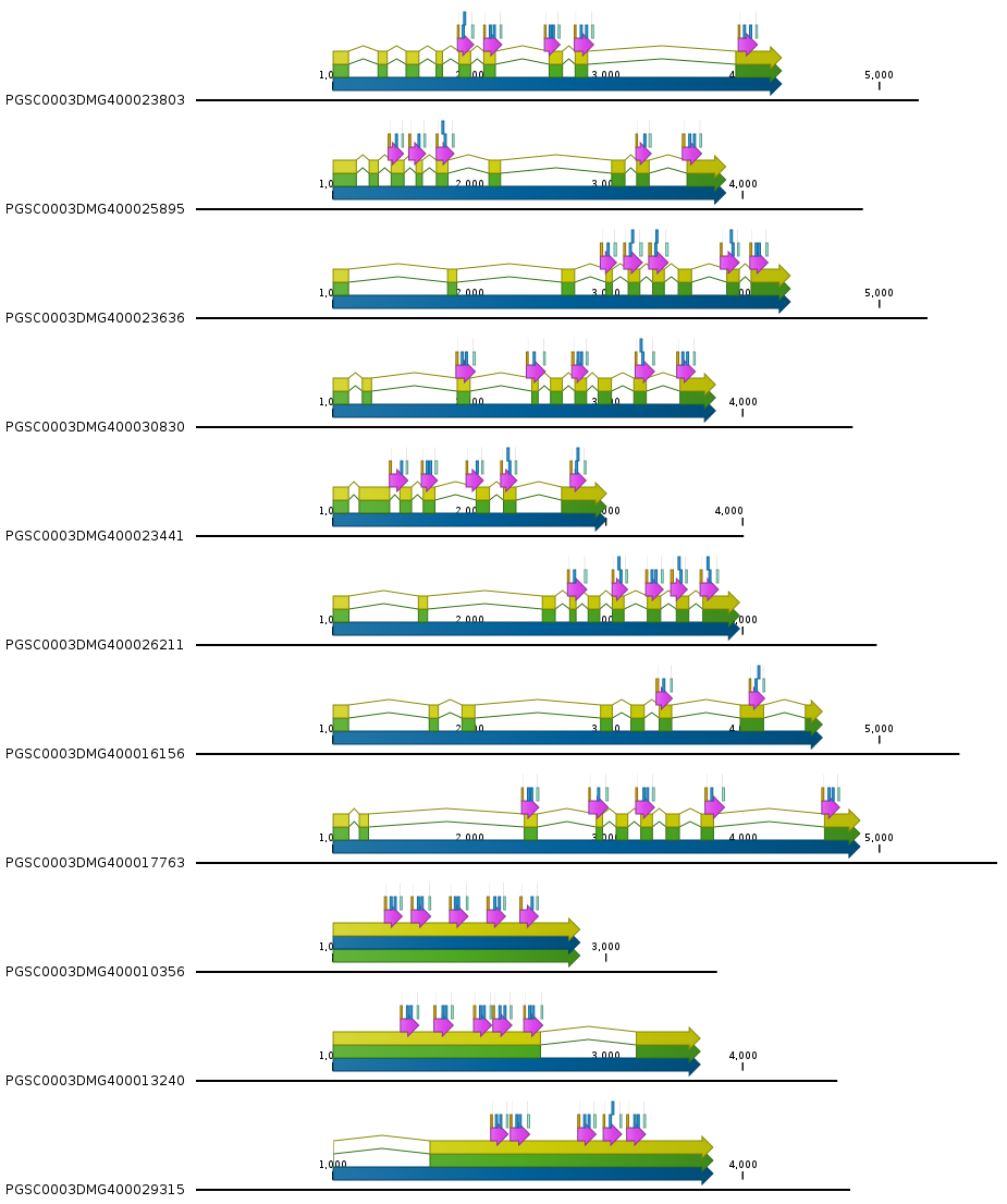
Optionally, SMAP design also provides:* a summary file (total number of amplicons designed by Primer3, total number of gRNAs designed, number of gRNAs after filtering).* a summary plot showing the number of amplicons and gRNAs that were designed per gene.* a SMAP (BED) file that is needed as input for downstream analysis with SMAP haplotype-sites.* a border (GFF) file that is needed as input for downstream analysis with SMAP haplotype-window.* a gRNA (FASTA) file that is needed as input for downstream analysis with SMAP haplotype-window.* a debug file (GFF file) containing all amplicons designed by Primer3 and all gRNAs from the input list before filtering.* ‘all-amplicons’ files (GFF file, a primer and gRNA file) containing all amplicons with their respective gRNAs (not just the non-overlapping amplicons in the output files).
Gene |
Total # amplicons |
Total # gRNAs |
Amps with gRNAs |
Amps with 2 gRNAs |
# gRNAs after TTTT filtering |
# gRNAs after restriction site filtering |
# gRNAs after intron filtering |
# gRNAs after complete filtering |
|---|---|---|---|---|---|---|---|---|
PGSC0003DMG400023803 |
150 |
394 |
24 |
10 |
307 |
305 |
78 |
45 |
PGSC0003DMG400025895 |
145 |
301 |
13 |
7 |
243 |
240 |
76 |
44 |
PGSC0003DMG400023636 |
128 |
284 |
9 |
6 |
230 |
230 |
46 |
27 |
PGSC0003DMG400030830 |
144 |
332 |
19 |
9 |
269 |
267 |
64 |
42 |
PGSC0003DMG400023441 |
150 |
292 |
11 |
7 |
268 |
265 |
58 |
31 |
PGSC0003DMG400026211 |
150 |
275 |
15 |
7 |
194 |
190 |
55 |
40 |
PGSC0003DMG400016156 |
127 |
297 |
5 |
2 |
229 |
226 |
40 |
30 |
PGSC0003DMG400017763 |
150 |
343 |
15 |
10 |
269 |
267 |
52 |
37 |
PGSC0003DMG400010356 |
150 |
255 |
54 |
38 |
220 |
220 |
128 |
75 |
PGSC0003DMG400013240 |
150 |
383 |
54 |
36 |
324 |
322 |
140 |
82 |
PGSC0003DMG400029315 |
143 |
353 |
71 |
50 |
303 |
302 |
144 |
92 |
average |
144.3 |
319 |
26.4 |
16.5 |
259.6 |
257.6 |
80.1 |
50 |
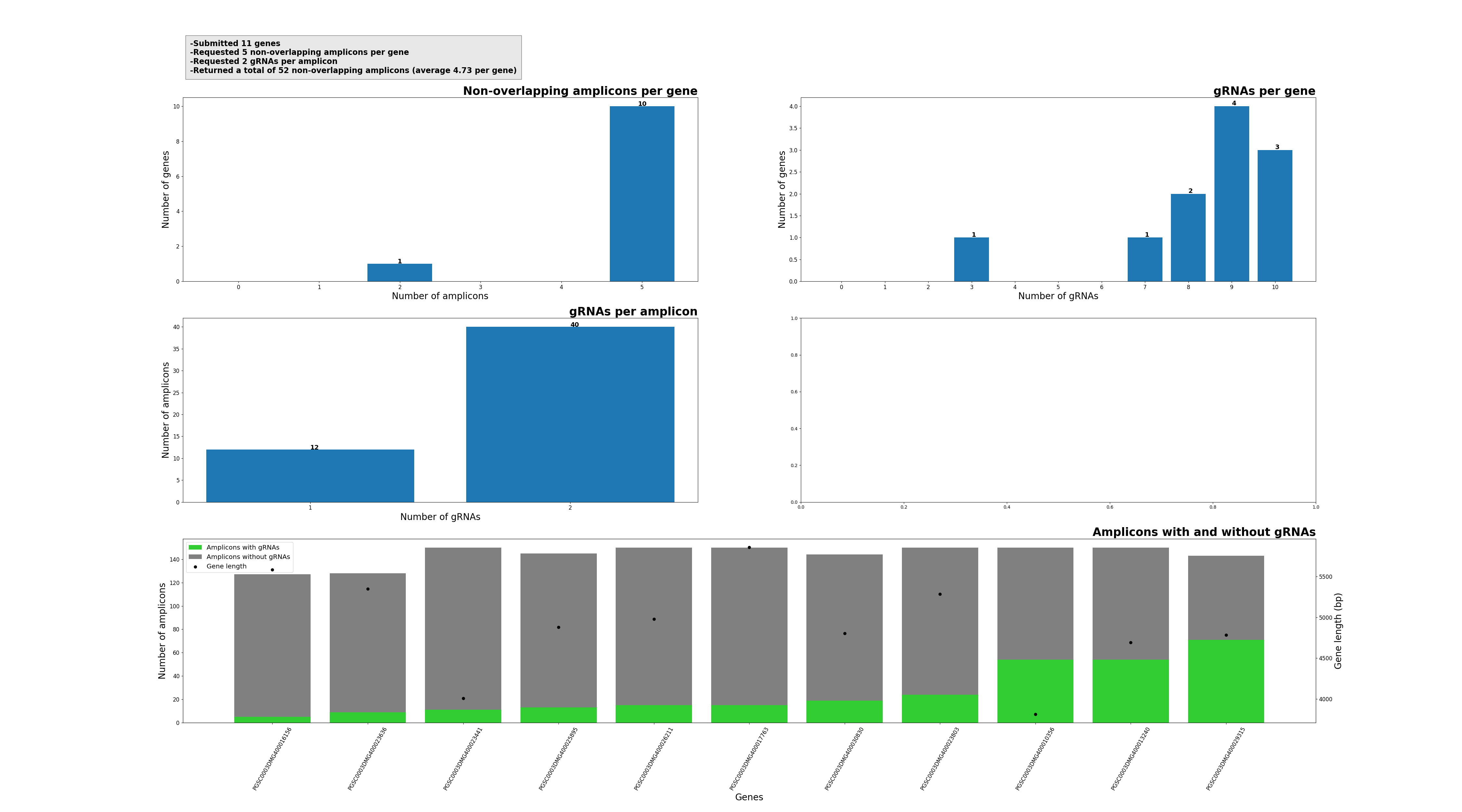
PGSC0003DMG400023803 |
1929 |
2013 |
PGSC0003DMG400023803:1930-2013_+ |
. |
+ |
1930,2013 |
. |
2 |
HiPlex_Set1_stu_all_selected_genes_extended_1000_bp_output |
PGSC0003DMG400023803 |
2121 |
2221 |
PGSC0003DMG400023803:2122-2221_+ |
. |
+ |
2122,2221 |
. |
2 |
HiPlex_Set1_stu_all_selected_genes_extended_1000_bp_output |
PGSC0003DMG400023803 |
2565 |
2645 |
PGSC0003DMG400023803:2566-2645_+ |
. |
+ |
2566,2645 |
. |
2 |
HiPlex_Set1_stu_all_selected_genes_extended_1000_bp_output |
PGSC0003DMG400023803 |
2784 |
2890 |
PGSC0003DMG400023803:2785-2890_+ |
. |
+ |
2785,2890 |
. |
2 |
HiPlex_Set1_stu_all_selected_genes_extended_1000_bp_output |
PGSC0003DMG400023803 |
3983 |
4091 |
PGSC0003DMG400023803:3984-4091_+ |
. |
+ |
3984,4091 |
. |
2 |
HiPlex_Set1_stu_all_selected_genes_extended_1000_bp_output |
PGSC0003DMG400025895 |
1426 |
1502 |
PGSC0003DMG400025895:1427-1502_+ |
. |
+ |
1427,1502 |
. |
2 |
HiPlex_Set1_stu_all_selected_genes_extended_1000_bp_output |
PGSC0003DMG400025895 |
1575 |
1663 |
PGSC0003DMG400025895:1576-1663_+ |
. |
+ |
1576,1663 |
. |
2 |
HiPlex_Set1_stu_all_selected_genes_extended_1000_bp_output |
PGSC0003DMG400025895 |
1774 |
1872 |
PGSC0003DMG400025895:1775-1872_+ |
. |
+ |
1775,1872 |
. |
2 |
HiPlex_Set1_stu_all_selected_genes_extended_1000_bp_output |
PGSC0003DMG400025895 |
3234 |
3310 |
PGSC0003DMG400025895:3235-3310_+ |
. |
+ |
3235,3310 |
. |
2 |
HiPlex_Set1_stu_all_selected_genes_extended_1000_bp_output |
PGSC0003DMG400025895 |
3580 |
3682 |
PGSC0003DMG400025895:3581-3682_+ |
. |
+ |
3581,3682 |
. |
2 |
HiPlex_Set1_stu_all_selected_genes_extended_1000_bp_output |
PGSC0003DMG400023636 |
2979 |
3054 |
PGSC0003DMG400023636:2980-3054_+ |
. |
+ |
2980,3054 |
. |
2 |
HiPlex_Set1_stu_all_selected_genes_extended_1000_bp_output |
PGSC0003DMG400023636 |
3147 |
3243 |
PGSC0003DMG400023636:3148-3243_+ |
. |
+ |
3148,3243 |
. |
2 |
HiPlex_Set1_stu_all_selected_genes_extended_1000_bp_output |
PGSC0003DMG400023636 |
3335 |
3433 |
PGSC0003DMG400023636:3336-3433_+ |
. |
+ |
3336,3433 |
. |
2 |
HiPlex_Set1_stu_all_selected_genes_extended_1000_bp_output |
PGSC0003DMG400023636 |
3852 |
3958 |
PGSC0003DMG400023636:3853-3958_+ |
. |
+ |
3853,3958 |
. |
2 |
HiPlex_Set1_stu_all_selected_genes_extended_1000_bp_output |
PGSC0003DMG400023636 |
4070 |
4165 |
PGSC0003DMG400023636:4071-4165_+ |
. |
+ |
4071,4165 |
. |
2 |
HiPlex_Set1_stu_all_selected_genes_extended_1000_bp_output |
PGSC0003DMG400030830 |
1922 |
2024 |
PGSC0003DMG400030830:1923-2024_+ |
. |
+ |
1923,2024 |
. |
2 |
HiPlex_Set1_stu_all_selected_genes_extended_1000_bp_output |
PGSC0003DMG400030830 |
2434 |
2539 |
PGSC0003DMG400030830:2435-2539_+ |
. |
+ |
2435,2539 |
. |
2 |
HiPlex_Set1_stu_all_selected_genes_extended_1000_bp_output |
PGSC0003DMG400030830 |
2769 |
2851 |
PGSC0003DMG400030830:2770-2851_+ |
. |
+ |
2770,2851 |
. |
2 |
HiPlex_Set1_stu_all_selected_genes_extended_1000_bp_output |
PGSC0003DMG400030830 |
3229 |
3338 |
PGSC0003DMG400030830:3230-3338_+ |
. |
+ |
3230,3338 |
. |
2 |
HiPlex_Set1_stu_all_selected_genes_extended_1000_bp_output |
PGSC0003DMG400030830 |
3536 |
3636 |
PGSC0003DMG400030830:3537-3636_+ |
. |
+ |
3537,3636 |
. |
2 |
HiPlex_Set1_stu_all_selected_genes_extended_1000_bp_output |
PGSC0003DMG400023441 |
1434 |
1534 |
PGSC0003DMG400023441:1435-1534_+ |
. |
+ |
1435,1534 |
. |
2 |
HiPlex_Set1_stu_all_selected_genes_extended_1000_bp_output |
PGSC0003DMG400023441 |
1666 |
1745 |
PGSC0003DMG400023441:1667-1745_+ |
. |
+ |
1667,1745 |
. |
2 |
HiPlex_Set1_stu_all_selected_genes_extended_1000_bp_output |
PGSC0003DMG400023441 |
1992 |
2086 |
PGSC0003DMG400023441:1993-2086_+ |
. |
+ |
1993,2086 |
. |
2 |
HiPlex_Set1_stu_all_selected_genes_extended_1000_bp_output |
PGSC0003DMG400023441 |
2246 |
2331 |
PGSC0003DMG400023441:2247-2331_+ |
. |
+ |
2247,2331 |
. |
2 |
HiPlex_Set1_stu_all_selected_genes_extended_1000_bp_output |
PGSC0003DMG400023441 |
2754 |
2837 |
PGSC0003DMG400023441:2755-2837_+ |
. |
+ |
2755,2837 |
. |
2 |
HiPlex_Set1_stu_all_selected_genes_extended_1000_bp_output |
PGSC0003DMG400026211 |
2735 |
2838 |
PGSC0003DMG400026211:2736-2838_+ |
. |
+ |
2736,2838 |
. |
2 |
HiPlex_Set1_stu_all_selected_genes_extended_1000_bp_output |
PGSC0003DMG400026211 |
3061 |
3140 |
PGSC0003DMG400026211:3062-3140_+ |
. |
+ |
3062,3140 |
. |
2 |
HiPlex_Set1_stu_all_selected_genes_extended_1000_bp_output |
PGSC0003DMG400026211 |
3308 |
3400 |
PGSC0003DMG400026211:3309-3400_+ |
. |
+ |
3309,3400 |
. |
2 |
HiPlex_Set1_stu_all_selected_genes_extended_1000_bp_output |
PGSC0003DMG400026211 |
3496 |
3578 |
PGSC0003DMG400026211:3497-3578_+ |
. |
+ |
3497,3578 |
. |
2 |
HiPlex_Set1_stu_all_selected_genes_extended_1000_bp_output |
PGSC0003DMG400026211 |
3707 |
3804 |
PGSC0003DMG400026211:3708-3804_+ |
. |
+ |
3708,3804 |
. |
2 |
HiPlex_Set1_stu_all_selected_genes_extended_1000_bp_output |
PGSC0003DMG400016156 |
3388 |
3468 |
PGSC0003DMG400016156:3389-3468_+ |
. |
+ |
3389,3468 |
. |
2 |
HiPlex_Set1_stu_all_selected_genes_extended_1000_bp_output |
PGSC0003DMG400016156 |
4063 |
4144 |
PGSC0003DMG400016156:4064-4144_+ |
. |
+ |
4064,4144 |
. |
2 |
HiPlex_Set1_stu_all_selected_genes_extended_1000_bp_output |
PGSC0003DMG400017763 |
2398 |
2488 |
PGSC0003DMG400017763:2399-2488_+ |
. |
+ |
2399,2488 |
. |
2 |
HiPlex_Set1_stu_all_selected_genes_extended_1000_bp_output |
PGSC0003DMG400017763 |
2888 |
2996 |
PGSC0003DMG400017763:2889-2996_+ |
. |
+ |
2889,2996 |
. |
2 |
HiPlex_Set1_stu_all_selected_genes_extended_1000_bp_output |
PGSC0003DMG400017763 |
3234 |
3335 |
PGSC0003DMG400017763:3235-3335_+ |
. |
+ |
3235,3335 |
. |
2 |
HiPlex_Set1_stu_all_selected_genes_extended_1000_bp_output |
PGSC0003DMG400017763 |
3744 |
3847 |
PGSC0003DMG400017763:3745-3847_+ |
. |
+ |
3745,3847 |
. |
2 |
HiPlex_Set1_stu_all_selected_genes_extended_1000_bp_output |
PGSC0003DMG400017763 |
4597 |
4692 |
PGSC0003DMG400017763:4598-4692_+ |
. |
+ |
4598,4692 |
. |
2 |
HiPlex_Set1_stu_all_selected_genes_extended_1000_bp_output |
PGSC0003DMG400010356 |
1398 |
1490 |
PGSC0003DMG400010356:1399-1490_+ |
. |
+ |
1399,1490 |
. |
2 |
HiPlex_Set1_stu_all_selected_genes_extended_1000_bp_output |
PGSC0003DMG400010356 |
1591 |
1700 |
PGSC0003DMG400010356:1592-1700_+ |
. |
+ |
1592,1700 |
. |
2 |
HiPlex_Set1_stu_all_selected_genes_extended_1000_bp_output |
PGSC0003DMG400010356 |
1871 |
1974 |
PGSC0003DMG400010356:1872-1974_+ |
. |
+ |
1872,1974 |
. |
2 |
HiPlex_Set1_stu_all_selected_genes_extended_1000_bp_output |
PGSC0003DMG400010356 |
2148 |
2247 |
PGSC0003DMG400010356:2149-2247_+ |
. |
+ |
2149,2247 |
. |
2 |
HiPlex_Set1_stu_all_selected_genes_extended_1000_bp_output |
PGSC0003DMG400010356 |
2390 |
2488 |
PGSC0003DMG400010356:2391-2488_+ |
. |
+ |
2391,2488 |
. |
2 |
HiPlex_Set1_stu_all_selected_genes_extended_1000_bp_output |
PGSC0003DMG400013240 |
1512 |
1614 |
PGSC0003DMG400013240:1513-1614_+ |
. |
+ |
1513,1614 |
. |
2 |
HiPlex_Set1_stu_all_selected_genes_extended_1000_bp_output |
PGSC0003DMG400013240 |
1759 |
1864 |
PGSC0003DMG400013240:1760-1864_+ |
. |
+ |
1760,1864 |
. |
2 |
HiPlex_Set1_stu_all_selected_genes_extended_1000_bp_output |
PGSC0003DMG400013240 |
2050 |
2147 |
PGSC0003DMG400013240:2051-2147_+ |
. |
+ |
2051,2147 |
. |
2 |
HiPlex_Set1_stu_all_selected_genes_extended_1000_bp_output |
PGSC0003DMG400013240 |
2188 |
2295 |
PGSC0003DMG400013240:2189-2295_+ |
. |
+ |
2189,2295 |
. |
2 |
HiPlex_Set1_stu_all_selected_genes_extended_1000_bp_output |
PGSC0003DMG400013240 |
2414 |
2521 |
PGSC0003DMG400013240:2415-2521_+ |
. |
+ |
2415,2521 |
. |
2 |
HiPlex_Set1_stu_all_selected_genes_extended_1000_bp_output |
PGSC0003DMG400029315 |
2172 |
2267 |
PGSC0003DMG400029315:2173-2267_+ |
. |
+ |
2173,2267 |
. |
2 |
HiPlex_Set1_stu_all_selected_genes_extended_1000_bp_output |
PGSC0003DMG400029315 |
2315 |
2421 |
PGSC0003DMG400029315:2316-2421_+ |
. |
+ |
2316,2421 |
. |
2 |
HiPlex_Set1_stu_all_selected_genes_extended_1000_bp_output |
PGSC0003DMG400029315 |
2812 |
2906 |
PGSC0003DMG400029315:2813-2906_+ |
. |
+ |
2813,2906 |
. |
2 |
HiPlex_Set1_stu_all_selected_genes_extended_1000_bp_output |
PGSC0003DMG400029315 |
2995 |
3098 |
PGSC0003DMG400029315:2996-3098_+ |
. |
+ |
2996,3098 |
. |
2 |
HiPlex_Set1_stu_all_selected_genes_extended_1000_bp_output |
PGSC0003DMG400029315 |
3169 |
3271 |
PGSC0003DMG400029315:3170-3271_+ |
. |
+ |
3170,3271 |
. |
2 |
HiPlex_Set1_stu_all_selected_genes_extended_1000_bp_output |
PGSC0003DMG400023803 |
Primer3 |
border_up |
1920 |
1929 |
. |
+ |
. |
NAME=PGSC0003DMG400023803_Amplicon01 |
PGSC0003DMG400023803 |
Primer3 |
border_down |
2014 |
2023 |
. |
+ |
. |
NAME=PGSC0003DMG400023803_Amplicon01 |
PGSC0003DMG400023803 |
Primer3 |
border_up |
2112 |
2121 |
. |
+ |
. |
NAME=PGSC0003DMG400023803_Amplicon02 |
PGSC0003DMG400023803 |
Primer3 |
border_down |
2222 |
2231 |
. |
+ |
. |
NAME=PGSC0003DMG400023803_Amplicon02 |
PGSC0003DMG400023803 |
Primer3 |
border_up |
2556 |
2565 |
. |
+ |
. |
NAME=PGSC0003DMG400023803_Amplicon03 |
PGSC0003DMG400023803 |
Primer3 |
border_down |
2646 |
2655 |
. |
+ |
. |
NAME=PGSC0003DMG400023803_Amplicon03 |
PGSC0003DMG400023803 |
Primer3 |
border_up |
2775 |
2784 |
. |
+ |
. |
NAME=PGSC0003DMG400023803_Amplicon04 |
PGSC0003DMG400023803 |
Primer3 |
border_down |
2891 |
2900 |
. |
+ |
. |
NAME=PGSC0003DMG400023803_Amplicon04 |
PGSC0003DMG400023803 |
Primer3 |
border_up |
3974 |
3983 |
. |
+ |
. |
NAME=PGSC0003DMG400023803_Amplicon05 |
PGSC0003DMG400023803 |
Primer3 |
border_down |
4092 |
4101 |
. |
+ |
. |
NAME=PGSC0003DMG400023803_Amplicon05 |
PGSC0003DMG400025895 |
Primer3 |
border_up |
1417 |
1426 |
. |
+ |
. |
NAME=PGSC0003DMG400025895_Amplicon01 |
PGSC0003DMG400025895 |
Primer3 |
border_down |
1503 |
1512 |
. |
+ |
. |
NAME=PGSC0003DMG400025895_Amplicon01 |
PGSC0003DMG400025895 |
Primer3 |
border_up |
1566 |
1575 |
. |
+ |
. |
NAME=PGSC0003DMG400025895_Amplicon02 |
PGSC0003DMG400025895 |
Primer3 |
border_down |
1664 |
1673 |
. |
+ |
. |
NAME=PGSC0003DMG400025895_Amplicon02 |
PGSC0003DMG400025895 |
Primer3 |
border_up |
1765 |
1774 |
. |
+ |
. |
NAME=PGSC0003DMG400025895_Amplicon03 |
PGSC0003DMG400025895 |
Primer3 |
border_down |
1873 |
1882 |
. |
+ |
. |
NAME=PGSC0003DMG400025895_Amplicon03 |
PGSC0003DMG400025895 |
Primer3 |
border_up |
3225 |
3234 |
. |
+ |
. |
NAME=PGSC0003DMG400025895_Amplicon04 |
PGSC0003DMG400025895 |
Primer3 |
border_down |
3311 |
3320 |
. |
+ |
. |
NAME=PGSC0003DMG400025895_Amplicon04 |
PGSC0003DMG400025895 |
Primer3 |
border_up |
3571 |
3580 |
. |
+ |
. |
NAME=PGSC0003DMG400025895_Amplicon05 |
PGSC0003DMG400025895 |
Primer3 |
border_down |
3683 |
3692 |
. |
+ |
. |
NAME=PGSC0003DMG400025895_Amplicon05 |
PGSC0003DMG400023636 |
Primer3 |
border_up |
2970 |
2979 |
. |
+ |
. |
NAME=PGSC0003DMG400023636_Amplicon01 |
PGSC0003DMG400023636 |
Primer3 |
border_down |
3055 |
3064 |
. |
+ |
. |
NAME=PGSC0003DMG400023636_Amplicon01 |
PGSC0003DMG400023636 |
Primer3 |
border_up |
3138 |
3147 |
. |
+ |
. |
NAME=PGSC0003DMG400023636_Amplicon02 |
PGSC0003DMG400023636 |
Primer3 |
border_down |
3244 |
3253 |
. |
+ |
. |
NAME=PGSC0003DMG400023636_Amplicon02 |
PGSC0003DMG400023636 |
Primer3 |
border_up |
3326 |
3335 |
. |
+ |
. |
NAME=PGSC0003DMG400023636_Amplicon03 |
PGSC0003DMG400023636 |
Primer3 |
border_down |
3434 |
3443 |
. |
+ |
. |
NAME=PGSC0003DMG400023636_Amplicon03 |
PGSC0003DMG400023636 |
Primer3 |
border_up |
3843 |
3852 |
. |
+ |
. |
NAME=PGSC0003DMG400023636_Amplicon04 |
PGSC0003DMG400023636 |
Primer3 |
border_down |
3959 |
3968 |
. |
+ |
. |
NAME=PGSC0003DMG400023636_Amplicon04 |
PGSC0003DMG400023636 |
Primer3 |
border_up |
4061 |
4070 |
. |
+ |
. |
NAME=PGSC0003DMG400023636_Amplicon05 |
PGSC0003DMG400023636 |
Primer3 |
border_down |
4166 |
4175 |
. |
+ |
. |
NAME=PGSC0003DMG400023636_Amplicon05 |
PGSC0003DMG400030830 |
Primer3 |
border_up |
1913 |
1922 |
. |
+ |
. |
NAME=PGSC0003DMG400030830_Amplicon01 |
PGSC0003DMG400030830 |
Primer3 |
border_down |
2025 |
2034 |
. |
+ |
. |
NAME=PGSC0003DMG400030830_Amplicon01 |
PGSC0003DMG400030830 |
Primer3 |
border_up |
2425 |
2434 |
. |
+ |
. |
NAME=PGSC0003DMG400030830_Amplicon02 |
PGSC0003DMG400030830 |
Primer3 |
border_down |
2540 |
2549 |
. |
+ |
. |
NAME=PGSC0003DMG400030830_Amplicon02 |
PGSC0003DMG400030830 |
Primer3 |
border_up |
2760 |
2769 |
. |
+ |
. |
NAME=PGSC0003DMG400030830_Amplicon03 |
PGSC0003DMG400030830 |
Primer3 |
border_down |
2852 |
2861 |
. |
+ |
. |
NAME=PGSC0003DMG400030830_Amplicon03 |
PGSC0003DMG400030830 |
Primer3 |
border_up |
3220 |
3229 |
. |
+ |
. |
NAME=PGSC0003DMG400030830_Amplicon04 |
PGSC0003DMG400030830 |
Primer3 |
border_down |
3339 |
3348 |
. |
+ |
. |
NAME=PGSC0003DMG400030830_Amplicon04 |
PGSC0003DMG400030830 |
Primer3 |
border_up |
3527 |
3536 |
. |
+ |
. |
NAME=PGSC0003DMG400030830_Amplicon05 |
PGSC0003DMG400030830 |
Primer3 |
border_down |
3637 |
3646 |
. |
+ |
. |
NAME=PGSC0003DMG400030830_Amplicon05 |
PGSC0003DMG400023441 |
Primer3 |
border_up |
1425 |
1434 |
. |
+ |
. |
NAME=PGSC0003DMG400023441_Amplicon01 |
PGSC0003DMG400023441 |
Primer3 |
border_down |
1535 |
1544 |
. |
+ |
. |
NAME=PGSC0003DMG400023441_Amplicon01 |
PGSC0003DMG400023441 |
Primer3 |
border_up |
1657 |
1666 |
. |
+ |
. |
NAME=PGSC0003DMG400023441_Amplicon02 |
PGSC0003DMG400023441 |
Primer3 |
border_down |
1746 |
1755 |
. |
+ |
. |
NAME=PGSC0003DMG400023441_Amplicon02 |
PGSC0003DMG400023441 |
Primer3 |
border_up |
1983 |
1992 |
. |
+ |
. |
NAME=PGSC0003DMG400023441_Amplicon03 |
PGSC0003DMG400023441 |
Primer3 |
border_down |
2087 |
2096 |
. |
+ |
. |
NAME=PGSC0003DMG400023441_Amplicon03 |
PGSC0003DMG400023441 |
Primer3 |
border_up |
2237 |
2246 |
. |
+ |
. |
NAME=PGSC0003DMG400023441_Amplicon04 |
PGSC0003DMG400023441 |
Primer3 |
border_down |
2332 |
2341 |
. |
+ |
. |
NAME=PGSC0003DMG400023441_Amplicon04 |
PGSC0003DMG400023441 |
Primer3 |
border_up |
2745 |
2754 |
. |
+ |
. |
NAME=PGSC0003DMG400023441_Amplicon05 |
PGSC0003DMG400023441 |
Primer3 |
border_down |
2838 |
2847 |
. |
+ |
. |
NAME=PGSC0003DMG400023441_Amplicon05 |
PGSC0003DMG400026211 |
Primer3 |
border_up |
2726 |
2735 |
. |
+ |
. |
NAME=PGSC0003DMG400026211_Amplicon01 |
PGSC0003DMG400026211 |
Primer3 |
border_down |
2839 |
2848 |
. |
+ |
. |
NAME=PGSC0003DMG400026211_Amplicon01 |
PGSC0003DMG400026211 |
Primer3 |
border_up |
3052 |
3061 |
. |
+ |
. |
NAME=PGSC0003DMG400026211_Amplicon02 |
PGSC0003DMG400026211 |
Primer3 |
border_down |
3141 |
3150 |
. |
+ |
. |
NAME=PGSC0003DMG400026211_Amplicon02 |
PGSC0003DMG400026211 |
Primer3 |
border_up |
3299 |
3308 |
. |
+ |
. |
NAME=PGSC0003DMG400026211_Amplicon03 |
PGSC0003DMG400026211 |
Primer3 |
border_down |
3401 |
3410 |
. |
+ |
. |
NAME=PGSC0003DMG400026211_Amplicon03 |
PGSC0003DMG400026211 |
Primer3 |
border_up |
3487 |
3496 |
. |
+ |
. |
NAME=PGSC0003DMG400026211_Amplicon04 |
PGSC0003DMG400026211 |
Primer3 |
border_down |
3579 |
3588 |
. |
+ |
. |
NAME=PGSC0003DMG400026211_Amplicon04 |
PGSC0003DMG400026211 |
Primer3 |
border_up |
3698 |
3707 |
. |
+ |
. |
NAME=PGSC0003DMG400026211_Amplicon05 |
PGSC0003DMG400026211 |
Primer3 |
border_down |
3805 |
3814 |
. |
+ |
. |
NAME=PGSC0003DMG400026211_Amplicon05 |
PGSC0003DMG400016156 |
Primer3 |
border_up |
3379 |
3388 |
. |
+ |
. |
NAME=PGSC0003DMG400016156_Amplicon01 |
PGSC0003DMG400016156 |
Primer3 |
border_down |
3469 |
3478 |
. |
+ |
. |
NAME=PGSC0003DMG400016156_Amplicon01 |
PGSC0003DMG400016156 |
Primer3 |
border_up |
4054 |
4063 |
. |
+ |
. |
NAME=PGSC0003DMG400016156_Amplicon02 |
PGSC0003DMG400016156 |
Primer3 |
border_down |
4145 |
4154 |
. |
+ |
. |
NAME=PGSC0003DMG400016156_Amplicon02 |
PGSC0003DMG400017763 |
Primer3 |
border_up |
2389 |
2398 |
. |
+ |
. |
NAME=PGSC0003DMG400017763_Amplicon01 |
PGSC0003DMG400017763 |
Primer3 |
border_down |
2489 |
2498 |
. |
+ |
. |
NAME=PGSC0003DMG400017763_Amplicon01 |
PGSC0003DMG400017763 |
Primer3 |
border_up |
2879 |
2888 |
. |
+ |
. |
NAME=PGSC0003DMG400017763_Amplicon02 |
PGSC0003DMG400017763 |
Primer3 |
border_down |
2997 |
3006 |
. |
+ |
. |
NAME=PGSC0003DMG400017763_Amplicon02 |
PGSC0003DMG400017763 |
Primer3 |
border_up |
3225 |
3234 |
. |
+ |
. |
NAME=PGSC0003DMG400017763_Amplicon03 |
PGSC0003DMG400017763 |
Primer3 |
border_down |
3336 |
3345 |
. |
+ |
. |
NAME=PGSC0003DMG400017763_Amplicon03 |
PGSC0003DMG400017763 |
Primer3 |
border_up |
3735 |
3744 |
. |
+ |
. |
NAME=PGSC0003DMG400017763_Amplicon04 |
PGSC0003DMG400017763 |
Primer3 |
border_down |
3848 |
3857 |
. |
+ |
. |
NAME=PGSC0003DMG400017763_Amplicon04 |
PGSC0003DMG400017763 |
Primer3 |
border_up |
4588 |
4597 |
. |
+ |
. |
NAME=PGSC0003DMG400017763_Amplicon05 |
PGSC0003DMG400017763 |
Primer3 |
border_down |
4693 |
4702 |
. |
+ |
. |
NAME=PGSC0003DMG400017763_Amplicon05 |
PGSC0003DMG400010356 |
Primer3 |
border_up |
1389 |
1398 |
. |
+ |
. |
NAME=PGSC0003DMG400010356_Amplicon01 |
PGSC0003DMG400010356 |
Primer3 |
border_down |
1491 |
1500 |
. |
+ |
. |
NAME=PGSC0003DMG400010356_Amplicon01 |
PGSC0003DMG400010356 |
Primer3 |
border_up |
1582 |
1591 |
. |
+ |
. |
NAME=PGSC0003DMG400010356_Amplicon02 |
PGSC0003DMG400010356 |
Primer3 |
border_down |
1701 |
1710 |
. |
+ |
. |
NAME=PGSC0003DMG400010356_Amplicon02 |
PGSC0003DMG400010356 |
Primer3 |
border_up |
1862 |
1871 |
. |
+ |
. |
NAME=PGSC0003DMG400010356_Amplicon03 |
PGSC0003DMG400010356 |
Primer3 |
border_down |
1975 |
1984 |
. |
+ |
. |
NAME=PGSC0003DMG400010356_Amplicon03 |
PGSC0003DMG400010356 |
Primer3 |
border_up |
2139 |
2148 |
. |
+ |
. |
NAME=PGSC0003DMG400010356_Amplicon04 |
PGSC0003DMG400010356 |
Primer3 |
border_down |
2248 |
2257 |
. |
+ |
. |
NAME=PGSC0003DMG400010356_Amplicon04 |
PGSC0003DMG400010356 |
Primer3 |
border_up |
2381 |
2390 |
. |
+ |
. |
NAME=PGSC0003DMG400010356_Amplicon05 |
PGSC0003DMG400010356 |
Primer3 |
border_down |
2489 |
2498 |
. |
+ |
. |
NAME=PGSC0003DMG400010356_Amplicon05 |
PGSC0003DMG400013240 |
Primer3 |
border_up |
1503 |
1512 |
. |
+ |
. |
NAME=PGSC0003DMG400013240_Amplicon01 |
PGSC0003DMG400013240 |
Primer3 |
border_down |
1615 |
1624 |
. |
+ |
. |
NAME=PGSC0003DMG400013240_Amplicon01 |
PGSC0003DMG400013240 |
Primer3 |
border_up |
1750 |
1759 |
. |
+ |
. |
NAME=PGSC0003DMG400013240_Amplicon02 |
PGSC0003DMG400013240 |
Primer3 |
border_down |
1865 |
1874 |
. |
+ |
. |
NAME=PGSC0003DMG400013240_Amplicon02 |
PGSC0003DMG400013240 |
Primer3 |
border_up |
2041 |
2050 |
. |
+ |
. |
NAME=PGSC0003DMG400013240_Amplicon03 |
PGSC0003DMG400013240 |
Primer3 |
border_down |
2148 |
2157 |
. |
+ |
. |
NAME=PGSC0003DMG400013240_Amplicon03 |
PGSC0003DMG400013240 |
Primer3 |
border_up |
2179 |
2188 |
. |
+ |
. |
NAME=PGSC0003DMG400013240_Amplicon04 |
PGSC0003DMG400013240 |
Primer3 |
border_down |
2296 |
2305 |
. |
+ |
. |
NAME=PGSC0003DMG400013240_Amplicon04 |
PGSC0003DMG400013240 |
Primer3 |
border_up |
2405 |
2414 |
. |
+ |
. |
NAME=PGSC0003DMG400013240_Amplicon05 |
PGSC0003DMG400013240 |
Primer3 |
border_down |
2522 |
2531 |
. |
+ |
. |
NAME=PGSC0003DMG400013240_Amplicon05 |
PGSC0003DMG400029315 |
Primer3 |
border_up |
2163 |
2172 |
. |
+ |
. |
NAME=PGSC0003DMG400029315_Amplicon01 |
PGSC0003DMG400029315 |
Primer3 |
border_down |
2268 |
2277 |
. |
+ |
. |
NAME=PGSC0003DMG400029315_Amplicon01 |
PGSC0003DMG400029315 |
Primer3 |
border_up |
2306 |
2315 |
. |
+ |
. |
NAME=PGSC0003DMG400029315_Amplicon02 |
PGSC0003DMG400029315 |
Primer3 |
border_down |
2422 |
2431 |
. |
+ |
. |
NAME=PGSC0003DMG400029315_Amplicon02 |
PGSC0003DMG400029315 |
Primer3 |
border_up |
2803 |
2812 |
. |
+ |
. |
NAME=PGSC0003DMG400029315_Amplicon03 |
PGSC0003DMG400029315 |
Primer3 |
border_down |
2907 |
2916 |
. |
+ |
. |
NAME=PGSC0003DMG400029315_Amplicon03 |
PGSC0003DMG400029315 |
Primer3 |
border_up |
2986 |
2995 |
. |
+ |
. |
NAME=PGSC0003DMG400029315_Amplicon04 |
PGSC0003DMG400029315 |
Primer3 |
border_down |
3099 |
3108 |
. |
+ |
. |
NAME=PGSC0003DMG400029315_Amplicon04 |
PGSC0003DMG400029315 |
Primer3 |
border_up |
3160 |
3169 |
. |
+ |
. |
NAME=PGSC0003DMG400029315_Amplicon05 |
PGSC0003DMG400029315 |
Primer3 |
border_down |
3272 |
3281 |
. |
+ |
. |
NAME=PGSC0003DMG400029315_Amplicon05 |
>PGSC0003DMG400023803_Amplicon01:gRNA01 |
AGCTGCACTTCCATCAAGAAGGG |
>PGSC0003DMG400023803_Amplicon01:gRNA02 |
CTGGAGAATACCCTTCTTGATGG |
>PGSC0003DMG400023803_Amplicon02:gRNA01 |
CTTGCCATCATATTCCCTTCTGG |
>PGSC0003DMG400023803_Amplicon02:gRNA02 |
TCCAGCTTATATTGCTCCAGAGG |
>PGSC0003DMG400023803_Amplicon03:gRNA01 |
AGTGACACTTTACGTGATGCTGG |
>PGSC0003DMG400023803_Amplicon03:gRNA02 |
CTGGCTGATGTCTGGTCATGTGG |
>PGSC0003DMG400023803_Amplicon04:gRNA01 |
TATTTGTTGCCAATTCCGCAAGG |
>PGSC0003DMG400023803_Amplicon04:gRNA02 |
TTCACATATCGCAAGATTGTAGG |
>PGSC0003DMG400023803_Amplicon05:gRNA01 |
GGAGTTGACAGAAGCAGCACAGG |
>PGSC0003DMG400023803_Amplicon05:gRNA02 |
CACTCTGAAGCGAAAATGTCGGG |
>PGSC0003DMG400025895_Amplicon01:gRNA01 |
TGATGGAATTTGCATCTGGAGGG |
>PGSC0003DMG400025895_Amplicon02:gRNA01 |
TGACCCCTGATATGAGTTGTTGG |
>PGSC0003DMG400025895_Amplicon03:gRNA01 |
TGGATGGTAGTCCTGCACCAAGG |
>PGSC0003DMG400025895_Amplicon03:gRNA02 |
AAATCACAAATCTTTAGCCTTGG |
>PGSC0003DMG400025895_Amplicon04:gRNA01 |
AATGTCGTCATCTAATATCAAGG |
>PGSC0003DMG400025895_Amplicon05:gRNA01 |
TATCCATGAGATCTGCAGGTAGG |
>PGSC0003DMG400025895_Amplicon05:gRNA02 |
CCGAGATCAAGAACCATGAGTGG |
>PGSC0003DMG400023636_Amplicon01:gRNA01 |
TTCTTTCAACAACTTATATCAGG |
>PGSC0003DMG400023636_Amplicon02:gRNA01 |
TTTCAAGCTTAAGATCTCTGTGG |
>PGSC0003DMG400023636_Amplicon02:gRNA02 |
TTGAAAACACATTGTTAGACGGG |
>PGSC0003DMG400023636_Amplicon03:gRNA01 |
TCACAACCAAAATCTACAGTTGG |
>PGSC0003DMG400023636_Amplicon03:gRNA02 |
AAAATCTACAGTTGGAACTCCGG |
>PGSC0003DMG400023636_Amplicon04:gRNA01 |
TGGACACTCGGACATAGTAAGGG |
>PGSC0003DMG400023636_Amplicon04:gRNA02 |
GATTACACTCCTTGGACACTCGG |
>PGSC0003DMG400023636_Amplicon05:gRNA01 |
TAAAGAATTTATGAAAGGAGAGG |
>PGSC0003DMG400023636_Amplicon05:gRNA02 |
GGCAAGTTCTTTAAGAACCATGG |
>PGSC0003DMG400030830_Amplicon01:gRNA01 |
TTTGCGAGGATCTGTAATGCTGG |
>PGSC0003DMG400030830_Amplicon01:gRNA02 |
GTAATGGAGTATGCTGCGGGAGG |
>PGSC0003DMG400030830_Amplicon02:gRNA01 |
TCTTTCAACAATTGATATCAGGG |
>PGSC0003DMG400030830_Amplicon03:gRNA01 |
ACCTGCTTATGTAGCACCAGAGG |
>PGSC0003DMG400030830_Amplicon03:gRNA02 |
CTCAACCTAAGTCCACTGTGGGG |
>PGSC0003DMG400030830_Amplicon04:gRNA01 |
TATGAGATGGCGGCATTCAAGGG |
>PGSC0003DMG400030830_Amplicon04:gRNA02 |
CAAAAATCCTGGCTATGAGATGG |
>PGSC0003DMG400030830_Amplicon05:gRNA01 |
TTACCAGTGGAACTGATGGAAGG |
>PGSC0003DMG400030830_Amplicon05:gRNA02 |
CAGAAATAAAAATGCATCCCTGG |
>PGSC0003DMG400023441_Amplicon01:gRNA01 |
CTGTCACAGAGATCTGAAATTGG |
>PGSC0003DMG400023441_Amplicon02:gRNA01 |
TAGAACCTCGGGTGCAATATAGG |
>PGSC0003DMG400023441_Amplicon02:gRNA02 |
TGGTGTTCCAACAGTCGACTTGG |
>PGSC0003DMG400023441_Amplicon03:gRNA01 |
TCTGCAGATGTATGGTCATGTGG |
>PGSC0003DMG400023441_Amplicon04:gRNA01 |
GTTTGCAATCATGAGATATATGG |
>PGSC0003DMG400023441_Amplicon04:gRNA02 |
GAGATATATGGACGTAGTCTGGG |
>PGSC0003DMG400023441_Amplicon05:gRNA01 |
GATCTCCTCAATGCTCTGAAGGG |
>PGSC0003DMG400023441_Amplicon05:gRNA02 |
ATGCTCTGAAGGGAGAATGTTGG |
>PGSC0003DMG400026211_Amplicon01:gRNA01 |
GGTATGACAGTAGCTGACACCGG |
>PGSC0003DMG400026211_Amplicon02:gRNA01 |
CTTTCGTGACAGGACCTCGGGGG |
>PGSC0003DMG400026211_Amplicon02:gRNA02 |
TCCTGCTTACATTGCCCCCGAGG |
>PGSC0003DMG400026211_Amplicon03:gRNA01 |
GATCTTCAGGATCCTCAAAAGGG |
>PGSC0003DMG400026211_Amplicon03:gRNA02 |
ACACTATATGTAATGTTAGTAGG |
>PGSC0003DMG400026211_Amplicon04:gRNA01 |
GGTGTGATTCGTACATAGTCGGG |
>PGSC0003DMG400026211_Amplicon04:gRNA02 |
ATAGTCGGGTATGGAGTGTTGGG |
>PGSC0003DMG400026211_Amplicon05:gRNA01 |
GAATCTGCCAAAAGAGCTGATGG |
>PGSC0003DMG400026211_Amplicon05:gRNA02 |
GGCAGATTCTTTAAGAACCAAGG |
>PGSC0003DMG400016156_Amplicon01:gRNA01 |
TTGAAACTCGAACGTAATAAGGG |
>PGSC0003DMG400016156_Amplicon02:gRNA01 |
ACTTCATCAATACTTTGAGTTGG |
>PGSC0003DMG400016156_Amplicon02:gRNA02 |
AGTGTTAGCTATAATTCAAGAGG |
>PGSC0003DMG400017763_Amplicon01:gRNA01 |
AGCAATAGTAATGGAGTATGCGG |
>PGSC0003DMG400017763_Amplicon01:gRNA02 |
CAGGAGGAGAACTCTTTCAGAGG |
>PGSC0003DMG400017763_Amplicon02:gRNA01 |
TCTTTCAACAATTGATATCAGGG |
>PGSC0003DMG400017763_Amplicon03:gRNA01 |
ATCTCCGGTGCAACGTAAGCTGG |
>PGSC0003DMG400017763_Amplicon03:gRNA02 |
CTCAACCAAAGTCCACTGTAGGG |
>PGSC0003DMG400017763_Amplicon04:gRNA01 |
CAGGGTCTGCTACAAAAATCCGG |
>PGSC0003DMG400017763_Amplicon05:gRNA01 |
TCGAATTCATGGAAGAAGGACGG |
>PGSC0003DMG400017763_Amplicon05:gRNA02 |
AGTTCTTCAAAAACCAAGGATGG |
>PGSC0003DMG400010356_Amplicon01:gRNA01 |
ACTTGCATATACAATATTCAGGG |
>PGSC0003DMG400010356_Amplicon01:gRNA02 |
AGGAGAGCTGGATGATGTGGAGG |
>PGSC0003DMG400010356_Amplicon02:gRNA01 |
ACTCAGCTCGATCTGTCTATTGG |
>PGSC0003DMG400010356_Amplicon02:gRNA02 |
AAAACTTTCATGGAAAATTTGGG |
>PGSC0003DMG400010356_Amplicon03:gRNA01 |
TCAAAGCTTTAAAGTGGCCACGG |
>PGSC0003DMG400010356_Amplicon03:gRNA02 |
CTCCAACACCATAGAGCACGTGG |
>PGSC0003DMG400010356_Amplicon04:gRNA01 |
TGTCAAGCTCCTTCGACACAGGG |
>PGSC0003DMG400010356_Amplicon04:gRNA02 |
TCACAATGTGCCATACTATGAGG |
>PGSC0003DMG400010356_Amplicon05:gRNA01 |
TCTCTTGGCAAGCTTCTTGTTGG |
>PGSC0003DMG400013240_Amplicon01:gRNA01 |
CCAAAATGCCAAGGCCACCGGGG |
>PGSC0003DMG400013240_Amplicon01:gRNA02 |
TTTCCTTGAAAATGGATCTACGG |
>PGSC0003DMG400013240_Amplicon02:gRNA01 |
ATTAGAGGTGGGCGTTGGCGCGG |
>PGSC0003DMG400013240_Amplicon02:gRNA02 |
GGTCGTACGAAGATTGCTACAGG |
>PGSC0003DMG400013240_Amplicon03:gRNA01 |
TCAAACTCCCTGCCTCAAGGAGG |
>PGSC0003DMG400013240_Amplicon03:gRNA02 |
CACCTTTCTCCTGATAATTATGG |
>PGSC0003DMG400013240_Amplicon04:gRNA01 |
GCTGAACTGTCCTATCTTTAAGG |
>PGSC0003DMG400013240_Amplicon04:gRNA02 |
CGGGTGATTATACATCTACCTGG |
>PGSC0003DMG400013240_Amplicon05:gRNA01 |
CACAACGACTAAGGAGAGAGCGG |
>PGSC0003DMG400013240_Amplicon05:gRNA02 |
TACAGTCAAAGACCAAATTTAGG |
>PGSC0003DMG400029315_Amplicon01:gRNA01 |
GTCTTATCAAGTTCTCTGAGCGG |
>PGSC0003DMG400029315_Amplicon01:gRNA02 |
AAGATGAATAAGCTTAGAAATGG |
>PGSC0003DMG400029315_Amplicon02:gRNA01 |
ATATACTTTGAAGAAAGCTGAGG |
>PGSC0003DMG400029315_Amplicon02:gRNA02 |
CTTCTACGTGATGGCGGATGAGG |
>PGSC0003DMG400029315_Amplicon03:gRNA01 |
CTGAGCAAAGGGAAACAGGACGG |
>PGSC0003DMG400029315_Amplicon03:gRNA02 |
GCTTGTTGAGGAGGAACGACTGG |
>PGSC0003DMG400029315_Amplicon04:gRNA01 |
GGAAAAACACAAGTACAAGAAGG |
>PGSC0003DMG400029315_Amplicon04:gRNA02 |
GAAGGATGAACTAGTCACCCCGG |
>PGSC0003DMG400029315_Amplicon05:gRNA01 |
GCTTTGATCAAATTCTACCTCGG |
>PGSC0003DMG400029315_Amplicon05:gRNA02 |
CAGTAGCAATGTGCCAAATAAGG |
PGSC0003DMG400023803 |
Primer3 |
border_up |
1505 |
1514 |
. |
+ |
. |
NAME=PGSC0003DMG400023803_Amplicon01 |
PGSC0003DMG400023803 |
Primer3 |
border_down |
1604 |
1613 |
. |
+ |
. |
NAME=PGSC0003DMG400023803_Amplicon01 |
PGSC0003DMG400023803 |
Primer3 |
border_up |
1551 |
1560 |
. |
+ |
. |
NAME=PGSC0003DMG400023803_Amplicon02 |
PGSC0003DMG400023803 |
Primer3 |
border_down |
1668 |
1677 |
. |
+ |
. |
NAME=PGSC0003DMG400023803_Amplicon02 |
PGSC0003DMG400023803 |
Primer3 |
border_up |
1678 |
1687 |
. |
+ |
. |
NAME=PGSC0003DMG400023803_Amplicon03 |
PGSC0003DMG400023803 |
Primer3 |
border_down |
1796 |
1805 |
. |
+ |
. |
NAME=PGSC0003DMG400023803_Amplicon03 |
PGSC0003DMG400023803 |
Primer3 |
border_up |
1891 |
1900 |
. |
+ |
. |
NAME=PGSC0003DMG400023803_Amplicon04 |
PGSC0003DMG400023803 |
Primer3 |
border_down |
1976 |
1985 |
. |
+ |
. |
NAME=PGSC0003DMG400023803_Amplicon04 |
PGSC0003DMG400023803 |
Primer3 |
border_up |
1920 |
1929 |
. |
+ |
. |
NAME=PGSC0003DMG400023803_Amplicon05 |
PGSC0003DMG400023803 |
Primer3 |
border_down |
2014 |
2023 |
. |
+ |
. |
NAME=PGSC0003DMG400023803_Amplicon05 |
PGSC0003DMG400023803 |
Primer3 |
border_up |
1948 |
1957 |
. |
+ |
. |
NAME=PGSC0003DMG400023803_Amplicon06 |
PGSC0003DMG400023803 |
Primer3 |
border_down |
2060 |
2069 |
. |
+ |
. |
NAME=PGSC0003DMG400023803_Amplicon06 |
PGSC0003DMG400023803 |
Primer3 |
border_up |
2070 |
2079 |
. |
+ |
. |
NAME=PGSC0003DMG400023803_Amplicon07 |
PGSC0003DMG400023803 |
Primer3 |
border_down |
2162 |
2171 |
. |
+ |
. |
NAME=PGSC0003DMG400023803_Amplicon07 |
PGSC0003DMG400023803 |
Primer3 |
border_up |
2103 |
2112 |
. |
+ |
. |
NAME=PGSC0003DMG400023803_Amplicon08 |
PGSC0003DMG400023803 |
Primer3 |
border_down |
2187 |
2196 |
. |
+ |
. |
NAME=PGSC0003DMG400023803_Amplicon08 |
PGSC0003DMG400023803 |
Primer3 |
border_up |
2112 |
2121 |
. |
+ |
. |
NAME=PGSC0003DMG400023803_Amplicon09 |
PGSC0003DMG400023803 |
Primer3 |
border_down |
2222 |
2231 |
. |
+ |
. |
NAME=PGSC0003DMG400023803_Amplicon09 |
PGSC0003DMG400023803 |
Primer3 |
border_up |
2556 |
2565 |
. |
+ |
. |
NAME=PGSC0003DMG400023803_Amplicon10 |
PGSC0003DMG400023803 |
Primer3 |
border_down |
2646 |
2655 |
. |
+ |
. |
NAME=PGSC0003DMG400023803_Amplicon10 |
PGSC0003DMG400023803 |
Primer3 |
border_up |
2590 |
2599 |
. |
+ |
. |
NAME=PGSC0003DMG400023803_Amplicon11 |
PGSC0003DMG400023803 |
Primer3 |
border_down |
2710 |
2719 |
. |
+ |
. |
NAME=PGSC0003DMG400023803_Amplicon11 |
PGSC0003DMG400023803 |
Primer3 |
border_up |
2762 |
2771 |
. |
+ |
. |
NAME=PGSC0003DMG400023803_Amplicon12 |
PGSC0003DMG400023803 |
Primer3 |
border_down |
2854 |
2863 |
. |
+ |
. |
NAME=PGSC0003DMG400023803_Amplicon12 |
PGSC0003DMG400023803 |
Primer3 |
border_up |
2775 |
2784 |
. |
+ |
. |
NAME=PGSC0003DMG400023803_Amplicon13 |
PGSC0003DMG400023803 |
Primer3 |
border_down |
2891 |
2900 |
. |
+ |
. |
NAME=PGSC0003DMG400023803_Amplicon13 |
PGSC0003DMG400023803 |
Primer3 |
border_up |
2780 |
2789 |
. |
+ |
. |
NAME=PGSC0003DMG400023803_Amplicon14 |
PGSC0003DMG400023803 |
Primer3 |
border_down |
2896 |
2905 |
. |
+ |
. |
NAME=PGSC0003DMG400023803_Amplicon14 |
PGSC0003DMG400023803 |
Primer3 |
border_up |
3912 |
3921 |
. |
+ |
. |
NAME=PGSC0003DMG400023803_Amplicon15 |
PGSC0003DMG400023803 |
Primer3 |
border_down |
4000 |
4009 |
. |
+ |
. |
NAME=PGSC0003DMG400023803_Amplicon15 |
PGSC0003DMG400023803 |
Primer3 |
border_up |
3917 |
3926 |
. |
+ |
. |
NAME=PGSC0003DMG400023803_Amplicon16 |
PGSC0003DMG400023803 |
Primer3 |
border_down |
4007 |
4016 |
. |
+ |
. |
NAME=PGSC0003DMG400023803_Amplicon16 |
PGSC0003DMG400023803 |
Primer3 |
border_up |
3964 |
3973 |
. |
+ |
. |
NAME=PGSC0003DMG400023803_Amplicon17 |
PGSC0003DMG400023803 |
Primer3 |
border_down |
4052 |
4061 |
. |
+ |
. |
NAME=PGSC0003DMG400023803_Amplicon17 |
PGSC0003DMG400023803 |
Primer3 |
border_up |
3969 |
3978 |
. |
+ |
. |
NAME=PGSC0003DMG400023803_Amplicon18 |
PGSC0003DMG400023803 |
Primer3 |
border_down |
4058 |
4067 |
. |
+ |
. |
NAME=PGSC0003DMG400023803_Amplicon18 |
PGSC0003DMG400023803 |
Primer3 |
border_up |
3974 |
3983 |
. |
+ |
. |
NAME=PGSC0003DMG400023803_Amplicon19 |
PGSC0003DMG400023803 |
Primer3 |
border_down |
4092 |
4101 |
. |
+ |
. |
NAME=PGSC0003DMG400023803_Amplicon19 |
PGSC0003DMG400023803 |
Primer3 |
border_up |
4000 |
4009 |
. |
+ |
. |
NAME=PGSC0003DMG400023803_Amplicon20 |
PGSC0003DMG400023803 |
Primer3 |
border_down |
4087 |
4096 |
. |
+ |
. |
NAME=PGSC0003DMG400023803_Amplicon20 |
PGSC0003DMG400023803 |
Primer3 |
border_up |
4005 |
4014 |
. |
+ |
. |
NAME=PGSC0003DMG400023803_Amplicon21 |
PGSC0003DMG400023803 |
Primer3 |
border_down |
4103 |
4112 |
. |
+ |
. |
NAME=PGSC0003DMG400023803_Amplicon21 |
PGSC0003DMG400023803 |
Primer3 |
border_up |
4010 |
4019 |
. |
+ |
. |
NAME=PGSC0003DMG400023803_Amplicon22 |
PGSC0003DMG400023803 |
Primer3 |
border_down |
4108 |
4117 |
. |
+ |
. |
NAME=PGSC0003DMG400023803_Amplicon22 |
PGSC0003DMG400023803 |
Primer3 |
border_up |
4015 |
4024 |
. |
+ |
. |
NAME=PGSC0003DMG400023803_Amplicon23 |
PGSC0003DMG400023803 |
Primer3 |
border_down |
4131 |
4140 |
. |
+ |
. |
NAME=PGSC0003DMG400023803_Amplicon23 |
PGSC0003DMG400023803 |
Primer3 |
border_up |
4029 |
4038 |
. |
+ |
. |
NAME=PGSC0003DMG400023803_Amplicon24 |
PGSC0003DMG400023803 |
Primer3 |
border_down |
4122 |
4131 |
. |
+ |
. |
NAME=PGSC0003DMG400023803_Amplicon24 |
PGSC0003DMG400025895 |
Primer3 |
border_up |
1365 |
1374 |
. |
+ |
. |
NAME=PGSC0003DMG400025895_Amplicon01 |
PGSC0003DMG400025895 |
Primer3 |
border_down |
1468 |
1477 |
. |
+ |
. |
NAME=PGSC0003DMG400025895_Amplicon01 |
PGSC0003DMG400025895 |
Primer3 |
border_up |
1370 |
1379 |
. |
+ |
. |
NAME=PGSC0003DMG400025895_Amplicon02 |
PGSC0003DMG400025895 |
Primer3 |
border_down |
1474 |
1483 |
. |
+ |
. |
NAME=PGSC0003DMG400025895_Amplicon02 |
PGSC0003DMG400025895 |
Primer3 |
border_up |
1417 |
1426 |
. |
+ |
. |
NAME=PGSC0003DMG400025895_Amplicon03 |
PGSC0003DMG400025895 |
Primer3 |
border_down |
1503 |
1512 |
. |
+ |
. |
NAME=PGSC0003DMG400025895_Amplicon03 |
PGSC0003DMG400025895 |
Primer3 |
border_up |
1566 |
1575 |
. |
+ |
. |
NAME=PGSC0003DMG400025895_Amplicon04 |
PGSC0003DMG400025895 |
Primer3 |
border_down |
1664 |
1673 |
. |
+ |
. |
NAME=PGSC0003DMG400025895_Amplicon04 |
PGSC0003DMG400025895 |
Primer3 |
border_up |
1765 |
1774 |
. |
+ |
. |
NAME=PGSC0003DMG400025895_Amplicon05 |
PGSC0003DMG400025895 |
Primer3 |
border_down |
1873 |
1882 |
. |
+ |
. |
NAME=PGSC0003DMG400025895_Amplicon05 |
PGSC0003DMG400025895 |
Primer3 |
border_up |
1770 |
1779 |
. |
+ |
. |
NAME=PGSC0003DMG400025895_Amplicon06 |
PGSC0003DMG400025895 |
Primer3 |
border_down |
1878 |
1887 |
. |
+ |
. |
NAME=PGSC0003DMG400025895_Amplicon06 |
PGSC0003DMG400025895 |
Primer3 |
border_up |
2178 |
2187 |
. |
+ |
. |
NAME=PGSC0003DMG400025895_Amplicon07 |
PGSC0003DMG400025895 |
Primer3 |
border_down |
2265 |
2274 |
. |
+ |
. |
NAME=PGSC0003DMG400025895_Amplicon07 |
PGSC0003DMG400025895 |
Primer3 |
border_up |
3225 |
3234 |
. |
+ |
. |
NAME=PGSC0003DMG400025895_Amplicon08 |
PGSC0003DMG400025895 |
Primer3 |
border_down |
3311 |
3320 |
. |
+ |
. |
NAME=PGSC0003DMG400025895_Amplicon08 |
PGSC0003DMG400025895 |
Primer3 |
border_up |
3571 |
3580 |
. |
+ |
. |
NAME=PGSC0003DMG400025895_Amplicon09 |
PGSC0003DMG400025895 |
Primer3 |
border_down |
3683 |
3692 |
. |
+ |
. |
NAME=PGSC0003DMG400025895_Amplicon09 |
PGSC0003DMG400025895 |
Primer3 |
border_up |
3578 |
3587 |
. |
+ |
. |
NAME=PGSC0003DMG400025895_Amplicon10 |
PGSC0003DMG400025895 |
Primer3 |
border_down |
3668 |
3677 |
. |
+ |
. |
NAME=PGSC0003DMG400025895_Amplicon10 |
PGSC0003DMG400025895 |
Primer3 |
border_up |
3583 |
3592 |
. |
+ |
. |
NAME=PGSC0003DMG400025895_Amplicon11 |
PGSC0003DMG400025895 |
Primer3 |
border_down |
3677 |
3686 |
. |
+ |
. |
NAME=PGSC0003DMG400025895_Amplicon11 |
PGSC0003DMG400025895 |
Primer3 |
border_up |
3606 |
3615 |
. |
+ |
. |
NAME=PGSC0003DMG400025895_Amplicon12 |
PGSC0003DMG400025895 |
Primer3 |
border_down |
3720 |
3729 |
. |
+ |
. |
NAME=PGSC0003DMG400025895_Amplicon12 |
PGSC0003DMG400025895 |
Primer3 |
border_up |
3611 |
3620 |
. |
+ |
. |
NAME=PGSC0003DMG400025895_Amplicon13 |
PGSC0003DMG400025895 |
Primer3 |
border_down |
3729 |
3738 |
. |
+ |
. |
NAME=PGSC0003DMG400025895_Amplicon13 |
PGSC0003DMG400023636 |
Primer3 |
border_up |
2970 |
2979 |
. |
+ |
. |
NAME=PGSC0003DMG400023636_Amplicon01 |
PGSC0003DMG400023636 |
Primer3 |
border_down |
3055 |
3064 |
. |
+ |
. |
NAME=PGSC0003DMG400023636_Amplicon01 |
PGSC0003DMG400023636 |
Primer3 |
border_up |
3127 |
3136 |
. |
+ |
. |
NAME=PGSC0003DMG400023636_Amplicon02 |
PGSC0003DMG400023636 |
Primer3 |
border_down |
3206 |
3215 |
. |
+ |
. |
NAME=PGSC0003DMG400023636_Amplicon02 |
PGSC0003DMG400023636 |
Primer3 |
border_up |
3138 |
3147 |
. |
+ |
. |
NAME=PGSC0003DMG400023636_Amplicon03 |
PGSC0003DMG400023636 |
Primer3 |
border_down |
3244 |
3253 |
. |
+ |
. |
NAME=PGSC0003DMG400023636_Amplicon03 |
PGSC0003DMG400023636 |
Primer3 |
border_up |
3150 |
3159 |
. |
+ |
. |
NAME=PGSC0003DMG400023636_Amplicon04 |
PGSC0003DMG400023636 |
Primer3 |
border_down |
3249 |
3258 |
. |
+ |
. |
NAME=PGSC0003DMG400023636_Amplicon04 |
PGSC0003DMG400023636 |
Primer3 |
border_up |
3326 |
3335 |
. |
+ |
. |
NAME=PGSC0003DMG400023636_Amplicon05 |
PGSC0003DMG400023636 |
Primer3 |
border_down |
3434 |
3443 |
. |
+ |
. |
NAME=PGSC0003DMG400023636_Amplicon05 |
PGSC0003DMG400023636 |
Primer3 |
border_up |
3843 |
3852 |
. |
+ |
. |
NAME=PGSC0003DMG400023636_Amplicon06 |
PGSC0003DMG400023636 |
Primer3 |
border_down |
3959 |
3968 |
. |
+ |
. |
NAME=PGSC0003DMG400023636_Amplicon06 |
PGSC0003DMG400023636 |
Primer3 |
border_up |
3849 |
3858 |
. |
+ |
. |
NAME=PGSC0003DMG400023636_Amplicon07 |
PGSC0003DMG400023636 |
Primer3 |
border_down |
3964 |
3973 |
. |
+ |
. |
NAME=PGSC0003DMG400023636_Amplicon07 |
PGSC0003DMG400023636 |
Primer3 |
border_up |
4024 |
4033 |
. |
+ |
. |
NAME=PGSC0003DMG400023636_Amplicon08 |
PGSC0003DMG400023636 |
Primer3 |
border_down |
4127 |
4136 |
. |
+ |
. |
NAME=PGSC0003DMG400023636_Amplicon08 |
PGSC0003DMG400023636 |
Primer3 |
border_up |
4061 |
4070 |
. |
+ |
. |
NAME=PGSC0003DMG400023636_Amplicon09 |
PGSC0003DMG400023636 |
Primer3 |
border_down |
4166 |
4175 |
. |
+ |
. |
NAME=PGSC0003DMG400023636_Amplicon09 |
PGSC0003DMG400030830 |
Primer3 |
border_up |
1857 |
1866 |
. |
+ |
. |
NAME=PGSC0003DMG400030830_Amplicon01 |
PGSC0003DMG400030830 |
Primer3 |
border_down |
1963 |
1972 |
. |
+ |
. |
NAME=PGSC0003DMG400030830_Amplicon01 |
PGSC0003DMG400030830 |
Primer3 |
border_up |
1867 |
1876 |
. |
+ |
. |
NAME=PGSC0003DMG400030830_Amplicon02 |
PGSC0003DMG400030830 |
Primer3 |
border_down |
1969 |
1978 |
. |
+ |
. |
NAME=PGSC0003DMG400030830_Amplicon02 |
PGSC0003DMG400030830 |
Primer3 |
border_up |
1913 |
1922 |
. |
+ |
. |
NAME=PGSC0003DMG400030830_Amplicon03 |
PGSC0003DMG400030830 |
Primer3 |
border_down |
2025 |
2034 |
. |
+ |
. |
NAME=PGSC0003DMG400030830_Amplicon03 |
PGSC0003DMG400030830 |
Primer3 |
border_up |
2395 |
2404 |
. |
+ |
. |
NAME=PGSC0003DMG400030830_Amplicon04 |
PGSC0003DMG400030830 |
Primer3 |
border_down |
2507 |
2516 |
. |
+ |
. |
NAME=PGSC0003DMG400030830_Amplicon04 |
PGSC0003DMG400030830 |
Primer3 |
border_up |
2400 |
2409 |
. |
+ |
. |
NAME=PGSC0003DMG400030830_Amplicon05 |
PGSC0003DMG400030830 |
Primer3 |
border_down |
2513 |
2522 |
. |
+ |
. |
NAME=PGSC0003DMG400030830_Amplicon05 |
PGSC0003DMG400030830 |
Primer3 |
border_up |
2425 |
2434 |
. |
+ |
. |
NAME=PGSC0003DMG400030830_Amplicon06 |
PGSC0003DMG400030830 |
Primer3 |
border_down |
2540 |
2549 |
. |
+ |
. |
NAME=PGSC0003DMG400030830_Amplicon06 |
PGSC0003DMG400030830 |
Primer3 |
border_up |
2430 |
2439 |
. |
+ |
. |
NAME=PGSC0003DMG400030830_Amplicon07 |
PGSC0003DMG400030830 |
Primer3 |
border_down |
2524 |
2533 |
. |
+ |
. |
NAME=PGSC0003DMG400030830_Amplicon07 |
PGSC0003DMG400030830 |
Primer3 |
border_up |
2552 |
2561 |
. |
+ |
. |
NAME=PGSC0003DMG400030830_Amplicon08 |
PGSC0003DMG400030830 |
Primer3 |
border_down |
2641 |
2650 |
. |
+ |
. |
NAME=PGSC0003DMG400030830_Amplicon08 |
PGSC0003DMG400030830 |
Primer3 |
border_up |
2582 |
2591 |
. |
+ |
. |
NAME=PGSC0003DMG400030830_Amplicon09 |
PGSC0003DMG400030830 |
Primer3 |
border_down |
2677 |
2686 |
. |
+ |
. |
NAME=PGSC0003DMG400030830_Amplicon09 |
PGSC0003DMG400030830 |
Primer3 |
border_up |
2760 |
2769 |
. |
+ |
. |
NAME=PGSC0003DMG400030830_Amplicon10 |
PGSC0003DMG400030830 |
Primer3 |
border_down |
2852 |
2861 |
. |
+ |
. |
NAME=PGSC0003DMG400030830_Amplicon10 |
PGSC0003DMG400030830 |
Primer3 |
border_up |
3149 |
3158 |
. |
+ |
. |
NAME=PGSC0003DMG400030830_Amplicon11 |
PGSC0003DMG400030830 |
Primer3 |
border_down |
3252 |
3261 |
. |
+ |
. |
NAME=PGSC0003DMG400030830_Amplicon11 |
PGSC0003DMG400030830 |
Primer3 |
border_up |
3164 |
3173 |
. |
+ |
. |
NAME=PGSC0003DMG400030830_Amplicon12 |
PGSC0003DMG400030830 |
Primer3 |
border_down |
3257 |
3266 |
. |
+ |
. |
NAME=PGSC0003DMG400030830_Amplicon12 |
PGSC0003DMG400030830 |
Primer3 |
border_up |
3204 |
3213 |
. |
+ |
. |
NAME=PGSC0003DMG400030830_Amplicon13 |
PGSC0003DMG400030830 |
Primer3 |
border_down |
3307 |
3316 |
. |
+ |
. |
NAME=PGSC0003DMG400030830_Amplicon13 |
PGSC0003DMG400030830 |
Primer3 |
border_up |
3209 |
3218 |
. |
+ |
. |
NAME=PGSC0003DMG400030830_Amplicon14 |
PGSC0003DMG400030830 |
Primer3 |
border_down |
3321 |
3330 |
. |
+ |
. |
NAME=PGSC0003DMG400030830_Amplicon14 |
PGSC0003DMG400030830 |
Primer3 |
border_up |
3214 |
3223 |
. |
+ |
. |
NAME=PGSC0003DMG400030830_Amplicon15 |
PGSC0003DMG400030830 |
Primer3 |
border_down |
3331 |
3340 |
. |
+ |
. |
NAME=PGSC0003DMG400030830_Amplicon15 |
PGSC0003DMG400030830 |
Primer3 |
border_up |
3220 |
3229 |
. |
+ |
. |
NAME=PGSC0003DMG400030830_Amplicon16 |
PGSC0003DMG400030830 |
Primer3 |
border_down |
3339 |
3348 |
. |
+ |
. |
NAME=PGSC0003DMG400030830_Amplicon16 |
PGSC0003DMG400030830 |
Primer3 |
border_up |
3511 |
3520 |
. |
+ |
. |
NAME=PGSC0003DMG400030830_Amplicon17 |
PGSC0003DMG400030830 |
Primer3 |
border_down |
3609 |
3618 |
. |
+ |
. |
NAME=PGSC0003DMG400030830_Amplicon17 |
PGSC0003DMG400030830 |
Primer3 |
border_up |
3516 |
3525 |
. |
+ |
. |
NAME=PGSC0003DMG400030830_Amplicon18 |
PGSC0003DMG400030830 |
Primer3 |
border_down |
3614 |
3623 |
. |
+ |
. |
NAME=PGSC0003DMG400030830_Amplicon18 |
PGSC0003DMG400030830 |
Primer3 |
border_up |
3527 |
3536 |
. |
+ |
. |
NAME=PGSC0003DMG400030830_Amplicon19 |
PGSC0003DMG400030830 |
Primer3 |
border_down |
3637 |
3646 |
. |
+ |
. |
NAME=PGSC0003DMG400030830_Amplicon19 |
PGSC0003DMG400023441 |
Primer3 |
border_up |
1268 |
1277 |
. |
+ |
. |
NAME=PGSC0003DMG400023441_Amplicon01 |
PGSC0003DMG400023441 |
Primer3 |
border_down |
1357 |
1366 |
. |
+ |
. |
NAME=PGSC0003DMG400023441_Amplicon01 |
PGSC0003DMG400023441 |
Primer3 |
border_up |
1425 |
1434 |
. |
+ |
. |
NAME=PGSC0003DMG400023441_Amplicon02 |
PGSC0003DMG400023441 |
Primer3 |
border_down |
1535 |
1544 |
. |
+ |
. |
NAME=PGSC0003DMG400023441_Amplicon02 |
PGSC0003DMG400023441 |
Primer3 |
border_up |
1643 |
1652 |
. |
+ |
. |
NAME=PGSC0003DMG400023441_Amplicon03 |
PGSC0003DMG400023441 |
Primer3 |
border_down |
1729 |
1738 |
. |
+ |
. |
NAME=PGSC0003DMG400023441_Amplicon03 |
PGSC0003DMG400023441 |
Primer3 |
border_up |
1657 |
1666 |
. |
+ |
. |
NAME=PGSC0003DMG400023441_Amplicon04 |
PGSC0003DMG400023441 |
Primer3 |
border_down |
1746 |
1755 |
. |
+ |
. |
NAME=PGSC0003DMG400023441_Amplicon04 |
PGSC0003DMG400023441 |
Primer3 |
border_up |
1983 |
1992 |
. |
+ |
. |
NAME=PGSC0003DMG400023441_Amplicon05 |
PGSC0003DMG400023441 |
Primer3 |
border_down |
2087 |
2096 |
. |
+ |
. |
NAME=PGSC0003DMG400023441_Amplicon05 |
PGSC0003DMG400023441 |
Primer3 |
border_up |
2237 |
2246 |
. |
+ |
. |
NAME=PGSC0003DMG400023441_Amplicon06 |
PGSC0003DMG400023441 |
Primer3 |
border_down |
2332 |
2341 |
. |
+ |
. |
NAME=PGSC0003DMG400023441_Amplicon06 |
PGSC0003DMG400023441 |
Primer3 |
border_up |
2248 |
2257 |
. |
+ |
. |
NAME=PGSC0003DMG400023441_Amplicon07 |
PGSC0003DMG400023441 |
Primer3 |
border_down |
2339 |
2348 |
. |
+ |
. |
NAME=PGSC0003DMG400023441_Amplicon07 |
PGSC0003DMG400023441 |
Primer3 |
border_up |
2730 |
2739 |
. |
+ |
. |
NAME=PGSC0003DMG400023441_Amplicon08 |
PGSC0003DMG400023441 |
Primer3 |
border_down |
2823 |
2832 |
. |
+ |
. |
NAME=PGSC0003DMG400023441_Amplicon08 |
PGSC0003DMG400023441 |
Primer3 |
border_up |
2736 |
2745 |
. |
+ |
. |
NAME=PGSC0003DMG400023441_Amplicon09 |
PGSC0003DMG400023441 |
Primer3 |
border_down |
2832 |
2841 |
. |
+ |
. |
NAME=PGSC0003DMG400023441_Amplicon09 |
PGSC0003DMG400023441 |
Primer3 |
border_up |
2745 |
2754 |
. |
+ |
. |
NAME=PGSC0003DMG400023441_Amplicon10 |
PGSC0003DMG400023441 |
Primer3 |
border_down |
2838 |
2847 |
. |
+ |
. |
NAME=PGSC0003DMG400023441_Amplicon10 |
PGSC0003DMG400023441 |
Primer3 |
border_up |
2758 |
2767 |
. |
+ |
. |
NAME=PGSC0003DMG400023441_Amplicon11 |
PGSC0003DMG400023441 |
Primer3 |
border_down |
2848 |
2857 |
. |
+ |
. |
NAME=PGSC0003DMG400023441_Amplicon11 |
PGSC0003DMG400026211 |
Primer3 |
border_up |
2726 |
2735 |
. |
+ |
. |
NAME=PGSC0003DMG400026211_Amplicon01 |
PGSC0003DMG400026211 |
Primer3 |
border_down |
2839 |
2848 |
. |
+ |
. |
NAME=PGSC0003DMG400026211_Amplicon01 |
PGSC0003DMG400026211 |
Primer3 |
border_up |
2732 |
2741 |
. |
+ |
. |
NAME=PGSC0003DMG400026211_Amplicon02 |
PGSC0003DMG400026211 |
Primer3 |
border_down |
2825 |
2834 |
. |
+ |
. |
NAME=PGSC0003DMG400026211_Amplicon02 |
PGSC0003DMG400026211 |
Primer3 |
border_up |
3039 |
3048 |
. |
+ |
. |
NAME=PGSC0003DMG400026211_Amplicon03 |
PGSC0003DMG400026211 |
Primer3 |
border_down |
3126 |
3135 |
. |
+ |
. |
NAME=PGSC0003DMG400026211_Amplicon03 |
PGSC0003DMG400026211 |
Primer3 |
border_up |
3045 |
3054 |
. |
+ |
. |
NAME=PGSC0003DMG400026211_Amplicon04 |
PGSC0003DMG400026211 |
Primer3 |
border_down |
3134 |
3143 |
. |
+ |
. |
NAME=PGSC0003DMG400026211_Amplicon04 |
PGSC0003DMG400026211 |
Primer3 |
border_up |
3052 |
3061 |
. |
+ |
. |
NAME=PGSC0003DMG400026211_Amplicon05 |
PGSC0003DMG400026211 |
Primer3 |
border_down |
3141 |
3150 |
. |
+ |
. |
NAME=PGSC0003DMG400026211_Amplicon05 |
PGSC0003DMG400026211 |
Primer3 |
border_up |
3085 |
3094 |
. |
+ |
. |
NAME=PGSC0003DMG400026211_Amplicon06 |
PGSC0003DMG400026211 |
Primer3 |
border_down |
3174 |
3183 |
. |
+ |
. |
NAME=PGSC0003DMG400026211_Amplicon06 |
PGSC0003DMG400026211 |
Primer3 |
border_up |
3299 |
3308 |
. |
+ |
. |
NAME=PGSC0003DMG400026211_Amplicon07 |
PGSC0003DMG400026211 |
Primer3 |
border_down |
3401 |
3410 |
. |
+ |
. |
NAME=PGSC0003DMG400026211_Amplicon07 |
PGSC0003DMG400026211 |
Primer3 |
border_up |
3304 |
3313 |
. |
+ |
. |
NAME=PGSC0003DMG400026211_Amplicon08 |
PGSC0003DMG400026211 |
Primer3 |
border_down |
3396 |
3405 |
. |
+ |
. |
NAME=PGSC0003DMG400026211_Amplicon08 |
PGSC0003DMG400026211 |
Primer3 |
border_up |
3477 |
3486 |
. |
+ |
. |
NAME=PGSC0003DMG400026211_Amplicon09 |
PGSC0003DMG400026211 |
Primer3 |
border_down |
3566 |
3575 |
. |
+ |
. |
NAME=PGSC0003DMG400026211_Amplicon09 |
PGSC0003DMG400026211 |
Primer3 |
border_up |
3482 |
3491 |
. |
+ |
. |
NAME=PGSC0003DMG400026211_Amplicon10 |
PGSC0003DMG400026211 |
Primer3 |
border_down |
3571 |
3580 |
. |
+ |
. |
NAME=PGSC0003DMG400026211_Amplicon10 |
PGSC0003DMG400026211 |
Primer3 |
border_up |
3487 |
3496 |
. |
+ |
. |
NAME=PGSC0003DMG400026211_Amplicon11 |
PGSC0003DMG400026211 |
Primer3 |
border_down |
3579 |
3588 |
. |
+ |
. |
NAME=PGSC0003DMG400026211_Amplicon11 |
PGSC0003DMG400026211 |
Primer3 |
border_up |
3516 |
3525 |
. |
+ |
. |
NAME=PGSC0003DMG400026211_Amplicon12 |
PGSC0003DMG400026211 |
Primer3 |
border_down |
3600 |
3609 |
. |
+ |
. |
NAME=PGSC0003DMG400026211_Amplicon12 |
PGSC0003DMG400026211 |
Primer3 |
border_up |
3692 |
3701 |
. |
+ |
. |
NAME=PGSC0003DMG400026211_Amplicon13 |
PGSC0003DMG400026211 |
Primer3 |
border_down |
3778 |
3787 |
. |
+ |
. |
NAME=PGSC0003DMG400026211_Amplicon13 |
PGSC0003DMG400026211 |
Primer3 |
border_up |
3698 |
3707 |
. |
+ |
. |
NAME=PGSC0003DMG400026211_Amplicon14 |
PGSC0003DMG400026211 |
Primer3 |
border_down |
3805 |
3814 |
. |
+ |
. |
NAME=PGSC0003DMG400026211_Amplicon14 |
PGSC0003DMG400026211 |
Primer3 |
border_up |
3704 |
3713 |
. |
+ |
. |
NAME=PGSC0003DMG400026211_Amplicon15 |
PGSC0003DMG400026211 |
Primer3 |
border_down |
3785 |
3794 |
. |
+ |
. |
NAME=PGSC0003DMG400026211_Amplicon15 |
PGSC0003DMG400016156 |
Primer3 |
border_up |
3374 |
3383 |
. |
+ |
. |
NAME=PGSC0003DMG400016156_Amplicon01 |
PGSC0003DMG400016156 |
Primer3 |
border_down |
3474 |
3483 |
. |
+ |
. |
NAME=PGSC0003DMG400016156_Amplicon01 |
PGSC0003DMG400016156 |
Primer3 |
border_up |
3379 |
3388 |
. |
+ |
. |
NAME=PGSC0003DMG400016156_Amplicon02 |
PGSC0003DMG400016156 |
Primer3 |
border_down |
3469 |
3478 |
. |
+ |
. |
NAME=PGSC0003DMG400016156_Amplicon02 |
PGSC0003DMG400016156 |
Primer3 |
border_up |
4054 |
4063 |
. |
+ |
. |
NAME=PGSC0003DMG400016156_Amplicon03 |
PGSC0003DMG400016156 |
Primer3 |
border_down |
4145 |
4154 |
. |
+ |
. |
NAME=PGSC0003DMG400016156_Amplicon03 |
PGSC0003DMG400016156 |
Primer3 |
border_up |
4059 |
4068 |
. |
+ |
. |
NAME=PGSC0003DMG400016156_Amplicon04 |
PGSC0003DMG400016156 |
Primer3 |
border_down |
4156 |
4165 |
. |
+ |
. |
NAME=PGSC0003DMG400016156_Amplicon04 |
PGSC0003DMG400016156 |
Primer3 |
border_up |
4064 |
4073 |
. |
+ |
. |
NAME=PGSC0003DMG400016156_Amplicon05 |
PGSC0003DMG400016156 |
Primer3 |
border_down |
4150 |
4159 |
. |
+ |
. |
NAME=PGSC0003DMG400016156_Amplicon05 |
PGSC0003DMG400017763 |
Primer3 |
border_up |
2389 |
2398 |
. |
+ |
. |
NAME=PGSC0003DMG400017763_Amplicon01 |
PGSC0003DMG400017763 |
Primer3 |
border_down |
2489 |
2498 |
. |
+ |
. |
NAME=PGSC0003DMG400017763_Amplicon01 |
PGSC0003DMG400017763 |
Primer3 |
border_up |
2399 |
2408 |
. |
+ |
. |
NAME=PGSC0003DMG400017763_Amplicon02 |
PGSC0003DMG400017763 |
Primer3 |
border_down |
2513 |
2522 |
. |
+ |
. |
NAME=PGSC0003DMG400017763_Amplicon02 |
PGSC0003DMG400017763 |
Primer3 |
border_up |
2405 |
2414 |
. |
+ |
. |
NAME=PGSC0003DMG400017763_Amplicon03 |
PGSC0003DMG400017763 |
Primer3 |
border_down |
2522 |
2531 |
. |
+ |
. |
NAME=PGSC0003DMG400017763_Amplicon03 |
PGSC0003DMG400017763 |
Primer3 |
border_up |
2879 |
2888 |
. |
+ |
. |
NAME=PGSC0003DMG400017763_Amplicon04 |
PGSC0003DMG400017763 |
Primer3 |
border_down |
2997 |
3006 |
. |
+ |
. |
NAME=PGSC0003DMG400017763_Amplicon04 |
PGSC0003DMG400017763 |
Primer3 |
border_up |
3015 |
3024 |
. |
+ |
. |
NAME=PGSC0003DMG400017763_Amplicon05 |
PGSC0003DMG400017763 |
Primer3 |
border_down |
3118 |
3127 |
. |
+ |
. |
NAME=PGSC0003DMG400017763_Amplicon05 |
PGSC0003DMG400017763 |
Primer3 |
border_up |
3062 |
3071 |
. |
+ |
. |
NAME=PGSC0003DMG400017763_Amplicon06 |
PGSC0003DMG400017763 |
Primer3 |
border_down |
3158 |
3167 |
. |
+ |
. |
NAME=PGSC0003DMG400017763_Amplicon06 |
PGSC0003DMG400017763 |
Primer3 |
border_up |
3225 |
3234 |
. |
+ |
. |
NAME=PGSC0003DMG400017763_Amplicon07 |
PGSC0003DMG400017763 |
Primer3 |
border_down |
3336 |
3345 |
. |
+ |
. |
NAME=PGSC0003DMG400017763_Amplicon07 |
PGSC0003DMG400017763 |
Primer3 |
border_up |
3243 |
3252 |
. |
+ |
. |
NAME=PGSC0003DMG400017763_Amplicon08 |
PGSC0003DMG400017763 |
Primer3 |
border_down |
3356 |
3365 |
. |
+ |
. |
NAME=PGSC0003DMG400017763_Amplicon08 |
PGSC0003DMG400017763 |
Primer3 |
border_up |
3735 |
3744 |
. |
+ |
. |
NAME=PGSC0003DMG400017763_Amplicon09 |
PGSC0003DMG400017763 |
Primer3 |
border_down |
3848 |
3857 |
. |
+ |
. |
NAME=PGSC0003DMG400017763_Amplicon09 |
PGSC0003DMG400017763 |
Primer3 |
border_up |
4535 |
4544 |
. |
+ |
. |
NAME=PGSC0003DMG400017763_Amplicon10 |
PGSC0003DMG400017763 |
Primer3 |
border_down |
4641 |
4650 |
. |
+ |
. |
NAME=PGSC0003DMG400017763_Amplicon10 |
PGSC0003DMG400017763 |
Primer3 |
border_up |
4540 |
4549 |
. |
+ |
. |
NAME=PGSC0003DMG400017763_Amplicon11 |
PGSC0003DMG400017763 |
Primer3 |
border_down |
4656 |
4665 |
. |
+ |
. |
NAME=PGSC0003DMG400017763_Amplicon11 |
PGSC0003DMG400017763 |
Primer3 |
border_up |
4552 |
4561 |
. |
+ |
. |
NAME=PGSC0003DMG400017763_Amplicon12 |
PGSC0003DMG400017763 |
Primer3 |
border_down |
4662 |
4671 |
. |
+ |
. |
NAME=PGSC0003DMG400017763_Amplicon12 |
PGSC0003DMG400017763 |
Primer3 |
border_up |
4557 |
4566 |
. |
+ |
. |
NAME=PGSC0003DMG400017763_Amplicon13 |
PGSC0003DMG400017763 |
Primer3 |
border_down |
4651 |
4660 |
. |
+ |
. |
NAME=PGSC0003DMG400017763_Amplicon13 |
PGSC0003DMG400017763 |
Primer3 |
border_up |
4583 |
4592 |
. |
+ |
. |
NAME=PGSC0003DMG400017763_Amplicon14 |
PGSC0003DMG400017763 |
Primer3 |
border_down |
4671 |
4680 |
. |
+ |
. |
NAME=PGSC0003DMG400017763_Amplicon14 |
PGSC0003DMG400017763 |
Primer3 |
border_up |
4588 |
4597 |
. |
+ |
. |
NAME=PGSC0003DMG400017763_Amplicon15 |
PGSC0003DMG400017763 |
Primer3 |
border_down |
4693 |
4702 |
. |
+ |
. |
NAME=PGSC0003DMG400017763_Amplicon15 |
PGSC0003DMG400010356 |
Primer3 |
border_up |
1379 |
1388 |
. |
+ |
. |
NAME=PGSC0003DMG400010356_Amplicon01 |
PGSC0003DMG400010356 |
Primer3 |
border_down |
1467 |
1476 |
. |
+ |
. |
NAME=PGSC0003DMG400010356_Amplicon01 |
PGSC0003DMG400010356 |
Primer3 |
border_up |
1384 |
1393 |
. |
+ |
. |
NAME=PGSC0003DMG400010356_Amplicon02 |
PGSC0003DMG400010356 |
Primer3 |
border_down |
1476 |
1485 |
. |
+ |
. |
NAME=PGSC0003DMG400010356_Amplicon02 |
PGSC0003DMG400010356 |
Primer3 |
border_up |
1389 |
1398 |
. |
+ |
. |
NAME=PGSC0003DMG400010356_Amplicon03 |
PGSC0003DMG400010356 |
Primer3 |
border_down |
1491 |
1500 |
. |
+ |
. |
NAME=PGSC0003DMG400010356_Amplicon03 |
PGSC0003DMG400010356 |
Primer3 |
border_up |
1397 |
1406 |
. |
+ |
. |
NAME=PGSC0003DMG400010356_Amplicon04 |
PGSC0003DMG400010356 |
Primer3 |
border_down |
1485 |
1494 |
. |
+ |
. |
NAME=PGSC0003DMG400010356_Amplicon04 |
PGSC0003DMG400010356 |
Primer3 |
border_up |
1410 |
1419 |
. |
+ |
. |
NAME=PGSC0003DMG400010356_Amplicon05 |
PGSC0003DMG400010356 |
Primer3 |
border_down |
1497 |
1506 |
. |
+ |
. |
NAME=PGSC0003DMG400010356_Amplicon05 |
PGSC0003DMG400010356 |
Primer3 |
border_up |
1425 |
1434 |
. |
+ |
. |
NAME=PGSC0003DMG400010356_Amplicon06 |
PGSC0003DMG400010356 |
Primer3 |
border_down |
1529 |
1538 |
. |
+ |
. |
NAME=PGSC0003DMG400010356_Amplicon06 |
PGSC0003DMG400010356 |
Primer3 |
border_up |
1431 |
1440 |
. |
+ |
. |
NAME=PGSC0003DMG400010356_Amplicon07 |
PGSC0003DMG400010356 |
Primer3 |
border_down |
1520 |
1529 |
. |
+ |
. |
NAME=PGSC0003DMG400010356_Amplicon07 |
PGSC0003DMG400010356 |
Primer3 |
border_up |
1439 |
1448 |
. |
+ |
. |
NAME=PGSC0003DMG400010356_Amplicon08 |
PGSC0003DMG400010356 |
Primer3 |
border_down |
1553 |
1562 |
. |
+ |
. |
NAME=PGSC0003DMG400010356_Amplicon08 |
PGSC0003DMG400010356 |
Primer3 |
border_up |
1444 |
1453 |
. |
+ |
. |
NAME=PGSC0003DMG400010356_Amplicon09 |
PGSC0003DMG400010356 |
Primer3 |
border_down |
1558 |
1567 |
. |
+ |
. |
NAME=PGSC0003DMG400010356_Amplicon09 |
PGSC0003DMG400010356 |
Primer3 |
border_up |
1530 |
1539 |
. |
+ |
. |
NAME=PGSC0003DMG400010356_Amplicon10 |
PGSC0003DMG400010356 |
Primer3 |
border_down |
1634 |
1643 |
. |
+ |
. |
NAME=PGSC0003DMG400010356_Amplicon10 |
PGSC0003DMG400010356 |
Primer3 |
border_up |
1537 |
1546 |
. |
+ |
. |
NAME=PGSC0003DMG400010356_Amplicon11 |
PGSC0003DMG400010356 |
Primer3 |
border_down |
1647 |
1656 |
. |
+ |
. |
NAME=PGSC0003DMG400010356_Amplicon11 |
PGSC0003DMG400010356 |
Primer3 |
border_up |
1542 |
1551 |
. |
+ |
. |
NAME=PGSC0003DMG400010356_Amplicon12 |
PGSC0003DMG400010356 |
Primer3 |
border_down |
1639 |
1648 |
. |
+ |
. |
NAME=PGSC0003DMG400010356_Amplicon12 |
PGSC0003DMG400010356 |
Primer3 |
border_up |
1563 |
1572 |
. |
+ |
. |
NAME=PGSC0003DMG400010356_Amplicon13 |
PGSC0003DMG400010356 |
Primer3 |
border_down |
1655 |
1664 |
. |
+ |
. |
NAME=PGSC0003DMG400010356_Amplicon13 |
PGSC0003DMG400010356 |
Primer3 |
border_up |
1568 |
1577 |
. |
+ |
. |
NAME=PGSC0003DMG400010356_Amplicon14 |
PGSC0003DMG400010356 |
Primer3 |
border_down |
1660 |
1669 |
. |
+ |
. |
NAME=PGSC0003DMG400010356_Amplicon14 |
PGSC0003DMG400010356 |
Primer3 |
border_up |
1573 |
1582 |
. |
+ |
. |
NAME=PGSC0003DMG400010356_Amplicon15 |
PGSC0003DMG400010356 |
Primer3 |
border_down |
1676 |
1685 |
. |
+ |
. |
NAME=PGSC0003DMG400010356_Amplicon15 |
PGSC0003DMG400010356 |
Primer3 |
border_up |
1582 |
1591 |
. |
+ |
. |
NAME=PGSC0003DMG400010356_Amplicon16 |
PGSC0003DMG400010356 |
Primer3 |
border_down |
1701 |
1710 |
. |
+ |
. |
NAME=PGSC0003DMG400010356_Amplicon16 |
PGSC0003DMG400010356 |
Primer3 |
border_up |
1587 |
1596 |
. |
+ |
. |
NAME=PGSC0003DMG400010356_Amplicon17 |
PGSC0003DMG400010356 |
Primer3 |
border_down |
1686 |
1695 |
. |
+ |
. |
NAME=PGSC0003DMG400010356_Amplicon17 |
PGSC0003DMG400010356 |
Primer3 |
border_up |
1592 |
1601 |
. |
+ |
. |
NAME=PGSC0003DMG400010356_Amplicon18 |
PGSC0003DMG400010356 |
Primer3 |
border_down |
1681 |
1690 |
. |
+ |
. |
NAME=PGSC0003DMG400010356_Amplicon18 |
PGSC0003DMG400010356 |
Primer3 |
border_up |
1622 |
1631 |
. |
+ |
. |
NAME=PGSC0003DMG400010356_Amplicon19 |
PGSC0003DMG400010356 |
Primer3 |
border_down |
1706 |
1715 |
. |
+ |
. |
NAME=PGSC0003DMG400010356_Amplicon19 |
PGSC0003DMG400010356 |
Primer3 |
border_up |
1627 |
1636 |
. |
+ |
. |
NAME=PGSC0003DMG400010356_Amplicon20 |
PGSC0003DMG400010356 |
Primer3 |
border_down |
1725 |
1734 |
. |
+ |
. |
NAME=PGSC0003DMG400010356_Amplicon20 |
PGSC0003DMG400010356 |
Primer3 |
border_up |
1644 |
1653 |
. |
+ |
. |
NAME=PGSC0003DMG400010356_Amplicon21 |
PGSC0003DMG400010356 |
Primer3 |
border_down |
1731 |
1740 |
. |
+ |
. |
NAME=PGSC0003DMG400010356_Amplicon21 |
PGSC0003DMG400010356 |
Primer3 |
border_up |
1649 |
1658 |
. |
+ |
. |
NAME=PGSC0003DMG400010356_Amplicon22 |
PGSC0003DMG400010356 |
Primer3 |
border_down |
1736 |
1745 |
. |
+ |
. |
NAME=PGSC0003DMG400010356_Amplicon22 |
PGSC0003DMG400010356 |
Primer3 |
border_up |
1659 |
1668 |
. |
+ |
. |
NAME=PGSC0003DMG400010356_Amplicon23 |
PGSC0003DMG400010356 |
Primer3 |
border_down |
1765 |
1774 |
. |
+ |
. |
NAME=PGSC0003DMG400010356_Amplicon23 |
PGSC0003DMG400010356 |
Primer3 |
border_up |
1671 |
1680 |
. |
+ |
. |
NAME=PGSC0003DMG400010356_Amplicon24 |
PGSC0003DMG400010356 |
Primer3 |
border_down |
1784 |
1793 |
. |
+ |
. |
NAME=PGSC0003DMG400010356_Amplicon24 |
PGSC0003DMG400010356 |
Primer3 |
border_up |
1683 |
1692 |
. |
+ |
. |
NAME=PGSC0003DMG400010356_Amplicon25 |
PGSC0003DMG400010356 |
Primer3 |
border_down |
1771 |
1780 |
. |
+ |
. |
NAME=PGSC0003DMG400010356_Amplicon25 |
PGSC0003DMG400010356 |
Primer3 |
border_up |
1688 |
1697 |
. |
+ |
. |
NAME=PGSC0003DMG400010356_Amplicon26 |
PGSC0003DMG400010356 |
Primer3 |
border_down |
1779 |
1788 |
. |
+ |
. |
NAME=PGSC0003DMG400010356_Amplicon26 |
PGSC0003DMG400010356 |
Primer3 |
border_up |
1706 |
1715 |
. |
+ |
. |
NAME=PGSC0003DMG400010356_Amplicon27 |
PGSC0003DMG400010356 |
Primer3 |
border_down |
1823 |
1832 |
. |
+ |
. |
NAME=PGSC0003DMG400010356_Amplicon27 |
PGSC0003DMG400010356 |
Primer3 |
border_up |
1714 |
1723 |
. |
+ |
. |
NAME=PGSC0003DMG400010356_Amplicon28 |
PGSC0003DMG400010356 |
Primer3 |
border_down |
1831 |
1840 |
. |
+ |
. |
NAME=PGSC0003DMG400010356_Amplicon28 |
PGSC0003DMG400010356 |
Primer3 |
border_up |
1719 |
1728 |
. |
+ |
. |
NAME=PGSC0003DMG400010356_Amplicon29 |
PGSC0003DMG400010356 |
Primer3 |
border_down |
1836 |
1845 |
. |
+ |
. |
NAME=PGSC0003DMG400010356_Amplicon29 |
PGSC0003DMG400010356 |
Primer3 |
border_up |
1730 |
1739 |
. |
+ |
. |
NAME=PGSC0003DMG400010356_Amplicon30 |
PGSC0003DMG400010356 |
Primer3 |
border_down |
1817 |
1826 |
. |
+ |
. |
NAME=PGSC0003DMG400010356_Amplicon30 |
PGSC0003DMG400010356 |
Primer3 |
border_up |
1737 |
1746 |
. |
+ |
. |
NAME=PGSC0003DMG400010356_Amplicon31 |
PGSC0003DMG400010356 |
Primer3 |
border_down |
1841 |
1850 |
. |
+ |
. |
NAME=PGSC0003DMG400010356_Amplicon31 |
PGSC0003DMG400010356 |
Primer3 |
border_up |
1743 |
1752 |
. |
+ |
. |
NAME=PGSC0003DMG400010356_Amplicon32 |
PGSC0003DMG400010356 |
Primer3 |
border_down |
1852 |
1861 |
. |
+ |
. |
NAME=PGSC0003DMG400010356_Amplicon32 |
PGSC0003DMG400010356 |
Primer3 |
border_up |
1772 |
1781 |
. |
+ |
. |
NAME=PGSC0003DMG400010356_Amplicon33 |
PGSC0003DMG400010356 |
Primer3 |
border_down |
1857 |
1866 |
. |
+ |
. |
NAME=PGSC0003DMG400010356_Amplicon33 |
PGSC0003DMG400010356 |
Primer3 |
border_up |
1779 |
1788 |
. |
+ |
. |
NAME=PGSC0003DMG400010356_Amplicon34 |
PGSC0003DMG400010356 |
Primer3 |
border_down |
1872 |
1881 |
. |
+ |
. |
NAME=PGSC0003DMG400010356_Amplicon34 |
PGSC0003DMG400010356 |
Primer3 |
border_up |
1784 |
1793 |
. |
+ |
. |
NAME=PGSC0003DMG400010356_Amplicon35 |
PGSC0003DMG400010356 |
Primer3 |
border_down |
1890 |
1899 |
. |
+ |
. |
NAME=PGSC0003DMG400010356_Amplicon35 |
PGSC0003DMG400010356 |
Primer3 |
border_up |
1790 |
1799 |
. |
+ |
. |
NAME=PGSC0003DMG400010356_Amplicon36 |
PGSC0003DMG400010356 |
Primer3 |
border_down |
1885 |
1894 |
. |
+ |
. |
NAME=PGSC0003DMG400010356_Amplicon36 |
PGSC0003DMG400010356 |
Primer3 |
border_up |
1795 |
1804 |
. |
+ |
. |
NAME=PGSC0003DMG400010356_Amplicon37 |
PGSC0003DMG400010356 |
Primer3 |
border_down |
1909 |
1918 |
. |
+ |
. |
NAME=PGSC0003DMG400010356_Amplicon37 |
PGSC0003DMG400010356 |
Primer3 |
border_up |
1830 |
1839 |
. |
+ |
. |
NAME=PGSC0003DMG400010356_Amplicon38 |
PGSC0003DMG400010356 |
Primer3 |
border_down |
1916 |
1925 |
. |
+ |
. |
NAME=PGSC0003DMG400010356_Amplicon38 |
PGSC0003DMG400010356 |
Primer3 |
border_up |
1837 |
1846 |
. |
+ |
. |
NAME=PGSC0003DMG400010356_Amplicon39 |
PGSC0003DMG400010356 |
Primer3 |
border_down |
1923 |
1932 |
. |
+ |
. |
NAME=PGSC0003DMG400010356_Amplicon39 |
PGSC0003DMG400010356 |
Primer3 |
border_up |
1846 |
1855 |
. |
+ |
. |
NAME=PGSC0003DMG400010356_Amplicon40 |
PGSC0003DMG400010356 |
Primer3 |
border_down |
1933 |
1942 |
. |
+ |
. |
NAME=PGSC0003DMG400010356_Amplicon40 |
PGSC0003DMG400010356 |
Primer3 |
border_up |
1851 |
1860 |
. |
+ |
. |
NAME=PGSC0003DMG400010356_Amplicon41 |
PGSC0003DMG400010356 |
Primer3 |
border_down |
1966 |
1975 |
. |
+ |
. |
NAME=PGSC0003DMG400010356_Amplicon41 |
PGSC0003DMG400010356 |
Primer3 |
border_up |
1862 |
1871 |
. |
+ |
. |
NAME=PGSC0003DMG400010356_Amplicon42 |
PGSC0003DMG400010356 |
Primer3 |
border_down |
1975 |
1984 |
. |
+ |
. |
NAME=PGSC0003DMG400010356_Amplicon42 |
PGSC0003DMG400010356 |
Primer3 |
border_up |
1900 |
1909 |
. |
+ |
. |
NAME=PGSC0003DMG400010356_Amplicon43 |
PGSC0003DMG400010356 |
Primer3 |
border_down |
1998 |
2007 |
. |
+ |
. |
NAME=PGSC0003DMG400010356_Amplicon43 |
PGSC0003DMG400010356 |
Primer3 |
border_up |
1986 |
1995 |
. |
+ |
. |
NAME=PGSC0003DMG400010356_Amplicon44 |
PGSC0003DMG400010356 |
Primer3 |
border_down |
2076 |
2085 |
. |
+ |
. |
NAME=PGSC0003DMG400010356_Amplicon44 |
PGSC0003DMG400010356 |
Primer3 |
border_up |
2010 |
2019 |
. |
+ |
. |
NAME=PGSC0003DMG400010356_Amplicon45 |
PGSC0003DMG400010356 |
Primer3 |
border_down |
2118 |
2127 |
. |
+ |
. |
NAME=PGSC0003DMG400010356_Amplicon45 |
PGSC0003DMG400010356 |
Primer3 |
border_up |
2062 |
2071 |
. |
+ |
. |
NAME=PGSC0003DMG400010356_Amplicon46 |
PGSC0003DMG400010356 |
Primer3 |
border_down |
2165 |
2174 |
. |
+ |
. |
NAME=PGSC0003DMG400010356_Amplicon46 |
PGSC0003DMG400010356 |
Primer3 |
border_up |
2075 |
2084 |
. |
+ |
. |
NAME=PGSC0003DMG400010356_Amplicon47 |
PGSC0003DMG400010356 |
Primer3 |
border_down |
2172 |
2181 |
. |
+ |
. |
NAME=PGSC0003DMG400010356_Amplicon47 |
PGSC0003DMG400010356 |
Primer3 |
border_up |
2121 |
2130 |
. |
+ |
. |
NAME=PGSC0003DMG400010356_Amplicon48 |
PGSC0003DMG400010356 |
Primer3 |
border_down |
2212 |
2221 |
. |
+ |
. |
NAME=PGSC0003DMG400010356_Amplicon48 |
PGSC0003DMG400010356 |
Primer3 |
border_up |
2131 |
2140 |
. |
+ |
. |
NAME=PGSC0003DMG400010356_Amplicon49 |
PGSC0003DMG400010356 |
Primer3 |
border_down |
2218 |
2227 |
. |
+ |
. |
NAME=PGSC0003DMG400010356_Amplicon49 |
PGSC0003DMG400010356 |
Primer3 |
border_up |
2139 |
2148 |
. |
+ |
. |
NAME=PGSC0003DMG400010356_Amplicon50 |
PGSC0003DMG400010356 |
Primer3 |
border_down |
2248 |
2257 |
. |
+ |
. |
NAME=PGSC0003DMG400010356_Amplicon50 |
PGSC0003DMG400010356 |
Primer3 |
border_up |
2175 |
2184 |
. |
+ |
. |
NAME=PGSC0003DMG400010356_Amplicon51 |
PGSC0003DMG400010356 |
Primer3 |
border_down |
2275 |
2284 |
. |
+ |
. |
NAME=PGSC0003DMG400010356_Amplicon51 |
PGSC0003DMG400010356 |
Primer3 |
border_up |
2187 |
2196 |
. |
+ |
. |
NAME=PGSC0003DMG400010356_Amplicon52 |
PGSC0003DMG400010356 |
Primer3 |
border_down |
2280 |
2289 |
. |
+ |
. |
NAME=PGSC0003DMG400010356_Amplicon52 |
PGSC0003DMG400010356 |
Primer3 |
border_up |
2229 |
2238 |
. |
+ |
. |
NAME=PGSC0003DMG400010356_Amplicon53 |
PGSC0003DMG400010356 |
Primer3 |
border_down |
2343 |
2352 |
. |
+ |
. |
NAME=PGSC0003DMG400010356_Amplicon53 |
PGSC0003DMG400010356 |
Primer3 |
border_up |
2381 |
2390 |
. |
+ |
. |
NAME=PGSC0003DMG400010356_Amplicon54 |
PGSC0003DMG400010356 |
Primer3 |
border_down |
2489 |
2498 |
. |
+ |
. |
NAME=PGSC0003DMG400010356_Amplicon54 |
PGSC0003DMG400013240 |
Primer3 |
border_up |
1331 |
1340 |
. |
+ |
. |
NAME=PGSC0003DMG400013240_Amplicon01 |
PGSC0003DMG400013240 |
Primer3 |
border_down |
1449 |
1458 |
. |
+ |
. |
NAME=PGSC0003DMG400013240_Amplicon01 |
PGSC0003DMG400013240 |
Primer3 |
border_up |
1342 |
1351 |
. |
+ |
. |
NAME=PGSC0003DMG400013240_Amplicon02 |
PGSC0003DMG400013240 |
Primer3 |
border_down |
1455 |
1464 |
. |
+ |
. |
NAME=PGSC0003DMG400013240_Amplicon02 |
PGSC0003DMG400013240 |
Primer3 |
border_up |
1363 |
1372 |
. |
+ |
. |
NAME=PGSC0003DMG400013240_Amplicon03 |
PGSC0003DMG400013240 |
Primer3 |
border_down |
1466 |
1475 |
. |
+ |
. |
NAME=PGSC0003DMG400013240_Amplicon03 |
PGSC0003DMG400013240 |
Primer3 |
border_up |
1406 |
1415 |
. |
+ |
. |
NAME=PGSC0003DMG400013240_Amplicon04 |
PGSC0003DMG400013240 |
Primer3 |
border_down |
1493 |
1502 |
. |
+ |
. |
NAME=PGSC0003DMG400013240_Amplicon04 |
PGSC0003DMG400013240 |
Primer3 |
border_up |
1429 |
1438 |
. |
+ |
. |
NAME=PGSC0003DMG400013240_Amplicon05 |
PGSC0003DMG400013240 |
Primer3 |
border_down |
1518 |
1527 |
. |
+ |
. |
NAME=PGSC0003DMG400013240_Amplicon05 |
PGSC0003DMG400013240 |
Primer3 |
border_up |
1451 |
1460 |
. |
+ |
. |
NAME=PGSC0003DMG400013240_Amplicon06 |
PGSC0003DMG400013240 |
Primer3 |
border_down |
1550 |
1559 |
. |
+ |
. |
NAME=PGSC0003DMG400013240_Amplicon06 |
PGSC0003DMG400013240 |
Primer3 |
border_up |
1459 |
1468 |
. |
+ |
. |
NAME=PGSC0003DMG400013240_Amplicon07 |
PGSC0003DMG400013240 |
Primer3 |
border_down |
1555 |
1564 |
. |
+ |
. |
NAME=PGSC0003DMG400013240_Amplicon07 |
PGSC0003DMG400013240 |
Primer3 |
border_up |
1466 |
1475 |
. |
+ |
. |
NAME=PGSC0003DMG400013240_Amplicon08 |
PGSC0003DMG400013240 |
Primer3 |
border_down |
1569 |
1578 |
. |
+ |
. |
NAME=PGSC0003DMG400013240_Amplicon08 |
PGSC0003DMG400013240 |
Primer3 |
border_up |
1487 |
1496 |
. |
+ |
. |
NAME=PGSC0003DMG400013240_Amplicon09 |
PGSC0003DMG400013240 |
Primer3 |
border_down |
1603 |
1612 |
. |
+ |
. |
NAME=PGSC0003DMG400013240_Amplicon09 |
PGSC0003DMG400013240 |
Primer3 |
border_up |
1503 |
1512 |
. |
+ |
. |
NAME=PGSC0003DMG400013240_Amplicon10 |
PGSC0003DMG400013240 |
Primer3 |
border_down |
1615 |
1624 |
. |
+ |
. |
NAME=PGSC0003DMG400013240_Amplicon10 |
PGSC0003DMG400013240 |
Primer3 |
border_up |
1528 |
1537 |
. |
+ |
. |
NAME=PGSC0003DMG400013240_Amplicon11 |
PGSC0003DMG400013240 |
Primer3 |
border_down |
1620 |
1629 |
. |
+ |
. |
NAME=PGSC0003DMG400013240_Amplicon11 |
PGSC0003DMG400013240 |
Primer3 |
border_up |
1538 |
1547 |
. |
+ |
. |
NAME=PGSC0003DMG400013240_Amplicon12 |
PGSC0003DMG400013240 |
Primer3 |
border_down |
1626 |
1635 |
. |
+ |
. |
NAME=PGSC0003DMG400013240_Amplicon12 |
PGSC0003DMG400013240 |
Primer3 |
border_up |
1560 |
1569 |
. |
+ |
. |
NAME=PGSC0003DMG400013240_Amplicon13 |
PGSC0003DMG400013240 |
Primer3 |
border_down |
1675 |
1684 |
. |
+ |
. |
NAME=PGSC0003DMG400013240_Amplicon13 |
PGSC0003DMG400013240 |
Primer3 |
border_up |
1574 |
1583 |
. |
+ |
. |
NAME=PGSC0003DMG400013240_Amplicon14 |
PGSC0003DMG400013240 |
Primer3 |
border_down |
1692 |
1701 |
. |
+ |
. |
NAME=PGSC0003DMG400013240_Amplicon14 |
PGSC0003DMG400013240 |
Primer3 |
border_up |
1579 |
1588 |
. |
+ |
. |
NAME=PGSC0003DMG400013240_Amplicon15 |
PGSC0003DMG400013240 |
Primer3 |
border_down |
1697 |
1706 |
. |
+ |
. |
NAME=PGSC0003DMG400013240_Amplicon15 |
PGSC0003DMG400013240 |
Primer3 |
border_up |
1619 |
1628 |
. |
+ |
. |
NAME=PGSC0003DMG400013240_Amplicon16 |
PGSC0003DMG400013240 |
Primer3 |
border_down |
1721 |
1730 |
. |
+ |
. |
NAME=PGSC0003DMG400013240_Amplicon16 |
PGSC0003DMG400013240 |
Primer3 |
border_up |
1625 |
1634 |
. |
+ |
. |
NAME=PGSC0003DMG400013240_Amplicon17 |
PGSC0003DMG400013240 |
Primer3 |
border_down |
1715 |
1724 |
. |
+ |
. |
NAME=PGSC0003DMG400013240_Amplicon17 |
PGSC0003DMG400013240 |
Primer3 |
border_up |
1631 |
1640 |
. |
+ |
. |
NAME=PGSC0003DMG400013240_Amplicon18 |
PGSC0003DMG400013240 |
Primer3 |
border_down |
1735 |
1744 |
. |
+ |
. |
NAME=PGSC0003DMG400013240_Amplicon18 |
PGSC0003DMG400013240 |
Primer3 |
border_up |
1638 |
1647 |
. |
+ |
. |
NAME=PGSC0003DMG400013240_Amplicon19 |
PGSC0003DMG400013240 |
Primer3 |
border_down |
1726 |
1735 |
. |
+ |
. |
NAME=PGSC0003DMG400013240_Amplicon19 |
PGSC0003DMG400013240 |
Primer3 |
border_up |
1644 |
1653 |
. |
+ |
. |
NAME=PGSC0003DMG400013240_Amplicon20 |
PGSC0003DMG400013240 |
Primer3 |
border_down |
1740 |
1749 |
. |
+ |
. |
NAME=PGSC0003DMG400013240_Amplicon20 |
PGSC0003DMG400013240 |
Primer3 |
border_up |
1686 |
1695 |
. |
+ |
. |
NAME=PGSC0003DMG400013240_Amplicon21 |
PGSC0003DMG400013240 |
Primer3 |
border_down |
1796 |
1805 |
. |
+ |
. |
NAME=PGSC0003DMG400013240_Amplicon21 |
PGSC0003DMG400013240 |
Primer3 |
border_up |
1707 |
1716 |
. |
+ |
. |
NAME=PGSC0003DMG400013240_Amplicon22 |
PGSC0003DMG400013240 |
Primer3 |
border_down |
1812 |
1821 |
. |
+ |
. |
NAME=PGSC0003DMG400013240_Amplicon22 |
PGSC0003DMG400013240 |
Primer3 |
border_up |
1713 |
1722 |
. |
+ |
. |
NAME=PGSC0003DMG400013240_Amplicon23 |
PGSC0003DMG400013240 |
Primer3 |
border_down |
1833 |
1842 |
. |
+ |
. |
NAME=PGSC0003DMG400013240_Amplicon23 |
PGSC0003DMG400013240 |
Primer3 |
border_up |
1725 |
1734 |
. |
+ |
. |
NAME=PGSC0003DMG400013240_Amplicon24 |
PGSC0003DMG400013240 |
Primer3 |
border_down |
1818 |
1827 |
. |
+ |
. |
NAME=PGSC0003DMG400013240_Amplicon24 |
PGSC0003DMG400013240 |
Primer3 |
border_up |
1734 |
1743 |
. |
+ |
. |
NAME=PGSC0003DMG400013240_Amplicon25 |
PGSC0003DMG400013240 |
Primer3 |
border_down |
1847 |
1856 |
. |
+ |
. |
NAME=PGSC0003DMG400013240_Amplicon25 |
PGSC0003DMG400013240 |
Primer3 |
border_up |
1745 |
1754 |
. |
+ |
. |
NAME=PGSC0003DMG400013240_Amplicon26 |
PGSC0003DMG400013240 |
Primer3 |
border_down |
1854 |
1863 |
. |
+ |
. |
NAME=PGSC0003DMG400013240_Amplicon26 |
PGSC0003DMG400013240 |
Primer3 |
border_up |
1750 |
1759 |
. |
+ |
. |
NAME=PGSC0003DMG400013240_Amplicon27 |
PGSC0003DMG400013240 |
Primer3 |
border_down |
1865 |
1874 |
. |
+ |
. |
NAME=PGSC0003DMG400013240_Amplicon27 |
PGSC0003DMG400013240 |
Primer3 |
border_up |
1828 |
1837 |
. |
+ |
. |
NAME=PGSC0003DMG400013240_Amplicon28 |
PGSC0003DMG400013240 |
Primer3 |
border_down |
1945 |
1954 |
. |
+ |
. |
NAME=PGSC0003DMG400013240_Amplicon28 |
PGSC0003DMG400013240 |
Primer3 |
border_up |
1843 |
1852 |
. |
+ |
. |
NAME=PGSC0003DMG400013240_Amplicon29 |
PGSC0003DMG400013240 |
Primer3 |
border_down |
1938 |
1947 |
. |
+ |
. |
NAME=PGSC0003DMG400013240_Amplicon29 |
PGSC0003DMG400013240 |
Primer3 |
border_up |
1864 |
1873 |
. |
+ |
. |
NAME=PGSC0003DMG400013240_Amplicon30 |
PGSC0003DMG400013240 |
Primer3 |
border_down |
1956 |
1965 |
. |
+ |
. |
NAME=PGSC0003DMG400013240_Amplicon30 |
PGSC0003DMG400013240 |
Primer3 |
border_up |
1877 |
1886 |
. |
+ |
. |
NAME=PGSC0003DMG400013240_Amplicon31 |
PGSC0003DMG400013240 |
Primer3 |
border_down |
1995 |
2004 |
. |
+ |
. |
NAME=PGSC0003DMG400013240_Amplicon31 |
PGSC0003DMG400013240 |
Primer3 |
border_up |
1948 |
1957 |
. |
+ |
. |
NAME=PGSC0003DMG400013240_Amplicon32 |
PGSC0003DMG400013240 |
Primer3 |
border_down |
2043 |
2052 |
. |
+ |
. |
NAME=PGSC0003DMG400013240_Amplicon32 |
PGSC0003DMG400013240 |
Primer3 |
border_up |
1965 |
1974 |
. |
+ |
. |
NAME=PGSC0003DMG400013240_Amplicon33 |
PGSC0003DMG400013240 |
Primer3 |
border_down |
2079 |
2088 |
. |
+ |
. |
NAME=PGSC0003DMG400013240_Amplicon33 |
PGSC0003DMG400013240 |
Primer3 |
border_up |
2012 |
2021 |
. |
+ |
. |
NAME=PGSC0003DMG400013240_Amplicon34 |
PGSC0003DMG400013240 |
Primer3 |
border_down |
2124 |
2133 |
. |
+ |
. |
NAME=PGSC0003DMG400013240_Amplicon34 |
PGSC0003DMG400013240 |
Primer3 |
border_up |
2028 |
2037 |
. |
+ |
. |
NAME=PGSC0003DMG400013240_Amplicon35 |
PGSC0003DMG400013240 |
Primer3 |
border_down |
2135 |
2144 |
. |
+ |
. |
NAME=PGSC0003DMG400013240_Amplicon35 |
PGSC0003DMG400013240 |
Primer3 |
border_up |
2041 |
2050 |
. |
+ |
. |
NAME=PGSC0003DMG400013240_Amplicon36 |
PGSC0003DMG400013240 |
Primer3 |
border_down |
2148 |
2157 |
. |
+ |
. |
NAME=PGSC0003DMG400013240_Amplicon36 |
PGSC0003DMG400013240 |
Primer3 |
border_up |
2046 |
2055 |
. |
+ |
. |
NAME=PGSC0003DMG400013240_Amplicon37 |
PGSC0003DMG400013240 |
Primer3 |
border_down |
2141 |
2150 |
. |
+ |
. |
NAME=PGSC0003DMG400013240_Amplicon37 |
PGSC0003DMG400013240 |
Primer3 |
border_up |
2054 |
2063 |
. |
+ |
. |
NAME=PGSC0003DMG400013240_Amplicon38 |
PGSC0003DMG400013240 |
Primer3 |
border_down |
2168 |
2177 |
. |
+ |
. |
NAME=PGSC0003DMG400013240_Amplicon38 |
PGSC0003DMG400013240 |
Primer3 |
border_up |
2075 |
2084 |
. |
+ |
. |
NAME=PGSC0003DMG400013240_Amplicon39 |
PGSC0003DMG400013240 |
Primer3 |
border_down |
2178 |
2187 |
. |
+ |
. |
NAME=PGSC0003DMG400013240_Amplicon39 |
PGSC0003DMG400013240 |
Primer3 |
border_up |
2111 |
2120 |
. |
+ |
. |
NAME=PGSC0003DMG400013240_Amplicon40 |
PGSC0003DMG400013240 |
Primer3 |
border_down |
2203 |
2212 |
. |
+ |
. |
NAME=PGSC0003DMG400013240_Amplicon40 |
PGSC0003DMG400013240 |
Primer3 |
border_up |
2117 |
2126 |
. |
+ |
. |
NAME=PGSC0003DMG400013240_Amplicon41 |
PGSC0003DMG400013240 |
Primer3 |
border_down |
2212 |
2221 |
. |
+ |
. |
NAME=PGSC0003DMG400013240_Amplicon41 |
PGSC0003DMG400013240 |
Primer3 |
border_up |
2135 |
2144 |
. |
+ |
. |
NAME=PGSC0003DMG400013240_Amplicon42 |
PGSC0003DMG400013240 |
Primer3 |
border_down |
2226 |
2235 |
. |
+ |
. |
NAME=PGSC0003DMG400013240_Amplicon42 |
PGSC0003DMG400013240 |
Primer3 |
border_up |
2152 |
2161 |
. |
+ |
. |
NAME=PGSC0003DMG400013240_Amplicon43 |
PGSC0003DMG400013240 |
Primer3 |
border_down |
2265 |
2274 |
. |
+ |
. |
NAME=PGSC0003DMG400013240_Amplicon43 |
PGSC0003DMG400013240 |
Primer3 |
border_up |
2158 |
2167 |
. |
+ |
. |
NAME=PGSC0003DMG400013240_Amplicon44 |
PGSC0003DMG400013240 |
Primer3 |
border_down |
2260 |
2269 |
. |
+ |
. |
NAME=PGSC0003DMG400013240_Amplicon44 |
PGSC0003DMG400013240 |
Primer3 |
border_up |
2179 |
2188 |
. |
+ |
. |
NAME=PGSC0003DMG400013240_Amplicon45 |
PGSC0003DMG400013240 |
Primer3 |
border_down |
2296 |
2305 |
. |
+ |
. |
NAME=PGSC0003DMG400013240_Amplicon45 |
PGSC0003DMG400013240 |
Primer3 |
border_up |
2188 |
2197 |
. |
+ |
. |
NAME=PGSC0003DMG400013240_Amplicon46 |
PGSC0003DMG400013240 |
Primer3 |
border_down |
2291 |
2300 |
. |
+ |
. |
NAME=PGSC0003DMG400013240_Amplicon46 |
PGSC0003DMG400013240 |
Primer3 |
border_up |
2272 |
2281 |
. |
+ |
. |
NAME=PGSC0003DMG400013240_Amplicon47 |
PGSC0003DMG400013240 |
Primer3 |
border_down |
2376 |
2385 |
. |
+ |
. |
NAME=PGSC0003DMG400013240_Amplicon47 |
PGSC0003DMG400013240 |
Primer3 |
border_up |
2324 |
2333 |
. |
+ |
. |
NAME=PGSC0003DMG400013240_Amplicon48 |
PGSC0003DMG400013240 |
Primer3 |
border_down |
2409 |
2418 |
. |
+ |
. |
NAME=PGSC0003DMG400013240_Amplicon48 |
PGSC0003DMG400013240 |
Primer3 |
border_up |
2377 |
2386 |
. |
+ |
. |
NAME=PGSC0003DMG400013240_Amplicon49 |
PGSC0003DMG400013240 |
Primer3 |
border_down |
2461 |
2470 |
. |
+ |
. |
NAME=PGSC0003DMG400013240_Amplicon49 |
PGSC0003DMG400013240 |
Primer3 |
border_up |
2382 |
2391 |
. |
+ |
. |
NAME=PGSC0003DMG400013240_Amplicon50 |
PGSC0003DMG400013240 |
Primer3 |
border_down |
2471 |
2480 |
. |
+ |
. |
NAME=PGSC0003DMG400013240_Amplicon50 |
PGSC0003DMG400013240 |
Primer3 |
border_up |
2387 |
2396 |
. |
+ |
. |
NAME=PGSC0003DMG400013240_Amplicon51 |
PGSC0003DMG400013240 |
Primer3 |
border_down |
2476 |
2485 |
. |
+ |
. |
NAME=PGSC0003DMG400013240_Amplicon51 |
PGSC0003DMG400013240 |
Primer3 |
border_up |
2405 |
2414 |
. |
+ |
. |
NAME=PGSC0003DMG400013240_Amplicon52 |
PGSC0003DMG400013240 |
Primer3 |
border_down |
2522 |
2531 |
. |
+ |
. |
NAME=PGSC0003DMG400013240_Amplicon52 |
PGSC0003DMG400013240 |
Primer3 |
border_up |
2419 |
2428 |
. |
+ |
. |
NAME=PGSC0003DMG400013240_Amplicon53 |
PGSC0003DMG400013240 |
Primer3 |
border_down |
2527 |
2536 |
. |
+ |
. |
NAME=PGSC0003DMG400013240_Amplicon53 |
PGSC0003DMG400013240 |
Primer3 |
border_up |
3231 |
3240 |
. |
+ |
. |
NAME=PGSC0003DMG400013240_Amplicon54 |
PGSC0003DMG400013240 |
Primer3 |
border_down |
3349 |
3358 |
. |
+ |
. |
NAME=PGSC0003DMG400013240_Amplicon54 |
PGSC0003DMG400029315 |
Primer3 |
border_up |
2056 |
2065 |
. |
+ |
. |
NAME=PGSC0003DMG400029315_Amplicon01 |
PGSC0003DMG400029315 |
Primer3 |
border_down |
2171 |
2180 |
. |
+ |
. |
NAME=PGSC0003DMG400029315_Amplicon01 |
PGSC0003DMG400029315 |
Primer3 |
border_up |
2066 |
2075 |
. |
+ |
. |
NAME=PGSC0003DMG400029315_Amplicon02 |
PGSC0003DMG400029315 |
Primer3 |
border_down |
2166 |
2175 |
. |
+ |
. |
NAME=PGSC0003DMG400029315_Amplicon02 |
PGSC0003DMG400029315 |
Primer3 |
border_up |
2094 |
2103 |
. |
+ |
. |
NAME=PGSC0003DMG400029315_Amplicon03 |
PGSC0003DMG400029315 |
Primer3 |
border_down |
2179 |
2188 |
. |
+ |
. |
NAME=PGSC0003DMG400029315_Amplicon03 |
PGSC0003DMG400029315 |
Primer3 |
border_up |
2104 |
2113 |
. |
+ |
. |
NAME=PGSC0003DMG400029315_Amplicon04 |
PGSC0003DMG400029315 |
Primer3 |
border_down |
2224 |
2233 |
. |
+ |
. |
NAME=PGSC0003DMG400029315_Amplicon04 |
PGSC0003DMG400029315 |
Primer3 |
border_up |
2114 |
2123 |
. |
+ |
. |
NAME=PGSC0003DMG400029315_Amplicon05 |
PGSC0003DMG400029315 |
Primer3 |
border_down |
2230 |
2239 |
. |
+ |
. |
NAME=PGSC0003DMG400029315_Amplicon05 |
PGSC0003DMG400029315 |
Primer3 |
border_up |
2129 |
2138 |
. |
+ |
. |
NAME=PGSC0003DMG400029315_Amplicon06 |
PGSC0003DMG400029315 |
Primer3 |
border_down |
2244 |
2253 |
. |
+ |
. |
NAME=PGSC0003DMG400029315_Amplicon06 |
PGSC0003DMG400029315 |
Primer3 |
border_up |
2140 |
2149 |
. |
+ |
. |
NAME=PGSC0003DMG400029315_Amplicon07 |
PGSC0003DMG400029315 |
Primer3 |
border_down |
2237 |
2246 |
. |
+ |
. |
NAME=PGSC0003DMG400029315_Amplicon07 |
PGSC0003DMG400029315 |
Primer3 |
border_up |
2158 |
2167 |
. |
+ |
. |
NAME=PGSC0003DMG400029315_Amplicon08 |
PGSC0003DMG400029315 |
Primer3 |
border_down |
2273 |
2282 |
. |
+ |
. |
NAME=PGSC0003DMG400029315_Amplicon08 |
PGSC0003DMG400029315 |
Primer3 |
border_up |
2163 |
2172 |
. |
+ |
. |
NAME=PGSC0003DMG400029315_Amplicon09 |
PGSC0003DMG400029315 |
Primer3 |
border_down |
2268 |
2277 |
. |
+ |
. |
NAME=PGSC0003DMG400029315_Amplicon09 |
PGSC0003DMG400029315 |
Primer3 |
border_up |
2168 |
2177 |
. |
+ |
. |
NAME=PGSC0003DMG400029315_Amplicon10 |
PGSC0003DMG400029315 |
Primer3 |
border_down |
2284 |
2293 |
. |
+ |
. |
NAME=PGSC0003DMG400029315_Amplicon10 |
PGSC0003DMG400029315 |
Primer3 |
border_up |
2174 |
2183 |
. |
+ |
. |
NAME=PGSC0003DMG400029315_Amplicon11 |
PGSC0003DMG400029315 |
Primer3 |
border_down |
2289 |
2298 |
. |
+ |
. |
NAME=PGSC0003DMG400029315_Amplicon11 |
PGSC0003DMG400029315 |
Primer3 |
border_up |
2181 |
2190 |
. |
+ |
. |
NAME=PGSC0003DMG400029315_Amplicon12 |
PGSC0003DMG400029315 |
Primer3 |
border_down |
2295 |
2304 |
. |
+ |
. |
NAME=PGSC0003DMG400029315_Amplicon12 |
PGSC0003DMG400029315 |
Primer3 |
border_up |
2186 |
2195 |
. |
+ |
. |
NAME=PGSC0003DMG400029315_Amplicon13 |
PGSC0003DMG400029315 |
Primer3 |
border_down |
2278 |
2287 |
. |
+ |
. |
NAME=PGSC0003DMG400029315_Amplicon13 |
PGSC0003DMG400029315 |
Primer3 |
border_up |
2240 |
2249 |
. |
+ |
. |
NAME=PGSC0003DMG400029315_Amplicon14 |
PGSC0003DMG400029315 |
Primer3 |
border_down |
2360 |
2369 |
. |
+ |
. |
NAME=PGSC0003DMG400029315_Amplicon14 |
PGSC0003DMG400029315 |
Primer3 |
border_up |
2245 |
2254 |
. |
+ |
. |
NAME=PGSC0003DMG400029315_Amplicon15 |
PGSC0003DMG400029315 |
Primer3 |
border_down |
2341 |
2350 |
. |
+ |
. |
NAME=PGSC0003DMG400029315_Amplicon15 |
PGSC0003DMG400029315 |
Primer3 |
border_up |
2250 |
2259 |
. |
+ |
. |
NAME=PGSC0003DMG400029315_Amplicon16 |
PGSC0003DMG400029315 |
Primer3 |
border_down |
2367 |
2376 |
. |
+ |
. |
NAME=PGSC0003DMG400029315_Amplicon16 |
PGSC0003DMG400029315 |
Primer3 |
border_up |
2257 |
2266 |
. |
+ |
. |
NAME=PGSC0003DMG400029315_Amplicon17 |
PGSC0003DMG400029315 |
Primer3 |
border_down |
2353 |
2362 |
. |
+ |
. |
NAME=PGSC0003DMG400029315_Amplicon17 |
PGSC0003DMG400029315 |
Primer3 |
border_up |
2278 |
2287 |
. |
+ |
. |
NAME=PGSC0003DMG400029315_Amplicon18 |
PGSC0003DMG400029315 |
Primer3 |
border_down |
2372 |
2381 |
. |
+ |
. |
NAME=PGSC0003DMG400029315_Amplicon18 |
PGSC0003DMG400029315 |
Primer3 |
border_up |
2294 |
2303 |
. |
+ |
. |
NAME=PGSC0003DMG400029315_Amplicon19 |
PGSC0003DMG400029315 |
Primer3 |
border_down |
2379 |
2388 |
. |
+ |
. |
NAME=PGSC0003DMG400029315_Amplicon19 |
PGSC0003DMG400029315 |
Primer3 |
border_up |
2306 |
2315 |
. |
+ |
. |
NAME=PGSC0003DMG400029315_Amplicon20 |
PGSC0003DMG400029315 |
Primer3 |
border_down |
2422 |
2431 |
. |
+ |
. |
NAME=PGSC0003DMG400029315_Amplicon20 |
PGSC0003DMG400029315 |
Primer3 |
border_up |
2352 |
2361 |
. |
+ |
. |
NAME=PGSC0003DMG400029315_Amplicon21 |
PGSC0003DMG400029315 |
Primer3 |
border_down |
2439 |
2448 |
. |
+ |
. |
NAME=PGSC0003DMG400029315_Amplicon21 |
PGSC0003DMG400029315 |
Primer3 |
border_up |
2363 |
2372 |
. |
+ |
. |
NAME=PGSC0003DMG400029315_Amplicon22 |
PGSC0003DMG400029315 |
Primer3 |
border_down |
2454 |
2463 |
. |
+ |
. |
NAME=PGSC0003DMG400029315_Amplicon22 |
PGSC0003DMG400029315 |
Primer3 |
border_up |
2370 |
2379 |
. |
+ |
. |
NAME=PGSC0003DMG400029315_Amplicon23 |
PGSC0003DMG400029315 |
Primer3 |
border_down |
2463 |
2472 |
. |
+ |
. |
NAME=PGSC0003DMG400029315_Amplicon23 |
PGSC0003DMG400029315 |
Primer3 |
border_up |
2452 |
2461 |
. |
+ |
. |
NAME=PGSC0003DMG400029315_Amplicon24 |
PGSC0003DMG400029315 |
Primer3 |
border_down |
2563 |
2572 |
. |
+ |
. |
NAME=PGSC0003DMG400029315_Amplicon24 |
PGSC0003DMG400029315 |
Primer3 |
border_up |
2466 |
2475 |
. |
+ |
. |
NAME=PGSC0003DMG400029315_Amplicon25 |
PGSC0003DMG400029315 |
Primer3 |
border_down |
2571 |
2580 |
. |
+ |
. |
NAME=PGSC0003DMG400029315_Amplicon25 |
PGSC0003DMG400029315 |
Primer3 |
border_up |
2508 |
2517 |
. |
+ |
. |
NAME=PGSC0003DMG400029315_Amplicon26 |
PGSC0003DMG400029315 |
Primer3 |
border_down |
2625 |
2634 |
. |
+ |
. |
NAME=PGSC0003DMG400029315_Amplicon26 |
PGSC0003DMG400029315 |
Primer3 |
border_up |
2513 |
2522 |
. |
+ |
. |
NAME=PGSC0003DMG400029315_Amplicon27 |
PGSC0003DMG400029315 |
Primer3 |
border_down |
2610 |
2619 |
. |
+ |
. |
NAME=PGSC0003DMG400029315_Amplicon27 |
PGSC0003DMG400029315 |
Primer3 |
border_up |
2518 |
2527 |
. |
+ |
. |
NAME=PGSC0003DMG400029315_Amplicon28 |
PGSC0003DMG400029315 |
Primer3 |
border_down |
2620 |
2629 |
. |
+ |
. |
NAME=PGSC0003DMG400029315_Amplicon28 |
PGSC0003DMG400029315 |
Primer3 |
border_up |
2523 |
2532 |
. |
+ |
. |
NAME=PGSC0003DMG400029315_Amplicon29 |
PGSC0003DMG400029315 |
Primer3 |
border_down |
2615 |
2624 |
. |
+ |
. |
NAME=PGSC0003DMG400029315_Amplicon29 |
PGSC0003DMG400029315 |
Primer3 |
border_up |
2556 |
2565 |
. |
+ |
. |
NAME=PGSC0003DMG400029315_Amplicon30 |
PGSC0003DMG400029315 |
Primer3 |
border_down |
2645 |
2654 |
. |
+ |
. |
NAME=PGSC0003DMG400029315_Amplicon30 |
PGSC0003DMG400029315 |
Primer3 |
border_up |
2655 |
2664 |
. |
+ |
. |
NAME=PGSC0003DMG400029315_Amplicon31 |
PGSC0003DMG400029315 |
Primer3 |
border_down |
2766 |
2775 |
. |
+ |
. |
NAME=PGSC0003DMG400029315_Amplicon31 |
PGSC0003DMG400029315 |
Primer3 |
border_up |
2741 |
2750 |
. |
+ |
. |
NAME=PGSC0003DMG400029315_Amplicon32 |
PGSC0003DMG400029315 |
Primer3 |
border_down |
2830 |
2839 |
. |
+ |
. |
NAME=PGSC0003DMG400029315_Amplicon32 |
PGSC0003DMG400029315 |
Primer3 |
border_up |
2747 |
2756 |
. |
+ |
. |
NAME=PGSC0003DMG400029315_Amplicon33 |
PGSC0003DMG400029315 |
Primer3 |
border_down |
2836 |
2845 |
. |
+ |
. |
NAME=PGSC0003DMG400029315_Amplicon33 |
PGSC0003DMG400029315 |
Primer3 |
border_up |
2752 |
2761 |
. |
+ |
. |
NAME=PGSC0003DMG400029315_Amplicon34 |
PGSC0003DMG400029315 |
Primer3 |
border_down |
2841 |
2850 |
. |
+ |
. |
NAME=PGSC0003DMG400029315_Amplicon34 |
PGSC0003DMG400029315 |
Primer3 |
border_up |
2757 |
2766 |
. |
+ |
. |
NAME=PGSC0003DMG400029315_Amplicon35 |
PGSC0003DMG400029315 |
Primer3 |
border_down |
2877 |
2886 |
. |
+ |
. |
NAME=PGSC0003DMG400029315_Amplicon35 |
PGSC0003DMG400029315 |
Primer3 |
border_up |
2770 |
2779 |
. |
+ |
. |
NAME=PGSC0003DMG400029315_Amplicon36 |
PGSC0003DMG400029315 |
Primer3 |
border_down |
2864 |
2873 |
. |
+ |
. |
NAME=PGSC0003DMG400029315_Amplicon36 |
PGSC0003DMG400029315 |
Primer3 |
border_up |
2776 |
2785 |
. |
+ |
. |
NAME=PGSC0003DMG400029315_Amplicon37 |
PGSC0003DMG400029315 |
Primer3 |
border_down |
2882 |
2891 |
. |
+ |
. |
NAME=PGSC0003DMG400029315_Amplicon37 |
PGSC0003DMG400029315 |
Primer3 |
border_up |
2803 |
2812 |
. |
+ |
. |
NAME=PGSC0003DMG400029315_Amplicon38 |
PGSC0003DMG400029315 |
Primer3 |
border_down |
2907 |
2916 |
. |
+ |
. |
NAME=PGSC0003DMG400029315_Amplicon38 |
PGSC0003DMG400029315 |
Primer3 |
border_up |
2814 |
2823 |
. |
+ |
. |
NAME=PGSC0003DMG400029315_Amplicon39 |
PGSC0003DMG400029315 |
Primer3 |
border_down |
2912 |
2921 |
. |
+ |
. |
NAME=PGSC0003DMG400029315_Amplicon39 |
PGSC0003DMG400029315 |
Primer3 |
border_up |
2824 |
2833 |
. |
+ |
. |
NAME=PGSC0003DMG400029315_Amplicon40 |
PGSC0003DMG400029315 |
Primer3 |
border_down |
2931 |
2940 |
. |
+ |
. |
NAME=PGSC0003DMG400029315_Amplicon40 |
PGSC0003DMG400029315 |
Primer3 |
border_up |
2830 |
2839 |
. |
+ |
. |
NAME=PGSC0003DMG400029315_Amplicon41 |
PGSC0003DMG400029315 |
Primer3 |
border_down |
2919 |
2928 |
. |
+ |
. |
NAME=PGSC0003DMG400029315_Amplicon41 |
PGSC0003DMG400029315 |
Primer3 |
border_up |
2835 |
2844 |
. |
+ |
. |
NAME=PGSC0003DMG400029315_Amplicon42 |
PGSC0003DMG400029315 |
Primer3 |
border_down |
2926 |
2935 |
. |
+ |
. |
NAME=PGSC0003DMG400029315_Amplicon42 |
PGSC0003DMG400029315 |
Primer3 |
border_up |
2840 |
2849 |
. |
+ |
. |
NAME=PGSC0003DMG400029315_Amplicon43 |
PGSC0003DMG400029315 |
Primer3 |
border_down |
2956 |
2965 |
. |
+ |
. |
NAME=PGSC0003DMG400029315_Amplicon43 |
PGSC0003DMG400029315 |
Primer3 |
border_up |
2847 |
2856 |
. |
+ |
. |
NAME=PGSC0003DMG400029315_Amplicon44 |
PGSC0003DMG400029315 |
Primer3 |
border_down |
2951 |
2960 |
. |
+ |
. |
NAME=PGSC0003DMG400029315_Amplicon44 |
PGSC0003DMG400029315 |
Primer3 |
border_up |
2852 |
2861 |
. |
+ |
. |
NAME=PGSC0003DMG400029315_Amplicon45 |
PGSC0003DMG400029315 |
Primer3 |
border_down |
2945 |
2954 |
. |
+ |
. |
NAME=PGSC0003DMG400029315_Amplicon45 |
PGSC0003DMG400029315 |
Primer3 |
border_up |
2874 |
2883 |
. |
+ |
. |
NAME=PGSC0003DMG400029315_Amplicon46 |
PGSC0003DMG400029315 |
Primer3 |
border_down |
2976 |
2985 |
. |
+ |
. |
NAME=PGSC0003DMG400029315_Amplicon46 |
PGSC0003DMG400029315 |
Primer3 |
border_up |
2887 |
2896 |
. |
+ |
. |
NAME=PGSC0003DMG400029315_Amplicon47 |
PGSC0003DMG400029315 |
Primer3 |
border_down |
2997 |
3006 |
. |
+ |
. |
NAME=PGSC0003DMG400029315_Amplicon47 |
PGSC0003DMG400029315 |
Primer3 |
border_up |
2892 |
2901 |
. |
+ |
. |
NAME=PGSC0003DMG400029315_Amplicon48 |
PGSC0003DMG400029315 |
Primer3 |
border_down |
3007 |
3016 |
. |
+ |
. |
NAME=PGSC0003DMG400029315_Amplicon48 |
PGSC0003DMG400029315 |
Primer3 |
border_up |
2922 |
2931 |
. |
+ |
. |
NAME=PGSC0003DMG400029315_Amplicon49 |
PGSC0003DMG400029315 |
Primer3 |
border_down |
3012 |
3021 |
. |
+ |
. |
NAME=PGSC0003DMG400029315_Amplicon49 |
PGSC0003DMG400029315 |
Primer3 |
border_up |
2929 |
2938 |
. |
+ |
. |
NAME=PGSC0003DMG400029315_Amplicon50 |
PGSC0003DMG400029315 |
Primer3 |
border_down |
3045 |
3054 |
. |
+ |
. |
NAME=PGSC0003DMG400029315_Amplicon50 |
PGSC0003DMG400029315 |
Primer3 |
border_up |
2938 |
2947 |
. |
+ |
. |
NAME=PGSC0003DMG400029315_Amplicon51 |
PGSC0003DMG400029315 |
Primer3 |
border_down |
3050 |
3059 |
. |
+ |
. |
NAME=PGSC0003DMG400029315_Amplicon51 |
PGSC0003DMG400029315 |
Primer3 |
border_up |
2966 |
2975 |
. |
+ |
. |
NAME=PGSC0003DMG400029315_Amplicon52 |
PGSC0003DMG400029315 |
Primer3 |
border_down |
3055 |
3064 |
. |
+ |
. |
NAME=PGSC0003DMG400029315_Amplicon52 |
PGSC0003DMG400029315 |
Primer3 |
border_up |
2981 |
2990 |
. |
+ |
. |
NAME=PGSC0003DMG400029315_Amplicon53 |
PGSC0003DMG400029315 |
Primer3 |
border_down |
3094 |
3103 |
. |
+ |
. |
NAME=PGSC0003DMG400029315_Amplicon53 |
PGSC0003DMG400029315 |
Primer3 |
border_up |
2986 |
2995 |
. |
+ |
. |
NAME=PGSC0003DMG400029315_Amplicon54 |
PGSC0003DMG400029315 |
Primer3 |
border_down |
3099 |
3108 |
. |
+ |
. |
NAME=PGSC0003DMG400029315_Amplicon54 |
PGSC0003DMG400029315 |
Primer3 |
border_up |
2991 |
3000 |
. |
+ |
. |
NAME=PGSC0003DMG400029315_Amplicon55 |
PGSC0003DMG400029315 |
Primer3 |
border_down |
3088 |
3097 |
. |
+ |
. |
NAME=PGSC0003DMG400029315_Amplicon55 |
PGSC0003DMG400029315 |
Primer3 |
border_up |
3050 |
3059 |
. |
+ |
. |
NAME=PGSC0003DMG400029315_Amplicon56 |
PGSC0003DMG400029315 |
Primer3 |
border_down |
3140 |
3149 |
. |
+ |
. |
NAME=PGSC0003DMG400029315_Amplicon56 |
PGSC0003DMG400029315 |
Primer3 |
border_up |
3055 |
3064 |
. |
+ |
. |
NAME=PGSC0003DMG400029315_Amplicon57 |
PGSC0003DMG400029315 |
Primer3 |
border_down |
3148 |
3157 |
. |
+ |
. |
NAME=PGSC0003DMG400029315_Amplicon57 |
PGSC0003DMG400029315 |
Primer3 |
border_up |
3062 |
3071 |
. |
+ |
. |
NAME=PGSC0003DMG400029315_Amplicon58 |
PGSC0003DMG400029315 |
Primer3 |
border_down |
3174 |
3183 |
. |
+ |
. |
NAME=PGSC0003DMG400029315_Amplicon58 |
PGSC0003DMG400029315 |
Primer3 |
border_up |
3067 |
3076 |
. |
+ |
. |
NAME=PGSC0003DMG400029315_Amplicon59 |
PGSC0003DMG400029315 |
Primer3 |
border_down |
3185 |
3194 |
. |
+ |
. |
NAME=PGSC0003DMG400029315_Amplicon59 |
PGSC0003DMG400029315 |
Primer3 |
border_up |
3095 |
3104 |
. |
+ |
. |
NAME=PGSC0003DMG400029315_Amplicon60 |
PGSC0003DMG400029315 |
Primer3 |
border_down |
3180 |
3189 |
. |
+ |
. |
NAME=PGSC0003DMG400029315_Amplicon60 |
PGSC0003DMG400029315 |
Primer3 |
border_up |
3102 |
3111 |
. |
+ |
. |
NAME=PGSC0003DMG400029315_Amplicon61 |
PGSC0003DMG400029315 |
Primer3 |
border_down |
3199 |
3208 |
. |
+ |
. |
NAME=PGSC0003DMG400029315_Amplicon61 |
PGSC0003DMG400029315 |
Primer3 |
border_up |
3109 |
3118 |
. |
+ |
. |
NAME=PGSC0003DMG400029315_Amplicon62 |
PGSC0003DMG400029315 |
Primer3 |
border_down |
3216 |
3225 |
. |
+ |
. |
NAME=PGSC0003DMG400029315_Amplicon62 |
PGSC0003DMG400029315 |
Primer3 |
border_up |
3126 |
3135 |
. |
+ |
. |
NAME=PGSC0003DMG400029315_Amplicon63 |
PGSC0003DMG400029315 |
Primer3 |
border_down |
3221 |
3230 |
. |
+ |
. |
NAME=PGSC0003DMG400029315_Amplicon63 |
PGSC0003DMG400029315 |
Primer3 |
border_up |
3160 |
3169 |
. |
+ |
. |
NAME=PGSC0003DMG400029315_Amplicon64 |
PGSC0003DMG400029315 |
Primer3 |
border_down |
3272 |
3281 |
. |
+ |
. |
NAME=PGSC0003DMG400029315_Amplicon64 |
PGSC0003DMG400029315 |
Primer3 |
border_up |
3187 |
3196 |
. |
+ |
. |
NAME=PGSC0003DMG400029315_Amplicon65 |
PGSC0003DMG400029315 |
Primer3 |
border_down |
3295 |
3304 |
. |
+ |
. |
NAME=PGSC0003DMG400029315_Amplicon65 |
PGSC0003DMG400029315 |
Primer3 |
border_up |
3196 |
3205 |
. |
+ |
. |
NAME=PGSC0003DMG400029315_Amplicon66 |
PGSC0003DMG400029315 |
Primer3 |
border_down |
3282 |
3291 |
. |
+ |
. |
NAME=PGSC0003DMG400029315_Amplicon66 |
PGSC0003DMG400029315 |
Primer3 |
border_up |
3233 |
3242 |
. |
+ |
. |
NAME=PGSC0003DMG400029315_Amplicon67 |
PGSC0003DMG400029315 |
Primer3 |
border_down |
3348 |
3357 |
. |
+ |
. |
NAME=PGSC0003DMG400029315_Amplicon67 |
PGSC0003DMG400029315 |
Primer3 |
border_up |
3238 |
3247 |
. |
+ |
. |
NAME=PGSC0003DMG400029315_Amplicon68 |
PGSC0003DMG400029315 |
Primer3 |
border_down |
3343 |
3352 |
. |
+ |
. |
NAME=PGSC0003DMG400029315_Amplicon68 |
PGSC0003DMG400029315 |
Primer3 |
border_up |
3246 |
3255 |
. |
+ |
. |
NAME=PGSC0003DMG400029315_Amplicon69 |
PGSC0003DMG400029315 |
Primer3 |
border_down |
3358 |
3367 |
. |
+ |
. |
NAME=PGSC0003DMG400029315_Amplicon69 |
PGSC0003DMG400029315 |
Primer3 |
border_up |
3280 |
3289 |
. |
+ |
. |
NAME=PGSC0003DMG400029315_Amplicon70 |
PGSC0003DMG400029315 |
Primer3 |
border_down |
3391 |
3400 |
. |
+ |
. |
NAME=PGSC0003DMG400029315_Amplicon70 |
PGSC0003DMG400029315 |
Primer3 |
border_up |
3292 |
3301 |
. |
+ |
. |
NAME=PGSC0003DMG400029315_Amplicon71 |
PGSC0003DMG400029315 |
Primer3 |
border_down |
3397 |
3406 |
. |
+ |
. |
NAME=PGSC0003DMG400029315_Amplicon71 |
PGSC0003DMG400023803 |
JGI v4.03 |
gene |
1001 |
4287 |
. |
+ |
. |
ID=PGSC0003DMG400023803;id=PGSC0003DMG400023803.v4.03;pacid=37440166;uniprot=J9ULI1;Name=PGSC0003DMG400023803;gene_id=PGSC0003DMG400023803 |
PGSC0003DMG400023803 |
JGI v4.03 |
mRNA |
1001 |
4287 |
. |
+ |
. |
ID=PGSC0003DMT400061170;Parent=PGSC0003DMG400023803;Name=PGSC0003DMG400023803;gene_id=PGSC0003DMG400023803 |
PGSC0003DMG400023803 |
JGI v4.03 |
exon |
1001 |
1120 |
. |
+ |
. |
ID=PGSC0003DMT400061170:exon:1;Parent=PGSC0003DMT400061170;Name=PGSC0003DMG400023803;gene_id=PGSC0003DMG400023803 |
PGSC0003DMG400023803 |
JGI v4.03 |
exon |
1329 |
1403 |
. |
+ |
. |
ID=PGSC0003DMT400061170:exon:2;Parent=PGSC0003DMT400061170;Name=PGSC0003DMG400023803;gene_id=PGSC0003DMG400023803 |
PGSC0003DMG400023803 |
JGI v4.03 |
exon |
1534 |
1635 |
. |
+ |
. |
ID=PGSC0003DMT400061170:exon:3;Parent=PGSC0003DMT400061170;Name=PGSC0003DMG400023803;gene_id=PGSC0003DMG400023803 |
PGSC0003DMG400023803 |
JGI v4.03 |
exon |
1754 |
1807 |
. |
+ |
. |
ID=PGSC0003DMT400061170:exon:4;Parent=PGSC0003DMT400061170;Name=PGSC0003DMG400023803;gene_id=PGSC0003DMG400023803 |
PGSC0003DMG400023803 |
JGI v4.03 |
exon |
1921 |
2013 |
. |
+ |
. |
ID=PGSC0003DMT400061170:exon:5;Parent=PGSC0003DMT400061170;Name=PGSC0003DMG400023803;gene_id=PGSC0003DMG400023803 |
PGSC0003DMG400023803 |
JGI v4.03 |
exon |
2102 |
2194 |
. |
+ |
. |
ID=PGSC0003DMT400061170:exon:6;Parent=PGSC0003DMT400061170;Name=PGSC0003DMG400023803;gene_id=PGSC0003DMG400023803 |
PGSC0003DMG400023803 |
JGI v4.03 |
exon |
2581 |
2685 |
. |
+ |
. |
ID=PGSC0003DMT400061170:exon:7;Parent=PGSC0003DMT400061170;Name=PGSC0003DMG400023803;gene_id=PGSC0003DMG400023803 |
PGSC0003DMG400023803 |
JGI v4.03 |
exon |
2771 |
2869 |
. |
+ |
. |
ID=PGSC0003DMT400061170:exon:8;Parent=PGSC0003DMT400061170;Name=PGSC0003DMG400023803;gene_id=PGSC0003DMG400023803 |
PGSC0003DMG400023803 |
JGI v4.03 |
exon |
3946 |
4287 |
. |
+ |
. |
ID=PGSC0003DMT400061170:exon:9;Parent=PGSC0003DMT400061170;Name=PGSC0003DMG400023803;gene_id=PGSC0003DMG400023803 |
PGSC0003DMG400023803 |
JGI v4.03 |
CDS |
1001 |
1120 |
. |
+ |
0 |
ID=PGSC0003DMT400061170:CDS;Parent=PGSC0003DMT400061170;Name=PGSC0003DMG400023803;gene_id=PGSC0003DMG400023803 |
PGSC0003DMG400023803 |
JGI v4.03 |
CDS |
1329 |
1403 |
. |
+ |
0 |
ID=PGSC0003DMT400061170:CDS;Parent=PGSC0003DMT400061170;Name=PGSC0003DMG400023803;gene_id=PGSC0003DMG400023803 |
PGSC0003DMG400023803 |
JGI v4.03 |
CDS |
1534 |
1635 |
. |
+ |
0 |
ID=PGSC0003DMT400061170:CDS;Parent=PGSC0003DMT400061170;Name=PGSC0003DMG400023803;gene_id=PGSC0003DMG400023803 |
PGSC0003DMG400023803 |
JGI v4.03 |
CDS |
1754 |
1807 |
. |
+ |
0 |
ID=PGSC0003DMT400061170:CDS;Parent=PGSC0003DMT400061170;Name=PGSC0003DMG400023803;gene_id=PGSC0003DMG400023803 |
PGSC0003DMG400023803 |
JGI v4.03 |
CDS |
1921 |
2013 |
. |
+ |
0 |
ID=PGSC0003DMT400061170:CDS;Parent=PGSC0003DMT400061170;Name=PGSC0003DMG400023803;gene_id=PGSC0003DMG400023803 |
PGSC0003DMG400023803 |
JGI v4.03 |
CDS |
2102 |
2194 |
. |
+ |
0 |
ID=PGSC0003DMT400061170:CDS;Parent=PGSC0003DMT400061170;Name=PGSC0003DMG400023803;gene_id=PGSC0003DMG400023803 |
PGSC0003DMG400023803 |
JGI v4.03 |
CDS |
2581 |
2685 |
. |
+ |
0 |
ID=PGSC0003DMT400061170:CDS;Parent=PGSC0003DMT400061170;Name=PGSC0003DMG400023803;gene_id=PGSC0003DMG400023803 |
PGSC0003DMG400023803 |
JGI v4.03 |
CDS |
2771 |
2869 |
. |
+ |
0 |
ID=PGSC0003DMT400061170:CDS;Parent=PGSC0003DMT400061170;Name=PGSC0003DMG400023803;gene_id=PGSC0003DMG400023803 |
PGSC0003DMG400023803 |
JGI v4.03 |
CDS |
3946 |
4287 |
. |
+ |
0 |
ID=PGSC0003DMT400061170:CDS;Parent=PGSC0003DMT400061170;Name=PGSC0003DMG400023803;gene_id=PGSC0003DMG400023803 |
PGSC0003DMG400023803 |
Primer3 |
Amplicon |
1494 |
1623 |
. |
+ |
. |
ID=PGSC0003DMG400023803_Amplicon01;Name=PGSC0003DMG400023803_Amplicon01; |
PGSC0003DMG400023803 |
FlashFry |
gRNA |
1563 |
1585 |
100 |
+ |
. |
ID=PGSC0003DMG400023803_Amplicon01:gRNA01;Sequence=TGTTATGGAATATGCAGCTGGGG;Name=PGSC0003DMG400023803_Amplicon01:gRNA01;MITscore=100;OffTargets=1;DoenchScore=9 |
PGSC0003DMG400023803 |
Primer3 |
Primer_forward |
1494 |
1514 |
. |
+ |
. |
ID=PGSC0003DMG400023803_Amplicon01_fwd;Sequence=ACTGGCCTAAACTGTTGTTCA;Name=PGSC0003DMG400023803_Amplicon01_fwd |
PGSC0003DMG400023803 |
Primer3 |
border_up |
1505 |
1514 |
. |
+ |
. |
NAME=PGSC0003DMG400023803_Amplicon01;ID=PGSC0003DMG400023803_Amplicon01;Sequence=CTGTTGTTCA |
PGSC0003DMG400023803 |
Primer3 |
Primer_reverse |
1604 |
1623 |
. |
- |
. |
ID=PGSC0003DMG400023803_Amplicon01_rev;Sequence=GAACCTTCCTGCATTGCAAA;Name=PGSC0003DMG400023803_Amplicon01_rev |
PGSC0003DMG400023803 |
Primer3 |
border_down |
1604 |
1613 |
. |
+ |
. |
NAME=PGSC0003DMG400023803_Amplicon01;ID=PGSC0003DMG400023803_Amplicon01;Sequence=GCATTGCAAA |
PGSC0003DMG400023803 |
Primer3 |
Amplicon |
1541 |
1687 |
. |
+ |
. |
ID=PGSC0003DMG400023803_Amplicon02;Name=PGSC0003DMG400023803_Amplicon02; |
PGSC0003DMG400023803 |
FlashFry |
gRNA |
1598 |
1620 |
100 |
+ |
. |
ID=PGSC0003DMG400023803_Amplicon02:gRNA01;Sequence=AGCGCATTTGCAATGCAGGAAGG;Name=PGSC0003DMG400023803_Amplicon02:gRNA01;MITscore=100;OffTargets=1;DoenchScore=20 |
PGSC0003DMG400023803 |
Primer3 |
Primer_forward |
1541 |
1560 |
. |
+ |
. |
ID=PGSC0003DMG400023803_Amplicon02_fwd;Sequence=TGACTCCCACTCATCTTGCC;Name=PGSC0003DMG400023803_Amplicon02_fwd |
PGSC0003DMG400023803 |
Primer3 |
border_up |
1551 |
1560 |
. |
+ |
. |
NAME=PGSC0003DMG400023803_Amplicon02;ID=PGSC0003DMG400023803_Amplicon02;Sequence=TCATCTTGCC |
PGSC0003DMG400023803 |
Primer3 |
Primer_reverse |
1668 |
1687 |
. |
- |
. |
ID=PGSC0003DMG400023803_Amplicon02_rev;Sequence=TCCCATAAGTGTGGCCTTCT;Name=PGSC0003DMG400023803_Amplicon02_rev |
PGSC0003DMG400023803 |
Primer3 |
border_down |
1668 |
1677 |
. |
+ |
. |
NAME=PGSC0003DMG400023803_Amplicon02;ID=PGSC0003DMG400023803_Amplicon02;Sequence=GTGGCCTTCT |
PGSC0003DMG400023803 |
Primer3 |
Amplicon |
1668 |
1815 |
. |
+ |
. |
ID=PGSC0003DMG400023803_Amplicon03;Name=PGSC0003DMG400023803_Amplicon03; |
PGSC0003DMG400023803 |
FlashFry |
gRNA |
1755 |
1777 |
100 |
- |
. |
ID=PGSC0003DMG400023803_Amplicon03:gRNA01;Sequence=AAGCTGCTGGAAAAAGTATCTGG;Name=PGSC0003DMG400023803_Amplicon03:gRNA01;MITscore=100;OffTargets=1;DoenchScore=10 |
PGSC0003DMG400023803 |
Primer3 |
Primer_forward |
1668 |
1687 |
. |
+ |
. |
ID=PGSC0003DMG400023803_Amplicon03_fwd;Sequence=AGAAGGCCACACTTATGGGA;Name=PGSC0003DMG400023803_Amplicon03_fwd |
PGSC0003DMG400023803 |
Primer3 |
border_up |
1678 |
1687 |
. |
+ |
. |
NAME=PGSC0003DMG400023803_Amplicon03;ID=PGSC0003DMG400023803_Amplicon03;Sequence=ACTTATGGGA |
PGSC0003DMG400023803 |
Primer3 |
Primer_reverse |
1796 |
1815 |
. |
- |
. |
ID=PGSC0003DMG400023803_Amplicon03_rev;Sequence=TTGCTCACCATGTTGTGACA;Name=PGSC0003DMG400023803_Amplicon03_rev |
PGSC0003DMG400023803 |
Primer3 |
border_down |
1796 |
1805 |
. |
+ |
. |
NAME=PGSC0003DMG400023803_Amplicon03;ID=PGSC0003DMG400023803_Amplicon03;Sequence=TGTTGTGACA |
PGSC0003DMG400023803 |
Primer3 |
Amplicon |
1878 |
1997 |
. |
+ |
. |
ID=PGSC0003DMG400023803_Amplicon04;Name=PGSC0003DMG400023803_Amplicon04; |
PGSC0003DMG400023803 |
FlashFry |
gRNA |
1938 |
1960 |
100 |
- |
. |
ID=PGSC0003DMG400023803_Amplicon04:gRNA01;Sequence=GAAGGGTATTCTCCAGCTTCAGG;Name=PGSC0003DMG400023803_Amplicon04:gRNA01;MITscore=100;OffTargets=1;DoenchScore=2 |
PGSC0003DMG400023803 |
Primer3 |
Primer_forward |
1878 |
1900 |
. |
+ |
. |
ID=PGSC0003DMG400023803_Amplicon04_fwd;Sequence=ATAAGGGAGCTTAGTCCTCTTCA;Name=PGSC0003DMG400023803_Amplicon04_fwd |
PGSC0003DMG400023803 |
Primer3 |
border_up |
1891 |
1900 |
. |
+ |
. |
NAME=PGSC0003DMG400023803_Amplicon04;ID=PGSC0003DMG400023803_Amplicon04;Sequence=GTCCTCTTCA |
PGSC0003DMG400023803 |
Primer3 |
Primer_reverse |
1976 |
1997 |
. |
- |
. |
ID=PGSC0003DMG400023803_Amplicon04_rev;Sequence=TCACATATCTTCAAGCGTGGAG;Name=PGSC0003DMG400023803_Amplicon04_rev |
PGSC0003DMG400023803 |
Primer3 |
border_down |
1976 |
1985 |
. |
+ |
. |
NAME=PGSC0003DMG400023803_Amplicon04;ID=PGSC0003DMG400023803_Amplicon04;Sequence=AAGCGTGGAG |
PGSC0003DMG400023803 |
Primer3 |
Amplicon |
1910 |
2036 |
. |
+ |
. |
ID=PGSC0003DMG400023803_Amplicon05;Name=PGSC0003DMG400023803_Amplicon05; |
PGSC0003DMG400023803 |
FlashFry |
gRNA |
1955 |
1977 |
100 |
- |
. |
ID=PGSC0003DMG400023803_Amplicon05:gRNA02;Sequence=AGCTGCACTTCCATCAAGAAGGG;Name=PGSC0003DMG400023803_Amplicon05:gRNA02;MITscore=100;OffTargets=1;DoenchScore=50 |
PGSC0003DMG400023803 |
FlashFry |
gRNA |
1945 |
1967 |
100 |
+ |
. |
ID=PGSC0003DMG400023803_Amplicon05:gRNA01;Sequence=CTGGAGAATACCCTTCTTGATGG;Name=PGSC0003DMG400023803_Amplicon05:gRNA01;MITscore=100;OffTargets=2;DoenchScore=13 |
PGSC0003DMG400023803 |
Primer3 |
Primer_forward |
1910 |
1929 |
. |
+ |
. |
ID=PGSC0003DMG400023803_Amplicon05_fwd;Sequence=TGCCTCTGCAGCAAATATGT;Name=PGSC0003DMG400023803_Amplicon05_fwd |
PGSC0003DMG400023803 |
Primer3 |
border_up |
1920 |
1929 |
. |
+ |
. |
NAME=PGSC0003DMG400023803_Amplicon05;ID=PGSC0003DMG400023803_Amplicon05;Sequence=GCAAATATGT |
PGSC0003DMG400023803 |
Primer3 |
Primer_reverse |
2014 |
2036 |
. |
- |
. |
ID=PGSC0003DMG400023803_Amplicon05_rev;Sequence=ACCATTCAGCAGAACATATCAAC;Name=PGSC0003DMG400023803_Amplicon05_rev |
PGSC0003DMG400023803 |
Primer3 |
border_down |
2014 |
2023 |
. |
+ |
. |
NAME=PGSC0003DMG400023803_Amplicon05;ID=PGSC0003DMG400023803_Amplicon05;Sequence=ACATATCAAC |
PGSC0003DMG400023803 |
Primer3 |
Amplicon |
1937 |
2082 |
. |
+ |
. |
ID=PGSC0003DMG400023803_Amplicon06;Name=PGSC0003DMG400023803_Amplicon06; |
PGSC0003DMG400023803 |
FlashFry |
gRNA |
1978 |
2000 |
100 |
- |
. |
ID=PGSC0003DMG400023803_Amplicon06:gRNA01;Sequence=AAATCACATATCTTCAAGCGTGG;Name=PGSC0003DMG400023803_Amplicon06:gRNA01;MITscore=100;OffTargets=4;DoenchScore=26 |
PGSC0003DMG400023803 |
Primer3 |
Primer_forward |
1937 |
1957 |
. |
+ |
. |
ID=PGSC0003DMG400023803_Amplicon06_fwd;Sequence=ACCTGAAGCTGGAGAATACCC;Name=PGSC0003DMG400023803_Amplicon06_fwd |
PGSC0003DMG400023803 |
Primer3 |
border_up |
1948 |
1957 |
. |
+ |
. |
NAME=PGSC0003DMG400023803_Amplicon06;ID=PGSC0003DMG400023803_Amplicon06;Sequence=GAGAATACCC |
PGSC0003DMG400023803 |
Primer3 |
Primer_reverse |
2060 |
2082 |
. |
- |
. |
ID=PGSC0003DMG400023803_Amplicon06_rev;Sequence=CTATGAGCATCTTAGTGATCCCT;Name=PGSC0003DMG400023803_Amplicon06_rev |
PGSC0003DMG400023803 |
Primer3 |
border_down |
2060 |
2069 |
. |
+ |
. |
NAME=PGSC0003DMG400023803_Amplicon06;ID=PGSC0003DMG400023803_Amplicon06;Sequence=AGTGATCCCT |
PGSC0003DMG400023803 |
Primer3 |
Amplicon |
2056 |
2181 |
. |
+ |
. |
ID=PGSC0003DMG400023803_Amplicon07;Name=PGSC0003DMG400023803_Amplicon07; |
PGSC0003DMG400023803 |
FlashFry |
gRNA |
2118 |
2140 |
100 |
+ |
. |
ID=PGSC0003DMG400023803_Amplicon07:gRNA01;Sequence=CGAGGCCAAAATCAACTGTTGGG;Name=PGSC0003DMG400023803_Amplicon07:gRNA01;MITscore=100;OffTargets=1;DoenchScore=14 |
PGSC0003DMG400023803 |
Primer3 |
Primer_forward |
2056 |
2079 |
. |
+ |
. |
ID=PGSC0003DMG400023803_Amplicon07_fwd;Sequence=CCATAGGGATCACTAAGATGCTCA;Name=PGSC0003DMG400023803_Amplicon07_fwd |
PGSC0003DMG400023803 |
Primer3 |
border_up |
2070 |
2079 |
. |
+ |
. |
NAME=PGSC0003DMG400023803_Amplicon07;ID=PGSC0003DMG400023803_Amplicon07;Sequence=AAGATGCTCA |
PGSC0003DMG400023803 |
Primer3 |
Primer_reverse |
2162 |
2181 |
. |
- |
. |
ID=PGSC0003DMG400023803_Amplicon07_rev;Sequence=TCCCTTCTGGAGAGGACCTC;Name=PGSC0003DMG400023803_Amplicon07_rev |
PGSC0003DMG400023803 |
Primer3 |
border_down |
2162 |
2171 |
. |
+ |
. |
NAME=PGSC0003DMG400023803_Amplicon07;ID=PGSC0003DMG400023803_Amplicon07;Sequence=AGAGGACCTC |
PGSC0003DMG400023803 |
Primer3 |
Amplicon |
2093 |
2212 |
. |
+ |
. |
ID=PGSC0003DMG400023803_Amplicon08;Name=PGSC0003DMG400023803_Amplicon08; |
PGSC0003DMG400023803 |
FlashFry |
gRNA |
2143 |
2165 |
100 |
+ |
. |
ID=PGSC0003DMG400023803_Amplicon08:gRNA01;Sequence=TCCAGCTTATATTGCTCCAGAGG;Name=PGSC0003DMG400023803_Amplicon08:gRNA01;MITscore=100;OffTargets=3;DoenchScore=10 |
PGSC0003DMG400023803 |
Primer3 |
Primer_forward |
2093 |
2112 |
. |
+ |
. |
ID=PGSC0003DMG400023803_Amplicon08_fwd;Sequence=CAAGTGCAGTCGTCCCTGTT;Name=PGSC0003DMG400023803_Amplicon08_fwd |
PGSC0003DMG400023803 |
Primer3 |
border_up |
2103 |
2112 |
. |
+ |
. |
NAME=PGSC0003DMG400023803_Amplicon08;ID=PGSC0003DMG400023803_Amplicon08;Sequence=CGTCCCTGTT |
PGSC0003DMG400023803 |
Primer3 |
Primer_reverse |
2187 |
2212 |
. |
- |
. |
ID=PGSC0003DMG400023803_Amplicon08_rev;Sequence=ATCACATAATTACTCTACCTTGCCAT;Name=PGSC0003DMG400023803_Amplicon08_rev |
PGSC0003DMG400023803 |
Primer3 |
border_down |
2187 |
2196 |
. |
+ |
. |
NAME=PGSC0003DMG400023803_Amplicon08;ID=PGSC0003DMG400023803_Amplicon08;Sequence=ACCTTGCCAT |
PGSC0003DMG400023803 |
Primer3 |
Amplicon |
2102 |
2241 |
. |
+ |
. |
ID=PGSC0003DMG400023803_Amplicon09;Name=PGSC0003DMG400023803_Amplicon09; |
PGSC0003DMG400023803 |
FlashFry |
gRNA |
2172 |
2194 |
100 |
- |
. |
ID=PGSC0003DMG400023803_Amplicon09:gRNA02;Sequence=CTTGCCATCATATTCCCTTCTGG;Name=PGSC0003DMG400023803_Amplicon09:gRNA02;MITscore=100;OffTargets=1;DoenchScore=12 |
PGSC0003DMG400023803 |
FlashFry |
gRNA |
2143 |
2165 |
100 |
+ |
. |
ID=PGSC0003DMG400023803_Amplicon09:gRNA01;Sequence=TCCAGCTTATATTGCTCCAGAGG;Name=PGSC0003DMG400023803_Amplicon09:gRNA01;MITscore=100;OffTargets=3;DoenchScore=10 |
PGSC0003DMG400023803 |
Primer3 |
Primer_forward |
2102 |
2121 |
. |
+ |
. |
ID=PGSC0003DMG400023803_Amplicon09_fwd;Sequence=TCGTCCCTGTTGCATTCGAG;Name=PGSC0003DMG400023803_Amplicon09_fwd |
PGSC0003DMG400023803 |
Primer3 |
border_up |
2112 |
2121 |
. |
+ |
. |
NAME=PGSC0003DMG400023803_Amplicon09;ID=PGSC0003DMG400023803_Amplicon09;Sequence=TGCATTCGAG |
PGSC0003DMG400023803 |
Primer3 |
Primer_reverse |
2222 |
2241 |
. |
- |
. |
ID=PGSC0003DMG400023803_Amplicon09_rev;Sequence=GCATAACGCATTTCCACCAA;Name=PGSC0003DMG400023803_Amplicon09_rev |
PGSC0003DMG400023803 |
Primer3 |
border_down |
2222 |
2231 |
. |
+ |
. |
NAME=PGSC0003DMG400023803_Amplicon09;ID=PGSC0003DMG400023803_Amplicon09;Sequence=TTTCCACCAA |
PGSC0003DMG400023803 |
Primer3 |
Amplicon |
2546 |
2667 |
. |
+ |
. |
ID=PGSC0003DMG400023803_Amplicon10;Name=PGSC0003DMG400023803_Amplicon10; |
PGSC0003DMG400023803 |
FlashFry |
gRNA |
2604 |
2626 |
100 |
+ |
. |
ID=PGSC0003DMG400023803_Amplicon10:gRNA02;Sequence=AGTGACACTTTACGTGATGCTGG;Name=PGSC0003DMG400023803_Amplicon10:gRNA02;MITscore=100;OffTargets=1;DoenchScore=16 |
PGSC0003DMG400023803 |
FlashFry |
gRNA |
2581 |
2603 |
100 |
+ |
. |
ID=PGSC0003DMG400023803_Amplicon10:gRNA01;Sequence=CTGGCTGATGTCTGGTCATGTGG;Name=PGSC0003DMG400023803_Amplicon10:gRNA01;MITscore=100;OffTargets=4;DoenchScore=2 |
PGSC0003DMG400023803 |
Primer3 |
Primer_forward |
2546 |
2565 |
. |
+ |
. |
ID=PGSC0003DMG400023803_Amplicon10_fwd;Sequence=CTTAGGCCGTGAACGTTTGC;Name=PGSC0003DMG400023803_Amplicon10_fwd |
PGSC0003DMG400023803 |
Primer3 |
border_up |
2556 |
2565 |
. |
+ |
. |
NAME=PGSC0003DMG400023803_Amplicon10;ID=PGSC0003DMG400023803_Amplicon10;Sequence=GAACGTTTGC |
PGSC0003DMG400023803 |
Primer3 |
Primer_reverse |
2646 |
2667 |
. |
- |
. |
ID=PGSC0003DMG400023803_Amplicon10_rev;Sequence=GTTCTTTGGATCCTCCTGGTCT;Name=PGSC0003DMG400023803_Amplicon10_rev |
PGSC0003DMG400023803 |
Primer3 |
border_down |
2646 |
2655 |
. |
+ |
. |
NAME=PGSC0003DMG400023803_Amplicon10;ID=PGSC0003DMG400023803_Amplicon10;Sequence=CTCCTGGTCT |
PGSC0003DMG400023803 |
Primer3 |
Amplicon |
2580 |
2729 |
. |
+ |
. |
ID=PGSC0003DMG400023803_Amplicon11;Name=PGSC0003DMG400023803_Amplicon11; |
PGSC0003DMG400023803 |
FlashFry |
gRNA |
2651 |
2673 |
100 |
+ |
. |
ID=PGSC0003DMG400023803_Amplicon11:gRNA02;Sequence=AGGAGGATCCAAAGAACTTTAGG;Name=PGSC0003DMG400023803_Amplicon11:gRNA02;MITscore=100;OffTargets=1;DoenchScore=17 |
PGSC0003DMG400023803 |
FlashFry |
gRNA |
2637 |
2659 |
98 |
- |
. |
ID=PGSC0003DMG400023803_Amplicon11:gRNA01;Sequence=GATCCTCCTGGTCTTCAAAAGGG;Name=PGSC0003DMG400023803_Amplicon11:gRNA01;MITscore=98;OffTargets=2;DoenchScore=84 |
PGSC0003DMG400023803 |
Primer3 |
Primer_forward |
2580 |
2599 |
. |
+ |
. |
ID=PGSC0003DMG400023803_Amplicon11_fwd;Sequence=GCTGGCTGATGTCTGGTCAT;Name=PGSC0003DMG400023803_Amplicon11_fwd |
PGSC0003DMG400023803 |
Primer3 |
border_up |
2590 |
2599 |
. |
+ |
. |
NAME=PGSC0003DMG400023803_Amplicon11;ID=PGSC0003DMG400023803_Amplicon11;Sequence=GTCTGGTCAT |
PGSC0003DMG400023803 |
Primer3 |
Primer_reverse |
2710 |
2729 |
. |
- |
. |
ID=PGSC0003DMG400023803_Amplicon11_rev;Sequence=TCGCATGAAGTTCGTCGGAT;Name=PGSC0003DMG400023803_Amplicon11_rev |
PGSC0003DMG400023803 |
Primer3 |
border_down |
2710 |
2719 |
. |
+ |
. |
NAME=PGSC0003DMG400023803_Amplicon11;ID=PGSC0003DMG400023803_Amplicon11;Sequence=TTCGTCGGAT |
PGSC0003DMG400023803 |
Primer3 |
Amplicon |
2749 |
2873 |
. |
+ |
. |
ID=PGSC0003DMG400023803_Amplicon12;Name=PGSC0003DMG400023803_Amplicon12; |
PGSC0003DMG400023803 |
FlashFry |
gRNA |
2808 |
2830 |
100 |
+ |
. |
ID=PGSC0003DMG400023803_Amplicon12:gRNA02;Sequence=TTCACATATCGCAAGATTGTAGG;Name=PGSC0003DMG400023803_Amplicon12:gRNA02;MITscore=100;OffTargets=1;DoenchScore=8 |
PGSC0003DMG400023803 |
FlashFry |
gRNA |
2798 |
2820 |
100 |
- |
. |
ID=PGSC0003DMG400023803_Amplicon12:gRNA01;Sequence=TGCGATATGTGAACATAGTCAGG;Name=PGSC0003DMG400023803_Amplicon12:gRNA01;MITscore=100;OffTargets=2;DoenchScore=11 |
PGSC0003DMG400023803 |
Primer3 |
Primer_forward |
2749 |
2771 |
. |
+ |
. |
ID=PGSC0003DMG400023803_Amplicon12_fwd;Sequence=GGCTTTGATGTTTCTCTTCCAGC;Name=PGSC0003DMG400023803_Amplicon12_fwd |
PGSC0003DMG400023803 |
Primer3 |
border_up |
2762 |
2771 |
. |
+ |
. |
NAME=PGSC0003DMG400023803_Amplicon12;ID=PGSC0003DMG400023803_Amplicon12;Sequence=CTCTTCCAGC |
PGSC0003DMG400023803 |
Primer3 |
Primer_reverse |
2854 |
2873 |
. |
- |
. |
ID=PGSC0003DMG400023803_Amplicon12_rev;Sequence=ATACCCTTGCGGAATTGGCA;Name=PGSC0003DMG400023803_Amplicon12_rev |
PGSC0003DMG400023803 |
Primer3 |
border_down |
2854 |
2863 |
. |
+ |
. |
NAME=PGSC0003DMG400023803_Amplicon12;ID=PGSC0003DMG400023803_Amplicon12;Sequence=GGAATTGGCA |
PGSC0003DMG400023803 |
Primer3 |
Amplicon |
2765 |
2913 |
. |
+ |
. |
ID=PGSC0003DMG400023803_Amplicon13;Name=PGSC0003DMG400023803_Amplicon13; |
PGSC0003DMG400023803 |
FlashFry |
gRNA |
2847 |
2869 |
100 |
+ |
. |
ID=PGSC0003DMG400023803_Amplicon13:gRNA02;Sequence=TATTTGTTGCCAATTCCGCAAGG;Name=PGSC0003DMG400023803_Amplicon13:gRNA02;MITscore=100;OffTargets=1;DoenchScore=62 |
PGSC0003DMG400023803 |
FlashFry |
gRNA |
2808 |
2830 |
100 |
+ |
. |
ID=PGSC0003DMG400023803_Amplicon13:gRNA01;Sequence=TTCACATATCGCAAGATTGTAGG;Name=PGSC0003DMG400023803_Amplicon13:gRNA01;MITscore=100;OffTargets=1;DoenchScore=8 |
PGSC0003DMG400023803 |
Primer3 |
Primer_forward |
2765 |
2784 |
. |
+ |
. |
ID=PGSC0003DMG400023803_Amplicon13_fwd;Sequence=TTCCAGCGAATAATGGCGGT;Name=PGSC0003DMG400023803_Amplicon13_fwd |
PGSC0003DMG400023803 |
Primer3 |
border_up |
2775 |
2784 |
. |
+ |
. |
NAME=PGSC0003DMG400023803_Amplicon13;ID=PGSC0003DMG400023803_Amplicon13;Sequence=TAATGGCGGT |
PGSC0003DMG400023803 |
Primer3 |
Primer_reverse |
2891 |
2913 |
. |
- |
. |
ID=PGSC0003DMG400023803_Amplicon13_rev;Sequence=AACTTCCACTAGAATACACCCAA;Name=PGSC0003DMG400023803_Amplicon13_rev |
PGSC0003DMG400023803 |
Primer3 |
border_down |
2891 |
2900 |
. |
+ |
. |
NAME=PGSC0003DMG400023803_Amplicon13;ID=PGSC0003DMG400023803_Amplicon13;Sequence=ATACACCCAA |
PGSC0003DMG400023803 |
Primer3 |
Amplicon |
2770 |
2919 |
. |
+ |
. |
ID=PGSC0003DMG400023803_Amplicon14;Name=PGSC0003DMG400023803_Amplicon14; |
PGSC0003DMG400023803 |
FlashFry |
gRNA |
2847 |
2869 |
100 |
+ |
. |
ID=PGSC0003DMG400023803_Amplicon14:gRNA02;Sequence=TATTTGTTGCCAATTCCGCAAGG;Name=PGSC0003DMG400023803_Amplicon14:gRNA02;MITscore=100;OffTargets=1;DoenchScore=62 |
PGSC0003DMG400023803 |
FlashFry |
gRNA |
2808 |
2830 |
100 |
+ |
. |
ID=PGSC0003DMG400023803_Amplicon14:gRNA01;Sequence=TTCACATATCGCAAGATTGTAGG;Name=PGSC0003DMG400023803_Amplicon14:gRNA01;MITscore=100;OffTargets=1;DoenchScore=8 |
PGSC0003DMG400023803 |
Primer3 |
Primer_forward |
2770 |
2789 |
. |
+ |
. |
ID=PGSC0003DMG400023803_Amplicon14_fwd;Sequence=GCGAATAATGGCGGTACAGT;Name=PGSC0003DMG400023803_Amplicon14_fwd |
PGSC0003DMG400023803 |
Primer3 |
border_up |
2780 |
2789 |
. |
+ |
. |
NAME=PGSC0003DMG400023803_Amplicon14;ID=PGSC0003DMG400023803_Amplicon14;Sequence=GCGGTACAGT |
PGSC0003DMG400023803 |
Primer3 |
Primer_reverse |
2896 |
2919 |
. |
- |
. |
ID=PGSC0003DMG400023803_Amplicon14_rev;Sequence=CAAGCAAACTTCCACTAGAATACA;Name=PGSC0003DMG400023803_Amplicon14_rev |
PGSC0003DMG400023803 |
Primer3 |
border_down |
2896 |
2905 |
. |
+ |
. |
NAME=PGSC0003DMG400023803_Amplicon14;ID=PGSC0003DMG400023803_Amplicon14;Sequence=CTAGAATACA |
PGSC0003DMG400023803 |
Primer3 |
Amplicon |
3899 |
4019 |
. |
+ |
. |
ID=PGSC0003DMG400023803_Amplicon15;Name=PGSC0003DMG400023803_Amplicon15; |
PGSC0003DMG400023803 |
FlashFry |
gRNA |
3959 |
3981 |
100 |
+ |
. |
ID=PGSC0003DMG400023803_Amplicon15:gRNA01;Sequence=AAGAAATCAAGTCGCACCCATGG;Name=PGSC0003DMG400023803_Amplicon15:gRNA01;MITscore=100;OffTargets=2;DoenchScore=20 |
PGSC0003DMG400023803 |
Primer3 |
Primer_forward |
3899 |
3921 |
. |
+ |
. |
ID=PGSC0003DMG400023803_Amplicon15_fwd;Sequence=AGTAGGAGGATATTGTGGCTTGT;Name=PGSC0003DMG400023803_Amplicon15_fwd |
PGSC0003DMG400023803 |
Primer3 |
border_up |
3912 |
3921 |
. |
+ |
. |
NAME=PGSC0003DMG400023803_Amplicon15;ID=PGSC0003DMG400023803_Amplicon15;Sequence=TGTGGCTTGT |
PGSC0003DMG400023803 |
Primer3 |
Primer_reverse |
4000 |
4019 |
. |
- |
. |
ID=PGSC0003DMG400023803_Amplicon15_rev;Sequence=GCTGCTTCTGTCAACTCCCT;Name=PGSC0003DMG400023803_Amplicon15_rev |
PGSC0003DMG400023803 |
Primer3 |
border_down |
4000 |
4009 |
. |
+ |
. |
NAME=PGSC0003DMG400023803_Amplicon15;ID=PGSC0003DMG400023803_Amplicon15;Sequence=TCAACTCCCT |
PGSC0003DMG400023803 |
Primer3 |
Amplicon |
3902 |
4025 |
. |
+ |
. |
ID=PGSC0003DMG400023803_Amplicon16;Name=PGSC0003DMG400023803_Amplicon16; |
PGSC0003DMG400023803 |
FlashFry |
gRNA |
3959 |
3981 |
100 |
+ |
. |
ID=PGSC0003DMG400023803_Amplicon16:gRNA01;Sequence=AAGAAATCAAGTCGCACCCATGG;Name=PGSC0003DMG400023803_Amplicon16:gRNA01;MITscore=100;OffTargets=2;DoenchScore=20 |
PGSC0003DMG400023803 |
Primer3 |
Primer_forward |
3902 |
3926 |
. |
+ |
. |
ID=PGSC0003DMG400023803_Amplicon16_fwd;Sequence=AGGAGGATATTGTGGCTTGTCTAAT;Name=PGSC0003DMG400023803_Amplicon16_fwd |
PGSC0003DMG400023803 |
Primer3 |
border_up |
3917 |
3926 |
. |
+ |
. |
NAME=PGSC0003DMG400023803_Amplicon16;ID=PGSC0003DMG400023803_Amplicon16;Sequence=CTTGTCTAAT |
PGSC0003DMG400023803 |
Primer3 |
Primer_reverse |
4007 |
4025 |
. |
- |
. |
ID=PGSC0003DMG400023803_Amplicon16_rev;Sequence=GCCTGTGCTGCTTCTGTCA;Name=PGSC0003DMG400023803_Amplicon16_rev |
PGSC0003DMG400023803 |
Primer3 |
border_down |
4007 |
4016 |
. |
+ |
. |
NAME=PGSC0003DMG400023803_Amplicon16;ID=PGSC0003DMG400023803_Amplicon16;Sequence=GCTTCTGTCA |
PGSC0003DMG400023803 |
Primer3 |
Amplicon |
3950 |
4073 |
. |
+ |
. |
ID=PGSC0003DMG400023803_Amplicon17;Name=PGSC0003DMG400023803_Amplicon17; |
PGSC0003DMG400023803 |
FlashFry |
gRNA |
3997 |
4019 |
100 |
- |
. |
ID=PGSC0003DMG400023803_Amplicon17:gRNA01;Sequence=GCTGCTTCTGTCAACTCCCTAGG;Name=PGSC0003DMG400023803_Amplicon17:gRNA01;MITscore=100;OffTargets=1;DoenchScore=38 |
PGSC0003DMG400023803 |
Primer3 |
Primer_forward |
3950 |
3973 |
. |
+ |
. |
ID=PGSC0003DMG400023803_Amplicon17_fwd;Sequence=TCACAATCAAAGAAATCAAGTCGC;Name=PGSC0003DMG400023803_Amplicon17_fwd |
PGSC0003DMG400023803 |
Primer3 |
border_up |
3964 |
3973 |
. |
+ |
. |
NAME=PGSC0003DMG400023803_Amplicon17;ID=PGSC0003DMG400023803_Amplicon17;Sequence=ATCAAGTCGC |
PGSC0003DMG400023803 |
Primer3 |
Primer_reverse |
4052 |
4073 |
. |
- |
. |
ID=PGSC0003DMG400023803_Amplicon17_rev;Sequence=TCCACACTCTGAAGCGAAAATG;Name=PGSC0003DMG400023803_Amplicon17_rev |
PGSC0003DMG400023803 |
Primer3 |
border_down |
4052 |
4061 |
. |
+ |
. |
NAME=PGSC0003DMG400023803_Amplicon17;ID=PGSC0003DMG400023803_Amplicon17;Sequence=AGCGAAAATG |
PGSC0003DMG400023803 |
Primer3 |
Amplicon |
3957 |
4077 |
. |
+ |
. |
ID=PGSC0003DMG400023803_Amplicon18;Name=PGSC0003DMG400023803_Amplicon18; |
PGSC0003DMG400023803 |
FlashFry |
gRNA |
3997 |
4019 |
100 |
- |
. |
ID=PGSC0003DMG400023803_Amplicon18:gRNA01;Sequence=GCTGCTTCTGTCAACTCCCTAGG;Name=PGSC0003DMG400023803_Amplicon18:gRNA01;MITscore=100;OffTargets=1;DoenchScore=38 |
PGSC0003DMG400023803 |
Primer3 |
Primer_forward |
3957 |
3978 |
. |
+ |
. |
ID=PGSC0003DMG400023803_Amplicon18_fwd;Sequence=CAAAGAAATCAAGTCGCACCCA;Name=PGSC0003DMG400023803_Amplicon18_fwd |
PGSC0003DMG400023803 |
Primer3 |
border_up |
3969 |
3978 |
. |
+ |
. |
NAME=PGSC0003DMG400023803_Amplicon18;ID=PGSC0003DMG400023803_Amplicon18;Sequence=GTCGCACCCA |
PGSC0003DMG400023803 |
Primer3 |
Primer_reverse |
4058 |
4077 |
. |
- |
. |
ID=PGSC0003DMG400023803_Amplicon18_rev;Sequence=CTCCTCCACACTCTGAAGCG;Name=PGSC0003DMG400023803_Amplicon18_rev |
PGSC0003DMG400023803 |
Primer3 |
border_down |
4058 |
4067 |
. |
+ |
. |
NAME=PGSC0003DMG400023803_Amplicon18;ID=PGSC0003DMG400023803_Amplicon18;Sequence=CTCTGAAGCG |
PGSC0003DMG400023803 |
Primer3 |
Amplicon |
3964 |
4111 |
. |
+ |
. |
ID=PGSC0003DMG400023803_Amplicon19;Name=PGSC0003DMG400023803_Amplicon19; |
PGSC0003DMG400023803 |
FlashFry |
gRNA |
4002 |
4024 |
100 |
+ |
. |
ID=PGSC0003DMG400023803_Amplicon19:gRNA01;Sequence=GGAGTTGACAGAAGCAGCACAGG;Name=PGSC0003DMG400023803_Amplicon19:gRNA01;MITscore=100;OffTargets=1;DoenchScore=24 |
PGSC0003DMG400023803 |
FlashFry |
gRNA |
4047 |
4069 |
100 |
- |
. |
ID=PGSC0003DMG400023803_Amplicon19:gRNA02;Sequence=CACTCTGAAGCGAAAATGTCGGG;Name=PGSC0003DMG400023803_Amplicon19:gRNA02;MITscore=100;OffTargets=1;DoenchScore=7 |
PGSC0003DMG400023803 |
Primer3 |
Primer_forward |
3964 |
3983 |
. |
+ |
. |
ID=PGSC0003DMG400023803_Amplicon19_fwd;Sequence=ATCAAGTCGCACCCATGGTT;Name=PGSC0003DMG400023803_Amplicon19_fwd |
PGSC0003DMG400023803 |
Primer3 |
border_up |
3974 |
3983 |
. |
+ |
. |
NAME=PGSC0003DMG400023803_Amplicon19;ID=PGSC0003DMG400023803_Amplicon19;Sequence=ACCCATGGTT |
PGSC0003DMG400023803 |
Primer3 |
Primer_reverse |
4092 |
4111 |
. |
- |
. |
ID=PGSC0003DMG400023803_Amplicon19_rev;Sequence=GAGGGGTCTTTGCCTCTTCC;Name=PGSC0003DMG400023803_Amplicon19_rev |
PGSC0003DMG400023803 |
Primer3 |
border_down |
4092 |
4101 |
. |
+ |
. |
NAME=PGSC0003DMG400023803_Amplicon19;ID=PGSC0003DMG400023803_Amplicon19;Sequence=TGCCTCTTCC |
PGSC0003DMG400023803 |
Primer3 |
Amplicon |
3986 |
4107 |
. |
+ |
. |
ID=PGSC0003DMG400023803_Amplicon20;Name=PGSC0003DMG400023803_Amplicon20; |
PGSC0003DMG400023803 |
FlashFry |
gRNA |
4047 |
4069 |
100 |
- |
. |
ID=PGSC0003DMG400023803_Amplicon20:gRNA01;Sequence=CACTCTGAAGCGAAAATGTCGGG;Name=PGSC0003DMG400023803_Amplicon20:gRNA01;MITscore=100;OffTargets=1;DoenchScore=7 |
PGSC0003DMG400023803 |
Primer3 |
Primer_forward |
3986 |
4009 |
. |
+ |
. |
ID=PGSC0003DMG400023803_Amplicon20_fwd;Sequence=TGAAGAATTTGCCTAGGGAGTTGA;Name=PGSC0003DMG400023803_Amplicon20_fwd |
PGSC0003DMG400023803 |
Primer3 |
border_up |
4000 |
4009 |
. |
+ |
. |
NAME=PGSC0003DMG400023803_Amplicon20;ID=PGSC0003DMG400023803_Amplicon20;Sequence=AGGGAGTTGA |
PGSC0003DMG400023803 |
Primer3 |
Primer_reverse |
4087 |
4107 |
. |
- |
. |
ID=PGSC0003DMG400023803_Amplicon20_rev;Sequence=GGTCTTTGCCTCTTCCACAAT;Name=PGSC0003DMG400023803_Amplicon20_rev |
PGSC0003DMG400023803 |
Primer3 |
border_down |
4087 |
4096 |
. |
+ |
. |
NAME=PGSC0003DMG400023803_Amplicon20;ID=PGSC0003DMG400023803_Amplicon20;Sequence=CTTCCACAAT |
PGSC0003DMG400023803 |
Primer3 |
Amplicon |
3995 |
4122 |
. |
+ |
. |
ID=PGSC0003DMG400023803_Amplicon21;Name=PGSC0003DMG400023803_Amplicon21; |
PGSC0003DMG400023803 |
FlashFry |
gRNA |
4047 |
4069 |
100 |
- |
. |
ID=PGSC0003DMG400023803_Amplicon21:gRNA01;Sequence=CACTCTGAAGCGAAAATGTCGGG;Name=PGSC0003DMG400023803_Amplicon21:gRNA01;MITscore=100;OffTargets=1;DoenchScore=7 |
PGSC0003DMG400023803 |
Primer3 |
Primer_forward |
3995 |
4014 |
. |
+ |
. |
ID=PGSC0003DMG400023803_Amplicon21_fwd;Sequence=TGCCTAGGGAGTTGACAGAA;Name=PGSC0003DMG400023803_Amplicon21_fwd |
PGSC0003DMG400023803 |
Primer3 |
border_up |
4005 |
4014 |
. |
+ |
. |
NAME=PGSC0003DMG400023803_Amplicon21;ID=PGSC0003DMG400023803_Amplicon21;Sequence=GTTGACAGAA |
PGSC0003DMG400023803 |
Primer3 |
Primer_reverse |
4103 |
4122 |
. |
- |
. |
ID=PGSC0003DMG400023803_Amplicon21_rev;Sequence=GGAAACTGGAGGAGGGGTCT;Name=PGSC0003DMG400023803_Amplicon21_rev |
PGSC0003DMG400023803 |
Primer3 |
border_down |
4103 |
4112 |
. |
+ |
. |
NAME=PGSC0003DMG400023803_Amplicon21;ID=PGSC0003DMG400023803_Amplicon21;Sequence=GGAGGGGTCT |
PGSC0003DMG400023803 |
Primer3 |
Amplicon |
4000 |
4127 |
. |
+ |
. |
ID=PGSC0003DMG400023803_Amplicon22;Name=PGSC0003DMG400023803_Amplicon22; |
PGSC0003DMG400023803 |
FlashFry |
gRNA |
4047 |
4069 |
100 |
- |
. |
ID=PGSC0003DMG400023803_Amplicon22:gRNA01;Sequence=CACTCTGAAGCGAAAATGTCGGG;Name=PGSC0003DMG400023803_Amplicon22:gRNA01;MITscore=100;OffTargets=1;DoenchScore=7 |
PGSC0003DMG400023803 |
Primer3 |
Primer_forward |
4000 |
4019 |
. |
+ |
. |
ID=PGSC0003DMG400023803_Amplicon22_fwd;Sequence=AGGGAGTTGACAGAAGCAGC;Name=PGSC0003DMG400023803_Amplicon22_fwd |
PGSC0003DMG400023803 |
Primer3 |
border_up |
4010 |
4019 |
. |
+ |
. |
NAME=PGSC0003DMG400023803_Amplicon22;ID=PGSC0003DMG400023803_Amplicon22;Sequence=CAGAAGCAGC |
PGSC0003DMG400023803 |
Primer3 |
Primer_reverse |
4108 |
4127 |
. |
- |
. |
ID=PGSC0003DMG400023803_Amplicon22_rev;Sequence=GAACGGGAAACTGGAGGAGG;Name=PGSC0003DMG400023803_Amplicon22_rev |
PGSC0003DMG400023803 |
Primer3 |
border_down |
4108 |
4117 |
. |
+ |
. |
NAME=PGSC0003DMG400023803_Amplicon22;ID=PGSC0003DMG400023803_Amplicon22;Sequence=CTGGAGGAGG |
PGSC0003DMG400023803 |
Primer3 |
Amplicon |
4005 |
4150 |
. |
+ |
. |
ID=PGSC0003DMG400023803_Amplicon23;Name=PGSC0003DMG400023803_Amplicon23; |
PGSC0003DMG400023803 |
FlashFry |
gRNA |
4071 |
4093 |
100 |
+ |
. |
ID=PGSC0003DMG400023803_Amplicon23:gRNA02;Sequence=GGAGGAGATCATGAAAATTGTGG;Name=PGSC0003DMG400023803_Amplicon23:gRNA02;MITscore=100;OffTargets=1;DoenchScore=20 |
PGSC0003DMG400023803 |
FlashFry |
gRNA |
4047 |
4069 |
100 |
- |
. |
ID=PGSC0003DMG400023803_Amplicon23:gRNA01;Sequence=CACTCTGAAGCGAAAATGTCGGG;Name=PGSC0003DMG400023803_Amplicon23:gRNA01;MITscore=100;OffTargets=1;DoenchScore=7 |
PGSC0003DMG400023803 |
Primer3 |
Primer_forward |
4005 |
4024 |
. |
+ |
. |
ID=PGSC0003DMG400023803_Amplicon23_fwd;Sequence=GTTGACAGAAGCAGCACAGG;Name=PGSC0003DMG400023803_Amplicon23_fwd |
PGSC0003DMG400023803 |
Primer3 |
border_up |
4015 |
4024 |
. |
+ |
. |
NAME=PGSC0003DMG400023803_Amplicon23;ID=PGSC0003DMG400023803_Amplicon23;Sequence=GCAGCACAGG |
PGSC0003DMG400023803 |
Primer3 |
Primer_reverse |
4131 |
4150 |
. |
- |
. |
ID=PGSC0003DMG400023803_Amplicon23_rev;Sequence=CTCCCCAGCCAAAACCTGAT;Name=PGSC0003DMG400023803_Amplicon23_rev |
PGSC0003DMG400023803 |
Primer3 |
border_down |
4131 |
4140 |
. |
+ |
. |
NAME=PGSC0003DMG400023803_Amplicon23;ID=PGSC0003DMG400023803_Amplicon23;Sequence=AAAACCTGAT |
PGSC0003DMG400023803 |
Primer3 |
Amplicon |
4016 |
4143 |
. |
+ |
. |
ID=PGSC0003DMG400023803_Amplicon24;Name=PGSC0003DMG400023803_Amplicon24; |
PGSC0003DMG400023803 |
FlashFry |
gRNA |
4071 |
4093 |
100 |
+ |
. |
ID=PGSC0003DMG400023803_Amplicon24:gRNA01;Sequence=GGAGGAGATCATGAAAATTGTGG;Name=PGSC0003DMG400023803_Amplicon24:gRNA01;MITscore=100;OffTargets=1;DoenchScore=20 |
PGSC0003DMG400023803 |
FlashFry |
gRNA |
4077 |
4099 |
100 |
+ |
. |
ID=PGSC0003DMG400023803_Amplicon24:gRNA02;Sequence=GATCATGAAAATTGTGGAAGAGG;Name=PGSC0003DMG400023803_Amplicon24:gRNA02;MITscore=100;OffTargets=2;DoenchScore=5 |
PGSC0003DMG400023803 |
Primer3 |
Primer_forward |
4016 |
4038 |
. |
+ |
. |
ID=PGSC0003DMG400023803_Amplicon24_fwd;Sequence=CAGCACAGGCAGCTTATTATAGA;Name=PGSC0003DMG400023803_Amplicon24_fwd |
PGSC0003DMG400023803 |
Primer3 |
border_up |
4029 |
4038 |
. |
+ |
. |
NAME=PGSC0003DMG400023803_Amplicon24;ID=PGSC0003DMG400023803_Amplicon24;Sequence=TTATTATAGA |
PGSC0003DMG400023803 |
Primer3 |
Primer_reverse |
4122 |
4143 |
. |
- |
. |
ID=PGSC0003DMG400023803_Amplicon24_rev;Sequence=GCCAAAACCTGATACTGAACGG;Name=PGSC0003DMG400023803_Amplicon24_rev |
PGSC0003DMG400023803 |
Primer3 |
border_down |
4122 |
4131 |
. |
+ |
. |
NAME=PGSC0003DMG400023803_Amplicon24;ID=PGSC0003DMG400023803_Amplicon24;Sequence=TACTGAACGG |
PGSC0003DMG400025895 |
JGI v4.03 |
gene |
1001 |
3879 |
. |
+ |
. |
ID=PGSC0003DMG400025895;pacid=37436441;id=PGSC0003DMG400025895.v4.03;uniprot=M1CFW5;Name=PGSC0003DMG400025895;gene_id=PGSC0003DMG400025895 |
PGSC0003DMG400025895 |
JGI v4.03 |
mRNA |
1001 |
3879 |
. |
+ |
. |
ID=PGSC0003DMT400066617;Parent=PGSC0003DMG400025895;Name=PGSC0003DMG400025895;gene_id=PGSC0003DMG400025895 |
PGSC0003DMG400025895 |
JGI v4.03 |
exon |
3589 |
3879 |
. |
+ |
. |
ID=PGSC0003DMT400066617:exon:1;Parent=PGSC0003DMT400066617;Name=PGSC0003DMG400025895;gene_id=PGSC0003DMG400025895 |
PGSC0003DMG400025895 |
JGI v4.03 |
exon |
3221 |
3319 |
. |
+ |
. |
ID=PGSC0003DMT400066617:exon:2;Parent=PGSC0003DMT400066617;Name=PGSC0003DMG400025895;gene_id=PGSC0003DMG400025895 |
PGSC0003DMG400025895 |
JGI v4.03 |
exon |
3038 |
3142 |
. |
+ |
. |
ID=PGSC0003DMT400066617:exon:3;Parent=PGSC0003DMT400066617;Name=PGSC0003DMG400025895;gene_id=PGSC0003DMG400025895 |
PGSC0003DMG400025895 |
JGI v4.03 |
exon |
2140 |
2232 |
. |
+ |
. |
ID=PGSC0003DMT400066617:exon:4;Parent=PGSC0003DMT400066617;Name=PGSC0003DMG400025895;gene_id=PGSC0003DMG400025895 |
PGSC0003DMG400025895 |
JGI v4.03 |
exon |
1756 |
1848 |
. |
+ |
. |
ID=PGSC0003DMT400066617:exon:5;Parent=PGSC0003DMT400066617;Name=PGSC0003DMG400025895;gene_id=PGSC0003DMG400025895 |
PGSC0003DMG400025895 |
JGI v4.03 |
exon |
1607 |
1660 |
. |
+ |
. |
ID=PGSC0003DMT400066617:exon:6;Parent=PGSC0003DMT400066617;Name=PGSC0003DMG400025895;gene_id=PGSC0003DMG400025895 |
PGSC0003DMG400025895 |
JGI v4.03 |
exon |
1425 |
1526 |
. |
+ |
. |
ID=PGSC0003DMT400066617:exon:7;Parent=PGSC0003DMT400066617;Name=PGSC0003DMG400025895;gene_id=PGSC0003DMG400025895 |
PGSC0003DMG400025895 |
JGI v4.03 |
exon |
1264 |
1338 |
. |
+ |
. |
ID=PGSC0003DMT400066617:exon:8;Parent=PGSC0003DMT400066617;Name=PGSC0003DMG400025895;gene_id=PGSC0003DMG400025895 |
PGSC0003DMG400025895 |
JGI v4.03 |
exon |
1001 |
1177 |
. |
+ |
. |
ID=PGSC0003DMT400066617:exon:9;Parent=PGSC0003DMT400066617;Name=PGSC0003DMG400025895;gene_id=PGSC0003DMG400025895 |
PGSC0003DMG400025895 |
JGI v4.03 |
CDS |
3589 |
3879 |
. |
+ |
0 |
ID=PGSC0003DMT400066617:CDS;Parent=PGSC0003DMT400066617;Name=PGSC0003DMG400025895;gene_id=PGSC0003DMG400025895 |
PGSC0003DMG400025895 |
JGI v4.03 |
CDS |
3221 |
3319 |
. |
+ |
0 |
ID=PGSC0003DMT400066617:CDS;Parent=PGSC0003DMT400066617;Name=PGSC0003DMG400025895;gene_id=PGSC0003DMG400025895 |
PGSC0003DMG400025895 |
JGI v4.03 |
CDS |
3038 |
3142 |
. |
+ |
0 |
ID=PGSC0003DMT400066617:CDS;Parent=PGSC0003DMT400066617;Name=PGSC0003DMG400025895;gene_id=PGSC0003DMG400025895 |
PGSC0003DMG400025895 |
JGI v4.03 |
CDS |
2140 |
2232 |
. |
+ |
0 |
ID=PGSC0003DMT400066617:CDS;Parent=PGSC0003DMT400066617;Name=PGSC0003DMG400025895;gene_id=PGSC0003DMG400025895 |
PGSC0003DMG400025895 |
JGI v4.03 |
CDS |
1756 |
1848 |
. |
+ |
0 |
ID=PGSC0003DMT400066617:CDS;Parent=PGSC0003DMT400066617;Name=PGSC0003DMG400025895;gene_id=PGSC0003DMG400025895 |
PGSC0003DMG400025895 |
JGI v4.03 |
CDS |
1607 |
1660 |
. |
+ |
0 |
ID=PGSC0003DMT400066617:CDS;Parent=PGSC0003DMT400066617;Name=PGSC0003DMG400025895;gene_id=PGSC0003DMG400025895 |
PGSC0003DMG400025895 |
JGI v4.03 |
CDS |
1425 |
1526 |
. |
+ |
0 |
ID=PGSC0003DMT400066617:CDS;Parent=PGSC0003DMT400066617;Name=PGSC0003DMG400025895;gene_id=PGSC0003DMG400025895 |
PGSC0003DMG400025895 |
JGI v4.03 |
CDS |
1264 |
1338 |
. |
+ |
0 |
ID=PGSC0003DMT400066617:CDS;Parent=PGSC0003DMT400066617;Name=PGSC0003DMG400025895;gene_id=PGSC0003DMG400025895 |
PGSC0003DMG400025895 |
JGI v4.03 |
CDS |
1001 |
1177 |
. |
+ |
0 |
ID=PGSC0003DMT400066617:CDS;Parent=PGSC0003DMT400066617;Name=PGSC0003DMG400025895;gene_id=PGSC0003DMG400025895 |
PGSC0003DMG400025895 |
Primer3 |
Amplicon |
1350 |
1487 |
. |
+ |
. |
ID=PGSC0003DMG400025895_Amplicon01;Name=PGSC0003DMG400025895_Amplicon01; |
PGSC0003DMG400025895 |
FlashFry |
gRNA |
1427 |
1449 |
100 |
+ |
. |
ID=PGSC0003DMG400025895_Amplicon01:gRNA01;Sequence=CATATTGACACCAACTCATTTGG;Name=PGSC0003DMG400025895_Amplicon01:gRNA01;MITscore=100;OffTargets=1;DoenchScore=4 |
PGSC0003DMG400025895 |
Primer3 |
Primer_forward |
1350 |
1374 |
. |
+ |
. |
ID=PGSC0003DMG400025895_Amplicon01_fwd;Sequence=ACTCAAGATAGTTGTTCGATGATGA;Name=PGSC0003DMG400025895_Amplicon01_fwd |
PGSC0003DMG400025895 |
Primer3 |
border_up |
1365 |
1374 |
. |
+ |
. |
NAME=PGSC0003DMG400025895_Amplicon01;ID=PGSC0003DMG400025895_Amplicon01;Sequence=TCGATGATGA |
PGSC0003DMG400025895 |
Primer3 |
Primer_reverse |
1468 |
1487 |
. |
- |
. |
ID=PGSC0003DMG400025895_Amplicon01_rev;Sequence=AAACAGCTCCCCTCCAGATG;Name=PGSC0003DMG400025895_Amplicon01_rev |
PGSC0003DMG400025895 |
Primer3 |
border_down |
1468 |
1477 |
. |
+ |
. |
NAME=PGSC0003DMG400025895_Amplicon01;ID=PGSC0003DMG400025895_Amplicon01;Sequence=CCTCCAGATG |
PGSC0003DMG400025895 |
Primer3 |
Amplicon |
1355 |
1491 |
. |
+ |
. |
ID=PGSC0003DMG400025895_Amplicon02;Name=PGSC0003DMG400025895_Amplicon02; |
PGSC0003DMG400025895 |
FlashFry |
gRNA |
1427 |
1449 |
100 |
+ |
. |
ID=PGSC0003DMG400025895_Amplicon02:gRNA01;Sequence=CATATTGACACCAACTCATTTGG;Name=PGSC0003DMG400025895_Amplicon02:gRNA01;MITscore=100;OffTargets=1;DoenchScore=4 |
PGSC0003DMG400025895 |
Primer3 |
Primer_forward |
1355 |
1379 |
. |
+ |
. |
ID=PGSC0003DMG400025895_Amplicon02_fwd;Sequence=AGATAGTTGTTCGATGATGATGACT;Name=PGSC0003DMG400025895_Amplicon02_fwd |
PGSC0003DMG400025895 |
Primer3 |
border_up |
1370 |
1379 |
. |
+ |
. |
NAME=PGSC0003DMG400025895_Amplicon02;ID=PGSC0003DMG400025895_Amplicon02;Sequence=GATGATGACT |
PGSC0003DMG400025895 |
Primer3 |
Primer_reverse |
1474 |
1491 |
. |
- |
. |
ID=PGSC0003DMG400025895_Amplicon02_rev;Sequence=GCTCAAACAGCTCCCCTC;Name=PGSC0003DMG400025895_Amplicon02_rev |
PGSC0003DMG400025895 |
Primer3 |
border_down |
1474 |
1483 |
. |
+ |
. |
NAME=PGSC0003DMG400025895_Amplicon02;ID=PGSC0003DMG400025895_Amplicon02;Sequence=AGCTCCCCTC |
PGSC0003DMG400025895 |
Primer3 |
Amplicon |
1403 |
1522 |
. |
+ |
. |
ID=PGSC0003DMG400025895_Amplicon03;Name=PGSC0003DMG400025895_Amplicon03; |
PGSC0003DMG400025895 |
FlashFry |
gRNA |
1456 |
1478 |
100 |
+ |
. |
ID=PGSC0003DMG400025895_Amplicon03:gRNA01;Sequence=TGATGGAATTTGCATCTGGAGGG;Name=PGSC0003DMG400025895_Amplicon03:gRNA01;MITscore=100;OffTargets=1;DoenchScore=58 |
PGSC0003DMG400025895 |
Primer3 |
Primer_forward |
1403 |
1426 |
. |
+ |
. |
ID=PGSC0003DMG400025895_Amplicon03_fwd;Sequence=TTATGGGAAATTTGGTTTTCAGGT;Name=PGSC0003DMG400025895_Amplicon03_fwd |
PGSC0003DMG400025895 |
Primer3 |
border_up |
1417 |
1426 |
. |
+ |
. |
NAME=PGSC0003DMG400025895_Amplicon03;ID=PGSC0003DMG400025895_Amplicon03;Sequence=GTTTTCAGGT |
PGSC0003DMG400025895 |
Primer3 |
Primer_reverse |
1503 |
1522 |
. |
- |
. |
ID=PGSC0003DMG400025895_Amplicon03_rev;Sequence=TCTTCGCTAAAACGACCAGC;Name=PGSC0003DMG400025895_Amplicon03_rev |
PGSC0003DMG400025895 |
Primer3 |
border_down |
1503 |
1512 |
. |
+ |
. |
NAME=PGSC0003DMG400025895_Amplicon03;ID=PGSC0003DMG400025895_Amplicon03;Sequence=AACGACCAGC |
PGSC0003DMG400025895 |
Primer3 |
Amplicon |
1554 |
1684 |
. |
+ |
. |
ID=PGSC0003DMG400025895_Amplicon04;Name=PGSC0003DMG400025895_Amplicon04; |
PGSC0003DMG400025895 |
FlashFry |
gRNA |
1621 |
1643 |
100 |
- |
. |
ID=PGSC0003DMG400025895_Amplicon04:gRNA01;Sequence=TGACCCCTGATATGAGTTGTTGG;Name=PGSC0003DMG400025895_Amplicon04:gRNA01;MITscore=100;OffTargets=2;DoenchScore=10 |
PGSC0003DMG400025895 |
Primer3 |
Primer_forward |
1554 |
1575 |
. |
+ |
. |
ID=PGSC0003DMG400025895_Amplicon04_fwd;Sequence=TGTCATGGCACTTATTCCTGGA;Name=PGSC0003DMG400025895_Amplicon04_fwd |
PGSC0003DMG400025895 |
Primer3 |
border_up |
1566 |
1575 |
. |
+ |
. |
NAME=PGSC0003DMG400025895_Amplicon04;ID=PGSC0003DMG400025895_Amplicon04;Sequence=TATTCCTGGA |
PGSC0003DMG400025895 |
Primer3 |
Primer_reverse |
1664 |
1684 |
. |
- |
. |
ID=PGSC0003DMG400025895_Amplicon04_rev;Sequence=AGCAGAGAAGAACAGTGGACT;Name=PGSC0003DMG400025895_Amplicon04_rev |
PGSC0003DMG400025895 |
Primer3 |
border_down |
1664 |
1673 |
. |
+ |
. |
NAME=PGSC0003DMG400025895_Amplicon04;ID=PGSC0003DMG400025895_Amplicon04;Sequence=ACAGTGGACT |
PGSC0003DMG400025895 |
Primer3 |
Amplicon |
1755 |
1892 |
. |
+ |
. |
ID=PGSC0003DMG400025895_Amplicon05;Name=PGSC0003DMG400025895_Amplicon05; |
PGSC0003DMG400025895 |
FlashFry |
gRNA |
1796 |
1818 |
100 |
+ |
. |
ID=PGSC0003DMG400025895_Amplicon05:gRNA01;Sequence=TGGATGGTAGTCCTGCACCAAGG;Name=PGSC0003DMG400025895_Amplicon05:gRNA01;MITscore=100;OffTargets=1;DoenchScore=52 |
PGSC0003DMG400025895 |
FlashFry |
gRNA |
1813 |
1835 |
100 |
- |
. |
ID=PGSC0003DMG400025895_Amplicon05:gRNA02;Sequence=AAATCACAAATCTTTAGCCTTGG;Name=PGSC0003DMG400025895_Amplicon05:gRNA02;MITscore=100;OffTargets=1;DoenchScore=11 |
PGSC0003DMG400025895 |
Primer3 |
Primer_forward |
1755 |
1774 |
. |
+ |
. |
ID=PGSC0003DMG400025895_Amplicon05_fwd;Sequence=GCAAGTGTGCCATAGAGACT;Name=PGSC0003DMG400025895_Amplicon05_fwd |
PGSC0003DMG400025895 |
Primer3 |
border_up |
1765 |
1774 |
. |
+ |
. |
NAME=PGSC0003DMG400025895_Amplicon05;ID=PGSC0003DMG400025895_Amplicon05;Sequence=CATAGAGACT |
PGSC0003DMG400025895 |
Primer3 |
Primer_reverse |
1873 |
1892 |
. |
- |
. |
ID=PGSC0003DMG400025895_Amplicon05_rev;Sequence=TGGCAAAACCGTCCCAGAAA;Name=PGSC0003DMG400025895_Amplicon05_rev |
PGSC0003DMG400025895 |
Primer3 |
border_down |
1873 |
1882 |
. |
+ |
. |
NAME=PGSC0003DMG400025895_Amplicon05;ID=PGSC0003DMG400025895_Amplicon05;Sequence=GTCCCAGAAA |
PGSC0003DMG400025895 |
Primer3 |
Amplicon |
1758 |
1896 |
. |
+ |
. |
ID=PGSC0003DMG400025895_Amplicon06;Name=PGSC0003DMG400025895_Amplicon06; |
PGSC0003DMG400025895 |
FlashFry |
gRNA |
1796 |
1818 |
100 |
+ |
. |
ID=PGSC0003DMG400025895_Amplicon06:gRNA01;Sequence=TGGATGGTAGTCCTGCACCAAGG;Name=PGSC0003DMG400025895_Amplicon06:gRNA01;MITscore=100;OffTargets=1;DoenchScore=52 |
PGSC0003DMG400025895 |
FlashFry |
gRNA |
1813 |
1835 |
100 |
- |
. |
ID=PGSC0003DMG400025895_Amplicon06:gRNA02;Sequence=AAATCACAAATCTTTAGCCTTGG;Name=PGSC0003DMG400025895_Amplicon06:gRNA02;MITscore=100;OffTargets=1;DoenchScore=11 |
PGSC0003DMG400025895 |
Primer3 |
Primer_forward |
1758 |
1779 |
. |
+ |
. |
ID=PGSC0003DMG400025895_Amplicon06_fwd;Sequence=AGTGTGCCATAGAGACTTGAAA;Name=PGSC0003DMG400025895_Amplicon06_fwd |
PGSC0003DMG400025895 |
Primer3 |
border_up |
1770 |
1779 |
. |
+ |
. |
NAME=PGSC0003DMG400025895_Amplicon06;ID=PGSC0003DMG400025895_Amplicon06;Sequence=AGACTTGAAA |
PGSC0003DMG400025895 |
Primer3 |
Primer_reverse |
1878 |
1896 |
. |
- |
. |
ID=PGSC0003DMG400025895_Amplicon06_rev;Sequence=CTTGTGGCAAAACCGTCCC;Name=PGSC0003DMG400025895_Amplicon06_rev |
PGSC0003DMG400025895 |
Primer3 |
border_down |
1878 |
1887 |
. |
+ |
. |
NAME=PGSC0003DMG400025895_Amplicon06;ID=PGSC0003DMG400025895_Amplicon06;Sequence=AAACCGTCCC |
PGSC0003DMG400025895 |
Primer3 |
Amplicon |
2168 |
2287 |
. |
+ |
. |
ID=PGSC0003DMG400025895_Amplicon07;Name=PGSC0003DMG400025895_Amplicon07; |
PGSC0003DMG400025895 |
FlashFry |
gRNA |
2206 |
2228 |
96 |
+ |
. |
ID=PGSC0003DMG400025895_Amplicon07:gRNA01;Sequence=TTATTGAAGAAAGAATATGACGG;Name=PGSC0003DMG400025895_Amplicon07:gRNA01;MITscore=96;OffTargets=4;DoenchScore=18 |
PGSC0003DMG400025895 |
Primer3 |
Primer_forward |
2168 |
2187 |
. |
+ |
. |
ID=PGSC0003DMG400025895_Amplicon07_fwd;Sequence=CAACTGTTGGTACACCTGCA;Name=PGSC0003DMG400025895_Amplicon07_fwd |
PGSC0003DMG400025895 |
Primer3 |
border_up |
2178 |
2187 |
. |
+ |
. |
NAME=PGSC0003DMG400025895_Amplicon07;ID=PGSC0003DMG400025895_Amplicon07;Sequence=TACACCTGCA |
PGSC0003DMG400025895 |
Primer3 |
Primer_reverse |
2265 |
2287 |
. |
- |
. |
ID=PGSC0003DMG400025895_Amplicon07_rev;Sequence=TACTAACTCAACCAGCCATCTGC;Name=PGSC0003DMG400025895_Amplicon07_rev |
PGSC0003DMG400025895 |
Primer3 |
border_down |
2265 |
2274 |
. |
+ |
. |
NAME=PGSC0003DMG400025895_Amplicon07;ID=PGSC0003DMG400025895_Amplicon07;Sequence=AGCCATCTGC |
PGSC0003DMG400025895 |
Primer3 |
Amplicon |
3215 |
3334 |
. |
+ |
. |
ID=PGSC0003DMG400025895_Amplicon08;Name=PGSC0003DMG400025895_Amplicon08; |
PGSC0003DMG400025895 |
FlashFry |
gRNA |
3273 |
3295 |
100 |
+ |
. |
ID=PGSC0003DMG400025895_Amplicon08:gRNA01;Sequence=AATGTCGTCATCTAATATCAAGG;Name=PGSC0003DMG400025895_Amplicon08:gRNA01;MITscore=100;OffTargets=1;DoenchScore=13 |
PGSC0003DMG400025895 |
Primer3 |
Primer_forward |
3215 |
3234 |
. |
+ |
. |
ID=PGSC0003DMG400025895_Amplicon08_fwd;Sequence=ATGCAGCGAATCTTGAACGT;Name=PGSC0003DMG400025895_Amplicon08_fwd |
PGSC0003DMG400025895 |
Primer3 |
border_up |
3225 |
3234 |
. |
+ |
. |
NAME=PGSC0003DMG400025895_Amplicon08;ID=PGSC0003DMG400025895_Amplicon08;Sequence=TCTTGAACGT |
PGSC0003DMG400025895 |
Primer3 |
Primer_reverse |
3311 |
3334 |
. |
- |
. |
ID=PGSC0003DMG400025895_Amplicon08_rev;Sequence=TGTGGAAAAGATTACCTTTGCAGG;Name=PGSC0003DMG400025895_Amplicon08_rev |
PGSC0003DMG400025895 |
Primer3 |
border_down |
3311 |
3320 |
. |
+ |
. |
NAME=PGSC0003DMG400025895_Amplicon08;ID=PGSC0003DMG400025895_Amplicon08;Sequence=CCTTTGCAGG |
PGSC0003DMG400025895 |
Primer3 |
Amplicon |
3555 |
3703 |
. |
+ |
. |
ID=PGSC0003DMG400025895_Amplicon09;Name=PGSC0003DMG400025895_Amplicon09; |
PGSC0003DMG400025895 |
FlashFry |
gRNA |
3636 |
3658 |
100 |
- |
. |
ID=PGSC0003DMG400025895_Amplicon09:gRNA02;Sequence=TATCCATGAGATCTGCAGGTAGG;Name=PGSC0003DMG400025895_Amplicon09:gRNA02;MITscore=100;OffTargets=1;DoenchScore=59 |
PGSC0003DMG400025895 |
FlashFry |
gRNA |
3602 |
3624 |
100 |
+ |
. |
ID=PGSC0003DMG400025895_Amplicon09:gRNA01;Sequence=CCGAGATCAAGAACCATGAGTGG;Name=PGSC0003DMG400025895_Amplicon09:gRNA01;MITscore=100;OffTargets=1;DoenchScore=42 |
PGSC0003DMG400025895 |
Primer3 |
Primer_forward |
3555 |
3580 |
. |
+ |
. |
ID=PGSC0003DMG400025895_Amplicon09_fwd;Sequence=TCTTTCATCATGCTTTATTTTTGCAT;Name=PGSC0003DMG400025895_Amplicon09_fwd |
PGSC0003DMG400025895 |
Primer3 |
border_up |
3571 |
3580 |
. |
+ |
. |
NAME=PGSC0003DMG400025895_Amplicon09;ID=PGSC0003DMG400025895_Amplicon09;Sequence=ATTTTTGCAT |
PGSC0003DMG400025895 |
Primer3 |
Primer_reverse |
3683 |
3703 |
. |
- |
. |
ID=PGSC0003DMG400025895_Amplicon09_rev;Sequence=TCTGCATACGTTGATCTGGCT;Name=PGSC0003DMG400025895_Amplicon09_rev |
PGSC0003DMG400025895 |
Primer3 |
border_down |
3683 |
3692 |
. |
+ |
. |
NAME=PGSC0003DMG400025895_Amplicon09;ID=PGSC0003DMG400025895_Amplicon09;Sequence=TGATCTGGCT |
PGSC0003DMG400025895 |
Primer3 |
Amplicon |
3565 |
3687 |
. |
+ |
. |
ID=PGSC0003DMG400025895_Amplicon10;Name=PGSC0003DMG400025895_Amplicon10; |
PGSC0003DMG400025895 |
FlashFry |
gRNA |
3602 |
3624 |
100 |
+ |
. |
ID=PGSC0003DMG400025895_Amplicon10:gRNA01;Sequence=CCGAGATCAAGAACCATGAGTGG;Name=PGSC0003DMG400025895_Amplicon10:gRNA01;MITscore=100;OffTargets=1;DoenchScore=42 |
PGSC0003DMG400025895 |
FlashFry |
gRNA |
3615 |
3637 |
100 |
- |
. |
ID=PGSC0003DMG400025895_Amplicon10:gRNA02;Sequence=GGTTCTTCAAGAACCACTCATGG;Name=PGSC0003DMG400025895_Amplicon10:gRNA02;MITscore=100;OffTargets=1;DoenchScore=8 |
PGSC0003DMG400025895 |
Primer3 |
Primer_forward |
3565 |
3587 |
. |
+ |
. |
ID=PGSC0003DMG400025895_Amplicon10_fwd;Sequence=TGCTTTATTTTTGCATTGCGACA;Name=PGSC0003DMG400025895_Amplicon10_fwd |
PGSC0003DMG400025895 |
Primer3 |
border_up |
3578 |
3587 |
. |
+ |
. |
NAME=PGSC0003DMG400025895_Amplicon10;ID=PGSC0003DMG400025895_Amplicon10;Sequence=CATTGCGACA |
PGSC0003DMG400025895 |
Primer3 |
Primer_reverse |
3668 |
3687 |
. |
- |
. |
ID=PGSC0003DMG400025895_Amplicon10_rev;Sequence=TGGCTCCTCAAACTGGTTGT;Name=PGSC0003DMG400025895_Amplicon10_rev |
PGSC0003DMG400025895 |
Primer3 |
border_down |
3668 |
3677 |
. |
+ |
. |
NAME=PGSC0003DMG400025895_Amplicon10;ID=PGSC0003DMG400025895_Amplicon10;Sequence=AACTGGTTGT |
PGSC0003DMG400025895 |
Primer3 |
Amplicon |
3573 |
3696 |
. |
+ |
. |
ID=PGSC0003DMG400025895_Amplicon11;Name=PGSC0003DMG400025895_Amplicon11; |
PGSC0003DMG400025895 |
FlashFry |
gRNA |
3636 |
3658 |
100 |
- |
. |
ID=PGSC0003DMG400025895_Amplicon11:gRNA02;Sequence=TATCCATGAGATCTGCAGGTAGG;Name=PGSC0003DMG400025895_Amplicon11:gRNA02;MITscore=100;OffTargets=1;DoenchScore=59 |
PGSC0003DMG400025895 |
FlashFry |
gRNA |
3615 |
3637 |
100 |
- |
. |
ID=PGSC0003DMG400025895_Amplicon11:gRNA01;Sequence=GGTTCTTCAAGAACCACTCATGG;Name=PGSC0003DMG400025895_Amplicon11:gRNA01;MITscore=100;OffTargets=1;DoenchScore=8 |
PGSC0003DMG400025895 |
Primer3 |
Primer_forward |
3573 |
3592 |
. |
+ |
. |
ID=PGSC0003DMG400025895_Amplicon11_fwd;Sequence=TTTTGCATTGCGACAGAGGA;Name=PGSC0003DMG400025895_Amplicon11_fwd |
PGSC0003DMG400025895 |
Primer3 |
border_up |
3583 |
3592 |
. |
+ |
. |
NAME=PGSC0003DMG400025895_Amplicon11;ID=PGSC0003DMG400025895_Amplicon11;Sequence=CGACAGAGGA |
PGSC0003DMG400025895 |
Primer3 |
Primer_reverse |
3677 |
3696 |
. |
- |
. |
ID=PGSC0003DMG400025895_Amplicon11_rev;Sequence=ACGTTGATCTGGCTCCTCAA;Name=PGSC0003DMG400025895_Amplicon11_rev |
PGSC0003DMG400025895 |
Primer3 |
border_down |
3677 |
3686 |
. |
+ |
. |
NAME=PGSC0003DMG400025895_Amplicon11;ID=PGSC0003DMG400025895_Amplicon11;Sequence=GGCTCCTCAA |
PGSC0003DMG400025895 |
Primer3 |
Amplicon |
3595 |
3741 |
. |
+ |
. |
ID=PGSC0003DMG400025895_Amplicon12;Name=PGSC0003DMG400025895_Amplicon12; |
PGSC0003DMG400025895 |
FlashFry |
gRNA |
3636 |
3658 |
100 |
- |
. |
ID=PGSC0003DMG400025895_Amplicon12:gRNA01;Sequence=TATCCATGAGATCTGCAGGTAGG;Name=PGSC0003DMG400025895_Amplicon12:gRNA01;MITscore=100;OffTargets=1;DoenchScore=59 |
PGSC0003DMG400025895 |
FlashFry |
gRNA |
3660 |
3682 |
100 |
+ |
. |
ID=PGSC0003DMG400025895_Amplicon12:gRNA02;Sequence=TACTACAAACAACCAGTTTGAGG;Name=PGSC0003DMG400025895_Amplicon12:gRNA02;MITscore=100;OffTargets=1;DoenchScore=4 |
PGSC0003DMG400025895 |
Primer3 |
Primer_forward |
3595 |
3615 |
. |
+ |
. |
ID=PGSC0003DMG400025895_Amplicon12_fwd;Sequence=TCAATCCCCGAGATCAAGAAC;Name=PGSC0003DMG400025895_Amplicon12_fwd |
PGSC0003DMG400025895 |
Primer3 |
border_up |
3606 |
3615 |
. |
+ |
. |
NAME=PGSC0003DMG400025895_Amplicon12;ID=PGSC0003DMG400025895_Amplicon12;Sequence=GATCAAGAAC |
PGSC0003DMG400025895 |
Primer3 |
Primer_reverse |
3720 |
3741 |
. |
- |
. |
ID=PGSC0003DMG400025895_Amplicon12_rev;Sequence=GGTGGCCTCAGTTATTATCTGC;Name=PGSC0003DMG400025895_Amplicon12_rev |
PGSC0003DMG400025895 |
Primer3 |
border_down |
3720 |
3729 |
. |
+ |
. |
NAME=PGSC0003DMG400025895_Amplicon12;ID=PGSC0003DMG400025895_Amplicon12;Sequence=TATTATCTGC |
PGSC0003DMG400025895 |
Primer3 |
Amplicon |
3600 |
3748 |
. |
+ |
. |
ID=PGSC0003DMG400025895_Amplicon13;Name=PGSC0003DMG400025895_Amplicon13; |
PGSC0003DMG400025895 |
FlashFry |
gRNA |
3636 |
3658 |
100 |
- |
. |
ID=PGSC0003DMG400025895_Amplicon13:gRNA01;Sequence=TATCCATGAGATCTGCAGGTAGG;Name=PGSC0003DMG400025895_Amplicon13:gRNA01;MITscore=100;OffTargets=1;DoenchScore=59 |
PGSC0003DMG400025895 |
FlashFry |
gRNA |
3660 |
3682 |
100 |
+ |
. |
ID=PGSC0003DMG400025895_Amplicon13:gRNA02;Sequence=TACTACAAACAACCAGTTTGAGG;Name=PGSC0003DMG400025895_Amplicon13:gRNA02;MITscore=100;OffTargets=1;DoenchScore=4 |
PGSC0003DMG400025895 |
Primer3 |
Primer_forward |
3600 |
3620 |
. |
+ |
. |
ID=PGSC0003DMG400025895_Amplicon13_fwd;Sequence=CCCCGAGATCAAGAACCATGA;Name=PGSC0003DMG400025895_Amplicon13_fwd |
PGSC0003DMG400025895 |
Primer3 |
border_up |
3611 |
3620 |
. |
+ |
. |
NAME=PGSC0003DMG400025895_Amplicon13;ID=PGSC0003DMG400025895_Amplicon13;Sequence=AGAACCATGA |
PGSC0003DMG400025895 |
Primer3 |
Primer_reverse |
3729 |
3748 |
. |
- |
. |
ID=PGSC0003DMG400025895_Amplicon13_rev;Sequence=CAGGAATGGTGGCCTCAGTT;Name=PGSC0003DMG400025895_Amplicon13_rev |
PGSC0003DMG400025895 |
Primer3 |
border_down |
3729 |
3738 |
. |
+ |
. |
NAME=PGSC0003DMG400025895_Amplicon13;ID=PGSC0003DMG400025895_Amplicon13;Sequence=GGCCTCAGTT |
PGSC0003DMG400023636 |
JGI v4.03 |
gene |
1001 |
4351 |
. |
+ |
. |
ID=PGSC0003DMG400023636;id=PGSC0003DMG400023636.v4.03;pacid=37472637;uniprot=M1C6E4;Name=PGSC0003DMG400023636;gene_id=PGSC0003DMG400023636 |
PGSC0003DMG400023636 |
JGI v4.03 |
mRNA |
1001 |
4351 |
. |
+ |
. |
ID=PGSC0003DMT400060762;Parent=PGSC0003DMG400023636;Name=PGSC0003DMG400023636;gene_id=PGSC0003DMG400023636 |
PGSC0003DMG400023636 |
JGI v4.03 |
exon |
1001 |
1120 |
. |
+ |
. |
ID=PGSC0003DMT400060762:exon:1;Parent=PGSC0003DMT400060762;Name=PGSC0003DMG400023636;gene_id=PGSC0003DMG400023636 |
PGSC0003DMG400023636 |
JGI v4.03 |
exon |
1838 |
1912 |
. |
+ |
. |
ID=PGSC0003DMT400060762:exon:2;Parent=PGSC0003DMT400060762;Name=PGSC0003DMG400023636;gene_id=PGSC0003DMG400023636 |
PGSC0003DMG400023636 |
JGI v4.03 |
exon |
2673 |
2774 |
. |
+ |
. |
ID=PGSC0003DMT400060762:exon:3;Parent=PGSC0003DMT400060762;Name=PGSC0003DMG400023636;gene_id=PGSC0003DMG400023636 |
PGSC0003DMG400023636 |
JGI v4.03 |
exon |
2996 |
3049 |
. |
+ |
. |
ID=PGSC0003DMT400060762:exon:4;Parent=PGSC0003DMT400060762;Name=PGSC0003DMG400023636;gene_id=PGSC0003DMG400023636 |
PGSC0003DMG400023636 |
JGI v4.03 |
exon |
3159 |
3251 |
. |
+ |
. |
ID=PGSC0003DMT400060762:exon:5;Parent=PGSC0003DMT400060762;Name=PGSC0003DMG400023636;gene_id=PGSC0003DMG400023636 |
PGSC0003DMG400023636 |
JGI v4.03 |
exon |
3338 |
3430 |
. |
+ |
. |
ID=PGSC0003DMT400060762:exon:6;Parent=PGSC0003DMT400060762;Name=PGSC0003DMG400023636;gene_id=PGSC0003DMG400023636 |
PGSC0003DMG400023636 |
JGI v4.03 |
exon |
3525 |
3629 |
. |
+ |
. |
ID=PGSC0003DMT400060762:exon:7;Parent=PGSC0003DMT400060762;Name=PGSC0003DMG400023636;gene_id=PGSC0003DMG400023636 |
PGSC0003DMG400023636 |
JGI v4.03 |
exon |
3880 |
3978 |
. |
+ |
. |
ID=PGSC0003DMT400060762:exon:8;Parent=PGSC0003DMT400060762;Name=PGSC0003DMG400023636;gene_id=PGSC0003DMG400023636 |
PGSC0003DMG400023636 |
JGI v4.03 |
exon |
4058 |
4351 |
. |
+ |
. |
ID=PGSC0003DMT400060762:exon:9;Parent=PGSC0003DMT400060762;Name=PGSC0003DMG400023636;gene_id=PGSC0003DMG400023636 |
PGSC0003DMG400023636 |
JGI v4.03 |
CDS |
1001 |
1120 |
. |
+ |
0 |
ID=PGSC0003DMT400060762:CDS;Parent=PGSC0003DMT400060762;Name=PGSC0003DMG400023636;gene_id=PGSC0003DMG400023636 |
PGSC0003DMG400023636 |
JGI v4.03 |
CDS |
1838 |
1912 |
. |
+ |
0 |
ID=PGSC0003DMT400060762:CDS;Parent=PGSC0003DMT400060762;Name=PGSC0003DMG400023636;gene_id=PGSC0003DMG400023636 |
PGSC0003DMG400023636 |
JGI v4.03 |
CDS |
2673 |
2774 |
. |
+ |
0 |
ID=PGSC0003DMT400060762:CDS;Parent=PGSC0003DMT400060762;Name=PGSC0003DMG400023636;gene_id=PGSC0003DMG400023636 |
PGSC0003DMG400023636 |
JGI v4.03 |
CDS |
2996 |
3049 |
. |
+ |
0 |
ID=PGSC0003DMT400060762:CDS;Parent=PGSC0003DMT400060762;Name=PGSC0003DMG400023636;gene_id=PGSC0003DMG400023636 |
PGSC0003DMG400023636 |
JGI v4.03 |
CDS |
3159 |
3251 |
. |
+ |
0 |
ID=PGSC0003DMT400060762:CDS;Parent=PGSC0003DMT400060762;Name=PGSC0003DMG400023636;gene_id=PGSC0003DMG400023636 |
PGSC0003DMG400023636 |
JGI v4.03 |
CDS |
3338 |
3430 |
. |
+ |
0 |
ID=PGSC0003DMT400060762:CDS;Parent=PGSC0003DMT400060762;Name=PGSC0003DMG400023636;gene_id=PGSC0003DMG400023636 |
PGSC0003DMG400023636 |
JGI v4.03 |
CDS |
3525 |
3629 |
. |
+ |
0 |
ID=PGSC0003DMT400060762:CDS;Parent=PGSC0003DMT400060762;Name=PGSC0003DMG400023636;gene_id=PGSC0003DMG400023636 |
PGSC0003DMG400023636 |
JGI v4.03 |
CDS |
3880 |
3978 |
. |
+ |
0 |
ID=PGSC0003DMT400060762:CDS;Parent=PGSC0003DMT400060762;Name=PGSC0003DMG400023636;gene_id=PGSC0003DMG400023636 |
PGSC0003DMG400023636 |
JGI v4.03 |
CDS |
4058 |
4351 |
. |
+ |
0 |
ID=PGSC0003DMT400060762:CDS;Parent=PGSC0003DMT400060762;Name=PGSC0003DMG400023636;gene_id=PGSC0003DMG400023636 |
PGSC0003DMG400023636 |
Primer3 |
Amplicon |
2955 |
3080 |
. |
+ |
. |
ID=PGSC0003DMG400023636_Amplicon01;Name=PGSC0003DMG400023636_Amplicon01; |
PGSC0003DMG400023636 |
FlashFry |
gRNA |
3005 |
3027 |
96 |
+ |
. |
ID=PGSC0003DMG400023636_Amplicon01:gRNA01;Sequence=TTCTTTCAACAACTTATATCAGG;Name=PGSC0003DMG400023636_Amplicon01:gRNA01;MITscore=96;OffTargets=6;DoenchScore=4 |
PGSC0003DMG400023636 |
Primer3 |
Primer_forward |
2955 |
2979 |
. |
+ |
. |
ID=PGSC0003DMG400023636_Amplicon01_fwd;Sequence=TGTTGAGCTTATCTGTCCAAATTGA;Name=PGSC0003DMG400023636_Amplicon01_fwd |
PGSC0003DMG400023636 |
Primer3 |
border_up |
2970 |
2979 |
. |
+ |
. |
NAME=PGSC0003DMG400023636_Amplicon01;ID=PGSC0003DMG400023636_Amplicon01;Sequence=TCCAAATTGA |
PGSC0003DMG400023636 |
Primer3 |
Primer_reverse |
3055 |
3080 |
. |
- |
. |
ID=PGSC0003DMG400023636_Amplicon01_rev;Sequence=AGCAAACTTATAACATAGGCCTAATT;Name=PGSC0003DMG400023636_Amplicon01_rev |
PGSC0003DMG400023636 |
Primer3 |
border_down |
3055 |
3064 |
. |
+ |
. |
NAME=PGSC0003DMG400023636_Amplicon01;ID=PGSC0003DMG400023636_Amplicon01;Sequence=AGGCCTAATT |
PGSC0003DMG400023636 |
Primer3 |
Amplicon |
3110 |
3229 |
. |
+ |
. |
ID=PGSC0003DMG400023636_Amplicon02;Name=PGSC0003DMG400023636_Amplicon02; |
PGSC0003DMG400023636 |
FlashFry |
gRNA |
3167 |
3189 |
100 |
- |
. |
ID=PGSC0003DMG400023636_Amplicon02:gRNA01;Sequence=TTTCAAGCTTAAGATCTCTGTGG;Name=PGSC0003DMG400023636_Amplicon02:gRNA01;MITscore=100;OffTargets=1;DoenchScore=46 |
PGSC0003DMG400023636 |
Primer3 |
Primer_forward |
3110 |
3136 |
. |
+ |
. |
ID=PGSC0003DMG400023636_Amplicon02_fwd;Sequence=TTACTCTTGGATTATTAGCTTGTGATG;Name=PGSC0003DMG400023636_Amplicon02_fwd |
PGSC0003DMG400023636 |
Primer3 |
border_up |
3127 |
3136 |
. |
+ |
. |
NAME=PGSC0003DMG400023636_Amplicon02;ID=PGSC0003DMG400023636_Amplicon02;Sequence=GCTTGTGATG |
PGSC0003DMG400023636 |
Primer3 |
Primer_reverse |
3206 |
3229 |
. |
- |
. |
ID=PGSC0003DMG400023636_Amplicon02_rev;Sequence=ATTTTCAGACATTGTGTAGAGCTC;Name=PGSC0003DMG400023636_Amplicon02_rev |
PGSC0003DMG400023636 |
Primer3 |
border_down |
3206 |
3215 |
. |
+ |
. |
NAME=PGSC0003DMG400023636_Amplicon02;ID=PGSC0003DMG400023636_Amplicon02;Sequence=TGTAGAGCTC |
PGSC0003DMG400023636 |
Primer3 |
Amplicon |
3126 |
3269 |
. |
+ |
. |
ID=PGSC0003DMG400023636_Amplicon03;Name=PGSC0003DMG400023636_Amplicon03; |
PGSC0003DMG400023636 |
FlashFry |
gRNA |
3167 |
3189 |
100 |
- |
. |
ID=PGSC0003DMG400023636_Amplicon03:gRNA01;Sequence=TTTCAAGCTTAAGATCTCTGTGG;Name=PGSC0003DMG400023636_Amplicon03:gRNA01;MITscore=100;OffTargets=1;DoenchScore=46 |
PGSC0003DMG400023636 |
FlashFry |
gRNA |
3184 |
3206 |
100 |
+ |
. |
ID=PGSC0003DMG400023636_Amplicon03:gRNA02;Sequence=TTGAAAACACATTGTTAGACGGG;Name=PGSC0003DMG400023636_Amplicon03:gRNA02;MITscore=100;OffTargets=1;DoenchScore=4 |
PGSC0003DMG400023636 |
Primer3 |
Primer_forward |
3126 |
3147 |
. |
+ |
. |
ID=PGSC0003DMG400023636_Amplicon03_fwd;Sequence=AGCTTGTGATGTGATCGTTTTC;Name=PGSC0003DMG400023636_Amplicon03_fwd |
PGSC0003DMG400023636 |
Primer3 |
border_up |
3138 |
3147 |
. |
+ |
. |
NAME=PGSC0003DMG400023636_Amplicon03;ID=PGSC0003DMG400023636_Amplicon03;Sequence=GATCGTTTTC |
PGSC0003DMG400023636 |
Primer3 |
Primer_reverse |
3244 |
3269 |
. |
- |
. |
ID=PGSC0003DMG400023636_Amplicon03_rev;Sequence=ATAGTTCTGTTTCATTGCCTTAGAAT;Name=PGSC0003DMG400023636_Amplicon03_rev |
PGSC0003DMG400023636 |
Primer3 |
border_down |
3244 |
3253 |
. |
+ |
. |
NAME=PGSC0003DMG400023636_Amplicon03;ID=PGSC0003DMG400023636_Amplicon03;Sequence=GCCTTAGAAT |
PGSC0003DMG400023636 |
Primer3 |
Amplicon |
3136 |
3273 |
. |
+ |
. |
ID=PGSC0003DMG400023636_Amplicon04;Name=PGSC0003DMG400023636_Amplicon04; |
PGSC0003DMG400023636 |
FlashFry |
gRNA |
3184 |
3206 |
100 |
+ |
. |
ID=PGSC0003DMG400023636_Amplicon04:gRNA01;Sequence=TTGAAAACACATTGTTAGACGGG;Name=PGSC0003DMG400023636_Amplicon04:gRNA01;MITscore=100;OffTargets=1;DoenchScore=4 |
PGSC0003DMG400023636 |
Primer3 |
Primer_forward |
3136 |
3159 |
. |
+ |
. |
ID=PGSC0003DMG400023636_Amplicon04_fwd;Sequence=GTGATCGTTTTCTTGAATTGCAGC;Name=PGSC0003DMG400023636_Amplicon04_fwd |
PGSC0003DMG400023636 |
Primer3 |
border_up |
3150 |
3159 |
. |
+ |
. |
NAME=PGSC0003DMG400023636_Amplicon04;ID=PGSC0003DMG400023636_Amplicon04;Sequence=GAATTGCAGC |
PGSC0003DMG400023636 |
Primer3 |
Primer_reverse |
3249 |
3273 |
. |
- |
. |
ID=PGSC0003DMG400023636_Amplicon04_rev;Sequence=ACATATAGTTCTGTTTCATTGCCTT;Name=PGSC0003DMG400023636_Amplicon04_rev |
PGSC0003DMG400023636 |
Primer3 |
border_down |
3249 |
3258 |
. |
+ |
. |
NAME=PGSC0003DMG400023636_Amplicon04;ID=PGSC0003DMG400023636_Amplicon04;Sequence=TCATTGCCTT |
PGSC0003DMG400023636 |
Primer3 |
Amplicon |
3309 |
3458 |
. |
+ |
. |
ID=PGSC0003DMG400023636_Amplicon05;Name=PGSC0003DMG400023636_Amplicon05; |
PGSC0003DMG400023636 |
FlashFry |
gRNA |
3353 |
3375 |
99 |
+ |
. |
ID=PGSC0003DMG400023636_Amplicon05:gRNA01;Sequence=TCACAACCAAAATCTACAGTTGG;Name=PGSC0003DMG400023636_Amplicon05:gRNA01;MITscore=99;OffTargets=5;DoenchScore=26 |
PGSC0003DMG400023636 |
FlashFry |
gRNA |
3361 |
3383 |
93 |
+ |
. |
ID=PGSC0003DMG400023636_Amplicon05:gRNA02;Sequence=AAAATCTACAGTTGGAACTCCGG;Name=PGSC0003DMG400023636_Amplicon05:gRNA02;MITscore=93;OffTargets=2;DoenchScore=2 |
PGSC0003DMG400023636 |
Primer3 |
Primer_forward |
3309 |
3335 |
. |
+ |
. |
ID=PGSC0003DMG400023636_Amplicon05_fwd;Sequence=TTCTGAGTTGTGTTAATTCATTGTTTT;Name=PGSC0003DMG400023636_Amplicon05_fwd |
PGSC0003DMG400023636 |
Primer3 |
border_up |
3326 |
3335 |
. |
+ |
. |
NAME=PGSC0003DMG400023636_Amplicon05;ID=PGSC0003DMG400023636_Amplicon05;Sequence=TCATTGTTTT |
PGSC0003DMG400023636 |
Primer3 |
Primer_reverse |
3434 |
3458 |
. |
- |
. |
ID=PGSC0003DMG400023636_Amplicon05_rev;Sequence=GTTGTATGTCAAAGGTCAATTGTCA;Name=PGSC0003DMG400023636_Amplicon05_rev |
PGSC0003DMG400023636 |
Primer3 |
border_down |
3434 |
3443 |
. |
+ |
. |
NAME=PGSC0003DMG400023636_Amplicon05;ID=PGSC0003DMG400023636_Amplicon05;Sequence=TCAATTGTCA |
PGSC0003DMG400023636 |
Primer3 |
Amplicon |
3833 |
3978 |
. |
+ |
. |
ID=PGSC0003DMG400023636_Amplicon06;Name=PGSC0003DMG400023636_Amplicon06; |
PGSC0003DMG400023636 |
FlashFry |
gRNA |
3906 |
3928 |
100 |
- |
. |
ID=PGSC0003DMG400023636_Amplicon06:gRNA01;Sequence=TGGACACTCGGACATAGTAAGGG;Name=PGSC0003DMG400023636_Amplicon06:gRNA01;MITscore=100;OffTargets=1;DoenchScore=81 |
PGSC0003DMG400023636 |
FlashFry |
gRNA |
3918 |
3940 |
100 |
- |
. |
ID=PGSC0003DMG400023636_Amplicon06:gRNA02;Sequence=GATTACACTCCTTGGACACTCGG;Name=PGSC0003DMG400023636_Amplicon06:gRNA02;MITscore=100;OffTargets=1;DoenchScore=14 |
PGSC0003DMG400023636 |
Primer3 |
Primer_forward |
3833 |
3852 |
. |
+ |
. |
ID=PGSC0003DMG400023636_Amplicon06_fwd;Sequence=CGGTTGGATGGGCAGCTATT;Name=PGSC0003DMG400023636_Amplicon06_fwd |
PGSC0003DMG400023636 |
Primer3 |
border_up |
3843 |
3852 |
. |
+ |
. |
NAME=PGSC0003DMG400023636_Amplicon06;ID=PGSC0003DMG400023636_Amplicon06;Sequence=GGCAGCTATT |
PGSC0003DMG400023636 |
Primer3 |
Primer_reverse |
3959 |
3978 |
. |
- |
. |
ID=PGSC0003DMG400023636_Amplicon06_rev;Sequence=CTTCTCAGGATCAGCAACGA;Name=PGSC0003DMG400023636_Amplicon06_rev |
PGSC0003DMG400023636 |
Primer3 |
border_down |
3959 |
3968 |
. |
+ |
. |
NAME=PGSC0003DMG400023636_Amplicon06;ID=PGSC0003DMG400023636_Amplicon06;Sequence=TCAGCAACGA |
PGSC0003DMG400023636 |
Primer3 |
Amplicon |
3837 |
3983 |
. |
+ |
. |
ID=PGSC0003DMG400023636_Amplicon07;Name=PGSC0003DMG400023636_Amplicon07; |
PGSC0003DMG400023636 |
FlashFry |
gRNA |
3906 |
3928 |
100 |
- |
. |
ID=PGSC0003DMG400023636_Amplicon07:gRNA01;Sequence=TGGACACTCGGACATAGTAAGGG;Name=PGSC0003DMG400023636_Amplicon07:gRNA01;MITscore=100;OffTargets=1;DoenchScore=81 |
PGSC0003DMG400023636 |
FlashFry |
gRNA |
3926 |
3948 |
100 |
- |
. |
ID=PGSC0003DMG400023636_Amplicon07:gRNA02;Sequence=TAAGAGGTGATTACACTCCTTGG;Name=PGSC0003DMG400023636_Amplicon07:gRNA02;MITscore=100;OffTargets=1;DoenchScore=8 |
PGSC0003DMG400023636 |
Primer3 |
Primer_forward |
3837 |
3858 |
. |
+ |
. |
ID=PGSC0003DMG400023636_Amplicon07_fwd;Sequence=TGGATGGGCAGCTATTTAGTCT;Name=PGSC0003DMG400023636_Amplicon07_fwd |
PGSC0003DMG400023636 |
Primer3 |
border_up |
3849 |
3858 |
. |
+ |
. |
NAME=PGSC0003DMG400023636_Amplicon07;ID=PGSC0003DMG400023636_Amplicon07;Sequence=TATTTAGTCT |
PGSC0003DMG400023636 |
Primer3 |
Primer_reverse |
3964 |
3983 |
. |
- |
. |
ID=PGSC0003DMG400023636_Amplicon07_rev;Sequence=ACAACCTTCTCAGGATCAGC;Name=PGSC0003DMG400023636_Amplicon07_rev |
PGSC0003DMG400023636 |
Primer3 |
border_down |
3964 |
3973 |
. |
+ |
. |
NAME=PGSC0003DMG400023636_Amplicon07;ID=PGSC0003DMG400023636_Amplicon07;Sequence=CAGGATCAGC |
PGSC0003DMG400023636 |
Primer3 |
Amplicon |
4010 |
4150 |
. |
+ |
. |
ID=PGSC0003DMG400023636_Amplicon08;Name=PGSC0003DMG400023636_Amplicon08; |
PGSC0003DMG400023636 |
FlashFry |
gRNA |
4071 |
4093 |
99 |
+ |
. |
ID=PGSC0003DMG400023636_Amplicon08:gRNA01;Sequence=AAGAAATAAAGAAGCATCCATGG;Name=PGSC0003DMG400023636_Amplicon08:gRNA01;MITscore=99;OffTargets=5;DoenchScore=13 |
PGSC0003DMG400023636 |
FlashFry |
gRNA |
4088 |
4110 |
93 |
- |
. |
ID=PGSC0003DMG400023636_Amplicon08:gRNA02;Sequence=GGCAAGTTCTTTAAGAACCATGG;Name=PGSC0003DMG400023636_Amplicon08:gRNA02;MITscore=93;OffTargets=7;DoenchScore=64 |
PGSC0003DMG400023636 |
Primer3 |
Primer_forward |
4010 |
4033 |
. |
+ |
. |
ID=PGSC0003DMG400023636_Amplicon08_fwd;Sequence=TGCACATTGATCCTAGAATATGCT;Name=PGSC0003DMG400023636_Amplicon08_fwd |
PGSC0003DMG400023636 |
Primer3 |
border_up |
4024 |
4033 |
. |
+ |
. |
NAME=PGSC0003DMG400023636_Amplicon08;ID=PGSC0003DMG400023636_Amplicon08;Sequence=AGAATATGCT |
PGSC0003DMG400023636 |
Primer3 |
Primer_reverse |
4127 |
4150 |
. |
- |
. |
ID=PGSC0003DMG400023636_Amplicon08_rev;Sequence=TTGTACTAAACTAGCTTCCTCTCC;Name=PGSC0003DMG400023636_Amplicon08_rev |
PGSC0003DMG400023636 |
Primer3 |
border_down |
4127 |
4136 |
. |
+ |
. |
NAME=PGSC0003DMG400023636_Amplicon08;ID=PGSC0003DMG400023636_Amplicon08;Sequence=CTTCCTCTCC |
PGSC0003DMG400023636 |
Primer3 |
Amplicon |
4049 |
4188 |
. |
+ |
. |
ID=PGSC0003DMG400023636_Amplicon09;Name=PGSC0003DMG400023636_Amplicon09; |
PGSC0003DMG400023636 |
FlashFry |
gRNA |
4111 |
4133 |
100 |
+ |
. |
ID=PGSC0003DMG400023636_Amplicon09:gRNA02;Sequence=TAAAGAATTTATGAAAGGAGAGG;Name=PGSC0003DMG400023636_Amplicon09:gRNA02;MITscore=100;OffTargets=2;DoenchScore=11 |
PGSC0003DMG400023636 |
FlashFry |
gRNA |
4088 |
4110 |
93 |
- |
. |
ID=PGSC0003DMG400023636_Amplicon09:gRNA01;Sequence=GGCAAGTTCTTTAAGAACCATGG;Name=PGSC0003DMG400023636_Amplicon09:gRNA01;MITscore=93;OffTargets=7;DoenchScore=64 |
PGSC0003DMG400023636 |
Primer3 |
Primer_forward |
4049 |
4070 |
. |
+ |
. |
ID=PGSC0003DMG400023636_Amplicon09_fwd;Sequence=TGCTTGTAGAGGATAACGATCG;Name=PGSC0003DMG400023636_Amplicon09_fwd |
PGSC0003DMG400023636 |
Primer3 |
border_up |
4061 |
4070 |
. |
+ |
. |
NAME=PGSC0003DMG400023636_Amplicon09;ID=PGSC0003DMG400023636_Amplicon09;Sequence=ATAACGATCG |
PGSC0003DMG400023636 |
Primer3 |
Primer_reverse |
4166 |
4188 |
. |
- |
. |
ID=PGSC0003DMG400023636_Amplicon09_rev;Sequence=TCTTCAATGCTTTGTAATGGCTT;Name=PGSC0003DMG400023636_Amplicon09_rev |
PGSC0003DMG400023636 |
Primer3 |
border_down |
4166 |
4175 |
. |
+ |
. |
NAME=PGSC0003DMG400023636_Amplicon09;ID=PGSC0003DMG400023636_Amplicon09;Sequence=GTAATGGCTT |
PGSC0003DMG400030830 |
JGI v4.03 |
gene |
1001 |
3804 |
. |
+ |
. |
ID=PGSC0003DMG400030830;uniprot=M1D1F6;pacid=37475155;id=PGSC0003DMG400030830.v4.03;Name=PGSC0003DMG400030830;gene_id=PGSC0003DMG400030830 |
PGSC0003DMG400030830 |
JGI v4.03 |
mRNA |
1001 |
3804 |
. |
+ |
. |
ID=PGSC0003DMT400079214;Parent=PGSC0003DMG400030830;Name=PGSC0003DMG400030830;gene_id=PGSC0003DMG400030830 |
PGSC0003DMG400030830 |
JGI v4.03 |
exon |
3538 |
3804 |
. |
+ |
. |
ID=PGSC0003DMT400079214:exon:1;Parent=PGSC0003DMT400079214;Name=PGSC0003DMG400030830;gene_id=PGSC0003DMG400030830 |
PGSC0003DMG400030830 |
JGI v4.03 |
exon |
3200 |
3298 |
. |
+ |
. |
ID=PGSC0003DMT400079214:exon:2;Parent=PGSC0003DMT400079214;Name=PGSC0003DMG400030830;gene_id=PGSC0003DMG400030830 |
PGSC0003DMG400030830 |
JGI v4.03 |
exon |
2939 |
3043 |
. |
+ |
. |
ID=PGSC0003DMT400079214:exon:3;Parent=PGSC0003DMT400079214;Name=PGSC0003DMG400030830;gene_id=PGSC0003DMG400030830 |
PGSC0003DMG400030830 |
JGI v4.03 |
exon |
2769 |
2861 |
. |
+ |
. |
ID=PGSC0003DMT400079214:exon:4;Parent=PGSC0003DMT400079214;Name=PGSC0003DMG400030830;gene_id=PGSC0003DMG400030830 |
PGSC0003DMG400030830 |
JGI v4.03 |
exon |
2591 |
2683 |
. |
+ |
. |
ID=PGSC0003DMT400079214:exon:5;Parent=PGSC0003DMT400079214;Name=PGSC0003DMG400030830;gene_id=PGSC0003DMG400030830 |
PGSC0003DMG400030830 |
JGI v4.03 |
exon |
2454 |
2507 |
. |
+ |
. |
ID=PGSC0003DMT400079214:exon:6;Parent=PGSC0003DMT400079214;Name=PGSC0003DMG400030830;gene_id=PGSC0003DMG400030830 |
PGSC0003DMG400030830 |
JGI v4.03 |
exon |
1908 |
2009 |
. |
+ |
. |
ID=PGSC0003DMT400079214:exon:7;Parent=PGSC0003DMT400079214;Name=PGSC0003DMG400030830;gene_id=PGSC0003DMG400030830 |
PGSC0003DMG400030830 |
JGI v4.03 |
exon |
1214 |
1288 |
. |
+ |
. |
ID=PGSC0003DMT400079214:exon:8;Parent=PGSC0003DMT400079214;Name=PGSC0003DMG400030830;gene_id=PGSC0003DMG400030830 |
PGSC0003DMG400030830 |
JGI v4.03 |
exon |
1001 |
1120 |
. |
+ |
. |
ID=PGSC0003DMT400079214:exon:9;Parent=PGSC0003DMT400079214;Name=PGSC0003DMG400030830;gene_id=PGSC0003DMG400030830 |
PGSC0003DMG400030830 |
JGI v4.03 |
CDS |
3538 |
3804 |
. |
+ |
0 |
ID=PGSC0003DMT400079214:CDS;Parent=PGSC0003DMT400079214;Name=PGSC0003DMG400030830;gene_id=PGSC0003DMG400030830 |
PGSC0003DMG400030830 |
JGI v4.03 |
CDS |
3200 |
3298 |
. |
+ |
0 |
ID=PGSC0003DMT400079214:CDS;Parent=PGSC0003DMT400079214;Name=PGSC0003DMG400030830;gene_id=PGSC0003DMG400030830 |
PGSC0003DMG400030830 |
JGI v4.03 |
CDS |
2939 |
3043 |
. |
+ |
0 |
ID=PGSC0003DMT400079214:CDS;Parent=PGSC0003DMT400079214;Name=PGSC0003DMG400030830;gene_id=PGSC0003DMG400030830 |
PGSC0003DMG400030830 |
JGI v4.03 |
CDS |
2769 |
2861 |
. |
+ |
0 |
ID=PGSC0003DMT400079214:CDS;Parent=PGSC0003DMT400079214;Name=PGSC0003DMG400030830;gene_id=PGSC0003DMG400030830 |
PGSC0003DMG400030830 |
JGI v4.03 |
CDS |
2591 |
2683 |
. |
+ |
0 |
ID=PGSC0003DMT400079214:CDS;Parent=PGSC0003DMT400079214;Name=PGSC0003DMG400030830;gene_id=PGSC0003DMG400030830 |
PGSC0003DMG400030830 |
JGI v4.03 |
CDS |
2454 |
2507 |
. |
+ |
0 |
ID=PGSC0003DMT400079214:CDS;Parent=PGSC0003DMT400079214;Name=PGSC0003DMG400030830;gene_id=PGSC0003DMG400030830 |
PGSC0003DMG400030830 |
JGI v4.03 |
CDS |
1908 |
2009 |
. |
+ |
0 |
ID=PGSC0003DMT400079214:CDS;Parent=PGSC0003DMT400079214;Name=PGSC0003DMG400030830;gene_id=PGSC0003DMG400030830 |
PGSC0003DMG400030830 |
JGI v4.03 |
CDS |
1214 |
1288 |
. |
+ |
0 |
ID=PGSC0003DMT400079214:CDS;Parent=PGSC0003DMT400079214;Name=PGSC0003DMG400030830;gene_id=PGSC0003DMG400030830 |
PGSC0003DMG400030830 |
JGI v4.03 |
CDS |
1001 |
1120 |
. |
+ |
0 |
ID=PGSC0003DMT400079214:CDS;Parent=PGSC0003DMT400079214;Name=PGSC0003DMG400030830;gene_id=PGSC0003DMG400030830 |
PGSC0003DMG400030830 |
Primer3 |
Amplicon |
1846 |
1982 |
. |
+ |
. |
ID=PGSC0003DMG400030830_Amplicon01;Name=PGSC0003DMG400030830_Amplicon01; |
PGSC0003DMG400030830 |
FlashFry |
gRNA |
1922 |
1944 |
99 |
+ |
. |
ID=PGSC0003DMG400030830_Amplicon01:gRNA01;Sequence=TACTCATCTAGCAATAGTAATGG;Name=PGSC0003DMG400030830_Amplicon01:gRNA01;MITscore=99;OffTargets=4;DoenchScore=19 |
PGSC0003DMG400030830 |
Primer3 |
Primer_forward |
1846 |
1866 |
. |
+ |
. |
ID=PGSC0003DMG400030830_Amplicon01_fwd;Sequence=AGGATTACAGTGGCTGTTCAA;Name=PGSC0003DMG400030830_Amplicon01_fwd |
PGSC0003DMG400030830 |
Primer3 |
border_up |
1857 |
1866 |
. |
+ |
. |
NAME=PGSC0003DMG400030830_Amplicon01;ID=PGSC0003DMG400030830_Amplicon01;Sequence=GGCTGTTCAA |
PGSC0003DMG400030830 |
Primer3 |
Primer_reverse |
1963 |
1982 |
. |
- |
. |
ID=PGSC0003DMG400030830_Amplicon01_rev;Sequence=ACAGATCCTCGCAAAGAGCT;Name=PGSC0003DMG400030830_Amplicon01_rev |
PGSC0003DMG400030830 |
Primer3 |
border_down |
1963 |
1972 |
. |
+ |
. |
NAME=PGSC0003DMG400030830_Amplicon01;ID=PGSC0003DMG400030830_Amplicon01;Sequence=GCAAAGAGCT |
PGSC0003DMG400030830 |
Primer3 |
Amplicon |
1852 |
1988 |
. |
+ |
. |
ID=PGSC0003DMG400030830_Amplicon02;Name=PGSC0003DMG400030830_Amplicon02; |
PGSC0003DMG400030830 |
FlashFry |
gRNA |
1922 |
1944 |
99 |
+ |
. |
ID=PGSC0003DMG400030830_Amplicon02:gRNA01;Sequence=TACTCATCTAGCAATAGTAATGG;Name=PGSC0003DMG400030830_Amplicon02:gRNA01;MITscore=99;OffTargets=4;DoenchScore=19 |
PGSC0003DMG400030830 |
Primer3 |
Primer_forward |
1852 |
1876 |
. |
+ |
. |
ID=PGSC0003DMG400030830_Amplicon02_fwd;Sequence=ACAGTGGCTGTTCAAAATAGTTTGT;Name=PGSC0003DMG400030830_Amplicon02_fwd |
PGSC0003DMG400030830 |
Primer3 |
border_up |
1867 |
1876 |
. |
+ |
. |
NAME=PGSC0003DMG400030830_Amplicon02;ID=PGSC0003DMG400030830_Amplicon02;Sequence=AATAGTTTGT |
PGSC0003DMG400030830 |
Primer3 |
Primer_reverse |
1969 |
1988 |
. |
- |
. |
ID=PGSC0003DMG400030830_Amplicon02_rev;Sequence=AGCATTACAGATCCTCGCAA;Name=PGSC0003DMG400030830_Amplicon02_rev |
PGSC0003DMG400030830 |
Primer3 |
border_down |
1969 |
1978 |
. |
+ |
. |
NAME=PGSC0003DMG400030830_Amplicon02;ID=PGSC0003DMG400030830_Amplicon02;Sequence=ATCCTCGCAA |
PGSC0003DMG400030830 |
Primer3 |
Amplicon |
1899 |
2047 |
. |
+ |
. |
ID=PGSC0003DMG400030830_Amplicon03;Name=PGSC0003DMG400030830_Amplicon03; |
PGSC0003DMG400030830 |
FlashFry |
gRNA |
1968 |
1990 |
100 |
+ |
. |
ID=PGSC0003DMG400030830_Amplicon03:gRNA02;Sequence=TTTGCGAGGATCTGTAATGCTGG;Name=PGSC0003DMG400030830_Amplicon03:gRNA02;MITscore=100;OffTargets=3;DoenchScore=1 |
PGSC0003DMG400030830 |
FlashFry |
gRNA |
1938 |
1960 |
99 |
+ |
. |
ID=PGSC0003DMG400030830_Amplicon03:gRNA01;Sequence=GTAATGGAGTATGCTGCGGGAGG;Name=PGSC0003DMG400030830_Amplicon03:gRNA01;MITscore=99;OffTargets=7;DoenchScore=57 |
PGSC0003DMG400030830 |
Primer3 |
Primer_forward |
1899 |
1922 |
. |
+ |
. |
ID=PGSC0003DMG400030830_Amplicon03_fwd;Sequence=CACTTCTAGGTCTTGCTTACACCT;Name=PGSC0003DMG400030830_Amplicon03_fwd |
PGSC0003DMG400030830 |
Primer3 |
border_up |
1913 |
1922 |
. |
+ |
. |
NAME=PGSC0003DMG400030830_Amplicon03;ID=PGSC0003DMG400030830_Amplicon03;Sequence=GCTTACACCT |
PGSC0003DMG400030830 |
Primer3 |
Primer_reverse |
2025 |
2047 |
. |
- |
. |
ID=PGSC0003DMG400030830_Amplicon03_rev;Sequence=AGACTAATTGCGGGATCTAGTGT;Name=PGSC0003DMG400030830_Amplicon03_rev |
PGSC0003DMG400030830 |
Primer3 |
border_down |
2025 |
2034 |
. |
+ |
. |
NAME=PGSC0003DMG400030830_Amplicon03;ID=PGSC0003DMG400030830_Amplicon03;Sequence=GATCTAGTGT |
PGSC0003DMG400030830 |
Primer3 |
Amplicon |
2384 |
2531 |
. |
+ |
. |
ID=PGSC0003DMG400030830_Amplicon04;Name=PGSC0003DMG400030830_Amplicon04; |
PGSC0003DMG400030830 |
FlashFry |
gRNA |
2464 |
2486 |
100 |
+ |
. |
ID=PGSC0003DMG400030830_Amplicon04:gRNA01;Sequence=TCTTTCAACAATTGATATCAGGG;Name=PGSC0003DMG400030830_Amplicon04:gRNA01;MITscore=100;OffTargets=3;DoenchScore=2 |
PGSC0003DMG400030830 |
Primer3 |
Primer_forward |
2384 |
2404 |
. |
+ |
. |
ID=PGSC0003DMG400030830_Amplicon04_fwd;Sequence=CTCTTCCGAGCAGACTCTTTT;Name=PGSC0003DMG400030830_Amplicon04_fwd |
PGSC0003DMG400030830 |
Primer3 |
border_up |
2395 |
2404 |
. |
+ |
. |
NAME=PGSC0003DMG400030830_Amplicon04;ID=PGSC0003DMG400030830_Amplicon04;Sequence=AGACTCTTTT |
PGSC0003DMG400030830 |
Primer3 |
Primer_reverse |
2507 |
2531 |
. |
- |
. |
ID=PGSC0003DMG400030830_Amplicon04_rev;Sequence=GCAAGAGAAGTATTGATGCTGTACC;Name=PGSC0003DMG400030830_Amplicon04_rev |
PGSC0003DMG400030830 |
Primer3 |
border_down |
2507 |
2516 |
. |
+ |
. |
NAME=PGSC0003DMG400030830_Amplicon04;ID=PGSC0003DMG400030830_Amplicon04;Sequence=ATGCTGTACC |
PGSC0003DMG400030830 |
Primer3 |
Amplicon |
2388 |
2536 |
. |
+ |
. |
ID=PGSC0003DMG400030830_Amplicon05;Name=PGSC0003DMG400030830_Amplicon05; |
PGSC0003DMG400030830 |
FlashFry |
gRNA |
2464 |
2486 |
100 |
+ |
. |
ID=PGSC0003DMG400030830_Amplicon05:gRNA01;Sequence=TCTTTCAACAATTGATATCAGGG;Name=PGSC0003DMG400030830_Amplicon05:gRNA01;MITscore=100;OffTargets=3;DoenchScore=2 |
PGSC0003DMG400030830 |
Primer3 |
Primer_forward |
2388 |
2409 |
. |
+ |
. |
ID=PGSC0003DMG400030830_Amplicon05_fwd;Sequence=TCCGAGCAGACTCTTTTCTAGT;Name=PGSC0003DMG400030830_Amplicon05_fwd |
PGSC0003DMG400030830 |
Primer3 |
border_up |
2400 |
2409 |
. |
+ |
. |
NAME=PGSC0003DMG400030830_Amplicon05;ID=PGSC0003DMG400030830_Amplicon05;Sequence=CTTTTCTAGT |
PGSC0003DMG400030830 |
Primer3 |
Primer_reverse |
2513 |
2536 |
. |
- |
. |
ID=PGSC0003DMG400030830_Amplicon05_rev;Sequence=TCACAGCAAGAGAAGTATTGATGC;Name=PGSC0003DMG400030830_Amplicon05_rev |
PGSC0003DMG400030830 |
Primer3 |
border_down |
2513 |
2522 |
. |
+ |
. |
NAME=PGSC0003DMG400030830_Amplicon05;ID=PGSC0003DMG400030830_Amplicon05;Sequence=GTATTGATGC |
PGSC0003DMG400030830 |
Primer3 |
Amplicon |
2414 |
2559 |
. |
+ |
. |
ID=PGSC0003DMG400030830_Amplicon06;Name=PGSC0003DMG400030830_Amplicon06; |
PGSC0003DMG400030830 |
FlashFry |
gRNA |
2464 |
2486 |
100 |
+ |
. |
ID=PGSC0003DMG400030830_Amplicon06:gRNA01;Sequence=TCTTTCAACAATTGATATCAGGG;Name=PGSC0003DMG400030830_Amplicon06:gRNA01;MITscore=100;OffTargets=3;DoenchScore=2 |
PGSC0003DMG400030830 |
Primer3 |
Primer_forward |
2414 |
2434 |
. |
+ |
. |
ID=PGSC0003DMG400030830_Amplicon06_fwd;Sequence=AATCATCTGAGTGGCTTGGTT;Name=PGSC0003DMG400030830_Amplicon06_fwd |
PGSC0003DMG400030830 |
Primer3 |
border_up |
2425 |
2434 |
. |
+ |
. |
NAME=PGSC0003DMG400030830_Amplicon06;ID=PGSC0003DMG400030830_Amplicon06;Sequence=TGGCTTGGTT |
PGSC0003DMG400030830 |
Primer3 |
Primer_reverse |
2540 |
2559 |
. |
- |
. |
ID=PGSC0003DMG400030830_Amplicon06_rev;Sequence=CCAAAAGGAGGACTGAACGA;Name=PGSC0003DMG400030830_Amplicon06_rev |
PGSC0003DMG400030830 |
Primer3 |
border_down |
2540 |
2549 |
. |
+ |
. |
NAME=PGSC0003DMG400030830_Amplicon06;ID=PGSC0003DMG400030830_Amplicon06;Sequence=GACTGAACGA |
PGSC0003DMG400030830 |
Primer3 |
Amplicon |
2416 |
2543 |
. |
+ |
. |
ID=PGSC0003DMG400030830_Amplicon07;Name=PGSC0003DMG400030830_Amplicon07; |
PGSC0003DMG400030830 |
FlashFry |
gRNA |
2464 |
2486 |
100 |
+ |
. |
ID=PGSC0003DMG400030830_Amplicon07:gRNA01;Sequence=TCTTTCAACAATTGATATCAGGG;Name=PGSC0003DMG400030830_Amplicon07:gRNA01;MITscore=100;OffTargets=3;DoenchScore=2 |
PGSC0003DMG400030830 |
Primer3 |
Primer_forward |
2416 |
2439 |
. |
+ |
. |
ID=PGSC0003DMG400030830_Amplicon07_fwd;Sequence=TCATCTGAGTGGCTTGGTTATATT;Name=PGSC0003DMG400030830_Amplicon07_fwd |
PGSC0003DMG400030830 |
Primer3 |
border_up |
2430 |
2439 |
. |
+ |
. |
NAME=PGSC0003DMG400030830_Amplicon07;ID=PGSC0003DMG400030830_Amplicon07;Sequence=TGGTTATATT |
PGSC0003DMG400030830 |
Primer3 |
Primer_reverse |
2524 |
2543 |
. |
- |
. |
ID=PGSC0003DMG400030830_Amplicon07_rev;Sequence=ACGAAGTTCACAGCAAGAGA;Name=PGSC0003DMG400030830_Amplicon07_rev |
PGSC0003DMG400030830 |
Primer3 |
border_down |
2524 |
2533 |
. |
+ |
. |
NAME=PGSC0003DMG400030830_Amplicon07;ID=PGSC0003DMG400030830_Amplicon07;Sequence=CAGCAAGAGA |
PGSC0003DMG400030830 |
Primer3 |
Amplicon |
2541 |
2660 |
. |
+ |
. |
ID=PGSC0003DMG400030830_Amplicon08;Name=PGSC0003DMG400030830_Amplicon08; |
PGSC0003DMG400030830 |
FlashFry |
gRNA |
2596 |
2618 |
99 |
+ |
. |
ID=PGSC0003DMG400030830_Amplicon08:gRNA01;Sequence=CTGTCATAGAGATCTCAAATTGG;Name=PGSC0003DMG400030830_Amplicon08:gRNA01;MITscore=99;OffTargets=3;DoenchScore=12 |
PGSC0003DMG400030830 |
Primer3 |
Primer_forward |
2541 |
2561 |
. |
+ |
. |
ID=PGSC0003DMG400030830_Amplicon08_fwd;Sequence=CGTTCAGTCCTCCTTTTGGGA;Name=PGSC0003DMG400030830_Amplicon08_fwd |
PGSC0003DMG400030830 |
Primer3 |
border_up |
2552 |
2561 |
. |
+ |
. |
NAME=PGSC0003DMG400030830_Amplicon08;ID=PGSC0003DMG400030830_Amplicon08;Sequence=CCTTTTGGGA |
PGSC0003DMG400030830 |
Primer3 |
Primer_reverse |
2641 |
2660 |
. |
- |
. |
ID=PGSC0003DMG400030830_Amplicon08_rev;Sequence=TTTTGACACGTGGTGCAGCA;Name=PGSC0003DMG400030830_Amplicon08_rev |
PGSC0003DMG400030830 |
Primer3 |
border_down |
2641 |
2650 |
. |
+ |
. |
NAME=PGSC0003DMG400030830_Amplicon08;ID=PGSC0003DMG400030830_Amplicon08;Sequence=TGGTGCAGCA |
PGSC0003DMG400030830 |
Primer3 |
Amplicon |
2572 |
2700 |
. |
+ |
. |
ID=PGSC0003DMG400030830_Amplicon09;Name=PGSC0003DMG400030830_Amplicon09; |
PGSC0003DMG400030830 |
FlashFry |
gRNA |
2615 |
2637 |
99 |
+ |
. |
ID=PGSC0003DMG400030830_Amplicon09:gRNA01;Sequence=TTGGAAAACACGTTACTTGACGG;Name=PGSC0003DMG400030830_Amplicon09:gRNA01;MITscore=99;OffTargets=3;DoenchScore=24 |
PGSC0003DMG400030830 |
Primer3 |
Primer_forward |
2572 |
2591 |
. |
+ |
. |
ID=PGSC0003DMG400030830_Amplicon09_fwd;Sequence=CTTTGGTCTTCCGTTGCAGC;Name=PGSC0003DMG400030830_Amplicon09_fwd |
PGSC0003DMG400030830 |
Primer3 |
border_up |
2582 |
2591 |
. |
+ |
. |
NAME=PGSC0003DMG400030830_Amplicon09;ID=PGSC0003DMG400030830_Amplicon09;Sequence=CCGTTGCAGC |
PGSC0003DMG400030830 |
Primer3 |
Primer_reverse |
2677 |
2700 |
. |
- |
. |
ID=PGSC0003DMG400030830_Amplicon09_rev;Sequence=GAGAAAAGATCAGTAACCTTGGAG;Name=PGSC0003DMG400030830_Amplicon09_rev |
PGSC0003DMG400030830 |
Primer3 |
border_down |
2677 |
2686 |
. |
+ |
. |
NAME=PGSC0003DMG400030830_Amplicon09;ID=PGSC0003DMG400030830_Amplicon09;Sequence=AACCTTGGAG |
PGSC0003DMG400030830 |
Primer3 |
Amplicon |
2746 |
2872 |
. |
+ |
. |
ID=PGSC0003DMG400030830_Amplicon10;Name=PGSC0003DMG400030830_Amplicon10; |
PGSC0003DMG400030830 |
FlashFry |
gRNA |
2810 |
2832 |
100 |
+ |
. |
ID=PGSC0003DMG400030830_Amplicon10:gRNA02;Sequence=ACCTGCTTATGTAGCACCAGAGG;Name=PGSC0003DMG400030830_Amplicon10:gRNA02;MITscore=100;OffTargets=1;DoenchScore=24 |
PGSC0003DMG400030830 |
FlashFry |
gRNA |
2785 |
2807 |
96 |
+ |
. |
ID=PGSC0003DMG400030830_Amplicon10:gRNA01;Sequence=CTCAACCTAAGTCCACTGTGGGG;Name=PGSC0003DMG400030830_Amplicon10:gRNA01;MITscore=96;OffTargets=2;DoenchScore=29 |
PGSC0003DMG400030830 |
Primer3 |
Primer_forward |
2746 |
2769 |
. |
+ |
. |
ID=PGSC0003DMG400030830_Amplicon10_fwd;Sequence=AGAATTGCTACATTTGTTTGCAGT;Name=PGSC0003DMG400030830_Amplicon10_fwd |
PGSC0003DMG400030830 |
Primer3 |
border_up |
2760 |
2769 |
. |
+ |
. |
NAME=PGSC0003DMG400030830_Amplicon10;ID=PGSC0003DMG400030830_Amplicon10;Sequence=TGTTTGCAGT |
PGSC0003DMG400030830 |
Primer3 |
Primer_reverse |
2852 |
2872 |
. |
- |
. |
ID=PGSC0003DMG400030830_Amplicon10_rev;Sequence=AGATGTAGCACCTCTCCATCA;Name=PGSC0003DMG400030830_Amplicon10_rev |
PGSC0003DMG400030830 |
Primer3 |
border_down |
2852 |
2861 |
. |
+ |
. |
NAME=PGSC0003DMG400030830_Amplicon10;ID=PGSC0003DMG400030830_Amplicon10;Sequence=CTCTCCATCA |
PGSC0003DMG400030830 |
Primer3 |
Amplicon |
3136 |
3271 |
. |
+ |
. |
ID=PGSC0003DMG400030830_Amplicon11;Name=PGSC0003DMG400030830_Amplicon11; |
PGSC0003DMG400030830 |
FlashFry |
gRNA |
3210 |
3232 |
100 |
- |
. |
ID=PGSC0003DMG400030830_Amplicon11:gRNA01;Sequence=CTCAGGAATTGAGTAGCGAGCGG;Name=PGSC0003DMG400030830_Amplicon11:gRNA01;MITscore=100;OffTargets=1;DoenchScore=63 |
PGSC0003DMG400030830 |
Primer3 |
Primer_forward |
3136 |
3158 |
. |
+ |
. |
ID=PGSC0003DMG400030830_Amplicon11_fwd;Sequence=TCATGCAAGTGTGAAGCATTGAA;Name=PGSC0003DMG400030830_Amplicon11_fwd |
PGSC0003DMG400030830 |
Primer3 |
border_up |
3149 |
3158 |
. |
+ |
. |
NAME=PGSC0003DMG400030830_Amplicon11;ID=PGSC0003DMG400030830_Amplicon11;Sequence=AAGCATTGAA |
PGSC0003DMG400030830 |
Primer3 |
Primer_reverse |
3252 |
3271 |
. |
- |
. |
ID=PGSC0003DMG400030830_Amplicon11_rev;Sequence=GGCTATGAGATGGCGGCATT;Name=PGSC0003DMG400030830_Amplicon11_rev |
PGSC0003DMG400030830 |
Primer3 |
border_down |
3252 |
3261 |
. |
+ |
. |
NAME=PGSC0003DMG400030830_Amplicon11;ID=PGSC0003DMG400030830_Amplicon11;Sequence=TGGCGGCATT |
PGSC0003DMG400030830 |
Primer3 |
Amplicon |
3150 |
3276 |
. |
+ |
. |
ID=PGSC0003DMG400030830_Amplicon12;Name=PGSC0003DMG400030830_Amplicon12; |
PGSC0003DMG400030830 |
FlashFry |
gRNA |
3210 |
3232 |
100 |
- |
. |
ID=PGSC0003DMG400030830_Amplicon12:gRNA01;Sequence=CTCAGGAATTGAGTAGCGAGCGG;Name=PGSC0003DMG400030830_Amplicon12:gRNA01;MITscore=100;OffTargets=1;DoenchScore=63 |
PGSC0003DMG400030830 |
Primer3 |
Primer_forward |
3150 |
3173 |
. |
+ |
. |
ID=PGSC0003DMG400030830_Amplicon12_fwd;Sequence=AGCATTGAAAAATTTACTGCAGCA;Name=PGSC0003DMG400030830_Amplicon12_fwd |
PGSC0003DMG400030830 |
Primer3 |
border_up |
3164 |
3173 |
. |
+ |
. |
NAME=PGSC0003DMG400030830_Amplicon12;ID=PGSC0003DMG400030830_Amplicon12;Sequence=TACTGCAGCA |
PGSC0003DMG400030830 |
Primer3 |
Primer_reverse |
3257 |
3276 |
. |
- |
. |
ID=PGSC0003DMG400030830_Amplicon12_rev;Sequence=ATCCTGGCTATGAGATGGCG;Name=PGSC0003DMG400030830_Amplicon12_rev |
PGSC0003DMG400030830 |
Primer3 |
border_down |
3257 |
3266 |
. |
+ |
. |
NAME=PGSC0003DMG400030830_Amplicon12;ID=PGSC0003DMG400030830_Amplicon12;Sequence=TGAGATGGCG |
PGSC0003DMG400030830 |
Primer3 |
Amplicon |
3191 |
3329 |
. |
+ |
. |
ID=PGSC0003DMG400030830_Amplicon13;Name=PGSC0003DMG400030830_Amplicon13; |
PGSC0003DMG400030830 |
FlashFry |
gRNA |
3246 |
3268 |
100 |
- |
. |
ID=PGSC0003DMG400030830_Amplicon13:gRNA01;Sequence=TATGAGATGGCGGCATTCAAGGG;Name=PGSC0003DMG400030830_Amplicon13:gRNA01;MITscore=100;OffTargets=1;DoenchScore=36 |
PGSC0003DMG400030830 |
FlashFry |
gRNA |
3259 |
3281 |
100 |
- |
. |
ID=PGSC0003DMG400030830_Amplicon13:gRNA02;Sequence=CAAAAATCCTGGCTATGAGATGG;Name=PGSC0003DMG400030830_Amplicon13:gRNA02;MITscore=100;OffTargets=1;DoenchScore=11 |
PGSC0003DMG400030830 |
Primer3 |
Primer_forward |
3191 |
3213 |
. |
+ |
. |
ID=PGSC0003DMG400030830_Amplicon13_fwd;Sequence=CCATGACAGAAAATACTCACCGC;Name=PGSC0003DMG400030830_Amplicon13_fwd |
PGSC0003DMG400030830 |
Primer3 |
border_up |
3204 |
3213 |
. |
+ |
. |
NAME=PGSC0003DMG400030830_Amplicon13;ID=PGSC0003DMG400030830_Amplicon13;Sequence=TACTCACCGC |
PGSC0003DMG400030830 |
Primer3 |
Primer_reverse |
3307 |
3329 |
. |
- |
. |
ID=PGSC0003DMG400030830_Amplicon13_rev;Sequence=TGATCAGCAGAAGACCATATGAT;Name=PGSC0003DMG400030830_Amplicon13_rev |
PGSC0003DMG400030830 |
Primer3 |
border_down |
3307 |
3316 |
. |
+ |
. |
NAME=PGSC0003DMG400030830_Amplicon13;ID=PGSC0003DMG400030830_Amplicon13;Sequence=ACCATATGAT |
PGSC0003DMG400030830 |
Primer3 |
Amplicon |
3198 |
3345 |
. |
+ |
. |
ID=PGSC0003DMG400030830_Amplicon14;Name=PGSC0003DMG400030830_Amplicon14; |
PGSC0003DMG400030830 |
FlashFry |
gRNA |
3246 |
3268 |
100 |
- |
. |
ID=PGSC0003DMG400030830_Amplicon14:gRNA01;Sequence=TATGAGATGGCGGCATTCAAGGG;Name=PGSC0003DMG400030830_Amplicon14:gRNA01;MITscore=100;OffTargets=1;DoenchScore=36 |
PGSC0003DMG400030830 |
FlashFry |
gRNA |
3259 |
3281 |
100 |
- |
. |
ID=PGSC0003DMG400030830_Amplicon14:gRNA02;Sequence=CAAAAATCCTGGCTATGAGATGG;Name=PGSC0003DMG400030830_Amplicon14:gRNA02;MITscore=100;OffTargets=1;DoenchScore=11 |
PGSC0003DMG400030830 |
Primer3 |
Primer_forward |
3198 |
3218 |
. |
+ |
. |
ID=PGSC0003DMG400030830_Amplicon14_fwd;Sequence=AGAAAATACTCACCGCTCGCT;Name=PGSC0003DMG400030830_Amplicon14_fwd |
PGSC0003DMG400030830 |
Primer3 |
border_up |
3209 |
3218 |
. |
+ |
. |
NAME=PGSC0003DMG400030830_Amplicon14;ID=PGSC0003DMG400030830_Amplicon14;Sequence=ACCGCTCGCT |
PGSC0003DMG400030830 |
Primer3 |
Primer_reverse |
3321 |
3345 |
. |
- |
. |
ID=PGSC0003DMG400030830_Amplicon14_rev;Sequence=CGCATGAACTATTCTATGATCAGCA;Name=PGSC0003DMG400030830_Amplicon14_rev |
PGSC0003DMG400030830 |
Primer3 |
border_down |
3321 |
3330 |
. |
+ |
. |
NAME=PGSC0003DMG400030830_Amplicon14;ID=PGSC0003DMG400030830_Amplicon14;Sequence=ATGATCAGCA |
PGSC0003DMG400030830 |
Primer3 |
Amplicon |
3204 |
3353 |
. |
+ |
. |
ID=PGSC0003DMG400030830_Amplicon15;Name=PGSC0003DMG400030830_Amplicon15; |
PGSC0003DMG400030830 |
FlashFry |
gRNA |
3246 |
3268 |
100 |
- |
. |
ID=PGSC0003DMG400030830_Amplicon15:gRNA01;Sequence=TATGAGATGGCGGCATTCAAGGG;Name=PGSC0003DMG400030830_Amplicon15:gRNA01;MITscore=100;OffTargets=1;DoenchScore=36 |
PGSC0003DMG400030830 |
FlashFry |
gRNA |
3259 |
3281 |
100 |
- |
. |
ID=PGSC0003DMG400030830_Amplicon15:gRNA02;Sequence=CAAAAATCCTGGCTATGAGATGG;Name=PGSC0003DMG400030830_Amplicon15:gRNA02;MITscore=100;OffTargets=1;DoenchScore=11 |
PGSC0003DMG400030830 |
Primer3 |
Primer_forward |
3204 |
3223 |
. |
+ |
. |
ID=PGSC0003DMG400030830_Amplicon15_fwd;Sequence=TACTCACCGCTCGCTACTCA;Name=PGSC0003DMG400030830_Amplicon15_fwd |
PGSC0003DMG400030830 |
Primer3 |
border_up |
3214 |
3223 |
. |
+ |
. |
NAME=PGSC0003DMG400030830_Amplicon15;ID=PGSC0003DMG400030830_Amplicon15;Sequence=TCGCTACTCA |
PGSC0003DMG400030830 |
Primer3 |
Primer_reverse |
3331 |
3353 |
. |
- |
. |
ID=PGSC0003DMG400030830_Amplicon15_rev;Sequence=GGACACAACGCATGAACTATTCT;Name=PGSC0003DMG400030830_Amplicon15_rev |
PGSC0003DMG400030830 |
Primer3 |
border_down |
3331 |
3340 |
. |
+ |
. |
NAME=PGSC0003DMG400030830_Amplicon15;ID=PGSC0003DMG400030830_Amplicon15;Sequence=GAACTATTCT |
PGSC0003DMG400030830 |
Primer3 |
Amplicon |
3210 |
3358 |
. |
+ |
. |
ID=PGSC0003DMG400030830_Amplicon16;Name=PGSC0003DMG400030830_Amplicon16; |
PGSC0003DMG400030830 |
FlashFry |
gRNA |
3246 |
3268 |
100 |
- |
. |
ID=PGSC0003DMG400030830_Amplicon16:gRNA01;Sequence=TATGAGATGGCGGCATTCAAGGG;Name=PGSC0003DMG400030830_Amplicon16:gRNA01;MITscore=100;OffTargets=1;DoenchScore=36 |
PGSC0003DMG400030830 |
FlashFry |
gRNA |
3259 |
3281 |
100 |
- |
. |
ID=PGSC0003DMG400030830_Amplicon16:gRNA02;Sequence=CAAAAATCCTGGCTATGAGATGG;Name=PGSC0003DMG400030830_Amplicon16:gRNA02;MITscore=100;OffTargets=1;DoenchScore=11 |
PGSC0003DMG400030830 |
Primer3 |
Primer_forward |
3210 |
3229 |
. |
+ |
. |
ID=PGSC0003DMG400030830_Amplicon16_fwd;Sequence=CCGCTCGCTACTCAATTCCT;Name=PGSC0003DMG400030830_Amplicon16_fwd |
PGSC0003DMG400030830 |
Primer3 |
border_up |
3220 |
3229 |
. |
+ |
. |
NAME=PGSC0003DMG400030830_Amplicon16;ID=PGSC0003DMG400030830_Amplicon16;Sequence=CTCAATTCCT |
PGSC0003DMG400030830 |
Primer3 |
Primer_reverse |
3339 |
3358 |
. |
- |
. |
ID=PGSC0003DMG400030830_Amplicon16_rev;Sequence=CACTTGGACACAACGCATGA;Name=PGSC0003DMG400030830_Amplicon16_rev |
PGSC0003DMG400030830 |
Primer3 |
border_down |
3339 |
3348 |
. |
+ |
. |
NAME=PGSC0003DMG400030830_Amplicon16;ID=PGSC0003DMG400030830_Amplicon16;Sequence=CAACGCATGA |
PGSC0003DMG400030830 |
Primer3 |
Amplicon |
3499 |
3629 |
. |
+ |
. |
ID=PGSC0003DMG400030830_Amplicon17;Name=PGSC0003DMG400030830_Amplicon17; |
PGSC0003DMG400030830 |
FlashFry |
gRNA |
3569 |
3591 |
100 |
- |
. |
ID=PGSC0003DMG400030830_Amplicon17:gRNA02;Sequence=TGGTAAGTTCTTTAAAAACCAGG;Name=PGSC0003DMG400030830_Amplicon17:gRNA02;MITscore=100;OffTargets=1;DoenchScore=3 |
PGSC0003DMG400030830 |
FlashFry |
gRNA |
3551 |
3573 |
100 |
+ |
. |
ID=PGSC0003DMG400030830_Amplicon17:gRNA01;Sequence=CAGAAATAAAAATGCATCCCTGG;Name=PGSC0003DMG400030830_Amplicon17:gRNA01;MITscore=100;OffTargets=2;DoenchScore=2 |
PGSC0003DMG400030830 |
Primer3 |
Primer_forward |
3499 |
3520 |
. |
+ |
. |
ID=PGSC0003DMG400030830_Amplicon17_fwd;Sequence=TGCCAAAACCATAAATGCATGC;Name=PGSC0003DMG400030830_Amplicon17_fwd |
PGSC0003DMG400030830 |
Primer3 |
border_up |
3511 |
3520 |
. |
+ |
. |
NAME=PGSC0003DMG400030830_Amplicon17;ID=PGSC0003DMG400030830_Amplicon17;Sequence=AAATGCATGC |
PGSC0003DMG400030830 |
Primer3 |
Primer_reverse |
3609 |
3629 |
. |
- |
. |
ID=PGSC0003DMG400030830_Amplicon17_rev;Sequence=TCGGCACATTGGTAACTTCCT;Name=PGSC0003DMG400030830_Amplicon17_rev |
PGSC0003DMG400030830 |
Primer3 |
border_down |
3609 |
3618 |
. |
+ |
. |
NAME=PGSC0003DMG400030830_Amplicon17;ID=PGSC0003DMG400030830_Amplicon17;Sequence=GTAACTTCCT |
PGSC0003DMG400030830 |
Primer3 |
Amplicon |
3501 |
3635 |
. |
+ |
. |
ID=PGSC0003DMG400030830_Amplicon18;Name=PGSC0003DMG400030830_Amplicon18; |
PGSC0003DMG400030830 |
FlashFry |
gRNA |
3569 |
3591 |
100 |
- |
. |
ID=PGSC0003DMG400030830_Amplicon18:gRNA02;Sequence=TGGTAAGTTCTTTAAAAACCAGG;Name=PGSC0003DMG400030830_Amplicon18:gRNA02;MITscore=100;OffTargets=1;DoenchScore=3 |
PGSC0003DMG400030830 |
FlashFry |
gRNA |
3551 |
3573 |
100 |
+ |
. |
ID=PGSC0003DMG400030830_Amplicon18:gRNA01;Sequence=CAGAAATAAAAATGCATCCCTGG;Name=PGSC0003DMG400030830_Amplicon18:gRNA01;MITscore=100;OffTargets=2;DoenchScore=2 |
PGSC0003DMG400030830 |
Primer3 |
Primer_forward |
3501 |
3525 |
. |
+ |
. |
ID=PGSC0003DMG400030830_Amplicon18_fwd;Sequence=CCAAAACCATAAATGCATGCTGATT;Name=PGSC0003DMG400030830_Amplicon18_fwd |
PGSC0003DMG400030830 |
Primer3 |
border_up |
3516 |
3525 |
. |
+ |
. |
NAME=PGSC0003DMG400030830_Amplicon18;ID=PGSC0003DMG400030830_Amplicon18;Sequence=CATGCTGATT |
PGSC0003DMG400030830 |
Primer3 |
Primer_reverse |
3614 |
3635 |
. |
- |
. |
ID=PGSC0003DMG400030830_Amplicon18_rev;Sequence=TTTACATCGGCACATTGGTAAC;Name=PGSC0003DMG400030830_Amplicon18_rev |
PGSC0003DMG400030830 |
Primer3 |
border_down |
3614 |
3623 |
. |
+ |
. |
NAME=PGSC0003DMG400030830_Amplicon18;ID=PGSC0003DMG400030830_Amplicon18;Sequence=CATTGGTAAC |
PGSC0003DMG400030830 |
Primer3 |
Amplicon |
3514 |
3656 |
. |
+ |
. |
ID=PGSC0003DMG400030830_Amplicon19;Name=PGSC0003DMG400030830_Amplicon19; |
PGSC0003DMG400030830 |
FlashFry |
gRNA |
3586 |
3608 |
100 |
+ |
. |
ID=PGSC0003DMG400030830_Amplicon19:gRNA02;Sequence=TTACCAGTGGAACTGATGGAAGG;Name=PGSC0003DMG400030830_Amplicon19:gRNA02;MITscore=100;OffTargets=1;DoenchScore=59 |
PGSC0003DMG400030830 |
FlashFry |
gRNA |
3551 |
3573 |
100 |
+ |
. |
ID=PGSC0003DMG400030830_Amplicon19:gRNA01;Sequence=CAGAAATAAAAATGCATCCCTGG;Name=PGSC0003DMG400030830_Amplicon19:gRNA01;MITscore=100;OffTargets=2;DoenchScore=2 |
PGSC0003DMG400030830 |
Primer3 |
Primer_forward |
3514 |
3536 |
. |
+ |
. |
ID=PGSC0003DMG400030830_Amplicon19_fwd;Sequence=TGCATGCTGATTATACTTTTGCA;Name=PGSC0003DMG400030830_Amplicon19_fwd |
PGSC0003DMG400030830 |
Primer3 |
border_up |
3527 |
3536 |
. |
+ |
. |
NAME=PGSC0003DMG400030830_Amplicon19;ID=PGSC0003DMG400030830_Amplicon19;Sequence=TACTTTTGCA |
PGSC0003DMG400030830 |
Primer3 |
Primer_reverse |
3637 |
3656 |
. |
- |
. |
ID=PGSC0003DMG400030830_Amplicon19_rev;Sequence=TCCATGCTCTGGGAAGGGTT;Name=PGSC0003DMG400030830_Amplicon19_rev |
PGSC0003DMG400030830 |
Primer3 |
border_down |
3637 |
3646 |
. |
+ |
. |
NAME=PGSC0003DMG400030830_Amplicon19;ID=PGSC0003DMG400030830_Amplicon19;Sequence=GGGAAGGGTT |
PGSC0003DMG400023441 |
JGI v4.03 |
gene |
1001 |
3007 |
. |
+ |
. |
ID=PGSC0003DMG400023441;uniprot=M1C5H7;id=PGSC0003DMG400023441.v4.03;pacid=37443559;Name=PGSC0003DMG400023441;gene_id=PGSC0003DMG400023441 |
PGSC0003DMG400023441 |
JGI v4.03 |
mRNA |
1001 |
3007 |
. |
+ |
. |
ID=PGSC0003DMT400060263;Parent=PGSC0003DMG400023441;Name=PGSC0003DMG400023441;gene_id=PGSC0003DMG400023441 |
PGSC0003DMG400023441 |
JGI v4.03 |
exon |
1001 |
1120 |
. |
+ |
. |
ID=PGSC0003DMT400060263:exon:1;Parent=PGSC0003DMT400060263;Name=PGSC0003DMG400023441;gene_id=PGSC0003DMG400023441 |
PGSC0003DMG400023441 |
JGI v4.03 |
exon |
1191 |
1421 |
. |
+ |
. |
ID=PGSC0003DMT400060263:exon:2;Parent=PGSC0003DMT400060263;Name=PGSC0003DMG400023441;gene_id=PGSC0003DMG400023441 |
PGSC0003DMG400023441 |
JGI v4.03 |
exon |
1489 |
1581 |
. |
+ |
. |
ID=PGSC0003DMT400060263:exon:3;Parent=PGSC0003DMT400060263;Name=PGSC0003DMG400023441;gene_id=PGSC0003DMG400023441 |
PGSC0003DMG400023441 |
JGI v4.03 |
exon |
1660 |
1752 |
. |
+ |
. |
ID=PGSC0003DMT400060263:exon:4;Parent=PGSC0003DMT400060263;Name=PGSC0003DMG400023441;gene_id=PGSC0003DMG400023441 |
PGSC0003DMG400023441 |
JGI v4.03 |
exon |
2047 |
2151 |
. |
+ |
. |
ID=PGSC0003DMT400060263:exon:5;Parent=PGSC0003DMT400060263;Name=PGSC0003DMG400023441;gene_id=PGSC0003DMG400023441 |
PGSC0003DMG400023441 |
JGI v4.03 |
exon |
2247 |
2345 |
. |
+ |
. |
ID=PGSC0003DMT400060263:exon:6;Parent=PGSC0003DMT400060263;Name=PGSC0003DMG400023441;gene_id=PGSC0003DMG400023441 |
PGSC0003DMG400023441 |
JGI v4.03 |
exon |
2672 |
3007 |
. |
+ |
. |
ID=PGSC0003DMT400060263:exon:7;Parent=PGSC0003DMT400060263;Name=PGSC0003DMG400023441;gene_id=PGSC0003DMG400023441 |
PGSC0003DMG400023441 |
JGI v4.03 |
CDS |
1001 |
1120 |
. |
+ |
0 |
ID=PGSC0003DMT400060263:CDS;Parent=PGSC0003DMT400060263;Name=PGSC0003DMG400023441;gene_id=PGSC0003DMG400023441 |
PGSC0003DMG400023441 |
JGI v4.03 |
CDS |
1191 |
1421 |
. |
+ |
0 |
ID=PGSC0003DMT400060263:CDS;Parent=PGSC0003DMT400060263;Name=PGSC0003DMG400023441;gene_id=PGSC0003DMG400023441 |
PGSC0003DMG400023441 |
JGI v4.03 |
CDS |
1489 |
1581 |
. |
+ |
0 |
ID=PGSC0003DMT400060263:CDS;Parent=PGSC0003DMT400060263;Name=PGSC0003DMG400023441;gene_id=PGSC0003DMG400023441 |
PGSC0003DMG400023441 |
JGI v4.03 |
CDS |
1660 |
1752 |
. |
+ |
0 |
ID=PGSC0003DMT400060263:CDS;Parent=PGSC0003DMT400060263;Name=PGSC0003DMG400023441;gene_id=PGSC0003DMG400023441 |
PGSC0003DMG400023441 |
JGI v4.03 |
CDS |
2047 |
2151 |
. |
+ |
0 |
ID=PGSC0003DMT400060263:CDS;Parent=PGSC0003DMT400060263;Name=PGSC0003DMG400023441;gene_id=PGSC0003DMG400023441 |
PGSC0003DMG400023441 |
JGI v4.03 |
CDS |
2247 |
2345 |
. |
+ |
0 |
ID=PGSC0003DMT400060263:CDS;Parent=PGSC0003DMT400060263;Name=PGSC0003DMG400023441;gene_id=PGSC0003DMG400023441 |
PGSC0003DMG400023441 |
JGI v4.03 |
CDS |
2672 |
3007 |
. |
+ |
0 |
ID=PGSC0003DMT400060263:CDS;Parent=PGSC0003DMT400060263;Name=PGSC0003DMG400023441;gene_id=PGSC0003DMG400023441 |
PGSC0003DMG400023441 |
Primer3 |
Amplicon |
1253 |
1377 |
. |
+ |
. |
ID=PGSC0003DMG400023441_Amplicon01;Name=PGSC0003DMG400023441_Amplicon01; |
PGSC0003DMG400023441 |
FlashFry |
gRNA |
1296 |
1318 |
95 |
+ |
. |
ID=PGSC0003DMG400023441_Amplicon01:gRNA01;Sequence=GTAATGGAGTATGCAGCTGGTGG;Name=PGSC0003DMG400023441_Amplicon01:gRNA01;MITscore=95;OffTargets=8;DoenchScore=44 |
PGSC0003DMG400023441 |
Primer3 |
Primer_forward |
1253 |
1277 |
. |
+ |
. |
ID=PGSC0003DMG400023441_Amplicon01_fwd;Sequence=TCGTTTCAAAGAGGTGTTATTAACA;Name=PGSC0003DMG400023441_Amplicon01_fwd |
PGSC0003DMG400023441 |
Primer3 |
border_up |
1268 |
1277 |
. |
+ |
. |
NAME=PGSC0003DMG400023441_Amplicon01;ID=PGSC0003DMG400023441_Amplicon01;Sequence=GTTATTAACA |
PGSC0003DMG400023441 |
Primer3 |
Primer_reverse |
1357 |
1377 |
. |
- |
. |
ID=PGSC0003DMG400023441_Amplicon01_rev;Sequence=AGTATCGAGCTTCAGGTTCAC;Name=PGSC0003DMG400023441_Amplicon01_rev |
PGSC0003DMG400023441 |
Primer3 |
border_down |
1357 |
1366 |
. |
+ |
. |
NAME=PGSC0003DMG400023441_Amplicon01;ID=PGSC0003DMG400023441_Amplicon01;Sequence=TCAGGTTCAC |
PGSC0003DMG400023441 |
Primer3 |
Amplicon |
1412 |
1554 |
. |
+ |
. |
ID=PGSC0003DMG400023441_Amplicon02;Name=PGSC0003DMG400023441_Amplicon02; |
PGSC0003DMG400023441 |
FlashFry |
gRNA |
1494 |
1516 |
99 |
+ |
. |
ID=PGSC0003DMG400023441_Amplicon02:gRNA01;Sequence=CTGTCACAGAGATCTGAAATTGG;Name=PGSC0003DMG400023441_Amplicon02:gRNA01;MITscore=99;OffTargets=3;DoenchScore=7 |
PGSC0003DMG400023441 |
Primer3 |
Primer_forward |
1412 |
1434 |
. |
+ |
. |
ID=PGSC0003DMG400023441_Amplicon02_fwd;Sequence=CCACAACATGGTACTTCTTTCAT;Name=PGSC0003DMG400023441_Amplicon02_fwd |
PGSC0003DMG400023441 |
Primer3 |
border_up |
1425 |
1434 |
. |
+ |
. |
NAME=PGSC0003DMG400023441_Amplicon02;ID=PGSC0003DMG400023441_Amplicon02;Sequence=CTTCTTTCAT |
PGSC0003DMG400023441 |
Primer3 |
Primer_reverse |
1535 |
1554 |
. |
- |
. |
ID=PGSC0003DMG400023441_Amplicon02_rev;Sequence=AAGACGAGGTGCTGGACTTC;Name=PGSC0003DMG400023441_Amplicon02_rev |
PGSC0003DMG400023441 |
Primer3 |
border_down |
1535 |
1544 |
. |
+ |
. |
NAME=PGSC0003DMG400023441_Amplicon02;ID=PGSC0003DMG400023441_Amplicon02;Sequence=GCTGGACTTC |
PGSC0003DMG400023441 |
Primer3 |
Amplicon |
1629 |
1748 |
. |
+ |
. |
ID=PGSC0003DMG400023441_Amplicon03;Name=PGSC0003DMG400023441_Amplicon03; |
PGSC0003DMG400023441 |
FlashFry |
gRNA |
1682 |
1704 |
100 |
- |
. |
ID=PGSC0003DMG400023441_Amplicon03:gRNA02;Sequence=TGGTGTTCCAACAGTCGACTTGG;Name=PGSC0003DMG400023441_Amplicon03:gRNA02;MITscore=100;OffTargets=1;DoenchScore=5 |
PGSC0003DMG400023441 |
FlashFry |
gRNA |
1675 |
1697 |
99 |
+ |
. |
ID=PGSC0003DMG400023441_Amplicon03:gRNA01;Sequence=TCACGTCCCAAGTCGACTGTTGG;Name=PGSC0003DMG400023441_Amplicon03:gRNA01;MITscore=99;OffTargets=3;DoenchScore=19 |
PGSC0003DMG400023441 |
Primer3 |
Primer_forward |
1629 |
1652 |
. |
+ |
. |
ID=PGSC0003DMG400023441_Amplicon03_fwd;Sequence=CCGTACTGATTTAGTCATGATCGC;Name=PGSC0003DMG400023441_Amplicon03_fwd |
PGSC0003DMG400023441 |
Primer3 |
border_up |
1643 |
1652 |
. |
+ |
. |
NAME=PGSC0003DMG400023441_Amplicon03;ID=PGSC0003DMG400023441_Amplicon03;Sequence=TCATGATCGC |
PGSC0003DMG400023441 |
Primer3 |
Primer_reverse |
1729 |
1748 |
. |
- |
. |
ID=PGSC0003DMG400023441_Amplicon03_rev;Sequence=CCATCATATTCACGGCGCGA;Name=PGSC0003DMG400023441_Amplicon03_rev |
PGSC0003DMG400023441 |
Primer3 |
border_down |
1729 |
1738 |
. |
+ |
. |
NAME=PGSC0003DMG400023441_Amplicon03;ID=PGSC0003DMG400023441_Amplicon03;Sequence=CACGGCGCGA |
PGSC0003DMG400023441 |
Primer3 |
Amplicon |
1646 |
1770 |
. |
+ |
. |
ID=PGSC0003DMG400023441_Amplicon04;Name=PGSC0003DMG400023441_Amplicon04; |
PGSC0003DMG400023441 |
FlashFry |
gRNA |
1706 |
1728 |
100 |
- |
. |
ID=PGSC0003DMG400023441_Amplicon04:gRNA02;Sequence=TAGAACCTCGGGTGCAATATAGG;Name=PGSC0003DMG400023441_Amplicon04:gRNA02;MITscore=100;OffTargets=1;DoenchScore=10 |
PGSC0003DMG400023441 |
FlashFry |
gRNA |
1682 |
1704 |
100 |
- |
. |
ID=PGSC0003DMG400023441_Amplicon04:gRNA01;Sequence=TGGTGTTCCAACAGTCGACTTGG;Name=PGSC0003DMG400023441_Amplicon04:gRNA01;MITscore=100;OffTargets=1;DoenchScore=5 |
PGSC0003DMG400023441 |
Primer3 |
Primer_forward |
1646 |
1666 |
. |
+ |
. |
ID=PGSC0003DMG400023441_Amplicon04_fwd;Sequence=TGATCGCATAACAGTCGTCTG;Name=PGSC0003DMG400023441_Amplicon04_fwd |
PGSC0003DMG400023441 |
Primer3 |
border_up |
1657 |
1666 |
. |
+ |
. |
NAME=PGSC0003DMG400023441_Amplicon04;ID=PGSC0003DMG400023441_Amplicon04;Sequence=CAGTCGTCTG |
PGSC0003DMG400023441 |
Primer3 |
Primer_reverse |
1746 |
1770 |
. |
- |
. |
ID=PGSC0003DMG400023441_Amplicon04_rev;Sequence=AGATTCATACTATGTTACCTTGCCA;Name=PGSC0003DMG400023441_Amplicon04_rev |
PGSC0003DMG400023441 |
Primer3 |
border_down |
1746 |
1755 |
. |
+ |
. |
NAME=PGSC0003DMG400023441_Amplicon04;ID=PGSC0003DMG400023441_Amplicon04;Sequence=TACCTTGCCA |
PGSC0003DMG400023441 |
Primer3 |
Amplicon |
1973 |
2106 |
. |
+ |
. |
ID=PGSC0003DMG400023441_Amplicon05;Name=PGSC0003DMG400023441_Amplicon05; |
PGSC0003DMG400023441 |
FlashFry |
gRNA |
2047 |
2069 |
100 |
+ |
. |
ID=PGSC0003DMG400023441_Amplicon05:gRNA01;Sequence=TCTGCAGATGTATGGTCATGTGG;Name=PGSC0003DMG400023441_Amplicon05:gRNA01;MITscore=100;OffTargets=4;DoenchScore=7 |
PGSC0003DMG400023441 |
Primer3 |
Primer_forward |
1973 |
1992 |
. |
+ |
. |
ID=PGSC0003DMG400023441_Amplicon05_fwd;Sequence=ACCTACTCTCCCGGCCTTTA;Name=PGSC0003DMG400023441_Amplicon05_fwd |
PGSC0003DMG400023441 |
Primer3 |
border_up |
1983 |
1992 |
. |
+ |
. |
NAME=PGSC0003DMG400023441_Amplicon05;ID=PGSC0003DMG400023441_Amplicon05;Sequence=CCGGCCTTTA |
PGSC0003DMG400023441 |
Primer3 |
Primer_reverse |
2087 |
2106 |
. |
- |
. |
ID=PGSC0003DMG400023441_Amplicon05_rev;Sequence=AGGATATCCTCCCACCAACA;Name=PGSC0003DMG400023441_Amplicon05_rev |
PGSC0003DMG400023441 |
Primer3 |
border_down |
2087 |
2096 |
. |
+ |
. |
NAME=PGSC0003DMG400023441_Amplicon05;ID=PGSC0003DMG400023441_Amplicon05;Sequence=CCCACCAACA |
PGSC0003DMG400023441 |
Primer3 |
Amplicon |
2226 |
2351 |
. |
+ |
. |
ID=PGSC0003DMG400023441_Amplicon06;Name=PGSC0003DMG400023441_Amplicon06; |
PGSC0003DMG400023441 |
FlashFry |
gRNA |
2285 |
2307 |
100 |
- |
. |
ID=PGSC0003DMG400023441_Amplicon06:gRNA02;Sequence=GTTTGCAATCATGAGATATATGG;Name=PGSC0003DMG400023441_Amplicon06:gRNA02;MITscore=100;OffTargets=1;DoenchScore=9 |
PGSC0003DMG400023441 |
FlashFry |
gRNA |
2273 |
2295 |
100 |
- |
. |
ID=PGSC0003DMG400023441_Amplicon06:gRNA01;Sequence=GAGATATATGGACGTAGTCTGGG;Name=PGSC0003DMG400023441_Amplicon06:gRNA01;MITscore=100;OffTargets=1;DoenchScore=4 |
PGSC0003DMG400023441 |
Primer3 |
Primer_forward |
2226 |
2246 |
. |
+ |
. |
ID=PGSC0003DMG400023441_Amplicon06_fwd;Sequence=TGGTGCTTTTCGTTTTTGCAG;Name=PGSC0003DMG400023441_Amplicon06_fwd |
PGSC0003DMG400023441 |
Primer3 |
border_up |
2237 |
2246 |
. |
+ |
. |
NAME=PGSC0003DMG400023441_Amplicon06;ID=PGSC0003DMG400023441_Amplicon06;Sequence=GTTTTTGCAG |
PGSC0003DMG400023441 |
Primer3 |
Primer_reverse |
2332 |
2351 |
. |
- |
. |
ID=PGSC0003DMG400023441_Amplicon06_rev;Sequence=TAATACCCTGGCAGGACTGG;Name=PGSC0003DMG400023441_Amplicon06_rev |
PGSC0003DMG400023441 |
Primer3 |
border_down |
2332 |
2341 |
. |
+ |
. |
NAME=PGSC0003DMG400023441_Amplicon06;ID=PGSC0003DMG400023441_Amplicon06;Sequence=GCAGGACTGG |
PGSC0003DMG400023441 |
Primer3 |
Amplicon |
2235 |
2363 |
. |
+ |
. |
ID=PGSC0003DMG400023441_Amplicon07;Name=PGSC0003DMG400023441_Amplicon07; |
PGSC0003DMG400023441 |
FlashFry |
gRNA |
2285 |
2307 |
100 |
- |
. |
ID=PGSC0003DMG400023441_Amplicon07:gRNA02;Sequence=GTTTGCAATCATGAGATATATGG;Name=PGSC0003DMG400023441_Amplicon07:gRNA02;MITscore=100;OffTargets=1;DoenchScore=9 |
PGSC0003DMG400023441 |
FlashFry |
gRNA |
2273 |
2295 |
100 |
- |
. |
ID=PGSC0003DMG400023441_Amplicon07:gRNA01;Sequence=GAGATATATGGACGTAGTCTGGG;Name=PGSC0003DMG400023441_Amplicon07:gRNA01;MITscore=100;OffTargets=1;DoenchScore=4 |
PGSC0003DMG400023441 |
Primer3 |
Primer_forward |
2235 |
2257 |
. |
+ |
. |
ID=PGSC0003DMG400023441_Amplicon07_fwd;Sequence=TCGTTTTTGCAGAGAATAATGGG;Name=PGSC0003DMG400023441_Amplicon07_fwd |
PGSC0003DMG400023441 |
Primer3 |
border_up |
2248 |
2257 |
. |
+ |
. |
NAME=PGSC0003DMG400023441_Amplicon07;ID=PGSC0003DMG400023441_Amplicon07;Sequence=GAATAATGGG |
PGSC0003DMG400023441 |
Primer3 |
Primer_reverse |
2339 |
2363 |
. |
- |
. |
ID=PGSC0003DMG400023441_Amplicon07_rev;Sequence=GCATGAATCATATAATACCCTGGCA;Name=PGSC0003DMG400023441_Amplicon07_rev |
PGSC0003DMG400023441 |
Primer3 |
border_down |
2339 |
2348 |
. |
+ |
. |
NAME=PGSC0003DMG400023441_Amplicon07;ID=PGSC0003DMG400023441_Amplicon07;Sequence=TACCCTGGCA |
PGSC0003DMG400023441 |
Primer3 |
Amplicon |
2717 |
2842 |
. |
+ |
. |
ID=PGSC0003DMG400023441_Amplicon08;Name=PGSC0003DMG400023441_Amplicon08; |
PGSC0003DMG400023441 |
FlashFry |
gRNA |
2784 |
2806 |
100 |
- |
. |
ID=PGSC0003DMG400023441_Amplicon08:gRNA02;Sequence=GATCTCCTCAATGCTCTGAAGGG;Name=PGSC0003DMG400023441_Amplicon08:gRNA02;MITscore=100;OffTargets=1;DoenchScore=74 |
PGSC0003DMG400023441 |
FlashFry |
gRNA |
2774 |
2796 |
100 |
- |
. |
ID=PGSC0003DMG400023441_Amplicon08:gRNA01;Sequence=ATGCTCTGAAGGGAGAATGTTGG;Name=PGSC0003DMG400023441_Amplicon08:gRNA01;MITscore=100;OffTargets=2;DoenchScore=20 |
PGSC0003DMG400023441 |
Primer3 |
Primer_forward |
2717 |
2739 |
. |
+ |
. |
ID=PGSC0003DMG400023441_Amplicon08_fwd;Sequence=AGCTTGCCAAAAGAACTTACAGA;Name=PGSC0003DMG400023441_Amplicon08_fwd |
PGSC0003DMG400023441 |
Primer3 |
border_up |
2730 |
2739 |
. |
+ |
. |
NAME=PGSC0003DMG400023441_Amplicon08;ID=PGSC0003DMG400023441_Amplicon08;Sequence=AACTTACAGA |
PGSC0003DMG400023441 |
Primer3 |
Primer_reverse |
2823 |
2842 |
. |
- |
. |
ID=PGSC0003DMG400023441_Amplicon08_rev;Sequence=AGGTGGTGGATTTCTTGCCT;Name=PGSC0003DMG400023441_Amplicon08_rev |
PGSC0003DMG400023441 |
Primer3 |
border_down |
2823 |
2832 |
. |
+ |
. |
NAME=PGSC0003DMG400023441_Amplicon08;ID=PGSC0003DMG400023441_Amplicon08;Sequence=TTTCTTGCCT |
PGSC0003DMG400023441 |
Primer3 |
Amplicon |
2722 |
2851 |
. |
+ |
. |
ID=PGSC0003DMG400023441_Amplicon09;Name=PGSC0003DMG400023441_Amplicon09; |
PGSC0003DMG400023441 |
FlashFry |
gRNA |
2784 |
2806 |
100 |
- |
. |
ID=PGSC0003DMG400023441_Amplicon09:gRNA02;Sequence=GATCTCCTCAATGCTCTGAAGGG;Name=PGSC0003DMG400023441_Amplicon09:gRNA02;MITscore=100;OffTargets=1;DoenchScore=74 |
PGSC0003DMG400023441 |
FlashFry |
gRNA |
2774 |
2796 |
100 |
- |
. |
ID=PGSC0003DMG400023441_Amplicon09:gRNA01;Sequence=ATGCTCTGAAGGGAGAATGTTGG;Name=PGSC0003DMG400023441_Amplicon09:gRNA01;MITscore=100;OffTargets=2;DoenchScore=20 |
PGSC0003DMG400023441 |
Primer3 |
Primer_forward |
2722 |
2745 |
. |
+ |
. |
ID=PGSC0003DMG400023441_Amplicon09_fwd;Sequence=GCCAAAAGAACTTACAGAATCAGC;Name=PGSC0003DMG400023441_Amplicon09_fwd |
PGSC0003DMG400023441 |
Primer3 |
border_up |
2736 |
2745 |
. |
+ |
. |
NAME=PGSC0003DMG400023441_Amplicon09;ID=PGSC0003DMG400023441_Amplicon09;Sequence=CAGAATCAGC |
PGSC0003DMG400023441 |
Primer3 |
Primer_reverse |
2832 |
2851 |
. |
- |
. |
ID=PGSC0003DMG400023441_Amplicon09_rev;Sequence=CCTTGATGGAGGTGGTGGAT;Name=PGSC0003DMG400023441_Amplicon09_rev |
PGSC0003DMG400023441 |
Primer3 |
border_down |
2832 |
2841 |
. |
+ |
. |
NAME=PGSC0003DMG400023441_Amplicon09;ID=PGSC0003DMG400023441_Amplicon09;Sequence=GGTGGTGGAT |
PGSC0003DMG400023441 |
Primer3 |
Amplicon |
2735 |
2857 |
. |
+ |
. |
ID=PGSC0003DMG400023441_Amplicon10;Name=PGSC0003DMG400023441_Amplicon10; |
PGSC0003DMG400023441 |
FlashFry |
gRNA |
2784 |
2806 |
100 |
- |
. |
ID=PGSC0003DMG400023441_Amplicon10:gRNA02;Sequence=GATCTCCTCAATGCTCTGAAGGG;Name=PGSC0003DMG400023441_Amplicon10:gRNA02;MITscore=100;OffTargets=1;DoenchScore=74 |
PGSC0003DMG400023441 |
FlashFry |
gRNA |
2774 |
2796 |
100 |
- |
. |
ID=PGSC0003DMG400023441_Amplicon10:gRNA01;Sequence=ATGCTCTGAAGGGAGAATGTTGG;Name=PGSC0003DMG400023441_Amplicon10:gRNA01;MITscore=100;OffTargets=2;DoenchScore=20 |
PGSC0003DMG400023441 |
Primer3 |
Primer_forward |
2735 |
2754 |
. |
+ |
. |
ID=PGSC0003DMG400023441_Amplicon10_fwd;Sequence=ACAGAATCAGCTCAAGCAGT;Name=PGSC0003DMG400023441_Amplicon10_fwd |
PGSC0003DMG400023441 |
Primer3 |
border_up |
2745 |
2754 |
. |
+ |
. |
NAME=PGSC0003DMG400023441_Amplicon10;ID=PGSC0003DMG400023441_Amplicon10;Sequence=CTCAAGCAGT |
PGSC0003DMG400023441 |
Primer3 |
Primer_reverse |
2838 |
2857 |
. |
- |
. |
ID=PGSC0003DMG400023441_Amplicon10_rev;Sequence=AACTGGCCTTGATGGAGGTG;Name=PGSC0003DMG400023441_Amplicon10_rev |
PGSC0003DMG400023441 |
Primer3 |
border_down |
2838 |
2847 |
. |
+ |
. |
NAME=PGSC0003DMG400023441_Amplicon10;ID=PGSC0003DMG400023441_Amplicon10;Sequence=GATGGAGGTG |
PGSC0003DMG400023441 |
Primer3 |
Amplicon |
2742 |
2866 |
. |
+ |
. |
ID=PGSC0003DMG400023441_Amplicon11;Name=PGSC0003DMG400023441_Amplicon11; |
PGSC0003DMG400023441 |
FlashFry |
gRNA |
2784 |
2806 |
100 |
- |
. |
ID=PGSC0003DMG400023441_Amplicon11:gRNA01;Sequence=GATCTCCTCAATGCTCTGAAGGG;Name=PGSC0003DMG400023441_Amplicon11:gRNA01;MITscore=100;OffTargets=1;DoenchScore=74 |
PGSC0003DMG400023441 |
Primer3 |
Primer_forward |
2742 |
2767 |
. |
+ |
. |
ID=PGSC0003DMG400023441_Amplicon11_fwd;Sequence=CAGCTCAAGCAGTATATTACAAAAGA;Name=PGSC0003DMG400023441_Amplicon11_fwd |
PGSC0003DMG400023441 |
Primer3 |
border_up |
2758 |
2767 |
. |
+ |
. |
NAME=PGSC0003DMG400023441_Amplicon11;ID=PGSC0003DMG400023441_Amplicon11;Sequence=TTACAAAAGA |
PGSC0003DMG400023441 |
Primer3 |
Primer_reverse |
2848 |
2866 |
. |
- |
. |
ID=PGSC0003DMG400023441_Amplicon11_rev;Sequence=AAAGTGCGGAACTGGCCTT;Name=PGSC0003DMG400023441_Amplicon11_rev |
PGSC0003DMG400023441 |
Primer3 |
border_down |
2848 |
2857 |
. |
+ |
. |
NAME=PGSC0003DMG400023441_Amplicon11;ID=PGSC0003DMG400023441_Amplicon11;Sequence=AACTGGCCTT |
PGSC0003DMG400026211 |
JGI v4.03 |
gene |
1001 |
3980 |
. |
+ |
. |
ID=PGSC0003DMG400026211;uniprot=M1CH82;id=PGSC0003DMG400026211.v4.03;pacid=37469397;Name=PGSC0003DMG400026211;gene_id=PGSC0003DMG400026211 |
PGSC0003DMG400026211 |
JGI v4.03 |
mRNA |
1001 |
3980 |
. |
+ |
. |
ID=PGSC0003DMT400067426;Parent=PGSC0003DMG400026211;Name=PGSC0003DMG400026211;gene_id=PGSC0003DMG400026211 |
PGSC0003DMG400026211 |
JGI v4.03 |
exon |
1001 |
1123 |
. |
+ |
. |
ID=PGSC0003DMT400067426:exon:1;Parent=PGSC0003DMT400067426;Name=PGSC0003DMG400026211;gene_id=PGSC0003DMG400026211 |
PGSC0003DMG400026211 |
JGI v4.03 |
exon |
1624 |
1698 |
. |
+ |
. |
ID=PGSC0003DMT400067426:exon:2;Parent=PGSC0003DMT400067426;Name=PGSC0003DMG400026211;gene_id=PGSC0003DMG400026211 |
PGSC0003DMG400026211 |
JGI v4.03 |
exon |
2531 |
2632 |
. |
+ |
. |
ID=PGSC0003DMT400067426:exon:3;Parent=PGSC0003DMT400067426;Name=PGSC0003DMG400026211;gene_id=PGSC0003DMG400026211 |
PGSC0003DMG400026211 |
JGI v4.03 |
exon |
2731 |
2784 |
. |
+ |
. |
ID=PGSC0003DMT400067426:exon:4;Parent=PGSC0003DMT400067426;Name=PGSC0003DMG400026211;gene_id=PGSC0003DMG400026211 |
PGSC0003DMG400026211 |
JGI v4.03 |
exon |
2866 |
2958 |
. |
+ |
. |
ID=PGSC0003DMT400067426:exon:5;Parent=PGSC0003DMT400067426;Name=PGSC0003DMG400026211;gene_id=PGSC0003DMG400026211 |
PGSC0003DMG400026211 |
JGI v4.03 |
exon |
3043 |
3135 |
. |
+ |
. |
ID=PGSC0003DMT400067426:exon:6;Parent=PGSC0003DMT400067426;Name=PGSC0003DMG400026211;gene_id=PGSC0003DMG400026211 |
PGSC0003DMG400026211 |
JGI v4.03 |
exon |
3299 |
3403 |
. |
+ |
. |
ID=PGSC0003DMT400067426:exon:7;Parent=PGSC0003DMT400067426;Name=PGSC0003DMG400026211;gene_id=PGSC0003DMG400026211 |
PGSC0003DMG400026211 |
JGI v4.03 |
exon |
3511 |
3609 |
. |
+ |
. |
ID=PGSC0003DMT400067426:exon:8;Parent=PGSC0003DMT400067426;Name=PGSC0003DMG400026211;gene_id=PGSC0003DMG400026211 |
PGSC0003DMG400026211 |
JGI v4.03 |
exon |
3705 |
3980 |
. |
+ |
. |
ID=PGSC0003DMT400067426:exon:9;Parent=PGSC0003DMT400067426;Name=PGSC0003DMG400026211;gene_id=PGSC0003DMG400026211 |
PGSC0003DMG400026211 |
JGI v4.03 |
CDS |
1001 |
1123 |
. |
+ |
0 |
ID=PGSC0003DMT400067426:CDS;Parent=PGSC0003DMT400067426;Name=PGSC0003DMG400026211;gene_id=PGSC0003DMG400026211 |
PGSC0003DMG400026211 |
JGI v4.03 |
CDS |
1624 |
1698 |
. |
+ |
0 |
ID=PGSC0003DMT400067426:CDS;Parent=PGSC0003DMT400067426;Name=PGSC0003DMG400026211;gene_id=PGSC0003DMG400026211 |
PGSC0003DMG400026211 |
JGI v4.03 |
CDS |
2531 |
2632 |
. |
+ |
0 |
ID=PGSC0003DMT400067426:CDS;Parent=PGSC0003DMT400067426;Name=PGSC0003DMG400026211;gene_id=PGSC0003DMG400026211 |
PGSC0003DMG400026211 |
JGI v4.03 |
CDS |
2731 |
2784 |
. |
+ |
0 |
ID=PGSC0003DMT400067426:CDS;Parent=PGSC0003DMT400067426;Name=PGSC0003DMG400026211;gene_id=PGSC0003DMG400026211 |
PGSC0003DMG400026211 |
JGI v4.03 |
CDS |
2866 |
2958 |
. |
+ |
0 |
ID=PGSC0003DMT400067426:CDS;Parent=PGSC0003DMT400067426;Name=PGSC0003DMG400026211;gene_id=PGSC0003DMG400026211 |
PGSC0003DMG400026211 |
JGI v4.03 |
CDS |
3043 |
3135 |
. |
+ |
0 |
ID=PGSC0003DMT400067426:CDS;Parent=PGSC0003DMT400067426;Name=PGSC0003DMG400026211;gene_id=PGSC0003DMG400026211 |
PGSC0003DMG400026211 |
JGI v4.03 |
CDS |
3299 |
3403 |
. |
+ |
0 |
ID=PGSC0003DMT400067426:CDS;Parent=PGSC0003DMT400067426;Name=PGSC0003DMG400026211;gene_id=PGSC0003DMG400026211 |
PGSC0003DMG400026211 |
JGI v4.03 |
CDS |
3511 |
3609 |
. |
+ |
0 |
ID=PGSC0003DMT400067426:CDS;Parent=PGSC0003DMT400067426;Name=PGSC0003DMG400026211;gene_id=PGSC0003DMG400026211 |
PGSC0003DMG400026211 |
JGI v4.03 |
CDS |
3705 |
3980 |
. |
+ |
0 |
ID=PGSC0003DMT400067426:CDS;Parent=PGSC0003DMT400067426;Name=PGSC0003DMG400026211;gene_id=PGSC0003DMG400026211 |
PGSC0003DMG400026211 |
Primer3 |
Amplicon |
2715 |
2863 |
. |
+ |
. |
ID=PGSC0003DMG400026211_Amplicon01;Name=PGSC0003DMG400026211_Amplicon01; |
PGSC0003DMG400026211 |
FlashFry |
gRNA |
2759 |
2781 |
100 |
- |
. |
ID=PGSC0003DMG400026211_Amplicon01:gRNA01;Sequence=GGTATGACAGTAGCTGACACCGG;Name=PGSC0003DMG400026211_Amplicon01:gRNA01;MITscore=100;OffTargets=1;DoenchScore=54 |
PGSC0003DMG400026211 |
Primer3 |
Primer_forward |
2715 |
2735 |
. |
+ |
. |
ID=PGSC0003DMG400026211_Amplicon01_fwd;Sequence=TGTCAACAAACAACAGGCTCG;Name=PGSC0003DMG400026211_Amplicon01_fwd |
PGSC0003DMG400026211 |
Primer3 |
border_up |
2726 |
2735 |
. |
+ |
. |
NAME=PGSC0003DMG400026211_Amplicon01;ID=PGSC0003DMG400026211_Amplicon01;Sequence=AACAGGCTCG |
PGSC0003DMG400026211 |
Primer3 |
Primer_reverse |
2839 |
2863 |
. |
- |
. |
ID=PGSC0003DMG400026211_Amplicon01_rev;Sequence=ACGAGAAAGTAAAAACACGATTTGA;Name=PGSC0003DMG400026211_Amplicon01_rev |
PGSC0003DMG400026211 |
Primer3 |
border_down |
2839 |
2848 |
. |
+ |
. |
NAME=PGSC0003DMG400026211_Amplicon01;ID=PGSC0003DMG400026211_Amplicon01;Sequence=CACGATTTGA |
PGSC0003DMG400026211 |
Primer3 |
Amplicon |
2720 |
2849 |
. |
+ |
. |
ID=PGSC0003DMG400026211_Amplicon02;Name=PGSC0003DMG400026211_Amplicon02; |
PGSC0003DMG400026211 |
FlashFry |
gRNA |
2759 |
2781 |
100 |
- |
. |
ID=PGSC0003DMG400026211_Amplicon02:gRNA01;Sequence=GGTATGACAGTAGCTGACACCGG;Name=PGSC0003DMG400026211_Amplicon02:gRNA01;MITscore=100;OffTargets=1;DoenchScore=54 |
PGSC0003DMG400026211 |
Primer3 |
Primer_forward |
2720 |
2741 |
. |
+ |
. |
ID=PGSC0003DMG400026211_Amplicon02_fwd;Sequence=ACAAACAACAGGCTCGTTTCTT;Name=PGSC0003DMG400026211_Amplicon02_fwd |
PGSC0003DMG400026211 |
Primer3 |
border_up |
2732 |
2741 |
. |
+ |
. |
NAME=PGSC0003DMG400026211_Amplicon02;ID=PGSC0003DMG400026211_Amplicon02;Sequence=CTCGTTTCTT |
PGSC0003DMG400026211 |
Primer3 |
Primer_reverse |
2825 |
2849 |
. |
- |
. |
ID=PGSC0003DMG400026211_Amplicon02_rev;Sequence=ACACGATTTGAGAATGACTAGAAAG;Name=PGSC0003DMG400026211_Amplicon02_rev |
PGSC0003DMG400026211 |
Primer3 |
border_down |
2825 |
2834 |
. |
+ |
. |
NAME=PGSC0003DMG400026211_Amplicon02;ID=PGSC0003DMG400026211_Amplicon02;Sequence=GACTAGAAAG |
PGSC0003DMG400026211 |
Primer3 |
Amplicon |
3022 |
3146 |
. |
+ |
. |
ID=PGSC0003DMG400026211_Amplicon03;Name=PGSC0003DMG400026211_Amplicon03; |
PGSC0003DMG400026211 |
FlashFry |
gRNA |
3084 |
3106 |
100 |
+ |
. |
ID=PGSC0003DMG400026211_Amplicon03:gRNA02;Sequence=TCCTGCTTACATTGCCCCCGAGG;Name=PGSC0003DMG400026211_Amplicon03:gRNA02;MITscore=100;OffTargets=2;DoenchScore=40 |
PGSC0003DMG400026211 |
FlashFry |
gRNA |
3064 |
3086 |
95 |
- |
. |
ID=PGSC0003DMG400026211_Amplicon03:gRNA01;Sequence=GGAGTTCCCACAGTCGACTTTGG;Name=PGSC0003DMG400026211_Amplicon03:gRNA01;MITscore=95;OffTargets=8;DoenchScore=32 |
PGSC0003DMG400026211 |
Primer3 |
Primer_forward |
3022 |
3048 |
. |
+ |
. |
ID=PGSC0003DMG400026211_Amplicon03_fwd;Sequence=TGTATATACTTTATCATGCAGTCTGGT;Name=PGSC0003DMG400026211_Amplicon03_fwd |
PGSC0003DMG400026211 |
Primer3 |
border_up |
3039 |
3048 |
. |
+ |
. |
NAME=PGSC0003DMG400026211_Amplicon03;ID=PGSC0003DMG400026211_Amplicon03;Sequence=GCAGTCTGGT |
PGSC0003DMG400026211 |
Primer3 |
Primer_reverse |
3126 |
3146 |
. |
- |
. |
ID=PGSC0003DMG400026211_Amplicon03_rev;Sequence=AGAGAACTTGCCTTCCCATCA;Name=PGSC0003DMG400026211_Amplicon03_rev |
PGSC0003DMG400026211 |
Primer3 |
border_down |
3126 |
3135 |
. |
+ |
. |
NAME=PGSC0003DMG400026211_Amplicon03;ID=PGSC0003DMG400026211_Amplicon03;Sequence=CTTCCCATCA |
PGSC0003DMG400026211 |
Primer3 |
Amplicon |
3035 |
3154 |
. |
+ |
. |
ID=PGSC0003DMG400026211_Amplicon04;Name=PGSC0003DMG400026211_Amplicon04; |
PGSC0003DMG400026211 |
FlashFry |
gRNA |
3084 |
3106 |
100 |
+ |
. |
ID=PGSC0003DMG400026211_Amplicon04:gRNA01;Sequence=TCCTGCTTACATTGCCCCCGAGG;Name=PGSC0003DMG400026211_Amplicon04:gRNA01;MITscore=100;OffTargets=2;DoenchScore=40 |
PGSC0003DMG400026211 |
Primer3 |
Primer_forward |
3035 |
3054 |
. |
+ |
. |
ID=PGSC0003DMG400026211_Amplicon04_fwd;Sequence=TCATGCAGTCTGGTTTGCTG;Name=PGSC0003DMG400026211_Amplicon04_fwd |
PGSC0003DMG400026211 |
Primer3 |
border_up |
3045 |
3054 |
. |
+ |
. |
NAME=PGSC0003DMG400026211_Amplicon04;ID=PGSC0003DMG400026211_Amplicon04;Sequence=TGGTTTGCTG |
PGSC0003DMG400026211 |
Primer3 |
Primer_reverse |
3134 |
3154 |
. |
- |
. |
ID=PGSC0003DMG400026211_Amplicon04_rev;Sequence=GTCCGAGAAGAGAACTTGCCT;Name=PGSC0003DMG400026211_Amplicon04_rev |
PGSC0003DMG400026211 |
Primer3 |
border_down |
3134 |
3143 |
. |
+ |
. |
NAME=PGSC0003DMG400026211_Amplicon04;ID=PGSC0003DMG400026211_Amplicon04;Sequence=GAACTTGCCT |
PGSC0003DMG400026211 |
Primer3 |
Amplicon |
3041 |
3161 |
. |
+ |
. |
ID=PGSC0003DMG400026211_Amplicon05;Name=PGSC0003DMG400026211_Amplicon05; |
PGSC0003DMG400026211 |
FlashFry |
gRNA |
3098 |
3120 |
100 |
- |
. |
ID=PGSC0003DMG400026211_Amplicon05:gRNA02;Sequence=CTTTCGTGACAGGACCTCGGGGG;Name=PGSC0003DMG400026211_Amplicon05:gRNA02;MITscore=100;OffTargets=1;DoenchScore=40 |
PGSC0003DMG400026211 |
FlashFry |
gRNA |
3084 |
3106 |
100 |
+ |
. |
ID=PGSC0003DMG400026211_Amplicon05:gRNA01;Sequence=TCCTGCTTACATTGCCCCCGAGG;Name=PGSC0003DMG400026211_Amplicon05:gRNA01;MITscore=100;OffTargets=2;DoenchScore=40 |
PGSC0003DMG400026211 |
Primer3 |
Primer_forward |
3041 |
3061 |
. |
+ |
. |
ID=PGSC0003DMG400026211_Amplicon05_fwd;Sequence=AGTCTGGTTTGCTGCATTCAC;Name=PGSC0003DMG400026211_Amplicon05_fwd |
PGSC0003DMG400026211 |
Primer3 |
border_up |
3052 |
3061 |
. |
+ |
. |
NAME=PGSC0003DMG400026211_Amplicon05;ID=PGSC0003DMG400026211_Amplicon05;Sequence=CTGCATTCAC |
PGSC0003DMG400026211 |
Primer3 |
Primer_reverse |
3141 |
3161 |
. |
- |
. |
ID=PGSC0003DMG400026211_Amplicon05_rev;Sequence=AAGCAATGTCCGAGAAGAGAA;Name=PGSC0003DMG400026211_Amplicon05_rev |
PGSC0003DMG400026211 |
Primer3 |
border_down |
3141 |
3150 |
. |
+ |
. |
NAME=PGSC0003DMG400026211_Amplicon05;ID=PGSC0003DMG400026211_Amplicon05;Sequence=GAGAAGAGAA |
PGSC0003DMG400026211 |
Primer3 |
Amplicon |
3075 |
3198 |
. |
+ |
. |
ID=PGSC0003DMG400026211_Amplicon06;Name=PGSC0003DMG400026211_Amplicon06; |
PGSC0003DMG400026211 |
FlashFry |
gRNA |
3110 |
3132 |
100 |
+ |
. |
ID=PGSC0003DMG400026211_Amplicon06:gRNA01;Sequence=TGTCACGAAAGGAATATGATGGG;Name=PGSC0003DMG400026211_Amplicon06:gRNA01;MITscore=100;OffTargets=1;DoenchScore=40 |
PGSC0003DMG400026211 |
Primer3 |
Primer_forward |
3075 |
3094 |
. |
+ |
. |
ID=PGSC0003DMG400026211_Amplicon06_fwd;Sequence=TGTGGGAACTCCTGCTTACA;Name=PGSC0003DMG400026211_Amplicon06_fwd |
PGSC0003DMG400026211 |
Primer3 |
border_up |
3085 |
3094 |
. |
+ |
. |
NAME=PGSC0003DMG400026211_Amplicon06;ID=PGSC0003DMG400026211_Amplicon06;Sequence=CCTGCTTACA |
PGSC0003DMG400026211 |
Primer3 |
Primer_reverse |
3174 |
3198 |
. |
- |
. |
ID=PGSC0003DMG400026211_Amplicon06_rev;Sequence=AGCGTCGTGTTAAATGTAATAATCA;Name=PGSC0003DMG400026211_Amplicon06_rev |
PGSC0003DMG400026211 |
Primer3 |
border_down |
3174 |
3183 |
. |
+ |
. |
NAME=PGSC0003DMG400026211_Amplicon06;ID=PGSC0003DMG400026211_Amplicon06;Sequence=GTAATAATCA |
PGSC0003DMG400026211 |
Primer3 |
Amplicon |
3287 |
3422 |
. |
+ |
. |
ID=PGSC0003DMG400026211_Amplicon07;Name=PGSC0003DMG400026211_Amplicon07; |
PGSC0003DMG400026211 |
FlashFry |
gRNA |
3355 |
3377 |
100 |
- |
. |
ID=PGSC0003DMG400026211_Amplicon07:gRNA02;Sequence=GATCTTCAGGATCCTCAAAAGGG;Name=PGSC0003DMG400026211_Amplicon07:gRNA02;MITscore=100;OffTargets=1;DoenchScore=79 |
PGSC0003DMG400026211 |
FlashFry |
gRNA |
3326 |
3348 |
100 |
+ |
. |
ID=PGSC0003DMG400026211_Amplicon07:gRNA01;Sequence=ACACTATATGTAATGTTAGTAGG;Name=PGSC0003DMG400026211_Amplicon07:gRNA01;MITscore=100;OffTargets=5;DoenchScore=12 |
PGSC0003DMG400026211 |
Primer3 |
Primer_forward |
3287 |
3308 |
. |
+ |
. |
ID=PGSC0003DMG400026211_Amplicon07_fwd;Sequence=TGCATTTTTCAGATCGCAGACG;Name=PGSC0003DMG400026211_Amplicon07_fwd |
PGSC0003DMG400026211 |
Primer3 |
border_up |
3299 |
3308 |
. |
+ |
. |
NAME=PGSC0003DMG400026211_Amplicon07;ID=PGSC0003DMG400026211_Amplicon07;Sequence=ATCGCAGACG |
PGSC0003DMG400026211 |
Primer3 |
Primer_reverse |
3401 |
3422 |
. |
- |
. |
ID=PGSC0003DMG400026211_Amplicon07_rev;Sequence=AGAAGTATACACAACTCACCCC;Name=PGSC0003DMG400026211_Amplicon07_rev |
PGSC0003DMG400026211 |
Primer3 |
border_down |
3401 |
3410 |
. |
+ |
. |
NAME=PGSC0003DMG400026211_Amplicon07;ID=PGSC0003DMG400026211_Amplicon07;Sequence=AACTCACCCC |
PGSC0003DMG400026211 |
Primer3 |
Amplicon |
3294 |
3415 |
. |
+ |
. |
ID=PGSC0003DMG400026211_Amplicon08;Name=PGSC0003DMG400026211_Amplicon08; |
PGSC0003DMG400026211 |
FlashFry |
gRNA |
3355 |
3377 |
100 |
- |
. |
ID=PGSC0003DMG400026211_Amplicon08:gRNA01;Sequence=GATCTTCAGGATCCTCAAAAGGG;Name=PGSC0003DMG400026211_Amplicon08:gRNA01;MITscore=100;OffTargets=1;DoenchScore=79 |
PGSC0003DMG400026211 |
Primer3 |
Primer_forward |
3294 |
3313 |
. |
+ |
. |
ID=PGSC0003DMG400026211_Amplicon08_fwd;Sequence=TTCAGATCGCAGACGTGTGG;Name=PGSC0003DMG400026211_Amplicon08_fwd |
PGSC0003DMG400026211 |
Primer3 |
border_up |
3304 |
3313 |
. |
+ |
. |
NAME=PGSC0003DMG400026211_Amplicon08;ID=PGSC0003DMG400026211_Amplicon08;Sequence=AGACGTGTGG |
PGSC0003DMG400026211 |
Primer3 |
Primer_reverse |
3396 |
3415 |
. |
- |
. |
ID=PGSC0003DMG400026211_Amplicon08_rev;Sequence=TACACAACTCACCCCAATGG;Name=PGSC0003DMG400026211_Amplicon08_rev |
PGSC0003DMG400026211 |
Primer3 |
border_down |
3396 |
3405 |
. |
+ |
. |
NAME=PGSC0003DMG400026211_Amplicon08;ID=PGSC0003DMG400026211_Amplicon08;Sequence=ACCCCAATGG |
PGSC0003DMG400026211 |
Primer3 |
Amplicon |
3465 |
3585 |
. |
+ |
. |
ID=PGSC0003DMG400026211_Amplicon09;Name=PGSC0003DMG400026211_Amplicon09; |
PGSC0003DMG400026211 |
FlashFry |
gRNA |
3524 |
3546 |
100 |
- |
. |
ID=PGSC0003DMG400026211_Amplicon09:gRNA01;Sequence=ATAGTCGGGTATGGAGTGTTGGG;Name=PGSC0003DMG400026211_Amplicon09:gRNA01;MITscore=100;OffTargets=1;DoenchScore=3 |
PGSC0003DMG400026211 |
Primer3 |
Primer_forward |
3465 |
3486 |
. |
+ |
. |
ID=PGSC0003DMG400026211_Amplicon09_fwd;Sequence=ACCGTAGTCTCAATTAGCGACT;Name=PGSC0003DMG400026211_Amplicon09_fwd |
PGSC0003DMG400026211 |
Primer3 |
border_up |
3477 |
3486 |
. |
+ |
. |
NAME=PGSC0003DMG400026211_Amplicon09;ID=PGSC0003DMG400026211_Amplicon09;Sequence=ATTAGCGACT |
PGSC0003DMG400026211 |
Primer3 |
Primer_reverse |
3566 |
3585 |
. |
- |
. |
ID=PGSC0003DMG400026211_Amplicon09_rev;Sequence=TCGCGAAAGGAGGTTCTTGC;Name=PGSC0003DMG400026211_Amplicon09_rev |
PGSC0003DMG400026211 |
Primer3 |
border_down |
3566 |
3575 |
. |
+ |
. |
NAME=PGSC0003DMG400026211_Amplicon09;ID=PGSC0003DMG400026211_Amplicon09;Sequence=AGGTTCTTGC |
PGSC0003DMG400026211 |
Primer3 |
Amplicon |
3466 |
3590 |
. |
+ |
. |
ID=PGSC0003DMG400026211_Amplicon10;Name=PGSC0003DMG400026211_Amplicon10; |
PGSC0003DMG400026211 |
FlashFry |
gRNA |
3533 |
3555 |
100 |
- |
. |
ID=PGSC0003DMG400026211_Amplicon10:gRNA02;Sequence=GATTCGTACATAGTCGGGTATGG;Name=PGSC0003DMG400026211_Amplicon10:gRNA02;MITscore=100;OffTargets=1;DoenchScore=9 |
PGSC0003DMG400026211 |
FlashFry |
gRNA |
3524 |
3546 |
100 |
- |
. |
ID=PGSC0003DMG400026211_Amplicon10:gRNA01;Sequence=ATAGTCGGGTATGGAGTGTTGGG;Name=PGSC0003DMG400026211_Amplicon10:gRNA01;MITscore=100;OffTargets=1;DoenchScore=3 |
PGSC0003DMG400026211 |
Primer3 |
Primer_forward |
3466 |
3491 |
. |
+ |
. |
ID=PGSC0003DMG400026211_Amplicon10_fwd;Sequence=CCGTAGTCTCAATTAGCGACTAAAGA;Name=PGSC0003DMG400026211_Amplicon10_fwd |
PGSC0003DMG400026211 |
Primer3 |
border_up |
3482 |
3491 |
. |
+ |
. |
NAME=PGSC0003DMG400026211_Amplicon10;ID=PGSC0003DMG400026211_Amplicon10;Sequence=CGACTAAAGA |
PGSC0003DMG400026211 |
Primer3 |
Primer_reverse |
3571 |
3590 |
. |
- |
. |
ID=PGSC0003DMG400026211_Amplicon10_rev;Sequence=AAGATTCGCGAAAGGAGGTT;Name=PGSC0003DMG400026211_Amplicon10_rev |
PGSC0003DMG400026211 |
Primer3 |
border_down |
3571 |
3580 |
. |
+ |
. |
NAME=PGSC0003DMG400026211_Amplicon10;ID=PGSC0003DMG400026211_Amplicon10;Sequence=AAAGGAGGTT |
PGSC0003DMG400026211 |
Primer3 |
Amplicon |
3470 |
3598 |
. |
+ |
. |
ID=PGSC0003DMG400026211_Amplicon11;Name=PGSC0003DMG400026211_Amplicon11; |
PGSC0003DMG400026211 |
FlashFry |
gRNA |
3538 |
3560 |
100 |
- |
. |
ID=PGSC0003DMG400026211_Amplicon11:gRNA02;Sequence=GGTGTGATTCGTACATAGTCGGG;Name=PGSC0003DMG400026211_Amplicon11:gRNA02;MITscore=100;OffTargets=1;DoenchScore=16 |
PGSC0003DMG400026211 |
FlashFry |
gRNA |
3524 |
3546 |
100 |
- |
. |
ID=PGSC0003DMG400026211_Amplicon11:gRNA01;Sequence=ATAGTCGGGTATGGAGTGTTGGG;Name=PGSC0003DMG400026211_Amplicon11:gRNA01;MITscore=100;OffTargets=1;DoenchScore=3 |
PGSC0003DMG400026211 |
Primer3 |
Primer_forward |
3470 |
3496 |
. |
+ |
. |
ID=PGSC0003DMG400026211_Amplicon11_fwd;Sequence=AGTCTCAATTAGCGACTAAAGAATCTT;Name=PGSC0003DMG400026211_Amplicon11_fwd |
PGSC0003DMG400026211 |
Primer3 |
border_up |
3487 |
3496 |
. |
+ |
. |
NAME=PGSC0003DMG400026211_Amplicon11;ID=PGSC0003DMG400026211_Amplicon11;Sequence=AAAGAATCTT |
PGSC0003DMG400026211 |
Primer3 |
Primer_reverse |
3579 |
3598 |
. |
- |
. |
ID=PGSC0003DMG400026211_Amplicon11_rev;Sequence=TTGCAACAAAGATTCGCGAA;Name=PGSC0003DMG400026211_Amplicon11_rev |
PGSC0003DMG400026211 |
Primer3 |
border_down |
3579 |
3588 |
. |
+ |
. |
NAME=PGSC0003DMG400026211_Amplicon11;ID=PGSC0003DMG400026211_Amplicon11;Sequence=GATTCGCGAA |
PGSC0003DMG400026211 |
Primer3 |
Amplicon |
3502 |
3624 |
. |
+ |
. |
ID=PGSC0003DMG400026211_Amplicon12;Name=PGSC0003DMG400026211_Amplicon12; |
PGSC0003DMG400026211 |
FlashFry |
gRNA |
3559 |
3581 |
100 |
- |
. |
ID=PGSC0003DMG400026211_Amplicon12:gRNA01;Sequence=GAAAGGAGGTTCTTGCAATCTGG;Name=PGSC0003DMG400026211_Amplicon12:gRNA01;MITscore=100;OffTargets=1;DoenchScore=2 |
PGSC0003DMG400026211 |
Primer3 |
Primer_forward |
3502 |
3525 |
. |
+ |
. |
ID=PGSC0003DMG400026211_Amplicon12_fwd;Sequence=TGTGTTCAGAGAATAATGAGTGCC;Name=PGSC0003DMG400026211_Amplicon12_fwd |
PGSC0003DMG400026211 |
Primer3 |
border_up |
3516 |
3525 |
. |
+ |
. |
NAME=PGSC0003DMG400026211_Amplicon12;ID=PGSC0003DMG400026211_Amplicon12;Sequence=AATGAGTGCC |
PGSC0003DMG400026211 |
Primer3 |
Primer_reverse |
3600 |
3624 |
. |
- |
. |
ID=PGSC0003DMG400026211_Amplicon12_rev;Sequence=AGTCATGAGTTTTACCTTAGAGGGA;Name=PGSC0003DMG400026211_Amplicon12_rev |
PGSC0003DMG400026211 |
Primer3 |
border_down |
3600 |
3609 |
. |
+ |
. |
NAME=PGSC0003DMG400026211_Amplicon12;ID=PGSC0003DMG400026211_Amplicon12;Sequence=CTTAGAGGGA |
PGSC0003DMG400026211 |
Primer3 |
Amplicon |
3676 |
3799 |
. |
+ |
. |
ID=PGSC0003DMG400026211_Amplicon13;Name=PGSC0003DMG400026211_Amplicon13; |
PGSC0003DMG400026211 |
FlashFry |
gRNA |
3717 |
3739 |
100 |
- |
. |
ID=PGSC0003DMG400026211_Amplicon13:gRNA01;Sequence=CAAGGATGTTTCTTTATCTCAGG;Name=PGSC0003DMG400026211_Amplicon13:gRNA01;MITscore=100;OffTargets=2;DoenchScore=3 |
PGSC0003DMG400026211 |
FlashFry |
gRNA |
3735 |
3757 |
96 |
- |
. |
ID=PGSC0003DMG400026211_Amplicon13:gRNA02;Sequence=GGCAGATTCTTTAAGAACCAAGG;Name=PGSC0003DMG400026211_Amplicon13:gRNA02;MITscore=96;OffTargets=6;DoenchScore=57 |
PGSC0003DMG400026211 |
Primer3 |
Primer_forward |
3676 |
3701 |
. |
+ |
. |
ID=PGSC0003DMG400026211_Amplicon13_fwd;Sequence=TGCATTAAACGTTCGAATTCCCTATT;Name=PGSC0003DMG400026211_Amplicon13_fwd |
PGSC0003DMG400026211 |
Primer3 |
border_up |
3692 |
3701 |
. |
+ |
. |
NAME=PGSC0003DMG400026211_Amplicon13;ID=PGSC0003DMG400026211_Amplicon13;Sequence=ATTCCCTATT |
PGSC0003DMG400026211 |
Primer3 |
Primer_reverse |
3778 |
3799 |
. |
- |
. |
ID=PGSC0003DMG400026211_Amplicon13_rev;Sequence=GCTTCTTCGAATTTCGTGTGCT;Name=PGSC0003DMG400026211_Amplicon13_rev |
PGSC0003DMG400026211 |
Primer3 |
border_down |
3778 |
3787 |
. |
+ |
. |
NAME=PGSC0003DMG400026211_Amplicon13;ID=PGSC0003DMG400026211_Amplicon13;Sequence=TTCGTGTGCT |
PGSC0003DMG400026211 |
Primer3 |
Amplicon |
3685 |
3826 |
. |
+ |
. |
ID=PGSC0003DMG400026211_Amplicon14;Name=PGSC0003DMG400026211_Amplicon14; |
PGSC0003DMG400026211 |
FlashFry |
gRNA |
3749 |
3771 |
100 |
+ |
. |
ID=PGSC0003DMG400026211_Amplicon14:gRNA02;Sequence=GAATCTGCCAAAAGAGCTGATGG;Name=PGSC0003DMG400026211_Amplicon14:gRNA02;MITscore=100;OffTargets=1;DoenchScore=18 |
PGSC0003DMG400026211 |
FlashFry |
gRNA |
3735 |
3757 |
96 |
- |
. |
ID=PGSC0003DMG400026211_Amplicon14:gRNA01;Sequence=GGCAGATTCTTTAAGAACCAAGG;Name=PGSC0003DMG400026211_Amplicon14:gRNA01;MITscore=96;OffTargets=6;DoenchScore=57 |
PGSC0003DMG400026211 |
Primer3 |
Primer_forward |
3685 |
3707 |
. |
+ |
. |
ID=PGSC0003DMG400026211_Amplicon14_fwd;Sequence=CGTTCGAATTCCCTATTCAGAGG;Name=PGSC0003DMG400026211_Amplicon14_fwd |
PGSC0003DMG400026211 |
Primer3 |
border_up |
3698 |
3707 |
. |
+ |
. |
NAME=PGSC0003DMG400026211_Amplicon14;ID=PGSC0003DMG400026211_Amplicon14;Sequence=TATTCAGAGG |
PGSC0003DMG400026211 |
Primer3 |
Primer_reverse |
3805 |
3826 |
. |
- |
. |
ID=PGSC0003DMG400026211_Amplicon14_rev;Sequence=TCCACACTTTGTTGTAGTTGCT;Name=PGSC0003DMG400026211_Amplicon14_rev |
PGSC0003DMG400026211 |
Primer3 |
border_down |
3805 |
3814 |
. |
+ |
. |
NAME=PGSC0003DMG400026211_Amplicon14;ID=PGSC0003DMG400026211_Amplicon14;Sequence=TGTAGTTGCT |
PGSC0003DMG400026211 |
Primer3 |
Amplicon |
3688 |
3807 |
. |
+ |
. |
ID=PGSC0003DMG400026211_Amplicon15;Name=PGSC0003DMG400026211_Amplicon15; |
PGSC0003DMG400026211 |
FlashFry |
gRNA |
3735 |
3757 |
96 |
- |
. |
ID=PGSC0003DMG400026211_Amplicon15:gRNA01;Sequence=GGCAGATTCTTTAAGAACCAAGG;Name=PGSC0003DMG400026211_Amplicon15:gRNA01;MITscore=96;OffTargets=6;DoenchScore=57 |
PGSC0003DMG400026211 |
Primer3 |
Primer_forward |
3688 |
3713 |
. |
+ |
. |
ID=PGSC0003DMG400026211_Amplicon15_fwd;Sequence=TCGAATTCCCTATTCAGAGGATAACT;Name=PGSC0003DMG400026211_Amplicon15_fwd |
PGSC0003DMG400026211 |
Primer3 |
border_up |
3704 |
3713 |
. |
+ |
. |
NAME=PGSC0003DMG400026211_Amplicon15;ID=PGSC0003DMG400026211_Amplicon15;Sequence=GAGGATAACT |
PGSC0003DMG400026211 |
Primer3 |
Primer_reverse |
3785 |
3807 |
. |
- |
. |
ID=PGSC0003DMG400026211_Amplicon15_rev;Sequence=GCTCTGAAGCTTCTTCGAATTTC;Name=PGSC0003DMG400026211_Amplicon15_rev |
PGSC0003DMG400026211 |
Primer3 |
border_down |
3785 |
3794 |
. |
+ |
. |
NAME=PGSC0003DMG400026211_Amplicon15;ID=PGSC0003DMG400026211_Amplicon15;Sequence=TTCGAATTTC |
PGSC0003DMG400016156 |
JGI v4.03 |
gene |
1001 |
4585 |
. |
+ |
. |
ID=PGSC0003DMG400016156;uniprot=M1BBR8;pacid=37464552;id=PGSC0003DMG400016156.v4.03;Name=PGSC0003DMG400016156;gene_id=PGSC0003DMG400016156 |
PGSC0003DMG400016156 |
JGI v4.03 |
mRNA |
1001 |
4585 |
. |
+ |
. |
ID=PGSC0003DMT400041670;Parent=PGSC0003DMG400016156;Name=PGSC0003DMG400016156;gene_id=PGSC0003DMG400016156 |
PGSC0003DMG400016156 |
JGI v4.03 |
exon |
1001 |
1120 |
. |
+ |
. |
ID=PGSC0003DMT400041670:exon:1;Parent=PGSC0003DMT400041670;Name=PGSC0003DMG400016156;gene_id=PGSC0003DMG400016156 |
PGSC0003DMG400016156 |
JGI v4.03 |
exon |
1703 |
1777 |
. |
+ |
. |
ID=PGSC0003DMT400041670:exon:2;Parent=PGSC0003DMT400041670;Name=PGSC0003DMG400016156;gene_id=PGSC0003DMG400016156 |
PGSC0003DMG400016156 |
JGI v4.03 |
exon |
1943 |
2044 |
. |
+ |
. |
ID=PGSC0003DMT400041670:exon:3;Parent=PGSC0003DMT400041670;Name=PGSC0003DMG400016156;gene_id=PGSC0003DMG400016156 |
PGSC0003DMG400016156 |
JGI v4.03 |
exon |
2957 |
3049 |
. |
+ |
. |
ID=PGSC0003DMT400041670:exon:4;Parent=PGSC0003DMT400041670;Name=PGSC0003DMG400016156;gene_id=PGSC0003DMG400016156 |
PGSC0003DMG400016156 |
JGI v4.03 |
exon |
3179 |
3283 |
. |
+ |
. |
ID=PGSC0003DMT400041670:exon:5;Parent=PGSC0003DMT400041670;Name=PGSC0003DMG400016156;gene_id=PGSC0003DMG400016156 |
PGSC0003DMG400016156 |
JGI v4.03 |
exon |
3386 |
3484 |
. |
+ |
. |
ID=PGSC0003DMT400041670:exon:6;Parent=PGSC0003DMT400041670;Name=PGSC0003DMG400016156;gene_id=PGSC0003DMG400016156 |
PGSC0003DMG400016156 |
JGI v4.03 |
exon |
3979 |
4156 |
. |
+ |
. |
ID=PGSC0003DMT400041670:exon:7;Parent=PGSC0003DMT400041670;Name=PGSC0003DMG400016156;gene_id=PGSC0003DMG400016156 |
PGSC0003DMG400016156 |
JGI v4.03 |
exon |
4455 |
4585 |
. |
+ |
. |
ID=PGSC0003DMT400041670:exon:8;Parent=PGSC0003DMT400041670;Name=PGSC0003DMG400016156;gene_id=PGSC0003DMG400016156 |
PGSC0003DMG400016156 |
JGI v4.03 |
CDS |
1001 |
1120 |
. |
+ |
0 |
ID=PGSC0003DMT400041670:CDS;Parent=PGSC0003DMT400041670;Name=PGSC0003DMG400016156;gene_id=PGSC0003DMG400016156 |
PGSC0003DMG400016156 |
JGI v4.03 |
CDS |
1703 |
1777 |
. |
+ |
0 |
ID=PGSC0003DMT400041670:CDS;Parent=PGSC0003DMT400041670;Name=PGSC0003DMG400016156;gene_id=PGSC0003DMG400016156 |
PGSC0003DMG400016156 |
JGI v4.03 |
CDS |
1943 |
2044 |
. |
+ |
0 |
ID=PGSC0003DMT400041670:CDS;Parent=PGSC0003DMT400041670;Name=PGSC0003DMG400016156;gene_id=PGSC0003DMG400016156 |
PGSC0003DMG400016156 |
JGI v4.03 |
CDS |
2957 |
3049 |
. |
+ |
0 |
ID=PGSC0003DMT400041670:CDS;Parent=PGSC0003DMT400041670;Name=PGSC0003DMG400016156;gene_id=PGSC0003DMG400016156 |
PGSC0003DMG400016156 |
JGI v4.03 |
CDS |
3179 |
3283 |
. |
+ |
0 |
ID=PGSC0003DMT400041670:CDS;Parent=PGSC0003DMT400041670;Name=PGSC0003DMG400016156;gene_id=PGSC0003DMG400016156 |
PGSC0003DMG400016156 |
JGI v4.03 |
CDS |
3386 |
3484 |
. |
+ |
0 |
ID=PGSC0003DMT400041670:CDS;Parent=PGSC0003DMT400041670;Name=PGSC0003DMG400016156;gene_id=PGSC0003DMG400016156 |
PGSC0003DMG400016156 |
JGI v4.03 |
CDS |
3979 |
4156 |
. |
+ |
0 |
ID=PGSC0003DMT400041670:CDS;Parent=PGSC0003DMT400041670;Name=PGSC0003DMG400016156;gene_id=PGSC0003DMG400016156 |
PGSC0003DMG400016156 |
JGI v4.03 |
CDS |
4455 |
4585 |
. |
+ |
2 |
ID=PGSC0003DMT400041670:CDS;Parent=PGSC0003DMT400041670;Name=PGSC0003DMG400016156;gene_id=PGSC0003DMG400016156 |
PGSC0003DMG400016156 |
Primer3 |
Amplicon |
3358 |
3496 |
. |
+ |
. |
ID=PGSC0003DMG400016156_Amplicon01;Name=PGSC0003DMG400016156_Amplicon01; |
PGSC0003DMG400016156 |
FlashFry |
gRNA |
3412 |
3434 |
100 |
- |
. |
ID=PGSC0003DMG400016156_Amplicon01:gRNA01;Sequence=TTGAAACTCGAACGTAATAAGGG;Name=PGSC0003DMG400016156_Amplicon01:gRNA01;MITscore=100;OffTargets=1;DoenchScore=65 |
PGSC0003DMG400016156 |
Primer3 |
Primer_forward |
3358 |
3383 |
. |
+ |
. |
ID=PGSC0003DMG400016156_Amplicon01_fwd;Sequence=ACATACGTGAAATTTTGGTTTATGAC;Name=PGSC0003DMG400016156_Amplicon01_fwd |
PGSC0003DMG400016156 |
Primer3 |
border_up |
3374 |
3383 |
. |
+ |
. |
NAME=PGSC0003DMG400016156_Amplicon01;ID=PGSC0003DMG400016156_Amplicon01;Sequence=GGTTTATGAC |
PGSC0003DMG400016156 |
Primer3 |
Primer_reverse |
3474 |
3496 |
. |
- |
. |
ID=PGSC0003DMG400016156_Amplicon01_rev;Sequence=ACAACTACAAACCTTGCTAGGGT;Name=PGSC0003DMG400016156_Amplicon01_rev |
PGSC0003DMG400016156 |
Primer3 |
border_down |
3474 |
3483 |
. |
+ |
. |
NAME=PGSC0003DMG400016156_Amplicon01;ID=PGSC0003DMG400016156_Amplicon01;Sequence=TTGCTAGGGT |
PGSC0003DMG400016156 |
Primer3 |
Amplicon |
3363 |
3488 |
. |
+ |
. |
ID=PGSC0003DMG400016156_Amplicon02;Name=PGSC0003DMG400016156_Amplicon02; |
PGSC0003DMG400016156 |
FlashFry |
gRNA |
3412 |
3434 |
100 |
- |
. |
ID=PGSC0003DMG400016156_Amplicon02:gRNA01;Sequence=TTGAAACTCGAACGTAATAAGGG;Name=PGSC0003DMG400016156_Amplicon02:gRNA01;MITscore=100;OffTargets=1;DoenchScore=65 |
PGSC0003DMG400016156 |
Primer3 |
Primer_forward |
3363 |
3388 |
. |
+ |
. |
ID=PGSC0003DMG400016156_Amplicon02_fwd;Sequence=CGTGAAATTTTGGTTTATGACAGAGG;Name=PGSC0003DMG400016156_Amplicon02_fwd |
PGSC0003DMG400016156 |
Primer3 |
border_up |
3379 |
3388 |
. |
+ |
. |
NAME=PGSC0003DMG400016156_Amplicon02;ID=PGSC0003DMG400016156_Amplicon02;Sequence=ATGACAGAGG |
PGSC0003DMG400016156 |
Primer3 |
Primer_reverse |
3469 |
3488 |
. |
- |
. |
ID=PGSC0003DMG400016156_Amplicon02_rev;Sequence=AAACCTTGCTAGGGTCAGCT;Name=PGSC0003DMG400016156_Amplicon02_rev |
PGSC0003DMG400016156 |
Primer3 |
border_down |
3469 |
3478 |
. |
+ |
. |
NAME=PGSC0003DMG400016156_Amplicon02;ID=PGSC0003DMG400016156_Amplicon02;Sequence=AGGGTCAGCT |
PGSC0003DMG400016156 |
Primer3 |
Amplicon |
4044 |
4164 |
. |
+ |
. |
ID=PGSC0003DMG400016156_Amplicon03;Name=PGSC0003DMG400016156_Amplicon03; |
PGSC0003DMG400016156 |
FlashFry |
gRNA |
4087 |
4109 |
100 |
- |
. |
ID=PGSC0003DMG400016156_Amplicon03:gRNA01;Sequence=ACTTCATCAATACTTTGAGTTGG;Name=PGSC0003DMG400016156_Amplicon03:gRNA01;MITscore=100;OffTargets=1;DoenchScore=15 |
PGSC0003DMG400016156 |
FlashFry |
gRNA |
4107 |
4129 |
100 |
+ |
. |
ID=PGSC0003DMG400016156_Amplicon03:gRNA02;Sequence=AGTGTTAGCTATAATTCAAGAGG;Name=PGSC0003DMG400016156_Amplicon03:gRNA02;MITscore=100;OffTargets=2;DoenchScore=44 |
PGSC0003DMG400016156 |
Primer3 |
Primer_forward |
4044 |
4063 |
. |
+ |
. |
ID=PGSC0003DMG400016156_Amplicon03_fwd;Sequence=GGAAGGGGAGGATGCAAGTT;Name=PGSC0003DMG400016156_Amplicon03_fwd |
PGSC0003DMG400016156 |
Primer3 |
border_up |
4054 |
4063 |
. |
+ |
. |
NAME=PGSC0003DMG400016156_Amplicon03;ID=PGSC0003DMG400016156_Amplicon03;Sequence=GATGCAAGTT |
PGSC0003DMG400016156 |
Primer3 |
Primer_reverse |
4145 |
4164 |
. |
- |
. |
ID=PGSC0003DMG400016156_Amplicon03_rev;Sequence=ATCACAACCTTTGGGCCCTT;Name=PGSC0003DMG400016156_Amplicon03_rev |
PGSC0003DMG400016156 |
Primer3 |
border_down |
4145 |
4154 |
. |
+ |
. |
NAME=PGSC0003DMG400016156_Amplicon03;ID=PGSC0003DMG400016156_Amplicon03;Sequence=TTGGGCCCTT |
PGSC0003DMG400016156 |
Primer3 |
Amplicon |
4047 |
4179 |
. |
+ |
. |
ID=PGSC0003DMG400016156_Amplicon04;Name=PGSC0003DMG400016156_Amplicon04; |
PGSC0003DMG400016156 |
FlashFry |
gRNA |
4087 |
4109 |
100 |
- |
. |
ID=PGSC0003DMG400016156_Amplicon04:gRNA01;Sequence=ACTTCATCAATACTTTGAGTTGG;Name=PGSC0003DMG400016156_Amplicon04:gRNA01;MITscore=100;OffTargets=1;DoenchScore=15 |
PGSC0003DMG400016156 |
FlashFry |
gRNA |
4107 |
4129 |
100 |
+ |
. |
ID=PGSC0003DMG400016156_Amplicon04:gRNA02;Sequence=AGTGTTAGCTATAATTCAAGAGG;Name=PGSC0003DMG400016156_Amplicon04:gRNA02;MITscore=100;OffTargets=2;DoenchScore=44 |
PGSC0003DMG400016156 |
Primer3 |
Primer_forward |
4047 |
4068 |
. |
+ |
. |
ID=PGSC0003DMG400016156_Amplicon04_fwd;Sequence=AGGGGAGGATGCAAGTTTACAA;Name=PGSC0003DMG400016156_Amplicon04_fwd |
PGSC0003DMG400016156 |
Primer3 |
border_up |
4059 |
4068 |
. |
+ |
. |
NAME=PGSC0003DMG400016156_Amplicon04;ID=PGSC0003DMG400016156_Amplicon04;Sequence=AAGTTTACAA |
PGSC0003DMG400016156 |
Primer3 |
Primer_reverse |
4156 |
4179 |
. |
- |
. |
ID=PGSC0003DMG400016156_Amplicon04_rev;Sequence=TCCCTTGACCAATAAATCACAACC;Name=PGSC0003DMG400016156_Amplicon04_rev |
PGSC0003DMG400016156 |
Primer3 |
border_down |
4156 |
4165 |
. |
+ |
. |
NAME=PGSC0003DMG400016156_Amplicon04;ID=PGSC0003DMG400016156_Amplicon04;Sequence=AATCACAACC |
PGSC0003DMG400016156 |
Primer3 |
Amplicon |
4049 |
4174 |
. |
+ |
. |
ID=PGSC0003DMG400016156_Amplicon05;Name=PGSC0003DMG400016156_Amplicon05; |
PGSC0003DMG400016156 |
FlashFry |
gRNA |
4107 |
4129 |
100 |
+ |
. |
ID=PGSC0003DMG400016156_Amplicon05:gRNA01;Sequence=AGTGTTAGCTATAATTCAAGAGG;Name=PGSC0003DMG400016156_Amplicon05:gRNA01;MITscore=100;OffTargets=2;DoenchScore=44 |
PGSC0003DMG400016156 |
Primer3 |
Primer_forward |
4049 |
4073 |
. |
+ |
. |
ID=PGSC0003DMG400016156_Amplicon05_fwd;Sequence=GGGAGGATGCAAGTTTACAAATGAA;Name=PGSC0003DMG400016156_Amplicon05_fwd |
PGSC0003DMG400016156 |
Primer3 |
border_up |
4064 |
4073 |
. |
+ |
. |
NAME=PGSC0003DMG400016156_Amplicon05;ID=PGSC0003DMG400016156_Amplicon05;Sequence=TACAAATGAA |
PGSC0003DMG400016156 |
Primer3 |
Primer_reverse |
4150 |
4174 |
. |
- |
. |
ID=PGSC0003DMG400016156_Amplicon05_rev;Sequence=TGACCAATAAATCACAACCTTTGGG;Name=PGSC0003DMG400016156_Amplicon05_rev |
PGSC0003DMG400016156 |
Primer3 |
border_down |
4150 |
4159 |
. |
+ |
. |
NAME=PGSC0003DMG400016156_Amplicon05;ID=PGSC0003DMG400016156_Amplicon05;Sequence=AACCTTTGGG |
PGSC0003DMG400017763 |
JGI v4.03 |
gene |
1001 |
4861 |
. |
+ |
. |
ID=PGSC0003DMG400017763;uniprot=M1BI90;id=PGSC0003DMG400017763.v4.03;pacid=37448875;Name=PGSC0003DMG400017763;gene_id=PGSC0003DMG400017763 |
PGSC0003DMG400017763 |
JGI v4.03 |
mRNA |
1001 |
4861 |
. |
+ |
. |
ID=PGSC0003DMT400045810;Parent=PGSC0003DMG400017763;Name=PGSC0003DMG400017763;gene_id=PGSC0003DMG400017763 |
PGSC0003DMG400017763 |
JGI v4.03 |
exon |
4595 |
4861 |
. |
+ |
. |
ID=PGSC0003DMT400045810:exon:1;Parent=PGSC0003DMT400045810;Name=PGSC0003DMG400017763;gene_id=PGSC0003DMG400017763 |
PGSC0003DMG400017763 |
JGI v4.03 |
exon |
3692 |
3790 |
. |
+ |
. |
ID=PGSC0003DMT400045810:exon:2;Parent=PGSC0003DMT400045810;Name=PGSC0003DMG400017763;gene_id=PGSC0003DMG400017763 |
PGSC0003DMG400017763 |
JGI v4.03 |
exon |
3436 |
3540 |
. |
+ |
. |
ID=PGSC0003DMT400045810:exon:3;Parent=PGSC0003DMT400045810;Name=PGSC0003DMG400017763;gene_id=PGSC0003DMG400017763 |
PGSC0003DMG400017763 |
JGI v4.03 |
exon |
3251 |
3343 |
. |
+ |
. |
ID=PGSC0003DMT400045810:exon:4;Parent=PGSC0003DMT400045810;Name=PGSC0003DMG400017763;gene_id=PGSC0003DMG400017763 |
PGSC0003DMG400017763 |
JGI v4.03 |
exon |
3071 |
3163 |
. |
+ |
. |
ID=PGSC0003DMT400045810:exon:5;Parent=PGSC0003DMT400045810;Name=PGSC0003DMG400017763;gene_id=PGSC0003DMG400017763 |
PGSC0003DMG400017763 |
JGI v4.03 |
exon |
2925 |
2978 |
. |
+ |
. |
ID=PGSC0003DMT400045810:exon:6;Parent=PGSC0003DMT400045810;Name=PGSC0003DMG400017763;gene_id=PGSC0003DMG400017763 |
PGSC0003DMG400017763 |
JGI v4.03 |
exon |
2399 |
2500 |
. |
+ |
. |
ID=PGSC0003DMT400045810:exon:7;Parent=PGSC0003DMT400045810;Name=PGSC0003DMG400017763;gene_id=PGSC0003DMG400017763 |
PGSC0003DMG400017763 |
JGI v4.03 |
exon |
1192 |
1266 |
. |
+ |
. |
ID=PGSC0003DMT400045810:exon:8;Parent=PGSC0003DMT400045810;Name=PGSC0003DMG400017763;gene_id=PGSC0003DMG400017763 |
PGSC0003DMG400017763 |
JGI v4.03 |
exon |
1001 |
1123 |
. |
+ |
. |
ID=PGSC0003DMT400045810:exon:9;Parent=PGSC0003DMT400045810;Name=PGSC0003DMG400017763;gene_id=PGSC0003DMG400017763 |
PGSC0003DMG400017763 |
JGI v4.03 |
CDS |
4595 |
4861 |
. |
+ |
0 |
ID=PGSC0003DMT400045810:CDS;Parent=PGSC0003DMT400045810;Name=PGSC0003DMG400017763;gene_id=PGSC0003DMG400017763 |
PGSC0003DMG400017763 |
JGI v4.03 |
CDS |
3692 |
3790 |
. |
+ |
0 |
ID=PGSC0003DMT400045810:CDS;Parent=PGSC0003DMT400045810;Name=PGSC0003DMG400017763;gene_id=PGSC0003DMG400017763 |
PGSC0003DMG400017763 |
JGI v4.03 |
CDS |
3436 |
3540 |
. |
+ |
0 |
ID=PGSC0003DMT400045810:CDS;Parent=PGSC0003DMT400045810;Name=PGSC0003DMG400017763;gene_id=PGSC0003DMG400017763 |
PGSC0003DMG400017763 |
JGI v4.03 |
CDS |
3251 |
3343 |
. |
+ |
0 |
ID=PGSC0003DMT400045810:CDS;Parent=PGSC0003DMT400045810;Name=PGSC0003DMG400017763;gene_id=PGSC0003DMG400017763 |
PGSC0003DMG400017763 |
JGI v4.03 |
CDS |
3071 |
3163 |
. |
+ |
0 |
ID=PGSC0003DMT400045810:CDS;Parent=PGSC0003DMT400045810;Name=PGSC0003DMG400017763;gene_id=PGSC0003DMG400017763 |
PGSC0003DMG400017763 |
JGI v4.03 |
CDS |
2925 |
2978 |
. |
+ |
0 |
ID=PGSC0003DMT400045810:CDS;Parent=PGSC0003DMT400045810;Name=PGSC0003DMG400017763;gene_id=PGSC0003DMG400017763 |
PGSC0003DMG400017763 |
JGI v4.03 |
CDS |
2399 |
2500 |
. |
+ |
0 |
ID=PGSC0003DMT400045810:CDS;Parent=PGSC0003DMT400045810;Name=PGSC0003DMG400017763;gene_id=PGSC0003DMG400017763 |
PGSC0003DMG400017763 |
JGI v4.03 |
CDS |
1192 |
1266 |
. |
+ |
0 |
ID=PGSC0003DMT400045810:CDS;Parent=PGSC0003DMT400045810;Name=PGSC0003DMG400017763;gene_id=PGSC0003DMG400017763 |
PGSC0003DMG400017763 |
JGI v4.03 |
CDS |
1001 |
1123 |
. |
+ |
0 |
ID=PGSC0003DMT400045810:CDS;Parent=PGSC0003DMT400045810;Name=PGSC0003DMG400017763;gene_id=PGSC0003DMG400017763 |
PGSC0003DMG400017763 |
Primer3 |
Amplicon |
2379 |
2512 |
. |
+ |
. |
ID=PGSC0003DMG400017763_Amplicon01;Name=PGSC0003DMG400017763_Amplicon01; |
PGSC0003DMG400017763 |
FlashFry |
gRNA |
2422 |
2444 |
100 |
+ |
. |
ID=PGSC0003DMG400017763_Amplicon01:gRNA01;Sequence=AGCAATAGTAATGGAGTATGCGG;Name=PGSC0003DMG400017763_Amplicon01:gRNA01;MITscore=100;OffTargets=1;DoenchScore=17 |
PGSC0003DMG400017763 |
FlashFry |
gRNA |
2445 |
2467 |
100 |
+ |
. |
ID=PGSC0003DMG400017763_Amplicon01:gRNA02;Sequence=CAGGAGGAGAACTCTTTCAGAGG;Name=PGSC0003DMG400017763_Amplicon01:gRNA02;MITscore=100;OffTargets=2;DoenchScore=22 |
PGSC0003DMG400017763 |
Primer3 |
Primer_forward |
2379 |
2398 |
. |
+ |
. |
ID=PGSC0003DMG400017763_Amplicon01_fwd;Sequence=AATGGACTCACCTCGACCAG;Name=PGSC0003DMG400017763_Amplicon01_fwd |
PGSC0003DMG400017763 |
Primer3 |
border_up |
2389 |
2398 |
. |
+ |
. |
NAME=PGSC0003DMG400017763_Amplicon01;ID=PGSC0003DMG400017763_Amplicon01;Sequence=CCTCGACCAG |
PGSC0003DMG400017763 |
Primer3 |
Primer_reverse |
2489 |
2512 |
. |
- |
. |
ID=PGSC0003DMG400017763_Amplicon01_rev;Sequence=ATCGTTTATTACCTCGTTTTCGTT;Name=PGSC0003DMG400017763_Amplicon01_rev |
PGSC0003DMG400017763 |
Primer3 |
border_down |
2489 |
2498 |
. |
+ |
. |
NAME=PGSC0003DMG400017763_Amplicon01;ID=PGSC0003DMG400017763_Amplicon01;Sequence=CGTTTTCGTT |
PGSC0003DMG400017763 |
Primer3 |
Amplicon |
2389 |
2534 |
. |
+ |
. |
ID=PGSC0003DMG400017763_Amplicon02;Name=PGSC0003DMG400017763_Amplicon02; |
PGSC0003DMG400017763 |
FlashFry |
gRNA |
2459 |
2481 |
100 |
+ |
. |
ID=PGSC0003DMG400017763_Amplicon02:gRNA02;Sequence=TTTCAGAGGATTTGTAAAGCTGG;Name=PGSC0003DMG400017763_Amplicon02:gRNA02;MITscore=100;OffTargets=2;DoenchScore=1 |
PGSC0003DMG400017763 |
FlashFry |
gRNA |
2429 |
2451 |
99 |
+ |
. |
ID=PGSC0003DMG400017763_Amplicon02:gRNA01;Sequence=GTAATGGAGTATGCGGCAGGAGG;Name=PGSC0003DMG400017763_Amplicon02:gRNA01;MITscore=99;OffTargets=6;DoenchScore=33 |
PGSC0003DMG400017763 |
Primer3 |
Primer_forward |
2389 |
2408 |
. |
+ |
. |
ID=PGSC0003DMG400017763_Amplicon02_fwd;Sequence=CCTCGACCAGGTTTTGCTGA;Name=PGSC0003DMG400017763_Amplicon02_fwd |
PGSC0003DMG400017763 |
Primer3 |
border_up |
2399 |
2408 |
. |
+ |
. |
NAME=PGSC0003DMG400017763_Amplicon02;ID=PGSC0003DMG400017763_Amplicon02;Sequence=GTTTTGCTGA |
PGSC0003DMG400017763 |
Primer3 |
Primer_reverse |
2513 |
2534 |
. |
- |
. |
ID=PGSC0003DMG400017763_Amplicon02_rev;Sequence=CGGGAAGAATCACGCTTTAATT;Name=PGSC0003DMG400017763_Amplicon02_rev |
PGSC0003DMG400017763 |
Primer3 |
border_down |
2513 |
2522 |
. |
+ |
. |
NAME=PGSC0003DMG400017763_Amplicon02;ID=PGSC0003DMG400017763_Amplicon02;Sequence=CGCTTTAATT |
PGSC0003DMG400017763 |
Primer3 |
Amplicon |
2395 |
2543 |
. |
+ |
. |
ID=PGSC0003DMG400017763_Amplicon03;Name=PGSC0003DMG400017763_Amplicon03; |
PGSC0003DMG400017763 |
FlashFry |
gRNA |
2459 |
2481 |
100 |
+ |
. |
ID=PGSC0003DMG400017763_Amplicon03:gRNA02;Sequence=TTTCAGAGGATTTGTAAAGCTGG;Name=PGSC0003DMG400017763_Amplicon03:gRNA02;MITscore=100;OffTargets=2;DoenchScore=1 |
PGSC0003DMG400017763 |
FlashFry |
gRNA |
2429 |
2451 |
99 |
+ |
. |
ID=PGSC0003DMG400017763_Amplicon03:gRNA01;Sequence=GTAATGGAGTATGCGGCAGGAGG;Name=PGSC0003DMG400017763_Amplicon03:gRNA01;MITscore=99;OffTargets=6;DoenchScore=33 |
PGSC0003DMG400017763 |
Primer3 |
Primer_forward |
2395 |
2414 |
. |
+ |
. |
ID=PGSC0003DMG400017763_Amplicon03_fwd;Sequence=CCAGGTTTTGCTGACGCCTA;Name=PGSC0003DMG400017763_Amplicon03_fwd |
PGSC0003DMG400017763 |
Primer3 |
border_up |
2405 |
2414 |
. |
+ |
. |
NAME=PGSC0003DMG400017763_Amplicon03;ID=PGSC0003DMG400017763_Amplicon03;Sequence=CTGACGCCTA |
PGSC0003DMG400017763 |
Primer3 |
Primer_reverse |
2522 |
2543 |
. |
- |
. |
ID=PGSC0003DMG400017763_Amplicon03_rev;Sequence=AGTCATAAGCGGGAAGAATCAC;Name=PGSC0003DMG400017763_Amplicon03_rev |
PGSC0003DMG400017763 |
Primer3 |
border_down |
2522 |
2531 |
. |
+ |
. |
NAME=PGSC0003DMG400017763_Amplicon03;ID=PGSC0003DMG400017763_Amplicon03;Sequence=GAAGAATCAC |
PGSC0003DMG400017763 |
Primer3 |
Amplicon |
2871 |
3019 |
. |
+ |
. |
ID=PGSC0003DMG400017763_Amplicon04;Name=PGSC0003DMG400017763_Amplicon04; |
PGSC0003DMG400017763 |
FlashFry |
gRNA |
2935 |
2957 |
100 |
+ |
. |
ID=PGSC0003DMG400017763_Amplicon04:gRNA01;Sequence=TCTTTCAACAATTGATATCAGGG;Name=PGSC0003DMG400017763_Amplicon04:gRNA01;MITscore=100;OffTargets=3;DoenchScore=2 |
PGSC0003DMG400017763 |
Primer3 |
Primer_forward |
2871 |
2888 |
. |
+ |
. |
ID=PGSC0003DMG400017763_Amplicon04_fwd;Sequence=TGCGTGTGTGCATGTGGA;Name=PGSC0003DMG400017763_Amplicon04_fwd |
PGSC0003DMG400017763 |
Primer3 |
border_up |
2879 |
2888 |
. |
+ |
. |
NAME=PGSC0003DMG400017763_Amplicon04;ID=PGSC0003DMG400017763_Amplicon04;Sequence=TGCATGTGGA |
PGSC0003DMG400017763 |
Primer3 |
Primer_reverse |
2997 |
3019 |
. |
- |
. |
ID=PGSC0003DMG400017763_Amplicon04_rev;Sequence=ACGAAACTTGAAAGTGTGAGAAA;Name=PGSC0003DMG400017763_Amplicon04_rev |
PGSC0003DMG400017763 |
Primer3 |
border_down |
2997 |
3006 |
. |
+ |
. |
NAME=PGSC0003DMG400017763_Amplicon04;ID=PGSC0003DMG400017763_Amplicon04;Sequence=GTGTGAGAAA |
PGSC0003DMG400017763 |
Primer3 |
Amplicon |
3001 |
3137 |
. |
+ |
. |
ID=PGSC0003DMG400017763_Amplicon05;Name=PGSC0003DMG400017763_Amplicon05; |
PGSC0003DMG400017763 |
FlashFry |
gRNA |
3076 |
3098 |
99 |
+ |
. |
ID=PGSC0003DMG400017763_Amplicon05:gRNA01;Sequence=CTGTCATAGAGATCTCAAATTGG;Name=PGSC0003DMG400017763_Amplicon05:gRNA01;MITscore=99;OffTargets=3;DoenchScore=12 |
PGSC0003DMG400017763 |
Primer3 |
Primer_forward |
3001 |
3024 |
. |
+ |
. |
ID=PGSC0003DMG400017763_Amplicon05_fwd;Sequence=TCACACTTTCAAGTTTCGTTTCGT;Name=PGSC0003DMG400017763_Amplicon05_fwd |
PGSC0003DMG400017763 |
Primer3 |
border_up |
3015 |
3024 |
. |
+ |
. |
NAME=PGSC0003DMG400017763_Amplicon05;ID=PGSC0003DMG400017763_Amplicon05;Sequence=TTCGTTTCGT |
PGSC0003DMG400017763 |
Primer3 |
Primer_reverse |
3118 |
3137 |
. |
- |
. |
ID=PGSC0003DMG400017763_Amplicon05_rev;Sequence=TTACGCGAGGTGCAGTACTT;Name=PGSC0003DMG400017763_Amplicon05_rev |
PGSC0003DMG400017763 |
Primer3 |
border_down |
3118 |
3127 |
. |
+ |
. |
NAME=PGSC0003DMG400017763_Amplicon05;ID=PGSC0003DMG400017763_Amplicon05;Sequence=TGCAGTACTT |
PGSC0003DMG400017763 |
Primer3 |
Amplicon |
3052 |
3184 |
. |
+ |
. |
ID=PGSC0003DMG400017763_Amplicon06;Name=PGSC0003DMG400017763_Amplicon06; |
PGSC0003DMG400017763 |
FlashFry |
gRNA |
3095 |
3117 |
99 |
+ |
. |
ID=PGSC0003DMG400017763_Amplicon06:gRNA01;Sequence=TTGGAAAATACGTTACTAGACGG;Name=PGSC0003DMG400017763_Amplicon06:gRNA01;MITscore=99;OffTargets=3;DoenchScore=31 |
PGSC0003DMG400017763 |
Primer3 |
Primer_forward |
3052 |
3071 |
. |
+ |
. |
ID=PGSC0003DMG400017763_Amplicon06_fwd;Sequence=AATTGCTCTTTGGTTGCAGC;Name=PGSC0003DMG400017763_Amplicon06_fwd |
PGSC0003DMG400017763 |
Primer3 |
border_up |
3062 |
3071 |
. |
+ |
. |
NAME=PGSC0003DMG400017763_Amplicon06;ID=PGSC0003DMG400017763_Amplicon06;Sequence=TGGTTGCAGC |
PGSC0003DMG400017763 |
Primer3 |
Primer_reverse |
3158 |
3184 |
. |
- |
. |
ID=PGSC0003DMG400017763_Amplicon06_rev;Sequence=ATGACAAAAGATTATATTGACCTTGGA;Name=PGSC0003DMG400017763_Amplicon06_rev |
PGSC0003DMG400017763 |
Primer3 |
border_down |
3158 |
3167 |
. |
+ |
. |
NAME=PGSC0003DMG400017763_Amplicon06;ID=PGSC0003DMG400017763_Amplicon06;Sequence=TGACCTTGGA |
PGSC0003DMG400017763 |
Primer3 |
Amplicon |
3214 |
3358 |
. |
+ |
. |
ID=PGSC0003DMG400017763_Amplicon07;Name=PGSC0003DMG400017763_Amplicon07; |
PGSC0003DMG400017763 |
FlashFry |
gRNA |
3293 |
3315 |
100 |
- |
. |
ID=PGSC0003DMG400017763_Amplicon07:gRNA02;Sequence=ATCTCCGGTGCAACGTAAGCTGG;Name=PGSC0003DMG400017763_Amplicon07:gRNA02;MITscore=100;OffTargets=3;DoenchScore=9 |
PGSC0003DMG400017763 |
FlashFry |
gRNA |
3267 |
3289 |
96 |
+ |
. |
ID=PGSC0003DMG400017763_Amplicon07:gRNA01;Sequence=CTCAACCAAAGTCCACTGTAGGG;Name=PGSC0003DMG400017763_Amplicon07:gRNA01;MITscore=96;OffTargets=2;DoenchScore=13 |
PGSC0003DMG400017763 |
Primer3 |
Primer_forward |
3214 |
3234 |
. |
+ |
. |
ID=PGSC0003DMG400017763_Amplicon07_fwd;Sequence=TCGTTGAGCTCGTGTAACAGA;Name=PGSC0003DMG400017763_Amplicon07_fwd |
PGSC0003DMG400017763 |
Primer3 |
border_up |
3225 |
3234 |
. |
+ |
. |
NAME=PGSC0003DMG400017763_Amplicon07;ID=PGSC0003DMG400017763_Amplicon07;Sequence=GTGTAACAGA |
PGSC0003DMG400017763 |
Primer3 |
Primer_reverse |
3336 |
3358 |
. |
- |
. |
ID=PGSC0003DMG400017763_Amplicon07_rev;Sequence=TGAAATGACTAGTACCTTCCCGT;Name=PGSC0003DMG400017763_Amplicon07_rev |
PGSC0003DMG400017763 |
Primer3 |
border_down |
3336 |
3345 |
. |
+ |
. |
NAME=PGSC0003DMG400017763_Amplicon07;ID=PGSC0003DMG400017763_Amplicon07;Sequence=ACCTTCCCGT |
PGSC0003DMG400017763 |
Primer3 |
Amplicon |
3232 |
3376 |
. |
+ |
. |
ID=PGSC0003DMG400017763_Amplicon08;Name=PGSC0003DMG400017763_Amplicon08; |
PGSC0003DMG400017763 |
FlashFry |
gRNA |
3289 |
3311 |
100 |
+ |
. |
ID=PGSC0003DMG400017763_Amplicon08:gRNA01;Sequence=GACACCAGCTTACGTTGCACCGG;Name=PGSC0003DMG400017763_Amplicon08:gRNA01;MITscore=100;OffTargets=1;DoenchScore=33 |
PGSC0003DMG400017763 |
FlashFry |
gRNA |
3318 |
3340 |
95 |
+ |
. |
ID=PGSC0003DMG400017763_Amplicon08:gRNA02;Sequence=TATCAAAGAAAGAATATGACGGG;Name=PGSC0003DMG400017763_Amplicon08:gRNA02;MITscore=95;OffTargets=2;DoenchScore=35 |
PGSC0003DMG400017763 |
Primer3 |
Primer_forward |
3232 |
3252 |
. |
+ |
. |
ID=PGSC0003DMG400017763_Amplicon08_fwd;Sequence=AGACTTCACTTGTCTGCAGTC;Name=PGSC0003DMG400017763_Amplicon08_fwd |
PGSC0003DMG400017763 |
Primer3 |
border_up |
3243 |
3252 |
. |
+ |
. |
NAME=PGSC0003DMG400017763_Amplicon08;ID=PGSC0003DMG400017763_Amplicon08;Sequence=GTCTGCAGTC |
PGSC0003DMG400017763 |
Primer3 |
Primer_reverse |
3356 |
3376 |
. |
- |
. |
ID=PGSC0003DMG400017763_Amplicon08_rev;Sequence=ACTGCTGACACGAGAACATGA;Name=PGSC0003DMG400017763_Amplicon08_rev |
PGSC0003DMG400017763 |
Primer3 |
border_down |
3356 |
3365 |
. |
+ |
. |
NAME=PGSC0003DMG400017763_Amplicon08;ID=PGSC0003DMG400017763_Amplicon08;Sequence=GAGAACATGA |
PGSC0003DMG400017763 |
Primer3 |
Amplicon |
3721 |
3870 |
. |
+ |
. |
ID=PGSC0003DMG400017763_Amplicon09;Name=PGSC0003DMG400017763_Amplicon09; |
PGSC0003DMG400017763 |
FlashFry |
gRNA |
3763 |
3785 |
100 |
- |
. |
ID=PGSC0003DMG400017763_Amplicon09:gRNA01;Sequence=CAGGGTCTGCTACAAAAATCCGG;Name=PGSC0003DMG400017763_Amplicon09:gRNA01;MITscore=100;OffTargets=1;DoenchScore=12 |
PGSC0003DMG400017763 |
Primer3 |
Primer_forward |
3721 |
3744 |
. |
+ |
. |
ID=PGSC0003DMG400017763_Amplicon09_fwd;Sequence=ACAAAATGTCCGAATTTCTGTGGA;Name=PGSC0003DMG400017763_Amplicon09_fwd |
PGSC0003DMG400017763 |
Primer3 |
border_up |
3735 |
3744 |
. |
+ |
. |
NAME=PGSC0003DMG400017763_Amplicon09;ID=PGSC0003DMG400017763_Amplicon09;Sequence=TTTCTGTGGA |
PGSC0003DMG400017763 |
Primer3 |
Primer_reverse |
3848 |
3870 |
. |
- |
. |
ID=PGSC0003DMG400017763_Amplicon09_rev;Sequence=ACTCACCCAAACAACATTTCACA;Name=PGSC0003DMG400017763_Amplicon09_rev |
PGSC0003DMG400017763 |
Primer3 |
border_down |
3848 |
3857 |
. |
+ |
. |
NAME=PGSC0003DMG400017763_Amplicon09;ID=PGSC0003DMG400017763_Amplicon09;Sequence=ACATTTCACA |
PGSC0003DMG400017763 |
Primer3 |
Amplicon |
4522 |
4661 |
. |
+ |
. |
ID=PGSC0003DMG400017763_Amplicon10;Name=PGSC0003DMG400017763_Amplicon10; |
PGSC0003DMG400017763 |
FlashFry |
gRNA |
4602 |
4624 |
100 |
- |
. |
ID=PGSC0003DMG400017763_Amplicon10:gRNA01;Sequence=ATGGTTCTTAATTTCTGGGATGG;Name=PGSC0003DMG400017763_Amplicon10:gRNA01;MITscore=100;OffTargets=1;DoenchScore=4 |
PGSC0003DMG400017763 |
Primer3 |
Primer_forward |
4522 |
4544 |
. |
+ |
. |
ID=PGSC0003DMG400017763_Amplicon10_fwd;Sequence=TTTGAGTCCTAAGCTAGAACCTG;Name=PGSC0003DMG400017763_Amplicon10_fwd |
PGSC0003DMG400017763 |
Primer3 |
border_up |
4535 |
4544 |
. |
+ |
. |
NAME=PGSC0003DMG400017763_Amplicon10;ID=PGSC0003DMG400017763_Amplicon10;Sequence=CTAGAACCTG |
PGSC0003DMG400017763 |
Primer3 |
Primer_reverse |
4641 |
4661 |
. |
- |
. |
ID=PGSC0003DMG400017763_Amplicon10_rev;Sequence=CCATGAATTCGACAGGCAAGT;Name=PGSC0003DMG400017763_Amplicon10_rev |
PGSC0003DMG400017763 |
Primer3 |
border_down |
4641 |
4650 |
. |
+ |
. |
NAME=PGSC0003DMG400017763_Amplicon10;ID=PGSC0003DMG400017763_Amplicon10;Sequence=ACAGGCAAGT |
PGSC0003DMG400017763 |
Primer3 |
Amplicon |
4527 |
4676 |
. |
+ |
. |
ID=PGSC0003DMG400017763_Amplicon11;Name=PGSC0003DMG400017763_Amplicon11; |
PGSC0003DMG400017763 |
FlashFry |
gRNA |
4602 |
4624 |
100 |
- |
. |
ID=PGSC0003DMG400017763_Amplicon11:gRNA01;Sequence=ATGGTTCTTAATTTCTGGGATGG;Name=PGSC0003DMG400017763_Amplicon11:gRNA01;MITscore=100;OffTargets=1;DoenchScore=4 |
PGSC0003DMG400017763 |
FlashFry |
gRNA |
4608 |
4630 |
100 |
+ |
. |
ID=PGSC0003DMG400017763_Amplicon11:gRNA02;Sequence=CAGAAATTAAGAACCATCCTTGG;Name=PGSC0003DMG400017763_Amplicon11:gRNA02;MITscore=100;OffTargets=4;DoenchScore=20 |
PGSC0003DMG400017763 |
Primer3 |
Primer_forward |
4527 |
4549 |
. |
+ |
. |
ID=PGSC0003DMG400017763_Amplicon11_fwd;Sequence=GTCCTAAGCTAGAACCTGTGTGT;Name=PGSC0003DMG400017763_Amplicon11_fwd |
PGSC0003DMG400017763 |
Primer3 |
border_up |
4540 |
4549 |
. |
+ |
. |
NAME=PGSC0003DMG400017763_Amplicon11;ID=PGSC0003DMG400017763_Amplicon11;Sequence=ACCTGTGTGT |
PGSC0003DMG400017763 |
Primer3 |
Primer_reverse |
4656 |
4676 |
. |
- |
. |
ID=PGSC0003DMG400017763_Amplicon11_rev;Sequence=CGTTCCGTCCTTCTTCCATGA;Name=PGSC0003DMG400017763_Amplicon11_rev |
PGSC0003DMG400017763 |
Primer3 |
border_down |
4656 |
4665 |
. |
+ |
. |
NAME=PGSC0003DMG400017763_Amplicon11;ID=PGSC0003DMG400017763_Amplicon11;Sequence=TCTTCCATGA |
PGSC0003DMG400017763 |
Primer3 |
Amplicon |
4540 |
4681 |
. |
+ |
. |
ID=PGSC0003DMG400017763_Amplicon12;Name=PGSC0003DMG400017763_Amplicon12; |
PGSC0003DMG400017763 |
FlashFry |
gRNA |
4621 |
4643 |
100 |
- |
. |
ID=PGSC0003DMG400017763_Amplicon12:gRNA02;Sequence=AGTTCTTCAAAAACCAAGGATGG;Name=PGSC0003DMG400017763_Amplicon12:gRNA02;MITscore=100;OffTargets=1;DoenchScore=33 |
PGSC0003DMG400017763 |
FlashFry |
gRNA |
4602 |
4624 |
100 |
- |
. |
ID=PGSC0003DMG400017763_Amplicon12:gRNA01;Sequence=ATGGTTCTTAATTTCTGGGATGG;Name=PGSC0003DMG400017763_Amplicon12:gRNA01;MITscore=100;OffTargets=1;DoenchScore=4 |
PGSC0003DMG400017763 |
Primer3 |
Primer_forward |
4540 |
4561 |
. |
+ |
. |
ID=PGSC0003DMG400017763_Amplicon12_fwd;Sequence=ACCTGTGTGTTCGGAATAGTCT;Name=PGSC0003DMG400017763_Amplicon12_fwd |
PGSC0003DMG400017763 |
Primer3 |
border_up |
4552 |
4561 |
. |
+ |
. |
NAME=PGSC0003DMG400017763_Amplicon12;ID=PGSC0003DMG400017763_Amplicon12;Sequence=GGAATAGTCT |
PGSC0003DMG400017763 |
Primer3 |
Primer_reverse |
4662 |
4681 |
. |
- |
. |
ID=PGSC0003DMG400017763_Amplicon12_rev;Sequence=GCACTCGTTCCGTCCTTCTT;Name=PGSC0003DMG400017763_Amplicon12_rev |
PGSC0003DMG400017763 |
Primer3 |
border_down |
4662 |
4671 |
. |
+ |
. |
NAME=PGSC0003DMG400017763_Amplicon12;ID=PGSC0003DMG400017763_Amplicon12;Sequence=CGTCCTTCTT |
PGSC0003DMG400017763 |
Primer3 |
Amplicon |
4541 |
4672 |
. |
+ |
. |
ID=PGSC0003DMG400017763_Amplicon13;Name=PGSC0003DMG400017763_Amplicon13; |
PGSC0003DMG400017763 |
FlashFry |
gRNA |
4602 |
4624 |
100 |
- |
. |
ID=PGSC0003DMG400017763_Amplicon13:gRNA01;Sequence=ATGGTTCTTAATTTCTGGGATGG;Name=PGSC0003DMG400017763_Amplicon13:gRNA01;MITscore=100;OffTargets=1;DoenchScore=4 |
PGSC0003DMG400017763 |
FlashFry |
gRNA |
4608 |
4630 |
100 |
+ |
. |
ID=PGSC0003DMG400017763_Amplicon13:gRNA02;Sequence=CAGAAATTAAGAACCATCCTTGG;Name=PGSC0003DMG400017763_Amplicon13:gRNA02;MITscore=100;OffTargets=4;DoenchScore=20 |
PGSC0003DMG400017763 |
Primer3 |
Primer_forward |
4541 |
4566 |
. |
+ |
. |
ID=PGSC0003DMG400017763_Amplicon13_fwd;Sequence=CCTGTGTGTTCGGAATAGTCTAATCT;Name=PGSC0003DMG400017763_Amplicon13_fwd |
PGSC0003DMG400017763 |
Primer3 |
border_up |
4557 |
4566 |
. |
+ |
. |
NAME=PGSC0003DMG400017763_Amplicon13;ID=PGSC0003DMG400017763_Amplicon13;Sequence=AGTCTAATCT |
PGSC0003DMG400017763 |
Primer3 |
Primer_reverse |
4651 |
4672 |
. |
- |
. |
ID=PGSC0003DMG400017763_Amplicon13_rev;Sequence=CCGTCCTTCTTCCATGAATTCG;Name=PGSC0003DMG400017763_Amplicon13_rev |
PGSC0003DMG400017763 |
Primer3 |
border_down |
4651 |
4660 |
. |
+ |
. |
NAME=PGSC0003DMG400017763_Amplicon13;ID=PGSC0003DMG400017763_Amplicon13;Sequence=CATGAATTCG |
PGSC0003DMG400017763 |
Primer3 |
Amplicon |
4571 |
4690 |
. |
+ |
. |
ID=PGSC0003DMG400017763_Amplicon14;Name=PGSC0003DMG400017763_Amplicon14; |
PGSC0003DMG400017763 |
FlashFry |
gRNA |
4621 |
4643 |
100 |
- |
. |
ID=PGSC0003DMG400017763_Amplicon14:gRNA02;Sequence=AGTTCTTCAAAAACCAAGGATGG;Name=PGSC0003DMG400017763_Amplicon14:gRNA02;MITscore=100;OffTargets=1;DoenchScore=33 |
PGSC0003DMG400017763 |
FlashFry |
gRNA |
4607 |
4629 |
100 |
- |
. |
ID=PGSC0003DMG400017763_Amplicon14:gRNA01;Sequence=CAAGGATGGTTCTTAATTTCTGG;Name=PGSC0003DMG400017763_Amplicon14:gRNA01;MITscore=100;OffTargets=2;DoenchScore=0 |
PGSC0003DMG400017763 |
Primer3 |
Primer_forward |
4571 |
4592 |
. |
+ |
. |
ID=PGSC0003DMG400017763_Amplicon14_fwd;Sequence=AGTGGCTTACTGGTTCTTTTGC;Name=PGSC0003DMG400017763_Amplicon14_fwd |
PGSC0003DMG400017763 |
Primer3 |
border_up |
4583 |
4592 |
. |
+ |
. |
NAME=PGSC0003DMG400017763_Amplicon14;ID=PGSC0003DMG400017763_Amplicon14;Sequence=GTTCTTTTGC |
PGSC0003DMG400017763 |
Primer3 |
Primer_reverse |
4671 |
4690 |
. |
- |
. |
ID=PGSC0003DMG400017763_Amplicon14_rev;Sequence=TACACCGATGCACTCGTTCC;Name=PGSC0003DMG400017763_Amplicon14_rev |
PGSC0003DMG400017763 |
Primer3 |
border_down |
4671 |
4680 |
. |
+ |
. |
NAME=PGSC0003DMG400017763_Amplicon14;ID=PGSC0003DMG400017763_Amplicon14;Sequence=CACTCGTTCC |
PGSC0003DMG400017763 |
Primer3 |
Amplicon |
4575 |
4712 |
. |
+ |
. |
ID=PGSC0003DMG400017763_Amplicon15;Name=PGSC0003DMG400017763_Amplicon15; |
PGSC0003DMG400017763 |
FlashFry |
gRNA |
4650 |
4672 |
100 |
+ |
. |
ID=PGSC0003DMG400017763_Amplicon15:gRNA02;Sequence=TCGAATTCATGGAAGAAGGACGG;Name=PGSC0003DMG400017763_Amplicon15:gRNA02;MITscore=100;OffTargets=1;DoenchScore=64 |
PGSC0003DMG400017763 |
FlashFry |
gRNA |
4621 |
4643 |
100 |
- |
. |
ID=PGSC0003DMG400017763_Amplicon15:gRNA01;Sequence=AGTTCTTCAAAAACCAAGGATGG;Name=PGSC0003DMG400017763_Amplicon15:gRNA01;MITscore=100;OffTargets=1;DoenchScore=33 |
PGSC0003DMG400017763 |
Primer3 |
Primer_forward |
4575 |
4597 |
. |
+ |
. |
ID=PGSC0003DMG400017763_Amplicon15_fwd;Sequence=GCTTACTGGTTCTTTTGCAGAGA;Name=PGSC0003DMG400017763_Amplicon15_fwd |
PGSC0003DMG400017763 |
Primer3 |
border_up |
4588 |
4597 |
. |
+ |
. |
NAME=PGSC0003DMG400017763_Amplicon15;ID=PGSC0003DMG400017763_Amplicon15;Sequence=TTTGCAGAGA |
PGSC0003DMG400017763 |
Primer3 |
Primer_reverse |
4693 |
4712 |
. |
- |
. |
ID=PGSC0003DMG400017763_Amplicon15_rev;Sequence=CCATGCTCTGTCTCGGGTTA;Name=PGSC0003DMG400017763_Amplicon15_rev |
PGSC0003DMG400017763 |
Primer3 |
border_down |
4693 |
4702 |
. |
+ |
. |
NAME=PGSC0003DMG400017763_Amplicon15;ID=PGSC0003DMG400017763_Amplicon15;Sequence=TCTCGGGTTA |
PGSC0003DMG400010356 |
JGI v4.03 |
gene |
1001 |
2812 |
. |
+ |
. |
ID=PGSC0003DMG400010356;uniprot=M1ANS3;pacid=37424895;id=PGSC0003DMG400010356.v4.03;Name=PGSC0003DMG400010356;gene_id=PGSC0003DMG400010356 |
PGSC0003DMG400010356 |
JGI v4.03 |
mRNA |
1001 |
2812 |
. |
+ |
. |
ID=PGSC0003DMT400026836;Parent=PGSC0003DMG400010356;Name=PGSC0003DMG400010356;gene_id=PGSC0003DMG400010356 |
PGSC0003DMG400010356 |
JGI v4.03 |
exon |
1001 |
2812 |
. |
+ |
. |
ID=PGSC0003DMT400026836:exon:1;Parent=PGSC0003DMT400026836;Name=PGSC0003DMG400010356;gene_id=PGSC0003DMG400010356 |
PGSC0003DMG400010356 |
JGI v4.03 |
CDS |
1001 |
2812 |
. |
+ |
0 |
ID=PGSC0003DMT400026836:CDS;Parent=PGSC0003DMT400026836;Name=PGSC0003DMG400010356;gene_id=PGSC0003DMG400010356 |
PGSC0003DMG400010356 |
Primer3 |
Amplicon |
1365 |
1488 |
. |
+ |
. |
ID=PGSC0003DMG400010356_Amplicon01;Name=PGSC0003DMG400010356_Amplicon01; |
PGSC0003DMG400010356 |
FlashFry |
gRNA |
1411 |
1433 |
100 |
- |
. |
ID=PGSC0003DMG400010356_Amplicon01:gRNA01;Sequence=CATCATCCAGCTCTCCTGCTCGG;Name=PGSC0003DMG400010356_Amplicon01:gRNA01;MITscore=100;OffTargets=1;DoenchScore=22 |
PGSC0003DMG400010356 |
FlashFry |
gRNA |
1417 |
1439 |
100 |
+ |
. |
ID=PGSC0003DMG400010356_Amplicon01:gRNA02;Sequence=AGGAGAGCTGGATGATGTGGAGG;Name=PGSC0003DMG400010356_Amplicon01:gRNA02;MITscore=100;OffTargets=1;DoenchScore=22 |
PGSC0003DMG400010356 |
Primer3 |
Primer_forward |
1365 |
1388 |
. |
+ |
. |
ID=PGSC0003DMG400010356_Amplicon01_fwd;Sequence=ACGAAGATGTTGTGAAGAGGAAGT;Name=PGSC0003DMG400010356_Amplicon01_fwd |
PGSC0003DMG400010356 |
Primer3 |
border_up |
1379 |
1388 |
. |
+ |
. |
NAME=PGSC0003DMG400010356_Amplicon01;ID=PGSC0003DMG400010356_Amplicon01;Sequence=AAGAGGAAGT |
PGSC0003DMG400010356 |
Primer3 |
Primer_reverse |
1467 |
1488 |
. |
- |
. |
ID=PGSC0003DMG400010356_Amplicon01_rev;Sequence=ACCAGAACACCTTTATAGGCCC;Name=PGSC0003DMG400010356_Amplicon01_rev |
PGSC0003DMG400010356 |
Primer3 |
border_down |
1467 |
1476 |
. |
+ |
. |
NAME=PGSC0003DMG400010356_Amplicon01;ID=PGSC0003DMG400010356_Amplicon01;Sequence=TTATAGGCCC |
PGSC0003DMG400010356 |
Primer3 |
Amplicon |
1372 |
1495 |
. |
+ |
. |
ID=PGSC0003DMG400010356_Amplicon02;Name=PGSC0003DMG400010356_Amplicon02; |
PGSC0003DMG400010356 |
FlashFry |
gRNA |
1411 |
1433 |
100 |
- |
. |
ID=PGSC0003DMG400010356_Amplicon02:gRNA01;Sequence=CATCATCCAGCTCTCCTGCTCGG;Name=PGSC0003DMG400010356_Amplicon02:gRNA01;MITscore=100;OffTargets=1;DoenchScore=22 |
PGSC0003DMG400010356 |
FlashFry |
gRNA |
1417 |
1439 |
100 |
+ |
. |
ID=PGSC0003DMG400010356_Amplicon02:gRNA02;Sequence=AGGAGAGCTGGATGATGTGGAGG;Name=PGSC0003DMG400010356_Amplicon02:gRNA02;MITscore=100;OffTargets=1;DoenchScore=22 |
PGSC0003DMG400010356 |
Primer3 |
Primer_forward |
1372 |
1393 |
. |
+ |
. |
ID=PGSC0003DMG400010356_Amplicon02_fwd;Sequence=TGTTGTGAAGAGGAAGTCGTCA;Name=PGSC0003DMG400010356_Amplicon02_fwd |
PGSC0003DMG400010356 |
Primer3 |
border_up |
1384 |
1393 |
. |
+ |
. |
NAME=PGSC0003DMG400010356_Amplicon02;ID=PGSC0003DMG400010356_Amplicon02;Sequence=GAAGTCGTCA |
PGSC0003DMG400010356 |
Primer3 |
Primer_reverse |
1476 |
1495 |
. |
- |
. |
ID=PGSC0003DMG400010356_Amplicon02_rev;Sequence=GTGCTCCACCAGAACACCTT;Name=PGSC0003DMG400010356_Amplicon02_rev |
PGSC0003DMG400010356 |
Primer3 |
border_down |
1476 |
1485 |
. |
+ |
. |
NAME=PGSC0003DMG400010356_Amplicon02;ID=PGSC0003DMG400010356_Amplicon02;Sequence=AGAACACCTT |
PGSC0003DMG400010356 |
Primer3 |
Amplicon |
1376 |
1512 |
. |
+ |
. |
ID=PGSC0003DMG400010356_Amplicon03;Name=PGSC0003DMG400010356_Amplicon03; |
PGSC0003DMG400010356 |
FlashFry |
gRNA |
1447 |
1469 |
100 |
+ |
. |
ID=PGSC0003DMG400010356_Amplicon03:gRNA02;Sequence=ACTTGCATATACAATATTCAGGG;Name=PGSC0003DMG400010356_Amplicon03:gRNA02;MITscore=100;OffTargets=1;DoenchScore=37 |
PGSC0003DMG400010356 |
FlashFry |
gRNA |
1417 |
1439 |
100 |
+ |
. |
ID=PGSC0003DMG400010356_Amplicon03:gRNA01;Sequence=AGGAGAGCTGGATGATGTGGAGG;Name=PGSC0003DMG400010356_Amplicon03:gRNA01;MITscore=100;OffTargets=1;DoenchScore=22 |
PGSC0003DMG400010356 |
Primer3 |
Primer_forward |
1376 |
1398 |
. |
+ |
. |
ID=PGSC0003DMG400010356_Amplicon03_fwd;Sequence=GTGAAGAGGAAGTCGTCAGAAGA;Name=PGSC0003DMG400010356_Amplicon03_fwd |
PGSC0003DMG400010356 |
Primer3 |
border_up |
1389 |
1398 |
. |
+ |
. |
NAME=PGSC0003DMG400010356_Amplicon03;ID=PGSC0003DMG400010356_Amplicon03;Sequence=CGTCAGAAGA |
PGSC0003DMG400010356 |
Primer3 |
Primer_reverse |
1491 |
1512 |
. |
- |
. |
ID=PGSC0003DMG400010356_Amplicon03_rev;Sequence=TCCTCAAAAGTGAACTTGTGCT;Name=PGSC0003DMG400010356_Amplicon03_rev |
PGSC0003DMG400010356 |
Primer3 |
border_down |
1491 |
1500 |
. |
+ |
. |
NAME=PGSC0003DMG400010356_Amplicon03;ID=PGSC0003DMG400010356_Amplicon03;Sequence=AACTTGTGCT |
PGSC0003DMG400010356 |
Primer3 |
Amplicon |
1386 |
1505 |
. |
+ |
. |
ID=PGSC0003DMG400010356_Amplicon04;Name=PGSC0003DMG400010356_Amplicon04; |
PGSC0003DMG400010356 |
FlashFry |
gRNA |
1447 |
1469 |
100 |
+ |
. |
ID=PGSC0003DMG400010356_Amplicon04:gRNA01;Sequence=ACTTGCATATACAATATTCAGGG;Name=PGSC0003DMG400010356_Amplicon04:gRNA01;MITscore=100;OffTargets=1;DoenchScore=37 |
PGSC0003DMG400010356 |
Primer3 |
Primer_forward |
1386 |
1406 |
. |
+ |
. |
ID=PGSC0003DMG400010356_Amplicon04_fwd;Sequence=AGTCGTCAGAAGAACCTCACA;Name=PGSC0003DMG400010356_Amplicon04_fwd |
PGSC0003DMG400010356 |
Primer3 |
border_up |
1397 |
1406 |
. |
+ |
. |
NAME=PGSC0003DMG400010356_Amplicon04;ID=PGSC0003DMG400010356_Amplicon04;Sequence=GAACCTCACA |
PGSC0003DMG400010356 |
Primer3 |
Primer_reverse |
1485 |
1505 |
. |
- |
. |
ID=PGSC0003DMG400010356_Amplicon04_rev;Sequence=AAGTGAACTTGTGCTCCACCA;Name=PGSC0003DMG400010356_Amplicon04_rev |
PGSC0003DMG400010356 |
Primer3 |
border_down |
1485 |
1494 |
. |
+ |
. |
NAME=PGSC0003DMG400010356_Amplicon04;ID=PGSC0003DMG400010356_Amplicon04;Sequence=TGCTCCACCA |
PGSC0003DMG400010356 |
Primer3 |
Amplicon |
1400 |
1519 |
. |
+ |
. |
ID=PGSC0003DMG400010356_Amplicon05;Name=PGSC0003DMG400010356_Amplicon05; |
PGSC0003DMG400010356 |
FlashFry |
gRNA |
1447 |
1469 |
100 |
+ |
. |
ID=PGSC0003DMG400010356_Amplicon05:gRNA01;Sequence=ACTTGCATATACAATATTCAGGG;Name=PGSC0003DMG400010356_Amplicon05:gRNA01;MITscore=100;OffTargets=1;DoenchScore=37 |
PGSC0003DMG400010356 |
FlashFry |
gRNA |
1457 |
1479 |
100 |
+ |
. |
ID=PGSC0003DMG400010356_Amplicon05:gRNA02;Sequence=ACAATATTCAGGGCCTATAAAGG;Name=PGSC0003DMG400010356_Amplicon05:gRNA02;MITscore=100;OffTargets=1;DoenchScore=14 |
PGSC0003DMG400010356 |
Primer3 |
Primer_forward |
1400 |
1419 |
. |
+ |
. |
ID=PGSC0003DMG400010356_Amplicon05_fwd;Sequence=CCTCACAATTTCCGAGCAGG;Name=PGSC0003DMG400010356_Amplicon05_fwd |
PGSC0003DMG400010356 |
Primer3 |
border_up |
1410 |
1419 |
. |
+ |
. |
NAME=PGSC0003DMG400010356_Amplicon05;ID=PGSC0003DMG400010356_Amplicon05;Sequence=TCCGAGCAGG |
PGSC0003DMG400010356 |
Primer3 |
Primer_reverse |
1497 |
1519 |
. |
- |
. |
ID=PGSC0003DMG400010356_Amplicon05_rev;Sequence=ACCATACTCCTCAAAAGTGAACT;Name=PGSC0003DMG400010356_Amplicon05_rev |
PGSC0003DMG400010356 |
Primer3 |
border_down |
1497 |
1506 |
. |
+ |
. |
NAME=PGSC0003DMG400010356_Amplicon05;ID=PGSC0003DMG400010356_Amplicon05;Sequence=AAAGTGAACT |
PGSC0003DMG400010356 |
Primer3 |
Amplicon |
1415 |
1551 |
. |
+ |
. |
ID=PGSC0003DMG400010356_Amplicon06;Name=PGSC0003DMG400010356_Amplicon06; |
PGSC0003DMG400010356 |
FlashFry |
gRNA |
1457 |
1479 |
100 |
+ |
. |
ID=PGSC0003DMG400010356_Amplicon06:gRNA01;Sequence=ACAATATTCAGGGCCTATAAAGG;Name=PGSC0003DMG400010356_Amplicon06:gRNA01;MITscore=100;OffTargets=1;DoenchScore=14 |
PGSC0003DMG400010356 |
FlashFry |
gRNA |
1470 |
1492 |
100 |
- |
. |
ID=PGSC0003DMG400010356_Amplicon06:gRNA02;Sequence=CTCCACCAGAACACCTTTATAGG;Name=PGSC0003DMG400010356_Amplicon06:gRNA02;MITscore=100;OffTargets=1;DoenchScore=2 |
PGSC0003DMG400010356 |
Primer3 |
Primer_forward |
1415 |
1434 |
. |
+ |
. |
ID=PGSC0003DMG400010356_Amplicon06_fwd;Sequence=GCAGGAGAGCTGGATGATGT;Name=PGSC0003DMG400010356_Amplicon06_fwd |
PGSC0003DMG400010356 |
Primer3 |
border_up |
1425 |
1434 |
. |
+ |
. |
NAME=PGSC0003DMG400010356_Amplicon06;ID=PGSC0003DMG400010356_Amplicon06;Sequence=TGGATGATGT |
PGSC0003DMG400010356 |
Primer3 |
Primer_reverse |
1529 |
1551 |
. |
- |
. |
ID=PGSC0003DMG400010356_Amplicon06_rev;Sequence=TCAGTTCTGTTTTGCAAGAGTTG;Name=PGSC0003DMG400010356_Amplicon06_rev |
PGSC0003DMG400010356 |
Primer3 |
border_down |
1529 |
1538 |
. |
+ |
. |
NAME=PGSC0003DMG400010356_Amplicon06;ID=PGSC0003DMG400010356_Amplicon06;Sequence=GCAAGAGTTG |
PGSC0003DMG400010356 |
Primer3 |
Amplicon |
1421 |
1544 |
. |
+ |
. |
ID=PGSC0003DMG400010356_Amplicon07;Name=PGSC0003DMG400010356_Amplicon07; |
PGSC0003DMG400010356 |
FlashFry |
gRNA |
1457 |
1479 |
100 |
+ |
. |
ID=PGSC0003DMG400010356_Amplicon07:gRNA01;Sequence=ACAATATTCAGGGCCTATAAAGG;Name=PGSC0003DMG400010356_Amplicon07:gRNA01;MITscore=100;OffTargets=1;DoenchScore=14 |
PGSC0003DMG400010356 |
FlashFry |
gRNA |
1470 |
1492 |
100 |
- |
. |
ID=PGSC0003DMG400010356_Amplicon07:gRNA02;Sequence=CTCCACCAGAACACCTTTATAGG;Name=PGSC0003DMG400010356_Amplicon07:gRNA02;MITscore=100;OffTargets=1;DoenchScore=2 |
PGSC0003DMG400010356 |
Primer3 |
Primer_forward |
1421 |
1440 |
. |
+ |
. |
ID=PGSC0003DMG400010356_Amplicon07_fwd;Sequence=GAGCTGGATGATGTGGAGGT;Name=PGSC0003DMG400010356_Amplicon07_fwd |
PGSC0003DMG400010356 |
Primer3 |
border_up |
1431 |
1440 |
. |
+ |
. |
NAME=PGSC0003DMG400010356_Amplicon07;ID=PGSC0003DMG400010356_Amplicon07;Sequence=ATGTGGAGGT |
PGSC0003DMG400010356 |
Primer3 |
Primer_reverse |
1520 |
1544 |
. |
- |
. |
ID=PGSC0003DMG400010356_Amplicon07_rev;Sequence=TGTTTTGCAAGAGTTGTTGAATTCT;Name=PGSC0003DMG400010356_Amplicon07_rev |
PGSC0003DMG400010356 |
Primer3 |
border_down |
1520 |
1529 |
. |
+ |
. |
NAME=PGSC0003DMG400010356_Amplicon07;ID=PGSC0003DMG400010356_Amplicon07;Sequence=GTTGAATTCT |
PGSC0003DMG400010356 |
Primer3 |
Amplicon |
1425 |
1574 |
. |
+ |
. |
ID=PGSC0003DMG400010356_Amplicon08;Name=PGSC0003DMG400010356_Amplicon08; |
PGSC0003DMG400010356 |
FlashFry |
gRNA |
1465 |
1487 |
100 |
+ |
. |
ID=PGSC0003DMG400010356_Amplicon08:gRNA01;Sequence=CAGGGCCTATAAAGGTGTTCTGG;Name=PGSC0003DMG400010356_Amplicon08:gRNA01;MITscore=100;OffTargets=1;DoenchScore=6 |
PGSC0003DMG400010356 |
Primer3 |
Primer_forward |
1425 |
1448 |
. |
+ |
. |
ID=PGSC0003DMG400010356_Amplicon08_fwd;Sequence=TGGATGATGTGGAGGTTATACAAC;Name=PGSC0003DMG400010356_Amplicon08_fwd |
PGSC0003DMG400010356 |
Primer3 |
border_up |
1439 |
1448 |
. |
+ |
. |
NAME=PGSC0003DMG400010356_Amplicon08;ID=PGSC0003DMG400010356_Amplicon08;Sequence=GTTATACAAC |
PGSC0003DMG400010356 |
Primer3 |
Primer_reverse |
1553 |
1574 |
. |
- |
. |
ID=PGSC0003DMG400010356_Amplicon08_rev;Sequence=GCGCGATTCTAAAAGCAAACAG;Name=PGSC0003DMG400010356_Amplicon08_rev |
PGSC0003DMG400010356 |
Primer3 |
border_down |
1553 |
1562 |
. |
+ |
. |
NAME=PGSC0003DMG400010356_Amplicon08;ID=PGSC0003DMG400010356_Amplicon08;Sequence=AAGCAAACAG |
PGSC0003DMG400010356 |
Primer3 |
Amplicon |
1432 |
1577 |
. |
+ |
. |
ID=PGSC0003DMG400010356_Amplicon09;Name=PGSC0003DMG400010356_Amplicon09; |
PGSC0003DMG400010356 |
FlashFry |
gRNA |
1468 |
1490 |
100 |
+ |
. |
ID=PGSC0003DMG400010356_Amplicon09:gRNA01;Sequence=GGCCTATAAAGGTGTTCTGGTGG;Name=PGSC0003DMG400010356_Amplicon09:gRNA01;MITscore=100;OffTargets=1;DoenchScore=5 |
PGSC0003DMG400010356 |
Primer3 |
Primer_forward |
1432 |
1453 |
. |
+ |
. |
ID=PGSC0003DMG400010356_Amplicon09_fwd;Sequence=TGTGGAGGTTATACAACTTGCA;Name=PGSC0003DMG400010356_Amplicon09_fwd |
PGSC0003DMG400010356 |
Primer3 |
border_up |
1444 |
1453 |
. |
+ |
. |
NAME=PGSC0003DMG400010356_Amplicon09;ID=PGSC0003DMG400010356_Amplicon09;Sequence=ACAACTTGCA |
PGSC0003DMG400010356 |
Primer3 |
Primer_reverse |
1558 |
1577 |
. |
- |
. |
ID=PGSC0003DMG400010356_Amplicon09_rev;Sequence=CCTGCGCGATTCTAAAAGCA;Name=PGSC0003DMG400010356_Amplicon09_rev |
PGSC0003DMG400010356 |
Primer3 |
border_down |
1558 |
1567 |
. |
+ |
. |
NAME=PGSC0003DMG400010356_Amplicon09;ID=PGSC0003DMG400010356_Amplicon09;Sequence=TCTAAAAGCA |
PGSC0003DMG400010356 |
Primer3 |
Amplicon |
1516 |
1654 |
. |
+ |
. |
ID=PGSC0003DMG400010356_Amplicon10;Name=PGSC0003DMG400010356_Amplicon10; |
PGSC0003DMG400010356 |
FlashFry |
gRNA |
1594 |
1616 |
100 |
+ |
. |
ID=PGSC0003DMG400010356_Amplicon10:gRNA01;Sequence=ACATGATGTTCTATACACTAAGG;Name=PGSC0003DMG400010356_Amplicon10:gRNA01;MITscore=100;OffTargets=1;DoenchScore=26 |
PGSC0003DMG400010356 |
Primer3 |
Primer_forward |
1516 |
1539 |
. |
+ |
. |
ID=PGSC0003DMG400010356_Amplicon10_fwd;Sequence=TGGTAGAATTCAACAACTCTTGCA;Name=PGSC0003DMG400010356_Amplicon10_fwd |
PGSC0003DMG400010356 |
Primer3 |
border_up |
1530 |
1539 |
. |
+ |
. |
NAME=PGSC0003DMG400010356_Amplicon10;ID=PGSC0003DMG400010356_Amplicon10;Sequence=AACTCTTGCA |
PGSC0003DMG400010356 |
Primer3 |
Primer_reverse |
1634 |
1654 |
. |
- |
. |
ID=PGSC0003DMG400010356_Amplicon10_rev;Sequence=TCGAGCTGAGTTCCCAAAACT;Name=PGSC0003DMG400010356_Amplicon10_rev |
PGSC0003DMG400010356 |
Primer3 |
border_down |
1634 |
1643 |
. |
+ |
. |
NAME=PGSC0003DMG400010356_Amplicon10;ID=PGSC0003DMG400010356_Amplicon10;Sequence=TCCCAAAACT |
PGSC0003DMG400010356 |
Primer3 |
Amplicon |
1524 |
1668 |
. |
+ |
. |
ID=PGSC0003DMG400010356_Amplicon11;Name=PGSC0003DMG400010356_Amplicon11; |
PGSC0003DMG400010356 |
FlashFry |
gRNA |
1594 |
1616 |
100 |
+ |
. |
ID=PGSC0003DMG400010356_Amplicon11:gRNA01;Sequence=ACATGATGTTCTATACACTAAGG;Name=PGSC0003DMG400010356_Amplicon11:gRNA01;MITscore=100;OffTargets=1;DoenchScore=26 |
PGSC0003DMG400010356 |
Primer3 |
Primer_forward |
1524 |
1546 |
. |
+ |
. |
ID=PGSC0003DMG400010356_Amplicon11_fwd;Sequence=TTCAACAACTCTTGCAAAACAGA;Name=PGSC0003DMG400010356_Amplicon11_fwd |
PGSC0003DMG400010356 |
Primer3 |
border_up |
1537 |
1546 |
. |
+ |
. |
NAME=PGSC0003DMG400010356_Amplicon11;ID=PGSC0003DMG400010356_Amplicon11;Sequence=GCAAAACAGA |
PGSC0003DMG400010356 |
Primer3 |
Primer_reverse |
1647 |
1668 |
. |
- |
. |
ID=PGSC0003DMG400010356_Amplicon11_rev;Sequence=ACCCAATAGACAGATCGAGCTG;Name=PGSC0003DMG400010356_Amplicon11_rev |
PGSC0003DMG400010356 |
Primer3 |
border_down |
1647 |
1656 |
. |
+ |
. |
NAME=PGSC0003DMG400010356_Amplicon11;ID=PGSC0003DMG400010356_Amplicon11;Sequence=GATCGAGCTG |
PGSC0003DMG400010356 |
Primer3 |
Amplicon |
1528 |
1658 |
. |
+ |
. |
ID=PGSC0003DMG400010356_Amplicon12;Name=PGSC0003DMG400010356_Amplicon12; |
PGSC0003DMG400010356 |
FlashFry |
gRNA |
1594 |
1616 |
100 |
+ |
. |
ID=PGSC0003DMG400010356_Amplicon12:gRNA01;Sequence=ACATGATGTTCTATACACTAAGG;Name=PGSC0003DMG400010356_Amplicon12:gRNA01;MITscore=100;OffTargets=1;DoenchScore=26 |
PGSC0003DMG400010356 |
Primer3 |
Primer_forward |
1528 |
1551 |
. |
+ |
. |
ID=PGSC0003DMG400010356_Amplicon12_fwd;Sequence=ACAACTCTTGCAAAACAGAACTGA;Name=PGSC0003DMG400010356_Amplicon12_fwd |
PGSC0003DMG400010356 |
Primer3 |
border_up |
1542 |
1551 |
. |
+ |
. |
NAME=PGSC0003DMG400010356_Amplicon12;ID=PGSC0003DMG400010356_Amplicon12;Sequence=ACAGAACTGA |
PGSC0003DMG400010356 |
Primer3 |
Primer_reverse |
1639 |
1658 |
. |
- |
. |
ID=PGSC0003DMG400010356_Amplicon12_rev;Sequence=CAGATCGAGCTGAGTTCCCA;Name=PGSC0003DMG400010356_Amplicon12_rev |
PGSC0003DMG400010356 |
Primer3 |
border_down |
1639 |
1648 |
. |
+ |
. |
NAME=PGSC0003DMG400010356_Amplicon12;ID=PGSC0003DMG400010356_Amplicon12;Sequence=TGAGTTCCCA |
PGSC0003DMG400010356 |
Primer3 |
Amplicon |
1549 |
1677 |
. |
+ |
. |
ID=PGSC0003DMG400010356_Amplicon13;Name=PGSC0003DMG400010356_Amplicon13; |
PGSC0003DMG400010356 |
FlashFry |
gRNA |
1594 |
1616 |
100 |
+ |
. |
ID=PGSC0003DMG400010356_Amplicon13:gRNA01;Sequence=ACATGATGTTCTATACACTAAGG;Name=PGSC0003DMG400010356_Amplicon13:gRNA01;MITscore=100;OffTargets=1;DoenchScore=26 |
PGSC0003DMG400010356 |
FlashFry |
gRNA |
1617 |
1639 |
100 |
- |
. |
ID=PGSC0003DMG400010356_Amplicon13:gRNA02;Sequence=AAAACTTTCATGGAAAATTTGGG;Name=PGSC0003DMG400010356_Amplicon13:gRNA02;MITscore=100;OffTargets=1;DoenchScore=6 |
PGSC0003DMG400010356 |
Primer3 |
Primer_forward |
1549 |
1572 |
. |
+ |
. |
ID=PGSC0003DMG400010356_Amplicon13_fwd;Sequence=TGATCTGTTTGCTTTTAGAATCGC;Name=PGSC0003DMG400010356_Amplicon13_fwd |
PGSC0003DMG400010356 |
Primer3 |
border_up |
1563 |
1572 |
. |
+ |
. |
NAME=PGSC0003DMG400010356_Amplicon13;ID=PGSC0003DMG400010356_Amplicon13;Sequence=TTAGAATCGC |
PGSC0003DMG400010356 |
Primer3 |
Primer_reverse |
1655 |
1677 |
. |
- |
. |
ID=PGSC0003DMG400010356_Amplicon13_rev;Sequence=GGAAGCAGAACCCAATAGACAGA;Name=PGSC0003DMG400010356_Amplicon13_rev |
PGSC0003DMG400010356 |
Primer3 |
border_down |
1655 |
1664 |
. |
+ |
. |
NAME=PGSC0003DMG400010356_Amplicon13;ID=PGSC0003DMG400010356_Amplicon13;Sequence=AATAGACAGA |
PGSC0003DMG400010356 |
Primer3 |
Amplicon |
1558 |
1680 |
. |
+ |
. |
ID=PGSC0003DMG400010356_Amplicon14;Name=PGSC0003DMG400010356_Amplicon14; |
PGSC0003DMG400010356 |
FlashFry |
gRNA |
1594 |
1616 |
100 |
+ |
. |
ID=PGSC0003DMG400010356_Amplicon14:gRNA01;Sequence=ACATGATGTTCTATACACTAAGG;Name=PGSC0003DMG400010356_Amplicon14:gRNA01;MITscore=100;OffTargets=1;DoenchScore=26 |
PGSC0003DMG400010356 |
FlashFry |
gRNA |
1617 |
1639 |
100 |
- |
. |
ID=PGSC0003DMG400010356_Amplicon14:gRNA02;Sequence=AAAACTTTCATGGAAAATTTGGG;Name=PGSC0003DMG400010356_Amplicon14:gRNA02;MITscore=100;OffTargets=1;DoenchScore=6 |
PGSC0003DMG400010356 |
Primer3 |
Primer_forward |
1558 |
1577 |
. |
+ |
. |
ID=PGSC0003DMG400010356_Amplicon14_fwd;Sequence=TGCTTTTAGAATCGCGCAGG;Name=PGSC0003DMG400010356_Amplicon14_fwd |
PGSC0003DMG400010356 |
Primer3 |
border_up |
1568 |
1577 |
. |
+ |
. |
NAME=PGSC0003DMG400010356_Amplicon14;ID=PGSC0003DMG400010356_Amplicon14;Sequence=ATCGCGCAGG |
PGSC0003DMG400010356 |
Primer3 |
Primer_reverse |
1660 |
1680 |
. |
- |
. |
ID=PGSC0003DMG400010356_Amplicon14_rev;Sequence=GCAGGAAGCAGAACCCAATAG;Name=PGSC0003DMG400010356_Amplicon14_rev |
PGSC0003DMG400010356 |
Primer3 |
border_down |
1660 |
1669 |
. |
+ |
. |
NAME=PGSC0003DMG400010356_Amplicon14;ID=PGSC0003DMG400010356_Amplicon14;Sequence=AACCCAATAG |
PGSC0003DMG400010356 |
Primer3 |
Amplicon |
1563 |
1695 |
. |
+ |
. |
ID=PGSC0003DMG400010356_Amplicon15;Name=PGSC0003DMG400010356_Amplicon15; |
PGSC0003DMG400010356 |
FlashFry |
gRNA |
1617 |
1639 |
100 |
- |
. |
ID=PGSC0003DMG400010356_Amplicon15:gRNA01;Sequence=AAAACTTTCATGGAAAATTTGGG;Name=PGSC0003DMG400010356_Amplicon15:gRNA01;MITscore=100;OffTargets=1;DoenchScore=6 |
PGSC0003DMG400010356 |
FlashFry |
gRNA |
1627 |
1649 |
100 |
- |
. |
ID=PGSC0003DMG400010356_Amplicon15:gRNA02;Sequence=CTGAGTTCCCAAAACTTTCATGG;Name=PGSC0003DMG400010356_Amplicon15:gRNA02;MITscore=100;OffTargets=1;DoenchScore=4 |
PGSC0003DMG400010356 |
Primer3 |
Primer_forward |
1563 |
1582 |
. |
+ |
. |
ID=PGSC0003DMG400010356_Amplicon15_fwd;Sequence=TTAGAATCGCGCAGGCTGAA;Name=PGSC0003DMG400010356_Amplicon15_fwd |
PGSC0003DMG400010356 |
Primer3 |
border_up |
1573 |
1582 |
. |
+ |
. |
NAME=PGSC0003DMG400010356_Amplicon15;ID=PGSC0003DMG400010356_Amplicon15;Sequence=GCAGGCTGAA |
PGSC0003DMG400010356 |
Primer3 |
Primer_reverse |
1676 |
1695 |
. |
- |
. |
ID=PGSC0003DMG400010356_Amplicon15_rev;Sequence=AAAGAGGCCAATGCTGCAGG;Name=PGSC0003DMG400010356_Amplicon15_rev |
PGSC0003DMG400010356 |
Primer3 |
border_down |
1676 |
1685 |
. |
+ |
. |
NAME=PGSC0003DMG400010356_Amplicon15;ID=PGSC0003DMG400010356_Amplicon15;Sequence=ATGCTGCAGG |
PGSC0003DMG400010356 |
Primer3 |
Amplicon |
1572 |
1721 |
. |
+ |
. |
ID=PGSC0003DMG400010356_Amplicon16;Name=PGSC0003DMG400010356_Amplicon16; |
PGSC0003DMG400010356 |
FlashFry |
gRNA |
1644 |
1666 |
100 |
+ |
. |
ID=PGSC0003DMG400010356_Amplicon16:gRNA02;Sequence=ACTCAGCTCGATCTGTCTATTGG;Name=PGSC0003DMG400010356_Amplicon16:gRNA02;MITscore=100;OffTargets=1;DoenchScore=30 |
PGSC0003DMG400010356 |
FlashFry |
gRNA |
1617 |
1639 |
100 |
- |
. |
ID=PGSC0003DMG400010356_Amplicon16:gRNA01;Sequence=AAAACTTTCATGGAAAATTTGGG;Name=PGSC0003DMG400010356_Amplicon16:gRNA01;MITscore=100;OffTargets=1;DoenchScore=6 |
PGSC0003DMG400010356 |
Primer3 |
Primer_forward |
1572 |
1591 |
. |
+ |
. |
ID=PGSC0003DMG400010356_Amplicon16_fwd;Sequence=CGCAGGCTGAACTCGAGATT;Name=PGSC0003DMG400010356_Amplicon16_fwd |
PGSC0003DMG400010356 |
Primer3 |
border_up |
1582 |
1591 |
. |
+ |
. |
NAME=PGSC0003DMG400010356_Amplicon16;ID=PGSC0003DMG400010356_Amplicon16;Sequence=ACTCGAGATT |
PGSC0003DMG400010356 |
Primer3 |
Primer_reverse |
1701 |
1721 |
. |
- |
. |
ID=PGSC0003DMG400010356_Amplicon16_rev;Sequence=GCTTGTTGTTCCTCACCAACA;Name=PGSC0003DMG400010356_Amplicon16_rev |
PGSC0003DMG400010356 |
Primer3 |
border_down |
1701 |
1710 |
. |
+ |
. |
NAME=PGSC0003DMG400010356_Amplicon16;ID=PGSC0003DMG400010356_Amplicon16;Sequence=CTCACCAACA |
PGSC0003DMG400010356 |
Primer3 |
Amplicon |
1574 |
1707 |
. |
+ |
. |
ID=PGSC0003DMG400010356_Amplicon17;Name=PGSC0003DMG400010356_Amplicon17; |
PGSC0003DMG400010356 |
FlashFry |
gRNA |
1644 |
1666 |
100 |
+ |
. |
ID=PGSC0003DMG400010356_Amplicon17:gRNA02;Sequence=ACTCAGCTCGATCTGTCTATTGG;Name=PGSC0003DMG400010356_Amplicon17:gRNA02;MITscore=100;OffTargets=1;DoenchScore=30 |
PGSC0003DMG400010356 |
FlashFry |
gRNA |
1617 |
1639 |
100 |
- |
. |
ID=PGSC0003DMG400010356_Amplicon17:gRNA01;Sequence=AAAACTTTCATGGAAAATTTGGG;Name=PGSC0003DMG400010356_Amplicon17:gRNA01;MITscore=100;OffTargets=1;DoenchScore=6 |
PGSC0003DMG400010356 |
Primer3 |
Primer_forward |
1574 |
1596 |
. |
+ |
. |
ID=PGSC0003DMG400010356_Amplicon17_fwd;Sequence=CAGGCTGAACTCGAGATTCTACA;Name=PGSC0003DMG400010356_Amplicon17_fwd |
PGSC0003DMG400010356 |
Primer3 |
border_up |
1587 |
1596 |
. |
+ |
. |
NAME=PGSC0003DMG400010356_Amplicon17;ID=PGSC0003DMG400010356_Amplicon17;Sequence=AGATTCTACA |
PGSC0003DMG400010356 |
Primer3 |
Primer_reverse |
1686 |
1707 |
. |
- |
. |
ID=PGSC0003DMG400010356_Amplicon17_rev;Sequence=ACCAACAAAGAGAAAGAGGCCA;Name=PGSC0003DMG400010356_Amplicon17_rev |
PGSC0003DMG400010356 |
Primer3 |
border_down |
1686 |
1695 |
. |
+ |
. |
NAME=PGSC0003DMG400010356_Amplicon17;ID=PGSC0003DMG400010356_Amplicon17;Sequence=AAAGAGGCCA |
PGSC0003DMG400010356 |
Primer3 |
Amplicon |
1577 |
1702 |
. |
+ |
. |
ID=PGSC0003DMG400010356_Amplicon18;Name=PGSC0003DMG400010356_Amplicon18; |
PGSC0003DMG400010356 |
FlashFry |
gRNA |
1617 |
1639 |
100 |
- |
. |
ID=PGSC0003DMG400010356_Amplicon18:gRNA01;Sequence=AAAACTTTCATGGAAAATTTGGG;Name=PGSC0003DMG400010356_Amplicon18:gRNA01;MITscore=100;OffTargets=1;DoenchScore=6 |
PGSC0003DMG400010356 |
FlashFry |
gRNA |
1627 |
1649 |
100 |
- |
. |
ID=PGSC0003DMG400010356_Amplicon18:gRNA02;Sequence=CTGAGTTCCCAAAACTTTCATGG;Name=PGSC0003DMG400010356_Amplicon18:gRNA02;MITscore=100;OffTargets=1;DoenchScore=4 |
PGSC0003DMG400010356 |
Primer3 |
Primer_forward |
1577 |
1601 |
. |
+ |
. |
ID=PGSC0003DMG400010356_Amplicon18_fwd;Sequence=GCTGAACTCGAGATTCTACATGATG;Name=PGSC0003DMG400010356_Amplicon18_fwd |
PGSC0003DMG400010356 |
Primer3 |
border_up |
1592 |
1601 |
. |
+ |
. |
NAME=PGSC0003DMG400010356_Amplicon18;ID=PGSC0003DMG400010356_Amplicon18;Sequence=CTACATGATG |
PGSC0003DMG400010356 |
Primer3 |
Primer_reverse |
1681 |
1702 |
. |
- |
. |
ID=PGSC0003DMG400010356_Amplicon18_rev;Sequence=CAAAGAGAAAGAGGCCAATGCT;Name=PGSC0003DMG400010356_Amplicon18_rev |
PGSC0003DMG400010356 |
Primer3 |
border_down |
1681 |
1690 |
. |
+ |
. |
NAME=PGSC0003DMG400010356_Amplicon18;ID=PGSC0003DMG400010356_Amplicon18;Sequence=GGCCAATGCT |
PGSC0003DMG400010356 |
Primer3 |
Amplicon |
1608 |
1727 |
. |
+ |
. |
ID=PGSC0003DMG400010356_Amplicon19;Name=PGSC0003DMG400010356_Amplicon19; |
PGSC0003DMG400010356 |
FlashFry |
gRNA |
1666 |
1688 |
100 |
+ |
. |
ID=PGSC0003DMG400010356_Amplicon19:gRNA01;Sequence=GGTTCTGCTTCCTGCAGCATTGG;Name=PGSC0003DMG400010356_Amplicon19:gRNA01;MITscore=100;OffTargets=1;DoenchScore=12 |
PGSC0003DMG400010356 |
Primer3 |
Primer_forward |
1608 |
1631 |
. |
+ |
. |
ID=PGSC0003DMG400010356_Amplicon19_fwd;Sequence=ACACTAAGGCCCAAATTTTCCATG;Name=PGSC0003DMG400010356_Amplicon19_fwd |
PGSC0003DMG400010356 |
Primer3 |
border_up |
1622 |
1631 |
. |
+ |
. |
NAME=PGSC0003DMG400010356_Amplicon19;ID=PGSC0003DMG400010356_Amplicon19;Sequence=ATTTTCCATG |
PGSC0003DMG400010356 |
Primer3 |
Primer_reverse |
1706 |
1727 |
. |
- |
. |
ID=PGSC0003DMG400010356_Amplicon19_rev;Sequence=GCTTTTGCTTGTTGTTCCTCAC;Name=PGSC0003DMG400010356_Amplicon19_rev |
PGSC0003DMG400010356 |
Primer3 |
border_down |
1706 |
1715 |
. |
+ |
. |
NAME=PGSC0003DMG400010356_Amplicon19;ID=PGSC0003DMG400010356_Amplicon19;Sequence=TGTTCCTCAC |
PGSC0003DMG400010356 |
Primer3 |
Amplicon |
1614 |
1746 |
. |
+ |
. |
ID=PGSC0003DMG400010356_Amplicon20;Name=PGSC0003DMG400010356_Amplicon20; |
PGSC0003DMG400010356 |
FlashFry |
gRNA |
1684 |
1706 |
100 |
+ |
. |
ID=PGSC0003DMG400010356_Amplicon20:gRNA02;Sequence=ATTGGCCTCTTTCTCTTTGTTGG;Name=PGSC0003DMG400010356_Amplicon20:gRNA02;MITscore=100;OffTargets=1;DoenchScore=18 |
PGSC0003DMG400010356 |
FlashFry |
gRNA |
1666 |
1688 |
100 |
+ |
. |
ID=PGSC0003DMG400010356_Amplicon20:gRNA01;Sequence=GGTTCTGCTTCCTGCAGCATTGG;Name=PGSC0003DMG400010356_Amplicon20:gRNA01;MITscore=100;OffTargets=1;DoenchScore=12 |
PGSC0003DMG400010356 |
Primer3 |
Primer_forward |
1614 |
1636 |
. |
+ |
. |
ID=PGSC0003DMG400010356_Amplicon20_fwd;Sequence=AGGCCCAAATTTTCCATGAAAGT;Name=PGSC0003DMG400010356_Amplicon20_fwd |
PGSC0003DMG400010356 |
Primer3 |
border_up |
1627 |
1636 |
. |
+ |
. |
NAME=PGSC0003DMG400010356_Amplicon20;ID=PGSC0003DMG400010356_Amplicon20;Sequence=CCATGAAAGT |
PGSC0003DMG400010356 |
Primer3 |
Primer_reverse |
1725 |
1746 |
. |
- |
. |
ID=PGSC0003DMG400010356_Amplicon20_rev;Sequence=ACATCGAACGGATCAAATTGCT;Name=PGSC0003DMG400010356_Amplicon20_rev |
PGSC0003DMG400010356 |
Primer3 |
border_down |
1725 |
1734 |
. |
+ |
. |
NAME=PGSC0003DMG400010356_Amplicon20;ID=PGSC0003DMG400010356_Amplicon20;Sequence=TCAAATTGCT |
PGSC0003DMG400010356 |
Primer3 |
Amplicon |
1633 |
1752 |
. |
+ |
. |
ID=PGSC0003DMG400010356_Amplicon21;Name=PGSC0003DMG400010356_Amplicon21; |
PGSC0003DMG400010356 |
FlashFry |
gRNA |
1684 |
1706 |
100 |
+ |
. |
ID=PGSC0003DMG400010356_Amplicon21:gRNA02;Sequence=ATTGGCCTCTTTCTCTTTGTTGG;Name=PGSC0003DMG400010356_Amplicon21:gRNA02;MITscore=100;OffTargets=1;DoenchScore=18 |
PGSC0003DMG400010356 |
FlashFry |
gRNA |
1676 |
1698 |
100 |
- |
. |
ID=PGSC0003DMG400010356_Amplicon21:gRNA01;Sequence=GAGAAAGAGGCCAATGCTGCAGG;Name=PGSC0003DMG400010356_Amplicon21:gRNA01;MITscore=100;OffTargets=1;DoenchScore=5 |
PGSC0003DMG400010356 |
Primer3 |
Primer_forward |
1633 |
1653 |
. |
+ |
. |
ID=PGSC0003DMG400010356_Amplicon21_fwd;Sequence=AAGTTTTGGGAACTCAGCTCG;Name=PGSC0003DMG400010356_Amplicon21_fwd |
PGSC0003DMG400010356 |
Primer3 |
border_up |
1644 |
1653 |
. |
+ |
. |
NAME=PGSC0003DMG400010356_Amplicon21;ID=PGSC0003DMG400010356_Amplicon21;Sequence=ACTCAGCTCG |
PGSC0003DMG400010356 |
Primer3 |
Primer_reverse |
1731 |
1752 |
. |
- |
. |
ID=PGSC0003DMG400010356_Amplicon21_rev;Sequence=AGTCCTACATCGAACGGATCAA;Name=PGSC0003DMG400010356_Amplicon21_rev |
PGSC0003DMG400010356 |
Primer3 |
border_down |
1731 |
1740 |
. |
+ |
. |
NAME=PGSC0003DMG400010356_Amplicon21;ID=PGSC0003DMG400010356_Amplicon21;Sequence=AACGGATCAA |
PGSC0003DMG400010356 |
Primer3 |
Amplicon |
1638 |
1757 |
. |
+ |
. |
ID=PGSC0003DMG400010356_Amplicon22;Name=PGSC0003DMG400010356_Amplicon22; |
PGSC0003DMG400010356 |
FlashFry |
gRNA |
1684 |
1706 |
100 |
+ |
. |
ID=PGSC0003DMG400010356_Amplicon22:gRNA02;Sequence=ATTGGCCTCTTTCTCTTTGTTGG;Name=PGSC0003DMG400010356_Amplicon22:gRNA02;MITscore=100;OffTargets=1;DoenchScore=18 |
PGSC0003DMG400010356 |
FlashFry |
gRNA |
1676 |
1698 |
100 |
- |
. |
ID=PGSC0003DMG400010356_Amplicon22:gRNA01;Sequence=GAGAAAGAGGCCAATGCTGCAGG;Name=PGSC0003DMG400010356_Amplicon22:gRNA01;MITscore=100;OffTargets=1;DoenchScore=5 |
PGSC0003DMG400010356 |
Primer3 |
Primer_forward |
1638 |
1658 |
. |
+ |
. |
ID=PGSC0003DMG400010356_Amplicon22_fwd;Sequence=TTGGGAACTCAGCTCGATCTG;Name=PGSC0003DMG400010356_Amplicon22_fwd |
PGSC0003DMG400010356 |
Primer3 |
border_up |
1649 |
1658 |
. |
+ |
. |
NAME=PGSC0003DMG400010356_Amplicon22;ID=PGSC0003DMG400010356_Amplicon22;Sequence=GCTCGATCTG |
PGSC0003DMG400010356 |
Primer3 |
Primer_reverse |
1736 |
1757 |
. |
- |
. |
ID=PGSC0003DMG400010356_Amplicon22_rev;Sequence=AGGTTAGTCCTACATCGAACGG;Name=PGSC0003DMG400010356_Amplicon22_rev |
PGSC0003DMG400010356 |
Primer3 |
border_down |
1736 |
1745 |
. |
+ |
. |
NAME=PGSC0003DMG400010356_Amplicon22;ID=PGSC0003DMG400010356_Amplicon22;Sequence=CATCGAACGG |
PGSC0003DMG400010356 |
Primer3 |
Amplicon |
1647 |
1788 |
. |
+ |
. |
ID=PGSC0003DMG400010356_Amplicon23;Name=PGSC0003DMG400010356_Amplicon23; |
PGSC0003DMG400010356 |
FlashFry |
gRNA |
1684 |
1706 |
100 |
+ |
. |
ID=PGSC0003DMG400010356_Amplicon23:gRNA01;Sequence=ATTGGCCTCTTTCTCTTTGTTGG;Name=PGSC0003DMG400010356_Amplicon23:gRNA01;MITscore=100;OffTargets=1;DoenchScore=18 |
PGSC0003DMG400010356 |
FlashFry |
gRNA |
1727 |
1749 |
100 |
+ |
. |
ID=PGSC0003DMG400010356_Amplicon23:gRNA02;Sequence=CAATTTGATCCGTTCGATGTAGG;Name=PGSC0003DMG400010356_Amplicon23:gRNA02;MITscore=100;OffTargets=1;DoenchScore=2 |
PGSC0003DMG400010356 |
Primer3 |
Primer_forward |
1647 |
1668 |
. |
+ |
. |
ID=PGSC0003DMG400010356_Amplicon23_fwd;Sequence=CAGCTCGATCTGTCTATTGGGT;Name=PGSC0003DMG400010356_Amplicon23_fwd |
PGSC0003DMG400010356 |
Primer3 |
border_up |
1659 |
1668 |
. |
+ |
. |
NAME=PGSC0003DMG400010356_Amplicon23;ID=PGSC0003DMG400010356_Amplicon23;Sequence=TCTATTGGGT |
PGSC0003DMG400010356 |
Primer3 |
Primer_reverse |
1765 |
1788 |
. |
- |
. |
ID=PGSC0003DMG400010356_Amplicon23_rev;Sequence=TCCAAAAACATACCTCCAATGAGT;Name=PGSC0003DMG400010356_Amplicon23_rev |
PGSC0003DMG400010356 |
Primer3 |
border_down |
1765 |
1774 |
. |
+ |
. |
NAME=PGSC0003DMG400010356_Amplicon23;ID=PGSC0003DMG400010356_Amplicon23;Sequence=TCCAATGAGT |
PGSC0003DMG400010356 |
Primer3 |
Amplicon |
1660 |
1804 |
. |
+ |
. |
ID=PGSC0003DMG400010356_Amplicon24;Name=PGSC0003DMG400010356_Amplicon24; |
PGSC0003DMG400010356 |
FlashFry |
gRNA |
1736 |
1758 |
100 |
- |
. |
ID=PGSC0003DMG400010356_Amplicon24:gRNA02;Sequence=TAGGTTAGTCCTACATCGAACGG;Name=PGSC0003DMG400010356_Amplicon24:gRNA02;MITscore=100;OffTargets=1;DoenchScore=47 |
PGSC0003DMG400010356 |
FlashFry |
gRNA |
1727 |
1749 |
100 |
+ |
. |
ID=PGSC0003DMG400010356_Amplicon24:gRNA01;Sequence=CAATTTGATCCGTTCGATGTAGG;Name=PGSC0003DMG400010356_Amplicon24:gRNA01;MITscore=100;OffTargets=1;DoenchScore=2 |
PGSC0003DMG400010356 |
Primer3 |
Primer_forward |
1660 |
1680 |
. |
+ |
. |
ID=PGSC0003DMG400010356_Amplicon24_fwd;Sequence=CTATTGGGTTCTGCTTCCTGC;Name=PGSC0003DMG400010356_Amplicon24_fwd |
PGSC0003DMG400010356 |
Primer3 |
border_up |
1671 |
1680 |
. |
+ |
. |
NAME=PGSC0003DMG400010356_Amplicon24;ID=PGSC0003DMG400010356_Amplicon24;Sequence=TGCTTCCTGC |
PGSC0003DMG400010356 |
Primer3 |
Primer_reverse |
1784 |
1804 |
. |
- |
. |
ID=PGSC0003DMG400010356_Amplicon24_rev;Sequence=AACAAAAGCAATGGCATCCAA;Name=PGSC0003DMG400010356_Amplicon24_rev |
PGSC0003DMG400010356 |
Primer3 |
border_down |
1784 |
1793 |
. |
+ |
. |
NAME=PGSC0003DMG400010356_Amplicon24;ID=PGSC0003DMG400010356_Amplicon24;Sequence=TGGCATCCAA |
PGSC0003DMG400010356 |
Primer3 |
Amplicon |
1673 |
1792 |
. |
+ |
. |
ID=PGSC0003DMG400010356_Amplicon25;Name=PGSC0003DMG400010356_Amplicon25; |
PGSC0003DMG400010356 |
FlashFry |
gRNA |
1727 |
1749 |
100 |
+ |
. |
ID=PGSC0003DMG400010356_Amplicon25:gRNA01;Sequence=CAATTTGATCCGTTCGATGTAGG;Name=PGSC0003DMG400010356_Amplicon25:gRNA01;MITscore=100;OffTargets=1;DoenchScore=2 |
PGSC0003DMG400010356 |
Primer3 |
Primer_forward |
1673 |
1692 |
. |
+ |
. |
ID=PGSC0003DMG400010356_Amplicon25_fwd;Sequence=CTTCCTGCAGCATTGGCCTC;Name=PGSC0003DMG400010356_Amplicon25_fwd |
PGSC0003DMG400010356 |
Primer3 |
border_up |
1683 |
1692 |
. |
+ |
. |
NAME=PGSC0003DMG400010356_Amplicon25;ID=PGSC0003DMG400010356_Amplicon25;Sequence=CATTGGCCTC |
PGSC0003DMG400010356 |
Primer3 |
Primer_reverse |
1771 |
1792 |
. |
- |
. |
ID=PGSC0003DMG400010356_Amplicon25_rev;Sequence=GGCATCCAAAAACATACCTCCA;Name=PGSC0003DMG400010356_Amplicon25_rev |
PGSC0003DMG400010356 |
Primer3 |
border_down |
1771 |
1780 |
. |
+ |
. |
NAME=PGSC0003DMG400010356_Amplicon25;ID=PGSC0003DMG400010356_Amplicon25;Sequence=CATACCTCCA |
PGSC0003DMG400010356 |
Primer3 |
Amplicon |
1678 |
1799 |
. |
+ |
. |
ID=PGSC0003DMG400010356_Amplicon26;Name=PGSC0003DMG400010356_Amplicon26; |
PGSC0003DMG400010356 |
FlashFry |
gRNA |
1736 |
1758 |
100 |
- |
. |
ID=PGSC0003DMG400010356_Amplicon26:gRNA02;Sequence=TAGGTTAGTCCTACATCGAACGG;Name=PGSC0003DMG400010356_Amplicon26:gRNA02;MITscore=100;OffTargets=1;DoenchScore=47 |
PGSC0003DMG400010356 |
FlashFry |
gRNA |
1727 |
1749 |
100 |
+ |
. |
ID=PGSC0003DMG400010356_Amplicon26:gRNA01;Sequence=CAATTTGATCCGTTCGATGTAGG;Name=PGSC0003DMG400010356_Amplicon26:gRNA01;MITscore=100;OffTargets=1;DoenchScore=2 |
PGSC0003DMG400010356 |
Primer3 |
Primer_forward |
1678 |
1697 |
. |
+ |
. |
ID=PGSC0003DMG400010356_Amplicon26_fwd;Sequence=TGCAGCATTGGCCTCTTTCT;Name=PGSC0003DMG400010356_Amplicon26_fwd |
PGSC0003DMG400010356 |
Primer3 |
border_up |
1688 |
1697 |
. |
+ |
. |
NAME=PGSC0003DMG400010356_Amplicon26;ID=PGSC0003DMG400010356_Amplicon26;Sequence=GCCTCTTTCT |
PGSC0003DMG400010356 |
Primer3 |
Primer_reverse |
1779 |
1799 |
. |
- |
. |
ID=PGSC0003DMG400010356_Amplicon26_rev;Sequence=AAGCAATGGCATCCAAAAACA;Name=PGSC0003DMG400010356_Amplicon26_rev |
PGSC0003DMG400010356 |
Primer3 |
border_down |
1779 |
1788 |
. |
+ |
. |
NAME=PGSC0003DMG400010356_Amplicon26;ID=PGSC0003DMG400010356_Amplicon26;Sequence=TCCAAAAACA |
PGSC0003DMG400010356 |
Primer3 |
Amplicon |
1695 |
1844 |
. |
+ |
. |
ID=PGSC0003DMG400010356_Amplicon27;Name=PGSC0003DMG400010356_Amplicon27; |
PGSC0003DMG400010356 |
FlashFry |
gRNA |
1736 |
1758 |
100 |
- |
. |
ID=PGSC0003DMG400010356_Amplicon27:gRNA01;Sequence=TAGGTTAGTCCTACATCGAACGG;Name=PGSC0003DMG400010356_Amplicon27:gRNA01;MITscore=100;OffTargets=1;DoenchScore=47 |
PGSC0003DMG400010356 |
FlashFry |
gRNA |
1755 |
1777 |
100 |
- |
. |
ID=PGSC0003DMG400010356_Amplicon27:gRNA02;Sequence=ACCTCCAATGAGTAAGCTATAGG;Name=PGSC0003DMG400010356_Amplicon27:gRNA02;MITscore=100;OffTargets=1;DoenchScore=19 |
PGSC0003DMG400010356 |
Primer3 |
Primer_forward |
1695 |
1715 |
. |
+ |
. |
ID=PGSC0003DMG400010356_Amplicon27_fwd;Sequence=TCTCTTTGTTGGTGAGGAACA;Name=PGSC0003DMG400010356_Amplicon27_fwd |
PGSC0003DMG400010356 |
Primer3 |
border_up |
1706 |
1715 |
. |
+ |
. |
NAME=PGSC0003DMG400010356_Amplicon27;ID=PGSC0003DMG400010356_Amplicon27;Sequence=GTGAGGAACA |
PGSC0003DMG400010356 |
Primer3 |
Primer_reverse |
1823 |
1844 |
. |
- |
. |
ID=PGSC0003DMG400010356_Amplicon27_rev;Sequence=ACATTGTGGCAATTGTGAAAGT;Name=PGSC0003DMG400010356_Amplicon27_rev |
PGSC0003DMG400010356 |
Primer3 |
border_down |
1823 |
1832 |
. |
+ |
. |
NAME=PGSC0003DMG400010356_Amplicon27;ID=PGSC0003DMG400010356_Amplicon27;Sequence=TTGTGAAAGT |
PGSC0003DMG400010356 |
Primer3 |
Amplicon |
1704 |
1851 |
. |
+ |
. |
ID=PGSC0003DMG400010356_Amplicon28;Name=PGSC0003DMG400010356_Amplicon28; |
PGSC0003DMG400010356 |
FlashFry |
gRNA |
1791 |
1813 |
100 |
- |
. |
ID=PGSC0003DMG400010356_Amplicon28:gRNA02;Sequence=AAGCAAGATAACAAAAGCAATGG;Name=PGSC0003DMG400010356_Amplicon28:gRNA02;MITscore=100;OffTargets=1;DoenchScore=32 |
PGSC0003DMG400010356 |
FlashFry |
gRNA |
1754 |
1776 |
100 |
+ |
. |
ID=PGSC0003DMG400010356_Amplicon28:gRNA01;Sequence=ACCTATAGCTTACTCATTGGAGG;Name=PGSC0003DMG400010356_Amplicon28:gRNA01;MITscore=100;OffTargets=1;DoenchScore=28 |
PGSC0003DMG400010356 |
Primer3 |
Primer_forward |
1704 |
1723 |
. |
+ |
. |
ID=PGSC0003DMG400010356_Amplicon28_fwd;Sequence=TGGTGAGGAACAACAAGCAA;Name=PGSC0003DMG400010356_Amplicon28_fwd |
PGSC0003DMG400010356 |
Primer3 |
border_up |
1714 |
1723 |
. |
+ |
. |
NAME=PGSC0003DMG400010356_Amplicon28;ID=PGSC0003DMG400010356_Amplicon28;Sequence=CAACAAGCAA |
PGSC0003DMG400010356 |
Primer3 |
Primer_reverse |
1831 |
1851 |
. |
- |
. |
ID=PGSC0003DMG400010356_Amplicon28_rev;Sequence=GCCCTTGACATTGTGGCAATT;Name=PGSC0003DMG400010356_Amplicon28_rev |
PGSC0003DMG400010356 |
Primer3 |
border_down |
1831 |
1840 |
. |
+ |
. |
NAME=PGSC0003DMG400010356_Amplicon28;ID=PGSC0003DMG400010356_Amplicon28;Sequence=TGTGGCAATT |
PGSC0003DMG400010356 |
Primer3 |
Amplicon |
1707 |
1855 |
. |
+ |
. |
ID=PGSC0003DMG400010356_Amplicon29;Name=PGSC0003DMG400010356_Amplicon29; |
PGSC0003DMG400010356 |
FlashFry |
gRNA |
1791 |
1813 |
100 |
- |
. |
ID=PGSC0003DMG400010356_Amplicon29:gRNA02;Sequence=AAGCAAGATAACAAAAGCAATGG;Name=PGSC0003DMG400010356_Amplicon29:gRNA02;MITscore=100;OffTargets=1;DoenchScore=32 |
PGSC0003DMG400010356 |
FlashFry |
gRNA |
1754 |
1776 |
100 |
+ |
. |
ID=PGSC0003DMG400010356_Amplicon29:gRNA01;Sequence=ACCTATAGCTTACTCATTGGAGG;Name=PGSC0003DMG400010356_Amplicon29:gRNA01;MITscore=100;OffTargets=1;DoenchScore=28 |
PGSC0003DMG400010356 |
Primer3 |
Primer_forward |
1707 |
1728 |
. |
+ |
. |
ID=PGSC0003DMG400010356_Amplicon29_fwd;Sequence=TGAGGAACAACAAGCAAAAGCA;Name=PGSC0003DMG400010356_Amplicon29_fwd |
PGSC0003DMG400010356 |
Primer3 |
border_up |
1719 |
1728 |
. |
+ |
. |
NAME=PGSC0003DMG400010356_Amplicon29;ID=PGSC0003DMG400010356_Amplicon29;Sequence=AGCAAAAGCA |
PGSC0003DMG400010356 |
Primer3 |
Primer_reverse |
1836 |
1855 |
. |
- |
. |
ID=PGSC0003DMG400010356_Amplicon29_rev;Sequence=CGTTGCCCTTGACATTGTGG;Name=PGSC0003DMG400010356_Amplicon29_rev |
PGSC0003DMG400010356 |
Primer3 |
border_down |
1836 |
1845 |
. |
+ |
. |
NAME=PGSC0003DMG400010356_Amplicon29;ID=PGSC0003DMG400010356_Amplicon29;Sequence=GACATTGTGG |
PGSC0003DMG400010356 |
Primer3 |
Amplicon |
1717 |
1839 |
. |
+ |
. |
ID=PGSC0003DMG400010356_Amplicon30;Name=PGSC0003DMG400010356_Amplicon30; |
PGSC0003DMG400010356 |
FlashFry |
gRNA |
1754 |
1776 |
100 |
+ |
. |
ID=PGSC0003DMG400010356_Amplicon30:gRNA01;Sequence=ACCTATAGCTTACTCATTGGAGG;Name=PGSC0003DMG400010356_Amplicon30:gRNA01;MITscore=100;OffTargets=1;DoenchScore=28 |
PGSC0003DMG400010356 |
Primer3 |
Primer_forward |
1717 |
1739 |
. |
+ |
. |
ID=PGSC0003DMG400010356_Amplicon30_fwd;Sequence=CAAGCAAAAGCAATTTGATCCGT;Name=PGSC0003DMG400010356_Amplicon30_fwd |
PGSC0003DMG400010356 |
Primer3 |
border_up |
1730 |
1739 |
. |
+ |
. |
NAME=PGSC0003DMG400010356_Amplicon30;ID=PGSC0003DMG400010356_Amplicon30;Sequence=TTTGATCCGT |
PGSC0003DMG400010356 |
Primer3 |
Primer_reverse |
1817 |
1839 |
. |
- |
. |
ID=PGSC0003DMG400010356_Amplicon30_rev;Sequence=GTGGCAATTGTGAAAGTTGAGGA;Name=PGSC0003DMG400010356_Amplicon30_rev |
PGSC0003DMG400010356 |
Primer3 |
border_down |
1817 |
1826 |
. |
+ |
. |
NAME=PGSC0003DMG400010356_Amplicon30;ID=PGSC0003DMG400010356_Amplicon30;Sequence=AAGTTGAGGA |
PGSC0003DMG400010356 |
Primer3 |
Amplicon |
1725 |
1860 |
. |
+ |
. |
ID=PGSC0003DMG400010356_Amplicon31;Name=PGSC0003DMG400010356_Amplicon31; |
PGSC0003DMG400010356 |
FlashFry |
gRNA |
1791 |
1813 |
100 |
- |
. |
ID=PGSC0003DMG400010356_Amplicon31:gRNA01;Sequence=AAGCAAGATAACAAAAGCAATGG;Name=PGSC0003DMG400010356_Amplicon31:gRNA01;MITscore=100;OffTargets=1;DoenchScore=32 |
PGSC0003DMG400010356 |
Primer3 |
Primer_forward |
1725 |
1746 |
. |
+ |
. |
ID=PGSC0003DMG400010356_Amplicon31_fwd;Sequence=AGCAATTTGATCCGTTCGATGT;Name=PGSC0003DMG400010356_Amplicon31_fwd |
PGSC0003DMG400010356 |
Primer3 |
border_up |
1737 |
1746 |
. |
+ |
. |
NAME=PGSC0003DMG400010356_Amplicon31;ID=PGSC0003DMG400010356_Amplicon31;Sequence=CGTTCGATGT |
PGSC0003DMG400010356 |
Primer3 |
Primer_reverse |
1841 |
1860 |
. |
- |
. |
ID=PGSC0003DMG400010356_Amplicon31_rev;Sequence=CTCGACGTTGCCCTTGACAT;Name=PGSC0003DMG400010356_Amplicon31_rev |
PGSC0003DMG400010356 |
Primer3 |
border_down |
1841 |
1850 |
. |
+ |
. |
NAME=PGSC0003DMG400010356_Amplicon31;ID=PGSC0003DMG400010356_Amplicon31;Sequence=CCCTTGACAT |
PGSC0003DMG400010356 |
Primer3 |
Amplicon |
1732 |
1871 |
. |
+ |
. |
ID=PGSC0003DMG400010356_Amplicon32;Name=PGSC0003DMG400010356_Amplicon32; |
PGSC0003DMG400010356 |
FlashFry |
gRNA |
1791 |
1813 |
100 |
- |
. |
ID=PGSC0003DMG400010356_Amplicon32:gRNA01;Sequence=AAGCAAGATAACAAAAGCAATGG;Name=PGSC0003DMG400010356_Amplicon32:gRNA01;MITscore=100;OffTargets=1;DoenchScore=32 |
PGSC0003DMG400010356 |
Primer3 |
Primer_forward |
1732 |
1752 |
. |
+ |
. |
ID=PGSC0003DMG400010356_Amplicon32_fwd;Sequence=TGATCCGTTCGATGTAGGACT;Name=PGSC0003DMG400010356_Amplicon32_fwd |
PGSC0003DMG400010356 |
Primer3 |
border_up |
1743 |
1752 |
. |
+ |
. |
NAME=PGSC0003DMG400010356_Amplicon32;ID=PGSC0003DMG400010356_Amplicon32;Sequence=ATGTAGGACT |
PGSC0003DMG400010356 |
Primer3 |
Primer_reverse |
1852 |
1871 |
. |
- |
. |
ID=PGSC0003DMG400010356_Amplicon32_rev;Sequence=AAGTGATTGGCCTCGACGTT;Name=PGSC0003DMG400010356_Amplicon32_rev |
PGSC0003DMG400010356 |
Primer3 |
border_down |
1852 |
1861 |
. |
+ |
. |
NAME=PGSC0003DMG400010356_Amplicon32;ID=PGSC0003DMG400010356_Amplicon32;Sequence=CCTCGACGTT |
PGSC0003DMG400010356 |
Primer3 |
Amplicon |
1755 |
1875 |
. |
+ |
. |
ID=PGSC0003DMG400010356_Amplicon33;Name=PGSC0003DMG400010356_Amplicon33; |
PGSC0003DMG400010356 |
FlashFry |
gRNA |
1818 |
1840 |
100 |
- |
. |
ID=PGSC0003DMG400010356_Amplicon33:gRNA01;Sequence=TGTGGCAATTGTGAAAGTTGAGG;Name=PGSC0003DMG400010356_Amplicon33:gRNA01;MITscore=100;OffTargets=1;DoenchScore=15 |
PGSC0003DMG400010356 |
Primer3 |
Primer_forward |
1755 |
1781 |
. |
+ |
. |
ID=PGSC0003DMG400010356_Amplicon33_fwd;Sequence=CCTATAGCTTACTCATTGGAGGTATGT;Name=PGSC0003DMG400010356_Amplicon33_fwd |
PGSC0003DMG400010356 |
Primer3 |
border_up |
1772 |
1781 |
. |
+ |
. |
NAME=PGSC0003DMG400010356_Amplicon33;ID=PGSC0003DMG400010356_Amplicon33;Sequence=GGAGGTATGT |
PGSC0003DMG400010356 |
Primer3 |
Primer_reverse |
1857 |
1875 |
. |
- |
. |
ID=PGSC0003DMG400010356_Amplicon33_rev;Sequence=ACCCAAGTGATTGGCCTCG;Name=PGSC0003DMG400010356_Amplicon33_rev |
PGSC0003DMG400010356 |
Primer3 |
border_down |
1857 |
1866 |
. |
+ |
. |
NAME=PGSC0003DMG400010356_Amplicon33;ID=PGSC0003DMG400010356_Amplicon33;Sequence=ATTGGCCTCG |
PGSC0003DMG400010356 |
Primer3 |
Amplicon |
1765 |
1893 |
. |
+ |
. |
ID=PGSC0003DMG400010356_Amplicon34;Name=PGSC0003DMG400010356_Amplicon34; |
PGSC0003DMG400010356 |
FlashFry |
gRNA |
1828 |
1850 |
100 |
+ |
. |
ID=PGSC0003DMG400010356_Amplicon34:gRNA02;Sequence=CACAATTGCCACAATGTCAAGGG;Name=PGSC0003DMG400010356_Amplicon34:gRNA02;MITscore=100;OffTargets=1;DoenchScore=39 |
PGSC0003DMG400010356 |
FlashFry |
gRNA |
1818 |
1840 |
100 |
- |
. |
ID=PGSC0003DMG400010356_Amplicon34:gRNA01;Sequence=TGTGGCAATTGTGAAAGTTGAGG;Name=PGSC0003DMG400010356_Amplicon34:gRNA01;MITscore=100;OffTargets=1;DoenchScore=15 |
PGSC0003DMG400010356 |
Primer3 |
Primer_forward |
1765 |
1788 |
. |
+ |
. |
ID=PGSC0003DMG400010356_Amplicon34_fwd;Sequence=ACTCATTGGAGGTATGTTTTTGGA;Name=PGSC0003DMG400010356_Amplicon34_fwd |
PGSC0003DMG400010356 |
Primer3 |
border_up |
1779 |
1788 |
. |
+ |
. |
NAME=PGSC0003DMG400010356_Amplicon34;ID=PGSC0003DMG400010356_Amplicon34;Sequence=TGTTTTTGGA |
PGSC0003DMG400010356 |
Primer3 |
Primer_reverse |
1872 |
1893 |
. |
- |
. |
ID=PGSC0003DMG400010356_Amplicon34_rev;Sequence=GCTTTGAGGAATTTGACCACCC;Name=PGSC0003DMG400010356_Amplicon34_rev |
PGSC0003DMG400010356 |
Primer3 |
border_down |
1872 |
1881 |
. |
+ |
. |
NAME=PGSC0003DMG400010356_Amplicon34;ID=PGSC0003DMG400010356_Amplicon34;Sequence=TTGACCACCC |
PGSC0003DMG400010356 |
Primer3 |
Amplicon |
1772 |
1909 |
. |
+ |
. |
ID=PGSC0003DMG400010356_Amplicon35;Name=PGSC0003DMG400010356_Amplicon35; |
PGSC0003DMG400010356 |
FlashFry |
gRNA |
1828 |
1850 |
100 |
+ |
. |
ID=PGSC0003DMG400010356_Amplicon35:gRNA01;Sequence=CACAATTGCCACAATGTCAAGGG;Name=PGSC0003DMG400010356_Amplicon35:gRNA01;MITscore=100;OffTargets=1;DoenchScore=39 |
PGSC0003DMG400010356 |
FlashFry |
gRNA |
1852 |
1874 |
100 |
+ |
. |
ID=PGSC0003DMG400010356_Amplicon35:gRNA02;Sequence=AACGTCGAGGCCAATCACTTGGG;Name=PGSC0003DMG400010356_Amplicon35:gRNA02;MITscore=100;OffTargets=1;DoenchScore=10 |
PGSC0003DMG400010356 |
Primer3 |
Primer_forward |
1772 |
1793 |
. |
+ |
. |
ID=PGSC0003DMG400010356_Amplicon35_fwd;Sequence=GGAGGTATGTTTTTGGATGCCA;Name=PGSC0003DMG400010356_Amplicon35_fwd |
PGSC0003DMG400010356 |
Primer3 |
border_up |
1784 |
1793 |
. |
+ |
. |
NAME=PGSC0003DMG400010356_Amplicon35;ID=PGSC0003DMG400010356_Amplicon35;Sequence=TTGGATGCCA |
PGSC0003DMG400010356 |
Primer3 |
Primer_reverse |
1890 |
1909 |
. |
- |
. |
ID=PGSC0003DMG400010356_Amplicon35_rev;Sequence=CCGTGGCCACTTTAAAGCTT;Name=PGSC0003DMG400010356_Amplicon35_rev |
PGSC0003DMG400010356 |
Primer3 |
border_down |
1890 |
1899 |
. |
+ |
. |
NAME=PGSC0003DMG400010356_Amplicon35;ID=PGSC0003DMG400010356_Amplicon35;Sequence=TTTAAAGCTT |
PGSC0003DMG400010356 |
Primer3 |
Amplicon |
1779 |
1906 |
. |
+ |
. |
ID=PGSC0003DMG400010356_Amplicon36;Name=PGSC0003DMG400010356_Amplicon36; |
PGSC0003DMG400010356 |
FlashFry |
gRNA |
1828 |
1850 |
100 |
+ |
. |
ID=PGSC0003DMG400010356_Amplicon36:gRNA01;Sequence=CACAATTGCCACAATGTCAAGGG;Name=PGSC0003DMG400010356_Amplicon36:gRNA01;MITscore=100;OffTargets=1;DoenchScore=39 |
PGSC0003DMG400010356 |
FlashFry |
gRNA |
1839 |
1861 |
100 |
+ |
. |
ID=PGSC0003DMG400010356_Amplicon36:gRNA02;Sequence=CAATGTCAAGGGCAACGTCGAGG;Name=PGSC0003DMG400010356_Amplicon36:gRNA02;MITscore=100;OffTargets=1;DoenchScore=27 |
PGSC0003DMG400010356 |
Primer3 |
Primer_forward |
1779 |
1799 |
. |
+ |
. |
ID=PGSC0003DMG400010356_Amplicon36_fwd;Sequence=TGTTTTTGGATGCCATTGCTT;Name=PGSC0003DMG400010356_Amplicon36_fwd |
PGSC0003DMG400010356 |
Primer3 |
border_up |
1790 |
1799 |
. |
+ |
. |
NAME=PGSC0003DMG400010356_Amplicon36;ID=PGSC0003DMG400010356_Amplicon36;Sequence=GCCATTGCTT |
PGSC0003DMG400010356 |
Primer3 |
Primer_reverse |
1885 |
1906 |
. |
- |
. |
ID=PGSC0003DMG400010356_Amplicon36_rev;Sequence=TGGCCACTTTAAAGCTTTGAGG;Name=PGSC0003DMG400010356_Amplicon36_rev |
PGSC0003DMG400010356 |
Primer3 |
border_down |
1885 |
1894 |
. |
+ |
. |
NAME=PGSC0003DMG400010356_Amplicon36;ID=PGSC0003DMG400010356_Amplicon36;Sequence=AGCTTTGAGG |
PGSC0003DMG400010356 |
Primer3 |
Amplicon |
1784 |
1928 |
. |
+ |
. |
ID=PGSC0003DMG400010356_Amplicon37;Name=PGSC0003DMG400010356_Amplicon37; |
PGSC0003DMG400010356 |
FlashFry |
gRNA |
1828 |
1850 |
100 |
+ |
. |
ID=PGSC0003DMG400010356_Amplicon37:gRNA01;Sequence=CACAATTGCCACAATGTCAAGGG;Name=PGSC0003DMG400010356_Amplicon37:gRNA01;MITscore=100;OffTargets=1;DoenchScore=39 |
PGSC0003DMG400010356 |
FlashFry |
gRNA |
1862 |
1884 |
100 |
- |
. |
ID=PGSC0003DMG400010356_Amplicon37:gRNA02;Sequence=AATTTGACCACCCAAGTGATTGG;Name=PGSC0003DMG400010356_Amplicon37:gRNA02;MITscore=100;OffTargets=1;DoenchScore=23 |
PGSC0003DMG400010356 |
Primer3 |
Primer_forward |
1784 |
1804 |
. |
+ |
. |
ID=PGSC0003DMG400010356_Amplicon37_fwd;Sequence=TTGGATGCCATTGCTTTTGTT;Name=PGSC0003DMG400010356_Amplicon37_fwd |
PGSC0003DMG400010356 |
Primer3 |
border_up |
1795 |
1804 |
. |
+ |
. |
NAME=PGSC0003DMG400010356_Amplicon37;ID=PGSC0003DMG400010356_Amplicon37;Sequence=TGCTTTTGTT |
PGSC0003DMG400010356 |
Primer3 |
Primer_reverse |
1909 |
1928 |
. |
- |
. |
ID=PGSC0003DMG400010356_Amplicon37_rev;Sequence=AACACCATAGAGCACGTGGC;Name=PGSC0003DMG400010356_Amplicon37_rev |
PGSC0003DMG400010356 |
Primer3 |
border_down |
1909 |
1918 |
. |
+ |
. |
NAME=PGSC0003DMG400010356_Amplicon37;ID=PGSC0003DMG400010356_Amplicon37;Sequence=AGCACGTGGC |
PGSC0003DMG400010356 |
Primer3 |
Amplicon |
1817 |
1936 |
. |
+ |
. |
ID=PGSC0003DMG400010356_Amplicon38;Name=PGSC0003DMG400010356_Amplicon38; |
PGSC0003DMG400010356 |
FlashFry |
gRNA |
1862 |
1884 |
100 |
- |
. |
ID=PGSC0003DMG400010356_Amplicon38:gRNA02;Sequence=AATTTGACCACCCAAGTGATTGG;Name=PGSC0003DMG400010356_Amplicon38:gRNA02;MITscore=100;OffTargets=1;DoenchScore=23 |
PGSC0003DMG400010356 |
FlashFry |
gRNA |
1855 |
1877 |
100 |
+ |
. |
ID=PGSC0003DMG400010356_Amplicon38:gRNA01;Sequence=GTCGAGGCCAATCACTTGGGTGG;Name=PGSC0003DMG400010356_Amplicon38:gRNA01;MITscore=100;OffTargets=1;DoenchScore=17 |
PGSC0003DMG400010356 |
Primer3 |
Primer_forward |
1817 |
1839 |
. |
+ |
. |
ID=PGSC0003DMG400010356_Amplicon38_fwd;Sequence=TCCTCAACTTTCACAATTGCCAC;Name=PGSC0003DMG400010356_Amplicon38_fwd |
PGSC0003DMG400010356 |
Primer3 |
border_up |
1830 |
1839 |
. |
+ |
. |
NAME=PGSC0003DMG400010356_Amplicon38;ID=PGSC0003DMG400010356_Amplicon38;Sequence=CAATTGCCAC |
PGSC0003DMG400010356 |
Primer3 |
Primer_reverse |
1916 |
1936 |
. |
- |
. |
ID=PGSC0003DMG400010356_Amplicon38_rev;Sequence=TGGTCTCCAACACCATAGAGC;Name=PGSC0003DMG400010356_Amplicon38_rev |
PGSC0003DMG400010356 |
Primer3 |
border_down |
1916 |
1925 |
. |
+ |
. |
NAME=PGSC0003DMG400010356_Amplicon38;ID=PGSC0003DMG400010356_Amplicon38;Sequence=ACCATAGAGC |
PGSC0003DMG400010356 |
Primer3 |
Amplicon |
1823 |
1942 |
. |
+ |
. |
ID=PGSC0003DMG400010356_Amplicon39;Name=PGSC0003DMG400010356_Amplicon39; |
PGSC0003DMG400010356 |
FlashFry |
gRNA |
1862 |
1884 |
100 |
- |
. |
ID=PGSC0003DMG400010356_Amplicon39:gRNA01;Sequence=AATTTGACCACCCAAGTGATTGG;Name=PGSC0003DMG400010356_Amplicon39:gRNA01;MITscore=100;OffTargets=1;DoenchScore=23 |
PGSC0003DMG400010356 |
FlashFry |
gRNA |
1885 |
1907 |
100 |
- |
. |
ID=PGSC0003DMG400010356_Amplicon39:gRNA02;Sequence=GTGGCCACTTTAAAGCTTTGAGG;Name=PGSC0003DMG400010356_Amplicon39:gRNA02;MITscore=100;OffTargets=1;DoenchScore=19 |
PGSC0003DMG400010356 |
Primer3 |
Primer_forward |
1823 |
1846 |
. |
+ |
. |
ID=PGSC0003DMG400010356_Amplicon39_fwd;Sequence=ACTTTCACAATTGCCACAATGTCA;Name=PGSC0003DMG400010356_Amplicon39_fwd |
PGSC0003DMG400010356 |
Primer3 |
border_up |
1837 |
1846 |
. |
+ |
. |
NAME=PGSC0003DMG400010356_Amplicon39;ID=PGSC0003DMG400010356_Amplicon39;Sequence=CACAATGTCA |
PGSC0003DMG400010356 |
Primer3 |
Primer_reverse |
1923 |
1942 |
. |
- |
. |
ID=PGSC0003DMG400010356_Amplicon39_rev;Sequence=GAGAGATGGTCTCCAACACC;Name=PGSC0003DMG400010356_Amplicon39_rev |
PGSC0003DMG400010356 |
Primer3 |
border_down |
1923 |
1932 |
. |
+ |
. |
NAME=PGSC0003DMG400010356_Amplicon39;ID=PGSC0003DMG400010356_Amplicon39;Sequence=CTCCAACACC |
PGSC0003DMG400010356 |
Primer3 |
Amplicon |
1836 |
1955 |
. |
+ |
. |
ID=PGSC0003DMG400010356_Amplicon40;Name=PGSC0003DMG400010356_Amplicon40; |
PGSC0003DMG400010356 |
FlashFry |
gRNA |
1887 |
1909 |
100 |
+ |
. |
ID=PGSC0003DMG400010356_Amplicon40:gRNA02;Sequence=TCAAAGCTTTAAAGTGGCCACGG;Name=PGSC0003DMG400010356_Amplicon40:gRNA02;MITscore=100;OffTargets=1;DoenchScore=50 |
PGSC0003DMG400010356 |
FlashFry |
gRNA |
1881 |
1903 |
100 |
+ |
. |
ID=PGSC0003DMG400010356_Amplicon40:gRNA01;Sequence=AATTCCTCAAAGCTTTAAAGTGG;Name=PGSC0003DMG400010356_Amplicon40:gRNA01;MITscore=100;OffTargets=1;DoenchScore=43 |
PGSC0003DMG400010356 |
Primer3 |
Primer_forward |
1836 |
1855 |
. |
+ |
. |
ID=PGSC0003DMG400010356_Amplicon40_fwd;Sequence=CCACAATGTCAAGGGCAACG;Name=PGSC0003DMG400010356_Amplicon40_fwd |
PGSC0003DMG400010356 |
Primer3 |
border_up |
1846 |
1855 |
. |
+ |
. |
NAME=PGSC0003DMG400010356_Amplicon40;ID=PGSC0003DMG400010356_Amplicon40;Sequence=AAGGGCAACG |
PGSC0003DMG400010356 |
Primer3 |
Primer_reverse |
1933 |
1955 |
. |
- |
. |
ID=PGSC0003DMG400010356_Amplicon40_rev;Sequence=GGTTGAATTGTTGGAGAGATGGT;Name=PGSC0003DMG400010356_Amplicon40_rev |
PGSC0003DMG400010356 |
Primer3 |
border_down |
1933 |
1942 |
. |
+ |
. |
NAME=PGSC0003DMG400010356_Amplicon40;ID=PGSC0003DMG400010356_Amplicon40;Sequence=GAGAGATGGT |
PGSC0003DMG400010356 |
Primer3 |
Amplicon |
1841 |
1989 |
. |
+ |
. |
ID=PGSC0003DMG400010356_Amplicon41;Name=PGSC0003DMG400010356_Amplicon41; |
PGSC0003DMG400010356 |
FlashFry |
gRNA |
1887 |
1909 |
100 |
+ |
. |
ID=PGSC0003DMG400010356_Amplicon41:gRNA01;Sequence=TCAAAGCTTTAAAGTGGCCACGG;Name=PGSC0003DMG400010356_Amplicon41:gRNA01;MITscore=100;OffTargets=1;DoenchScore=50 |
PGSC0003DMG400010356 |
FlashFry |
gRNA |
1910 |
1932 |
100 |
- |
. |
ID=PGSC0003DMG400010356_Amplicon41:gRNA02;Sequence=CTCCAACACCATAGAGCACGTGG;Name=PGSC0003DMG400010356_Amplicon41:gRNA02;MITscore=100;OffTargets=1;DoenchScore=21 |
PGSC0003DMG400010356 |
Primer3 |
Primer_forward |
1841 |
1860 |
. |
+ |
. |
ID=PGSC0003DMG400010356_Amplicon41_fwd;Sequence=ATGTCAAGGGCAACGTCGAG;Name=PGSC0003DMG400010356_Amplicon41_fwd |
PGSC0003DMG400010356 |
Primer3 |
border_up |
1851 |
1860 |
. |
+ |
. |
NAME=PGSC0003DMG400010356_Amplicon41;ID=PGSC0003DMG400010356_Amplicon41;Sequence=CAACGTCGAG |
PGSC0003DMG400010356 |
Primer3 |
Primer_reverse |
1966 |
1989 |
. |
- |
. |
ID=PGSC0003DMG400010356_Amplicon41_rev;Sequence=GCTTTTGGAGGTCGATTTAAACCA;Name=PGSC0003DMG400010356_Amplicon41_rev |
PGSC0003DMG400010356 |
Primer3 |
border_down |
1966 |
1975 |
. |
+ |
. |
NAME=PGSC0003DMG400010356_Amplicon41;ID=PGSC0003DMG400010356_Amplicon41;Sequence=ATTTAAACCA |
PGSC0003DMG400010356 |
Primer3 |
Amplicon |
1852 |
1994 |
. |
+ |
. |
ID=PGSC0003DMG400010356_Amplicon42;Name=PGSC0003DMG400010356_Amplicon42; |
PGSC0003DMG400010356 |
FlashFry |
gRNA |
1887 |
1909 |
100 |
+ |
. |
ID=PGSC0003DMG400010356_Amplicon42:gRNA01;Sequence=TCAAAGCTTTAAAGTGGCCACGG;Name=PGSC0003DMG400010356_Amplicon42:gRNA01;MITscore=100;OffTargets=1;DoenchScore=50 |
PGSC0003DMG400010356 |
FlashFry |
gRNA |
1910 |
1932 |
100 |
- |
. |
ID=PGSC0003DMG400010356_Amplicon42:gRNA02;Sequence=CTCCAACACCATAGAGCACGTGG;Name=PGSC0003DMG400010356_Amplicon42:gRNA02;MITscore=100;OffTargets=1;DoenchScore=21 |
PGSC0003DMG400010356 |
Primer3 |
Primer_forward |
1852 |
1871 |
. |
+ |
. |
ID=PGSC0003DMG400010356_Amplicon42_fwd;Sequence=AACGTCGAGGCCAATCACTT;Name=PGSC0003DMG400010356_Amplicon42_fwd |
PGSC0003DMG400010356 |
Primer3 |
border_up |
1862 |
1871 |
. |
+ |
. |
NAME=PGSC0003DMG400010356_Amplicon42;ID=PGSC0003DMG400010356_Amplicon42;Sequence=CCAATCACTT |
PGSC0003DMG400010356 |
Primer3 |
Primer_reverse |
1975 |
1994 |
. |
- |
. |
ID=PGSC0003DMG400010356_Amplicon42_rev;Sequence=CCCATGCTTTTGGAGGTCGA;Name=PGSC0003DMG400010356_Amplicon42_rev |
PGSC0003DMG400010356 |
Primer3 |
border_down |
1975 |
1984 |
. |
+ |
. |
NAME=PGSC0003DMG400010356_Amplicon42;ID=PGSC0003DMG400010356_Amplicon42;Sequence=TGGAGGTCGA |
PGSC0003DMG400010356 |
Primer3 |
Amplicon |
1890 |
2023 |
. |
+ |
. |
ID=PGSC0003DMG400010356_Amplicon43;Name=PGSC0003DMG400010356_Amplicon43; |
PGSC0003DMG400010356 |
FlashFry |
gRNA |
1954 |
1976 |
100 |
- |
. |
ID=PGSC0003DMG400010356_Amplicon43:gRNA02;Sequence=GATTTAAACCATAGGTTATGAGG;Name=PGSC0003DMG400010356_Amplicon43:gRNA02;MITscore=100;OffTargets=1;DoenchScore=8 |
PGSC0003DMG400010356 |
FlashFry |
gRNA |
1934 |
1956 |
100 |
- |
. |
ID=PGSC0003DMG400010356_Amplicon43:gRNA01;Sequence=AGGTTGAATTGTTGGAGAGATGG;Name=PGSC0003DMG400010356_Amplicon43:gRNA01;MITscore=100;OffTargets=1;DoenchScore=4 |
PGSC0003DMG400010356 |
Primer3 |
Primer_forward |
1890 |
1909 |
. |
+ |
. |
ID=PGSC0003DMG400010356_Amplicon43_fwd;Sequence=AAGCTTTAAAGTGGCCACGG;Name=PGSC0003DMG400010356_Amplicon43_fwd |
PGSC0003DMG400010356 |
Primer3 |
border_up |
1900 |
1909 |
. |
+ |
. |
NAME=PGSC0003DMG400010356_Amplicon43;ID=PGSC0003DMG400010356_Amplicon43;Sequence=GTGGCCACGG |
PGSC0003DMG400010356 |
Primer3 |
Primer_reverse |
1998 |
2023 |
. |
- |
. |
ID=PGSC0003DMG400010356_Amplicon43_rev;Sequence=TGTAAGGTGTAGGGAATCAATTATGC;Name=PGSC0003DMG400010356_Amplicon43_rev |
PGSC0003DMG400010356 |
Primer3 |
border_down |
1998 |
2007 |
. |
+ |
. |
NAME=PGSC0003DMG400010356_Amplicon43;ID=PGSC0003DMG400010356_Amplicon43;Sequence=TCAATTATGC |
PGSC0003DMG400010356 |
Primer3 |
Amplicon |
1976 |
2100 |
. |
+ |
. |
ID=PGSC0003DMG400010356_Amplicon44;Name=PGSC0003DMG400010356_Amplicon44; |
PGSC0003DMG400010356 |
FlashFry |
gRNA |
2017 |
2039 |
100 |
- |
. |
ID=PGSC0003DMG400010356_Amplicon44:gRNA02;Sequence=TCTCATCAAGATAATTTGTAAGG;Name=PGSC0003DMG400010356_Amplicon44:gRNA02;MITscore=100;OffTargets=1;DoenchScore=19 |
PGSC0003DMG400010356 |
FlashFry |
gRNA |
2010 |
2032 |
100 |
- |
. |
ID=PGSC0003DMG400010356_Amplicon44:gRNA01;Sequence=AAGATAATTTGTAAGGTGTAGGG;Name=PGSC0003DMG400010356_Amplicon44:gRNA01;MITscore=100;OffTargets=1;DoenchScore=5 |
PGSC0003DMG400010356 |
Primer3 |
Primer_forward |
1976 |
1995 |
. |
+ |
. |
ID=PGSC0003DMG400010356_Amplicon44_fwd;Sequence=CGACCTCCAAAAGCATGGGA;Name=PGSC0003DMG400010356_Amplicon44_fwd |
PGSC0003DMG400010356 |
Primer3 |
border_up |
1986 |
1995 |
. |
+ |
. |
NAME=PGSC0003DMG400010356_Amplicon44;ID=PGSC0003DMG400010356_Amplicon44;Sequence=AAGCATGGGA |
PGSC0003DMG400010356 |
Primer3 |
Primer_reverse |
2076 |
2100 |
. |
- |
. |
ID=PGSC0003DMG400010356_Amplicon44_rev;Sequence=ACTTGTCTTAGAATTTCAGCTTCCA;Name=PGSC0003DMG400010356_Amplicon44_rev |
PGSC0003DMG400010356 |
Primer3 |
border_down |
2076 |
2085 |
. |
+ |
. |
NAME=PGSC0003DMG400010356_Amplicon44;ID=PGSC0003DMG400010356_Amplicon44;Sequence=TCAGCTTCCA |
PGSC0003DMG400010356 |
Primer3 |
Amplicon |
1997 |
2140 |
. |
+ |
. |
ID=PGSC0003DMG400010356_Amplicon45;Name=PGSC0003DMG400010356_Amplicon45; |
PGSC0003DMG400010356 |
FlashFry |
gRNA |
2069 |
2091 |
100 |
- |
. |
ID=PGSC0003DMG400010356_Amplicon45:gRNA02;Sequence=AGAATTTCAGCTTCCAATATAGG;Name=PGSC0003DMG400010356_Amplicon45:gRNA02;MITscore=100;OffTargets=1;DoenchScore=5 |
PGSC0003DMG400010356 |
FlashFry |
gRNA |
2056 |
2078 |
100 |
+ |
. |
ID=PGSC0003DMG400010356_Amplicon45:gRNA01;Sequence=CAAGAGTCTTTCTCCTATATTGG;Name=PGSC0003DMG400010356_Amplicon45:gRNA01;MITscore=100;OffTargets=1;DoenchScore=3 |
PGSC0003DMG400010356 |
Primer3 |
Primer_forward |
1997 |
2019 |
. |
+ |
. |
ID=PGSC0003DMG400010356_Amplicon45_fwd;Sequence=TGCATAATTGATTCCCTACACCT;Name=PGSC0003DMG400010356_Amplicon45_fwd |
PGSC0003DMG400010356 |
Primer3 |
border_up |
2010 |
2019 |
. |
+ |
. |
NAME=PGSC0003DMG400010356_Amplicon45;ID=PGSC0003DMG400010356_Amplicon45;Sequence=CCCTACACCT |
PGSC0003DMG400010356 |
Primer3 |
Primer_reverse |
2118 |
2140 |
. |
- |
. |
ID=PGSC0003DMG400010356_Amplicon45_rev;Sequence=CGAGTTACAATCCCAATCATGCC;Name=PGSC0003DMG400010356_Amplicon45_rev |
PGSC0003DMG400010356 |
Primer3 |
border_down |
2118 |
2127 |
. |
+ |
. |
NAME=PGSC0003DMG400010356_Amplicon45;ID=PGSC0003DMG400010356_Amplicon45;Sequence=CAATCATGCC |
PGSC0003DMG400010356 |
Primer3 |
Amplicon |
2047 |
2184 |
. |
+ |
. |
ID=PGSC0003DMG400010356_Amplicon46;Name=PGSC0003DMG400010356_Amplicon46; |
PGSC0003DMG400010356 |
FlashFry |
gRNA |
2097 |
2119 |
100 |
+ |
. |
ID=PGSC0003DMG400010356_Amplicon46:gRNA01;Sequence=AAGTAGAAATACGTCTAAATAGG;Name=PGSC0003DMG400010356_Amplicon46:gRNA01;MITscore=100;OffTargets=1;DoenchScore=4 |
PGSC0003DMG400010356 |
FlashFry |
gRNA |
2107 |
2129 |
100 |
+ |
. |
ID=PGSC0003DMG400010356_Amplicon46:gRNA02;Sequence=ACGTCTAAATAGGCATGATTGGG;Name=PGSC0003DMG400010356_Amplicon46:gRNA02;MITscore=100;OffTargets=1;DoenchScore=3 |
PGSC0003DMG400010356 |
Primer3 |
Primer_forward |
2047 |
2071 |
. |
+ |
. |
ID=PGSC0003DMG400010356_Amplicon46_fwd;Sequence=TGTGAAAAACAAGAGTCTTTCTCCT;Name=PGSC0003DMG400010356_Amplicon46_fwd |
PGSC0003DMG400010356 |
Primer3 |
border_up |
2062 |
2071 |
. |
+ |
. |
NAME=PGSC0003DMG400010356_Amplicon46;ID=PGSC0003DMG400010356_Amplicon46;Sequence=TCTTTCTCCT |
PGSC0003DMG400010356 |
Primer3 |
Primer_reverse |
2165 |
2184 |
. |
- |
. |
ID=PGSC0003DMG400010356_Amplicon46_rev;Sequence=GACACAGGGAACTTGCTGGT;Name=PGSC0003DMG400010356_Amplicon46_rev |
PGSC0003DMG400010356 |
Primer3 |
border_down |
2165 |
2174 |
. |
+ |
. |
NAME=PGSC0003DMG400010356_Amplicon46;ID=PGSC0003DMG400010356_Amplicon46;Sequence=ACTTGCTGGT |
PGSC0003DMG400010356 |
Primer3 |
Amplicon |
2060 |
2191 |
. |
+ |
. |
ID=PGSC0003DMG400010356_Amplicon47;Name=PGSC0003DMG400010356_Amplicon47; |
PGSC0003DMG400010356 |
FlashFry |
gRNA |
2107 |
2129 |
100 |
+ |
. |
ID=PGSC0003DMG400010356_Amplicon47:gRNA01;Sequence=ACGTCTAAATAGGCATGATTGGG;Name=PGSC0003DMG400010356_Amplicon47:gRNA01;MITscore=100;OffTargets=1;DoenchScore=3 |
PGSC0003DMG400010356 |
Primer3 |
Primer_forward |
2060 |
2084 |
. |
+ |
. |
ID=PGSC0003DMG400010356_Amplicon47_fwd;Sequence=AGTCTTTCTCCTATATTGGAAGCTG;Name=PGSC0003DMG400010356_Amplicon47_fwd |
PGSC0003DMG400010356 |
Primer3 |
border_up |
2075 |
2084 |
. |
+ |
. |
NAME=PGSC0003DMG400010356_Amplicon47;ID=PGSC0003DMG400010356_Amplicon47;Sequence=TTGGAAGCTG |
PGSC0003DMG400010356 |
Primer3 |
Primer_reverse |
2172 |
2191 |
. |
- |
. |
ID=PGSC0003DMG400010356_Amplicon47_rev;Sequence=CTCCTTCGACACAGGGAACT;Name=PGSC0003DMG400010356_Amplicon47_rev |
PGSC0003DMG400010356 |
Primer3 |
border_down |
2172 |
2181 |
. |
+ |
. |
NAME=PGSC0003DMG400010356_Amplicon47;ID=PGSC0003DMG400010356_Amplicon47;Sequence=ACAGGGAACT |
PGSC0003DMG400010356 |
Primer3 |
Amplicon |
2107 |
2234 |
. |
+ |
. |
ID=PGSC0003DMG400010356_Amplicon48;Name=PGSC0003DMG400010356_Amplicon48; |
PGSC0003DMG400010356 |
FlashFry |
gRNA |
2166 |
2188 |
100 |
- |
. |
ID=PGSC0003DMG400010356_Amplicon48:gRNA01;Sequence=CTTCGACACAGGGAACTTGCTGG;Name=PGSC0003DMG400010356_Amplicon48:gRNA01;MITscore=100;OffTargets=1;DoenchScore=12 |
PGSC0003DMG400010356 |
Primer3 |
Primer_forward |
2107 |
2130 |
. |
+ |
. |
ID=PGSC0003DMG400010356_Amplicon48_fwd;Sequence=ACGTCTAAATAGGCATGATTGGGA;Name=PGSC0003DMG400010356_Amplicon48_fwd |
PGSC0003DMG400010356 |
Primer3 |
border_up |
2121 |
2130 |
. |
+ |
. |
NAME=PGSC0003DMG400010356_Amplicon48;ID=PGSC0003DMG400010356_Amplicon48;Sequence=ATGATTGGGA |
PGSC0003DMG400010356 |
Primer3 |
Primer_reverse |
2212 |
2234 |
. |
- |
. |
ID=PGSC0003DMG400010356_Amplicon48_rev;Sequence=CCGTCACAATGTGCCATACTATG;Name=PGSC0003DMG400010356_Amplicon48_rev |
PGSC0003DMG400010356 |
Primer3 |
border_down |
2212 |
2221 |
. |
+ |
. |
NAME=PGSC0003DMG400010356_Amplicon48;ID=PGSC0003DMG400010356_Amplicon48;Sequence=CCATACTATG |
PGSC0003DMG400010356 |
Primer3 |
Amplicon |
2118 |
2237 |
. |
+ |
. |
ID=PGSC0003DMG400010356_Amplicon49;Name=PGSC0003DMG400010356_Amplicon49; |
PGSC0003DMG400010356 |
FlashFry |
gRNA |
2176 |
2198 |
100 |
- |
. |
ID=PGSC0003DMG400010356_Amplicon49:gRNA02;Sequence=TGTCAAGCTCCTTCGACACAGGG;Name=PGSC0003DMG400010356_Amplicon49:gRNA02;MITscore=100;OffTargets=1;DoenchScore=68 |
PGSC0003DMG400010356 |
FlashFry |
gRNA |
2166 |
2188 |
100 |
- |
. |
ID=PGSC0003DMG400010356_Amplicon49:gRNA01;Sequence=CTTCGACACAGGGAACTTGCTGG;Name=PGSC0003DMG400010356_Amplicon49:gRNA01;MITscore=100;OffTargets=1;DoenchScore=12 |
PGSC0003DMG400010356 |
Primer3 |
Primer_forward |
2118 |
2140 |
. |
+ |
. |
ID=PGSC0003DMG400010356_Amplicon49_fwd;Sequence=GGCATGATTGGGATTGTAACTCG;Name=PGSC0003DMG400010356_Amplicon49_fwd |
PGSC0003DMG400010356 |
Primer3 |
border_up |
2131 |
2140 |
. |
+ |
. |
NAME=PGSC0003DMG400010356_Amplicon49;ID=PGSC0003DMG400010356_Amplicon49;Sequence=TTGTAACTCG |
PGSC0003DMG400010356 |
Primer3 |
Primer_reverse |
2218 |
2237 |
. |
- |
. |
ID=PGSC0003DMG400010356_Amplicon49_rev;Sequence=TCTCCGTCACAATGTGCCAT;Name=PGSC0003DMG400010356_Amplicon49_rev |
PGSC0003DMG400010356 |
Primer3 |
border_down |
2218 |
2227 |
. |
+ |
. |
NAME=PGSC0003DMG400010356_Amplicon49;ID=PGSC0003DMG400010356_Amplicon49;Sequence=AATGTGCCAT |
PGSC0003DMG400010356 |
Primer3 |
Amplicon |
2126 |
2268 |
. |
+ |
. |
ID=PGSC0003DMG400010356_Amplicon50;Name=PGSC0003DMG400010356_Amplicon50; |
PGSC0003DMG400010356 |
FlashFry |
gRNA |
2176 |
2198 |
100 |
- |
. |
ID=PGSC0003DMG400010356_Amplicon50:gRNA01;Sequence=TGTCAAGCTCCTTCGACACAGGG;Name=PGSC0003DMG400010356_Amplicon50:gRNA01;MITscore=100;OffTargets=1;DoenchScore=68 |
PGSC0003DMG400010356 |
FlashFry |
gRNA |
2209 |
2231 |
100 |
- |
. |
ID=PGSC0003DMG400010356_Amplicon50:gRNA02;Sequence=TCACAATGTGCCATACTATGAGG;Name=PGSC0003DMG400010356_Amplicon50:gRNA02;MITscore=100;OffTargets=1;DoenchScore=33 |
PGSC0003DMG400010356 |
Primer3 |
Primer_forward |
2126 |
2148 |
. |
+ |
. |
ID=PGSC0003DMG400010356_Amplicon50_fwd;Sequence=TGGGATTGTAACTCGTATGCTTC;Name=PGSC0003DMG400010356_Amplicon50_fwd |
PGSC0003DMG400010356 |
Primer3 |
border_up |
2139 |
2148 |
. |
+ |
. |
NAME=PGSC0003DMG400010356_Amplicon50;ID=PGSC0003DMG400010356_Amplicon50;Sequence=CGTATGCTTC |
PGSC0003DMG400010356 |
Primer3 |
Primer_reverse |
2248 |
2268 |
. |
- |
. |
ID=PGSC0003DMG400010356_Amplicon50_rev;Sequence=TCCTCAGGTACATCCACAACA;Name=PGSC0003DMG400010356_Amplicon50_rev |
PGSC0003DMG400010356 |
Primer3 |
border_down |
2248 |
2257 |
. |
+ |
. |
NAME=PGSC0003DMG400010356_Amplicon50;ID=PGSC0003DMG400010356_Amplicon50;Sequence=ATCCACAACA |
PGSC0003DMG400010356 |
Primer3 |
Amplicon |
2165 |
2297 |
. |
+ |
. |
ID=PGSC0003DMG400010356_Amplicon51;Name=PGSC0003DMG400010356_Amplicon51; |
PGSC0003DMG400010356 |
FlashFry |
gRNA |
2212 |
2234 |
100 |
+ |
. |
ID=PGSC0003DMG400010356_Amplicon51:gRNA02;Sequence=CATAGTATGGCACATTGTGACGG;Name=PGSC0003DMG400010356_Amplicon51:gRNA02;MITscore=100;OffTargets=1;DoenchScore=40 |
PGSC0003DMG400010356 |
FlashFry |
gRNA |
2199 |
2221 |
100 |
+ |
. |
ID=PGSC0003DMG400010356_Amplicon51:gRNA01;Sequence=AGAACGAGTTCCTCATAGTATGG;Name=PGSC0003DMG400010356_Amplicon51:gRNA01;MITscore=100;OffTargets=1;DoenchScore=22 |
PGSC0003DMG400010356 |
Primer3 |
Primer_forward |
2165 |
2184 |
. |
+ |
. |
ID=PGSC0003DMG400010356_Amplicon51_fwd;Sequence=ACCAGCAAGTTCCCTGTGTC;Name=PGSC0003DMG400010356_Amplicon51_fwd |
PGSC0003DMG400010356 |
Primer3 |
border_up |
2175 |
2184 |
. |
+ |
. |
NAME=PGSC0003DMG400010356_Amplicon51;ID=PGSC0003DMG400010356_Amplicon51;Sequence=TCCCTGTGTC |
PGSC0003DMG400010356 |
Primer3 |
Primer_reverse |
2275 |
2297 |
. |
- |
. |
ID=PGSC0003DMG400010356_Amplicon51_rev;Sequence=TCAACTCTCTTGAATCAGGTCCA;Name=PGSC0003DMG400010356_Amplicon51_rev |
PGSC0003DMG400010356 |
Primer3 |
border_down |
2275 |
2284 |
. |
+ |
. |
NAME=PGSC0003DMG400010356_Amplicon51;ID=PGSC0003DMG400010356_Amplicon51;Sequence=ATCAGGTCCA |
PGSC0003DMG400010356 |
Primer3 |
Amplicon |
2177 |
2303 |
. |
+ |
. |
ID=PGSC0003DMG400010356_Amplicon52;Name=PGSC0003DMG400010356_Amplicon52; |
PGSC0003DMG400010356 |
FlashFry |
gRNA |
2212 |
2234 |
100 |
+ |
. |
ID=PGSC0003DMG400010356_Amplicon52:gRNA01;Sequence=CATAGTATGGCACATTGTGACGG;Name=PGSC0003DMG400010356_Amplicon52:gRNA01;MITscore=100;OffTargets=1;DoenchScore=40 |
PGSC0003DMG400010356 |
Primer3 |
Primer_forward |
2177 |
2196 |
. |
+ |
. |
ID=PGSC0003DMG400010356_Amplicon52_fwd;Sequence=CCTGTGTCGAAGGAGCTTGA;Name=PGSC0003DMG400010356_Amplicon52_fwd |
PGSC0003DMG400010356 |
Primer3 |
border_up |
2187 |
2196 |
. |
+ |
. |
NAME=PGSC0003DMG400010356_Amplicon52;ID=PGSC0003DMG400010356_Amplicon52;Sequence=AGGAGCTTGA |
PGSC0003DMG400010356 |
Primer3 |
Primer_reverse |
2280 |
2303 |
. |
- |
. |
ID=PGSC0003DMG400010356_Amplicon52_rev;Sequence=ACTTGTTCAACTCTCTTGAATCAG;Name=PGSC0003DMG400010356_Amplicon52_rev |
PGSC0003DMG400010356 |
Primer3 |
border_down |
2280 |
2289 |
. |
+ |
. |
NAME=PGSC0003DMG400010356_Amplicon52;ID=PGSC0003DMG400010356_Amplicon52;Sequence=CTTGAATCAG |
PGSC0003DMG400010356 |
Primer3 |
Amplicon |
2219 |
2366 |
. |
+ |
. |
ID=PGSC0003DMG400010356_Amplicon53;Name=PGSC0003DMG400010356_Amplicon53; |
PGSC0003DMG400010356 |
FlashFry |
gRNA |
2255 |
2277 |
100 |
+ |
. |
ID=PGSC0003DMG400010356_Amplicon53:gRNA01;Sequence=GATGTACCTGAGGAAAATATTGG;Name=PGSC0003DMG400010356_Amplicon53:gRNA01;MITscore=100;OffTargets=1;DoenchScore=22 |
PGSC0003DMG400010356 |
FlashFry |
gRNA |
2279 |
2301 |
100 |
- |
. |
ID=PGSC0003DMG400010356_Amplicon53:gRNA02;Sequence=TTGTTCAACTCTCTTGAATCAGG;Name=PGSC0003DMG400010356_Amplicon53:gRNA02;MITscore=100;OffTargets=1;DoenchScore=2 |
PGSC0003DMG400010356 |
Primer3 |
Primer_forward |
2219 |
2238 |
. |
+ |
. |
ID=PGSC0003DMG400010356_Amplicon53_fwd;Sequence=TGGCACATTGTGACGGAGAT;Name=PGSC0003DMG400010356_Amplicon53_fwd |
PGSC0003DMG400010356 |
Primer3 |
border_up |
2229 |
2238 |
. |
+ |
. |
NAME=PGSC0003DMG400010356_Amplicon53;ID=PGSC0003DMG400010356_Amplicon53;Sequence=TGACGGAGAT |
PGSC0003DMG400010356 |
Primer3 |
Primer_reverse |
2343 |
2366 |
. |
- |
. |
ID=PGSC0003DMG400010356_Amplicon53_rev;Sequence=AGAAAGGGCGAAAAATAAGAATGT;Name=PGSC0003DMG400010356_Amplicon53_rev |
PGSC0003DMG400010356 |
Primer3 |
border_down |
2343 |
2352 |
. |
+ |
. |
NAME=PGSC0003DMG400010356_Amplicon53;ID=PGSC0003DMG400010356_Amplicon53;Sequence=ATAAGAATGT |
PGSC0003DMG400010356 |
Primer3 |
Amplicon |
2367 |
2508 |
. |
+ |
. |
ID=PGSC0003DMG400010356_Amplicon54;Name=PGSC0003DMG400010356_Amplicon54; |
PGSC0003DMG400010356 |
FlashFry |
gRNA |
2449 |
2471 |
100 |
- |
. |
ID=PGSC0003DMG400010356_Amplicon54:gRNA01;Sequence=TCTCTTGGCAAGCTTCTTGTTGG;Name=PGSC0003DMG400010356_Amplicon54:gRNA01;MITscore=100;OffTargets=1;DoenchScore=37 |
PGSC0003DMG400010356 |
Primer3 |
Primer_forward |
2367 |
2390 |
. |
+ |
. |
ID=PGSC0003DMG400010356_Amplicon54_fwd;Sequence=TCATGCCTGTTCCTAACAAGAAGA;Name=PGSC0003DMG400010356_Amplicon54_fwd |
PGSC0003DMG400010356 |
Primer3 |
border_up |
2381 |
2390 |
. |
+ |
. |
NAME=PGSC0003DMG400010356_Amplicon54;ID=PGSC0003DMG400010356_Amplicon54;Sequence=AACAAGAAGA |
PGSC0003DMG400010356 |
Primer3 |
Primer_reverse |
2489 |
2508 |
. |
- |
. |
ID=PGSC0003DMG400010356_Amplicon54_rev;Sequence=TCCTGAGGAATTCTCCCCTC;Name=PGSC0003DMG400010356_Amplicon54_rev |
PGSC0003DMG400010356 |
Primer3 |
border_down |
2489 |
2498 |
. |
+ |
. |
NAME=PGSC0003DMG400010356_Amplicon54;ID=PGSC0003DMG400010356_Amplicon54;Sequence=TTCTCCCCTC |
PGSC0003DMG400013240 |
JGI v4.03 |
gene |
1001 |
3692 |
. |
+ |
. |
ID=PGSC0003DMG400013240;uniprot=M1B0P0;pacid=37466955;id=PGSC0003DMG400013240.v4.03;Name=PGSC0003DMG400013240;gene_id=PGSC0003DMG400013240 |
PGSC0003DMG400013240 |
JGI v4.03 |
mRNA |
1001 |
3692 |
. |
+ |
. |
ID=PGSC0003DMT400034437;Parent=PGSC0003DMG400013240;Name=PGSC0003DMG400013240;gene_id=PGSC0003DMG400013240 |
PGSC0003DMG400013240 |
JGI v4.03 |
exon |
3219 |
3692 |
. |
+ |
. |
ID=PGSC0003DMT400034437:exon:1;Parent=PGSC0003DMT400034437;Name=PGSC0003DMG400013240;gene_id=PGSC0003DMG400013240 |
PGSC0003DMG400013240 |
JGI v4.03 |
exon |
1001 |
2524 |
. |
+ |
. |
ID=PGSC0003DMT400034437:exon:2;Parent=PGSC0003DMT400034437;Name=PGSC0003DMG400013240;gene_id=PGSC0003DMG400013240 |
PGSC0003DMG400013240 |
JGI v4.03 |
CDS |
3219 |
3692 |
. |
+ |
0 |
ID=PGSC0003DMT400034437:CDS;Parent=PGSC0003DMT400034437;Name=PGSC0003DMG400013240;gene_id=PGSC0003DMG400013240 |
PGSC0003DMG400013240 |
JGI v4.03 |
CDS |
1001 |
2524 |
. |
+ |
0 |
ID=PGSC0003DMT400034437:CDS;Parent=PGSC0003DMT400034437;Name=PGSC0003DMG400013240;gene_id=PGSC0003DMG400013240 |
PGSC0003DMG400013240 |
Primer3 |
Amplicon |
1319 |
1468 |
. |
+ |
. |
ID=PGSC0003DMG400013240_Amplicon01;Name=PGSC0003DMG400013240_Amplicon01; |
PGSC0003DMG400013240 |
FlashFry |
gRNA |
1406 |
1428 |
100 |
+ |
. |
ID=PGSC0003DMG400013240_Amplicon01:gRNA01;Sequence=GCTCTGACGATAAGTATTCTGGG;Name=PGSC0003DMG400013240_Amplicon01:gRNA01;MITscore=100;OffTargets=1;DoenchScore=12 |
PGSC0003DMG400013240 |
Primer3 |
Primer_forward |
1319 |
1340 |
. |
+ |
. |
ID=PGSC0003DMG400013240_Amplicon01_fwd;Sequence=AGGCACAGTACACTTGTAGGAA;Name=PGSC0003DMG400013240_Amplicon01_fwd |
PGSC0003DMG400013240 |
Primer3 |
border_up |
1331 |
1340 |
. |
+ |
. |
NAME=PGSC0003DMG400013240_Amplicon01;ID=PGSC0003DMG400013240_Amplicon01;Sequence=CTTGTAGGAA |
PGSC0003DMG400013240 |
Primer3 |
Primer_reverse |
1449 |
1468 |
. |
- |
. |
ID=PGSC0003DMG400013240_Amplicon01_rev;Sequence=CATGATGCGCGATGCCAAAG;Name=PGSC0003DMG400013240_Amplicon01_rev |
PGSC0003DMG400013240 |
Primer3 |
border_down |
1449 |
1458 |
. |
+ |
. |
NAME=PGSC0003DMG400013240_Amplicon01;ID=PGSC0003DMG400013240_Amplicon01;Sequence=GATGCCAAAG |
PGSC0003DMG400013240 |
Primer3 |
Amplicon |
1329 |
1474 |
. |
+ |
. |
ID=PGSC0003DMG400013240_Amplicon02;Name=PGSC0003DMG400013240_Amplicon02; |
PGSC0003DMG400013240 |
FlashFry |
gRNA |
1406 |
1428 |
100 |
+ |
. |
ID=PGSC0003DMG400013240_Amplicon02:gRNA01;Sequence=GCTCTGACGATAAGTATTCTGGG;Name=PGSC0003DMG400013240_Amplicon02:gRNA01;MITscore=100;OffTargets=1;DoenchScore=12 |
PGSC0003DMG400013240 |
Primer3 |
Primer_forward |
1329 |
1351 |
. |
+ |
. |
ID=PGSC0003DMG400013240_Amplicon02_fwd;Sequence=CACTTGTAGGAATTTCCTTGGCA;Name=PGSC0003DMG400013240_Amplicon02_fwd |
PGSC0003DMG400013240 |
Primer3 |
border_up |
1342 |
1351 |
. |
+ |
. |
NAME=PGSC0003DMG400013240_Amplicon02;ID=PGSC0003DMG400013240_Amplicon02;Sequence=TTCCTTGGCA |
PGSC0003DMG400013240 |
Primer3 |
Primer_reverse |
1455 |
1474 |
. |
- |
. |
ID=PGSC0003DMG400013240_Amplicon02_rev;Sequence=AACCAACATGATGCGCGATG;Name=PGSC0003DMG400013240_Amplicon02_rev |
PGSC0003DMG400013240 |
Primer3 |
border_down |
1455 |
1464 |
. |
+ |
. |
NAME=PGSC0003DMG400013240_Amplicon02;ID=PGSC0003DMG400013240_Amplicon02;Sequence=ATGCGCGATG |
PGSC0003DMG400013240 |
Primer3 |
Amplicon |
1349 |
1485 |
. |
+ |
. |
ID=PGSC0003DMG400013240_Amplicon03;Name=PGSC0003DMG400013240_Amplicon03; |
PGSC0003DMG400013240 |
FlashFry |
gRNA |
1406 |
1428 |
100 |
+ |
. |
ID=PGSC0003DMG400013240_Amplicon03:gRNA01;Sequence=GCTCTGACGATAAGTATTCTGGG;Name=PGSC0003DMG400013240_Amplicon03:gRNA01;MITscore=100;OffTargets=1;DoenchScore=12 |
PGSC0003DMG400013240 |
FlashFry |
gRNA |
1422 |
1444 |
100 |
+ |
. |
ID=PGSC0003DMG400013240_Amplicon03:gRNA02;Sequence=TTCTGGGATCCTCGACAAGATGG;Name=PGSC0003DMG400013240_Amplicon03:gRNA02;MITscore=100;OffTargets=1;DoenchScore=8 |
PGSC0003DMG400013240 |
Primer3 |
Primer_forward |
1349 |
1372 |
. |
+ |
. |
ID=PGSC0003DMG400013240_Amplicon03_fwd;Sequence=GCAGATAATGAATTCTGGCTGAGC;Name=PGSC0003DMG400013240_Amplicon03_fwd |
PGSC0003DMG400013240 |
Primer3 |
border_up |
1363 |
1372 |
. |
+ |
. |
NAME=PGSC0003DMG400013240_Amplicon03;ID=PGSC0003DMG400013240_Amplicon03;Sequence=CTGGCTGAGC |
PGSC0003DMG400013240 |
Primer3 |
Primer_reverse |
1466 |
1485 |
. |
- |
. |
ID=PGSC0003DMG400013240_Amplicon03_rev;Sequence=AAAGAGCCTCCAACCAACAT;Name=PGSC0003DMG400013240_Amplicon03_rev |
PGSC0003DMG400013240 |
Primer3 |
border_down |
1466 |
1475 |
. |
+ |
. |
NAME=PGSC0003DMG400013240_Amplicon03;ID=PGSC0003DMG400013240_Amplicon03;Sequence=CAACCAACAT |
PGSC0003DMG400013240 |
Primer3 |
Amplicon |
1393 |
1512 |
. |
+ |
. |
ID=PGSC0003DMG400013240_Amplicon04;Name=PGSC0003DMG400013240_Amplicon04; |
PGSC0003DMG400013240 |
FlashFry |
gRNA |
1454 |
1476 |
100 |
+ |
. |
ID=PGSC0003DMG400013240_Amplicon04:gRNA02;Sequence=GCATCGCGCATCATGTTGGTTGG;Name=PGSC0003DMG400013240_Amplicon04:gRNA02;MITscore=100;OffTargets=1;DoenchScore=44 |
PGSC0003DMG400013240 |
FlashFry |
gRNA |
1431 |
1453 |
100 |
- |
. |
ID=PGSC0003DMG400013240_Amplicon04:gRNA01;Sequence=CAAAGTGAACCATCTTGTCGAGG;Name=PGSC0003DMG400013240_Amplicon04:gRNA01;MITscore=100;OffTargets=1;DoenchScore=13 |
PGSC0003DMG400013240 |
Primer3 |
Primer_forward |
1393 |
1415 |
. |
+ |
. |
ID=PGSC0003DMG400013240_Amplicon04_fwd;Sequence=CTATGAGTTCATAGCTCTGACGA;Name=PGSC0003DMG400013240_Amplicon04_fwd |
PGSC0003DMG400013240 |
Primer3 |
border_up |
1406 |
1415 |
. |
+ |
. |
NAME=PGSC0003DMG400013240_Amplicon04;ID=PGSC0003DMG400013240_Amplicon04;Sequence=GCTCTGACGA |
PGSC0003DMG400013240 |
Primer3 |
Primer_reverse |
1493 |
1512 |
. |
- |
. |
ID=PGSC0003DMG400013240_Amplicon04_rev;Sequence=TGCGCCAAAACTCTTTCAGC;Name=PGSC0003DMG400013240_Amplicon04_rev |
PGSC0003DMG400013240 |
Primer3 |
border_down |
1493 |
1502 |
. |
+ |
. |
NAME=PGSC0003DMG400013240_Amplicon04;ID=PGSC0003DMG400013240_Amplicon04;Sequence=CTCTTTCAGC |
PGSC0003DMG400013240 |
Primer3 |
Amplicon |
1418 |
1537 |
. |
+ |
. |
ID=PGSC0003DMG400013240_Amplicon05;Name=PGSC0003DMG400013240_Amplicon05; |
PGSC0003DMG400013240 |
FlashFry |
gRNA |
1454 |
1476 |
100 |
+ |
. |
ID=PGSC0003DMG400013240_Amplicon05:gRNA01;Sequence=GCATCGCGCATCATGTTGGTTGG;Name=PGSC0003DMG400013240_Amplicon05:gRNA01;MITscore=100;OffTargets=1;DoenchScore=44 |
PGSC0003DMG400013240 |
Primer3 |
Primer_forward |
1418 |
1438 |
. |
+ |
. |
ID=PGSC0003DMG400013240_Amplicon05_fwd;Sequence=AGTATTCTGGGATCCTCGACA;Name=PGSC0003DMG400013240_Amplicon05_fwd |
PGSC0003DMG400013240 |
Primer3 |
border_up |
1429 |
1438 |
. |
+ |
. |
NAME=PGSC0003DMG400013240_Amplicon05;ID=PGSC0003DMG400013240_Amplicon05;Sequence=ATCCTCGACA |
PGSC0003DMG400013240 |
Primer3 |
Primer_reverse |
1518 |
1537 |
. |
- |
. |
ID=PGSC0003DMG400013240_Amplicon05_rev;Sequence=GAGCTCATCCATGCTTCCTT;Name=PGSC0003DMG400013240_Amplicon05_rev |
PGSC0003DMG400013240 |
Primer3 |
border_down |
1518 |
1527 |
. |
+ |
. |
NAME=PGSC0003DMG400013240_Amplicon05;ID=PGSC0003DMG400013240_Amplicon05;Sequence=ATGCTTCCTT |
PGSC0003DMG400013240 |
Primer3 |
Amplicon |
1441 |
1569 |
. |
+ |
. |
ID=PGSC0003DMG400013240_Amplicon06;Name=PGSC0003DMG400013240_Amplicon06; |
PGSC0003DMG400013240 |
FlashFry |
gRNA |
1507 |
1529 |
100 |
+ |
. |
ID=PGSC0003DMG400013240_Amplicon06:gRNA01;Sequence=GGCGCATAAAAAAGGAAGCATGG;Name=PGSC0003DMG400013240_Amplicon06:gRNA01;MITscore=100;OffTargets=1;DoenchScore=30 |
PGSC0003DMG400013240 |
Primer3 |
Primer_forward |
1441 |
1460 |
. |
+ |
. |
ID=PGSC0003DMG400013240_Amplicon06_fwd;Sequence=ATGGTTCACTTTGGCATCGC;Name=PGSC0003DMG400013240_Amplicon06_fwd |
PGSC0003DMG400013240 |
Primer3 |
border_up |
1451 |
1460 |
. |
+ |
. |
NAME=PGSC0003DMG400013240_Amplicon06;ID=PGSC0003DMG400013240_Amplicon06;Sequence=TTGGCATCGC |
PGSC0003DMG400013240 |
Primer3 |
Primer_reverse |
1550 |
1569 |
. |
- |
. |
ID=PGSC0003DMG400013240_Amplicon06_rev;Sequence=CCGGGGCCATTTTCCTTGAA;Name=PGSC0003DMG400013240_Amplicon06_rev |
PGSC0003DMG400013240 |
Primer3 |
border_down |
1550 |
1559 |
. |
+ |
. |
NAME=PGSC0003DMG400013240_Amplicon06;ID=PGSC0003DMG400013240_Amplicon06;Sequence=TTTCCTTGAA |
PGSC0003DMG400013240 |
Primer3 |
Amplicon |
1449 |
1572 |
. |
+ |
. |
ID=PGSC0003DMG400013240_Amplicon07;Name=PGSC0003DMG400013240_Amplicon07; |
PGSC0003DMG400013240 |
FlashFry |
gRNA |
1507 |
1529 |
100 |
+ |
. |
ID=PGSC0003DMG400013240_Amplicon07:gRNA01;Sequence=GGCGCATAAAAAAGGAAGCATGG;Name=PGSC0003DMG400013240_Amplicon07:gRNA01;MITscore=100;OffTargets=1;DoenchScore=30 |
PGSC0003DMG400013240 |
Primer3 |
Primer_forward |
1449 |
1468 |
. |
+ |
. |
ID=PGSC0003DMG400013240_Amplicon07_fwd;Sequence=CTTTGGCATCGCGCATCATG;Name=PGSC0003DMG400013240_Amplicon07_fwd |
PGSC0003DMG400013240 |
Primer3 |
border_up |
1459 |
1468 |
. |
+ |
. |
NAME=PGSC0003DMG400013240_Amplicon07;ID=PGSC0003DMG400013240_Amplicon07;Sequence=GCGCATCATG |
PGSC0003DMG400013240 |
Primer3 |
Primer_reverse |
1555 |
1572 |
. |
- |
. |
ID=PGSC0003DMG400013240_Amplicon07_rev;Sequence=CCACCGGGGCCATTTTCC;Name=PGSC0003DMG400013240_Amplicon07_rev |
PGSC0003DMG400013240 |
Primer3 |
border_down |
1555 |
1564 |
. |
+ |
. |
NAME=PGSC0003DMG400013240_Amplicon07;ID=PGSC0003DMG400013240_Amplicon07;Sequence=GCCATTTTCC |
PGSC0003DMG400013240 |
Primer3 |
Amplicon |
1456 |
1588 |
. |
+ |
. |
ID=PGSC0003DMG400013240_Amplicon08;Name=PGSC0003DMG400013240_Amplicon08; |
PGSC0003DMG400013240 |
FlashFry |
gRNA |
1507 |
1529 |
100 |
+ |
. |
ID=PGSC0003DMG400013240_Amplicon08:gRNA01;Sequence=GGCGCATAAAAAAGGAAGCATGG;Name=PGSC0003DMG400013240_Amplicon08:gRNA01;MITscore=100;OffTargets=1;DoenchScore=30 |
PGSC0003DMG400013240 |
Primer3 |
Primer_forward |
1456 |
1475 |
. |
+ |
. |
ID=PGSC0003DMG400013240_Amplicon08_fwd;Sequence=ATCGCGCATCATGTTGGTTG;Name=PGSC0003DMG400013240_Amplicon08_fwd |
PGSC0003DMG400013240 |
Primer3 |
border_up |
1466 |
1475 |
. |
+ |
. |
NAME=PGSC0003DMG400013240_Amplicon08;ID=PGSC0003DMG400013240_Amplicon08;Sequence=ATGTTGGTTG |
PGSC0003DMG400013240 |
Primer3 |
Primer_reverse |
1569 |
1588 |
. |
- |
. |
ID=PGSC0003DMG400013240_Amplicon08_rev;Sequence=TTCCAAAATGCCAAGGCCAC;Name=PGSC0003DMG400013240_Amplicon08_rev |
PGSC0003DMG400013240 |
Primer3 |
border_down |
1569 |
1578 |
. |
+ |
. |
NAME=PGSC0003DMG400013240_Amplicon08;ID=PGSC0003DMG400013240_Amplicon08;Sequence=CCAAGGCCAC |
PGSC0003DMG400013240 |
Primer3 |
Amplicon |
1474 |
1623 |
. |
+ |
. |
ID=PGSC0003DMG400013240_Amplicon09;Name=PGSC0003DMG400013240_Amplicon09; |
PGSC0003DMG400013240 |
FlashFry |
gRNA |
1564 |
1586 |
100 |
- |
. |
ID=PGSC0003DMG400013240_Amplicon09:gRNA02;Sequence=CCAAAATGCCAAGGCCACCGGGG;Name=PGSC0003DMG400013240_Amplicon09:gRNA02;MITscore=100;OffTargets=1;DoenchScore=68 |
PGSC0003DMG400013240 |
FlashFry |
gRNA |
1537 |
1559 |
100 |
- |
. |
ID=PGSC0003DMG400013240_Amplicon09:gRNA01;Sequence=TTTCCTTGAAAATGGATCTACGG;Name=PGSC0003DMG400013240_Amplicon09:gRNA01;MITscore=100;OffTargets=1;DoenchScore=12 |
PGSC0003DMG400013240 |
Primer3 |
Primer_forward |
1474 |
1496 |
. |
+ |
. |
ID=PGSC0003DMG400013240_Amplicon09_fwd;Sequence=TGGAGGCTCTTTAAAGTTTGCTG;Name=PGSC0003DMG400013240_Amplicon09_fwd |
PGSC0003DMG400013240 |
Primer3 |
border_up |
1487 |
1496 |
. |
+ |
. |
NAME=PGSC0003DMG400013240_Amplicon09;ID=PGSC0003DMG400013240_Amplicon09;Sequence=AAGTTTGCTG |
PGSC0003DMG400013240 |
Primer3 |
Primer_reverse |
1603 |
1623 |
. |
- |
. |
ID=PGSC0003DMG400013240_Amplicon09_rev;Sequence=TGTGCGCTAATGAGACGATCT;Name=PGSC0003DMG400013240_Amplicon09_rev |
PGSC0003DMG400013240 |
Primer3 |
border_down |
1603 |
1612 |
. |
+ |
. |
NAME=PGSC0003DMG400013240_Amplicon09;ID=PGSC0003DMG400013240_Amplicon09;Sequence=GAGACGATCT |
PGSC0003DMG400013240 |
Primer3 |
Amplicon |
1493 |
1634 |
. |
+ |
. |
ID=PGSC0003DMG400013240_Amplicon10;Name=PGSC0003DMG400013240_Amplicon10; |
PGSC0003DMG400013240 |
FlashFry |
gRNA |
1564 |
1586 |
100 |
- |
. |
ID=PGSC0003DMG400013240_Amplicon10:gRNA02;Sequence=CCAAAATGCCAAGGCCACCGGGG;Name=PGSC0003DMG400013240_Amplicon10:gRNA02;MITscore=100;OffTargets=1;DoenchScore=68 |
PGSC0003DMG400013240 |
FlashFry |
gRNA |
1537 |
1559 |
100 |
- |
. |
ID=PGSC0003DMG400013240_Amplicon10:gRNA01;Sequence=TTTCCTTGAAAATGGATCTACGG;Name=PGSC0003DMG400013240_Amplicon10:gRNA01;MITscore=100;OffTargets=1;DoenchScore=12 |
PGSC0003DMG400013240 |
Primer3 |
Primer_forward |
1493 |
1512 |
. |
+ |
. |
ID=PGSC0003DMG400013240_Amplicon10_fwd;Sequence=GCTGAAAGAGTTTTGGCGCA;Name=PGSC0003DMG400013240_Amplicon10_fwd |
PGSC0003DMG400013240 |
Primer3 |
border_up |
1503 |
1512 |
. |
+ |
. |
NAME=PGSC0003DMG400013240_Amplicon10;ID=PGSC0003DMG400013240_Amplicon10;Sequence=TTTTGGCGCA |
PGSC0003DMG400013240 |
Primer3 |
Primer_reverse |
1615 |
1634 |
. |
- |
. |
ID=PGSC0003DMG400013240_Amplicon10_rev;Sequence=GGCCTTGTCTATGTGCGCTA;Name=PGSC0003DMG400013240_Amplicon10_rev |
PGSC0003DMG400013240 |
Primer3 |
border_down |
1615 |
1624 |
. |
+ |
. |
NAME=PGSC0003DMG400013240_Amplicon10;ID=PGSC0003DMG400013240_Amplicon10;Sequence=ATGTGCGCTA |
PGSC0003DMG400013240 |
Primer3 |
Amplicon |
1518 |
1641 |
. |
+ |
. |
ID=PGSC0003DMG400013240_Amplicon11;Name=PGSC0003DMG400013240_Amplicon11; |
PGSC0003DMG400013240 |
FlashFry |
gRNA |
1564 |
1586 |
100 |
- |
. |
ID=PGSC0003DMG400013240_Amplicon11:gRNA01;Sequence=CCAAAATGCCAAGGCCACCGGGG;Name=PGSC0003DMG400013240_Amplicon11:gRNA01;MITscore=100;OffTargets=1;DoenchScore=68 |
PGSC0003DMG400013240 |
FlashFry |
gRNA |
1573 |
1595 |
100 |
- |
. |
ID=PGSC0003DMG400013240_Amplicon11:gRNA02;Sequence=GATTGATTTCCAAAATGCCAAGG;Name=PGSC0003DMG400013240_Amplicon11:gRNA02;MITscore=100;OffTargets=1;DoenchScore=35 |
PGSC0003DMG400013240 |
Primer3 |
Primer_forward |
1518 |
1537 |
. |
+ |
. |
ID=PGSC0003DMG400013240_Amplicon11_fwd;Sequence=AAGGAAGCATGGATGAGCTC;Name=PGSC0003DMG400013240_Amplicon11_fwd |
PGSC0003DMG400013240 |
Primer3 |
border_up |
1528 |
1537 |
. |
+ |
. |
NAME=PGSC0003DMG400013240_Amplicon11;ID=PGSC0003DMG400013240_Amplicon11;Sequence=GGATGAGCTC |
PGSC0003DMG400013240 |
Primer3 |
Primer_reverse |
1620 |
1641 |
. |
- |
. |
ID=PGSC0003DMG400013240_Amplicon11_rev;Sequence=TGAAGATGGCCTTGTCTATGTG;Name=PGSC0003DMG400013240_Amplicon11_rev |
PGSC0003DMG400013240 |
Primer3 |
border_down |
1620 |
1629 |
. |
+ |
. |
NAME=PGSC0003DMG400013240_Amplicon11;ID=PGSC0003DMG400013240_Amplicon11;Sequence=TGTCTATGTG |
PGSC0003DMG400013240 |
Primer3 |
Amplicon |
1528 |
1647 |
. |
+ |
. |
ID=PGSC0003DMG400013240_Amplicon12;Name=PGSC0003DMG400013240_Amplicon12; |
PGSC0003DMG400013240 |
FlashFry |
gRNA |
1564 |
1586 |
100 |
- |
. |
ID=PGSC0003DMG400013240_Amplicon12:gRNA01;Sequence=CCAAAATGCCAAGGCCACCGGGG;Name=PGSC0003DMG400013240_Amplicon12:gRNA01;MITscore=100;OffTargets=1;DoenchScore=68 |
PGSC0003DMG400013240 |
FlashFry |
gRNA |
1573 |
1595 |
100 |
- |
. |
ID=PGSC0003DMG400013240_Amplicon12:gRNA02;Sequence=GATTGATTTCCAAAATGCCAAGG;Name=PGSC0003DMG400013240_Amplicon12:gRNA02;MITscore=100;OffTargets=1;DoenchScore=35 |
PGSC0003DMG400013240 |
Primer3 |
Primer_forward |
1528 |
1547 |
. |
+ |
. |
ID=PGSC0003DMG400013240_Amplicon12_fwd;Sequence=GGATGAGCTCCGTAGATCCA;Name=PGSC0003DMG400013240_Amplicon12_fwd |
PGSC0003DMG400013240 |
Primer3 |
border_up |
1538 |
1547 |
. |
+ |
. |
NAME=PGSC0003DMG400013240_Amplicon12;ID=PGSC0003DMG400013240_Amplicon12;Sequence=CGTAGATCCA |
PGSC0003DMG400013240 |
Primer3 |
Primer_reverse |
1626 |
1647 |
. |
- |
. |
ID=PGSC0003DMG400013240_Amplicon12_rev;Sequence=TGTTCTTGAAGATGGCCTTGTC;Name=PGSC0003DMG400013240_Amplicon12_rev |
PGSC0003DMG400013240 |
Primer3 |
border_down |
1626 |
1635 |
. |
+ |
. |
NAME=PGSC0003DMG400013240_Amplicon12;ID=PGSC0003DMG400013240_Amplicon12;Sequence=TGGCCTTGTC |
PGSC0003DMG400013240 |
Primer3 |
Amplicon |
1550 |
1695 |
. |
+ |
. |
ID=PGSC0003DMG400013240_Amplicon13;Name=PGSC0003DMG400013240_Amplicon13; |
PGSC0003DMG400013240 |
FlashFry |
gRNA |
1610 |
1632 |
100 |
+ |
. |
ID=PGSC0003DMG400013240_Amplicon13:gRNA01;Sequence=CTCATTAGCGCACATAGACAAGG;Name=PGSC0003DMG400013240_Amplicon13:gRNA01;MITscore=100;OffTargets=1;DoenchScore=10 |
PGSC0003DMG400013240 |
FlashFry |
gRNA |
1633 |
1655 |
100 |
- |
. |
ID=PGSC0003DMG400013240_Amplicon13:gRNA02;Sequence=TGTGAAATTGTTCTTGAAGATGG;Name=PGSC0003DMG400013240_Amplicon13:gRNA02;MITscore=100;OffTargets=1;DoenchScore=8 |
PGSC0003DMG400013240 |
Primer3 |
Primer_forward |
1550 |
1569 |
. |
+ |
. |
ID=PGSC0003DMG400013240_Amplicon13_fwd;Sequence=TTCAAGGAAAATGGCCCCGG;Name=PGSC0003DMG400013240_Amplicon13_fwd |
PGSC0003DMG400013240 |
Primer3 |
border_up |
1560 |
1569 |
. |
+ |
. |
NAME=PGSC0003DMG400013240_Amplicon13;ID=PGSC0003DMG400013240_Amplicon13;Sequence=ATGGCCCCGG |
PGSC0003DMG400013240 |
Primer3 |
Primer_reverse |
1675 |
1695 |
. |
- |
. |
ID=PGSC0003DMG400013240_Amplicon13_rev;Sequence=TCATTGTTAGCATCATCGGCT;Name=PGSC0003DMG400013240_Amplicon13_rev |
PGSC0003DMG400013240 |
Primer3 |
border_down |
1675 |
1684 |
. |
+ |
. |
NAME=PGSC0003DMG400013240_Amplicon13;ID=PGSC0003DMG400013240_Amplicon13;Sequence=ATCATCGGCT |
PGSC0003DMG400013240 |
Primer3 |
Amplicon |
1566 |
1714 |
. |
+ |
. |
ID=PGSC0003DMG400013240_Amplicon14;Name=PGSC0003DMG400013240_Amplicon14; |
PGSC0003DMG400013240 |
FlashFry |
gRNA |
1610 |
1632 |
100 |
+ |
. |
ID=PGSC0003DMG400013240_Amplicon14:gRNA01;Sequence=CTCATTAGCGCACATAGACAAGG;Name=PGSC0003DMG400013240_Amplicon14:gRNA01;MITscore=100;OffTargets=1;DoenchScore=10 |
PGSC0003DMG400013240 |
FlashFry |
gRNA |
1633 |
1655 |
100 |
- |
. |
ID=PGSC0003DMG400013240_Amplicon14:gRNA02;Sequence=TGTGAAATTGTTCTTGAAGATGG;Name=PGSC0003DMG400013240_Amplicon14:gRNA02;MITscore=100;OffTargets=1;DoenchScore=8 |
PGSC0003DMG400013240 |
Primer3 |
Primer_forward |
1566 |
1583 |
. |
+ |
. |
ID=PGSC0003DMG400013240_Amplicon14_fwd;Sequence=CCGGTGGCCTTGGCATTT;Name=PGSC0003DMG400013240_Amplicon14_fwd |
PGSC0003DMG400013240 |
Primer3 |
border_up |
1574 |
1583 |
. |
+ |
. |
NAME=PGSC0003DMG400013240_Amplicon14;ID=PGSC0003DMG400013240_Amplicon14;Sequence=CTTGGCATTT |
PGSC0003DMG400013240 |
Primer3 |
Primer_reverse |
1692 |
1714 |
. |
- |
. |
ID=PGSC0003DMG400013240_Amplicon14_rev;Sequence=CACAGGAAGAACATCAGCTTCAT;Name=PGSC0003DMG400013240_Amplicon14_rev |
PGSC0003DMG400013240 |
Primer3 |
border_down |
1692 |
1701 |
. |
+ |
. |
NAME=PGSC0003DMG400013240_Amplicon14;ID=PGSC0003DMG400013240_Amplicon14;Sequence=TCAGCTTCAT |
PGSC0003DMG400013240 |
Primer3 |
Amplicon |
1569 |
1716 |
. |
+ |
. |
ID=PGSC0003DMG400013240_Amplicon15;Name=PGSC0003DMG400013240_Amplicon15; |
PGSC0003DMG400013240 |
FlashFry |
gRNA |
1610 |
1632 |
100 |
+ |
. |
ID=PGSC0003DMG400013240_Amplicon15:gRNA01;Sequence=CTCATTAGCGCACATAGACAAGG;Name=PGSC0003DMG400013240_Amplicon15:gRNA01;MITscore=100;OffTargets=1;DoenchScore=10 |
PGSC0003DMG400013240 |
FlashFry |
gRNA |
1633 |
1655 |
100 |
- |
. |
ID=PGSC0003DMG400013240_Amplicon15:gRNA02;Sequence=TGTGAAATTGTTCTTGAAGATGG;Name=PGSC0003DMG400013240_Amplicon15:gRNA02;MITscore=100;OffTargets=1;DoenchScore=8 |
PGSC0003DMG400013240 |
Primer3 |
Primer_forward |
1569 |
1588 |
. |
+ |
. |
ID=PGSC0003DMG400013240_Amplicon15_fwd;Sequence=GTGGCCTTGGCATTTTGGAA;Name=PGSC0003DMG400013240_Amplicon15_fwd |
PGSC0003DMG400013240 |
Primer3 |
border_up |
1579 |
1588 |
. |
+ |
. |
NAME=PGSC0003DMG400013240_Amplicon15;ID=PGSC0003DMG400013240_Amplicon15;Sequence=CATTTTGGAA |
PGSC0003DMG400013240 |
Primer3 |
Primer_reverse |
1697 |
1716 |
. |
- |
. |
ID=PGSC0003DMG400013240_Amplicon15_rev;Sequence=GCCACAGGAAGAACATCAGC;Name=PGSC0003DMG400013240_Amplicon15_rev |
PGSC0003DMG400013240 |
Primer3 |
border_down |
1697 |
1706 |
. |
+ |
. |
NAME=PGSC0003DMG400013240_Amplicon15;ID=PGSC0003DMG400013240_Amplicon15;Sequence=GAACATCAGC |
PGSC0003DMG400013240 |
Primer3 |
Amplicon |
1607 |
1742 |
. |
+ |
. |
ID=PGSC0003DMG400013240_Amplicon16;Name=PGSC0003DMG400013240_Amplicon16; |
PGSC0003DMG400013240 |
FlashFry |
gRNA |
1677 |
1699 |
100 |
- |
. |
ID=PGSC0003DMG400013240_Amplicon16:gRNA01;Sequence=AGCTTCATTGTTAGCATCATCGG;Name=PGSC0003DMG400013240_Amplicon16:gRNA01;MITscore=100;OffTargets=1;DoenchScore=6 |
PGSC0003DMG400013240 |
Primer3 |
Primer_forward |
1607 |
1628 |
. |
+ |
. |
ID=PGSC0003DMG400013240_Amplicon16_fwd;Sequence=CGTCTCATTAGCGCACATAGAC;Name=PGSC0003DMG400013240_Amplicon16_fwd |
PGSC0003DMG400013240 |
Primer3 |
border_up |
1619 |
1628 |
. |
+ |
. |
NAME=PGSC0003DMG400013240_Amplicon16;ID=PGSC0003DMG400013240_Amplicon16;Sequence=GCACATAGAC |
PGSC0003DMG400013240 |
Primer3 |
Primer_reverse |
1721 |
1742 |
. |
- |
. |
ID=PGSC0003DMG400013240_Amplicon16_rev;Sequence=GGGCTACTACATTTGCTTCCCT;Name=PGSC0003DMG400013240_Amplicon16_rev |
PGSC0003DMG400013240 |
Primer3 |
border_down |
1721 |
1730 |
. |
+ |
. |
NAME=PGSC0003DMG400013240_Amplicon16;ID=PGSC0003DMG400013240_Amplicon16;Sequence=TTGCTTCCCT |
PGSC0003DMG400013240 |
Primer3 |
Amplicon |
1615 |
1734 |
. |
+ |
. |
ID=PGSC0003DMG400013240_Amplicon17;Name=PGSC0003DMG400013240_Amplicon17; |
PGSC0003DMG400013240 |
FlashFry |
gRNA |
1677 |
1699 |
100 |
- |
. |
ID=PGSC0003DMG400013240_Amplicon17:gRNA01;Sequence=AGCTTCATTGTTAGCATCATCGG;Name=PGSC0003DMG400013240_Amplicon17:gRNA01;MITscore=100;OffTargets=1;DoenchScore=6 |
PGSC0003DMG400013240 |
Primer3 |
Primer_forward |
1615 |
1634 |
. |
+ |
. |
ID=PGSC0003DMG400013240_Amplicon17_fwd;Sequence=TAGCGCACATAGACAAGGCC;Name=PGSC0003DMG400013240_Amplicon17_fwd |
PGSC0003DMG400013240 |
Primer3 |
border_up |
1625 |
1634 |
. |
+ |
. |
NAME=PGSC0003DMG400013240_Amplicon17;ID=PGSC0003DMG400013240_Amplicon17;Sequence=AGACAAGGCC |
PGSC0003DMG400013240 |
Primer3 |
Primer_reverse |
1715 |
1734 |
. |
- |
. |
ID=PGSC0003DMG400013240_Amplicon17_rev;Sequence=ACATTTGCTTCCCTGGAGGC;Name=PGSC0003DMG400013240_Amplicon17_rev |
PGSC0003DMG400013240 |
Primer3 |
border_down |
1715 |
1724 |
. |
+ |
. |
NAME=PGSC0003DMG400013240_Amplicon17;ID=PGSC0003DMG400013240_Amplicon17;Sequence=CCCTGGAGGC |
PGSC0003DMG400013240 |
Primer3 |
Amplicon |
1619 |
1754 |
. |
+ |
. |
ID=PGSC0003DMG400013240_Amplicon18;Name=PGSC0003DMG400013240_Amplicon18; |
PGSC0003DMG400013240 |
FlashFry |
gRNA |
1693 |
1715 |
100 |
+ |
. |
ID=PGSC0003DMG400013240_Amplicon18:gRNA02;Sequence=TGAAGCTGATGTTCTTCCTGTGG;Name=PGSC0003DMG400013240_Amplicon18:gRNA02;MITscore=100;OffTargets=1;DoenchScore=15 |
PGSC0003DMG400013240 |
FlashFry |
gRNA |
1677 |
1699 |
100 |
- |
. |
ID=PGSC0003DMG400013240_Amplicon18:gRNA01;Sequence=AGCTTCATTGTTAGCATCATCGG;Name=PGSC0003DMG400013240_Amplicon18:gRNA01;MITscore=100;OffTargets=1;DoenchScore=6 |
PGSC0003DMG400013240 |
Primer3 |
Primer_forward |
1619 |
1640 |
. |
+ |
. |
ID=PGSC0003DMG400013240_Amplicon18_fwd;Sequence=GCACATAGACAAGGCCATCTTC;Name=PGSC0003DMG400013240_Amplicon18_fwd |
PGSC0003DMG400013240 |
Primer3 |
border_up |
1631 |
1640 |
. |
+ |
. |
NAME=PGSC0003DMG400013240_Amplicon18;ID=PGSC0003DMG400013240_Amplicon18;Sequence=GGCCATCTTC |
PGSC0003DMG400013240 |
Primer3 |
Primer_reverse |
1735 |
1754 |
. |
- |
. |
ID=PGSC0003DMG400013240_Amplicon18_rev;Sequence=AAGCTTCACACAGGGCTACT;Name=PGSC0003DMG400013240_Amplicon18_rev |
PGSC0003DMG400013240 |
Primer3 |
border_down |
1735 |
1744 |
. |
+ |
. |
NAME=PGSC0003DMG400013240_Amplicon18;ID=PGSC0003DMG400013240_Amplicon18;Sequence=CAGGGCTACT |
PGSC0003DMG400013240 |
Primer3 |
Amplicon |
1626 |
1747 |
. |
+ |
. |
ID=PGSC0003DMG400013240_Amplicon19;Name=PGSC0003DMG400013240_Amplicon19; |
PGSC0003DMG400013240 |
FlashFry |
gRNA |
1677 |
1699 |
100 |
- |
. |
ID=PGSC0003DMG400013240_Amplicon19:gRNA01;Sequence=AGCTTCATTGTTAGCATCATCGG;Name=PGSC0003DMG400013240_Amplicon19:gRNA01;MITscore=100;OffTargets=1;DoenchScore=6 |
PGSC0003DMG400013240 |
Primer3 |
Primer_forward |
1626 |
1647 |
. |
+ |
. |
ID=PGSC0003DMG400013240_Amplicon19_fwd;Sequence=GACAAGGCCATCTTCAAGAACA;Name=PGSC0003DMG400013240_Amplicon19_fwd |
PGSC0003DMG400013240 |
Primer3 |
border_up |
1638 |
1647 |
. |
+ |
. |
NAME=PGSC0003DMG400013240_Amplicon19;ID=PGSC0003DMG400013240_Amplicon19;Sequence=TTCAAGAACA |
PGSC0003DMG400013240 |
Primer3 |
Primer_reverse |
1726 |
1747 |
. |
- |
. |
ID=PGSC0003DMG400013240_Amplicon19_rev;Sequence=ACACAGGGCTACTACATTTGCT;Name=PGSC0003DMG400013240_Amplicon19_rev |
PGSC0003DMG400013240 |
Primer3 |
border_down |
1726 |
1735 |
. |
+ |
. |
NAME=PGSC0003DMG400013240_Amplicon19;ID=PGSC0003DMG400013240_Amplicon19;Sequence=TACATTTGCT |
PGSC0003DMG400013240 |
Primer3 |
Amplicon |
1630 |
1761 |
. |
+ |
. |
ID=PGSC0003DMG400013240_Amplicon20;Name=PGSC0003DMG400013240_Amplicon20; |
PGSC0003DMG400013240 |
FlashFry |
gRNA |
1702 |
1724 |
100 |
+ |
. |
ID=PGSC0003DMG400013240_Amplicon20:gRNA02;Sequence=TGTTCTTCCTGTGGCCTCCAGGG;Name=PGSC0003DMG400013240_Amplicon20:gRNA02;MITscore=100;OffTargets=1;DoenchScore=45 |
PGSC0003DMG400013240 |
FlashFry |
gRNA |
1677 |
1699 |
100 |
- |
. |
ID=PGSC0003DMG400013240_Amplicon20:gRNA01;Sequence=AGCTTCATTGTTAGCATCATCGG;Name=PGSC0003DMG400013240_Amplicon20:gRNA01;MITscore=100;OffTargets=1;DoenchScore=6 |
PGSC0003DMG400013240 |
Primer3 |
Primer_forward |
1630 |
1653 |
. |
+ |
. |
ID=PGSC0003DMG400013240_Amplicon20_fwd;Sequence=AGGCCATCTTCAAGAACAATTTCA;Name=PGSC0003DMG400013240_Amplicon20_fwd |
PGSC0003DMG400013240 |
Primer3 |
border_up |
1644 |
1653 |
. |
+ |
. |
NAME=PGSC0003DMG400013240_Amplicon20;ID=PGSC0003DMG400013240_Amplicon20;Sequence=AACAATTTCA |
PGSC0003DMG400013240 |
Primer3 |
Primer_reverse |
1740 |
1761 |
. |
- |
. |
ID=PGSC0003DMG400013240_Amplicon20_rev;Sequence=GCATGATAAGCTTCACACAGGG;Name=PGSC0003DMG400013240_Amplicon20_rev |
PGSC0003DMG400013240 |
Primer3 |
border_down |
1740 |
1749 |
. |
+ |
. |
NAME=PGSC0003DMG400013240_Amplicon20;ID=PGSC0003DMG400013240_Amplicon20;Sequence=TCACACAGGG |
PGSC0003DMG400013240 |
Primer3 |
Amplicon |
1675 |
1817 |
. |
+ |
. |
ID=PGSC0003DMG400013240_Amplicon21;Name=PGSC0003DMG400013240_Amplicon21; |
PGSC0003DMG400013240 |
FlashFry |
gRNA |
1740 |
1762 |
100 |
- |
. |
ID=PGSC0003DMG400013240_Amplicon21:gRNA02;Sequence=AGCATGATAAGCTTCACACAGGG;Name=PGSC0003DMG400013240_Amplicon21:gRNA02;MITscore=100;OffTargets=1;DoenchScore=40 |
PGSC0003DMG400013240 |
FlashFry |
gRNA |
1716 |
1738 |
100 |
- |
. |
ID=PGSC0003DMG400013240_Amplicon21:gRNA01;Sequence=TACTACATTTGCTTCCCTGGAGG;Name=PGSC0003DMG400013240_Amplicon21:gRNA01;MITscore=100;OffTargets=1;DoenchScore=15 |
PGSC0003DMG400013240 |
Primer3 |
Primer_forward |
1675 |
1695 |
. |
+ |
. |
ID=PGSC0003DMG400013240_Amplicon21_fwd;Sequence=AGCCGATGATGCTAACAATGA;Name=PGSC0003DMG400013240_Amplicon21_fwd |
PGSC0003DMG400013240 |
Primer3 |
border_up |
1686 |
1695 |
. |
+ |
. |
NAME=PGSC0003DMG400013240_Amplicon21;ID=PGSC0003DMG400013240_Amplicon21;Sequence=CTAACAATGA |
PGSC0003DMG400013240 |
Primer3 |
Primer_reverse |
1796 |
1817 |
. |
- |
. |
ID=PGSC0003DMG400013240_Amplicon21_rev;Sequence=TGTAGCAATCTTCGTACGACCT;Name=PGSC0003DMG400013240_Amplicon21_rev |
PGSC0003DMG400013240 |
Primer3 |
border_down |
1796 |
1805 |
. |
+ |
. |
NAME=PGSC0003DMG400013240_Amplicon21;ID=PGSC0003DMG400013240_Amplicon21;Sequence=CGTACGACCT |
PGSC0003DMG400013240 |
Primer3 |
Amplicon |
1697 |
1832 |
. |
+ |
. |
ID=PGSC0003DMG400013240_Amplicon22;Name=PGSC0003DMG400013240_Amplicon22; |
PGSC0003DMG400013240 |
FlashFry |
gRNA |
1740 |
1762 |
100 |
- |
. |
ID=PGSC0003DMG400013240_Amplicon22:gRNA01;Sequence=AGCATGATAAGCTTCACACAGGG;Name=PGSC0003DMG400013240_Amplicon22:gRNA01;MITscore=100;OffTargets=1;DoenchScore=40 |
PGSC0003DMG400013240 |
Primer3 |
Primer_forward |
1697 |
1716 |
. |
+ |
. |
ID=PGSC0003DMG400013240_Amplicon22_fwd;Sequence=GCTGATGTTCTTCCTGTGGC;Name=PGSC0003DMG400013240_Amplicon22_fwd |
PGSC0003DMG400013240 |
Primer3 |
border_up |
1707 |
1716 |
. |
+ |
. |
NAME=PGSC0003DMG400013240_Amplicon22;ID=PGSC0003DMG400013240_Amplicon22;Sequence=TTCCTGTGGC |
PGSC0003DMG400013240 |
Primer3 |
Primer_reverse |
1812 |
1832 |
. |
- |
. |
ID=PGSC0003DMG400013240_Amplicon22_rev;Sequence=GCCCACCTCTAATCCTGTAGC;Name=PGSC0003DMG400013240_Amplicon22_rev |
PGSC0003DMG400013240 |
Primer3 |
border_down |
1812 |
1821 |
. |
+ |
. |
NAME=PGSC0003DMG400013240_Amplicon22;ID=PGSC0003DMG400013240_Amplicon22;Sequence=ATCCTGTAGC |
PGSC0003DMG400013240 |
Primer3 |
Amplicon |
1703 |
1852 |
. |
+ |
. |
ID=PGSC0003DMG400013240_Amplicon23;Name=PGSC0003DMG400013240_Amplicon23; |
PGSC0003DMG400013240 |
FlashFry |
gRNA |
1740 |
1762 |
100 |
- |
. |
ID=PGSC0003DMG400013240_Amplicon23:gRNA01;Sequence=AGCATGATAAGCTTCACACAGGG;Name=PGSC0003DMG400013240_Amplicon23:gRNA01;MITscore=100;OffTargets=1;DoenchScore=40 |
PGSC0003DMG400013240 |
FlashFry |
gRNA |
1780 |
1802 |
100 |
- |
. |
ID=PGSC0003DMG400013240_Amplicon23:gRNA02;Sequence=ACGACCTACTTTCAACATACAGG;Name=PGSC0003DMG400013240_Amplicon23:gRNA02;MITscore=100;OffTargets=1;DoenchScore=11 |
PGSC0003DMG400013240 |
Primer3 |
Primer_forward |
1703 |
1722 |
. |
+ |
. |
ID=PGSC0003DMG400013240_Amplicon23_fwd;Sequence=GTTCTTCCTGTGGCCTCCAG;Name=PGSC0003DMG400013240_Amplicon23_fwd |
PGSC0003DMG400013240 |
Primer3 |
border_up |
1713 |
1722 |
. |
+ |
. |
NAME=PGSC0003DMG400013240_Amplicon23;ID=PGSC0003DMG400013240_Amplicon23;Sequence=TGGCCTCCAG |
PGSC0003DMG400013240 |
Primer3 |
Primer_reverse |
1833 |
1852 |
. |
- |
. |
ID=PGSC0003DMG400013240_Amplicon23_rev;Sequence=AAAAGTTTCTCCGCGCCAAC;Name=PGSC0003DMG400013240_Amplicon23_rev |
PGSC0003DMG400013240 |
Primer3 |
border_down |
1833 |
1842 |
. |
+ |
. |
NAME=PGSC0003DMG400013240_Amplicon23;ID=PGSC0003DMG400013240_Amplicon23;Sequence=CCGCGCCAAC |
PGSC0003DMG400013240 |
Primer3 |
Amplicon |
1715 |
1837 |
. |
+ |
. |
ID=PGSC0003DMG400013240_Amplicon24;Name=PGSC0003DMG400013240_Amplicon24; |
PGSC0003DMG400013240 |
FlashFry |
gRNA |
1780 |
1802 |
100 |
- |
. |
ID=PGSC0003DMG400013240_Amplicon24:gRNA01;Sequence=ACGACCTACTTTCAACATACAGG;Name=PGSC0003DMG400013240_Amplicon24:gRNA01;MITscore=100;OffTargets=1;DoenchScore=11 |
PGSC0003DMG400013240 |
Primer3 |
Primer_forward |
1715 |
1734 |
. |
+ |
. |
ID=PGSC0003DMG400013240_Amplicon24_fwd;Sequence=GCCTCCAGGGAAGCAAATGT;Name=PGSC0003DMG400013240_Amplicon24_fwd |
PGSC0003DMG400013240 |
Primer3 |
border_up |
1725 |
1734 |
. |
+ |
. |
NAME=PGSC0003DMG400013240_Amplicon24;ID=PGSC0003DMG400013240_Amplicon24;Sequence=AAGCAAATGT |
PGSC0003DMG400013240 |
Primer3 |
Primer_reverse |
1818 |
1837 |
. |
- |
. |
ID=PGSC0003DMG400013240_Amplicon24_rev;Sequence=CCAACGCCCACCTCTAATCC;Name=PGSC0003DMG400013240_Amplicon24_rev |
PGSC0003DMG400013240 |
Primer3 |
border_down |
1818 |
1827 |
. |
+ |
. |
NAME=PGSC0003DMG400013240_Amplicon24;ID=PGSC0003DMG400013240_Amplicon24;Sequence=CCTCTAATCC |
PGSC0003DMG400013240 |
Primer3 |
Amplicon |
1722 |
1869 |
. |
+ |
. |
ID=PGSC0003DMG400013240_Amplicon25;Name=PGSC0003DMG400013240_Amplicon25; |
PGSC0003DMG400013240 |
FlashFry |
gRNA |
1809 |
1831 |
100 |
+ |
. |
ID=PGSC0003DMG400013240_Amplicon25:gRNA02;Sequence=ATTGCTACAGGATTAGAGGTGGG;Name=PGSC0003DMG400013240_Amplicon25:gRNA02;MITscore=100;OffTargets=1;DoenchScore=39 |
PGSC0003DMG400013240 |
FlashFry |
gRNA |
1780 |
1802 |
100 |
- |
. |
ID=PGSC0003DMG400013240_Amplicon25:gRNA01;Sequence=ACGACCTACTTTCAACATACAGG;Name=PGSC0003DMG400013240_Amplicon25:gRNA01;MITscore=100;OffTargets=1;DoenchScore=11 |
PGSC0003DMG400013240 |
Primer3 |
Primer_forward |
1722 |
1743 |
. |
+ |
. |
ID=PGSC0003DMG400013240_Amplicon25_fwd;Sequence=GGGAAGCAAATGTAGTAGCCCT;Name=PGSC0003DMG400013240_Amplicon25_fwd |
PGSC0003DMG400013240 |
Primer3 |
border_up |
1734 |
1743 |
. |
+ |
. |
NAME=PGSC0003DMG400013240_Amplicon25;ID=PGSC0003DMG400013240_Amplicon25;Sequence=TAGTAGCCCT |
PGSC0003DMG400013240 |
Primer3 |
Primer_reverse |
1847 |
1869 |
. |
- |
. |
ID=PGSC0003DMG400013240_Amplicon25_rev;Sequence=GCAGCATCAACGAGGTTAAAAGT;Name=PGSC0003DMG400013240_Amplicon25_rev |
PGSC0003DMG400013240 |
Primer3 |
border_down |
1847 |
1856 |
. |
+ |
. |
NAME=PGSC0003DMG400013240_Amplicon25;ID=PGSC0003DMG400013240_Amplicon25;Sequence=GGTTAAAAGT |
PGSC0003DMG400013240 |
Primer3 |
Amplicon |
1735 |
1873 |
. |
+ |
. |
ID=PGSC0003DMG400013240_Amplicon26;Name=PGSC0003DMG400013240_Amplicon26; |
PGSC0003DMG400013240 |
FlashFry |
gRNA |
1815 |
1837 |
100 |
+ |
. |
ID=PGSC0003DMG400013240_Amplicon26:gRNA02;Sequence=ACAGGATTAGAGGTGGGCGTTGG;Name=PGSC0003DMG400013240_Amplicon26:gRNA02;MITscore=100;OffTargets=1;DoenchScore=58 |
PGSC0003DMG400013240 |
FlashFry |
gRNA |
1780 |
1802 |
100 |
- |
. |
ID=PGSC0003DMG400013240_Amplicon26:gRNA01;Sequence=ACGACCTACTTTCAACATACAGG;Name=PGSC0003DMG400013240_Amplicon26:gRNA01;MITscore=100;OffTargets=1;DoenchScore=11 |
PGSC0003DMG400013240 |
Primer3 |
Primer_forward |
1735 |
1754 |
. |
+ |
. |
ID=PGSC0003DMG400013240_Amplicon26_fwd;Sequence=AGTAGCCCTGTGTGAAGCTT;Name=PGSC0003DMG400013240_Amplicon26_fwd |
PGSC0003DMG400013240 |
Primer3 |
border_up |
1745 |
1754 |
. |
+ |
. |
NAME=PGSC0003DMG400013240_Amplicon26;ID=PGSC0003DMG400013240_Amplicon26;Sequence=TGTGAAGCTT |
PGSC0003DMG400013240 |
Primer3 |
Primer_reverse |
1854 |
1873 |
. |
- |
. |
ID=PGSC0003DMG400013240_Amplicon26_rev;Sequence=AGTAGCAGCATCAACGAGGT;Name=PGSC0003DMG400013240_Amplicon26_rev |
PGSC0003DMG400013240 |
Primer3 |
border_down |
1854 |
1863 |
. |
+ |
. |
NAME=PGSC0003DMG400013240_Amplicon26;ID=PGSC0003DMG400013240_Amplicon26;Sequence=TCAACGAGGT |
PGSC0003DMG400013240 |
Primer3 |
Amplicon |
1738 |
1886 |
. |
+ |
. |
ID=PGSC0003DMG400013240_Amplicon27;Name=PGSC0003DMG400013240_Amplicon27; |
PGSC0003DMG400013240 |
FlashFry |
gRNA |
1820 |
1842 |
100 |
+ |
. |
ID=PGSC0003DMG400013240_Amplicon27:gRNA02;Sequence=ATTAGAGGTGGGCGTTGGCGCGG;Name=PGSC0003DMG400013240_Amplicon27:gRNA02;MITscore=100;OffTargets=1;DoenchScore=62 |
PGSC0003DMG400013240 |
FlashFry |
gRNA |
1797 |
1819 |
100 |
+ |
. |
ID=PGSC0003DMG400013240_Amplicon27:gRNA01;Sequence=GGTCGTACGAAGATTGCTACAGG;Name=PGSC0003DMG400013240_Amplicon27:gRNA01;MITscore=100;OffTargets=1;DoenchScore=14 |
PGSC0003DMG400013240 |
Primer3 |
Primer_forward |
1738 |
1759 |
. |
+ |
. |
ID=PGSC0003DMG400013240_Amplicon27_fwd;Sequence=AGCCCTGTGTGAAGCTTATCAT;Name=PGSC0003DMG400013240_Amplicon27_fwd |
PGSC0003DMG400013240 |
Primer3 |
border_up |
1750 |
1759 |
. |
+ |
. |
NAME=PGSC0003DMG400013240_Amplicon27;ID=PGSC0003DMG400013240_Amplicon27;Sequence=AGCTTATCAT |
PGSC0003DMG400013240 |
Primer3 |
Primer_reverse |
1865 |
1886 |
. |
- |
. |
ID=PGSC0003DMG400013240_Amplicon27_rev;Sequence=TGTTGTTGAAAGCAGTAGCAGC;Name=PGSC0003DMG400013240_Amplicon27_rev |
PGSC0003DMG400013240 |
Primer3 |
border_down |
1865 |
1874 |
. |
+ |
. |
NAME=PGSC0003DMG400013240_Amplicon27;ID=PGSC0003DMG400013240_Amplicon27;Sequence=CAGTAGCAGC |
PGSC0003DMG400013240 |
Primer3 |
Amplicon |
1818 |
1964 |
. |
+ |
. |
ID=PGSC0003DMG400013240_Amplicon28;Name=PGSC0003DMG400013240_Amplicon28; |
PGSC0003DMG400013240 |
FlashFry |
gRNA |
1855 |
1877 |
100 |
- |
. |
ID=PGSC0003DMG400013240_Amplicon28:gRNA01;Sequence=AAGCAGTAGCAGCATCAACGAGG;Name=PGSC0003DMG400013240_Amplicon28:gRNA01;MITscore=100;OffTargets=1;DoenchScore=81 |
PGSC0003DMG400013240 |
FlashFry |
gRNA |
1873 |
1895 |
100 |
+ |
. |
ID=PGSC0003DMG400013240_Amplicon28:gRNA02;Sequence=TGCTTTCAACAACATAAAGATGG;Name=PGSC0003DMG400013240_Amplicon28:gRNA02;MITscore=100;OffTargets=1;DoenchScore=13 |
PGSC0003DMG400013240 |
Primer3 |
Primer_forward |
1818 |
1837 |
. |
+ |
. |
ID=PGSC0003DMG400013240_Amplicon28_fwd;Sequence=GGATTAGAGGTGGGCGTTGG;Name=PGSC0003DMG400013240_Amplicon28_fwd |
PGSC0003DMG400013240 |
Primer3 |
border_up |
1828 |
1837 |
. |
+ |
. |
NAME=PGSC0003DMG400013240_Amplicon28;ID=PGSC0003DMG400013240_Amplicon28;Sequence=TGGGCGTTGG |
PGSC0003DMG400013240 |
Primer3 |
Primer_reverse |
1945 |
1964 |
. |
- |
. |
ID=PGSC0003DMG400013240_Amplicon28_rev;Sequence=CAATCCAGCCCCACCAAGTA;Name=PGSC0003DMG400013240_Amplicon28_rev |
PGSC0003DMG400013240 |
Primer3 |
border_down |
1945 |
1954 |
. |
+ |
. |
NAME=PGSC0003DMG400013240_Amplicon28;ID=PGSC0003DMG400013240_Amplicon28;Sequence=CCACCAAGTA |
PGSC0003DMG400013240 |
Primer3 |
Amplicon |
1833 |
1957 |
. |
+ |
. |
ID=PGSC0003DMG400013240_Amplicon29;Name=PGSC0003DMG400013240_Amplicon29; |
PGSC0003DMG400013240 |
FlashFry |
gRNA |
1873 |
1895 |
100 |
+ |
. |
ID=PGSC0003DMG400013240_Amplicon29:gRNA01;Sequence=TGCTTTCAACAACATAAAGATGG;Name=PGSC0003DMG400013240_Amplicon29:gRNA01;MITscore=100;OffTargets=1;DoenchScore=13 |
PGSC0003DMG400013240 |
Primer3 |
Primer_forward |
1833 |
1852 |
. |
+ |
. |
ID=PGSC0003DMG400013240_Amplicon29_fwd;Sequence=GTTGGCGCGGAGAAACTTTT;Name=PGSC0003DMG400013240_Amplicon29_fwd |
PGSC0003DMG400013240 |
Primer3 |
border_up |
1843 |
1852 |
. |
+ |
. |
NAME=PGSC0003DMG400013240_Amplicon29;ID=PGSC0003DMG400013240_Amplicon29;Sequence=AGAAACTTTT |
PGSC0003DMG400013240 |
Primer3 |
Primer_reverse |
1938 |
1957 |
. |
- |
. |
ID=PGSC0003DMG400013240_Amplicon29_rev;Sequence=GCCCCACCAAGTATGCAAGA;Name=PGSC0003DMG400013240_Amplicon29_rev |
PGSC0003DMG400013240 |
Primer3 |
border_down |
1938 |
1947 |
. |
+ |
. |
NAME=PGSC0003DMG400013240_Amplicon29;ID=PGSC0003DMG400013240_Amplicon29;Sequence=GTATGCAAGA |
PGSC0003DMG400013240 |
Primer3 |
Amplicon |
1854 |
1975 |
. |
+ |
. |
ID=PGSC0003DMG400013240_Amplicon30;Name=PGSC0003DMG400013240_Amplicon30; |
PGSC0003DMG400013240 |
FlashFry |
gRNA |
1912 |
1934 |
100 |
+ |
. |
ID=PGSC0003DMG400013240_Amplicon30:gRNA01;Sequence=TGACCATTTCTACACAAAAATGG;Name=PGSC0003DMG400013240_Amplicon30:gRNA01;MITscore=100;OffTargets=1;DoenchScore=19 |
PGSC0003DMG400013240 |
Primer3 |
Primer_forward |
1854 |
1873 |
. |
+ |
. |
ID=PGSC0003DMG400013240_Amplicon30_fwd;Sequence=ACCTCGTTGATGCTGCTACT;Name=PGSC0003DMG400013240_Amplicon30_fwd |
PGSC0003DMG400013240 |
Primer3 |
border_up |
1864 |
1873 |
. |
+ |
. |
NAME=PGSC0003DMG400013240_Amplicon30;ID=PGSC0003DMG400013240_Amplicon30;Sequence=TGCTGCTACT |
PGSC0003DMG400013240 |
Primer3 |
Primer_reverse |
1956 |
1975 |
. |
- |
. |
ID=PGSC0003DMG400013240_Amplicon30_rev;Sequence=TACAAATCGGGCAATCCAGC;Name=PGSC0003DMG400013240_Amplicon30_rev |
PGSC0003DMG400013240 |
Primer3 |
border_down |
1956 |
1965 |
. |
+ |
. |
NAME=PGSC0003DMG400013240_Amplicon30;ID=PGSC0003DMG400013240_Amplicon30;Sequence=GCAATCCAGC |
PGSC0003DMG400013240 |
Primer3 |
Amplicon |
1865 |
2014 |
. |
+ |
. |
ID=PGSC0003DMG400013240_Amplicon31;Name=PGSC0003DMG400013240_Amplicon31; |
PGSC0003DMG400013240 |
FlashFry |
gRNA |
1912 |
1934 |
100 |
+ |
. |
ID=PGSC0003DMG400013240_Amplicon31:gRNA01;Sequence=TGACCATTTCTACACAAAAATGG;Name=PGSC0003DMG400013240_Amplicon31:gRNA01;MITscore=100;OffTargets=1;DoenchScore=19 |
PGSC0003DMG400013240 |
FlashFry |
gRNA |
1938 |
1960 |
100 |
+ |
. |
ID=PGSC0003DMG400013240_Amplicon31:gRNA02;Sequence=TCTTGCATACTTGGTGGGGCTGG;Name=PGSC0003DMG400013240_Amplicon31:gRNA02;MITscore=100;OffTargets=1;DoenchScore=9 |
PGSC0003DMG400013240 |
Primer3 |
Primer_forward |
1865 |
1886 |
. |
+ |
. |
ID=PGSC0003DMG400013240_Amplicon31_fwd;Sequence=GCTGCTACTGCTTTCAACAACA;Name=PGSC0003DMG400013240_Amplicon31_fwd |
PGSC0003DMG400013240 |
Primer3 |
border_up |
1877 |
1886 |
. |
+ |
. |
NAME=PGSC0003DMG400013240_Amplicon31;ID=PGSC0003DMG400013240_Amplicon31;Sequence=TTCAACAACA |
PGSC0003DMG400013240 |
Primer3 |
Primer_reverse |
1995 |
2014 |
. |
- |
. |
ID=PGSC0003DMG400013240_Amplicon31_rev;Sequence=AGAAAACAGGATAAGCGCGA;Name=PGSC0003DMG400013240_Amplicon31_rev |
PGSC0003DMG400013240 |
Primer3 |
border_down |
1995 |
2004 |
. |
+ |
. |
NAME=PGSC0003DMG400013240_Amplicon31;ID=PGSC0003DMG400013240_Amplicon31;Sequence=ATAAGCGCGA |
PGSC0003DMG400013240 |
Primer3 |
Amplicon |
1938 |
2063 |
. |
+ |
. |
ID=PGSC0003DMG400013240_Amplicon32;Name=PGSC0003DMG400013240_Amplicon32; |
PGSC0003DMG400013240 |
FlashFry |
gRNA |
2005 |
2027 |
100 |
- |
. |
ID=PGSC0003DMG400013240_Amplicon32:gRNA01;Sequence=TGAAAACTCCAACAGAAAACAGG;Name=PGSC0003DMG400013240_Amplicon32:gRNA01;MITscore=100;OffTargets=2;DoenchScore=45 |
PGSC0003DMG400013240 |
Primer3 |
Primer_forward |
1938 |
1957 |
. |
+ |
. |
ID=PGSC0003DMG400013240_Amplicon32_fwd;Sequence=TCTTGCATACTTGGTGGGGC;Name=PGSC0003DMG400013240_Amplicon32_fwd |
PGSC0003DMG400013240 |
Primer3 |
border_up |
1948 |
1957 |
. |
+ |
. |
NAME=PGSC0003DMG400013240_Amplicon32;ID=PGSC0003DMG400013240_Amplicon32;Sequence=TTGGTGGGGC |
PGSC0003DMG400013240 |
Primer3 |
Primer_reverse |
2043 |
2063 |
. |
- |
. |
ID=PGSC0003DMG400013240_Amplicon32_rev;Sequence=TGTCAAAGTTGTCTGCTCGGT;Name=PGSC0003DMG400013240_Amplicon32_rev |
PGSC0003DMG400013240 |
Primer3 |
border_down |
2043 |
2052 |
. |
+ |
. |
NAME=PGSC0003DMG400013240_Amplicon32;ID=PGSC0003DMG400013240_Amplicon32;Sequence=TCTGCTCGGT |
PGSC0003DMG400013240 |
Primer3 |
Amplicon |
1955 |
2103 |
. |
+ |
. |
ID=PGSC0003DMG400013240_Amplicon33;Name=PGSC0003DMG400013240_Amplicon33; |
PGSC0003DMG400013240 |
FlashFry |
gRNA |
2028 |
2050 |
100 |
- |
. |
ID=PGSC0003DMG400013240_Amplicon33:gRNA02;Sequence=TGCTCGGTTAAATTCATCGTTGG;Name=PGSC0003DMG400013240_Amplicon33:gRNA02;MITscore=100;OffTargets=1;DoenchScore=5 |
PGSC0003DMG400013240 |
FlashFry |
gRNA |
2005 |
2027 |
100 |
- |
. |
ID=PGSC0003DMG400013240_Amplicon33:gRNA01;Sequence=TGAAAACTCCAACAGAAAACAGG;Name=PGSC0003DMG400013240_Amplicon33:gRNA01;MITscore=100;OffTargets=2;DoenchScore=45 |
PGSC0003DMG400013240 |
Primer3 |
Primer_forward |
1955 |
1974 |
. |
+ |
. |
ID=PGSC0003DMG400013240_Amplicon33_fwd;Sequence=GGCTGGATTGCCCGATTTGT;Name=PGSC0003DMG400013240_Amplicon33_fwd |
PGSC0003DMG400013240 |
Primer3 |
border_up |
1965 |
1974 |
. |
+ |
. |
NAME=PGSC0003DMG400013240_Amplicon33;ID=PGSC0003DMG400013240_Amplicon33;Sequence=CCCGATTTGT |
PGSC0003DMG400013240 |
Primer3 |
Primer_reverse |
2079 |
2103 |
. |
- |
. |
ID=PGSC0003DMG400013240_Amplicon33_rev;Sequence=AGGAGGAATGCCATAATTATCAGGA;Name=PGSC0003DMG400013240_Amplicon33_rev |
PGSC0003DMG400013240 |
Primer3 |
border_down |
2079 |
2088 |
. |
+ |
. |
NAME=PGSC0003DMG400013240_Amplicon33;ID=PGSC0003DMG400013240_Amplicon33;Sequence=ATTATCAGGA |
PGSC0003DMG400013240 |
Primer3 |
Amplicon |
1998 |
2144 |
. |
+ |
. |
ID=PGSC0003DMG400013240_Amplicon34;Name=PGSC0003DMG400013240_Amplicon34; |
PGSC0003DMG400013240 |
FlashFry |
gRNA |
2086 |
2108 |
100 |
+ |
. |
ID=PGSC0003DMG400013240_Amplicon34:gRNA02;Sequence=AATTATGGCATTCCTCCTTGAGG;Name=PGSC0003DMG400013240_Amplicon34:gRNA02;MITscore=100;OffTargets=1;DoenchScore=31 |
PGSC0003DMG400013240 |
FlashFry |
gRNA |
2071 |
2093 |
100 |
+ |
. |
ID=PGSC0003DMG400013240_Amplicon34:gRNA01;Sequence=CACCTTTCTCCTGATAATTATGG;Name=PGSC0003DMG400013240_Amplicon34:gRNA01;MITscore=100;OffTargets=1;DoenchScore=4 |
PGSC0003DMG400013240 |
Primer3 |
Primer_forward |
1998 |
2021 |
. |
+ |
. |
ID=PGSC0003DMG400013240_Amplicon34_fwd;Sequence=CGCTTATCCTGTTTTCTGTTGGAG;Name=PGSC0003DMG400013240_Amplicon34_fwd |
PGSC0003DMG400013240 |
Primer3 |
border_up |
2012 |
2021 |
. |
+ |
. |
NAME=PGSC0003DMG400013240_Amplicon34;ID=PGSC0003DMG400013240_Amplicon34;Sequence=TCTGTTGGAG |
PGSC0003DMG400013240 |
Primer3 |
Primer_reverse |
2124 |
2144 |
. |
- |
. |
ID=PGSC0003DMG400013240_Amplicon34_rev;Sequence=AGCGTTTCGACAGTATGGACT;Name=PGSC0003DMG400013240_Amplicon34_rev |
PGSC0003DMG400013240 |
Primer3 |
border_down |
2124 |
2133 |
. |
+ |
. |
NAME=PGSC0003DMG400013240_Amplicon34;ID=PGSC0003DMG400013240_Amplicon34;Sequence=AGTATGGACT |
PGSC0003DMG400013240 |
Primer3 |
Amplicon |
2017 |
2154 |
. |
+ |
. |
ID=PGSC0003DMG400013240_Amplicon35;Name=PGSC0003DMG400013240_Amplicon35; |
PGSC0003DMG400013240 |
FlashFry |
gRNA |
2091 |
2113 |
100 |
+ |
. |
ID=PGSC0003DMG400013240_Amplicon35:gRNA02;Sequence=TGGCATTCCTCCTTGAGGCAGGG;Name=PGSC0003DMG400013240_Amplicon35:gRNA02;MITscore=100;OffTargets=1;DoenchScore=54 |
PGSC0003DMG400013240 |
FlashFry |
gRNA |
2071 |
2093 |
100 |
+ |
. |
ID=PGSC0003DMG400013240_Amplicon35:gRNA01;Sequence=CACCTTTCTCCTGATAATTATGG;Name=PGSC0003DMG400013240_Amplicon35:gRNA01;MITscore=100;OffTargets=1;DoenchScore=4 |
PGSC0003DMG400013240 |
Primer3 |
Primer_forward |
2017 |
2037 |
. |
+ |
. |
ID=PGSC0003DMG400013240_Amplicon35_fwd;Sequence=TGGAGTTTTCACCAACGATGA;Name=PGSC0003DMG400013240_Amplicon35_fwd |
PGSC0003DMG400013240 |
Primer3 |
border_up |
2028 |
2037 |
. |
+ |
. |
NAME=PGSC0003DMG400013240_Amplicon35;ID=PGSC0003DMG400013240_Amplicon35;Sequence=CCAACGATGA |
PGSC0003DMG400013240 |
Primer3 |
Primer_reverse |
2135 |
2154 |
. |
- |
. |
ID=PGSC0003DMG400013240_Amplicon35_rev;Sequence=TGCACCAAAAAGCGTTTCGA;Name=PGSC0003DMG400013240_Amplicon35_rev |
PGSC0003DMG400013240 |
Primer3 |
border_down |
2135 |
2144 |
. |
+ |
. |
NAME=PGSC0003DMG400013240_Amplicon35;ID=PGSC0003DMG400013240_Amplicon35;Sequence=AGCGTTTCGA |
PGSC0003DMG400013240 |
Primer3 |
Amplicon |
2028 |
2167 |
. |
+ |
. |
ID=PGSC0003DMG400013240_Amplicon36;Name=PGSC0003DMG400013240_Amplicon36; |
PGSC0003DMG400013240 |
FlashFry |
gRNA |
2098 |
2120 |
100 |
- |
. |
ID=PGSC0003DMG400013240_Amplicon36:gRNA02;Sequence=TCAAACTCCCTGCCTCAAGGAGG;Name=PGSC0003DMG400013240_Amplicon36:gRNA02;MITscore=100;OffTargets=1;DoenchScore=58 |
PGSC0003DMG400013240 |
FlashFry |
gRNA |
2071 |
2093 |
100 |
+ |
. |
ID=PGSC0003DMG400013240_Amplicon36:gRNA01;Sequence=CACCTTTCTCCTGATAATTATGG;Name=PGSC0003DMG400013240_Amplicon36:gRNA01;MITscore=100;OffTargets=1;DoenchScore=4 |
PGSC0003DMG400013240 |
Primer3 |
Primer_forward |
2028 |
2050 |
. |
+ |
. |
ID=PGSC0003DMG400013240_Amplicon36_fwd;Sequence=CCAACGATGAATTTAACCGAGCA;Name=PGSC0003DMG400013240_Amplicon36_fwd |
PGSC0003DMG400013240 |
Primer3 |
border_up |
2041 |
2050 |
. |
+ |
. |
NAME=PGSC0003DMG400013240_Amplicon36;ID=PGSC0003DMG400013240_Amplicon36;Sequence=TAACCGAGCA |
PGSC0003DMG400013240 |
Primer3 |
Primer_reverse |
2148 |
2167 |
. |
- |
. |
ID=PGSC0003DMG400013240_Amplicon36_rev;Sequence=ACGGATCCCTATCTGCACCA;Name=PGSC0003DMG400013240_Amplicon36_rev |
PGSC0003DMG400013240 |
Primer3 |
border_down |
2148 |
2157 |
. |
+ |
. |
NAME=PGSC0003DMG400013240_Amplicon36;ID=PGSC0003DMG400013240_Amplicon36;Sequence=ATCTGCACCA |
PGSC0003DMG400013240 |
Primer3 |
Amplicon |
2032 |
2161 |
. |
+ |
. |
ID=PGSC0003DMG400013240_Amplicon37;Name=PGSC0003DMG400013240_Amplicon37; |
PGSC0003DMG400013240 |
FlashFry |
gRNA |
2098 |
2120 |
100 |
- |
. |
ID=PGSC0003DMG400013240_Amplicon37:gRNA02;Sequence=TCAAACTCCCTGCCTCAAGGAGG;Name=PGSC0003DMG400013240_Amplicon37:gRNA02;MITscore=100;OffTargets=1;DoenchScore=58 |
PGSC0003DMG400013240 |
FlashFry |
gRNA |
2071 |
2093 |
100 |
+ |
. |
ID=PGSC0003DMG400013240_Amplicon37:gRNA01;Sequence=CACCTTTCTCCTGATAATTATGG;Name=PGSC0003DMG400013240_Amplicon37:gRNA01;MITscore=100;OffTargets=1;DoenchScore=4 |
PGSC0003DMG400013240 |
Primer3 |
Primer_forward |
2032 |
2055 |
. |
+ |
. |
ID=PGSC0003DMG400013240_Amplicon37_fwd;Sequence=CGATGAATTTAACCGAGCAGACAA;Name=PGSC0003DMG400013240_Amplicon37_fwd |
PGSC0003DMG400013240 |
Primer3 |
border_up |
2046 |
2055 |
. |
+ |
. |
NAME=PGSC0003DMG400013240_Amplicon37;ID=PGSC0003DMG400013240_Amplicon37;Sequence=GAGCAGACAA |
PGSC0003DMG400013240 |
Primer3 |
Primer_reverse |
2141 |
2161 |
. |
- |
. |
ID=PGSC0003DMG400013240_Amplicon37_rev;Sequence=CCCTATCTGCACCAAAAAGCG;Name=PGSC0003DMG400013240_Amplicon37_rev |
PGSC0003DMG400013240 |
Primer3 |
border_down |
2141 |
2150 |
. |
+ |
. |
NAME=PGSC0003DMG400013240_Amplicon37;ID=PGSC0003DMG400013240_Amplicon37;Sequence=CCAAAAAGCG |
PGSC0003DMG400013240 |
Primer3 |
Amplicon |
2043 |
2187 |
. |
+ |
. |
ID=PGSC0003DMG400013240_Amplicon38;Name=PGSC0003DMG400013240_Amplicon38; |
PGSC0003DMG400013240 |
FlashFry |
gRNA |
2098 |
2120 |
100 |
- |
. |
ID=PGSC0003DMG400013240_Amplicon38:gRNA01;Sequence=TCAAACTCCCTGCCTCAAGGAGG;Name=PGSC0003DMG400013240_Amplicon38:gRNA01;MITscore=100;OffTargets=1;DoenchScore=58 |
PGSC0003DMG400013240 |
FlashFry |
gRNA |
2127 |
2149 |
100 |
- |
. |
ID=PGSC0003DMG400013240_Amplicon38:gRNA02;Sequence=CAAAAAGCGTTTCGACAGTATGG;Name=PGSC0003DMG400013240_Amplicon38:gRNA02;MITscore=100;OffTargets=1;DoenchScore=3 |
PGSC0003DMG400013240 |
Primer3 |
Primer_forward |
2043 |
2063 |
. |
+ |
. |
ID=PGSC0003DMG400013240_Amplicon38_fwd;Sequence=ACCGAGCAGACAACTTTGACA;Name=PGSC0003DMG400013240_Amplicon38_fwd |
PGSC0003DMG400013240 |
Primer3 |
border_up |
2054 |
2063 |
. |
+ |
. |
NAME=PGSC0003DMG400013240_Amplicon38;ID=PGSC0003DMG400013240_Amplicon38;Sequence=AACTTTGACA |
PGSC0003DMG400013240 |
Primer3 |
Primer_reverse |
2168 |
2187 |
. |
- |
. |
ID=PGSC0003DMG400013240_Amplicon38_rev;Sequence=AGACGCCACATTTTCCCCTT;Name=PGSC0003DMG400013240_Amplicon38_rev |
PGSC0003DMG400013240 |
Primer3 |
border_down |
2168 |
2177 |
. |
+ |
. |
NAME=PGSC0003DMG400013240_Amplicon38;ID=PGSC0003DMG400013240_Amplicon38;Sequence=TTTTCCCCTT |
PGSC0003DMG400013240 |
Primer3 |
Amplicon |
2061 |
2197 |
. |
+ |
. |
ID=PGSC0003DMG400013240_Amplicon39;Name=PGSC0003DMG400013240_Amplicon39; |
PGSC0003DMG400013240 |
FlashFry |
gRNA |
2101 |
2123 |
100 |
- |
. |
ID=PGSC0003DMG400013240_Amplicon39:gRNA01;Sequence=CAATCAAACTCCCTGCCTCAAGG;Name=PGSC0003DMG400013240_Amplicon39:gRNA01;MITscore=100;OffTargets=1;DoenchScore=6 |
PGSC0003DMG400013240 |
FlashFry |
gRNA |
2127 |
2149 |
100 |
- |
. |
ID=PGSC0003DMG400013240_Amplicon39:gRNA02;Sequence=CAAAAAGCGTTTCGACAGTATGG;Name=PGSC0003DMG400013240_Amplicon39:gRNA02;MITscore=100;OffTargets=1;DoenchScore=3 |
PGSC0003DMG400013240 |
Primer3 |
Primer_forward |
2061 |
2084 |
. |
+ |
. |
ID=PGSC0003DMG400013240_Amplicon39_fwd;Sequence=ACAAAATTGTCACCTTTCTCCTGA;Name=PGSC0003DMG400013240_Amplicon39_fwd |
PGSC0003DMG400013240 |
Primer3 |
border_up |
2075 |
2084 |
. |
+ |
. |
NAME=PGSC0003DMG400013240_Amplicon39;ID=PGSC0003DMG400013240_Amplicon39;Sequence=TTTCTCCTGA |
PGSC0003DMG400013240 |
Primer3 |
Primer_reverse |
2178 |
2197 |
. |
- |
. |
ID=PGSC0003DMG400013240_Amplicon39_rev;Sequence=TCCTTCCAAAAGACGCCACA;Name=PGSC0003DMG400013240_Amplicon39_rev |
PGSC0003DMG400013240 |
Primer3 |
border_down |
2178 |
2187 |
. |
+ |
. |
NAME=PGSC0003DMG400013240_Amplicon39;ID=PGSC0003DMG400013240_Amplicon39;Sequence=AGACGCCACA |
PGSC0003DMG400013240 |
Primer3 |
Amplicon |
2101 |
2224 |
. |
+ |
. |
ID=PGSC0003DMG400013240_Amplicon40;Name=PGSC0003DMG400013240_Amplicon40; |
PGSC0003DMG400013240 |
FlashFry |
gRNA |
2150 |
2172 |
100 |
+ |
. |
ID=PGSC0003DMG400013240_Amplicon40:gRNA01;Sequence=GTGCAGATAGGGATCCGTAAGGG;Name=PGSC0003DMG400013240_Amplicon40:gRNA01;MITscore=100;OffTargets=1;DoenchScore=64 |
PGSC0003DMG400013240 |
FlashFry |
gRNA |
2160 |
2182 |
100 |
+ |
. |
ID=PGSC0003DMG400013240_Amplicon40:gRNA02;Sequence=GGATCCGTAAGGGGAAAATGTGG;Name=PGSC0003DMG400013240_Amplicon40:gRNA02;MITscore=100;OffTargets=1;DoenchScore=39 |
PGSC0003DMG400013240 |
Primer3 |
Primer_forward |
2101 |
2120 |
. |
+ |
. |
ID=PGSC0003DMG400013240_Amplicon40_fwd;Sequence=CCTTGAGGCAGGGAGTTTGA;Name=PGSC0003DMG400013240_Amplicon40_fwd |
PGSC0003DMG400013240 |
Primer3 |
border_up |
2111 |
2120 |
. |
+ |
. |
NAME=PGSC0003DMG400013240_Amplicon40;ID=PGSC0003DMG400013240_Amplicon40;Sequence=GGGAGTTTGA |
PGSC0003DMG400013240 |
Primer3 |
Primer_reverse |
2203 |
2224 |
. |
- |
. |
ID=PGSC0003DMG400013240_Amplicon40_rev;Sequence=ACATCTACCTGGAAGCCTTACA;Name=PGSC0003DMG400013240_Amplicon40_rev |
PGSC0003DMG400013240 |
Primer3 |
border_down |
2203 |
2212 |
. |
+ |
. |
NAME=PGSC0003DMG400013240_Amplicon40;ID=PGSC0003DMG400013240_Amplicon40;Sequence=AAGCCTTACA |
PGSC0003DMG400013240 |
Primer3 |
Amplicon |
2106 |
2235 |
. |
+ |
. |
ID=PGSC0003DMG400013240_Amplicon41;Name=PGSC0003DMG400013240_Amplicon41; |
PGSC0003DMG400013240 |
FlashFry |
gRNA |
2150 |
2172 |
100 |
+ |
. |
ID=PGSC0003DMG400013240_Amplicon41:gRNA01;Sequence=GTGCAGATAGGGATCCGTAAGGG;Name=PGSC0003DMG400013240_Amplicon41:gRNA01;MITscore=100;OffTargets=1;DoenchScore=64 |
PGSC0003DMG400013240 |
FlashFry |
gRNA |
2160 |
2182 |
100 |
+ |
. |
ID=PGSC0003DMG400013240_Amplicon41:gRNA02;Sequence=GGATCCGTAAGGGGAAAATGTGG;Name=PGSC0003DMG400013240_Amplicon41:gRNA02;MITscore=100;OffTargets=1;DoenchScore=39 |
PGSC0003DMG400013240 |
Primer3 |
Primer_forward |
2106 |
2126 |
. |
+ |
. |
ID=PGSC0003DMG400013240_Amplicon41_fwd;Sequence=AGGCAGGGAGTTTGATTGAGT;Name=PGSC0003DMG400013240_Amplicon41_fwd |
PGSC0003DMG400013240 |
Primer3 |
border_up |
2117 |
2126 |
. |
+ |
. |
NAME=PGSC0003DMG400013240_Amplicon41;ID=PGSC0003DMG400013240_Amplicon41;Sequence=TTGATTGAGT |
PGSC0003DMG400013240 |
Primer3 |
Primer_reverse |
2212 |
2235 |
. |
- |
. |
ID=PGSC0003DMG400013240_Amplicon41_rev;Sequence=CGGGTGATTATACATCTACCTGGA;Name=PGSC0003DMG400013240_Amplicon41_rev |
PGSC0003DMG400013240 |
Primer3 |
border_down |
2212 |
2221 |
. |
+ |
. |
NAME=PGSC0003DMG400013240_Amplicon41;ID=PGSC0003DMG400013240_Amplicon41;Sequence=TCTACCTGGA |
PGSC0003DMG400013240 |
Primer3 |
Amplicon |
2124 |
2248 |
. |
+ |
. |
ID=PGSC0003DMG400013240_Amplicon42;Name=PGSC0003DMG400013240_Amplicon42; |
PGSC0003DMG400013240 |
FlashFry |
gRNA |
2160 |
2182 |
100 |
+ |
. |
ID=PGSC0003DMG400013240_Amplicon42:gRNA01;Sequence=GGATCCGTAAGGGGAAAATGTGG;Name=PGSC0003DMG400013240_Amplicon42:gRNA01;MITscore=100;OffTargets=1;DoenchScore=39 |
PGSC0003DMG400013240 |
Primer3 |
Primer_forward |
2124 |
2144 |
. |
+ |
. |
ID=PGSC0003DMG400013240_Amplicon42_fwd;Sequence=AGTCCATACTGTCGAAACGCT;Name=PGSC0003DMG400013240_Amplicon42_fwd |
PGSC0003DMG400013240 |
Primer3 |
border_up |
2135 |
2144 |
. |
+ |
. |
NAME=PGSC0003DMG400013240_Amplicon42;ID=PGSC0003DMG400013240_Amplicon42;Sequence=TCGAAACGCT |
PGSC0003DMG400013240 |
Primer3 |
Primer_reverse |
2226 |
2248 |
. |
- |
. |
ID=PGSC0003DMG400013240_Amplicon42_rev;Sequence=AGGATTTTTGTCTCGGGTGATTA;Name=PGSC0003DMG400013240_Amplicon42_rev |
PGSC0003DMG400013240 |
Primer3 |
border_down |
2226 |
2235 |
. |
+ |
. |
NAME=PGSC0003DMG400013240_Amplicon42;ID=PGSC0003DMG400013240_Amplicon42;Sequence=CGGGTGATTA |
PGSC0003DMG400013240 |
Primer3 |
Amplicon |
2141 |
2288 |
. |
+ |
. |
ID=PGSC0003DMG400013240_Amplicon43;Name=PGSC0003DMG400013240_Amplicon43; |
PGSC0003DMG400013240 |
FlashFry |
gRNA |
2213 |
2235 |
100 |
- |
. |
ID=PGSC0003DMG400013240_Amplicon43:gRNA02;Sequence=CGGGTGATTATACATCTACCTGG;Name=PGSC0003DMG400013240_Amplicon43:gRNA02;MITscore=100;OffTargets=1;DoenchScore=18 |
PGSC0003DMG400013240 |
FlashFry |
gRNA |
2195 |
2217 |
100 |
+ |
. |
ID=PGSC0003DMG400013240_Amplicon43:gRNA01;Sequence=GGATTTATTGTAAGGCTTCCAGG;Name=PGSC0003DMG400013240_Amplicon43:gRNA01;MITscore=100;OffTargets=1;DoenchScore=4 |
PGSC0003DMG400013240 |
Primer3 |
Primer_forward |
2141 |
2161 |
. |
+ |
. |
ID=PGSC0003DMG400013240_Amplicon43_fwd;Sequence=CGCTTTTTGGTGCAGATAGGG;Name=PGSC0003DMG400013240_Amplicon43_fwd |
PGSC0003DMG400013240 |
Primer3 |
border_up |
2152 |
2161 |
. |
+ |
. |
NAME=PGSC0003DMG400013240_Amplicon43;ID=PGSC0003DMG400013240_Amplicon43;Sequence=GCAGATAGGG |
PGSC0003DMG400013240 |
Primer3 |
Primer_reverse |
2265 |
2288 |
. |
- |
. |
ID=PGSC0003DMG400013240_Amplicon43_rev;Sequence=AGCAGTAAGGAAGTAAGCTGAACT;Name=PGSC0003DMG400013240_Amplicon43_rev |
PGSC0003DMG400013240 |
Primer3 |
border_down |
2265 |
2274 |
. |
+ |
. |
NAME=PGSC0003DMG400013240_Amplicon43;ID=PGSC0003DMG400013240_Amplicon43;Sequence=AAGCTGAACT |
PGSC0003DMG400013240 |
Primer3 |
Amplicon |
2148 |
2281 |
. |
+ |
. |
ID=PGSC0003DMG400013240_Amplicon44;Name=PGSC0003DMG400013240_Amplicon44; |
PGSC0003DMG400013240 |
FlashFry |
gRNA |
2213 |
2235 |
100 |
- |
. |
ID=PGSC0003DMG400013240_Amplicon44:gRNA02;Sequence=CGGGTGATTATACATCTACCTGG;Name=PGSC0003DMG400013240_Amplicon44:gRNA02;MITscore=100;OffTargets=1;DoenchScore=18 |
PGSC0003DMG400013240 |
FlashFry |
gRNA |
2195 |
2217 |
100 |
+ |
. |
ID=PGSC0003DMG400013240_Amplicon44:gRNA01;Sequence=GGATTTATTGTAAGGCTTCCAGG;Name=PGSC0003DMG400013240_Amplicon44:gRNA01;MITscore=100;OffTargets=1;DoenchScore=4 |
PGSC0003DMG400013240 |
Primer3 |
Primer_forward |
2148 |
2167 |
. |
+ |
. |
ID=PGSC0003DMG400013240_Amplicon44_fwd;Sequence=TGGTGCAGATAGGGATCCGT;Name=PGSC0003DMG400013240_Amplicon44_fwd |
PGSC0003DMG400013240 |
Primer3 |
border_up |
2158 |
2167 |
. |
+ |
. |
NAME=PGSC0003DMG400013240_Amplicon44;ID=PGSC0003DMG400013240_Amplicon44;Sequence=AGGGATCCGT |
PGSC0003DMG400013240 |
Primer3 |
Primer_reverse |
2260 |
2281 |
. |
- |
. |
ID=PGSC0003DMG400013240_Amplicon44_rev;Sequence=AGGAAGTAAGCTGAACTGTCCT;Name=PGSC0003DMG400013240_Amplicon44_rev |
PGSC0003DMG400013240 |
Primer3 |
border_down |
2260 |
2269 |
. |
+ |
. |
NAME=PGSC0003DMG400013240_Amplicon44;ID=PGSC0003DMG400013240_Amplicon44;Sequence=GAACTGTCCT |
PGSC0003DMG400013240 |
Primer3 |
Amplicon |
2169 |
2315 |
. |
+ |
. |
ID=PGSC0003DMG400013240_Amplicon45;Name=PGSC0003DMG400013240_Amplicon45; |
PGSC0003DMG400013240 |
FlashFry |
gRNA |
2250 |
2272 |
100 |
- |
. |
ID=PGSC0003DMG400013240_Amplicon45:gRNA02;Sequence=GCTGAACTGTCCTATCTTTAAGG;Name=PGSC0003DMG400013240_Amplicon45:gRNA02;MITscore=100;OffTargets=1;DoenchScore=29 |
PGSC0003DMG400013240 |
FlashFry |
gRNA |
2213 |
2235 |
100 |
- |
. |
ID=PGSC0003DMG400013240_Amplicon45:gRNA01;Sequence=CGGGTGATTATACATCTACCTGG;Name=PGSC0003DMG400013240_Amplicon45:gRNA01;MITscore=100;OffTargets=1;DoenchScore=18 |
PGSC0003DMG400013240 |
Primer3 |
Primer_forward |
2169 |
2188 |
. |
+ |
. |
ID=PGSC0003DMG400013240_Amplicon45_fwd;Sequence=AGGGGAAAATGTGGCGTCTT;Name=PGSC0003DMG400013240_Amplicon45_fwd |
PGSC0003DMG400013240 |
Primer3 |
border_up |
2179 |
2188 |
. |
+ |
. |
NAME=PGSC0003DMG400013240_Amplicon45;ID=PGSC0003DMG400013240_Amplicon45;Sequence=GTGGCGTCTT |
PGSC0003DMG400013240 |
Primer3 |
Primer_reverse |
2296 |
2315 |
. |
- |
. |
ID=PGSC0003DMG400013240_Amplicon45_rev;Sequence=AAGGGGCATTCTGCTTGGAA;Name=PGSC0003DMG400013240_Amplicon45_rev |
PGSC0003DMG400013240 |
Primer3 |
border_down |
2296 |
2305 |
. |
+ |
. |
NAME=PGSC0003DMG400013240_Amplicon45;ID=PGSC0003DMG400013240_Amplicon45;Sequence=CTGCTTGGAA |
PGSC0003DMG400013240 |
Primer3 |
Amplicon |
2178 |
2312 |
. |
+ |
. |
ID=PGSC0003DMG400013240_Amplicon46;Name=PGSC0003DMG400013240_Amplicon46; |
PGSC0003DMG400013240 |
FlashFry |
gRNA |
2250 |
2272 |
100 |
- |
. |
ID=PGSC0003DMG400013240_Amplicon46:gRNA02;Sequence=GCTGAACTGTCCTATCTTTAAGG;Name=PGSC0003DMG400013240_Amplicon46:gRNA02;MITscore=100;OffTargets=1;DoenchScore=29 |
PGSC0003DMG400013240 |
FlashFry |
gRNA |
2213 |
2235 |
100 |
- |
. |
ID=PGSC0003DMG400013240_Amplicon46:gRNA01;Sequence=CGGGTGATTATACATCTACCTGG;Name=PGSC0003DMG400013240_Amplicon46:gRNA01;MITscore=100;OffTargets=1;DoenchScore=18 |
PGSC0003DMG400013240 |
Primer3 |
Primer_forward |
2178 |
2197 |
. |
+ |
. |
ID=PGSC0003DMG400013240_Amplicon46_fwd;Sequence=TGTGGCGTCTTTTGGAAGGA;Name=PGSC0003DMG400013240_Amplicon46_fwd |
PGSC0003DMG400013240 |
Primer3 |
border_up |
2188 |
2197 |
. |
+ |
. |
NAME=PGSC0003DMG400013240_Amplicon46;ID=PGSC0003DMG400013240_Amplicon46;Sequence=TTTGGAAGGA |
PGSC0003DMG400013240 |
Primer3 |
Primer_reverse |
2291 |
2312 |
. |
- |
. |
ID=PGSC0003DMG400013240_Amplicon46_rev;Sequence=GGGCATTCTGCTTGGAATCATT;Name=PGSC0003DMG400013240_Amplicon46_rev |
PGSC0003DMG400013240 |
Primer3 |
border_down |
2291 |
2300 |
. |
+ |
. |
NAME=PGSC0003DMG400013240_Amplicon46;ID=PGSC0003DMG400013240_Amplicon46;Sequence=TGGAATCATT |
PGSC0003DMG400013240 |
Primer3 |
Amplicon |
2260 |
2396 |
. |
+ |
. |
ID=PGSC0003DMG400013240_Amplicon47;Name=PGSC0003DMG400013240_Amplicon47; |
PGSC0003DMG400013240 |
FlashFry |
gRNA |
2298 |
2320 |
100 |
- |
. |
ID=PGSC0003DMG400013240_Amplicon47:gRNA01;Sequence=TTTAAAAGGGGCATTCTGCTTGG;Name=PGSC0003DMG400013240_Amplicon47:gRNA01;MITscore=100;OffTargets=1;DoenchScore=6 |
PGSC0003DMG400013240 |
Primer3 |
Primer_forward |
2260 |
2281 |
. |
+ |
. |
ID=PGSC0003DMG400013240_Amplicon47_fwd;Sequence=AGGACAGTTCAGCTTACTTCCT;Name=PGSC0003DMG400013240_Amplicon47_fwd |
PGSC0003DMG400013240 |
Primer3 |
border_up |
2272 |
2281 |
. |
+ |
. |
NAME=PGSC0003DMG400013240_Amplicon47;ID=PGSC0003DMG400013240_Amplicon47;Sequence=CTTACTTCCT |
PGSC0003DMG400013240 |
Primer3 |
Primer_reverse |
2376 |
2396 |
. |
- |
. |
ID=PGSC0003DMG400013240_Amplicon47_rev;Sequence=CGTCTTCAATGGAGATACGGC;Name=PGSC0003DMG400013240_Amplicon47_rev |
PGSC0003DMG400013240 |
Primer3 |
border_down |
2376 |
2385 |
. |
+ |
. |
NAME=PGSC0003DMG400013240_Amplicon47;ID=PGSC0003DMG400013240_Amplicon47;Sequence=GAGATACGGC |
PGSC0003DMG400013240 |
Primer3 |
Amplicon |
2309 |
2428 |
. |
+ |
. |
ID=PGSC0003DMG400013240_Amplicon48;Name=PGSC0003DMG400013240_Amplicon48; |
PGSC0003DMG400013240 |
FlashFry |
gRNA |
2362 |
2384 |
100 |
- |
. |
ID=PGSC0003DMG400013240_Amplicon48:gRNA01;Sequence=AGATACGGCTAATGTAGTTAAGG;Name=PGSC0003DMG400013240_Amplicon48:gRNA01;MITscore=100;OffTargets=1;DoenchScore=7 |
PGSC0003DMG400013240 |
Primer3 |
Primer_forward |
2309 |
2333 |
. |
+ |
. |
ID=PGSC0003DMG400013240_Amplicon48_fwd;Sequence=GCCCCTTTTAAAAAGTTCTTAGGCT;Name=PGSC0003DMG400013240_Amplicon48_fwd |
PGSC0003DMG400013240 |
Primer3 |
border_up |
2324 |
2333 |
. |
+ |
. |
NAME=PGSC0003DMG400013240_Amplicon48;ID=PGSC0003DMG400013240_Amplicon48;Sequence=TTCTTAGGCT |
PGSC0003DMG400013240 |
Primer3 |
Primer_reverse |
2409 |
2428 |
. |
- |
. |
ID=PGSC0003DMG400013240_Amplicon48_rev;Sequence=TTTGCTTTCCTCATCGGGCC;Name=PGSC0003DMG400013240_Amplicon48_rev |
PGSC0003DMG400013240 |
Primer3 |
border_down |
2409 |
2418 |
. |
+ |
. |
NAME=PGSC0003DMG400013240_Amplicon48;ID=PGSC0003DMG400013240_Amplicon48;Sequence=TCATCGGGCC |
PGSC0003DMG400013240 |
Primer3 |
Amplicon |
2361 |
2480 |
. |
+ |
. |
ID=PGSC0003DMG400013240_Amplicon49;Name=PGSC0003DMG400013240_Amplicon49; |
PGSC0003DMG400013240 |
FlashFry |
gRNA |
2419 |
2441 |
100 |
+ |
. |
ID=PGSC0003DMG400013240_Amplicon49:gRNA02;Sequence=GGAAAGCAAATTCCTAAATTTGG;Name=PGSC0003DMG400013240_Amplicon49:gRNA02;MITscore=100;OffTargets=1;DoenchScore=6 |
PGSC0003DMG400013240 |
FlashFry |
gRNA |
2411 |
2433 |
100 |
- |
. |
ID=PGSC0003DMG400013240_Amplicon49:gRNA01;Sequence=AGGAATTTGCTTTCCTCATCGGG;Name=PGSC0003DMG400013240_Amplicon49:gRNA01;MITscore=100;OffTargets=1;DoenchScore=5 |
PGSC0003DMG400013240 |
Primer3 |
Primer_forward |
2361 |
2386 |
. |
+ |
. |
ID=PGSC0003DMG400013240_Amplicon49_fwd;Sequence=ACCTTAACTACATTAGCCGTATCTCC;Name=PGSC0003DMG400013240_Amplicon49_fwd |
PGSC0003DMG400013240 |
Primer3 |
border_up |
2377 |
2386 |
. |
+ |
. |
NAME=PGSC0003DMG400013240_Amplicon49;ID=PGSC0003DMG400013240_Amplicon49;Sequence=CCGTATCTCC |
PGSC0003DMG400013240 |
Primer3 |
Primer_reverse |
2461 |
2480 |
. |
- |
. |
ID=PGSC0003DMG400013240_Amplicon49_rev;Sequence=TCCGCTCTCTCCTTAGTCGT;Name=PGSC0003DMG400013240_Amplicon49_rev |
PGSC0003DMG400013240 |
Primer3 |
border_down |
2461 |
2470 |
. |
+ |
. |
NAME=PGSC0003DMG400013240_Amplicon49;ID=PGSC0003DMG400013240_Amplicon49;Sequence=CCTTAGTCGT |
PGSC0003DMG400013240 |
Primer3 |
Amplicon |
2370 |
2490 |
. |
+ |
. |
ID=PGSC0003DMG400013240_Amplicon50;Name=PGSC0003DMG400013240_Amplicon50; |
PGSC0003DMG400013240 |
FlashFry |
gRNA |
2419 |
2441 |
100 |
+ |
. |
ID=PGSC0003DMG400013240_Amplicon50:gRNA01;Sequence=GGAAAGCAAATTCCTAAATTTGG;Name=PGSC0003DMG400013240_Amplicon50:gRNA01;MITscore=100;OffTargets=1;DoenchScore=6 |
PGSC0003DMG400013240 |
FlashFry |
gRNA |
2431 |
2453 |
100 |
- |
. |
ID=PGSC0003DMG400013240_Amplicon50:gRNA02;Sequence=TACAGTCAAAGACCAAATTTAGG;Name=PGSC0003DMG400013240_Amplicon50:gRNA02;MITscore=100;OffTargets=1;DoenchScore=3 |
PGSC0003DMG400013240 |
Primer3 |
Primer_forward |
2370 |
2391 |
. |
+ |
. |
ID=PGSC0003DMG400013240_Amplicon50_fwd;Sequence=ACATTAGCCGTATCTCCATTGA;Name=PGSC0003DMG400013240_Amplicon50_fwd |
PGSC0003DMG400013240 |
Primer3 |
border_up |
2382 |
2391 |
. |
+ |
. |
NAME=PGSC0003DMG400013240_Amplicon50;ID=PGSC0003DMG400013240_Amplicon50;Sequence=TCTCCATTGA |
PGSC0003DMG400013240 |
Primer3 |
Primer_reverse |
2471 |
2490 |
. |
- |
. |
ID=PGSC0003DMG400013240_Amplicon50_rev;Sequence=TCATCCTCCATCCGCTCTCT;Name=PGSC0003DMG400013240_Amplicon50_rev |
PGSC0003DMG400013240 |
Primer3 |
border_down |
2471 |
2480 |
. |
+ |
. |
NAME=PGSC0003DMG400013240_Amplicon50;ID=PGSC0003DMG400013240_Amplicon50;Sequence=TCCGCTCTCT |
PGSC0003DMG400013240 |
Primer3 |
Amplicon |
2376 |
2495 |
. |
+ |
. |
ID=PGSC0003DMG400013240_Amplicon51;Name=PGSC0003DMG400013240_Amplicon51; |
PGSC0003DMG400013240 |
FlashFry |
gRNA |
2419 |
2441 |
100 |
+ |
. |
ID=PGSC0003DMG400013240_Amplicon51:gRNA01;Sequence=GGAAAGCAAATTCCTAAATTTGG;Name=PGSC0003DMG400013240_Amplicon51:gRNA01;MITscore=100;OffTargets=1;DoenchScore=6 |
PGSC0003DMG400013240 |
FlashFry |
gRNA |
2431 |
2453 |
100 |
- |
. |
ID=PGSC0003DMG400013240_Amplicon51:gRNA02;Sequence=TACAGTCAAAGACCAAATTTAGG;Name=PGSC0003DMG400013240_Amplicon51:gRNA02;MITscore=100;OffTargets=1;DoenchScore=3 |
PGSC0003DMG400013240 |
Primer3 |
Primer_forward |
2376 |
2396 |
. |
+ |
. |
ID=PGSC0003DMG400013240_Amplicon51_fwd;Sequence=GCCGTATCTCCATTGAAGACG;Name=PGSC0003DMG400013240_Amplicon51_fwd |
PGSC0003DMG400013240 |
Primer3 |
border_up |
2387 |
2396 |
. |
+ |
. |
NAME=PGSC0003DMG400013240_Amplicon51;ID=PGSC0003DMG400013240_Amplicon51;Sequence=ATTGAAGACG |
PGSC0003DMG400013240 |
Primer3 |
Primer_reverse |
2476 |
2495 |
. |
- |
. |
ID=PGSC0003DMG400013240_Amplicon51_rev;Sequence=AGTGATCATCCTCCATCCGC;Name=PGSC0003DMG400013240_Amplicon51_rev |
PGSC0003DMG400013240 |
Primer3 |
border_down |
2476 |
2485 |
. |
+ |
. |
NAME=PGSC0003DMG400013240_Amplicon51;ID=PGSC0003DMG400013240_Amplicon51;Sequence=CTCCATCCGC |
PGSC0003DMG400013240 |
Primer3 |
Amplicon |
2395 |
2541 |
. |
+ |
. |
ID=PGSC0003DMG400013240_Amplicon52;Name=PGSC0003DMG400013240_Amplicon52; |
PGSC0003DMG400013240 |
FlashFry |
gRNA |
2457 |
2479 |
100 |
+ |
. |
ID=PGSC0003DMG400013240_Amplicon52:gRNA02;Sequence=CACAACGACTAAGGAGAGAGCGG;Name=PGSC0003DMG400013240_Amplicon52:gRNA02;MITscore=100;OffTargets=1;DoenchScore=44 |
PGSC0003DMG400013240 |
FlashFry |
gRNA |
2431 |
2453 |
100 |
- |
. |
ID=PGSC0003DMG400013240_Amplicon52:gRNA01;Sequence=TACAGTCAAAGACCAAATTTAGG;Name=PGSC0003DMG400013240_Amplicon52:gRNA01;MITscore=100;OffTargets=1;DoenchScore=3 |
PGSC0003DMG400013240 |
Primer3 |
Primer_forward |
2395 |
2414 |
. |
+ |
. |
ID=PGSC0003DMG400013240_Amplicon52_fwd;Sequence=CGTTTATGATCATCGGCCCG;Name=PGSC0003DMG400013240_Amplicon52_fwd |
PGSC0003DMG400013240 |
Primer3 |
border_up |
2405 |
2414 |
. |
+ |
. |
NAME=PGSC0003DMG400013240_Amplicon52;ID=PGSC0003DMG400013240_Amplicon52;Sequence=CATCGGCCCG |
PGSC0003DMG400013240 |
Primer3 |
Primer_reverse |
2522 |
2541 |
. |
- |
. |
ID=PGSC0003DMG400013240_Amplicon52_rev;Sequence=GGTATTTGGTCACGCACAGC;Name=PGSC0003DMG400013240_Amplicon52_rev |
PGSC0003DMG400013240 |
Primer3 |
border_down |
2522 |
2531 |
. |
+ |
. |
NAME=PGSC0003DMG400013240_Amplicon52;ID=PGSC0003DMG400013240_Amplicon52;Sequence=CACGCACAGC |
PGSC0003DMG400013240 |
Primer3 |
Amplicon |
2409 |
2547 |
. |
+ |
. |
ID=PGSC0003DMG400013240_Amplicon53;Name=PGSC0003DMG400013240_Amplicon53; |
PGSC0003DMG400013240 |
FlashFry |
gRNA |
2448 |
2470 |
100 |
+ |
. |
ID=PGSC0003DMG400013240_Amplicon53:gRNA01;Sequence=ACTGTATTGCACAACGACTAAGG;Name=PGSC0003DMG400013240_Amplicon53:gRNA01;MITscore=100;OffTargets=1;DoenchScore=17 |
PGSC0003DMG400013240 |
FlashFry |
gRNA |
2478 |
2500 |
100 |
+ |
. |
ID=PGSC0003DMG400013240_Amplicon53:gRNA02;Sequence=GGATGGAGGATGATCACTTCAGG;Name=PGSC0003DMG400013240_Amplicon53:gRNA02;MITscore=100;OffTargets=1;DoenchScore=3 |
PGSC0003DMG400013240 |
Primer3 |
Primer_forward |
2409 |
2428 |
. |
+ |
. |
ID=PGSC0003DMG400013240_Amplicon53_fwd;Sequence=GGCCCGATGAGGAAAGCAAA;Name=PGSC0003DMG400013240_Amplicon53_fwd |
PGSC0003DMG400013240 |
Primer3 |
border_up |
2419 |
2428 |
. |
+ |
. |
NAME=PGSC0003DMG400013240_Amplicon53;ID=PGSC0003DMG400013240_Amplicon53;Sequence=GGAAAGCAAA |
PGSC0003DMG400013240 |
Primer3 |
Primer_reverse |
2527 |
2547 |
. |
- |
. |
ID=PGSC0003DMG400013240_Amplicon53_rev;Sequence=TGATCAGGTATTTGGTCACGC;Name=PGSC0003DMG400013240_Amplicon53_rev |
PGSC0003DMG400013240 |
Primer3 |
border_down |
2527 |
2536 |
. |
+ |
. |
NAME=PGSC0003DMG400013240_Amplicon53;ID=PGSC0003DMG400013240_Amplicon53;Sequence=TTGGTCACGC |
PGSC0003DMG400013240 |
Primer3 |
Amplicon |
3221 |
3370 |
. |
+ |
. |
ID=PGSC0003DMG400013240_Amplicon54;Name=PGSC0003DMG400013240_Amplicon54; |
PGSC0003DMG400013240 |
FlashFry |
gRNA |
3267 |
3289 |
100 |
- |
. |
ID=PGSC0003DMG400013240_Amplicon54:gRNA01;Sequence=GTCAGTGGTGACAGTATCTCTGG;Name=PGSC0003DMG400013240_Amplicon54:gRNA01;MITscore=100;OffTargets=1;DoenchScore=17 |
PGSC0003DMG400013240 |
Primer3 |
Primer_forward |
3221 |
3240 |
. |
+ |
. |
ID=PGSC0003DMG400013240_Amplicon54_fwd;Sequence=TGCCAAGTACCTCTCAGACT;Name=PGSC0003DMG400013240_Amplicon54_fwd |
PGSC0003DMG400013240 |
Primer3 |
border_up |
3231 |
3240 |
. |
+ |
. |
NAME=PGSC0003DMG400013240_Amplicon54;ID=PGSC0003DMG400013240_Amplicon54;Sequence=CTCTCAGACT |
PGSC0003DMG400013240 |
Primer3 |
Primer_reverse |
3349 |
3370 |
. |
- |
. |
ID=PGSC0003DMG400013240_Amplicon54_rev;Sequence=ACCTGACTCTGAATCTCCATGT;Name=PGSC0003DMG400013240_Amplicon54_rev |
PGSC0003DMG400013240 |
Primer3 |
border_down |
3349 |
3358 |
. |
+ |
. |
NAME=PGSC0003DMG400013240_Amplicon54;ID=PGSC0003DMG400013240_Amplicon54;Sequence=ATCTCCATGT |
PGSC0003DMG400029315 |
JGI v4.03 |
gene |
1001 |
3786 |
. |
+ |
. |
ID=PGSC0003DMG400029315;uniprot=M1CV21;pacid=37446913;id=PGSC0003DMG400029315.v4.03;Name=PGSC0003DMG400029315;gene_id=PGSC0003DMG400029315 |
PGSC0003DMG400029315 |
JGI v4.03 |
mRNA |
1001 |
3786 |
. |
+ |
. |
ID=PGSC0003DMT400075376;Parent=PGSC0003DMG400029315;Name=PGSC0003DMG400029315;gene_id=PGSC0003DMG400029315 |
PGSC0003DMG400029315 |
JGI v4.03 |
exon |
1709 |
3786 |
. |
+ |
. |
ID=PGSC0003DMT400075376:exon:1;Parent=PGSC0003DMT400075376;Name=PGSC0003DMG400029315;gene_id=PGSC0003DMG400029315 |
PGSC0003DMG400029315 |
JGI v4.03 |
exon |
1001 |
1013 |
. |
+ |
. |
ID=PGSC0003DMT400075376:exon:2;Parent=PGSC0003DMT400075376;Name=PGSC0003DMG400029315;gene_id=PGSC0003DMG400029315 |
PGSC0003DMG400029315 |
JGI v4.03 |
CDS |
1709 |
3786 |
. |
+ |
2 |
ID=PGSC0003DMT400075376:CDS;Parent=PGSC0003DMT400075376;Name=PGSC0003DMG400029315;gene_id=PGSC0003DMG400029315 |
PGSC0003DMG400029315 |
JGI v4.03 |
CDS |
1001 |
1013 |
. |
+ |
0 |
ID=PGSC0003DMT400075376:CDS;Parent=PGSC0003DMT400075376;Name=PGSC0003DMG400029315;gene_id=PGSC0003DMG400029315 |
PGSC0003DMG400029315 |
Primer3 |
Amplicon |
2046 |
2190 |
. |
+ |
. |
ID=PGSC0003DMG400029315_Amplicon01;Name=PGSC0003DMG400029315_Amplicon01; |
PGSC0003DMG400029315 |
FlashFry |
gRNA |
2116 |
2138 |
100 |
+ |
. |
ID=PGSC0003DMG400029315_Amplicon01:gRNA01;Sequence=GTCGGTCTGATAATCCAGAGTGG;Name=PGSC0003DMG400029315_Amplicon01:gRNA01;MITscore=100;OffTargets=1;DoenchScore=41 |
PGSC0003DMG400029315 |
FlashFry |
gRNA |
2130 |
2152 |
100 |
- |
. |
ID=PGSC0003DMG400029315_Amplicon01:gRNA02;Sequence=TATAGAAGGTTAGTCCACTCTGG;Name=PGSC0003DMG400029315_Amplicon01:gRNA02;MITscore=100;OffTargets=1;DoenchScore=4 |
PGSC0003DMG400029315 |
Primer3 |
Primer_forward |
2046 |
2065 |
. |
+ |
. |
ID=PGSC0003DMG400029315_Amplicon01_fwd;Sequence=GCATCTTGGCGGTCCTGATA;Name=PGSC0003DMG400029315_Amplicon01_fwd |
PGSC0003DMG400029315 |
Primer3 |
border_up |
2056 |
2065 |
. |
+ |
. |
NAME=PGSC0003DMG400029315_Amplicon01;ID=PGSC0003DMG400029315_Amplicon01;Sequence=GGTCCTGATA |
PGSC0003DMG400029315 |
Primer3 |
Primer_reverse |
2171 |
2190 |
. |
- |
. |
ID=PGSC0003DMG400029315_Amplicon01_rev;Sequence=TGGAAGCCAAGAAGAGCCTG;Name=PGSC0003DMG400029315_Amplicon01_rev |
PGSC0003DMG400029315 |
Primer3 |
border_down |
2171 |
2180 |
. |
+ |
. |
NAME=PGSC0003DMG400029315_Amplicon01;ID=PGSC0003DMG400029315_Amplicon01;Sequence=GAAGAGCCTG |
PGSC0003DMG400029315 |
Primer3 |
Amplicon |
2055 |
2185 |
. |
+ |
. |
ID=PGSC0003DMG400029315_Amplicon02;Name=PGSC0003DMG400029315_Amplicon02; |
PGSC0003DMG400029315 |
FlashFry |
gRNA |
2116 |
2138 |
100 |
+ |
. |
ID=PGSC0003DMG400029315_Amplicon02:gRNA01;Sequence=GTCGGTCTGATAATCCAGAGTGG;Name=PGSC0003DMG400029315_Amplicon02:gRNA01;MITscore=100;OffTargets=1;DoenchScore=41 |
PGSC0003DMG400029315 |
Primer3 |
Primer_forward |
2055 |
2075 |
. |
+ |
. |
ID=PGSC0003DMG400029315_Amplicon02_fwd;Sequence=CGGTCCTGATACTATCACGGC;Name=PGSC0003DMG400029315_Amplicon02_fwd |
PGSC0003DMG400029315 |
Primer3 |
border_up |
2066 |
2075 |
. |
+ |
. |
NAME=PGSC0003DMG400029315_Amplicon02;ID=PGSC0003DMG400029315_Amplicon02;Sequence=CTATCACGGC |
PGSC0003DMG400029315 |
Primer3 |
Primer_reverse |
2166 |
2185 |
. |
- |
. |
ID=PGSC0003DMG400029315_Amplicon02_rev;Sequence=GCCAAGAAGAGCCTGGCAAG;Name=PGSC0003DMG400029315_Amplicon02_rev |
PGSC0003DMG400029315 |
Primer3 |
border_down |
2166 |
2175 |
. |
+ |
. |
NAME=PGSC0003DMG400029315_Amplicon02;ID=PGSC0003DMG400029315_Amplicon02;Sequence=GCCTGGCAAG |
PGSC0003DMG400029315 |
Primer3 |
Amplicon |
2082 |
2201 |
. |
+ |
. |
ID=PGSC0003DMG400029315_Amplicon03;Name=PGSC0003DMG400029315_Amplicon03; |
PGSC0003DMG400029315 |
FlashFry |
gRNA |
2130 |
2152 |
100 |
- |
. |
ID=PGSC0003DMG400029315_Amplicon03:gRNA01;Sequence=TATAGAAGGTTAGTCCACTCTGG;Name=PGSC0003DMG400029315_Amplicon03:gRNA01;MITscore=100;OffTargets=1;DoenchScore=4 |
PGSC0003DMG400029315 |
Primer3 |
Primer_forward |
2082 |
2103 |
. |
+ |
. |
ID=PGSC0003DMG400029315_Amplicon03_fwd;Sequence=ATTGGAGGATAACGAGCTGTGG;Name=PGSC0003DMG400029315_Amplicon03_fwd |
PGSC0003DMG400029315 |
Primer3 |
border_up |
2094 |
2103 |
. |
+ |
. |
NAME=PGSC0003DMG400029315_Amplicon03;ID=PGSC0003DMG400029315_Amplicon03;Sequence=CGAGCTGTGG |
PGSC0003DMG400029315 |
Primer3 |
Primer_reverse |
2179 |
2201 |
. |
- |
. |
ID=PGSC0003DMG400029315_Amplicon03_rev;Sequence=AAGCTTAGAAATGGAAGCCAAGA;Name=PGSC0003DMG400029315_Amplicon03_rev |
PGSC0003DMG400029315 |
Primer3 |
border_down |
2179 |
2188 |
. |
+ |
. |
NAME=PGSC0003DMG400029315_Amplicon03;ID=PGSC0003DMG400029315_Amplicon03;Sequence=GAAGCCAAGA |
PGSC0003DMG400029315 |
Primer3 |
Amplicon |
2094 |
2243 |
. |
+ |
. |
ID=PGSC0003DMG400029315_Amplicon04;Name=PGSC0003DMG400029315_Amplicon04; |
PGSC0003DMG400029315 |
FlashFry |
gRNA |
2170 |
2192 |
100 |
- |
. |
ID=PGSC0003DMG400029315_Amplicon04:gRNA02;Sequence=AATGGAAGCCAAGAAGAGCCTGG;Name=PGSC0003DMG400029315_Amplicon04:gRNA02;MITscore=100;OffTargets=1;DoenchScore=33 |
PGSC0003DMG400029315 |
FlashFry |
gRNA |
2144 |
2166 |
100 |
- |
. |
ID=PGSC0003DMG400029315_Amplicon04:gRNA01;Sequence=GGACACAAGCAAGATATAGAAGG;Name=PGSC0003DMG400029315_Amplicon04:gRNA01;MITscore=100;OffTargets=1;DoenchScore=32 |
PGSC0003DMG400029315 |
Primer3 |
Primer_forward |
2094 |
2113 |
. |
+ |
. |
ID=PGSC0003DMG400029315_Amplicon04_fwd;Sequence=CGAGCTGTGGTTAAGGCATT;Name=PGSC0003DMG400029315_Amplicon04_fwd |
PGSC0003DMG400029315 |
Primer3 |
border_up |
2104 |
2113 |
. |
+ |
. |
NAME=PGSC0003DMG400029315_Amplicon04;ID=PGSC0003DMG400029315_Amplicon04;Sequence=TTAAGGCATT |
PGSC0003DMG400029315 |
Primer3 |
Primer_reverse |
2224 |
2243 |
. |
- |
. |
ID=PGSC0003DMG400029315_Amplicon04_rev;Sequence=GTCCGCTCAGAGAACTTGAT;Name=PGSC0003DMG400029315_Amplicon04_rev |
PGSC0003DMG400029315 |
Primer3 |
border_down |
2224 |
2233 |
. |
+ |
. |
NAME=PGSC0003DMG400029315_Amplicon04;ID=PGSC0003DMG400029315_Amplicon04;Sequence=AGAACTTGAT |
PGSC0003DMG400029315 |
Primer3 |
Amplicon |
2101 |
2249 |
. |
+ |
. |
ID=PGSC0003DMG400029315_Amplicon05;Name=PGSC0003DMG400029315_Amplicon05; |
PGSC0003DMG400029315 |
FlashFry |
gRNA |
2170 |
2192 |
100 |
- |
. |
ID=PGSC0003DMG400029315_Amplicon05:gRNA02;Sequence=AATGGAAGCCAAGAAGAGCCTGG;Name=PGSC0003DMG400029315_Amplicon05:gRNA02;MITscore=100;OffTargets=1;DoenchScore=33 |
PGSC0003DMG400029315 |
FlashFry |
gRNA |
2144 |
2166 |
100 |
- |
. |
ID=PGSC0003DMG400029315_Amplicon05:gRNA01;Sequence=GGACACAAGCAAGATATAGAAGG;Name=PGSC0003DMG400029315_Amplicon05:gRNA01;MITscore=100;OffTargets=1;DoenchScore=32 |
PGSC0003DMG400029315 |
Primer3 |
Primer_forward |
2101 |
2123 |
. |
+ |
. |
ID=PGSC0003DMG400029315_Amplicon05_fwd;Sequence=TGGTTAAGGCATTTAGTCGGTCT;Name=PGSC0003DMG400029315_Amplicon05_fwd |
PGSC0003DMG400029315 |
Primer3 |
border_up |
2114 |
2123 |
. |
+ |
. |
NAME=PGSC0003DMG400029315_Amplicon05;ID=PGSC0003DMG400029315_Amplicon05;Sequence=TAGTCGGTCT |
PGSC0003DMG400029315 |
Primer3 |
Primer_reverse |
2230 |
2249 |
. |
- |
. |
ID=PGSC0003DMG400029315_Amplicon05_rev;Sequence=GCACATGTCCGCTCAGAGAA;Name=PGSC0003DMG400029315_Amplicon05_rev |
PGSC0003DMG400029315 |
Primer3 |
border_down |
2230 |
2239 |
. |
+ |
. |
NAME=PGSC0003DMG400029315_Amplicon05;ID=PGSC0003DMG400029315_Amplicon05;Sequence=GCTCAGAGAA |
PGSC0003DMG400029315 |
Primer3 |
Amplicon |
2117 |
2263 |
. |
+ |
. |
ID=PGSC0003DMG400029315_Amplicon06;Name=PGSC0003DMG400029315_Amplicon06; |
PGSC0003DMG400029315 |
FlashFry |
gRNA |
2170 |
2192 |
100 |
- |
. |
ID=PGSC0003DMG400029315_Amplicon06:gRNA01;Sequence=AATGGAAGCCAAGAAGAGCCTGG;Name=PGSC0003DMG400029315_Amplicon06:gRNA01;MITscore=100;OffTargets=1;DoenchScore=33 |
PGSC0003DMG400029315 |
FlashFry |
gRNA |
2197 |
2219 |
100 |
+ |
. |
ID=PGSC0003DMG400029315_Amplicon06:gRNA02;Sequence=AGCTTATTCATCTTCATATCTGG;Name=PGSC0003DMG400029315_Amplicon06:gRNA02;MITscore=100;OffTargets=1;DoenchScore=4 |
PGSC0003DMG400029315 |
Primer3 |
Primer_forward |
2117 |
2138 |
. |
+ |
. |
ID=PGSC0003DMG400029315_Amplicon06_fwd;Sequence=TCGGTCTGATAATCCAGAGTGG;Name=PGSC0003DMG400029315_Amplicon06_fwd |
PGSC0003DMG400029315 |
Primer3 |
border_up |
2129 |
2138 |
. |
+ |
. |
NAME=PGSC0003DMG400029315_Amplicon06;ID=PGSC0003DMG400029315_Amplicon06;Sequence=TCCAGAGTGG |
PGSC0003DMG400029315 |
Primer3 |
Primer_reverse |
2244 |
2263 |
. |
- |
. |
ID=PGSC0003DMG400029315_Amplicon06_rev;Sequence=TTGCTGAACGGAGAGCACAT;Name=PGSC0003DMG400029315_Amplicon06_rev |
PGSC0003DMG400029315 |
Primer3 |
border_down |
2244 |
2253 |
. |
+ |
. |
NAME=PGSC0003DMG400029315_Amplicon06;ID=PGSC0003DMG400029315_Amplicon06;Sequence=GAGAGCACAT |
PGSC0003DMG400029315 |
Primer3 |
Amplicon |
2129 |
2254 |
. |
+ |
. |
ID=PGSC0003DMG400029315_Amplicon07;Name=PGSC0003DMG400029315_Amplicon07; |
PGSC0003DMG400029315 |
FlashFry |
gRNA |
2170 |
2192 |
100 |
- |
. |
ID=PGSC0003DMG400029315_Amplicon07:gRNA01;Sequence=AATGGAAGCCAAGAAGAGCCTGG;Name=PGSC0003DMG400029315_Amplicon07:gRNA01;MITscore=100;OffTargets=1;DoenchScore=33 |
PGSC0003DMG400029315 |
FlashFry |
gRNA |
2197 |
2219 |
100 |
+ |
. |
ID=PGSC0003DMG400029315_Amplicon07:gRNA02;Sequence=AGCTTATTCATCTTCATATCTGG;Name=PGSC0003DMG400029315_Amplicon07:gRNA02;MITscore=100;OffTargets=1;DoenchScore=4 |
PGSC0003DMG400029315 |
Primer3 |
Primer_forward |
2129 |
2149 |
. |
+ |
. |
ID=PGSC0003DMG400029315_Amplicon07_fwd;Sequence=TCCAGAGTGGACTAACCTTCT;Name=PGSC0003DMG400029315_Amplicon07_fwd |
PGSC0003DMG400029315 |
Primer3 |
border_up |
2140 |
2149 |
. |
+ |
. |
NAME=PGSC0003DMG400029315_Amplicon07;ID=PGSC0003DMG400029315_Amplicon07;Sequence=CTAACCTTCT |
PGSC0003DMG400029315 |
Primer3 |
Primer_reverse |
2237 |
2254 |
. |
- |
. |
ID=PGSC0003DMG400029315_Amplicon07_rev;Sequence=GGAGAGCACATGTCCGCT;Name=PGSC0003DMG400029315_Amplicon07_rev |
PGSC0003DMG400029315 |
Primer3 |
border_down |
2237 |
2246 |
. |
+ |
. |
NAME=PGSC0003DMG400029315_Amplicon07;ID=PGSC0003DMG400029315_Amplicon07;Sequence=CATGTCCGCT |
PGSC0003DMG400029315 |
Primer3 |
Amplicon |
2143 |
2292 |
. |
+ |
. |
ID=PGSC0003DMG400029315_Amplicon08;Name=PGSC0003DMG400029315_Amplicon08; |
PGSC0003DMG400029315 |
FlashFry |
gRNA |
2219 |
2241 |
100 |
+ |
. |
ID=PGSC0003DMG400029315_Amplicon08:gRNA02;Sequence=GTCTTATCAAGTTCTCTGAGCGG;Name=PGSC0003DMG400029315_Amplicon08:gRNA02;MITscore=100;OffTargets=1;DoenchScore=51 |
PGSC0003DMG400029315 |
FlashFry |
gRNA |
2188 |
2210 |
100 |
- |
. |
ID=PGSC0003DMG400029315_Amplicon08:gRNA01;Sequence=AAGATGAATAAGCTTAGAAATGG;Name=PGSC0003DMG400029315_Amplicon08:gRNA01;MITscore=100;OffTargets=1;DoenchScore=16 |
PGSC0003DMG400029315 |
Primer3 |
Primer_forward |
2143 |
2167 |
. |
+ |
. |
ID=PGSC0003DMG400029315_Amplicon08_fwd;Sequence=ACCTTCTATATCTTGCTTGTGTCCT;Name=PGSC0003DMG400029315_Amplicon08_fwd |
PGSC0003DMG400029315 |
Primer3 |
border_up |
2158 |
2167 |
. |
+ |
. |
NAME=PGSC0003DMG400029315_Amplicon08;ID=PGSC0003DMG400029315_Amplicon08;Sequence=CTTGTGTCCT |
PGSC0003DMG400029315 |
Primer3 |
Primer_reverse |
2273 |
2292 |
. |
- |
. |
ID=PGSC0003DMG400029315_Amplicon08_rev;Sequence=CAGCATTGCGTCCCTGAGAT;Name=PGSC0003DMG400029315_Amplicon08_rev |
PGSC0003DMG400029315 |
Primer3 |
border_down |
2273 |
2282 |
. |
+ |
. |
NAME=PGSC0003DMG400029315_Amplicon08;ID=PGSC0003DMG400029315_Amplicon08;Sequence=TCCCTGAGAT |
PGSC0003DMG400029315 |
Primer3 |
Amplicon |
2153 |
2287 |
. |
+ |
. |
ID=PGSC0003DMG400029315_Amplicon09;Name=PGSC0003DMG400029315_Amplicon09; |
PGSC0003DMG400029315 |
FlashFry |
gRNA |
2219 |
2241 |
100 |
+ |
. |
ID=PGSC0003DMG400029315_Amplicon09:gRNA02;Sequence=GTCTTATCAAGTTCTCTGAGCGG;Name=PGSC0003DMG400029315_Amplicon09:gRNA02;MITscore=100;OffTargets=1;DoenchScore=51 |
PGSC0003DMG400029315 |
FlashFry |
gRNA |
2188 |
2210 |
100 |
- |
. |
ID=PGSC0003DMG400029315_Amplicon09:gRNA01;Sequence=AAGATGAATAAGCTTAGAAATGG;Name=PGSC0003DMG400029315_Amplicon09:gRNA01;MITscore=100;OffTargets=1;DoenchScore=16 |
PGSC0003DMG400029315 |
Primer3 |
Primer_forward |
2153 |
2172 |
. |
+ |
. |
ID=PGSC0003DMG400029315_Amplicon09_fwd;Sequence=TCTTGCTTGTGTCCTTGCCA;Name=PGSC0003DMG400029315_Amplicon09_fwd |
PGSC0003DMG400029315 |
Primer3 |
border_up |
2163 |
2172 |
. |
+ |
. |
NAME=PGSC0003DMG400029315_Amplicon09;ID=PGSC0003DMG400029315_Amplicon09;Sequence=GTCCTTGCCA |
PGSC0003DMG400029315 |
Primer3 |
Primer_reverse |
2268 |
2287 |
. |
- |
. |
ID=PGSC0003DMG400029315_Amplicon09_rev;Sequence=TTGCGTCCCTGAGATTCTCG;Name=PGSC0003DMG400029315_Amplicon09_rev |
PGSC0003DMG400029315 |
Primer3 |
border_down |
2268 |
2277 |
. |
+ |
. |
NAME=PGSC0003DMG400029315_Amplicon09;ID=PGSC0003DMG400029315_Amplicon09;Sequence=GAGATTCTCG |
PGSC0003DMG400029315 |
Primer3 |
Amplicon |
2159 |
2303 |
. |
+ |
. |
ID=PGSC0003DMG400029315_Amplicon10;Name=PGSC0003DMG400029315_Amplicon10; |
PGSC0003DMG400029315 |
FlashFry |
gRNA |
2219 |
2241 |
100 |
+ |
. |
ID=PGSC0003DMG400029315_Amplicon10:gRNA02;Sequence=GTCTTATCAAGTTCTCTGAGCGG;Name=PGSC0003DMG400029315_Amplicon10:gRNA02;MITscore=100;OffTargets=1;DoenchScore=51 |
PGSC0003DMG400029315 |
FlashFry |
gRNA |
2197 |
2219 |
100 |
+ |
. |
ID=PGSC0003DMG400029315_Amplicon10:gRNA01;Sequence=AGCTTATTCATCTTCATATCTGG;Name=PGSC0003DMG400029315_Amplicon10:gRNA01;MITscore=100;OffTargets=1;DoenchScore=4 |
PGSC0003DMG400029315 |
Primer3 |
Primer_forward |
2159 |
2177 |
. |
+ |
. |
ID=PGSC0003DMG400029315_Amplicon10_fwd;Sequence=TTGTGTCCTTGCCAGGCTC;Name=PGSC0003DMG400029315_Amplicon10_fwd |
PGSC0003DMG400029315 |
Primer3 |
border_up |
2168 |
2177 |
. |
+ |
. |
NAME=PGSC0003DMG400029315_Amplicon10;ID=PGSC0003DMG400029315_Amplicon10;Sequence=TGCCAGGCTC |
PGSC0003DMG400029315 |
Primer3 |
Primer_reverse |
2284 |
2303 |
. |
- |
. |
ID=PGSC0003DMG400029315_Amplicon10_rev;Sequence=TCAGGGGATGTCAGCATTGC;Name=PGSC0003DMG400029315_Amplicon10_rev |
PGSC0003DMG400029315 |
Primer3 |
border_down |
2284 |
2293 |
. |
+ |
. |
NAME=PGSC0003DMG400029315_Amplicon10;ID=PGSC0003DMG400029315_Amplicon10;Sequence=TCAGCATTGC |
PGSC0003DMG400029315 |
Primer3 |
Amplicon |
2164 |
2308 |
. |
+ |
. |
ID=PGSC0003DMG400029315_Amplicon11;Name=PGSC0003DMG400029315_Amplicon11; |
PGSC0003DMG400029315 |
FlashFry |
gRNA |
2219 |
2241 |
100 |
+ |
. |
ID=PGSC0003DMG400029315_Amplicon11:gRNA01;Sequence=GTCTTATCAAGTTCTCTGAGCGG;Name=PGSC0003DMG400029315_Amplicon11:gRNA01;MITscore=100;OffTargets=1;DoenchScore=51 |
PGSC0003DMG400029315 |
Primer3 |
Primer_forward |
2164 |
2183 |
. |
+ |
. |
ID=PGSC0003DMG400029315_Amplicon11_fwd;Sequence=TCCTTGCCAGGCTCTTCTTG;Name=PGSC0003DMG400029315_Amplicon11_fwd |
PGSC0003DMG400029315 |
Primer3 |
border_up |
2174 |
2183 |
. |
+ |
. |
NAME=PGSC0003DMG400029315_Amplicon11;ID=PGSC0003DMG400029315_Amplicon11;Sequence=GCTCTTCTTG |
PGSC0003DMG400029315 |
Primer3 |
Primer_reverse |
2289 |
2308 |
. |
- |
. |
ID=PGSC0003DMG400029315_Amplicon11_rev;Sequence=CAGGATCAGGGGATGTCAGC;Name=PGSC0003DMG400029315_Amplicon11_rev |
PGSC0003DMG400029315 |
Primer3 |
border_down |
2289 |
2298 |
. |
+ |
. |
NAME=PGSC0003DMG400029315_Amplicon11;ID=PGSC0003DMG400029315_Amplicon11;Sequence=GGATGTCAGC |
PGSC0003DMG400029315 |
Primer3 |
Amplicon |
2171 |
2314 |
. |
+ |
. |
ID=PGSC0003DMG400029315_Amplicon12;Name=PGSC0003DMG400029315_Amplicon12; |
PGSC0003DMG400029315 |
FlashFry |
gRNA |
2219 |
2241 |
100 |
+ |
. |
ID=PGSC0003DMG400029315_Amplicon12:gRNA01;Sequence=GTCTTATCAAGTTCTCTGAGCGG;Name=PGSC0003DMG400029315_Amplicon12:gRNA01;MITscore=100;OffTargets=1;DoenchScore=51 |
PGSC0003DMG400029315 |
Primer3 |
Primer_forward |
2171 |
2190 |
. |
+ |
. |
ID=PGSC0003DMG400029315_Amplicon12_fwd;Sequence=CAGGCTCTTCTTGGCTTCCA;Name=PGSC0003DMG400029315_Amplicon12_fwd |
PGSC0003DMG400029315 |
Primer3 |
border_up |
2181 |
2190 |
. |
+ |
. |
NAME=PGSC0003DMG400029315_Amplicon12;ID=PGSC0003DMG400029315_Amplicon12;Sequence=TTGGCTTCCA |
PGSC0003DMG400029315 |
Primer3 |
Primer_reverse |
2295 |
2314 |
. |
- |
. |
ID=PGSC0003DMG400029315_Amplicon12_rev;Sequence=TTGGTCCAGGATCAGGGGAT;Name=PGSC0003DMG400029315_Amplicon12_rev |
PGSC0003DMG400029315 |
Primer3 |
border_down |
2295 |
2304 |
. |
+ |
. |
NAME=PGSC0003DMG400029315_Amplicon12;ID=PGSC0003DMG400029315_Amplicon12;Sequence=ATCAGGGGAT |
PGSC0003DMG400029315 |
Primer3 |
Amplicon |
2174 |
2297 |
. |
+ |
. |
ID=PGSC0003DMG400029315_Amplicon13;Name=PGSC0003DMG400029315_Amplicon13; |
PGSC0003DMG400029315 |
FlashFry |
gRNA |
2219 |
2241 |
100 |
+ |
. |
ID=PGSC0003DMG400029315_Amplicon13:gRNA01;Sequence=GTCTTATCAAGTTCTCTGAGCGG;Name=PGSC0003DMG400029315_Amplicon13:gRNA01;MITscore=100;OffTargets=1;DoenchScore=51 |
PGSC0003DMG400029315 |
Primer3 |
Primer_forward |
2174 |
2195 |
. |
+ |
. |
ID=PGSC0003DMG400029315_Amplicon13_fwd;Sequence=GCTCTTCTTGGCTTCCATTTCT;Name=PGSC0003DMG400029315_Amplicon13_fwd |
PGSC0003DMG400029315 |
Primer3 |
border_up |
2186 |
2195 |
. |
+ |
. |
NAME=PGSC0003DMG400029315_Amplicon13;ID=PGSC0003DMG400029315_Amplicon13;Sequence=TTCCATTTCT |
PGSC0003DMG400029315 |
Primer3 |
Primer_reverse |
2278 |
2297 |
. |
- |
. |
ID=PGSC0003DMG400029315_Amplicon13_rev;Sequence=GATGTCAGCATTGCGTCCCT;Name=PGSC0003DMG400029315_Amplicon13_rev |
PGSC0003DMG400029315 |
Primer3 |
border_down |
2278 |
2287 |
. |
+ |
. |
NAME=PGSC0003DMG400029315_Amplicon13;ID=PGSC0003DMG400029315_Amplicon13;Sequence=TTGCGTCCCT |
PGSC0003DMG400029315 |
Primer3 |
Amplicon |
2230 |
2379 |
. |
+ |
. |
ID=PGSC0003DMG400029315_Amplicon14;Name=PGSC0003DMG400029315_Amplicon14; |
PGSC0003DMG400029315 |
FlashFry |
gRNA |
2313 |
2335 |
100 |
+ |
. |
ID=PGSC0003DMG400029315_Amplicon14:gRNA02;Sequence=AAATTATGCTAAATTCATGGAGG;Name=PGSC0003DMG400029315_Amplicon14:gRNA02;MITscore=100;OffTargets=1;DoenchScore=32 |
PGSC0003DMG400029315 |
FlashFry |
gRNA |
2287 |
2309 |
100 |
+ |
. |
ID=PGSC0003DMG400029315_Amplicon14:gRNA01;Sequence=ATGCTGACATCCCCTGATCCTGG;Name=PGSC0003DMG400029315_Amplicon14:gRNA01;MITscore=100;OffTargets=1;DoenchScore=2 |
PGSC0003DMG400029315 |
Primer3 |
Primer_forward |
2230 |
2249 |
. |
+ |
. |
ID=PGSC0003DMG400029315_Amplicon14_fwd;Sequence=TTCTCTGAGCGGACATGTGC;Name=PGSC0003DMG400029315_Amplicon14_fwd |
PGSC0003DMG400029315 |
Primer3 |
border_up |
2240 |
2249 |
. |
+ |
. |
NAME=PGSC0003DMG400029315_Amplicon14;ID=PGSC0003DMG400029315_Amplicon14;Sequence=GGACATGTGC |
PGSC0003DMG400029315 |
Primer3 |
Primer_reverse |
2360 |
2379 |
. |
- |
. |
ID=PGSC0003DMG400029315_Amplicon14_rev;Sequence=ATCCGCCATCACGTAGAAGC;Name=PGSC0003DMG400029315_Amplicon14_rev |
PGSC0003DMG400029315 |
Primer3 |
border_down |
2360 |
2369 |
. |
+ |
. |
NAME=PGSC0003DMG400029315_Amplicon14;ID=PGSC0003DMG400029315_Amplicon14;Sequence=ACGTAGAAGC |
PGSC0003DMG400029315 |
Primer3 |
Amplicon |
2237 |
2361 |
. |
+ |
. |
ID=PGSC0003DMG400029315_Amplicon15;Name=PGSC0003DMG400029315_Amplicon15; |
PGSC0003DMG400029315 |
FlashFry |
gRNA |
2297 |
2319 |
100 |
- |
. |
ID=PGSC0003DMG400029315_Amplicon15:gRNA02;Sequence=ATAATTTGGTCCAGGATCAGGGG;Name=PGSC0003DMG400029315_Amplicon15:gRNA02;MITscore=100;OffTargets=1;DoenchScore=32 |
PGSC0003DMG400029315 |
FlashFry |
gRNA |
2287 |
2309 |
100 |
+ |
. |
ID=PGSC0003DMG400029315_Amplicon15:gRNA01;Sequence=ATGCTGACATCCCCTGATCCTGG;Name=PGSC0003DMG400029315_Amplicon15:gRNA01;MITscore=100;OffTargets=1;DoenchScore=2 |
PGSC0003DMG400029315 |
Primer3 |
Primer_forward |
2237 |
2254 |
. |
+ |
. |
ID=PGSC0003DMG400029315_Amplicon15_fwd;Sequence=AGCGGACATGTGCTCTCC;Name=PGSC0003DMG400029315_Amplicon15_fwd |
PGSC0003DMG400029315 |
Primer3 |
border_up |
2245 |
2254 |
. |
+ |
. |
NAME=PGSC0003DMG400029315_Amplicon15;ID=PGSC0003DMG400029315_Amplicon15;Sequence=TGTGCTCTCC |
PGSC0003DMG400029315 |
Primer3 |
Primer_reverse |
2341 |
2361 |
. |
- |
. |
ID=PGSC0003DMG400029315_Amplicon15_rev;Sequence=GCCCTCAGCTTTCTTCAAAGT;Name=PGSC0003DMG400029315_Amplicon15_rev |
PGSC0003DMG400029315 |
Primer3 |
border_down |
2341 |
2350 |
. |
+ |
. |
NAME=PGSC0003DMG400029315_Amplicon15;ID=PGSC0003DMG400029315_Amplicon15;Sequence=TCTTCAAAGT |
PGSC0003DMG400029315 |
Primer3 |
Amplicon |
2240 |
2386 |
. |
+ |
. |
ID=PGSC0003DMG400029315_Amplicon16;Name=PGSC0003DMG400029315_Amplicon16; |
PGSC0003DMG400029315 |
FlashFry |
gRNA |
2313 |
2335 |
100 |
+ |
. |
ID=PGSC0003DMG400029315_Amplicon16:gRNA02;Sequence=AAATTATGCTAAATTCATGGAGG;Name=PGSC0003DMG400029315_Amplicon16:gRNA02;MITscore=100;OffTargets=1;DoenchScore=32 |
PGSC0003DMG400029315 |
FlashFry |
gRNA |
2287 |
2309 |
100 |
+ |
. |
ID=PGSC0003DMG400029315_Amplicon16:gRNA01;Sequence=ATGCTGACATCCCCTGATCCTGG;Name=PGSC0003DMG400029315_Amplicon16:gRNA01;MITscore=100;OffTargets=1;DoenchScore=2 |
PGSC0003DMG400029315 |
Primer3 |
Primer_forward |
2240 |
2259 |
. |
+ |
. |
ID=PGSC0003DMG400029315_Amplicon16_fwd;Sequence=GGACATGTGCTCTCCGTTCA;Name=PGSC0003DMG400029315_Amplicon16_fwd |
PGSC0003DMG400029315 |
Primer3 |
border_up |
2250 |
2259 |
. |
+ |
. |
NAME=PGSC0003DMG400029315_Amplicon16;ID=PGSC0003DMG400029315_Amplicon16;Sequence=TCTCCGTTCA |
PGSC0003DMG400029315 |
Primer3 |
Primer_reverse |
2367 |
2386 |
. |
- |
. |
ID=PGSC0003DMG400029315_Amplicon16_rev;Sequence=TAACCTCATCCGCCATCACG;Name=PGSC0003DMG400029315_Amplicon16_rev |
PGSC0003DMG400029315 |
Primer3 |
border_down |
2367 |
2376 |
. |
+ |
. |
NAME=PGSC0003DMG400029315_Amplicon16;ID=PGSC0003DMG400029315_Amplicon16;Sequence=CGCCATCACG |
PGSC0003DMG400029315 |
Primer3 |
Amplicon |
2247 |
2372 |
. |
+ |
. |
ID=PGSC0003DMG400029315_Amplicon17;Name=PGSC0003DMG400029315_Amplicon17; |
PGSC0003DMG400029315 |
FlashFry |
gRNA |
2313 |
2335 |
100 |
+ |
. |
ID=PGSC0003DMG400029315_Amplicon17:gRNA02;Sequence=AAATTATGCTAAATTCATGGAGG;Name=PGSC0003DMG400029315_Amplicon17:gRNA02;MITscore=100;OffTargets=1;DoenchScore=32 |
PGSC0003DMG400029315 |
FlashFry |
gRNA |
2287 |
2309 |
100 |
+ |
. |
ID=PGSC0003DMG400029315_Amplicon17:gRNA01;Sequence=ATGCTGACATCCCCTGATCCTGG;Name=PGSC0003DMG400029315_Amplicon17:gRNA01;MITscore=100;OffTargets=1;DoenchScore=2 |
PGSC0003DMG400029315 |
Primer3 |
Primer_forward |
2247 |
2266 |
. |
+ |
. |
ID=PGSC0003DMG400029315_Amplicon17_fwd;Sequence=TGCTCTCCGTTCAGCAAAAA;Name=PGSC0003DMG400029315_Amplicon17_fwd |
PGSC0003DMG400029315 |
Primer3 |
border_up |
2257 |
2266 |
. |
+ |
. |
NAME=PGSC0003DMG400029315_Amplicon17;ID=PGSC0003DMG400029315_Amplicon17;Sequence=TCAGCAAAAA |
PGSC0003DMG400029315 |
Primer3 |
Primer_reverse |
2353 |
2372 |
. |
- |
. |
ID=PGSC0003DMG400029315_Amplicon17_rev;Sequence=ATCACGTAGAAGCCCTCAGC;Name=PGSC0003DMG400029315_Amplicon17_rev |
PGSC0003DMG400029315 |
Primer3 |
border_down |
2353 |
2362 |
. |
+ |
. |
NAME=PGSC0003DMG400029315_Amplicon17;ID=PGSC0003DMG400029315_Amplicon17;Sequence=AGCCCTCAGC |
PGSC0003DMG400029315 |
Primer3 |
Amplicon |
2268 |
2392 |
. |
+ |
. |
ID=PGSC0003DMG400029315_Amplicon18;Name=PGSC0003DMG400029315_Amplicon18; |
PGSC0003DMG400029315 |
FlashFry |
gRNA |
2313 |
2335 |
100 |
+ |
. |
ID=PGSC0003DMG400029315_Amplicon18:gRNA02;Sequence=AAATTATGCTAAATTCATGGAGG;Name=PGSC0003DMG400029315_Amplicon18:gRNA02;MITscore=100;OffTargets=1;DoenchScore=32 |
PGSC0003DMG400029315 |
FlashFry |
gRNA |
2305 |
2327 |
100 |
- |
. |
ID=PGSC0003DMG400029315_Amplicon18:gRNA01;Sequence=AATTTAGCATAATTTGGTCCAGG;Name=PGSC0003DMG400029315_Amplicon18:gRNA01;MITscore=100;OffTargets=1;DoenchScore=8 |
PGSC0003DMG400029315 |
Primer3 |
Primer_forward |
2268 |
2287 |
. |
+ |
. |
ID=PGSC0003DMG400029315_Amplicon18_fwd;Sequence=CGAGAATCTCAGGGACGCAA;Name=PGSC0003DMG400029315_Amplicon18_fwd |
PGSC0003DMG400029315 |
Primer3 |
border_up |
2278 |
2287 |
. |
+ |
. |
NAME=PGSC0003DMG400029315_Amplicon18;ID=PGSC0003DMG400029315_Amplicon18;Sequence=AGGGACGCAA |
PGSC0003DMG400029315 |
Primer3 |
Primer_reverse |
2372 |
2392 |
. |
- |
. |
ID=PGSC0003DMG400029315_Amplicon18_rev;Sequence=TTTCTTTAACCTCATCCGCCA;Name=PGSC0003DMG400029315_Amplicon18_rev |
PGSC0003DMG400029315 |
Primer3 |
border_down |
2372 |
2381 |
. |
+ |
. |
NAME=PGSC0003DMG400029315_Amplicon18;ID=PGSC0003DMG400029315_Amplicon18;Sequence=TCATCCGCCA |
PGSC0003DMG400029315 |
Primer3 |
Amplicon |
2284 |
2403 |
. |
+ |
. |
ID=PGSC0003DMG400029315_Amplicon19;Name=PGSC0003DMG400029315_Amplicon19; |
PGSC0003DMG400029315 |
FlashFry |
gRNA |
2337 |
2359 |
100 |
+ |
. |
ID=PGSC0003DMG400029315_Amplicon19:gRNA01;Sequence=ATATACTTTGAAGAAAGCTGAGG;Name=PGSC0003DMG400029315_Amplicon19:gRNA01;MITscore=100;OffTargets=1;DoenchScore=42 |
PGSC0003DMG400029315 |
Primer3 |
Primer_forward |
2284 |
2303 |
. |
+ |
. |
ID=PGSC0003DMG400029315_Amplicon19_fwd;Sequence=GCAATGCTGACATCCCCTGA;Name=PGSC0003DMG400029315_Amplicon19_fwd |
PGSC0003DMG400029315 |
Primer3 |
border_up |
2294 |
2303 |
. |
+ |
. |
NAME=PGSC0003DMG400029315_Amplicon19;ID=PGSC0003DMG400029315_Amplicon19;Sequence=CATCCCCTGA |
PGSC0003DMG400029315 |
Primer3 |
Primer_reverse |
2379 |
2403 |
. |
- |
. |
ID=PGSC0003DMG400029315_Amplicon19_rev;Sequence=TGGAAGTGAGATTTCTTTAACCTCA;Name=PGSC0003DMG400029315_Amplicon19_rev |
PGSC0003DMG400029315 |
Primer3 |
border_down |
2379 |
2388 |
. |
+ |
. |
NAME=PGSC0003DMG400029315_Amplicon19;ID=PGSC0003DMG400029315_Amplicon19;Sequence=TTTAACCTCA |
PGSC0003DMG400029315 |
Primer3 |
Amplicon |
2296 |
2445 |
. |
+ |
. |
ID=PGSC0003DMG400029315_Amplicon20;Name=PGSC0003DMG400029315_Amplicon20; |
PGSC0003DMG400029315 |
FlashFry |
gRNA |
2337 |
2359 |
100 |
+ |
. |
ID=PGSC0003DMG400029315_Amplicon20:gRNA01;Sequence=ATATACTTTGAAGAAAGCTGAGG;Name=PGSC0003DMG400029315_Amplicon20:gRNA01;MITscore=100;OffTargets=1;DoenchScore=42 |
PGSC0003DMG400029315 |
FlashFry |
gRNA |
2361 |
2383 |
100 |
+ |
. |
ID=PGSC0003DMG400029315_Amplicon20:gRNA02;Sequence=CTTCTACGTGATGGCGGATGAGG;Name=PGSC0003DMG400029315_Amplicon20:gRNA02;MITscore=100;OffTargets=1;DoenchScore=10 |
PGSC0003DMG400029315 |
Primer3 |
Primer_forward |
2296 |
2315 |
. |
+ |
. |
ID=PGSC0003DMG400029315_Amplicon20_fwd;Sequence=TCCCCTGATCCTGGACCAAA;Name=PGSC0003DMG400029315_Amplicon20_fwd |
PGSC0003DMG400029315 |
Primer3 |
border_up |
2306 |
2315 |
. |
+ |
. |
NAME=PGSC0003DMG400029315_Amplicon20;ID=PGSC0003DMG400029315_Amplicon20;Sequence=CTGGACCAAA |
PGSC0003DMG400029315 |
Primer3 |
Primer_reverse |
2422 |
2445 |
. |
- |
. |
ID=PGSC0003DMG400029315_Amplicon20_rev;Sequence=CAGCAGCAATTTATCTTTACCAGT;Name=PGSC0003DMG400029315_Amplicon20_rev |
PGSC0003DMG400029315 |
Primer3 |
border_down |
2422 |
2431 |
. |
+ |
. |
NAME=PGSC0003DMG400029315_Amplicon20;ID=PGSC0003DMG400029315_Amplicon20;Sequence=CTTTACCAGT |
PGSC0003DMG400029315 |
Primer3 |
Amplicon |
2341 |
2461 |
. |
+ |
. |
ID=PGSC0003DMG400029315_Amplicon21;Name=PGSC0003DMG400029315_Amplicon21; |
PGSC0003DMG400029315 |
FlashFry |
gRNA |
2401 |
2423 |
100 |
- |
. |
ID=PGSC0003DMG400029315_Amplicon21:gRNA01;Sequence=GTATCGTAAGAATGATCAATTGG;Name=PGSC0003DMG400029315_Amplicon21:gRNA01;MITscore=100;OffTargets=1;DoenchScore=46 |
PGSC0003DMG400029315 |
Primer3 |
Primer_forward |
2341 |
2361 |
. |
+ |
. |
ID=PGSC0003DMG400029315_Amplicon21_fwd;Sequence=ACTTTGAAGAAAGCTGAGGGC;Name=PGSC0003DMG400029315_Amplicon21_fwd |
PGSC0003DMG400029315 |
Primer3 |
border_up |
2352 |
2361 |
. |
+ |
. |
NAME=PGSC0003DMG400029315_Amplicon21;ID=PGSC0003DMG400029315_Amplicon21;Sequence=AGCTGAGGGC |
PGSC0003DMG400029315 |
Primer3 |
Primer_reverse |
2439 |
2461 |
. |
- |
. |
ID=PGSC0003DMG400029315_Amplicon21_rev;Sequence=CGAAAGCTTCAGATATCAGCAGC;Name=PGSC0003DMG400029315_Amplicon21_rev |
PGSC0003DMG400029315 |
Primer3 |
border_down |
2439 |
2448 |
. |
+ |
. |
NAME=PGSC0003DMG400029315_Amplicon21;ID=PGSC0003DMG400029315_Amplicon21;Sequence=TATCAGCAGC |
PGSC0003DMG400029315 |
Primer3 |
Amplicon |
2353 |
2475 |
. |
+ |
. |
ID=PGSC0003DMG400029315_Amplicon22;Name=PGSC0003DMG400029315_Amplicon22; |
PGSC0003DMG400029315 |
FlashFry |
gRNA |
2401 |
2423 |
100 |
- |
. |
ID=PGSC0003DMG400029315_Amplicon22:gRNA01;Sequence=GTATCGTAAGAATGATCAATTGG;Name=PGSC0003DMG400029315_Amplicon22:gRNA01;MITscore=100;OffTargets=1;DoenchScore=46 |
PGSC0003DMG400029315 |
Primer3 |
Primer_forward |
2353 |
2372 |
. |
+ |
. |
ID=PGSC0003DMG400029315_Amplicon22_fwd;Sequence=GCTGAGGGCTTCTACGTGAT;Name=PGSC0003DMG400029315_Amplicon22_fwd |
PGSC0003DMG400029315 |
Primer3 |
border_up |
2363 |
2372 |
. |
+ |
. |
NAME=PGSC0003DMG400029315_Amplicon22;ID=PGSC0003DMG400029315_Amplicon22;Sequence=TCTACGTGAT |
PGSC0003DMG400029315 |
Primer3 |
Primer_reverse |
2454 |
2475 |
. |
- |
. |
ID=PGSC0003DMG400029315_Amplicon22_rev;Sequence=AGTCTGGAACTGATCGAAAGCT;Name=PGSC0003DMG400029315_Amplicon22_rev |
PGSC0003DMG400029315 |
Primer3 |
border_down |
2454 |
2463 |
. |
+ |
. |
NAME=PGSC0003DMG400029315_Amplicon22;ID=PGSC0003DMG400029315_Amplicon22;Sequence=ATCGAAAGCT |
PGSC0003DMG400029315 |
Primer3 |
Amplicon |
2360 |
2486 |
. |
+ |
. |
ID=PGSC0003DMG400029315_Amplicon23;Name=PGSC0003DMG400029315_Amplicon23; |
PGSC0003DMG400029315 |
FlashFry |
gRNA |
2401 |
2423 |
100 |
- |
. |
ID=PGSC0003DMG400029315_Amplicon23:gRNA01;Sequence=GTATCGTAAGAATGATCAATTGG;Name=PGSC0003DMG400029315_Amplicon23:gRNA01;MITscore=100;OffTargets=1;DoenchScore=46 |
PGSC0003DMG400029315 |
Primer3 |
Primer_forward |
2360 |
2379 |
. |
+ |
. |
ID=PGSC0003DMG400029315_Amplicon23_fwd;Sequence=GCTTCTACGTGATGGCGGAT;Name=PGSC0003DMG400029315_Amplicon23_fwd |
PGSC0003DMG400029315 |
Primer3 |
border_up |
2370 |
2379 |
. |
+ |
. |
NAME=PGSC0003DMG400029315_Amplicon23;ID=PGSC0003DMG400029315_Amplicon23;Sequence=GATGGCGGAT |
PGSC0003DMG400029315 |
Primer3 |
Primer_reverse |
2463 |
2486 |
. |
- |
. |
ID=PGSC0003DMG400029315_Amplicon23_rev;Sequence=AGACGTTTAAAAGTCTGGAACTGA;Name=PGSC0003DMG400029315_Amplicon23_rev |
PGSC0003DMG400029315 |
Primer3 |
border_down |
2463 |
2472 |
. |
+ |
. |
NAME=PGSC0003DMG400029315_Amplicon23;ID=PGSC0003DMG400029315_Amplicon23;Sequence=CTGGAACTGA |
PGSC0003DMG400029315 |
Primer3 |
Amplicon |
2439 |
2585 |
. |
+ |
. |
ID=PGSC0003DMG400029315_Amplicon24;Name=PGSC0003DMG400029315_Amplicon24; |
PGSC0003DMG400029315 |
FlashFry |
gRNA |
2502 |
2524 |
100 |
- |
. |
ID=PGSC0003DMG400029315_Amplicon24:gRNA01;Sequence=TGTCTCTGTCCTGGAAGCTAAGG;Name=PGSC0003DMG400029315_Amplicon24:gRNA01;MITscore=100;OffTargets=1;DoenchScore=25 |
PGSC0003DMG400029315 |
FlashFry |
gRNA |
2511 |
2533 |
100 |
- |
. |
ID=PGSC0003DMG400029315_Amplicon24:gRNA02;Sequence=ATCGACTGTTGTCTCTGTCCTGG;Name=PGSC0003DMG400029315_Amplicon24:gRNA02;MITscore=100;OffTargets=1;DoenchScore=2 |
PGSC0003DMG400029315 |
Primer3 |
Primer_forward |
2439 |
2461 |
. |
+ |
. |
ID=PGSC0003DMG400029315_Amplicon24_fwd;Sequence=GCTGCTGATATCTGAAGCTTTCG;Name=PGSC0003DMG400029315_Amplicon24_fwd |
PGSC0003DMG400029315 |
Primer3 |
border_up |
2452 |
2461 |
. |
+ |
. |
NAME=PGSC0003DMG400029315_Amplicon24;ID=PGSC0003DMG400029315_Amplicon24;Sequence=GAAGCTTTCG |
PGSC0003DMG400029315 |
Primer3 |
Primer_reverse |
2563 |
2585 |
. |
- |
. |
ID=PGSC0003DMG400029315_Amplicon24_rev;Sequence=TCTGCCTCAATCACATCAAAAGC;Name=PGSC0003DMG400029315_Amplicon24_rev |
PGSC0003DMG400029315 |
Primer3 |
border_down |
2563 |
2572 |
. |
+ |
. |
NAME=PGSC0003DMG400029315_Amplicon24;ID=PGSC0003DMG400029315_Amplicon24;Sequence=CATCAAAAGC |
PGSC0003DMG400029315 |
Primer3 |
Amplicon |
2454 |
2592 |
. |
+ |
. |
ID=PGSC0003DMG400029315_Amplicon25;Name=PGSC0003DMG400029315_Amplicon25; |
PGSC0003DMG400029315 |
FlashFry |
gRNA |
2502 |
2524 |
100 |
- |
. |
ID=PGSC0003DMG400029315_Amplicon25:gRNA01;Sequence=TGTCTCTGTCCTGGAAGCTAAGG;Name=PGSC0003DMG400029315_Amplicon25:gRNA01;MITscore=100;OffTargets=1;DoenchScore=25 |
PGSC0003DMG400029315 |
FlashFry |
gRNA |
2511 |
2533 |
100 |
- |
. |
ID=PGSC0003DMG400029315_Amplicon25:gRNA02;Sequence=ATCGACTGTTGTCTCTGTCCTGG;Name=PGSC0003DMG400029315_Amplicon25:gRNA02;MITscore=100;OffTargets=1;DoenchScore=2 |
PGSC0003DMG400029315 |
Primer3 |
Primer_forward |
2454 |
2475 |
. |
+ |
. |
ID=PGSC0003DMG400029315_Amplicon25_fwd;Sequence=AGCTTTCGATCAGTTCCAGACT;Name=PGSC0003DMG400029315_Amplicon25_fwd |
PGSC0003DMG400029315 |
Primer3 |
border_up |
2466 |
2475 |
. |
+ |
. |
NAME=PGSC0003DMG400029315_Amplicon25;ID=PGSC0003DMG400029315_Amplicon25;Sequence=GTTCCAGACT |
PGSC0003DMG400029315 |
Primer3 |
Primer_reverse |
2571 |
2592 |
. |
- |
. |
ID=PGSC0003DMG400029315_Amplicon25_rev;Sequence=TCCTAACTCTGCCTCAATCACA;Name=PGSC0003DMG400029315_Amplicon25_rev |
PGSC0003DMG400029315 |
Primer3 |
border_down |
2571 |
2580 |
. |
+ |
. |
NAME=PGSC0003DMG400029315_Amplicon25;ID=PGSC0003DMG400029315_Amplicon25;Sequence=CTCAATCACA |
PGSC0003DMG400029315 |
Primer3 |
Amplicon |
2497 |
2646 |
. |
+ |
. |
ID=PGSC0003DMG400029315_Amplicon26;Name=PGSC0003DMG400029315_Amplicon26; |
PGSC0003DMG400029315 |
FlashFry |
gRNA |
2569 |
2591 |
100 |
+ |
. |
ID=PGSC0003DMG400029315_Amplicon26:gRNA01;Sequence=GATGTGATTGAGGCAGAGTTAGG;Name=PGSC0003DMG400029315_Amplicon26:gRNA01;MITscore=100;OffTargets=1;DoenchScore=23 |
PGSC0003DMG400029315 |
Primer3 |
Primer_forward |
2497 |
2517 |
. |
+ |
. |
ID=PGSC0003DMG400029315_Amplicon26_fwd;Sequence=CTCATCCTTAGCTTCCAGGAC;Name=PGSC0003DMG400029315_Amplicon26_fwd |
PGSC0003DMG400029315 |
Primer3 |
border_up |
2508 |
2517 |
. |
+ |
. |
NAME=PGSC0003DMG400029315_Amplicon26;ID=PGSC0003DMG400029315_Amplicon26;Sequence=CTTCCAGGAC |
PGSC0003DMG400029315 |
Primer3 |
Primer_reverse |
2625 |
2646 |
. |
- |
. |
ID=PGSC0003DMG400029315_Amplicon26_rev;Sequence=GCCTAGAGGAGTAAAAATGGCG;Name=PGSC0003DMG400029315_Amplicon26_rev |
PGSC0003DMG400029315 |
Primer3 |
border_down |
2625 |
2634 |
. |
+ |
. |
NAME=PGSC0003DMG400029315_Amplicon26;ID=PGSC0003DMG400029315_Amplicon26;Sequence=AAAAATGGCG |
PGSC0003DMG400029315 |
Primer3 |
Amplicon |
2501 |
2629 |
. |
+ |
. |
ID=PGSC0003DMG400029315_Amplicon27;Name=PGSC0003DMG400029315_Amplicon27; |
PGSC0003DMG400029315 |
FlashFry |
gRNA |
2569 |
2591 |
100 |
+ |
. |
ID=PGSC0003DMG400029315_Amplicon27:gRNA01;Sequence=GATGTGATTGAGGCAGAGTTAGG;Name=PGSC0003DMG400029315_Amplicon27:gRNA01;MITscore=100;OffTargets=1;DoenchScore=23 |
PGSC0003DMG400029315 |
Primer3 |
Primer_forward |
2501 |
2522 |
. |
+ |
. |
ID=PGSC0003DMG400029315_Amplicon27_fwd;Sequence=TCCTTAGCTTCCAGGACAGAGA;Name=PGSC0003DMG400029315_Amplicon27_fwd |
PGSC0003DMG400029315 |
Primer3 |
border_up |
2513 |
2522 |
. |
+ |
. |
NAME=PGSC0003DMG400029315_Amplicon27;ID=PGSC0003DMG400029315_Amplicon27;Sequence=AGGACAGAGA |
PGSC0003DMG400029315 |
Primer3 |
Primer_reverse |
2610 |
2629 |
. |
- |
. |
ID=PGSC0003DMG400029315_Amplicon27_rev;Sequence=TGGCGGGTGCTTTGGTATAA;Name=PGSC0003DMG400029315_Amplicon27_rev |
PGSC0003DMG400029315 |
Primer3 |
border_down |
2610 |
2619 |
. |
+ |
. |
NAME=PGSC0003DMG400029315_Amplicon27;ID=PGSC0003DMG400029315_Amplicon27;Sequence=TTTGGTATAA |
PGSC0003DMG400029315 |
Primer3 |
Amplicon |
2507 |
2639 |
. |
+ |
. |
ID=PGSC0003DMG400029315_Amplicon28;Name=PGSC0003DMG400029315_Amplicon28; |
PGSC0003DMG400029315 |
FlashFry |
gRNA |
2569 |
2591 |
100 |
+ |
. |
ID=PGSC0003DMG400029315_Amplicon28:gRNA01;Sequence=GATGTGATTGAGGCAGAGTTAGG;Name=PGSC0003DMG400029315_Amplicon28:gRNA01;MITscore=100;OffTargets=1;DoenchScore=23 |
PGSC0003DMG400029315 |
Primer3 |
Primer_forward |
2507 |
2527 |
. |
+ |
. |
ID=PGSC0003DMG400029315_Amplicon28_fwd;Sequence=GCTTCCAGGACAGAGACAACA;Name=PGSC0003DMG400029315_Amplicon28_fwd |
PGSC0003DMG400029315 |
Primer3 |
border_up |
2518 |
2527 |
. |
+ |
. |
NAME=PGSC0003DMG400029315_Amplicon28;ID=PGSC0003DMG400029315_Amplicon28;Sequence=AGAGACAACA |
PGSC0003DMG400029315 |
Primer3 |
Primer_reverse |
2620 |
2639 |
. |
- |
. |
ID=PGSC0003DMG400029315_Amplicon28_rev;Sequence=GGAGTAAAAATGGCGGGTGC;Name=PGSC0003DMG400029315_Amplicon28_rev |
PGSC0003DMG400029315 |
Primer3 |
border_down |
2620 |
2629 |
. |
+ |
. |
NAME=PGSC0003DMG400029315_Amplicon28;ID=PGSC0003DMG400029315_Amplicon28;Sequence=TGGCGGGTGC |
PGSC0003DMG400029315 |
Primer3 |
Amplicon |
2512 |
2634 |
. |
+ |
. |
ID=PGSC0003DMG400029315_Amplicon29;Name=PGSC0003DMG400029315_Amplicon29; |
PGSC0003DMG400029315 |
FlashFry |
gRNA |
2569 |
2591 |
100 |
+ |
. |
ID=PGSC0003DMG400029315_Amplicon29:gRNA01;Sequence=GATGTGATTGAGGCAGAGTTAGG;Name=PGSC0003DMG400029315_Amplicon29:gRNA01;MITscore=100;OffTargets=1;DoenchScore=23 |
PGSC0003DMG400029315 |
Primer3 |
Primer_forward |
2512 |
2532 |
. |
+ |
. |
ID=PGSC0003DMG400029315_Amplicon29_fwd;Sequence=CAGGACAGAGACAACAGTCGA;Name=PGSC0003DMG400029315_Amplicon29_fwd |
PGSC0003DMG400029315 |
Primer3 |
border_up |
2523 |
2532 |
. |
+ |
. |
NAME=PGSC0003DMG400029315_Amplicon29;ID=PGSC0003DMG400029315_Amplicon29;Sequence=CAACAGTCGA |
PGSC0003DMG400029315 |
Primer3 |
Primer_reverse |
2615 |
2634 |
. |
- |
. |
ID=PGSC0003DMG400029315_Amplicon29_rev;Sequence=AAAAATGGCGGGTGCTTTGG;Name=PGSC0003DMG400029315_Amplicon29_rev |
PGSC0003DMG400029315 |
Primer3 |
border_down |
2615 |
2624 |
. |
+ |
. |
NAME=PGSC0003DMG400029315_Amplicon29;ID=PGSC0003DMG400029315_Amplicon29;Sequence=GGTGCTTTGG |
PGSC0003DMG400029315 |
Primer3 |
Amplicon |
2544 |
2664 |
. |
+ |
. |
ID=PGSC0003DMG400029315_Amplicon30;Name=PGSC0003DMG400029315_Amplicon30; |
PGSC0003DMG400029315 |
FlashFry |
gRNA |
2606 |
2628 |
100 |
- |
. |
ID=PGSC0003DMG400029315_Amplicon30:gRNA01;Sequence=GGCGGGTGCTTTGGTATAAAAGG;Name=PGSC0003DMG400029315_Amplicon30:gRNA01;MITscore=100;OffTargets=1;DoenchScore=10 |
PGSC0003DMG400029315 |
Primer3 |
Primer_forward |
2544 |
2565 |
. |
+ |
. |
ID=PGSC0003DMG400029315_Amplicon30_fwd;Sequence=GCAACTTCCTCCAAAAGAAGCT;Name=PGSC0003DMG400029315_Amplicon30_fwd |
PGSC0003DMG400029315 |
Primer3 |
border_up |
2556 |
2565 |
. |
+ |
. |
NAME=PGSC0003DMG400029315_Amplicon30;ID=PGSC0003DMG400029315_Amplicon30;Sequence=AAAAGAAGCT |
PGSC0003DMG400029315 |
Primer3 |
Primer_reverse |
2645 |
2664 |
. |
- |
. |
ID=PGSC0003DMG400029315_Amplicon30_rev;Sequence=AACCACACGAAGAATGCAGC;Name=PGSC0003DMG400029315_Amplicon30_rev |
PGSC0003DMG400029315 |
Primer3 |
border_down |
2645 |
2654 |
. |
+ |
. |
NAME=PGSC0003DMG400029315_Amplicon30;ID=PGSC0003DMG400029315_Amplicon30;Sequence=AGAATGCAGC |
PGSC0003DMG400029315 |
Primer3 |
Amplicon |
2645 |
2785 |
. |
+ |
. |
ID=PGSC0003DMG400029315_Amplicon31;Name=PGSC0003DMG400029315_Amplicon31; |
PGSC0003DMG400029315 |
FlashFry |
gRNA |
2727 |
2749 |
100 |
- |
. |
ID=PGSC0003DMG400029315_Amplicon31:gRNA01;Sequence=TGAGAATCAAGTCAAGTATGTGG;Name=PGSC0003DMG400029315_Amplicon31:gRNA01;MITscore=100;OffTargets=1;DoenchScore=15 |
PGSC0003DMG400029315 |
Primer3 |
Primer_forward |
2645 |
2664 |
. |
+ |
. |
ID=PGSC0003DMG400029315_Amplicon31_fwd;Sequence=GCTGCATTCTTCGTGTGGTT;Name=PGSC0003DMG400029315_Amplicon31_fwd |
PGSC0003DMG400029315 |
Primer3 |
border_up |
2655 |
2664 |
. |
+ |
. |
NAME=PGSC0003DMG400029315_Amplicon31;ID=PGSC0003DMG400029315_Amplicon31;Sequence=TCGTGTGGTT |
PGSC0003DMG400029315 |
Primer3 |
Primer_reverse |
2766 |
2785 |
. |
- |
. |
ID=PGSC0003DMG400029315_Amplicon31_rev;Sequence=TTTCCAGGAGAAAGGCCACC;Name=PGSC0003DMG400029315_Amplicon31_rev |
PGSC0003DMG400029315 |
Primer3 |
border_down |
2766 |
2775 |
. |
+ |
. |
NAME=PGSC0003DMG400029315_Amplicon31;ID=PGSC0003DMG400029315_Amplicon31;Sequence=AAAGGCCACC |
PGSC0003DMG400029315 |
Primer3 |
Amplicon |
2726 |
2849 |
. |
+ |
. |
ID=PGSC0003DMG400029315_Amplicon32;Name=PGSC0003DMG400029315_Amplicon32; |
PGSC0003DMG400029315 |
FlashFry |
gRNA |
2778 |
2800 |
100 |
- |
. |
ID=PGSC0003DMG400029315_Amplicon32:gRNA02;Sequence=CGATCAATGCATATATTTCCAGG;Name=PGSC0003DMG400029315_Amplicon32:gRNA02;MITscore=100;OffTargets=1;DoenchScore=4 |
PGSC0003DMG400029315 |
FlashFry |
gRNA |
2771 |
2793 |
100 |
- |
. |
ID=PGSC0003DMG400029315_Amplicon32:gRNA01;Sequence=TGCATATATTTCCAGGAGAAAGG;Name=PGSC0003DMG400029315_Amplicon32:gRNA01;MITscore=100;OffTargets=1;DoenchScore=3 |
PGSC0003DMG400029315 |
Primer3 |
Primer_forward |
2726 |
2750 |
. |
+ |
. |
ID=PGSC0003DMG400029315_Amplicon32_fwd;Sequence=ACCACATACTTGACTTGATTCTCAC;Name=PGSC0003DMG400029315_Amplicon32_fwd |
PGSC0003DMG400029315 |
Primer3 |
border_up |
2741 |
2750 |
. |
+ |
. |
NAME=PGSC0003DMG400029315_Amplicon32;ID=PGSC0003DMG400029315_Amplicon32;Sequence=TGATTCTCAC |
PGSC0003DMG400029315 |
Primer3 |
Primer_reverse |
2830 |
2849 |
. |
- |
. |
ID=PGSC0003DMG400029315_Amplicon32_rev;Sequence=TGTTTCCCTTTGCTCAGCCA;Name=PGSC0003DMG400029315_Amplicon32_rev |
PGSC0003DMG400029315 |
Primer3 |
border_down |
2830 |
2839 |
. |
+ |
. |
NAME=PGSC0003DMG400029315_Amplicon32;ID=PGSC0003DMG400029315_Amplicon32;Sequence=TGCTCAGCCA |
PGSC0003DMG400029315 |
Primer3 |
Amplicon |
2733 |
2855 |
. |
+ |
. |
ID=PGSC0003DMG400029315_Amplicon33;Name=PGSC0003DMG400029315_Amplicon33; |
PGSC0003DMG400029315 |
FlashFry |
gRNA |
2778 |
2800 |
100 |
- |
. |
ID=PGSC0003DMG400029315_Amplicon33:gRNA02;Sequence=CGATCAATGCATATATTTCCAGG;Name=PGSC0003DMG400029315_Amplicon33:gRNA02;MITscore=100;OffTargets=1;DoenchScore=4 |
PGSC0003DMG400029315 |
FlashFry |
gRNA |
2771 |
2793 |
100 |
- |
. |
ID=PGSC0003DMG400029315_Amplicon33:gRNA01;Sequence=TGCATATATTTCCAGGAGAAAGG;Name=PGSC0003DMG400029315_Amplicon33:gRNA01;MITscore=100;OffTargets=1;DoenchScore=3 |
PGSC0003DMG400029315 |
Primer3 |
Primer_forward |
2733 |
2756 |
. |
+ |
. |
ID=PGSC0003DMG400029315_Amplicon33_fwd;Sequence=ACTTGACTTGATTCTCACTTACCT;Name=PGSC0003DMG400029315_Amplicon33_fwd |
PGSC0003DMG400029315 |
Primer3 |
border_up |
2747 |
2756 |
. |
+ |
. |
NAME=PGSC0003DMG400029315_Amplicon33;ID=PGSC0003DMG400029315_Amplicon33;Sequence=TCACTTACCT |
PGSC0003DMG400029315 |
Primer3 |
Primer_reverse |
2836 |
2855 |
. |
- |
. |
ID=PGSC0003DMG400029315_Amplicon33_rev;Sequence=CCGTCCTGTTTCCCTTTGCT;Name=PGSC0003DMG400029315_Amplicon33_rev |
PGSC0003DMG400029315 |
Primer3 |
border_down |
2836 |
2845 |
. |
+ |
. |
NAME=PGSC0003DMG400029315_Amplicon33;ID=PGSC0003DMG400029315_Amplicon33;Sequence=TCCCTTTGCT |
PGSC0003DMG400029315 |
Primer3 |
Amplicon |
2741 |
2860 |
. |
+ |
. |
ID=PGSC0003DMG400029315_Amplicon34;Name=PGSC0003DMG400029315_Amplicon34; |
PGSC0003DMG400029315 |
FlashFry |
gRNA |
2778 |
2800 |
100 |
- |
. |
ID=PGSC0003DMG400029315_Amplicon34:gRNA01;Sequence=CGATCAATGCATATATTTCCAGG;Name=PGSC0003DMG400029315_Amplicon34:gRNA01;MITscore=100;OffTargets=1;DoenchScore=4 |
PGSC0003DMG400029315 |
Primer3 |
Primer_forward |
2741 |
2761 |
. |
+ |
. |
ID=PGSC0003DMG400029315_Amplicon34_fwd;Sequence=TGATTCTCACTTACCTGCTGC;Name=PGSC0003DMG400029315_Amplicon34_fwd |
PGSC0003DMG400029315 |
Primer3 |
border_up |
2752 |
2761 |
. |
+ |
. |
NAME=PGSC0003DMG400029315_Amplicon34;ID=PGSC0003DMG400029315_Amplicon34;Sequence=TACCTGCTGC |
PGSC0003DMG400029315 |
Primer3 |
Primer_reverse |
2841 |
2860 |
. |
- |
. |
ID=PGSC0003DMG400029315_Amplicon34_rev;Sequence=ACTTTCCGTCCTGTTTCCCT;Name=PGSC0003DMG400029315_Amplicon34_rev |
PGSC0003DMG400029315 |
Primer3 |
border_down |
2841 |
2850 |
. |
+ |
. |
NAME=PGSC0003DMG400029315_Amplicon34;ID=PGSC0003DMG400029315_Amplicon34;Sequence=CTGTTTCCCT |
PGSC0003DMG400029315 |
Primer3 |
Amplicon |
2747 |
2896 |
. |
+ |
. |
ID=PGSC0003DMG400029315_Amplicon35;Name=PGSC0003DMG400029315_Amplicon35; |
PGSC0003DMG400029315 |
FlashFry |
gRNA |
2833 |
2855 |
100 |
+ |
. |
ID=PGSC0003DMG400029315_Amplicon35:gRNA02;Sequence=CTGAGCAAAGGGAAACAGGACGG;Name=PGSC0003DMG400029315_Amplicon35:gRNA02;MITscore=100;OffTargets=1;DoenchScore=61 |
PGSC0003DMG400029315 |
FlashFry |
gRNA |
2810 |
2832 |
100 |
+ |
. |
ID=PGSC0003DMG400029315_Amplicon35:gRNA01;Sequence=ACTCAGACTGGACAAAGAATTGG;Name=PGSC0003DMG400029315_Amplicon35:gRNA01;MITscore=100;OffTargets=1;DoenchScore=47 |
PGSC0003DMG400029315 |
Primer3 |
Primer_forward |
2747 |
2766 |
. |
+ |
. |
ID=PGSC0003DMG400029315_Amplicon35_fwd;Sequence=TCACTTACCTGCTGCTGGTG;Name=PGSC0003DMG400029315_Amplicon35_fwd |
PGSC0003DMG400029315 |
Primer3 |
border_up |
2757 |
2766 |
. |
+ |
. |
NAME=PGSC0003DMG400029315_Amplicon35;ID=PGSC0003DMG400029315_Amplicon35;Sequence=GCTGCTGGTG |
PGSC0003DMG400029315 |
Primer3 |
Primer_reverse |
2877 |
2896 |
. |
- |
. |
ID=PGSC0003DMG400029315_Amplicon35_rev;Sequence=GCAGACACAGCTTGTTGAGG;Name=PGSC0003DMG400029315_Amplicon35_rev |
PGSC0003DMG400029315 |
Primer3 |
border_down |
2877 |
2886 |
. |
+ |
. |
NAME=PGSC0003DMG400029315_Amplicon35;ID=PGSC0003DMG400029315_Amplicon35;Sequence=CTTGTTGAGG |
PGSC0003DMG400029315 |
Primer3 |
Amplicon |
2761 |
2883 |
. |
+ |
. |
ID=PGSC0003DMG400029315_Amplicon36;Name=PGSC0003DMG400029315_Amplicon36; |
PGSC0003DMG400029315 |
FlashFry |
gRNA |
2810 |
2832 |
100 |
+ |
. |
ID=PGSC0003DMG400029315_Amplicon36:gRNA01;Sequence=ACTCAGACTGGACAAAGAATTGG;Name=PGSC0003DMG400029315_Amplicon36:gRNA01;MITscore=100;OffTargets=1;DoenchScore=47 |
PGSC0003DMG400029315 |
FlashFry |
gRNA |
2822 |
2844 |
100 |
+ |
. |
ID=PGSC0003DMG400029315_Amplicon36:gRNA02;Sequence=CAAAGAATTGGCTGAGCAAAGGG;Name=PGSC0003DMG400029315_Amplicon36:gRNA02;MITscore=100;OffTargets=1;DoenchScore=6 |
PGSC0003DMG400029315 |
Primer3 |
Primer_forward |
2761 |
2779 |
. |
+ |
. |
ID=PGSC0003DMG400029315_Amplicon36_fwd;Sequence=CTGGTGGTGGCCTTTCTCC;Name=PGSC0003DMG400029315_Amplicon36_fwd |
PGSC0003DMG400029315 |
Primer3 |
border_up |
2770 |
2779 |
. |
+ |
. |
NAME=PGSC0003DMG400029315_Amplicon36;ID=PGSC0003DMG400029315_Amplicon36;Sequence=GCCTTTCTCC |
PGSC0003DMG400029315 |
Primer3 |
Primer_reverse |
2864 |
2883 |
. |
- |
. |
ID=PGSC0003DMG400029315_Amplicon36_rev;Sequence=GTTGAGGAGGAACGACTGGT;Name=PGSC0003DMG400029315_Amplicon36_rev |
PGSC0003DMG400029315 |
Primer3 |
border_down |
2864 |
2873 |
. |
+ |
. |
NAME=PGSC0003DMG400029315_Amplicon36;ID=PGSC0003DMG400029315_Amplicon36;Sequence=AACGACTGGT |
PGSC0003DMG400029315 |
Primer3 |
Amplicon |
2766 |
2901 |
. |
+ |
. |
ID=PGSC0003DMG400029315_Amplicon37;Name=PGSC0003DMG400029315_Amplicon37; |
PGSC0003DMG400029315 |
FlashFry |
gRNA |
2833 |
2855 |
100 |
+ |
. |
ID=PGSC0003DMG400029315_Amplicon37:gRNA02;Sequence=CTGAGCAAAGGGAAACAGGACGG;Name=PGSC0003DMG400029315_Amplicon37:gRNA02;MITscore=100;OffTargets=1;DoenchScore=61 |
PGSC0003DMG400029315 |
FlashFry |
gRNA |
2810 |
2832 |
100 |
+ |
. |
ID=PGSC0003DMG400029315_Amplicon37:gRNA01;Sequence=ACTCAGACTGGACAAAGAATTGG;Name=PGSC0003DMG400029315_Amplicon37:gRNA01;MITscore=100;OffTargets=1;DoenchScore=47 |
PGSC0003DMG400029315 |
Primer3 |
Primer_forward |
2766 |
2785 |
. |
+ |
. |
ID=PGSC0003DMG400029315_Amplicon37_fwd;Sequence=GGTGGCCTTTCTCCTGGAAA;Name=PGSC0003DMG400029315_Amplicon37_fwd |
PGSC0003DMG400029315 |
Primer3 |
border_up |
2776 |
2785 |
. |
+ |
. |
NAME=PGSC0003DMG400029315_Amplicon37;ID=PGSC0003DMG400029315_Amplicon37;Sequence=CTCCTGGAAA |
PGSC0003DMG400029315 |
Primer3 |
Primer_reverse |
2882 |
2901 |
. |
- |
. |
ID=PGSC0003DMG400029315_Amplicon37_rev;Sequence=TCTTCGCAGACACAGCTTGT;Name=PGSC0003DMG400029315_Amplicon37_rev |
PGSC0003DMG400029315 |
Primer3 |
border_down |
2882 |
2891 |
. |
+ |
. |
NAME=PGSC0003DMG400029315_Amplicon37;ID=PGSC0003DMG400029315_Amplicon37;Sequence=CACAGCTTGT |
PGSC0003DMG400029315 |
Primer3 |
Amplicon |
2790 |
2930 |
. |
+ |
. |
ID=PGSC0003DMG400029315_Amplicon38;Name=PGSC0003DMG400029315_Amplicon38; |
PGSC0003DMG400029315 |
FlashFry |
gRNA |
2833 |
2855 |
100 |
+ |
. |
ID=PGSC0003DMG400029315_Amplicon38:gRNA01;Sequence=CTGAGCAAAGGGAAACAGGACGG;Name=PGSC0003DMG400029315_Amplicon38:gRNA01;MITscore=100;OffTargets=1;DoenchScore=61 |
PGSC0003DMG400029315 |
FlashFry |
gRNA |
2865 |
2887 |
100 |
- |
. |
ID=PGSC0003DMG400029315_Amplicon38:gRNA02;Sequence=GCTTGTTGAGGAGGAACGACTGG;Name=PGSC0003DMG400029315_Amplicon38:gRNA02;MITscore=100;OffTargets=1;DoenchScore=53 |
PGSC0003DMG400029315 |
Primer3 |
Primer_forward |
2790 |
2812 |
. |
+ |
. |
ID=PGSC0003DMG400029315_Amplicon38_fwd;Sequence=TGCATTGATCGTTTTGCTGAACT;Name=PGSC0003DMG400029315_Amplicon38_fwd |
PGSC0003DMG400029315 |
Primer3 |
border_up |
2803 |
2812 |
. |
+ |
. |
NAME=PGSC0003DMG400029315_Amplicon38;ID=PGSC0003DMG400029315_Amplicon38;Sequence=TTGCTGAACT |
PGSC0003DMG400029315 |
Primer3 |
Primer_reverse |
2907 |
2930 |
. |
- |
. |
ID=PGSC0003DMG400029315_Amplicon38_rev;Sequence=GTGCAATTGGACCACCTCATTTTA;Name=PGSC0003DMG400029315_Amplicon38_rev |
PGSC0003DMG400029315 |
Primer3 |
border_down |
2907 |
2916 |
. |
+ |
. |
NAME=PGSC0003DMG400029315_Amplicon38;ID=PGSC0003DMG400029315_Amplicon38;Sequence=CCTCATTTTA |
PGSC0003DMG400029315 |
Primer3 |
Amplicon |
2804 |
2931 |
. |
+ |
. |
ID=PGSC0003DMG400029315_Amplicon39;Name=PGSC0003DMG400029315_Amplicon39; |
PGSC0003DMG400029315 |
FlashFry |
gRNA |
2865 |
2887 |
100 |
- |
. |
ID=PGSC0003DMG400029315_Amplicon39:gRNA01;Sequence=GCTTGTTGAGGAGGAACGACTGG;Name=PGSC0003DMG400029315_Amplicon39:gRNA01;MITscore=100;OffTargets=1;DoenchScore=53 |
PGSC0003DMG400029315 |
FlashFry |
gRNA |
2874 |
2896 |
100 |
- |
. |
ID=PGSC0003DMG400029315_Amplicon39:gRNA02;Sequence=GCAGACACAGCTTGTTGAGGAGG;Name=PGSC0003DMG400029315_Amplicon39:gRNA02;MITscore=100;OffTargets=1;DoenchScore=11 |
PGSC0003DMG400029315 |
Primer3 |
Primer_forward |
2804 |
2823 |
. |
+ |
. |
ID=PGSC0003DMG400029315_Amplicon39_fwd;Sequence=TGCTGAACTCAGACTGGACA;Name=PGSC0003DMG400029315_Amplicon39_fwd |
PGSC0003DMG400029315 |
Primer3 |
border_up |
2814 |
2823 |
. |
+ |
. |
NAME=PGSC0003DMG400029315_Amplicon39;ID=PGSC0003DMG400029315_Amplicon39;Sequence=AGACTGGACA |
PGSC0003DMG400029315 |
Primer3 |
Primer_reverse |
2912 |
2931 |
. |
- |
. |
ID=PGSC0003DMG400029315_Amplicon39_rev;Sequence=TGTGCAATTGGACCACCTCA;Name=PGSC0003DMG400029315_Amplicon39_rev |
PGSC0003DMG400029315 |
Primer3 |
border_down |
2912 |
2921 |
. |
+ |
. |
NAME=PGSC0003DMG400029315_Amplicon39;ID=PGSC0003DMG400029315_Amplicon39;Sequence=GACCACCTCA |
PGSC0003DMG400029315 |
Primer3 |
Amplicon |
2812 |
2953 |
. |
+ |
. |
ID=PGSC0003DMG400029315_Amplicon40;Name=PGSC0003DMG400029315_Amplicon40; |
PGSC0003DMG400029315 |
FlashFry |
gRNA |
2865 |
2887 |
100 |
- |
. |
ID=PGSC0003DMG400029315_Amplicon40:gRNA01;Sequence=GCTTGTTGAGGAGGAACGACTGG;Name=PGSC0003DMG400029315_Amplicon40:gRNA01;MITscore=100;OffTargets=1;DoenchScore=53 |
PGSC0003DMG400029315 |
FlashFry |
gRNA |
2877 |
2899 |
100 |
- |
. |
ID=PGSC0003DMG400029315_Amplicon40:gRNA02;Sequence=TTCGCAGACACAGCTTGTTGAGG;Name=PGSC0003DMG400029315_Amplicon40:gRNA02;MITscore=100;OffTargets=1;DoenchScore=7 |
PGSC0003DMG400029315 |
Primer3 |
Primer_forward |
2812 |
2833 |
. |
+ |
. |
ID=PGSC0003DMG400029315_Amplicon40_fwd;Sequence=TCAGACTGGACAAAGAATTGGC;Name=PGSC0003DMG400029315_Amplicon40_fwd |
PGSC0003DMG400029315 |
Primer3 |
border_up |
2824 |
2833 |
. |
+ |
. |
NAME=PGSC0003DMG400029315_Amplicon40;ID=PGSC0003DMG400029315_Amplicon40;Sequence=AAGAATTGGC |
PGSC0003DMG400029315 |
Primer3 |
Primer_reverse |
2931 |
2953 |
. |
- |
. |
ID=PGSC0003DMG400029315_Amplicon40_rev;Sequence=AGCTCAACAAATTGTATTGGGGT;Name=PGSC0003DMG400029315_Amplicon40_rev |
PGSC0003DMG400029315 |
Primer3 |
border_down |
2931 |
2940 |
. |
+ |
. |
NAME=PGSC0003DMG400029315_Amplicon40;ID=PGSC0003DMG400029315_Amplicon40;Sequence=GTATTGGGGT |
PGSC0003DMG400029315 |
Primer3 |
Amplicon |
2819 |
2938 |
. |
+ |
. |
ID=PGSC0003DMG400029315_Amplicon41;Name=PGSC0003DMG400029315_Amplicon41; |
PGSC0003DMG400029315 |
FlashFry |
gRNA |
2865 |
2887 |
100 |
- |
. |
ID=PGSC0003DMG400029315_Amplicon41:gRNA01;Sequence=GCTTGTTGAGGAGGAACGACTGG;Name=PGSC0003DMG400029315_Amplicon41:gRNA01;MITscore=100;OffTargets=1;DoenchScore=53 |
PGSC0003DMG400029315 |
FlashFry |
gRNA |
2877 |
2899 |
100 |
- |
. |
ID=PGSC0003DMG400029315_Amplicon41:gRNA02;Sequence=TTCGCAGACACAGCTTGTTGAGG;Name=PGSC0003DMG400029315_Amplicon41:gRNA02;MITscore=100;OffTargets=1;DoenchScore=7 |
PGSC0003DMG400029315 |
Primer3 |
Primer_forward |
2819 |
2839 |
. |
+ |
. |
ID=PGSC0003DMG400029315_Amplicon41_fwd;Sequence=GGACAAAGAATTGGCTGAGCA;Name=PGSC0003DMG400029315_Amplicon41_fwd |
PGSC0003DMG400029315 |
Primer3 |
border_up |
2830 |
2839 |
. |
+ |
. |
NAME=PGSC0003DMG400029315_Amplicon41;ID=PGSC0003DMG400029315_Amplicon41;Sequence=TGGCTGAGCA |
PGSC0003DMG400029315 |
Primer3 |
Primer_reverse |
2919 |
2938 |
. |
- |
. |
ID=PGSC0003DMG400029315_Amplicon41_rev;Sequence=ATTGGGGTGTGCAATTGGAC;Name=PGSC0003DMG400029315_Amplicon41_rev |
PGSC0003DMG400029315 |
Primer3 |
border_down |
2919 |
2928 |
. |
+ |
. |
NAME=PGSC0003DMG400029315_Amplicon41;ID=PGSC0003DMG400029315_Amplicon41;Sequence=GCAATTGGAC |
PGSC0003DMG400029315 |
Primer3 |
Amplicon |
2825 |
2947 |
. |
+ |
. |
ID=PGSC0003DMG400029315_Amplicon42;Name=PGSC0003DMG400029315_Amplicon42; |
PGSC0003DMG400029315 |
FlashFry |
gRNA |
2865 |
2887 |
100 |
- |
. |
ID=PGSC0003DMG400029315_Amplicon42:gRNA01;Sequence=GCTTGTTGAGGAGGAACGACTGG;Name=PGSC0003DMG400029315_Amplicon42:gRNA01;MITscore=100;OffTargets=1;DoenchScore=53 |
PGSC0003DMG400029315 |
FlashFry |
gRNA |
2877 |
2899 |
100 |
- |
. |
ID=PGSC0003DMG400029315_Amplicon42:gRNA02;Sequence=TTCGCAGACACAGCTTGTTGAGG;Name=PGSC0003DMG400029315_Amplicon42:gRNA02;MITscore=100;OffTargets=1;DoenchScore=7 |
PGSC0003DMG400029315 |
Primer3 |
Primer_forward |
2825 |
2844 |
. |
+ |
. |
ID=PGSC0003DMG400029315_Amplicon42_fwd;Sequence=AGAATTGGCTGAGCAAAGGG;Name=PGSC0003DMG400029315_Amplicon42_fwd |
PGSC0003DMG400029315 |
Primer3 |
border_up |
2835 |
2844 |
. |
+ |
. |
NAME=PGSC0003DMG400029315_Amplicon42;ID=PGSC0003DMG400029315_Amplicon42;Sequence=GAGCAAAGGG |
PGSC0003DMG400029315 |
Primer3 |
Primer_reverse |
2926 |
2947 |
. |
- |
. |
ID=PGSC0003DMG400029315_Amplicon42_rev;Sequence=ACAAATTGTATTGGGGTGTGCA;Name=PGSC0003DMG400029315_Amplicon42_rev |
PGSC0003DMG400029315 |
Primer3 |
border_down |
2926 |
2935 |
. |
+ |
. |
NAME=PGSC0003DMG400029315_Amplicon42;ID=PGSC0003DMG400029315_Amplicon42;Sequence=GGGGTGTGCA |
PGSC0003DMG400029315 |
Primer3 |
Amplicon |
2830 |
2975 |
. |
+ |
. |
ID=PGSC0003DMG400029315_Amplicon43;Name=PGSC0003DMG400029315_Amplicon43; |
PGSC0003DMG400029315 |
FlashFry |
gRNA |
2865 |
2887 |
100 |
- |
. |
ID=PGSC0003DMG400029315_Amplicon43:gRNA01;Sequence=GCTTGTTGAGGAGGAACGACTGG;Name=PGSC0003DMG400029315_Amplicon43:gRNA01;MITscore=100;OffTargets=1;DoenchScore=53 |
PGSC0003DMG400029315 |
FlashFry |
gRNA |
2897 |
2919 |
100 |
+ |
. |
ID=PGSC0003DMG400029315_Amplicon43:gRNA02;Sequence=GAAGATCAAATAAAATGAGGTGG;Name=PGSC0003DMG400029315_Amplicon43:gRNA02;MITscore=100;OffTargets=1;DoenchScore=15 |
PGSC0003DMG400029315 |
Primer3 |
Primer_forward |
2830 |
2849 |
. |
+ |
. |
ID=PGSC0003DMG400029315_Amplicon43_fwd;Sequence=TGGCTGAGCAAAGGGAAACA;Name=PGSC0003DMG400029315_Amplicon43_fwd |
PGSC0003DMG400029315 |
Primer3 |
border_up |
2840 |
2849 |
. |
+ |
. |
NAME=PGSC0003DMG400029315_Amplicon43;ID=PGSC0003DMG400029315_Amplicon43;Sequence=AAGGGAAACA |
PGSC0003DMG400029315 |
Primer3 |
Primer_reverse |
2956 |
2975 |
. |
- |
. |
ID=PGSC0003DMG400029315_Amplicon43_rev;Sequence=GGGGGCTTGAACTCAACACA;Name=PGSC0003DMG400029315_Amplicon43_rev |
PGSC0003DMG400029315 |
Primer3 |
border_down |
2956 |
2965 |
. |
+ |
. |
NAME=PGSC0003DMG400029315_Amplicon43;ID=PGSC0003DMG400029315_Amplicon43;Sequence=ACTCAACACA |
PGSC0003DMG400029315 |
Primer3 |
Amplicon |
2837 |
2972 |
. |
+ |
. |
ID=PGSC0003DMG400029315_Amplicon44;Name=PGSC0003DMG400029315_Amplicon44; |
PGSC0003DMG400029315 |
FlashFry |
gRNA |
2897 |
2919 |
100 |
+ |
. |
ID=PGSC0003DMG400029315_Amplicon44:gRNA02;Sequence=GAAGATCAAATAAAATGAGGTGG;Name=PGSC0003DMG400029315_Amplicon44:gRNA02;MITscore=100;OffTargets=1;DoenchScore=15 |
PGSC0003DMG400029315 |
FlashFry |
gRNA |
2874 |
2896 |
100 |
- |
. |
ID=PGSC0003DMG400029315_Amplicon44:gRNA01;Sequence=GCAGACACAGCTTGTTGAGGAGG;Name=PGSC0003DMG400029315_Amplicon44:gRNA01;MITscore=100;OffTargets=1;DoenchScore=11 |
PGSC0003DMG400029315 |
Primer3 |
Primer_forward |
2837 |
2856 |
. |
+ |
. |
ID=PGSC0003DMG400029315_Amplicon44_fwd;Sequence=GCAAAGGGAAACAGGACGGA;Name=PGSC0003DMG400029315_Amplicon44_fwd |
PGSC0003DMG400029315 |
Primer3 |
border_up |
2847 |
2856 |
. |
+ |
. |
NAME=PGSC0003DMG400029315_Amplicon44;ID=PGSC0003DMG400029315_Amplicon44;Sequence=ACAGGACGGA |
PGSC0003DMG400029315 |
Primer3 |
Primer_reverse |
2951 |
2972 |
. |
- |
. |
ID=PGSC0003DMG400029315_Amplicon44_rev;Sequence=GGCTTGAACTCAACACAGTAGC;Name=PGSC0003DMG400029315_Amplicon44_rev |
PGSC0003DMG400029315 |
Primer3 |
border_down |
2951 |
2960 |
. |
+ |
. |
NAME=PGSC0003DMG400029315_Amplicon44;ID=PGSC0003DMG400029315_Amplicon44;Sequence=ACACAGTAGC |
PGSC0003DMG400029315 |
Primer3 |
Amplicon |
2841 |
2965 |
. |
+ |
. |
ID=PGSC0003DMG400029315_Amplicon45;Name=PGSC0003DMG400029315_Amplicon45; |
PGSC0003DMG400029315 |
FlashFry |
gRNA |
2897 |
2919 |
100 |
+ |
. |
ID=PGSC0003DMG400029315_Amplicon45:gRNA02;Sequence=GAAGATCAAATAAAATGAGGTGG;Name=PGSC0003DMG400029315_Amplicon45:gRNA02;MITscore=100;OffTargets=1;DoenchScore=15 |
PGSC0003DMG400029315 |
FlashFry |
gRNA |
2877 |
2899 |
100 |
- |
. |
ID=PGSC0003DMG400029315_Amplicon45:gRNA01;Sequence=TTCGCAGACACAGCTTGTTGAGG;Name=PGSC0003DMG400029315_Amplicon45:gRNA01;MITscore=100;OffTargets=1;DoenchScore=7 |
PGSC0003DMG400029315 |
Primer3 |
Primer_forward |
2841 |
2861 |
. |
+ |
. |
ID=PGSC0003DMG400029315_Amplicon45_fwd;Sequence=AGGGAAACAGGACGGAAAGTT;Name=PGSC0003DMG400029315_Amplicon45_fwd |
PGSC0003DMG400029315 |
Primer3 |
border_up |
2852 |
2861 |
. |
+ |
. |
NAME=PGSC0003DMG400029315_Amplicon45;ID=PGSC0003DMG400029315_Amplicon45;Sequence=ACGGAAAGTT |
PGSC0003DMG400029315 |
Primer3 |
Primer_reverse |
2945 |
2965 |
. |
- |
. |
ID=PGSC0003DMG400029315_Amplicon45_rev;Sequence=ACTCAACACAGTAGCTCAACA;Name=PGSC0003DMG400029315_Amplicon45_rev |
PGSC0003DMG400029315 |
Primer3 |
border_down |
2945 |
2954 |
. |
+ |
. |
NAME=PGSC0003DMG400029315_Amplicon45;ID=PGSC0003DMG400029315_Amplicon45;Sequence=TAGCTCAACA |
PGSC0003DMG400029315 |
Primer3 |
Amplicon |
2864 |
2995 |
. |
+ |
. |
ID=PGSC0003DMG400029315_Amplicon46;Name=PGSC0003DMG400029315_Amplicon46; |
PGSC0003DMG400029315 |
FlashFry |
gRNA |
2933 |
2955 |
100 |
- |
. |
ID=PGSC0003DMG400029315_Amplicon46:gRNA02;Sequence=GTAGCTCAACAAATTGTATTGGG;Name=PGSC0003DMG400029315_Amplicon46:gRNA02;MITscore=100;OffTargets=1;DoenchScore=24 |
PGSC0003DMG400029315 |
FlashFry |
gRNA |
2921 |
2943 |
100 |
- |
. |
ID=PGSC0003DMG400029315_Amplicon46:gRNA01;Sequence=ATTGTATTGGGGTGTGCAATTGG;Name=PGSC0003DMG400029315_Amplicon46:gRNA01;MITscore=100;OffTargets=1;DoenchScore=3 |
PGSC0003DMG400029315 |
Primer3 |
Primer_forward |
2864 |
2883 |
. |
+ |
. |
ID=PGSC0003DMG400029315_Amplicon46_fwd;Sequence=ACCAGTCGTTCCTCCTCAAC;Name=PGSC0003DMG400029315_Amplicon46_fwd |
PGSC0003DMG400029315 |
Primer3 |
border_up |
2874 |
2883 |
. |
+ |
. |
NAME=PGSC0003DMG400029315_Amplicon46;ID=PGSC0003DMG400029315_Amplicon46;Sequence=CCTCCTCAAC |
PGSC0003DMG400029315 |
Primer3 |
Primer_reverse |
2976 |
2995 |
. |
- |
. |
ID=PGSC0003DMG400029315_Amplicon46_rev;Sequence=TTTGGAACCTGTAGCACCGG;Name=PGSC0003DMG400029315_Amplicon46_rev |
PGSC0003DMG400029315 |
Primer3 |
border_down |
2976 |
2985 |
. |
+ |
. |
NAME=PGSC0003DMG400029315_Amplicon46;ID=PGSC0003DMG400029315_Amplicon46;Sequence=GTAGCACCGG |
PGSC0003DMG400029315 |
Primer3 |
Amplicon |
2877 |
3022 |
. |
+ |
. |
ID=PGSC0003DMG400029315_Amplicon47;Name=PGSC0003DMG400029315_Amplicon47; |
PGSC0003DMG400029315 |
FlashFry |
gRNA |
2957 |
2979 |
100 |
+ |
. |
ID=PGSC0003DMG400029315_Amplicon47:gRNA02;Sequence=GTGTTGAGTTCAAGCCCCCCCGG;Name=PGSC0003DMG400029315_Amplicon47:gRNA02;MITscore=100;OffTargets=1;DoenchScore=55 |
PGSC0003DMG400029315 |
FlashFry |
gRNA |
2933 |
2955 |
100 |
- |
. |
ID=PGSC0003DMG400029315_Amplicon47:gRNA01;Sequence=GTAGCTCAACAAATTGTATTGGG;Name=PGSC0003DMG400029315_Amplicon47:gRNA01;MITscore=100;OffTargets=1;DoenchScore=24 |
PGSC0003DMG400029315 |
Primer3 |
Primer_forward |
2877 |
2896 |
. |
+ |
. |
ID=PGSC0003DMG400029315_Amplicon47_fwd;Sequence=CCTCAACAAGCTGTGTCTGC;Name=PGSC0003DMG400029315_Amplicon47_fwd |
PGSC0003DMG400029315 |
Primer3 |
border_up |
2887 |
2896 |
. |
+ |
. |
NAME=PGSC0003DMG400029315_Amplicon47;ID=PGSC0003DMG400029315_Amplicon47;Sequence=CTGTGTCTGC |
PGSC0003DMG400029315 |
Primer3 |
Primer_reverse |
2997 |
3022 |
. |
- |
. |
ID=PGSC0003DMG400029315_Amplicon47_rev;Sequence=CCAAGAGCTCATTGATTAGAAAGAGT;Name=PGSC0003DMG400029315_Amplicon47_rev |
PGSC0003DMG400029315 |
Primer3 |
border_down |
2997 |
3006 |
. |
+ |
. |
NAME=PGSC0003DMG400029315_Amplicon47;ID=PGSC0003DMG400029315_Amplicon47;Sequence=TAGAAAGAGT |
PGSC0003DMG400029315 |
Primer3 |
Amplicon |
2882 |
3031 |
. |
+ |
. |
ID=PGSC0003DMG400029315_Amplicon48;Name=PGSC0003DMG400029315_Amplicon48; |
PGSC0003DMG400029315 |
FlashFry |
gRNA |
2957 |
2979 |
100 |
+ |
. |
ID=PGSC0003DMG400029315_Amplicon48:gRNA02;Sequence=GTGTTGAGTTCAAGCCCCCCCGG;Name=PGSC0003DMG400029315_Amplicon48:gRNA02;MITscore=100;OffTargets=1;DoenchScore=55 |
PGSC0003DMG400029315 |
FlashFry |
gRNA |
2933 |
2955 |
100 |
- |
. |
ID=PGSC0003DMG400029315_Amplicon48:gRNA01;Sequence=GTAGCTCAACAAATTGTATTGGG;Name=PGSC0003DMG400029315_Amplicon48:gRNA01;MITscore=100;OffTargets=1;DoenchScore=24 |
PGSC0003DMG400029315 |
Primer3 |
Primer_forward |
2882 |
2901 |
. |
+ |
. |
ID=PGSC0003DMG400029315_Amplicon48_fwd;Sequence=ACAAGCTGTGTCTGCGAAGA;Name=PGSC0003DMG400029315_Amplicon48_fwd |
PGSC0003DMG400029315 |
Primer3 |
border_up |
2892 |
2901 |
. |
+ |
. |
NAME=PGSC0003DMG400029315_Amplicon48;ID=PGSC0003DMG400029315_Amplicon48;Sequence=TCTGCGAAGA |
PGSC0003DMG400029315 |
Primer3 |
Primer_reverse |
3007 |
3031 |
. |
- |
. |
ID=PGSC0003DMG400029315_Amplicon48_rev;Sequence=TGTGTTTTTCCAAGAGCTCATTGAT;Name=PGSC0003DMG400029315_Amplicon48_rev |
PGSC0003DMG400029315 |
Primer3 |
border_down |
3007 |
3016 |
. |
+ |
. |
NAME=PGSC0003DMG400029315_Amplicon48;ID=PGSC0003DMG400029315_Amplicon48;Sequence=GCTCATTGAT |
PGSC0003DMG400029315 |
Primer3 |
Amplicon |
2912 |
3034 |
. |
+ |
. |
ID=PGSC0003DMG400029315_Amplicon49;Name=PGSC0003DMG400029315_Amplicon49; |
PGSC0003DMG400029315 |
FlashFry |
gRNA |
2957 |
2979 |
100 |
+ |
. |
ID=PGSC0003DMG400029315_Amplicon49:gRNA01;Sequence=GTGTTGAGTTCAAGCCCCCCCGG;Name=PGSC0003DMG400029315_Amplicon49:gRNA01;MITscore=100;OffTargets=1;DoenchScore=55 |
PGSC0003DMG400029315 |
FlashFry |
gRNA |
2973 |
2995 |
100 |
- |
. |
ID=PGSC0003DMG400029315_Amplicon49:gRNA02;Sequence=TTTGGAACCTGTAGCACCGGGGG;Name=PGSC0003DMG400029315_Amplicon49:gRNA02;MITscore=100;OffTargets=1;DoenchScore=10 |
PGSC0003DMG400029315 |
Primer3 |
Primer_forward |
2912 |
2931 |
. |
+ |
. |
ID=PGSC0003DMG400029315_Amplicon49_fwd;Sequence=TGAGGTGGTCCAATTGCACA;Name=PGSC0003DMG400029315_Amplicon49_fwd |
PGSC0003DMG400029315 |
Primer3 |
border_up |
2922 |
2931 |
. |
+ |
. |
NAME=PGSC0003DMG400029315_Amplicon49;ID=PGSC0003DMG400029315_Amplicon49;Sequence=CAATTGCACA |
PGSC0003DMG400029315 |
Primer3 |
Primer_reverse |
3012 |
3034 |
. |
- |
. |
ID=PGSC0003DMG400029315_Amplicon49_rev;Sequence=ACTTGTGTTTTTCCAAGAGCTCA;Name=PGSC0003DMG400029315_Amplicon49_rev |
PGSC0003DMG400029315 |
Primer3 |
border_down |
3012 |
3021 |
. |
+ |
. |
NAME=PGSC0003DMG400029315_Amplicon49;ID=PGSC0003DMG400029315_Amplicon49;Sequence=CAAGAGCTCA |
PGSC0003DMG400029315 |
Primer3 |
Amplicon |
2919 |
3064 |
. |
+ |
. |
ID=PGSC0003DMG400029315_Amplicon50;Name=PGSC0003DMG400029315_Amplicon50; |
PGSC0003DMG400029315 |
FlashFry |
gRNA |
2957 |
2979 |
100 |
+ |
. |
ID=PGSC0003DMG400029315_Amplicon50:gRNA01;Sequence=GTGTTGAGTTCAAGCCCCCCCGG;Name=PGSC0003DMG400029315_Amplicon50:gRNA01;MITscore=100;OffTargets=1;DoenchScore=55 |
PGSC0003DMG400029315 |
FlashFry |
gRNA |
3000 |
3022 |
100 |
+ |
. |
ID=PGSC0003DMG400029315_Amplicon50:gRNA02;Sequence=CTTTCTAATCAATGAGCTCTTGG;Name=PGSC0003DMG400029315_Amplicon50:gRNA02;MITscore=100;OffTargets=1;DoenchScore=1 |
PGSC0003DMG400029315 |
Primer3 |
Primer_forward |
2919 |
2938 |
. |
+ |
. |
ID=PGSC0003DMG400029315_Amplicon50_fwd;Sequence=GTCCAATTGCACACCCCAAT;Name=PGSC0003DMG400029315_Amplicon50_fwd |
PGSC0003DMG400029315 |
Primer3 |
border_up |
2929 |
2938 |
. |
+ |
. |
NAME=PGSC0003DMG400029315_Amplicon50;ID=PGSC0003DMG400029315_Amplicon50;Sequence=ACACCCCAAT |
PGSC0003DMG400029315 |
Primer3 |
Primer_reverse |
3045 |
3064 |
. |
- |
. |
ID=PGSC0003DMG400029315_Amplicon50_rev;Sequence=ACTCCGGGGTGACTAGTTCA;Name=PGSC0003DMG400029315_Amplicon50_rev |
PGSC0003DMG400029315 |
Primer3 |
border_down |
3045 |
3054 |
. |
+ |
. |
NAME=PGSC0003DMG400029315_Amplicon50;ID=PGSC0003DMG400029315_Amplicon50;Sequence=GACTAGTTCA |
PGSC0003DMG400029315 |
Primer3 |
Amplicon |
2926 |
3071 |
. |
+ |
. |
ID=PGSC0003DMG400029315_Amplicon51;Name=PGSC0003DMG400029315_Amplicon51; |
PGSC0003DMG400029315 |
FlashFry |
gRNA |
2972 |
2994 |
100 |
- |
. |
ID=PGSC0003DMG400029315_Amplicon51:gRNA01;Sequence=TTGGAACCTGTAGCACCGGGGGG;Name=PGSC0003DMG400029315_Amplicon51:gRNA01;MITscore=100;OffTargets=1;DoenchScore=47 |
PGSC0003DMG400029315 |
FlashFry |
gRNA |
3000 |
3022 |
100 |
+ |
. |
ID=PGSC0003DMG400029315_Amplicon51:gRNA02;Sequence=CTTTCTAATCAATGAGCTCTTGG;Name=PGSC0003DMG400029315_Amplicon51:gRNA02;MITscore=100;OffTargets=1;DoenchScore=1 |
PGSC0003DMG400029315 |
Primer3 |
Primer_forward |
2926 |
2947 |
. |
+ |
. |
ID=PGSC0003DMG400029315_Amplicon51_fwd;Sequence=TGCACACCCCAATACAATTTGT;Name=PGSC0003DMG400029315_Amplicon51_fwd |
PGSC0003DMG400029315 |
Primer3 |
border_up |
2938 |
2947 |
. |
+ |
. |
NAME=PGSC0003DMG400029315_Amplicon51;ID=PGSC0003DMG400029315_Amplicon51;Sequence=TACAATTTGT |
PGSC0003DMG400029315 |
Primer3 |
Primer_reverse |
3050 |
3071 |
. |
- |
. |
ID=PGSC0003DMG400029315_Amplicon51_rev;Sequence=TCTTTTAACTCCGGGGTGACTA;Name=PGSC0003DMG400029315_Amplicon51_rev |
PGSC0003DMG400029315 |
Primer3 |
border_down |
3050 |
3059 |
. |
+ |
. |
NAME=PGSC0003DMG400029315_Amplicon51;ID=PGSC0003DMG400029315_Amplicon51;Sequence=GGGGTGACTA |
PGSC0003DMG400029315 |
Primer3 |
Amplicon |
2956 |
3075 |
. |
+ |
. |
ID=PGSC0003DMG400029315_Amplicon52;Name=PGSC0003DMG400029315_Amplicon52; |
PGSC0003DMG400029315 |
FlashFry |
gRNA |
3000 |
3022 |
100 |
+ |
. |
ID=PGSC0003DMG400029315_Amplicon52:gRNA01;Sequence=CTTTCTAATCAATGAGCTCTTGG;Name=PGSC0003DMG400029315_Amplicon52:gRNA01;MITscore=100;OffTargets=1;DoenchScore=1 |
PGSC0003DMG400029315 |
Primer3 |
Primer_forward |
2956 |
2975 |
. |
+ |
. |
ID=PGSC0003DMG400029315_Amplicon52_fwd;Sequence=TGTGTTGAGTTCAAGCCCCC;Name=PGSC0003DMG400029315_Amplicon52_fwd |
PGSC0003DMG400029315 |
Primer3 |
border_up |
2966 |
2975 |
. |
+ |
. |
NAME=PGSC0003DMG400029315_Amplicon52;ID=PGSC0003DMG400029315_Amplicon52;Sequence=TCAAGCCCCC |
PGSC0003DMG400029315 |
Primer3 |
Primer_reverse |
3055 |
3075 |
. |
- |
. |
ID=PGSC0003DMG400029315_Amplicon52_rev;Sequence=CAGCTCTTTTAACTCCGGGGT;Name=PGSC0003DMG400029315_Amplicon52_rev |
PGSC0003DMG400029315 |
Primer3 |
border_down |
3055 |
3064 |
. |
+ |
. |
NAME=PGSC0003DMG400029315_Amplicon52;ID=PGSC0003DMG400029315_Amplicon52;Sequence=ACTCCGGGGT |
PGSC0003DMG400029315 |
Primer3 |
Amplicon |
2973 |
3113 |
. |
+ |
. |
ID=PGSC0003DMG400029315_Amplicon53;Name=PGSC0003DMG400029315_Amplicon53; |
PGSC0003DMG400029315 |
FlashFry |
gRNA |
3021 |
3043 |
100 |
+ |
. |
ID=PGSC0003DMG400029315_Amplicon53:gRNA01;Sequence=GGAAAAACACAAGTACAAGAAGG;Name=PGSC0003DMG400029315_Amplicon53:gRNA01;MITscore=100;OffTargets=1;DoenchScore=57 |
PGSC0003DMG400029315 |
FlashFry |
gRNA |
3039 |
3061 |
100 |
+ |
. |
ID=PGSC0003DMG400029315_Amplicon53:gRNA02;Sequence=GAAGGATGAACTAGTCACCCCGG;Name=PGSC0003DMG400029315_Amplicon53:gRNA02;MITscore=100;OffTargets=1;DoenchScore=38 |
PGSC0003DMG400029315 |
Primer3 |
Primer_forward |
2973 |
2990 |
. |
+ |
. |
ID=PGSC0003DMG400029315_Amplicon53_fwd;Sequence=CCCCCGGTGCTACAGGTT;Name=PGSC0003DMG400029315_Amplicon53_fwd |
PGSC0003DMG400029315 |
Primer3 |
border_up |
2981 |
2990 |
. |
+ |
. |
NAME=PGSC0003DMG400029315_Amplicon53;ID=PGSC0003DMG400029315_Amplicon53;Sequence=GCTACAGGTT |
PGSC0003DMG400029315 |
Primer3 |
Primer_reverse |
3094 |
3113 |
. |
- |
. |
ID=PGSC0003DMG400029315_Amplicon53_rev;Sequence=TCACTTTCTCCGGCAAACTT;Name=PGSC0003DMG400029315_Amplicon53_rev |
PGSC0003DMG400029315 |
Primer3 |
border_down |
3094 |
3103 |
. |
+ |
. |
NAME=PGSC0003DMG400029315_Amplicon53;ID=PGSC0003DMG400029315_Amplicon53;Sequence=CGGCAAACTT |
PGSC0003DMG400029315 |
Primer3 |
Amplicon |
2976 |
3118 |
. |
+ |
. |
ID=PGSC0003DMG400029315_Amplicon54;Name=PGSC0003DMG400029315_Amplicon54; |
PGSC0003DMG400029315 |
FlashFry |
gRNA |
3021 |
3043 |
100 |
+ |
. |
ID=PGSC0003DMG400029315_Amplicon54:gRNA01;Sequence=GGAAAAACACAAGTACAAGAAGG;Name=PGSC0003DMG400029315_Amplicon54:gRNA01;MITscore=100;OffTargets=1;DoenchScore=57 |
PGSC0003DMG400029315 |
FlashFry |
gRNA |
3039 |
3061 |
100 |
+ |
. |
ID=PGSC0003DMG400029315_Amplicon54:gRNA02;Sequence=GAAGGATGAACTAGTCACCCCGG;Name=PGSC0003DMG400029315_Amplicon54:gRNA02;MITscore=100;OffTargets=1;DoenchScore=38 |
PGSC0003DMG400029315 |
Primer3 |
Primer_forward |
2976 |
2995 |
. |
+ |
. |
ID=PGSC0003DMG400029315_Amplicon54_fwd;Sequence=CCGGTGCTACAGGTTCCAAA;Name=PGSC0003DMG400029315_Amplicon54_fwd |
PGSC0003DMG400029315 |
Primer3 |
border_up |
2986 |
2995 |
. |
+ |
. |
NAME=PGSC0003DMG400029315_Amplicon54;ID=PGSC0003DMG400029315_Amplicon54;Sequence=AGGTTCCAAA |
PGSC0003DMG400029315 |
Primer3 |
Primer_reverse |
3099 |
3118 |
. |
- |
. |
ID=PGSC0003DMG400029315_Amplicon54_rev;Sequence=CGTTATCACTTTCTCCGGCA;Name=PGSC0003DMG400029315_Amplicon54_rev |
PGSC0003DMG400029315 |
Primer3 |
border_down |
3099 |
3108 |
. |
+ |
. |
NAME=PGSC0003DMG400029315_Amplicon54;ID=PGSC0003DMG400029315_Amplicon54;Sequence=TTCTCCGGCA |
PGSC0003DMG400029315 |
Primer3 |
Amplicon |
2978 |
3107 |
. |
+ |
. |
ID=PGSC0003DMG400029315_Amplicon55;Name=PGSC0003DMG400029315_Amplicon55; |
PGSC0003DMG400029315 |
FlashFry |
gRNA |
3021 |
3043 |
100 |
+ |
. |
ID=PGSC0003DMG400029315_Amplicon55:gRNA01;Sequence=GGAAAAACACAAGTACAAGAAGG;Name=PGSC0003DMG400029315_Amplicon55:gRNA01;MITscore=100;OffTargets=1;DoenchScore=57 |
PGSC0003DMG400029315 |
FlashFry |
gRNA |
3039 |
3061 |
100 |
+ |
. |
ID=PGSC0003DMG400029315_Amplicon55:gRNA02;Sequence=GAAGGATGAACTAGTCACCCCGG;Name=PGSC0003DMG400029315_Amplicon55:gRNA02;MITscore=100;OffTargets=1;DoenchScore=38 |
PGSC0003DMG400029315 |
Primer3 |
Primer_forward |
2978 |
3000 |
. |
+ |
. |
ID=PGSC0003DMG400029315_Amplicon55_fwd;Sequence=GGTGCTACAGGTTCCAAAAACTC;Name=PGSC0003DMG400029315_Amplicon55_fwd |
PGSC0003DMG400029315 |
Primer3 |
border_up |
2991 |
3000 |
. |
+ |
. |
NAME=PGSC0003DMG400029315_Amplicon55;ID=PGSC0003DMG400029315_Amplicon55;Sequence=CCAAAAACTC |
PGSC0003DMG400029315 |
Primer3 |
Primer_reverse |
3088 |
3107 |
. |
- |
. |
ID=PGSC0003DMG400029315_Amplicon55_rev;Sequence=TCTCCGGCAAACTTTTGGAA;Name=PGSC0003DMG400029315_Amplicon55_rev |
PGSC0003DMG400029315 |
Primer3 |
border_down |
3088 |
3097 |
. |
+ |
. |
NAME=PGSC0003DMG400029315_Amplicon55;ID=PGSC0003DMG400029315_Amplicon55;Sequence=ACTTTTGGAA |
PGSC0003DMG400029315 |
Primer3 |
Amplicon |
3038 |
3161 |
. |
+ |
. |
ID=PGSC0003DMG400029315_Amplicon56;Name=PGSC0003DMG400029315_Amplicon56; |
PGSC0003DMG400029315 |
FlashFry |
gRNA |
3082 |
3104 |
100 |
+ |
. |
ID=PGSC0003DMG400029315_Amplicon56:gRNA01;Sequence=AACCATTTCCAAAAGTTTGCCGG;Name=PGSC0003DMG400029315_Amplicon56:gRNA01;MITscore=100;OffTargets=1;DoenchScore=32 |
PGSC0003DMG400029315 |
FlashFry |
gRNA |
3101 |
3123 |
100 |
- |
. |
ID=PGSC0003DMG400029315_Amplicon56:gRNA02;Sequence=AGGCTCGTTATCACTTTCTCCGG;Name=PGSC0003DMG400029315_Amplicon56:gRNA02;MITscore=100;OffTargets=1;DoenchScore=9 |
PGSC0003DMG400029315 |
Primer3 |
Primer_forward |
3038 |
3059 |
. |
+ |
. |
ID=PGSC0003DMG400029315_Amplicon56_fwd;Sequence=AGAAGGATGAACTAGTCACCCC;Name=PGSC0003DMG400029315_Amplicon56_fwd |
PGSC0003DMG400029315 |
Primer3 |
border_up |
3050 |
3059 |
. |
+ |
. |
NAME=PGSC0003DMG400029315_Amplicon56;ID=PGSC0003DMG400029315_Amplicon56;Sequence=TAGTCACCCC |
PGSC0003DMG400029315 |
Primer3 |
Primer_reverse |
3140 |
3161 |
. |
- |
. |
ID=PGSC0003DMG400029315_Amplicon56_rev;Sequence=GCTTTAGTGCCTCTACTTGTGC;Name=PGSC0003DMG400029315_Amplicon56_rev |
PGSC0003DMG400029315 |
Primer3 |
border_down |
3140 |
3149 |
. |
+ |
. |
NAME=PGSC0003DMG400029315_Amplicon56;ID=PGSC0003DMG400029315_Amplicon56;Sequence=CTACTTGTGC |
PGSC0003DMG400029315 |
Primer3 |
Amplicon |
3045 |
3169 |
. |
+ |
. |
ID=PGSC0003DMG400029315_Amplicon57;Name=PGSC0003DMG400029315_Amplicon57; |
PGSC0003DMG400029315 |
FlashFry |
gRNA |
3082 |
3104 |
100 |
+ |
. |
ID=PGSC0003DMG400029315_Amplicon57:gRNA01;Sequence=AACCATTTCCAAAAGTTTGCCGG;Name=PGSC0003DMG400029315_Amplicon57:gRNA01;MITscore=100;OffTargets=1;DoenchScore=32 |
PGSC0003DMG400029315 |
FlashFry |
gRNA |
3101 |
3123 |
100 |
- |
. |
ID=PGSC0003DMG400029315_Amplicon57:gRNA02;Sequence=AGGCTCGTTATCACTTTCTCCGG;Name=PGSC0003DMG400029315_Amplicon57:gRNA02;MITscore=100;OffTargets=1;DoenchScore=9 |
PGSC0003DMG400029315 |
Primer3 |
Primer_forward |
3045 |
3064 |
. |
+ |
. |
ID=PGSC0003DMG400029315_Amplicon57_fwd;Sequence=TGAACTAGTCACCCCGGAGT;Name=PGSC0003DMG400029315_Amplicon57_fwd |
PGSC0003DMG400029315 |
Primer3 |
border_up |
3055 |
3064 |
. |
+ |
. |
NAME=PGSC0003DMG400029315_Amplicon57;ID=PGSC0003DMG400029315_Amplicon57;Sequence=ACCCCGGAGT |
PGSC0003DMG400029315 |
Primer3 |
Primer_reverse |
3148 |
3169 |
. |
- |
. |
ID=PGSC0003DMG400029315_Amplicon57_rev;Sequence=TGGTAAGTGCTTTAGTGCCTCT;Name=PGSC0003DMG400029315_Amplicon57_rev |
PGSC0003DMG400029315 |
Primer3 |
border_down |
3148 |
3157 |
. |
+ |
. |
NAME=PGSC0003DMG400029315_Amplicon57;ID=PGSC0003DMG400029315_Amplicon57;Sequence=TAGTGCCTCT |
PGSC0003DMG400029315 |
Primer3 |
Amplicon |
3051 |
3196 |
. |
+ |
. |
ID=PGSC0003DMG400029315_Amplicon58;Name=PGSC0003DMG400029315_Amplicon58; |
PGSC0003DMG400029315 |
FlashFry |
gRNA |
3130 |
3152 |
100 |
+ |
. |
ID=PGSC0003DMG400029315_Amplicon58:gRNA02;Sequence=CCAGTCTTATGCACAAGTAGAGG;Name=PGSC0003DMG400029315_Amplicon58:gRNA02;MITscore=100;OffTargets=1;DoenchScore=62 |
PGSC0003DMG400029315 |
FlashFry |
gRNA |
3101 |
3123 |
100 |
- |
. |
ID=PGSC0003DMG400029315_Amplicon58:gRNA01;Sequence=AGGCTCGTTATCACTTTCTCCGG;Name=PGSC0003DMG400029315_Amplicon58:gRNA01;MITscore=100;OffTargets=1;DoenchScore=9 |
PGSC0003DMG400029315 |
Primer3 |
Primer_forward |
3051 |
3071 |
. |
+ |
. |
ID=PGSC0003DMG400029315_Amplicon58_fwd;Sequence=AGTCACCCCGGAGTTAAAAGA;Name=PGSC0003DMG400029315_Amplicon58_fwd |
PGSC0003DMG400029315 |
Primer3 |
border_up |
3062 |
3071 |
. |
+ |
. |
NAME=PGSC0003DMG400029315_Amplicon58;ID=PGSC0003DMG400029315_Amplicon58;Sequence=AGTTAAAAGA |
PGSC0003DMG400029315 |
Primer3 |
Primer_reverse |
3174 |
3196 |
. |
- |
. |
ID=PGSC0003DMG400029315_Amplicon58_rev;Sequence=ACCAAACTAGGGAAGAACAGTCA;Name=PGSC0003DMG400029315_Amplicon58_rev |
PGSC0003DMG400029315 |
Primer3 |
border_down |
3174 |
3183 |
. |
+ |
. |
NAME=PGSC0003DMG400029315_Amplicon58;ID=PGSC0003DMG400029315_Amplicon58;Sequence=AGAACAGTCA |
PGSC0003DMG400029315 |
Primer3 |
Amplicon |
3056 |
3205 |
. |
+ |
. |
ID=PGSC0003DMG400029315_Amplicon59;Name=PGSC0003DMG400029315_Amplicon59; |
PGSC0003DMG400029315 |
FlashFry |
gRNA |
3130 |
3152 |
100 |
+ |
. |
ID=PGSC0003DMG400029315_Amplicon59:gRNA02;Sequence=CCAGTCTTATGCACAAGTAGAGG;Name=PGSC0003DMG400029315_Amplicon59:gRNA02;MITscore=100;OffTargets=1;DoenchScore=62 |
PGSC0003DMG400029315 |
FlashFry |
gRNA |
3101 |
3123 |
100 |
- |
. |
ID=PGSC0003DMG400029315_Amplicon59:gRNA01;Sequence=AGGCTCGTTATCACTTTCTCCGG;Name=PGSC0003DMG400029315_Amplicon59:gRNA01;MITscore=100;OffTargets=1;DoenchScore=9 |
PGSC0003DMG400029315 |
Primer3 |
Primer_forward |
3056 |
3076 |
. |
+ |
. |
ID=PGSC0003DMG400029315_Amplicon59_fwd;Sequence=CCCCGGAGTTAAAAGAGCTGA;Name=PGSC0003DMG400029315_Amplicon59_fwd |
PGSC0003DMG400029315 |
Primer3 |
border_up |
3067 |
3076 |
. |
+ |
. |
NAME=PGSC0003DMG400029315_Amplicon59;ID=PGSC0003DMG400029315_Amplicon59;Sequence=AAAGAGCTGA |
PGSC0003DMG400029315 |
Primer3 |
Primer_reverse |
3185 |
3205 |
. |
- |
. |
ID=PGSC0003DMG400029315_Amplicon59_rev;Sequence=CCTCGGTAGACCAAACTAGGG;Name=PGSC0003DMG400029315_Amplicon59_rev |
PGSC0003DMG400029315 |
Primer3 |
border_down |
3185 |
3194 |
. |
+ |
. |
NAME=PGSC0003DMG400029315_Amplicon59;ID=PGSC0003DMG400029315_Amplicon59;Sequence=CAAACTAGGG |
PGSC0003DMG400029315 |
Primer3 |
Amplicon |
3083 |
3202 |
. |
+ |
. |
ID=PGSC0003DMG400029315_Amplicon60;Name=PGSC0003DMG400029315_Amplicon60; |
PGSC0003DMG400029315 |
FlashFry |
gRNA |
3130 |
3152 |
100 |
+ |
. |
ID=PGSC0003DMG400029315_Amplicon60:gRNA02;Sequence=CCAGTCTTATGCACAAGTAGAGG;Name=PGSC0003DMG400029315_Amplicon60:gRNA02;MITscore=100;OffTargets=1;DoenchScore=62 |
PGSC0003DMG400029315 |
FlashFry |
gRNA |
3121 |
3143 |
100 |
- |
. |
ID=PGSC0003DMG400029315_Amplicon60:gRNA01;Sequence=GTGCATAAGACTGGATGATCAGG;Name=PGSC0003DMG400029315_Amplicon60:gRNA01;MITscore=100;OffTargets=1;DoenchScore=2 |
PGSC0003DMG400029315 |
Primer3 |
Primer_forward |
3083 |
3104 |
. |
+ |
. |
ID=PGSC0003DMG400029315_Amplicon60_fwd;Sequence=ACCATTTCCAAAAGTTTGCCGG;Name=PGSC0003DMG400029315_Amplicon60_fwd |
PGSC0003DMG400029315 |
Primer3 |
border_up |
3095 |
3104 |
. |
+ |
. |
NAME=PGSC0003DMG400029315_Amplicon60;ID=PGSC0003DMG400029315_Amplicon60;Sequence=AGTTTGCCGG |
PGSC0003DMG400029315 |
Primer3 |
Primer_reverse |
3180 |
3202 |
. |
- |
. |
ID=PGSC0003DMG400029315_Amplicon60_rev;Sequence=CGGTAGACCAAACTAGGGAAGAA;Name=PGSC0003DMG400029315_Amplicon60_rev |
PGSC0003DMG400029315 |
Primer3 |
border_down |
3180 |
3189 |
. |
+ |
. |
NAME=PGSC0003DMG400029315_Amplicon60;ID=PGSC0003DMG400029315_Amplicon60;Sequence=TAGGGAAGAA |
PGSC0003DMG400029315 |
Primer3 |
Amplicon |
3090 |
3222 |
. |
+ |
. |
ID=PGSC0003DMG400029315_Amplicon61;Name=PGSC0003DMG400029315_Amplicon61; |
PGSC0003DMG400029315 |
FlashFry |
gRNA |
3130 |
3152 |
100 |
+ |
. |
ID=PGSC0003DMG400029315_Amplicon61:gRNA01;Sequence=CCAGTCTTATGCACAAGTAGAGG;Name=PGSC0003DMG400029315_Amplicon61:gRNA01;MITscore=100;OffTargets=1;DoenchScore=62 |
PGSC0003DMG400029315 |
Primer3 |
Primer_forward |
3090 |
3111 |
. |
+ |
. |
ID=PGSC0003DMG400029315_Amplicon61_fwd;Sequence=CCAAAAGTTTGCCGGAGAAAGT;Name=PGSC0003DMG400029315_Amplicon61_fwd |
PGSC0003DMG400029315 |
Primer3 |
border_up |
3102 |
3111 |
. |
+ |
. |
NAME=PGSC0003DMG400029315_Amplicon61;ID=PGSC0003DMG400029315_Amplicon61;Sequence=CGGAGAAAGT |
PGSC0003DMG400029315 |
Primer3 |
Primer_reverse |
3199 |
3222 |
. |
- |
. |
ID=PGSC0003DMG400029315_Amplicon61_rev;Sequence=GCTTTGATCAAATTCTACCTCGGT;Name=PGSC0003DMG400029315_Amplicon61_rev |
PGSC0003DMG400029315 |
Primer3 |
border_down |
3199 |
3208 |
. |
+ |
. |
NAME=PGSC0003DMG400029315_Amplicon61;ID=PGSC0003DMG400029315_Amplicon61;Sequence=CTACCTCGGT |
PGSC0003DMG400029315 |
Primer3 |
Amplicon |
3099 |
3238 |
. |
+ |
. |
ID=PGSC0003DMG400029315_Amplicon62;Name=PGSC0003DMG400029315_Amplicon62; |
PGSC0003DMG400029315 |
FlashFry |
gRNA |
3173 |
3195 |
100 |
+ |
. |
ID=PGSC0003DMG400029315_Amplicon62:gRNA01;Sequence=ATGACTGTTCTTCCCTAGTTTGG;Name=PGSC0003DMG400029315_Amplicon62:gRNA01;MITscore=100;OffTargets=1;DoenchScore=2 |
PGSC0003DMG400029315 |
Primer3 |
Primer_forward |
3099 |
3118 |
. |
+ |
. |
ID=PGSC0003DMG400029315_Amplicon62_fwd;Sequence=TGCCGGAGAAAGTGATAACG;Name=PGSC0003DMG400029315_Amplicon62_fwd |
PGSC0003DMG400029315 |
Primer3 |
border_up |
3109 |
3118 |
. |
+ |
. |
NAME=PGSC0003DMG400029315_Amplicon62;ID=PGSC0003DMG400029315_Amplicon62;Sequence=AGTGATAACG |
PGSC0003DMG400029315 |
Primer3 |
Primer_reverse |
3216 |
3238 |
. |
- |
. |
ID=PGSC0003DMG400029315_Amplicon62_rev;Sequence=TGTGCCAAATAAGGAAGCTTTGA;Name=PGSC0003DMG400029315_Amplicon62_rev |
PGSC0003DMG400029315 |
Primer3 |
border_down |
3216 |
3225 |
. |
+ |
. |
NAME=PGSC0003DMG400029315_Amplicon62;ID=PGSC0003DMG400029315_Amplicon62;Sequence=GAAGCTTTGA |
PGSC0003DMG400029315 |
Primer3 |
Amplicon |
3116 |
3242 |
. |
+ |
. |
ID=PGSC0003DMG400029315_Amplicon63;Name=PGSC0003DMG400029315_Amplicon63; |
PGSC0003DMG400029315 |
FlashFry |
gRNA |
3183 |
3205 |
100 |
+ |
. |
ID=PGSC0003DMG400029315_Amplicon63:gRNA02;Sequence=TTCCCTAGTTTGGTCTACCGAGG;Name=PGSC0003DMG400029315_Amplicon63:gRNA02;MITscore=100;OffTargets=1;DoenchScore=78 |
PGSC0003DMG400029315 |
FlashFry |
gRNA |
3173 |
3195 |
100 |
+ |
. |
ID=PGSC0003DMG400029315_Amplicon63:gRNA01;Sequence=ATGACTGTTCTTCCCTAGTTTGG;Name=PGSC0003DMG400029315_Amplicon63:gRNA01;MITscore=100;OffTargets=1;DoenchScore=2 |
PGSC0003DMG400029315 |
Primer3 |
Primer_forward |
3116 |
3135 |
. |
+ |
. |
ID=PGSC0003DMG400029315_Amplicon63_fwd;Sequence=ACGAGCCTGATCATCCAGTC;Name=PGSC0003DMG400029315_Amplicon63_fwd |
PGSC0003DMG400029315 |
Primer3 |
border_up |
3126 |
3135 |
. |
+ |
. |
NAME=PGSC0003DMG400029315_Amplicon63;ID=PGSC0003DMG400029315_Amplicon63;Sequence=TCATCCAGTC |
PGSC0003DMG400029315 |
Primer3 |
Primer_reverse |
3221 |
3242 |
. |
- |
. |
ID=PGSC0003DMG400029315_Amplicon63_rev;Sequence=GCAATGTGCCAAATAAGGAAGC;Name=PGSC0003DMG400029315_Amplicon63_rev |
PGSC0003DMG400029315 |
Primer3 |
border_down |
3221 |
3230 |
. |
+ |
. |
NAME=PGSC0003DMG400029315_Amplicon63;ID=PGSC0003DMG400029315_Amplicon63;Sequence=ATAAGGAAGC |
PGSC0003DMG400029315 |
Primer3 |
Amplicon |
3148 |
3293 |
. |
+ |
. |
ID=PGSC0003DMG400029315_Amplicon64;Name=PGSC0003DMG400029315_Amplicon64; |
PGSC0003DMG400029315 |
FlashFry |
gRNA |
3200 |
3222 |
100 |
- |
. |
ID=PGSC0003DMG400029315_Amplicon64:gRNA01;Sequence=GCTTTGATCAAATTCTACCTCGG;Name=PGSC0003DMG400029315_Amplicon64:gRNA01;MITscore=100;OffTargets=1;DoenchScore=78 |
PGSC0003DMG400029315 |
FlashFry |
gRNA |
3225 |
3247 |
100 |
- |
. |
ID=PGSC0003DMG400029315_Amplicon64:gRNA02;Sequence=CAGTAGCAATGTGCCAAATAAGG;Name=PGSC0003DMG400029315_Amplicon64:gRNA02;MITscore=100;OffTargets=1;DoenchScore=2 |
PGSC0003DMG400029315 |
Primer3 |
Primer_forward |
3148 |
3169 |
. |
+ |
. |
ID=PGSC0003DMG400029315_Amplicon64_fwd;Sequence=AGAGGCACTAAAGCACTTACCA;Name=PGSC0003DMG400029315_Amplicon64_fwd |
PGSC0003DMG400029315 |
Primer3 |
border_up |
3160 |
3169 |
. |
+ |
. |
NAME=PGSC0003DMG400029315_Amplicon64;ID=PGSC0003DMG400029315_Amplicon64;Sequence=GCACTTACCA |
PGSC0003DMG400029315 |
Primer3 |
Primer_reverse |
3272 |
3293 |
. |
- |
. |
ID=PGSC0003DMG400029315_Amplicon64_rev;Sequence=TTGATGGAACGAGGAGTACTTC;Name=PGSC0003DMG400029315_Amplicon64_rev |
PGSC0003DMG400029315 |
Primer3 |
border_down |
3272 |
3281 |
. |
+ |
. |
NAME=PGSC0003DMG400029315_Amplicon64;ID=PGSC0003DMG400029315_Amplicon64;Sequence=GGAGTACTTC |
PGSC0003DMG400029315 |
Primer3 |
Amplicon |
3174 |
3315 |
. |
+ |
. |
ID=PGSC0003DMG400029315_Amplicon65;Name=PGSC0003DMG400029315_Amplicon65; |
PGSC0003DMG400029315 |
FlashFry |
gRNA |
3250 |
3272 |
100 |
+ |
. |
ID=PGSC0003DMG400029315_Amplicon65:gRNA02;Sequence=CTATGCTATTACACTGATGATGG;Name=PGSC0003DMG400029315_Amplicon65:gRNA02;MITscore=100;OffTargets=1;DoenchScore=14 |
PGSC0003DMG400029315 |
FlashFry |
gRNA |
3225 |
3247 |
100 |
- |
. |
ID=PGSC0003DMG400029315_Amplicon65:gRNA01;Sequence=CAGTAGCAATGTGCCAAATAAGG;Name=PGSC0003DMG400029315_Amplicon65:gRNA01;MITscore=100;OffTargets=1;DoenchScore=2 |
PGSC0003DMG400029315 |
Primer3 |
Primer_forward |
3174 |
3196 |
. |
+ |
. |
ID=PGSC0003DMG400029315_Amplicon65_fwd;Sequence=TGACTGTTCTTCCCTAGTTTGGT;Name=PGSC0003DMG400029315_Amplicon65_fwd |
PGSC0003DMG400029315 |
Primer3 |
border_up |
3187 |
3196 |
. |
+ |
. |
NAME=PGSC0003DMG400029315_Amplicon65;ID=PGSC0003DMG400029315_Amplicon65;Sequence=CTAGTTTGGT |
PGSC0003DMG400029315 |
Primer3 |
Primer_reverse |
3295 |
3315 |
. |
- |
. |
ID=PGSC0003DMG400029315_Amplicon65_rev;Sequence=CTGCTTGCTAATTTGCTTGGA;Name=PGSC0003DMG400029315_Amplicon65_rev |
PGSC0003DMG400029315 |
Primer3 |
border_down |
3295 |
3304 |
. |
+ |
. |
NAME=PGSC0003DMG400029315_Amplicon65;ID=PGSC0003DMG400029315_Amplicon65;Sequence=TTTGCTTGGA |
PGSC0003DMG400029315 |
Primer3 |
Amplicon |
3185 |
3304 |
. |
+ |
. |
ID=PGSC0003DMG400029315_Amplicon66;Name=PGSC0003DMG400029315_Amplicon66; |
PGSC0003DMG400029315 |
FlashFry |
gRNA |
3225 |
3247 |
100 |
- |
. |
ID=PGSC0003DMG400029315_Amplicon66:gRNA01;Sequence=CAGTAGCAATGTGCCAAATAAGG;Name=PGSC0003DMG400029315_Amplicon66:gRNA01;MITscore=100;OffTargets=1;DoenchScore=2 |
PGSC0003DMG400029315 |
Primer3 |
Primer_forward |
3185 |
3205 |
. |
+ |
. |
ID=PGSC0003DMG400029315_Amplicon66_fwd;Sequence=CCCTAGTTTGGTCTACCGAGG;Name=PGSC0003DMG400029315_Amplicon66_fwd |
PGSC0003DMG400029315 |
Primer3 |
border_up |
3196 |
3205 |
. |
+ |
. |
NAME=PGSC0003DMG400029315_Amplicon66;ID=PGSC0003DMG400029315_Amplicon66;Sequence=TCTACCGAGG |
PGSC0003DMG400029315 |
Primer3 |
Primer_reverse |
3282 |
3304 |
. |
- |
. |
ID=PGSC0003DMG400029315_Amplicon66_rev;Sequence=TTTGCTTGGATTTGATGGAACGA;Name=PGSC0003DMG400029315_Amplicon66_rev |
PGSC0003DMG400029315 |
Primer3 |
border_down |
3282 |
3291 |
. |
+ |
. |
NAME=PGSC0003DMG400029315_Amplicon66;ID=PGSC0003DMG400029315_Amplicon66;Sequence=GATGGAACGA |
PGSC0003DMG400029315 |
Primer3 |
Amplicon |
3221 |
3367 |
. |
+ |
. |
ID=PGSC0003DMG400029315_Amplicon67;Name=PGSC0003DMG400029315_Amplicon67; |
PGSC0003DMG400029315 |
FlashFry |
gRNA |
3280 |
3302 |
100 |
- |
. |
ID=PGSC0003DMG400029315_Amplicon67:gRNA01;Sequence=TGCTTGGATTTGATGGAACGAGG;Name=PGSC0003DMG400029315_Amplicon67:gRNA01;MITscore=100;OffTargets=1;DoenchScore=31 |
PGSC0003DMG400029315 |
FlashFry |
gRNA |
3296 |
3318 |
100 |
- |
. |
ID=PGSC0003DMG400029315_Amplicon67:gRNA02;Sequence=TAACTGCTTGCTAATTTGCTTGG;Name=PGSC0003DMG400029315_Amplicon67:gRNA02;MITscore=100;OffTargets=1;DoenchScore=3 |
PGSC0003DMG400029315 |
Primer3 |
Primer_forward |
3221 |
3242 |
. |
+ |
. |
ID=PGSC0003DMG400029315_Amplicon67_fwd;Sequence=GCTTCCTTATTTGGCACATTGC;Name=PGSC0003DMG400029315_Amplicon67_fwd |
PGSC0003DMG400029315 |
Primer3 |
border_up |
3233 |
3242 |
. |
+ |
. |
NAME=PGSC0003DMG400029315_Amplicon67;ID=PGSC0003DMG400029315_Amplicon67;Sequence=GGCACATTGC |
PGSC0003DMG400029315 |
Primer3 |
Primer_reverse |
3348 |
3367 |
. |
- |
. |
ID=PGSC0003DMG400029315_Amplicon67_rev;Sequence=TTGGCAGCATAAAGGGGCAT;Name=PGSC0003DMG400029315_Amplicon67_rev |
PGSC0003DMG400029315 |
Primer3 |
border_down |
3348 |
3357 |
. |
+ |
. |
NAME=PGSC0003DMG400029315_Amplicon67;ID=PGSC0003DMG400029315_Amplicon67;Sequence=AAAGGGGCAT |
PGSC0003DMG400029315 |
Primer3 |
Amplicon |
3224 |
3364 |
. |
+ |
. |
ID=PGSC0003DMG400029315_Amplicon68;Name=PGSC0003DMG400029315_Amplicon68; |
PGSC0003DMG400029315 |
FlashFry |
gRNA |
3280 |
3302 |
100 |
- |
. |
ID=PGSC0003DMG400029315_Amplicon68:gRNA01;Sequence=TGCTTGGATTTGATGGAACGAGG;Name=PGSC0003DMG400029315_Amplicon68:gRNA01;MITscore=100;OffTargets=1;DoenchScore=31 |
PGSC0003DMG400029315 |
FlashFry |
gRNA |
3296 |
3318 |
100 |
- |
. |
ID=PGSC0003DMG400029315_Amplicon68:gRNA02;Sequence=TAACTGCTTGCTAATTTGCTTGG;Name=PGSC0003DMG400029315_Amplicon68:gRNA02;MITscore=100;OffTargets=1;DoenchScore=3 |
PGSC0003DMG400029315 |
Primer3 |
Primer_forward |
3224 |
3247 |
. |
+ |
. |
ID=PGSC0003DMG400029315_Amplicon68_fwd;Sequence=TCCTTATTTGGCACATTGCTACTG;Name=PGSC0003DMG400029315_Amplicon68_fwd |
PGSC0003DMG400029315 |
Primer3 |
border_up |
3238 |
3247 |
. |
+ |
. |
NAME=PGSC0003DMG400029315_Amplicon68;ID=PGSC0003DMG400029315_Amplicon68;Sequence=ATTGCTACTG |
PGSC0003DMG400029315 |
Primer3 |
Primer_reverse |
3343 |
3364 |
. |
- |
. |
ID=PGSC0003DMG400029315_Amplicon68_rev;Sequence=GCAGCATAAAGGGGCATACTAC;Name=PGSC0003DMG400029315_Amplicon68_rev |
PGSC0003DMG400029315 |
Primer3 |
border_down |
3343 |
3352 |
. |
+ |
. |
NAME=PGSC0003DMG400029315_Amplicon68;ID=PGSC0003DMG400029315_Amplicon68;Sequence=GGCATACTAC |
PGSC0003DMG400029315 |
Primer3 |
Amplicon |
3234 |
3377 |
. |
+ |
. |
ID=PGSC0003DMG400029315_Amplicon69;Name=PGSC0003DMG400029315_Amplicon69; |
PGSC0003DMG400029315 |
FlashFry |
gRNA |
3280 |
3302 |
100 |
- |
. |
ID=PGSC0003DMG400029315_Amplicon69:gRNA01;Sequence=TGCTTGGATTTGATGGAACGAGG;Name=PGSC0003DMG400029315_Amplicon69:gRNA01;MITscore=100;OffTargets=1;DoenchScore=31 |
PGSC0003DMG400029315 |
FlashFry |
gRNA |
3296 |
3318 |
100 |
- |
. |
ID=PGSC0003DMG400029315_Amplicon69:gRNA02;Sequence=TAACTGCTTGCTAATTTGCTTGG;Name=PGSC0003DMG400029315_Amplicon69:gRNA02;MITscore=100;OffTargets=1;DoenchScore=3 |
PGSC0003DMG400029315 |
Primer3 |
Primer_forward |
3234 |
3255 |
. |
+ |
. |
ID=PGSC0003DMG400029315_Amplicon69_fwd;Sequence=GCACATTGCTACTGATCTATGC;Name=PGSC0003DMG400029315_Amplicon69_fwd |
PGSC0003DMG400029315 |
Primer3 |
border_up |
3246 |
3255 |
. |
+ |
. |
NAME=PGSC0003DMG400029315_Amplicon69;ID=PGSC0003DMG400029315_Amplicon69;Sequence=TGATCTATGC |
PGSC0003DMG400029315 |
Primer3 |
Primer_reverse |
3358 |
3377 |
. |
- |
. |
ID=PGSC0003DMG400029315_Amplicon69_rev;Sequence=CCAAGTCCTATTGGCAGCAT;Name=PGSC0003DMG400029315_Amplicon69_rev |
PGSC0003DMG400029315 |
Primer3 |
border_down |
3358 |
3367 |
. |
+ |
. |
NAME=PGSC0003DMG400029315_Amplicon69;ID=PGSC0003DMG400029315_Amplicon69;Sequence=TTGGCAGCAT |
PGSC0003DMG400029315 |
Primer3 |
Amplicon |
3270 |
3412 |
. |
+ |
. |
ID=PGSC0003DMG400029315_Amplicon70;Name=PGSC0003DMG400029315_Amplicon70; |
PGSC0003DMG400029315 |
FlashFry |
gRNA |
3351 |
3373 |
100 |
- |
. |
ID=PGSC0003DMG400029315_Amplicon70:gRNA01;Sequence=GTCCTATTGGCAGCATAAAGGGG;Name=PGSC0003DMG400029315_Amplicon70:gRNA01;MITscore=100;OffTargets=1;DoenchScore=25 |
PGSC0003DMG400029315 |
Primer3 |
Primer_forward |
3270 |
3289 |
. |
+ |
. |
ID=PGSC0003DMG400029315_Amplicon70_fwd;Sequence=TGGAAGTACTCCTCGTTCCA;Name=PGSC0003DMG400029315_Amplicon70_fwd |
PGSC0003DMG400029315 |
Primer3 |
border_up |
3280 |
3289 |
. |
+ |
. |
NAME=PGSC0003DMG400029315_Amplicon70;ID=PGSC0003DMG400029315_Amplicon70;Sequence=CCTCGTTCCA |
PGSC0003DMG400029315 |
Primer3 |
Primer_reverse |
3391 |
3412 |
. |
- |
. |
ID=PGSC0003DMG400029315_Amplicon70_rev;Sequence=TGGCTTCAGCACATGTATCTCT;Name=PGSC0003DMG400029315_Amplicon70_rev |
PGSC0003DMG400029315 |
Primer3 |
border_down |
3391 |
3400 |
. |
+ |
. |
NAME=PGSC0003DMG400029315_Amplicon70;ID=PGSC0003DMG400029315_Amplicon70;Sequence=ATGTATCTCT |
PGSC0003DMG400029315 |
Primer3 |
Amplicon |
3280 |
3416 |
. |
+ |
. |
ID=PGSC0003DMG400029315_Amplicon71;Name=PGSC0003DMG400029315_Amplicon71; |
PGSC0003DMG400029315 |
FlashFry |
gRNA |
3356 |
3378 |
100 |
+ |
. |
ID=PGSC0003DMG400029315_Amplicon71:gRNA02;Sequence=TTATGCTGCCAATAGGACTTGGG;Name=PGSC0003DMG400029315_Amplicon71:gRNA02;MITscore=100;OffTargets=1;DoenchScore=53 |
PGSC0003DMG400029315 |
FlashFry |
gRNA |
3349 |
3371 |
100 |
+ |
. |
ID=PGSC0003DMG400029315_Amplicon71:gRNA01;Sequence=TGCCCCTTTATGCTGCCAATAGG;Name=PGSC0003DMG400029315_Amplicon71:gRNA01;MITscore=100;OffTargets=1;DoenchScore=17 |
PGSC0003DMG400029315 |
Primer3 |
Primer_forward |
3280 |
3301 |
. |
+ |
. |
ID=PGSC0003DMG400029315_Amplicon71_fwd;Sequence=CCTCGTTCCATCAAATCCAAGC;Name=PGSC0003DMG400029315_Amplicon71_fwd |
PGSC0003DMG400029315 |
Primer3 |
border_up |
3292 |
3301 |
. |
+ |
. |
NAME=PGSC0003DMG400029315_Amplicon71;ID=PGSC0003DMG400029315_Amplicon71;Sequence=AAATCCAAGC |
PGSC0003DMG400029315 |
Primer3 |
Primer_reverse |
3397 |
3416 |
. |
- |
. |
ID=PGSC0003DMG400029315_Amplicon71_rev;Sequence=TCTTTGGCTTCAGCACATGT;Name=PGSC0003DMG400029315_Amplicon71_rev |
PGSC0003DMG400029315 |
Primer3 |
border_down |
3397 |
3406 |
. |
+ |
. |
NAME=PGSC0003DMG400029315_Amplicon71;ID=PGSC0003DMG400029315_Amplicon71;Sequence=CAGCACATGT |
PGSC0003DMG400010356 |
PGSC0003DMG400010356_Amplicon01:gRNA01 |
CATCATCCAGCTCTCCTGCTCGG |
PGSC0003DMG400010356 |
PGSC0003DMG400010356_Amplicon01:gRNA02 |
AGGAGAGCTGGATGATGTGGAGG |
PGSC0003DMG400010356 |
PGSC0003DMG400010356_Amplicon02:gRNA01 |
CATCATCCAGCTCTCCTGCTCGG |
PGSC0003DMG400010356 |
PGSC0003DMG400010356_Amplicon02:gRNA02 |
AGGAGAGCTGGATGATGTGGAGG |
PGSC0003DMG400010356 |
PGSC0003DMG400010356_Amplicon03:gRNA02 |
ACTTGCATATACAATATTCAGGG |
PGSC0003DMG400010356 |
PGSC0003DMG400010356_Amplicon03:gRNA01 |
AGGAGAGCTGGATGATGTGGAGG |
PGSC0003DMG400010356 |
PGSC0003DMG400010356_Amplicon04:gRNA01 |
ACTTGCATATACAATATTCAGGG |
PGSC0003DMG400010356 |
PGSC0003DMG400010356_Amplicon05:gRNA01 |
ACTTGCATATACAATATTCAGGG |
PGSC0003DMG400010356 |
PGSC0003DMG400010356_Amplicon05:gRNA02 |
ACAATATTCAGGGCCTATAAAGG |
PGSC0003DMG400010356 |
PGSC0003DMG400010356_Amplicon06:gRNA01 |
ACAATATTCAGGGCCTATAAAGG |
PGSC0003DMG400010356 |
PGSC0003DMG400010356_Amplicon06:gRNA02 |
CTCCACCAGAACACCTTTATAGG |
PGSC0003DMG400010356 |
PGSC0003DMG400010356_Amplicon07:gRNA01 |
ACAATATTCAGGGCCTATAAAGG |
PGSC0003DMG400010356 |
PGSC0003DMG400010356_Amplicon07:gRNA02 |
CTCCACCAGAACACCTTTATAGG |
PGSC0003DMG400010356 |
PGSC0003DMG400010356_Amplicon08:gRNA01 |
CAGGGCCTATAAAGGTGTTCTGG |
PGSC0003DMG400010356 |
PGSC0003DMG400010356_Amplicon09:gRNA01 |
GGCCTATAAAGGTGTTCTGGTGG |
PGSC0003DMG400010356 |
PGSC0003DMG400010356_Amplicon10:gRNA01 |
ACATGATGTTCTATACACTAAGG |
PGSC0003DMG400010356 |
PGSC0003DMG400010356_Amplicon11:gRNA01 |
ACATGATGTTCTATACACTAAGG |
PGSC0003DMG400010356 |
PGSC0003DMG400010356_Amplicon12:gRNA01 |
ACATGATGTTCTATACACTAAGG |
PGSC0003DMG400010356 |
PGSC0003DMG400010356_Amplicon13:gRNA01 |
ACATGATGTTCTATACACTAAGG |
PGSC0003DMG400010356 |
PGSC0003DMG400010356_Amplicon13:gRNA02 |
AAAACTTTCATGGAAAATTTGGG |
PGSC0003DMG400010356 |
PGSC0003DMG400010356_Amplicon14:gRNA01 |
ACATGATGTTCTATACACTAAGG |
PGSC0003DMG400010356 |
PGSC0003DMG400010356_Amplicon14:gRNA02 |
AAAACTTTCATGGAAAATTTGGG |
PGSC0003DMG400010356 |
PGSC0003DMG400010356_Amplicon15:gRNA01 |
AAAACTTTCATGGAAAATTTGGG |
PGSC0003DMG400010356 |
PGSC0003DMG400010356_Amplicon15:gRNA02 |
CTGAGTTCCCAAAACTTTCATGG |
PGSC0003DMG400010356 |
PGSC0003DMG400010356_Amplicon16:gRNA02 |
ACTCAGCTCGATCTGTCTATTGG |
PGSC0003DMG400010356 |
PGSC0003DMG400010356_Amplicon16:gRNA01 |
AAAACTTTCATGGAAAATTTGGG |
PGSC0003DMG400010356 |
PGSC0003DMG400010356_Amplicon17:gRNA02 |
ACTCAGCTCGATCTGTCTATTGG |
PGSC0003DMG400010356 |
PGSC0003DMG400010356_Amplicon17:gRNA01 |
AAAACTTTCATGGAAAATTTGGG |
PGSC0003DMG400010356 |
PGSC0003DMG400010356_Amplicon18:gRNA01 |
AAAACTTTCATGGAAAATTTGGG |
PGSC0003DMG400010356 |
PGSC0003DMG400010356_Amplicon18:gRNA02 |
CTGAGTTCCCAAAACTTTCATGG |
PGSC0003DMG400010356 |
PGSC0003DMG400010356_Amplicon19:gRNA01 |
GGTTCTGCTTCCTGCAGCATTGG |
PGSC0003DMG400010356 |
PGSC0003DMG400010356_Amplicon20:gRNA02 |
ATTGGCCTCTTTCTCTTTGTTGG |
PGSC0003DMG400010356 |
PGSC0003DMG400010356_Amplicon20:gRNA01 |
GGTTCTGCTTCCTGCAGCATTGG |
PGSC0003DMG400010356 |
PGSC0003DMG400010356_Amplicon21:gRNA02 |
ATTGGCCTCTTTCTCTTTGTTGG |
PGSC0003DMG400010356 |
PGSC0003DMG400010356_Amplicon21:gRNA01 |
GAGAAAGAGGCCAATGCTGCAGG |
PGSC0003DMG400010356 |
PGSC0003DMG400010356_Amplicon22:gRNA02 |
ATTGGCCTCTTTCTCTTTGTTGG |
PGSC0003DMG400010356 |
PGSC0003DMG400010356_Amplicon22:gRNA01 |
GAGAAAGAGGCCAATGCTGCAGG |
PGSC0003DMG400010356 |
PGSC0003DMG400010356_Amplicon23:gRNA01 |
ATTGGCCTCTTTCTCTTTGTTGG |
PGSC0003DMG400010356 |
PGSC0003DMG400010356_Amplicon23:gRNA02 |
CAATTTGATCCGTTCGATGTAGG |
PGSC0003DMG400010356 |
PGSC0003DMG400010356_Amplicon24:gRNA02 |
TAGGTTAGTCCTACATCGAACGG |
PGSC0003DMG400010356 |
PGSC0003DMG400010356_Amplicon24:gRNA01 |
CAATTTGATCCGTTCGATGTAGG |
PGSC0003DMG400010356 |
PGSC0003DMG400010356_Amplicon25:gRNA01 |
CAATTTGATCCGTTCGATGTAGG |
PGSC0003DMG400010356 |
PGSC0003DMG400010356_Amplicon26:gRNA02 |
TAGGTTAGTCCTACATCGAACGG |
PGSC0003DMG400010356 |
PGSC0003DMG400010356_Amplicon26:gRNA01 |
CAATTTGATCCGTTCGATGTAGG |
PGSC0003DMG400010356 |
PGSC0003DMG400010356_Amplicon27:gRNA01 |
TAGGTTAGTCCTACATCGAACGG |
PGSC0003DMG400010356 |
PGSC0003DMG400010356_Amplicon27:gRNA02 |
ACCTCCAATGAGTAAGCTATAGG |
PGSC0003DMG400010356 |
PGSC0003DMG400010356_Amplicon28:gRNA02 |
AAGCAAGATAACAAAAGCAATGG |
PGSC0003DMG400010356 |
PGSC0003DMG400010356_Amplicon28:gRNA01 |
ACCTATAGCTTACTCATTGGAGG |
PGSC0003DMG400010356 |
PGSC0003DMG400010356_Amplicon29:gRNA02 |
AAGCAAGATAACAAAAGCAATGG |
PGSC0003DMG400010356 |
PGSC0003DMG400010356_Amplicon29:gRNA01 |
ACCTATAGCTTACTCATTGGAGG |
PGSC0003DMG400010356 |
PGSC0003DMG400010356_Amplicon30:gRNA01 |
ACCTATAGCTTACTCATTGGAGG |
PGSC0003DMG400010356 |
PGSC0003DMG400010356_Amplicon31:gRNA01 |
AAGCAAGATAACAAAAGCAATGG |
PGSC0003DMG400010356 |
PGSC0003DMG400010356_Amplicon32:gRNA01 |
AAGCAAGATAACAAAAGCAATGG |
PGSC0003DMG400010356 |
PGSC0003DMG400010356_Amplicon33:gRNA01 |
TGTGGCAATTGTGAAAGTTGAGG |
PGSC0003DMG400010356 |
PGSC0003DMG400010356_Amplicon34:gRNA02 |
CACAATTGCCACAATGTCAAGGG |
PGSC0003DMG400010356 |
PGSC0003DMG400010356_Amplicon34:gRNA01 |
TGTGGCAATTGTGAAAGTTGAGG |
PGSC0003DMG400010356 |
PGSC0003DMG400010356_Amplicon35:gRNA01 |
CACAATTGCCACAATGTCAAGGG |
PGSC0003DMG400010356 |
PGSC0003DMG400010356_Amplicon35:gRNA02 |
AACGTCGAGGCCAATCACTTGGG |
PGSC0003DMG400010356 |
PGSC0003DMG400010356_Amplicon36:gRNA01 |
CACAATTGCCACAATGTCAAGGG |
PGSC0003DMG400010356 |
PGSC0003DMG400010356_Amplicon36:gRNA02 |
CAATGTCAAGGGCAACGTCGAGG |
PGSC0003DMG400010356 |
PGSC0003DMG400010356_Amplicon37:gRNA01 |
CACAATTGCCACAATGTCAAGGG |
PGSC0003DMG400010356 |
PGSC0003DMG400010356_Amplicon37:gRNA02 |
AATTTGACCACCCAAGTGATTGG |
PGSC0003DMG400010356 |
PGSC0003DMG400010356_Amplicon38:gRNA02 |
AATTTGACCACCCAAGTGATTGG |
PGSC0003DMG400010356 |
PGSC0003DMG400010356_Amplicon38:gRNA01 |
GTCGAGGCCAATCACTTGGGTGG |
PGSC0003DMG400010356 |
PGSC0003DMG400010356_Amplicon39:gRNA01 |
AATTTGACCACCCAAGTGATTGG |
PGSC0003DMG400010356 |
PGSC0003DMG400010356_Amplicon39:gRNA02 |
GTGGCCACTTTAAAGCTTTGAGG |
PGSC0003DMG400010356 |
PGSC0003DMG400010356_Amplicon40:gRNA02 |
TCAAAGCTTTAAAGTGGCCACGG |
PGSC0003DMG400010356 |
PGSC0003DMG400010356_Amplicon40:gRNA01 |
AATTCCTCAAAGCTTTAAAGTGG |
PGSC0003DMG400010356 |
PGSC0003DMG400010356_Amplicon41:gRNA01 |
TCAAAGCTTTAAAGTGGCCACGG |
PGSC0003DMG400010356 |
PGSC0003DMG400010356_Amplicon41:gRNA02 |
CTCCAACACCATAGAGCACGTGG |
PGSC0003DMG400010356 |
PGSC0003DMG400010356_Amplicon42:gRNA01 |
TCAAAGCTTTAAAGTGGCCACGG |
PGSC0003DMG400010356 |
PGSC0003DMG400010356_Amplicon42:gRNA02 |
CTCCAACACCATAGAGCACGTGG |
PGSC0003DMG400010356 |
PGSC0003DMG400010356_Amplicon43:gRNA02 |
GATTTAAACCATAGGTTATGAGG |
PGSC0003DMG400010356 |
PGSC0003DMG400010356_Amplicon43:gRNA01 |
AGGTTGAATTGTTGGAGAGATGG |
PGSC0003DMG400010356 |
PGSC0003DMG400010356_Amplicon44:gRNA02 |
TCTCATCAAGATAATTTGTAAGG |
PGSC0003DMG400010356 |
PGSC0003DMG400010356_Amplicon44:gRNA01 |
AAGATAATTTGTAAGGTGTAGGG |
PGSC0003DMG400010356 |
PGSC0003DMG400010356_Amplicon45:gRNA02 |
AGAATTTCAGCTTCCAATATAGG |
PGSC0003DMG400010356 |
PGSC0003DMG400010356_Amplicon45:gRNA01 |
CAAGAGTCTTTCTCCTATATTGG |
PGSC0003DMG400010356 |
PGSC0003DMG400010356_Amplicon46:gRNA01 |
AAGTAGAAATACGTCTAAATAGG |
PGSC0003DMG400010356 |
PGSC0003DMG400010356_Amplicon46:gRNA02 |
ACGTCTAAATAGGCATGATTGGG |
PGSC0003DMG400010356 |
PGSC0003DMG400010356_Amplicon47:gRNA01 |
ACGTCTAAATAGGCATGATTGGG |
PGSC0003DMG400010356 |
PGSC0003DMG400010356_Amplicon48:gRNA01 |
CTTCGACACAGGGAACTTGCTGG |
PGSC0003DMG400010356 |
PGSC0003DMG400010356_Amplicon49:gRNA02 |
TGTCAAGCTCCTTCGACACAGGG |
PGSC0003DMG400010356 |
PGSC0003DMG400010356_Amplicon49:gRNA01 |
CTTCGACACAGGGAACTTGCTGG |
PGSC0003DMG400010356 |
PGSC0003DMG400010356_Amplicon50:gRNA01 |
TGTCAAGCTCCTTCGACACAGGG |
PGSC0003DMG400010356 |
PGSC0003DMG400010356_Amplicon50:gRNA02 |
TCACAATGTGCCATACTATGAGG |
PGSC0003DMG400010356 |
PGSC0003DMG400010356_Amplicon51:gRNA02 |
CATAGTATGGCACATTGTGACGG |
PGSC0003DMG400010356 |
PGSC0003DMG400010356_Amplicon51:gRNA01 |
AGAACGAGTTCCTCATAGTATGG |
PGSC0003DMG400010356 |
PGSC0003DMG400010356_Amplicon52:gRNA01 |
CATAGTATGGCACATTGTGACGG |
PGSC0003DMG400010356 |
PGSC0003DMG400010356_Amplicon53:gRNA01 |
GATGTACCTGAGGAAAATATTGG |
PGSC0003DMG400010356 |
PGSC0003DMG400010356_Amplicon53:gRNA02 |
TTGTTCAACTCTCTTGAATCAGG |
PGSC0003DMG400010356 |
PGSC0003DMG400010356_Amplicon54:gRNA01 |
TCTCTTGGCAAGCTTCTTGTTGG |
PGSC0003DMG400013240 |
PGSC0003DMG400013240_Amplicon01:gRNA01 |
GCTCTGACGATAAGTATTCTGGG |
PGSC0003DMG400013240 |
PGSC0003DMG400013240_Amplicon02:gRNA01 |
GCTCTGACGATAAGTATTCTGGG |
PGSC0003DMG400013240 |
PGSC0003DMG400013240_Amplicon03:gRNA01 |
GCTCTGACGATAAGTATTCTGGG |
PGSC0003DMG400013240 |
PGSC0003DMG400013240_Amplicon03:gRNA02 |
TTCTGGGATCCTCGACAAGATGG |
PGSC0003DMG400013240 |
PGSC0003DMG400013240_Amplicon04:gRNA02 |
GCATCGCGCATCATGTTGGTTGG |
PGSC0003DMG400013240 |
PGSC0003DMG400013240_Amplicon04:gRNA01 |
CAAAGTGAACCATCTTGTCGAGG |
PGSC0003DMG400013240 |
PGSC0003DMG400013240_Amplicon05:gRNA01 |
GCATCGCGCATCATGTTGGTTGG |
PGSC0003DMG400013240 |
PGSC0003DMG400013240_Amplicon06:gRNA01 |
GGCGCATAAAAAAGGAAGCATGG |
PGSC0003DMG400013240 |
PGSC0003DMG400013240_Amplicon07:gRNA01 |
GGCGCATAAAAAAGGAAGCATGG |
PGSC0003DMG400013240 |
PGSC0003DMG400013240_Amplicon08:gRNA01 |
GGCGCATAAAAAAGGAAGCATGG |
PGSC0003DMG400013240 |
PGSC0003DMG400013240_Amplicon09:gRNA02 |
CCAAAATGCCAAGGCCACCGGGG |
PGSC0003DMG400013240 |
PGSC0003DMG400013240_Amplicon09:gRNA01 |
TTTCCTTGAAAATGGATCTACGG |
PGSC0003DMG400013240 |
PGSC0003DMG400013240_Amplicon10:gRNA02 |
CCAAAATGCCAAGGCCACCGGGG |
PGSC0003DMG400013240 |
PGSC0003DMG400013240_Amplicon10:gRNA01 |
TTTCCTTGAAAATGGATCTACGG |
PGSC0003DMG400013240 |
PGSC0003DMG400013240_Amplicon11:gRNA01 |
CCAAAATGCCAAGGCCACCGGGG |
PGSC0003DMG400013240 |
PGSC0003DMG400013240_Amplicon11:gRNA02 |
GATTGATTTCCAAAATGCCAAGG |
PGSC0003DMG400013240 |
PGSC0003DMG400013240_Amplicon12:gRNA01 |
CCAAAATGCCAAGGCCACCGGGG |
PGSC0003DMG400013240 |
PGSC0003DMG400013240_Amplicon12:gRNA02 |
GATTGATTTCCAAAATGCCAAGG |
PGSC0003DMG400013240 |
PGSC0003DMG400013240_Amplicon13:gRNA01 |
CTCATTAGCGCACATAGACAAGG |
PGSC0003DMG400013240 |
PGSC0003DMG400013240_Amplicon13:gRNA02 |
TGTGAAATTGTTCTTGAAGATGG |
PGSC0003DMG400013240 |
PGSC0003DMG400013240_Amplicon14:gRNA01 |
CTCATTAGCGCACATAGACAAGG |
PGSC0003DMG400013240 |
PGSC0003DMG400013240_Amplicon14:gRNA02 |
TGTGAAATTGTTCTTGAAGATGG |
PGSC0003DMG400013240 |
PGSC0003DMG400013240_Amplicon15:gRNA01 |
CTCATTAGCGCACATAGACAAGG |
PGSC0003DMG400013240 |
PGSC0003DMG400013240_Amplicon15:gRNA02 |
TGTGAAATTGTTCTTGAAGATGG |
PGSC0003DMG400013240 |
PGSC0003DMG400013240_Amplicon16:gRNA01 |
AGCTTCATTGTTAGCATCATCGG |
PGSC0003DMG400013240 |
PGSC0003DMG400013240_Amplicon17:gRNA01 |
AGCTTCATTGTTAGCATCATCGG |
PGSC0003DMG400013240 |
PGSC0003DMG400013240_Amplicon18:gRNA02 |
TGAAGCTGATGTTCTTCCTGTGG |
PGSC0003DMG400013240 |
PGSC0003DMG400013240_Amplicon18:gRNA01 |
AGCTTCATTGTTAGCATCATCGG |
PGSC0003DMG400013240 |
PGSC0003DMG400013240_Amplicon19:gRNA01 |
AGCTTCATTGTTAGCATCATCGG |
PGSC0003DMG400013240 |
PGSC0003DMG400013240_Amplicon20:gRNA02 |
TGTTCTTCCTGTGGCCTCCAGGG |
PGSC0003DMG400013240 |
PGSC0003DMG400013240_Amplicon20:gRNA01 |
AGCTTCATTGTTAGCATCATCGG |
PGSC0003DMG400013240 |
PGSC0003DMG400013240_Amplicon21:gRNA02 |
AGCATGATAAGCTTCACACAGGG |
PGSC0003DMG400013240 |
PGSC0003DMG400013240_Amplicon21:gRNA01 |
TACTACATTTGCTTCCCTGGAGG |
PGSC0003DMG400013240 |
PGSC0003DMG400013240_Amplicon22:gRNA01 |
AGCATGATAAGCTTCACACAGGG |
PGSC0003DMG400013240 |
PGSC0003DMG400013240_Amplicon23:gRNA01 |
AGCATGATAAGCTTCACACAGGG |
PGSC0003DMG400013240 |
PGSC0003DMG400013240_Amplicon23:gRNA02 |
ACGACCTACTTTCAACATACAGG |
PGSC0003DMG400013240 |
PGSC0003DMG400013240_Amplicon24:gRNA01 |
ACGACCTACTTTCAACATACAGG |
PGSC0003DMG400013240 |
PGSC0003DMG400013240_Amplicon25:gRNA02 |
ATTGCTACAGGATTAGAGGTGGG |
PGSC0003DMG400013240 |
PGSC0003DMG400013240_Amplicon25:gRNA01 |
ACGACCTACTTTCAACATACAGG |
PGSC0003DMG400013240 |
PGSC0003DMG400013240_Amplicon26:gRNA02 |
ACAGGATTAGAGGTGGGCGTTGG |
PGSC0003DMG400013240 |
PGSC0003DMG400013240_Amplicon26:gRNA01 |
ACGACCTACTTTCAACATACAGG |
PGSC0003DMG400013240 |
PGSC0003DMG400013240_Amplicon27:gRNA02 |
ATTAGAGGTGGGCGTTGGCGCGG |
PGSC0003DMG400013240 |
PGSC0003DMG400013240_Amplicon27:gRNA01 |
GGTCGTACGAAGATTGCTACAGG |
PGSC0003DMG400013240 |
PGSC0003DMG400013240_Amplicon28:gRNA01 |
AAGCAGTAGCAGCATCAACGAGG |
PGSC0003DMG400013240 |
PGSC0003DMG400013240_Amplicon28:gRNA02 |
TGCTTTCAACAACATAAAGATGG |
PGSC0003DMG400013240 |
PGSC0003DMG400013240_Amplicon29:gRNA01 |
TGCTTTCAACAACATAAAGATGG |
PGSC0003DMG400013240 |
PGSC0003DMG400013240_Amplicon30:gRNA01 |
TGACCATTTCTACACAAAAATGG |
PGSC0003DMG400013240 |
PGSC0003DMG400013240_Amplicon31:gRNA01 |
TGACCATTTCTACACAAAAATGG |
PGSC0003DMG400013240 |
PGSC0003DMG400013240_Amplicon31:gRNA02 |
TCTTGCATACTTGGTGGGGCTGG |
PGSC0003DMG400013240 |
PGSC0003DMG400013240_Amplicon32:gRNA01 |
TGAAAACTCCAACAGAAAACAGG |
PGSC0003DMG400013240 |
PGSC0003DMG400013240_Amplicon33:gRNA02 |
TGCTCGGTTAAATTCATCGTTGG |
PGSC0003DMG400013240 |
PGSC0003DMG400013240_Amplicon33:gRNA01 |
TGAAAACTCCAACAGAAAACAGG |
PGSC0003DMG400013240 |
PGSC0003DMG400013240_Amplicon34:gRNA02 |
AATTATGGCATTCCTCCTTGAGG |
PGSC0003DMG400013240 |
PGSC0003DMG400013240_Amplicon34:gRNA01 |
CACCTTTCTCCTGATAATTATGG |
PGSC0003DMG400013240 |
PGSC0003DMG400013240_Amplicon35:gRNA02 |
TGGCATTCCTCCTTGAGGCAGGG |
PGSC0003DMG400013240 |
PGSC0003DMG400013240_Amplicon35:gRNA01 |
CACCTTTCTCCTGATAATTATGG |
PGSC0003DMG400013240 |
PGSC0003DMG400013240_Amplicon36:gRNA02 |
TCAAACTCCCTGCCTCAAGGAGG |
PGSC0003DMG400013240 |
PGSC0003DMG400013240_Amplicon36:gRNA01 |
CACCTTTCTCCTGATAATTATGG |
PGSC0003DMG400013240 |
PGSC0003DMG400013240_Amplicon37:gRNA02 |
TCAAACTCCCTGCCTCAAGGAGG |
PGSC0003DMG400013240 |
PGSC0003DMG400013240_Amplicon37:gRNA01 |
CACCTTTCTCCTGATAATTATGG |
PGSC0003DMG400013240 |
PGSC0003DMG400013240_Amplicon38:gRNA01 |
TCAAACTCCCTGCCTCAAGGAGG |
PGSC0003DMG400013240 |
PGSC0003DMG400013240_Amplicon38:gRNA02 |
CAAAAAGCGTTTCGACAGTATGG |
PGSC0003DMG400013240 |
PGSC0003DMG400013240_Amplicon39:gRNA01 |
CAATCAAACTCCCTGCCTCAAGG |
PGSC0003DMG400013240 |
PGSC0003DMG400013240_Amplicon39:gRNA02 |
CAAAAAGCGTTTCGACAGTATGG |
PGSC0003DMG400013240 |
PGSC0003DMG400013240_Amplicon40:gRNA01 |
GTGCAGATAGGGATCCGTAAGGG |
PGSC0003DMG400013240 |
PGSC0003DMG400013240_Amplicon40:gRNA02 |
GGATCCGTAAGGGGAAAATGTGG |
PGSC0003DMG400013240 |
PGSC0003DMG400013240_Amplicon41:gRNA01 |
GTGCAGATAGGGATCCGTAAGGG |
PGSC0003DMG400013240 |
PGSC0003DMG400013240_Amplicon41:gRNA02 |
GGATCCGTAAGGGGAAAATGTGG |
PGSC0003DMG400013240 |
PGSC0003DMG400013240_Amplicon42:gRNA01 |
GGATCCGTAAGGGGAAAATGTGG |
PGSC0003DMG400013240 |
PGSC0003DMG400013240_Amplicon43:gRNA02 |
CGGGTGATTATACATCTACCTGG |
PGSC0003DMG400013240 |
PGSC0003DMG400013240_Amplicon43:gRNA01 |
GGATTTATTGTAAGGCTTCCAGG |
PGSC0003DMG400013240 |
PGSC0003DMG400013240_Amplicon44:gRNA02 |
CGGGTGATTATACATCTACCTGG |
PGSC0003DMG400013240 |
PGSC0003DMG400013240_Amplicon44:gRNA01 |
GGATTTATTGTAAGGCTTCCAGG |
PGSC0003DMG400013240 |
PGSC0003DMG400013240_Amplicon45:gRNA02 |
GCTGAACTGTCCTATCTTTAAGG |
PGSC0003DMG400013240 |
PGSC0003DMG400013240_Amplicon45:gRNA01 |
CGGGTGATTATACATCTACCTGG |
PGSC0003DMG400013240 |
PGSC0003DMG400013240_Amplicon46:gRNA02 |
GCTGAACTGTCCTATCTTTAAGG |
PGSC0003DMG400013240 |
PGSC0003DMG400013240_Amplicon46:gRNA01 |
CGGGTGATTATACATCTACCTGG |
PGSC0003DMG400013240 |
PGSC0003DMG400013240_Amplicon47:gRNA01 |
TTTAAAAGGGGCATTCTGCTTGG |
PGSC0003DMG400013240 |
PGSC0003DMG400013240_Amplicon48:gRNA01 |
AGATACGGCTAATGTAGTTAAGG |
PGSC0003DMG400013240 |
PGSC0003DMG400013240_Amplicon49:gRNA02 |
GGAAAGCAAATTCCTAAATTTGG |
PGSC0003DMG400013240 |
PGSC0003DMG400013240_Amplicon49:gRNA01 |
AGGAATTTGCTTTCCTCATCGGG |
PGSC0003DMG400013240 |
PGSC0003DMG400013240_Amplicon50:gRNA01 |
GGAAAGCAAATTCCTAAATTTGG |
PGSC0003DMG400013240 |
PGSC0003DMG400013240_Amplicon50:gRNA02 |
TACAGTCAAAGACCAAATTTAGG |
PGSC0003DMG400013240 |
PGSC0003DMG400013240_Amplicon51:gRNA01 |
GGAAAGCAAATTCCTAAATTTGG |
PGSC0003DMG400013240 |
PGSC0003DMG400013240_Amplicon51:gRNA02 |
TACAGTCAAAGACCAAATTTAGG |
PGSC0003DMG400013240 |
PGSC0003DMG400013240_Amplicon52:gRNA02 |
CACAACGACTAAGGAGAGAGCGG |
PGSC0003DMG400013240 |
PGSC0003DMG400013240_Amplicon52:gRNA01 |
TACAGTCAAAGACCAAATTTAGG |
PGSC0003DMG400013240 |
PGSC0003DMG400013240_Amplicon53:gRNA01 |
ACTGTATTGCACAACGACTAAGG |
PGSC0003DMG400013240 |
PGSC0003DMG400013240_Amplicon53:gRNA02 |
GGATGGAGGATGATCACTTCAGG |
PGSC0003DMG400013240 |
PGSC0003DMG400013240_Amplicon54:gRNA01 |
GTCAGTGGTGACAGTATCTCTGG |
PGSC0003DMG400016156 |
PGSC0003DMG400016156_Amplicon01:gRNA01 |
TTGAAACTCGAACGTAATAAGGG |
PGSC0003DMG400016156 |
PGSC0003DMG400016156_Amplicon02:gRNA01 |
TTGAAACTCGAACGTAATAAGGG |
PGSC0003DMG400016156 |
PGSC0003DMG400016156_Amplicon03:gRNA01 |
ACTTCATCAATACTTTGAGTTGG |
PGSC0003DMG400016156 |
PGSC0003DMG400016156_Amplicon03:gRNA02 |
AGTGTTAGCTATAATTCAAGAGG |
PGSC0003DMG400016156 |
PGSC0003DMG400016156_Amplicon04:gRNA01 |
ACTTCATCAATACTTTGAGTTGG |
PGSC0003DMG400016156 |
PGSC0003DMG400016156_Amplicon04:gRNA02 |
AGTGTTAGCTATAATTCAAGAGG |
PGSC0003DMG400016156 |
PGSC0003DMG400016156_Amplicon05:gRNA01 |
AGTGTTAGCTATAATTCAAGAGG |
PGSC0003DMG400017763 |
PGSC0003DMG400017763_Amplicon01:gRNA01 |
AGCAATAGTAATGGAGTATGCGG |
PGSC0003DMG400017763 |
PGSC0003DMG400017763_Amplicon01:gRNA02 |
CAGGAGGAGAACTCTTTCAGAGG |
PGSC0003DMG400017763 |
PGSC0003DMG400017763_Amplicon02:gRNA02 |
TTTCAGAGGATTTGTAAAGCTGG |
PGSC0003DMG400017763 |
PGSC0003DMG400017763_Amplicon02:gRNA01 |
GTAATGGAGTATGCGGCAGGAGG |
PGSC0003DMG400017763 |
PGSC0003DMG400017763_Amplicon03:gRNA02 |
TTTCAGAGGATTTGTAAAGCTGG |
PGSC0003DMG400017763 |
PGSC0003DMG400017763_Amplicon03:gRNA01 |
GTAATGGAGTATGCGGCAGGAGG |
PGSC0003DMG400017763 |
PGSC0003DMG400017763_Amplicon04:gRNA01 |
TCTTTCAACAATTGATATCAGGG |
PGSC0003DMG400017763 |
PGSC0003DMG400017763_Amplicon05:gRNA01 |
CTGTCATAGAGATCTCAAATTGG |
PGSC0003DMG400017763 |
PGSC0003DMG400017763_Amplicon06:gRNA01 |
TTGGAAAATACGTTACTAGACGG |
PGSC0003DMG400017763 |
PGSC0003DMG400017763_Amplicon07:gRNA02 |
ATCTCCGGTGCAACGTAAGCTGG |
PGSC0003DMG400017763 |
PGSC0003DMG400017763_Amplicon07:gRNA01 |
CTCAACCAAAGTCCACTGTAGGG |
PGSC0003DMG400017763 |
PGSC0003DMG400017763_Amplicon08:gRNA01 |
GACACCAGCTTACGTTGCACCGG |
PGSC0003DMG400017763 |
PGSC0003DMG400017763_Amplicon08:gRNA02 |
TATCAAAGAAAGAATATGACGGG |
PGSC0003DMG400017763 |
PGSC0003DMG400017763_Amplicon09:gRNA01 |
CAGGGTCTGCTACAAAAATCCGG |
PGSC0003DMG400017763 |
PGSC0003DMG400017763_Amplicon10:gRNA01 |
ATGGTTCTTAATTTCTGGGATGG |
PGSC0003DMG400017763 |
PGSC0003DMG400017763_Amplicon11:gRNA01 |
ATGGTTCTTAATTTCTGGGATGG |
PGSC0003DMG400017763 |
PGSC0003DMG400017763_Amplicon11:gRNA02 |
CAGAAATTAAGAACCATCCTTGG |
PGSC0003DMG400017763 |
PGSC0003DMG400017763_Amplicon12:gRNA02 |
AGTTCTTCAAAAACCAAGGATGG |
PGSC0003DMG400017763 |
PGSC0003DMG400017763_Amplicon12:gRNA01 |
ATGGTTCTTAATTTCTGGGATGG |
PGSC0003DMG400017763 |
PGSC0003DMG400017763_Amplicon13:gRNA01 |
ATGGTTCTTAATTTCTGGGATGG |
PGSC0003DMG400017763 |
PGSC0003DMG400017763_Amplicon13:gRNA02 |
CAGAAATTAAGAACCATCCTTGG |
PGSC0003DMG400017763 |
PGSC0003DMG400017763_Amplicon14:gRNA02 |
AGTTCTTCAAAAACCAAGGATGG |
PGSC0003DMG400017763 |
PGSC0003DMG400017763_Amplicon14:gRNA01 |
CAAGGATGGTTCTTAATTTCTGG |
PGSC0003DMG400017763 |
PGSC0003DMG400017763_Amplicon15:gRNA02 |
TCGAATTCATGGAAGAAGGACGG |
PGSC0003DMG400017763 |
PGSC0003DMG400017763_Amplicon15:gRNA01 |
AGTTCTTCAAAAACCAAGGATGG |
PGSC0003DMG400023441 |
PGSC0003DMG400023441_Amplicon01:gRNA01 |
GTAATGGAGTATGCAGCTGGTGG |
PGSC0003DMG400023441 |
PGSC0003DMG400023441_Amplicon02:gRNA01 |
CTGTCACAGAGATCTGAAATTGG |
PGSC0003DMG400023441 |
PGSC0003DMG400023441_Amplicon03:gRNA02 |
TGGTGTTCCAACAGTCGACTTGG |
PGSC0003DMG400023441 |
PGSC0003DMG400023441_Amplicon03:gRNA01 |
TCACGTCCCAAGTCGACTGTTGG |
PGSC0003DMG400023441 |
PGSC0003DMG400023441_Amplicon04:gRNA02 |
TAGAACCTCGGGTGCAATATAGG |
PGSC0003DMG400023441 |
PGSC0003DMG400023441_Amplicon04:gRNA01 |
TGGTGTTCCAACAGTCGACTTGG |
PGSC0003DMG400023441 |
PGSC0003DMG400023441_Amplicon05:gRNA01 |
TCTGCAGATGTATGGTCATGTGG |
PGSC0003DMG400023441 |
PGSC0003DMG400023441_Amplicon06:gRNA02 |
GTTTGCAATCATGAGATATATGG |
PGSC0003DMG400023441 |
PGSC0003DMG400023441_Amplicon06:gRNA01 |
GAGATATATGGACGTAGTCTGGG |
PGSC0003DMG400023441 |
PGSC0003DMG400023441_Amplicon07:gRNA02 |
GTTTGCAATCATGAGATATATGG |
PGSC0003DMG400023441 |
PGSC0003DMG400023441_Amplicon07:gRNA01 |
GAGATATATGGACGTAGTCTGGG |
PGSC0003DMG400023441 |
PGSC0003DMG400023441_Amplicon08:gRNA02 |
GATCTCCTCAATGCTCTGAAGGG |
PGSC0003DMG400023441 |
PGSC0003DMG400023441_Amplicon08:gRNA01 |
ATGCTCTGAAGGGAGAATGTTGG |
PGSC0003DMG400023441 |
PGSC0003DMG400023441_Amplicon09:gRNA02 |
GATCTCCTCAATGCTCTGAAGGG |
PGSC0003DMG400023441 |
PGSC0003DMG400023441_Amplicon09:gRNA01 |
ATGCTCTGAAGGGAGAATGTTGG |
PGSC0003DMG400023441 |
PGSC0003DMG400023441_Amplicon10:gRNA02 |
GATCTCCTCAATGCTCTGAAGGG |
PGSC0003DMG400023441 |
PGSC0003DMG400023441_Amplicon10:gRNA01 |
ATGCTCTGAAGGGAGAATGTTGG |
PGSC0003DMG400023441 |
PGSC0003DMG400023441_Amplicon11:gRNA01 |
GATCTCCTCAATGCTCTGAAGGG |
PGSC0003DMG400023636 |
PGSC0003DMG400023636_Amplicon01:gRNA01 |
TTCTTTCAACAACTTATATCAGG |
PGSC0003DMG400023636 |
PGSC0003DMG400023636_Amplicon02:gRNA01 |
TTTCAAGCTTAAGATCTCTGTGG |
PGSC0003DMG400023636 |
PGSC0003DMG400023636_Amplicon03:gRNA01 |
TTTCAAGCTTAAGATCTCTGTGG |
PGSC0003DMG400023636 |
PGSC0003DMG400023636_Amplicon03:gRNA02 |
TTGAAAACACATTGTTAGACGGG |
PGSC0003DMG400023636 |
PGSC0003DMG400023636_Amplicon04:gRNA01 |
TTGAAAACACATTGTTAGACGGG |
PGSC0003DMG400023636 |
PGSC0003DMG400023636_Amplicon05:gRNA01 |
TCACAACCAAAATCTACAGTTGG |
PGSC0003DMG400023636 |
PGSC0003DMG400023636_Amplicon05:gRNA02 |
AAAATCTACAGTTGGAACTCCGG |
PGSC0003DMG400023636 |
PGSC0003DMG400023636_Amplicon06:gRNA01 |
TGGACACTCGGACATAGTAAGGG |
PGSC0003DMG400023636 |
PGSC0003DMG400023636_Amplicon06:gRNA02 |
GATTACACTCCTTGGACACTCGG |
PGSC0003DMG400023636 |
PGSC0003DMG400023636_Amplicon07:gRNA01 |
TGGACACTCGGACATAGTAAGGG |
PGSC0003DMG400023636 |
PGSC0003DMG400023636_Amplicon07:gRNA02 |
TAAGAGGTGATTACACTCCTTGG |
PGSC0003DMG400023636 |
PGSC0003DMG400023636_Amplicon08:gRNA01 |
AAGAAATAAAGAAGCATCCATGG |
PGSC0003DMG400023636 |
PGSC0003DMG400023636_Amplicon08:gRNA02 |
GGCAAGTTCTTTAAGAACCATGG |
PGSC0003DMG400023636 |
PGSC0003DMG400023636_Amplicon09:gRNA02 |
TAAAGAATTTATGAAAGGAGAGG |
PGSC0003DMG400023636 |
PGSC0003DMG400023636_Amplicon09:gRNA01 |
GGCAAGTTCTTTAAGAACCATGG |
PGSC0003DMG400023803 |
PGSC0003DMG400023803_Amplicon01:gRNA01 |
TGTTATGGAATATGCAGCTGGGG |
PGSC0003DMG400023803 |
PGSC0003DMG400023803_Amplicon02:gRNA01 |
AGCGCATTTGCAATGCAGGAAGG |
PGSC0003DMG400023803 |
PGSC0003DMG400023803_Amplicon03:gRNA01 |
AAGCTGCTGGAAAAAGTATCTGG |
PGSC0003DMG400023803 |
PGSC0003DMG400023803_Amplicon04:gRNA01 |
GAAGGGTATTCTCCAGCTTCAGG |
PGSC0003DMG400023803 |
PGSC0003DMG400023803_Amplicon05:gRNA02 |
AGCTGCACTTCCATCAAGAAGGG |
PGSC0003DMG400023803 |
PGSC0003DMG400023803_Amplicon05:gRNA01 |
CTGGAGAATACCCTTCTTGATGG |
PGSC0003DMG400023803 |
PGSC0003DMG400023803_Amplicon06:gRNA01 |
AAATCACATATCTTCAAGCGTGG |
PGSC0003DMG400023803 |
PGSC0003DMG400023803_Amplicon07:gRNA01 |
CGAGGCCAAAATCAACTGTTGGG |
PGSC0003DMG400023803 |
PGSC0003DMG400023803_Amplicon08:gRNA01 |
TCCAGCTTATATTGCTCCAGAGG |
PGSC0003DMG400023803 |
PGSC0003DMG400023803_Amplicon09:gRNA02 |
CTTGCCATCATATTCCCTTCTGG |
PGSC0003DMG400023803 |
PGSC0003DMG400023803_Amplicon09:gRNA01 |
TCCAGCTTATATTGCTCCAGAGG |
PGSC0003DMG400023803 |
PGSC0003DMG400023803_Amplicon10:gRNA02 |
AGTGACACTTTACGTGATGCTGG |
PGSC0003DMG400023803 |
PGSC0003DMG400023803_Amplicon10:gRNA01 |
CTGGCTGATGTCTGGTCATGTGG |
PGSC0003DMG400023803 |
PGSC0003DMG400023803_Amplicon11:gRNA02 |
AGGAGGATCCAAAGAACTTTAGG |
PGSC0003DMG400023803 |
PGSC0003DMG400023803_Amplicon11:gRNA01 |
GATCCTCCTGGTCTTCAAAAGGG |
PGSC0003DMG400023803 |
PGSC0003DMG400023803_Amplicon12:gRNA02 |
TTCACATATCGCAAGATTGTAGG |
PGSC0003DMG400023803 |
PGSC0003DMG400023803_Amplicon12:gRNA01 |
TGCGATATGTGAACATAGTCAGG |
PGSC0003DMG400023803 |
PGSC0003DMG400023803_Amplicon13:gRNA02 |
TATTTGTTGCCAATTCCGCAAGG |
PGSC0003DMG400023803 |
PGSC0003DMG400023803_Amplicon13:gRNA01 |
TTCACATATCGCAAGATTGTAGG |
PGSC0003DMG400023803 |
PGSC0003DMG400023803_Amplicon14:gRNA02 |
TATTTGTTGCCAATTCCGCAAGG |
PGSC0003DMG400023803 |
PGSC0003DMG400023803_Amplicon14:gRNA01 |
TTCACATATCGCAAGATTGTAGG |
PGSC0003DMG400023803 |
PGSC0003DMG400023803_Amplicon15:gRNA01 |
AAGAAATCAAGTCGCACCCATGG |
PGSC0003DMG400023803 |
PGSC0003DMG400023803_Amplicon16:gRNA01 |
AAGAAATCAAGTCGCACCCATGG |
PGSC0003DMG400023803 |
PGSC0003DMG400023803_Amplicon17:gRNA01 |
GCTGCTTCTGTCAACTCCCTAGG |
PGSC0003DMG400023803 |
PGSC0003DMG400023803_Amplicon18:gRNA01 |
GCTGCTTCTGTCAACTCCCTAGG |
PGSC0003DMG400023803 |
PGSC0003DMG400023803_Amplicon19:gRNA01 |
GGAGTTGACAGAAGCAGCACAGG |
PGSC0003DMG400023803 |
PGSC0003DMG400023803_Amplicon19:gRNA02 |
CACTCTGAAGCGAAAATGTCGGG |
PGSC0003DMG400023803 |
PGSC0003DMG400023803_Amplicon20:gRNA01 |
CACTCTGAAGCGAAAATGTCGGG |
PGSC0003DMG400023803 |
PGSC0003DMG400023803_Amplicon21:gRNA01 |
CACTCTGAAGCGAAAATGTCGGG |
PGSC0003DMG400023803 |
PGSC0003DMG400023803_Amplicon22:gRNA01 |
CACTCTGAAGCGAAAATGTCGGG |
PGSC0003DMG400023803 |
PGSC0003DMG400023803_Amplicon23:gRNA02 |
GGAGGAGATCATGAAAATTGTGG |
PGSC0003DMG400023803 |
PGSC0003DMG400023803_Amplicon23:gRNA01 |
CACTCTGAAGCGAAAATGTCGGG |
PGSC0003DMG400023803 |
PGSC0003DMG400023803_Amplicon24:gRNA01 |
GGAGGAGATCATGAAAATTGTGG |
PGSC0003DMG400023803 |
PGSC0003DMG400023803_Amplicon24:gRNA02 |
GATCATGAAAATTGTGGAAGAGG |
PGSC0003DMG400025895 |
PGSC0003DMG400025895_Amplicon01:gRNA01 |
CATATTGACACCAACTCATTTGG |
PGSC0003DMG400025895 |
PGSC0003DMG400025895_Amplicon02:gRNA01 |
CATATTGACACCAACTCATTTGG |
PGSC0003DMG400025895 |
PGSC0003DMG400025895_Amplicon03:gRNA01 |
TGATGGAATTTGCATCTGGAGGG |
PGSC0003DMG400025895 |
PGSC0003DMG400025895_Amplicon04:gRNA01 |
TGACCCCTGATATGAGTTGTTGG |
PGSC0003DMG400025895 |
PGSC0003DMG400025895_Amplicon05:gRNA01 |
TGGATGGTAGTCCTGCACCAAGG |
PGSC0003DMG400025895 |
PGSC0003DMG400025895_Amplicon05:gRNA02 |
AAATCACAAATCTTTAGCCTTGG |
PGSC0003DMG400025895 |
PGSC0003DMG400025895_Amplicon06:gRNA01 |
TGGATGGTAGTCCTGCACCAAGG |
PGSC0003DMG400025895 |
PGSC0003DMG400025895_Amplicon06:gRNA02 |
AAATCACAAATCTTTAGCCTTGG |
PGSC0003DMG400025895 |
PGSC0003DMG400025895_Amplicon07:gRNA01 |
TTATTGAAGAAAGAATATGACGG |
PGSC0003DMG400025895 |
PGSC0003DMG400025895_Amplicon08:gRNA01 |
AATGTCGTCATCTAATATCAAGG |
PGSC0003DMG400025895 |
PGSC0003DMG400025895_Amplicon09:gRNA02 |
TATCCATGAGATCTGCAGGTAGG |
PGSC0003DMG400025895 |
PGSC0003DMG400025895_Amplicon09:gRNA01 |
CCGAGATCAAGAACCATGAGTGG |
PGSC0003DMG400025895 |
PGSC0003DMG400025895_Amplicon10:gRNA01 |
CCGAGATCAAGAACCATGAGTGG |
PGSC0003DMG400025895 |
PGSC0003DMG400025895_Amplicon10:gRNA02 |
GGTTCTTCAAGAACCACTCATGG |
PGSC0003DMG400025895 |
PGSC0003DMG400025895_Amplicon11:gRNA02 |
TATCCATGAGATCTGCAGGTAGG |
PGSC0003DMG400025895 |
PGSC0003DMG400025895_Amplicon11:gRNA01 |
GGTTCTTCAAGAACCACTCATGG |
PGSC0003DMG400025895 |
PGSC0003DMG400025895_Amplicon12:gRNA01 |
TATCCATGAGATCTGCAGGTAGG |
PGSC0003DMG400025895 |
PGSC0003DMG400025895_Amplicon12:gRNA02 |
TACTACAAACAACCAGTTTGAGG |
PGSC0003DMG400025895 |
PGSC0003DMG400025895_Amplicon13:gRNA01 |
TATCCATGAGATCTGCAGGTAGG |
PGSC0003DMG400025895 |
PGSC0003DMG400025895_Amplicon13:gRNA02 |
TACTACAAACAACCAGTTTGAGG |
PGSC0003DMG400026211 |
PGSC0003DMG400026211_Amplicon01:gRNA01 |
GGTATGACAGTAGCTGACACCGG |
PGSC0003DMG400026211 |
PGSC0003DMG400026211_Amplicon02:gRNA01 |
GGTATGACAGTAGCTGACACCGG |
PGSC0003DMG400026211 |
PGSC0003DMG400026211_Amplicon03:gRNA02 |
TCCTGCTTACATTGCCCCCGAGG |
PGSC0003DMG400026211 |
PGSC0003DMG400026211_Amplicon03:gRNA01 |
GGAGTTCCCACAGTCGACTTTGG |
PGSC0003DMG400026211 |
PGSC0003DMG400026211_Amplicon04:gRNA01 |
TCCTGCTTACATTGCCCCCGAGG |
PGSC0003DMG400026211 |
PGSC0003DMG400026211_Amplicon05:gRNA02 |
CTTTCGTGACAGGACCTCGGGGG |
PGSC0003DMG400026211 |
PGSC0003DMG400026211_Amplicon05:gRNA01 |
TCCTGCTTACATTGCCCCCGAGG |
PGSC0003DMG400026211 |
PGSC0003DMG400026211_Amplicon06:gRNA01 |
TGTCACGAAAGGAATATGATGGG |
PGSC0003DMG400026211 |
PGSC0003DMG400026211_Amplicon07:gRNA02 |
GATCTTCAGGATCCTCAAAAGGG |
PGSC0003DMG400026211 |
PGSC0003DMG400026211_Amplicon07:gRNA01 |
ACACTATATGTAATGTTAGTAGG |
PGSC0003DMG400026211 |
PGSC0003DMG400026211_Amplicon08:gRNA01 |
GATCTTCAGGATCCTCAAAAGGG |
PGSC0003DMG400026211 |
PGSC0003DMG400026211_Amplicon09:gRNA01 |
ATAGTCGGGTATGGAGTGTTGGG |
PGSC0003DMG400026211 |
PGSC0003DMG400026211_Amplicon10:gRNA02 |
GATTCGTACATAGTCGGGTATGG |
PGSC0003DMG400026211 |
PGSC0003DMG400026211_Amplicon10:gRNA01 |
ATAGTCGGGTATGGAGTGTTGGG |
PGSC0003DMG400026211 |
PGSC0003DMG400026211_Amplicon11:gRNA02 |
GGTGTGATTCGTACATAGTCGGG |
PGSC0003DMG400026211 |
PGSC0003DMG400026211_Amplicon11:gRNA01 |
ATAGTCGGGTATGGAGTGTTGGG |
PGSC0003DMG400026211 |
PGSC0003DMG400026211_Amplicon12:gRNA01 |
GAAAGGAGGTTCTTGCAATCTGG |
PGSC0003DMG400026211 |
PGSC0003DMG400026211_Amplicon13:gRNA01 |
CAAGGATGTTTCTTTATCTCAGG |
PGSC0003DMG400026211 |
PGSC0003DMG400026211_Amplicon13:gRNA02 |
GGCAGATTCTTTAAGAACCAAGG |
PGSC0003DMG400026211 |
PGSC0003DMG400026211_Amplicon14:gRNA02 |
GAATCTGCCAAAAGAGCTGATGG |
PGSC0003DMG400026211 |
PGSC0003DMG400026211_Amplicon14:gRNA01 |
GGCAGATTCTTTAAGAACCAAGG |
PGSC0003DMG400026211 |
PGSC0003DMG400026211_Amplicon15:gRNA01 |
GGCAGATTCTTTAAGAACCAAGG |
PGSC0003DMG400029315 |
PGSC0003DMG400029315_Amplicon01:gRNA01 |
GTCGGTCTGATAATCCAGAGTGG |
PGSC0003DMG400029315 |
PGSC0003DMG400029315_Amplicon01:gRNA02 |
TATAGAAGGTTAGTCCACTCTGG |
PGSC0003DMG400029315 |
PGSC0003DMG400029315_Amplicon02:gRNA01 |
GTCGGTCTGATAATCCAGAGTGG |
PGSC0003DMG400029315 |
PGSC0003DMG400029315_Amplicon03:gRNA01 |
TATAGAAGGTTAGTCCACTCTGG |
PGSC0003DMG400029315 |
PGSC0003DMG400029315_Amplicon04:gRNA02 |
AATGGAAGCCAAGAAGAGCCTGG |
PGSC0003DMG400029315 |
PGSC0003DMG400029315_Amplicon04:gRNA01 |
GGACACAAGCAAGATATAGAAGG |
PGSC0003DMG400029315 |
PGSC0003DMG400029315_Amplicon05:gRNA02 |
AATGGAAGCCAAGAAGAGCCTGG |
PGSC0003DMG400029315 |
PGSC0003DMG400029315_Amplicon05:gRNA01 |
GGACACAAGCAAGATATAGAAGG |
PGSC0003DMG400029315 |
PGSC0003DMG400029315_Amplicon06:gRNA01 |
AATGGAAGCCAAGAAGAGCCTGG |
PGSC0003DMG400029315 |
PGSC0003DMG400029315_Amplicon06:gRNA02 |
AGCTTATTCATCTTCATATCTGG |
PGSC0003DMG400029315 |
PGSC0003DMG400029315_Amplicon07:gRNA01 |
AATGGAAGCCAAGAAGAGCCTGG |
PGSC0003DMG400029315 |
PGSC0003DMG400029315_Amplicon07:gRNA02 |
AGCTTATTCATCTTCATATCTGG |
PGSC0003DMG400029315 |
PGSC0003DMG400029315_Amplicon08:gRNA02 |
GTCTTATCAAGTTCTCTGAGCGG |
PGSC0003DMG400029315 |
PGSC0003DMG400029315_Amplicon08:gRNA01 |
AAGATGAATAAGCTTAGAAATGG |
PGSC0003DMG400029315 |
PGSC0003DMG400029315_Amplicon09:gRNA02 |
GTCTTATCAAGTTCTCTGAGCGG |
PGSC0003DMG400029315 |
PGSC0003DMG400029315_Amplicon09:gRNA01 |
AAGATGAATAAGCTTAGAAATGG |
PGSC0003DMG400029315 |
PGSC0003DMG400029315_Amplicon10:gRNA02 |
GTCTTATCAAGTTCTCTGAGCGG |
PGSC0003DMG400029315 |
PGSC0003DMG400029315_Amplicon10:gRNA01 |
AGCTTATTCATCTTCATATCTGG |
PGSC0003DMG400029315 |
PGSC0003DMG400029315_Amplicon11:gRNA01 |
GTCTTATCAAGTTCTCTGAGCGG |
PGSC0003DMG400029315 |
PGSC0003DMG400029315_Amplicon12:gRNA01 |
GTCTTATCAAGTTCTCTGAGCGG |
PGSC0003DMG400029315 |
PGSC0003DMG400029315_Amplicon13:gRNA01 |
GTCTTATCAAGTTCTCTGAGCGG |
PGSC0003DMG400029315 |
PGSC0003DMG400029315_Amplicon14:gRNA02 |
AAATTATGCTAAATTCATGGAGG |
PGSC0003DMG400029315 |
PGSC0003DMG400029315_Amplicon14:gRNA01 |
ATGCTGACATCCCCTGATCCTGG |
PGSC0003DMG400029315 |
PGSC0003DMG400029315_Amplicon15:gRNA02 |
ATAATTTGGTCCAGGATCAGGGG |
PGSC0003DMG400029315 |
PGSC0003DMG400029315_Amplicon15:gRNA01 |
ATGCTGACATCCCCTGATCCTGG |
PGSC0003DMG400029315 |
PGSC0003DMG400029315_Amplicon16:gRNA02 |
AAATTATGCTAAATTCATGGAGG |
PGSC0003DMG400029315 |
PGSC0003DMG400029315_Amplicon16:gRNA01 |
ATGCTGACATCCCCTGATCCTGG |
PGSC0003DMG400029315 |
PGSC0003DMG400029315_Amplicon17:gRNA02 |
AAATTATGCTAAATTCATGGAGG |
PGSC0003DMG400029315 |
PGSC0003DMG400029315_Amplicon17:gRNA01 |
ATGCTGACATCCCCTGATCCTGG |
PGSC0003DMG400029315 |
PGSC0003DMG400029315_Amplicon18:gRNA02 |
AAATTATGCTAAATTCATGGAGG |
PGSC0003DMG400029315 |
PGSC0003DMG400029315_Amplicon18:gRNA01 |
AATTTAGCATAATTTGGTCCAGG |
PGSC0003DMG400029315 |
PGSC0003DMG400029315_Amplicon19:gRNA01 |
ATATACTTTGAAGAAAGCTGAGG |
PGSC0003DMG400029315 |
PGSC0003DMG400029315_Amplicon20:gRNA01 |
ATATACTTTGAAGAAAGCTGAGG |
PGSC0003DMG400029315 |
PGSC0003DMG400029315_Amplicon20:gRNA02 |
CTTCTACGTGATGGCGGATGAGG |
PGSC0003DMG400029315 |
PGSC0003DMG400029315_Amplicon21:gRNA01 |
GTATCGTAAGAATGATCAATTGG |
PGSC0003DMG400029315 |
PGSC0003DMG400029315_Amplicon22:gRNA01 |
GTATCGTAAGAATGATCAATTGG |
PGSC0003DMG400029315 |
PGSC0003DMG400029315_Amplicon23:gRNA01 |
GTATCGTAAGAATGATCAATTGG |
PGSC0003DMG400029315 |
PGSC0003DMG400029315_Amplicon24:gRNA01 |
TGTCTCTGTCCTGGAAGCTAAGG |
PGSC0003DMG400029315 |
PGSC0003DMG400029315_Amplicon24:gRNA02 |
ATCGACTGTTGTCTCTGTCCTGG |
PGSC0003DMG400029315 |
PGSC0003DMG400029315_Amplicon25:gRNA01 |
TGTCTCTGTCCTGGAAGCTAAGG |
PGSC0003DMG400029315 |
PGSC0003DMG400029315_Amplicon25:gRNA02 |
ATCGACTGTTGTCTCTGTCCTGG |
PGSC0003DMG400029315 |
PGSC0003DMG400029315_Amplicon26:gRNA01 |
GATGTGATTGAGGCAGAGTTAGG |
PGSC0003DMG400029315 |
PGSC0003DMG400029315_Amplicon27:gRNA01 |
GATGTGATTGAGGCAGAGTTAGG |
PGSC0003DMG400029315 |
PGSC0003DMG400029315_Amplicon28:gRNA01 |
GATGTGATTGAGGCAGAGTTAGG |
PGSC0003DMG400029315 |
PGSC0003DMG400029315_Amplicon29:gRNA01 |
GATGTGATTGAGGCAGAGTTAGG |
PGSC0003DMG400029315 |
PGSC0003DMG400029315_Amplicon30:gRNA01 |
GGCGGGTGCTTTGGTATAAAAGG |
PGSC0003DMG400029315 |
PGSC0003DMG400029315_Amplicon31:gRNA01 |
TGAGAATCAAGTCAAGTATGTGG |
PGSC0003DMG400029315 |
PGSC0003DMG400029315_Amplicon32:gRNA02 |
CGATCAATGCATATATTTCCAGG |
PGSC0003DMG400029315 |
PGSC0003DMG400029315_Amplicon32:gRNA01 |
TGCATATATTTCCAGGAGAAAGG |
PGSC0003DMG400029315 |
PGSC0003DMG400029315_Amplicon33:gRNA02 |
CGATCAATGCATATATTTCCAGG |
PGSC0003DMG400029315 |
PGSC0003DMG400029315_Amplicon33:gRNA01 |
TGCATATATTTCCAGGAGAAAGG |
PGSC0003DMG400029315 |
PGSC0003DMG400029315_Amplicon34:gRNA01 |
CGATCAATGCATATATTTCCAGG |
PGSC0003DMG400029315 |
PGSC0003DMG400029315_Amplicon35:gRNA02 |
CTGAGCAAAGGGAAACAGGACGG |
PGSC0003DMG400029315 |
PGSC0003DMG400029315_Amplicon35:gRNA01 |
ACTCAGACTGGACAAAGAATTGG |
PGSC0003DMG400029315 |
PGSC0003DMG400029315_Amplicon36:gRNA01 |
ACTCAGACTGGACAAAGAATTGG |
PGSC0003DMG400029315 |
PGSC0003DMG400029315_Amplicon36:gRNA02 |
CAAAGAATTGGCTGAGCAAAGGG |
PGSC0003DMG400029315 |
PGSC0003DMG400029315_Amplicon37:gRNA02 |
CTGAGCAAAGGGAAACAGGACGG |
PGSC0003DMG400029315 |
PGSC0003DMG400029315_Amplicon37:gRNA01 |
ACTCAGACTGGACAAAGAATTGG |
PGSC0003DMG400029315 |
PGSC0003DMG400029315_Amplicon38:gRNA01 |
CTGAGCAAAGGGAAACAGGACGG |
PGSC0003DMG400029315 |
PGSC0003DMG400029315_Amplicon38:gRNA02 |
GCTTGTTGAGGAGGAACGACTGG |
PGSC0003DMG400029315 |
PGSC0003DMG400029315_Amplicon39:gRNA01 |
GCTTGTTGAGGAGGAACGACTGG |
PGSC0003DMG400029315 |
PGSC0003DMG400029315_Amplicon39:gRNA02 |
GCAGACACAGCTTGTTGAGGAGG |
PGSC0003DMG400029315 |
PGSC0003DMG400029315_Amplicon40:gRNA01 |
GCTTGTTGAGGAGGAACGACTGG |
PGSC0003DMG400029315 |
PGSC0003DMG400029315_Amplicon40:gRNA02 |
TTCGCAGACACAGCTTGTTGAGG |
PGSC0003DMG400029315 |
PGSC0003DMG400029315_Amplicon41:gRNA01 |
GCTTGTTGAGGAGGAACGACTGG |
PGSC0003DMG400029315 |
PGSC0003DMG400029315_Amplicon41:gRNA02 |
TTCGCAGACACAGCTTGTTGAGG |
PGSC0003DMG400029315 |
PGSC0003DMG400029315_Amplicon42:gRNA01 |
GCTTGTTGAGGAGGAACGACTGG |
PGSC0003DMG400029315 |
PGSC0003DMG400029315_Amplicon42:gRNA02 |
TTCGCAGACACAGCTTGTTGAGG |
PGSC0003DMG400029315 |
PGSC0003DMG400029315_Amplicon43:gRNA01 |
GCTTGTTGAGGAGGAACGACTGG |
PGSC0003DMG400029315 |
PGSC0003DMG400029315_Amplicon43:gRNA02 |
GAAGATCAAATAAAATGAGGTGG |
PGSC0003DMG400029315 |
PGSC0003DMG400029315_Amplicon44:gRNA02 |
GAAGATCAAATAAAATGAGGTGG |
PGSC0003DMG400029315 |
PGSC0003DMG400029315_Amplicon44:gRNA01 |
GCAGACACAGCTTGTTGAGGAGG |
PGSC0003DMG400029315 |
PGSC0003DMG400029315_Amplicon45:gRNA02 |
GAAGATCAAATAAAATGAGGTGG |
PGSC0003DMG400029315 |
PGSC0003DMG400029315_Amplicon45:gRNA01 |
TTCGCAGACACAGCTTGTTGAGG |
PGSC0003DMG400029315 |
PGSC0003DMG400029315_Amplicon46:gRNA02 |
GTAGCTCAACAAATTGTATTGGG |
PGSC0003DMG400029315 |
PGSC0003DMG400029315_Amplicon46:gRNA01 |
ATTGTATTGGGGTGTGCAATTGG |
PGSC0003DMG400029315 |
PGSC0003DMG400029315_Amplicon47:gRNA02 |
GTGTTGAGTTCAAGCCCCCCCGG |
PGSC0003DMG400029315 |
PGSC0003DMG400029315_Amplicon47:gRNA01 |
GTAGCTCAACAAATTGTATTGGG |
PGSC0003DMG400029315 |
PGSC0003DMG400029315_Amplicon48:gRNA02 |
GTGTTGAGTTCAAGCCCCCCCGG |
PGSC0003DMG400029315 |
PGSC0003DMG400029315_Amplicon48:gRNA01 |
GTAGCTCAACAAATTGTATTGGG |
PGSC0003DMG400029315 |
PGSC0003DMG400029315_Amplicon49:gRNA01 |
GTGTTGAGTTCAAGCCCCCCCGG |
PGSC0003DMG400029315 |
PGSC0003DMG400029315_Amplicon49:gRNA02 |
TTTGGAACCTGTAGCACCGGGGG |
PGSC0003DMG400029315 |
PGSC0003DMG400029315_Amplicon50:gRNA01 |
GTGTTGAGTTCAAGCCCCCCCGG |
PGSC0003DMG400029315 |
PGSC0003DMG400029315_Amplicon50:gRNA02 |
CTTTCTAATCAATGAGCTCTTGG |
PGSC0003DMG400029315 |
PGSC0003DMG400029315_Amplicon51:gRNA01 |
TTGGAACCTGTAGCACCGGGGGG |
PGSC0003DMG400029315 |
PGSC0003DMG400029315_Amplicon51:gRNA02 |
CTTTCTAATCAATGAGCTCTTGG |
PGSC0003DMG400029315 |
PGSC0003DMG400029315_Amplicon52:gRNA01 |
CTTTCTAATCAATGAGCTCTTGG |
PGSC0003DMG400029315 |
PGSC0003DMG400029315_Amplicon53:gRNA01 |
GGAAAAACACAAGTACAAGAAGG |
PGSC0003DMG400029315 |
PGSC0003DMG400029315_Amplicon53:gRNA02 |
GAAGGATGAACTAGTCACCCCGG |
PGSC0003DMG400029315 |
PGSC0003DMG400029315_Amplicon54:gRNA01 |
GGAAAAACACAAGTACAAGAAGG |
PGSC0003DMG400029315 |
PGSC0003DMG400029315_Amplicon54:gRNA02 |
GAAGGATGAACTAGTCACCCCGG |
PGSC0003DMG400029315 |
PGSC0003DMG400029315_Amplicon55:gRNA01 |
GGAAAAACACAAGTACAAGAAGG |
PGSC0003DMG400029315 |
PGSC0003DMG400029315_Amplicon55:gRNA02 |
GAAGGATGAACTAGTCACCCCGG |
PGSC0003DMG400029315 |
PGSC0003DMG400029315_Amplicon56:gRNA01 |
AACCATTTCCAAAAGTTTGCCGG |
PGSC0003DMG400029315 |
PGSC0003DMG400029315_Amplicon56:gRNA02 |
AGGCTCGTTATCACTTTCTCCGG |
PGSC0003DMG400029315 |
PGSC0003DMG400029315_Amplicon57:gRNA01 |
AACCATTTCCAAAAGTTTGCCGG |
PGSC0003DMG400029315 |
PGSC0003DMG400029315_Amplicon57:gRNA02 |
AGGCTCGTTATCACTTTCTCCGG |
PGSC0003DMG400029315 |
PGSC0003DMG400029315_Amplicon58:gRNA02 |
CCAGTCTTATGCACAAGTAGAGG |
PGSC0003DMG400029315 |
PGSC0003DMG400029315_Amplicon58:gRNA01 |
AGGCTCGTTATCACTTTCTCCGG |
PGSC0003DMG400029315 |
PGSC0003DMG400029315_Amplicon59:gRNA02 |
CCAGTCTTATGCACAAGTAGAGG |
PGSC0003DMG400029315 |
PGSC0003DMG400029315_Amplicon59:gRNA01 |
AGGCTCGTTATCACTTTCTCCGG |
PGSC0003DMG400029315 |
PGSC0003DMG400029315_Amplicon60:gRNA02 |
CCAGTCTTATGCACAAGTAGAGG |
PGSC0003DMG400029315 |
PGSC0003DMG400029315_Amplicon60:gRNA01 |
GTGCATAAGACTGGATGATCAGG |
PGSC0003DMG400029315 |
PGSC0003DMG400029315_Amplicon61:gRNA01 |
CCAGTCTTATGCACAAGTAGAGG |
PGSC0003DMG400029315 |
PGSC0003DMG400029315_Amplicon62:gRNA01 |
ATGACTGTTCTTCCCTAGTTTGG |
PGSC0003DMG400029315 |
PGSC0003DMG400029315_Amplicon63:gRNA02 |
TTCCCTAGTTTGGTCTACCGAGG |
PGSC0003DMG400029315 |
PGSC0003DMG400029315_Amplicon63:gRNA01 |
ATGACTGTTCTTCCCTAGTTTGG |
PGSC0003DMG400029315 |
PGSC0003DMG400029315_Amplicon64:gRNA01 |
GCTTTGATCAAATTCTACCTCGG |
PGSC0003DMG400029315 |
PGSC0003DMG400029315_Amplicon64:gRNA02 |
CAGTAGCAATGTGCCAAATAAGG |
PGSC0003DMG400029315 |
PGSC0003DMG400029315_Amplicon65:gRNA02 |
CTATGCTATTACACTGATGATGG |
PGSC0003DMG400029315 |
PGSC0003DMG400029315_Amplicon65:gRNA01 |
CAGTAGCAATGTGCCAAATAAGG |
PGSC0003DMG400029315 |
PGSC0003DMG400029315_Amplicon66:gRNA01 |
CAGTAGCAATGTGCCAAATAAGG |
PGSC0003DMG400029315 |
PGSC0003DMG400029315_Amplicon67:gRNA01 |
TGCTTGGATTTGATGGAACGAGG |
PGSC0003DMG400029315 |
PGSC0003DMG400029315_Amplicon67:gRNA02 |
TAACTGCTTGCTAATTTGCTTGG |
PGSC0003DMG400029315 |
PGSC0003DMG400029315_Amplicon68:gRNA01 |
TGCTTGGATTTGATGGAACGAGG |
PGSC0003DMG400029315 |
PGSC0003DMG400029315_Amplicon68:gRNA02 |
TAACTGCTTGCTAATTTGCTTGG |
PGSC0003DMG400029315 |
PGSC0003DMG400029315_Amplicon69:gRNA01 |
TGCTTGGATTTGATGGAACGAGG |
PGSC0003DMG400029315 |
PGSC0003DMG400029315_Amplicon69:gRNA02 |
TAACTGCTTGCTAATTTGCTTGG |
PGSC0003DMG400029315 |
PGSC0003DMG400029315_Amplicon70:gRNA01 |
GTCCTATTGGCAGCATAAAGGGG |
PGSC0003DMG400029315 |
PGSC0003DMG400029315_Amplicon71:gRNA02 |
TTATGCTGCCAATAGGACTTGGG |
PGSC0003DMG400029315 |
PGSC0003DMG400029315_Amplicon71:gRNA01 |
TGCCCCTTTATGCTGCCAATAGG |
PGSC0003DMG400030830 |
PGSC0003DMG400030830_Amplicon01:gRNA01 |
TACTCATCTAGCAATAGTAATGG |
PGSC0003DMG400030830 |
PGSC0003DMG400030830_Amplicon02:gRNA01 |
TACTCATCTAGCAATAGTAATGG |
PGSC0003DMG400030830 |
PGSC0003DMG400030830_Amplicon03:gRNA02 |
TTTGCGAGGATCTGTAATGCTGG |
PGSC0003DMG400030830 |
PGSC0003DMG400030830_Amplicon03:gRNA01 |
GTAATGGAGTATGCTGCGGGAGG |
PGSC0003DMG400030830 |
PGSC0003DMG400030830_Amplicon04:gRNA01 |
TCTTTCAACAATTGATATCAGGG |
PGSC0003DMG400030830 |
PGSC0003DMG400030830_Amplicon05:gRNA01 |
TCTTTCAACAATTGATATCAGGG |
PGSC0003DMG400030830 |
PGSC0003DMG400030830_Amplicon06:gRNA01 |
TCTTTCAACAATTGATATCAGGG |
PGSC0003DMG400030830 |
PGSC0003DMG400030830_Amplicon07:gRNA01 |
TCTTTCAACAATTGATATCAGGG |
PGSC0003DMG400030830 |
PGSC0003DMG400030830_Amplicon08:gRNA01 |
CTGTCATAGAGATCTCAAATTGG |
PGSC0003DMG400030830 |
PGSC0003DMG400030830_Amplicon09:gRNA01 |
TTGGAAAACACGTTACTTGACGG |
PGSC0003DMG400030830 |
PGSC0003DMG400030830_Amplicon10:gRNA02 |
ACCTGCTTATGTAGCACCAGAGG |
PGSC0003DMG400030830 |
PGSC0003DMG400030830_Amplicon10:gRNA01 |
CTCAACCTAAGTCCACTGTGGGG |
PGSC0003DMG400030830 |
PGSC0003DMG400030830_Amplicon11:gRNA01 |
CTCAGGAATTGAGTAGCGAGCGG |
PGSC0003DMG400030830 |
PGSC0003DMG400030830_Amplicon12:gRNA01 |
CTCAGGAATTGAGTAGCGAGCGG |
PGSC0003DMG400030830 |
PGSC0003DMG400030830_Amplicon13:gRNA01 |
TATGAGATGGCGGCATTCAAGGG |
PGSC0003DMG400030830 |
PGSC0003DMG400030830_Amplicon13:gRNA02 |
CAAAAATCCTGGCTATGAGATGG |
PGSC0003DMG400030830 |
PGSC0003DMG400030830_Amplicon14:gRNA01 |
TATGAGATGGCGGCATTCAAGGG |
PGSC0003DMG400030830 |
PGSC0003DMG400030830_Amplicon14:gRNA02 |
CAAAAATCCTGGCTATGAGATGG |
PGSC0003DMG400030830 |
PGSC0003DMG400030830_Amplicon15:gRNA01 |
TATGAGATGGCGGCATTCAAGGG |
PGSC0003DMG400030830 |
PGSC0003DMG400030830_Amplicon15:gRNA02 |
CAAAAATCCTGGCTATGAGATGG |
PGSC0003DMG400030830 |
PGSC0003DMG400030830_Amplicon16:gRNA01 |
TATGAGATGGCGGCATTCAAGGG |
PGSC0003DMG400030830 |
PGSC0003DMG400030830_Amplicon16:gRNA02 |
CAAAAATCCTGGCTATGAGATGG |
PGSC0003DMG400030830 |
PGSC0003DMG400030830_Amplicon17:gRNA02 |
TGGTAAGTTCTTTAAAAACCAGG |
PGSC0003DMG400030830 |
PGSC0003DMG400030830_Amplicon17:gRNA01 |
CAGAAATAAAAATGCATCCCTGG |
PGSC0003DMG400030830 |
PGSC0003DMG400030830_Amplicon18:gRNA02 |
TGGTAAGTTCTTTAAAAACCAGG |
PGSC0003DMG400030830 |
PGSC0003DMG400030830_Amplicon18:gRNA01 |
CAGAAATAAAAATGCATCCCTGG |
PGSC0003DMG400030830 |
PGSC0003DMG400030830_Amplicon19:gRNA02 |
TTACCAGTGGAACTGATGGAAGG |
PGSC0003DMG400030830 |
PGSC0003DMG400030830_Amplicon19:gRNA01 |
CAGAAATAAAAATGCATCCCTGG |
>PGSC0003DMG400023803_Amplicon01:gRNA01 |
TGTTATGGAATATGCAGCTGGGG |
>PGSC0003DMG400023803_Amplicon02:gRNA01 |
AGCGCATTTGCAATGCAGGAAGG |
>PGSC0003DMG400023803_Amplicon03:gRNA01 |
AAGCTGCTGGAAAAAGTATCTGG |
>PGSC0003DMG400023803_Amplicon04:gRNA01 |
GAAGGGTATTCTCCAGCTTCAGG |
>PGSC0003DMG400023803_Amplicon05:gRNA02 |
AGCTGCACTTCCATCAAGAAGGG |
>PGSC0003DMG400023803_Amplicon05:gRNA01 |
CTGGAGAATACCCTTCTTGATGG |
>PGSC0003DMG400023803_Amplicon06:gRNA01 |
AAATCACATATCTTCAAGCGTGG |
>PGSC0003DMG400023803_Amplicon07:gRNA01 |
CGAGGCCAAAATCAACTGTTGGG |
>PGSC0003DMG400023803_Amplicon08:gRNA01 |
TCCAGCTTATATTGCTCCAGAGG |
>PGSC0003DMG400023803_Amplicon09:gRNA02 |
CTTGCCATCATATTCCCTTCTGG |
>PGSC0003DMG400023803_Amplicon09:gRNA01 |
TCCAGCTTATATTGCTCCAGAGG |
>PGSC0003DMG400023803_Amplicon10:gRNA02 |
AGTGACACTTTACGTGATGCTGG |
>PGSC0003DMG400023803_Amplicon10:gRNA01 |
CTGGCTGATGTCTGGTCATGTGG |
>PGSC0003DMG400023803_Amplicon11:gRNA02 |
AGGAGGATCCAAAGAACTTTAGG |
>PGSC0003DMG400023803_Amplicon11:gRNA01 |
GATCCTCCTGGTCTTCAAAAGGG |
>PGSC0003DMG400023803_Amplicon12:gRNA02 |
TTCACATATCGCAAGATTGTAGG |
>PGSC0003DMG400023803_Amplicon12:gRNA01 |
TGCGATATGTGAACATAGTCAGG |
>PGSC0003DMG400023803_Amplicon13:gRNA02 |
TATTTGTTGCCAATTCCGCAAGG |
>PGSC0003DMG400023803_Amplicon13:gRNA01 |
TTCACATATCGCAAGATTGTAGG |
>PGSC0003DMG400023803_Amplicon14:gRNA02 |
TATTTGTTGCCAATTCCGCAAGG |
>PGSC0003DMG400023803_Amplicon14:gRNA01 |
TTCACATATCGCAAGATTGTAGG |
>PGSC0003DMG400023803_Amplicon15:gRNA01 |
AAGAAATCAAGTCGCACCCATGG |
>PGSC0003DMG400023803_Amplicon16:gRNA01 |
AAGAAATCAAGTCGCACCCATGG |
>PGSC0003DMG400023803_Amplicon17:gRNA01 |
GCTGCTTCTGTCAACTCCCTAGG |
>PGSC0003DMG400023803_Amplicon18:gRNA01 |
GCTGCTTCTGTCAACTCCCTAGG |
>PGSC0003DMG400023803_Amplicon19:gRNA01 |
GGAGTTGACAGAAGCAGCACAGG |
>PGSC0003DMG400023803_Amplicon19:gRNA02 |
CACTCTGAAGCGAAAATGTCGGG |
>PGSC0003DMG400023803_Amplicon20:gRNA01 |
CACTCTGAAGCGAAAATGTCGGG |
>PGSC0003DMG400023803_Amplicon21:gRNA01 |
CACTCTGAAGCGAAAATGTCGGG |
>PGSC0003DMG400023803_Amplicon22:gRNA01 |
CACTCTGAAGCGAAAATGTCGGG |
>PGSC0003DMG400023803_Amplicon23:gRNA02 |
GGAGGAGATCATGAAAATTGTGG |
>PGSC0003DMG400023803_Amplicon23:gRNA01 |
CACTCTGAAGCGAAAATGTCGGG |
>PGSC0003DMG400023803_Amplicon24:gRNA01 |
GGAGGAGATCATGAAAATTGTGG |
>PGSC0003DMG400023803_Amplicon24:gRNA02 |
GATCATGAAAATTGTGGAAGAGG |
>PGSC0003DMG400025895_Amplicon01:gRNA01 |
CATATTGACACCAACTCATTTGG |
>PGSC0003DMG400025895_Amplicon02:gRNA01 |
CATATTGACACCAACTCATTTGG |
>PGSC0003DMG400025895_Amplicon03:gRNA01 |
TGATGGAATTTGCATCTGGAGGG |
>PGSC0003DMG400025895_Amplicon04:gRNA01 |
TGACCCCTGATATGAGTTGTTGG |
>PGSC0003DMG400025895_Amplicon05:gRNA01 |
TGGATGGTAGTCCTGCACCAAGG |
>PGSC0003DMG400025895_Amplicon05:gRNA02 |
AAATCACAAATCTTTAGCCTTGG |
>PGSC0003DMG400025895_Amplicon06:gRNA01 |
TGGATGGTAGTCCTGCACCAAGG |
>PGSC0003DMG400025895_Amplicon06:gRNA02 |
AAATCACAAATCTTTAGCCTTGG |
>PGSC0003DMG400025895_Amplicon07:gRNA01 |
TTATTGAAGAAAGAATATGACGG |
>PGSC0003DMG400025895_Amplicon08:gRNA01 |
AATGTCGTCATCTAATATCAAGG |
>PGSC0003DMG400025895_Amplicon09:gRNA02 |
TATCCATGAGATCTGCAGGTAGG |
>PGSC0003DMG400025895_Amplicon09:gRNA01 |
CCGAGATCAAGAACCATGAGTGG |
>PGSC0003DMG400025895_Amplicon10:gRNA01 |
CCGAGATCAAGAACCATGAGTGG |
>PGSC0003DMG400025895_Amplicon10:gRNA02 |
GGTTCTTCAAGAACCACTCATGG |
>PGSC0003DMG400025895_Amplicon11:gRNA02 |
TATCCATGAGATCTGCAGGTAGG |
>PGSC0003DMG400025895_Amplicon11:gRNA01 |
GGTTCTTCAAGAACCACTCATGG |
>PGSC0003DMG400025895_Amplicon12:gRNA01 |
TATCCATGAGATCTGCAGGTAGG |
>PGSC0003DMG400025895_Amplicon12:gRNA02 |
TACTACAAACAACCAGTTTGAGG |
>PGSC0003DMG400025895_Amplicon13:gRNA01 |
TATCCATGAGATCTGCAGGTAGG |
>PGSC0003DMG400025895_Amplicon13:gRNA02 |
TACTACAAACAACCAGTTTGAGG |
>PGSC0003DMG400023636_Amplicon01:gRNA01 |
TTCTTTCAACAACTTATATCAGG |
>PGSC0003DMG400023636_Amplicon02:gRNA01 |
TTTCAAGCTTAAGATCTCTGTGG |
>PGSC0003DMG400023636_Amplicon03:gRNA01 |
TTTCAAGCTTAAGATCTCTGTGG |
>PGSC0003DMG400023636_Amplicon03:gRNA02 |
TTGAAAACACATTGTTAGACGGG |
>PGSC0003DMG400023636_Amplicon04:gRNA01 |
TTGAAAACACATTGTTAGACGGG |
>PGSC0003DMG400023636_Amplicon05:gRNA01 |
TCACAACCAAAATCTACAGTTGG |
>PGSC0003DMG400023636_Amplicon05:gRNA02 |
AAAATCTACAGTTGGAACTCCGG |
>PGSC0003DMG400023636_Amplicon06:gRNA01 |
TGGACACTCGGACATAGTAAGGG |
>PGSC0003DMG400023636_Amplicon06:gRNA02 |
GATTACACTCCTTGGACACTCGG |
>PGSC0003DMG400023636_Amplicon07:gRNA01 |
TGGACACTCGGACATAGTAAGGG |
>PGSC0003DMG400023636_Amplicon07:gRNA02 |
TAAGAGGTGATTACACTCCTTGG |
>PGSC0003DMG400023636_Amplicon08:gRNA01 |
AAGAAATAAAGAAGCATCCATGG |
>PGSC0003DMG400023636_Amplicon08:gRNA02 |
GGCAAGTTCTTTAAGAACCATGG |
>PGSC0003DMG400023636_Amplicon09:gRNA02 |
TAAAGAATTTATGAAAGGAGAGG |
>PGSC0003DMG400023636_Amplicon09:gRNA01 |
GGCAAGTTCTTTAAGAACCATGG |
>PGSC0003DMG400030830_Amplicon01:gRNA01 |
TACTCATCTAGCAATAGTAATGG |
>PGSC0003DMG400030830_Amplicon02:gRNA01 |
TACTCATCTAGCAATAGTAATGG |
>PGSC0003DMG400030830_Amplicon03:gRNA02 |
TTTGCGAGGATCTGTAATGCTGG |
>PGSC0003DMG400030830_Amplicon03:gRNA01 |
GTAATGGAGTATGCTGCGGGAGG |
>PGSC0003DMG400030830_Amplicon04:gRNA01 |
TCTTTCAACAATTGATATCAGGG |
>PGSC0003DMG400030830_Amplicon05:gRNA01 |
TCTTTCAACAATTGATATCAGGG |
>PGSC0003DMG400030830_Amplicon06:gRNA01 |
TCTTTCAACAATTGATATCAGGG |
>PGSC0003DMG400030830_Amplicon07:gRNA01 |
TCTTTCAACAATTGATATCAGGG |
>PGSC0003DMG400030830_Amplicon08:gRNA01 |
CTGTCATAGAGATCTCAAATTGG |
>PGSC0003DMG400030830_Amplicon09:gRNA01 |
TTGGAAAACACGTTACTTGACGG |
>PGSC0003DMG400030830_Amplicon10:gRNA02 |
ACCTGCTTATGTAGCACCAGAGG |
>PGSC0003DMG400030830_Amplicon10:gRNA01 |
CTCAACCTAAGTCCACTGTGGGG |
>PGSC0003DMG400030830_Amplicon11:gRNA01 |
CTCAGGAATTGAGTAGCGAGCGG |
>PGSC0003DMG400030830_Amplicon12:gRNA01 |
CTCAGGAATTGAGTAGCGAGCGG |
>PGSC0003DMG400030830_Amplicon13:gRNA01 |
TATGAGATGGCGGCATTCAAGGG |
>PGSC0003DMG400030830_Amplicon13:gRNA02 |
CAAAAATCCTGGCTATGAGATGG |
>PGSC0003DMG400030830_Amplicon14:gRNA01 |
TATGAGATGGCGGCATTCAAGGG |
>PGSC0003DMG400030830_Amplicon14:gRNA02 |
CAAAAATCCTGGCTATGAGATGG |
>PGSC0003DMG400030830_Amplicon15:gRNA01 |
TATGAGATGGCGGCATTCAAGGG |
>PGSC0003DMG400030830_Amplicon15:gRNA02 |
CAAAAATCCTGGCTATGAGATGG |
>PGSC0003DMG400030830_Amplicon16:gRNA01 |
TATGAGATGGCGGCATTCAAGGG |
>PGSC0003DMG400030830_Amplicon16:gRNA02 |
CAAAAATCCTGGCTATGAGATGG |
>PGSC0003DMG400030830_Amplicon17:gRNA02 |
TGGTAAGTTCTTTAAAAACCAGG |
>PGSC0003DMG400030830_Amplicon17:gRNA01 |
CAGAAATAAAAATGCATCCCTGG |
>PGSC0003DMG400030830_Amplicon18:gRNA02 |
TGGTAAGTTCTTTAAAAACCAGG |
>PGSC0003DMG400030830_Amplicon18:gRNA01 |
CAGAAATAAAAATGCATCCCTGG |
>PGSC0003DMG400030830_Amplicon19:gRNA02 |
TTACCAGTGGAACTGATGGAAGG |
>PGSC0003DMG400030830_Amplicon19:gRNA01 |
CAGAAATAAAAATGCATCCCTGG |
>PGSC0003DMG400023441_Amplicon01:gRNA01 |
GTAATGGAGTATGCAGCTGGTGG |
>PGSC0003DMG400023441_Amplicon02:gRNA01 |
CTGTCACAGAGATCTGAAATTGG |
>PGSC0003DMG400023441_Amplicon03:gRNA02 |
TGGTGTTCCAACAGTCGACTTGG |
>PGSC0003DMG400023441_Amplicon03:gRNA01 |
TCACGTCCCAAGTCGACTGTTGG |
>PGSC0003DMG400023441_Amplicon04:gRNA02 |
TAGAACCTCGGGTGCAATATAGG |
>PGSC0003DMG400023441_Amplicon04:gRNA01 |
TGGTGTTCCAACAGTCGACTTGG |
>PGSC0003DMG400023441_Amplicon05:gRNA01 |
TCTGCAGATGTATGGTCATGTGG |
>PGSC0003DMG400023441_Amplicon06:gRNA02 |
GTTTGCAATCATGAGATATATGG |
>PGSC0003DMG400023441_Amplicon06:gRNA01 |
GAGATATATGGACGTAGTCTGGG |
>PGSC0003DMG400023441_Amplicon07:gRNA02 |
GTTTGCAATCATGAGATATATGG |
>PGSC0003DMG400023441_Amplicon07:gRNA01 |
GAGATATATGGACGTAGTCTGGG |
>PGSC0003DMG400023441_Amplicon08:gRNA02 |
GATCTCCTCAATGCTCTGAAGGG |
>PGSC0003DMG400023441_Amplicon08:gRNA01 |
ATGCTCTGAAGGGAGAATGTTGG |
>PGSC0003DMG400023441_Amplicon09:gRNA02 |
GATCTCCTCAATGCTCTGAAGGG |
>PGSC0003DMG400023441_Amplicon09:gRNA01 |
ATGCTCTGAAGGGAGAATGTTGG |
>PGSC0003DMG400023441_Amplicon10:gRNA02 |
GATCTCCTCAATGCTCTGAAGGG |
>PGSC0003DMG400023441_Amplicon10:gRNA01 |
ATGCTCTGAAGGGAGAATGTTGG |
>PGSC0003DMG400023441_Amplicon11:gRNA01 |
GATCTCCTCAATGCTCTGAAGGG |
>PGSC0003DMG400026211_Amplicon01:gRNA01 |
GGTATGACAGTAGCTGACACCGG |
>PGSC0003DMG400026211_Amplicon02:gRNA01 |
GGTATGACAGTAGCTGACACCGG |
>PGSC0003DMG400026211_Amplicon03:gRNA02 |
TCCTGCTTACATTGCCCCCGAGG |
>PGSC0003DMG400026211_Amplicon03:gRNA01 |
GGAGTTCCCACAGTCGACTTTGG |
>PGSC0003DMG400026211_Amplicon04:gRNA01 |
TCCTGCTTACATTGCCCCCGAGG |
>PGSC0003DMG400026211_Amplicon05:gRNA02 |
CTTTCGTGACAGGACCTCGGGGG |
>PGSC0003DMG400026211_Amplicon05:gRNA01 |
TCCTGCTTACATTGCCCCCGAGG |
>PGSC0003DMG400026211_Amplicon06:gRNA01 |
TGTCACGAAAGGAATATGATGGG |
>PGSC0003DMG400026211_Amplicon07:gRNA02 |
GATCTTCAGGATCCTCAAAAGGG |
>PGSC0003DMG400026211_Amplicon07:gRNA01 |
ACACTATATGTAATGTTAGTAGG |
>PGSC0003DMG400026211_Amplicon08:gRNA01 |
GATCTTCAGGATCCTCAAAAGGG |
>PGSC0003DMG400026211_Amplicon09:gRNA01 |
ATAGTCGGGTATGGAGTGTTGGG |
>PGSC0003DMG400026211_Amplicon10:gRNA02 |
GATTCGTACATAGTCGGGTATGG |
>PGSC0003DMG400026211_Amplicon10:gRNA01 |
ATAGTCGGGTATGGAGTGTTGGG |
>PGSC0003DMG400026211_Amplicon11:gRNA02 |
GGTGTGATTCGTACATAGTCGGG |
>PGSC0003DMG400026211_Amplicon11:gRNA01 |
ATAGTCGGGTATGGAGTGTTGGG |
>PGSC0003DMG400026211_Amplicon12:gRNA01 |
GAAAGGAGGTTCTTGCAATCTGG |
>PGSC0003DMG400026211_Amplicon13:gRNA01 |
CAAGGATGTTTCTTTATCTCAGG |
>PGSC0003DMG400026211_Amplicon13:gRNA02 |
GGCAGATTCTTTAAGAACCAAGG |
>PGSC0003DMG400026211_Amplicon14:gRNA02 |
GAATCTGCCAAAAGAGCTGATGG |
>PGSC0003DMG400026211_Amplicon14:gRNA01 |
GGCAGATTCTTTAAGAACCAAGG |
>PGSC0003DMG400026211_Amplicon15:gRNA01 |
GGCAGATTCTTTAAGAACCAAGG |
>PGSC0003DMG400016156_Amplicon01:gRNA01 |
TTGAAACTCGAACGTAATAAGGG |
>PGSC0003DMG400016156_Amplicon02:gRNA01 |
TTGAAACTCGAACGTAATAAGGG |
>PGSC0003DMG400016156_Amplicon03:gRNA01 |
ACTTCATCAATACTTTGAGTTGG |
>PGSC0003DMG400016156_Amplicon03:gRNA02 |
AGTGTTAGCTATAATTCAAGAGG |
>PGSC0003DMG400016156_Amplicon04:gRNA01 |
ACTTCATCAATACTTTGAGTTGG |
>PGSC0003DMG400016156_Amplicon04:gRNA02 |
AGTGTTAGCTATAATTCAAGAGG |
>PGSC0003DMG400016156_Amplicon05:gRNA01 |
AGTGTTAGCTATAATTCAAGAGG |
>PGSC0003DMG400017763_Amplicon01:gRNA01 |
AGCAATAGTAATGGAGTATGCGG |
>PGSC0003DMG400017763_Amplicon01:gRNA02 |
CAGGAGGAGAACTCTTTCAGAGG |
>PGSC0003DMG400017763_Amplicon02:gRNA02 |
TTTCAGAGGATTTGTAAAGCTGG |
>PGSC0003DMG400017763_Amplicon02:gRNA01 |
GTAATGGAGTATGCGGCAGGAGG |
>PGSC0003DMG400017763_Amplicon03:gRNA02 |
TTTCAGAGGATTTGTAAAGCTGG |
>PGSC0003DMG400017763_Amplicon03:gRNA01 |
GTAATGGAGTATGCGGCAGGAGG |
>PGSC0003DMG400017763_Amplicon04:gRNA01 |
TCTTTCAACAATTGATATCAGGG |
>PGSC0003DMG400017763_Amplicon05:gRNA01 |
CTGTCATAGAGATCTCAAATTGG |
>PGSC0003DMG400017763_Amplicon06:gRNA01 |
TTGGAAAATACGTTACTAGACGG |
>PGSC0003DMG400017763_Amplicon07:gRNA02 |
ATCTCCGGTGCAACGTAAGCTGG |
>PGSC0003DMG400017763_Amplicon07:gRNA01 |
CTCAACCAAAGTCCACTGTAGGG |
>PGSC0003DMG400017763_Amplicon08:gRNA01 |
GACACCAGCTTACGTTGCACCGG |
>PGSC0003DMG400017763_Amplicon08:gRNA02 |
TATCAAAGAAAGAATATGACGGG |
>PGSC0003DMG400017763_Amplicon09:gRNA01 |
CAGGGTCTGCTACAAAAATCCGG |
>PGSC0003DMG400017763_Amplicon10:gRNA01 |
ATGGTTCTTAATTTCTGGGATGG |
>PGSC0003DMG400017763_Amplicon11:gRNA01 |
ATGGTTCTTAATTTCTGGGATGG |
>PGSC0003DMG400017763_Amplicon11:gRNA02 |
CAGAAATTAAGAACCATCCTTGG |
>PGSC0003DMG400017763_Amplicon12:gRNA02 |
AGTTCTTCAAAAACCAAGGATGG |
>PGSC0003DMG400017763_Amplicon12:gRNA01 |
ATGGTTCTTAATTTCTGGGATGG |
>PGSC0003DMG400017763_Amplicon13:gRNA01 |
ATGGTTCTTAATTTCTGGGATGG |
>PGSC0003DMG400017763_Amplicon13:gRNA02 |
CAGAAATTAAGAACCATCCTTGG |
>PGSC0003DMG400017763_Amplicon14:gRNA02 |
AGTTCTTCAAAAACCAAGGATGG |
>PGSC0003DMG400017763_Amplicon14:gRNA01 |
CAAGGATGGTTCTTAATTTCTGG |
>PGSC0003DMG400017763_Amplicon15:gRNA02 |
TCGAATTCATGGAAGAAGGACGG |
>PGSC0003DMG400017763_Amplicon15:gRNA01 |
AGTTCTTCAAAAACCAAGGATGG |
>PGSC0003DMG400010356_Amplicon01:gRNA01 |
CATCATCCAGCTCTCCTGCTCGG |
>PGSC0003DMG400010356_Amplicon01:gRNA02 |
AGGAGAGCTGGATGATGTGGAGG |
>PGSC0003DMG400010356_Amplicon02:gRNA01 |
CATCATCCAGCTCTCCTGCTCGG |
>PGSC0003DMG400010356_Amplicon02:gRNA02 |
AGGAGAGCTGGATGATGTGGAGG |
>PGSC0003DMG400010356_Amplicon03:gRNA02 |
ACTTGCATATACAATATTCAGGG |
>PGSC0003DMG400010356_Amplicon03:gRNA01 |
AGGAGAGCTGGATGATGTGGAGG |
>PGSC0003DMG400010356_Amplicon04:gRNA01 |
ACTTGCATATACAATATTCAGGG |
>PGSC0003DMG400010356_Amplicon05:gRNA01 |
ACTTGCATATACAATATTCAGGG |
>PGSC0003DMG400010356_Amplicon05:gRNA02 |
ACAATATTCAGGGCCTATAAAGG |
>PGSC0003DMG400010356_Amplicon06:gRNA01 |
ACAATATTCAGGGCCTATAAAGG |
>PGSC0003DMG400010356_Amplicon06:gRNA02 |
CTCCACCAGAACACCTTTATAGG |
>PGSC0003DMG400010356_Amplicon07:gRNA01 |
ACAATATTCAGGGCCTATAAAGG |
>PGSC0003DMG400010356_Amplicon07:gRNA02 |
CTCCACCAGAACACCTTTATAGG |
>PGSC0003DMG400010356_Amplicon08:gRNA01 |
CAGGGCCTATAAAGGTGTTCTGG |
>PGSC0003DMG400010356_Amplicon09:gRNA01 |
GGCCTATAAAGGTGTTCTGGTGG |
>PGSC0003DMG400010356_Amplicon10:gRNA01 |
ACATGATGTTCTATACACTAAGG |
>PGSC0003DMG400010356_Amplicon11:gRNA01 |
ACATGATGTTCTATACACTAAGG |
>PGSC0003DMG400010356_Amplicon12:gRNA01 |
ACATGATGTTCTATACACTAAGG |
>PGSC0003DMG400010356_Amplicon13:gRNA01 |
ACATGATGTTCTATACACTAAGG |
>PGSC0003DMG400010356_Amplicon13:gRNA02 |
AAAACTTTCATGGAAAATTTGGG |
>PGSC0003DMG400010356_Amplicon14:gRNA01 |
ACATGATGTTCTATACACTAAGG |
>PGSC0003DMG400010356_Amplicon14:gRNA02 |
AAAACTTTCATGGAAAATTTGGG |
>PGSC0003DMG400010356_Amplicon15:gRNA01 |
AAAACTTTCATGGAAAATTTGGG |
>PGSC0003DMG400010356_Amplicon15:gRNA02 |
CTGAGTTCCCAAAACTTTCATGG |
>PGSC0003DMG400010356_Amplicon16:gRNA02 |
ACTCAGCTCGATCTGTCTATTGG |
>PGSC0003DMG400010356_Amplicon16:gRNA01 |
AAAACTTTCATGGAAAATTTGGG |
>PGSC0003DMG400010356_Amplicon17:gRNA02 |
ACTCAGCTCGATCTGTCTATTGG |
>PGSC0003DMG400010356_Amplicon17:gRNA01 |
AAAACTTTCATGGAAAATTTGGG |
>PGSC0003DMG400010356_Amplicon18:gRNA01 |
AAAACTTTCATGGAAAATTTGGG |
>PGSC0003DMG400010356_Amplicon18:gRNA02 |
CTGAGTTCCCAAAACTTTCATGG |
>PGSC0003DMG400010356_Amplicon19:gRNA01 |
GGTTCTGCTTCCTGCAGCATTGG |
>PGSC0003DMG400010356_Amplicon20:gRNA02 |
ATTGGCCTCTTTCTCTTTGTTGG |
>PGSC0003DMG400010356_Amplicon20:gRNA01 |
GGTTCTGCTTCCTGCAGCATTGG |
>PGSC0003DMG400010356_Amplicon21:gRNA02 |
ATTGGCCTCTTTCTCTTTGTTGG |
>PGSC0003DMG400010356_Amplicon21:gRNA01 |
GAGAAAGAGGCCAATGCTGCAGG |
>PGSC0003DMG400010356_Amplicon22:gRNA02 |
ATTGGCCTCTTTCTCTTTGTTGG |
>PGSC0003DMG400010356_Amplicon22:gRNA01 |
GAGAAAGAGGCCAATGCTGCAGG |
>PGSC0003DMG400010356_Amplicon23:gRNA01 |
ATTGGCCTCTTTCTCTTTGTTGG |
>PGSC0003DMG400010356_Amplicon23:gRNA02 |
CAATTTGATCCGTTCGATGTAGG |
>PGSC0003DMG400010356_Amplicon24:gRNA02 |
TAGGTTAGTCCTACATCGAACGG |
>PGSC0003DMG400010356_Amplicon24:gRNA01 |
CAATTTGATCCGTTCGATGTAGG |
>PGSC0003DMG400010356_Amplicon25:gRNA01 |
CAATTTGATCCGTTCGATGTAGG |
>PGSC0003DMG400010356_Amplicon26:gRNA02 |
TAGGTTAGTCCTACATCGAACGG |
>PGSC0003DMG400010356_Amplicon26:gRNA01 |
CAATTTGATCCGTTCGATGTAGG |
>PGSC0003DMG400010356_Amplicon27:gRNA01 |
TAGGTTAGTCCTACATCGAACGG |
>PGSC0003DMG400010356_Amplicon27:gRNA02 |
ACCTCCAATGAGTAAGCTATAGG |
>PGSC0003DMG400010356_Amplicon28:gRNA02 |
AAGCAAGATAACAAAAGCAATGG |
>PGSC0003DMG400010356_Amplicon28:gRNA01 |
ACCTATAGCTTACTCATTGGAGG |
>PGSC0003DMG400010356_Amplicon29:gRNA02 |
AAGCAAGATAACAAAAGCAATGG |
>PGSC0003DMG400010356_Amplicon29:gRNA01 |
ACCTATAGCTTACTCATTGGAGG |
>PGSC0003DMG400010356_Amplicon30:gRNA01 |
ACCTATAGCTTACTCATTGGAGG |
>PGSC0003DMG400010356_Amplicon31:gRNA01 |
AAGCAAGATAACAAAAGCAATGG |
>PGSC0003DMG400010356_Amplicon32:gRNA01 |
AAGCAAGATAACAAAAGCAATGG |
>PGSC0003DMG400010356_Amplicon33:gRNA01 |
TGTGGCAATTGTGAAAGTTGAGG |
>PGSC0003DMG400010356_Amplicon34:gRNA02 |
CACAATTGCCACAATGTCAAGGG |
>PGSC0003DMG400010356_Amplicon34:gRNA01 |
TGTGGCAATTGTGAAAGTTGAGG |
>PGSC0003DMG400010356_Amplicon35:gRNA01 |
CACAATTGCCACAATGTCAAGGG |
>PGSC0003DMG400010356_Amplicon35:gRNA02 |
AACGTCGAGGCCAATCACTTGGG |
>PGSC0003DMG400010356_Amplicon36:gRNA01 |
CACAATTGCCACAATGTCAAGGG |
>PGSC0003DMG400010356_Amplicon36:gRNA02 |
CAATGTCAAGGGCAACGTCGAGG |
>PGSC0003DMG400010356_Amplicon37:gRNA01 |
CACAATTGCCACAATGTCAAGGG |
>PGSC0003DMG400010356_Amplicon37:gRNA02 |
AATTTGACCACCCAAGTGATTGG |
>PGSC0003DMG400010356_Amplicon38:gRNA02 |
AATTTGACCACCCAAGTGATTGG |
>PGSC0003DMG400010356_Amplicon38:gRNA01 |
GTCGAGGCCAATCACTTGGGTGG |
>PGSC0003DMG400010356_Amplicon39:gRNA01 |
AATTTGACCACCCAAGTGATTGG |
>PGSC0003DMG400010356_Amplicon39:gRNA02 |
GTGGCCACTTTAAAGCTTTGAGG |
>PGSC0003DMG400010356_Amplicon40:gRNA02 |
TCAAAGCTTTAAAGTGGCCACGG |
>PGSC0003DMG400010356_Amplicon40:gRNA01 |
AATTCCTCAAAGCTTTAAAGTGG |
>PGSC0003DMG400010356_Amplicon41:gRNA01 |
TCAAAGCTTTAAAGTGGCCACGG |
>PGSC0003DMG400010356_Amplicon41:gRNA02 |
CTCCAACACCATAGAGCACGTGG |
>PGSC0003DMG400010356_Amplicon42:gRNA01 |
TCAAAGCTTTAAAGTGGCCACGG |
>PGSC0003DMG400010356_Amplicon42:gRNA02 |
CTCCAACACCATAGAGCACGTGG |
>PGSC0003DMG400010356_Amplicon43:gRNA02 |
GATTTAAACCATAGGTTATGAGG |
>PGSC0003DMG400010356_Amplicon43:gRNA01 |
AGGTTGAATTGTTGGAGAGATGG |
>PGSC0003DMG400010356_Amplicon44:gRNA02 |
TCTCATCAAGATAATTTGTAAGG |
>PGSC0003DMG400010356_Amplicon44:gRNA01 |
AAGATAATTTGTAAGGTGTAGGG |
>PGSC0003DMG400010356_Amplicon45:gRNA02 |
AGAATTTCAGCTTCCAATATAGG |
>PGSC0003DMG400010356_Amplicon45:gRNA01 |
CAAGAGTCTTTCTCCTATATTGG |
>PGSC0003DMG400010356_Amplicon46:gRNA01 |
AAGTAGAAATACGTCTAAATAGG |
>PGSC0003DMG400010356_Amplicon46:gRNA02 |
ACGTCTAAATAGGCATGATTGGG |
>PGSC0003DMG400010356_Amplicon47:gRNA01 |
ACGTCTAAATAGGCATGATTGGG |
>PGSC0003DMG400010356_Amplicon48:gRNA01 |
CTTCGACACAGGGAACTTGCTGG |
>PGSC0003DMG400010356_Amplicon49:gRNA02 |
TGTCAAGCTCCTTCGACACAGGG |
>PGSC0003DMG400010356_Amplicon49:gRNA01 |
CTTCGACACAGGGAACTTGCTGG |
>PGSC0003DMG400010356_Amplicon50:gRNA01 |
TGTCAAGCTCCTTCGACACAGGG |
>PGSC0003DMG400010356_Amplicon50:gRNA02 |
TCACAATGTGCCATACTATGAGG |
>PGSC0003DMG400010356_Amplicon51:gRNA02 |
CATAGTATGGCACATTGTGACGG |
>PGSC0003DMG400010356_Amplicon51:gRNA01 |
AGAACGAGTTCCTCATAGTATGG |
>PGSC0003DMG400010356_Amplicon52:gRNA01 |
CATAGTATGGCACATTGTGACGG |
>PGSC0003DMG400010356_Amplicon53:gRNA01 |
GATGTACCTGAGGAAAATATTGG |
>PGSC0003DMG400010356_Amplicon53:gRNA02 |
TTGTTCAACTCTCTTGAATCAGG |
>PGSC0003DMG400010356_Amplicon54:gRNA01 |
TCTCTTGGCAAGCTTCTTGTTGG |
>PGSC0003DMG400013240_Amplicon01:gRNA01 |
GCTCTGACGATAAGTATTCTGGG |
>PGSC0003DMG400013240_Amplicon02:gRNA01 |
GCTCTGACGATAAGTATTCTGGG |
>PGSC0003DMG400013240_Amplicon03:gRNA01 |
GCTCTGACGATAAGTATTCTGGG |
>PGSC0003DMG400013240_Amplicon03:gRNA02 |
TTCTGGGATCCTCGACAAGATGG |
>PGSC0003DMG400013240_Amplicon04:gRNA02 |
GCATCGCGCATCATGTTGGTTGG |
>PGSC0003DMG400013240_Amplicon04:gRNA01 |
CAAAGTGAACCATCTTGTCGAGG |
>PGSC0003DMG400013240_Amplicon05:gRNA01 |
GCATCGCGCATCATGTTGGTTGG |
>PGSC0003DMG400013240_Amplicon06:gRNA01 |
GGCGCATAAAAAAGGAAGCATGG |
>PGSC0003DMG400013240_Amplicon07:gRNA01 |
GGCGCATAAAAAAGGAAGCATGG |
>PGSC0003DMG400013240_Amplicon08:gRNA01 |
GGCGCATAAAAAAGGAAGCATGG |
>PGSC0003DMG400013240_Amplicon09:gRNA02 |
CCAAAATGCCAAGGCCACCGGGG |
>PGSC0003DMG400013240_Amplicon09:gRNA01 |
TTTCCTTGAAAATGGATCTACGG |
>PGSC0003DMG400013240_Amplicon10:gRNA02 |
CCAAAATGCCAAGGCCACCGGGG |
>PGSC0003DMG400013240_Amplicon10:gRNA01 |
TTTCCTTGAAAATGGATCTACGG |
>PGSC0003DMG400013240_Amplicon11:gRNA01 |
CCAAAATGCCAAGGCCACCGGGG |
>PGSC0003DMG400013240_Amplicon11:gRNA02 |
GATTGATTTCCAAAATGCCAAGG |
>PGSC0003DMG400013240_Amplicon12:gRNA01 |
CCAAAATGCCAAGGCCACCGGGG |
>PGSC0003DMG400013240_Amplicon12:gRNA02 |
GATTGATTTCCAAAATGCCAAGG |
>PGSC0003DMG400013240_Amplicon13:gRNA01 |
CTCATTAGCGCACATAGACAAGG |
>PGSC0003DMG400013240_Amplicon13:gRNA02 |
TGTGAAATTGTTCTTGAAGATGG |
>PGSC0003DMG400013240_Amplicon14:gRNA01 |
CTCATTAGCGCACATAGACAAGG |
>PGSC0003DMG400013240_Amplicon14:gRNA02 |
TGTGAAATTGTTCTTGAAGATGG |
>PGSC0003DMG400013240_Amplicon15:gRNA01 |
CTCATTAGCGCACATAGACAAGG |
>PGSC0003DMG400013240_Amplicon15:gRNA02 |
TGTGAAATTGTTCTTGAAGATGG |
>PGSC0003DMG400013240_Amplicon16:gRNA01 |
AGCTTCATTGTTAGCATCATCGG |
>PGSC0003DMG400013240_Amplicon17:gRNA01 |
AGCTTCATTGTTAGCATCATCGG |
>PGSC0003DMG400013240_Amplicon18:gRNA02 |
TGAAGCTGATGTTCTTCCTGTGG |
>PGSC0003DMG400013240_Amplicon18:gRNA01 |
AGCTTCATTGTTAGCATCATCGG |
>PGSC0003DMG400013240_Amplicon19:gRNA01 |
AGCTTCATTGTTAGCATCATCGG |
>PGSC0003DMG400013240_Amplicon20:gRNA02 |
TGTTCTTCCTGTGGCCTCCAGGG |
>PGSC0003DMG400013240_Amplicon20:gRNA01 |
AGCTTCATTGTTAGCATCATCGG |
>PGSC0003DMG400013240_Amplicon21:gRNA02 |
AGCATGATAAGCTTCACACAGGG |
>PGSC0003DMG400013240_Amplicon21:gRNA01 |
TACTACATTTGCTTCCCTGGAGG |
>PGSC0003DMG400013240_Amplicon22:gRNA01 |
AGCATGATAAGCTTCACACAGGG |
>PGSC0003DMG400013240_Amplicon23:gRNA01 |
AGCATGATAAGCTTCACACAGGG |
>PGSC0003DMG400013240_Amplicon23:gRNA02 |
ACGACCTACTTTCAACATACAGG |
>PGSC0003DMG400013240_Amplicon24:gRNA01 |
ACGACCTACTTTCAACATACAGG |
>PGSC0003DMG400013240_Amplicon25:gRNA02 |
ATTGCTACAGGATTAGAGGTGGG |
>PGSC0003DMG400013240_Amplicon25:gRNA01 |
ACGACCTACTTTCAACATACAGG |
>PGSC0003DMG400013240_Amplicon26:gRNA02 |
ACAGGATTAGAGGTGGGCGTTGG |
>PGSC0003DMG400013240_Amplicon26:gRNA01 |
ACGACCTACTTTCAACATACAGG |
>PGSC0003DMG400013240_Amplicon27:gRNA02 |
ATTAGAGGTGGGCGTTGGCGCGG |
>PGSC0003DMG400013240_Amplicon27:gRNA01 |
GGTCGTACGAAGATTGCTACAGG |
>PGSC0003DMG400013240_Amplicon28:gRNA01 |
AAGCAGTAGCAGCATCAACGAGG |
>PGSC0003DMG400013240_Amplicon28:gRNA02 |
TGCTTTCAACAACATAAAGATGG |
>PGSC0003DMG400013240_Amplicon29:gRNA01 |
TGCTTTCAACAACATAAAGATGG |
>PGSC0003DMG400013240_Amplicon30:gRNA01 |
TGACCATTTCTACACAAAAATGG |
>PGSC0003DMG400013240_Amplicon31:gRNA01 |
TGACCATTTCTACACAAAAATGG |
>PGSC0003DMG400013240_Amplicon31:gRNA02 |
TCTTGCATACTTGGTGGGGCTGG |
>PGSC0003DMG400013240_Amplicon32:gRNA01 |
TGAAAACTCCAACAGAAAACAGG |
>PGSC0003DMG400013240_Amplicon33:gRNA02 |
TGCTCGGTTAAATTCATCGTTGG |
>PGSC0003DMG400013240_Amplicon33:gRNA01 |
TGAAAACTCCAACAGAAAACAGG |
>PGSC0003DMG400013240_Amplicon34:gRNA02 |
AATTATGGCATTCCTCCTTGAGG |
>PGSC0003DMG400013240_Amplicon34:gRNA01 |
CACCTTTCTCCTGATAATTATGG |
>PGSC0003DMG400013240_Amplicon35:gRNA02 |
TGGCATTCCTCCTTGAGGCAGGG |
>PGSC0003DMG400013240_Amplicon35:gRNA01 |
CACCTTTCTCCTGATAATTATGG |
>PGSC0003DMG400013240_Amplicon36:gRNA02 |
TCAAACTCCCTGCCTCAAGGAGG |
>PGSC0003DMG400013240_Amplicon36:gRNA01 |
CACCTTTCTCCTGATAATTATGG |
>PGSC0003DMG400013240_Amplicon37:gRNA02 |
TCAAACTCCCTGCCTCAAGGAGG |
>PGSC0003DMG400013240_Amplicon37:gRNA01 |
CACCTTTCTCCTGATAATTATGG |
>PGSC0003DMG400013240_Amplicon38:gRNA01 |
TCAAACTCCCTGCCTCAAGGAGG |
>PGSC0003DMG400013240_Amplicon38:gRNA02 |
CAAAAAGCGTTTCGACAGTATGG |
>PGSC0003DMG400013240_Amplicon39:gRNA01 |
CAATCAAACTCCCTGCCTCAAGG |
>PGSC0003DMG400013240_Amplicon39:gRNA02 |
CAAAAAGCGTTTCGACAGTATGG |
>PGSC0003DMG400013240_Amplicon40:gRNA01 |
GTGCAGATAGGGATCCGTAAGGG |
>PGSC0003DMG400013240_Amplicon40:gRNA02 |
GGATCCGTAAGGGGAAAATGTGG |
>PGSC0003DMG400013240_Amplicon41:gRNA01 |
GTGCAGATAGGGATCCGTAAGGG |
>PGSC0003DMG400013240_Amplicon41:gRNA02 |
GGATCCGTAAGGGGAAAATGTGG |
>PGSC0003DMG400013240_Amplicon42:gRNA01 |
GGATCCGTAAGGGGAAAATGTGG |
>PGSC0003DMG400013240_Amplicon43:gRNA02 |
CGGGTGATTATACATCTACCTGG |
>PGSC0003DMG400013240_Amplicon43:gRNA01 |
GGATTTATTGTAAGGCTTCCAGG |
>PGSC0003DMG400013240_Amplicon44:gRNA02 |
CGGGTGATTATACATCTACCTGG |
>PGSC0003DMG400013240_Amplicon44:gRNA01 |
GGATTTATTGTAAGGCTTCCAGG |
>PGSC0003DMG400013240_Amplicon45:gRNA02 |
GCTGAACTGTCCTATCTTTAAGG |
>PGSC0003DMG400013240_Amplicon45:gRNA01 |
CGGGTGATTATACATCTACCTGG |
>PGSC0003DMG400013240_Amplicon46:gRNA02 |
GCTGAACTGTCCTATCTTTAAGG |
>PGSC0003DMG400013240_Amplicon46:gRNA01 |
CGGGTGATTATACATCTACCTGG |
>PGSC0003DMG400013240_Amplicon47:gRNA01 |
TTTAAAAGGGGCATTCTGCTTGG |
>PGSC0003DMG400013240_Amplicon48:gRNA01 |
AGATACGGCTAATGTAGTTAAGG |
>PGSC0003DMG400013240_Amplicon49:gRNA02 |
GGAAAGCAAATTCCTAAATTTGG |
>PGSC0003DMG400013240_Amplicon49:gRNA01 |
AGGAATTTGCTTTCCTCATCGGG |
>PGSC0003DMG400013240_Amplicon50:gRNA01 |
GGAAAGCAAATTCCTAAATTTGG |
>PGSC0003DMG400013240_Amplicon50:gRNA02 |
TACAGTCAAAGACCAAATTTAGG |
>PGSC0003DMG400013240_Amplicon51:gRNA01 |
GGAAAGCAAATTCCTAAATTTGG |
>PGSC0003DMG400013240_Amplicon51:gRNA02 |
TACAGTCAAAGACCAAATTTAGG |
>PGSC0003DMG400013240_Amplicon52:gRNA02 |
CACAACGACTAAGGAGAGAGCGG |
>PGSC0003DMG400013240_Amplicon52:gRNA01 |
TACAGTCAAAGACCAAATTTAGG |
>PGSC0003DMG400013240_Amplicon53:gRNA01 |
ACTGTATTGCACAACGACTAAGG |
>PGSC0003DMG400013240_Amplicon53:gRNA02 |
GGATGGAGGATGATCACTTCAGG |
>PGSC0003DMG400013240_Amplicon54:gRNA01 |
GTCAGTGGTGACAGTATCTCTGG |
>PGSC0003DMG400029315_Amplicon01:gRNA01 |
GTCGGTCTGATAATCCAGAGTGG |
>PGSC0003DMG400029315_Amplicon01:gRNA02 |
TATAGAAGGTTAGTCCACTCTGG |
>PGSC0003DMG400029315_Amplicon02:gRNA01 |
GTCGGTCTGATAATCCAGAGTGG |
>PGSC0003DMG400029315_Amplicon03:gRNA01 |
TATAGAAGGTTAGTCCACTCTGG |
>PGSC0003DMG400029315_Amplicon04:gRNA02 |
AATGGAAGCCAAGAAGAGCCTGG |
>PGSC0003DMG400029315_Amplicon04:gRNA01 |
GGACACAAGCAAGATATAGAAGG |
>PGSC0003DMG400029315_Amplicon05:gRNA02 |
AATGGAAGCCAAGAAGAGCCTGG |
>PGSC0003DMG400029315_Amplicon05:gRNA01 |
GGACACAAGCAAGATATAGAAGG |
>PGSC0003DMG400029315_Amplicon06:gRNA01 |
AATGGAAGCCAAGAAGAGCCTGG |
>PGSC0003DMG400029315_Amplicon06:gRNA02 |
AGCTTATTCATCTTCATATCTGG |
>PGSC0003DMG400029315_Amplicon07:gRNA01 |
AATGGAAGCCAAGAAGAGCCTGG |
>PGSC0003DMG400029315_Amplicon07:gRNA02 |
AGCTTATTCATCTTCATATCTGG |
>PGSC0003DMG400029315_Amplicon08:gRNA02 |
GTCTTATCAAGTTCTCTGAGCGG |
>PGSC0003DMG400029315_Amplicon08:gRNA01 |
AAGATGAATAAGCTTAGAAATGG |
>PGSC0003DMG400029315_Amplicon09:gRNA02 |
GTCTTATCAAGTTCTCTGAGCGG |
>PGSC0003DMG400029315_Amplicon09:gRNA01 |
AAGATGAATAAGCTTAGAAATGG |
>PGSC0003DMG400029315_Amplicon10:gRNA02 |
GTCTTATCAAGTTCTCTGAGCGG |
>PGSC0003DMG400029315_Amplicon10:gRNA01 |
AGCTTATTCATCTTCATATCTGG |
>PGSC0003DMG400029315_Amplicon11:gRNA01 |
GTCTTATCAAGTTCTCTGAGCGG |
>PGSC0003DMG400029315_Amplicon12:gRNA01 |
GTCTTATCAAGTTCTCTGAGCGG |
>PGSC0003DMG400029315_Amplicon13:gRNA01 |
GTCTTATCAAGTTCTCTGAGCGG |
>PGSC0003DMG400029315_Amplicon14:gRNA02 |
AAATTATGCTAAATTCATGGAGG |
>PGSC0003DMG400029315_Amplicon14:gRNA01 |
ATGCTGACATCCCCTGATCCTGG |
>PGSC0003DMG400029315_Amplicon15:gRNA02 |
ATAATTTGGTCCAGGATCAGGGG |
>PGSC0003DMG400029315_Amplicon15:gRNA01 |
ATGCTGACATCCCCTGATCCTGG |
>PGSC0003DMG400029315_Amplicon16:gRNA02 |
AAATTATGCTAAATTCATGGAGG |
>PGSC0003DMG400029315_Amplicon16:gRNA01 |
ATGCTGACATCCCCTGATCCTGG |
>PGSC0003DMG400029315_Amplicon17:gRNA02 |
AAATTATGCTAAATTCATGGAGG |
>PGSC0003DMG400029315_Amplicon17:gRNA01 |
ATGCTGACATCCCCTGATCCTGG |
>PGSC0003DMG400029315_Amplicon18:gRNA02 |
AAATTATGCTAAATTCATGGAGG |
>PGSC0003DMG400029315_Amplicon18:gRNA01 |
AATTTAGCATAATTTGGTCCAGG |
>PGSC0003DMG400029315_Amplicon19:gRNA01 |
ATATACTTTGAAGAAAGCTGAGG |
>PGSC0003DMG400029315_Amplicon20:gRNA01 |
ATATACTTTGAAGAAAGCTGAGG |
>PGSC0003DMG400029315_Amplicon20:gRNA02 |
CTTCTACGTGATGGCGGATGAGG |
>PGSC0003DMG400029315_Amplicon21:gRNA01 |
GTATCGTAAGAATGATCAATTGG |
>PGSC0003DMG400029315_Amplicon22:gRNA01 |
GTATCGTAAGAATGATCAATTGG |
>PGSC0003DMG400029315_Amplicon23:gRNA01 |
GTATCGTAAGAATGATCAATTGG |
>PGSC0003DMG400029315_Amplicon24:gRNA01 |
TGTCTCTGTCCTGGAAGCTAAGG |
>PGSC0003DMG400029315_Amplicon24:gRNA02 |
ATCGACTGTTGTCTCTGTCCTGG |
>PGSC0003DMG400029315_Amplicon25:gRNA01 |
TGTCTCTGTCCTGGAAGCTAAGG |
>PGSC0003DMG400029315_Amplicon25:gRNA02 |
ATCGACTGTTGTCTCTGTCCTGG |
>PGSC0003DMG400029315_Amplicon26:gRNA01 |
GATGTGATTGAGGCAGAGTTAGG |
>PGSC0003DMG400029315_Amplicon27:gRNA01 |
GATGTGATTGAGGCAGAGTTAGG |
>PGSC0003DMG400029315_Amplicon28:gRNA01 |
GATGTGATTGAGGCAGAGTTAGG |
>PGSC0003DMG400029315_Amplicon29:gRNA01 |
GATGTGATTGAGGCAGAGTTAGG |
>PGSC0003DMG400029315_Amplicon30:gRNA01 |
GGCGGGTGCTTTGGTATAAAAGG |
>PGSC0003DMG400029315_Amplicon31:gRNA01 |
TGAGAATCAAGTCAAGTATGTGG |
>PGSC0003DMG400029315_Amplicon32:gRNA02 |
CGATCAATGCATATATTTCCAGG |
>PGSC0003DMG400029315_Amplicon32:gRNA01 |
TGCATATATTTCCAGGAGAAAGG |
>PGSC0003DMG400029315_Amplicon33:gRNA02 |
CGATCAATGCATATATTTCCAGG |
>PGSC0003DMG400029315_Amplicon33:gRNA01 |
TGCATATATTTCCAGGAGAAAGG |
>PGSC0003DMG400029315_Amplicon34:gRNA01 |
CGATCAATGCATATATTTCCAGG |
>PGSC0003DMG400029315_Amplicon35:gRNA02 |
CTGAGCAAAGGGAAACAGGACGG |
>PGSC0003DMG400029315_Amplicon35:gRNA01 |
ACTCAGACTGGACAAAGAATTGG |
>PGSC0003DMG400029315_Amplicon36:gRNA01 |
ACTCAGACTGGACAAAGAATTGG |
>PGSC0003DMG400029315_Amplicon36:gRNA02 |
CAAAGAATTGGCTGAGCAAAGGG |
>PGSC0003DMG400029315_Amplicon37:gRNA02 |
CTGAGCAAAGGGAAACAGGACGG |
>PGSC0003DMG400029315_Amplicon37:gRNA01 |
ACTCAGACTGGACAAAGAATTGG |
>PGSC0003DMG400029315_Amplicon38:gRNA01 |
CTGAGCAAAGGGAAACAGGACGG |
>PGSC0003DMG400029315_Amplicon38:gRNA02 |
GCTTGTTGAGGAGGAACGACTGG |
>PGSC0003DMG400029315_Amplicon39:gRNA01 |
GCTTGTTGAGGAGGAACGACTGG |
>PGSC0003DMG400029315_Amplicon39:gRNA02 |
GCAGACACAGCTTGTTGAGGAGG |
>PGSC0003DMG400029315_Amplicon40:gRNA01 |
GCTTGTTGAGGAGGAACGACTGG |
>PGSC0003DMG400029315_Amplicon40:gRNA02 |
TTCGCAGACACAGCTTGTTGAGG |
>PGSC0003DMG400029315_Amplicon41:gRNA01 |
GCTTGTTGAGGAGGAACGACTGG |
>PGSC0003DMG400029315_Amplicon41:gRNA02 |
TTCGCAGACACAGCTTGTTGAGG |
>PGSC0003DMG400029315_Amplicon42:gRNA01 |
GCTTGTTGAGGAGGAACGACTGG |
>PGSC0003DMG400029315_Amplicon42:gRNA02 |
TTCGCAGACACAGCTTGTTGAGG |
>PGSC0003DMG400029315_Amplicon43:gRNA01 |
GCTTGTTGAGGAGGAACGACTGG |
>PGSC0003DMG400029315_Amplicon43:gRNA02 |
GAAGATCAAATAAAATGAGGTGG |
>PGSC0003DMG400029315_Amplicon44:gRNA02 |
GAAGATCAAATAAAATGAGGTGG |
>PGSC0003DMG400029315_Amplicon44:gRNA01 |
GCAGACACAGCTTGTTGAGGAGG |
>PGSC0003DMG400029315_Amplicon45:gRNA02 |
GAAGATCAAATAAAATGAGGTGG |
>PGSC0003DMG400029315_Amplicon45:gRNA01 |
TTCGCAGACACAGCTTGTTGAGG |
>PGSC0003DMG400029315_Amplicon46:gRNA02 |
GTAGCTCAACAAATTGTATTGGG |
>PGSC0003DMG400029315_Amplicon46:gRNA01 |
ATTGTATTGGGGTGTGCAATTGG |
>PGSC0003DMG400029315_Amplicon47:gRNA02 |
GTGTTGAGTTCAAGCCCCCCCGG |
>PGSC0003DMG400029315_Amplicon47:gRNA01 |
GTAGCTCAACAAATTGTATTGGG |
>PGSC0003DMG400029315_Amplicon48:gRNA02 |
GTGTTGAGTTCAAGCCCCCCCGG |
>PGSC0003DMG400029315_Amplicon48:gRNA01 |
GTAGCTCAACAAATTGTATTGGG |
>PGSC0003DMG400029315_Amplicon49:gRNA01 |
GTGTTGAGTTCAAGCCCCCCCGG |
>PGSC0003DMG400029315_Amplicon49:gRNA02 |
TTTGGAACCTGTAGCACCGGGGG |
>PGSC0003DMG400029315_Amplicon50:gRNA01 |
GTGTTGAGTTCAAGCCCCCCCGG |
>PGSC0003DMG400029315_Amplicon50:gRNA02 |
CTTTCTAATCAATGAGCTCTTGG |
>PGSC0003DMG400029315_Amplicon51:gRNA01 |
TTGGAACCTGTAGCACCGGGGGG |
>PGSC0003DMG400029315_Amplicon51:gRNA02 |
CTTTCTAATCAATGAGCTCTTGG |
>PGSC0003DMG400029315_Amplicon52:gRNA01 |
CTTTCTAATCAATGAGCTCTTGG |
>PGSC0003DMG400029315_Amplicon53:gRNA01 |
GGAAAAACACAAGTACAAGAAGG |
>PGSC0003DMG400029315_Amplicon53:gRNA02 |
GAAGGATGAACTAGTCACCCCGG |
>PGSC0003DMG400029315_Amplicon54:gRNA01 |
GGAAAAACACAAGTACAAGAAGG |
>PGSC0003DMG400029315_Amplicon54:gRNA02 |
GAAGGATGAACTAGTCACCCCGG |
>PGSC0003DMG400029315_Amplicon55:gRNA01 |
GGAAAAACACAAGTACAAGAAGG |
>PGSC0003DMG400029315_Amplicon55:gRNA02 |
GAAGGATGAACTAGTCACCCCGG |
>PGSC0003DMG400029315_Amplicon56:gRNA01 |
AACCATTTCCAAAAGTTTGCCGG |
>PGSC0003DMG400029315_Amplicon56:gRNA02 |
AGGCTCGTTATCACTTTCTCCGG |
>PGSC0003DMG400029315_Amplicon57:gRNA01 |
AACCATTTCCAAAAGTTTGCCGG |
>PGSC0003DMG400029315_Amplicon57:gRNA02 |
AGGCTCGTTATCACTTTCTCCGG |
>PGSC0003DMG400029315_Amplicon58:gRNA02 |
CCAGTCTTATGCACAAGTAGAGG |
>PGSC0003DMG400029315_Amplicon58:gRNA01 |
AGGCTCGTTATCACTTTCTCCGG |
>PGSC0003DMG400029315_Amplicon59:gRNA02 |
CCAGTCTTATGCACAAGTAGAGG |
>PGSC0003DMG400029315_Amplicon59:gRNA01 |
AGGCTCGTTATCACTTTCTCCGG |
>PGSC0003DMG400029315_Amplicon60:gRNA02 |
CCAGTCTTATGCACAAGTAGAGG |
>PGSC0003DMG400029315_Amplicon60:gRNA01 |
GTGCATAAGACTGGATGATCAGG |
>PGSC0003DMG400029315_Amplicon61:gRNA01 |
CCAGTCTTATGCACAAGTAGAGG |
>PGSC0003DMG400029315_Amplicon62:gRNA01 |
ATGACTGTTCTTCCCTAGTTTGG |
>PGSC0003DMG400029315_Amplicon63:gRNA02 |
TTCCCTAGTTTGGTCTACCGAGG |
>PGSC0003DMG400029315_Amplicon63:gRNA01 |
ATGACTGTTCTTCCCTAGTTTGG |
>PGSC0003DMG400029315_Amplicon64:gRNA01 |
GCTTTGATCAAATTCTACCTCGG |
>PGSC0003DMG400029315_Amplicon64:gRNA02 |
CAGTAGCAATGTGCCAAATAAGG |
>PGSC0003DMG400029315_Amplicon65:gRNA02 |
CTATGCTATTACACTGATGATGG |
>PGSC0003DMG400029315_Amplicon65:gRNA01 |
CAGTAGCAATGTGCCAAATAAGG |
>PGSC0003DMG400029315_Amplicon66:gRNA01 |
CAGTAGCAATGTGCCAAATAAGG |
>PGSC0003DMG400029315_Amplicon67:gRNA01 |
TGCTTGGATTTGATGGAACGAGG |
>PGSC0003DMG400029315_Amplicon67:gRNA02 |
TAACTGCTTGCTAATTTGCTTGG |
>PGSC0003DMG400029315_Amplicon68:gRNA01 |
TGCTTGGATTTGATGGAACGAGG |
>PGSC0003DMG400029315_Amplicon68:gRNA02 |
TAACTGCTTGCTAATTTGCTTGG |
>PGSC0003DMG400029315_Amplicon69:gRNA01 |
TGCTTGGATTTGATGGAACGAGG |
>PGSC0003DMG400029315_Amplicon69:gRNA02 |
TAACTGCTTGCTAATTTGCTTGG |
>PGSC0003DMG400029315_Amplicon70:gRNA01 |
GTCCTATTGGCAGCATAAAGGGG |
>PGSC0003DMG400029315_Amplicon71:gRNA02 |
TTATGCTGCCAATAGGACTTGGG |
>PGSC0003DMG400029315_Amplicon71:gRNA01 |
TGCCCCTTTATGCTGCCAATAGG |
PGSC0003DMG400010356 |
PGSC0003DMG400010356_Amplicon01_fwd |
ACGAAGATGTTGTGAAGAGGAAGT |
PGSC0003DMG400010356 |
PGSC0003DMG400010356_Amplicon01_rev |
ACCAGAACACCTTTATAGGCCC |
PGSC0003DMG400010356 |
PGSC0003DMG400010356_Amplicon02_fwd |
TGTTGTGAAGAGGAAGTCGTCA |
PGSC0003DMG400010356 |
PGSC0003DMG400010356_Amplicon02_rev |
GTGCTCCACCAGAACACCTT |
PGSC0003DMG400010356 |
PGSC0003DMG400010356_Amplicon03_fwd |
GTGAAGAGGAAGTCGTCAGAAGA |
PGSC0003DMG400010356 |
PGSC0003DMG400010356_Amplicon03_rev |
TCCTCAAAAGTGAACTTGTGCT |
PGSC0003DMG400010356 |
PGSC0003DMG400010356_Amplicon04_fwd |
AGTCGTCAGAAGAACCTCACA |
PGSC0003DMG400010356 |
PGSC0003DMG400010356_Amplicon04_rev |
AAGTGAACTTGTGCTCCACCA |
PGSC0003DMG400010356 |
PGSC0003DMG400010356_Amplicon05_fwd |
CCTCACAATTTCCGAGCAGG |
PGSC0003DMG400010356 |
PGSC0003DMG400010356_Amplicon05_rev |
ACCATACTCCTCAAAAGTGAACT |
PGSC0003DMG400010356 |
PGSC0003DMG400010356_Amplicon06_fwd |
GCAGGAGAGCTGGATGATGT |
PGSC0003DMG400010356 |
PGSC0003DMG400010356_Amplicon06_rev |
TCAGTTCTGTTTTGCAAGAGTTG |
PGSC0003DMG400010356 |
PGSC0003DMG400010356_Amplicon07_fwd |
GAGCTGGATGATGTGGAGGT |
PGSC0003DMG400010356 |
PGSC0003DMG400010356_Amplicon07_rev |
TGTTTTGCAAGAGTTGTTGAATTCT |
PGSC0003DMG400010356 |
PGSC0003DMG400010356_Amplicon08_fwd |
TGGATGATGTGGAGGTTATACAAC |
PGSC0003DMG400010356 |
PGSC0003DMG400010356_Amplicon08_rev |
GCGCGATTCTAAAAGCAAACAG |
PGSC0003DMG400010356 |
PGSC0003DMG400010356_Amplicon09_fwd |
TGTGGAGGTTATACAACTTGCA |
PGSC0003DMG400010356 |
PGSC0003DMG400010356_Amplicon09_rev |
CCTGCGCGATTCTAAAAGCA |
PGSC0003DMG400010356 |
PGSC0003DMG400010356_Amplicon10_fwd |
TGGTAGAATTCAACAACTCTTGCA |
PGSC0003DMG400010356 |
PGSC0003DMG400010356_Amplicon10_rev |
TCGAGCTGAGTTCCCAAAACT |
PGSC0003DMG400010356 |
PGSC0003DMG400010356_Amplicon11_fwd |
TTCAACAACTCTTGCAAAACAGA |
PGSC0003DMG400010356 |
PGSC0003DMG400010356_Amplicon11_rev |
ACCCAATAGACAGATCGAGCTG |
PGSC0003DMG400010356 |
PGSC0003DMG400010356_Amplicon12_fwd |
ACAACTCTTGCAAAACAGAACTGA |
PGSC0003DMG400010356 |
PGSC0003DMG400010356_Amplicon12_rev |
CAGATCGAGCTGAGTTCCCA |
PGSC0003DMG400010356 |
PGSC0003DMG400010356_Amplicon13_fwd |
TGATCTGTTTGCTTTTAGAATCGC |
PGSC0003DMG400010356 |
PGSC0003DMG400010356_Amplicon13_rev |
GGAAGCAGAACCCAATAGACAGA |
PGSC0003DMG400010356 |
PGSC0003DMG400010356_Amplicon14_fwd |
TGCTTTTAGAATCGCGCAGG |
PGSC0003DMG400010356 |
PGSC0003DMG400010356_Amplicon14_rev |
GCAGGAAGCAGAACCCAATAG |
PGSC0003DMG400010356 |
PGSC0003DMG400010356_Amplicon15_fwd |
TTAGAATCGCGCAGGCTGAA |
PGSC0003DMG400010356 |
PGSC0003DMG400010356_Amplicon15_rev |
AAAGAGGCCAATGCTGCAGG |
PGSC0003DMG400010356 |
PGSC0003DMG400010356_Amplicon16_fwd |
CGCAGGCTGAACTCGAGATT |
PGSC0003DMG400010356 |
PGSC0003DMG400010356_Amplicon16_rev |
GCTTGTTGTTCCTCACCAACA |
PGSC0003DMG400010356 |
PGSC0003DMG400010356_Amplicon17_fwd |
CAGGCTGAACTCGAGATTCTACA |
PGSC0003DMG400010356 |
PGSC0003DMG400010356_Amplicon17_rev |
ACCAACAAAGAGAAAGAGGCCA |
PGSC0003DMG400010356 |
PGSC0003DMG400010356_Amplicon18_fwd |
GCTGAACTCGAGATTCTACATGATG |
PGSC0003DMG400010356 |
PGSC0003DMG400010356_Amplicon18_rev |
CAAAGAGAAAGAGGCCAATGCT |
PGSC0003DMG400010356 |
PGSC0003DMG400010356_Amplicon19_fwd |
ACACTAAGGCCCAAATTTTCCATG |
PGSC0003DMG400010356 |
PGSC0003DMG400010356_Amplicon19_rev |
GCTTTTGCTTGTTGTTCCTCAC |
PGSC0003DMG400010356 |
PGSC0003DMG400010356_Amplicon20_fwd |
AGGCCCAAATTTTCCATGAAAGT |
PGSC0003DMG400010356 |
PGSC0003DMG400010356_Amplicon20_rev |
ACATCGAACGGATCAAATTGCT |
PGSC0003DMG400010356 |
PGSC0003DMG400010356_Amplicon21_fwd |
AAGTTTTGGGAACTCAGCTCG |
PGSC0003DMG400010356 |
PGSC0003DMG400010356_Amplicon21_rev |
AGTCCTACATCGAACGGATCAA |
PGSC0003DMG400010356 |
PGSC0003DMG400010356_Amplicon22_fwd |
TTGGGAACTCAGCTCGATCTG |
PGSC0003DMG400010356 |
PGSC0003DMG400010356_Amplicon22_rev |
AGGTTAGTCCTACATCGAACGG |
PGSC0003DMG400010356 |
PGSC0003DMG400010356_Amplicon23_fwd |
CAGCTCGATCTGTCTATTGGGT |
PGSC0003DMG400010356 |
PGSC0003DMG400010356_Amplicon23_rev |
TCCAAAAACATACCTCCAATGAGT |
PGSC0003DMG400010356 |
PGSC0003DMG400010356_Amplicon24_fwd |
CTATTGGGTTCTGCTTCCTGC |
PGSC0003DMG400010356 |
PGSC0003DMG400010356_Amplicon24_rev |
AACAAAAGCAATGGCATCCAA |
PGSC0003DMG400010356 |
PGSC0003DMG400010356_Amplicon25_fwd |
CTTCCTGCAGCATTGGCCTC |
PGSC0003DMG400010356 |
PGSC0003DMG400010356_Amplicon25_rev |
GGCATCCAAAAACATACCTCCA |
PGSC0003DMG400010356 |
PGSC0003DMG400010356_Amplicon26_fwd |
TGCAGCATTGGCCTCTTTCT |
PGSC0003DMG400010356 |
PGSC0003DMG400010356_Amplicon26_rev |
AAGCAATGGCATCCAAAAACA |
PGSC0003DMG400010356 |
PGSC0003DMG400010356_Amplicon27_fwd |
TCTCTTTGTTGGTGAGGAACA |
PGSC0003DMG400010356 |
PGSC0003DMG400010356_Amplicon27_rev |
ACATTGTGGCAATTGTGAAAGT |
PGSC0003DMG400010356 |
PGSC0003DMG400010356_Amplicon28_fwd |
TGGTGAGGAACAACAAGCAA |
PGSC0003DMG400010356 |
PGSC0003DMG400010356_Amplicon28_rev |
GCCCTTGACATTGTGGCAATT |
PGSC0003DMG400010356 |
PGSC0003DMG400010356_Amplicon29_fwd |
TGAGGAACAACAAGCAAAAGCA |
PGSC0003DMG400010356 |
PGSC0003DMG400010356_Amplicon29_rev |
CGTTGCCCTTGACATTGTGG |
PGSC0003DMG400010356 |
PGSC0003DMG400010356_Amplicon30_fwd |
CAAGCAAAAGCAATTTGATCCGT |
PGSC0003DMG400010356 |
PGSC0003DMG400010356_Amplicon30_rev |
GTGGCAATTGTGAAAGTTGAGGA |
PGSC0003DMG400010356 |
PGSC0003DMG400010356_Amplicon31_fwd |
AGCAATTTGATCCGTTCGATGT |
PGSC0003DMG400010356 |
PGSC0003DMG400010356_Amplicon31_rev |
CTCGACGTTGCCCTTGACAT |
PGSC0003DMG400010356 |
PGSC0003DMG400010356_Amplicon32_fwd |
TGATCCGTTCGATGTAGGACT |
PGSC0003DMG400010356 |
PGSC0003DMG400010356_Amplicon32_rev |
AAGTGATTGGCCTCGACGTT |
PGSC0003DMG400010356 |
PGSC0003DMG400010356_Amplicon33_fwd |
CCTATAGCTTACTCATTGGAGGTATGT |
PGSC0003DMG400010356 |
PGSC0003DMG400010356_Amplicon33_rev |
ACCCAAGTGATTGGCCTCG |
PGSC0003DMG400010356 |
PGSC0003DMG400010356_Amplicon34_fwd |
ACTCATTGGAGGTATGTTTTTGGA |
PGSC0003DMG400010356 |
PGSC0003DMG400010356_Amplicon34_rev |
GCTTTGAGGAATTTGACCACCC |
PGSC0003DMG400010356 |
PGSC0003DMG400010356_Amplicon35_fwd |
GGAGGTATGTTTTTGGATGCCA |
PGSC0003DMG400010356 |
PGSC0003DMG400010356_Amplicon35_rev |
CCGTGGCCACTTTAAAGCTT |
PGSC0003DMG400010356 |
PGSC0003DMG400010356_Amplicon36_fwd |
TGTTTTTGGATGCCATTGCTT |
PGSC0003DMG400010356 |
PGSC0003DMG400010356_Amplicon36_rev |
TGGCCACTTTAAAGCTTTGAGG |
PGSC0003DMG400010356 |
PGSC0003DMG400010356_Amplicon37_fwd |
TTGGATGCCATTGCTTTTGTT |
PGSC0003DMG400010356 |
PGSC0003DMG400010356_Amplicon37_rev |
AACACCATAGAGCACGTGGC |
PGSC0003DMG400010356 |
PGSC0003DMG400010356_Amplicon38_fwd |
TCCTCAACTTTCACAATTGCCAC |
PGSC0003DMG400010356 |
PGSC0003DMG400010356_Amplicon38_rev |
TGGTCTCCAACACCATAGAGC |
PGSC0003DMG400010356 |
PGSC0003DMG400010356_Amplicon39_fwd |
ACTTTCACAATTGCCACAATGTCA |
PGSC0003DMG400010356 |
PGSC0003DMG400010356_Amplicon39_rev |
GAGAGATGGTCTCCAACACC |
PGSC0003DMG400010356 |
PGSC0003DMG400010356_Amplicon40_fwd |
CCACAATGTCAAGGGCAACG |
PGSC0003DMG400010356 |
PGSC0003DMG400010356_Amplicon40_rev |
GGTTGAATTGTTGGAGAGATGGT |
PGSC0003DMG400010356 |
PGSC0003DMG400010356_Amplicon41_fwd |
ATGTCAAGGGCAACGTCGAG |
PGSC0003DMG400010356 |
PGSC0003DMG400010356_Amplicon41_rev |
GCTTTTGGAGGTCGATTTAAACCA |
PGSC0003DMG400010356 |
PGSC0003DMG400010356_Amplicon42_fwd |
AACGTCGAGGCCAATCACTT |
PGSC0003DMG400010356 |
PGSC0003DMG400010356_Amplicon42_rev |
CCCATGCTTTTGGAGGTCGA |
PGSC0003DMG400010356 |
PGSC0003DMG400010356_Amplicon43_fwd |
AAGCTTTAAAGTGGCCACGG |
PGSC0003DMG400010356 |
PGSC0003DMG400010356_Amplicon43_rev |
TGTAAGGTGTAGGGAATCAATTATGC |
PGSC0003DMG400010356 |
PGSC0003DMG400010356_Amplicon44_fwd |
CGACCTCCAAAAGCATGGGA |
PGSC0003DMG400010356 |
PGSC0003DMG400010356_Amplicon44_rev |
ACTTGTCTTAGAATTTCAGCTTCCA |
PGSC0003DMG400010356 |
PGSC0003DMG400010356_Amplicon45_fwd |
TGCATAATTGATTCCCTACACCT |
PGSC0003DMG400010356 |
PGSC0003DMG400010356_Amplicon45_rev |
CGAGTTACAATCCCAATCATGCC |
PGSC0003DMG400010356 |
PGSC0003DMG400010356_Amplicon46_fwd |
TGTGAAAAACAAGAGTCTTTCTCCT |
PGSC0003DMG400010356 |
PGSC0003DMG400010356_Amplicon46_rev |
GACACAGGGAACTTGCTGGT |
PGSC0003DMG400010356 |
PGSC0003DMG400010356_Amplicon47_fwd |
AGTCTTTCTCCTATATTGGAAGCTG |
PGSC0003DMG400010356 |
PGSC0003DMG400010356_Amplicon47_rev |
CTCCTTCGACACAGGGAACT |
PGSC0003DMG400010356 |
PGSC0003DMG400010356_Amplicon48_fwd |
ACGTCTAAATAGGCATGATTGGGA |
PGSC0003DMG400010356 |
PGSC0003DMG400010356_Amplicon48_rev |
CCGTCACAATGTGCCATACTATG |
PGSC0003DMG400010356 |
PGSC0003DMG400010356_Amplicon49_fwd |
GGCATGATTGGGATTGTAACTCG |
PGSC0003DMG400010356 |
PGSC0003DMG400010356_Amplicon49_rev |
TCTCCGTCACAATGTGCCAT |
PGSC0003DMG400010356 |
PGSC0003DMG400010356_Amplicon50_fwd |
TGGGATTGTAACTCGTATGCTTC |
PGSC0003DMG400010356 |
PGSC0003DMG400010356_Amplicon50_rev |
TCCTCAGGTACATCCACAACA |
PGSC0003DMG400010356 |
PGSC0003DMG400010356_Amplicon51_fwd |
ACCAGCAAGTTCCCTGTGTC |
PGSC0003DMG400010356 |
PGSC0003DMG400010356_Amplicon51_rev |
TCAACTCTCTTGAATCAGGTCCA |
PGSC0003DMG400010356 |
PGSC0003DMG400010356_Amplicon52_fwd |
CCTGTGTCGAAGGAGCTTGA |
PGSC0003DMG400010356 |
PGSC0003DMG400010356_Amplicon52_rev |
ACTTGTTCAACTCTCTTGAATCAG |
PGSC0003DMG400010356 |
PGSC0003DMG400010356_Amplicon53_fwd |
TGGCACATTGTGACGGAGAT |
PGSC0003DMG400010356 |
PGSC0003DMG400010356_Amplicon53_rev |
AGAAAGGGCGAAAAATAAGAATGT |
PGSC0003DMG400010356 |
PGSC0003DMG400010356_Amplicon54_fwd |
TCATGCCTGTTCCTAACAAGAAGA |
PGSC0003DMG400010356 |
PGSC0003DMG400010356_Amplicon54_rev |
TCCTGAGGAATTCTCCCCTC |
PGSC0003DMG400013240 |
PGSC0003DMG400013240_Amplicon01_fwd |
AGGCACAGTACACTTGTAGGAA |
PGSC0003DMG400013240 |
PGSC0003DMG400013240_Amplicon01_rev |
CATGATGCGCGATGCCAAAG |
PGSC0003DMG400013240 |
PGSC0003DMG400013240_Amplicon02_fwd |
CACTTGTAGGAATTTCCTTGGCA |
PGSC0003DMG400013240 |
PGSC0003DMG400013240_Amplicon02_rev |
AACCAACATGATGCGCGATG |
PGSC0003DMG400013240 |
PGSC0003DMG400013240_Amplicon03_fwd |
GCAGATAATGAATTCTGGCTGAGC |
PGSC0003DMG400013240 |
PGSC0003DMG400013240_Amplicon03_rev |
AAAGAGCCTCCAACCAACAT |
PGSC0003DMG400013240 |
PGSC0003DMG400013240_Amplicon04_fwd |
CTATGAGTTCATAGCTCTGACGA |
PGSC0003DMG400013240 |
PGSC0003DMG400013240_Amplicon04_rev |
TGCGCCAAAACTCTTTCAGC |
PGSC0003DMG400013240 |
PGSC0003DMG400013240_Amplicon05_fwd |
AGTATTCTGGGATCCTCGACA |
PGSC0003DMG400013240 |
PGSC0003DMG400013240_Amplicon05_rev |
GAGCTCATCCATGCTTCCTT |
PGSC0003DMG400013240 |
PGSC0003DMG400013240_Amplicon06_fwd |
ATGGTTCACTTTGGCATCGC |
PGSC0003DMG400013240 |
PGSC0003DMG400013240_Amplicon06_rev |
CCGGGGCCATTTTCCTTGAA |
PGSC0003DMG400013240 |
PGSC0003DMG400013240_Amplicon07_fwd |
CTTTGGCATCGCGCATCATG |
PGSC0003DMG400013240 |
PGSC0003DMG400013240_Amplicon07_rev |
CCACCGGGGCCATTTTCC |
PGSC0003DMG400013240 |
PGSC0003DMG400013240_Amplicon08_fwd |
ATCGCGCATCATGTTGGTTG |
PGSC0003DMG400013240 |
PGSC0003DMG400013240_Amplicon08_rev |
TTCCAAAATGCCAAGGCCAC |
PGSC0003DMG400013240 |
PGSC0003DMG400013240_Amplicon09_fwd |
TGGAGGCTCTTTAAAGTTTGCTG |
PGSC0003DMG400013240 |
PGSC0003DMG400013240_Amplicon09_rev |
TGTGCGCTAATGAGACGATCT |
PGSC0003DMG400013240 |
PGSC0003DMG400013240_Amplicon10_fwd |
GCTGAAAGAGTTTTGGCGCA |
PGSC0003DMG400013240 |
PGSC0003DMG400013240_Amplicon10_rev |
GGCCTTGTCTATGTGCGCTA |
PGSC0003DMG400013240 |
PGSC0003DMG400013240_Amplicon11_fwd |
AAGGAAGCATGGATGAGCTC |
PGSC0003DMG400013240 |
PGSC0003DMG400013240_Amplicon11_rev |
TGAAGATGGCCTTGTCTATGTG |
PGSC0003DMG400013240 |
PGSC0003DMG400013240_Amplicon12_fwd |
GGATGAGCTCCGTAGATCCA |
PGSC0003DMG400013240 |
PGSC0003DMG400013240_Amplicon12_rev |
TGTTCTTGAAGATGGCCTTGTC |
PGSC0003DMG400013240 |
PGSC0003DMG400013240_Amplicon13_fwd |
TTCAAGGAAAATGGCCCCGG |
PGSC0003DMG400013240 |
PGSC0003DMG400013240_Amplicon13_rev |
TCATTGTTAGCATCATCGGCT |
PGSC0003DMG400013240 |
PGSC0003DMG400013240_Amplicon14_fwd |
CCGGTGGCCTTGGCATTT |
PGSC0003DMG400013240 |
PGSC0003DMG400013240_Amplicon14_rev |
CACAGGAAGAACATCAGCTTCAT |
PGSC0003DMG400013240 |
PGSC0003DMG400013240_Amplicon15_fwd |
GTGGCCTTGGCATTTTGGAA |
PGSC0003DMG400013240 |
PGSC0003DMG400013240_Amplicon15_rev |
GCCACAGGAAGAACATCAGC |
PGSC0003DMG400013240 |
PGSC0003DMG400013240_Amplicon16_fwd |
CGTCTCATTAGCGCACATAGAC |
PGSC0003DMG400013240 |
PGSC0003DMG400013240_Amplicon16_rev |
GGGCTACTACATTTGCTTCCCT |
PGSC0003DMG400013240 |
PGSC0003DMG400013240_Amplicon17_fwd |
TAGCGCACATAGACAAGGCC |
PGSC0003DMG400013240 |
PGSC0003DMG400013240_Amplicon17_rev |
ACATTTGCTTCCCTGGAGGC |
PGSC0003DMG400013240 |
PGSC0003DMG400013240_Amplicon18_fwd |
GCACATAGACAAGGCCATCTTC |
PGSC0003DMG400013240 |
PGSC0003DMG400013240_Amplicon18_rev |
AAGCTTCACACAGGGCTACT |
PGSC0003DMG400013240 |
PGSC0003DMG400013240_Amplicon19_fwd |
GACAAGGCCATCTTCAAGAACA |
PGSC0003DMG400013240 |
PGSC0003DMG400013240_Amplicon19_rev |
ACACAGGGCTACTACATTTGCT |
PGSC0003DMG400013240 |
PGSC0003DMG400013240_Amplicon20_fwd |
AGGCCATCTTCAAGAACAATTTCA |
PGSC0003DMG400013240 |
PGSC0003DMG400013240_Amplicon20_rev |
GCATGATAAGCTTCACACAGGG |
PGSC0003DMG400013240 |
PGSC0003DMG400013240_Amplicon21_fwd |
AGCCGATGATGCTAACAATGA |
PGSC0003DMG400013240 |
PGSC0003DMG400013240_Amplicon21_rev |
TGTAGCAATCTTCGTACGACCT |
PGSC0003DMG400013240 |
PGSC0003DMG400013240_Amplicon22_fwd |
GCTGATGTTCTTCCTGTGGC |
PGSC0003DMG400013240 |
PGSC0003DMG400013240_Amplicon22_rev |
GCCCACCTCTAATCCTGTAGC |
PGSC0003DMG400013240 |
PGSC0003DMG400013240_Amplicon23_fwd |
GTTCTTCCTGTGGCCTCCAG |
PGSC0003DMG400013240 |
PGSC0003DMG400013240_Amplicon23_rev |
AAAAGTTTCTCCGCGCCAAC |
PGSC0003DMG400013240 |
PGSC0003DMG400013240_Amplicon24_fwd |
GCCTCCAGGGAAGCAAATGT |
PGSC0003DMG400013240 |
PGSC0003DMG400013240_Amplicon24_rev |
CCAACGCCCACCTCTAATCC |
PGSC0003DMG400013240 |
PGSC0003DMG400013240_Amplicon25_fwd |
GGGAAGCAAATGTAGTAGCCCT |
PGSC0003DMG400013240 |
PGSC0003DMG400013240_Amplicon25_rev |
GCAGCATCAACGAGGTTAAAAGT |
PGSC0003DMG400013240 |
PGSC0003DMG400013240_Amplicon26_fwd |
AGTAGCCCTGTGTGAAGCTT |
PGSC0003DMG400013240 |
PGSC0003DMG400013240_Amplicon26_rev |
AGTAGCAGCATCAACGAGGT |
PGSC0003DMG400013240 |
PGSC0003DMG400013240_Amplicon27_fwd |
AGCCCTGTGTGAAGCTTATCAT |
PGSC0003DMG400013240 |
PGSC0003DMG400013240_Amplicon27_rev |
TGTTGTTGAAAGCAGTAGCAGC |
PGSC0003DMG400013240 |
PGSC0003DMG400013240_Amplicon28_fwd |
GGATTAGAGGTGGGCGTTGG |
PGSC0003DMG400013240 |
PGSC0003DMG400013240_Amplicon28_rev |
CAATCCAGCCCCACCAAGTA |
PGSC0003DMG400013240 |
PGSC0003DMG400013240_Amplicon29_fwd |
GTTGGCGCGGAGAAACTTTT |
PGSC0003DMG400013240 |
PGSC0003DMG400013240_Amplicon29_rev |
GCCCCACCAAGTATGCAAGA |
PGSC0003DMG400013240 |
PGSC0003DMG400013240_Amplicon30_fwd |
ACCTCGTTGATGCTGCTACT |
PGSC0003DMG400013240 |
PGSC0003DMG400013240_Amplicon30_rev |
TACAAATCGGGCAATCCAGC |
PGSC0003DMG400013240 |
PGSC0003DMG400013240_Amplicon31_fwd |
GCTGCTACTGCTTTCAACAACA |
PGSC0003DMG400013240 |
PGSC0003DMG400013240_Amplicon31_rev |
AGAAAACAGGATAAGCGCGA |
PGSC0003DMG400013240 |
PGSC0003DMG400013240_Amplicon32_fwd |
TCTTGCATACTTGGTGGGGC |
PGSC0003DMG400013240 |
PGSC0003DMG400013240_Amplicon32_rev |
TGTCAAAGTTGTCTGCTCGGT |
PGSC0003DMG400013240 |
PGSC0003DMG400013240_Amplicon33_fwd |
GGCTGGATTGCCCGATTTGT |
PGSC0003DMG400013240 |
PGSC0003DMG400013240_Amplicon33_rev |
AGGAGGAATGCCATAATTATCAGGA |
PGSC0003DMG400013240 |
PGSC0003DMG400013240_Amplicon34_fwd |
CGCTTATCCTGTTTTCTGTTGGAG |
PGSC0003DMG400013240 |
PGSC0003DMG400013240_Amplicon34_rev |
AGCGTTTCGACAGTATGGACT |
PGSC0003DMG400013240 |
PGSC0003DMG400013240_Amplicon35_fwd |
TGGAGTTTTCACCAACGATGA |
PGSC0003DMG400013240 |
PGSC0003DMG400013240_Amplicon35_rev |
TGCACCAAAAAGCGTTTCGA |
PGSC0003DMG400013240 |
PGSC0003DMG400013240_Amplicon36_fwd |
CCAACGATGAATTTAACCGAGCA |
PGSC0003DMG400013240 |
PGSC0003DMG400013240_Amplicon36_rev |
ACGGATCCCTATCTGCACCA |
PGSC0003DMG400013240 |
PGSC0003DMG400013240_Amplicon37_fwd |
CGATGAATTTAACCGAGCAGACAA |
PGSC0003DMG400013240 |
PGSC0003DMG400013240_Amplicon37_rev |
CCCTATCTGCACCAAAAAGCG |
PGSC0003DMG400013240 |
PGSC0003DMG400013240_Amplicon38_fwd |
ACCGAGCAGACAACTTTGACA |
PGSC0003DMG400013240 |
PGSC0003DMG400013240_Amplicon38_rev |
AGACGCCACATTTTCCCCTT |
PGSC0003DMG400013240 |
PGSC0003DMG400013240_Amplicon39_fwd |
ACAAAATTGTCACCTTTCTCCTGA |
PGSC0003DMG400013240 |
PGSC0003DMG400013240_Amplicon39_rev |
TCCTTCCAAAAGACGCCACA |
PGSC0003DMG400013240 |
PGSC0003DMG400013240_Amplicon40_fwd |
CCTTGAGGCAGGGAGTTTGA |
PGSC0003DMG400013240 |
PGSC0003DMG400013240_Amplicon40_rev |
ACATCTACCTGGAAGCCTTACA |
PGSC0003DMG400013240 |
PGSC0003DMG400013240_Amplicon41_fwd |
AGGCAGGGAGTTTGATTGAGT |
PGSC0003DMG400013240 |
PGSC0003DMG400013240_Amplicon41_rev |
CGGGTGATTATACATCTACCTGGA |
PGSC0003DMG400013240 |
PGSC0003DMG400013240_Amplicon42_fwd |
AGTCCATACTGTCGAAACGCT |
PGSC0003DMG400013240 |
PGSC0003DMG400013240_Amplicon42_rev |
AGGATTTTTGTCTCGGGTGATTA |
PGSC0003DMG400013240 |
PGSC0003DMG400013240_Amplicon43_fwd |
CGCTTTTTGGTGCAGATAGGG |
PGSC0003DMG400013240 |
PGSC0003DMG400013240_Amplicon43_rev |
AGCAGTAAGGAAGTAAGCTGAACT |
PGSC0003DMG400013240 |
PGSC0003DMG400013240_Amplicon44_fwd |
TGGTGCAGATAGGGATCCGT |
PGSC0003DMG400013240 |
PGSC0003DMG400013240_Amplicon44_rev |
AGGAAGTAAGCTGAACTGTCCT |
PGSC0003DMG400013240 |
PGSC0003DMG400013240_Amplicon45_fwd |
AGGGGAAAATGTGGCGTCTT |
PGSC0003DMG400013240 |
PGSC0003DMG400013240_Amplicon45_rev |
AAGGGGCATTCTGCTTGGAA |
PGSC0003DMG400013240 |
PGSC0003DMG400013240_Amplicon46_fwd |
TGTGGCGTCTTTTGGAAGGA |
PGSC0003DMG400013240 |
PGSC0003DMG400013240_Amplicon46_rev |
GGGCATTCTGCTTGGAATCATT |
PGSC0003DMG400013240 |
PGSC0003DMG400013240_Amplicon47_fwd |
AGGACAGTTCAGCTTACTTCCT |
PGSC0003DMG400013240 |
PGSC0003DMG400013240_Amplicon47_rev |
CGTCTTCAATGGAGATACGGC |
PGSC0003DMG400013240 |
PGSC0003DMG400013240_Amplicon48_fwd |
GCCCCTTTTAAAAAGTTCTTAGGCT |
PGSC0003DMG400013240 |
PGSC0003DMG400013240_Amplicon48_rev |
TTTGCTTTCCTCATCGGGCC |
PGSC0003DMG400013240 |
PGSC0003DMG400013240_Amplicon49_fwd |
ACCTTAACTACATTAGCCGTATCTCC |
PGSC0003DMG400013240 |
PGSC0003DMG400013240_Amplicon49_rev |
TCCGCTCTCTCCTTAGTCGT |
PGSC0003DMG400013240 |
PGSC0003DMG400013240_Amplicon50_fwd |
ACATTAGCCGTATCTCCATTGA |
PGSC0003DMG400013240 |
PGSC0003DMG400013240_Amplicon50_rev |
TCATCCTCCATCCGCTCTCT |
PGSC0003DMG400013240 |
PGSC0003DMG400013240_Amplicon51_fwd |
GCCGTATCTCCATTGAAGACG |
PGSC0003DMG400013240 |
PGSC0003DMG400013240_Amplicon51_rev |
AGTGATCATCCTCCATCCGC |
PGSC0003DMG400013240 |
PGSC0003DMG400013240_Amplicon52_fwd |
CGTTTATGATCATCGGCCCG |
PGSC0003DMG400013240 |
PGSC0003DMG400013240_Amplicon52_rev |
GGTATTTGGTCACGCACAGC |
PGSC0003DMG400013240 |
PGSC0003DMG400013240_Amplicon53_fwd |
GGCCCGATGAGGAAAGCAAA |
PGSC0003DMG400013240 |
PGSC0003DMG400013240_Amplicon53_rev |
TGATCAGGTATTTGGTCACGC |
PGSC0003DMG400013240 |
PGSC0003DMG400013240_Amplicon54_fwd |
TGCCAAGTACCTCTCAGACT |
PGSC0003DMG400013240 |
PGSC0003DMG400013240_Amplicon54_rev |
ACCTGACTCTGAATCTCCATGT |
PGSC0003DMG400016156 |
PGSC0003DMG400016156_Amplicon01_fwd |
ACATACGTGAAATTTTGGTTTATGAC |
PGSC0003DMG400016156 |
PGSC0003DMG400016156_Amplicon01_rev |
ACAACTACAAACCTTGCTAGGGT |
PGSC0003DMG400016156 |
PGSC0003DMG400016156_Amplicon02_fwd |
CGTGAAATTTTGGTTTATGACAGAGG |
PGSC0003DMG400016156 |
PGSC0003DMG400016156_Amplicon02_rev |
AAACCTTGCTAGGGTCAGCT |
PGSC0003DMG400016156 |
PGSC0003DMG400016156_Amplicon03_fwd |
GGAAGGGGAGGATGCAAGTT |
PGSC0003DMG400016156 |
PGSC0003DMG400016156_Amplicon03_rev |
ATCACAACCTTTGGGCCCTT |
PGSC0003DMG400016156 |
PGSC0003DMG400016156_Amplicon04_fwd |
AGGGGAGGATGCAAGTTTACAA |
PGSC0003DMG400016156 |
PGSC0003DMG400016156_Amplicon04_rev |
TCCCTTGACCAATAAATCACAACC |
PGSC0003DMG400016156 |
PGSC0003DMG400016156_Amplicon05_fwd |
GGGAGGATGCAAGTTTACAAATGAA |
PGSC0003DMG400016156 |
PGSC0003DMG400016156_Amplicon05_rev |
TGACCAATAAATCACAACCTTTGGG |
PGSC0003DMG400017763 |
PGSC0003DMG400017763_Amplicon01_fwd |
AATGGACTCACCTCGACCAG |
PGSC0003DMG400017763 |
PGSC0003DMG400017763_Amplicon01_rev |
ATCGTTTATTACCTCGTTTTCGTT |
PGSC0003DMG400017763 |
PGSC0003DMG400017763_Amplicon02_fwd |
CCTCGACCAGGTTTTGCTGA |
PGSC0003DMG400017763 |
PGSC0003DMG400017763_Amplicon02_rev |
CGGGAAGAATCACGCTTTAATT |
PGSC0003DMG400017763 |
PGSC0003DMG400017763_Amplicon03_fwd |
CCAGGTTTTGCTGACGCCTA |
PGSC0003DMG400017763 |
PGSC0003DMG400017763_Amplicon03_rev |
AGTCATAAGCGGGAAGAATCAC |
PGSC0003DMG400017763 |
PGSC0003DMG400017763_Amplicon04_fwd |
TGCGTGTGTGCATGTGGA |
PGSC0003DMG400017763 |
PGSC0003DMG400017763_Amplicon04_rev |
ACGAAACTTGAAAGTGTGAGAAA |
PGSC0003DMG400017763 |
PGSC0003DMG400017763_Amplicon05_fwd |
TCACACTTTCAAGTTTCGTTTCGT |
PGSC0003DMG400017763 |
PGSC0003DMG400017763_Amplicon05_rev |
TTACGCGAGGTGCAGTACTT |
PGSC0003DMG400017763 |
PGSC0003DMG400017763_Amplicon06_fwd |
AATTGCTCTTTGGTTGCAGC |
PGSC0003DMG400017763 |
PGSC0003DMG400017763_Amplicon06_rev |
ATGACAAAAGATTATATTGACCTTGGA |
PGSC0003DMG400017763 |
PGSC0003DMG400017763_Amplicon07_fwd |
TCGTTGAGCTCGTGTAACAGA |
PGSC0003DMG400017763 |
PGSC0003DMG400017763_Amplicon07_rev |
TGAAATGACTAGTACCTTCCCGT |
PGSC0003DMG400017763 |
PGSC0003DMG400017763_Amplicon08_fwd |
AGACTTCACTTGTCTGCAGTC |
PGSC0003DMG400017763 |
PGSC0003DMG400017763_Amplicon08_rev |
ACTGCTGACACGAGAACATGA |
PGSC0003DMG400017763 |
PGSC0003DMG400017763_Amplicon09_fwd |
ACAAAATGTCCGAATTTCTGTGGA |
PGSC0003DMG400017763 |
PGSC0003DMG400017763_Amplicon09_rev |
ACTCACCCAAACAACATTTCACA |
PGSC0003DMG400017763 |
PGSC0003DMG400017763_Amplicon10_fwd |
TTTGAGTCCTAAGCTAGAACCTG |
PGSC0003DMG400017763 |
PGSC0003DMG400017763_Amplicon10_rev |
CCATGAATTCGACAGGCAAGT |
PGSC0003DMG400017763 |
PGSC0003DMG400017763_Amplicon11_fwd |
GTCCTAAGCTAGAACCTGTGTGT |
PGSC0003DMG400017763 |
PGSC0003DMG400017763_Amplicon11_rev |
CGTTCCGTCCTTCTTCCATGA |
PGSC0003DMG400017763 |
PGSC0003DMG400017763_Amplicon12_fwd |
ACCTGTGTGTTCGGAATAGTCT |
PGSC0003DMG400017763 |
PGSC0003DMG400017763_Amplicon12_rev |
GCACTCGTTCCGTCCTTCTT |
PGSC0003DMG400017763 |
PGSC0003DMG400017763_Amplicon13_fwd |
CCTGTGTGTTCGGAATAGTCTAATCT |
PGSC0003DMG400017763 |
PGSC0003DMG400017763_Amplicon13_rev |
CCGTCCTTCTTCCATGAATTCG |
PGSC0003DMG400017763 |
PGSC0003DMG400017763_Amplicon14_fwd |
AGTGGCTTACTGGTTCTTTTGC |
PGSC0003DMG400017763 |
PGSC0003DMG400017763_Amplicon14_rev |
TACACCGATGCACTCGTTCC |
PGSC0003DMG400017763 |
PGSC0003DMG400017763_Amplicon15_fwd |
GCTTACTGGTTCTTTTGCAGAGA |
PGSC0003DMG400017763 |
PGSC0003DMG400017763_Amplicon15_rev |
CCATGCTCTGTCTCGGGTTA |
PGSC0003DMG400023441 |
PGSC0003DMG400023441_Amplicon01_fwd |
TCGTTTCAAAGAGGTGTTATTAACA |
PGSC0003DMG400023441 |
PGSC0003DMG400023441_Amplicon01_rev |
AGTATCGAGCTTCAGGTTCAC |
PGSC0003DMG400023441 |
PGSC0003DMG400023441_Amplicon02_fwd |
CCACAACATGGTACTTCTTTCAT |
PGSC0003DMG400023441 |
PGSC0003DMG400023441_Amplicon02_rev |
AAGACGAGGTGCTGGACTTC |
PGSC0003DMG400023441 |
PGSC0003DMG400023441_Amplicon03_fwd |
CCGTACTGATTTAGTCATGATCGC |
PGSC0003DMG400023441 |
PGSC0003DMG400023441_Amplicon03_rev |
CCATCATATTCACGGCGCGA |
PGSC0003DMG400023441 |
PGSC0003DMG400023441_Amplicon04_fwd |
TGATCGCATAACAGTCGTCTG |
PGSC0003DMG400023441 |
PGSC0003DMG400023441_Amplicon04_rev |
AGATTCATACTATGTTACCTTGCCA |
PGSC0003DMG400023441 |
PGSC0003DMG400023441_Amplicon05_fwd |
ACCTACTCTCCCGGCCTTTA |
PGSC0003DMG400023441 |
PGSC0003DMG400023441_Amplicon05_rev |
AGGATATCCTCCCACCAACA |
PGSC0003DMG400023441 |
PGSC0003DMG400023441_Amplicon06_fwd |
TGGTGCTTTTCGTTTTTGCAG |
PGSC0003DMG400023441 |
PGSC0003DMG400023441_Amplicon06_rev |
TAATACCCTGGCAGGACTGG |
PGSC0003DMG400023441 |
PGSC0003DMG400023441_Amplicon07_fwd |
TCGTTTTTGCAGAGAATAATGGG |
PGSC0003DMG400023441 |
PGSC0003DMG400023441_Amplicon07_rev |
GCATGAATCATATAATACCCTGGCA |
PGSC0003DMG400023441 |
PGSC0003DMG400023441_Amplicon08_fwd |
AGCTTGCCAAAAGAACTTACAGA |
PGSC0003DMG400023441 |
PGSC0003DMG400023441_Amplicon08_rev |
AGGTGGTGGATTTCTTGCCT |
PGSC0003DMG400023441 |
PGSC0003DMG400023441_Amplicon09_fwd |
GCCAAAAGAACTTACAGAATCAGC |
PGSC0003DMG400023441 |
PGSC0003DMG400023441_Amplicon09_rev |
CCTTGATGGAGGTGGTGGAT |
PGSC0003DMG400023441 |
PGSC0003DMG400023441_Amplicon10_fwd |
ACAGAATCAGCTCAAGCAGT |
PGSC0003DMG400023441 |
PGSC0003DMG400023441_Amplicon10_rev |
AACTGGCCTTGATGGAGGTG |
PGSC0003DMG400023441 |
PGSC0003DMG400023441_Amplicon11_fwd |
CAGCTCAAGCAGTATATTACAAAAGA |
PGSC0003DMG400023441 |
PGSC0003DMG400023441_Amplicon11_rev |
AAAGTGCGGAACTGGCCTT |
PGSC0003DMG400023636 |
PGSC0003DMG400023636_Amplicon01_fwd |
TGTTGAGCTTATCTGTCCAAATTGA |
PGSC0003DMG400023636 |
PGSC0003DMG400023636_Amplicon01_rev |
AGCAAACTTATAACATAGGCCTAATT |
PGSC0003DMG400023636 |
PGSC0003DMG400023636_Amplicon02_fwd |
TTACTCTTGGATTATTAGCTTGTGATG |
PGSC0003DMG400023636 |
PGSC0003DMG400023636_Amplicon02_rev |
ATTTTCAGACATTGTGTAGAGCTC |
PGSC0003DMG400023636 |
PGSC0003DMG400023636_Amplicon03_fwd |
AGCTTGTGATGTGATCGTTTTC |
PGSC0003DMG400023636 |
PGSC0003DMG400023636_Amplicon03_rev |
ATAGTTCTGTTTCATTGCCTTAGAAT |
PGSC0003DMG400023636 |
PGSC0003DMG400023636_Amplicon04_fwd |
GTGATCGTTTTCTTGAATTGCAGC |
PGSC0003DMG400023636 |
PGSC0003DMG400023636_Amplicon04_rev |
ACATATAGTTCTGTTTCATTGCCTT |
PGSC0003DMG400023636 |
PGSC0003DMG400023636_Amplicon05_fwd |
TTCTGAGTTGTGTTAATTCATTGTTTT |
PGSC0003DMG400023636 |
PGSC0003DMG400023636_Amplicon05_rev |
GTTGTATGTCAAAGGTCAATTGTCA |
PGSC0003DMG400023636 |
PGSC0003DMG400023636_Amplicon06_fwd |
CGGTTGGATGGGCAGCTATT |
PGSC0003DMG400023636 |
PGSC0003DMG400023636_Amplicon06_rev |
CTTCTCAGGATCAGCAACGA |
PGSC0003DMG400023636 |
PGSC0003DMG400023636_Amplicon07_fwd |
TGGATGGGCAGCTATTTAGTCT |
PGSC0003DMG400023636 |
PGSC0003DMG400023636_Amplicon07_rev |
ACAACCTTCTCAGGATCAGC |
PGSC0003DMG400023636 |
PGSC0003DMG400023636_Amplicon08_fwd |
TGCACATTGATCCTAGAATATGCT |
PGSC0003DMG400023636 |
PGSC0003DMG400023636_Amplicon08_rev |
TTGTACTAAACTAGCTTCCTCTCC |
PGSC0003DMG400023636 |
PGSC0003DMG400023636_Amplicon09_fwd |
TGCTTGTAGAGGATAACGATCG |
PGSC0003DMG400023636 |
PGSC0003DMG400023636_Amplicon09_rev |
TCTTCAATGCTTTGTAATGGCTT |
PGSC0003DMG400023803 |
PGSC0003DMG400023803_Amplicon01_fwd |
ACTGGCCTAAACTGTTGTTCA |
PGSC0003DMG400023803 |
PGSC0003DMG400023803_Amplicon01_rev |
GAACCTTCCTGCATTGCAAA |
PGSC0003DMG400023803 |
PGSC0003DMG400023803_Amplicon02_fwd |
TGACTCCCACTCATCTTGCC |
PGSC0003DMG400023803 |
PGSC0003DMG400023803_Amplicon02_rev |
TCCCATAAGTGTGGCCTTCT |
PGSC0003DMG400023803 |
PGSC0003DMG400023803_Amplicon03_fwd |
AGAAGGCCACACTTATGGGA |
PGSC0003DMG400023803 |
PGSC0003DMG400023803_Amplicon03_rev |
TTGCTCACCATGTTGTGACA |
PGSC0003DMG400023803 |
PGSC0003DMG400023803_Amplicon04_fwd |
ATAAGGGAGCTTAGTCCTCTTCA |
PGSC0003DMG400023803 |
PGSC0003DMG400023803_Amplicon04_rev |
TCACATATCTTCAAGCGTGGAG |
PGSC0003DMG400023803 |
PGSC0003DMG400023803_Amplicon05_fwd |
TGCCTCTGCAGCAAATATGT |
PGSC0003DMG400023803 |
PGSC0003DMG400023803_Amplicon05_rev |
ACCATTCAGCAGAACATATCAAC |
PGSC0003DMG400023803 |
PGSC0003DMG400023803_Amplicon06_fwd |
ACCTGAAGCTGGAGAATACCC |
PGSC0003DMG400023803 |
PGSC0003DMG400023803_Amplicon06_rev |
CTATGAGCATCTTAGTGATCCCT |
PGSC0003DMG400023803 |
PGSC0003DMG400023803_Amplicon07_fwd |
CCATAGGGATCACTAAGATGCTCA |
PGSC0003DMG400023803 |
PGSC0003DMG400023803_Amplicon07_rev |
TCCCTTCTGGAGAGGACCTC |
PGSC0003DMG400023803 |
PGSC0003DMG400023803_Amplicon08_fwd |
CAAGTGCAGTCGTCCCTGTT |
PGSC0003DMG400023803 |
PGSC0003DMG400023803_Amplicon08_rev |
ATCACATAATTACTCTACCTTGCCAT |
PGSC0003DMG400023803 |
PGSC0003DMG400023803_Amplicon09_fwd |
TCGTCCCTGTTGCATTCGAG |
PGSC0003DMG400023803 |
PGSC0003DMG400023803_Amplicon09_rev |
GCATAACGCATTTCCACCAA |
PGSC0003DMG400023803 |
PGSC0003DMG400023803_Amplicon10_fwd |
CTTAGGCCGTGAACGTTTGC |
PGSC0003DMG400023803 |
PGSC0003DMG400023803_Amplicon10_rev |
GTTCTTTGGATCCTCCTGGTCT |
PGSC0003DMG400023803 |
PGSC0003DMG400023803_Amplicon11_fwd |
GCTGGCTGATGTCTGGTCAT |
PGSC0003DMG400023803 |
PGSC0003DMG400023803_Amplicon11_rev |
TCGCATGAAGTTCGTCGGAT |
PGSC0003DMG400023803 |
PGSC0003DMG400023803_Amplicon12_fwd |
GGCTTTGATGTTTCTCTTCCAGC |
PGSC0003DMG400023803 |
PGSC0003DMG400023803_Amplicon12_rev |
ATACCCTTGCGGAATTGGCA |
PGSC0003DMG400023803 |
PGSC0003DMG400023803_Amplicon13_fwd |
TTCCAGCGAATAATGGCGGT |
PGSC0003DMG400023803 |
PGSC0003DMG400023803_Amplicon13_rev |
AACTTCCACTAGAATACACCCAA |
PGSC0003DMG400023803 |
PGSC0003DMG400023803_Amplicon14_fwd |
GCGAATAATGGCGGTACAGT |
PGSC0003DMG400023803 |
PGSC0003DMG400023803_Amplicon14_rev |
CAAGCAAACTTCCACTAGAATACA |
PGSC0003DMG400023803 |
PGSC0003DMG400023803_Amplicon15_fwd |
AGTAGGAGGATATTGTGGCTTGT |
PGSC0003DMG400023803 |
PGSC0003DMG400023803_Amplicon15_rev |
GCTGCTTCTGTCAACTCCCT |
PGSC0003DMG400023803 |
PGSC0003DMG400023803_Amplicon16_fwd |
AGGAGGATATTGTGGCTTGTCTAAT |
PGSC0003DMG400023803 |
PGSC0003DMG400023803_Amplicon16_rev |
GCCTGTGCTGCTTCTGTCA |
PGSC0003DMG400023803 |
PGSC0003DMG400023803_Amplicon17_fwd |
TCACAATCAAAGAAATCAAGTCGC |
PGSC0003DMG400023803 |
PGSC0003DMG400023803_Amplicon17_rev |
TCCACACTCTGAAGCGAAAATG |
PGSC0003DMG400023803 |
PGSC0003DMG400023803_Amplicon18_fwd |
CAAAGAAATCAAGTCGCACCCA |
PGSC0003DMG400023803 |
PGSC0003DMG400023803_Amplicon18_rev |
CTCCTCCACACTCTGAAGCG |
PGSC0003DMG400023803 |
PGSC0003DMG400023803_Amplicon19_fwd |
ATCAAGTCGCACCCATGGTT |
PGSC0003DMG400023803 |
PGSC0003DMG400023803_Amplicon19_rev |
GAGGGGTCTTTGCCTCTTCC |
PGSC0003DMG400023803 |
PGSC0003DMG400023803_Amplicon20_fwd |
TGAAGAATTTGCCTAGGGAGTTGA |
PGSC0003DMG400023803 |
PGSC0003DMG400023803_Amplicon20_rev |
GGTCTTTGCCTCTTCCACAAT |
PGSC0003DMG400023803 |
PGSC0003DMG400023803_Amplicon21_fwd |
TGCCTAGGGAGTTGACAGAA |
PGSC0003DMG400023803 |
PGSC0003DMG400023803_Amplicon21_rev |
GGAAACTGGAGGAGGGGTCT |
PGSC0003DMG400023803 |
PGSC0003DMG400023803_Amplicon22_fwd |
AGGGAGTTGACAGAAGCAGC |
PGSC0003DMG400023803 |
PGSC0003DMG400023803_Amplicon22_rev |
GAACGGGAAACTGGAGGAGG |
PGSC0003DMG400023803 |
PGSC0003DMG400023803_Amplicon23_fwd |
GTTGACAGAAGCAGCACAGG |
PGSC0003DMG400023803 |
PGSC0003DMG400023803_Amplicon23_rev |
CTCCCCAGCCAAAACCTGAT |
PGSC0003DMG400023803 |
PGSC0003DMG400023803_Amplicon24_fwd |
CAGCACAGGCAGCTTATTATAGA |
PGSC0003DMG400023803 |
PGSC0003DMG400023803_Amplicon24_rev |
GCCAAAACCTGATACTGAACGG |
PGSC0003DMG400025895 |
PGSC0003DMG400025895_Amplicon01_fwd |
ACTCAAGATAGTTGTTCGATGATGA |
PGSC0003DMG400025895 |
PGSC0003DMG400025895_Amplicon01_rev |
AAACAGCTCCCCTCCAGATG |
PGSC0003DMG400025895 |
PGSC0003DMG400025895_Amplicon02_fwd |
AGATAGTTGTTCGATGATGATGACT |
PGSC0003DMG400025895 |
PGSC0003DMG400025895_Amplicon02_rev |
GCTCAAACAGCTCCCCTC |
PGSC0003DMG400025895 |
PGSC0003DMG400025895_Amplicon03_fwd |
TTATGGGAAATTTGGTTTTCAGGT |
PGSC0003DMG400025895 |
PGSC0003DMG400025895_Amplicon03_rev |
TCTTCGCTAAAACGACCAGC |
PGSC0003DMG400025895 |
PGSC0003DMG400025895_Amplicon04_fwd |
TGTCATGGCACTTATTCCTGGA |
PGSC0003DMG400025895 |
PGSC0003DMG400025895_Amplicon04_rev |
AGCAGAGAAGAACAGTGGACT |
PGSC0003DMG400025895 |
PGSC0003DMG400025895_Amplicon05_fwd |
GCAAGTGTGCCATAGAGACT |
PGSC0003DMG400025895 |
PGSC0003DMG400025895_Amplicon05_rev |
TGGCAAAACCGTCCCAGAAA |
PGSC0003DMG400025895 |
PGSC0003DMG400025895_Amplicon06_fwd |
AGTGTGCCATAGAGACTTGAAA |
PGSC0003DMG400025895 |
PGSC0003DMG400025895_Amplicon06_rev |
CTTGTGGCAAAACCGTCCC |
PGSC0003DMG400025895 |
PGSC0003DMG400025895_Amplicon07_fwd |
CAACTGTTGGTACACCTGCA |
PGSC0003DMG400025895 |
PGSC0003DMG400025895_Amplicon07_rev |
TACTAACTCAACCAGCCATCTGC |
PGSC0003DMG400025895 |
PGSC0003DMG400025895_Amplicon08_fwd |
ATGCAGCGAATCTTGAACGT |
PGSC0003DMG400025895 |
PGSC0003DMG400025895_Amplicon08_rev |
TGTGGAAAAGATTACCTTTGCAGG |
PGSC0003DMG400025895 |
PGSC0003DMG400025895_Amplicon09_fwd |
TCTTTCATCATGCTTTATTTTTGCAT |
PGSC0003DMG400025895 |
PGSC0003DMG400025895_Amplicon09_rev |
TCTGCATACGTTGATCTGGCT |
PGSC0003DMG400025895 |
PGSC0003DMG400025895_Amplicon10_fwd |
TGCTTTATTTTTGCATTGCGACA |
PGSC0003DMG400025895 |
PGSC0003DMG400025895_Amplicon10_rev |
TGGCTCCTCAAACTGGTTGT |
PGSC0003DMG400025895 |
PGSC0003DMG400025895_Amplicon11_fwd |
TTTTGCATTGCGACAGAGGA |
PGSC0003DMG400025895 |
PGSC0003DMG400025895_Amplicon11_rev |
ACGTTGATCTGGCTCCTCAA |
PGSC0003DMG400025895 |
PGSC0003DMG400025895_Amplicon12_fwd |
TCAATCCCCGAGATCAAGAAC |
PGSC0003DMG400025895 |
PGSC0003DMG400025895_Amplicon12_rev |
GGTGGCCTCAGTTATTATCTGC |
PGSC0003DMG400025895 |
PGSC0003DMG400025895_Amplicon13_fwd |
CCCCGAGATCAAGAACCATGA |
PGSC0003DMG400025895 |
PGSC0003DMG400025895_Amplicon13_rev |
CAGGAATGGTGGCCTCAGTT |
PGSC0003DMG400026211 |
PGSC0003DMG400026211_Amplicon01_fwd |
TGTCAACAAACAACAGGCTCG |
PGSC0003DMG400026211 |
PGSC0003DMG400026211_Amplicon01_rev |
ACGAGAAAGTAAAAACACGATTTGA |
PGSC0003DMG400026211 |
PGSC0003DMG400026211_Amplicon02_fwd |
ACAAACAACAGGCTCGTTTCTT |
PGSC0003DMG400026211 |
PGSC0003DMG400026211_Amplicon02_rev |
ACACGATTTGAGAATGACTAGAAAG |
PGSC0003DMG400026211 |
PGSC0003DMG400026211_Amplicon03_fwd |
TGTATATACTTTATCATGCAGTCTGGT |
PGSC0003DMG400026211 |
PGSC0003DMG400026211_Amplicon03_rev |
AGAGAACTTGCCTTCCCATCA |
PGSC0003DMG400026211 |
PGSC0003DMG400026211_Amplicon04_fwd |
TCATGCAGTCTGGTTTGCTG |
PGSC0003DMG400026211 |
PGSC0003DMG400026211_Amplicon04_rev |
GTCCGAGAAGAGAACTTGCCT |
PGSC0003DMG400026211 |
PGSC0003DMG400026211_Amplicon05_fwd |
AGTCTGGTTTGCTGCATTCAC |
PGSC0003DMG400026211 |
PGSC0003DMG400026211_Amplicon05_rev |
AAGCAATGTCCGAGAAGAGAA |
PGSC0003DMG400026211 |
PGSC0003DMG400026211_Amplicon06_fwd |
TGTGGGAACTCCTGCTTACA |
PGSC0003DMG400026211 |
PGSC0003DMG400026211_Amplicon06_rev |
AGCGTCGTGTTAAATGTAATAATCA |
PGSC0003DMG400026211 |
PGSC0003DMG400026211_Amplicon07_fwd |
TGCATTTTTCAGATCGCAGACG |
PGSC0003DMG400026211 |
PGSC0003DMG400026211_Amplicon07_rev |
AGAAGTATACACAACTCACCCC |
PGSC0003DMG400026211 |
PGSC0003DMG400026211_Amplicon08_fwd |
TTCAGATCGCAGACGTGTGG |
PGSC0003DMG400026211 |
PGSC0003DMG400026211_Amplicon08_rev |
TACACAACTCACCCCAATGG |
PGSC0003DMG400026211 |
PGSC0003DMG400026211_Amplicon09_fwd |
ACCGTAGTCTCAATTAGCGACT |
PGSC0003DMG400026211 |
PGSC0003DMG400026211_Amplicon09_rev |
TCGCGAAAGGAGGTTCTTGC |
PGSC0003DMG400026211 |
PGSC0003DMG400026211_Amplicon10_fwd |
CCGTAGTCTCAATTAGCGACTAAAGA |
PGSC0003DMG400026211 |
PGSC0003DMG400026211_Amplicon10_rev |
AAGATTCGCGAAAGGAGGTT |
PGSC0003DMG400026211 |
PGSC0003DMG400026211_Amplicon11_fwd |
AGTCTCAATTAGCGACTAAAGAATCTT |
PGSC0003DMG400026211 |
PGSC0003DMG400026211_Amplicon11_rev |
TTGCAACAAAGATTCGCGAA |
PGSC0003DMG400026211 |
PGSC0003DMG400026211_Amplicon12_fwd |
TGTGTTCAGAGAATAATGAGTGCC |
PGSC0003DMG400026211 |
PGSC0003DMG400026211_Amplicon12_rev |
AGTCATGAGTTTTACCTTAGAGGGA |
PGSC0003DMG400026211 |
PGSC0003DMG400026211_Amplicon13_fwd |
TGCATTAAACGTTCGAATTCCCTATT |
PGSC0003DMG400026211 |
PGSC0003DMG400026211_Amplicon13_rev |
GCTTCTTCGAATTTCGTGTGCT |
PGSC0003DMG400026211 |
PGSC0003DMG400026211_Amplicon14_fwd |
CGTTCGAATTCCCTATTCAGAGG |
PGSC0003DMG400026211 |
PGSC0003DMG400026211_Amplicon14_rev |
TCCACACTTTGTTGTAGTTGCT |
PGSC0003DMG400026211 |
PGSC0003DMG400026211_Amplicon15_fwd |
TCGAATTCCCTATTCAGAGGATAACT |
PGSC0003DMG400026211 |
PGSC0003DMG400026211_Amplicon15_rev |
GCTCTGAAGCTTCTTCGAATTTC |
PGSC0003DMG400029315 |
PGSC0003DMG400029315_Amplicon01_fwd |
GCATCTTGGCGGTCCTGATA |
PGSC0003DMG400029315 |
PGSC0003DMG400029315_Amplicon01_rev |
TGGAAGCCAAGAAGAGCCTG |
PGSC0003DMG400029315 |
PGSC0003DMG400029315_Amplicon02_fwd |
CGGTCCTGATACTATCACGGC |
PGSC0003DMG400029315 |
PGSC0003DMG400029315_Amplicon02_rev |
GCCAAGAAGAGCCTGGCAAG |
PGSC0003DMG400029315 |
PGSC0003DMG400029315_Amplicon03_fwd |
ATTGGAGGATAACGAGCTGTGG |
PGSC0003DMG400029315 |
PGSC0003DMG400029315_Amplicon03_rev |
AAGCTTAGAAATGGAAGCCAAGA |
PGSC0003DMG400029315 |
PGSC0003DMG400029315_Amplicon04_fwd |
CGAGCTGTGGTTAAGGCATT |
PGSC0003DMG400029315 |
PGSC0003DMG400029315_Amplicon04_rev |
GTCCGCTCAGAGAACTTGAT |
PGSC0003DMG400029315 |
PGSC0003DMG400029315_Amplicon05_fwd |
TGGTTAAGGCATTTAGTCGGTCT |
PGSC0003DMG400029315 |
PGSC0003DMG400029315_Amplicon05_rev |
GCACATGTCCGCTCAGAGAA |
PGSC0003DMG400029315 |
PGSC0003DMG400029315_Amplicon06_fwd |
TCGGTCTGATAATCCAGAGTGG |
PGSC0003DMG400029315 |
PGSC0003DMG400029315_Amplicon06_rev |
TTGCTGAACGGAGAGCACAT |
PGSC0003DMG400029315 |
PGSC0003DMG400029315_Amplicon07_fwd |
TCCAGAGTGGACTAACCTTCT |
PGSC0003DMG400029315 |
PGSC0003DMG400029315_Amplicon07_rev |
GGAGAGCACATGTCCGCT |
PGSC0003DMG400029315 |
PGSC0003DMG400029315_Amplicon08_fwd |
ACCTTCTATATCTTGCTTGTGTCCT |
PGSC0003DMG400029315 |
PGSC0003DMG400029315_Amplicon08_rev |
CAGCATTGCGTCCCTGAGAT |
PGSC0003DMG400029315 |
PGSC0003DMG400029315_Amplicon09_fwd |
TCTTGCTTGTGTCCTTGCCA |
PGSC0003DMG400029315 |
PGSC0003DMG400029315_Amplicon09_rev |
TTGCGTCCCTGAGATTCTCG |
PGSC0003DMG400029315 |
PGSC0003DMG400029315_Amplicon10_fwd |
TTGTGTCCTTGCCAGGCTC |
PGSC0003DMG400029315 |
PGSC0003DMG400029315_Amplicon10_rev |
TCAGGGGATGTCAGCATTGC |
PGSC0003DMG400029315 |
PGSC0003DMG400029315_Amplicon11_fwd |
TCCTTGCCAGGCTCTTCTTG |
PGSC0003DMG400029315 |
PGSC0003DMG400029315_Amplicon11_rev |
CAGGATCAGGGGATGTCAGC |
PGSC0003DMG400029315 |
PGSC0003DMG400029315_Amplicon12_fwd |
CAGGCTCTTCTTGGCTTCCA |
PGSC0003DMG400029315 |
PGSC0003DMG400029315_Amplicon12_rev |
TTGGTCCAGGATCAGGGGAT |
PGSC0003DMG400029315 |
PGSC0003DMG400029315_Amplicon13_fwd |
GCTCTTCTTGGCTTCCATTTCT |
PGSC0003DMG400029315 |
PGSC0003DMG400029315_Amplicon13_rev |
GATGTCAGCATTGCGTCCCT |
PGSC0003DMG400029315 |
PGSC0003DMG400029315_Amplicon14_fwd |
TTCTCTGAGCGGACATGTGC |
PGSC0003DMG400029315 |
PGSC0003DMG400029315_Amplicon14_rev |
ATCCGCCATCACGTAGAAGC |
PGSC0003DMG400029315 |
PGSC0003DMG400029315_Amplicon15_fwd |
AGCGGACATGTGCTCTCC |
PGSC0003DMG400029315 |
PGSC0003DMG400029315_Amplicon15_rev |
GCCCTCAGCTTTCTTCAAAGT |
PGSC0003DMG400029315 |
PGSC0003DMG400029315_Amplicon16_fwd |
GGACATGTGCTCTCCGTTCA |
PGSC0003DMG400029315 |
PGSC0003DMG400029315_Amplicon16_rev |
TAACCTCATCCGCCATCACG |
PGSC0003DMG400029315 |
PGSC0003DMG400029315_Amplicon17_fwd |
TGCTCTCCGTTCAGCAAAAA |
PGSC0003DMG400029315 |
PGSC0003DMG400029315_Amplicon17_rev |
ATCACGTAGAAGCCCTCAGC |
PGSC0003DMG400029315 |
PGSC0003DMG400029315_Amplicon18_fwd |
CGAGAATCTCAGGGACGCAA |
PGSC0003DMG400029315 |
PGSC0003DMG400029315_Amplicon18_rev |
TTTCTTTAACCTCATCCGCCA |
PGSC0003DMG400029315 |
PGSC0003DMG400029315_Amplicon19_fwd |
GCAATGCTGACATCCCCTGA |
PGSC0003DMG400029315 |
PGSC0003DMG400029315_Amplicon19_rev |
TGGAAGTGAGATTTCTTTAACCTCA |
PGSC0003DMG400029315 |
PGSC0003DMG400029315_Amplicon20_fwd |
TCCCCTGATCCTGGACCAAA |
PGSC0003DMG400029315 |
PGSC0003DMG400029315_Amplicon20_rev |
CAGCAGCAATTTATCTTTACCAGT |
PGSC0003DMG400029315 |
PGSC0003DMG400029315_Amplicon21_fwd |
ACTTTGAAGAAAGCTGAGGGC |
PGSC0003DMG400029315 |
PGSC0003DMG400029315_Amplicon21_rev |
CGAAAGCTTCAGATATCAGCAGC |
PGSC0003DMG400029315 |
PGSC0003DMG400029315_Amplicon22_fwd |
GCTGAGGGCTTCTACGTGAT |
PGSC0003DMG400029315 |
PGSC0003DMG400029315_Amplicon22_rev |
AGTCTGGAACTGATCGAAAGCT |
PGSC0003DMG400029315 |
PGSC0003DMG400029315_Amplicon23_fwd |
GCTTCTACGTGATGGCGGAT |
PGSC0003DMG400029315 |
PGSC0003DMG400029315_Amplicon23_rev |
AGACGTTTAAAAGTCTGGAACTGA |
PGSC0003DMG400029315 |
PGSC0003DMG400029315_Amplicon24_fwd |
GCTGCTGATATCTGAAGCTTTCG |
PGSC0003DMG400029315 |
PGSC0003DMG400029315_Amplicon24_rev |
TCTGCCTCAATCACATCAAAAGC |
PGSC0003DMG400029315 |
PGSC0003DMG400029315_Amplicon25_fwd |
AGCTTTCGATCAGTTCCAGACT |
PGSC0003DMG400029315 |
PGSC0003DMG400029315_Amplicon25_rev |
TCCTAACTCTGCCTCAATCACA |
PGSC0003DMG400029315 |
PGSC0003DMG400029315_Amplicon26_fwd |
CTCATCCTTAGCTTCCAGGAC |
PGSC0003DMG400029315 |
PGSC0003DMG400029315_Amplicon26_rev |
GCCTAGAGGAGTAAAAATGGCG |
PGSC0003DMG400029315 |
PGSC0003DMG400029315_Amplicon27_fwd |
TCCTTAGCTTCCAGGACAGAGA |
PGSC0003DMG400029315 |
PGSC0003DMG400029315_Amplicon27_rev |
TGGCGGGTGCTTTGGTATAA |
PGSC0003DMG400029315 |
PGSC0003DMG400029315_Amplicon28_fwd |
GCTTCCAGGACAGAGACAACA |
PGSC0003DMG400029315 |
PGSC0003DMG400029315_Amplicon28_rev |
GGAGTAAAAATGGCGGGTGC |
PGSC0003DMG400029315 |
PGSC0003DMG400029315_Amplicon29_fwd |
CAGGACAGAGACAACAGTCGA |
PGSC0003DMG400029315 |
PGSC0003DMG400029315_Amplicon29_rev |
AAAAATGGCGGGTGCTTTGG |
PGSC0003DMG400029315 |
PGSC0003DMG400029315_Amplicon30_fwd |
GCAACTTCCTCCAAAAGAAGCT |
PGSC0003DMG400029315 |
PGSC0003DMG400029315_Amplicon30_rev |
AACCACACGAAGAATGCAGC |
PGSC0003DMG400029315 |
PGSC0003DMG400029315_Amplicon31_fwd |
GCTGCATTCTTCGTGTGGTT |
PGSC0003DMG400029315 |
PGSC0003DMG400029315_Amplicon31_rev |
TTTCCAGGAGAAAGGCCACC |
PGSC0003DMG400029315 |
PGSC0003DMG400029315_Amplicon32_fwd |
ACCACATACTTGACTTGATTCTCAC |
PGSC0003DMG400029315 |
PGSC0003DMG400029315_Amplicon32_rev |
TGTTTCCCTTTGCTCAGCCA |
PGSC0003DMG400029315 |
PGSC0003DMG400029315_Amplicon33_fwd |
ACTTGACTTGATTCTCACTTACCT |
PGSC0003DMG400029315 |
PGSC0003DMG400029315_Amplicon33_rev |
CCGTCCTGTTTCCCTTTGCT |
PGSC0003DMG400029315 |
PGSC0003DMG400029315_Amplicon34_fwd |
TGATTCTCACTTACCTGCTGC |
PGSC0003DMG400029315 |
PGSC0003DMG400029315_Amplicon34_rev |
ACTTTCCGTCCTGTTTCCCT |
PGSC0003DMG400029315 |
PGSC0003DMG400029315_Amplicon35_fwd |
TCACTTACCTGCTGCTGGTG |
PGSC0003DMG400029315 |
PGSC0003DMG400029315_Amplicon35_rev |
GCAGACACAGCTTGTTGAGG |
PGSC0003DMG400029315 |
PGSC0003DMG400029315_Amplicon36_fwd |
CTGGTGGTGGCCTTTCTCC |
PGSC0003DMG400029315 |
PGSC0003DMG400029315_Amplicon36_rev |
GTTGAGGAGGAACGACTGGT |
PGSC0003DMG400029315 |
PGSC0003DMG400029315_Amplicon37_fwd |
GGTGGCCTTTCTCCTGGAAA |
PGSC0003DMG400029315 |
PGSC0003DMG400029315_Amplicon37_rev |
TCTTCGCAGACACAGCTTGT |
PGSC0003DMG400029315 |
PGSC0003DMG400029315_Amplicon38_fwd |
TGCATTGATCGTTTTGCTGAACT |
PGSC0003DMG400029315 |
PGSC0003DMG400029315_Amplicon38_rev |
GTGCAATTGGACCACCTCATTTTA |
PGSC0003DMG400029315 |
PGSC0003DMG400029315_Amplicon39_fwd |
TGCTGAACTCAGACTGGACA |
PGSC0003DMG400029315 |
PGSC0003DMG400029315_Amplicon39_rev |
TGTGCAATTGGACCACCTCA |
PGSC0003DMG400029315 |
PGSC0003DMG400029315_Amplicon40_fwd |
TCAGACTGGACAAAGAATTGGC |
PGSC0003DMG400029315 |
PGSC0003DMG400029315_Amplicon40_rev |
AGCTCAACAAATTGTATTGGGGT |
PGSC0003DMG400029315 |
PGSC0003DMG400029315_Amplicon41_fwd |
GGACAAAGAATTGGCTGAGCA |
PGSC0003DMG400029315 |
PGSC0003DMG400029315_Amplicon41_rev |
ATTGGGGTGTGCAATTGGAC |
PGSC0003DMG400029315 |
PGSC0003DMG400029315_Amplicon42_fwd |
AGAATTGGCTGAGCAAAGGG |
PGSC0003DMG400029315 |
PGSC0003DMG400029315_Amplicon42_rev |
ACAAATTGTATTGGGGTGTGCA |
PGSC0003DMG400029315 |
PGSC0003DMG400029315_Amplicon43_fwd |
TGGCTGAGCAAAGGGAAACA |
PGSC0003DMG400029315 |
PGSC0003DMG400029315_Amplicon43_rev |
GGGGGCTTGAACTCAACACA |
PGSC0003DMG400029315 |
PGSC0003DMG400029315_Amplicon44_fwd |
GCAAAGGGAAACAGGACGGA |
PGSC0003DMG400029315 |
PGSC0003DMG400029315_Amplicon44_rev |
GGCTTGAACTCAACACAGTAGC |
PGSC0003DMG400029315 |
PGSC0003DMG400029315_Amplicon45_fwd |
AGGGAAACAGGACGGAAAGTT |
PGSC0003DMG400029315 |
PGSC0003DMG400029315_Amplicon45_rev |
ACTCAACACAGTAGCTCAACA |
PGSC0003DMG400029315 |
PGSC0003DMG400029315_Amplicon46_fwd |
ACCAGTCGTTCCTCCTCAAC |
PGSC0003DMG400029315 |
PGSC0003DMG400029315_Amplicon46_rev |
TTTGGAACCTGTAGCACCGG |
PGSC0003DMG400029315 |
PGSC0003DMG400029315_Amplicon47_fwd |
CCTCAACAAGCTGTGTCTGC |
PGSC0003DMG400029315 |
PGSC0003DMG400029315_Amplicon47_rev |
CCAAGAGCTCATTGATTAGAAAGAGT |
PGSC0003DMG400029315 |
PGSC0003DMG400029315_Amplicon48_fwd |
ACAAGCTGTGTCTGCGAAGA |
PGSC0003DMG400029315 |
PGSC0003DMG400029315_Amplicon48_rev |
TGTGTTTTTCCAAGAGCTCATTGAT |
PGSC0003DMG400029315 |
PGSC0003DMG400029315_Amplicon49_fwd |
TGAGGTGGTCCAATTGCACA |
PGSC0003DMG400029315 |
PGSC0003DMG400029315_Amplicon49_rev |
ACTTGTGTTTTTCCAAGAGCTCA |
PGSC0003DMG400029315 |
PGSC0003DMG400029315_Amplicon50_fwd |
GTCCAATTGCACACCCCAAT |
PGSC0003DMG400029315 |
PGSC0003DMG400029315_Amplicon50_rev |
ACTCCGGGGTGACTAGTTCA |
PGSC0003DMG400029315 |
PGSC0003DMG400029315_Amplicon51_fwd |
TGCACACCCCAATACAATTTGT |
PGSC0003DMG400029315 |
PGSC0003DMG400029315_Amplicon51_rev |
TCTTTTAACTCCGGGGTGACTA |
PGSC0003DMG400029315 |
PGSC0003DMG400029315_Amplicon52_fwd |
TGTGTTGAGTTCAAGCCCCC |
PGSC0003DMG400029315 |
PGSC0003DMG400029315_Amplicon52_rev |
CAGCTCTTTTAACTCCGGGGT |
PGSC0003DMG400029315 |
PGSC0003DMG400029315_Amplicon53_fwd |
CCCCCGGTGCTACAGGTT |
PGSC0003DMG400029315 |
PGSC0003DMG400029315_Amplicon53_rev |
TCACTTTCTCCGGCAAACTT |
PGSC0003DMG400029315 |
PGSC0003DMG400029315_Amplicon54_fwd |
CCGGTGCTACAGGTTCCAAA |
PGSC0003DMG400029315 |
PGSC0003DMG400029315_Amplicon54_rev |
CGTTATCACTTTCTCCGGCA |
PGSC0003DMG400029315 |
PGSC0003DMG400029315_Amplicon55_fwd |
GGTGCTACAGGTTCCAAAAACTC |
PGSC0003DMG400029315 |
PGSC0003DMG400029315_Amplicon55_rev |
TCTCCGGCAAACTTTTGGAA |
PGSC0003DMG400029315 |
PGSC0003DMG400029315_Amplicon56_fwd |
AGAAGGATGAACTAGTCACCCC |
PGSC0003DMG400029315 |
PGSC0003DMG400029315_Amplicon56_rev |
GCTTTAGTGCCTCTACTTGTGC |
PGSC0003DMG400029315 |
PGSC0003DMG400029315_Amplicon57_fwd |
TGAACTAGTCACCCCGGAGT |
PGSC0003DMG400029315 |
PGSC0003DMG400029315_Amplicon57_rev |
TGGTAAGTGCTTTAGTGCCTCT |
PGSC0003DMG400029315 |
PGSC0003DMG400029315_Amplicon58_fwd |
AGTCACCCCGGAGTTAAAAGA |
PGSC0003DMG400029315 |
PGSC0003DMG400029315_Amplicon58_rev |
ACCAAACTAGGGAAGAACAGTCA |
PGSC0003DMG400029315 |
PGSC0003DMG400029315_Amplicon59_fwd |
CCCCGGAGTTAAAAGAGCTGA |
PGSC0003DMG400029315 |
PGSC0003DMG400029315_Amplicon59_rev |
CCTCGGTAGACCAAACTAGGG |
PGSC0003DMG400029315 |
PGSC0003DMG400029315_Amplicon60_fwd |
ACCATTTCCAAAAGTTTGCCGG |
PGSC0003DMG400029315 |
PGSC0003DMG400029315_Amplicon60_rev |
CGGTAGACCAAACTAGGGAAGAA |
PGSC0003DMG400029315 |
PGSC0003DMG400029315_Amplicon61_fwd |
CCAAAAGTTTGCCGGAGAAAGT |
PGSC0003DMG400029315 |
PGSC0003DMG400029315_Amplicon61_rev |
GCTTTGATCAAATTCTACCTCGGT |
PGSC0003DMG400029315 |
PGSC0003DMG400029315_Amplicon62_fwd |
TGCCGGAGAAAGTGATAACG |
PGSC0003DMG400029315 |
PGSC0003DMG400029315_Amplicon62_rev |
TGTGCCAAATAAGGAAGCTTTGA |
PGSC0003DMG400029315 |
PGSC0003DMG400029315_Amplicon63_fwd |
ACGAGCCTGATCATCCAGTC |
PGSC0003DMG400029315 |
PGSC0003DMG400029315_Amplicon63_rev |
GCAATGTGCCAAATAAGGAAGC |
PGSC0003DMG400029315 |
PGSC0003DMG400029315_Amplicon64_fwd |
AGAGGCACTAAAGCACTTACCA |
PGSC0003DMG400029315 |
PGSC0003DMG400029315_Amplicon64_rev |
TTGATGGAACGAGGAGTACTTC |
PGSC0003DMG400029315 |
PGSC0003DMG400029315_Amplicon65_fwd |
TGACTGTTCTTCCCTAGTTTGGT |
PGSC0003DMG400029315 |
PGSC0003DMG400029315_Amplicon65_rev |
CTGCTTGCTAATTTGCTTGGA |
PGSC0003DMG400029315 |
PGSC0003DMG400029315_Amplicon66_fwd |
CCCTAGTTTGGTCTACCGAGG |
PGSC0003DMG400029315 |
PGSC0003DMG400029315_Amplicon66_rev |
TTTGCTTGGATTTGATGGAACGA |
PGSC0003DMG400029315 |
PGSC0003DMG400029315_Amplicon67_fwd |
GCTTCCTTATTTGGCACATTGC |
PGSC0003DMG400029315 |
PGSC0003DMG400029315_Amplicon67_rev |
TTGGCAGCATAAAGGGGCAT |
PGSC0003DMG400029315 |
PGSC0003DMG400029315_Amplicon68_fwd |
TCCTTATTTGGCACATTGCTACTG |
PGSC0003DMG400029315 |
PGSC0003DMG400029315_Amplicon68_rev |
GCAGCATAAAGGGGCATACTAC |
PGSC0003DMG400029315 |
PGSC0003DMG400029315_Amplicon69_fwd |
GCACATTGCTACTGATCTATGC |
PGSC0003DMG400029315 |
PGSC0003DMG400029315_Amplicon69_rev |
CCAAGTCCTATTGGCAGCAT |
PGSC0003DMG400029315 |
PGSC0003DMG400029315_Amplicon70_fwd |
TGGAAGTACTCCTCGTTCCA |
PGSC0003DMG400029315 |
PGSC0003DMG400029315_Amplicon70_rev |
TGGCTTCAGCACATGTATCTCT |
PGSC0003DMG400029315 |
PGSC0003DMG400029315_Amplicon71_fwd |
CCTCGTTCCATCAAATCCAAGC |
PGSC0003DMG400029315 |
PGSC0003DMG400029315_Amplicon71_rev |
TCTTTGGCTTCAGCACATGT |
PGSC0003DMG400030830 |
PGSC0003DMG400030830_Amplicon01_fwd |
AGGATTACAGTGGCTGTTCAA |
PGSC0003DMG400030830 |
PGSC0003DMG400030830_Amplicon01_rev |
ACAGATCCTCGCAAAGAGCT |
PGSC0003DMG400030830 |
PGSC0003DMG400030830_Amplicon02_fwd |
ACAGTGGCTGTTCAAAATAGTTTGT |
PGSC0003DMG400030830 |
PGSC0003DMG400030830_Amplicon02_rev |
AGCATTACAGATCCTCGCAA |
PGSC0003DMG400030830 |
PGSC0003DMG400030830_Amplicon03_fwd |
CACTTCTAGGTCTTGCTTACACCT |
PGSC0003DMG400030830 |
PGSC0003DMG400030830_Amplicon03_rev |
AGACTAATTGCGGGATCTAGTGT |
PGSC0003DMG400030830 |
PGSC0003DMG400030830_Amplicon04_fwd |
CTCTTCCGAGCAGACTCTTTT |
PGSC0003DMG400030830 |
PGSC0003DMG400030830_Amplicon04_rev |
GCAAGAGAAGTATTGATGCTGTACC |
PGSC0003DMG400030830 |
PGSC0003DMG400030830_Amplicon05_fwd |
TCCGAGCAGACTCTTTTCTAGT |
PGSC0003DMG400030830 |
PGSC0003DMG400030830_Amplicon05_rev |
TCACAGCAAGAGAAGTATTGATGC |
PGSC0003DMG400030830 |
PGSC0003DMG400030830_Amplicon06_fwd |
AATCATCTGAGTGGCTTGGTT |
PGSC0003DMG400030830 |
PGSC0003DMG400030830_Amplicon06_rev |
CCAAAAGGAGGACTGAACGA |
PGSC0003DMG400030830 |
PGSC0003DMG400030830_Amplicon07_fwd |
TCATCTGAGTGGCTTGGTTATATT |
PGSC0003DMG400030830 |
PGSC0003DMG400030830_Amplicon07_rev |
ACGAAGTTCACAGCAAGAGA |
PGSC0003DMG400030830 |
PGSC0003DMG400030830_Amplicon08_fwd |
CGTTCAGTCCTCCTTTTGGGA |
PGSC0003DMG400030830 |
PGSC0003DMG400030830_Amplicon08_rev |
TTTTGACACGTGGTGCAGCA |
PGSC0003DMG400030830 |
PGSC0003DMG400030830_Amplicon09_fwd |
CTTTGGTCTTCCGTTGCAGC |
PGSC0003DMG400030830 |
PGSC0003DMG400030830_Amplicon09_rev |
GAGAAAAGATCAGTAACCTTGGAG |
PGSC0003DMG400030830 |
PGSC0003DMG400030830_Amplicon10_fwd |
AGAATTGCTACATTTGTTTGCAGT |
PGSC0003DMG400030830 |
PGSC0003DMG400030830_Amplicon10_rev |
AGATGTAGCACCTCTCCATCA |
PGSC0003DMG400030830 |
PGSC0003DMG400030830_Amplicon11_fwd |
TCATGCAAGTGTGAAGCATTGAA |
PGSC0003DMG400030830 |
PGSC0003DMG400030830_Amplicon11_rev |
GGCTATGAGATGGCGGCATT |
PGSC0003DMG400030830 |
PGSC0003DMG400030830_Amplicon12_fwd |
AGCATTGAAAAATTTACTGCAGCA |
PGSC0003DMG400030830 |
PGSC0003DMG400030830_Amplicon12_rev |
ATCCTGGCTATGAGATGGCG |
PGSC0003DMG400030830 |
PGSC0003DMG400030830_Amplicon13_fwd |
CCATGACAGAAAATACTCACCGC |
PGSC0003DMG400030830 |
PGSC0003DMG400030830_Amplicon13_rev |
TGATCAGCAGAAGACCATATGAT |
PGSC0003DMG400030830 |
PGSC0003DMG400030830_Amplicon14_fwd |
AGAAAATACTCACCGCTCGCT |
PGSC0003DMG400030830 |
PGSC0003DMG400030830_Amplicon14_rev |
CGCATGAACTATTCTATGATCAGCA |
PGSC0003DMG400030830 |
PGSC0003DMG400030830_Amplicon15_fwd |
TACTCACCGCTCGCTACTCA |
PGSC0003DMG400030830 |
PGSC0003DMG400030830_Amplicon15_rev |
GGACACAACGCATGAACTATTCT |
PGSC0003DMG400030830 |
PGSC0003DMG400030830_Amplicon16_fwd |
CCGCTCGCTACTCAATTCCT |
PGSC0003DMG400030830 |
PGSC0003DMG400030830_Amplicon16_rev |
CACTTGGACACAACGCATGA |
PGSC0003DMG400030830 |
PGSC0003DMG400030830_Amplicon17_fwd |
TGCCAAAACCATAAATGCATGC |
PGSC0003DMG400030830 |
PGSC0003DMG400030830_Amplicon17_rev |
TCGGCACATTGGTAACTTCCT |
PGSC0003DMG400030830 |
PGSC0003DMG400030830_Amplicon18_fwd |
CCAAAACCATAAATGCATGCTGATT |
PGSC0003DMG400030830 |
PGSC0003DMG400030830_Amplicon18_rev |
TTTACATCGGCACATTGGTAAC |
PGSC0003DMG400030830 |
PGSC0003DMG400030830_Amplicon19_fwd |
TGCATGCTGATTATACTTTTGCA |
PGSC0003DMG400030830 |
PGSC0003DMG400030830_Amplicon19_rev |
TCCATGCTCTGGGAAGGGTT |
PGSC0003DMG400023803 |
1514 |
1603 |
PGSC0003DMG400023803:1515-1603_+ |
. |
+ |
1515,1603 |
. |
2 |
HiPlex_Set1_stu_all_selected_genes_extended_1000_bp_output_allAmplicons |
PGSC0003DMG400023803 |
1560 |
1667 |
PGSC0003DMG400023803:1561-1667_+ |
. |
+ |
1561,1667 |
. |
2 |
HiPlex_Set1_stu_all_selected_genes_extended_1000_bp_output_allAmplicons |
PGSC0003DMG400023803 |
1687 |
1795 |
PGSC0003DMG400023803:1688-1795_+ |
. |
+ |
1688,1795 |
. |
2 |
HiPlex_Set1_stu_all_selected_genes_extended_1000_bp_output_allAmplicons |
PGSC0003DMG400023803 |
1900 |
1975 |
PGSC0003DMG400023803:1901-1975_+ |
. |
+ |
1901,1975 |
. |
2 |
HiPlex_Set1_stu_all_selected_genes_extended_1000_bp_output_allAmplicons |
PGSC0003DMG400023803 |
1929 |
2013 |
PGSC0003DMG400023803:1930-2013_+ |
. |
+ |
1930,2013 |
. |
2 |
HiPlex_Set1_stu_all_selected_genes_extended_1000_bp_output_allAmplicons |
PGSC0003DMG400023803 |
1957 |
2059 |
PGSC0003DMG400023803:1958-2059_+ |
. |
+ |
1958,2059 |
. |
2 |
HiPlex_Set1_stu_all_selected_genes_extended_1000_bp_output_allAmplicons |
PGSC0003DMG400023803 |
2079 |
2161 |
PGSC0003DMG400023803:2080-2161_+ |
. |
+ |
2080,2161 |
. |
2 |
HiPlex_Set1_stu_all_selected_genes_extended_1000_bp_output_allAmplicons |
PGSC0003DMG400023803 |
2112 |
2186 |
PGSC0003DMG400023803:2113-2186_+ |
. |
+ |
2113,2186 |
. |
2 |
HiPlex_Set1_stu_all_selected_genes_extended_1000_bp_output_allAmplicons |
PGSC0003DMG400023803 |
2121 |
2221 |
PGSC0003DMG400023803:2122-2221_+ |
. |
+ |
2122,2221 |
. |
2 |
HiPlex_Set1_stu_all_selected_genes_extended_1000_bp_output_allAmplicons |
PGSC0003DMG400023803 |
2565 |
2645 |
PGSC0003DMG400023803:2566-2645_+ |
. |
+ |
2566,2645 |
. |
2 |
HiPlex_Set1_stu_all_selected_genes_extended_1000_bp_output_allAmplicons |
PGSC0003DMG400023803 |
2599 |
2709 |
PGSC0003DMG400023803:2600-2709_+ |
. |
+ |
2600,2709 |
. |
2 |
HiPlex_Set1_stu_all_selected_genes_extended_1000_bp_output_allAmplicons |
PGSC0003DMG400023803 |
2771 |
2853 |
PGSC0003DMG400023803:2772-2853_+ |
. |
+ |
2772,2853 |
. |
2 |
HiPlex_Set1_stu_all_selected_genes_extended_1000_bp_output_allAmplicons |
PGSC0003DMG400023803 |
2784 |
2890 |
PGSC0003DMG400023803:2785-2890_+ |
. |
+ |
2785,2890 |
. |
2 |
HiPlex_Set1_stu_all_selected_genes_extended_1000_bp_output_allAmplicons |
PGSC0003DMG400023803 |
2789 |
2895 |
PGSC0003DMG400023803:2790-2895_+ |
. |
+ |
2790,2895 |
. |
2 |
HiPlex_Set1_stu_all_selected_genes_extended_1000_bp_output_allAmplicons |
PGSC0003DMG400023803 |
3921 |
3999 |
PGSC0003DMG400023803:3922-3999_+ |
. |
+ |
3922,3999 |
. |
2 |
HiPlex_Set1_stu_all_selected_genes_extended_1000_bp_output_allAmplicons |
PGSC0003DMG400023803 |
3926 |
4006 |
PGSC0003DMG400023803:3927-4006_+ |
. |
+ |
3927,4006 |
. |
2 |
HiPlex_Set1_stu_all_selected_genes_extended_1000_bp_output_allAmplicons |
PGSC0003DMG400023803 |
3973 |
4051 |
PGSC0003DMG400023803:3974-4051_+ |
. |
+ |
3974,4051 |
. |
2 |
HiPlex_Set1_stu_all_selected_genes_extended_1000_bp_output_allAmplicons |
PGSC0003DMG400023803 |
3978 |
4057 |
PGSC0003DMG400023803:3979-4057_+ |
. |
+ |
3979,4057 |
. |
2 |
HiPlex_Set1_stu_all_selected_genes_extended_1000_bp_output_allAmplicons |
PGSC0003DMG400023803 |
3983 |
4091 |
PGSC0003DMG400023803:3984-4091_+ |
. |
+ |
3984,4091 |
. |
2 |
HiPlex_Set1_stu_all_selected_genes_extended_1000_bp_output_allAmplicons |
PGSC0003DMG400023803 |
4009 |
4086 |
PGSC0003DMG400023803:4010-4086_+ |
. |
+ |
4010,4086 |
. |
2 |
HiPlex_Set1_stu_all_selected_genes_extended_1000_bp_output_allAmplicons |
PGSC0003DMG400023803 |
4014 |
4102 |
PGSC0003DMG400023803:4015-4102_+ |
. |
+ |
4015,4102 |
. |
2 |
HiPlex_Set1_stu_all_selected_genes_extended_1000_bp_output_allAmplicons |
PGSC0003DMG400023803 |
4019 |
4107 |
PGSC0003DMG400023803:4020-4107_+ |
. |
+ |
4020,4107 |
. |
2 |
HiPlex_Set1_stu_all_selected_genes_extended_1000_bp_output_allAmplicons |
PGSC0003DMG400023803 |
4024 |
4130 |
PGSC0003DMG400023803:4025-4130_+ |
. |
+ |
4025,4130 |
. |
2 |
HiPlex_Set1_stu_all_selected_genes_extended_1000_bp_output_allAmplicons |
PGSC0003DMG400023803 |
4038 |
4121 |
PGSC0003DMG400023803:4039-4121_+ |
. |
+ |
4039,4121 |
. |
2 |
HiPlex_Set1_stu_all_selected_genes_extended_1000_bp_output_allAmplicons |
PGSC0003DMG400025895 |
1374 |
1467 |
PGSC0003DMG400025895:1375-1467_+ |
. |
+ |
1375,1467 |
. |
2 |
HiPlex_Set1_stu_all_selected_genes_extended_1000_bp_output_allAmplicons |
PGSC0003DMG400025895 |
1379 |
1473 |
PGSC0003DMG400025895:1380-1473_+ |
. |
+ |
1380,1473 |
. |
2 |
HiPlex_Set1_stu_all_selected_genes_extended_1000_bp_output_allAmplicons |
PGSC0003DMG400025895 |
1426 |
1502 |
PGSC0003DMG400025895:1427-1502_+ |
. |
+ |
1427,1502 |
. |
2 |
HiPlex_Set1_stu_all_selected_genes_extended_1000_bp_output_allAmplicons |
PGSC0003DMG400025895 |
1575 |
1663 |
PGSC0003DMG400025895:1576-1663_+ |
. |
+ |
1576,1663 |
. |
2 |
HiPlex_Set1_stu_all_selected_genes_extended_1000_bp_output_allAmplicons |
PGSC0003DMG400025895 |
1774 |
1872 |
PGSC0003DMG400025895:1775-1872_+ |
. |
+ |
1775,1872 |
. |
2 |
HiPlex_Set1_stu_all_selected_genes_extended_1000_bp_output_allAmplicons |
PGSC0003DMG400025895 |
1779 |
1877 |
PGSC0003DMG400025895:1780-1877_+ |
. |
+ |
1780,1877 |
. |
2 |
HiPlex_Set1_stu_all_selected_genes_extended_1000_bp_output_allAmplicons |
PGSC0003DMG400025895 |
2187 |
2264 |
PGSC0003DMG400025895:2188-2264_+ |
. |
+ |
2188,2264 |
. |
2 |
HiPlex_Set1_stu_all_selected_genes_extended_1000_bp_output_allAmplicons |
PGSC0003DMG400025895 |
3234 |
3310 |
PGSC0003DMG400025895:3235-3310_+ |
. |
+ |
3235,3310 |
. |
2 |
HiPlex_Set1_stu_all_selected_genes_extended_1000_bp_output_allAmplicons |
PGSC0003DMG400025895 |
3580 |
3682 |
PGSC0003DMG400025895:3581-3682_+ |
. |
+ |
3581,3682 |
. |
2 |
HiPlex_Set1_stu_all_selected_genes_extended_1000_bp_output_allAmplicons |
PGSC0003DMG400025895 |
3587 |
3667 |
PGSC0003DMG400025895:3588-3667_+ |
. |
+ |
3588,3667 |
. |
2 |
HiPlex_Set1_stu_all_selected_genes_extended_1000_bp_output_allAmplicons |
PGSC0003DMG400025895 |
3592 |
3676 |
PGSC0003DMG400025895:3593-3676_+ |
. |
+ |
3593,3676 |
. |
2 |
HiPlex_Set1_stu_all_selected_genes_extended_1000_bp_output_allAmplicons |
PGSC0003DMG400025895 |
3615 |
3719 |
PGSC0003DMG400025895:3616-3719_+ |
. |
+ |
3616,3719 |
. |
2 |
HiPlex_Set1_stu_all_selected_genes_extended_1000_bp_output_allAmplicons |
PGSC0003DMG400025895 |
3620 |
3728 |
PGSC0003DMG400025895:3621-3728_+ |
. |
+ |
3621,3728 |
. |
2 |
HiPlex_Set1_stu_all_selected_genes_extended_1000_bp_output_allAmplicons |
PGSC0003DMG400023636 |
2979 |
3054 |
PGSC0003DMG400023636:2980-3054_+ |
. |
+ |
2980,3054 |
. |
2 |
HiPlex_Set1_stu_all_selected_genes_extended_1000_bp_output_allAmplicons |
PGSC0003DMG400023636 |
3136 |
3205 |
PGSC0003DMG400023636:3137-3205_+ |
. |
+ |
3137,3205 |
. |
2 |
HiPlex_Set1_stu_all_selected_genes_extended_1000_bp_output_allAmplicons |
PGSC0003DMG400023636 |
3147 |
3243 |
PGSC0003DMG400023636:3148-3243_+ |
. |
+ |
3148,3243 |
. |
2 |
HiPlex_Set1_stu_all_selected_genes_extended_1000_bp_output_allAmplicons |
PGSC0003DMG400023636 |
3159 |
3248 |
PGSC0003DMG400023636:3160-3248_+ |
. |
+ |
3160,3248 |
. |
2 |
HiPlex_Set1_stu_all_selected_genes_extended_1000_bp_output_allAmplicons |
PGSC0003DMG400023636 |
3335 |
3433 |
PGSC0003DMG400023636:3336-3433_+ |
. |
+ |
3336,3433 |
. |
2 |
HiPlex_Set1_stu_all_selected_genes_extended_1000_bp_output_allAmplicons |
PGSC0003DMG400023636 |
3852 |
3958 |
PGSC0003DMG400023636:3853-3958_+ |
. |
+ |
3853,3958 |
. |
2 |
HiPlex_Set1_stu_all_selected_genes_extended_1000_bp_output_allAmplicons |
PGSC0003DMG400023636 |
3858 |
3963 |
PGSC0003DMG400023636:3859-3963_+ |
. |
+ |
3859,3963 |
. |
2 |
HiPlex_Set1_stu_all_selected_genes_extended_1000_bp_output_allAmplicons |
PGSC0003DMG400023636 |
4033 |
4126 |
PGSC0003DMG400023636:4034-4126_+ |
. |
+ |
4034,4126 |
. |
2 |
HiPlex_Set1_stu_all_selected_genes_extended_1000_bp_output_allAmplicons |
PGSC0003DMG400023636 |
4070 |
4165 |
PGSC0003DMG400023636:4071-4165_+ |
. |
+ |
4071,4165 |
. |
2 |
HiPlex_Set1_stu_all_selected_genes_extended_1000_bp_output_allAmplicons |
PGSC0003DMG400030830 |
1866 |
1962 |
PGSC0003DMG400030830:1867-1962_+ |
. |
+ |
1867,1962 |
. |
2 |
HiPlex_Set1_stu_all_selected_genes_extended_1000_bp_output_allAmplicons |
PGSC0003DMG400030830 |
1876 |
1968 |
PGSC0003DMG400030830:1877-1968_+ |
. |
+ |
1877,1968 |
. |
2 |
HiPlex_Set1_stu_all_selected_genes_extended_1000_bp_output_allAmplicons |
PGSC0003DMG400030830 |
1922 |
2024 |
PGSC0003DMG400030830:1923-2024_+ |
. |
+ |
1923,2024 |
. |
2 |
HiPlex_Set1_stu_all_selected_genes_extended_1000_bp_output_allAmplicons |
PGSC0003DMG400030830 |
2404 |
2506 |
PGSC0003DMG400030830:2405-2506_+ |
. |
+ |
2405,2506 |
. |
2 |
HiPlex_Set1_stu_all_selected_genes_extended_1000_bp_output_allAmplicons |
PGSC0003DMG400030830 |
2409 |
2512 |
PGSC0003DMG400030830:2410-2512_+ |
. |
+ |
2410,2512 |
. |
2 |
HiPlex_Set1_stu_all_selected_genes_extended_1000_bp_output_allAmplicons |
PGSC0003DMG400030830 |
2434 |
2539 |
PGSC0003DMG400030830:2435-2539_+ |
. |
+ |
2435,2539 |
. |
2 |
HiPlex_Set1_stu_all_selected_genes_extended_1000_bp_output_allAmplicons |
PGSC0003DMG400030830 |
2439 |
2523 |
PGSC0003DMG400030830:2440-2523_+ |
. |
+ |
2440,2523 |
. |
2 |
HiPlex_Set1_stu_all_selected_genes_extended_1000_bp_output_allAmplicons |
PGSC0003DMG400030830 |
2561 |
2640 |
PGSC0003DMG400030830:2562-2640_+ |
. |
+ |
2562,2640 |
. |
2 |
HiPlex_Set1_stu_all_selected_genes_extended_1000_bp_output_allAmplicons |
PGSC0003DMG400030830 |
2591 |
2676 |
PGSC0003DMG400030830:2592-2676_+ |
. |
+ |
2592,2676 |
. |
2 |
HiPlex_Set1_stu_all_selected_genes_extended_1000_bp_output_allAmplicons |
PGSC0003DMG400030830 |
2769 |
2851 |
PGSC0003DMG400030830:2770-2851_+ |
. |
+ |
2770,2851 |
. |
2 |
HiPlex_Set1_stu_all_selected_genes_extended_1000_bp_output_allAmplicons |
PGSC0003DMG400030830 |
3158 |
3251 |
PGSC0003DMG400030830:3159-3251_+ |
. |
+ |
3159,3251 |
. |
2 |
HiPlex_Set1_stu_all_selected_genes_extended_1000_bp_output_allAmplicons |
PGSC0003DMG400030830 |
3173 |
3256 |
PGSC0003DMG400030830:3174-3256_+ |
. |
+ |
3174,3256 |
. |
2 |
HiPlex_Set1_stu_all_selected_genes_extended_1000_bp_output_allAmplicons |
PGSC0003DMG400030830 |
3213 |
3306 |
PGSC0003DMG400030830:3214-3306_+ |
. |
+ |
3214,3306 |
. |
2 |
HiPlex_Set1_stu_all_selected_genes_extended_1000_bp_output_allAmplicons |
PGSC0003DMG400030830 |
3218 |
3320 |
PGSC0003DMG400030830:3219-3320_+ |
. |
+ |
3219,3320 |
. |
2 |
HiPlex_Set1_stu_all_selected_genes_extended_1000_bp_output_allAmplicons |
PGSC0003DMG400030830 |
3223 |
3330 |
PGSC0003DMG400030830:3224-3330_+ |
. |
+ |
3224,3330 |
. |
2 |
HiPlex_Set1_stu_all_selected_genes_extended_1000_bp_output_allAmplicons |
PGSC0003DMG400030830 |
3229 |
3338 |
PGSC0003DMG400030830:3230-3338_+ |
. |
+ |
3230,3338 |
. |
2 |
HiPlex_Set1_stu_all_selected_genes_extended_1000_bp_output_allAmplicons |
PGSC0003DMG400030830 |
3520 |
3608 |
PGSC0003DMG400030830:3521-3608_+ |
. |
+ |
3521,3608 |
. |
2 |
HiPlex_Set1_stu_all_selected_genes_extended_1000_bp_output_allAmplicons |
PGSC0003DMG400030830 |
3525 |
3613 |
PGSC0003DMG400030830:3526-3613_+ |
. |
+ |
3526,3613 |
. |
2 |
HiPlex_Set1_stu_all_selected_genes_extended_1000_bp_output_allAmplicons |
PGSC0003DMG400030830 |
3536 |
3636 |
PGSC0003DMG400030830:3537-3636_+ |
. |
+ |
3537,3636 |
. |
2 |
HiPlex_Set1_stu_all_selected_genes_extended_1000_bp_output_allAmplicons |
PGSC0003DMG400023441 |
1277 |
1356 |
PGSC0003DMG400023441:1278-1356_+ |
. |
+ |
1278,1356 |
. |
2 |
HiPlex_Set1_stu_all_selected_genes_extended_1000_bp_output_allAmplicons |
PGSC0003DMG400023441 |
1434 |
1534 |
PGSC0003DMG400023441:1435-1534_+ |
. |
+ |
1435,1534 |
. |
2 |
HiPlex_Set1_stu_all_selected_genes_extended_1000_bp_output_allAmplicons |
PGSC0003DMG400023441 |
1652 |
1728 |
PGSC0003DMG400023441:1653-1728_+ |
. |
+ |
1653,1728 |
. |
2 |
HiPlex_Set1_stu_all_selected_genes_extended_1000_bp_output_allAmplicons |
PGSC0003DMG400023441 |
1666 |
1745 |
PGSC0003DMG400023441:1667-1745_+ |
. |
+ |
1667,1745 |
. |
2 |
HiPlex_Set1_stu_all_selected_genes_extended_1000_bp_output_allAmplicons |
PGSC0003DMG400023441 |
1992 |
2086 |
PGSC0003DMG400023441:1993-2086_+ |
. |
+ |
1993,2086 |
. |
2 |
HiPlex_Set1_stu_all_selected_genes_extended_1000_bp_output_allAmplicons |
PGSC0003DMG400023441 |
2246 |
2331 |
PGSC0003DMG400023441:2247-2331_+ |
. |
+ |
2247,2331 |
. |
2 |
HiPlex_Set1_stu_all_selected_genes_extended_1000_bp_output_allAmplicons |
PGSC0003DMG400023441 |
2257 |
2338 |
PGSC0003DMG400023441:2258-2338_+ |
. |
+ |
2258,2338 |
. |
2 |
HiPlex_Set1_stu_all_selected_genes_extended_1000_bp_output_allAmplicons |
PGSC0003DMG400023441 |
2739 |
2822 |
PGSC0003DMG400023441:2740-2822_+ |
. |
+ |
2740,2822 |
. |
2 |
HiPlex_Set1_stu_all_selected_genes_extended_1000_bp_output_allAmplicons |
PGSC0003DMG400023441 |
2745 |
2831 |
PGSC0003DMG400023441:2746-2831_+ |
. |
+ |
2746,2831 |
. |
2 |
HiPlex_Set1_stu_all_selected_genes_extended_1000_bp_output_allAmplicons |
PGSC0003DMG400023441 |
2754 |
2837 |
PGSC0003DMG400023441:2755-2837_+ |
. |
+ |
2755,2837 |
. |
2 |
HiPlex_Set1_stu_all_selected_genes_extended_1000_bp_output_allAmplicons |
PGSC0003DMG400023441 |
2767 |
2847 |
PGSC0003DMG400023441:2768-2847_+ |
. |
+ |
2768,2847 |
. |
2 |
HiPlex_Set1_stu_all_selected_genes_extended_1000_bp_output_allAmplicons |
PGSC0003DMG400026211 |
2735 |
2838 |
PGSC0003DMG400026211:2736-2838_+ |
. |
+ |
2736,2838 |
. |
2 |
HiPlex_Set1_stu_all_selected_genes_extended_1000_bp_output_allAmplicons |
PGSC0003DMG400026211 |
2741 |
2824 |
PGSC0003DMG400026211:2742-2824_+ |
. |
+ |
2742,2824 |
. |
2 |
HiPlex_Set1_stu_all_selected_genes_extended_1000_bp_output_allAmplicons |
PGSC0003DMG400026211 |
3048 |
3125 |
PGSC0003DMG400026211:3049-3125_+ |
. |
+ |
3049,3125 |
. |
2 |
HiPlex_Set1_stu_all_selected_genes_extended_1000_bp_output_allAmplicons |
PGSC0003DMG400026211 |
3054 |
3133 |
PGSC0003DMG400026211:3055-3133_+ |
. |
+ |
3055,3133 |
. |
2 |
HiPlex_Set1_stu_all_selected_genes_extended_1000_bp_output_allAmplicons |
PGSC0003DMG400026211 |
3061 |
3140 |
PGSC0003DMG400026211:3062-3140_+ |
. |
+ |
3062,3140 |
. |
2 |
HiPlex_Set1_stu_all_selected_genes_extended_1000_bp_output_allAmplicons |
PGSC0003DMG400026211 |
3094 |
3173 |
PGSC0003DMG400026211:3095-3173_+ |
. |
+ |
3095,3173 |
. |
2 |
HiPlex_Set1_stu_all_selected_genes_extended_1000_bp_output_allAmplicons |
PGSC0003DMG400026211 |
3308 |
3400 |
PGSC0003DMG400026211:3309-3400_+ |
. |
+ |
3309,3400 |
. |
2 |
HiPlex_Set1_stu_all_selected_genes_extended_1000_bp_output_allAmplicons |
PGSC0003DMG400026211 |
3313 |
3395 |
PGSC0003DMG400026211:3314-3395_+ |
. |
+ |
3314,3395 |
. |
2 |
HiPlex_Set1_stu_all_selected_genes_extended_1000_bp_output_allAmplicons |
PGSC0003DMG400026211 |
3486 |
3565 |
PGSC0003DMG400026211:3487-3565_+ |
. |
+ |
3487,3565 |
. |
2 |
HiPlex_Set1_stu_all_selected_genes_extended_1000_bp_output_allAmplicons |
PGSC0003DMG400026211 |
3491 |
3570 |
PGSC0003DMG400026211:3492-3570_+ |
. |
+ |
3492,3570 |
. |
2 |
HiPlex_Set1_stu_all_selected_genes_extended_1000_bp_output_allAmplicons |
PGSC0003DMG400026211 |
3496 |
3578 |
PGSC0003DMG400026211:3497-3578_+ |
. |
+ |
3497,3578 |
. |
2 |
HiPlex_Set1_stu_all_selected_genes_extended_1000_bp_output_allAmplicons |
PGSC0003DMG400026211 |
3525 |
3599 |
PGSC0003DMG400026211:3526-3599_+ |
. |
+ |
3526,3599 |
. |
2 |
HiPlex_Set1_stu_all_selected_genes_extended_1000_bp_output_allAmplicons |
PGSC0003DMG400026211 |
3701 |
3777 |
PGSC0003DMG400026211:3702-3777_+ |
. |
+ |
3702,3777 |
. |
2 |
HiPlex_Set1_stu_all_selected_genes_extended_1000_bp_output_allAmplicons |
PGSC0003DMG400026211 |
3707 |
3804 |
PGSC0003DMG400026211:3708-3804_+ |
. |
+ |
3708,3804 |
. |
2 |
HiPlex_Set1_stu_all_selected_genes_extended_1000_bp_output_allAmplicons |
PGSC0003DMG400026211 |
3713 |
3784 |
PGSC0003DMG400026211:3714-3784_+ |
. |
+ |
3714,3784 |
. |
2 |
HiPlex_Set1_stu_all_selected_genes_extended_1000_bp_output_allAmplicons |
PGSC0003DMG400016156 |
3383 |
3473 |
PGSC0003DMG400016156:3384-3473_+ |
. |
+ |
3384,3473 |
. |
2 |
HiPlex_Set1_stu_all_selected_genes_extended_1000_bp_output_allAmplicons |
PGSC0003DMG400016156 |
3388 |
3468 |
PGSC0003DMG400016156:3389-3468_+ |
. |
+ |
3389,3468 |
. |
2 |
HiPlex_Set1_stu_all_selected_genes_extended_1000_bp_output_allAmplicons |
PGSC0003DMG400016156 |
4063 |
4144 |
PGSC0003DMG400016156:4064-4144_+ |
. |
+ |
4064,4144 |
. |
2 |
HiPlex_Set1_stu_all_selected_genes_extended_1000_bp_output_allAmplicons |
PGSC0003DMG400016156 |
4068 |
4155 |
PGSC0003DMG400016156:4069-4155_+ |
. |
+ |
4069,4155 |
. |
2 |
HiPlex_Set1_stu_all_selected_genes_extended_1000_bp_output_allAmplicons |
PGSC0003DMG400016156 |
4073 |
4149 |
PGSC0003DMG400016156:4074-4149_+ |
. |
+ |
4074,4149 |
. |
2 |
HiPlex_Set1_stu_all_selected_genes_extended_1000_bp_output_allAmplicons |
PGSC0003DMG400017763 |
2398 |
2488 |
PGSC0003DMG400017763:2399-2488_+ |
. |
+ |
2399,2488 |
. |
2 |
HiPlex_Set1_stu_all_selected_genes_extended_1000_bp_output_allAmplicons |
PGSC0003DMG400017763 |
2408 |
2512 |
PGSC0003DMG400017763:2409-2512_+ |
. |
+ |
2409,2512 |
. |
2 |
HiPlex_Set1_stu_all_selected_genes_extended_1000_bp_output_allAmplicons |
PGSC0003DMG400017763 |
2414 |
2521 |
PGSC0003DMG400017763:2415-2521_+ |
. |
+ |
2415,2521 |
. |
2 |
HiPlex_Set1_stu_all_selected_genes_extended_1000_bp_output_allAmplicons |
PGSC0003DMG400017763 |
2888 |
2996 |
PGSC0003DMG400017763:2889-2996_+ |
. |
+ |
2889,2996 |
. |
2 |
HiPlex_Set1_stu_all_selected_genes_extended_1000_bp_output_allAmplicons |
PGSC0003DMG400017763 |
3024 |
3117 |
PGSC0003DMG400017763:3025-3117_+ |
. |
+ |
3025,3117 |
. |
2 |
HiPlex_Set1_stu_all_selected_genes_extended_1000_bp_output_allAmplicons |
PGSC0003DMG400017763 |
3071 |
3157 |
PGSC0003DMG400017763:3072-3157_+ |
. |
+ |
3072,3157 |
. |
2 |
HiPlex_Set1_stu_all_selected_genes_extended_1000_bp_output_allAmplicons |
PGSC0003DMG400017763 |
3234 |
3335 |
PGSC0003DMG400017763:3235-3335_+ |
. |
+ |
3235,3335 |
. |
2 |
HiPlex_Set1_stu_all_selected_genes_extended_1000_bp_output_allAmplicons |
PGSC0003DMG400017763 |
3252 |
3355 |
PGSC0003DMG400017763:3253-3355_+ |
. |
+ |
3253,3355 |
. |
2 |
HiPlex_Set1_stu_all_selected_genes_extended_1000_bp_output_allAmplicons |
PGSC0003DMG400017763 |
3744 |
3847 |
PGSC0003DMG400017763:3745-3847_+ |
. |
+ |
3745,3847 |
. |
2 |
HiPlex_Set1_stu_all_selected_genes_extended_1000_bp_output_allAmplicons |
PGSC0003DMG400017763 |
4544 |
4640 |
PGSC0003DMG400017763:4545-4640_+ |
. |
+ |
4545,4640 |
. |
2 |
HiPlex_Set1_stu_all_selected_genes_extended_1000_bp_output_allAmplicons |
PGSC0003DMG400017763 |
4549 |
4655 |
PGSC0003DMG400017763:4550-4655_+ |
. |
+ |
4550,4655 |
. |
2 |
HiPlex_Set1_stu_all_selected_genes_extended_1000_bp_output_allAmplicons |
PGSC0003DMG400017763 |
4561 |
4661 |
PGSC0003DMG400017763:4562-4661_+ |
. |
+ |
4562,4661 |
. |
2 |
HiPlex_Set1_stu_all_selected_genes_extended_1000_bp_output_allAmplicons |
PGSC0003DMG400017763 |
4566 |
4650 |
PGSC0003DMG400017763:4567-4650_+ |
. |
+ |
4567,4650 |
. |
2 |
HiPlex_Set1_stu_all_selected_genes_extended_1000_bp_output_allAmplicons |
PGSC0003DMG400017763 |
4592 |
4670 |
PGSC0003DMG400017763:4593-4670_+ |
. |
+ |
4593,4670 |
. |
2 |
HiPlex_Set1_stu_all_selected_genes_extended_1000_bp_output_allAmplicons |
PGSC0003DMG400017763 |
4597 |
4692 |
PGSC0003DMG400017763:4598-4692_+ |
. |
+ |
4598,4692 |
. |
2 |
HiPlex_Set1_stu_all_selected_genes_extended_1000_bp_output_allAmplicons |
PGSC0003DMG400010356 |
1388 |
1466 |
PGSC0003DMG400010356:1389-1466_+ |
. |
+ |
1389,1466 |
. |
2 |
HiPlex_Set1_stu_all_selected_genes_extended_1000_bp_output_allAmplicons |
PGSC0003DMG400010356 |
1393 |
1475 |
PGSC0003DMG400010356:1394-1475_+ |
. |
+ |
1394,1475 |
. |
2 |
HiPlex_Set1_stu_all_selected_genes_extended_1000_bp_output_allAmplicons |
PGSC0003DMG400010356 |
1398 |
1490 |
PGSC0003DMG400010356:1399-1490_+ |
. |
+ |
1399,1490 |
. |
2 |
HiPlex_Set1_stu_all_selected_genes_extended_1000_bp_output_allAmplicons |
PGSC0003DMG400010356 |
1406 |
1484 |
PGSC0003DMG400010356:1407-1484_+ |
. |
+ |
1407,1484 |
. |
2 |
HiPlex_Set1_stu_all_selected_genes_extended_1000_bp_output_allAmplicons |
PGSC0003DMG400010356 |
1419 |
1496 |
PGSC0003DMG400010356:1420-1496_+ |
. |
+ |
1420,1496 |
. |
2 |
HiPlex_Set1_stu_all_selected_genes_extended_1000_bp_output_allAmplicons |
PGSC0003DMG400010356 |
1434 |
1528 |
PGSC0003DMG400010356:1435-1528_+ |
. |
+ |
1435,1528 |
. |
2 |
HiPlex_Set1_stu_all_selected_genes_extended_1000_bp_output_allAmplicons |
PGSC0003DMG400010356 |
1440 |
1519 |
PGSC0003DMG400010356:1441-1519_+ |
. |
+ |
1441,1519 |
. |
2 |
HiPlex_Set1_stu_all_selected_genes_extended_1000_bp_output_allAmplicons |
PGSC0003DMG400010356 |
1448 |
1552 |
PGSC0003DMG400010356:1449-1552_+ |
. |
+ |
1449,1552 |
. |
2 |
HiPlex_Set1_stu_all_selected_genes_extended_1000_bp_output_allAmplicons |
PGSC0003DMG400010356 |
1453 |
1557 |
PGSC0003DMG400010356:1454-1557_+ |
. |
+ |
1454,1557 |
. |
2 |
HiPlex_Set1_stu_all_selected_genes_extended_1000_bp_output_allAmplicons |
PGSC0003DMG400010356 |
1539 |
1633 |
PGSC0003DMG400010356:1540-1633_+ |
. |
+ |
1540,1633 |
. |
2 |
HiPlex_Set1_stu_all_selected_genes_extended_1000_bp_output_allAmplicons |
PGSC0003DMG400010356 |
1546 |
1646 |
PGSC0003DMG400010356:1547-1646_+ |
. |
+ |
1547,1646 |
. |
2 |
HiPlex_Set1_stu_all_selected_genes_extended_1000_bp_output_allAmplicons |
PGSC0003DMG400010356 |
1551 |
1638 |
PGSC0003DMG400010356:1552-1638_+ |
. |
+ |
1552,1638 |
. |
2 |
HiPlex_Set1_stu_all_selected_genes_extended_1000_bp_output_allAmplicons |
PGSC0003DMG400010356 |
1572 |
1654 |
PGSC0003DMG400010356:1573-1654_+ |
. |
+ |
1573,1654 |
. |
2 |
HiPlex_Set1_stu_all_selected_genes_extended_1000_bp_output_allAmplicons |
PGSC0003DMG400010356 |
1577 |
1659 |
PGSC0003DMG400010356:1578-1659_+ |
. |
+ |
1578,1659 |
. |
2 |
HiPlex_Set1_stu_all_selected_genes_extended_1000_bp_output_allAmplicons |
PGSC0003DMG400010356 |
1582 |
1675 |
PGSC0003DMG400010356:1583-1675_+ |
. |
+ |
1583,1675 |
. |
2 |
HiPlex_Set1_stu_all_selected_genes_extended_1000_bp_output_allAmplicons |
PGSC0003DMG400010356 |
1591 |
1700 |
PGSC0003DMG400010356:1592-1700_+ |
. |
+ |
1592,1700 |
. |
2 |
HiPlex_Set1_stu_all_selected_genes_extended_1000_bp_output_allAmplicons |
PGSC0003DMG400010356 |
1596 |
1685 |
PGSC0003DMG400010356:1597-1685_+ |
. |
+ |
1597,1685 |
. |
2 |
HiPlex_Set1_stu_all_selected_genes_extended_1000_bp_output_allAmplicons |
PGSC0003DMG400010356 |
1601 |
1680 |
PGSC0003DMG400010356:1602-1680_+ |
. |
+ |
1602,1680 |
. |
2 |
HiPlex_Set1_stu_all_selected_genes_extended_1000_bp_output_allAmplicons |
PGSC0003DMG400010356 |
1631 |
1705 |
PGSC0003DMG400010356:1632-1705_+ |
. |
+ |
1632,1705 |
. |
2 |
HiPlex_Set1_stu_all_selected_genes_extended_1000_bp_output_allAmplicons |
PGSC0003DMG400010356 |
1636 |
1724 |
PGSC0003DMG400010356:1637-1724_+ |
. |
+ |
1637,1724 |
. |
2 |
HiPlex_Set1_stu_all_selected_genes_extended_1000_bp_output_allAmplicons |
PGSC0003DMG400010356 |
1653 |
1730 |
PGSC0003DMG400010356:1654-1730_+ |
. |
+ |
1654,1730 |
. |
2 |
HiPlex_Set1_stu_all_selected_genes_extended_1000_bp_output_allAmplicons |
PGSC0003DMG400010356 |
1658 |
1735 |
PGSC0003DMG400010356:1659-1735_+ |
. |
+ |
1659,1735 |
. |
2 |
HiPlex_Set1_stu_all_selected_genes_extended_1000_bp_output_allAmplicons |
PGSC0003DMG400010356 |
1668 |
1764 |
PGSC0003DMG400010356:1669-1764_+ |
. |
+ |
1669,1764 |
. |
2 |
HiPlex_Set1_stu_all_selected_genes_extended_1000_bp_output_allAmplicons |
PGSC0003DMG400010356 |
1680 |
1783 |
PGSC0003DMG400010356:1681-1783_+ |
. |
+ |
1681,1783 |
. |
2 |
HiPlex_Set1_stu_all_selected_genes_extended_1000_bp_output_allAmplicons |
PGSC0003DMG400010356 |
1692 |
1770 |
PGSC0003DMG400010356:1693-1770_+ |
. |
+ |
1693,1770 |
. |
2 |
HiPlex_Set1_stu_all_selected_genes_extended_1000_bp_output_allAmplicons |
PGSC0003DMG400010356 |
1697 |
1778 |
PGSC0003DMG400010356:1698-1778_+ |
. |
+ |
1698,1778 |
. |
2 |
HiPlex_Set1_stu_all_selected_genes_extended_1000_bp_output_allAmplicons |
PGSC0003DMG400010356 |
1715 |
1822 |
PGSC0003DMG400010356:1716-1822_+ |
. |
+ |
1716,1822 |
. |
2 |
HiPlex_Set1_stu_all_selected_genes_extended_1000_bp_output_allAmplicons |
PGSC0003DMG400010356 |
1723 |
1830 |
PGSC0003DMG400010356:1724-1830_+ |
. |
+ |
1724,1830 |
. |
2 |
HiPlex_Set1_stu_all_selected_genes_extended_1000_bp_output_allAmplicons |
PGSC0003DMG400010356 |
1728 |
1835 |
PGSC0003DMG400010356:1729-1835_+ |
. |
+ |
1729,1835 |
. |
2 |
HiPlex_Set1_stu_all_selected_genes_extended_1000_bp_output_allAmplicons |
PGSC0003DMG400010356 |
1739 |
1816 |
PGSC0003DMG400010356:1740-1816_+ |
. |
+ |
1740,1816 |
. |
2 |
HiPlex_Set1_stu_all_selected_genes_extended_1000_bp_output_allAmplicons |
PGSC0003DMG400010356 |
1746 |
1840 |
PGSC0003DMG400010356:1747-1840_+ |
. |
+ |
1747,1840 |
. |
2 |
HiPlex_Set1_stu_all_selected_genes_extended_1000_bp_output_allAmplicons |
PGSC0003DMG400010356 |
1752 |
1851 |
PGSC0003DMG400010356:1753-1851_+ |
. |
+ |
1753,1851 |
. |
2 |
HiPlex_Set1_stu_all_selected_genes_extended_1000_bp_output_allAmplicons |
PGSC0003DMG400010356 |
1781 |
1856 |
PGSC0003DMG400010356:1782-1856_+ |
. |
+ |
1782,1856 |
. |
2 |
HiPlex_Set1_stu_all_selected_genes_extended_1000_bp_output_allAmplicons |
PGSC0003DMG400010356 |
1788 |
1871 |
PGSC0003DMG400010356:1789-1871_+ |
. |
+ |
1789,1871 |
. |
2 |
HiPlex_Set1_stu_all_selected_genes_extended_1000_bp_output_allAmplicons |
PGSC0003DMG400010356 |
1793 |
1889 |
PGSC0003DMG400010356:1794-1889_+ |
. |
+ |
1794,1889 |
. |
2 |
HiPlex_Set1_stu_all_selected_genes_extended_1000_bp_output_allAmplicons |
PGSC0003DMG400010356 |
1799 |
1884 |
PGSC0003DMG400010356:1800-1884_+ |
. |
+ |
1800,1884 |
. |
2 |
HiPlex_Set1_stu_all_selected_genes_extended_1000_bp_output_allAmplicons |
PGSC0003DMG400010356 |
1804 |
1908 |
PGSC0003DMG400010356:1805-1908_+ |
. |
+ |
1805,1908 |
. |
2 |
HiPlex_Set1_stu_all_selected_genes_extended_1000_bp_output_allAmplicons |
PGSC0003DMG400010356 |
1839 |
1915 |
PGSC0003DMG400010356:1840-1915_+ |
. |
+ |
1840,1915 |
. |
2 |
HiPlex_Set1_stu_all_selected_genes_extended_1000_bp_output_allAmplicons |
PGSC0003DMG400010356 |
1846 |
1922 |
PGSC0003DMG400010356:1847-1922_+ |
. |
+ |
1847,1922 |
. |
2 |
HiPlex_Set1_stu_all_selected_genes_extended_1000_bp_output_allAmplicons |
PGSC0003DMG400010356 |
1855 |
1932 |
PGSC0003DMG400010356:1856-1932_+ |
. |
+ |
1856,1932 |
. |
2 |
HiPlex_Set1_stu_all_selected_genes_extended_1000_bp_output_allAmplicons |
PGSC0003DMG400010356 |
1860 |
1965 |
PGSC0003DMG400010356:1861-1965_+ |
. |
+ |
1861,1965 |
. |
2 |
HiPlex_Set1_stu_all_selected_genes_extended_1000_bp_output_allAmplicons |
PGSC0003DMG400010356 |
1871 |
1974 |
PGSC0003DMG400010356:1872-1974_+ |
. |
+ |
1872,1974 |
. |
2 |
HiPlex_Set1_stu_all_selected_genes_extended_1000_bp_output_allAmplicons |
PGSC0003DMG400010356 |
1909 |
1997 |
PGSC0003DMG400010356:1910-1997_+ |
. |
+ |
1910,1997 |
. |
2 |
HiPlex_Set1_stu_all_selected_genes_extended_1000_bp_output_allAmplicons |
PGSC0003DMG400010356 |
1995 |
2075 |
PGSC0003DMG400010356:1996-2075_+ |
. |
+ |
1996,2075 |
. |
2 |
HiPlex_Set1_stu_all_selected_genes_extended_1000_bp_output_allAmplicons |
PGSC0003DMG400010356 |
2019 |
2117 |
PGSC0003DMG400010356:2020-2117_+ |
. |
+ |
2020,2117 |
. |
2 |
HiPlex_Set1_stu_all_selected_genes_extended_1000_bp_output_allAmplicons |
PGSC0003DMG400010356 |
2071 |
2164 |
PGSC0003DMG400010356:2072-2164_+ |
. |
+ |
2072,2164 |
. |
2 |
HiPlex_Set1_stu_all_selected_genes_extended_1000_bp_output_allAmplicons |
PGSC0003DMG400010356 |
2084 |
2171 |
PGSC0003DMG400010356:2085-2171_+ |
. |
+ |
2085,2171 |
. |
2 |
HiPlex_Set1_stu_all_selected_genes_extended_1000_bp_output_allAmplicons |
PGSC0003DMG400010356 |
2130 |
2211 |
PGSC0003DMG400010356:2131-2211_+ |
. |
+ |
2131,2211 |
. |
2 |
HiPlex_Set1_stu_all_selected_genes_extended_1000_bp_output_allAmplicons |
PGSC0003DMG400010356 |
2140 |
2217 |
PGSC0003DMG400010356:2141-2217_+ |
. |
+ |
2141,2217 |
. |
2 |
HiPlex_Set1_stu_all_selected_genes_extended_1000_bp_output_allAmplicons |
PGSC0003DMG400010356 |
2148 |
2247 |
PGSC0003DMG400010356:2149-2247_+ |
. |
+ |
2149,2247 |
. |
2 |
HiPlex_Set1_stu_all_selected_genes_extended_1000_bp_output_allAmplicons |
PGSC0003DMG400010356 |
2184 |
2274 |
PGSC0003DMG400010356:2185-2274_+ |
. |
+ |
2185,2274 |
. |
2 |
HiPlex_Set1_stu_all_selected_genes_extended_1000_bp_output_allAmplicons |
PGSC0003DMG400010356 |
2196 |
2279 |
PGSC0003DMG400010356:2197-2279_+ |
. |
+ |
2197,2279 |
. |
2 |
HiPlex_Set1_stu_all_selected_genes_extended_1000_bp_output_allAmplicons |
PGSC0003DMG400010356 |
2238 |
2342 |
PGSC0003DMG400010356:2239-2342_+ |
. |
+ |
2239,2342 |
. |
2 |
HiPlex_Set1_stu_all_selected_genes_extended_1000_bp_output_allAmplicons |
PGSC0003DMG400010356 |
2390 |
2488 |
PGSC0003DMG400010356:2391-2488_+ |
. |
+ |
2391,2488 |
. |
2 |
HiPlex_Set1_stu_all_selected_genes_extended_1000_bp_output_allAmplicons |
PGSC0003DMG400013240 |
1340 |
1448 |
PGSC0003DMG400013240:1341-1448_+ |
. |
+ |
1341,1448 |
. |
2 |
HiPlex_Set1_stu_all_selected_genes_extended_1000_bp_output_allAmplicons |
PGSC0003DMG400013240 |
1351 |
1454 |
PGSC0003DMG400013240:1352-1454_+ |
. |
+ |
1352,1454 |
. |
2 |
HiPlex_Set1_stu_all_selected_genes_extended_1000_bp_output_allAmplicons |
PGSC0003DMG400013240 |
1372 |
1465 |
PGSC0003DMG400013240:1373-1465_+ |
. |
+ |
1373,1465 |
. |
2 |
HiPlex_Set1_stu_all_selected_genes_extended_1000_bp_output_allAmplicons |
PGSC0003DMG400013240 |
1415 |
1492 |
PGSC0003DMG400013240:1416-1492_+ |
. |
+ |
1416,1492 |
. |
2 |
HiPlex_Set1_stu_all_selected_genes_extended_1000_bp_output_allAmplicons |
PGSC0003DMG400013240 |
1438 |
1517 |
PGSC0003DMG400013240:1439-1517_+ |
. |
+ |
1439,1517 |
. |
2 |
HiPlex_Set1_stu_all_selected_genes_extended_1000_bp_output_allAmplicons |
PGSC0003DMG400013240 |
1460 |
1549 |
PGSC0003DMG400013240:1461-1549_+ |
. |
+ |
1461,1549 |
. |
2 |
HiPlex_Set1_stu_all_selected_genes_extended_1000_bp_output_allAmplicons |
PGSC0003DMG400013240 |
1468 |
1554 |
PGSC0003DMG400013240:1469-1554_+ |
. |
+ |
1469,1554 |
. |
2 |
HiPlex_Set1_stu_all_selected_genes_extended_1000_bp_output_allAmplicons |
PGSC0003DMG400013240 |
1475 |
1568 |
PGSC0003DMG400013240:1476-1568_+ |
. |
+ |
1476,1568 |
. |
2 |
HiPlex_Set1_stu_all_selected_genes_extended_1000_bp_output_allAmplicons |
PGSC0003DMG400013240 |
1496 |
1602 |
PGSC0003DMG400013240:1497-1602_+ |
. |
+ |
1497,1602 |
. |
2 |
HiPlex_Set1_stu_all_selected_genes_extended_1000_bp_output_allAmplicons |
PGSC0003DMG400013240 |
1512 |
1614 |
PGSC0003DMG400013240:1513-1614_+ |
. |
+ |
1513,1614 |
. |
2 |
HiPlex_Set1_stu_all_selected_genes_extended_1000_bp_output_allAmplicons |
PGSC0003DMG400013240 |
1537 |
1619 |
PGSC0003DMG400013240:1538-1619_+ |
. |
+ |
1538,1619 |
. |
2 |
HiPlex_Set1_stu_all_selected_genes_extended_1000_bp_output_allAmplicons |
PGSC0003DMG400013240 |
1547 |
1625 |
PGSC0003DMG400013240:1548-1625_+ |
. |
+ |
1548,1625 |
. |
2 |
HiPlex_Set1_stu_all_selected_genes_extended_1000_bp_output_allAmplicons |
PGSC0003DMG400013240 |
1569 |
1674 |
PGSC0003DMG400013240:1570-1674_+ |
. |
+ |
1570,1674 |
. |
2 |
HiPlex_Set1_stu_all_selected_genes_extended_1000_bp_output_allAmplicons |
PGSC0003DMG400013240 |
1583 |
1691 |
PGSC0003DMG400013240:1584-1691_+ |
. |
+ |
1584,1691 |
. |
2 |
HiPlex_Set1_stu_all_selected_genes_extended_1000_bp_output_allAmplicons |
PGSC0003DMG400013240 |
1588 |
1696 |
PGSC0003DMG400013240:1589-1696_+ |
. |
+ |
1589,1696 |
. |
2 |
HiPlex_Set1_stu_all_selected_genes_extended_1000_bp_output_allAmplicons |
PGSC0003DMG400013240 |
1628 |
1720 |
PGSC0003DMG400013240:1629-1720_+ |
. |
+ |
1629,1720 |
. |
2 |
HiPlex_Set1_stu_all_selected_genes_extended_1000_bp_output_allAmplicons |
PGSC0003DMG400013240 |
1634 |
1714 |
PGSC0003DMG400013240:1635-1714_+ |
. |
+ |
1635,1714 |
. |
2 |
HiPlex_Set1_stu_all_selected_genes_extended_1000_bp_output_allAmplicons |
PGSC0003DMG400013240 |
1640 |
1734 |
PGSC0003DMG400013240:1641-1734_+ |
. |
+ |
1641,1734 |
. |
2 |
HiPlex_Set1_stu_all_selected_genes_extended_1000_bp_output_allAmplicons |
PGSC0003DMG400013240 |
1647 |
1725 |
PGSC0003DMG400013240:1648-1725_+ |
. |
+ |
1648,1725 |
. |
2 |
HiPlex_Set1_stu_all_selected_genes_extended_1000_bp_output_allAmplicons |
PGSC0003DMG400013240 |
1653 |
1739 |
PGSC0003DMG400013240:1654-1739_+ |
. |
+ |
1654,1739 |
. |
2 |
HiPlex_Set1_stu_all_selected_genes_extended_1000_bp_output_allAmplicons |
PGSC0003DMG400013240 |
1695 |
1795 |
PGSC0003DMG400013240:1696-1795_+ |
. |
+ |
1696,1795 |
. |
2 |
HiPlex_Set1_stu_all_selected_genes_extended_1000_bp_output_allAmplicons |
PGSC0003DMG400013240 |
1716 |
1811 |
PGSC0003DMG400013240:1717-1811_+ |
. |
+ |
1717,1811 |
. |
2 |
HiPlex_Set1_stu_all_selected_genes_extended_1000_bp_output_allAmplicons |
PGSC0003DMG400013240 |
1722 |
1832 |
PGSC0003DMG400013240:1723-1832_+ |
. |
+ |
1723,1832 |
. |
2 |
HiPlex_Set1_stu_all_selected_genes_extended_1000_bp_output_allAmplicons |
PGSC0003DMG400013240 |
1734 |
1817 |
PGSC0003DMG400013240:1735-1817_+ |
. |
+ |
1735,1817 |
. |
2 |
HiPlex_Set1_stu_all_selected_genes_extended_1000_bp_output_allAmplicons |
PGSC0003DMG400013240 |
1743 |
1846 |
PGSC0003DMG400013240:1744-1846_+ |
. |
+ |
1744,1846 |
. |
2 |
HiPlex_Set1_stu_all_selected_genes_extended_1000_bp_output_allAmplicons |
PGSC0003DMG400013240 |
1754 |
1853 |
PGSC0003DMG400013240:1755-1853_+ |
. |
+ |
1755,1853 |
. |
2 |
HiPlex_Set1_stu_all_selected_genes_extended_1000_bp_output_allAmplicons |
PGSC0003DMG400013240 |
1759 |
1864 |
PGSC0003DMG400013240:1760-1864_+ |
. |
+ |
1760,1864 |
. |
2 |
HiPlex_Set1_stu_all_selected_genes_extended_1000_bp_output_allAmplicons |
PGSC0003DMG400013240 |
1837 |
1944 |
PGSC0003DMG400013240:1838-1944_+ |
. |
+ |
1838,1944 |
. |
2 |
HiPlex_Set1_stu_all_selected_genes_extended_1000_bp_output_allAmplicons |
PGSC0003DMG400013240 |
1852 |
1937 |
PGSC0003DMG400013240:1853-1937_+ |
. |
+ |
1853,1937 |
. |
2 |
HiPlex_Set1_stu_all_selected_genes_extended_1000_bp_output_allAmplicons |
PGSC0003DMG400013240 |
1873 |
1955 |
PGSC0003DMG400013240:1874-1955_+ |
. |
+ |
1874,1955 |
. |
2 |
HiPlex_Set1_stu_all_selected_genes_extended_1000_bp_output_allAmplicons |
PGSC0003DMG400013240 |
1886 |
1994 |
PGSC0003DMG400013240:1887-1994_+ |
. |
+ |
1887,1994 |
. |
2 |
HiPlex_Set1_stu_all_selected_genes_extended_1000_bp_output_allAmplicons |
PGSC0003DMG400013240 |
1957 |
2042 |
PGSC0003DMG400013240:1958-2042_+ |
. |
+ |
1958,2042 |
. |
2 |
HiPlex_Set1_stu_all_selected_genes_extended_1000_bp_output_allAmplicons |
PGSC0003DMG400013240 |
1974 |
2078 |
PGSC0003DMG400013240:1975-2078_+ |
. |
+ |
1975,2078 |
. |
2 |
HiPlex_Set1_stu_all_selected_genes_extended_1000_bp_output_allAmplicons |
PGSC0003DMG400013240 |
2021 |
2123 |
PGSC0003DMG400013240:2022-2123_+ |
. |
+ |
2022,2123 |
. |
2 |
HiPlex_Set1_stu_all_selected_genes_extended_1000_bp_output_allAmplicons |
PGSC0003DMG400013240 |
2037 |
2134 |
PGSC0003DMG400013240:2038-2134_+ |
. |
+ |
2038,2134 |
. |
2 |
HiPlex_Set1_stu_all_selected_genes_extended_1000_bp_output_allAmplicons |
PGSC0003DMG400013240 |
2050 |
2147 |
PGSC0003DMG400013240:2051-2147_+ |
. |
+ |
2051,2147 |
. |
2 |
HiPlex_Set1_stu_all_selected_genes_extended_1000_bp_output_allAmplicons |
PGSC0003DMG400013240 |
2055 |
2140 |
PGSC0003DMG400013240:2056-2140_+ |
. |
+ |
2056,2140 |
. |
2 |
HiPlex_Set1_stu_all_selected_genes_extended_1000_bp_output_allAmplicons |
PGSC0003DMG400013240 |
2063 |
2167 |
PGSC0003DMG400013240:2064-2167_+ |
. |
+ |
2064,2167 |
. |
2 |
HiPlex_Set1_stu_all_selected_genes_extended_1000_bp_output_allAmplicons |
PGSC0003DMG400013240 |
2084 |
2177 |
PGSC0003DMG400013240:2085-2177_+ |
. |
+ |
2085,2177 |
. |
2 |
HiPlex_Set1_stu_all_selected_genes_extended_1000_bp_output_allAmplicons |
PGSC0003DMG400013240 |
2120 |
2202 |
PGSC0003DMG400013240:2121-2202_+ |
. |
+ |
2121,2202 |
. |
2 |
HiPlex_Set1_stu_all_selected_genes_extended_1000_bp_output_allAmplicons |
PGSC0003DMG400013240 |
2126 |
2211 |
PGSC0003DMG400013240:2127-2211_+ |
. |
+ |
2127,2211 |
. |
2 |
HiPlex_Set1_stu_all_selected_genes_extended_1000_bp_output_allAmplicons |
PGSC0003DMG400013240 |
2144 |
2225 |
PGSC0003DMG400013240:2145-2225_+ |
. |
+ |
2145,2225 |
. |
2 |
HiPlex_Set1_stu_all_selected_genes_extended_1000_bp_output_allAmplicons |
PGSC0003DMG400013240 |
2161 |
2264 |
PGSC0003DMG400013240:2162-2264_+ |
. |
+ |
2162,2264 |
. |
2 |
HiPlex_Set1_stu_all_selected_genes_extended_1000_bp_output_allAmplicons |
PGSC0003DMG400013240 |
2167 |
2259 |
PGSC0003DMG400013240:2168-2259_+ |
. |
+ |
2168,2259 |
. |
2 |
HiPlex_Set1_stu_all_selected_genes_extended_1000_bp_output_allAmplicons |
PGSC0003DMG400013240 |
2188 |
2295 |
PGSC0003DMG400013240:2189-2295_+ |
. |
+ |
2189,2295 |
. |
2 |
HiPlex_Set1_stu_all_selected_genes_extended_1000_bp_output_allAmplicons |
PGSC0003DMG400013240 |
2197 |
2290 |
PGSC0003DMG400013240:2198-2290_+ |
. |
+ |
2198,2290 |
. |
2 |
HiPlex_Set1_stu_all_selected_genes_extended_1000_bp_output_allAmplicons |
PGSC0003DMG400013240 |
2281 |
2375 |
PGSC0003DMG400013240:2282-2375_+ |
. |
+ |
2282,2375 |
. |
2 |
HiPlex_Set1_stu_all_selected_genes_extended_1000_bp_output_allAmplicons |
PGSC0003DMG400013240 |
2333 |
2408 |
PGSC0003DMG400013240:2334-2408_+ |
. |
+ |
2334,2408 |
. |
2 |
HiPlex_Set1_stu_all_selected_genes_extended_1000_bp_output_allAmplicons |
PGSC0003DMG400013240 |
2386 |
2460 |
PGSC0003DMG400013240:2387-2460_+ |
. |
+ |
2387,2460 |
. |
2 |
HiPlex_Set1_stu_all_selected_genes_extended_1000_bp_output_allAmplicons |
PGSC0003DMG400013240 |
2391 |
2470 |
PGSC0003DMG400013240:2392-2470_+ |
. |
+ |
2392,2470 |
. |
2 |
HiPlex_Set1_stu_all_selected_genes_extended_1000_bp_output_allAmplicons |
PGSC0003DMG400013240 |
2396 |
2475 |
PGSC0003DMG400013240:2397-2475_+ |
. |
+ |
2397,2475 |
. |
2 |
HiPlex_Set1_stu_all_selected_genes_extended_1000_bp_output_allAmplicons |
PGSC0003DMG400013240 |
2414 |
2521 |
PGSC0003DMG400013240:2415-2521_+ |
. |
+ |
2415,2521 |
. |
2 |
HiPlex_Set1_stu_all_selected_genes_extended_1000_bp_output_allAmplicons |
PGSC0003DMG400013240 |
2428 |
2526 |
PGSC0003DMG400013240:2429-2526_+ |
. |
+ |
2429,2526 |
. |
2 |
HiPlex_Set1_stu_all_selected_genes_extended_1000_bp_output_allAmplicons |
PGSC0003DMG400013240 |
3240 |
3348 |
PGSC0003DMG400013240:3241-3348_+ |
. |
+ |
3241,3348 |
. |
2 |
HiPlex_Set1_stu_all_selected_genes_extended_1000_bp_output_allAmplicons |
PGSC0003DMG400029315 |
2065 |
2170 |
PGSC0003DMG400029315:2066-2170_+ |
. |
+ |
2066,2170 |
. |
2 |
HiPlex_Set1_stu_all_selected_genes_extended_1000_bp_output_allAmplicons |
PGSC0003DMG400029315 |
2075 |
2165 |
PGSC0003DMG400029315:2076-2165_+ |
. |
+ |
2076,2165 |
. |
2 |
HiPlex_Set1_stu_all_selected_genes_extended_1000_bp_output_allAmplicons |
PGSC0003DMG400029315 |
2103 |
2178 |
PGSC0003DMG400029315:2104-2178_+ |
. |
+ |
2104,2178 |
. |
2 |
HiPlex_Set1_stu_all_selected_genes_extended_1000_bp_output_allAmplicons |
PGSC0003DMG400029315 |
2113 |
2223 |
PGSC0003DMG400029315:2114-2223_+ |
. |
+ |
2114,2223 |
. |
2 |
HiPlex_Set1_stu_all_selected_genes_extended_1000_bp_output_allAmplicons |
PGSC0003DMG400029315 |
2123 |
2229 |
PGSC0003DMG400029315:2124-2229_+ |
. |
+ |
2124,2229 |
. |
2 |
HiPlex_Set1_stu_all_selected_genes_extended_1000_bp_output_allAmplicons |
PGSC0003DMG400029315 |
2138 |
2243 |
PGSC0003DMG400029315:2139-2243_+ |
. |
+ |
2139,2243 |
. |
2 |
HiPlex_Set1_stu_all_selected_genes_extended_1000_bp_output_allAmplicons |
PGSC0003DMG400029315 |
2149 |
2236 |
PGSC0003DMG400029315:2150-2236_+ |
. |
+ |
2150,2236 |
. |
2 |
HiPlex_Set1_stu_all_selected_genes_extended_1000_bp_output_allAmplicons |
PGSC0003DMG400029315 |
2167 |
2272 |
PGSC0003DMG400029315:2168-2272_+ |
. |
+ |
2168,2272 |
. |
2 |
HiPlex_Set1_stu_all_selected_genes_extended_1000_bp_output_allAmplicons |
PGSC0003DMG400029315 |
2172 |
2267 |
PGSC0003DMG400029315:2173-2267_+ |
. |
+ |
2173,2267 |
. |
2 |
HiPlex_Set1_stu_all_selected_genes_extended_1000_bp_output_allAmplicons |
PGSC0003DMG400029315 |
2177 |
2283 |
PGSC0003DMG400029315:2178-2283_+ |
. |
+ |
2178,2283 |
. |
2 |
HiPlex_Set1_stu_all_selected_genes_extended_1000_bp_output_allAmplicons |
PGSC0003DMG400029315 |
2183 |
2288 |
PGSC0003DMG400029315:2184-2288_+ |
. |
+ |
2184,2288 |
. |
2 |
HiPlex_Set1_stu_all_selected_genes_extended_1000_bp_output_allAmplicons |
PGSC0003DMG400029315 |
2190 |
2294 |
PGSC0003DMG400029315:2191-2294_+ |
. |
+ |
2191,2294 |
. |
2 |
HiPlex_Set1_stu_all_selected_genes_extended_1000_bp_output_allAmplicons |
PGSC0003DMG400029315 |
2195 |
2277 |
PGSC0003DMG400029315:2196-2277_+ |
. |
+ |
2196,2277 |
. |
2 |
HiPlex_Set1_stu_all_selected_genes_extended_1000_bp_output_allAmplicons |
PGSC0003DMG400029315 |
2249 |
2359 |
PGSC0003DMG400029315:2250-2359_+ |
. |
+ |
2250,2359 |
. |
2 |
HiPlex_Set1_stu_all_selected_genes_extended_1000_bp_output_allAmplicons |
PGSC0003DMG400029315 |
2254 |
2340 |
PGSC0003DMG400029315:2255-2340_+ |
. |
+ |
2255,2340 |
. |
2 |
HiPlex_Set1_stu_all_selected_genes_extended_1000_bp_output_allAmplicons |
PGSC0003DMG400029315 |
2259 |
2366 |
PGSC0003DMG400029315:2260-2366_+ |
. |
+ |
2260,2366 |
. |
2 |
HiPlex_Set1_stu_all_selected_genes_extended_1000_bp_output_allAmplicons |
PGSC0003DMG400029315 |
2266 |
2352 |
PGSC0003DMG400029315:2267-2352_+ |
. |
+ |
2267,2352 |
. |
2 |
HiPlex_Set1_stu_all_selected_genes_extended_1000_bp_output_allAmplicons |
PGSC0003DMG400029315 |
2287 |
2371 |
PGSC0003DMG400029315:2288-2371_+ |
. |
+ |
2288,2371 |
. |
2 |
HiPlex_Set1_stu_all_selected_genes_extended_1000_bp_output_allAmplicons |
PGSC0003DMG400029315 |
2303 |
2378 |
PGSC0003DMG400029315:2304-2378_+ |
. |
+ |
2304,2378 |
. |
2 |
HiPlex_Set1_stu_all_selected_genes_extended_1000_bp_output_allAmplicons |
PGSC0003DMG400029315 |
2315 |
2421 |
PGSC0003DMG400029315:2316-2421_+ |
. |
+ |
2316,2421 |
. |
2 |
HiPlex_Set1_stu_all_selected_genes_extended_1000_bp_output_allAmplicons |
PGSC0003DMG400029315 |
2361 |
2438 |
PGSC0003DMG400029315:2362-2438_+ |
. |
+ |
2362,2438 |
. |
2 |
HiPlex_Set1_stu_all_selected_genes_extended_1000_bp_output_allAmplicons |
PGSC0003DMG400029315 |
2372 |
2453 |
PGSC0003DMG400029315:2373-2453_+ |
. |
+ |
2373,2453 |
. |
2 |
HiPlex_Set1_stu_all_selected_genes_extended_1000_bp_output_allAmplicons |
PGSC0003DMG400029315 |
2379 |
2462 |
PGSC0003DMG400029315:2380-2462_+ |
. |
+ |
2380,2462 |
. |
2 |
HiPlex_Set1_stu_all_selected_genes_extended_1000_bp_output_allAmplicons |
PGSC0003DMG400029315 |
2461 |
2562 |
PGSC0003DMG400029315:2462-2562_+ |
. |
+ |
2462,2562 |
. |
2 |
HiPlex_Set1_stu_all_selected_genes_extended_1000_bp_output_allAmplicons |
PGSC0003DMG400029315 |
2475 |
2570 |
PGSC0003DMG400029315:2476-2570_+ |
. |
+ |
2476,2570 |
. |
2 |
HiPlex_Set1_stu_all_selected_genes_extended_1000_bp_output_allAmplicons |
PGSC0003DMG400029315 |
2517 |
2624 |
PGSC0003DMG400029315:2518-2624_+ |
. |
+ |
2518,2624 |
. |
2 |
HiPlex_Set1_stu_all_selected_genes_extended_1000_bp_output_allAmplicons |
PGSC0003DMG400029315 |
2522 |
2609 |
PGSC0003DMG400029315:2523-2609_+ |
. |
+ |
2523,2609 |
. |
2 |
HiPlex_Set1_stu_all_selected_genes_extended_1000_bp_output_allAmplicons |
PGSC0003DMG400029315 |
2527 |
2619 |
PGSC0003DMG400029315:2528-2619_+ |
. |
+ |
2528,2619 |
. |
2 |
HiPlex_Set1_stu_all_selected_genes_extended_1000_bp_output_allAmplicons |
PGSC0003DMG400029315 |
2532 |
2614 |
PGSC0003DMG400029315:2533-2614_+ |
. |
+ |
2533,2614 |
. |
2 |
HiPlex_Set1_stu_all_selected_genes_extended_1000_bp_output_allAmplicons |
PGSC0003DMG400029315 |
2565 |
2644 |
PGSC0003DMG400029315:2566-2644_+ |
. |
+ |
2566,2644 |
. |
2 |
HiPlex_Set1_stu_all_selected_genes_extended_1000_bp_output_allAmplicons |
PGSC0003DMG400029315 |
2664 |
2765 |
PGSC0003DMG400029315:2665-2765_+ |
. |
+ |
2665,2765 |
. |
2 |
HiPlex_Set1_stu_all_selected_genes_extended_1000_bp_output_allAmplicons |
PGSC0003DMG400029315 |
2750 |
2829 |
PGSC0003DMG400029315:2751-2829_+ |
. |
+ |
2751,2829 |
. |
2 |
HiPlex_Set1_stu_all_selected_genes_extended_1000_bp_output_allAmplicons |
PGSC0003DMG400029315 |
2756 |
2835 |
PGSC0003DMG400029315:2757-2835_+ |
. |
+ |
2757,2835 |
. |
2 |
HiPlex_Set1_stu_all_selected_genes_extended_1000_bp_output_allAmplicons |
PGSC0003DMG400029315 |
2761 |
2840 |
PGSC0003DMG400029315:2762-2840_+ |
. |
+ |
2762,2840 |
. |
2 |
HiPlex_Set1_stu_all_selected_genes_extended_1000_bp_output_allAmplicons |
PGSC0003DMG400029315 |
2766 |
2876 |
PGSC0003DMG400029315:2767-2876_+ |
. |
+ |
2767,2876 |
. |
2 |
HiPlex_Set1_stu_all_selected_genes_extended_1000_bp_output_allAmplicons |
PGSC0003DMG400029315 |
2779 |
2863 |
PGSC0003DMG400029315:2780-2863_+ |
. |
+ |
2780,2863 |
. |
2 |
HiPlex_Set1_stu_all_selected_genes_extended_1000_bp_output_allAmplicons |
PGSC0003DMG400029315 |
2785 |
2881 |
PGSC0003DMG400029315:2786-2881_+ |
. |
+ |
2786,2881 |
. |
2 |
HiPlex_Set1_stu_all_selected_genes_extended_1000_bp_output_allAmplicons |
PGSC0003DMG400029315 |
2812 |
2906 |
PGSC0003DMG400029315:2813-2906_+ |
. |
+ |
2813,2906 |
. |
2 |
HiPlex_Set1_stu_all_selected_genes_extended_1000_bp_output_allAmplicons |
PGSC0003DMG400029315 |
2823 |
2911 |
PGSC0003DMG400029315:2824-2911_+ |
. |
+ |
2824,2911 |
. |
2 |
HiPlex_Set1_stu_all_selected_genes_extended_1000_bp_output_allAmplicons |
PGSC0003DMG400029315 |
2833 |
2930 |
PGSC0003DMG400029315:2834-2930_+ |
. |
+ |
2834,2930 |
. |
2 |
HiPlex_Set1_stu_all_selected_genes_extended_1000_bp_output_allAmplicons |
PGSC0003DMG400029315 |
2839 |
2918 |
PGSC0003DMG400029315:2840-2918_+ |
. |
+ |
2840,2918 |
. |
2 |
HiPlex_Set1_stu_all_selected_genes_extended_1000_bp_output_allAmplicons |
PGSC0003DMG400029315 |
2844 |
2925 |
PGSC0003DMG400029315:2845-2925_+ |
. |
+ |
2845,2925 |
. |
2 |
HiPlex_Set1_stu_all_selected_genes_extended_1000_bp_output_allAmplicons |
PGSC0003DMG400029315 |
2849 |
2955 |
PGSC0003DMG400029315:2850-2955_+ |
. |
+ |
2850,2955 |
. |
2 |
HiPlex_Set1_stu_all_selected_genes_extended_1000_bp_output_allAmplicons |
PGSC0003DMG400029315 |
2856 |
2950 |
PGSC0003DMG400029315:2857-2950_+ |
. |
+ |
2857,2950 |
. |
2 |
HiPlex_Set1_stu_all_selected_genes_extended_1000_bp_output_allAmplicons |
PGSC0003DMG400029315 |
2861 |
2944 |
PGSC0003DMG400029315:2862-2944_+ |
. |
+ |
2862,2944 |
. |
2 |
HiPlex_Set1_stu_all_selected_genes_extended_1000_bp_output_allAmplicons |
PGSC0003DMG400029315 |
2883 |
2975 |
PGSC0003DMG400029315:2884-2975_+ |
. |
+ |
2884,2975 |
. |
2 |
HiPlex_Set1_stu_all_selected_genes_extended_1000_bp_output_allAmplicons |
PGSC0003DMG400029315 |
2896 |
2996 |
PGSC0003DMG400029315:2897-2996_+ |
. |
+ |
2897,2996 |
. |
2 |
HiPlex_Set1_stu_all_selected_genes_extended_1000_bp_output_allAmplicons |
PGSC0003DMG400029315 |
2901 |
3006 |
PGSC0003DMG400029315:2902-3006_+ |
. |
+ |
2902,3006 |
. |
2 |
HiPlex_Set1_stu_all_selected_genes_extended_1000_bp_output_allAmplicons |
PGSC0003DMG400029315 |
2931 |
3011 |
PGSC0003DMG400029315:2932-3011_+ |
. |
+ |
2932,3011 |
. |
2 |
HiPlex_Set1_stu_all_selected_genes_extended_1000_bp_output_allAmplicons |
PGSC0003DMG400029315 |
2938 |
3044 |
PGSC0003DMG400029315:2939-3044_+ |
. |
+ |
2939,3044 |
. |
2 |
HiPlex_Set1_stu_all_selected_genes_extended_1000_bp_output_allAmplicons |
PGSC0003DMG400029315 |
2947 |
3049 |
PGSC0003DMG400029315:2948-3049_+ |
. |
+ |
2948,3049 |
. |
2 |
HiPlex_Set1_stu_all_selected_genes_extended_1000_bp_output_allAmplicons |
PGSC0003DMG400029315 |
2975 |
3054 |
PGSC0003DMG400029315:2976-3054_+ |
. |
+ |
2976,3054 |
. |
2 |
HiPlex_Set1_stu_all_selected_genes_extended_1000_bp_output_allAmplicons |
PGSC0003DMG400029315 |
2990 |
3093 |
PGSC0003DMG400029315:2991-3093_+ |
. |
+ |
2991,3093 |
. |
2 |
HiPlex_Set1_stu_all_selected_genes_extended_1000_bp_output_allAmplicons |
PGSC0003DMG400029315 |
2995 |
3098 |
PGSC0003DMG400029315:2996-3098_+ |
. |
+ |
2996,3098 |
. |
2 |
HiPlex_Set1_stu_all_selected_genes_extended_1000_bp_output_allAmplicons |
PGSC0003DMG400029315 |
3000 |
3087 |
PGSC0003DMG400029315:3001-3087_+ |
. |
+ |
3001,3087 |
. |
2 |
HiPlex_Set1_stu_all_selected_genes_extended_1000_bp_output_allAmplicons |
PGSC0003DMG400029315 |
3059 |
3139 |
PGSC0003DMG400029315:3060-3139_+ |
. |
+ |
3060,3139 |
. |
2 |
HiPlex_Set1_stu_all_selected_genes_extended_1000_bp_output_allAmplicons |
PGSC0003DMG400029315 |
3064 |
3147 |
PGSC0003DMG400029315:3065-3147_+ |
. |
+ |
3065,3147 |
. |
2 |
HiPlex_Set1_stu_all_selected_genes_extended_1000_bp_output_allAmplicons |
PGSC0003DMG400029315 |
3071 |
3173 |
PGSC0003DMG400029315:3072-3173_+ |
. |
+ |
3072,3173 |
. |
2 |
HiPlex_Set1_stu_all_selected_genes_extended_1000_bp_output_allAmplicons |
PGSC0003DMG400029315 |
3076 |
3184 |
PGSC0003DMG400029315:3077-3184_+ |
. |
+ |
3077,3184 |
. |
2 |
HiPlex_Set1_stu_all_selected_genes_extended_1000_bp_output_allAmplicons |
PGSC0003DMG400029315 |
3104 |
3179 |
PGSC0003DMG400029315:3105-3179_+ |
. |
+ |
3105,3179 |
. |
2 |
HiPlex_Set1_stu_all_selected_genes_extended_1000_bp_output_allAmplicons |
PGSC0003DMG400029315 |
3111 |
3198 |
PGSC0003DMG400029315:3112-3198_+ |
. |
+ |
3112,3198 |
. |
2 |
HiPlex_Set1_stu_all_selected_genes_extended_1000_bp_output_allAmplicons |
PGSC0003DMG400029315 |
3118 |
3215 |
PGSC0003DMG400029315:3119-3215_+ |
. |
+ |
3119,3215 |
. |
2 |
HiPlex_Set1_stu_all_selected_genes_extended_1000_bp_output_allAmplicons |
PGSC0003DMG400029315 |
3135 |
3220 |
PGSC0003DMG400029315:3136-3220_+ |
. |
+ |
3136,3220 |
. |
2 |
HiPlex_Set1_stu_all_selected_genes_extended_1000_bp_output_allAmplicons |
PGSC0003DMG400029315 |
3169 |
3271 |
PGSC0003DMG400029315:3170-3271_+ |
. |
+ |
3170,3271 |
. |
2 |
HiPlex_Set1_stu_all_selected_genes_extended_1000_bp_output_allAmplicons |
PGSC0003DMG400029315 |
3196 |
3294 |
PGSC0003DMG400029315:3197-3294_+ |
. |
+ |
3197,3294 |
. |
2 |
HiPlex_Set1_stu_all_selected_genes_extended_1000_bp_output_allAmplicons |
PGSC0003DMG400029315 |
3205 |
3281 |
PGSC0003DMG400029315:3206-3281_+ |
. |
+ |
3206,3281 |
. |
2 |
HiPlex_Set1_stu_all_selected_genes_extended_1000_bp_output_allAmplicons |
PGSC0003DMG400029315 |
3242 |
3347 |
PGSC0003DMG400029315:3243-3347_+ |
. |
+ |
3243,3347 |
. |
2 |
HiPlex_Set1_stu_all_selected_genes_extended_1000_bp_output_allAmplicons |
PGSC0003DMG400029315 |
3247 |
3342 |
PGSC0003DMG400029315:3248-3342_+ |
. |
+ |
3248,3342 |
. |
2 |
HiPlex_Set1_stu_all_selected_genes_extended_1000_bp_output_allAmplicons |
PGSC0003DMG400029315 |
3255 |
3357 |
PGSC0003DMG400029315:3256-3357_+ |
. |
+ |
3256,3357 |
. |
2 |
HiPlex_Set1_stu_all_selected_genes_extended_1000_bp_output_allAmplicons |
PGSC0003DMG400029315 |
3289 |
3390 |
PGSC0003DMG400029315:3290-3390_+ |
. |
+ |
3290,3390 |
. |
2 |
HiPlex_Set1_stu_all_selected_genes_extended_1000_bp_output_allAmplicons |
PGSC0003DMG400029315 |
3301 |
3396 |
PGSC0003DMG400029315:3302-3396_+ |
. |
+ |
3302,3396 |
. |
2 |
HiPlex_Set1_stu_all_selected_genes_extended_1000_bp_output_allAmplicons |
PGSC0003DMG400023803 |
JGI v4.03 |
gene |
1001 |
4287 |
. |
+ |
. |
ID=PGSC0003DMG400023803;id=PGSC0003DMG400023803.v4.03;pacid=37440166;uniprot=J9ULI1;Name=PGSC0003DMG400023803;gene_id=PGSC0003DMG400023803 |
PGSC0003DMG400023803 |
JGI v4.03 |
mRNA |
1001 |
4287 |
. |
+ |
. |
ID=PGSC0003DMT400061170;Parent=PGSC0003DMG400023803;Name=PGSC0003DMG400023803;gene_id=PGSC0003DMG400023803 |
PGSC0003DMG400023803 |
JGI v4.03 |
exon |
1001 |
1120 |
. |
+ |
. |
ID=PGSC0003DMT400061170:exon:1;Parent=PGSC0003DMT400061170;Name=PGSC0003DMG400023803;gene_id=PGSC0003DMG400023803 |
PGSC0003DMG400023803 |
JGI v4.03 |
exon |
1329 |
1403 |
. |
+ |
. |
ID=PGSC0003DMT400061170:exon:2;Parent=PGSC0003DMT400061170;Name=PGSC0003DMG400023803;gene_id=PGSC0003DMG400023803 |
PGSC0003DMG400023803 |
JGI v4.03 |
exon |
1534 |
1635 |
. |
+ |
. |
ID=PGSC0003DMT400061170:exon:3;Parent=PGSC0003DMT400061170;Name=PGSC0003DMG400023803;gene_id=PGSC0003DMG400023803 |
PGSC0003DMG400023803 |
JGI v4.03 |
exon |
1754 |
1807 |
. |
+ |
. |
ID=PGSC0003DMT400061170:exon:4;Parent=PGSC0003DMT400061170;Name=PGSC0003DMG400023803;gene_id=PGSC0003DMG400023803 |
PGSC0003DMG400023803 |
JGI v4.03 |
exon |
1921 |
2013 |
. |
+ |
. |
ID=PGSC0003DMT400061170:exon:5;Parent=PGSC0003DMT400061170;Name=PGSC0003DMG400023803;gene_id=PGSC0003DMG400023803 |
PGSC0003DMG400023803 |
JGI v4.03 |
exon |
2102 |
2194 |
. |
+ |
. |
ID=PGSC0003DMT400061170:exon:6;Parent=PGSC0003DMT400061170;Name=PGSC0003DMG400023803;gene_id=PGSC0003DMG400023803 |
PGSC0003DMG400023803 |
JGI v4.03 |
exon |
2581 |
2685 |
. |
+ |
. |
ID=PGSC0003DMT400061170:exon:7;Parent=PGSC0003DMT400061170;Name=PGSC0003DMG400023803;gene_id=PGSC0003DMG400023803 |
PGSC0003DMG400023803 |
JGI v4.03 |
exon |
2771 |
2869 |
. |
+ |
. |
ID=PGSC0003DMT400061170:exon:8;Parent=PGSC0003DMT400061170;Name=PGSC0003DMG400023803;gene_id=PGSC0003DMG400023803 |
PGSC0003DMG400023803 |
JGI v4.03 |
exon |
3946 |
4287 |
. |
+ |
. |
ID=PGSC0003DMT400061170:exon:9;Parent=PGSC0003DMT400061170;Name=PGSC0003DMG400023803;gene_id=PGSC0003DMG400023803 |
PGSC0003DMG400023803 |
JGI v4.03 |
CDS |
1001 |
1120 |
. |
+ |
0 |
ID=PGSC0003DMT400061170:CDS;Parent=PGSC0003DMT400061170;Name=PGSC0003DMG400023803;gene_id=PGSC0003DMG400023803 |
PGSC0003DMG400023803 |
JGI v4.03 |
CDS |
1329 |
1403 |
. |
+ |
0 |
ID=PGSC0003DMT400061170:CDS;Parent=PGSC0003DMT400061170;Name=PGSC0003DMG400023803;gene_id=PGSC0003DMG400023803 |
PGSC0003DMG400023803 |
JGI v4.03 |
CDS |
1534 |
1635 |
. |
+ |
0 |
ID=PGSC0003DMT400061170:CDS;Parent=PGSC0003DMT400061170;Name=PGSC0003DMG400023803;gene_id=PGSC0003DMG400023803 |
PGSC0003DMG400023803 |
JGI v4.03 |
CDS |
1754 |
1807 |
. |
+ |
0 |
ID=PGSC0003DMT400061170:CDS;Parent=PGSC0003DMT400061170;Name=PGSC0003DMG400023803;gene_id=PGSC0003DMG400023803 |
PGSC0003DMG400023803 |
JGI v4.03 |
CDS |
1921 |
2013 |
. |
+ |
0 |
ID=PGSC0003DMT400061170:CDS;Parent=PGSC0003DMT400061170;Name=PGSC0003DMG400023803;gene_id=PGSC0003DMG400023803 |
PGSC0003DMG400023803 |
JGI v4.03 |
CDS |
2102 |
2194 |
. |
+ |
0 |
ID=PGSC0003DMT400061170:CDS;Parent=PGSC0003DMT400061170;Name=PGSC0003DMG400023803;gene_id=PGSC0003DMG400023803 |
PGSC0003DMG400023803 |
JGI v4.03 |
CDS |
2581 |
2685 |
. |
+ |
0 |
ID=PGSC0003DMT400061170:CDS;Parent=PGSC0003DMT400061170;Name=PGSC0003DMG400023803;gene_id=PGSC0003DMG400023803 |
PGSC0003DMG400023803 |
JGI v4.03 |
CDS |
2771 |
2869 |
. |
+ |
0 |
ID=PGSC0003DMT400061170:CDS;Parent=PGSC0003DMT400061170;Name=PGSC0003DMG400023803;gene_id=PGSC0003DMG400023803 |
PGSC0003DMG400023803 |
JGI v4.03 |
CDS |
3946 |
4287 |
. |
+ |
0 |
ID=PGSC0003DMT400061170:CDS;Parent=PGSC0003DMT400061170;Name=PGSC0003DMG400023803;gene_id=PGSC0003DMG400023803 |
PGSC0003DMG400023803 |
FlashFry |
gRNA |
9 |
31 |
. |
- |
. |
ID=PGSC0003DMG400023803:gRNA001;Sequence=GGTCAAAATGAGTGAAGCGGTGG;Name=PGSC0003DMG400023803:gRNA001;MITscore=100;OffTargets=1;DoenchScore=60;OOF=100 |
PGSC0003DMG400023803 |
FlashFry |
gRNA |
12 |
34 |
. |
- |
. |
ID=PGSC0003DMG400023803:gRNA002;Sequence=TCGGGTCAAAATGAGTGAAGCGG;Name=PGSC0003DMG400023803:gRNA002;MITscore=100;OffTargets=1;DoenchScore=13;OOF=100 |
PGSC0003DMG400023803 |
FlashFry |
gRNA |
26 |
48 |
. |
+ |
. |
ID=PGSC0003DMG400023803:gRNA003;Sequence=TTGACCCGAATCCACCGACAAGG;Name=PGSC0003DMG400023803:gRNA003;MITscore=100;OffTargets=1;DoenchScore=14;OOF=100 |
PGSC0003DMG400023803 |
FlashFry |
gRNA |
30 |
52 |
. |
- |
. |
ID=PGSC0003DMG400023803:gRNA004;Sequence=TTTTCCTTGTCGGTGGATTCGGG;Name=PGSC0003DMG400023803:gRNA004;MITscore=100;OffTargets=1;DoenchScore=5;OOF=100 |
PGSC0003DMG400023803 |
FlashFry |
gRNA |
31 |
53 |
. |
- |
. |
ID=PGSC0003DMG400023803:gRNA005;Sequence=ATTTTCCTTGTCGGTGGATTCGG;Name=PGSC0003DMG400023803:gRNA005;MITscore=100;OffTargets=1;DoenchScore=2;OOF=100 |
PGSC0003DMG400023803 |
FlashFry |
gRNA |
37 |
59 |
. |
- |
. |
ID=PGSC0003DMG400023803:gRNA006;Sequence=GAAAACATTTTCCTTGTCGGTGG;Name=PGSC0003DMG400023803:gRNA006;MITscore=100;OffTargets=1;DoenchScore=16;OOF=100 |
PGSC0003DMG400023803 |
FlashFry |
gRNA |
40 |
62 |
. |
- |
. |
ID=PGSC0003DMG400023803:gRNA007;Sequence=ATTGAAAACATTTTCCTTGTCGG;Name=PGSC0003DMG400023803:gRNA007;MITscore=100;OffTargets=1;DoenchScore=10;OOF=100 |
PGSC0003DMG400023803 |
FlashFry |
gRNA |
179 |
201 |
. |
- |
. |
ID=PGSC0003DMG400023803:gRNA008;Sequence=TTCAACGTTTGTGTTAGGTATGG;Name=PGSC0003DMG400023803:gRNA008;MITscore=100;OffTargets=1;DoenchScore=2;OOF=100 |
PGSC0003DMG400023803 |
FlashFry |
gRNA |
184 |
206 |
. |
- |
. |
ID=PGSC0003DMG400023803:gRNA009;Sequence=CGAATTTCAACGTTTGTGTTAGG;Name=PGSC0003DMG400023803:gRNA009;MITscore=100;OffTargets=1;DoenchScore=13;OOF=100 |
PGSC0003DMG400023803 |
FlashFry |
gRNA |
199 |
221 |
. |
+ |
. |
ID=PGSC0003DMG400023803:gRNA010;Sequence=GAAATTCGCCACATATTTAAAGG;Name=PGSC0003DMG400023803:gRNA010;MITscore=100;OffTargets=1;DoenchScore=6;OOF=100 |
PGSC0003DMG400023803 |
FlashFry |
gRNA |
207 |
229 |
. |
- |
. |
ID=PGSC0003DMG400023803:gRNA011;Sequence=TATAATATCCTTTAAATATGTGG;Name=PGSC0003DMG400023803:gRNA011;MITscore=100;OffTargets=1;DoenchScore=14;OOF=100 |
PGSC0003DMG400023803 |
FlashFry |
gRNA |
250 |
272 |
. |
+ |
. |
ID=PGSC0003DMG400023803:gRNA012;Sequence=ATCAAATAAACGAATTAATTAGG;Name=PGSC0003DMG400023803:gRNA012;MITscore=100;OffTargets=1;DoenchScore=4;OOF=100 |
PGSC0003DMG400023803 |
FlashFry |
gRNA |
291 |
313 |
. |
+ |
. |
ID=PGSC0003DMG400023803:gRNA013;Sequence=AATTTTCTACTACTATAAATAGG;Name=PGSC0003DMG400023803:gRNA013;MITscore=100;OffTargets=1;DoenchScore=23;OOF=100 |
PGSC0003DMG400023803 |
FlashFry |
gRNA |
292 |
314 |
. |
+ |
. |
ID=PGSC0003DMG400023803:gRNA014;Sequence=ATTTTCTACTACTATAAATAGGG;Name=PGSC0003DMG400023803:gRNA014;MITscore=100;OffTargets=1;DoenchScore=24;OOF=100 |
PGSC0003DMG400023803 |
FlashFry |
gRNA |
312 |
334 |
. |
+ |
. |
ID=PGSC0003DMG400023803:gRNA015;Sequence=GGGAAGAGATACTTTCATAATGG;Name=PGSC0003DMG400023803:gRNA015;MITscore=100;OffTargets=1;DoenchScore=31;OOF=100 |
PGSC0003DMG400023803 |
FlashFry |
gRNA |
390 |
412 |
. |
- |
. |
ID=PGSC0003DMG400023803:gRNA016;Sequence=GAGAAAAAAAGTGAAAAAAAAGG;Name=PGSC0003DMG400023803:gRNA016;MITscore=100;OffTargets=1;DoenchScore=6;OOF=100 |
PGSC0003DMG400023803 |
FlashFry |
gRNA |
417 |
439 |
. |
- |
. |
ID=PGSC0003DMG400023803:gRNA017;Sequence=AATAGGGACAAAGTGTGAATTGG;Name=PGSC0003DMG400023803:gRNA017;MITscore=100;OffTargets=1;DoenchScore=15;OOF=100 |
PGSC0003DMG400023803 |
FlashFry |
gRNA |
433 |
455 |
. |
- |
. |
ID=PGSC0003DMG400023803:gRNA018;Sequence=AGAGATTCTAGGGAGTAATAGGG;Name=PGSC0003DMG400023803:gRNA018;MITscore=100;OffTargets=1;DoenchScore=32;OOF=100 |
PGSC0003DMG400023803 |
FlashFry |
gRNA |
434 |
456 |
. |
- |
. |
ID=PGSC0003DMG400023803:gRNA019;Sequence=GAGAGATTCTAGGGAGTAATAGG;Name=PGSC0003DMG400023803:gRNA019;MITscore=100;OffTargets=1;DoenchScore=14;OOF=100 |
PGSC0003DMG400023803 |
FlashFry |
gRNA |
443 |
465 |
. |
- |
. |
ID=PGSC0003DMG400023803:gRNA020;Sequence=AGACAGAGCGAGAGATTCTAGGG;Name=PGSC0003DMG400023803:gRNA020;MITscore=100;OffTargets=1;DoenchScore=64;OOF=100 |
PGSC0003DMG400023803 |
FlashFry |
gRNA |
444 |
466 |
. |
- |
. |
ID=PGSC0003DMG400023803:gRNA021;Sequence=GAGACAGAGCGAGAGATTCTAGG;Name=PGSC0003DMG400023803:gRNA021;MITscore=100;OffTargets=1;DoenchScore=4;OOF=100 |
PGSC0003DMG400023803 |
FlashFry |
gRNA |
470 |
492 |
. |
+ |
. |
ID=PGSC0003DMG400023803:gRNA022;Sequence=CACACACAGACACACACTAGAGG;Name=PGSC0003DMG400023803:gRNA022;MITscore=100;OffTargets=1;DoenchScore=19;OOF=100 |
PGSC0003DMG400023803 |
FlashFry |
gRNA |
496 |
518 |
. |
- |
. |
ID=PGSC0003DMG400023803:gRNA023;Sequence=AGAGATTTGAAGCTAAAGCAAGG;Name=PGSC0003DMG400023803:gRNA023;MITscore=100;OffTargets=1;DoenchScore=37;OOF=100 |
PGSC0003DMG400023803 |
FlashFry |
gRNA |
547 |
569 |
. |
- |
. |
ID=PGSC0003DMG400023803:gRNA024;Sequence=TGGGGTTATGGTGGGAGAAAAGG;Name=PGSC0003DMG400023803:gRNA024;MITscore=100;OffTargets=1;DoenchScore=4;OOF=100 |
PGSC0003DMG400023803 |
FlashFry |
gRNA |
555 |
577 |
. |
- |
. |
ID=PGSC0003DMG400023803:gRNA025;Sequence=AATTGATATGGGGTTATGGTGGG;Name=PGSC0003DMG400023803:gRNA025;MITscore=100;OffTargets=1;DoenchScore=19;OOF=100 |
PGSC0003DMG400023803 |
FlashFry |
gRNA |
556 |
578 |
. |
- |
. |
ID=PGSC0003DMG400023803:gRNA026;Sequence=AAATTGATATGGGGTTATGGTGG;Name=PGSC0003DMG400023803:gRNA026;MITscore=100;OffTargets=1;DoenchScore=14;OOF=100 |
PGSC0003DMG400023803 |
FlashFry |
gRNA |
559 |
581 |
. |
- |
. |
ID=PGSC0003DMG400023803:gRNA027;Sequence=ACAAAATTGATATGGGGTTATGG;Name=PGSC0003DMG400023803:gRNA027;MITscore=100;OffTargets=1;DoenchScore=2;OOF=100 |
PGSC0003DMG400023803 |
FlashFry |
gRNA |
565 |
587 |
. |
- |
. |
ID=PGSC0003DMG400023803:gRNA028;Sequence=GGTAGAACAAAATTGATATGGGG;Name=PGSC0003DMG400023803:gRNA028;MITscore=100;OffTargets=1;DoenchScore=48;OOF=100 |
PGSC0003DMG400023803 |
FlashFry |
gRNA |
566 |
588 |
. |
- |
. |
ID=PGSC0003DMG400023803:gRNA029;Sequence=GGGTAGAACAAAATTGATATGGG;Name=PGSC0003DMG400023803:gRNA029;MITscore=100;OffTargets=1;DoenchScore=5;OOF=100 |
PGSC0003DMG400023803 |
FlashFry |
gRNA |
567 |
589 |
. |
- |
. |
ID=PGSC0003DMG400023803:gRNA030;Sequence=TGGGTAGAACAAAATTGATATGG;Name=PGSC0003DMG400023803:gRNA030;MITscore=100;OffTargets=1;DoenchScore=2;OOF=100 |
PGSC0003DMG400023803 |
FlashFry |
gRNA |
577 |
599 |
. |
+ |
. |
ID=PGSC0003DMG400023803:gRNA031;Sequence=TTTGTTCTACCCATCTTCAAAGG;Name=PGSC0003DMG400023803:gRNA031;MITscore=100;OffTargets=1;DoenchScore=24;OOF=100 |
PGSC0003DMG400023803 |
FlashFry |
gRNA |
586 |
608 |
. |
- |
. |
ID=PGSC0003DMG400023803:gRNA032;Sequence=AATTGTGGGCCTTTGAAGATGGG;Name=PGSC0003DMG400023803:gRNA032;MITscore=100;OffTargets=1;DoenchScore=16;OOF=100 |
PGSC0003DMG400023803 |
FlashFry |
gRNA |
587 |
609 |
. |
- |
. |
ID=PGSC0003DMG400023803:gRNA033;Sequence=AAATTGTGGGCCTTTGAAGATGG;Name=PGSC0003DMG400023803:gRNA033;MITscore=100;OffTargets=1;DoenchScore=1;OOF=100 |
PGSC0003DMG400023803 |
FlashFry |
gRNA |
600 |
622 |
. |
- |
. |
ID=PGSC0003DMG400023803:gRNA034;Sequence=CACAAAGATTGGGAAATTGTGGG;Name=PGSC0003DMG400023803:gRNA034;MITscore=100;OffTargets=1;DoenchScore=6;OOF=100 |
PGSC0003DMG400023803 |
FlashFry |
gRNA |
601 |
623 |
. |
- |
. |
ID=PGSC0003DMG400023803:gRNA035;Sequence=GCACAAAGATTGGGAAATTGTGG;Name=PGSC0003DMG400023803:gRNA035;MITscore=100;OffTargets=1;DoenchScore=4;OOF=100 |
PGSC0003DMG400023803 |
FlashFry |
gRNA |
610 |
632 |
. |
- |
. |
ID=PGSC0003DMG400023803:gRNA036;Sequence=TTTCTTGTAGCACAAAGATTGGG;Name=PGSC0003DMG400023803:gRNA036;MITscore=100;OffTargets=1;DoenchScore=17;OOF=100 |
PGSC0003DMG400023803 |
FlashFry |
gRNA |
611 |
633 |
. |
- |
. |
ID=PGSC0003DMG400023803:gRNA037;Sequence=GTTTCTTGTAGCACAAAGATTGG;Name=PGSC0003DMG400023803:gRNA037;MITscore=100;OffTargets=1;DoenchScore=19;OOF=100 |
PGSC0003DMG400023803 |
FlashFry |
gRNA |
633 |
655 |
. |
- |
. |
ID=PGSC0003DMG400023803:gRNA038;Sequence=TGTGAATTTTAGAAGAACTAGGG;Name=PGSC0003DMG400023803:gRNA038;MITscore=100;OffTargets=1;DoenchScore=43;OOF=100 |
PGSC0003DMG400023803 |
FlashFry |
gRNA |
634 |
656 |
. |
- |
. |
ID=PGSC0003DMG400023803:gRNA039;Sequence=CTGTGAATTTTAGAAGAACTAGG;Name=PGSC0003DMG400023803:gRNA039;MITscore=100;OffTargets=1;DoenchScore=3;OOF=100 |
PGSC0003DMG400023803 |
FlashFry |
gRNA |
662 |
684 |
. |
+ |
. |
ID=PGSC0003DMG400023803:gRNA040;Sequence=CAAATACCCTTTTCCTGATTTGG;Name=PGSC0003DMG400023803:gRNA040;MITscore=100;OffTargets=1;DoenchScore=1;OOF=100 |
PGSC0003DMG400023803 |
FlashFry |
gRNA |
668 |
690 |
. |
- |
. |
ID=PGSC0003DMG400023803:gRNA041;Sequence=TATTCACCAAATCAGGAAAAGGG;Name=PGSC0003DMG400023803:gRNA041;MITscore=100;OffTargets=1;DoenchScore=36;OOF=100 |
PGSC0003DMG400023803 |
FlashFry |
gRNA |
669 |
691 |
. |
- |
. |
ID=PGSC0003DMG400023803:gRNA042;Sequence=ATATTCACCAAATCAGGAAAAGG;Name=PGSC0003DMG400023803:gRNA042;MITscore=100;OffTargets=1;DoenchScore=14;OOF=100 |
PGSC0003DMG400023803 |
FlashFry |
gRNA |
675 |
697 |
. |
- |
. |
ID=PGSC0003DMG400023803:gRNA043;Sequence=CAACATATATTCACCAAATCAGG;Name=PGSC0003DMG400023803:gRNA043;MITscore=100;OffTargets=1;DoenchScore=3;OOF=100 |
PGSC0003DMG400023803 |
FlashFry |
gRNA |
682 |
704 |
. |
+ |
. |
ID=PGSC0003DMG400023803:gRNA044;Sequence=TGGTGAATATATGTTGATTTTGG;Name=PGSC0003DMG400023803:gRNA044;MITscore=100;OffTargets=1;DoenchScore=5;OOF=100 |
PGSC0003DMG400023803 |
FlashFry |
gRNA |
712 |
734 |
. |
+ |
. |
ID=PGSC0003DMG400023803:gRNA045;Sequence=TACGTTGTAATTCAGCTTAAAGG;Name=PGSC0003DMG400023803:gRNA045;MITscore=100;OffTargets=1;DoenchScore=13;OOF=100 |
PGSC0003DMG400023803 |
FlashFry |
gRNA |
725 |
747 |
. |
+ |
. |
ID=PGSC0003DMG400023803:gRNA046;Sequence=AGCTTAAAGGTGTTGAATTCAGG;Name=PGSC0003DMG400023803:gRNA046;MITscore=100;OffTargets=1;DoenchScore=3;OOF=100 |
PGSC0003DMG400023803 |
FlashFry |
gRNA |
729 |
751 |
. |
+ |
. |
ID=PGSC0003DMG400023803:gRNA047;Sequence=TAAAGGTGTTGAATTCAGGTTGG;Name=PGSC0003DMG400023803:gRNA047;MITscore=100;OffTargets=1;DoenchScore=31;OOF=100 |
PGSC0003DMG400023803 |
FlashFry |
gRNA |
735 |
757 |
. |
+ |
. |
ID=PGSC0003DMG400023803:gRNA048;Sequence=TGTTGAATTCAGGTTGGTTTTGG;Name=PGSC0003DMG400023803:gRNA048;MITscore=100;OffTargets=1;DoenchScore=5;OOF=100 |
PGSC0003DMG400023803 |
FlashFry |
gRNA |
742 |
764 |
. |
+ |
. |
ID=PGSC0003DMG400023803:gRNA049;Sequence=TTCAGGTTGGTTTTGGAGTTTGG;Name=PGSC0003DMG400023803:gRNA049;MITscore=100;OffTargets=1;DoenchScore=1;OOF=100 |
PGSC0003DMG400023803 |
FlashFry |
gRNA |
749 |
771 |
. |
+ |
. |
ID=PGSC0003DMG400023803:gRNA050;Sequence=TGGTTTTGGAGTTTGGATTTTGG;Name=PGSC0003DMG400023803:gRNA050;MITscore=100;OffTargets=1;DoenchScore=0;OOF=100 |
PGSC0003DMG400023803 |
FlashFry |
gRNA |
750 |
772 |
. |
+ |
. |
ID=PGSC0003DMG400023803:gRNA051;Sequence=GGTTTTGGAGTTTGGATTTTGGG;Name=PGSC0003DMG400023803:gRNA051;MITscore=100;OffTargets=1;DoenchScore=1;OOF=100 |
PGSC0003DMG400023803 |
FlashFry |
gRNA |
759 |
781 |
. |
+ |
. |
ID=PGSC0003DMG400023803:gRNA052;Sequence=GTTTGGATTTTGGGATTTTATGG;Name=PGSC0003DMG400023803:gRNA052;MITscore=100;OffTargets=1;DoenchScore=2;OOF=100 |
PGSC0003DMG400023803 |
FlashFry |
gRNA |
760 |
782 |
. |
+ |
. |
ID=PGSC0003DMG400023803:gRNA053;Sequence=TTTGGATTTTGGGATTTTATGGG;Name=PGSC0003DMG400023803:gRNA053;MITscore=100;OffTargets=1;DoenchScore=7;OOF=100 |
PGSC0003DMG400023803 |
FlashFry |
gRNA |
834 |
856 |
. |
- |
. |
ID=PGSC0003DMG400023803:gRNA054;Sequence=ATGCAAAATTGGGAATGAGGGGG;Name=PGSC0003DMG400023803:gRNA054;MITscore=100;OffTargets=1;DoenchScore=21;OOF=100 |
PGSC0003DMG400023803 |
FlashFry |
gRNA |
835 |
857 |
. |
- |
. |
ID=PGSC0003DMG400023803:gRNA055;Sequence=GATGCAAAATTGGGAATGAGGGG;Name=PGSC0003DMG400023803:gRNA055;MITscore=100;OffTargets=1;DoenchScore=19;OOF=100 |
PGSC0003DMG400023803 |
FlashFry |
gRNA |
836 |
858 |
. |
- |
. |
ID=PGSC0003DMG400023803:gRNA056;Sequence=AGATGCAAAATTGGGAATGAGGG;Name=PGSC0003DMG400023803:gRNA056;MITscore=100;OffTargets=1;DoenchScore=9;OOF=100 |
PGSC0003DMG400023803 |
FlashFry |
gRNA |
837 |
859 |
. |
- |
. |
ID=PGSC0003DMG400023803:gRNA057;Sequence=AAGATGCAAAATTGGGAATGAGG;Name=PGSC0003DMG400023803:gRNA057;MITscore=100;OffTargets=1;DoenchScore=0;OOF=100 |
PGSC0003DMG400023803 |
FlashFry |
gRNA |
844 |
866 |
. |
- |
. |
ID=PGSC0003DMG400023803:gRNA058;Sequence=CTGCTGCAAGATGCAAAATTGGG;Name=PGSC0003DMG400023803:gRNA058;MITscore=100;OffTargets=1;DoenchScore=13;OOF=100 |
PGSC0003DMG400023803 |
FlashFry |
gRNA |
845 |
867 |
. |
- |
. |
ID=PGSC0003DMG400023803:gRNA059;Sequence=TCTGCTGCAAGATGCAAAATTGG;Name=PGSC0003DMG400023803:gRNA059;MITscore=100;OffTargets=1;DoenchScore=4;OOF=100 |
PGSC0003DMG400023803 |
FlashFry |
gRNA |
851 |
873 |
. |
+ |
. |
ID=PGSC0003DMG400023803:gRNA060;Sequence=TTGCATCTTGCAGCAGAATTTGG;Name=PGSC0003DMG400023803:gRNA060;MITscore=100;OffTargets=1;DoenchScore=1;OOF=100 |
PGSC0003DMG400023803 |
FlashFry |
gRNA |
852 |
874 |
. |
+ |
. |
ID=PGSC0003DMG400023803:gRNA061;Sequence=TGCATCTTGCAGCAGAATTTGGG;Name=PGSC0003DMG400023803:gRNA061;MITscore=100;OffTargets=1;DoenchScore=12;OOF=100 |
PGSC0003DMG400023803 |
FlashFry |
gRNA |
872 |
894 |
. |
+ |
. |
ID=PGSC0003DMG400023803:gRNA062;Sequence=GGGTTTGATTGTTGTTTCAAAGG;Name=PGSC0003DMG400023803:gRNA062;MITscore=100;OffTargets=1;DoenchScore=2;OOF=100 |
PGSC0003DMG400023803 |
FlashFry |
gRNA |
873 |
895 |
. |
+ |
. |
ID=PGSC0003DMG400023803:gRNA063;Sequence=GGTTTGATTGTTGTTTCAAAGGG;Name=PGSC0003DMG400023803:gRNA063;MITscore=100;OffTargets=1;DoenchScore=33;OOF=100 |
PGSC0003DMG400023803 |
FlashFry |
gRNA |
874 |
896 |
. |
+ |
. |
ID=PGSC0003DMG400023803:gRNA064;Sequence=GTTTGATTGTTGTTTCAAAGGGG;Name=PGSC0003DMG400023803:gRNA064;MITscore=100;OffTargets=1;DoenchScore=66;OOF=100 |
PGSC0003DMG400023803 |
FlashFry |
gRNA |
899 |
921 |
. |
+ |
. |
ID=PGSC0003DMG400023803:gRNA065;Sequence=AAAGTTTGAAGCTCAAGTTTTGG;Name=PGSC0003DMG400023803:gRNA065;MITscore=100;OffTargets=1;DoenchScore=2;OOF=100 |
PGSC0003DMG400023803 |
FlashFry |
gRNA |
902 |
924 |
. |
+ |
. |
ID=PGSC0003DMG400023803:gRNA066;Sequence=GTTTGAAGCTCAAGTTTTGGTGG;Name=PGSC0003DMG400023803:gRNA066;MITscore=100;OffTargets=1;DoenchScore=26;OOF=100 |
PGSC0003DMG400023803 |
FlashFry |
gRNA |
911 |
933 |
. |
+ |
. |
ID=PGSC0003DMG400023803:gRNA067;Sequence=TCAAGTTTTGGTGGATTTTGTGG;Name=PGSC0003DMG400023803:gRNA067;MITscore=100;OffTargets=1;DoenchScore=5;OOF=100 |
PGSC0003DMG400023803 |
FlashFry |
gRNA |
925 |
947 |
. |
+ |
. |
ID=PGSC0003DMG400023803:gRNA068;Sequence=ATTTTGTGGTTTTGAATTGAAGG;Name=PGSC0003DMG400023803:gRNA068;MITscore=100;OffTargets=1;DoenchScore=0;OOF=100 |
PGSC0003DMG400023803 |
FlashFry |
gRNA |
926 |
948 |
. |
+ |
. |
ID=PGSC0003DMG400023803:gRNA069;Sequence=TTTTGTGGTTTTGAATTGAAGGG;Name=PGSC0003DMG400023803:gRNA069;MITscore=100;OffTargets=1;DoenchScore=40;OOF=100 |
PGSC0003DMG400023803 |
FlashFry |
gRNA |
970 |
992 |
. |
+ |
. |
ID=PGSC0003DMG400023803:gRNA070;Sequence=TATGTAGTGAAGTTTATTTAAGG;Name=PGSC0003DMG400023803:gRNA070;MITscore=100;OffTargets=1;DoenchScore=6;OOF=100 |
PGSC0003DMG400023803 |
FlashFry |
gRNA |
982 |
1004 |
. |
+ |
. |
ID=PGSC0003DMG400023803:gRNA071;Sequence=TTTATTTAAGGATAAGAAGATGG;Name=PGSC0003DMG400023803:gRNA071;MITscore=100;OffTargets=1;DoenchScore=15;OOF=100 |
PGSC0003DMG400023803 |
FlashFry |
gRNA |
1003 |
1025 |
. |
+ |
. |
ID=PGSC0003DMG400023803:gRNA072;Sequence=GGAGAAATACGAGCTTGTGAAGG;Name=PGSC0003DMG400023803:gRNA072;MITscore=100;OffTargets=3;DoenchScore=31;OOF=100 |
PGSC0003DMG400023803 |
FlashFry |
gRNA |
1010 |
1032 |
. |
+ |
. |
ID=PGSC0003DMG400023803:gRNA073;Sequence=TACGAGCTTGTGAAGGATATAGG;Name=PGSC0003DMG400023803:gRNA073;MITscore=99;OffTargets=4;DoenchScore=1;OOF=100 |
PGSC0003DMG400023803 |
FlashFry |
gRNA |
1011 |
1033 |
. |
+ |
. |
ID=PGSC0003DMG400023803:gRNA074;Sequence=ACGAGCTTGTGAAGGATATAGGG;Name=PGSC0003DMG400023803:gRNA074;MITscore=100;OffTargets=1;DoenchScore=27;OOF=100 |
PGSC0003DMG400023803 |
FlashFry |
gRNA |
1016 |
1038 |
. |
+ |
. |
ID=PGSC0003DMG400023803:gRNA075;Sequence=CTTGTGAAGGATATAGGGTCTGG;Name=PGSC0003DMG400023803:gRNA075;MITscore=100;OffTargets=1;DoenchScore=2;OOF=100 |
PGSC0003DMG400023803 |
FlashFry |
gRNA |
1017 |
1039 |
. |
+ |
. |
ID=PGSC0003DMG400023803:gRNA076;Sequence=TTGTGAAGGATATAGGGTCTGGG;Name=PGSC0003DMG400023803:gRNA076;MITscore=100;OffTargets=1;DoenchScore=1;OOF=100 |
PGSC0003DMG400023803 |
FlashFry |
gRNA |
1025 |
1047 |
. |
+ |
. |
ID=PGSC0003DMG400023803:gRNA077;Sequence=GATATAGGGTCTGGGAATTTTGG;Name=PGSC0003DMG400023803:gRNA077;MITscore=98;OffTargets=4;DoenchScore=1;OOF=100 |
PGSC0003DMG400023803 |
FlashFry |
gRNA |
1035 |
1057 |
. |
+ |
. |
ID=PGSC0003DMG400023803:gRNA078;Sequence=CTGGGAATTTTGGTGTTGCAAGG;Name=PGSC0003DMG400023803:gRNA078;MITscore=99;OffTargets=4;DoenchScore=7;OOF=100 |
PGSC0003DMG400023803 |
FlashFry |
gRNA |
1044 |
1066 |
. |
+ |
. |
ID=PGSC0003DMG400023803:gRNA079;Sequence=TTGGTGTTGCAAGGCTCATGAGG;Name=PGSC0003DMG400023803:gRNA079;MITscore=97;OffTargets=2;DoenchScore=11;OOF=100 |
PGSC0003DMG400023803 |
FlashFry |
gRNA |
1051 |
1073 |
. |
+ |
. |
ID=PGSC0003DMG400023803:gRNA080;Sequence=TGCAAGGCTCATGAGGAACAAGG;Name=PGSC0003DMG400023803:gRNA080;MITscore=100;OffTargets=1;DoenchScore=9;OOF=100 |
PGSC0003DMG400023803 |
FlashFry |
gRNA |
1069 |
1091 |
. |
+ |
. |
ID=PGSC0003DMG400023803:gRNA081;Sequence=CAAGGAGACCAAAGAACTCGTGG;Name=PGSC0003DMG400023803:gRNA081;MITscore=100;OffTargets=1;DoenchScore=9;OOF=100 |
PGSC0003DMG400023803 |
FlashFry |
gRNA |
1077 |
1099 |
. |
- |
. |
ID=PGSC0003DMG400023803:gRNA082;Sequence=TTTCATTGCCACGAGTTCTTTGG;Name=PGSC0003DMG400023803:gRNA082;MITscore=100;OffTargets=1;DoenchScore=7;OOF=100 |
PGSC0003DMG400023803 |
FlashFry |
gRNA |
1091 |
1113 |
. |
+ |
. |
ID=PGSC0003DMG400023803:gRNA083;Sequence=GCAATGAAATACATTGAGAGAGG;Name=PGSC0003DMG400023803:gRNA083;MITscore=100;OffTargets=2;DoenchScore=25;OOF=100 |
PGSC0003DMG400023803 |
FlashFry |
gRNA |
1099 |
1121 |
. |
+ |
. |
ID=PGSC0003DMG400023803:gRNA084;Sequence=ATACATTGAGAGAGGACACAAGG;Name=PGSC0003DMG400023803:gRNA084;MITscore=100;OffTargets=2;DoenchScore=53;OOF=100 |
PGSC0003DMG400023803 |
FlashFry |
gRNA |
1162 |
1184 |
. |
- |
. |
ID=PGSC0003DMG400023803:gRNA085;Sequence=CATCAGATATTTAAAAAGATTGG;Name=PGSC0003DMG400023803:gRNA085;MITscore=100;OffTargets=1;DoenchScore=25;OOF=100 |
PGSC0003DMG400023803 |
FlashFry |
gRNA |
1218 |
1240 |
. |
- |
. |
ID=PGSC0003DMG400023803:gRNA086;Sequence=TGTTTAACTGATAATTAAGAGGG;Name=PGSC0003DMG400023803:gRNA086;MITscore=100;OffTargets=1;DoenchScore=58;OOF=100 |
PGSC0003DMG400023803 |
FlashFry |
gRNA |
1219 |
1241 |
. |
- |
. |
ID=PGSC0003DMG400023803:gRNA087;Sequence=ATGTTTAACTGATAATTAAGAGG;Name=PGSC0003DMG400023803:gRNA087;MITscore=100;OffTargets=1;DoenchScore=12;OOF=100 |
PGSC0003DMG400023803 |
FlashFry |
gRNA |
1235 |
1257 |
. |
+ |
. |
ID=PGSC0003DMG400023803:gRNA088;Sequence=TAAACATTTTTTAATCAACCAGG;Name=PGSC0003DMG400023803:gRNA088;MITscore=100;OffTargets=1;DoenchScore=6;OOF=100 |
PGSC0003DMG400023803 |
FlashFry |
gRNA |
1253 |
1275 |
. |
- |
. |
ID=PGSC0003DMG400023803:gRNA089;Sequence=AAAAAAGAGAGCAGGGGACCTGG;Name=PGSC0003DMG400023803:gRNA089;MITscore=100;OffTargets=1;DoenchScore=2;OOF=100 |
PGSC0003DMG400023803 |
FlashFry |
gRNA |
1259 |
1281 |
. |
- |
. |
ID=PGSC0003DMG400023803:gRNA090;Sequence=GCATATAAAAAAGAGAGCAGGGG;Name=PGSC0003DMG400023803:gRNA090;MITscore=100;OffTargets=1;DoenchScore=71;OOF=100 |
PGSC0003DMG400023803 |
FlashFry |
gRNA |
1260 |
1282 |
. |
- |
. |
ID=PGSC0003DMG400023803:gRNA091;Sequence=TGCATATAAAAAAGAGAGCAGGG;Name=PGSC0003DMG400023803:gRNA091;MITscore=100;OffTargets=1;DoenchScore=10;OOF=100 |
PGSC0003DMG400023803 |
FlashFry |
gRNA |
1261 |
1283 |
. |
- |
. |
ID=PGSC0003DMG400023803:gRNA092;Sequence=TTGCATATAAAAAAGAGAGCAGG;Name=PGSC0003DMG400023803:gRNA092;MITscore=100;OffTargets=1;DoenchScore=17;OOF=100 |
PGSC0003DMG400023803 |
FlashFry |
gRNA |
1298 |
1320 |
. |
- |
. |
ID=PGSC0003DMG400023803:gRNA093;Sequence=GAAGTGGCATCTCAAATCTAAGG;Name=PGSC0003DMG400023803:gRNA093;MITscore=100;OffTargets=1;DoenchScore=18;OOF=100 |
PGSC0003DMG400023803 |
FlashFry |
gRNA |
1314 |
1336 |
. |
- |
. |
ID=PGSC0003DMG400023803:gRNA094;Sequence=TCATCAATCTACAACAGAAGTGG;Name=PGSC0003DMG400023803:gRNA094;MITscore=100;OffTargets=1;DoenchScore=36;OOF=100 |
PGSC0003DMG400023803 |
FlashFry |
gRNA |
1327 |
1349 |
. |
+ |
. |
ID=PGSC0003DMG400023803:gRNA095;Sequence=AGATTGATGAGAATGTAGCAAGG;Name=PGSC0003DMG400023803:gRNA095;MITscore=100;OffTargets=3;DoenchScore=32;OOF=100 |
PGSC0003DMG400023803 |
FlashFry |
gRNA |
1328 |
1350 |
. |
+ |
. |
ID=PGSC0003DMG400023803:gRNA096;Sequence=GATTGATGAGAATGTAGCAAGGG;Name=PGSC0003DMG400023803:gRNA096;MITscore=100;OffTargets=3;DoenchScore=53;OOF=100 |
PGSC0003DMG400023803 |
FlashFry |
gRNA |
1379 |
1401 |
. |
+ |
. |
ID=PGSC0003DMG400023803:gRNA097;Sequence=TCCAAACATAATTCGCTTCAAGG;Name=PGSC0003DMG400023803:gRNA097;MITscore=100;OffTargets=1;DoenchScore=1;OOF=100 |
PGSC0003DMG400023803 |
FlashFry |
gRNA |
1380 |
1402 |
. |
- |
. |
ID=PGSC0003DMG400023803:gRNA098;Sequence=TCCTTGAAGCGAATTATGTTTGG;Name=PGSC0003DMG400023803:gRNA098;MITscore=100;OffTargets=4;DoenchScore=8;OOF=100 |
PGSC0003DMG400023803 |
FlashFry |
gRNA |
1382 |
1404 |
. |
+ |
. |
ID=PGSC0003DMG400023803:gRNA099;Sequence=AAACATAATTCGCTTCAAGGAGG;Name=PGSC0003DMG400023803:gRNA099;MITscore=100;OffTargets=2;DoenchScore=32;OOF=100 |
PGSC0003DMG400023803 |
FlashFry |
gRNA |
1433 |
1455 |
. |
+ |
. |
ID=PGSC0003DMG400023803:gRNA100;Sequence=GCAATGCCCTATTGCTTTCATGG;Name=PGSC0003DMG400023803:gRNA100;MITscore=100;OffTargets=1;DoenchScore=4;OOF=100 |
PGSC0003DMG400023803 |
FlashFry |
gRNA |
1439 |
1461 |
. |
- |
. |
ID=PGSC0003DMG400023803:gRNA101;Sequence=AAAACACCATGAAAGCAATAGGG;Name=PGSC0003DMG400023803:gRNA101;MITscore=100;OffTargets=1;DoenchScore=30;OOF=100 |
PGSC0003DMG400023803 |
FlashFry |
gRNA |
1440 |
1462 |
. |
- |
. |
ID=PGSC0003DMG400023803:gRNA102;Sequence=GAAAACACCATGAAAGCAATAGG;Name=PGSC0003DMG400023803:gRNA102;MITscore=100;OffTargets=1;DoenchScore=11;OOF=100 |
PGSC0003DMG400023803 |
FlashFry |
gRNA |
1452 |
1474 |
. |
+ |
. |
ID=PGSC0003DMG400023803:gRNA103;Sequence=ATGGTGTTTTCAATTGAAAATGG;Name=PGSC0003DMG400023803:gRNA103;MITscore=100;OffTargets=1;DoenchScore=8;OOF=100 |
PGSC0003DMG400023803 |
FlashFry |
gRNA |
1457 |
1479 |
. |
+ |
. |
ID=PGSC0003DMG400023803:gRNA104;Sequence=GTTTTCAATTGAAAATGGAAAGG;Name=PGSC0003DMG400023803:gRNA104;MITscore=100;OffTargets=1;DoenchScore=13;OOF=100 |
PGSC0003DMG400023803 |
FlashFry |
gRNA |
1476 |
1498 |
. |
+ |
. |
ID=PGSC0003DMG400023803:gRNA105;Sequence=AAGGAAAGTTGATGAATAACTGG;Name=PGSC0003DMG400023803:gRNA105;MITscore=100;OffTargets=1;DoenchScore=2;OOF=100 |
PGSC0003DMG400023803 |
FlashFry |
gRNA |
1499 |
1521 |
. |
- |
. |
ID=PGSC0003DMG400023803:gRNA106;Sequence=AAACAAATGAACAACAGTTTAGG;Name=PGSC0003DMG400023803:gRNA106;MITscore=100;OffTargets=1;DoenchScore=4;OOF=100 |
PGSC0003DMG400023803 |
FlashFry |
gRNA |
1512 |
1534 |
. |
+ |
. |
ID=PGSC0003DMG400023803:gRNA107;Sequence=TCATTTGTTTTGTGAGATGCAGG;Name=PGSC0003DMG400023803:gRNA107;MITscore=100;OffTargets=1;DoenchScore=2;OOF=100 |
PGSC0003DMG400023803 |
FlashFry |
gRNA |
1515 |
1537 |
. |
+ |
. |
ID=PGSC0003DMG400023803:gRNA108;Sequence=TTTGTTTTGTGAGATGCAGGTGG;Name=PGSC0003DMG400023803:gRNA108;MITscore=100;OffTargets=1;DoenchScore=53;OOF=100 |
PGSC0003DMG400023803 |
FlashFry |
gRNA |
1546 |
1568 |
. |
- |
. |
ID=PGSC0003DMG400023803:gRNA109;Sequence=ATAACAATGGCAAGATGAGTGGG;Name=PGSC0003DMG400023803:gRNA109;MITscore=99;OffTargets=5;DoenchScore=19;OOF=100 |
PGSC0003DMG400023803 |
FlashFry |
gRNA |
1547 |
1569 |
. |
- |
. |
ID=PGSC0003DMG400023803:gRNA110;Sequence=CATAACAATGGCAAGATGAGTGG;Name=PGSC0003DMG400023803:gRNA110;MITscore=100;OffTargets=1;DoenchScore=25;OOF=100 |
PGSC0003DMG400023803 |
FlashFry |
gRNA |
1548 |
1570 |
. |
+ |
. |
ID=PGSC0003DMG400023803:gRNA111;Sequence=CACTCATCTTGCCATTGTTATGG;Name=PGSC0003DMG400023803:gRNA111;MITscore=100;OffTargets=2;DoenchScore=7;OOF=100 |
PGSC0003DMG400023803 |
FlashFry |
gRNA |
1559 |
1581 |
. |
- |
. |
ID=PGSC0003DMG400023803:gRNA112;Sequence=AGCTGCATATTCCATAACAATGG;Name=PGSC0003DMG400023803:gRNA112;MITscore=100;OffTargets=2;DoenchScore=52;OOF=100 |
PGSC0003DMG400023803 |
FlashFry |
gRNA |
1561 |
1583 |
. |
+ |
. |
ID=PGSC0003DMG400023803:gRNA113;Sequence=ATTGTTATGGAATATGCAGCTGG;Name=PGSC0003DMG400023803:gRNA113;MITscore=98;OffTargets=8;DoenchScore=10;OOF=100 |
PGSC0003DMG400023803 |
FlashFry |
gRNA |
1562 |
1584 |
. |
+ |
. |
ID=PGSC0003DMG400023803:gRNA114;Sequence=TTGTTATGGAATATGCAGCTGGG;Name=PGSC0003DMG400023803:gRNA114;MITscore=100;OffTargets=1;DoenchScore=3;OOF=100 |
PGSC0003DMG400023803 |
FlashFry |
gRNA |
1563 |
1585 |
. |
+ |
. |
ID=PGSC0003DMG400023803:gRNA115;Sequence=TGTTATGGAATATGCAGCTGGGG;Name=PGSC0003DMG400023803:gRNA115;MITscore=100;OffTargets=1;DoenchScore=9;OOF=100 |
PGSC0003DMG400023803 |
FlashFry |
gRNA |
1564 |
1586 |
. |
+ |
. |
ID=PGSC0003DMG400023803:gRNA116;Sequence=GTTATGGAATATGCAGCTGGGGG;Name=PGSC0003DMG400023803:gRNA116;MITscore=93;OffTargets=8;DoenchScore=27;OOF=100 |
PGSC0003DMG400023803 |
FlashFry |
gRNA |
1594 |
1616 |
. |
+ |
. |
ID=PGSC0003DMG400023803:gRNA117;Sequence=TTTGAGCGCATTTGCAATGCAGG;Name=PGSC0003DMG400023803:gRNA117;MITscore=99;OffTargets=4;DoenchScore=5;OOF=100 |
PGSC0003DMG400023803 |
FlashFry |
gRNA |
1598 |
1620 |
. |
+ |
. |
ID=PGSC0003DMG400023803:gRNA118;Sequence=AGCGCATTTGCAATGCAGGAAGG;Name=PGSC0003DMG400023803:gRNA118;MITscore=100;OffTargets=1;DoenchScore=20;OOF=100 |
PGSC0003DMG400023803 |
FlashFry |
gRNA |
1614 |
1636 |
. |
+ |
. |
ID=PGSC0003DMG400023803:gRNA119;Sequence=AGGAAGGTTCAGTGAAGATGAGG;Name=PGSC0003DMG400023803:gRNA119;MITscore=93;OffTargets=5;DoenchScore=6;OOF=100 |
PGSC0003DMG400023803 |
FlashFry |
gRNA |
1651 |
1673 |
. |
+ |
. |
ID=PGSC0003DMG400023803:gRNA120;Sequence=CTAAATTCTGTAATTTTAGAAGG;Name=PGSC0003DMG400023803:gRNA120;MITscore=100;OffTargets=1;DoenchScore=33;OOF=100 |
PGSC0003DMG400023803 |
FlashFry |
gRNA |
1663 |
1685 |
. |
+ |
. |
ID=PGSC0003DMG400023803:gRNA121;Sequence=ATTTTAGAAGGCCACACTTATGG;Name=PGSC0003DMG400023803:gRNA121;MITscore=100;OffTargets=1;DoenchScore=1;OOF=100 |
PGSC0003DMG400023803 |
FlashFry |
gRNA |
1664 |
1686 |
. |
+ |
. |
ID=PGSC0003DMG400023803:gRNA122;Sequence=TTTTAGAAGGCCACACTTATGGG;Name=PGSC0003DMG400023803:gRNA122;MITscore=100;OffTargets=1;DoenchScore=5;OOF=100 |
PGSC0003DMG400023803 |
FlashFry |
gRNA |
1674 |
1696 |
. |
- |
. |
ID=PGSC0003DMG400023803:gRNA123;Sequence=CTCTTAAGATCCCATAAGTGTGG;Name=PGSC0003DMG400023803:gRNA123;MITscore=100;OffTargets=1;DoenchScore=11;OOF=100 |
PGSC0003DMG400023803 |
FlashFry |
gRNA |
1697 |
1719 |
. |
- |
. |
ID=PGSC0003DMG400023803:gRNA124;Sequence=GCATTAAAGATAGAGAATCAAGG;Name=PGSC0003DMG400023803:gRNA124;MITscore=100;OffTargets=1;DoenchScore=6;OOF=100 |
PGSC0003DMG400023803 |
FlashFry |
gRNA |
1719 |
1741 |
. |
- |
. |
ID=PGSC0003DMG400023803:gRNA125;Sequence=AAGCAAGAACAAAATGAGAGAGG;Name=PGSC0003DMG400023803:gRNA125;MITscore=100;OffTargets=2;DoenchScore=27;OOF=100 |
PGSC0003DMG400023803 |
FlashFry |
gRNA |
1732 |
1754 |
. |
+ |
. |
ID=PGSC0003DMG400023803:gRNA126;Sequence=GTTCTTGCTTCTGTAATTTTAGG;Name=PGSC0003DMG400023803:gRNA126;MITscore=100;OffTargets=1;DoenchScore=8;OOF=100 |
PGSC0003DMG400023803 |
FlashFry |
gRNA |
1755 |
1777 |
. |
- |
. |
ID=PGSC0003DMG400023803:gRNA127;Sequence=AAGCTGCTGGAAAAAGTATCTGG;Name=PGSC0003DMG400023803:gRNA127;MITscore=100;OffTargets=1;DoenchScore=10;OOF=100 |
PGSC0003DMG400023803 |
FlashFry |
gRNA |
1763 |
1785 |
. |
+ |
. |
ID=PGSC0003DMG400023803:gRNA128;Sequence=TTTTTCCAGCAGCTTATTTCAGG;Name=PGSC0003DMG400023803:gRNA128;MITscore=100;OffTargets=2;DoenchScore=4;OOF=100 |
PGSC0003DMG400023803 |
FlashFry |
gRNA |
1768 |
1790 |
. |
- |
. |
ID=PGSC0003DMG400023803:gRNA129;Sequence=GGACACCTGAAATAAGCTGCTGG;Name=PGSC0003DMG400023803:gRNA129;MITscore=100;OffTargets=2;DoenchScore=30;OOF=100 |
PGSC0003DMG400023803 |
FlashFry |
gRNA |
1786 |
1808 |
. |
+ |
. |
ID=PGSC0003DMG400023803:gRNA130;Sequence=TGTCCACTACTGTCACAACATGG;Name=PGSC0003DMG400023803:gRNA130;MITscore=99;OffTargets=3;DoenchScore=68;OOF=100 |
PGSC0003DMG400023803 |
FlashFry |
gRNA |
1789 |
1811 |
. |
- |
. |
ID=PGSC0003DMG400023803:gRNA131;Sequence=TCACCATGTTGTGACAGTAGTGG;Name=PGSC0003DMG400023803:gRNA131;MITscore=100;OffTargets=2;DoenchScore=26;OOF=100 |
PGSC0003DMG400023803 |
FlashFry |
gRNA |
1861 |
1883 |
. |
+ |
. |
ID=PGSC0003DMG400023803:gRNA132;Sequence=AATGCCATCTTTTTAATATAAGG;Name=PGSC0003DMG400023803:gRNA132;MITscore=100;OffTargets=1;DoenchScore=8;OOF=100 |
PGSC0003DMG400023803 |
FlashFry |
gRNA |
1862 |
1884 |
. |
+ |
. |
ID=PGSC0003DMG400023803:gRNA133;Sequence=ATGCCATCTTTTTAATATAAGGG;Name=PGSC0003DMG400023803:gRNA133;MITscore=100;OffTargets=1;DoenchScore=21;OOF=100 |
PGSC0003DMG400023803 |
FlashFry |
gRNA |
1865 |
1887 |
. |
- |
. |
ID=PGSC0003DMG400023803:gRNA134;Sequence=GCTCCCTTATATTAAAAAGATGG;Name=PGSC0003DMG400023803:gRNA134;MITscore=100;OffTargets=1;DoenchScore=60;OOF=100 |
PGSC0003DMG400023803 |
FlashFry |
gRNA |
1893 |
1915 |
. |
- |
. |
ID=PGSC0003DMG400023803:gRNA135;Sequence=GAGGCAATGGAAATTTGAAGAGG;Name=PGSC0003DMG400023803:gRNA135;MITscore=100;OffTargets=1;DoenchScore=37;OOF=100 |
PGSC0003DMG400023803 |
FlashFry |
gRNA |
1906 |
1928 |
. |
- |
. |
ID=PGSC0003DMG400023803:gRNA136;Sequence=CATATTTGCTGCAGAGGCAATGG;Name=PGSC0003DMG400023803:gRNA136;MITscore=100;OffTargets=1;DoenchScore=34;OOF=100 |
PGSC0003DMG400023803 |
FlashFry |
gRNA |
1912 |
1934 |
. |
- |
. |
ID=PGSC0003DMG400023803:gRNA137;Sequence=CTATGACATATTTGCTGCAGAGG;Name=PGSC0003DMG400023803:gRNA137;MITscore=98;OffTargets=2;DoenchScore=16;OOF=100 |
PGSC0003DMG400023803 |
FlashFry |
gRNA |
1926 |
1948 |
. |
+ |
. |
ID=PGSC0003DMG400023803:gRNA138;Sequence=ATGTCATAGAGACCTGAAGCTGG;Name=PGSC0003DMG400023803:gRNA138;MITscore=100;OffTargets=1;DoenchScore=7;OOF=100 |
PGSC0003DMG400023803 |
FlashFry |
gRNA |
1938 |
1960 |
. |
- |
. |
ID=PGSC0003DMG400023803:gRNA139;Sequence=GAAGGGTATTCTCCAGCTTCAGG;Name=PGSC0003DMG400023803:gRNA139;MITscore=100;OffTargets=1;DoenchScore=2;OOF=100 |
PGSC0003DMG400023803 |
FlashFry |
gRNA |
1945 |
1967 |
. |
+ |
. |
ID=PGSC0003DMG400023803:gRNA140;Sequence=CTGGAGAATACCCTTCTTGATGG;Name=PGSC0003DMG400023803:gRNA140;MITscore=100;OffTargets=2;DoenchScore=13;OOF=100 |
PGSC0003DMG400023803 |
FlashFry |
gRNA |
1955 |
1977 |
. |
- |
. |
ID=PGSC0003DMG400023803:gRNA141;Sequence=AGCTGCACTTCCATCAAGAAGGG;Name=PGSC0003DMG400023803:gRNA141;MITscore=100;OffTargets=1;DoenchScore=50;OOF=100 |
PGSC0003DMG400023803 |
FlashFry |
gRNA |
1956 |
1978 |
. |
- |
. |
ID=PGSC0003DMG400023803:gRNA142;Sequence=GAGCTGCACTTCCATCAAGAAGG;Name=PGSC0003DMG400023803:gRNA142;MITscore=100;OffTargets=1;DoenchScore=11;OOF=100 |
PGSC0003DMG400023803 |
FlashFry |
gRNA |
1978 |
2000 |
. |
- |
. |
ID=PGSC0003DMG400023803:gRNA143;Sequence=AAATCACATATCTTCAAGCGTGG;Name=PGSC0003DMG400023803:gRNA143;MITscore=100;OffTargets=4;DoenchScore=26;OOF=100 |
PGSC0003DMG400023803 |
FlashFry |
gRNA |
1981 |
2003 |
. |
+ |
. |
ID=PGSC0003DMG400023803:gRNA144;Sequence=CGCTTGAAGATATGTGATTTTGG;Name=PGSC0003DMG400023803:gRNA144;MITscore=98;OffTargets=4;DoenchScore=1;OOF=100 |
PGSC0003DMG400023803 |
FlashFry |
gRNA |
1992 |
2014 |
. |
+ |
. |
ID=PGSC0003DMG400023803:gRNA145;Sequence=ATGTGATTTTGGATACTCAAAGG;Name=PGSC0003DMG400023803:gRNA145;MITscore=98;OffTargets=8;DoenchScore=17;OOF=100 |
PGSC0003DMG400023803 |
FlashFry |
gRNA |
2013 |
2035 |
. |
+ |
. |
ID=PGSC0003DMG400023803:gRNA146;Sequence=GGTTGATATGTTCTGCTGAATGG;Name=PGSC0003DMG400023803:gRNA146;MITscore=100;OffTargets=1;DoenchScore=37;OOF=100 |
PGSC0003DMG400023803 |
FlashFry |
gRNA |
2040 |
2062 |
. |
+ |
. |
ID=PGSC0003DMG400023803:gRNA147;Sequence=TATAGACATACTATCCCCATAGG;Name=PGSC0003DMG400023803:gRNA147;MITscore=100;OffTargets=1;DoenchScore=17;OOF=100 |
PGSC0003DMG400023803 |
FlashFry |
gRNA |
2041 |
2063 |
. |
+ |
. |
ID=PGSC0003DMG400023803:gRNA148;Sequence=ATAGACATACTATCCCCATAGGG;Name=PGSC0003DMG400023803:gRNA148;MITscore=100;OffTargets=1;DoenchScore=69;OOF=100 |
PGSC0003DMG400023803 |
FlashFry |
gRNA |
2054 |
2076 |
. |
- |
. |
ID=PGSC0003DMG400023803:gRNA149;Sequence=GCATCTTAGTGATCCCTATGGGG;Name=PGSC0003DMG400023803:gRNA149;MITscore=100;OffTargets=1;DoenchScore=33;OOF=100 |
PGSC0003DMG400023803 |
FlashFry |
gRNA |
2055 |
2077 |
. |
- |
. |
ID=PGSC0003DMG400023803:gRNA150;Sequence=AGCATCTTAGTGATCCCTATGGG;Name=PGSC0003DMG400023803:gRNA150;MITscore=100;OffTargets=1;DoenchScore=25;OOF=100 |
PGSC0003DMG400023803 |
FlashFry |
gRNA |
2056 |
2078 |
. |
- |
. |
ID=PGSC0003DMG400023803:gRNA151;Sequence=GAGCATCTTAGTGATCCCTATGG;Name=PGSC0003DMG400023803:gRNA151;MITscore=100;OffTargets=1;DoenchScore=13;OOF=100 |
PGSC0003DMG400023803 |
FlashFry |
gRNA |
2100 |
2122 |
. |
+ |
. |
ID=PGSC0003DMG400023803:gRNA152;Sequence=AGTCGTCCCTGTTGCATTCGAGG;Name=PGSC0003DMG400023803:gRNA152;MITscore=100;OffTargets=1;DoenchScore=6;OOF=100 |
PGSC0003DMG400023803 |
FlashFry |
gRNA |
2106 |
2128 |
. |
- |
. |
ID=PGSC0003DMG400023803:gRNA153;Sequence=TTTTGGCCTCGAATGCAACAGGG;Name=PGSC0003DMG400023803:gRNA153;MITscore=100;OffTargets=1;DoenchScore=84;OOF=100 |
PGSC0003DMG400023803 |
FlashFry |
gRNA |
2107 |
2129 |
. |
- |
. |
ID=PGSC0003DMG400023803:gRNA154;Sequence=ATTTTGGCCTCGAATGCAACAGG;Name=PGSC0003DMG400023803:gRNA154;MITscore=100;OffTargets=1;DoenchScore=16;OOF=100 |
PGSC0003DMG400023803 |
FlashFry |
gRNA |
2117 |
2139 |
. |
+ |
. |
ID=PGSC0003DMG400023803:gRNA155;Sequence=TCGAGGCCAAAATCAACTGTTGG;Name=PGSC0003DMG400023803:gRNA155;MITscore=100;OffTargets=1;DoenchScore=11;OOF=100 |
PGSC0003DMG400023803 |
FlashFry |
gRNA |
2118 |
2140 |
. |
+ |
. |
ID=PGSC0003DMG400023803:gRNA156;Sequence=CGAGGCCAAAATCAACTGTTGGG;Name=PGSC0003DMG400023803:gRNA156;MITscore=100;OffTargets=1;DoenchScore=14;OOF=100 |
PGSC0003DMG400023803 |
FlashFry |
gRNA |
2123 |
2145 |
. |
- |
. |
ID=PGSC0003DMG400023803:gRNA157;Sequence=GGAGTCCCAACAGTTGATTTTGG;Name=PGSC0003DMG400023803:gRNA157;MITscore=98;OffTargets=8;DoenchScore=10;OOF=100 |
PGSC0003DMG400023803 |
FlashFry |
gRNA |
2143 |
2165 |
. |
+ |
. |
ID=PGSC0003DMG400023803:gRNA158;Sequence=TCCAGCTTATATTGCTCCAGAGG;Name=PGSC0003DMG400023803:gRNA158;MITscore=100;OffTargets=3;DoenchScore=10;OOF=100 |
PGSC0003DMG400023803 |
FlashFry |
gRNA |
2144 |
2166 |
. |
- |
. |
ID=PGSC0003DMG400023803:gRNA159;Sequence=ACCTCTGGAGCAATATAAGCTGG;Name=PGSC0003DMG400023803:gRNA159;MITscore=97;OffTargets=7;DoenchScore=17;OOF=100 |
PGSC0003DMG400023803 |
FlashFry |
gRNA |
2157 |
2179 |
. |
+ |
. |
ID=PGSC0003DMG400023803:gRNA160;Sequence=CTCCAGAGGTCCTCTCCAGAAGG;Name=PGSC0003DMG400023803:gRNA160;MITscore=100;OffTargets=1;DoenchScore=5;OOF=100 |
PGSC0003DMG400023803 |
FlashFry |
gRNA |
2158 |
2180 |
. |
+ |
. |
ID=PGSC0003DMG400023803:gRNA161;Sequence=TCCAGAGGTCCTCTCCAGAAGGG;Name=PGSC0003DMG400023803:gRNA161;MITscore=100;OffTargets=1;DoenchScore=38;OOF=100 |
PGSC0003DMG400023803 |
FlashFry |
gRNA |
2159 |
2181 |
. |
- |
. |
ID=PGSC0003DMG400023803:gRNA162;Sequence=TCCCTTCTGGAGAGGACCTCTGG;Name=PGSC0003DMG400023803:gRNA162;MITscore=100;OffTargets=2;DoenchScore=5;OOF=100 |
PGSC0003DMG400023803 |
FlashFry |
gRNA |
2167 |
2189 |
. |
- |
. |
ID=PGSC0003DMG400023803:gRNA163;Sequence=CATCATATTCCCTTCTGGAGAGG;Name=PGSC0003DMG400023803:gRNA163;MITscore=100;OffTargets=2;DoenchScore=12;OOF=100 |
PGSC0003DMG400023803 |
FlashFry |
gRNA |
2168 |
2190 |
. |
+ |
. |
ID=PGSC0003DMG400023803:gRNA164;Sequence=CTCTCCAGAAGGGAATATGATGG;Name=PGSC0003DMG400023803:gRNA164;MITscore=100;OffTargets=2;DoenchScore=7;OOF=100 |
PGSC0003DMG400023803 |
FlashFry |
gRNA |
2172 |
2194 |
. |
- |
. |
ID=PGSC0003DMG400023803:gRNA165;Sequence=CTTGCCATCATATTCCCTTCTGG;Name=PGSC0003DMG400023803:gRNA165;MITscore=100;OffTargets=1;DoenchScore=12;OOF=100 |
PGSC0003DMG400023803 |
FlashFry |
gRNA |
2173 |
2195 |
. |
+ |
. |
ID=PGSC0003DMG400023803:gRNA166;Sequence=CAGAAGGGAATATGATGGCAAGG;Name=PGSC0003DMG400023803:gRNA166;MITscore=99;OffTargets=3;DoenchScore=10;OOF=100 |
PGSC0003DMG400023803 |
FlashFry |
gRNA |
2203 |
2225 |
. |
+ |
. |
ID=PGSC0003DMG400023803:gRNA167;Sequence=ATTATGTGATTTTTTACATTTGG;Name=PGSC0003DMG400023803:gRNA167;MITscore=100;OffTargets=1;DoenchScore=2;OOF=100 |
PGSC0003DMG400023803 |
FlashFry |
gRNA |
2206 |
2228 |
. |
+ |
. |
ID=PGSC0003DMG400023803:gRNA168;Sequence=ATGTGATTTTTTACATTTGGTGG;Name=PGSC0003DMG400023803:gRNA168;MITscore=100;OffTargets=1;DoenchScore=7;OOF=100 |
PGSC0003DMG400023803 |
FlashFry |
gRNA |
2236 |
2258 |
. |
+ |
. |
ID=PGSC0003DMG400023803:gRNA169;Sequence=TTATGCAAATTATTTTTCTCTGG;Name=PGSC0003DMG400023803:gRNA169;MITscore=100;OffTargets=1;DoenchScore=8;OOF=100 |
PGSC0003DMG400023803 |
FlashFry |
gRNA |
2251 |
2273 |
. |
+ |
. |
ID=PGSC0003DMG400023803:gRNA170;Sequence=TTCTCTGGCATCCATCTGTGTGG;Name=PGSC0003DMG400023803:gRNA170;MITscore=100;OffTargets=1;DoenchScore=26;OOF=100 |
PGSC0003DMG400023803 |
FlashFry |
gRNA |
2262 |
2284 |
. |
- |
. |
ID=PGSC0003DMG400023803:gRNA171;Sequence=CAAATTCAGCTCCACACAGATGG;Name=PGSC0003DMG400023803:gRNA171;MITscore=100;OffTargets=1;DoenchScore=11;OOF=100 |
PGSC0003DMG400023803 |
FlashFry |
gRNA |
2288 |
2310 |
. |
- |
. |
ID=PGSC0003DMG400023803:gRNA172;Sequence=ATAAAAATAAATGACACATATGG;Name=PGSC0003DMG400023803:gRNA172;MITscore=100;OffTargets=1;DoenchScore=30;OOF=100 |
PGSC0003DMG400023803 |
FlashFry |
gRNA |
2290 |
2312 |
. |
+ |
. |
ID=PGSC0003DMG400023803:gRNA173;Sequence=ATATGTGTCATTTATTTTTATGG;Name=PGSC0003DMG400023803:gRNA173;MITscore=100;OffTargets=1;DoenchScore=18;OOF=100 |
PGSC0003DMG400023803 |
FlashFry |
gRNA |
2322 |
2344 |
. |
- |
. |
ID=PGSC0003DMG400023803:gRNA174;Sequence=TTAACTACTCATAAGAGGAAAGG;Name=PGSC0003DMG400023803:gRNA174;MITscore=100;OffTargets=1;DoenchScore=46;OOF=100 |
PGSC0003DMG400023803 |
FlashFry |
gRNA |
2327 |
2349 |
. |
- |
. |
ID=PGSC0003DMG400023803:gRNA175;Sequence=GTTTCTTAACTACTCATAAGAGG;Name=PGSC0003DMG400023803:gRNA175;MITscore=100;OffTargets=1;DoenchScore=18;OOF=100 |
PGSC0003DMG400023803 |
FlashFry |
gRNA |
2339 |
2361 |
. |
+ |
. |
ID=PGSC0003DMG400023803:gRNA176;Sequence=AGTTAAGAAACTACTATAACTGG;Name=PGSC0003DMG400023803:gRNA176;MITscore=96;OffTargets=2;DoenchScore=8;OOF=100 |
PGSC0003DMG400023803 |
FlashFry |
gRNA |
2385 |
2407 |
. |
- |
. |
ID=PGSC0003DMG400023803:gRNA177;Sequence=AAGTATAGAGCGAGTTATAGTGG;Name=PGSC0003DMG400023803:gRNA177;MITscore=100;OffTargets=1;DoenchScore=6;OOF=100 |
PGSC0003DMG400023803 |
FlashFry |
gRNA |
2407 |
2429 |
. |
+ |
. |
ID=PGSC0003DMG400023803:gRNA178;Sequence=TGTTAAGAAACCACTATAACTGG;Name=PGSC0003DMG400023803:gRNA178;MITscore=96;OffTargets=2;DoenchScore=16;OOF=100 |
PGSC0003DMG400023803 |
FlashFry |
gRNA |
2417 |
2439 |
. |
- |
. |
ID=PGSC0003DMG400023803:gRNA179;Sequence=CATAGAACAACCAGTTATAGTGG;Name=PGSC0003DMG400023803:gRNA179;MITscore=100;OffTargets=1;DoenchScore=20;OOF=100 |
PGSC0003DMG400023803 |
FlashFry |
gRNA |
2465 |
2487 |
. |
- |
. |
ID=PGSC0003DMG400023803:gRNA180;Sequence=AGATGCAATTTACACAAAGATGG;Name=PGSC0003DMG400023803:gRNA180;MITscore=100;OffTargets=1;DoenchScore=22;OOF=100 |
PGSC0003DMG400023803 |
FlashFry |
gRNA |
2498 |
2520 |
. |
+ |
. |
ID=PGSC0003DMG400023803:gRNA181;Sequence=ACCCTCCCCTTCTTTCCTAAAGG;Name=PGSC0003DMG400023803:gRNA181;MITscore=100;OffTargets=1;DoenchScore=47;OOF=100 |
PGSC0003DMG400023803 |
FlashFry |
gRNA |
2499 |
2521 |
. |
- |
. |
ID=PGSC0003DMG400023803:gRNA182;Sequence=ACCTTTAGGAAAGAAGGGGAGGG;Name=PGSC0003DMG400023803:gRNA182;MITscore=100;OffTargets=1;DoenchScore=25;OOF=100 |
PGSC0003DMG400023803 |
FlashFry |
gRNA |
2500 |
2522 |
. |
- |
. |
ID=PGSC0003DMG400023803:gRNA183;Sequence=TACCTTTAGGAAAGAAGGGGAGG;Name=PGSC0003DMG400023803:gRNA183;MITscore=100;OffTargets=1;DoenchScore=26;OOF=100 |
PGSC0003DMG400023803 |
FlashFry |
gRNA |
2503 |
2525 |
. |
- |
. |
ID=PGSC0003DMG400023803:gRNA184;Sequence=CTCTACCTTTAGGAAAGAAGGGG;Name=PGSC0003DMG400023803:gRNA184;MITscore=100;OffTargets=1;DoenchScore=12;OOF=100 |
PGSC0003DMG400023803 |
FlashFry |
gRNA |
2504 |
2526 |
. |
- |
. |
ID=PGSC0003DMG400023803:gRNA185;Sequence=ACTCTACCTTTAGGAAAGAAGGG;Name=PGSC0003DMG400023803:gRNA185;MITscore=100;OffTargets=1;DoenchScore=44;OOF=100 |
PGSC0003DMG400023803 |
FlashFry |
gRNA |
2505 |
2527 |
. |
- |
. |
ID=PGSC0003DMG400023803:gRNA186;Sequence=AACTCTACCTTTAGGAAAGAAGG;Name=PGSC0003DMG400023803:gRNA186;MITscore=100;OffTargets=1;DoenchScore=3;OOF=100 |
PGSC0003DMG400023803 |
FlashFry |
gRNA |
2513 |
2535 |
. |
- |
. |
ID=PGSC0003DMG400023803:gRNA187;Sequence=AGTAAAAAAACTCTACCTTTAGG;Name=PGSC0003DMG400023803:gRNA187;MITscore=100;OffTargets=1;DoenchScore=9;OOF=100 |
PGSC0003DMG400023803 |
FlashFry |
gRNA |
2529 |
2551 |
. |
+ |
. |
ID=PGSC0003DMG400023803:gRNA188;Sequence=TTTTACTGATCTTTATTCTTAGG;Name=PGSC0003DMG400023803:gRNA188;MITscore=100;OffTargets=1;DoenchScore=12;OOF=100 |
PGSC0003DMG400023803 |
FlashFry |
gRNA |
2552 |
2574 |
. |
- |
. |
ID=PGSC0003DMG400023803:gRNA189;Sequence=TAATCACAAGCAAACGTTCACGG;Name=PGSC0003DMG400023803:gRNA189;MITscore=100;OffTargets=1;DoenchScore=2;OOF=100 |
PGSC0003DMG400023803 |
FlashFry |
gRNA |
2562 |
2584 |
. |
+ |
. |
ID=PGSC0003DMG400023803:gRNA190;Sequence=TTGCTTGTGATTATTTCAGCTGG;Name=PGSC0003DMG400023803:gRNA190;MITscore=100;OffTargets=1;DoenchScore=17;OOF=100 |
PGSC0003DMG400023803 |
FlashFry |
gRNA |
2573 |
2595 |
. |
+ |
. |
ID=PGSC0003DMG400023803:gRNA191;Sequence=TATTTCAGCTGGCTGATGTCTGG;Name=PGSC0003DMG400023803:gRNA191;MITscore=100;OffTargets=1;DoenchScore=8;OOF=100 |
PGSC0003DMG400023803 |
FlashFry |
gRNA |
2581 |
2603 |
. |
+ |
. |
ID=PGSC0003DMG400023803:gRNA192;Sequence=CTGGCTGATGTCTGGTCATGTGG;Name=PGSC0003DMG400023803:gRNA192;MITscore=100;OffTargets=4;DoenchScore=2;OOF=100 |
PGSC0003DMG400023803 |
FlashFry |
gRNA |
2604 |
2626 |
. |
+ |
. |
ID=PGSC0003DMG400023803:gRNA193;Sequence=AGTGACACTTTACGTGATGCTGG;Name=PGSC0003DMG400023803:gRNA193;MITscore=100;OffTargets=1;DoenchScore=16;OOF=100 |
PGSC0003DMG400023803 |
FlashFry |
gRNA |
2608 |
2630 |
. |
+ |
. |
ID=PGSC0003DMG400023803:gRNA194;Sequence=ACACTTTACGTGATGCTGGTTGG;Name=PGSC0003DMG400023803:gRNA194;MITscore=99;OffTargets=4;DoenchScore=8;OOF=100 |
PGSC0003DMG400023803 |
FlashFry |
gRNA |
2609 |
2631 |
. |
+ |
. |
ID=PGSC0003DMG400023803:gRNA195;Sequence=CACTTTACGTGATGCTGGTTGGG;Name=PGSC0003DMG400023803:gRNA195;MITscore=100;OffTargets=1;DoenchScore=1;OOF=100 |
PGSC0003DMG400023803 |
FlashFry |
gRNA |
2610 |
2632 |
. |
+ |
. |
ID=PGSC0003DMG400023803:gRNA196;Sequence=ACTTTACGTGATGCTGGTTGGGG;Name=PGSC0003DMG400023803:gRNA196;MITscore=100;OffTargets=1;DoenchScore=21;OOF=100 |
PGSC0003DMG400023803 |
FlashFry |
gRNA |
2631 |
2653 |
. |
+ |
. |
ID=PGSC0003DMG400023803:gRNA197;Sequence=GGCATACCCTTTTGAAGACCAGG;Name=PGSC0003DMG400023803:gRNA197;MITscore=100;OffTargets=1;DoenchScore=4;OOF=100 |
PGSC0003DMG400023803 |
FlashFry |
gRNA |
2634 |
2656 |
. |
+ |
. |
ID=PGSC0003DMG400023803:gRNA198;Sequence=ATACCCTTTTGAAGACCAGGAGG;Name=PGSC0003DMG400023803:gRNA198;MITscore=100;OffTargets=2;DoenchScore=73;OOF=100 |
PGSC0003DMG400023803 |
FlashFry |
gRNA |
2637 |
2659 |
. |
- |
. |
ID=PGSC0003DMG400023803:gRNA199;Sequence=GATCCTCCTGGTCTTCAAAAGGG;Name=PGSC0003DMG400023803:gRNA199;MITscore=98;OffTargets=2;DoenchScore=84;OOF=100 |
PGSC0003DMG400023803 |
FlashFry |
gRNA |
2638 |
2660 |
. |
- |
. |
ID=PGSC0003DMG400023803:gRNA200;Sequence=GGATCCTCCTGGTCTTCAAAAGG;Name=PGSC0003DMG400023803:gRNA200;MITscore=98;OffTargets=4;DoenchScore=27;OOF=100 |
PGSC0003DMG400023803 |
FlashFry |
gRNA |
2649 |
2671 |
. |
- |
. |
ID=PGSC0003DMG400023803:gRNA201;Sequence=TAAAGTTCTTTGGATCCTCCTGG;Name=PGSC0003DMG400023803:gRNA201;MITscore=100;OffTargets=1;DoenchScore=8;OOF=100 |
PGSC0003DMG400023803 |
FlashFry |
gRNA |
2651 |
2673 |
. |
+ |
. |
ID=PGSC0003DMG400023803:gRNA202;Sequence=AGGAGGATCCAAAGAACTTTAGG;Name=PGSC0003DMG400023803:gRNA202;MITscore=100;OffTargets=1;DoenchScore=17;OOF=100 |
PGSC0003DMG400023803 |
FlashFry |
gRNA |
2659 |
2681 |
. |
- |
. |
ID=PGSC0003DMG400023803:gRNA203;Sequence=ATAGTTTTCCTAAAGTTCTTTGG;Name=PGSC0003DMG400023803:gRNA203;MITscore=99;OffTargets=3;DoenchScore=35;OOF=100 |
PGSC0003DMG400023803 |
FlashFry |
gRNA |
2712 |
2734 |
. |
- |
. |
ID=PGSC0003DMG400023803:gRNA204;Sequence=AAGCATCGCATGAAGTTCGTCGG;Name=PGSC0003DMG400023803:gRNA204;MITscore=100;OffTargets=1;DoenchScore=56;OOF=100 |
PGSC0003DMG400023803 |
FlashFry |
gRNA |
2728 |
2750 |
. |
+ |
. |
ID=PGSC0003DMG400023803:gRNA205;Sequence=GATGCTTACTCCTTTTAATTTGG;Name=PGSC0003DMG400023803:gRNA205;MITscore=100;OffTargets=1;DoenchScore=8;OOF=100 |
PGSC0003DMG400023803 |
FlashFry |
gRNA |
2738 |
2760 |
. |
- |
. |
ID=PGSC0003DMG400023803:gRNA206;Sequence=AACATCAAAGCCAAATTAAAAGG;Name=PGSC0003DMG400023803:gRNA206;MITscore=100;OffTargets=1;DoenchScore=6;OOF=100 |
PGSC0003DMG400023803 |
FlashFry |
gRNA |
2758 |
2780 |
. |
+ |
. |
ID=PGSC0003DMG400023803:gRNA207;Sequence=GTTTCTCTTCCAGCGAATAATGG;Name=PGSC0003DMG400023803:gRNA207;MITscore=100;OffTargets=1;DoenchScore=9;OOF=100 |
PGSC0003DMG400023803 |
FlashFry |
gRNA |
2761 |
2783 |
. |
+ |
. |
ID=PGSC0003DMG400023803:gRNA208;Sequence=TCTCTTCCAGCGAATAATGGCGG;Name=PGSC0003DMG400023803:gRNA208;MITscore=100;OffTargets=1;DoenchScore=43;OOF=100 |
PGSC0003DMG400023803 |
FlashFry |
gRNA |
2767 |
2789 |
. |
- |
. |
ID=PGSC0003DMG400023803:gRNA209;Sequence=ACTGTACCGCCATTATTCGCTGG;Name=PGSC0003DMG400023803:gRNA209;MITscore=100;OffTargets=1;DoenchScore=54;OOF=100 |
PGSC0003DMG400023803 |
FlashFry |
gRNA |
2798 |
2820 |
. |
- |
. |
ID=PGSC0003DMG400023803:gRNA210;Sequence=TGCGATATGTGAACATAGTCAGG;Name=PGSC0003DMG400023803:gRNA210;MITscore=100;OffTargets=2;DoenchScore=11;OOF=100 |
PGSC0003DMG400023803 |
FlashFry |
gRNA |
2808 |
2830 |
. |
+ |
. |
ID=PGSC0003DMG400023803:gRNA211;Sequence=TTCACATATCGCAAGATTGTAGG;Name=PGSC0003DMG400023803:gRNA211;MITscore=100;OffTargets=1;DoenchScore=8;OOF=100 |
PGSC0003DMG400023803 |
FlashFry |
gRNA |
2833 |
2855 |
. |
- |
. |
ID=PGSC0003DMG400023803:gRNA212;Sequence=CAACAAATATGCGAGAGAGAAGG;Name=PGSC0003DMG400023803:gRNA212;MITscore=97;OffTargets=2;DoenchScore=21;OOF=100 |
PGSC0003DMG400023803 |
FlashFry |
gRNA |
2847 |
2869 |
. |
+ |
. |
ID=PGSC0003DMG400023803:gRNA213;Sequence=TATTTGTTGCCAATTCCGCAAGG;Name=PGSC0003DMG400023803:gRNA213;MITscore=100;OffTargets=1;DoenchScore=62;OOF=100 |
PGSC0003DMG400023803 |
FlashFry |
gRNA |
2848 |
2870 |
. |
+ |
. |
ID=PGSC0003DMG400023803:gRNA214;Sequence=ATTTGTTGCCAATTCCGCAAGGG;Name=PGSC0003DMG400023803:gRNA214;MITscore=100;OffTargets=1;DoenchScore=74;OOF=100 |
PGSC0003DMG400023803 |
FlashFry |
gRNA |
2856 |
2878 |
. |
- |
. |
ID=PGSC0003DMG400023803:gRNA215;Sequence=AGAGCATACCCTTGCGGAATTGG;Name=PGSC0003DMG400023803:gRNA215;MITscore=100;OffTargets=1;DoenchScore=1;OOF=100 |
PGSC0003DMG400023803 |
FlashFry |
gRNA |
2862 |
2884 |
. |
- |
. |
ID=PGSC0003DMG400023803:gRNA216;Sequence=TAGAAGAGAGCATACCCTTGCGG;Name=PGSC0003DMG400023803:gRNA216;MITscore=100;OffTargets=1;DoenchScore=37;OOF=100 |
PGSC0003DMG400023803 |
FlashFry |
gRNA |
2872 |
2894 |
. |
+ |
. |
ID=PGSC0003DMG400023803:gRNA217;Sequence=ATGCTCTCTTCTATCTTTATTGG;Name=PGSC0003DMG400023803:gRNA217;MITscore=100;OffTargets=1;DoenchScore=3;OOF=100 |
PGSC0003DMG400023803 |
FlashFry |
gRNA |
2873 |
2895 |
. |
+ |
. |
ID=PGSC0003DMG400023803:gRNA218;Sequence=TGCTCTCTTCTATCTTTATTGGG;Name=PGSC0003DMG400023803:gRNA218;MITscore=100;OffTargets=1;DoenchScore=2;OOF=100 |
PGSC0003DMG400023803 |
FlashFry |
gRNA |
2886 |
2908 |
. |
+ |
. |
ID=PGSC0003DMG400023803:gRNA219;Sequence=CTTTATTGGGTGTATTCTAGTGG;Name=PGSC0003DMG400023803:gRNA219;MITscore=100;OffTargets=1;DoenchScore=6;OOF=100 |
PGSC0003DMG400023803 |
FlashFry |
gRNA |
2909 |
2931 |
. |
+ |
. |
ID=PGSC0003DMG400023803:gRNA220;Sequence=AAGTTTGCTTGAATTTTCAATGG;Name=PGSC0003DMG400023803:gRNA220;MITscore=100;OffTargets=1;DoenchScore=14;OOF=100 |
PGSC0003DMG400023803 |
FlashFry |
gRNA |
2910 |
2932 |
. |
+ |
. |
ID=PGSC0003DMG400023803:gRNA221;Sequence=AGTTTGCTTGAATTTTCAATGGG;Name=PGSC0003DMG400023803:gRNA221;MITscore=100;OffTargets=1;DoenchScore=35;OOF=100 |
PGSC0003DMG400023803 |
FlashFry |
gRNA |
3000 |
3022 |
. |
+ |
. |
ID=PGSC0003DMG400023803:gRNA222;Sequence=CATCATTTACTGTTACACAATGG;Name=PGSC0003DMG400023803:gRNA222;MITscore=100;OffTargets=1;DoenchScore=51;OOF=100 |
PGSC0003DMG400023803 |
FlashFry |
gRNA |
3001 |
3023 |
. |
+ |
. |
ID=PGSC0003DMG400023803:gRNA223;Sequence=ATCATTTACTGTTACACAATGGG;Name=PGSC0003DMG400023803:gRNA223;MITscore=100;OffTargets=1;DoenchScore=3;OOF=100 |
PGSC0003DMG400023803 |
FlashFry |
gRNA |
3002 |
3024 |
. |
+ |
. |
ID=PGSC0003DMG400023803:gRNA224;Sequence=TCATTTACTGTTACACAATGGGG;Name=PGSC0003DMG400023803:gRNA224;MITscore=100;OffTargets=1;DoenchScore=26;OOF=100 |
PGSC0003DMG400023803 |
FlashFry |
gRNA |
3015 |
3037 |
. |
+ |
. |
ID=PGSC0003DMG400023803:gRNA225;Sequence=CACAATGGGGTCTATGCATATGG;Name=PGSC0003DMG400023803:gRNA225;MITscore=100;OffTargets=1;DoenchScore=1;OOF=100 |
PGSC0003DMG400023803 |
FlashFry |
gRNA |
3023 |
3045 |
. |
+ |
. |
ID=PGSC0003DMG400023803:gRNA226;Sequence=GGTCTATGCATATGGCGTTGTGG;Name=PGSC0003DMG400023803:gRNA226;MITscore=100;OffTargets=1;DoenchScore=21;OOF=100 |
PGSC0003DMG400023803 |
FlashFry |
gRNA |
3048 |
3070 |
. |
- |
. |
ID=PGSC0003DMG400023803:gRNA227;Sequence=CAAATGTGCATGGATGAAAATGG;Name=PGSC0003DMG400023803:gRNA227;MITscore=100;OffTargets=1;DoenchScore=11;OOF=100 |
PGSC0003DMG400023803 |
FlashFry |
gRNA |
3058 |
3080 |
. |
- |
. |
ID=PGSC0003DMG400023803:gRNA228;Sequence=GATAATCTGTCAAATGTGCATGG;Name=PGSC0003DMG400023803:gRNA228;MITscore=100;OffTargets=1;DoenchScore=37;OOF=100 |
PGSC0003DMG400023803 |
FlashFry |
gRNA |
3069 |
3091 |
. |
+ |
. |
ID=PGSC0003DMG400023803:gRNA229;Sequence=TGACAGATTATCCTCCAATTAGG;Name=PGSC0003DMG400023803:gRNA229;MITscore=100;OffTargets=1;DoenchScore=7;OOF=100 |
PGSC0003DMG400023803 |
FlashFry |
gRNA |
3080 |
3102 |
. |
- |
. |
ID=PGSC0003DMG400023803:gRNA230;Sequence=AACACTGATGACCTAATTGGAGG;Name=PGSC0003DMG400023803:gRNA230;MITscore=100;OffTargets=1;DoenchScore=31;OOF=100 |
PGSC0003DMG400023803 |
FlashFry |
gRNA |
3083 |
3105 |
. |
- |
. |
ID=PGSC0003DMG400023803:gRNA231;Sequence=GGTAACACTGATGACCTAATTGG;Name=PGSC0003DMG400023803:gRNA231;MITscore=100;OffTargets=1;DoenchScore=22;OOF=100 |
PGSC0003DMG400023803 |
FlashFry |
gRNA |
3104 |
3126 |
. |
- |
. |
ID=PGSC0003DMG400023803:gRNA232;Sequence=GATCTCAAATATACAGTATATGG;Name=PGSC0003DMG400023803:gRNA232;MITscore=100;OffTargets=1;DoenchScore=6;OOF=100 |
PGSC0003DMG400023803 |
FlashFry |
gRNA |
3128 |
3150 |
. |
- |
. |
ID=PGSC0003DMG400023803:gRNA233;Sequence=GTTTTCTTTGGCTCAGATAAGGG;Name=PGSC0003DMG400023803:gRNA233;MITscore=100;OffTargets=1;DoenchScore=29;OOF=100 |
PGSC0003DMG400023803 |
FlashFry |
gRNA |
3129 |
3151 |
. |
- |
. |
ID=PGSC0003DMG400023803:gRNA234;Sequence=AGTTTTCTTTGGCTCAGATAAGG;Name=PGSC0003DMG400023803:gRNA234;MITscore=100;OffTargets=1;DoenchScore=2;OOF=100 |
PGSC0003DMG400023803 |
FlashFry |
gRNA |
3140 |
3162 |
. |
- |
. |
ID=PGSC0003DMG400023803:gRNA235;Sequence=CAACATATCATAGTTTTCTTTGG;Name=PGSC0003DMG400023803:gRNA235;MITscore=100;OffTargets=1;DoenchScore=6;OOF=100 |
PGSC0003DMG400023803 |
FlashFry |
gRNA |
3141 |
3163 |
. |
+ |
. |
ID=PGSC0003DMG400023803:gRNA236;Sequence=CAAAGAAAACTATGATATGTTGG;Name=PGSC0003DMG400023803:gRNA236;MITscore=100;OffTargets=1;DoenchScore=1;OOF=100 |
PGSC0003DMG400023803 |
FlashFry |
gRNA |
3177 |
3199 |
. |
- |
. |
ID=PGSC0003DMG400023803:gRNA237;Sequence=AAGTAAAAAAGGGTGTTGGAAGG;Name=PGSC0003DMG400023803:gRNA237;MITscore=100;OffTargets=1;DoenchScore=20;OOF=100 |
PGSC0003DMG400023803 |
FlashFry |
gRNA |
3181 |
3203 |
. |
- |
. |
ID=PGSC0003DMG400023803:gRNA238;Sequence=GATCAAGTAAAAAAGGGTGTTGG;Name=PGSC0003DMG400023803:gRNA238;MITscore=100;OffTargets=1;DoenchScore=48;OOF=100 |
PGSC0003DMG400023803 |
FlashFry |
gRNA |
3187 |
3209 |
. |
- |
. |
ID=PGSC0003DMG400023803:gRNA239;Sequence=CGCTCAGATCAAGTAAAAAAGGG;Name=PGSC0003DMG400023803:gRNA239;MITscore=100;OffTargets=1;DoenchScore=47;OOF=100 |
PGSC0003DMG400023803 |
FlashFry |
gRNA |
3188 |
3210 |
. |
- |
. |
ID=PGSC0003DMG400023803:gRNA240;Sequence=ACGCTCAGATCAAGTAAAAAAGG;Name=PGSC0003DMG400023803:gRNA240;MITscore=100;OffTargets=1;DoenchScore=16;OOF=100 |
PGSC0003DMG400023803 |
FlashFry |
gRNA |
3197 |
3219 |
. |
+ |
. |
ID=PGSC0003DMG400023803:gRNA241;Sequence=CTTGATCTGAGCGTCATCCTTGG;Name=PGSC0003DMG400023803:gRNA241;MITscore=100;OffTargets=1;DoenchScore=16;OOF=100 |
PGSC0003DMG400023803 |
FlashFry |
gRNA |
3214 |
3236 |
. |
- |
. |
ID=PGSC0003DMG400023803:gRNA242;Sequence=AGGGGTTACTACTGGGACCAAGG;Name=PGSC0003DMG400023803:gRNA242;MITscore=100;OffTargets=1;DoenchScore=3;OOF=100 |
PGSC0003DMG400023803 |
FlashFry |
gRNA |
3221 |
3243 |
. |
- |
. |
ID=PGSC0003DMG400023803:gRNA243;Sequence=AGAGTGCAGGGGTTACTACTGGG;Name=PGSC0003DMG400023803:gRNA243;MITscore=100;OffTargets=1;DoenchScore=28;OOF=100 |
PGSC0003DMG400023803 |
FlashFry |
gRNA |
3222 |
3244 |
. |
- |
. |
ID=PGSC0003DMG400023803:gRNA244;Sequence=TAGAGTGCAGGGGTTACTACTGG;Name=PGSC0003DMG400023803:gRNA244;MITscore=100;OffTargets=1;DoenchScore=8;OOF=100 |
PGSC0003DMG400023803 |
FlashFry |
gRNA |
3224 |
3246 |
. |
+ |
. |
ID=PGSC0003DMG400023803:gRNA245;Sequence=AGTAGTAACCCCTGCACTCTAGG;Name=PGSC0003DMG400023803:gRNA245;MITscore=100;OffTargets=1;DoenchScore=1;OOF=100 |
PGSC0003DMG400023803 |
FlashFry |
gRNA |
3232 |
3254 |
. |
- |
. |
ID=PGSC0003DMG400023803:gRNA246;Sequence=GACTCACTCCTAGAGTGCAGGGG;Name=PGSC0003DMG400023803:gRNA246;MITscore=100;OffTargets=1;DoenchScore=76;OOF=100 |
PGSC0003DMG400023803 |
FlashFry |
gRNA |
3233 |
3255 |
. |
- |
. |
ID=PGSC0003DMG400023803:gRNA247;Sequence=CGACTCACTCCTAGAGTGCAGGG;Name=PGSC0003DMG400023803:gRNA247;MITscore=100;OffTargets=1;DoenchScore=20;OOF=100 |
PGSC0003DMG400023803 |
FlashFry |
gRNA |
3234 |
3256 |
. |
+ |
. |
ID=PGSC0003DMG400023803:gRNA248;Sequence=CCTGCACTCTAGGAGTGAGTCGG;Name=PGSC0003DMG400023803:gRNA248;MITscore=100;OffTargets=1;DoenchScore=58;OOF=100 |
PGSC0003DMG400023803 |
FlashFry |
gRNA |
3234 |
3256 |
. |
- |
. |
ID=PGSC0003DMG400023803:gRNA249;Sequence=CCGACTCACTCCTAGAGTGCAGG;Name=PGSC0003DMG400023803:gRNA249;MITscore=100;OffTargets=1;DoenchScore=7;OOF=100 |
PGSC0003DMG400023803 |
FlashFry |
gRNA |
3279 |
3301 |
. |
+ |
. |
ID=PGSC0003DMG400023803:gRNA250;Sequence=AACTAGATAATCTTATTCCGTGG;Name=PGSC0003DMG400023803:gRNA250;MITscore=100;OffTargets=1;DoenchScore=65;OOF=100 |
PGSC0003DMG400023803 |
FlashFry |
gRNA |
3290 |
3312 |
. |
+ |
. |
ID=PGSC0003DMG400023803:gRNA251;Sequence=CTTATTCCGTGGTTCTTGTGAGG;Name=PGSC0003DMG400023803:gRNA251;MITscore=100;OffTargets=1;DoenchScore=10;OOF=100 |
PGSC0003DMG400023803 |
FlashFry |
gRNA |
3291 |
3313 |
. |
+ |
. |
ID=PGSC0003DMG400023803:gRNA252;Sequence=TTATTCCGTGGTTCTTGTGAGGG;Name=PGSC0003DMG400023803:gRNA252;MITscore=100;OffTargets=1;DoenchScore=63;OOF=100 |
PGSC0003DMG400023803 |
FlashFry |
gRNA |
3296 |
3318 |
. |
- |
. |
ID=PGSC0003DMG400023803:gRNA253;Sequence=GAGTACCCTCACAAGAACCACGG;Name=PGSC0003DMG400023803:gRNA253;MITscore=100;OffTargets=1;DoenchScore=87;OOF=100 |
PGSC0003DMG400023803 |
FlashFry |
gRNA |
3330 |
3352 |
. |
- |
. |
ID=PGSC0003DMG400023803:gRNA254;Sequence=TTTAACTCAAATTTAGTTGGAGG;Name=PGSC0003DMG400023803:gRNA254;MITscore=100;OffTargets=1;DoenchScore=24;OOF=100 |
PGSC0003DMG400023803 |
FlashFry |
gRNA |
3333 |
3355 |
. |
- |
. |
ID=PGSC0003DMG400023803:gRNA255;Sequence=ACATTTAACTCAAATTTAGTTGG;Name=PGSC0003DMG400023803:gRNA255;MITscore=100;OffTargets=1;DoenchScore=9;OOF=100 |
PGSC0003DMG400023803 |
FlashFry |
gRNA |
3390 |
3412 |
. |
+ |
. |
ID=PGSC0003DMG400023803:gRNA256;Sequence=AGCAGTGTTGTTTAGTCAGTCGG;Name=PGSC0003DMG400023803:gRNA256;MITscore=100;OffTargets=1;DoenchScore=10;OOF=100 |
PGSC0003DMG400023803 |
FlashFry |
gRNA |
3428 |
3450 |
. |
- |
. |
ID=PGSC0003DMG400023803:gRNA257;Sequence=TGATCGTTTAAGAATAGGGTAGG;Name=PGSC0003DMG400023803:gRNA257;MITscore=100;OffTargets=1;DoenchScore=14;OOF=100 |
PGSC0003DMG400023803 |
FlashFry |
gRNA |
3432 |
3454 |
. |
- |
. |
ID=PGSC0003DMG400023803:gRNA258;Sequence=GAACTGATCGTTTAAGAATAGGG;Name=PGSC0003DMG400023803:gRNA258;MITscore=100;OffTargets=1;DoenchScore=35;OOF=100 |
PGSC0003DMG400023803 |
FlashFry |
gRNA |
3433 |
3455 |
. |
- |
. |
ID=PGSC0003DMG400023803:gRNA259;Sequence=AGAACTGATCGTTTAAGAATAGG;Name=PGSC0003DMG400023803:gRNA259;MITscore=100;OffTargets=1;DoenchScore=6;OOF=100 |
PGSC0003DMG400023803 |
FlashFry |
gRNA |
3447 |
3469 |
. |
+ |
. |
ID=PGSC0003DMG400023803:gRNA260;Sequence=ATCAGTTCTCCCTCCCCAAAAGG;Name=PGSC0003DMG400023803:gRNA260;MITscore=100;OffTargets=1;DoenchScore=36;OOF=100 |
PGSC0003DMG400023803 |
FlashFry |
gRNA |
3456 |
3478 |
. |
- |
. |
ID=PGSC0003DMG400023803:gRNA261;Sequence=TAACGTCATCCTTTTGGGGAGGG;Name=PGSC0003DMG400023803:gRNA261;MITscore=100;OffTargets=1;DoenchScore=21;OOF=100 |
PGSC0003DMG400023803 |
FlashFry |
gRNA |
3457 |
3479 |
. |
- |
. |
ID=PGSC0003DMG400023803:gRNA262;Sequence=TTAACGTCATCCTTTTGGGGAGG;Name=PGSC0003DMG400023803:gRNA262;MITscore=100;OffTargets=1;DoenchScore=42;OOF=100 |
PGSC0003DMG400023803 |
FlashFry |
gRNA |
3460 |
3482 |
. |
- |
. |
ID=PGSC0003DMG400023803:gRNA263;Sequence=AAGTTAACGTCATCCTTTTGGGG;Name=PGSC0003DMG400023803:gRNA263;MITscore=100;OffTargets=1;DoenchScore=5;OOF=100 |
PGSC0003DMG400023803 |
FlashFry |
gRNA |
3461 |
3483 |
. |
- |
. |
ID=PGSC0003DMG400023803:gRNA264;Sequence=GAAGTTAACGTCATCCTTTTGGG;Name=PGSC0003DMG400023803:gRNA264;MITscore=100;OffTargets=1;DoenchScore=2;OOF=100 |
PGSC0003DMG400023803 |
FlashFry |
gRNA |
3462 |
3484 |
. |
- |
. |
ID=PGSC0003DMG400023803:gRNA265;Sequence=AGAAGTTAACGTCATCCTTTTGG;Name=PGSC0003DMG400023803:gRNA265;MITscore=100;OffTargets=1;DoenchScore=7;OOF=100 |
PGSC0003DMG400023803 |
FlashFry |
gRNA |
3487 |
3509 |
. |
+ |
. |
ID=PGSC0003DMG400023803:gRNA266;Sequence=TAGTGTGTCCTCTAAACAAATGG;Name=PGSC0003DMG400023803:gRNA266;MITscore=100;OffTargets=1;DoenchScore=37;OOF=100 |
PGSC0003DMG400023803 |
FlashFry |
gRNA |
3493 |
3515 |
. |
+ |
. |
ID=PGSC0003DMG400023803:gRNA267;Sequence=GTCCTCTAAACAAATGGAGTTGG;Name=PGSC0003DMG400023803:gRNA267;MITscore=100;OffTargets=1;DoenchScore=6;OOF=100 |
PGSC0003DMG400023803 |
FlashFry |
gRNA |
3494 |
3516 |
. |
+ |
. |
ID=PGSC0003DMG400023803:gRNA268;Sequence=TCCTCTAAACAAATGGAGTTGGG;Name=PGSC0003DMG400023803:gRNA268;MITscore=100;OffTargets=1;DoenchScore=2;OOF=100 |
PGSC0003DMG400023803 |
FlashFry |
gRNA |
3495 |
3517 |
. |
- |
. |
ID=PGSC0003DMG400023803:gRNA269;Sequence=TCCCAACTCCATTTGTTTAGAGG;Name=PGSC0003DMG400023803:gRNA269;MITscore=100;OffTargets=1;DoenchScore=30;OOF=100 |
PGSC0003DMG400023803 |
FlashFry |
gRNA |
3548 |
3570 |
. |
+ |
. |
ID=PGSC0003DMG400023803:gRNA270;Sequence=ATTAATGATTCCTTGTAACTTGG;Name=PGSC0003DMG400023803:gRNA270;MITscore=100;OffTargets=1;DoenchScore=8;OOF=100 |
PGSC0003DMG400023803 |
FlashFry |
gRNA |
3558 |
3580 |
. |
- |
. |
ID=PGSC0003DMG400023803:gRNA271;Sequence=TTTCGTAAAGCCAAGTTACAAGG;Name=PGSC0003DMG400023803:gRNA271;MITscore=100;OffTargets=1;DoenchScore=15;OOF=100 |
PGSC0003DMG400023803 |
FlashFry |
gRNA |
3585 |
3607 |
. |
+ |
. |
ID=PGSC0003DMG400023803:gRNA272;Sequence=AGAGAATCAGAATCATCCAGAGG;Name=PGSC0003DMG400023803:gRNA272;MITscore=100;OffTargets=1;DoenchScore=51;OOF=100 |
PGSC0003DMG400023803 |
FlashFry |
gRNA |
3586 |
3608 |
. |
+ |
. |
ID=PGSC0003DMG400023803:gRNA273;Sequence=GAGAATCAGAATCATCCAGAGGG;Name=PGSC0003DMG400023803:gRNA273;MITscore=100;OffTargets=1;DoenchScore=62;OOF=100 |
PGSC0003DMG400023803 |
FlashFry |
gRNA |
3587 |
3609 |
. |
+ |
. |
ID=PGSC0003DMG400023803:gRNA274;Sequence=AGAATCAGAATCATCCAGAGGGG;Name=PGSC0003DMG400023803:gRNA274;MITscore=100;OffTargets=1;DoenchScore=43;OOF=100 |
PGSC0003DMG400023803 |
FlashFry |
gRNA |
3601 |
3623 |
. |
- |
. |
ID=PGSC0003DMG400023803:gRNA275;Sequence=ATATCACTTAACTTCCCCTCTGG;Name=PGSC0003DMG400023803:gRNA275;MITscore=100;OffTargets=1;DoenchScore=14;OOF=100 |
PGSC0003DMG400023803 |
FlashFry |
gRNA |
3614 |
3636 |
. |
+ |
. |
ID=PGSC0003DMG400023803:gRNA276;Sequence=TAAGTGATATCTCAATTTGATGG;Name=PGSC0003DMG400023803:gRNA276;MITscore=100;OffTargets=1;DoenchScore=19;OOF=100 |
PGSC0003DMG400023803 |
FlashFry |
gRNA |
3653 |
3675 |
. |
+ |
. |
ID=PGSC0003DMG400023803:gRNA277;Sequence=AATTGTTCCTATAATTGTAATGG;Name=PGSC0003DMG400023803:gRNA277;MITscore=100;OffTargets=1;DoenchScore=21;OOF=100 |
PGSC0003DMG400023803 |
FlashFry |
gRNA |
3660 |
3682 |
. |
- |
. |
ID=PGSC0003DMG400023803:gRNA278;Sequence=CAGACTGCCATTACAATTATAGG;Name=PGSC0003DMG400023803:gRNA278;MITscore=100;OffTargets=1;DoenchScore=11;OOF=100 |
PGSC0003DMG400023803 |
FlashFry |
gRNA |
3697 |
3719 |
. |
- |
. |
ID=PGSC0003DMG400023803:gRNA279;Sequence=TTGATTCAGATTTTTCTCAAGGG;Name=PGSC0003DMG400023803:gRNA279;MITscore=100;OffTargets=1;DoenchScore=45;OOF=100 |
PGSC0003DMG400023803 |
FlashFry |
gRNA |
3698 |
3720 |
. |
- |
. |
ID=PGSC0003DMG400023803:gRNA280;Sequence=GTTGATTCAGATTTTTCTCAAGG;Name=PGSC0003DMG400023803:gRNA280;MITscore=100;OffTargets=1;DoenchScore=4;OOF=100 |
PGSC0003DMG400023803 |
FlashFry |
gRNA |
3753 |
3775 |
. |
+ |
. |
ID=PGSC0003DMG400023803:gRNA281;Sequence=TTATAAAGTGTGTATAGCTCTGG;Name=PGSC0003DMG400023803:gRNA281;MITscore=100;OffTargets=1;DoenchScore=26;OOF=100 |
PGSC0003DMG400023803 |
FlashFry |
gRNA |
3819 |
3841 |
. |
+ |
. |
ID=PGSC0003DMG400023803:gRNA282;Sequence=TGCTTTCATTTCTCTGCTCCTGG;Name=PGSC0003DMG400023803:gRNA282;MITscore=100;OffTargets=1;DoenchScore=1;OOF=100 |
PGSC0003DMG400023803 |
FlashFry |
gRNA |
3836 |
3858 |
. |
+ |
. |
ID=PGSC0003DMG400023803:gRNA283;Sequence=TCCTGGCATTCTTACCATATTGG;Name=PGSC0003DMG400023803:gRNA283;MITscore=100;OffTargets=1;DoenchScore=3;OOF=100 |
PGSC0003DMG400023803 |
FlashFry |
gRNA |
3837 |
3859 |
. |
- |
. |
ID=PGSC0003DMG400023803:gRNA284;Sequence=TCCAATATGGTAAGAATGCCAGG;Name=PGSC0003DMG400023803:gRNA284;MITscore=100;OffTargets=1;DoenchScore=13;OOF=100 |
PGSC0003DMG400023803 |
FlashFry |
gRNA |
3839 |
3861 |
. |
+ |
. |
ID=PGSC0003DMG400023803:gRNA285;Sequence=TGGCATTCTTACCATATTGGAGG;Name=PGSC0003DMG400023803:gRNA285;MITscore=100;OffTargets=1;DoenchScore=16;OOF=100 |
PGSC0003DMG400023803 |
FlashFry |
gRNA |
3840 |
3862 |
. |
+ |
. |
ID=PGSC0003DMG400023803:gRNA286;Sequence=GGCATTCTTACCATATTGGAGGG;Name=PGSC0003DMG400023803:gRNA286;MITscore=100;OffTargets=1;DoenchScore=26;OOF=100 |
PGSC0003DMG400023803 |
FlashFry |
gRNA |
3841 |
3863 |
. |
+ |
. |
ID=PGSC0003DMG400023803:gRNA287;Sequence=GCATTCTTACCATATTGGAGGGG;Name=PGSC0003DMG400023803:gRNA287;MITscore=100;OffTargets=1;DoenchScore=64;OOF=100 |
PGSC0003DMG400023803 |
FlashFry |
gRNA |
3842 |
3864 |
. |
+ |
. |
ID=PGSC0003DMG400023803:gRNA288;Sequence=CATTCTTACCATATTGGAGGGGG;Name=PGSC0003DMG400023803:gRNA288;MITscore=100;OffTargets=1;DoenchScore=14;OOF=100 |
PGSC0003DMG400023803 |
FlashFry |
gRNA |
3843 |
3865 |
. |
+ |
. |
ID=PGSC0003DMG400023803:gRNA289;Sequence=ATTCTTACCATATTGGAGGGGGG;Name=PGSC0003DMG400023803:gRNA289;MITscore=100;OffTargets=1;DoenchScore=33;OOF=100 |
PGSC0003DMG400023803 |
FlashFry |
gRNA |
3850 |
3872 |
. |
- |
. |
ID=PGSC0003DMG400023803:gRNA290;Sequence=TTCTTTTCCCCCCTCCAATATGG;Name=PGSC0003DMG400023803:gRNA290;MITscore=100;OffTargets=1;DoenchScore=11;OOF=100 |
PGSC0003DMG400023803 |
FlashFry |
gRNA |
3855 |
3877 |
. |
+ |
. |
ID=PGSC0003DMG400023803:gRNA291;Sequence=TTGGAGGGGGGAAAAGAAAAAGG;Name=PGSC0003DMG400023803:gRNA291;MITscore=100;OffTargets=1;DoenchScore=4;OOF=100 |
PGSC0003DMG400023803 |
FlashFry |
gRNA |
3858 |
3880 |
. |
+ |
. |
ID=PGSC0003DMG400023803:gRNA292;Sequence=GAGGGGGGAAAAGAAAAAGGAGG;Name=PGSC0003DMG400023803:gRNA292;MITscore=100;OffTargets=1;DoenchScore=71;OOF=100 |
PGSC0003DMG400023803 |
FlashFry |
gRNA |
3882 |
3904 |
. |
+ |
. |
ID=PGSC0003DMG400023803:gRNA293;Sequence=AGTTATAACATATTTTAAGTAGG;Name=PGSC0003DMG400023803:gRNA293;MITscore=100;OffTargets=1;DoenchScore=10;OOF=100 |
PGSC0003DMG400023803 |
FlashFry |
gRNA |
3885 |
3907 |
. |
+ |
. |
ID=PGSC0003DMG400023803:gRNA294;Sequence=TATAACATATTTTAAGTAGGAGG;Name=PGSC0003DMG400023803:gRNA294;MITscore=100;OffTargets=1;DoenchScore=42;OOF=100 |
PGSC0003DMG400023803 |
FlashFry |
gRNA |
3894 |
3916 |
. |
+ |
. |
ID=PGSC0003DMG400023803:gRNA295;Sequence=TTTTAAGTAGGAGGATATTGTGG;Name=PGSC0003DMG400023803:gRNA295;MITscore=100;OffTargets=1;DoenchScore=18;OOF=100 |
PGSC0003DMG400023803 |
FlashFry |
gRNA |
3911 |
3933 |
. |
+ |
. |
ID=PGSC0003DMG400023803:gRNA296;Sequence=TTGTGGCTTGTCTAATAAGCAGG;Name=PGSC0003DMG400023803:gRNA296;MITscore=100;OffTargets=1;DoenchScore=18;OOF=100 |
PGSC0003DMG400023803 |
FlashFry |
gRNA |
3959 |
3981 |
. |
+ |
. |
ID=PGSC0003DMG400023803:gRNA297;Sequence=AAGAAATCAAGTCGCACCCATGG;Name=PGSC0003DMG400023803:gRNA297;MITscore=100;OffTargets=2;DoenchScore=20;OOF=100 |
PGSC0003DMG400023803 |
FlashFry |
gRNA |
3975 |
3997 |
. |
- |
. |
ID=PGSC0003DMG400023803:gRNA298;Sequence=GCAAATTCTTCAAAAACCATGGG;Name=PGSC0003DMG400023803:gRNA298;MITscore=100;OffTargets=1;DoenchScore=64;OOF=100 |
PGSC0003DMG400023803 |
FlashFry |
gRNA |
3976 |
3998 |
. |
- |
. |
ID=PGSC0003DMG400023803:gRNA299;Sequence=GGCAAATTCTTCAAAAACCATGG;Name=PGSC0003DMG400023803:gRNA299;MITscore=61;OffTargets=7;DoenchScore=52;OOF=100 |
PGSC0003DMG400023803 |
FlashFry |
gRNA |
3980 |
4002 |
. |
+ |
. |
ID=PGSC0003DMG400023803:gRNA300;Sequence=GGTTTTTGAAGAATTTGCCTAGG;Name=PGSC0003DMG400023803:gRNA300;MITscore=100;OffTargets=1;DoenchScore=26;OOF=100 |
PGSC0003DMG400023803 |
FlashFry |
gRNA |
3981 |
4003 |
. |
+ |
. |
ID=PGSC0003DMG400023803:gRNA301;Sequence=GTTTTTGAAGAATTTGCCTAGGG;Name=PGSC0003DMG400023803:gRNA301;MITscore=100;OffTargets=1;DoenchScore=53;OOF=100 |
PGSC0003DMG400023803 |
FlashFry |
gRNA |
3997 |
4019 |
. |
- |
. |
ID=PGSC0003DMG400023803:gRNA302;Sequence=GCTGCTTCTGTCAACTCCCTAGG;Name=PGSC0003DMG400023803:gRNA302;MITscore=100;OffTargets=1;DoenchScore=38;OOF=100 |
PGSC0003DMG400023803 |
FlashFry |
gRNA |
4002 |
4024 |
. |
+ |
. |
ID=PGSC0003DMG400023803:gRNA303;Sequence=GGAGTTGACAGAAGCAGCACAGG;Name=PGSC0003DMG400023803:gRNA303;MITscore=100;OffTargets=1;DoenchScore=24;OOF=100 |
PGSC0003DMG400023803 |
FlashFry |
gRNA |
4047 |
4069 |
. |
- |
. |
ID=PGSC0003DMG400023803:gRNA304;Sequence=CACTCTGAAGCGAAAATGTCGGG;Name=PGSC0003DMG400023803:gRNA304;MITscore=100;OffTargets=1;DoenchScore=7;OOF=100 |
PGSC0003DMG400023803 |
FlashFry |
gRNA |
4048 |
4070 |
. |
- |
. |
ID=PGSC0003DMG400023803:gRNA305;Sequence=ACACTCTGAAGCGAAAATGTCGG;Name=PGSC0003DMG400023803:gRNA305;MITscore=100;OffTargets=2;DoenchScore=32;OOF=100 |
PGSC0003DMG400023803 |
FlashFry |
gRNA |
4050 |
4072 |
. |
+ |
. |
ID=PGSC0003DMG400023803:gRNA306;Sequence=GACATTTTCGCTTCAGAGTGTGG;Name=PGSC0003DMG400023803:gRNA306;MITscore=100;OffTargets=1;DoenchScore=10;OOF=100 |
PGSC0003DMG400023803 |
FlashFry |
gRNA |
4053 |
4075 |
. |
+ |
. |
ID=PGSC0003DMG400023803:gRNA307;Sequence=ATTTTCGCTTCAGAGTGTGGAGG;Name=PGSC0003DMG400023803:gRNA307;MITscore=100;OffTargets=1;DoenchScore=34;OOF=100 |
PGSC0003DMG400023803 |
FlashFry |
gRNA |
4071 |
4093 |
. |
+ |
. |
ID=PGSC0003DMG400023803:gRNA308;Sequence=GGAGGAGATCATGAAAATTGTGG;Name=PGSC0003DMG400023803:gRNA308;MITscore=100;OffTargets=1;DoenchScore=20;OOF=100 |
PGSC0003DMG400023803 |
FlashFry |
gRNA |
4077 |
4099 |
. |
+ |
. |
ID=PGSC0003DMG400023803:gRNA309;Sequence=GATCATGAAAATTGTGGAAGAGG;Name=PGSC0003DMG400023803:gRNA309;MITscore=100;OffTargets=2;DoenchScore=5;OOF=100 |
PGSC0003DMG400023803 |
FlashFry |
gRNA |
4106 |
4128 |
. |
- |
. |
ID=PGSC0003DMG400023803:gRNA310;Sequence=TGAACGGGAAACTGGAGGAGGGG;Name=PGSC0003DMG400023803:gRNA310;MITscore=100;OffTargets=1;DoenchScore=17;OOF=100 |
PGSC0003DMG400023803 |
FlashFry |
gRNA |
4107 |
4129 |
. |
- |
. |
ID=PGSC0003DMG400023803:gRNA311;Sequence=CTGAACGGGAAACTGGAGGAGGG;Name=PGSC0003DMG400023803:gRNA311;MITscore=100;OffTargets=1;DoenchScore=8;OOF=100 |
PGSC0003DMG400023803 |
FlashFry |
gRNA |
4108 |
4130 |
. |
- |
. |
ID=PGSC0003DMG400023803:gRNA312;Sequence=ACTGAACGGGAAACTGGAGGAGG;Name=PGSC0003DMG400023803:gRNA312;MITscore=100;OffTargets=1;DoenchScore=8;OOF=100 |
PGSC0003DMG400023803 |
FlashFry |
gRNA |
4111 |
4133 |
. |
- |
. |
ID=PGSC0003DMG400023803:gRNA313;Sequence=GATACTGAACGGGAAACTGGAGG;Name=PGSC0003DMG400023803:gRNA313;MITscore=100;OffTargets=1;DoenchScore=48;OOF=100 |
PGSC0003DMG400023803 |
FlashFry |
gRNA |
4114 |
4136 |
. |
+ |
. |
ID=PGSC0003DMG400023803:gRNA314;Sequence=CCAGTTTCCCGTTCAGTATCAGG;Name=PGSC0003DMG400023803:gRNA314;MITscore=100;OffTargets=1;DoenchScore=13;OOF=100 |
PGSC0003DMG400023803 |
FlashFry |
gRNA |
4114 |
4136 |
. |
- |
. |
ID=PGSC0003DMG400023803:gRNA315;Sequence=CCTGATACTGAACGGGAAACTGG;Name=PGSC0003DMG400023803:gRNA315;MITscore=100;OffTargets=1;DoenchScore=11;OOF=100 |
PGSC0003DMG400023803 |
FlashFry |
gRNA |
4120 |
4142 |
. |
+ |
. |
ID=PGSC0003DMG400023803:gRNA316;Sequence=TCCCGTTCAGTATCAGGTTTTGG;Name=PGSC0003DMG400023803:gRNA316;MITscore=100;OffTargets=1;DoenchScore=5;OOF=100 |
PGSC0003DMG400023803 |
FlashFry |
gRNA |
4121 |
4143 |
. |
- |
. |
ID=PGSC0003DMG400023803:gRNA317;Sequence=GCCAAAACCTGATACTGAACGGG;Name=PGSC0003DMG400023803:gRNA317;MITscore=100;OffTargets=1;DoenchScore=18;OOF=100 |
PGSC0003DMG400023803 |
FlashFry |
gRNA |
4122 |
4144 |
. |
- |
. |
ID=PGSC0003DMG400023803:gRNA318;Sequence=AGCCAAAACCTGATACTGAACGG;Name=PGSC0003DMG400023803:gRNA318;MITscore=100;OffTargets=1;DoenchScore=30;OOF=100 |
PGSC0003DMG400023803 |
FlashFry |
gRNA |
4124 |
4146 |
. |
+ |
. |
ID=PGSC0003DMG400023803:gRNA319;Sequence=GTTCAGTATCAGGTTTTGGCTGG;Name=PGSC0003DMG400023803:gRNA319;MITscore=100;OffTargets=1;DoenchScore=12;OOF=100 |
PGSC0003DMG400023803 |
FlashFry |
gRNA |
4125 |
4147 |
. |
+ |
. |
ID=PGSC0003DMG400023803:gRNA320;Sequence=TTCAGTATCAGGTTTTGGCTGGG;Name=PGSC0003DMG400023803:gRNA320;MITscore=100;OffTargets=1;DoenchScore=13;OOF=100 |
PGSC0003DMG400023803 |
FlashFry |
gRNA |
4126 |
4148 |
. |
+ |
. |
ID=PGSC0003DMG400023803:gRNA321;Sequence=TCAGTATCAGGTTTTGGCTGGGG;Name=PGSC0003DMG400023803:gRNA321;MITscore=100;OffTargets=1;DoenchScore=34;OOF=100 |
PGSC0003DMG400023803 |
FlashFry |
gRNA |
4129 |
4151 |
. |
+ |
. |
ID=PGSC0003DMG400023803:gRNA322;Sequence=GTATCAGGTTTTGGCTGGGGAGG;Name=PGSC0003DMG400023803:gRNA322;MITscore=100;OffTargets=1;DoenchScore=38;OOF=100 |
PGSC0003DMG400023803 |
FlashFry |
gRNA |
4146 |
4168 |
. |
+ |
. |
ID=PGSC0003DMG400023803:gRNA323;Sequence=GGGAGGTGAAGAAGAAGAAGAGG;Name=PGSC0003DMG400023803:gRNA323;MITscore=100;OffTargets=1;DoenchScore=51;OOF=100 |
PGSC0003DMG400023803 |
FlashFry |
gRNA |
4152 |
4174 |
. |
+ |
. |
ID=PGSC0003DMG400023803:gRNA324;Sequence=TGAAGAAGAAGAAGAGGAGAAGG;Name=PGSC0003DMG400023803:gRNA324;MITscore=99;OffTargets=4;DoenchScore=25;OOF=100 |
PGSC0003DMG400023803 |
FlashFry |
gRNA |
4156 |
4178 |
. |
+ |
. |
ID=PGSC0003DMG400023803:gRNA325;Sequence=GAAGAAGAAGAGGAGAAGGAAGG;Name=PGSC0003DMG400023803:gRNA325;MITscore=100;OffTargets=1;DoenchScore=22;OOF=100 |
PGSC0003DMG400023803 |
FlashFry |
gRNA |
4179 |
4201 |
. |
+ |
. |
ID=PGSC0003DMG400023803:gRNA326;Sequence=AGATGTAGAAGAAGAAGTAGAGG;Name=PGSC0003DMG400023803:gRNA326;MITscore=100;OffTargets=1;DoenchScore=39;OOF=100 |
PGSC0003DMG400023803 |
FlashFry |
gRNA |
4182 |
4204 |
. |
+ |
. |
ID=PGSC0003DMG400023803:gRNA327;Sequence=TGTAGAAGAAGAAGTAGAGGAGG;Name=PGSC0003DMG400023803:gRNA327;MITscore=100;OffTargets=2;DoenchScore=32;OOF=100 |
PGSC0003DMG400023803 |
FlashFry |
gRNA |
4185 |
4207 |
. |
+ |
. |
ID=PGSC0003DMG400023803:gRNA328;Sequence=AGAAGAAGAAGTAGAGGAGGAGG;Name=PGSC0003DMG400023803:gRNA328;MITscore=99;OffTargets=3;DoenchScore=21;OOF=100 |
PGSC0003DMG400023803 |
FlashFry |
gRNA |
4188 |
4210 |
. |
+ |
. |
ID=PGSC0003DMG400023803:gRNA329;Sequence=AGAAGAAGTAGAGGAGGAGGAGG;Name=PGSC0003DMG400023803:gRNA329;MITscore=100;OffTargets=3;DoenchScore=47;OOF=100 |
PGSC0003DMG400023803 |
FlashFry |
gRNA |
4246 |
4268 |
. |
+ |
. |
ID=PGSC0003DMG400023803:gRNA330;Sequence=AAACAAGCACACCAAAGCTTAGG;Name=PGSC0003DMG400023803:gRNA330;MITscore=100;OffTargets=1;DoenchScore=5;OOF=100 |
PGSC0003DMG400023803 |
FlashFry |
gRNA |
4247 |
4269 |
. |
+ |
. |
ID=PGSC0003DMG400023803:gRNA331;Sequence=AACAAGCACACCAAAGCTTAGGG;Name=PGSC0003DMG400023803:gRNA331;MITscore=100;OffTargets=1;DoenchScore=7;OOF=100 |
PGSC0003DMG400023803 |
FlashFry |
gRNA |
4248 |
4270 |
. |
+ |
. |
ID=PGSC0003DMG400023803:gRNA332;Sequence=ACAAGCACACCAAAGCTTAGGGG;Name=PGSC0003DMG400023803:gRNA332;MITscore=100;OffTargets=1;DoenchScore=57;OOF=100 |
PGSC0003DMG400023803 |
FlashFry |
gRNA |
4257 |
4279 |
. |
- |
. |
ID=PGSC0003DMG400023803:gRNA333;Sequence=GACGAACTTCCCCTAAGCTTTGG;Name=PGSC0003DMG400023803:gRNA333;MITscore=100;OffTargets=1;DoenchScore=20;OOF=100 |
PGSC0003DMG400023803 |
FlashFry |
gRNA |
4283 |
4305 |
. |
- |
. |
ID=PGSC0003DMG400023803:gRNA334;Sequence=AAGCAAGATAATTTACGCTTAGG;Name=PGSC0003DMG400023803:gRNA334;MITscore=100;OffTargets=1;DoenchScore=13;OOF=100 |
PGSC0003DMG400023803 |
FlashFry |
gRNA |
4291 |
4313 |
. |
+ |
. |
ID=PGSC0003DMG400023803:gRNA335;Sequence=TAAATTATCTTGCTTGCTCGCGG;Name=PGSC0003DMG400023803:gRNA335;MITscore=100;OffTargets=1;DoenchScore=34;OOF=100 |
PGSC0003DMG400023803 |
FlashFry |
gRNA |
4301 |
4323 |
. |
+ |
. |
ID=PGSC0003DMG400023803:gRNA336;Sequence=TGCTTGCTCGCGGAGAACTGTGG;Name=PGSC0003DMG400023803:gRNA336;MITscore=100;OffTargets=1;DoenchScore=25;OOF=100 |
PGSC0003DMG400023803 |
FlashFry |
gRNA |
4329 |
4351 |
. |
+ |
. |
ID=PGSC0003DMG400023803:gRNA337;Sequence=CATATAGCCTATTATGTCTTTGG;Name=PGSC0003DMG400023803:gRNA337;MITscore=100;OffTargets=1;DoenchScore=7;OOF=100 |
PGSC0003DMG400023803 |
FlashFry |
gRNA |
4336 |
4358 |
. |
- |
. |
ID=PGSC0003DMG400023803:gRNA338;Sequence=GGAAATGCCAAAGACATAATAGG;Name=PGSC0003DMG400023803:gRNA338;MITscore=100;OffTargets=1;DoenchScore=36;OOF=100 |
PGSC0003DMG400023803 |
FlashFry |
gRNA |
4357 |
4379 |
. |
- |
. |
ID=PGSC0003DMG400023803:gRNA339;Sequence=GAAACAACTTTTACACAAACAGG;Name=PGSC0003DMG400023803:gRNA339;MITscore=100;OffTargets=1;DoenchScore=8;OOF=100 |
PGSC0003DMG400023803 |
FlashFry |
gRNA |
4363 |
4385 |
. |
+ |
. |
ID=PGSC0003DMG400023803:gRNA340;Sequence=TGTGTAAAAGTTGTTTCACCTGG;Name=PGSC0003DMG400023803:gRNA340;MITscore=100;OffTargets=1;DoenchScore=2;OOF=100 |
PGSC0003DMG400023803 |
FlashFry |
gRNA |
4364 |
4386 |
. |
+ |
. |
ID=PGSC0003DMG400023803:gRNA341;Sequence=GTGTAAAAGTTGTTTCACCTGGG;Name=PGSC0003DMG400023803:gRNA341;MITscore=100;OffTargets=1;DoenchScore=34;OOF=100 |
PGSC0003DMG400023803 |
FlashFry |
gRNA |
4381 |
4403 |
. |
- |
. |
ID=PGSC0003DMG400023803:gRNA342;Sequence=AAAACGGATAAAGTAGGCCCAGG;Name=PGSC0003DMG400023803:gRNA342;MITscore=100;OffTargets=1;DoenchScore=21;OOF=100 |
PGSC0003DMG400023803 |
FlashFry |
gRNA |
4387 |
4409 |
. |
- |
. |
ID=PGSC0003DMG400023803:gRNA343;Sequence=ACAAGCAAAACGGATAAAGTAGG;Name=PGSC0003DMG400023803:gRNA343;MITscore=100;OffTargets=1;DoenchScore=25;OOF=100 |
PGSC0003DMG400023803 |
FlashFry |
gRNA |
4397 |
4419 |
. |
- |
. |
ID=PGSC0003DMG400023803:gRNA344;Sequence=ATAGGTTTCTACAAGCAAAACGG;Name=PGSC0003DMG400023803:gRNA344;MITscore=100;OffTargets=1;DoenchScore=83;OOF=100 |
PGSC0003DMG400023803 |
FlashFry |
gRNA |
4412 |
4434 |
. |
+ |
. |
ID=PGSC0003DMG400023803:gRNA345;Sequence=AAACCTATTGCTATTAAGTGTGG;Name=PGSC0003DMG400023803:gRNA345;MITscore=100;OffTargets=1;DoenchScore=2;OOF=100 |
PGSC0003DMG400023803 |
FlashFry |
gRNA |
4415 |
4437 |
. |
- |
. |
ID=PGSC0003DMG400023803:gRNA346;Sequence=ATGCCACACTTAATAGCAATAGG;Name=PGSC0003DMG400023803:gRNA346;MITscore=100;OffTargets=1;DoenchScore=17;OOF=100 |
PGSC0003DMG400023803 |
FlashFry |
gRNA |
4422 |
4444 |
. |
+ |
. |
ID=PGSC0003DMG400023803:gRNA347;Sequence=CTATTAAGTGTGGCATTTCCTGG;Name=PGSC0003DMG400023803:gRNA347;MITscore=100;OffTargets=1;DoenchScore=11;OOF=100 |
PGSC0003DMG400023803 |
FlashFry |
gRNA |
4440 |
4462 |
. |
- |
. |
ID=PGSC0003DMG400023803:gRNA348;Sequence=AAGAAAATCTTGACACGACCAGG;Name=PGSC0003DMG400023803:gRNA348;MITscore=100;OffTargets=1;DoenchScore=24;OOF=100 |
PGSC0003DMG400023803 |
FlashFry |
gRNA |
4455 |
4477 |
. |
+ |
. |
ID=PGSC0003DMG400023803:gRNA349;Sequence=ATTTTCTTTCTTCTGTTGTGTGG;Name=PGSC0003DMG400023803:gRNA349;MITscore=100;OffTargets=1;DoenchScore=7;OOF=100 |
PGSC0003DMG400023803 |
FlashFry |
gRNA |
4491 |
4513 |
. |
+ |
. |
ID=PGSC0003DMG400023803:gRNA350;Sequence=TCTGTAAATTTCGAGTTTTGAGG;Name=PGSC0003DMG400023803:gRNA350;MITscore=100;OffTargets=1;DoenchScore=8;OOF=100 |
PGSC0003DMG400023803 |
FlashFry |
gRNA |
4496 |
4518 |
. |
+ |
. |
ID=PGSC0003DMG400023803:gRNA351;Sequence=AAATTTCGAGTTTTGAGGTAAGG;Name=PGSC0003DMG400023803:gRNA351;MITscore=100;OffTargets=1;DoenchScore=5;OOF=100 |
PGSC0003DMG400023803 |
FlashFry |
gRNA |
4529 |
4551 |
. |
+ |
. |
ID=PGSC0003DMG400023803:gRNA352;Sequence=ATTATATTTTCTTAAGACAAAGG;Name=PGSC0003DMG400023803:gRNA352;MITscore=100;OffTargets=1;DoenchScore=12;OOF=100 |
PGSC0003DMG400023803 |
FlashFry |
gRNA |
4535 |
4557 |
. |
+ |
. |
ID=PGSC0003DMG400023803:gRNA353;Sequence=TTTTCTTAAGACAAAGGCATTGG;Name=PGSC0003DMG400023803:gRNA353;MITscore=100;OffTargets=1;DoenchScore=45;OOF=100 |
PGSC0003DMG400023803 |
FlashFry |
gRNA |
4573 |
4595 |
. |
- |
. |
ID=PGSC0003DMG400023803:gRNA354;Sequence=TTGTAACTCAGGCTCATCTAAGG;Name=PGSC0003DMG400023803:gRNA354;MITscore=100;OffTargets=1;DoenchScore=13;OOF=100 |
PGSC0003DMG400023803 |
FlashFry |
gRNA |
4581 |
4603 |
. |
+ |
. |
ID=PGSC0003DMG400023803:gRNA355;Sequence=GAGCCTGAGTTACAATTAACAGG;Name=PGSC0003DMG400023803:gRNA355;MITscore=100;OffTargets=1;DoenchScore=16;OOF=100 |
PGSC0003DMG400023803 |
FlashFry |
gRNA |
4584 |
4606 |
. |
- |
. |
ID=PGSC0003DMG400023803:gRNA356;Sequence=TTTCCTGTTAATTGTAACTCAGG;Name=PGSC0003DMG400023803:gRNA356;MITscore=100;OffTargets=1;DoenchScore=2;OOF=100 |
PGSC0003DMG400023803 |
FlashFry |
gRNA |
4590 |
4612 |
. |
+ |
. |
ID=PGSC0003DMG400023803:gRNA357;Sequence=TTACAATTAACAGGAAACTTCGG;Name=PGSC0003DMG400023803:gRNA357;MITscore=100;OffTargets=1;DoenchScore=56;OOF=100 |
PGSC0003DMG400023803 |
FlashFry |
gRNA |
4641 |
4663 |
. |
+ |
. |
ID=PGSC0003DMG400023803:gRNA358;Sequence=ATGCAGAGAATTTGCATACATGG;Name=PGSC0003DMG400023803:gRNA358;MITscore=100;OffTargets=1;DoenchScore=3;OOF=100 |
PGSC0003DMG400023803 |
FlashFry |
gRNA |
4650 |
4672 |
. |
+ |
. |
ID=PGSC0003DMG400023803:gRNA359;Sequence=ATTTGCATACATGGTCCTTATGG;Name=PGSC0003DMG400023803:gRNA359;MITscore=100;OffTargets=1;DoenchScore=26;OOF=100 |
PGSC0003DMG400023803 |
FlashFry |
gRNA |
4665 |
4687 |
. |
- |
. |
ID=PGSC0003DMG400023803:gRNA360;Sequence=AATAAGACTGAAAGACCATAAGG;Name=PGSC0003DMG400023803:gRNA360;MITscore=100;OffTargets=1;DoenchScore=37;OOF=100 |
PGSC0003DMG400023803 |
FlashFry |
gRNA |
4677 |
4699 |
. |
+ |
. |
ID=PGSC0003DMG400023803:gRNA361;Sequence=TCAGTCTTATTTGCTTTTTATGG;Name=PGSC0003DMG400023803:gRNA361;MITscore=100;OffTargets=1;DoenchScore=4;OOF=100 |
PGSC0003DMG400023803 |
FlashFry |
gRNA |
4678 |
4700 |
. |
+ |
. |
ID=PGSC0003DMG400023803:gRNA362;Sequence=CAGTCTTATTTGCTTTTTATGGG;Name=PGSC0003DMG400023803:gRNA362;MITscore=100;OffTargets=1;DoenchScore=9;OOF=100 |
PGSC0003DMG400023803 |
FlashFry |
gRNA |
4728 |
4750 |
. |
+ |
. |
ID=PGSC0003DMG400023803:gRNA363;Sequence=TCGTCAGTTTTTACATACATTGG;Name=PGSC0003DMG400023803:gRNA363;MITscore=100;OffTargets=1;DoenchScore=15;OOF=100 |
PGSC0003DMG400023803 |
FlashFry |
gRNA |
4741 |
4763 |
. |
+ |
. |
ID=PGSC0003DMG400023803:gRNA364;Sequence=CATACATTGGATGACAAGCATGG;Name=PGSC0003DMG400023803:gRNA364;MITscore=100;OffTargets=1;DoenchScore=28;OOF=100 |
PGSC0003DMG400023803 |
FlashFry |
gRNA |
4744 |
4766 |
. |
+ |
. |
ID=PGSC0003DMG400023803:gRNA365;Sequence=ACATTGGATGACAAGCATGGTGG;Name=PGSC0003DMG400023803:gRNA365;MITscore=100;OffTargets=1;DoenchScore=46;OOF=100 |
PGSC0003DMG400023803 |
FlashFry |
gRNA |
4761 |
4783 |
. |
+ |
. |
ID=PGSC0003DMG400023803:gRNA366;Sequence=TGGTGGATTCAGAAAAGTAAAGG;Name=PGSC0003DMG400023803:gRNA366;MITscore=100;OffTargets=1;DoenchScore=21;OOF=100 |
PGSC0003DMG400023803 |
FlashFry |
gRNA |
4773 |
4795 |
. |
+ |
. |
ID=PGSC0003DMG400023803:gRNA367;Sequence=AAAAGTAAAGGTAACGTGTTTGG;Name=PGSC0003DMG400023803:gRNA367;MITscore=100;OffTargets=1;DoenchScore=0;OOF=100 |
PGSC0003DMG400023803 |
FlashFry |
gRNA |
4774 |
4796 |
. |
+ |
. |
ID=PGSC0003DMG400023803:gRNA368;Sequence=AAAGTAAAGGTAACGTGTTTGGG;Name=PGSC0003DMG400023803:gRNA368;MITscore=100;OffTargets=1;DoenchScore=3;OOF=100 |
PGSC0003DMG400023803 |
FlashFry |
gRNA |
4786 |
4808 |
. |
+ |
. |
ID=PGSC0003DMG400023803:gRNA369;Sequence=ACGTGTTTGGGATTTGAACTTGG;Name=PGSC0003DMG400023803:gRNA369;MITscore=100;OffTargets=1;DoenchScore=6;OOF=100 |
PGSC0003DMG400023803 |
FlashFry |
gRNA |
4805 |
4827 |
. |
+ |
. |
ID=PGSC0003DMG400023803:gRNA370;Sequence=TTGGAACCTTACAATGAGTTTGG;Name=PGSC0003DMG400023803:gRNA370;MITscore=100;OffTargets=1;DoenchScore=2;OOF=100 |
PGSC0003DMG400023803 |
FlashFry |
gRNA |
4806 |
4828 |
. |
+ |
. |
ID=PGSC0003DMG400023803:gRNA371;Sequence=TGGAACCTTACAATGAGTTTGGG;Name=PGSC0003DMG400023803:gRNA371;MITscore=100;OffTargets=1;DoenchScore=13;OOF=100 |
PGSC0003DMG400023803 |
FlashFry |
gRNA |
4811 |
4833 |
. |
- |
. |
ID=PGSC0003DMG400023803:gRNA372;Sequence=GTTTTCCCAAACTCATTGTAAGG;Name=PGSC0003DMG400023803:gRNA372;MITscore=100;OffTargets=1;DoenchScore=15;OOF=100 |
PGSC0003DMG400023803 |
FlashFry |
gRNA |
4833 |
4855 |
. |
- |
. |
ID=PGSC0003DMG400023803:gRNA373;Sequence=AGAAATTAACTCAATAGTTTAGG;Name=PGSC0003DMG400023803:gRNA373;MITscore=100;OffTargets=1;DoenchScore=9;OOF=100 |
PGSC0003DMG400023803 |
FlashFry |
gRNA |
4849 |
4871 |
. |
+ |
. |
ID=PGSC0003DMG400023803:gRNA374;Sequence=AATTTCTAGTCTTGTGTTAACGG;Name=PGSC0003DMG400023803:gRNA374;MITscore=100;OffTargets=1;DoenchScore=1;OOF=100 |
PGSC0003DMG400023803 |
FlashFry |
gRNA |
4850 |
4872 |
. |
+ |
. |
ID=PGSC0003DMG400023803:gRNA375;Sequence=ATTTCTAGTCTTGTGTTAACGGG;Name=PGSC0003DMG400023803:gRNA375;MITscore=100;OffTargets=1;DoenchScore=16;OOF=100 |
PGSC0003DMG400023803 |
FlashFry |
gRNA |
4856 |
4878 |
. |
+ |
. |
ID=PGSC0003DMG400023803:gRNA376;Sequence=AGTCTTGTGTTAACGGGATTCGG;Name=PGSC0003DMG400023803:gRNA376;MITscore=100;OffTargets=1;DoenchScore=14;OOF=100 |
PGSC0003DMG400023803 |
FlashFry |
gRNA |
4881 |
4903 |
. |
+ |
. |
ID=PGSC0003DMG400023803:gRNA377;Sequence=CATCACTACCTTTGAAGTAAAGG;Name=PGSC0003DMG400023803:gRNA377;MITscore=100;OffTargets=1;DoenchScore=3;OOF=100 |
PGSC0003DMG400023803 |
FlashFry |
gRNA |
4889 |
4911 |
. |
- |
. |
ID=PGSC0003DMG400023803:gRNA378;Sequence=AGATTATACCTTTACTTCAAAGG;Name=PGSC0003DMG400023803:gRNA378;MITscore=100;OffTargets=1;DoenchScore=12;OOF=100 |
PGSC0003DMG400023803 |
FlashFry |
gRNA |
4920 |
4942 |
. |
+ |
. |
ID=PGSC0003DMG400023803:gRNA379;Sequence=TCTGTTCTGACCTCGCTTTATGG;Name=PGSC0003DMG400023803:gRNA379;MITscore=100;OffTargets=1;DoenchScore=5;OOF=100 |
PGSC0003DMG400023803 |
FlashFry |
gRNA |
4921 |
4943 |
. |
+ |
. |
ID=PGSC0003DMG400023803:gRNA380;Sequence=CTGTTCTGACCTCGCTTTATGGG;Name=PGSC0003DMG400023803:gRNA380;MITscore=100;OffTargets=1;DoenchScore=5;OOF=100 |
PGSC0003DMG400023803 |
FlashFry |
gRNA |
4930 |
4952 |
. |
- |
. |
ID=PGSC0003DMG400023803:gRNA381;Sequence=CATACTAGTCCCATAAAGCGAGG;Name=PGSC0003DMG400023803:gRNA381;MITscore=100;OffTargets=1;DoenchScore=76;OOF=100 |
PGSC0003DMG400023803 |
FlashFry |
gRNA |
4977 |
4999 |
. |
+ |
. |
ID=PGSC0003DMG400023803:gRNA382;Sequence=GAGAAGATATATAATCCTAATGG;Name=PGSC0003DMG400023803:gRNA382;MITscore=100;OffTargets=1;DoenchScore=46;OOF=100 |
PGSC0003DMG400023803 |
FlashFry |
gRNA |
4992 |
5014 |
. |
- |
. |
ID=PGSC0003DMG400023803:gRNA383;Sequence=ACTCTAAAAACTGTACCATTAGG;Name=PGSC0003DMG400023803:gRNA383;MITscore=100;OffTargets=1;DoenchScore=18;OOF=100 |
PGSC0003DMG400023803 |
FlashFry |
gRNA |
5015 |
5037 |
. |
- |
. |
ID=PGSC0003DMG400023803:gRNA384;Sequence=TGAAAAAATATATTATGAATTGG;Name=PGSC0003DMG400023803:gRNA384;MITscore=100;OffTargets=2;DoenchScore=4;OOF=100 |
PGSC0003DMG400023803 |
FlashFry |
gRNA |
5021 |
5043 |
. |
+ |
. |
ID=PGSC0003DMG400023803:gRNA385;Sequence=CATAATATATTTTTTCAATGTGG;Name=PGSC0003DMG400023803:gRNA385;MITscore=100;OffTargets=1;DoenchScore=20;OOF=100 |
PGSC0003DMG400023803 |
FlashFry |
gRNA |
5058 |
5080 |
. |
+ |
. |
ID=PGSC0003DMG400023803:gRNA386;Sequence=GATATTAATCAATTTAGTTAAGG;Name=PGSC0003DMG400023803:gRNA386;MITscore=100;OffTargets=1;DoenchScore=9;OOF=100 |
PGSC0003DMG400023803 |
FlashFry |
gRNA |
5062 |
5084 |
. |
+ |
. |
ID=PGSC0003DMG400023803:gRNA387;Sequence=TTAATCAATTTAGTTAAGGAAGG;Name=PGSC0003DMG400023803:gRNA387;MITscore=100;OffTargets=1;DoenchScore=28;OOF=100 |
PGSC0003DMG400023803 |
FlashFry |
gRNA |
5089 |
5111 |
. |
- |
. |
ID=PGSC0003DMG400023803:gRNA388;Sequence=TGAAATAATAATTAATTGTGAGG;Name=PGSC0003DMG400023803:gRNA388;MITscore=100;OffTargets=1;DoenchScore=10;OOF=100 |
PGSC0003DMG400023803 |
FlashFry |
gRNA |
5125 |
5147 |
. |
- |
. |
ID=PGSC0003DMG400023803:gRNA389;Sequence=AAATCTAAATTTAGATGAATCGG;Name=PGSC0003DMG400023803:gRNA389;MITscore=100;OffTargets=1;DoenchScore=4;OOF=100 |
PGSC0003DMG400023803 |
FlashFry |
gRNA |
5195 |
5217 |
. |
+ |
. |
ID=PGSC0003DMG400023803:gRNA390;Sequence=TGTAAAAATTAGAATAAAGCAGG;Name=PGSC0003DMG400023803:gRNA390;MITscore=100;OffTargets=1;DoenchScore=15;OOF=100 |
PGSC0003DMG400023803 |
FlashFry |
gRNA |
5218 |
5240 |
. |
- |
. |
ID=PGSC0003DMG400023803:gRNA391;Sequence=TTTTTTTCTTAACAAAAGAACGG;Name=PGSC0003DMG400023803:gRNA391;MITscore=100;OffTargets=1;DoenchScore=56;OOF=100 |
PGSC0003DMG400023803 |
FlashFry |
gRNA |
5220 |
5242 |
. |
+ |
. |
ID=PGSC0003DMG400023803:gRNA392;Sequence=GTTCTTTTGTTAAGAAAAAAAGG;Name=PGSC0003DMG400023803:gRNA392;MITscore=100;OffTargets=1;DoenchScore=24;OOF=100 |
PGSC0003DMG400023803 |
FlashFry |
gRNA |
5247 |
5269 |
. |
+ |
. |
ID=PGSC0003DMG400023803:gRNA393;Sequence=AAAAGCCAAGAGTGAAAGCAAGG;Name=PGSC0003DMG400023803:gRNA393;MITscore=100;OffTargets=1;DoenchScore=13;OOF=100 |
PGSC0003DMG400023803 |
FlashFry |
gRNA |
5252 |
5274 |
. |
- |
. |
ID=PGSC0003DMG400023803:gRNA394;Sequence=CTCAACCTTGCTTTCACTCTTGG;Name=PGSC0003DMG400023803:gRNA394;MITscore=100;OffTargets=1;DoenchScore=0;OOF=100 |
PGSC0003DMG400023803 |
FlashFry |
Amplicon |
3999 |
4127 |
. |
+ |
. |
ID=PGSC0003DMG400023803_Amplicon001;Name=PGSC0003DMG400023803_Amplicon001; |
PGSC0003DMG400023803 |
FlashFry |
Amplicon |
3963 |
4111 |
. |
+ |
. |
ID=PGSC0003DMG400023803_Amplicon002;Name=PGSC0003DMG400023803_Amplicon002; |
PGSC0003DMG400023803 |
FlashFry |
Amplicon |
2579 |
2729 |
. |
+ |
. |
ID=PGSC0003DMG400023803_Amplicon003;Name=PGSC0003DMG400023803_Amplicon003; |
PGSC0003DMG400023803 |
FlashFry |
Amplicon |
3170 |
3313 |
. |
+ |
. |
ID=PGSC0003DMG400023803_Amplicon004;Name=PGSC0003DMG400023803_Amplicon004; |
PGSC0003DMG400023803 |
FlashFry |
Amplicon |
4130 |
4271 |
. |
+ |
. |
ID=PGSC0003DMG400023803_Amplicon005;Name=PGSC0003DMG400023803_Amplicon005; |
PGSC0003DMG400023803 |
FlashFry |
Amplicon |
4265 |
4389 |
. |
+ |
. |
ID=PGSC0003DMG400023803_Amplicon006;Name=PGSC0003DMG400023803_Amplicon006; |
PGSC0003DMG400023803 |
FlashFry |
Amplicon |
4004 |
4150 |
. |
+ |
. |
ID=PGSC0003DMG400023803_Amplicon007;Name=PGSC0003DMG400023803_Amplicon007; |
PGSC0003DMG400023803 |
FlashFry |
Amplicon |
454 |
604 |
. |
+ |
. |
ID=PGSC0003DMG400023803_Amplicon008;Name=PGSC0003DMG400023803_Amplicon008; |
PGSC0003DMG400023803 |
FlashFry |
Amplicon |
3122 |
3265 |
. |
+ |
. |
ID=PGSC0003DMG400023803_Amplicon009;Name=PGSC0003DMG400023803_Amplicon009; |
PGSC0003DMG400023803 |
FlashFry |
Amplicon |
2710 |
2835 |
. |
+ |
. |
ID=PGSC0003DMG400023803_Amplicon010;Name=PGSC0003DMG400023803_Amplicon010; |
PGSC0003DMG400023803 |
FlashFry |
Amplicon |
2153 |
2273 |
. |
+ |
. |
ID=PGSC0003DMG400023803_Amplicon011;Name=PGSC0003DMG400023803_Amplicon011; |
PGSC0003DMG400023803 |
FlashFry |
Amplicon |
4747 |
4886 |
. |
+ |
. |
ID=PGSC0003DMG400023803_Amplicon012;Name=PGSC0003DMG400023803_Amplicon012; |
PGSC0003DMG400023803 |
FlashFry |
Amplicon |
4251 |
4399 |
. |
+ |
. |
ID=PGSC0003DMG400023803_Amplicon013;Name=PGSC0003DMG400023803_Amplicon013; |
PGSC0003DMG400023803 |
FlashFry |
Amplicon |
4309 |
4447 |
. |
+ |
. |
ID=PGSC0003DMG400023803_Amplicon014;Name=PGSC0003DMG400023803_Amplicon014; |
PGSC0003DMG400023803 |
FlashFry |
Amplicon |
2160 |
2280 |
. |
+ |
. |
ID=PGSC0003DMG400023803_Amplicon015;Name=PGSC0003DMG400023803_Amplicon015; |
PGSC0003DMG400023803 |
FlashFry |
Amplicon |
1389 |
1537 |
. |
+ |
. |
ID=PGSC0003DMG400023803_Amplicon016;Name=PGSC0003DMG400023803_Amplicon016; |
PGSC0003DMG400023803 |
FlashFry |
Amplicon |
3293 |
3429 |
. |
+ |
. |
ID=PGSC0003DMG400023803_Amplicon017;Name=PGSC0003DMG400023803_Amplicon017; |
PGSC0003DMG400023803 |
FlashFry |
Amplicon |
1540 |
1687 |
. |
+ |
. |
ID=PGSC0003DMG400023803_Amplicon018;Name=PGSC0003DMG400023803_Amplicon018; |
PGSC0003DMG400023803 |
FlashFry |
Amplicon |
3833 |
3982 |
. |
+ |
. |
ID=PGSC0003DMG400023803_Amplicon019;Name=PGSC0003DMG400023803_Amplicon019; |
PGSC0003DMG400023803 |
FlashFry |
Amplicon |
3956 |
4077 |
. |
+ |
. |
ID=PGSC0003DMG400023803_Amplicon020;Name=PGSC0003DMG400023803_Amplicon020; |
PGSC0003DMG400023803 |
FlashFry |
Amplicon |
4110 |
4259 |
. |
+ |
. |
ID=PGSC0003DMG400023803_Amplicon021;Name=PGSC0003DMG400023803_Amplicon021; |
PGSC0003DMG400023803 |
FlashFry |
Amplicon |
3994 |
4122 |
. |
+ |
. |
ID=PGSC0003DMG400023803_Amplicon022;Name=PGSC0003DMG400023803_Amplicon022; |
PGSC0003DMG400023803 |
FlashFry |
Amplicon |
3045 |
3190 |
. |
+ |
. |
ID=PGSC0003DMG400023803_Amplicon023;Name=PGSC0003DMG400023803_Amplicon023; |
PGSC0003DMG400023803 |
FlashFry |
Amplicon |
2545 |
2667 |
. |
+ |
. |
ID=PGSC0003DMG400023803_Amplicon024;Name=PGSC0003DMG400023803_Amplicon024; |
PGSC0003DMG400023803 |
FlashFry |
Amplicon |
3125 |
3249 |
. |
+ |
. |
ID=PGSC0003DMG400023803_Amplicon025;Name=PGSC0003DMG400023803_Amplicon025; |
PGSC0003DMG400023803 |
FlashFry |
Amplicon |
1974 |
2112 |
. |
+ |
. |
ID=PGSC0003DMG400023803_Amplicon026;Name=PGSC0003DMG400023803_Amplicon026; |
PGSC0003DMG400023803 |
FlashFry |
Amplicon |
2101 |
2241 |
. |
+ |
. |
ID=PGSC0003DMG400023803_Amplicon027;Name=PGSC0003DMG400023803_Amplicon027; |
PGSC0003DMG400023803 |
FlashFry |
Amplicon |
4751 |
4881 |
. |
+ |
. |
ID=PGSC0003DMG400023803_Amplicon028;Name=PGSC0003DMG400023803_Amplicon028; |
PGSC0003DMG400023803 |
FlashFry |
Amplicon |
3201 |
3321 |
. |
+ |
. |
ID=PGSC0003DMG400023803_Amplicon029;Name=PGSC0003DMG400023803_Amplicon029; |
PGSC0003DMG400023803 |
FlashFry |
Amplicon |
462 |
612 |
. |
+ |
. |
ID=PGSC0003DMG400023803_Amplicon030;Name=PGSC0003DMG400023803_Amplicon030; |
PGSC0003DMG400023803 |
FlashFry |
Amplicon |
3718 |
3842 |
. |
+ |
. |
ID=PGSC0003DMG400023803_Amplicon031;Name=PGSC0003DMG400023803_Amplicon031; |
PGSC0003DMG400023803 |
FlashFry |
Amplicon |
2748 |
2873 |
. |
+ |
. |
ID=PGSC0003DMG400023803_Amplicon032;Name=PGSC0003DMG400023803_Amplicon032; |
PGSC0003DMG400023803 |
FlashFry |
Amplicon |
3016 |
3142 |
. |
+ |
. |
ID=PGSC0003DMG400023803_Amplicon033;Name=PGSC0003DMG400023803_Amplicon033; |
PGSC0003DMG400023803 |
FlashFry |
Amplicon |
4271 |
4394 |
. |
+ |
. |
ID=PGSC0003DMG400023803_Amplicon034;Name=PGSC0003DMG400023803_Amplicon034; |
PGSC0003DMG400023803 |
FlashFry |
Amplicon |
1667 |
1815 |
. |
+ |
. |
ID=PGSC0003DMG400023803_Amplicon035;Name=PGSC0003DMG400023803_Amplicon035; |
PGSC0003DMG400023803 |
FlashFry |
Amplicon |
2479 |
2599 |
. |
+ |
. |
ID=PGSC0003DMG400023803_Amplicon036;Name=PGSC0003DMG400023803_Amplicon036; |
PGSC0003DMG400023803 |
FlashFry |
Amplicon |
4427 |
4565 |
. |
+ |
. |
ID=PGSC0003DMG400023803_Amplicon037;Name=PGSC0003DMG400023803_Amplicon037; |
PGSC0003DMG400023803 |
FlashFry |
Amplicon |
1395 |
1543 |
. |
+ |
. |
ID=PGSC0003DMG400023803_Amplicon038;Name=PGSC0003DMG400023803_Amplicon038; |
PGSC0003DMG400023803 |
FlashFry |
Amplicon |
1398 |
1548 |
. |
+ |
. |
ID=PGSC0003DMG400023803_Amplicon039;Name=PGSC0003DMG400023803_Amplicon039; |
PGSC0003DMG400023803 |
FlashFry |
Amplicon |
4057 |
4184 |
. |
+ |
. |
ID=PGSC0003DMG400023803_Amplicon040;Name=PGSC0003DMG400023803_Amplicon040; |
PGSC0003DMG400023803 |
FlashFry |
Amplicon |
441 |
569 |
. |
+ |
. |
ID=PGSC0003DMG400023803_Amplicon041;Name=PGSC0003DMG400023803_Amplicon041; |
PGSC0003DMG400023803 |
FlashFry |
Amplicon |
4163 |
4285 |
. |
+ |
. |
ID=PGSC0003DMG400023803_Amplicon042;Name=PGSC0003DMG400023803_Amplicon042; |
PGSC0003DMG400023803 |
FlashFry |
Amplicon |
340 |
473 |
. |
+ |
. |
ID=PGSC0003DMG400023803_Amplicon043;Name=PGSC0003DMG400023803_Amplicon043; |
PGSC0003DMG400023803 |
FlashFry |
Amplicon |
3898 |
4019 |
. |
+ |
. |
ID=PGSC0003DMG400023803_Amplicon044;Name=PGSC0003DMG400023803_Amplicon044; |
PGSC0003DMG400023803 |
FlashFry |
Amplicon |
471 |
617 |
. |
+ |
. |
ID=PGSC0003DMG400023803_Amplicon045;Name=PGSC0003DMG400023803_Amplicon045; |
PGSC0003DMG400023803 |
FlashFry |
Amplicon |
1599 |
1739 |
. |
+ |
. |
ID=PGSC0003DMG400023803_Amplicon046;Name=PGSC0003DMG400023803_Amplicon046; |
PGSC0003DMG400023803 |
FlashFry |
Amplicon |
4924 |
5055 |
. |
+ |
. |
ID=PGSC0003DMG400023803_Amplicon047;Name=PGSC0003DMG400023803_Amplicon047; |
PGSC0003DMG400023803 |
FlashFry |
Amplicon |
3712 |
3853 |
. |
+ |
. |
ID=PGSC0003DMG400023803_Amplicon048;Name=PGSC0003DMG400023803_Amplicon048; |
PGSC0003DMG400023803 |
FlashFry |
Amplicon |
3599 |
3738 |
. |
+ |
. |
ID=PGSC0003DMG400023803_Amplicon049;Name=PGSC0003DMG400023803_Amplicon049; |
PGSC0003DMG400023803 |
FlashFry |
Amplicon |
4380 |
4523 |
. |
+ |
. |
ID=PGSC0003DMG400023803_Amplicon050;Name=PGSC0003DMG400023803_Amplicon050; |
PGSC0003DMG400023803 |
FlashFry |
Amplicon |
4294 |
4443 |
. |
+ |
. |
ID=PGSC0003DMG400023803_Amplicon051;Name=PGSC0003DMG400023803_Amplicon051; |
PGSC0003DMG400023803 |
FlashFry |
Amplicon |
731 |
854 |
. |
+ |
. |
ID=PGSC0003DMG400023803_Amplicon052;Name=PGSC0003DMG400023803_Amplicon052; |
PGSC0003DMG400023803 |
FlashFry |
Amplicon |
3078 |
3222 |
. |
+ |
. |
ID=PGSC0003DMG400023803_Amplicon053;Name=PGSC0003DMG400023803_Amplicon053; |
PGSC0003DMG400023803 |
FlashFry |
Amplicon |
2912 |
3056 |
. |
+ |
. |
ID=PGSC0003DMG400023803_Amplicon054;Name=PGSC0003DMG400023803_Amplicon054; |
PGSC0003DMG400023803 |
FlashFry |
Amplicon |
1292 |
1412 |
. |
+ |
. |
ID=PGSC0003DMG400023803_Amplicon055;Name=PGSC0003DMG400023803_Amplicon055; |
PGSC0003DMG400023803 |
FlashFry |
Amplicon |
4641 |
4767 |
. |
+ |
. |
ID=PGSC0003DMG400023803_Amplicon056;Name=PGSC0003DMG400023803_Amplicon056; |
PGSC0003DMG400023803 |
FlashFry |
Amplicon |
2892 |
3039 |
. |
+ |
. |
ID=PGSC0003DMG400023803_Amplicon057;Name=PGSC0003DMG400023803_Amplicon057; |
PGSC0003DMG400023803 |
FlashFry |
Amplicon |
743 |
875 |
. |
+ |
. |
ID=PGSC0003DMG400023803_Amplicon058;Name=PGSC0003DMG400023803_Amplicon058; |
PGSC0003DMG400023803 |
FlashFry |
Amplicon |
3296 |
3440 |
. |
+ |
. |
ID=PGSC0003DMG400023803_Amplicon059;Name=PGSC0003DMG400023803_Amplicon059; |
PGSC0003DMG400023803 |
FlashFry |
Amplicon |
2055 |
2181 |
. |
+ |
. |
ID=PGSC0003DMG400023803_Amplicon060;Name=PGSC0003DMG400023803_Amplicon060; |
PGSC0003DMG400023803 |
FlashFry |
Amplicon |
24 |
144 |
. |
+ |
. |
ID=PGSC0003DMG400023803_Amplicon061;Name=PGSC0003DMG400023803_Amplicon061; |
PGSC0003DMG400023803 |
FlashFry |
Amplicon |
2380 |
2515 |
. |
+ |
. |
ID=PGSC0003DMG400023803_Amplicon062;Name=PGSC0003DMG400023803_Amplicon062; |
PGSC0003DMG400023803 |
FlashFry |
Amplicon |
4260 |
4406 |
. |
+ |
. |
ID=PGSC0003DMG400023803_Amplicon063;Name=PGSC0003DMG400023803_Amplicon063; |
PGSC0003DMG400023803 |
FlashFry |
Amplicon |
1751 |
1900 |
. |
+ |
. |
ID=PGSC0003DMG400023803_Amplicon064;Name=PGSC0003DMG400023803_Amplicon064; |
PGSC0003DMG400023803 |
FlashFry |
Amplicon |
3456 |
3589 |
. |
+ |
. |
ID=PGSC0003DMG400023803_Amplicon065;Name=PGSC0003DMG400023803_Amplicon065; |
PGSC0003DMG400023803 |
FlashFry |
Amplicon |
4238 |
4387 |
. |
+ |
. |
ID=PGSC0003DMG400023803_Amplicon066;Name=PGSC0003DMG400023803_Amplicon066; |
PGSC0003DMG400023803 |
FlashFry |
Amplicon |
413 |
561 |
. |
+ |
. |
ID=PGSC0003DMG400023803_Amplicon067;Name=PGSC0003DMG400023803_Amplicon067; |
PGSC0003DMG400023803 |
FlashFry |
Amplicon |
549 |
687 |
. |
+ |
. |
ID=PGSC0003DMG400023803_Amplicon068;Name=PGSC0003DMG400023803_Amplicon068; |
PGSC0003DMG400023803 |
FlashFry |
Amplicon |
4786 |
4936 |
. |
+ |
. |
ID=PGSC0003DMG400023803_Amplicon069;Name=PGSC0003DMG400023803_Amplicon069; |
PGSC0003DMG400023803 |
FlashFry |
Amplicon |
1306 |
1456 |
. |
+ |
. |
ID=PGSC0003DMG400023803_Amplicon070;Name=PGSC0003DMG400023803_Amplicon070; |
PGSC0003DMG400023803 |
FlashFry |
Amplicon |
1436 |
1560 |
. |
+ |
. |
ID=PGSC0003DMG400023803_Amplicon071;Name=PGSC0003DMG400023803_Amplicon071; |
PGSC0003DMG400023803 |
FlashFry |
Amplicon |
4805 |
4945 |
. |
+ |
. |
ID=PGSC0003DMG400023803_Amplicon072;Name=PGSC0003DMG400023803_Amplicon072; |
PGSC0003DMG400023803 |
FlashFry |
Amplicon |
3036 |
3183 |
. |
+ |
. |
ID=PGSC0003DMG400023803_Amplicon073;Name=PGSC0003DMG400023803_Amplicon073; |
PGSC0003DMG400023803 |
FlashFry |
Amplicon |
3586 |
3733 |
. |
+ |
. |
ID=PGSC0003DMG400023803_Amplicon074;Name=PGSC0003DMG400023803_Amplicon074; |
PGSC0003DMG400023803 |
FlashFry |
Amplicon |
3302 |
3435 |
. |
+ |
. |
ID=PGSC0003DMG400023803_Amplicon075;Name=PGSC0003DMG400023803_Amplicon075; |
PGSC0003DMG400023803 |
FlashFry |
Amplicon |
2764 |
2913 |
. |
+ |
. |
ID=PGSC0003DMG400023803_Amplicon076;Name=PGSC0003DMG400023803_Amplicon076; |
PGSC0003DMG400023803 |
FlashFry |
Amplicon |
4756 |
4895 |
. |
+ |
. |
ID=PGSC0003DMG400023803_Amplicon077;Name=PGSC0003DMG400023803_Amplicon077; |
PGSC0003DMG400023803 |
FlashFry |
Amplicon |
2005 |
2127 |
. |
+ |
. |
ID=PGSC0003DMG400023803_Amplicon078;Name=PGSC0003DMG400023803_Amplicon078; |
PGSC0003DMG400023803 |
FlashFry |
Amplicon |
1781 |
1918 |
. |
+ |
. |
ID=PGSC0003DMG400023803_Amplicon079;Name=PGSC0003DMG400023803_Amplicon079; |
PGSC0003DMG400023803 |
FlashFry |
Amplicon |
479 |
601 |
. |
+ |
. |
ID=PGSC0003DMG400023803_Amplicon080;Name=PGSC0003DMG400023803_Amplicon080; |
PGSC0003DMG400023803 |
FlashFry |
Amplicon |
1493 |
1623 |
. |
+ |
. |
ID=PGSC0003DMG400023803_Amplicon081;Name=PGSC0003DMG400023803_Amplicon081; |
PGSC0003DMG400023803 |
FlashFry |
Amplicon |
342 |
481 |
. |
+ |
. |
ID=PGSC0003DMG400023803_Amplicon082;Name=PGSC0003DMG400023803_Amplicon082; |
PGSC0003DMG400023803 |
FlashFry |
Amplicon |
3207 |
3334 |
. |
+ |
. |
ID=PGSC0003DMG400023803_Amplicon083;Name=PGSC0003DMG400023803_Amplicon083; |
PGSC0003DMG400023803 |
FlashFry |
Amplicon |
4438 |
4571 |
. |
+ |
. |
ID=PGSC0003DMG400023803_Amplicon084;Name=PGSC0003DMG400023803_Amplicon084; |
PGSC0003DMG400023803 |
FlashFry |
Amplicon |
3029 |
3151 |
. |
+ |
. |
ID=PGSC0003DMG400023803_Amplicon085;Name=PGSC0003DMG400023803_Amplicon085; |
PGSC0003DMG400023803 |
FlashFry |
Amplicon |
2451 |
2571 |
. |
+ |
. |
ID=PGSC0003DMG400023803_Amplicon086;Name=PGSC0003DMG400023803_Amplicon086; |
PGSC0003DMG400023803 |
FlashFry |
Amplicon |
3109 |
3236 |
. |
+ |
. |
ID=PGSC0003DMG400023803_Amplicon087;Name=PGSC0003DMG400023803_Amplicon087; |
PGSC0003DMG400023803 |
FlashFry |
Amplicon |
3860 |
3986 |
. |
+ |
. |
ID=PGSC0003DMG400023803_Amplicon088;Name=PGSC0003DMG400023803_Amplicon088; |
PGSC0003DMG400023803 |
FlashFry |
Amplicon |
3081 |
3228 |
. |
+ |
. |
ID=PGSC0003DMG400023803_Amplicon089;Name=PGSC0003DMG400023803_Amplicon089; |
PGSC0003DMG400023803 |
FlashFry |
Amplicon |
722 |
847 |
. |
+ |
. |
ID=PGSC0003DMG400023803_Amplicon090;Name=PGSC0003DMG400023803_Amplicon090; |
PGSC0003DMG400023803 |
FlashFry |
Amplicon |
2713 |
2833 |
. |
+ |
. |
ID=PGSC0003DMG400023803_Amplicon091;Name=PGSC0003DMG400023803_Amplicon091; |
PGSC0003DMG400023803 |
FlashFry |
Amplicon |
4652 |
4773 |
. |
+ |
. |
ID=PGSC0003DMG400023803_Amplicon092;Name=PGSC0003DMG400023803_Amplicon092; |
PGSC0003DMG400023803 |
FlashFry |
Amplicon |
3556 |
3689 |
. |
+ |
. |
ID=PGSC0003DMG400023803_Amplicon093;Name=PGSC0003DMG400023803_Amplicon093; |
PGSC0003DMG400023803 |
FlashFry |
Amplicon |
4369 |
4495 |
. |
+ |
. |
ID=PGSC0003DMG400023803_Amplicon094;Name=PGSC0003DMG400023803_Amplicon094; |
PGSC0003DMG400023803 |
FlashFry |
Amplicon |
3218 |
3338 |
. |
+ |
. |
ID=PGSC0003DMG400023803_Amplicon095;Name=PGSC0003DMG400023803_Amplicon095; |
PGSC0003DMG400023803 |
FlashFry |
Amplicon |
4302 |
4436 |
. |
+ |
. |
ID=PGSC0003DMG400023803_Amplicon096;Name=PGSC0003DMG400023803_Amplicon096; |
PGSC0003DMG400023803 |
FlashFry |
Amplicon |
3009 |
3140 |
. |
+ |
. |
ID=PGSC0003DMG400023803_Amplicon097;Name=PGSC0003DMG400023803_Amplicon097; |
PGSC0003DMG400023803 |
FlashFry |
Amplicon |
4383 |
4528 |
. |
+ |
. |
ID=PGSC0003DMG400023803_Amplicon098;Name=PGSC0003DMG400023803_Amplicon098; |
PGSC0003DMG400023803 |
FlashFry |
Amplicon |
3985 |
4107 |
. |
+ |
. |
ID=PGSC0003DMG400023803_Amplicon099;Name=PGSC0003DMG400023803_Amplicon099; |
PGSC0003DMG400023803 |
FlashFry |
Amplicon |
3390 |
3517 |
. |
+ |
. |
ID=PGSC0003DMG400023803_Amplicon100;Name=PGSC0003DMG400023803_Amplicon100; |
PGSC0003DMG400023803 |
FlashFry |
Amplicon |
3195 |
3326 |
. |
+ |
. |
ID=PGSC0003DMG400023803_Amplicon101;Name=PGSC0003DMG400023803_Amplicon101; |
PGSC0003DMG400023803 |
FlashFry |
Amplicon |
3245 |
3388 |
. |
+ |
. |
ID=PGSC0003DMG400023803_Amplicon102;Name=PGSC0003DMG400023803_Amplicon102; |
PGSC0003DMG400023803 |
FlashFry |
Amplicon |
596 |
737 |
. |
+ |
. |
ID=PGSC0003DMG400023803_Amplicon103;Name=PGSC0003DMG400023803_Amplicon103; |
PGSC0003DMG400023803 |
FlashFry |
Amplicon |
3357 |
3477 |
. |
+ |
. |
ID=PGSC0003DMG400023803_Amplicon104;Name=PGSC0003DMG400023803_Amplicon104; |
PGSC0003DMG400023803 |
FlashFry |
Amplicon |
3314 |
3464 |
. |
+ |
. |
ID=PGSC0003DMG400023803_Amplicon105;Name=PGSC0003DMG400023803_Amplicon105; |
PGSC0003DMG400023803 |
FlashFry |
Amplicon |
3444 |
3585 |
. |
+ |
. |
ID=PGSC0003DMG400023803_Amplicon106;Name=PGSC0003DMG400023803_Amplicon106; |
PGSC0003DMG400023803 |
FlashFry |
Amplicon |
3835 |
3978 |
. |
+ |
. |
ID=PGSC0003DMG400023803_Amplicon107;Name=PGSC0003DMG400023803_Amplicon107; |
PGSC0003DMG400023803 |
FlashFry |
Amplicon |
2012 |
2134 |
. |
+ |
. |
ID=PGSC0003DMG400023803_Amplicon108;Name=PGSC0003DMG400023803_Amplicon108; |
PGSC0003DMG400023803 |
FlashFry |
Amplicon |
4015 |
4143 |
. |
+ |
. |
ID=PGSC0003DMG400023803_Amplicon109;Name=PGSC0003DMG400023803_Amplicon109; |
PGSC0003DMG400023803 |
FlashFry |
Amplicon |
4549 |
4675 |
. |
+ |
. |
ID=PGSC0003DMG400023803_Amplicon110;Name=PGSC0003DMG400023803_Amplicon110; |
PGSC0003DMG400023803 |
FlashFry |
Amplicon |
2260 |
2406 |
. |
+ |
. |
ID=PGSC0003DMG400023803_Amplicon111;Name=PGSC0003DMG400023803_Amplicon111; |
PGSC0003DMG400023803 |
FlashFry |
Amplicon |
614 |
764 |
. |
+ |
. |
ID=PGSC0003DMG400023803_Amplicon112;Name=PGSC0003DMG400023803_Amplicon112; |
PGSC0003DMG400023803 |
FlashFry |
Amplicon |
3901 |
4025 |
. |
+ |
. |
ID=PGSC0003DMG400023803_Amplicon113;Name=PGSC0003DMG400023803_Amplicon113; |
PGSC0003DMG400023803 |
FlashFry |
Amplicon |
1575 |
1699 |
. |
+ |
. |
ID=PGSC0003DMG400023803_Amplicon114;Name=PGSC0003DMG400023803_Amplicon114; |
PGSC0003DMG400023803 |
FlashFry |
Amplicon |
827 |
950 |
. |
+ |
. |
ID=PGSC0003DMG400023803_Amplicon115;Name=PGSC0003DMG400023803_Amplicon115; |
PGSC0003DMG400023803 |
FlashFry |
Amplicon |
2815 |
2948 |
. |
+ |
. |
ID=PGSC0003DMG400023803_Amplicon116;Name=PGSC0003DMG400023803_Amplicon116; |
PGSC0003DMG400023803 |
FlashFry |
Amplicon |
3493 |
3613 |
. |
+ |
. |
ID=PGSC0003DMG400023803_Amplicon117;Name=PGSC0003DMG400023803_Amplicon117; |
PGSC0003DMG400023803 |
FlashFry |
Amplicon |
2903 |
3047 |
. |
+ |
. |
ID=PGSC0003DMG400023803_Amplicon118;Name=PGSC0003DMG400023803_Amplicon118; |
PGSC0003DMG400023803 |
FlashFry |
Amplicon |
2382 |
2507 |
. |
+ |
. |
ID=PGSC0003DMG400023803_Amplicon119;Name=PGSC0003DMG400023803_Amplicon119; |
PGSC0003DMG400023803 |
FlashFry |
Amplicon |
446 |
575 |
. |
+ |
. |
ID=PGSC0003DMG400023803_Amplicon120;Name=PGSC0003DMG400023803_Amplicon120; |
PGSC0003DMG400023803 |
FlashFry |
Amplicon |
4660 |
4809 |
. |
+ |
. |
ID=PGSC0003DMG400023803_Amplicon121;Name=PGSC0003DMG400023803_Amplicon121; |
PGSC0003DMG400023803 |
FlashFry |
Amplicon |
3053 |
3188 |
. |
+ |
. |
ID=PGSC0003DMG400023803_Amplicon122;Name=PGSC0003DMG400023803_Amplicon122; |
PGSC0003DMG400023803 |
FlashFry |
Amplicon |
4543 |
4683 |
. |
+ |
. |
ID=PGSC0003DMG400023803_Amplicon123;Name=PGSC0003DMG400023803_Amplicon123; |
PGSC0003DMG400023803 |
FlashFry |
Amplicon |
4915 |
5062 |
. |
+ |
. |
ID=PGSC0003DMG400023803_Amplicon124;Name=PGSC0003DMG400023803_Amplicon124; |
PGSC0003DMG400023803 |
FlashFry |
Amplicon |
995 |
1127 |
. |
+ |
. |
ID=PGSC0003DMG400023803_Amplicon125;Name=PGSC0003DMG400023803_Amplicon125; |
PGSC0003DMG400023803 |
FlashFry |
Amplicon |
618 |
752 |
. |
+ |
. |
ID=PGSC0003DMG400023803_Amplicon126;Name=PGSC0003DMG400023803_Amplicon126; |
PGSC0003DMG400023803 |
FlashFry |
Amplicon |
3760 |
3881 |
. |
+ |
. |
ID=PGSC0003DMG400023803_Amplicon127;Name=PGSC0003DMG400023803_Amplicon127; |
PGSC0003DMG400023803 |
FlashFry |
Amplicon |
3450 |
3574 |
. |
+ |
. |
ID=PGSC0003DMG400023803_Amplicon128;Name=PGSC0003DMG400023803_Amplicon128; |
PGSC0003DMG400023803 |
FlashFry |
Amplicon |
1936 |
2082 |
. |
+ |
. |
ID=PGSC0003DMG400023803_Amplicon129;Name=PGSC0003DMG400023803_Amplicon129; |
PGSC0003DMG400023803 |
FlashFry |
Amplicon |
349 |
470 |
. |
+ |
. |
ID=PGSC0003DMG400023803_Amplicon130;Name=PGSC0003DMG400023803_Amplicon130; |
PGSC0003DMG400023803 |
FlashFry |
Amplicon |
1296 |
1417 |
. |
+ |
. |
ID=PGSC0003DMG400023803_Amplicon131;Name=PGSC0003DMG400023803_Amplicon131; |
PGSC0003DMG400023803 |
FlashFry |
Amplicon |
4739 |
4878 |
. |
+ |
. |
ID=PGSC0003DMG400023803_Amplicon132;Name=PGSC0003DMG400023803_Amplicon132; |
PGSC0003DMG400023803 |
FlashFry |
Amplicon |
1909 |
2036 |
. |
+ |
. |
ID=PGSC0003DMG400023803_Amplicon133;Name=PGSC0003DMG400023803_Amplicon133; |
PGSC0003DMG400023803 |
FlashFry |
Amplicon |
1957 |
2099 |
. |
+ |
. |
ID=PGSC0003DMG400023803_Amplicon134;Name=PGSC0003DMG400023803_Amplicon134; |
PGSC0003DMG400023803 |
FlashFry |
Amplicon |
4341 |
4461 |
. |
+ |
. |
ID=PGSC0003DMG400023803_Amplicon135;Name=PGSC0003DMG400023803_Amplicon135; |
PGSC0003DMG400023803 |
FlashFry |
Amplicon |
2442 |
2565 |
. |
+ |
. |
ID=PGSC0003DMG400023803_Amplicon136;Name=PGSC0003DMG400023803_Amplicon136; |
PGSC0003DMG400023803 |
FlashFry |
Amplicon |
891 |
1017 |
. |
+ |
. |
ID=PGSC0003DMG400023803_Amplicon137;Name=PGSC0003DMG400023803_Amplicon137; |
PGSC0003DMG400023803 |
FlashFry |
Amplicon |
487 |
636 |
. |
+ |
. |
ID=PGSC0003DMG400023803_Amplicon138;Name=PGSC0003DMG400023803_Amplicon138; |
PGSC0003DMG400023803 |
FlashFry |
Amplicon |
3949 |
4073 |
. |
+ |
. |
ID=PGSC0003DMG400023803_Amplicon139;Name=PGSC0003DMG400023803_Amplicon139; |
PGSC0003DMG400023803 |
FlashFry |
Amplicon |
2092 |
2212 |
. |
+ |
. |
ID=PGSC0003DMG400023803_Amplicon140;Name=PGSC0003DMG400023803_Amplicon140; |
PGSC0003DMG400023803 |
FlashFry |
Amplicon |
3488 |
3620 |
. |
+ |
. |
ID=PGSC0003DMG400023803_Amplicon141;Name=PGSC0003DMG400023803_Amplicon141; |
PGSC0003DMG400023803 |
FlashFry |
Amplicon |
30 |
156 |
. |
+ |
. |
ID=PGSC0003DMG400023803_Amplicon142;Name=PGSC0003DMG400023803_Amplicon142; |
PGSC0003DMG400023803 |
FlashFry |
Amplicon |
2769 |
2919 |
. |
+ |
. |
ID=PGSC0003DMG400023803_Amplicon143;Name=PGSC0003DMG400023803_Amplicon143; |
PGSC0003DMG400023803 |
FlashFry |
Amplicon |
541 |
686 |
. |
+ |
. |
ID=PGSC0003DMG400023803_Amplicon144;Name=PGSC0003DMG400023803_Amplicon144; |
PGSC0003DMG400023803 |
FlashFry |
Amplicon |
3402 |
3524 |
. |
+ |
. |
ID=PGSC0003DMG400023803_Amplicon145;Name=PGSC0003DMG400023803_Amplicon145; |
PGSC0003DMG400023803 |
FlashFry |
Amplicon |
737 |
861 |
. |
+ |
. |
ID=PGSC0003DMG400023803_Amplicon146;Name=PGSC0003DMG400023803_Amplicon146; |
PGSC0003DMG400023803 |
FlashFry |
Amplicon |
331 |
463 |
. |
+ |
. |
ID=PGSC0003DMG400023803_Amplicon147;Name=PGSC0003DMG400023803_Amplicon147; |
PGSC0003DMG400023803 |
FlashFry |
Amplicon |
1877 |
1997 |
. |
+ |
. |
ID=PGSC0003DMG400023803_Amplicon148;Name=PGSC0003DMG400023803_Amplicon148; |
PGSC0003DMG400023803 |
FlashFry |
Amplicon |
4244 |
4385 |
. |
+ |
. |
ID=PGSC0003DMG400023803_Amplicon149;Name=PGSC0003DMG400023803_Amplicon149; |
PGSC0003DMG400023803 |
FlashFry |
Amplicon |
749 |
899 |
. |
+ |
. |
ID=PGSC0003DMG400023803_Amplicon150;Name=PGSC0003DMG400023803_Amplicon150; |
PGSC0003DMG400025895 |
JGI v4.03 |
gene |
1001 |
3879 |
. |
+ |
. |
ID=PGSC0003DMG400025895;pacid=37436441;id=PGSC0003DMG400025895.v4.03;uniprot=M1CFW5;Name=PGSC0003DMG400025895;gene_id=PGSC0003DMG400025895 |
PGSC0003DMG400025895 |
JGI v4.03 |
mRNA |
1001 |
3879 |
. |
+ |
. |
ID=PGSC0003DMT400066617;Parent=PGSC0003DMG400025895;Name=PGSC0003DMG400025895;gene_id=PGSC0003DMG400025895 |
PGSC0003DMG400025895 |
JGI v4.03 |
exon |
3589 |
3879 |
. |
+ |
. |
ID=PGSC0003DMT400066617:exon:1;Parent=PGSC0003DMT400066617;Name=PGSC0003DMG400025895;gene_id=PGSC0003DMG400025895 |
PGSC0003DMG400025895 |
JGI v4.03 |
exon |
3221 |
3319 |
. |
+ |
. |
ID=PGSC0003DMT400066617:exon:2;Parent=PGSC0003DMT400066617;Name=PGSC0003DMG400025895;gene_id=PGSC0003DMG400025895 |
PGSC0003DMG400025895 |
JGI v4.03 |
exon |
3038 |
3142 |
. |
+ |
. |
ID=PGSC0003DMT400066617:exon:3;Parent=PGSC0003DMT400066617;Name=PGSC0003DMG400025895;gene_id=PGSC0003DMG400025895 |
PGSC0003DMG400025895 |
JGI v4.03 |
exon |
2140 |
2232 |
. |
+ |
. |
ID=PGSC0003DMT400066617:exon:4;Parent=PGSC0003DMT400066617;Name=PGSC0003DMG400025895;gene_id=PGSC0003DMG400025895 |
PGSC0003DMG400025895 |
JGI v4.03 |
exon |
1756 |
1848 |
. |
+ |
. |
ID=PGSC0003DMT400066617:exon:5;Parent=PGSC0003DMT400066617;Name=PGSC0003DMG400025895;gene_id=PGSC0003DMG400025895 |
PGSC0003DMG400025895 |
JGI v4.03 |
exon |
1607 |
1660 |
. |
+ |
. |
ID=PGSC0003DMT400066617:exon:6;Parent=PGSC0003DMT400066617;Name=PGSC0003DMG400025895;gene_id=PGSC0003DMG400025895 |
PGSC0003DMG400025895 |
JGI v4.03 |
exon |
1425 |
1526 |
. |
+ |
. |
ID=PGSC0003DMT400066617:exon:7;Parent=PGSC0003DMT400066617;Name=PGSC0003DMG400025895;gene_id=PGSC0003DMG400025895 |
PGSC0003DMG400025895 |
JGI v4.03 |
exon |
1264 |
1338 |
. |
+ |
. |
ID=PGSC0003DMT400066617:exon:8;Parent=PGSC0003DMT400066617;Name=PGSC0003DMG400025895;gene_id=PGSC0003DMG400025895 |
PGSC0003DMG400025895 |
JGI v4.03 |
exon |
1001 |
1177 |
. |
+ |
. |
ID=PGSC0003DMT400066617:exon:9;Parent=PGSC0003DMT400066617;Name=PGSC0003DMG400025895;gene_id=PGSC0003DMG400025895 |
PGSC0003DMG400025895 |
JGI v4.03 |
CDS |
3589 |
3879 |
. |
+ |
0 |
ID=PGSC0003DMT400066617:CDS;Parent=PGSC0003DMT400066617;Name=PGSC0003DMG400025895;gene_id=PGSC0003DMG400025895 |
PGSC0003DMG400025895 |
JGI v4.03 |
CDS |
3221 |
3319 |
. |
+ |
0 |
ID=PGSC0003DMT400066617:CDS;Parent=PGSC0003DMT400066617;Name=PGSC0003DMG400025895;gene_id=PGSC0003DMG400025895 |
PGSC0003DMG400025895 |
JGI v4.03 |
CDS |
3038 |
3142 |
. |
+ |
0 |
ID=PGSC0003DMT400066617:CDS;Parent=PGSC0003DMT400066617;Name=PGSC0003DMG400025895;gene_id=PGSC0003DMG400025895 |
PGSC0003DMG400025895 |
JGI v4.03 |
CDS |
2140 |
2232 |
. |
+ |
0 |
ID=PGSC0003DMT400066617:CDS;Parent=PGSC0003DMT400066617;Name=PGSC0003DMG400025895;gene_id=PGSC0003DMG400025895 |
PGSC0003DMG400025895 |
JGI v4.03 |
CDS |
1756 |
1848 |
. |
+ |
0 |
ID=PGSC0003DMT400066617:CDS;Parent=PGSC0003DMT400066617;Name=PGSC0003DMG400025895;gene_id=PGSC0003DMG400025895 |
PGSC0003DMG400025895 |
JGI v4.03 |
CDS |
1607 |
1660 |
. |
+ |
0 |
ID=PGSC0003DMT400066617:CDS;Parent=PGSC0003DMT400066617;Name=PGSC0003DMG400025895;gene_id=PGSC0003DMG400025895 |
PGSC0003DMG400025895 |
JGI v4.03 |
CDS |
1425 |
1526 |
. |
+ |
0 |
ID=PGSC0003DMT400066617:CDS;Parent=PGSC0003DMT400066617;Name=PGSC0003DMG400025895;gene_id=PGSC0003DMG400025895 |
PGSC0003DMG400025895 |
JGI v4.03 |
CDS |
1264 |
1338 |
. |
+ |
0 |
ID=PGSC0003DMT400066617:CDS;Parent=PGSC0003DMT400066617;Name=PGSC0003DMG400025895;gene_id=PGSC0003DMG400025895 |
PGSC0003DMG400025895 |
JGI v4.03 |
CDS |
1001 |
1177 |
. |
+ |
0 |
ID=PGSC0003DMT400066617:CDS;Parent=PGSC0003DMT400066617;Name=PGSC0003DMG400025895;gene_id=PGSC0003DMG400025895 |
PGSC0003DMG400025895 |
FlashFry |
gRNA |
14 |
36 |
. |
+ |
. |
ID=PGSC0003DMG400025895:gRNA001;Sequence=GAAATATAAGTAATTGTGCATGG;Name=PGSC0003DMG400025895:gRNA001;MITscore=100;OffTargets=1;DoenchScore=11;OOF=100 |
PGSC0003DMG400025895 |
FlashFry |
gRNA |
17 |
39 |
. |
+ |
. |
ID=PGSC0003DMG400025895:gRNA002;Sequence=ATATAAGTAATTGTGCATGGTGG;Name=PGSC0003DMG400025895:gRNA002;MITscore=100;OffTargets=1;DoenchScore=43;OOF=100 |
PGSC0003DMG400025895 |
FlashFry |
gRNA |
24 |
46 |
. |
+ |
. |
ID=PGSC0003DMG400025895:gRNA003;Sequence=TAATTGTGCATGGTGGTGAGTGG;Name=PGSC0003DMG400025895:gRNA003;MITscore=100;OffTargets=1;DoenchScore=12;OOF=100 |
PGSC0003DMG400025895 |
FlashFry |
gRNA |
50 |
72 |
. |
- |
. |
ID=PGSC0003DMG400025895:gRNA004;Sequence=AGGCAGTATGGGGCAGGGATTGG;Name=PGSC0003DMG400025895:gRNA004;MITscore=100;OffTargets=1;DoenchScore=8;OOF=100 |
PGSC0003DMG400025895 |
FlashFry |
gRNA |
55 |
77 |
. |
- |
. |
ID=PGSC0003DMG400025895:gRNA005;Sequence=AGTTGAGGCAGTATGGGGCAGGG;Name=PGSC0003DMG400025895:gRNA005;MITscore=100;OffTargets=1;DoenchScore=23;OOF=100 |
PGSC0003DMG400025895 |
FlashFry |
gRNA |
56 |
78 |
. |
- |
. |
ID=PGSC0003DMG400025895:gRNA006;Sequence=TAGTTGAGGCAGTATGGGGCAGG;Name=PGSC0003DMG400025895:gRNA006;MITscore=100;OffTargets=1;DoenchScore=2;OOF=100 |
PGSC0003DMG400025895 |
FlashFry |
gRNA |
60 |
82 |
. |
- |
. |
ID=PGSC0003DMG400025895:gRNA007;Sequence=TTGATAGTTGAGGCAGTATGGGG;Name=PGSC0003DMG400025895:gRNA007;MITscore=100;OffTargets=1;DoenchScore=28;OOF=100 |
PGSC0003DMG400025895 |
FlashFry |
gRNA |
61 |
83 |
. |
- |
. |
ID=PGSC0003DMG400025895:gRNA008;Sequence=GTTGATAGTTGAGGCAGTATGGG;Name=PGSC0003DMG400025895:gRNA008;MITscore=100;OffTargets=1;DoenchScore=11;OOF=100 |
PGSC0003DMG400025895 |
FlashFry |
gRNA |
62 |
84 |
. |
- |
. |
ID=PGSC0003DMG400025895:gRNA009;Sequence=GGTTGATAGTTGAGGCAGTATGG;Name=PGSC0003DMG400025895:gRNA009;MITscore=100;OffTargets=1;DoenchScore=8;OOF=100 |
PGSC0003DMG400025895 |
FlashFry |
gRNA |
70 |
92 |
. |
- |
. |
ID=PGSC0003DMG400025895:gRNA010;Sequence=AGTTGATTGGTTGATAGTTGAGG;Name=PGSC0003DMG400025895:gRNA010;MITscore=100;OffTargets=1;DoenchScore=21;OOF=100 |
PGSC0003DMG400025895 |
FlashFry |
gRNA |
83 |
105 |
. |
- |
. |
ID=PGSC0003DMG400025895:gRNA011;Sequence=GCATGATCTCTGGAGTTGATTGG;Name=PGSC0003DMG400025895:gRNA011;MITscore=100;OffTargets=1;DoenchScore=54;OOF=100 |
PGSC0003DMG400025895 |
FlashFry |
gRNA |
93 |
115 |
. |
- |
. |
ID=PGSC0003DMG400025895:gRNA012;Sequence=GAAAAGGTAGGCATGATCTCTGG;Name=PGSC0003DMG400025895:gRNA012;MITscore=100;OffTargets=1;DoenchScore=15;OOF=100 |
PGSC0003DMG400025895 |
FlashFry |
gRNA |
105 |
127 |
. |
- |
. |
ID=PGSC0003DMG400025895:gRNA013;Sequence=AAATTTTTTTGAGAAAAGGTAGG;Name=PGSC0003DMG400025895:gRNA013;MITscore=100;OffTargets=1;DoenchScore=10;OOF=100 |
PGSC0003DMG400025895 |
FlashFry |
gRNA |
109 |
131 |
. |
- |
. |
ID=PGSC0003DMG400025895:gRNA014;Sequence=TTTTAAATTTTTTTGAGAAAAGG;Name=PGSC0003DMG400025895:gRNA014;MITscore=100;OffTargets=1;DoenchScore=6;OOF=100 |
PGSC0003DMG400025895 |
FlashFry |
gRNA |
158 |
180 |
. |
- |
. |
ID=PGSC0003DMG400025895:gRNA015;Sequence=CCAAGTGTTGGTGTAGGATTTGG;Name=PGSC0003DMG400025895:gRNA015;MITscore=100;OffTargets=1;DoenchScore=5;OOF=100 |
PGSC0003DMG400025895 |
FlashFry |
gRNA |
158 |
180 |
. |
+ |
. |
ID=PGSC0003DMG400025895:gRNA016;Sequence=CCAAATCCTACACCAACACTTGG;Name=PGSC0003DMG400025895:gRNA016;MITscore=100;OffTargets=1;DoenchScore=38;OOF=100 |
PGSC0003DMG400025895 |
FlashFry |
gRNA |
164 |
186 |
. |
- |
. |
ID=PGSC0003DMG400025895:gRNA017;Sequence=AAGCGTCCAAGTGTTGGTGTAGG;Name=PGSC0003DMG400025895:gRNA017;MITscore=100;OffTargets=1;DoenchScore=21;OOF=100 |
PGSC0003DMG400025895 |
FlashFry |
gRNA |
170 |
192 |
. |
- |
. |
ID=PGSC0003DMG400025895:gRNA018;Sequence=ACGAGAAAGCGTCCAAGTGTTGG;Name=PGSC0003DMG400025895:gRNA018;MITscore=100;OffTargets=1;DoenchScore=19;OOF=100 |
PGSC0003DMG400025895 |
FlashFry |
gRNA |
207 |
229 |
. |
- |
. |
ID=PGSC0003DMG400025895:gRNA019;Sequence=GTGGGGGGAGGGGGTGGATAAGG;Name=PGSC0003DMG400025895:gRNA019;MITscore=100;OffTargets=1;DoenchScore=2;OOF=100 |
PGSC0003DMG400025895 |
FlashFry |
gRNA |
213 |
235 |
. |
- |
. |
ID=PGSC0003DMG400025895:gRNA020;Sequence=CTGTGGGTGGGGGGAGGGGGTGG;Name=PGSC0003DMG400025895:gRNA020;MITscore=100;OffTargets=1;DoenchScore=3;OOF=100 |
PGSC0003DMG400025895 |
FlashFry |
gRNA |
214 |
236 |
. |
+ |
. |
ID=PGSC0003DMG400025895:gRNA021;Sequence=CACCCCCTCCCCCCACCCACAGG;Name=PGSC0003DMG400025895:gRNA021;MITscore=100;OffTargets=1;DoenchScore=17;OOF=100 |
PGSC0003DMG400025895 |
FlashFry |
gRNA |
216 |
238 |
. |
- |
. |
ID=PGSC0003DMG400025895:gRNA022;Sequence=GGCCTGTGGGTGGGGGGAGGGGG;Name=PGSC0003DMG400025895:gRNA022;MITscore=100;OffTargets=1;DoenchScore=1;OOF=100 |
PGSC0003DMG400025895 |
FlashFry |
gRNA |
217 |
239 |
. |
- |
. |
ID=PGSC0003DMG400025895:gRNA023;Sequence=TGGCCTGTGGGTGGGGGGAGGGG;Name=PGSC0003DMG400025895:gRNA023;MITscore=100;OffTargets=1;DoenchScore=3;OOF=100 |
PGSC0003DMG400025895 |
FlashFry |
gRNA |
218 |
240 |
. |
- |
. |
ID=PGSC0003DMG400025895:gRNA024;Sequence=GTGGCCTGTGGGTGGGGGGAGGG;Name=PGSC0003DMG400025895:gRNA024;MITscore=100;OffTargets=1;DoenchScore=2;OOF=100 |
PGSC0003DMG400025895 |
FlashFry |
gRNA |
219 |
241 |
. |
- |
. |
ID=PGSC0003DMG400025895:gRNA025;Sequence=TGTGGCCTGTGGGTGGGGGGAGG;Name=PGSC0003DMG400025895:gRNA025;MITscore=100;OffTargets=1;DoenchScore=6;OOF=100 |
PGSC0003DMG400025895 |
FlashFry |
gRNA |
221 |
243 |
. |
+ |
. |
ID=PGSC0003DMG400025895:gRNA026;Sequence=TCCCCCCACCCACAGGCCACAGG;Name=PGSC0003DMG400025895:gRNA026;MITscore=100;OffTargets=1;DoenchScore=2;OOF=100 |
PGSC0003DMG400025895 |
FlashFry |
gRNA |
222 |
244 |
. |
- |
. |
ID=PGSC0003DMG400025895:gRNA027;Sequence=CCCTGTGGCCTGTGGGTGGGGGG;Name=PGSC0003DMG400025895:gRNA027;MITscore=100;OffTargets=1;DoenchScore=2;OOF=100 |
PGSC0003DMG400025895 |
FlashFry |
gRNA |
222 |
244 |
. |
+ |
. |
ID=PGSC0003DMG400025895:gRNA028;Sequence=CCCCCCACCCACAGGCCACAGGG;Name=PGSC0003DMG400025895:gRNA028;MITscore=100;OffTargets=1;DoenchScore=43;OOF=100 |
PGSC0003DMG400025895 |
FlashFry |
gRNA |
223 |
245 |
. |
- |
. |
ID=PGSC0003DMG400025895:gRNA029;Sequence=TCCCTGTGGCCTGTGGGTGGGGG;Name=PGSC0003DMG400025895:gRNA029;MITscore=100;OffTargets=1;DoenchScore=1;OOF=100 |
PGSC0003DMG400025895 |
FlashFry |
gRNA |
224 |
246 |
. |
- |
. |
ID=PGSC0003DMG400025895:gRNA030;Sequence=GTCCCTGTGGCCTGTGGGTGGGG;Name=PGSC0003DMG400025895:gRNA030;MITscore=100;OffTargets=1;DoenchScore=1;OOF=100 |
PGSC0003DMG400025895 |
FlashFry |
gRNA |
225 |
247 |
. |
- |
. |
ID=PGSC0003DMG400025895:gRNA031;Sequence=AGTCCCTGTGGCCTGTGGGTGGG;Name=PGSC0003DMG400025895:gRNA031;MITscore=100;OffTargets=1;DoenchScore=7;OOF=100 |
PGSC0003DMG400025895 |
FlashFry |
gRNA |
226 |
248 |
. |
- |
. |
ID=PGSC0003DMG400025895:gRNA032;Sequence=GAGTCCCTGTGGCCTGTGGGTGG;Name=PGSC0003DMG400025895:gRNA032;MITscore=100;OffTargets=1;DoenchScore=7;OOF=100 |
PGSC0003DMG400025895 |
FlashFry |
gRNA |
229 |
251 |
. |
- |
. |
ID=PGSC0003DMG400025895:gRNA033;Sequence=AAAGAGTCCCTGTGGCCTGTGGG;Name=PGSC0003DMG400025895:gRNA033;MITscore=100;OffTargets=1;DoenchScore=13;OOF=100 |
PGSC0003DMG400025895 |
FlashFry |
gRNA |
230 |
252 |
. |
- |
. |
ID=PGSC0003DMG400025895:gRNA034;Sequence=GAAAGAGTCCCTGTGGCCTGTGG;Name=PGSC0003DMG400025895:gRNA034;MITscore=100;OffTargets=1;DoenchScore=3;OOF=100 |
PGSC0003DMG400025895 |
FlashFry |
gRNA |
237 |
259 |
. |
- |
. |
ID=PGSC0003DMG400025895:gRNA035;Sequence=GAATGACGAAAGAGTCCCTGTGG;Name=PGSC0003DMG400025895:gRNA035;MITscore=100;OffTargets=1;DoenchScore=38;OOF=100 |
PGSC0003DMG400025895 |
FlashFry |
gRNA |
265 |
287 |
. |
+ |
. |
ID=PGSC0003DMG400025895:gRNA036;Sequence=CCACTGAACCCAATAAACAAAGG;Name=PGSC0003DMG400025895:gRNA036;MITscore=100;OffTargets=1;DoenchScore=62;OOF=100 |
PGSC0003DMG400025895 |
FlashFry |
gRNA |
265 |
287 |
. |
- |
. |
ID=PGSC0003DMG400025895:gRNA037;Sequence=CCTTTGTTTATTGGGTTCAGTGG;Name=PGSC0003DMG400025895:gRNA037;MITscore=100;OffTargets=1;DoenchScore=6;OOF=100 |
PGSC0003DMG400025895 |
FlashFry |
gRNA |
273 |
295 |
. |
- |
. |
ID=PGSC0003DMG400025895:gRNA038;Sequence=CAAAAGTACCTTTGTTTATTGGG;Name=PGSC0003DMG400025895:gRNA038;MITscore=100;OffTargets=1;DoenchScore=1;OOF=100 |
PGSC0003DMG400025895 |
FlashFry |
gRNA |
274 |
296 |
. |
- |
. |
ID=PGSC0003DMG400025895:gRNA039;Sequence=ACAAAAGTACCTTTGTTTATTGG;Name=PGSC0003DMG400025895:gRNA039;MITscore=100;OffTargets=1;DoenchScore=11;OOF=100 |
PGSC0003DMG400025895 |
FlashFry |
gRNA |
338 |
360 |
. |
+ |
. |
ID=PGSC0003DMG400025895:gRNA040;Sequence=CTGTAATTATTCAACAATATAGG;Name=PGSC0003DMG400025895:gRNA040;MITscore=100;OffTargets=1;DoenchScore=8;OOF=100 |
PGSC0003DMG400025895 |
FlashFry |
gRNA |
420 |
442 |
. |
+ |
. |
ID=PGSC0003DMG400025895:gRNA041;Sequence=ACGTATAAATTTGAATTAACCGG;Name=PGSC0003DMG400025895:gRNA041;MITscore=100;OffTargets=1;DoenchScore=12;OOF=100 |
PGSC0003DMG400025895 |
FlashFry |
gRNA |
439 |
461 |
. |
- |
. |
ID=PGSC0003DMG400025895:gRNA042;Sequence=ATATTTGAAATTCATTCATCCGG;Name=PGSC0003DMG400025895:gRNA042;MITscore=100;OffTargets=1;DoenchScore=17;OOF=100 |
PGSC0003DMG400025895 |
FlashFry |
gRNA |
474 |
496 |
. |
- |
. |
ID=PGSC0003DMG400025895:gRNA043;Sequence=GGTAAAAGATACTCTATTTTAGG;Name=PGSC0003DMG400025895:gRNA043;MITscore=100;OffTargets=1;DoenchScore=4;OOF=100 |
PGSC0003DMG400025895 |
FlashFry |
gRNA |
495 |
517 |
. |
- |
. |
ID=PGSC0003DMG400025895:gRNA044;Sequence=TATTACTTTACTCATTTTGTTGG;Name=PGSC0003DMG400025895:gRNA044;MITscore=100;OffTargets=1;DoenchScore=6;OOF=100 |
PGSC0003DMG400025895 |
FlashFry |
gRNA |
523 |
545 |
. |
+ |
. |
ID=PGSC0003DMG400025895:gRNA045;Sequence=TGATGTCTGCGAGTGTACTTTGG;Name=PGSC0003DMG400025895:gRNA045;MITscore=100;OffTargets=1;DoenchScore=27;OOF=100 |
PGSC0003DMG400025895 |
FlashFry |
gRNA |
549 |
571 |
. |
- |
. |
ID=PGSC0003DMG400025895:gRNA046;Sequence=TTTTCAGCTACTTCTTCTTTGGG;Name=PGSC0003DMG400025895:gRNA046;MITscore=100;OffTargets=1;DoenchScore=3;OOF=100 |
PGSC0003DMG400025895 |
FlashFry |
gRNA |
550 |
572 |
. |
- |
. |
ID=PGSC0003DMG400025895:gRNA047;Sequence=TTTTTCAGCTACTTCTTCTTTGG;Name=PGSC0003DMG400025895:gRNA047;MITscore=100;OffTargets=1;DoenchScore=4;OOF=100 |
PGSC0003DMG400025895 |
FlashFry |
gRNA |
627 |
649 |
. |
- |
. |
ID=PGSC0003DMG400025895:gRNA048;Sequence=CTTTTTTGTTGTGTGCTCAGAGG;Name=PGSC0003DMG400025895:gRNA048;MITscore=100;OffTargets=1;DoenchScore=33;OOF=100 |
PGSC0003DMG400025895 |
FlashFry |
gRNA |
695 |
717 |
. |
- |
. |
ID=PGSC0003DMG400025895:gRNA049;Sequence=ATGAGATTGCAGTTCTGTTAGGG;Name=PGSC0003DMG400025895:gRNA049;MITscore=100;OffTargets=1;DoenchScore=20;OOF=100 |
PGSC0003DMG400025895 |
FlashFry |
gRNA |
696 |
718 |
. |
- |
. |
ID=PGSC0003DMG400025895:gRNA050;Sequence=GATGAGATTGCAGTTCTGTTAGG;Name=PGSC0003DMG400025895:gRNA050;MITscore=100;OffTargets=1;DoenchScore=5;OOF=100 |
PGSC0003DMG400025895 |
FlashFry |
gRNA |
732 |
754 |
. |
+ |
. |
ID=PGSC0003DMG400025895:gRNA051;Sequence=TGCTGTAGAGAAGAGAGAGAAGG;Name=PGSC0003DMG400025895:gRNA051;MITscore=100;OffTargets=1;DoenchScore=41;OOF=100 |
PGSC0003DMG400025895 |
FlashFry |
gRNA |
750 |
772 |
. |
+ |
. |
ID=PGSC0003DMG400025895:gRNA052;Sequence=GAAGGTAAGTACAGATTTCACGG;Name=PGSC0003DMG400025895:gRNA052;MITscore=100;OffTargets=1;DoenchScore=4;OOF=100 |
PGSC0003DMG400025895 |
FlashFry |
gRNA |
751 |
773 |
. |
+ |
. |
ID=PGSC0003DMG400025895:gRNA053;Sequence=AAGGTAAGTACAGATTTCACGGG;Name=PGSC0003DMG400025895:gRNA053;MITscore=100;OffTargets=1;DoenchScore=9;OOF=100 |
PGSC0003DMG400025895 |
FlashFry |
gRNA |
800 |
822 |
. |
- |
. |
ID=PGSC0003DMG400025895:gRNA054;Sequence=TTGGTAGTTGAAGACAGGGACGG;Name=PGSC0003DMG400025895:gRNA054;MITscore=100;OffTargets=1;DoenchScore=31;OOF=100 |
PGSC0003DMG400025895 |
FlashFry |
gRNA |
804 |
826 |
. |
- |
. |
ID=PGSC0003DMG400025895:gRNA055;Sequence=ATAGTTGGTAGTTGAAGACAGGG;Name=PGSC0003DMG400025895:gRNA055;MITscore=100;OffTargets=1;DoenchScore=41;OOF=100 |
PGSC0003DMG400025895 |
FlashFry |
gRNA |
805 |
827 |
. |
- |
. |
ID=PGSC0003DMG400025895:gRNA056;Sequence=TATAGTTGGTAGTTGAAGACAGG;Name=PGSC0003DMG400025895:gRNA056;MITscore=100;OffTargets=1;DoenchScore=2;OOF=100 |
PGSC0003DMG400025895 |
FlashFry |
gRNA |
819 |
841 |
. |
- |
. |
ID=PGSC0003DMG400025895:gRNA057;Sequence=ATCACAGGATTGAGTATAGTTGG;Name=PGSC0003DMG400025895:gRNA057;MITscore=100;OffTargets=1;DoenchScore=16;OOF=100 |
PGSC0003DMG400025895 |
FlashFry |
gRNA |
834 |
856 |
. |
- |
. |
ID=PGSC0003DMG400025895:gRNA058;Sequence=CGTGGAGTAATATGAATCACAGG;Name=PGSC0003DMG400025895:gRNA058;MITscore=100;OffTargets=1;DoenchScore=21;OOF=100 |
PGSC0003DMG400025895 |
FlashFry |
gRNA |
852 |
874 |
. |
- |
. |
ID=PGSC0003DMG400025895:gRNA059;Sequence=ATTGAATCAGAAGTGTTACGTGG;Name=PGSC0003DMG400025895:gRNA059;MITscore=100;OffTargets=1;DoenchScore=76;OOF=100 |
PGSC0003DMG400025895 |
FlashFry |
gRNA |
882 |
904 |
. |
- |
. |
ID=PGSC0003DMG400025895:gRNA060;Sequence=AACAAAGGACTCTCAAATCAAGG;Name=PGSC0003DMG400025895:gRNA060;MITscore=100;OffTargets=1;DoenchScore=4;OOF=100 |
PGSC0003DMG400025895 |
FlashFry |
gRNA |
891 |
913 |
. |
+ |
. |
ID=PGSC0003DMG400025895:gRNA061;Sequence=GAGAGTCCTTTGTTTGATGCTGG;Name=PGSC0003DMG400025895:gRNA061;MITscore=100;OffTargets=1;DoenchScore=15;OOF=100 |
PGSC0003DMG400025895 |
FlashFry |
gRNA |
897 |
919 |
. |
- |
. |
ID=PGSC0003DMG400025895:gRNA062;Sequence=AAAAAACCAGCATCAAACAAAGG;Name=PGSC0003DMG400025895:gRNA062;MITscore=100;OffTargets=1;DoenchScore=12;OOF=100 |
PGSC0003DMG400025895 |
FlashFry |
gRNA |
908 |
930 |
. |
+ |
. |
ID=PGSC0003DMG400025895:gRNA063;Sequence=TGCTGGTTTTTTTTTTTTTTTGG;Name=PGSC0003DMG400025895:gRNA063;MITscore=100;OffTargets=1;DoenchScore=0;OOF=100 |
PGSC0003DMG400025895 |
FlashFry |
gRNA |
909 |
931 |
. |
+ |
. |
ID=PGSC0003DMG400025895:gRNA064;Sequence=GCTGGTTTTTTTTTTTTTTTGGG;Name=PGSC0003DMG400025895:gRNA064;MITscore=100;OffTargets=1;DoenchScore=3;OOF=100 |
PGSC0003DMG400025895 |
FlashFry |
gRNA |
918 |
940 |
. |
+ |
. |
ID=PGSC0003DMG400025895:gRNA065;Sequence=TTTTTTTTTTTGGGCCTTTTAGG;Name=PGSC0003DMG400025895:gRNA065;MITscore=100;OffTargets=1;DoenchScore=1;OOF=100 |
PGSC0003DMG400025895 |
FlashFry |
gRNA |
921 |
943 |
. |
+ |
. |
ID=PGSC0003DMG400025895:gRNA066;Sequence=TTTTTTTTGGGCCTTTTAGGTGG;Name=PGSC0003DMG400025895:gRNA066;MITscore=100;OffTargets=1;DoenchScore=19;OOF=100 |
PGSC0003DMG400025895 |
FlashFry |
gRNA |
922 |
944 |
. |
+ |
. |
ID=PGSC0003DMG400025895:gRNA067;Sequence=TTTTTTTGGGCCTTTTAGGTGGG;Name=PGSC0003DMG400025895:gRNA067;MITscore=100;OffTargets=1;DoenchScore=9;OOF=100 |
PGSC0003DMG400025895 |
FlashFry |
gRNA |
932 |
954 |
. |
- |
. |
ID=PGSC0003DMG400025895:gRNA068;Sequence=ATTATTACAACCCACCTAAAAGG;Name=PGSC0003DMG400025895:gRNA068;MITscore=100;OffTargets=1;DoenchScore=9;OOF=100 |
PGSC0003DMG400025895 |
FlashFry |
gRNA |
940 |
962 |
. |
+ |
. |
ID=PGSC0003DMG400025895:gRNA069;Sequence=GTGGGTTGTAATAATGTGTGAGG;Name=PGSC0003DMG400025895:gRNA069;MITscore=100;OffTargets=1;DoenchScore=18;OOF=100 |
PGSC0003DMG400025895 |
FlashFry |
gRNA |
966 |
988 |
. |
+ |
. |
ID=PGSC0003DMG400025895:gRNA070;Sequence=CTTGTTCAAGTTAAAAAGAGAGG;Name=PGSC0003DMG400025895:gRNA070;MITscore=100;OffTargets=1;DoenchScore=40;OOF=100 |
PGSC0003DMG400025895 |
FlashFry |
gRNA |
982 |
1004 |
. |
+ |
. |
ID=PGSC0003DMG400025895:gRNA071;Sequence=AGAGAGGTTGTGTTAAATTATGG;Name=PGSC0003DMG400025895:gRNA071;MITscore=100;OffTargets=1;DoenchScore=6;OOF=100 |
PGSC0003DMG400025895 |
FlashFry |
gRNA |
987 |
1009 |
. |
+ |
. |
ID=PGSC0003DMG400025895:gRNA072;Sequence=GGTTGTGTTAAATTATGGATCGG;Name=PGSC0003DMG400025895:gRNA072;MITscore=100;OffTargets=1;DoenchScore=40;OOF=100 |
PGSC0003DMG400025895 |
FlashFry |
gRNA |
991 |
1013 |
. |
+ |
. |
ID=PGSC0003DMG400025895:gRNA073;Sequence=GTGTTAAATTATGGATCGGACGG;Name=PGSC0003DMG400025895:gRNA073;MITscore=100;OffTargets=1;DoenchScore=25;OOF=100 |
PGSC0003DMG400025895 |
FlashFry |
gRNA |
1004 |
1026 |
. |
+ |
. |
ID=PGSC0003DMG400025895:gRNA074;Sequence=GATCGGACGGCAGTGACAGTAGG;Name=PGSC0003DMG400025895:gRNA074;MITscore=100;OffTargets=1;DoenchScore=28;OOF=100 |
PGSC0003DMG400025895 |
FlashFry |
gRNA |
1010 |
1032 |
. |
+ |
. |
ID=PGSC0003DMG400025895:gRNA075;Sequence=ACGGCAGTGACAGTAGGACCAGG;Name=PGSC0003DMG400025895:gRNA075;MITscore=100;OffTargets=1;DoenchScore=13;OOF=100 |
PGSC0003DMG400025895 |
FlashFry |
gRNA |
1015 |
1037 |
. |
+ |
. |
ID=PGSC0003DMG400025895:gRNA076;Sequence=AGTGACAGTAGGACCAGGTATGG;Name=PGSC0003DMG400025895:gRNA076;MITscore=100;OffTargets=1;DoenchScore=12;OOF=100 |
PGSC0003DMG400025895 |
FlashFry |
gRNA |
1028 |
1050 |
. |
- |
. |
ID=PGSC0003DMG400025895:gRNA077;Sequence=ATGATTGGTACGTCCATACCTGG;Name=PGSC0003DMG400025895:gRNA077;MITscore=100;OffTargets=1;DoenchScore=9;OOF=100 |
PGSC0003DMG400025895 |
FlashFry |
gRNA |
1043 |
1065 |
. |
- |
. |
ID=PGSC0003DMG400025895:gRNA078;Sequence=CTATCACTATCGTGCATGATTGG;Name=PGSC0003DMG400025895:gRNA078;MITscore=100;OffTargets=1;DoenchScore=17;OOF=100 |
PGSC0003DMG400025895 |
FlashFry |
gRNA |
1059 |
1081 |
. |
+ |
. |
ID=PGSC0003DMG400025895:gRNA079;Sequence=GTGATAGATATGAACTTGTACGG;Name=PGSC0003DMG400025895:gRNA079;MITscore=100;OffTargets=1;DoenchScore=9;OOF=100 |
PGSC0003DMG400025895 |
FlashFry |
gRNA |
1060 |
1082 |
. |
+ |
. |
ID=PGSC0003DMG400025895:gRNA080;Sequence=TGATAGATATGAACTTGTACGGG;Name=PGSC0003DMG400025895:gRNA080;MITscore=100;OffTargets=1;DoenchScore=22;OOF=100 |
PGSC0003DMG400025895 |
FlashFry |
gRNA |
1067 |
1089 |
. |
+ |
. |
ID=PGSC0003DMG400025895:gRNA081;Sequence=TATGAACTTGTACGGGATATTGG;Name=PGSC0003DMG400025895:gRNA081;MITscore=100;OffTargets=1;DoenchScore=4;OOF=100 |
PGSC0003DMG400025895 |
FlashFry |
gRNA |
1073 |
1095 |
. |
+ |
. |
ID=PGSC0003DMG400025895:gRNA082;Sequence=CTTGTACGGGATATTGGTGCTGG;Name=PGSC0003DMG400025895:gRNA082;MITscore=100;OffTargets=1;DoenchScore=2;OOF=100 |
PGSC0003DMG400025895 |
FlashFry |
gRNA |
1074 |
1096 |
. |
+ |
. |
ID=PGSC0003DMG400025895:gRNA083;Sequence=TTGTACGGGATATTGGTGCTGGG;Name=PGSC0003DMG400025895:gRNA083;MITscore=100;OffTargets=1;DoenchScore=2;OOF=100 |
PGSC0003DMG400025895 |
FlashFry |
gRNA |
1082 |
1104 |
. |
+ |
. |
ID=PGSC0003DMG400025895:gRNA084;Sequence=GATATTGGTGCTGGGAATTTTGG;Name=PGSC0003DMG400025895:gRNA084;MITscore=88;OffTargets=5;DoenchScore=4;OOF=100 |
PGSC0003DMG400025895 |
FlashFry |
gRNA |
1092 |
1114 |
. |
+ |
. |
ID=PGSC0003DMG400025895:gRNA085;Sequence=CTGGGAATTTTGGTGTTGCAAGG;Name=PGSC0003DMG400025895:gRNA085;MITscore=99;OffTargets=4;DoenchScore=4;OOF=100 |
PGSC0003DMG400025895 |
FlashFry |
gRNA |
1107 |
1129 |
. |
+ |
. |
ID=PGSC0003DMG400025895:gRNA086;Sequence=TTGCAAGGCTTATGAGAGATAGG;Name=PGSC0003DMG400025895:gRNA086;MITscore=100;OffTargets=1;DoenchScore=6;OOF=100 |
PGSC0003DMG400025895 |
FlashFry |
gRNA |
1148 |
1170 |
. |
+ |
. |
ID=PGSC0003DMG400025895:gRNA087;Sequence=GCTGTTAAGTACATCGAGAGAGG;Name=PGSC0003DMG400025895:gRNA087;MITscore=100;OffTargets=3;DoenchScore=30;OOF=100 |
PGSC0003DMG400025895 |
FlashFry |
gRNA |
1156 |
1178 |
. |
+ |
. |
ID=PGSC0003DMG400025895:gRNA088;Sequence=GTACATCGAGAGAGGTGAGAAGG;Name=PGSC0003DMG400025895:gRNA088;MITscore=100;OffTargets=1;DoenchScore=54;OOF=100 |
PGSC0003DMG400025895 |
FlashFry |
gRNA |
1184 |
1206 |
. |
+ |
. |
ID=PGSC0003DMG400025895:gRNA089;Sequence=TGAGATTTCACCTTTTTTATTGG;Name=PGSC0003DMG400025895:gRNA089;MITscore=100;OffTargets=1;DoenchScore=17;OOF=100 |
PGSC0003DMG400025895 |
FlashFry |
gRNA |
1194 |
1216 |
. |
- |
. |
ID=PGSC0003DMG400025895:gRNA090;Sequence=CTTCACAAATCCAATAAAAAAGG;Name=PGSC0003DMG400025895:gRNA090;MITscore=100;OffTargets=1;DoenchScore=13;OOF=100 |
PGSC0003DMG400025895 |
FlashFry |
gRNA |
1289 |
1311 |
. |
+ |
. |
ID=PGSC0003DMG400025895:gRNA091;Sequence=TCATCAACCATAGATCATTGAGG;Name=PGSC0003DMG400025895:gRNA091;MITscore=99;OffTargets=2;DoenchScore=26;OOF=100 |
PGSC0003DMG400025895 |
FlashFry |
gRNA |
1296 |
1318 |
. |
- |
. |
ID=PGSC0003DMG400025895:gRNA092;Sequence=TAGGGTGCCTCAATGATCTATGG;Name=PGSC0003DMG400025895:gRNA092;MITscore=100;OffTargets=1;DoenchScore=30;OOF=100 |
PGSC0003DMG400025895 |
FlashFry |
gRNA |
1314 |
1336 |
. |
- |
. |
ID=PGSC0003DMG400025895:gRNA093;Sequence=CTTTGAATCTGACTATGTTAGGG;Name=PGSC0003DMG400025895:gRNA093;MITscore=100;OffTargets=1;DoenchScore=55;OOF=100 |
PGSC0003DMG400025895 |
FlashFry |
gRNA |
1315 |
1337 |
. |
- |
. |
ID=PGSC0003DMG400025895:gRNA094;Sequence=TCTTTGAATCTGACTATGTTAGG;Name=PGSC0003DMG400025895:gRNA094;MITscore=100;OffTargets=4;DoenchScore=7;OOF=100 |
PGSC0003DMG400025895 |
FlashFry |
gRNA |
1317 |
1339 |
. |
+ |
. |
ID=PGSC0003DMG400025895:gRNA095;Sequence=TAACATAGTCAGATTCAAAGAGG;Name=PGSC0003DMG400025895:gRNA095;MITscore=97;OffTargets=3;DoenchScore=49;OOF=100 |
PGSC0003DMG400025895 |
FlashFry |
gRNA |
1361 |
1383 |
. |
+ |
. |
ID=PGSC0003DMG400025895:gRNA096;Sequence=TTGTTCGATGATGATGACTTAGG;Name=PGSC0003DMG400025895:gRNA096;MITscore=100;OffTargets=1;DoenchScore=14;OOF=100 |
PGSC0003DMG400025895 |
FlashFry |
gRNA |
1386 |
1408 |
. |
+ |
. |
ID=PGSC0003DMG400025895:gRNA097;Sequence=TTCATATTTATAGTTAATTATGG;Name=PGSC0003DMG400025895:gRNA097;MITscore=100;OffTargets=1;DoenchScore=0;OOF=100 |
PGSC0003DMG400025895 |
FlashFry |
gRNA |
1387 |
1409 |
. |
+ |
. |
ID=PGSC0003DMG400025895:gRNA098;Sequence=TCATATTTATAGTTAATTATGGG;Name=PGSC0003DMG400025895:gRNA098;MITscore=100;OffTargets=1;DoenchScore=22;OOF=100 |
PGSC0003DMG400025895 |
FlashFry |
gRNA |
1395 |
1417 |
. |
+ |
. |
ID=PGSC0003DMG400025895:gRNA099;Sequence=ATAGTTAATTATGGGAAATTTGG;Name=PGSC0003DMG400025895:gRNA099;MITscore=100;OffTargets=1;DoenchScore=5;OOF=100 |
PGSC0003DMG400025895 |
FlashFry |
gRNA |
1403 |
1425 |
. |
+ |
. |
ID=PGSC0003DMG400025895:gRNA100;Sequence=TTATGGGAAATTTGGTTTTCAGG;Name=PGSC0003DMG400025895:gRNA100;MITscore=100;OffTargets=1;DoenchScore=1;OOF=100 |
PGSC0003DMG400025895 |
FlashFry |
gRNA |
1427 |
1449 |
. |
+ |
. |
ID=PGSC0003DMG400025895:gRNA101;Sequence=CATATTGACACCAACTCATTTGG;Name=PGSC0003DMG400025895:gRNA101;MITscore=100;OffTargets=1;DoenchScore=4;OOF=100 |
PGSC0003DMG400025895 |
FlashFry |
gRNA |
1437 |
1459 |
. |
- |
. |
ID=PGSC0003DMG400025895:gRNA102;Sequence=ATCACAATAGCCAAATGAGTTGG;Name=PGSC0003DMG400025895:gRNA102;MITscore=100;OffTargets=5;DoenchScore=14;OOF=100 |
PGSC0003DMG400025895 |
FlashFry |
gRNA |
1439 |
1461 |
. |
+ |
. |
ID=PGSC0003DMG400025895:gRNA103;Sequence=AACTCATTTGGCTATTGTGATGG;Name=PGSC0003DMG400025895:gRNA103;MITscore=100;OffTargets=3;DoenchScore=9;OOF=100 |
PGSC0003DMG400025895 |
FlashFry |
gRNA |
1452 |
1474 |
. |
+ |
. |
ID=PGSC0003DMG400025895:gRNA104;Sequence=ATTGTGATGGAATTTGCATCTGG;Name=PGSC0003DMG400025895:gRNA104;MITscore=100;OffTargets=5;DoenchScore=10;OOF=100 |
PGSC0003DMG400025895 |
FlashFry |
gRNA |
1455 |
1477 |
. |
+ |
. |
ID=PGSC0003DMG400025895:gRNA105;Sequence=GTGATGGAATTTGCATCTGGAGG;Name=PGSC0003DMG400025895:gRNA105;MITscore=99;OffTargets=5;DoenchScore=12;OOF=100 |
PGSC0003DMG400025895 |
FlashFry |
gRNA |
1456 |
1478 |
. |
+ |
. |
ID=PGSC0003DMG400025895:gRNA106;Sequence=TGATGGAATTTGCATCTGGAGGG;Name=PGSC0003DMG400025895:gRNA106;MITscore=100;OffTargets=1;DoenchScore=58;OOF=100 |
PGSC0003DMG400025895 |
FlashFry |
gRNA |
1457 |
1479 |
. |
+ |
. |
ID=PGSC0003DMG400025895:gRNA107;Sequence=GATGGAATTTGCATCTGGAGGGG;Name=PGSC0003DMG400025895:gRNA107;MITscore=100;OffTargets=1;DoenchScore=27;OOF=100 |
PGSC0003DMG400025895 |
FlashFry |
gRNA |
1485 |
1507 |
. |
+ |
. |
ID=PGSC0003DMG400025895:gRNA108;Sequence=TTTGAGCGCATATGTAATGCTGG;Name=PGSC0003DMG400025895:gRNA108;MITscore=97;OffTargets=6;DoenchScore=8;OOF=100 |
PGSC0003DMG400025895 |
FlashFry |
gRNA |
1505 |
1527 |
. |
+ |
. |
ID=PGSC0003DMG400025895:gRNA109;Sequence=TGGTCGTTTTAGCGAAGATGAGG;Name=PGSC0003DMG400025895:gRNA109;MITscore=99;OffTargets=3;DoenchScore=12;OOF=100 |
PGSC0003DMG400025895 |
FlashFry |
gRNA |
1530 |
1552 |
. |
+ |
. |
ID=PGSC0003DMG400025895:gRNA110;Sequence=AGTATTTTAAAAAATGAATTTGG;Name=PGSC0003DMG400025895:gRNA110;MITscore=100;OffTargets=1;DoenchScore=9;OOF=100 |
PGSC0003DMG400025895 |
FlashFry |
gRNA |
1539 |
1561 |
. |
+ |
. |
ID=PGSC0003DMG400025895:gRNA111;Sequence=AAAAATGAATTTGGTTGTCATGG;Name=PGSC0003DMG400025895:gRNA111;MITscore=100;OffTargets=1;DoenchScore=1;OOF=100 |
PGSC0003DMG400025895 |
FlashFry |
gRNA |
1552 |
1574 |
. |
+ |
. |
ID=PGSC0003DMG400025895:gRNA112;Sequence=GTTGTCATGGCACTTATTCCTGG;Name=PGSC0003DMG400025895:gRNA112;MITscore=100;OffTargets=1;DoenchScore=5;OOF=100 |
PGSC0003DMG400025895 |
FlashFry |
gRNA |
1565 |
1587 |
. |
+ |
. |
ID=PGSC0003DMG400025895:gRNA113;Sequence=TTATTCCTGGATATATTTATAGG;Name=PGSC0003DMG400025895:gRNA113;MITscore=100;OffTargets=1;DoenchScore=28;OOF=100 |
PGSC0003DMG400025895 |
FlashFry |
gRNA |
1570 |
1592 |
. |
- |
. |
ID=PGSC0003DMG400025895:gRNA114;Sequence=AATAGCCTATAAATATATCCAGG;Name=PGSC0003DMG400025895:gRNA114;MITscore=100;OffTargets=1;DoenchScore=7;OOF=100 |
PGSC0003DMG400025895 |
FlashFry |
gRNA |
1585 |
1607 |
. |
+ |
. |
ID=PGSC0003DMG400025895:gRNA115;Sequence=AGGCTATTAACTGTAATTTTAGG;Name=PGSC0003DMG400025895:gRNA115;MITscore=100;OffTargets=1;DoenchScore=6;OOF=100 |
PGSC0003DMG400025895 |
FlashFry |
gRNA |
1590 |
1612 |
. |
+ |
. |
ID=PGSC0003DMG400025895:gRNA116;Sequence=ATTAACTGTAATTTTAGGCACGG;Name=PGSC0003DMG400025895:gRNA116;MITscore=100;OffTargets=1;DoenchScore=42;OOF=100 |
PGSC0003DMG400025895 |
FlashFry |
gRNA |
1616 |
1638 |
. |
+ |
. |
ID=PGSC0003DMG400025895:gRNA117;Sequence=TTCTTCCAACAACTCATATCAGG;Name=PGSC0003DMG400025895:gRNA117;MITscore=98;OffTargets=6;DoenchScore=2;OOF=100 |
PGSC0003DMG400025895 |
FlashFry |
gRNA |
1617 |
1639 |
. |
+ |
. |
ID=PGSC0003DMG400025895:gRNA118;Sequence=TCTTCCAACAACTCATATCAGGG;Name=PGSC0003DMG400025895:gRNA118;MITscore=100;OffTargets=3;DoenchScore=10;OOF=100 |
PGSC0003DMG400025895 |
FlashFry |
gRNA |
1618 |
1640 |
. |
+ |
. |
ID=PGSC0003DMG400025895:gRNA119;Sequence=CTTCCAACAACTCATATCAGGGG;Name=PGSC0003DMG400025895:gRNA119;MITscore=99;OffTargets=3;DoenchScore=50;OOF=100 |
PGSC0003DMG400025895 |
FlashFry |
gRNA |
1621 |
1643 |
. |
- |
. |
ID=PGSC0003DMG400025895:gRNA120;Sequence=TGACCCCTGATATGAGTTGTTGG;Name=PGSC0003DMG400025895:gRNA120;MITscore=100;OffTargets=2;DoenchScore=10;OOF=100 |
PGSC0003DMG400025895 |
FlashFry |
gRNA |
1639 |
1661 |
. |
+ |
. |
ID=PGSC0003DMG400025895:gRNA121;Sequence=GGTCAGCTATTGTCATGCTATGG;Name=PGSC0003DMG400025895:gRNA121;MITscore=100;OffTargets=2;DoenchScore=54;OOF=100 |
PGSC0003DMG400025895 |
FlashFry |
gRNA |
1667 |
1689 |
. |
- |
. |
ID=PGSC0003DMG400025895:gRNA122;Sequence=ATGAAAGCAGAGAAGAACAGTGG;Name=PGSC0003DMG400025895:gRNA122;MITscore=100;OffTargets=1;DoenchScore=74;OOF=100 |
PGSC0003DMG400025895 |
FlashFry |
gRNA |
1764 |
1786 |
. |
- |
. |
ID=PGSC0003DMG400025895:gRNA123;Sequence=TCTCTAATTTCAAGTCTCTATGG;Name=PGSC0003DMG400025895:gRNA123;MITscore=100;OffTargets=1;DoenchScore=9;OOF=100 |
PGSC0003DMG400025895 |
FlashFry |
gRNA |
1776 |
1798 |
. |
+ |
. |
ID=PGSC0003DMG400025895:gRNA124;Sequence=GAAATTAGAGAATACATTACTGG;Name=PGSC0003DMG400025895:gRNA124;MITscore=100;OffTargets=1;DoenchScore=13;OOF=100 |
PGSC0003DMG400025895 |
FlashFry |
gRNA |
1780 |
1802 |
. |
+ |
. |
ID=PGSC0003DMG400025895:gRNA125;Sequence=TTAGAGAATACATTACTGGATGG;Name=PGSC0003DMG400025895:gRNA125;MITscore=100;OffTargets=2;DoenchScore=58;OOF=100 |
PGSC0003DMG400025895 |
FlashFry |
gRNA |
1796 |
1818 |
. |
+ |
. |
ID=PGSC0003DMG400025895:gRNA126;Sequence=TGGATGGTAGTCCTGCACCAAGG;Name=PGSC0003DMG400025895:gRNA126;MITscore=100;OffTargets=1;DoenchScore=52;OOF=100 |
PGSC0003DMG400025895 |
FlashFry |
gRNA |
1807 |
1829 |
. |
- |
. |
ID=PGSC0003DMG400025895:gRNA127;Sequence=CAAATCTTTAGCCTTGGTGCAGG;Name=PGSC0003DMG400025895:gRNA127;MITscore=100;OffTargets=1;DoenchScore=5;OOF=100 |
PGSC0003DMG400025895 |
FlashFry |
gRNA |
1813 |
1835 |
. |
- |
. |
ID=PGSC0003DMG400025895:gRNA128;Sequence=AAATCACAAATCTTTAGCCTTGG;Name=PGSC0003DMG400025895:gRNA128;MITscore=100;OffTargets=1;DoenchScore=11;OOF=100 |
PGSC0003DMG400025895 |
FlashFry |
gRNA |
1816 |
1838 |
. |
+ |
. |
ID=PGSC0003DMG400025895:gRNA129;Sequence=AGGCTAAAGATTTGTGATTTTGG;Name=PGSC0003DMG400025895:gRNA129;MITscore=100;OffTargets=1;DoenchScore=0;OOF=100 |
PGSC0003DMG400025895 |
FlashFry |
gRNA |
1827 |
1849 |
. |
+ |
. |
ID=PGSC0003DMG400025895:gRNA130;Sequence=TTGTGATTTTGGATATTCTAAGG;Name=PGSC0003DMG400025895:gRNA130;MITscore=98;OffTargets=7;DoenchScore=4;OOF=100 |
PGSC0003DMG400025895 |
FlashFry |
gRNA |
1857 |
1879 |
. |
+ |
. |
ID=PGSC0003DMG400025895:gRNA131;Sequence=TTCTTCACTCTGCTATTTTCTGG;Name=PGSC0003DMG400025895:gRNA131;MITscore=100;OffTargets=1;DoenchScore=1;OOF=100 |
PGSC0003DMG400025895 |
FlashFry |
gRNA |
1858 |
1880 |
. |
+ |
. |
ID=PGSC0003DMG400025895:gRNA132;Sequence=TCTTCACTCTGCTATTTTCTGGG;Name=PGSC0003DMG400025895:gRNA132;MITscore=100;OffTargets=1;DoenchScore=13;OOF=100 |
PGSC0003DMG400025895 |
FlashFry |
gRNA |
1862 |
1884 |
. |
+ |
. |
ID=PGSC0003DMG400025895:gRNA133;Sequence=CACTCTGCTATTTTCTGGGACGG;Name=PGSC0003DMG400025895:gRNA133;MITscore=100;OffTargets=1;DoenchScore=21;OOF=100 |
PGSC0003DMG400025895 |
FlashFry |
gRNA |
1890 |
1912 |
. |
- |
. |
ID=PGSC0003DMG400025895:gRNA134;Sequence=GGAGGTTAGGAATCAACTTGTGG;Name=PGSC0003DMG400025895:gRNA134;MITscore=100;OffTargets=1;DoenchScore=27;OOF=100 |
PGSC0003DMG400025895 |
FlashFry |
gRNA |
1903 |
1925 |
. |
- |
. |
ID=PGSC0003DMG400025895:gRNA135;Sequence=TTCTTTCTTTGGGGGAGGTTAGG;Name=PGSC0003DMG400025895:gRNA135;MITscore=100;OffTargets=1;DoenchScore=1;OOF=100 |
PGSC0003DMG400025895 |
FlashFry |
gRNA |
1908 |
1930 |
. |
- |
. |
ID=PGSC0003DMG400025895:gRNA136;Sequence=TTGTTTTCTTTCTTTGGGGGAGG;Name=PGSC0003DMG400025895:gRNA136;MITscore=100;OffTargets=1;DoenchScore=25;OOF=100 |
PGSC0003DMG400025895 |
FlashFry |
gRNA |
1911 |
1933 |
. |
- |
. |
ID=PGSC0003DMG400025895:gRNA137;Sequence=AATTTGTTTTCTTTCTTTGGGGG;Name=PGSC0003DMG400025895:gRNA137;MITscore=100;OffTargets=1;DoenchScore=6;OOF=100 |
PGSC0003DMG400025895 |
FlashFry |
gRNA |
1912 |
1934 |
. |
- |
. |
ID=PGSC0003DMG400025895:gRNA138;Sequence=TAATTTGTTTTCTTTCTTTGGGG;Name=PGSC0003DMG400025895:gRNA138;MITscore=100;OffTargets=1;DoenchScore=3;OOF=100 |
PGSC0003DMG400025895 |
FlashFry |
gRNA |
1913 |
1935 |
. |
- |
. |
ID=PGSC0003DMG400025895:gRNA139;Sequence=ATAATTTGTTTTCTTTCTTTGGG;Name=PGSC0003DMG400025895:gRNA139;MITscore=100;OffTargets=1;DoenchScore=6;OOF=100 |
PGSC0003DMG400025895 |
FlashFry |
gRNA |
1914 |
1936 |
. |
- |
. |
ID=PGSC0003DMG400025895:gRNA140;Sequence=AATAATTTGTTTTCTTTCTTTGG;Name=PGSC0003DMG400025895:gRNA140;MITscore=100;OffTargets=1;DoenchScore=1;OOF=100 |
PGSC0003DMG400025895 |
FlashFry |
gRNA |
1923 |
1945 |
. |
+ |
. |
ID=PGSC0003DMG400025895:gRNA141;Sequence=GAAAACAAATTATTGAGTATTGG;Name=PGSC0003DMG400025895:gRNA141;MITscore=100;OffTargets=1;DoenchScore=6;OOF=100 |
PGSC0003DMG400025895 |
FlashFry |
gRNA |
1933 |
1955 |
. |
+ |
. |
ID=PGSC0003DMG400025895:gRNA142;Sequence=TATTGAGTATTGGATTAAACCGG;Name=PGSC0003DMG400025895:gRNA142;MITscore=100;OffTargets=1;DoenchScore=39;OOF=100 |
PGSC0003DMG400025895 |
FlashFry |
gRNA |
1952 |
1974 |
. |
- |
. |
ID=PGSC0003DMG400025895:gRNA143;Sequence=CCATTTCACTCTACTTGGACCGG;Name=PGSC0003DMG400025895:gRNA143;MITscore=100;OffTargets=1;DoenchScore=13;OOF=100 |
PGSC0003DMG400025895 |
FlashFry |
gRNA |
1952 |
1974 |
. |
+ |
. |
ID=PGSC0003DMG400025895:gRNA144;Sequence=CCGGTCCAAGTAGAGTGAAATGG;Name=PGSC0003DMG400025895:gRNA144;MITscore=100;OffTargets=1;DoenchScore=8;OOF=100 |
PGSC0003DMG400025895 |
FlashFry |
gRNA |
1957 |
1979 |
. |
- |
. |
ID=PGSC0003DMG400025895:gRNA145;Sequence=ACTATCCATTTCACTCTACTTGG;Name=PGSC0003DMG400025895:gRNA145;MITscore=100;OffTargets=1;DoenchScore=11;OOF=100 |
PGSC0003DMG400025895 |
FlashFry |
gRNA |
1961 |
1983 |
. |
+ |
. |
ID=PGSC0003DMG400025895:gRNA146;Sequence=GTAGAGTGAAATGGATAGTGAGG;Name=PGSC0003DMG400025895:gRNA146;MITscore=100;OffTargets=1;DoenchScore=32;OOF=100 |
PGSC0003DMG400025895 |
FlashFry |
gRNA |
1988 |
2010 |
. |
+ |
. |
ID=PGSC0003DMG400025895:gRNA147;Sequence=ATATGCAGATCCAACTAGTTTGG;Name=PGSC0003DMG400025895:gRNA147;MITscore=100;OffTargets=1;DoenchScore=9;OOF=100 |
PGSC0003DMG400025895 |
FlashFry |
gRNA |
1989 |
2011 |
. |
+ |
. |
ID=PGSC0003DMG400025895:gRNA148;Sequence=TATGCAGATCCAACTAGTTTGGG;Name=PGSC0003DMG400025895:gRNA148;MITscore=100;OffTargets=1;DoenchScore=16;OOF=100 |
PGSC0003DMG400025895 |
FlashFry |
gRNA |
1996 |
2018 |
. |
+ |
. |
ID=PGSC0003DMG400025895:gRNA149;Sequence=ATCCAACTAGTTTGGGATTGAGG;Name=PGSC0003DMG400025895:gRNA149;MITscore=100;OffTargets=1;DoenchScore=1;OOF=100 |
PGSC0003DMG400025895 |
FlashFry |
gRNA |
1998 |
2020 |
. |
- |
. |
ID=PGSC0003DMG400025895:gRNA150;Sequence=CGCCTCAATCCCAAACTAGTTGG;Name=PGSC0003DMG400025895:gRNA150;MITscore=100;OffTargets=1;DoenchScore=13;OOF=100 |
PGSC0003DMG400025895 |
FlashFry |
gRNA |
2054 |
2076 |
. |
- |
. |
ID=PGSC0003DMG400025895:gRNA151;Sequence=AGAAAGAAGCAAACACTTGACGG;Name=PGSC0003DMG400025895:gRNA151;MITscore=100;OffTargets=1;DoenchScore=45;OOF=100 |
PGSC0003DMG400025895 |
FlashFry |
gRNA |
2082 |
2104 |
. |
- |
. |
ID=PGSC0003DMG400025895:gRNA152;Sequence=ATATGAATAAAGGAGAAGGGAGG;Name=PGSC0003DMG400025895:gRNA152;MITscore=100;OffTargets=1;DoenchScore=69;OOF=100 |
PGSC0003DMG400025895 |
FlashFry |
gRNA |
2085 |
2107 |
. |
- |
. |
ID=PGSC0003DMG400025895:gRNA153;Sequence=GACATATGAATAAAGGAGAAGGG;Name=PGSC0003DMG400025895:gRNA153;MITscore=100;OffTargets=1;DoenchScore=20;OOF=100 |
PGSC0003DMG400025895 |
FlashFry |
gRNA |
2086 |
2108 |
. |
- |
. |
ID=PGSC0003DMG400025895:gRNA154;Sequence=GGACATATGAATAAAGGAGAAGG;Name=PGSC0003DMG400025895:gRNA154;MITscore=100;OffTargets=1;DoenchScore=13;OOF=100 |
PGSC0003DMG400025895 |
FlashFry |
gRNA |
2092 |
2114 |
. |
- |
. |
ID=PGSC0003DMG400025895:gRNA155;Sequence=CGGTAAGGACATATGAATAAAGG;Name=PGSC0003DMG400025895:gRNA155;MITscore=100;OffTargets=1;DoenchScore=12;OOF=100 |
PGSC0003DMG400025895 |
FlashFry |
gRNA |
2107 |
2129 |
. |
- |
. |
ID=PGSC0003DMG400025895:gRNA156;Sequence=CAATAGTCAAAATGACGGTAAGG;Name=PGSC0003DMG400025895:gRNA156;MITscore=100;OffTargets=1;DoenchScore=1;OOF=100 |
PGSC0003DMG400025895 |
FlashFry |
gRNA |
2112 |
2134 |
. |
- |
. |
ID=PGSC0003DMG400025895:gRNA157;Sequence=TACAACAATAGTCAAAATGACGG;Name=PGSC0003DMG400025895:gRNA157;MITscore=100;OffTargets=1;DoenchScore=19;OOF=100 |
PGSC0003DMG400025895 |
FlashFry |
gRNA |
2141 |
2163 |
. |
- |
. |
ID=PGSC0003DMG400025895:gRNA158;Sequence=TGGTTGTGAATGCAACACTGAGG;Name=PGSC0003DMG400025895:gRNA158;MITscore=100;OffTargets=1;DoenchScore=48;OOF=100 |
PGSC0003DMG400025895 |
FlashFry |
gRNA |
2155 |
2177 |
. |
+ |
. |
ID=PGSC0003DMG400025895:gRNA159;Sequence=TCACAACCAAAGTCAACTGTTGG;Name=PGSC0003DMG400025895:gRNA159;MITscore=77;OffTargets=7;DoenchScore=23;OOF=100 |
PGSC0003DMG400025895 |
FlashFry |
gRNA |
2161 |
2183 |
. |
- |
. |
ID=PGSC0003DMG400025895:gRNA160;Sequence=GGTGTACCAACAGTTGACTTTGG;Name=PGSC0003DMG400025895:gRNA160;MITscore=98;OffTargets=7;DoenchScore=43;OOF=100 |
PGSC0003DMG400025895 |
FlashFry |
gRNA |
2182 |
2204 |
. |
- |
. |
ID=PGSC0003DMG400025895:gRNA161;Sequence=ACTTCTGGAGCAATATATGCAGG;Name=PGSC0003DMG400025895:gRNA161;MITscore=97;OffTargets=5;DoenchScore=19;OOF=100 |
PGSC0003DMG400025895 |
FlashFry |
gRNA |
2197 |
2219 |
. |
- |
. |
ID=PGSC0003DMG400025895:gRNA162;Sequence=TCTTTCTTCAATAACACTTCTGG;Name=PGSC0003DMG400025895:gRNA162;MITscore=100;OffTargets=2;DoenchScore=4;OOF=100 |
PGSC0003DMG400025895 |
FlashFry |
gRNA |
2206 |
2228 |
. |
+ |
. |
ID=PGSC0003DMG400025895:gRNA163;Sequence=TTATTGAAGAAAGAATATGACGG;Name=PGSC0003DMG400025895:gRNA163;MITscore=96;OffTargets=4;DoenchScore=18;OOF=100 |
PGSC0003DMG400025895 |
FlashFry |
gRNA |
2207 |
2229 |
. |
+ |
. |
ID=PGSC0003DMG400025895:gRNA164;Sequence=TATTGAAGAAAGAATATGACGGG;Name=PGSC0003DMG400025895:gRNA164;MITscore=95;OffTargets=2;DoenchScore=32;OOF=100 |
PGSC0003DMG400025895 |
FlashFry |
gRNA |
2211 |
2233 |
. |
+ |
. |
ID=PGSC0003DMG400025895:gRNA165;Sequence=GAAGAAAGAATATGACGGGAAGG;Name=PGSC0003DMG400025895:gRNA165;MITscore=50;OffTargets=2;DoenchScore=10;OOF=100 |
PGSC0003DMG400025895 |
FlashFry |
gRNA |
2250 |
2272 |
. |
+ |
. |
ID=PGSC0003DMG400025895:gRNA166;Sequence=TTATTCTTACATAGAGCAGATGG;Name=PGSC0003DMG400025895:gRNA166;MITscore=100;OffTargets=1;DoenchScore=56;OOF=100 |
PGSC0003DMG400025895 |
FlashFry |
gRNA |
2254 |
2276 |
. |
+ |
. |
ID=PGSC0003DMG400025895:gRNA167;Sequence=TCTTACATAGAGCAGATGGCTGG;Name=PGSC0003DMG400025895:gRNA167;MITscore=100;OffTargets=1;DoenchScore=72;OOF=100 |
PGSC0003DMG400025895 |
FlashFry |
gRNA |
2360 |
2382 |
. |
+ |
. |
ID=PGSC0003DMG400025895:gRNA168;Sequence=CGATCATCAGTGTGTGACAATGG;Name=PGSC0003DMG400025895:gRNA168;MITscore=100;OffTargets=1;DoenchScore=17;OOF=100 |
PGSC0003DMG400025895 |
FlashFry |
gRNA |
2363 |
2385 |
. |
+ |
. |
ID=PGSC0003DMG400025895:gRNA169;Sequence=TCATCAGTGTGTGACAATGGTGG;Name=PGSC0003DMG400025895:gRNA169;MITscore=100;OffTargets=1;DoenchScore=13;OOF=100 |
PGSC0003DMG400025895 |
FlashFry |
gRNA |
2364 |
2386 |
. |
+ |
. |
ID=PGSC0003DMG400025895:gRNA170;Sequence=CATCAGTGTGTGACAATGGTGGG;Name=PGSC0003DMG400025895:gRNA170;MITscore=100;OffTargets=1;DoenchScore=29;OOF=100 |
PGSC0003DMG400025895 |
FlashFry |
gRNA |
2371 |
2393 |
. |
+ |
. |
ID=PGSC0003DMG400025895:gRNA171;Sequence=GTGTGACAATGGTGGGAAATTGG;Name=PGSC0003DMG400025895:gRNA171;MITscore=100;OffTargets=1;DoenchScore=3;OOF=100 |
PGSC0003DMG400025895 |
FlashFry |
gRNA |
2376 |
2398 |
. |
+ |
. |
ID=PGSC0003DMG400025895:gRNA172;Sequence=ACAATGGTGGGAAATTGGTCAGG;Name=PGSC0003DMG400025895:gRNA172;MITscore=100;OffTargets=1;DoenchScore=2;OOF=100 |
PGSC0003DMG400025895 |
FlashFry |
gRNA |
2377 |
2399 |
. |
+ |
. |
ID=PGSC0003DMG400025895:gRNA173;Sequence=CAATGGTGGGAAATTGGTCAGGG;Name=PGSC0003DMG400025895:gRNA173;MITscore=100;OffTargets=1;DoenchScore=10;OOF=100 |
PGSC0003DMG400025895 |
FlashFry |
gRNA |
2391 |
2413 |
. |
+ |
. |
ID=PGSC0003DMG400025895:gRNA174;Sequence=TGGTCAGGGAACACAGTTTTAGG;Name=PGSC0003DMG400025895:gRNA174;MITscore=100;OffTargets=1;DoenchScore=1;OOF=100 |
PGSC0003DMG400025895 |
FlashFry |
gRNA |
2410 |
2432 |
. |
+ |
. |
ID=PGSC0003DMG400025895:gRNA175;Sequence=TAGGAGTGTTGTTCCTTACTTGG;Name=PGSC0003DMG400025895:gRNA175;MITscore=100;OffTargets=1;DoenchScore=5;OOF=100 |
PGSC0003DMG400025895 |
FlashFry |
gRNA |
2419 |
2441 |
. |
+ |
. |
ID=PGSC0003DMG400025895:gRNA176;Sequence=TGTTCCTTACTTGGTGTGTGAGG;Name=PGSC0003DMG400025895:gRNA176;MITscore=100;OffTargets=1;DoenchScore=19;OOF=100 |
PGSC0003DMG400025895 |
FlashFry |
gRNA |
2423 |
2445 |
. |
- |
. |
ID=PGSC0003DMG400025895:gRNA177;Sequence=AAGTCCTCACACACCAAGTAAGG;Name=PGSC0003DMG400025895:gRNA177;MITscore=100;OffTargets=1;DoenchScore=5;OOF=100 |
PGSC0003DMG400025895 |
FlashFry |
gRNA |
2438 |
2460 |
. |
+ |
. |
ID=PGSC0003DMG400025895:gRNA178;Sequence=GAGGACTTTTCAACTTATGCAGG;Name=PGSC0003DMG400025895:gRNA178;MITscore=100;OffTargets=1;DoenchScore=6;OOF=100 |
PGSC0003DMG400025895 |
FlashFry |
gRNA |
2450 |
2472 |
. |
+ |
. |
ID=PGSC0003DMG400025895:gRNA179;Sequence=ACTTATGCAGGACTACGTTCAGG;Name=PGSC0003DMG400025895:gRNA179;MITscore=100;OffTargets=1;DoenchScore=29;OOF=100 |
PGSC0003DMG400025895 |
FlashFry |
gRNA |
2457 |
2479 |
. |
+ |
. |
ID=PGSC0003DMG400025895:gRNA180;Sequence=CAGGACTACGTTCAGGCTAACGG;Name=PGSC0003DMG400025895:gRNA180;MITscore=100;OffTargets=1;DoenchScore=10;OOF=100 |
PGSC0003DMG400025895 |
FlashFry |
gRNA |
2499 |
2521 |
. |
+ |
. |
ID=PGSC0003DMG400025895:gRNA181;Sequence=AATTAATCTTTTCCGATTTAAGG;Name=PGSC0003DMG400025895:gRNA181;MITscore=100;OffTargets=1;DoenchScore=2;OOF=100 |
PGSC0003DMG400025895 |
FlashFry |
gRNA |
2511 |
2533 |
. |
- |
. |
ID=PGSC0003DMG400025895:gRNA182;Sequence=TCTTTTCTTTTTCCTTAAATCGG;Name=PGSC0003DMG400025895:gRNA182;MITscore=100;OffTargets=1;DoenchScore=17;OOF=100 |
PGSC0003DMG400025895 |
FlashFry |
gRNA |
2581 |
2603 |
. |
- |
. |
ID=PGSC0003DMG400025895:gRNA183;Sequence=AAAACATACAGCATTTCTGGTGG;Name=PGSC0003DMG400025895:gRNA183;MITscore=100;OffTargets=1;DoenchScore=9;OOF=100 |
PGSC0003DMG400025895 |
FlashFry |
gRNA |
2584 |
2606 |
. |
- |
. |
ID=PGSC0003DMG400025895:gRNA184;Sequence=AAAAAAACATACAGCATTTCTGG;Name=PGSC0003DMG400025895:gRNA184;MITscore=100;OffTargets=1;DoenchScore=1;OOF=100 |
PGSC0003DMG400025895 |
FlashFry |
gRNA |
2612 |
2634 |
. |
+ |
. |
ID=PGSC0003DMG400025895:gRNA185;Sequence=TCCTCTCTTTATTTCTAAACAGG;Name=PGSC0003DMG400025895:gRNA185;MITscore=100;OffTargets=1;DoenchScore=4;OOF=100 |
PGSC0003DMG400025895 |
FlashFry |
gRNA |
2613 |
2635 |
. |
- |
. |
ID=PGSC0003DMG400025895:gRNA186;Sequence=TCCTGTTTAGAAATAAAGAGAGG;Name=PGSC0003DMG400025895:gRNA186;MITscore=100;OffTargets=1;DoenchScore=81;OOF=100 |
PGSC0003DMG400025895 |
FlashFry |
gRNA |
2650 |
2672 |
. |
+ |
. |
ID=PGSC0003DMG400025895:gRNA187;Sequence=TAGACAATTTTGTCATTACGAGG;Name=PGSC0003DMG400025895:gRNA187;MITscore=100;OffTargets=1;DoenchScore=32;OOF=100 |
PGSC0003DMG400025895 |
FlashFry |
gRNA |
2653 |
2675 |
. |
+ |
. |
ID=PGSC0003DMG400025895:gRNA188;Sequence=ACAATTTTGTCATTACGAGGAGG;Name=PGSC0003DMG400025895:gRNA188;MITscore=100;OffTargets=1;DoenchScore=48;OOF=100 |
PGSC0003DMG400025895 |
FlashFry |
gRNA |
2676 |
2698 |
. |
+ |
. |
ID=PGSC0003DMG400025895:gRNA189;Sequence=CTAACTTAATGTTACTTTTTTGG;Name=PGSC0003DMG400025895:gRNA189;MITscore=100;OffTargets=1;DoenchScore=2;OOF=100 |
PGSC0003DMG400025895 |
FlashFry |
gRNA |
2721 |
2743 |
. |
- |
. |
ID=PGSC0003DMG400025895:gRNA190;Sequence=TTTTGCACATTAGGGTCTTATGG;Name=PGSC0003DMG400025895:gRNA190;MITscore=100;OffTargets=1;DoenchScore=9;OOF=100 |
PGSC0003DMG400025895 |
FlashFry |
gRNA |
2729 |
2751 |
. |
- |
. |
ID=PGSC0003DMG400025895:gRNA191;Sequence=AATGTTGATTTTGCACATTAGGG;Name=PGSC0003DMG400025895:gRNA191;MITscore=100;OffTargets=1;DoenchScore=11;OOF=100 |
PGSC0003DMG400025895 |
FlashFry |
gRNA |
2730 |
2752 |
. |
- |
. |
ID=PGSC0003DMG400025895:gRNA192;Sequence=AAATGTTGATTTTGCACATTAGG;Name=PGSC0003DMG400025895:gRNA192;MITscore=100;OffTargets=1;DoenchScore=0;OOF=100 |
PGSC0003DMG400025895 |
FlashFry |
gRNA |
2748 |
2770 |
. |
+ |
. |
ID=PGSC0003DMG400025895:gRNA193;Sequence=CATTTCAATACTCACAATTGAGG;Name=PGSC0003DMG400025895:gRNA193;MITscore=100;OffTargets=1;DoenchScore=2;OOF=100 |
PGSC0003DMG400025895 |
FlashFry |
gRNA |
2749 |
2771 |
. |
+ |
. |
ID=PGSC0003DMG400025895:gRNA194;Sequence=ATTTCAATACTCACAATTGAGGG;Name=PGSC0003DMG400025895:gRNA194;MITscore=100;OffTargets=1;DoenchScore=40;OOF=100 |
PGSC0003DMG400025895 |
FlashFry |
gRNA |
2794 |
2816 |
. |
+ |
. |
ID=PGSC0003DMG400025895:gRNA195;Sequence=AATTTCAATCTTCAAAAATGTGG;Name=PGSC0003DMG400025895:gRNA195;MITscore=100;OffTargets=1;DoenchScore=11;OOF=100 |
PGSC0003DMG400025895 |
FlashFry |
gRNA |
2829 |
2851 |
. |
- |
. |
ID=PGSC0003DMG400025895:gRNA196;Sequence=GGCTAAGGAACTGTTCAAAGTGG;Name=PGSC0003DMG400025895:gRNA196;MITscore=100;OffTargets=1;DoenchScore=33;OOF=100 |
PGSC0003DMG400025895 |
FlashFry |
gRNA |
2844 |
2866 |
. |
- |
. |
ID=PGSC0003DMG400025895:gRNA197;Sequence=CAATACAAGCAAAATGGCTAAGG;Name=PGSC0003DMG400025895:gRNA197;MITscore=100;OffTargets=1;DoenchScore=5;OOF=100 |
PGSC0003DMG400025895 |
FlashFry |
gRNA |
2850 |
2872 |
. |
- |
. |
ID=PGSC0003DMG400025895:gRNA198;Sequence=AAACATCAATACAAGCAAAATGG;Name=PGSC0003DMG400025895:gRNA198;MITscore=100;OffTargets=1;DoenchScore=8;OOF=100 |
PGSC0003DMG400025895 |
FlashFry |
gRNA |
2914 |
2936 |
. |
+ |
. |
ID=PGSC0003DMG400025895:gRNA199;Sequence=GAAAATTTTCCATCTTGTTATGG;Name=PGSC0003DMG400025895:gRNA199;MITscore=100;OffTargets=1;DoenchScore=1;OOF=100 |
PGSC0003DMG400025895 |
FlashFry |
gRNA |
2923 |
2945 |
. |
- |
. |
ID=PGSC0003DMG400025895:gRNA200;Sequence=TCATCAAAACCATAACAAGATGG;Name=PGSC0003DMG400025895:gRNA200;MITscore=100;OffTargets=1;DoenchScore=30;OOF=100 |
PGSC0003DMG400025895 |
FlashFry |
gRNA |
2956 |
2978 |
. |
- |
. |
ID=PGSC0003DMG400025895:gRNA201;Sequence=GAATAAAATAGATTACAAAAAGG;Name=PGSC0003DMG400025895:gRNA201;MITscore=100;OffTargets=1;DoenchScore=11;OOF=100 |
PGSC0003DMG400025895 |
FlashFry |
gRNA |
3030 |
3052 |
. |
+ |
. |
ID=PGSC0003DMG400025895:gRNA202;Sequence=TAATGCAGATTGCAGATGTCTGG;Name=PGSC0003DMG400025895:gRNA202;MITscore=100;OffTargets=1;DoenchScore=4;OOF=100 |
PGSC0003DMG400025895 |
FlashFry |
gRNA |
3038 |
3060 |
. |
+ |
. |
ID=PGSC0003DMG400025895:gRNA203;Sequence=ATTGCAGATGTCTGGTCTTGTGG;Name=PGSC0003DMG400025895:gRNA203;MITscore=90;OffTargets=8;DoenchScore=3;OOF=100 |
PGSC0003DMG400025895 |
FlashFry |
gRNA |
3061 |
3083 |
. |
+ |
. |
ID=PGSC0003DMG400025895:gRNA204;Sequence=AGTGACTTTGTATGTCATGCTGG;Name=PGSC0003DMG400025895:gRNA204;MITscore=97;OffTargets=4;DoenchScore=4;OOF=100 |
PGSC0003DMG400025895 |
FlashFry |
gRNA |
3064 |
3086 |
. |
+ |
. |
ID=PGSC0003DMG400025895:gRNA205;Sequence=GACTTTGTATGTCATGCTGGTGG;Name=PGSC0003DMG400025895:gRNA205;MITscore=98;OffTargets=2;DoenchScore=26;OOF=100 |
PGSC0003DMG400025895 |
FlashFry |
gRNA |
3065 |
3087 |
. |
+ |
. |
ID=PGSC0003DMG400025895:gRNA206;Sequence=ACTTTGTATGTCATGCTGGTGGG;Name=PGSC0003DMG400025895:gRNA206;MITscore=97;OffTargets=6;DoenchScore=20;OOF=100 |
PGSC0003DMG400025895 |
FlashFry |
gRNA |
3091 |
3113 |
. |
+ |
. |
ID=PGSC0003DMG400025895:gRNA207;Sequence=ATACCCTTTTGAAGACCCAGAGG;Name=PGSC0003DMG400025895:gRNA207;MITscore=100;OffTargets=2;DoenchScore=79;OOF=100 |
PGSC0003DMG400025895 |
FlashFry |
gRNA |
3094 |
3116 |
. |
- |
. |
ID=PGSC0003DMG400025895:gRNA208;Sequence=GTTCCTCTGGGTCTTCAAAAGGG;Name=PGSC0003DMG400025895:gRNA208;MITscore=98;OffTargets=2;DoenchScore=72;OOF=100 |
PGSC0003DMG400025895 |
FlashFry |
gRNA |
3095 |
3117 |
. |
- |
. |
ID=PGSC0003DMG400025895:gRNA209;Sequence=GGTTCCTCTGGGTCTTCAAAAGG;Name=PGSC0003DMG400025895:gRNA209;MITscore=98;OffTargets=4;DoenchScore=27;OOF=100 |
PGSC0003DMG400025895 |
FlashFry |
gRNA |
3106 |
3128 |
. |
- |
. |
ID=PGSC0003DMG400025895:gRNA210;Sequence=GAAAATTTTTAGGTTCCTCTGGG;Name=PGSC0003DMG400025895:gRNA210;MITscore=100;OffTargets=1;DoenchScore=7;OOF=100 |
PGSC0003DMG400025895 |
FlashFry |
gRNA |
3107 |
3129 |
. |
- |
. |
ID=PGSC0003DMG400025895:gRNA211;Sequence=CGAAAATTTTTAGGTTCCTCTGG;Name=PGSC0003DMG400025895:gRNA211;MITscore=100;OffTargets=1;DoenchScore=1;OOF=100 |
PGSC0003DMG400025895 |
FlashFry |
gRNA |
3108 |
3130 |
. |
+ |
. |
ID=PGSC0003DMG400025895:gRNA212;Sequence=CAGAGGAACCTAAAAATTTTCGG;Name=PGSC0003DMG400025895:gRNA212;MITscore=100;OffTargets=1;DoenchScore=18;OOF=100 |
PGSC0003DMG400025895 |
FlashFry |
gRNA |
3116 |
3138 |
. |
- |
. |
ID=PGSC0003DMG400025895:gRNA213;Sequence=ATTGTCTTCCGAAAATTTTTAGG;Name=PGSC0003DMG400025895:gRNA213;MITscore=100;OffTargets=1;DoenchScore=23;OOF=100 |
PGSC0003DMG400025895 |
FlashFry |
gRNA |
3121 |
3143 |
. |
+ |
. |
ID=PGSC0003DMG400025895:gRNA214;Sequence=AAATTTTCGGAAGACAATACAGG;Name=PGSC0003DMG400025895:gRNA214;MITscore=100;OffTargets=1;DoenchScore=7;OOF=100 |
PGSC0003DMG400025895 |
FlashFry |
gRNA |
3175 |
3197 |
. |
- |
. |
ID=PGSC0003DMG400025895:gRNA215;Sequence=GTCAAATAAGACAGATTATGAGG;Name=PGSC0003DMG400025895:gRNA215;MITscore=100;OffTargets=1;DoenchScore=15;OOF=100 |
PGSC0003DMG400025895 |
FlashFry |
gRNA |
3209 |
3231 |
. |
- |
. |
ID=PGSC0003DMG400025895:gRNA216;Sequence=TTCAAGATTCGCTGCATAACAGG;Name=PGSC0003DMG400025895:gRNA216;MITscore=100;OffTargets=1;DoenchScore=1;OOF=100 |
PGSC0003DMG400025895 |
FlashFry |
gRNA |
3248 |
3270 |
. |
- |
. |
ID=PGSC0003DMG400025895:gRNA217;Sequence=GGAGAGATATGTACATAATCAGG;Name=PGSC0003DMG400025895:gRNA217;MITscore=100;OffTargets=1;DoenchScore=24;OOF=100 |
PGSC0003DMG400025895 |
FlashFry |
gRNA |
3269 |
3291 |
. |
- |
. |
ID=PGSC0003DMG400025895:gRNA218;Sequence=GATATTAGATGACGACATTCAGG;Name=PGSC0003DMG400025895:gRNA218;MITscore=100;OffTargets=1;DoenchScore=9;OOF=100 |
PGSC0003DMG400025895 |
FlashFry |
gRNA |
3273 |
3295 |
. |
+ |
. |
ID=PGSC0003DMG400025895:gRNA219;Sequence=AATGTCGTCATCTAATATCAAGG;Name=PGSC0003DMG400025895:gRNA219;MITscore=100;OffTargets=1;DoenchScore=13;OOF=100 |
PGSC0003DMG400025895 |
FlashFry |
gRNA |
3298 |
3320 |
. |
+ |
. |
ID=PGSC0003DMG400025895:gRNA220;Sequence=TTTTGTTGCAGATCCTGCAAAGG;Name=PGSC0003DMG400025895:gRNA220;MITscore=100;OffTargets=4;DoenchScore=19;OOF=100 |
PGSC0003DMG400025895 |
FlashFry |
gRNA |
3311 |
3333 |
. |
- |
. |
ID=PGSC0003DMG400025895:gRNA221;Sequence=GTGGAAAAGATTACCTTTGCAGG;Name=PGSC0003DMG400025895:gRNA221;MITscore=100;OffTargets=1;DoenchScore=3;OOF=100 |
PGSC0003DMG400025895 |
FlashFry |
gRNA |
3330 |
3352 |
. |
- |
. |
ID=PGSC0003DMG400025895:gRNA222;Sequence=AAGAACACTGAAATTATTTGTGG;Name=PGSC0003DMG400025895:gRNA222;MITscore=100;OffTargets=1;DoenchScore=23;OOF=100 |
PGSC0003DMG400025895 |
FlashFry |
gRNA |
3348 |
3370 |
. |
+ |
. |
ID=PGSC0003DMG400025895:gRNA223;Sequence=TTCTTTCTTCATATTTTCTTTGG;Name=PGSC0003DMG400025895:gRNA223;MITscore=100;OffTargets=1;DoenchScore=1;OOF=100 |
PGSC0003DMG400025895 |
FlashFry |
gRNA |
3375 |
3397 |
. |
+ |
. |
ID=PGSC0003DMG400025895:gRNA224;Sequence=CTTCTGTCTCAATATGTTTAAGG;Name=PGSC0003DMG400025895:gRNA224;MITscore=100;OffTargets=1;DoenchScore=5;OOF=100 |
PGSC0003DMG400025895 |
FlashFry |
gRNA |
3394 |
3416 |
. |
+ |
. |
ID=PGSC0003DMG400025895:gRNA225;Sequence=AAGGTCTTTCTAGTAATTGTCGG;Name=PGSC0003DMG400025895:gRNA225;MITscore=100;OffTargets=1;DoenchScore=24;OOF=100 |
PGSC0003DMG400025895 |
FlashFry |
gRNA |
3400 |
3422 |
. |
+ |
. |
ID=PGSC0003DMG400025895:gRNA226;Sequence=TTTCTAGTAATTGTCGGTTGTGG;Name=PGSC0003DMG400025895:gRNA226;MITscore=100;OffTargets=1;DoenchScore=7;OOF=100 |
PGSC0003DMG400025895 |
FlashFry |
gRNA |
3456 |
3478 |
. |
+ |
. |
ID=PGSC0003DMG400025895:gRNA227;Sequence=TTTGAACTTCAATCCTGACTTGG;Name=PGSC0003DMG400025895:gRNA227;MITscore=100;OffTargets=1;DoenchScore=5;OOF=100 |
PGSC0003DMG400025895 |
FlashFry |
gRNA |
3469 |
3491 |
. |
- |
. |
ID=PGSC0003DMG400025895:gRNA228;Sequence=AAGATTTTTCTAACCAAGTCAGG;Name=PGSC0003DMG400025895:gRNA228;MITscore=100;OffTargets=1;DoenchScore=2;OOF=100 |
PGSC0003DMG400025895 |
FlashFry |
gRNA |
3486 |
3508 |
. |
+ |
. |
ID=PGSC0003DMG400025895:gRNA229;Sequence=AATCTTATACTCAAGTGTTCTGG;Name=PGSC0003DMG400025895:gRNA229;MITscore=100;OffTargets=1;DoenchScore=7;OOF=100 |
PGSC0003DMG400025895 |
FlashFry |
gRNA |
3526 |
3548 |
. |
+ |
. |
ID=PGSC0003DMG400025895:gRNA230;Sequence=TAGAAAATTTCTCTTATGTGAGG;Name=PGSC0003DMG400025895:gRNA230;MITscore=100;OffTargets=1;DoenchScore=9;OOF=100 |
PGSC0003DMG400025895 |
FlashFry |
gRNA |
3569 |
3591 |
. |
+ |
. |
ID=PGSC0003DMG400025895:gRNA231;Sequence=TTATTTTTGCATTGCGACAGAGG;Name=PGSC0003DMG400025895:gRNA231;MITscore=100;OffTargets=1;DoenchScore=23;OOF=100 |
PGSC0003DMG400025895 |
FlashFry |
gRNA |
3600 |
3622 |
. |
- |
. |
ID=PGSC0003DMG400025895:gRNA232;Sequence=ACTCATGGTTCTTGATCTCGGGG;Name=PGSC0003DMG400025895:gRNA232;MITscore=100;OffTargets=1;DoenchScore=19;OOF=100 |
PGSC0003DMG400025895 |
FlashFry |
gRNA |
3601 |
3623 |
. |
- |
. |
ID=PGSC0003DMG400025895:gRNA233;Sequence=CACTCATGGTTCTTGATCTCGGG;Name=PGSC0003DMG400025895:gRNA233;MITscore=100;OffTargets=1;DoenchScore=1;OOF=100 |
PGSC0003DMG400025895 |
FlashFry |
gRNA |
3602 |
3624 |
. |
- |
. |
ID=PGSC0003DMG400025895:gRNA234;Sequence=CCACTCATGGTTCTTGATCTCGG;Name=PGSC0003DMG400025895:gRNA234;MITscore=100;OffTargets=1;DoenchScore=2;OOF=100 |
PGSC0003DMG400025895 |
FlashFry |
gRNA |
3602 |
3624 |
. |
+ |
. |
ID=PGSC0003DMG400025895:gRNA235;Sequence=CCGAGATCAAGAACCATGAGTGG;Name=PGSC0003DMG400025895:gRNA235;MITscore=100;OffTargets=1;DoenchScore=42;OOF=100 |
PGSC0003DMG400025895 |
FlashFry |
gRNA |
3615 |
3637 |
. |
- |
. |
ID=PGSC0003DMG400025895:gRNA236;Sequence=GGTTCTTCAAGAACCACTCATGG;Name=PGSC0003DMG400025895:gRNA236;MITscore=100;OffTargets=1;DoenchScore=8;OOF=100 |
PGSC0003DMG400025895 |
FlashFry |
gRNA |
3633 |
3655 |
. |
+ |
. |
ID=PGSC0003DMG400025895:gRNA237;Sequence=GAACCTACCTGCAGATCTCATGG;Name=PGSC0003DMG400025895:gRNA237;MITscore=100;OffTargets=1;DoenchScore=4;OOF=100 |
PGSC0003DMG400025895 |
FlashFry |
gRNA |
3636 |
3658 |
. |
- |
. |
ID=PGSC0003DMG400025895:gRNA238;Sequence=TATCCATGAGATCTGCAGGTAGG;Name=PGSC0003DMG400025895:gRNA238;MITscore=100;OffTargets=1;DoenchScore=59;OOF=100 |
PGSC0003DMG400025895 |
FlashFry |
gRNA |
3640 |
3662 |
. |
- |
. |
ID=PGSC0003DMG400025895:gRNA239;Sequence=GTATTATCCATGAGATCTGCAGG;Name=PGSC0003DMG400025895:gRNA239;MITscore=100;OffTargets=1;DoenchScore=26;OOF=100 |
PGSC0003DMG400025895 |
FlashFry |
gRNA |
3660 |
3682 |
. |
+ |
. |
ID=PGSC0003DMG400025895:gRNA240;Sequence=TACTACAAACAACCAGTTTGAGG;Name=PGSC0003DMG400025895:gRNA240;MITscore=100;OffTargets=1;DoenchScore=4;OOF=100 |
PGSC0003DMG400025895 |
FlashFry |
gRNA |
3672 |
3694 |
. |
- |
. |
ID=PGSC0003DMG400025895:gRNA241;Sequence=GTTGATCTGGCTCCTCAAACTGG;Name=PGSC0003DMG400025895:gRNA241;MITscore=100;OffTargets=1;DoenchScore=19;OOF=100 |
PGSC0003DMG400025895 |
FlashFry |
gRNA |
3685 |
3707 |
. |
- |
. |
ID=PGSC0003DMG400025895:gRNA242;Sequence=ATGCTCTGCATACGTTGATCTGG;Name=PGSC0003DMG400025895:gRNA242;MITscore=100;OffTargets=1;DoenchScore=4;OOF=100 |
PGSC0003DMG400025895 |
FlashFry |
gRNA |
3714 |
3736 |
. |
+ |
. |
ID=PGSC0003DMG400025895:gRNA243;Sequence=AATCATGCAGATAATAACTGAGG;Name=PGSC0003DMG400025895:gRNA243;MITscore=100;OffTargets=1;DoenchScore=55;OOF=100 |
PGSC0003DMG400025895 |
FlashFry |
gRNA |
3733 |
3755 |
. |
+ |
. |
ID=PGSC0003DMG400025895:gRNA244;Sequence=GAGGCCACCATTCCTGCTGCTGG;Name=PGSC0003DMG400025895:gRNA244;MITscore=100;OffTargets=1;DoenchScore=2;OOF=100 |
PGSC0003DMG400025895 |
FlashFry |
gRNA |
3734 |
3756 |
. |
+ |
. |
ID=PGSC0003DMG400025895:gRNA245;Sequence=AGGCCACCATTCCTGCTGCTGGG;Name=PGSC0003DMG400025895:gRNA245;MITscore=100;OffTargets=1;DoenchScore=20;OOF=100 |
PGSC0003DMG400025895 |
FlashFry |
gRNA |
3737 |
3759 |
. |
- |
. |
ID=PGSC0003DMG400025895:gRNA246;Sequence=GGTCCCAGCAGCAGGAATGGTGG;Name=PGSC0003DMG400025895:gRNA246;MITscore=100;OffTargets=1;DoenchScore=11;OOF=100 |
PGSC0003DMG400025895 |
FlashFry |
gRNA |
3740 |
3762 |
. |
- |
. |
ID=PGSC0003DMG400025895:gRNA247;Sequence=GTTGGTCCCAGCAGCAGGAATGG;Name=PGSC0003DMG400025895:gRNA247;MITscore=100;OffTargets=1;DoenchScore=15;OOF=100 |
PGSC0003DMG400025895 |
FlashFry |
gRNA |
3745 |
3767 |
. |
- |
. |
ID=PGSC0003DMG400025895:gRNA248;Sequence=AGGCTGTTGGTCCCAGCAGCAGG;Name=PGSC0003DMG400025895:gRNA248;MITscore=100;OffTargets=1;DoenchScore=9;OOF=100 |
PGSC0003DMG400025895 |
FlashFry |
gRNA |
3758 |
3780 |
. |
- |
. |
ID=PGSC0003DMG400025895:gRNA249;Sequence=GAGGTAATGATTAAGGCTGTTGG;Name=PGSC0003DMG400025895:gRNA249;MITscore=100;OffTargets=1;DoenchScore=5;OOF=100 |
PGSC0003DMG400025895 |
FlashFry |
gRNA |
3763 |
3785 |
. |
+ |
. |
ID=PGSC0003DMG400025895:gRNA250;Sequence=AGCCTTAATCATTACCTCACTGG;Name=PGSC0003DMG400025895:gRNA250;MITscore=100;OffTargets=1;DoenchScore=4;OOF=100 |
PGSC0003DMG400025895 |
FlashFry |
gRNA |
3765 |
3787 |
. |
- |
. |
ID=PGSC0003DMG400025895:gRNA251;Sequence=TTCCAGTGAGGTAATGATTAAGG;Name=PGSC0003DMG400025895:gRNA251;MITscore=100;OffTargets=1;DoenchScore=4;OOF=100 |
PGSC0003DMG400025895 |
FlashFry |
gRNA |
3771 |
3793 |
. |
+ |
. |
ID=PGSC0003DMG400025895:gRNA252;Sequence=TCATTACCTCACTGGAAGCTTGG;Name=PGSC0003DMG400025895:gRNA252;MITscore=100;OffTargets=1;DoenchScore=6;OOF=100 |
PGSC0003DMG400025895 |
FlashFry |
gRNA |
3777 |
3799 |
. |
- |
. |
ID=PGSC0003DMG400025895:gRNA253;Sequence=CAATGTCCAAGCTTCCAGTGAGG;Name=PGSC0003DMG400025895:gRNA253;MITscore=100;OffTargets=1;DoenchScore=18;OOF=100 |
PGSC0003DMG400025895 |
FlashFry |
gRNA |
3789 |
3811 |
. |
+ |
. |
ID=PGSC0003DMG400025895:gRNA254;Sequence=CTTGGACATTGACGATGACATGG;Name=PGSC0003DMG400025895:gRNA254;MITscore=100;OffTargets=1;DoenchScore=15;OOF=100 |
PGSC0003DMG400025895 |
FlashFry |
gRNA |
3801 |
3823 |
. |
+ |
. |
ID=PGSC0003DMG400025895:gRNA255;Sequence=CGATGACATGGAAGAAGATTTGG;Name=PGSC0003DMG400025895:gRNA255;MITscore=100;OffTargets=1;DoenchScore=6;OOF=100 |
PGSC0003DMG400025895 |
FlashFry |
gRNA |
3832 |
3854 |
. |
- |
. |
ID=PGSC0003DMG400025895:gRNA256;Sequence=CTGCTATCGATATCGAGGTCAGG;Name=PGSC0003DMG400025895:gRNA256;MITscore=100;OffTargets=1;DoenchScore=10;OOF=100 |
PGSC0003DMG400025895 |
FlashFry |
gRNA |
3835 |
3857 |
. |
+ |
. |
ID=PGSC0003DMG400025895:gRNA257;Sequence=GACCTCGATATCGATAGCAGTGG;Name=PGSC0003DMG400025895:gRNA257;MITscore=100;OffTargets=1;DoenchScore=46;OOF=100 |
PGSC0003DMG400025895 |
FlashFry |
gRNA |
3837 |
3859 |
. |
- |
. |
ID=PGSC0003DMG400025895:gRNA258;Sequence=CTCCACTGCTATCGATATCGAGG;Name=PGSC0003DMG400025895:gRNA258;MITscore=100;OffTargets=1;DoenchScore=20;OOF=100 |
PGSC0003DMG400025895 |
FlashFry |
gRNA |
3868 |
3890 |
. |
+ |
. |
ID=PGSC0003DMG400025895:gRNA259;Sequence=TATGCAATGTAAAAGATATGTGG;Name=PGSC0003DMG400025895:gRNA259;MITscore=100;OffTargets=1;DoenchScore=16;OOF=100 |
PGSC0003DMG400025895 |
FlashFry |
gRNA |
3931 |
3953 |
. |
+ |
. |
ID=PGSC0003DMG400025895:gRNA260;Sequence=TTCCACAGTTCTTAATCAACTGG;Name=PGSC0003DMG400025895:gRNA260;MITscore=100;OffTargets=1;DoenchScore=9;OOF=100 |
PGSC0003DMG400025895 |
FlashFry |
gRNA |
3933 |
3955 |
. |
- |
. |
ID=PGSC0003DMG400025895:gRNA261;Sequence=GACCAGTTGATTAAGAACTGTGG;Name=PGSC0003DMG400025895:gRNA261;MITscore=100;OffTargets=1;DoenchScore=27;OOF=100 |
PGSC0003DMG400025895 |
FlashFry |
gRNA |
3943 |
3965 |
. |
+ |
. |
ID=PGSC0003DMG400025895:gRNA262;Sequence=TAATCAACTGGTCGATCTTTTGG;Name=PGSC0003DMG400025895:gRNA262;MITscore=100;OffTargets=1;DoenchScore=3;OOF=100 |
PGSC0003DMG400025895 |
FlashFry |
gRNA |
3969 |
3991 |
. |
- |
. |
ID=PGSC0003DMG400025895:gRNA263;Sequence=TGCATTTCATATACAAACAGTGG;Name=PGSC0003DMG400025895:gRNA263;MITscore=100;OffTargets=1;DoenchScore=37;OOF=100 |
PGSC0003DMG400025895 |
FlashFry |
gRNA |
3987 |
4009 |
. |
+ |
. |
ID=PGSC0003DMG400025895:gRNA264;Sequence=ATGCAAGTTTGCAGCAATTCTGG;Name=PGSC0003DMG400025895:gRNA264;MITscore=100;OffTargets=1;DoenchScore=1;OOF=100 |
PGSC0003DMG400025895 |
FlashFry |
gRNA |
4014 |
4036 |
. |
- |
. |
ID=PGSC0003DMG400025895:gRNA265;Sequence=TCACTAAAGAAAACAAAGAGAGG;Name=PGSC0003DMG400025895:gRNA265;MITscore=100;OffTargets=1;DoenchScore=39;OOF=100 |
PGSC0003DMG400025895 |
FlashFry |
gRNA |
4237 |
4259 |
. |
+ |
. |
ID=PGSC0003DMG400025895:gRNA266;Sequence=TTGAATAATAAAAAAAAACGTGG;Name=PGSC0003DMG400025895:gRNA266;MITscore=100;OffTargets=1;DoenchScore=40;OOF=100 |
PGSC0003DMG400025895 |
FlashFry |
gRNA |
4313 |
4335 |
. |
- |
. |
ID=PGSC0003DMG400025895:gRNA267;Sequence=CAAAATAATTAGCAAAGTAAAGG;Name=PGSC0003DMG400025895:gRNA267;MITscore=100;OffTargets=1;DoenchScore=6;OOF=100 |
PGSC0003DMG400025895 |
FlashFry |
gRNA |
4383 |
4405 |
. |
- |
. |
ID=PGSC0003DMG400025895:gRNA268;Sequence=TTTTTAGTCTTGGTGTACTTTGG;Name=PGSC0003DMG400025895:gRNA268;MITscore=100;OffTargets=1;DoenchScore=26;OOF=100 |
PGSC0003DMG400025895 |
FlashFry |
gRNA |
4393 |
4415 |
. |
- |
. |
ID=PGSC0003DMG400025895:gRNA269;Sequence=AAGAAGAGCTTTTTTAGTCTTGG;Name=PGSC0003DMG400025895:gRNA269;MITscore=100;OffTargets=1;DoenchScore=4;OOF=100 |
PGSC0003DMG400025895 |
FlashFry |
gRNA |
4416 |
4438 |
. |
- |
. |
ID=PGSC0003DMG400025895:gRNA270;Sequence=TAAGATGGAATGAAGGGATTCGG;Name=PGSC0003DMG400025895:gRNA270;MITscore=100;OffTargets=1;DoenchScore=7;OOF=100 |
PGSC0003DMG400025895 |
FlashFry |
gRNA |
4422 |
4444 |
. |
- |
. |
ID=PGSC0003DMG400025895:gRNA271;Sequence=AAGTTATAAGATGGAATGAAGGG;Name=PGSC0003DMG400025895:gRNA271;MITscore=100;OffTargets=1;DoenchScore=24;OOF=100 |
PGSC0003DMG400025895 |
FlashFry |
gRNA |
4423 |
4445 |
. |
- |
. |
ID=PGSC0003DMG400025895:gRNA272;Sequence=CAAGTTATAAGATGGAATGAAGG;Name=PGSC0003DMG400025895:gRNA272;MITscore=100;OffTargets=1;DoenchScore=3;OOF=100 |
PGSC0003DMG400025895 |
FlashFry |
gRNA |
4431 |
4453 |
. |
- |
. |
ID=PGSC0003DMG400025895:gRNA273;Sequence=GAGAAACACAAGTTATAAGATGG;Name=PGSC0003DMG400025895:gRNA273;MITscore=100;OffTargets=1;DoenchScore=21;OOF=100 |
PGSC0003DMG400025895 |
FlashFry |
gRNA |
4439 |
4461 |
. |
+ |
. |
ID=PGSC0003DMG400025895:gRNA274;Sequence=TAACTTGTGTTTCTCATATAAGG;Name=PGSC0003DMG400025895:gRNA274;MITscore=100;OffTargets=1;DoenchScore=3;OOF=100 |
PGSC0003DMG400025895 |
FlashFry |
gRNA |
4463 |
4485 |
. |
- |
. |
ID=PGSC0003DMG400025895:gRNA275;Sequence=GAAAGTGGACAGAGTTATTCGGG;Name=PGSC0003DMG400025895:gRNA275;MITscore=100;OffTargets=1;DoenchScore=4;OOF=100 |
PGSC0003DMG400025895 |
FlashFry |
gRNA |
4464 |
4486 |
. |
- |
. |
ID=PGSC0003DMG400025895:gRNA276;Sequence=TGAAAGTGGACAGAGTTATTCGG;Name=PGSC0003DMG400025895:gRNA276;MITscore=100;OffTargets=1;DoenchScore=4;OOF=100 |
PGSC0003DMG400025895 |
FlashFry |
gRNA |
4478 |
4500 |
. |
- |
. |
ID=PGSC0003DMG400025895:gRNA277;Sequence=TTGCTACATACTTCTGAAAGTGG;Name=PGSC0003DMG400025895:gRNA277;MITscore=100;OffTargets=1;DoenchScore=6;OOF=100 |
PGSC0003DMG400025895 |
FlashFry |
gRNA |
4485 |
4507 |
. |
+ |
. |
ID=PGSC0003DMG400025895:gRNA278;Sequence=CAGAAGTATGTAGCAAGTTCTGG;Name=PGSC0003DMG400025895:gRNA278;MITscore=100;OffTargets=1;DoenchScore=7;OOF=100 |
PGSC0003DMG400025895 |
FlashFry |
gRNA |
4536 |
4558 |
. |
- |
. |
ID=PGSC0003DMG400025895:gRNA279;Sequence=TAGGGTGTCAAGTTAGGGACTGG;Name=PGSC0003DMG400025895:gRNA279;MITscore=100;OffTargets=1;DoenchScore=8;OOF=100 |
PGSC0003DMG400025895 |
FlashFry |
gRNA |
4541 |
4563 |
. |
- |
. |
ID=PGSC0003DMG400025895:gRNA280;Sequence=TTGTTTAGGGTGTCAAGTTAGGG;Name=PGSC0003DMG400025895:gRNA280;MITscore=100;OffTargets=1;DoenchScore=5;OOF=100 |
PGSC0003DMG400025895 |
FlashFry |
gRNA |
4542 |
4564 |
. |
- |
. |
ID=PGSC0003DMG400025895:gRNA281;Sequence=GTTGTTTAGGGTGTCAAGTTAGG;Name=PGSC0003DMG400025895:gRNA281;MITscore=100;OffTargets=1;DoenchScore=2;OOF=100 |
PGSC0003DMG400025895 |
FlashFry |
gRNA |
4554 |
4576 |
. |
- |
. |
ID=PGSC0003DMG400025895:gRNA282;Sequence=ATACAAATATATGTTGTTTAGGG;Name=PGSC0003DMG400025895:gRNA282;MITscore=100;OffTargets=1;DoenchScore=32;OOF=100 |
PGSC0003DMG400025895 |
FlashFry |
gRNA |
4555 |
4577 |
. |
- |
. |
ID=PGSC0003DMG400025895:gRNA283;Sequence=TATACAAATATATGTTGTTTAGG;Name=PGSC0003DMG400025895:gRNA283;MITscore=100;OffTargets=2;DoenchScore=1;OOF=100 |
PGSC0003DMG400025895 |
FlashFry |
gRNA |
4566 |
4588 |
. |
+ |
. |
ID=PGSC0003DMG400025895:gRNA284;Sequence=TATATTTGTATAATATCAATAGG;Name=PGSC0003DMG400025895:gRNA284;MITscore=100;OffTargets=1;DoenchScore=30;OOF=100 |
PGSC0003DMG400025895 |
FlashFry |
gRNA |
4588 |
4610 |
. |
+ |
. |
ID=PGSC0003DMG400025895:gRNA285;Sequence=GATCAGAAGTTGTATCAAATCGG;Name=PGSC0003DMG400025895:gRNA285;MITscore=100;OffTargets=1;DoenchScore=45;OOF=100 |
PGSC0003DMG400025895 |
FlashFry |
gRNA |
4635 |
4657 |
. |
+ |
. |
ID=PGSC0003DMG400025895:gRNA286;Sequence=GCTTACAGATTGCTTACTTAAGG;Name=PGSC0003DMG400025895:gRNA286;MITscore=100;OffTargets=1;DoenchScore=17;OOF=100 |
PGSC0003DMG400025895 |
FlashFry |
gRNA |
4659 |
4681 |
. |
+ |
. |
ID=PGSC0003DMG400025895:gRNA287;Sequence=TTATGCCATTCTTGTTTCTTAGG;Name=PGSC0003DMG400025895:gRNA287;MITscore=100;OffTargets=1;DoenchScore=3;OOF=100 |
PGSC0003DMG400025895 |
FlashFry |
gRNA |
4664 |
4686 |
. |
- |
. |
ID=PGSC0003DMG400025895:gRNA288;Sequence=GGAAGCCTAAGAAACAAGAATGG;Name=PGSC0003DMG400025895:gRNA288;MITscore=100;OffTargets=1;DoenchScore=68;OOF=100 |
PGSC0003DMG400025895 |
FlashFry |
gRNA |
4667 |
4689 |
. |
+ |
. |
ID=PGSC0003DMG400025895:gRNA289;Sequence=TTCTTGTTTCTTAGGCTTCCTGG;Name=PGSC0003DMG400025895:gRNA289;MITscore=100;OffTargets=1;DoenchScore=1;OOF=100 |
PGSC0003DMG400025895 |
FlashFry |
gRNA |
4685 |
4707 |
. |
- |
. |
ID=PGSC0003DMG400025895:gRNA290;Sequence=CGTCTCAAAGGGAGTGTTCCAGG;Name=PGSC0003DMG400025895:gRNA290;MITscore=100;OffTargets=1;DoenchScore=2;OOF=100 |
PGSC0003DMG400025895 |
FlashFry |
gRNA |
4686 |
4708 |
. |
+ |
. |
ID=PGSC0003DMG400025895:gRNA291;Sequence=CTGGAACACTCCCTTTGAGACGG;Name=PGSC0003DMG400025895:gRNA291;MITscore=100;OffTargets=1;DoenchScore=30;OOF=100 |
PGSC0003DMG400025895 |
FlashFry |
gRNA |
4695 |
4717 |
. |
+ |
. |
ID=PGSC0003DMG400025895:gRNA292;Sequence=TCCCTTTGAGACGGTTGTTTTGG;Name=PGSC0003DMG400025895:gRNA292;MITscore=100;OffTargets=1;DoenchScore=4;OOF=100 |
PGSC0003DMG400025895 |
FlashFry |
gRNA |
4696 |
4718 |
. |
- |
. |
ID=PGSC0003DMG400025895:gRNA293;Sequence=TCCAAAACAACCGTCTCAAAGGG;Name=PGSC0003DMG400025895:gRNA293;MITscore=100;OffTargets=1;DoenchScore=32;OOF=100 |
PGSC0003DMG400025895 |
FlashFry |
gRNA |
4697 |
4719 |
. |
- |
. |
ID=PGSC0003DMG400025895:gRNA294;Sequence=CTCCAAAACAACCGTCTCAAAGG;Name=PGSC0003DMG400025895:gRNA294;MITscore=100;OffTargets=1;DoenchScore=8;OOF=100 |
PGSC0003DMG400025895 |
FlashFry |
gRNA |
4723 |
4745 |
. |
- |
. |
ID=PGSC0003DMG400025895:gRNA295;Sequence=ACTGAAATTTCTGGTTTTATAGG;Name=PGSC0003DMG400025895:gRNA295;MITscore=100;OffTargets=1;DoenchScore=5;OOF=100 |
PGSC0003DMG400025895 |
FlashFry |
gRNA |
4728 |
4750 |
. |
+ |
. |
ID=PGSC0003DMG400025895:gRNA296;Sequence=AAAACCAGAAATTTCAGTTATGG;Name=PGSC0003DMG400025895:gRNA296;MITscore=100;OffTargets=1;DoenchScore=2;OOF=100 |
PGSC0003DMG400025895 |
FlashFry |
gRNA |
4732 |
4754 |
. |
- |
. |
ID=PGSC0003DMG400025895:gRNA297;Sequence=AAGTCCATAACTGAAATTTCTGG;Name=PGSC0003DMG400025895:gRNA297;MITscore=100;OffTargets=1;DoenchScore=6;OOF=100 |
PGSC0003DMG400025895 |
FlashFry |
gRNA |
4826 |
4848 |
. |
+ |
. |
ID=PGSC0003DMG400025895:gRNA298;Sequence=GCATACACTTCTCGAAGTTTAGG;Name=PGSC0003DMG400025895:gRNA298;MITscore=100;OffTargets=1;DoenchScore=27;OOF=100 |
PGSC0003DMG400025895 |
FlashFry |
gRNA |
4847 |
4869 |
. |
+ |
. |
ID=PGSC0003DMG400025895:gRNA299;Sequence=GGTAGTTTTCCTAACGATTCAGG;Name=PGSC0003DMG400025895:gRNA299;MITscore=100;OffTargets=1;DoenchScore=1;OOF=100 |
PGSC0003DMG400025895 |
FlashFry |
gRNA |
4848 |
4870 |
. |
+ |
. |
ID=PGSC0003DMG400025895:gRNA300;Sequence=GTAGTTTTCCTAACGATTCAGGG;Name=PGSC0003DMG400025895:gRNA300;MITscore=100;OffTargets=1;DoenchScore=55;OOF=100 |
PGSC0003DMG400025895 |
FlashFry |
gRNA |
4856 |
4878 |
. |
- |
. |
ID=PGSC0003DMG400025895:gRNA301;Sequence=GGATCAATCCCTGAATCGTTAGG;Name=PGSC0003DMG400025895:gRNA301;MITscore=100;OffTargets=1;DoenchScore=0;OOF=100 |
PGSC0003DMG400025895 |
FlashFry |
Amplicon |
49 |
192 |
. |
+ |
. |
ID=PGSC0003DMG400025895_Amplicon001;Name=PGSC0003DMG400025895_Amplicon001; |
PGSC0003DMG400025895 |
FlashFry |
Amplicon |
928 |
1055 |
. |
+ |
. |
ID=PGSC0003DMG400025895_Amplicon003;Name=PGSC0003DMG400025895_Amplicon003; |
PGSC0003DMG400025895 |
FlashFry |
Amplicon |
3667 |
3796 |
. |
+ |
. |
ID=PGSC0003DMG400025895_Amplicon004;Name=PGSC0003DMG400025895_Amplicon004; |
PGSC0003DMG400025895 |
FlashFry |
Amplicon |
56 |
199 |
. |
+ |
. |
ID=PGSC0003DMG400025895_Amplicon005;Name=PGSC0003DMG400025895_Amplicon005; |
PGSC0003DMG400025895 |
FlashFry |
Amplicon |
3599 |
3748 |
. |
+ |
. |
ID=PGSC0003DMG400025895_Amplicon006;Name=PGSC0003DMG400025895_Amplicon006; |
PGSC0003DMG400025895 |
FlashFry |
Amplicon |
2367 |
2489 |
. |
+ |
. |
ID=PGSC0003DMG400025895_Amplicon007;Name=PGSC0003DMG400025895_Amplicon007; |
PGSC0003DMG400025895 |
FlashFry |
Amplicon |
3676 |
3803 |
. |
+ |
. |
ID=PGSC0003DMG400025895_Amplicon008;Name=PGSC0003DMG400025895_Amplicon008; |
PGSC0003DMG400025895 |
FlashFry |
Amplicon |
2264 |
2399 |
. |
+ |
. |
ID=PGSC0003DMG400025895_Amplicon009;Name=PGSC0003DMG400025895_Amplicon009; |
PGSC0003DMG400025895 |
FlashFry |
Amplicon |
676 |
813 |
. |
+ |
. |
ID=PGSC0003DMG400025895_Amplicon010;Name=PGSC0003DMG400025895_Amplicon010; |
PGSC0003DMG400025895 |
FlashFry |
Amplicon |
3572 |
3696 |
. |
+ |
. |
ID=PGSC0003DMG400025895_Amplicon011;Name=PGSC0003DMG400025895_Amplicon011; |
PGSC0003DMG400025895 |
FlashFry |
Amplicon |
89 |
224 |
. |
+ |
. |
ID=PGSC0003DMG400025895_Amplicon012;Name=PGSC0003DMG400025895_Amplicon012; |
PGSC0003DMG400025895 |
FlashFry |
Amplicon |
1754 |
1892 |
. |
+ |
. |
ID=PGSC0003DMG400025895_Amplicon013;Name=PGSC0003DMG400025895_Amplicon013; |
PGSC0003DMG400025895 |
FlashFry |
Amplicon |
34 |
166 |
. |
+ |
. |
ID=PGSC0003DMG400025895_Amplicon015;Name=PGSC0003DMG400025895_Amplicon015; |
PGSC0003DMG400025895 |
FlashFry |
Amplicon |
4406 |
4556 |
. |
+ |
. |
ID=PGSC0003DMG400025895_Amplicon016;Name=PGSC0003DMG400025895_Amplicon016; |
PGSC0003DMG400025895 |
FlashFry |
Amplicon |
3728 |
3848 |
. |
+ |
. |
ID=PGSC0003DMG400025895_Amplicon017;Name=PGSC0003DMG400025895_Amplicon017; |
PGSC0003DMG400025895 |
FlashFry |
Amplicon |
668 |
818 |
. |
+ |
. |
ID=PGSC0003DMG400025895_Amplicon018;Name=PGSC0003DMG400025895_Amplicon018; |
PGSC0003DMG400025895 |
FlashFry |
Amplicon |
1035 |
1180 |
. |
+ |
. |
ID=PGSC0003DMG400025895_Amplicon019;Name=PGSC0003DMG400025895_Amplicon019; |
PGSC0003DMG400025895 |
FlashFry |
Amplicon |
144 |
275 |
. |
+ |
. |
ID=PGSC0003DMG400025895_Amplicon020;Name=PGSC0003DMG400025895_Amplicon020; |
PGSC0003DMG400025895 |
FlashFry |
Amplicon |
1801 |
1921 |
. |
+ |
. |
ID=PGSC0003DMG400025895_Amplicon021;Name=PGSC0003DMG400025895_Amplicon021; |
PGSC0003DMG400025895 |
FlashFry |
Amplicon |
998 |
1131 |
. |
+ |
. |
ID=PGSC0003DMG400025895_Amplicon022;Name=PGSC0003DMG400025895_Amplicon022; |
PGSC0003DMG400025895 |
FlashFry |
Amplicon |
793 |
914 |
. |
+ |
. |
ID=PGSC0003DMG400025895_Amplicon023;Name=PGSC0003DMG400025895_Amplicon023; |
PGSC0003DMG400025895 |
FlashFry |
Amplicon |
2356 |
2476 |
. |
+ |
. |
ID=PGSC0003DMG400025895_Amplicon024;Name=PGSC0003DMG400025895_Amplicon024; |
PGSC0003DMG400025895 |
FlashFry |
Amplicon |
3680 |
3808 |
. |
+ |
. |
ID=PGSC0003DMG400025895_Amplicon025;Name=PGSC0003DMG400025895_Amplicon025; |
PGSC0003DMG400025895 |
FlashFry |
Amplicon |
3098 |
3234 |
. |
+ |
. |
ID=PGSC0003DMG400025895_Amplicon026;Name=PGSC0003DMG400025895_Amplicon026; |
PGSC0003DMG400025895 |
FlashFry |
Amplicon |
1008 |
1149 |
. |
+ |
. |
ID=PGSC0003DMG400025895_Amplicon027;Name=PGSC0003DMG400025895_Amplicon027; |
PGSC0003DMG400025895 |
FlashFry |
Amplicon |
3634 |
3773 |
. |
+ |
. |
ID=PGSC0003DMG400025895_Amplicon028;Name=PGSC0003DMG400025895_Amplicon028; |
PGSC0003DMG400025895 |
FlashFry |
Amplicon |
4692 |
4839 |
. |
+ |
. |
ID=PGSC0003DMG400025895_Amplicon029;Name=PGSC0003DMG400025895_Amplicon029; |
PGSC0003DMG400025895 |
FlashFry |
Amplicon |
953 |
1096 |
. |
+ |
. |
ID=PGSC0003DMG400025895_Amplicon030;Name=PGSC0003DMG400025895_Amplicon030; |
PGSC0003DMG400025895 |
FlashFry |
Amplicon |
3719 |
3841 |
. |
+ |
. |
ID=PGSC0003DMG400025895_Amplicon031;Name=PGSC0003DMG400025895_Amplicon031; |
PGSC0003DMG400025895 |
FlashFry |
Amplicon |
525 |
645 |
. |
+ |
. |
ID=PGSC0003DMG400025895_Amplicon032;Name=PGSC0003DMG400025895_Amplicon032; |
PGSC0003DMG400025895 |
FlashFry |
Amplicon |
1950 |
2072 |
. |
+ |
. |
ID=PGSC0003DMG400025895_Amplicon033;Name=PGSC0003DMG400025895_Amplicon033; |
PGSC0003DMG400025895 |
FlashFry |
Amplicon |
1792 |
1916 |
. |
+ |
. |
ID=PGSC0003DMG400025895_Amplicon034;Name=PGSC0003DMG400025895_Amplicon034; |
PGSC0003DMG400025895 |
FlashFry |
Amplicon |
3821 |
3966 |
. |
+ |
. |
ID=PGSC0003DMG400025895_Amplicon035;Name=PGSC0003DMG400025895_Amplicon035; |
PGSC0003DMG400025895 |
FlashFry |
Amplicon |
40 |
172 |
. |
+ |
. |
ID=PGSC0003DMG400025895_Amplicon036;Name=PGSC0003DMG400025895_Amplicon036; |
PGSC0003DMG400025895 |
FlashFry |
Amplicon |
3564 |
3687 |
. |
+ |
. |
ID=PGSC0003DMG400025895_Amplicon037;Name=PGSC0003DMG400025895_Amplicon037; |
PGSC0003DMG400025895 |
FlashFry |
Amplicon |
154 |
280 |
. |
+ |
. |
ID=PGSC0003DMG400025895_Amplicon038;Name=PGSC0003DMG400025895_Amplicon038; |
PGSC0003DMG400025895 |
FlashFry |
Amplicon |
4535 |
4683 |
. |
+ |
. |
ID=PGSC0003DMG400025895_Amplicon039;Name=PGSC0003DMG400025895_Amplicon039; |
PGSC0003DMG400025895 |
FlashFry |
Amplicon |
3752 |
3872 |
. |
+ |
. |
ID=PGSC0003DMG400025895_Amplicon040;Name=PGSC0003DMG400025895_Amplicon040; |
PGSC0003DMG400025895 |
FlashFry |
Amplicon |
1663 |
1812 |
. |
+ |
. |
ID=PGSC0003DMG400025895_Amplicon041;Name=PGSC0003DMG400025895_Amplicon041; |
PGSC0003DMG400025895 |
FlashFry |
Amplicon |
1553 |
1684 |
. |
+ |
. |
ID=PGSC0003DMG400025895_Amplicon042;Name=PGSC0003DMG400025895_Amplicon042; |
PGSC0003DMG400025895 |
FlashFry |
Amplicon |
1805 |
1928 |
. |
+ |
. |
ID=PGSC0003DMG400025895_Amplicon043;Name=PGSC0003DMG400025895_Amplicon043; |
PGSC0003DMG400025895 |
FlashFry |
Amplicon |
3625 |
3758 |
. |
+ |
. |
ID=PGSC0003DMG400025895_Amplicon044;Name=PGSC0003DMG400025895_Amplicon044; |
PGSC0003DMG400025895 |
FlashFry |
Amplicon |
3740 |
3866 |
. |
+ |
. |
ID=PGSC0003DMG400025895_Amplicon045;Name=PGSC0003DMG400025895_Amplicon045; |
PGSC0003DMG400025895 |
FlashFry |
Amplicon |
2167 |
2287 |
. |
+ |
. |
ID=PGSC0003DMG400025895_Amplicon046;Name=PGSC0003DMG400025895_Amplicon046; |
PGSC0003DMG400025895 |
FlashFry |
Amplicon |
2379 |
2499 |
. |
+ |
. |
ID=PGSC0003DMG400025895_Amplicon047;Name=PGSC0003DMG400025895_Amplicon047; |
PGSC0003DMG400025895 |
FlashFry |
Amplicon |
607 |
755 |
. |
+ |
. |
ID=PGSC0003DMG400025895_Amplicon048;Name=PGSC0003DMG400025895_Amplicon048; |
PGSC0003DMG400025895 |
FlashFry |
Amplicon |
30 |
180 |
. |
+ |
. |
ID=PGSC0003DMG400025895_Amplicon049;Name=PGSC0003DMG400025895_Amplicon049; |
PGSC0003DMG400025895 |
FlashFry |
Amplicon |
1361 |
1482 |
. |
+ |
. |
ID=PGSC0003DMG400025895_Amplicon050;Name=PGSC0003DMG400025895_Amplicon050; |
PGSC0003DMG400025895 |
FlashFry |
Amplicon |
3214 |
3334 |
. |
+ |
. |
ID=PGSC0003DMG400025895_Amplicon051;Name=PGSC0003DMG400025895_Amplicon051; |
PGSC0003DMG400025895 |
FlashFry |
Amplicon |
1757 |
1896 |
. |
+ |
. |
ID=PGSC0003DMG400025895_Amplicon052;Name=PGSC0003DMG400025895_Amplicon052; |
PGSC0003DMG400025895 |
FlashFry |
Amplicon |
786 |
911 |
. |
+ |
. |
ID=PGSC0003DMG400025895_Amplicon053;Name=PGSC0003DMG400025895_Amplicon053; |
PGSC0003DMG400025895 |
FlashFry |
Amplicon |
3457 |
3592 |
. |
+ |
. |
ID=PGSC0003DMG400025895_Amplicon054;Name=PGSC0003DMG400025895_Amplicon054; |
PGSC0003DMG400025895 |
FlashFry |
Amplicon |
1872 |
1996 |
. |
+ |
. |
ID=PGSC0003DMG400025895_Amplicon056;Name=PGSC0003DMG400025895_Amplicon056; |
PGSC0003DMG400025895 |
FlashFry |
Amplicon |
3310 |
3431 |
. |
+ |
. |
ID=PGSC0003DMG400025895_Amplicon057;Name=PGSC0003DMG400025895_Amplicon057; |
PGSC0003DMG400025895 |
FlashFry |
Amplicon |
3735 |
3862 |
. |
+ |
. |
ID=PGSC0003DMG400025895_Amplicon058;Name=PGSC0003DMG400025895_Amplicon058; |
PGSC0003DMG400025895 |
FlashFry |
Amplicon |
679 |
804 |
. |
+ |
. |
ID=PGSC0003DMG400025895_Amplicon059;Name=PGSC0003DMG400025895_Amplicon059; |
PGSC0003DMG400025895 |
FlashFry |
Amplicon |
4411 |
4544 |
. |
+ |
. |
ID=PGSC0003DMG400025895_Amplicon060;Name=PGSC0003DMG400025895_Amplicon060; |
PGSC0003DMG400025895 |
FlashFry |
Amplicon |
59 |
209 |
. |
+ |
. |
ID=PGSC0003DMG400025895_Amplicon061;Name=PGSC0003DMG400025895_Amplicon061; |
PGSC0003DMG400025895 |
FlashFry |
Amplicon |
3825 |
3973 |
. |
+ |
. |
ID=PGSC0003DMG400025895_Amplicon062;Name=PGSC0003DMG400025895_Amplicon062; |
PGSC0003DMG400025895 |
FlashFry |
Amplicon |
3594 |
3741 |
. |
+ |
. |
ID=PGSC0003DMG400025895_Amplicon063;Name=PGSC0003DMG400025895_Amplicon063; |
PGSC0003DMG400025895 |
FlashFry |
Amplicon |
3776 |
3910 |
. |
+ |
. |
ID=PGSC0003DMG400025895_Amplicon064;Name=PGSC0003DMG400025895_Amplicon064; |
PGSC0003DMG400025895 |
FlashFry |
Amplicon |
624 |
774 |
. |
+ |
. |
ID=PGSC0003DMG400025895_Amplicon065;Name=PGSC0003DMG400025895_Amplicon065; |
PGSC0003DMG400025895 |
FlashFry |
Amplicon |
2266 |
2387 |
. |
+ |
. |
ID=PGSC0003DMG400025895_Amplicon066;Name=PGSC0003DMG400025895_Amplicon066; |
PGSC0003DMG400025895 |
FlashFry |
Amplicon |
3685 |
3815 |
. |
+ |
. |
ID=PGSC0003DMG400025895_Amplicon067;Name=PGSC0003DMG400025895_Amplicon067; |
PGSC0003DMG400025895 |
FlashFry |
Amplicon |
542 |
688 |
. |
+ |
. |
ID=PGSC0003DMG400025895_Amplicon068;Name=PGSC0003DMG400025895_Amplicon068; |
PGSC0003DMG400025895 |
FlashFry |
Amplicon |
2015 |
2152 |
. |
+ |
. |
ID=PGSC0003DMG400025895_Amplicon069;Name=PGSC0003DMG400025895_Amplicon069; |
PGSC0003DMG400025895 |
FlashFry |
Amplicon |
2312 |
2443 |
. |
+ |
. |
ID=PGSC0003DMG400025895_Amplicon070;Name=PGSC0003DMG400025895_Amplicon070; |
PGSC0003DMG400025895 |
FlashFry |
Amplicon |
172 |
292 |
. |
+ |
. |
ID=PGSC0003DMG400025895_Amplicon071;Name=PGSC0003DMG400025895_Amplicon071; |
PGSC0003DMG400025895 |
FlashFry |
Amplicon |
86 |
223 |
. |
+ |
. |
ID=PGSC0003DMG400025895_Amplicon072;Name=PGSC0003DMG400025895_Amplicon072; |
PGSC0003DMG400025895 |
FlashFry |
Amplicon |
4086 |
4207 |
. |
+ |
. |
ID=PGSC0003DMG400025895_Amplicon073;Name=PGSC0003DMG400025895_Amplicon073; |
PGSC0003DMG400025895 |
FlashFry |
Amplicon |
693 |
824 |
. |
+ |
. |
ID=PGSC0003DMG400025895_Amplicon074;Name=PGSC0003DMG400025895_Amplicon074; |
PGSC0003DMG400025895 |
FlashFry |
Amplicon |
4586 |
4707 |
. |
+ |
. |
ID=PGSC0003DMG400025895_Amplicon075;Name=PGSC0003DMG400025895_Amplicon075; |
PGSC0003DMG400025895 |
FlashFry |
Amplicon |
3635 |
3764 |
. |
+ |
. |
ID=PGSC0003DMG400025895_Amplicon076;Name=PGSC0003DMG400025895_Amplicon076; |
PGSC0003DMG400025895 |
FlashFry |
Amplicon |
135 |
255 |
. |
+ |
. |
ID=PGSC0003DMG400025895_Amplicon077;Name=PGSC0003DMG400025895_Amplicon077; |
PGSC0003DMG400025895 |
FlashFry |
Amplicon |
929 |
1049 |
. |
+ |
. |
ID=PGSC0003DMG400025895_Amplicon078;Name=PGSC0003DMG400025895_Amplicon078; |
PGSC0003DMG400025895 |
FlashFry |
Amplicon |
1349 |
1487 |
. |
+ |
. |
ID=PGSC0003DMG400025895_Amplicon079;Name=PGSC0003DMG400025895_Amplicon079; |
PGSC0003DMG400025895 |
FlashFry |
Amplicon |
2716 |
2859 |
. |
+ |
. |
ID=PGSC0003DMG400025895_Amplicon080;Name=PGSC0003DMG400025895_Amplicon080; |
PGSC0003DMG400025895 |
FlashFry |
Amplicon |
1459 |
1579 |
. |
+ |
. |
ID=PGSC0003DMG400025895_Amplicon082;Name=PGSC0003DMG400025895_Amplicon082; |
PGSC0003DMG400025895 |
FlashFry |
Amplicon |
1013 |
1143 |
. |
+ |
. |
ID=PGSC0003DMG400025895_Amplicon083;Name=PGSC0003DMG400025895_Amplicon083; |
PGSC0003DMG400025895 |
FlashFry |
Amplicon |
1808 |
1958 |
. |
+ |
. |
ID=PGSC0003DMG400025895_Amplicon084;Name=PGSC0003DMG400025895_Amplicon084; |
PGSC0003DMG400025895 |
FlashFry |
Amplicon |
1307 |
1438 |
. |
+ |
. |
ID=PGSC0003DMG400025895_Amplicon085;Name=PGSC0003DMG400025895_Amplicon085; |
PGSC0003DMG400025895 |
FlashFry |
Amplicon |
1543 |
1669 |
. |
+ |
. |
ID=PGSC0003DMG400025895_Amplicon086;Name=PGSC0003DMG400025895_Amplicon086; |
PGSC0003DMG400025895 |
FlashFry |
Amplicon |
3498 |
3647 |
. |
+ |
. |
ID=PGSC0003DMG400025895_Amplicon087;Name=PGSC0003DMG400025895_Amplicon087; |
PGSC0003DMG400025895 |
FlashFry |
Amplicon |
938 |
1062 |
. |
+ |
. |
ID=PGSC0003DMG400025895_Amplicon088;Name=PGSC0003DMG400025895_Amplicon088; |
PGSC0003DMG400025895 |
FlashFry |
Amplicon |
4539 |
4689 |
. |
+ |
. |
ID=PGSC0003DMG400025895_Amplicon089;Name=PGSC0003DMG400025895_Amplicon089; |
PGSC0003DMG400025895 |
FlashFry |
Amplicon |
1402 |
1522 |
. |
+ |
. |
ID=PGSC0003DMG400025895_Amplicon090;Name=PGSC0003DMG400025895_Amplicon090; |
PGSC0003DMG400025895 |
FlashFry |
Amplicon |
24 |
165 |
. |
+ |
. |
ID=PGSC0003DMG400025895_Amplicon091;Name=PGSC0003DMG400025895_Amplicon091; |
PGSC0003DMG400025895 |
FlashFry |
Amplicon |
1864 |
1988 |
. |
+ |
. |
ID=PGSC0003DMG400025895_Amplicon092;Name=PGSC0003DMG400025895_Amplicon092; |
PGSC0003DMG400025895 |
FlashFry |
Amplicon |
1941 |
2067 |
. |
+ |
. |
ID=PGSC0003DMG400025895_Amplicon093;Name=PGSC0003DMG400025895_Amplicon093; |
PGSC0003DMG400025895 |
FlashFry |
Amplicon |
4373 |
4517 |
. |
+ |
. |
ID=PGSC0003DMG400025895_Amplicon094;Name=PGSC0003DMG400025895_Amplicon094; |
PGSC0003DMG400025895 |
FlashFry |
Amplicon |
751 |
871 |
. |
+ |
. |
ID=PGSC0003DMG400025895_Amplicon095;Name=PGSC0003DMG400025895_Amplicon095; |
PGSC0003DMG400025895 |
FlashFry |
Amplicon |
1879 |
2009 |
. |
+ |
. |
ID=PGSC0003DMG400025895_Amplicon096;Name=PGSC0003DMG400025895_Amplicon096; |
PGSC0003DMG400025895 |
FlashFry |
Amplicon |
3405 |
3525 |
. |
+ |
. |
ID=PGSC0003DMG400025895_Amplicon097;Name=PGSC0003DMG400025895_Amplicon097; |
PGSC0003DMG400025895 |
FlashFry |
Amplicon |
1855 |
1975 |
. |
+ |
. |
ID=PGSC0003DMG400025895_Amplicon098;Name=PGSC0003DMG400025895_Amplicon098; |
PGSC0003DMG400025895 |
FlashFry |
Amplicon |
3869 |
4016 |
. |
+ |
. |
ID=PGSC0003DMG400025895_Amplicon099;Name=PGSC0003DMG400025895_Amplicon099; |
PGSC0003DMG400025895 |
FlashFry |
Amplicon |
598 |
718 |
. |
+ |
. |
ID=PGSC0003DMG400025895_Amplicon100;Name=PGSC0003DMG400025895_Amplicon100; |
PGSC0003DMG400025895 |
FlashFry |
Amplicon |
255 |
402 |
. |
+ |
. |
ID=PGSC0003DMG400025895_Amplicon101;Name=PGSC0003DMG400025895_Amplicon101; |
PGSC0003DMG400025895 |
FlashFry |
Amplicon |
1003 |
1137 |
. |
+ |
. |
ID=PGSC0003DMG400025895_Amplicon102;Name=PGSC0003DMG400025895_Amplicon102; |
PGSC0003DMG400025895 |
FlashFry |
Amplicon |
92 |
242 |
. |
+ |
. |
ID=PGSC0003DMG400025895_Amplicon103;Name=PGSC0003DMG400025895_Amplicon103; |
PGSC0003DMG400025895 |
FlashFry |
Amplicon |
4414 |
4552 |
. |
+ |
. |
ID=PGSC0003DMG400025895_Amplicon104;Name=PGSC0003DMG400025895_Amplicon104; |
PGSC0003DMG400025895 |
FlashFry |
Amplicon |
1069 |
1189 |
. |
+ |
. |
ID=PGSC0003DMG400025895_Amplicon105;Name=PGSC0003DMG400025895_Amplicon105; |
PGSC0003DMG400025895 |
FlashFry |
Amplicon |
942 |
1092 |
. |
+ |
. |
ID=PGSC0003DMG400025895_Amplicon106;Name=PGSC0003DMG400025895_Amplicon106; |
PGSC0003DMG400025895 |
FlashFry |
Amplicon |
3945 |
4065 |
. |
+ |
. |
ID=PGSC0003DMG400025895_Amplicon107;Name=PGSC0003DMG400025895_Amplicon107; |
PGSC0003DMG400025895 |
FlashFry |
Amplicon |
4186 |
4325 |
. |
+ |
. |
ID=PGSC0003DMG400025895_Amplicon108;Name=PGSC0003DMG400025895_Amplicon108; |
PGSC0003DMG400025895 |
FlashFry |
Amplicon |
262 |
411 |
. |
+ |
. |
ID=PGSC0003DMG400025895_Amplicon109;Name=PGSC0003DMG400025895_Amplicon109; |
PGSC0003DMG400025895 |
FlashFry |
Amplicon |
1209 |
1329 |
. |
+ |
. |
ID=PGSC0003DMG400025895_Amplicon110;Name=PGSC0003DMG400025895_Amplicon110; |
PGSC0003DMG400025895 |
FlashFry |
Amplicon |
1670 |
1819 |
. |
+ |
. |
ID=PGSC0003DMG400025895_Amplicon111;Name=PGSC0003DMG400025895_Amplicon111; |
PGSC0003DMG400025895 |
FlashFry |
Amplicon |
1108 |
1233 |
. |
+ |
. |
ID=PGSC0003DMG400025895_Amplicon112;Name=PGSC0003DMG400025895_Amplicon112; |
PGSC0003DMG400025895 |
FlashFry |
Amplicon |
3844 |
3966 |
. |
+ |
. |
ID=PGSC0003DMG400025895_Amplicon113;Name=PGSC0003DMG400025895_Amplicon113; |
PGSC0003DMG400025895 |
FlashFry |
Amplicon |
4077 |
4214 |
. |
+ |
. |
ID=PGSC0003DMG400025895_Amplicon114;Name=PGSC0003DMG400025895_Amplicon114; |
PGSC0003DMG400025895 |
FlashFry |
Amplicon |
4289 |
4433 |
. |
+ |
. |
ID=PGSC0003DMG400025895_Amplicon115;Name=PGSC0003DMG400025895_Amplicon115; |
PGSC0003DMG400025895 |
FlashFry |
Amplicon |
3850 |
3979 |
. |
+ |
. |
ID=PGSC0003DMG400025895_Amplicon116;Name=PGSC0003DMG400025895_Amplicon116; |
PGSC0003DMG400025895 |
FlashFry |
Amplicon |
3745 |
3880 |
. |
+ |
. |
ID=PGSC0003DMG400025895_Amplicon117;Name=PGSC0003DMG400025895_Amplicon117; |
PGSC0003DMG400025895 |
FlashFry |
Amplicon |
97 |
247 |
. |
+ |
. |
ID=PGSC0003DMG400025895_Amplicon118;Name=PGSC0003DMG400025895_Amplicon118; |
PGSC0003DMG400025895 |
FlashFry |
Amplicon |
3153 |
3285 |
. |
+ |
. |
ID=PGSC0003DMG400025895_Amplicon119;Name=PGSC0003DMG400025895_Amplicon119; |
PGSC0003DMG400025895 |
FlashFry |
Amplicon |
4378 |
4499 |
. |
+ |
. |
ID=PGSC0003DMG400025895_Amplicon120;Name=PGSC0003DMG400025895_Amplicon120; |
PGSC0003DMG400025895 |
FlashFry |
Amplicon |
2421 |
2567 |
. |
+ |
. |
ID=PGSC0003DMG400025895_Amplicon121;Name=PGSC0003DMG400025895_Amplicon121; |
PGSC0003DMG400025895 |
FlashFry |
Amplicon |
3919 |
4057 |
. |
+ |
. |
ID=PGSC0003DMG400025895_Amplicon122;Name=PGSC0003DMG400025895_Amplicon122; |
PGSC0003DMG400025895 |
FlashFry |
Amplicon |
4601 |
4724 |
. |
+ |
. |
ID=PGSC0003DMG400025895_Amplicon123;Name=PGSC0003DMG400025895_Amplicon123; |
PGSC0003DMG400025895 |
FlashFry |
Amplicon |
3502 |
3652 |
. |
+ |
. |
ID=PGSC0003DMG400025895_Amplicon124;Name=PGSC0003DMG400025895_Amplicon124; |
PGSC0003DMG400025895 |
FlashFry |
Amplicon |
2659 |
2783 |
. |
+ |
. |
ID=PGSC0003DMG400025895_Amplicon125;Name=PGSC0003DMG400025895_Amplicon125; |
PGSC0003DMG400025895 |
FlashFry |
Amplicon |
4594 |
4714 |
. |
+ |
. |
ID=PGSC0003DMG400025895_Amplicon126;Name=PGSC0003DMG400025895_Amplicon126; |
PGSC0003DMG400025895 |
FlashFry |
Amplicon |
2811 |
2931 |
. |
+ |
. |
ID=PGSC0003DMG400025895_Amplicon127;Name=PGSC0003DMG400025895_Amplicon127; |
PGSC0003DMG400025895 |
FlashFry |
Amplicon |
78 |
219 |
. |
+ |
. |
ID=PGSC0003DMG400025895_Amplicon128;Name=PGSC0003DMG400025895_Amplicon128; |
PGSC0003DMG400025895 |
FlashFry |
Amplicon |
4523 |
4648 |
. |
+ |
. |
ID=PGSC0003DMG400025895_Amplicon129;Name=PGSC0003DMG400025895_Amplicon129; |
PGSC0003DMG400025895 |
FlashFry |
Amplicon |
2545 |
2681 |
. |
+ |
. |
ID=PGSC0003DMG400025895_Amplicon130;Name=PGSC0003DMG400025895_Amplicon130; |
PGSC0003DMG400025895 |
FlashFry |
Amplicon |
3460 |
3587 |
. |
+ |
. |
ID=PGSC0003DMG400025895_Amplicon131;Name=PGSC0003DMG400025895_Amplicon131; |
PGSC0003DMG400025895 |
FlashFry |
Amplicon |
3554 |
3703 |
. |
+ |
. |
ID=PGSC0003DMG400025895_Amplicon132;Name=PGSC0003DMG400025895_Amplicon132; |
PGSC0003DMG400025895 |
FlashFry |
Amplicon |
3809 |
3954 |
. |
+ |
. |
ID=PGSC0003DMG400025895_Amplicon133;Name=PGSC0003DMG400025895_Amplicon133; |
PGSC0003DMG400025895 |
FlashFry |
Amplicon |
3395 |
3515 |
. |
+ |
. |
ID=PGSC0003DMG400025895_Amplicon134;Name=PGSC0003DMG400025895_Amplicon134; |
PGSC0003DMG400025895 |
FlashFry |
Amplicon |
3991 |
4111 |
. |
+ |
. |
ID=PGSC0003DMG400025895_Amplicon135;Name=PGSC0003DMG400025895_Amplicon135; |
PGSC0003DMG400025895 |
FlashFry |
Amplicon |
2269 |
2406 |
. |
+ |
. |
ID=PGSC0003DMG400025895_Amplicon136;Name=PGSC0003DMG400025895_Amplicon136; |
PGSC0003DMG400025895 |
FlashFry |
Amplicon |
429 |
551 |
. |
+ |
. |
ID=PGSC0003DMG400025895_Amplicon137;Name=PGSC0003DMG400025895_Amplicon137; |
PGSC0003DMG400025895 |
FlashFry |
Amplicon |
4495 |
4637 |
. |
+ |
. |
ID=PGSC0003DMG400025895_Amplicon138;Name=PGSC0003DMG400025895_Amplicon138; |
PGSC0003DMG400025895 |
FlashFry |
Amplicon |
419 |
546 |
. |
+ |
. |
ID=PGSC0003DMG400025895_Amplicon140;Name=PGSC0003DMG400025895_Amplicon140; |
PGSC0003DMG400025895 |
FlashFry |
Amplicon |
3791 |
3941 |
. |
+ |
. |
ID=PGSC0003DMG400025895_Amplicon141;Name=PGSC0003DMG400025895_Amplicon141; |
PGSC0003DMG400025895 |
FlashFry |
Amplicon |
3312 |
3447 |
. |
+ |
. |
ID=PGSC0003DMG400025895_Amplicon142;Name=PGSC0003DMG400025895_Amplicon142; |
PGSC0003DMG400025895 |
FlashFry |
Amplicon |
4528 |
4677 |
. |
+ |
. |
ID=PGSC0003DMG400025895_Amplicon143;Name=PGSC0003DMG400025895_Amplicon143; |
PGSC0003DMG400025895 |
FlashFry |
Amplicon |
688 |
838 |
. |
+ |
. |
ID=PGSC0003DMG400025895_Amplicon144;Name=PGSC0003DMG400025895_Amplicon144; |
PGSC0003DMG400025895 |
FlashFry |
Amplicon |
2341 |
2469 |
. |
+ |
. |
ID=PGSC0003DMG400025895_Amplicon145;Name=PGSC0003DMG400025895_Amplicon145; |
PGSC0003DMG400025895 |
FlashFry |
Amplicon |
3649 |
3793 |
. |
+ |
. |
ID=PGSC0003DMG400025895_Amplicon146;Name=PGSC0003DMG400025895_Amplicon146; |
PGSC0003DMG400025895 |
FlashFry |
Amplicon |
1354 |
1491 |
. |
+ |
. |
ID=PGSC0003DMG400025895_Amplicon147;Name=PGSC0003DMG400025895_Amplicon147; |
PGSC0003DMG400025895 |
FlashFry |
Amplicon |
731 |
868 |
. |
+ |
. |
ID=PGSC0003DMG400025895_Amplicon148;Name=PGSC0003DMG400025895_Amplicon148; |
PGSC0003DMG400025895 |
FlashFry |
Amplicon |
1976 |
2109 |
. |
+ |
. |
ID=PGSC0003DMG400025895_Amplicon149;Name=PGSC0003DMG400025895_Amplicon149; |
PGSC0003DMG400025895 |
FlashFry |
Amplicon |
2652 |
2790 |
. |
+ |
. |
ID=PGSC0003DMG400025895_Amplicon150;Name=PGSC0003DMG400025895_Amplicon150; |
PGSC0003DMG400023636 |
JGI v4.03 |
gene |
1001 |
4351 |
. |
+ |
. |
ID=PGSC0003DMG400023636;id=PGSC0003DMG400023636.v4.03;pacid=37472637;uniprot=M1C6E4;Name=PGSC0003DMG400023636;gene_id=PGSC0003DMG400023636 |
PGSC0003DMG400023636 |
JGI v4.03 |
mRNA |
1001 |
4351 |
. |
+ |
. |
ID=PGSC0003DMT400060762;Parent=PGSC0003DMG400023636;Name=PGSC0003DMG400023636;gene_id=PGSC0003DMG400023636 |
PGSC0003DMG400023636 |
JGI v4.03 |
exon |
1001 |
1120 |
. |
+ |
. |
ID=PGSC0003DMT400060762:exon:1;Parent=PGSC0003DMT400060762;Name=PGSC0003DMG400023636;gene_id=PGSC0003DMG400023636 |
PGSC0003DMG400023636 |
JGI v4.03 |
exon |
1838 |
1912 |
. |
+ |
. |
ID=PGSC0003DMT400060762:exon:2;Parent=PGSC0003DMT400060762;Name=PGSC0003DMG400023636;gene_id=PGSC0003DMG400023636 |
PGSC0003DMG400023636 |
JGI v4.03 |
exon |
2673 |
2774 |
. |
+ |
. |
ID=PGSC0003DMT400060762:exon:3;Parent=PGSC0003DMT400060762;Name=PGSC0003DMG400023636;gene_id=PGSC0003DMG400023636 |
PGSC0003DMG400023636 |
JGI v4.03 |
exon |
2996 |
3049 |
. |
+ |
. |
ID=PGSC0003DMT400060762:exon:4;Parent=PGSC0003DMT400060762;Name=PGSC0003DMG400023636;gene_id=PGSC0003DMG400023636 |
PGSC0003DMG400023636 |
JGI v4.03 |
exon |
3159 |
3251 |
. |
+ |
. |
ID=PGSC0003DMT400060762:exon:5;Parent=PGSC0003DMT400060762;Name=PGSC0003DMG400023636;gene_id=PGSC0003DMG400023636 |
PGSC0003DMG400023636 |
JGI v4.03 |
exon |
3338 |
3430 |
. |
+ |
. |
ID=PGSC0003DMT400060762:exon:6;Parent=PGSC0003DMT400060762;Name=PGSC0003DMG400023636;gene_id=PGSC0003DMG400023636 |
PGSC0003DMG400023636 |
JGI v4.03 |
exon |
3525 |
3629 |
. |
+ |
. |
ID=PGSC0003DMT400060762:exon:7;Parent=PGSC0003DMT400060762;Name=PGSC0003DMG400023636;gene_id=PGSC0003DMG400023636 |
PGSC0003DMG400023636 |
JGI v4.03 |
exon |
3880 |
3978 |
. |
+ |
. |
ID=PGSC0003DMT400060762:exon:8;Parent=PGSC0003DMT400060762;Name=PGSC0003DMG400023636;gene_id=PGSC0003DMG400023636 |
PGSC0003DMG400023636 |
JGI v4.03 |
exon |
4058 |
4351 |
. |
+ |
. |
ID=PGSC0003DMT400060762:exon:9;Parent=PGSC0003DMT400060762;Name=PGSC0003DMG400023636;gene_id=PGSC0003DMG400023636 |
PGSC0003DMG400023636 |
JGI v4.03 |
CDS |
1001 |
1120 |
. |
+ |
0 |
ID=PGSC0003DMT400060762:CDS;Parent=PGSC0003DMT400060762;Name=PGSC0003DMG400023636;gene_id=PGSC0003DMG400023636 |
PGSC0003DMG400023636 |
JGI v4.03 |
CDS |
1838 |
1912 |
. |
+ |
0 |
ID=PGSC0003DMT400060762:CDS;Parent=PGSC0003DMT400060762;Name=PGSC0003DMG400023636;gene_id=PGSC0003DMG400023636 |
PGSC0003DMG400023636 |
JGI v4.03 |
CDS |
2673 |
2774 |
. |
+ |
0 |
ID=PGSC0003DMT400060762:CDS;Parent=PGSC0003DMT400060762;Name=PGSC0003DMG400023636;gene_id=PGSC0003DMG400023636 |
PGSC0003DMG400023636 |
JGI v4.03 |
CDS |
2996 |
3049 |
. |
+ |
0 |
ID=PGSC0003DMT400060762:CDS;Parent=PGSC0003DMT400060762;Name=PGSC0003DMG400023636;gene_id=PGSC0003DMG400023636 |
PGSC0003DMG400023636 |
JGI v4.03 |
CDS |
3159 |
3251 |
. |
+ |
0 |
ID=PGSC0003DMT400060762:CDS;Parent=PGSC0003DMT400060762;Name=PGSC0003DMG400023636;gene_id=PGSC0003DMG400023636 |
PGSC0003DMG400023636 |
JGI v4.03 |
CDS |
3338 |
3430 |
. |
+ |
0 |
ID=PGSC0003DMT400060762:CDS;Parent=PGSC0003DMT400060762;Name=PGSC0003DMG400023636;gene_id=PGSC0003DMG400023636 |
PGSC0003DMG400023636 |
JGI v4.03 |
CDS |
3525 |
3629 |
. |
+ |
0 |
ID=PGSC0003DMT400060762:CDS;Parent=PGSC0003DMT400060762;Name=PGSC0003DMG400023636;gene_id=PGSC0003DMG400023636 |
PGSC0003DMG400023636 |
JGI v4.03 |
CDS |
3880 |
3978 |
. |
+ |
0 |
ID=PGSC0003DMT400060762:CDS;Parent=PGSC0003DMT400060762;Name=PGSC0003DMG400023636;gene_id=PGSC0003DMG400023636 |
PGSC0003DMG400023636 |
JGI v4.03 |
CDS |
4058 |
4351 |
. |
+ |
0 |
ID=PGSC0003DMT400060762:CDS;Parent=PGSC0003DMT400060762;Name=PGSC0003DMG400023636;gene_id=PGSC0003DMG400023636 |
PGSC0003DMG400023636 |
FlashFry |
gRNA |
18 |
40 |
. |
- |
. |
ID=PGSC0003DMG400023636:gRNA001;Sequence=CAACGGAATTCGAAATGACAAGG;Name=PGSC0003DMG400023636:gRNA001;MITscore=100;OffTargets=1;DoenchScore=7;OOF=100 |
PGSC0003DMG400023636 |
FlashFry |
gRNA |
23 |
45 |
. |
+ |
. |
ID=PGSC0003DMG400023636:gRNA002;Sequence=TCATTTCGAATTCCGTTGAATGG;Name=PGSC0003DMG400023636:gRNA002;MITscore=100;OffTargets=1;DoenchScore=38;OOF=100 |
PGSC0003DMG400023636 |
FlashFry |
gRNA |
35 |
57 |
. |
- |
. |
ID=PGSC0003DMG400023636:gRNA003;Sequence=TCGAAACTACAACCATTCAACGG;Name=PGSC0003DMG400023636:gRNA003;MITscore=100;OffTargets=1;DoenchScore=53;OOF=100 |
PGSC0003DMG400023636 |
FlashFry |
gRNA |
58 |
80 |
. |
+ |
. |
ID=PGSC0003DMG400023636:gRNA004;Sequence=GACTCACGTCTAGAATAGCCAGG;Name=PGSC0003DMG400023636:gRNA004;MITscore=100;OffTargets=1;DoenchScore=40;OOF=100 |
PGSC0003DMG400023636 |
FlashFry |
gRNA |
70 |
92 |
. |
+ |
. |
ID=PGSC0003DMG400023636:gRNA005;Sequence=GAATAGCCAGGTGAGACATTCGG;Name=PGSC0003DMG400023636:gRNA005;MITscore=100;OffTargets=1;DoenchScore=25;OOF=100 |
PGSC0003DMG400023636 |
FlashFry |
gRNA |
76 |
98 |
. |
- |
. |
ID=PGSC0003DMG400023636:gRNA006;Sequence=CATGAACCGAATGTCTCACCTGG;Name=PGSC0003DMG400023636:gRNA006;MITscore=100;OffTargets=1;DoenchScore=14;OOF=100 |
PGSC0003DMG400023636 |
FlashFry |
gRNA |
82 |
104 |
. |
+ |
. |
ID=PGSC0003DMG400023636:gRNA007;Sequence=GAGACATTCGGTTCATGAATCGG;Name=PGSC0003DMG400023636:gRNA007;MITscore=100;OffTargets=1;DoenchScore=31;OOF=100 |
PGSC0003DMG400023636 |
FlashFry |
gRNA |
120 |
142 |
. |
+ |
. |
ID=PGSC0003DMG400023636:gRNA008;Sequence=TTTATCACCGATAAAAATTGTGG;Name=PGSC0003DMG400023636:gRNA008;MITscore=100;OffTargets=1;DoenchScore=27;OOF=100 |
PGSC0003DMG400023636 |
FlashFry |
gRNA |
123 |
145 |
. |
+ |
. |
ID=PGSC0003DMG400023636:gRNA009;Sequence=ATCACCGATAAAAATTGTGGTGG;Name=PGSC0003DMG400023636:gRNA009;MITscore=100;OffTargets=1;DoenchScore=18;OOF=100 |
PGSC0003DMG400023636 |
FlashFry |
gRNA |
127 |
149 |
. |
- |
. |
ID=PGSC0003DMG400023636:gRNA010;Sequence=CATTCCACCACAATTTTTATCGG;Name=PGSC0003DMG400023636:gRNA010;MITscore=100;OffTargets=1;DoenchScore=43;OOF=100 |
PGSC0003DMG400023636 |
FlashFry |
gRNA |
161 |
183 |
. |
- |
. |
ID=PGSC0003DMG400023636:gRNA011;Sequence=TCGAGATTATTGATTAAGACAGG;Name=PGSC0003DMG400023636:gRNA011;MITscore=100;OffTargets=1;DoenchScore=24;OOF=100 |
PGSC0003DMG400023636 |
FlashFry |
gRNA |
179 |
201 |
. |
+ |
. |
ID=PGSC0003DMG400023636:gRNA012;Sequence=CTCGAGTTCGAATGCAAGTTTGG;Name=PGSC0003DMG400023636:gRNA012;MITscore=100;OffTargets=1;DoenchScore=5;OOF=100 |
PGSC0003DMG400023636 |
FlashFry |
gRNA |
191 |
213 |
. |
+ |
. |
ID=PGSC0003DMG400023636:gRNA013;Sequence=TGCAAGTTTGGAGTTGAAAAAGG;Name=PGSC0003DMG400023636:gRNA013;MITscore=100;OffTargets=1;DoenchScore=5;OOF=100 |
PGSC0003DMG400023636 |
FlashFry |
gRNA |
237 |
259 |
. |
- |
. |
ID=PGSC0003DMG400023636:gRNA014;Sequence=CGTTATATAAGTTTTACTAAGGG;Name=PGSC0003DMG400023636:gRNA014;MITscore=100;OffTargets=1;DoenchScore=35;OOF=100 |
PGSC0003DMG400023636 |
FlashFry |
gRNA |
238 |
260 |
. |
- |
. |
ID=PGSC0003DMG400023636:gRNA015;Sequence=ACGTTATATAAGTTTTACTAAGG;Name=PGSC0003DMG400023636:gRNA015;MITscore=100;OffTargets=1;DoenchScore=5;OOF=100 |
PGSC0003DMG400023636 |
FlashFry |
gRNA |
299 |
321 |
. |
- |
. |
ID=PGSC0003DMG400023636:gRNA016;Sequence=CTTTGGGTGGGCTTCTCGGCGGG;Name=PGSC0003DMG400023636:gRNA016;MITscore=100;OffTargets=1;DoenchScore=19;OOF=100 |
PGSC0003DMG400023636 |
FlashFry |
gRNA |
300 |
322 |
. |
- |
. |
ID=PGSC0003DMG400023636:gRNA017;Sequence=TCTTTGGGTGGGCTTCTCGGCGG;Name=PGSC0003DMG400023636:gRNA017;MITscore=100;OffTargets=1;DoenchScore=68;OOF=100 |
PGSC0003DMG400023636 |
FlashFry |
gRNA |
303 |
325 |
. |
- |
. |
ID=PGSC0003DMG400023636:gRNA018;Sequence=GCTTCTTTGGGTGGGCTTCTCGG;Name=PGSC0003DMG400023636:gRNA018;MITscore=100;OffTargets=1;DoenchScore=7;OOF=100 |
PGSC0003DMG400023636 |
FlashFry |
gRNA |
311 |
333 |
. |
- |
. |
ID=PGSC0003DMG400023636:gRNA019;Sequence=AGTCTATAGCTTCTTTGGGTGGG;Name=PGSC0003DMG400023636:gRNA019;MITscore=100;OffTargets=1;DoenchScore=11;OOF=100 |
PGSC0003DMG400023636 |
FlashFry |
gRNA |
312 |
334 |
. |
- |
. |
ID=PGSC0003DMG400023636:gRNA020;Sequence=TAGTCTATAGCTTCTTTGGGTGG;Name=PGSC0003DMG400023636:gRNA020;MITscore=100;OffTargets=1;DoenchScore=14;OOF=100 |
PGSC0003DMG400023636 |
FlashFry |
gRNA |
315 |
337 |
. |
- |
. |
ID=PGSC0003DMG400023636:gRNA021;Sequence=TTATAGTCTATAGCTTCTTTGGG;Name=PGSC0003DMG400023636:gRNA021;MITscore=100;OffTargets=1;DoenchScore=8;OOF=100 |
PGSC0003DMG400023636 |
FlashFry |
gRNA |
316 |
338 |
. |
- |
. |
ID=PGSC0003DMG400023636:gRNA022;Sequence=ATTATAGTCTATAGCTTCTTTGG;Name=PGSC0003DMG400023636:gRNA022;MITscore=100;OffTargets=1;DoenchScore=3;OOF=100 |
PGSC0003DMG400023636 |
FlashFry |
gRNA |
367 |
389 |
. |
- |
. |
ID=PGSC0003DMG400023636:gRNA023;Sequence=CAAGTTGCACAACTCAAACGTGG;Name=PGSC0003DMG400023636:gRNA023;MITscore=100;OffTargets=1;DoenchScore=56;OOF=100 |
PGSC0003DMG400023636 |
FlashFry |
gRNA |
396 |
418 |
. |
- |
. |
ID=PGSC0003DMG400023636:gRNA024;Sequence=ATGACTTGAAATTAAAAGGAAGG;Name=PGSC0003DMG400023636:gRNA024;MITscore=100;OffTargets=1;DoenchScore=14;OOF=100 |
PGSC0003DMG400023636 |
FlashFry |
gRNA |
400 |
422 |
. |
- |
. |
ID=PGSC0003DMG400023636:gRNA025;Sequence=TCAAATGACTTGAAATTAAAAGG;Name=PGSC0003DMG400023636:gRNA025;MITscore=100;OffTargets=1;DoenchScore=19;OOF=100 |
PGSC0003DMG400023636 |
FlashFry |
gRNA |
404 |
426 |
. |
+ |
. |
ID=PGSC0003DMG400023636:gRNA026;Sequence=TTAATTTCAAGTCATTTGATTGG;Name=PGSC0003DMG400023636:gRNA026;MITscore=100;OffTargets=1;DoenchScore=23;OOF=100 |
PGSC0003DMG400023636 |
FlashFry |
gRNA |
407 |
429 |
. |
+ |
. |
ID=PGSC0003DMG400023636:gRNA027;Sequence=ATTTCAAGTCATTTGATTGGTGG;Name=PGSC0003DMG400023636:gRNA027;MITscore=100;OffTargets=1;DoenchScore=28;OOF=100 |
PGSC0003DMG400023636 |
FlashFry |
gRNA |
419 |
441 |
. |
+ |
. |
ID=PGSC0003DMG400023636:gRNA028;Sequence=TTGATTGGTGGTGCCCTAATAGG;Name=PGSC0003DMG400023636:gRNA028;MITscore=100;OffTargets=1;DoenchScore=13;OOF=100 |
PGSC0003DMG400023636 |
FlashFry |
gRNA |
423 |
445 |
. |
+ |
. |
ID=PGSC0003DMG400023636:gRNA029;Sequence=TTGGTGGTGCCCTAATAGGCTGG;Name=PGSC0003DMG400023636:gRNA029;MITscore=100;OffTargets=1;DoenchScore=8;OOF=100 |
PGSC0003DMG400023636 |
FlashFry |
gRNA |
424 |
446 |
. |
+ |
. |
ID=PGSC0003DMG400023636:gRNA030;Sequence=TGGTGGTGCCCTAATAGGCTGGG;Name=PGSC0003DMG400023636:gRNA030;MITscore=100;OffTargets=1;DoenchScore=12;OOF=100 |
PGSC0003DMG400023636 |
FlashFry |
gRNA |
432 |
454 |
. |
- |
. |
ID=PGSC0003DMG400023636:gRNA031;Sequence=CATCGGGACCCAGCCTATTAGGG;Name=PGSC0003DMG400023636:gRNA031;MITscore=100;OffTargets=1;DoenchScore=14;OOF=100 |
PGSC0003DMG400023636 |
FlashFry |
gRNA |
433 |
455 |
. |
- |
. |
ID=PGSC0003DMG400023636:gRNA032;Sequence=TCATCGGGACCCAGCCTATTAGG;Name=PGSC0003DMG400023636:gRNA032;MITscore=100;OffTargets=1;DoenchScore=4;OOF=100 |
PGSC0003DMG400023636 |
FlashFry |
gRNA |
443 |
465 |
. |
+ |
. |
ID=PGSC0003DMG400023636:gRNA033;Sequence=TGGGTCCCGATGACATATCAAGG;Name=PGSC0003DMG400023636:gRNA033;MITscore=100;OffTargets=1;DoenchScore=5;OOF=100 |
PGSC0003DMG400023636 |
FlashFry |
gRNA |
448 |
470 |
. |
- |
. |
ID=PGSC0003DMG400023636:gRNA034;Sequence=TGAATCCTTGATATGTCATCGGG;Name=PGSC0003DMG400023636:gRNA034;MITscore=100;OffTargets=1;DoenchScore=8;OOF=100 |
PGSC0003DMG400023636 |
FlashFry |
gRNA |
449 |
471 |
. |
- |
. |
ID=PGSC0003DMG400023636:gRNA035;Sequence=TTGAATCCTTGATATGTCATCGG;Name=PGSC0003DMG400023636:gRNA035;MITscore=100;OffTargets=1;DoenchScore=21;OOF=100 |
PGSC0003DMG400023636 |
FlashFry |
gRNA |
480 |
502 |
. |
- |
. |
ID=PGSC0003DMG400023636:gRNA036;Sequence=ATATTATAATTTTTTAACGGAGG;Name=PGSC0003DMG400023636:gRNA036;MITscore=100;OffTargets=1;DoenchScore=40;OOF=100 |
PGSC0003DMG400023636 |
FlashFry |
gRNA |
483 |
505 |
. |
- |
. |
ID=PGSC0003DMG400023636:gRNA037;Sequence=TAAATATTATAATTTTTTAACGG;Name=PGSC0003DMG400023636:gRNA037;MITscore=100;OffTargets=1;DoenchScore=17;OOF=100 |
PGSC0003DMG400023636 |
FlashFry |
gRNA |
595 |
617 |
. |
- |
. |
ID=PGSC0003DMG400023636:gRNA038;Sequence=AATTATGAAACTTGTAATCGTGG;Name=PGSC0003DMG400023636:gRNA038;MITscore=100;OffTargets=1;DoenchScore=3;OOF=100 |
PGSC0003DMG400023636 |
FlashFry |
gRNA |
624 |
646 |
. |
+ |
. |
ID=PGSC0003DMG400023636:gRNA039;Sequence=TTTTTTTTTAACTTTATGTTCGG;Name=PGSC0003DMG400023636:gRNA039;MITscore=100;OffTargets=1;DoenchScore=9;OOF=100 |
PGSC0003DMG400023636 |
FlashFry |
gRNA |
687 |
709 |
. |
- |
. |
ID=PGSC0003DMG400023636:gRNA040;Sequence=TGAACATTTTTTGTCATCAATGG;Name=PGSC0003DMG400023636:gRNA040;MITscore=100;OffTargets=1;DoenchScore=7;OOF=100 |
PGSC0003DMG400023636 |
FlashFry |
gRNA |
731 |
753 |
. |
- |
. |
ID=PGSC0003DMG400023636:gRNA041;Sequence=AAAATACTAAATGTCATACTTGG;Name=PGSC0003DMG400023636:gRNA041;MITscore=100;OffTargets=1;DoenchScore=4;OOF=100 |
PGSC0003DMG400023636 |
FlashFry |
gRNA |
761 |
783 |
. |
+ |
. |
ID=PGSC0003DMG400023636:gRNA042;Sequence=AAATAAATATTTAAAAACTTTGG;Name=PGSC0003DMG400023636:gRNA042;MITscore=100;OffTargets=1;DoenchScore=6;OOF=100 |
PGSC0003DMG400023636 |
FlashFry |
gRNA |
772 |
794 |
. |
+ |
. |
ID=PGSC0003DMG400023636:gRNA043;Sequence=TAAAAACTTTGGCTCCGCCATGG;Name=PGSC0003DMG400023636:gRNA043;MITscore=100;OffTargets=1;DoenchScore=19;OOF=100 |
PGSC0003DMG400023636 |
FlashFry |
gRNA |
786 |
808 |
. |
- |
. |
ID=PGSC0003DMG400023636:gRNA044;Sequence=ATAAAATGGTGGGACCATGGCGG;Name=PGSC0003DMG400023636:gRNA044;MITscore=100;OffTargets=1;DoenchScore=31;OOF=100 |
PGSC0003DMG400023636 |
FlashFry |
gRNA |
789 |
811 |
. |
- |
. |
ID=PGSC0003DMG400023636:gRNA045;Sequence=AGCATAAAATGGTGGGACCATGG;Name=PGSC0003DMG400023636:gRNA045;MITscore=100;OffTargets=1;DoenchScore=3;OOF=100 |
PGSC0003DMG400023636 |
FlashFry |
gRNA |
796 |
818 |
. |
- |
. |
ID=PGSC0003DMG400023636:gRNA046;Sequence=TGTAAGGAGCATAAAATGGTGGG;Name=PGSC0003DMG400023636:gRNA046;MITscore=100;OffTargets=1;DoenchScore=27;OOF=100 |
PGSC0003DMG400023636 |
FlashFry |
gRNA |
797 |
819 |
. |
- |
. |
ID=PGSC0003DMG400023636:gRNA047;Sequence=TTGTAAGGAGCATAAAATGGTGG;Name=PGSC0003DMG400023636:gRNA047;MITscore=100;OffTargets=1;DoenchScore=10;OOF=100 |
PGSC0003DMG400023636 |
FlashFry |
gRNA |
800 |
822 |
. |
- |
. |
ID=PGSC0003DMG400023636:gRNA048;Sequence=TATTTGTAAGGAGCATAAAATGG;Name=PGSC0003DMG400023636:gRNA048;MITscore=100;OffTargets=1;DoenchScore=19;OOF=100 |
PGSC0003DMG400023636 |
FlashFry |
gRNA |
804 |
826 |
. |
+ |
. |
ID=PGSC0003DMG400023636:gRNA049;Sequence=TTTATGCTCCTTACAAATATAGG;Name=PGSC0003DMG400023636:gRNA049;MITscore=100;OffTargets=1;DoenchScore=22;OOF=100 |
PGSC0003DMG400023636 |
FlashFry |
gRNA |
812 |
834 |
. |
- |
. |
ID=PGSC0003DMG400023636:gRNA050;Sequence=ACATGCTTCCTATATTTGTAAGG;Name=PGSC0003DMG400023636:gRNA050;MITscore=100;OffTargets=1;DoenchScore=25;OOF=100 |
PGSC0003DMG400023636 |
FlashFry |
gRNA |
820 |
842 |
. |
+ |
. |
ID=PGSC0003DMG400023636:gRNA051;Sequence=ATATAGGAAGCATGTCATTGAGG;Name=PGSC0003DMG400023636:gRNA051;MITscore=100;OffTargets=1;DoenchScore=6;OOF=100 |
PGSC0003DMG400023636 |
FlashFry |
gRNA |
848 |
870 |
. |
- |
. |
ID=PGSC0003DMG400023636:gRNA052;Sequence=CTTTTTTTCTTTGTGATTTTTGG;Name=PGSC0003DMG400023636:gRNA052;MITscore=100;OffTargets=1;DoenchScore=4;OOF=100 |
PGSC0003DMG400023636 |
FlashFry |
gRNA |
882 |
904 |
. |
- |
. |
ID=PGSC0003DMG400023636:gRNA053;Sequence=GCTGTCTATATCTTGCTAACTGG;Name=PGSC0003DMG400023636:gRNA053;MITscore=100;OffTargets=1;DoenchScore=15;OOF=100 |
PGSC0003DMG400023636 |
FlashFry |
gRNA |
948 |
970 |
. |
+ |
. |
ID=PGSC0003DMG400023636:gRNA054;Sequence=TTATGTATGATTATTATTTGAGG;Name=PGSC0003DMG400023636:gRNA054;MITscore=100;OffTargets=2;DoenchScore=20;OOF=100 |
PGSC0003DMG400023636 |
FlashFry |
gRNA |
982 |
1004 |
. |
+ |
. |
ID=PGSC0003DMG400023636:gRNA055;Sequence=GCTGAAATATTTATAAAAAATGG;Name=PGSC0003DMG400023636:gRNA055;MITscore=100;OffTargets=1;DoenchScore=38;OOF=100 |
PGSC0003DMG400023636 |
FlashFry |
gRNA |
1010 |
1032 |
. |
+ |
. |
ID=PGSC0003DMG400023636:gRNA056;Sequence=TATGAAATTCAGAAAGACATTGG;Name=PGSC0003DMG400023636:gRNA056;MITscore=100;OffTargets=2;DoenchScore=28;OOF=100 |
PGSC0003DMG400023636 |
FlashFry |
gRNA |
1016 |
1038 |
. |
+ |
. |
ID=PGSC0003DMG400023636:gRNA057;Sequence=ATTCAGAAAGACATTGGTTCTGG;Name=PGSC0003DMG400023636:gRNA057;MITscore=99;OffTargets=2;DoenchScore=2;OOF=100 |
PGSC0003DMG400023636 |
FlashFry |
gRNA |
1017 |
1039 |
. |
+ |
. |
ID=PGSC0003DMG400023636:gRNA058;Sequence=TTCAGAAAGACATTGGTTCTGGG;Name=PGSC0003DMG400023636:gRNA058;MITscore=100;OffTargets=1;DoenchScore=1;OOF=100 |
PGSC0003DMG400023636 |
FlashFry |
gRNA |
1025 |
1047 |
. |
+ |
. |
ID=PGSC0003DMG400023636:gRNA059;Sequence=GACATTGGTTCTGGGAATTTTGG;Name=PGSC0003DMG400023636:gRNA059;MITscore=89;OffTargets=6;DoenchScore=2;OOF=100 |
PGSC0003DMG400023636 |
FlashFry |
gRNA |
1053 |
1075 |
. |
+ |
. |
ID=PGSC0003DMG400023636:gRNA060;Sequence=CTAAGCTTGTGAAAGATAAATGG;Name=PGSC0003DMG400023636:gRNA060;MITscore=100;OffTargets=1;DoenchScore=55;OOF=100 |
PGSC0003DMG400023636 |
FlashFry |
gRNA |
1058 |
1080 |
. |
+ |
. |
ID=PGSC0003DMG400023636:gRNA061;Sequence=CTTGTGAAAGATAAATGGAGTGG;Name=PGSC0003DMG400023636:gRNA061;MITscore=100;OffTargets=1;DoenchScore=30;OOF=100 |
PGSC0003DMG400023636 |
FlashFry |
gRNA |
1091 |
1113 |
. |
+ |
. |
ID=PGSC0003DMG400023636:gRNA062;Sequence=GCTGTCAAATATATTGAAAGAGG;Name=PGSC0003DMG400023636:gRNA062;MITscore=78;OffTargets=5;DoenchScore=39;OOF=100 |
PGSC0003DMG400023636 |
FlashFry |
gRNA |
1099 |
1121 |
. |
+ |
. |
ID=PGSC0003DMG400023636:gRNA063;Sequence=ATATATTGAAAGAGGCAAAAAGG;Name=PGSC0003DMG400023636:gRNA063;MITscore=91;OffTargets=4;DoenchScore=27;OOF=100 |
PGSC0003DMG400023636 |
FlashFry |
gRNA |
1147 |
1169 |
. |
- |
. |
ID=PGSC0003DMG400023636:gRNA064;Sequence=AGCTTCGTTTTTGAAAGAATTGG;Name=PGSC0003DMG400023636:gRNA064;MITscore=100;OffTargets=1;DoenchScore=7;OOF=100 |
PGSC0003DMG400023636 |
FlashFry |
gRNA |
1150 |
1172 |
. |
+ |
. |
ID=PGSC0003DMG400023636:gRNA065;Sequence=ATTCTTTCAAAAACGAAGCTAGG;Name=PGSC0003DMG400023636:gRNA065;MITscore=100;OffTargets=1;DoenchScore=28;OOF=100 |
PGSC0003DMG400023636 |
FlashFry |
gRNA |
1172 |
1194 |
. |
+ |
. |
ID=PGSC0003DMG400023636:gRNA066;Sequence=GATTTTGAGTTTATGAGTTCTGG;Name=PGSC0003DMG400023636:gRNA066;MITscore=99;OffTargets=3;DoenchScore=4;OOF=100 |
PGSC0003DMG400023636 |
FlashFry |
gRNA |
1204 |
1226 |
. |
+ |
. |
ID=PGSC0003DMG400023636:gRNA067;Sequence=AATGATTTATACATGTTAAGTGG;Name=PGSC0003DMG400023636:gRNA067;MITscore=99;OffTargets=3;DoenchScore=47;OOF=100 |
PGSC0003DMG400023636 |
FlashFry |
gRNA |
1241 |
1263 |
. |
+ |
. |
ID=PGSC0003DMG400023636:gRNA068;Sequence=CTATTGAGTTCTGTCGAACCTGG;Name=PGSC0003DMG400023636:gRNA068;MITscore=100;OffTargets=1;DoenchScore=11;OOF=100 |
PGSC0003DMG400023636 |
FlashFry |
gRNA |
1252 |
1274 |
. |
+ |
. |
ID=PGSC0003DMG400023636:gRNA069;Sequence=TGTCGAACCTGGAGATAAAAAGG;Name=PGSC0003DMG400023636:gRNA069;MITscore=100;OffTargets=1;DoenchScore=31;OOF=100 |
PGSC0003DMG400023636 |
FlashFry |
gRNA |
1259 |
1281 |
. |
- |
. |
ID=PGSC0003DMG400023636:gRNA070;Sequence=GATCAAACCTTTTTATCTCCAGG;Name=PGSC0003DMG400023636:gRNA070;MITscore=100;OffTargets=1;DoenchScore=7;OOF=100 |
PGSC0003DMG400023636 |
FlashFry |
gRNA |
1291 |
1313 |
. |
+ |
. |
ID=PGSC0003DMG400023636:gRNA071;Sequence=CTTTCATCCAATTCTTCTTAAGG;Name=PGSC0003DMG400023636:gRNA071;MITscore=100;OffTargets=1;DoenchScore=4;OOF=100 |
PGSC0003DMG400023636 |
FlashFry |
gRNA |
1294 |
1316 |
. |
+ |
. |
ID=PGSC0003DMG400023636:gRNA072;Sequence=TCATCCAATTCTTCTTAAGGTGG;Name=PGSC0003DMG400023636:gRNA072;MITscore=100;OffTargets=1;DoenchScore=22;OOF=100 |
PGSC0003DMG400023636 |
FlashFry |
gRNA |
1298 |
1320 |
. |
- |
. |
ID=PGSC0003DMG400023636:gRNA073;Sequence=AGCTCCACCTTAAGAAGAATTGG;Name=PGSC0003DMG400023636:gRNA073;MITscore=100;OffTargets=1;DoenchScore=20;OOF=100 |
PGSC0003DMG400023636 |
FlashFry |
gRNA |
1323 |
1345 |
. |
+ |
. |
ID=PGSC0003DMG400023636:gRNA074;Sequence=AATTTCGAGTTTATGAGTTTTGG;Name=PGSC0003DMG400023636:gRNA074;MITscore=98;OffTargets=3;DoenchScore=6;OOF=100 |
PGSC0003DMG400023636 |
FlashFry |
gRNA |
1347 |
1369 |
. |
+ |
. |
ID=PGSC0003DMG400023636:gRNA075;Sequence=TTGTAAAAAATGTAACTTATTGG;Name=PGSC0003DMG400023636:gRNA075;MITscore=100;OffTargets=1;DoenchScore=4;OOF=100 |
PGSC0003DMG400023636 |
FlashFry |
gRNA |
1400 |
1422 |
. |
+ |
. |
ID=PGSC0003DMG400023636:gRNA076;Sequence=TGAATTTTTAATCATAAATACGG;Name=PGSC0003DMG400023636:gRNA076;MITscore=100;OffTargets=2;DoenchScore=8;OOF=100 |
PGSC0003DMG400023636 |
FlashFry |
gRNA |
1422 |
1444 |
. |
+ |
. |
ID=PGSC0003DMG400023636:gRNA077;Sequence=GCGTTTGAGCCTAGTATAATTGG;Name=PGSC0003DMG400023636:gRNA077;MITscore=100;OffTargets=1;DoenchScore=9;OOF=100 |
PGSC0003DMG400023636 |
FlashFry |
gRNA |
1423 |
1445 |
. |
+ |
. |
ID=PGSC0003DMG400023636:gRNA078;Sequence=CGTTTGAGCCTAGTATAATTGGG;Name=PGSC0003DMG400023636:gRNA078;MITscore=100;OffTargets=1;DoenchScore=27;OOF=100 |
PGSC0003DMG400023636 |
FlashFry |
gRNA |
1431 |
1453 |
. |
- |
. |
ID=PGSC0003DMG400023636:gRNA079;Sequence=CTGCAGAACCCAATTATACTAGG;Name=PGSC0003DMG400023636:gRNA079;MITscore=100;OffTargets=1;DoenchScore=7;OOF=100 |
PGSC0003DMG400023636 |
FlashFry |
gRNA |
1441 |
1463 |
. |
+ |
. |
ID=PGSC0003DMG400023636:gRNA080;Sequence=TTGGGTTCTGCAGAACCAGTAGG;Name=PGSC0003DMG400023636:gRNA080;MITscore=100;OffTargets=1;DoenchScore=40;OOF=100 |
PGSC0003DMG400023636 |
FlashFry |
gRNA |
1456 |
1478 |
. |
- |
. |
ID=PGSC0003DMG400023636:gRNA081;Sequence=GGAGCTACAACTTCACCTACTGG;Name=PGSC0003DMG400023636:gRNA081;MITscore=100;OffTargets=1;DoenchScore=31;OOF=100 |
PGSC0003DMG400023636 |
FlashFry |
gRNA |
1477 |
1499 |
. |
- |
. |
ID=PGSC0003DMG400023636:gRNA082;Sequence=CTTGATCAGAACTTCAGGGGCGG;Name=PGSC0003DMG400023636:gRNA082;MITscore=100;OffTargets=1;DoenchScore=38;OOF=100 |
PGSC0003DMG400023636 |
FlashFry |
gRNA |
1480 |
1502 |
. |
- |
. |
ID=PGSC0003DMG400023636:gRNA083;Sequence=AAACTTGATCAGAACTTCAGGGG;Name=PGSC0003DMG400023636:gRNA083;MITscore=100;OffTargets=1;DoenchScore=9;OOF=100 |
PGSC0003DMG400023636 |
FlashFry |
gRNA |
1481 |
1503 |
. |
- |
. |
ID=PGSC0003DMG400023636:gRNA084;Sequence=GAAACTTGATCAGAACTTCAGGG;Name=PGSC0003DMG400023636:gRNA084;MITscore=100;OffTargets=1;DoenchScore=15;OOF=100 |
PGSC0003DMG400023636 |
FlashFry |
gRNA |
1482 |
1504 |
. |
- |
. |
ID=PGSC0003DMG400023636:gRNA085;Sequence=AGAAACTTGATCAGAACTTCAGG;Name=PGSC0003DMG400023636:gRNA085;MITscore=100;OffTargets=1;DoenchScore=3;OOF=100 |
PGSC0003DMG400023636 |
FlashFry |
gRNA |
1510 |
1532 |
. |
+ |
. |
ID=PGSC0003DMG400023636:gRNA086;Sequence=TCAGTTTTTCTGAATAAGTACGG;Name=PGSC0003DMG400023636:gRNA086;MITscore=100;OffTargets=1;DoenchScore=25;OOF=100 |
PGSC0003DMG400023636 |
FlashFry |
gRNA |
1539 |
1561 |
. |
+ |
. |
ID=PGSC0003DMG400023636:gRNA087;Sequence=AGTTTTGAGTTTATGAATTTTGG;Name=PGSC0003DMG400023636:gRNA087;MITscore=99;OffTargets=3;DoenchScore=2;OOF=100 |
PGSC0003DMG400023636 |
FlashFry |
gRNA |
1563 |
1585 |
. |
+ |
. |
ID=PGSC0003DMG400023636:gRNA088;Sequence=TTATAGAAAACAAAGTTTACTGG;Name=PGSC0003DMG400023636:gRNA088;MITscore=100;OffTargets=1;DoenchScore=10;OOF=100 |
PGSC0003DMG400023636 |
FlashFry |
gRNA |
1596 |
1618 |
. |
+ |
. |
ID=PGSC0003DMG400023636:gRNA089;Sequence=AATGATTTATACATATAAAGTGG;Name=PGSC0003DMG400023636:gRNA089;MITscore=99;OffTargets=3;DoenchScore=50;OOF=100 |
PGSC0003DMG400023636 |
FlashFry |
gRNA |
1616 |
1638 |
. |
+ |
. |
ID=PGSC0003DMG400023636:gRNA090;Sequence=TGGATTTTTAAACAGAAATATGG;Name=PGSC0003DMG400023636:gRNA090;MITscore=100;OffTargets=2;DoenchScore=7;OOF=100 |
PGSC0003DMG400023636 |
FlashFry |
gRNA |
1624 |
1646 |
. |
+ |
. |
ID=PGSC0003DMG400023636:gRNA091;Sequence=TAAACAGAAATATGGTGTTTTGG;Name=PGSC0003DMG400023636:gRNA091;MITscore=100;OffTargets=2;DoenchScore=0;OOF=100 |
PGSC0003DMG400023636 |
FlashFry |
gRNA |
1625 |
1647 |
. |
+ |
. |
ID=PGSC0003DMG400023636:gRNA092;Sequence=AAACAGAAATATGGTGTTTTGGG;Name=PGSC0003DMG400023636:gRNA092;MITscore=100;OffTargets=1;DoenchScore=1;OOF=100 |
PGSC0003DMG400023636 |
FlashFry |
gRNA |
1648 |
1670 |
. |
- |
. |
ID=PGSC0003DMG400023636:gRNA093;Sequence=TTCGGTAGAACTCAATAGCTAGG;Name=PGSC0003DMG400023636:gRNA093;MITscore=100;OffTargets=2;DoenchScore=10;OOF=100 |
PGSC0003DMG400023636 |
FlashFry |
gRNA |
1656 |
1678 |
. |
+ |
. |
ID=PGSC0003DMG400023636:gRNA094;Sequence=TTGAGTTCTACCGAACTTGTAGG;Name=PGSC0003DMG400023636:gRNA094;MITscore=100;OffTargets=1;DoenchScore=19;OOF=100 |
PGSC0003DMG400023636 |
FlashFry |
gRNA |
1666 |
1688 |
. |
- |
. |
ID=PGSC0003DMG400023636:gRNA095;Sequence=TACAGTTTTGCCTACAAGTTCGG;Name=PGSC0003DMG400023636:gRNA095;MITscore=100;OffTargets=1;DoenchScore=7;OOF=100 |
PGSC0003DMG400023636 |
FlashFry |
gRNA |
1692 |
1714 |
. |
- |
. |
ID=PGSC0003DMG400023636:gRNA096;Sequence=AATATGTACTTTTTCAGGGGCGG;Name=PGSC0003DMG400023636:gRNA096;MITscore=100;OffTargets=1;DoenchScore=35;OOF=100 |
PGSC0003DMG400023636 |
FlashFry |
gRNA |
1695 |
1717 |
. |
+ |
. |
ID=PGSC0003DMG400023636:gRNA097;Sequence=CCCCTGAAAAAGTACATATTTGG;Name=PGSC0003DMG400023636:gRNA097;MITscore=100;OffTargets=1;DoenchScore=3;OOF=100 |
PGSC0003DMG400023636 |
FlashFry |
gRNA |
1695 |
1717 |
. |
- |
. |
ID=PGSC0003DMG400023636:gRNA098;Sequence=CCAAATATGTACTTTTTCAGGGG;Name=PGSC0003DMG400023636:gRNA098;MITscore=100;OffTargets=1;DoenchScore=31;OOF=100 |
PGSC0003DMG400023636 |
FlashFry |
gRNA |
1696 |
1718 |
. |
- |
. |
ID=PGSC0003DMG400023636:gRNA099;Sequence=TCCAAATATGTACTTTTTCAGGG;Name=PGSC0003DMG400023636:gRNA099;MITscore=100;OffTargets=1;DoenchScore=6;OOF=100 |
PGSC0003DMG400023636 |
FlashFry |
gRNA |
1697 |
1719 |
. |
- |
. |
ID=PGSC0003DMG400023636:gRNA100;Sequence=ATCCAAATATGTACTTTTTCAGG;Name=PGSC0003DMG400023636:gRNA100;MITscore=100;OffTargets=1;DoenchScore=1;OOF=100 |
PGSC0003DMG400023636 |
FlashFry |
gRNA |
1719 |
1741 |
. |
+ |
. |
ID=PGSC0003DMG400023636:gRNA101;Sequence=TATATTGAACTCTTCATATTAGG;Name=PGSC0003DMG400023636:gRNA101;MITscore=100;OffTargets=1;DoenchScore=4;OOF=100 |
PGSC0003DMG400023636 |
FlashFry |
gRNA |
1801 |
1823 |
. |
+ |
. |
ID=PGSC0003DMG400023636:gRNA102;Sequence=TTTTCTTCTTTTAATTCATTTGG;Name=PGSC0003DMG400023636:gRNA102;MITscore=100;OffTargets=1;DoenchScore=3;OOF=100 |
PGSC0003DMG400023636 |
FlashFry |
gRNA |
1802 |
1824 |
. |
+ |
. |
ID=PGSC0003DMG400023636:gRNA103;Sequence=TTTCTTCTTTTAATTCATTTGGG;Name=PGSC0003DMG400023636:gRNA103;MITscore=100;OffTargets=1;DoenchScore=9;OOF=100 |
PGSC0003DMG400023636 |
FlashFry |
gRNA |
1836 |
1858 |
. |
+ |
. |
ID=PGSC0003DMG400023636:gRNA104;Sequence=AGATTGATGAGCATGTTCAAAGG;Name=PGSC0003DMG400023636:gRNA104;MITscore=97;OffTargets=4;DoenchScore=16;OOF=100 |
PGSC0003DMG400023636 |
FlashFry |
gRNA |
1837 |
1859 |
. |
+ |
. |
ID=PGSC0003DMG400023636:gRNA105;Sequence=GATTGATGAGCATGTTCAAAGGG;Name=PGSC0003DMG400023636:gRNA105;MITscore=98;OffTargets=4;DoenchScore=27;OOF=100 |
PGSC0003DMG400023636 |
FlashFry |
gRNA |
1863 |
1885 |
. |
+ |
. |
ID=PGSC0003DMG400023636:gRNA106;Sequence=TAATGAATCACAGATCTTTGAGG;Name=PGSC0003DMG400023636:gRNA106;MITscore=100;OffTargets=2;DoenchScore=14;OOF=100 |
PGSC0003DMG400023636 |
FlashFry |
gRNA |
1888 |
1910 |
. |
- |
. |
ID=PGSC0003DMG400023636:gRNA107;Sequence=CCTTAAATCGAATGATATTCGGG;Name=PGSC0003DMG400023636:gRNA107;MITscore=100;OffTargets=1;DoenchScore=13;OOF=100 |
PGSC0003DMG400023636 |
FlashFry |
gRNA |
1888 |
1910 |
. |
+ |
. |
ID=PGSC0003DMG400023636:gRNA108;Sequence=CCCGAATATCATTCGATTTAAGG;Name=PGSC0003DMG400023636:gRNA108;MITscore=100;OffTargets=2;DoenchScore=1;OOF=100 |
PGSC0003DMG400023636 |
FlashFry |
gRNA |
1889 |
1911 |
. |
- |
. |
ID=PGSC0003DMG400023636:gRNA109;Sequence=TCCTTAAATCGAATGATATTCGG;Name=PGSC0003DMG400023636:gRNA109;MITscore=98;OffTargets=4;DoenchScore=10;OOF=100 |
PGSC0003DMG400023636 |
FlashFry |
gRNA |
1891 |
1913 |
. |
+ |
. |
ID=PGSC0003DMG400023636:gRNA110;Sequence=GAATATCATTCGATTTAAGGAGG;Name=PGSC0003DMG400023636:gRNA110;MITscore=100;OffTargets=2;DoenchScore=32;OOF=100 |
PGSC0003DMG400023636 |
FlashFry |
gRNA |
1942 |
1964 |
. |
+ |
. |
ID=PGSC0003DMG400023636:gRNA111;Sequence=AATAGAGAAAAACTCGTGATTGG;Name=PGSC0003DMG400023636:gRNA111;MITscore=100;OffTargets=1;DoenchScore=13;OOF=100 |
PGSC0003DMG400023636 |
FlashFry |
gRNA |
1947 |
1969 |
. |
+ |
. |
ID=PGSC0003DMG400023636:gRNA112;Sequence=AGAAAAACTCGTGATTGGTGTGG;Name=PGSC0003DMG400023636:gRNA112;MITscore=100;OffTargets=1;DoenchScore=6;OOF=100 |
PGSC0003DMG400023636 |
FlashFry |
gRNA |
1950 |
1972 |
. |
+ |
. |
ID=PGSC0003DMG400023636:gRNA113;Sequence=AAAACTCGTGATTGGTGTGGAGG;Name=PGSC0003DMG400023636:gRNA113;MITscore=100;OffTargets=1;DoenchScore=8;OOF=100 |
PGSC0003DMG400023636 |
FlashFry |
gRNA |
1951 |
1973 |
. |
+ |
. |
ID=PGSC0003DMG400023636:gRNA114;Sequence=AAACTCGTGATTGGTGTGGAGGG;Name=PGSC0003DMG400023636:gRNA114;MITscore=100;OffTargets=1;DoenchScore=6;OOF=100 |
PGSC0003DMG400023636 |
FlashFry |
gRNA |
1952 |
1974 |
. |
+ |
. |
ID=PGSC0003DMG400023636:gRNA115;Sequence=AACTCGTGATTGGTGTGGAGGGG;Name=PGSC0003DMG400023636:gRNA115;MITscore=100;OffTargets=1;DoenchScore=32;OOF=100 |
PGSC0003DMG400023636 |
FlashFry |
gRNA |
2006 |
2028 |
. |
+ |
. |
ID=PGSC0003DMG400023636:gRNA116;Sequence=GTCGTCTCATTTCCTTACTTCGG;Name=PGSC0003DMG400023636:gRNA116;MITscore=100;OffTargets=1;DoenchScore=21;OOF=100 |
PGSC0003DMG400023636 |
FlashFry |
gRNA |
2018 |
2040 |
. |
- |
. |
ID=PGSC0003DMG400023636:gRNA117;Sequence=GAATAAACTAGACCGAAGTAAGG;Name=PGSC0003DMG400023636:gRNA117;MITscore=100;OffTargets=1;DoenchScore=10;OOF=100 |
PGSC0003DMG400023636 |
FlashFry |
gRNA |
2031 |
2053 |
. |
+ |
. |
ID=PGSC0003DMG400023636:gRNA118;Sequence=TAGTTTATTCACTTCAAGACTGG;Name=PGSC0003DMG400023636:gRNA118;MITscore=100;OffTargets=1;DoenchScore=2;OOF=100 |
PGSC0003DMG400023636 |
FlashFry |
gRNA |
2082 |
2104 |
. |
+ |
. |
ID=PGSC0003DMG400023636:gRNA119;Sequence=ACCAACCTCCACCGTACTTTTGG;Name=PGSC0003DMG400023636:gRNA119;MITscore=100;OffTargets=1;DoenchScore=11;OOF=100 |
PGSC0003DMG400023636 |
FlashFry |
gRNA |
2083 |
2105 |
. |
- |
. |
ID=PGSC0003DMG400023636:gRNA120;Sequence=ACCAAAAGTACGGTGGAGGTTGG;Name=PGSC0003DMG400023636:gRNA120;MITscore=100;OffTargets=1;DoenchScore=18;OOF=100 |
PGSC0003DMG400023636 |
FlashFry |
gRNA |
2087 |
2109 |
. |
- |
. |
ID=PGSC0003DMG400023636:gRNA121;Sequence=CATAACCAAAAGTACGGTGGAGG;Name=PGSC0003DMG400023636:gRNA121;MITscore=100;OffTargets=1;DoenchScore=38;OOF=100 |
PGSC0003DMG400023636 |
FlashFry |
gRNA |
2090 |
2112 |
. |
- |
. |
ID=PGSC0003DMG400023636:gRNA122;Sequence=TTACATAACCAAAAGTACGGTGG;Name=PGSC0003DMG400023636:gRNA122;MITscore=100;OffTargets=1;DoenchScore=70;OOF=100 |
PGSC0003DMG400023636 |
FlashFry |
gRNA |
2093 |
2115 |
. |
- |
. |
ID=PGSC0003DMG400023636:gRNA123;Sequence=AGGTTACATAACCAAAAGTACGG;Name=PGSC0003DMG400023636:gRNA123;MITscore=100;OffTargets=1;DoenchScore=19;OOF=100 |
PGSC0003DMG400023636 |
FlashFry |
gRNA |
2095 |
2117 |
. |
+ |
. |
ID=PGSC0003DMG400023636:gRNA124;Sequence=GTACTTTTGGTTATGTAACCTGG;Name=PGSC0003DMG400023636:gRNA124;MITscore=100;OffTargets=1;DoenchScore=30;OOF=100 |
PGSC0003DMG400023636 |
FlashFry |
gRNA |
2104 |
2126 |
. |
+ |
. |
ID=PGSC0003DMG400023636:gRNA125;Sequence=GTTATGTAACCTGGCTTTCTTGG;Name=PGSC0003DMG400023636:gRNA125;MITscore=100;OffTargets=1;DoenchScore=1;OOF=100 |
PGSC0003DMG400023636 |
FlashFry |
gRNA |
2113 |
2135 |
. |
- |
. |
ID=PGSC0003DMG400023636:gRNA126;Sequence=CTTCGCATACCAAGAAAGCCAGG;Name=PGSC0003DMG400023636:gRNA126;MITscore=100;OffTargets=1;DoenchScore=47;OOF=100 |
PGSC0003DMG400023636 |
FlashFry |
gRNA |
2117 |
2139 |
. |
+ |
. |
ID=PGSC0003DMG400023636:gRNA127;Sequence=GCTTTCTTGGTATGCGAAGTTGG;Name=PGSC0003DMG400023636:gRNA127;MITscore=100;OffTargets=1;DoenchScore=12;OOF=100 |
PGSC0003DMG400023636 |
FlashFry |
gRNA |
2126 |
2148 |
. |
+ |
. |
ID=PGSC0003DMG400023636:gRNA128;Sequence=GTATGCGAAGTTGGTTATGTAGG;Name=PGSC0003DMG400023636:gRNA128;MITscore=100;OffTargets=1;DoenchScore=24;OOF=100 |
PGSC0003DMG400023636 |
FlashFry |
gRNA |
2144 |
2166 |
. |
+ |
. |
ID=PGSC0003DMG400023636:gRNA129;Sequence=GTAGGCTGACAACTTTTCCTAGG;Name=PGSC0003DMG400023636:gRNA129;MITscore=100;OffTargets=1;DoenchScore=72;OOF=100 |
PGSC0003DMG400023636 |
FlashFry |
gRNA |
2157 |
2179 |
. |
+ |
. |
ID=PGSC0003DMG400023636:gRNA130;Sequence=TTTTCCTAGGTTGTTCTGATAGG;Name=PGSC0003DMG400023636:gRNA130;MITscore=100;OffTargets=1;DoenchScore=6;OOF=100 |
PGSC0003DMG400023636 |
FlashFry |
gRNA |
2158 |
2180 |
. |
+ |
. |
ID=PGSC0003DMG400023636:gRNA131;Sequence=TTTCCTAGGTTGTTCTGATAGGG;Name=PGSC0003DMG400023636:gRNA131;MITscore=100;OffTargets=1;DoenchScore=5;OOF=100 |
PGSC0003DMG400023636 |
FlashFry |
gRNA |
2161 |
2183 |
. |
- |
. |
ID=PGSC0003DMG400023636:gRNA132;Sequence=TTTCCCTATCAGAACAACCTAGG;Name=PGSC0003DMG400023636:gRNA132;MITscore=100;OffTargets=1;DoenchScore=21;OOF=100 |
PGSC0003DMG400023636 |
FlashFry |
gRNA |
2213 |
2235 |
. |
- |
. |
ID=PGSC0003DMG400023636:gRNA133;Sequence=TTCAAATAAGCACAATTTTTTGG;Name=PGSC0003DMG400023636:gRNA133;MITscore=100;OffTargets=1;DoenchScore=2;OOF=100 |
PGSC0003DMG400023636 |
FlashFry |
gRNA |
2225 |
2247 |
. |
+ |
. |
ID=PGSC0003DMG400023636:gRNA134;Sequence=GCTTATTTGAAAGTTAAAGTTGG;Name=PGSC0003DMG400023636:gRNA134;MITscore=100;OffTargets=1;DoenchScore=39;OOF=100 |
PGSC0003DMG400023636 |
FlashFry |
gRNA |
2243 |
2265 |
. |
+ |
. |
ID=PGSC0003DMG400023636:gRNA135;Sequence=GTTGGAGATTTCCCAAAAAATGG;Name=PGSC0003DMG400023636:gRNA135;MITscore=100;OffTargets=1;DoenchScore=20;OOF=100 |
PGSC0003DMG400023636 |
FlashFry |
gRNA |
2254 |
2276 |
. |
- |
. |
ID=PGSC0003DMG400023636:gRNA136;Sequence=ATTCAAAGTGGCCATTTTTTGGG;Name=PGSC0003DMG400023636:gRNA136;MITscore=100;OffTargets=1;DoenchScore=9;OOF=100 |
PGSC0003DMG400023636 |
FlashFry |
gRNA |
2255 |
2277 |
. |
- |
. |
ID=PGSC0003DMG400023636:gRNA137;Sequence=GATTCAAAGTGGCCATTTTTTGG;Name=PGSC0003DMG400023636:gRNA137;MITscore=100;OffTargets=1;DoenchScore=4;OOF=100 |
PGSC0003DMG400023636 |
FlashFry |
gRNA |
2266 |
2288 |
. |
- |
. |
ID=PGSC0003DMG400023636:gRNA138;Sequence=TTAGGGAATCTGATTCAAAGTGG;Name=PGSC0003DMG400023636:gRNA138;MITscore=100;OffTargets=1;DoenchScore=50;OOF=100 |
PGSC0003DMG400023636 |
FlashFry |
gRNA |
2283 |
2305 |
. |
- |
. |
ID=PGSC0003DMG400023636:gRNA139;Sequence=ACAGTTGACAGAAACACTTAGGG;Name=PGSC0003DMG400023636:gRNA139;MITscore=100;OffTargets=1;DoenchScore=17;OOF=100 |
PGSC0003DMG400023636 |
FlashFry |
gRNA |
2284 |
2306 |
. |
- |
. |
ID=PGSC0003DMG400023636:gRNA140;Sequence=AACAGTTGACAGAAACACTTAGG;Name=PGSC0003DMG400023636:gRNA140;MITscore=100;OffTargets=1;DoenchScore=14;OOF=100 |
PGSC0003DMG400023636 |
FlashFry |
gRNA |
2308 |
2330 |
. |
+ |
. |
ID=PGSC0003DMG400023636:gRNA141;Sequence=ATTCCACACAAAGTGAAAGTTGG;Name=PGSC0003DMG400023636:gRNA141;MITscore=100;OffTargets=1;DoenchScore=24;OOF=100 |
PGSC0003DMG400023636 |
FlashFry |
gRNA |
2311 |
2333 |
. |
- |
. |
ID=PGSC0003DMG400023636:gRNA142;Sequence=ATTCCAACTTTCACTTTGTGTGG;Name=PGSC0003DMG400023636:gRNA142;MITscore=100;OffTargets=1;DoenchScore=20;OOF=100 |
PGSC0003DMG400023636 |
FlashFry |
gRNA |
2350 |
2372 |
. |
+ |
. |
ID=PGSC0003DMG400023636:gRNA143;Sequence=CTCTTTATTTCTCCACTAAGTGG;Name=PGSC0003DMG400023636:gRNA143;MITscore=100;OffTargets=1;DoenchScore=5;OOF=100 |
PGSC0003DMG400023636 |
FlashFry |
gRNA |
2351 |
2373 |
. |
+ |
. |
ID=PGSC0003DMG400023636:gRNA144;Sequence=TCTTTATTTCTCCACTAAGTGGG;Name=PGSC0003DMG400023636:gRNA144;MITscore=100;OffTargets=1;DoenchScore=13;OOF=100 |
PGSC0003DMG400023636 |
FlashFry |
gRNA |
2358 |
2380 |
. |
+ |
. |
ID=PGSC0003DMG400023636:gRNA145;Sequence=TTCTCCACTAAGTGGGAATTTGG;Name=PGSC0003DMG400023636:gRNA145;MITscore=100;OffTargets=1;DoenchScore=1;OOF=100 |
PGSC0003DMG400023636 |
FlashFry |
gRNA |
2362 |
2384 |
. |
- |
. |
ID=PGSC0003DMG400023636:gRNA146;Sequence=GATTCCAAATTCCCACTTAGTGG;Name=PGSC0003DMG400023636:gRNA146;MITscore=100;OffTargets=1;DoenchScore=21;OOF=100 |
PGSC0003DMG400023636 |
FlashFry |
gRNA |
2409 |
2431 |
. |
- |
. |
ID=PGSC0003DMG400023636:gRNA147;Sequence=TATCAAATATTAAGGCAATTTGG;Name=PGSC0003DMG400023636:gRNA147;MITscore=100;OffTargets=1;DoenchScore=12;OOF=100 |
PGSC0003DMG400023636 |
FlashFry |
gRNA |
2417 |
2439 |
. |
- |
. |
ID=PGSC0003DMG400023636:gRNA148;Sequence=AATGATAATATCAAATATTAAGG;Name=PGSC0003DMG400023636:gRNA148;MITscore=100;OffTargets=1;DoenchScore=3;OOF=100 |
PGSC0003DMG400023636 |
FlashFry |
gRNA |
2453 |
2475 |
. |
- |
. |
ID=PGSC0003DMG400023636:gRNA149;Sequence=TTCTTAAAAAGTTGGTACTAAGG;Name=PGSC0003DMG400023636:gRNA149;MITscore=100;OffTargets=1;DoenchScore=1;OOF=100 |
PGSC0003DMG400023636 |
FlashFry |
gRNA |
2461 |
2483 |
. |
- |
. |
ID=PGSC0003DMG400023636:gRNA150;Sequence=TCTTAGGCTTCTTAAAAAGTTGG;Name=PGSC0003DMG400023636:gRNA150;MITscore=100;OffTargets=1;DoenchScore=29;OOF=100 |
PGSC0003DMG400023636 |
FlashFry |
gRNA |
2472 |
2494 |
. |
+ |
. |
ID=PGSC0003DMG400023636:gRNA151;Sequence=AGAAGCCTAAGATGCTTTATCGG;Name=PGSC0003DMG400023636:gRNA151;MITscore=100;OffTargets=1;DoenchScore=18;OOF=100 |
PGSC0003DMG400023636 |
FlashFry |
gRNA |
2477 |
2499 |
. |
- |
. |
ID=PGSC0003DMG400023636:gRNA152;Sequence=ATAATCCGATAAAGCATCTTAGG;Name=PGSC0003DMG400023636:gRNA152;MITscore=100;OffTargets=1;DoenchScore=11;OOF=100 |
PGSC0003DMG400023636 |
FlashFry |
gRNA |
2496 |
2518 |
. |
+ |
. |
ID=PGSC0003DMG400023636:gRNA153;Sequence=TTATGTTTTGATTCGCGAGTTGG;Name=PGSC0003DMG400023636:gRNA153;MITscore=100;OffTargets=1;DoenchScore=28;OOF=100 |
PGSC0003DMG400023636 |
FlashFry |
gRNA |
2517 |
2539 |
. |
+ |
. |
ID=PGSC0003DMG400023636:gRNA154;Sequence=GGTTAATTTTACTAGTCGATTGG;Name=PGSC0003DMG400023636:gRNA154;MITscore=100;OffTargets=1;DoenchScore=12;OOF=100 |
PGSC0003DMG400023636 |
FlashFry |
gRNA |
2529 |
2551 |
. |
+ |
. |
ID=PGSC0003DMG400023636:gRNA155;Sequence=TAGTCGATTGGTCAAAATCCCGG;Name=PGSC0003DMG400023636:gRNA155;MITscore=100;OffTargets=1;DoenchScore=5;OOF=100 |
PGSC0003DMG400023636 |
FlashFry |
gRNA |
2547 |
2569 |
. |
- |
. |
ID=PGSC0003DMG400023636:gRNA156;Sequence=CATGTACAAAGTCAAGAACCGGG;Name=PGSC0003DMG400023636:gRNA156;MITscore=100;OffTargets=1;DoenchScore=11;OOF=100 |
PGSC0003DMG400023636 |
FlashFry |
gRNA |
2548 |
2570 |
. |
- |
. |
ID=PGSC0003DMG400023636:gRNA157;Sequence=TCATGTACAAAGTCAAGAACCGG;Name=PGSC0003DMG400023636:gRNA157;MITscore=100;OffTargets=1;DoenchScore=12;OOF=100 |
PGSC0003DMG400023636 |
FlashFry |
gRNA |
2578 |
2600 |
. |
+ |
. |
ID=PGSC0003DMG400023636:gRNA158;Sequence=TGTAATTCTCTGTTACTAAGAGG;Name=PGSC0003DMG400023636:gRNA158;MITscore=100;OffTargets=1;DoenchScore=31;OOF=100 |
PGSC0003DMG400023636 |
FlashFry |
gRNA |
2579 |
2601 |
. |
+ |
. |
ID=PGSC0003DMG400023636:gRNA159;Sequence=GTAATTCTCTGTTACTAAGAGGG;Name=PGSC0003DMG400023636:gRNA159;MITscore=100;OffTargets=1;DoenchScore=75;OOF=100 |
PGSC0003DMG400023636 |
FlashFry |
gRNA |
2592 |
2614 |
. |
+ |
. |
ID=PGSC0003DMG400023636:gRNA160;Sequence=ACTAAGAGGGCTTAAGACTCTGG;Name=PGSC0003DMG400023636:gRNA160;MITscore=100;OffTargets=1;DoenchScore=1;OOF=100 |
PGSC0003DMG400023636 |
FlashFry |
gRNA |
2619 |
2641 |
. |
+ |
. |
ID=PGSC0003DMG400023636:gRNA161;Sequence=TTTGATTGAGATGTATAGACCGG;Name=PGSC0003DMG400023636:gRNA161;MITscore=100;OffTargets=1;DoenchScore=43;OOF=100 |
PGSC0003DMG400023636 |
FlashFry |
gRNA |
2633 |
2655 |
. |
+ |
. |
ID=PGSC0003DMG400023636:gRNA162;Sequence=ATAGACCGGAATGCTTATGCAGG;Name=PGSC0003DMG400023636:gRNA162;MITscore=100;OffTargets=1;DoenchScore=8;OOF=100 |
PGSC0003DMG400023636 |
FlashFry |
gRNA |
2638 |
2660 |
. |
- |
. |
ID=PGSC0003DMG400023636:gRNA163;Sequence=GAAAACCTGCATAAGCATTCCGG;Name=PGSC0003DMG400023636:gRNA163;MITscore=100;OffTargets=1;DoenchScore=7;OOF=100 |
PGSC0003DMG400023636 |
FlashFry |
gRNA |
2651 |
2673 |
. |
+ |
. |
ID=PGSC0003DMG400023636:gRNA164;Sequence=GCAGGTTTTCGTGATTGTGCAGG;Name=PGSC0003DMG400023636:gRNA164;MITscore=100;OffTargets=1;DoenchScore=18;OOF=100 |
PGSC0003DMG400023636 |
FlashFry |
gRNA |
2685 |
2707 |
. |
- |
. |
ID=PGSC0003DMG400023636:gRNA165;Sequence=ATCACTATAGCTAGATGAGCTGG;Name=PGSC0003DMG400023636:gRNA165;MITscore=97;OffTargets=5;DoenchScore=5;OOF=100 |
PGSC0003DMG400023636 |
FlashFry |
gRNA |
2687 |
2709 |
. |
+ |
. |
ID=PGSC0003DMG400023636:gRNA166;Sequence=AGCTCATCTAGCTATAGTGATGG;Name=PGSC0003DMG400023636:gRNA166;MITscore=96;OffTargets=5;DoenchScore=23;OOF=100 |
PGSC0003DMG400023636 |
FlashFry |
gRNA |
2700 |
2722 |
. |
+ |
. |
ID=PGSC0003DMG400023636:gRNA167;Sequence=ATAGTGATGGAATATGCTTCTGG;Name=PGSC0003DMG400023636:gRNA167;MITscore=76;OffTargets=7;DoenchScore=12;OOF=100 |
PGSC0003DMG400023636 |
FlashFry |
gRNA |
2703 |
2725 |
. |
+ |
. |
ID=PGSC0003DMG400023636:gRNA168;Sequence=GTGATGGAATATGCTTCTGGCGG;Name=PGSC0003DMG400023636:gRNA168;MITscore=85;OffTargets=6;DoenchScore=34;OOF=100 |
PGSC0003DMG400023636 |
FlashFry |
gRNA |
2733 |
2755 |
. |
+ |
. |
ID=PGSC0003DMG400023636:gRNA169;Sequence=TTTGAACGAATATGTAATGCTGG;Name=PGSC0003DMG400023636:gRNA169;MITscore=97;OffTargets=4;DoenchScore=5;OOF=100 |
PGSC0003DMG400023636 |
FlashFry |
gRNA |
2753 |
2775 |
. |
+ |
. |
ID=PGSC0003DMG400023636:gRNA170;Sequence=TGGAAGATTCAGTGAAGATGAGG;Name=PGSC0003DMG400023636:gRNA170;MITscore=47;OffTargets=5;DoenchScore=5;OOF=100 |
PGSC0003DMG400023636 |
FlashFry |
gRNA |
2833 |
2855 |
. |
- |
. |
ID=PGSC0003DMG400023636:gRNA171;Sequence=TTTGGTGACTTACTGTTACATGG;Name=PGSC0003DMG400023636:gRNA171;MITscore=100;OffTargets=1;DoenchScore=25;OOF=100 |
PGSC0003DMG400023636 |
FlashFry |
gRNA |
2851 |
2873 |
. |
- |
. |
ID=PGSC0003DMG400023636:gRNA172;Sequence=AAAATGAAGTAGTACTAATTTGG;Name=PGSC0003DMG400023636:gRNA172;MITscore=100;OffTargets=1;DoenchScore=2;OOF=100 |
PGSC0003DMG400023636 |
FlashFry |
gRNA |
2875 |
2897 |
. |
+ |
. |
ID=PGSC0003DMG400023636:gRNA173;Sequence=GATGAAAATCAAGTGATAAGCGG;Name=PGSC0003DMG400023636:gRNA173;MITscore=100;OffTargets=1;DoenchScore=72;OOF=100 |
PGSC0003DMG400023636 |
FlashFry |
gRNA |
2915 |
2937 |
. |
- |
. |
ID=PGSC0003DMG400023636:gRNA174;Sequence=AGATAATAACTGCTACACGTTGG;Name=PGSC0003DMG400023636:gRNA174;MITscore=100;OffTargets=1;DoenchScore=43;OOF=100 |
PGSC0003DMG400023636 |
FlashFry |
gRNA |
2971 |
2993 |
. |
- |
. |
ID=PGSC0003DMG400023636:gRNA175;Sequence=GATGAAAAATAACATCAATTTGG;Name=PGSC0003DMG400023636:gRNA175;MITscore=100;OffTargets=1;DoenchScore=14;OOF=100 |
PGSC0003DMG400023636 |
FlashFry |
gRNA |
2974 |
2996 |
. |
+ |
. |
ID=PGSC0003DMG400023636:gRNA176;Sequence=AATTGATGTTATTTTTCATCAGG;Name=PGSC0003DMG400023636:gRNA176;MITscore=100;OffTargets=1;DoenchScore=7;OOF=100 |
PGSC0003DMG400023636 |
FlashFry |
gRNA |
3005 |
3027 |
. |
+ |
. |
ID=PGSC0003DMG400023636:gRNA177;Sequence=TTCTTTCAACAACTTATATCAGG;Name=PGSC0003DMG400023636:gRNA177;MITscore=96;OffTargets=6;DoenchScore=4;OOF=100 |
PGSC0003DMG400023636 |
FlashFry |
gRNA |
3028 |
3050 |
. |
+ |
. |
ID=PGSC0003DMG400023636:gRNA178;Sequence=AGTGAGTTACTGTCATTCAATGG;Name=PGSC0003DMG400023636:gRNA178;MITscore=98;OffTargets=2;DoenchScore=57;OOF=100 |
PGSC0003DMG400023636 |
FlashFry |
gRNA |
3039 |
3061 |
. |
+ |
. |
ID=PGSC0003DMG400023636:gRNA179;Sequence=GTCATTCAATGGTATGAATTAGG;Name=PGSC0003DMG400023636:gRNA179;MITscore=100;OffTargets=1;DoenchScore=5;OOF=100 |
PGSC0003DMG400023636 |
FlashFry |
gRNA |
3062 |
3084 |
. |
- |
. |
ID=PGSC0003DMG400023636:gRNA180;Sequence=TTGAAGCAAACTTATAACATAGG;Name=PGSC0003DMG400023636:gRNA180;MITscore=100;OffTargets=1;DoenchScore=12;OOF=100 |
PGSC0003DMG400023636 |
FlashFry |
gRNA |
3097 |
3119 |
. |
+ |
. |
ID=PGSC0003DMG400023636:gRNA181;Sequence=CGAGTACATTAATTTACTCTTGG;Name=PGSC0003DMG400023636:gRNA181;MITscore=100;OffTargets=1;DoenchScore=3;OOF=100 |
PGSC0003DMG400023636 |
FlashFry |
gRNA |
3167 |
3189 |
. |
- |
. |
ID=PGSC0003DMG400023636:gRNA182;Sequence=TTTCAAGCTTAAGATCTCTGTGG;Name=PGSC0003DMG400023636:gRNA182;MITscore=100;OffTargets=1;DoenchScore=46;OOF=100 |
PGSC0003DMG400023636 |
FlashFry |
gRNA |
3183 |
3205 |
. |
+ |
. |
ID=PGSC0003DMG400023636:gRNA183;Sequence=CTTGAAAACACATTGTTAGACGG;Name=PGSC0003DMG400023636:gRNA183;MITscore=99;OffTargets=2;DoenchScore=31;OOF=100 |
PGSC0003DMG400023636 |
FlashFry |
gRNA |
3184 |
3206 |
. |
+ |
. |
ID=PGSC0003DMG400023636:gRNA184;Sequence=TTGAAAACACATTGTTAGACGGG;Name=PGSC0003DMG400023636:gRNA184;MITscore=100;OffTargets=1;DoenchScore=4;OOF=100 |
PGSC0003DMG400023636 |
FlashFry |
gRNA |
3219 |
3241 |
. |
+ |
. |
ID=PGSC0003DMG400023636:gRNA185;Sequence=TGTCTGAAAATATGCGATTTTGG;Name=PGSC0003DMG400023636:gRNA185;MITscore=95;OffTargets=4;DoenchScore=0;OOF=100 |
PGSC0003DMG400023636 |
FlashFry |
gRNA |
3230 |
3252 |
. |
+ |
. |
ID=PGSC0003DMG400023636:gRNA186;Sequence=ATGCGATTTTGGCTATTCTAAGG;Name=PGSC0003DMG400023636:gRNA186;MITscore=98;OffTargets=7;DoenchScore=6;OOF=100 |
PGSC0003DMG400023636 |
FlashFry |
gRNA |
3267 |
3289 |
. |
+ |
. |
ID=PGSC0003DMG400023636:gRNA187;Sequence=TATATGTTCAATCTTTTGATTGG;Name=PGSC0003DMG400023636:gRNA187;MITscore=100;OffTargets=1;DoenchScore=19;OOF=100 |
PGSC0003DMG400023636 |
FlashFry |
gRNA |
3353 |
3375 |
. |
+ |
. |
ID=PGSC0003DMG400023636:gRNA188;Sequence=TCACAACCAAAATCTACAGTTGG;Name=PGSC0003DMG400023636:gRNA188;MITscore=99;OffTargets=5;DoenchScore=26;OOF=100 |
PGSC0003DMG400023636 |
FlashFry |
gRNA |
3359 |
3381 |
. |
- |
. |
ID=PGSC0003DMG400023636:gRNA189;Sequence=GGAGTTCCAACTGTAGATTTTGG;Name=PGSC0003DMG400023636:gRNA189;MITscore=67;OffTargets=5;DoenchScore=11;OOF=100 |
PGSC0003DMG400023636 |
FlashFry |
gRNA |
3361 |
3383 |
. |
+ |
. |
ID=PGSC0003DMG400023636:gRNA190;Sequence=AAAATCTACAGTTGGAACTCCGG;Name=PGSC0003DMG400023636:gRNA190;MITscore=93;OffTargets=2;DoenchScore=2;OOF=100 |
PGSC0003DMG400023636 |
FlashFry |
gRNA |
3380 |
3402 |
. |
- |
. |
ID=PGSC0003DMG400023636:gRNA191;Sequence=ACTTCTGGTGCGATATAGGCCGG;Name=PGSC0003DMG400023636:gRNA191;MITscore=62;OffTargets=6;DoenchScore=45;OOF=100 |
PGSC0003DMG400023636 |
FlashFry |
gRNA |
3384 |
3406 |
. |
- |
. |
ID=PGSC0003DMG400023636:gRNA192;Sequence=TAAGACTTCTGGTGCGATATAGG;Name=PGSC0003DMG400023636:gRNA192;MITscore=72;OffTargets=2;DoenchScore=3;OOF=100 |
PGSC0003DMG400023636 |
FlashFry |
gRNA |
3395 |
3417 |
. |
- |
. |
ID=PGSC0003DMG400023636:gRNA193;Sequence=TCTTTTCTTGATAAGACTTCTGG;Name=PGSC0003DMG400023636:gRNA193;MITscore=97;OffTargets=4;DoenchScore=5;OOF=100 |
PGSC0003DMG400023636 |
FlashFry |
gRNA |
3404 |
3426 |
. |
+ |
. |
ID=PGSC0003DMG400023636:gRNA194;Sequence=TTATCAAGAAAAGAATATGATGG;Name=PGSC0003DMG400023636:gRNA194;MITscore=94;OffTargets=6;DoenchScore=19;OOF=100 |
PGSC0003DMG400023636 |
FlashFry |
gRNA |
3409 |
3431 |
. |
+ |
. |
ID=PGSC0003DMG400023636:gRNA195;Sequence=AAGAAAAGAATATGATGGAAAGG;Name=PGSC0003DMG400023636:gRNA195;MITscore=93;OffTargets=7;DoenchScore=4;OOF=100 |
PGSC0003DMG400023636 |
FlashFry |
gRNA |
3444 |
3466 |
. |
- |
. |
ID=PGSC0003DMG400023636:gRNA196;Sequence=GAATTGAAGTTGTATGTCAAAGG;Name=PGSC0003DMG400023636:gRNA196;MITscore=100;OffTargets=1;DoenchScore=7;OOF=100 |
PGSC0003DMG400023636 |
FlashFry |
gRNA |
3484 |
3506 |
. |
- |
. |
ID=PGSC0003DMG400023636:gRNA197;Sequence=ACATAAAAATCTTGAAGATTAGG;Name=PGSC0003DMG400023636:gRNA197;MITscore=100;OffTargets=1;DoenchScore=1;OOF=100 |
PGSC0003DMG400023636 |
FlashFry |
gRNA |
3517 |
3539 |
. |
+ |
. |
ID=PGSC0003DMG400023636:gRNA198;Sequence=ATGTGAAGATAGCAGATGTTTGG;Name=PGSC0003DMG400023636:gRNA198;MITscore=100;OffTargets=1;DoenchScore=11;OOF=100 |
PGSC0003DMG400023636 |
FlashFry |
gRNA |
3525 |
3547 |
. |
+ |
. |
ID=PGSC0003DMG400023636:gRNA199;Sequence=ATAGCAGATGTTTGGTCTTGTGG;Name=PGSC0003DMG400023636:gRNA199;MITscore=48;OffTargets=6;DoenchScore=2;OOF=100 |
PGSC0003DMG400023636 |
FlashFry |
gRNA |
3526 |
3548 |
. |
+ |
. |
ID=PGSC0003DMG400023636:gRNA200;Sequence=TAGCAGATGTTTGGTCTTGTGGG;Name=PGSC0003DMG400023636:gRNA200;MITscore=100;OffTargets=2;DoenchScore=7;OOF=100 |
PGSC0003DMG400023636 |
FlashFry |
gRNA |
3527 |
3549 |
. |
+ |
. |
ID=PGSC0003DMG400023636:gRNA201;Sequence=AGCAGATGTTTGGTCTTGTGGGG;Name=PGSC0003DMG400023636:gRNA201;MITscore=100;OffTargets=2;DoenchScore=9;OOF=100 |
PGSC0003DMG400023636 |
FlashFry |
gRNA |
3548 |
3570 |
. |
+ |
. |
ID=PGSC0003DMG400023636:gRNA202;Sequence=GGTCACATTATATGTGATGCTGG;Name=PGSC0003DMG400023636:gRNA202;MITscore=100;OffTargets=3;DoenchScore=5;OOF=100 |
PGSC0003DMG400023636 |
FlashFry |
gRNA |
3552 |
3574 |
. |
+ |
. |
ID=PGSC0003DMG400023636:gRNA203;Sequence=ACATTATATGTGATGCTGGTTGG;Name=PGSC0003DMG400023636:gRNA203;MITscore=79;OffTargets=8;DoenchScore=12;OOF=100 |
PGSC0003DMG400023636 |
FlashFry |
gRNA |
3582 |
3604 |
. |
- |
. |
ID=PGSC0003DMG400023636:gRNA204;Sequence=GGATCATCAGGATCTTCAAACGG;Name=PGSC0003DMG400023636:gRNA204;MITscore=61;OffTargets=7;DoenchScore=71;OOF=100 |
PGSC0003DMG400023636 |
FlashFry |
gRNA |
3594 |
3616 |
. |
- |
. |
ID=PGSC0003DMG400023636:gRNA205;Sequence=TTGAAGTTTCTTGGATCATCAGG;Name=PGSC0003DMG400023636:gRNA205;MITscore=99;OffTargets=3;DoenchScore=2;OOF=100 |
PGSC0003DMG400023636 |
FlashFry |
gRNA |
3603 |
3625 |
. |
- |
. |
ID=PGSC0003DMG400023636:gRNA206;Sequence=ATTGTCTTCTTGAAGTTTCTTGG;Name=PGSC0003DMG400023636:gRNA206;MITscore=99;OffTargets=3;DoenchScore=3;OOF=100 |
PGSC0003DMG400023636 |
FlashFry |
gRNA |
3658 |
3680 |
. |
- |
. |
ID=PGSC0003DMG400023636:gRNA207;Sequence=GCAAATCAAGAAGTCAACTATGG;Name=PGSC0003DMG400023636:gRNA207;MITscore=100;OffTargets=1;DoenchScore=46;OOF=100 |
PGSC0003DMG400023636 |
FlashFry |
gRNA |
3716 |
3738 |
. |
+ |
. |
ID=PGSC0003DMG400023636:gRNA208;Sequence=TAGATCTCTACACAAATAGCCGG;Name=PGSC0003DMG400023636:gRNA208;MITscore=100;OffTargets=1;DoenchScore=24;OOF=100 |
PGSC0003DMG400023636 |
FlashFry |
gRNA |
3729 |
3751 |
. |
+ |
. |
ID=PGSC0003DMG400023636:gRNA209;Sequence=AAATAGCCGGCCTGATTTATTGG;Name=PGSC0003DMG400023636:gRNA209;MITscore=100;OffTargets=1;DoenchScore=1;OOF=100 |
PGSC0003DMG400023636 |
FlashFry |
gRNA |
3735 |
3757 |
. |
- |
. |
ID=PGSC0003DMG400023636:gRNA210;Sequence=AAGTAACCAATAAATCAGGCCGG;Name=PGSC0003DMG400023636:gRNA210;MITscore=100;OffTargets=1;DoenchScore=37;OOF=100 |
PGSC0003DMG400023636 |
FlashFry |
gRNA |
3739 |
3761 |
. |
- |
. |
ID=PGSC0003DMG400023636:gRNA211;Sequence=GGAAAAGTAACCAATAAATCAGG;Name=PGSC0003DMG400023636:gRNA211;MITscore=100;OffTargets=1;DoenchScore=27;OOF=100 |
PGSC0003DMG400023636 |
FlashFry |
gRNA |
3746 |
3768 |
. |
+ |
. |
ID=PGSC0003DMG400023636:gRNA212;Sequence=TATTGGTTACTTTTCCTAGCTGG;Name=PGSC0003DMG400023636:gRNA212;MITscore=100;OffTargets=1;DoenchScore=23;OOF=100 |
PGSC0003DMG400023636 |
FlashFry |
gRNA |
3756 |
3778 |
. |
+ |
. |
ID=PGSC0003DMG400023636:gRNA213;Sequence=TTTTCCTAGCTGGTATACATAGG;Name=PGSC0003DMG400023636:gRNA213;MITscore=100;OffTargets=1;DoenchScore=35;OOF=100 |
PGSC0003DMG400023636 |
FlashFry |
gRNA |
3760 |
3782 |
. |
- |
. |
ID=PGSC0003DMG400023636:gRNA214;Sequence=ATAACCTATGTATACCAGCTAGG;Name=PGSC0003DMG400023636:gRNA214;MITscore=100;OffTargets=1;DoenchScore=27;OOF=100 |
PGSC0003DMG400023636 |
FlashFry |
gRNA |
3794 |
3816 |
. |
+ |
. |
ID=PGSC0003DMG400023636:gRNA215;Sequence=AACATATATTATACATCTGCTGG;Name=PGSC0003DMG400023636:gRNA215;MITscore=100;OffTargets=1;DoenchScore=2;OOF=100 |
PGSC0003DMG400023636 |
FlashFry |
gRNA |
3813 |
3835 |
. |
+ |
. |
ID=PGSC0003DMG400023636:gRNA216;Sequence=CTGGCTATTTTTAGTTTAAGCGG;Name=PGSC0003DMG400023636:gRNA216;MITscore=100;OffTargets=1;DoenchScore=19;OOF=100 |
PGSC0003DMG400023636 |
FlashFry |
gRNA |
3817 |
3839 |
. |
+ |
. |
ID=PGSC0003DMG400023636:gRNA217;Sequence=CTATTTTTAGTTTAAGCGGTTGG;Name=PGSC0003DMG400023636:gRNA217;MITscore=100;OffTargets=1;DoenchScore=61;OOF=100 |
PGSC0003DMG400023636 |
FlashFry |
gRNA |
3821 |
3843 |
. |
+ |
. |
ID=PGSC0003DMG400023636:gRNA218;Sequence=TTTTAGTTTAAGCGGTTGGATGG;Name=PGSC0003DMG400023636:gRNA218;MITscore=100;OffTargets=1;DoenchScore=5;OOF=100 |
PGSC0003DMG400023636 |
FlashFry |
gRNA |
3822 |
3844 |
. |
+ |
. |
ID=PGSC0003DMG400023636:gRNA219;Sequence=TTTAGTTTAAGCGGTTGGATGGG;Name=PGSC0003DMG400023636:gRNA219;MITscore=100;OffTargets=1;DoenchScore=25;OOF=100 |
PGSC0003DMG400023636 |
FlashFry |
gRNA |
3860 |
3882 |
. |
+ |
. |
ID=PGSC0003DMG400023636:gRNA220;Sequence=ATTCTTCTTTTGTGTGACAGAGG;Name=PGSC0003DMG400023636:gRNA220;MITscore=100;OffTargets=1;DoenchScore=15;OOF=100 |
PGSC0003DMG400023636 |
FlashFry |
gRNA |
3906 |
3928 |
. |
- |
. |
ID=PGSC0003DMG400023636:gRNA221;Sequence=TGGACACTCGGACATAGTAAGGG;Name=PGSC0003DMG400023636:gRNA221;MITscore=100;OffTargets=1;DoenchScore=81;OOF=100 |
PGSC0003DMG400023636 |
FlashFry |
gRNA |
3907 |
3929 |
. |
- |
. |
ID=PGSC0003DMG400023636:gRNA222;Sequence=TTGGACACTCGGACATAGTAAGG;Name=PGSC0003DMG400023636:gRNA222;MITscore=100;OffTargets=1;DoenchScore=6;OOF=100 |
PGSC0003DMG400023636 |
FlashFry |
gRNA |
3909 |
3931 |
. |
+ |
. |
ID=PGSC0003DMG400023636:gRNA223;Sequence=TTACTATGTCCGAGTGTCCAAGG;Name=PGSC0003DMG400023636:gRNA223;MITscore=100;OffTargets=1;DoenchScore=37;OOF=100 |
PGSC0003DMG400023636 |
FlashFry |
gRNA |
3918 |
3940 |
. |
- |
. |
ID=PGSC0003DMG400023636:gRNA224;Sequence=GATTACACTCCTTGGACACTCGG;Name=PGSC0003DMG400023636:gRNA224;MITscore=100;OffTargets=1;DoenchScore=14;OOF=100 |
PGSC0003DMG400023636 |
FlashFry |
gRNA |
3926 |
3948 |
. |
- |
. |
ID=PGSC0003DMG400023636:gRNA225;Sequence=TAAGAGGTGATTACACTCCTTGG;Name=PGSC0003DMG400023636:gRNA225;MITscore=100;OffTargets=1;DoenchScore=8;OOF=100 |
PGSC0003DMG400023636 |
FlashFry |
gRNA |
3932 |
3954 |
. |
+ |
. |
ID=PGSC0003DMG400023636:gRNA226;Sequence=AGTGTAATCACCTCTTATCTCGG;Name=PGSC0003DMG400023636:gRNA226;MITscore=100;OffTargets=1;DoenchScore=13;OOF=100 |
PGSC0003DMG400023636 |
FlashFry |
gRNA |
3942 |
3964 |
. |
- |
. |
ID=PGSC0003DMG400023636:gRNA227;Sequence=CAACGAATATCCGAGATAAGAGG;Name=PGSC0003DMG400023636:gRNA227;MITscore=100;OffTargets=1;DoenchScore=39;OOF=100 |
PGSC0003DMG400023636 |
FlashFry |
gRNA |
3957 |
3979 |
. |
+ |
. |
ID=PGSC0003DMG400023636:gRNA228;Sequence=ATTCGTTGCTGATCCTGAGAAGG;Name=PGSC0003DMG400023636:gRNA228;MITscore=100;OffTargets=1;DoenchScore=14;OOF=100 |
PGSC0003DMG400023636 |
FlashFry |
gRNA |
3970 |
3992 |
. |
- |
. |
ID=PGSC0003DMG400023636:gRNA229;Sequence=GAACTAGTAACAACCTTCTCAGG;Name=PGSC0003DMG400023636:gRNA229;MITscore=100;OffTargets=1;DoenchScore=8;OOF=100 |
PGSC0003DMG400023636 |
FlashFry |
gRNA |
4021 |
4043 |
. |
- |
. |
ID=PGSC0003DMG400023636:gRNA230;Sequence=TTAGAAGATTAGCATATTCTAGG;Name=PGSC0003DMG400023636:gRNA230;MITscore=100;OffTargets=1;DoenchScore=6;OOF=100 |
PGSC0003DMG400023636 |
FlashFry |
gRNA |
4038 |
4060 |
. |
+ |
. |
ID=PGSC0003DMG400023636:gRNA231;Sequence=TTCTAATATTATGCTTGTAGAGG;Name=PGSC0003DMG400023636:gRNA231;MITscore=100;OffTargets=1;DoenchScore=5;OOF=100 |
PGSC0003DMG400023636 |
FlashFry |
gRNA |
4071 |
4093 |
. |
+ |
. |
ID=PGSC0003DMG400023636:gRNA232;Sequence=AAGAAATAAAGAAGCATCCATGG;Name=PGSC0003DMG400023636:gRNA232;MITscore=99;OffTargets=5;DoenchScore=13;OOF=100 |
PGSC0003DMG400023636 |
FlashFry |
gRNA |
4088 |
4110 |
. |
- |
. |
ID=PGSC0003DMG400023636:gRNA233;Sequence=GGCAAGTTCTTTAAGAACCATGG;Name=PGSC0003DMG400023636:gRNA233;MITscore=93;OffTargets=7;DoenchScore=64;OOF=100 |
PGSC0003DMG400023636 |
FlashFry |
gRNA |
4106 |
4128 |
. |
+ |
. |
ID=PGSC0003DMG400023636:gRNA234;Sequence=TTGCCTAAAGAATTTATGAAAGG;Name=PGSC0003DMG400023636:gRNA234;MITscore=100;OffTargets=2;DoenchScore=20;OOF=100 |
PGSC0003DMG400023636 |
FlashFry |
gRNA |
4109 |
4131 |
. |
- |
. |
ID=PGSC0003DMG400023636:gRNA235;Sequence=TCTCCTTTCATAAATTCTTTAGG;Name=PGSC0003DMG400023636:gRNA235;MITscore=100;OffTargets=2;DoenchScore=20;OOF=100 |
PGSC0003DMG400023636 |
FlashFry |
gRNA |
4111 |
4133 |
. |
+ |
. |
ID=PGSC0003DMG400023636:gRNA236;Sequence=TAAAGAATTTATGAAAGGAGAGG;Name=PGSC0003DMG400023636:gRNA236;MITscore=100;OffTargets=2;DoenchScore=11;OOF=100 |
PGSC0003DMG400023636 |
FlashFry |
gRNA |
4169 |
4191 |
. |
- |
. |
ID=PGSC0003DMG400023636:gRNA237;Sequence=GCTTCTTCAATGCTTTGTAATGG;Name=PGSC0003DMG400023636:gRNA237;MITscore=100;OffTargets=1;DoenchScore=33;OOF=100 |
PGSC0003DMG400023636 |
FlashFry |
gRNA |
4174 |
4196 |
. |
+ |
. |
ID=PGSC0003DMG400023636:gRNA238;Sequence=ACAAAGCATTGAAGAAGCATTGG;Name=PGSC0003DMG400023636:gRNA238;MITscore=99;OffTargets=2;DoenchScore=30;OOF=100 |
PGSC0003DMG400023636 |
FlashFry |
gRNA |
4202 |
4224 |
. |
+ |
. |
ID=PGSC0003DMG400023636:gRNA239;Sequence=ATTCAAGAAGCAAGAAAACCAGG;Name=PGSC0003DMG400023636:gRNA239;MITscore=99;OffTargets=3;DoenchScore=11;OOF=100 |
PGSC0003DMG400023636 |
FlashFry |
gRNA |
4207 |
4229 |
. |
+ |
. |
ID=PGSC0003DMG400023636:gRNA240;Sequence=AGAAGCAAGAAAACCAGGAGAGG;Name=PGSC0003DMG400023636:gRNA240;MITscore=100;OffTargets=1;DoenchScore=22;OOF=100 |
PGSC0003DMG400023636 |
FlashFry |
gRNA |
4208 |
4230 |
. |
+ |
. |
ID=PGSC0003DMG400023636:gRNA241;Sequence=GAAGCAAGAAAACCAGGAGAGGG;Name=PGSC0003DMG400023636:gRNA241;MITscore=94;OffTargets=2;DoenchScore=24;OOF=100 |
PGSC0003DMG400023636 |
FlashFry |
gRNA |
4209 |
4231 |
. |
+ |
. |
ID=PGSC0003DMG400023636:gRNA242;Sequence=AAGCAAGAAAACCAGGAGAGGGG;Name=PGSC0003DMG400023636:gRNA242;MITscore=99;OffTargets=3;DoenchScore=18;OOF=100 |
PGSC0003DMG400023636 |
FlashFry |
gRNA |
4220 |
4242 |
. |
- |
. |
ID=PGSC0003DMG400023636:gRNA243;Sequence=CTTGCTTTAGACCCCTCTCCTGG;Name=PGSC0003DMG400023636:gRNA243;MITscore=100;OffTargets=1;DoenchScore=15;OOF=100 |
PGSC0003DMG400023636 |
FlashFry |
gRNA |
4252 |
4274 |
. |
+ |
. |
ID=PGSC0003DMG400023636:gRNA244;Sequence=TGTTCATAGCAGCATTAGTATGG;Name=PGSC0003DMG400023636:gRNA244;MITscore=100;OffTargets=1;DoenchScore=15;OOF=100 |
PGSC0003DMG400023636 |
FlashFry |
gRNA |
4307 |
4329 |
. |
+ |
. |
ID=PGSC0003DMG400023636:gRNA245;Sequence=GATGATGAGATTGACACAAGTGG;Name=PGSC0003DMG400023636:gRNA245;MITscore=100;OffTargets=2;DoenchScore=29;OOF=100 |
PGSC0003DMG400023636 |
FlashFry |
gRNA |
4348 |
4370 |
. |
+ |
. |
ID=PGSC0003DMG400023636:gRNA246;Sequence=ATGAGTGCTACTTTTGAACCAGG;Name=PGSC0003DMG400023636:gRNA246;MITscore=100;OffTargets=1;DoenchScore=12;OOF=100 |
PGSC0003DMG400023636 |
FlashFry |
gRNA |
4356 |
4378 |
. |
+ |
. |
ID=PGSC0003DMG400023636:gRNA247;Sequence=TACTTTTGAACCAGGAGTCTTGG;Name=PGSC0003DMG400023636:gRNA247;MITscore=100;OffTargets=1;DoenchScore=2;OOF=100 |
PGSC0003DMG400023636 |
FlashFry |
gRNA |
4364 |
4386 |
. |
+ |
. |
ID=PGSC0003DMG400023636:gRNA248;Sequence=AACCAGGAGTCTTGGAGCAACGG;Name=PGSC0003DMG400023636:gRNA248;MITscore=100;OffTargets=1;DoenchScore=25;OOF=100 |
PGSC0003DMG400023636 |
FlashFry |
gRNA |
4366 |
4388 |
. |
- |
. |
ID=PGSC0003DMG400023636:gRNA249;Sequence=TACCGTTGCTCCAAGACTCCTGG;Name=PGSC0003DMG400023636:gRNA249;MITscore=100;OffTargets=1;DoenchScore=5;OOF=100 |
PGSC0003DMG400023636 |
FlashFry |
gRNA |
4461 |
4483 |
. |
- |
. |
ID=PGSC0003DMG400023636:gRNA250;Sequence=AAAACATCTTGTGTTAGTAGGGG;Name=PGSC0003DMG400023636:gRNA250;MITscore=100;OffTargets=1;DoenchScore=15;OOF=100 |
PGSC0003DMG400023636 |
FlashFry |
gRNA |
4462 |
4484 |
. |
- |
. |
ID=PGSC0003DMG400023636:gRNA251;Sequence=CAAAACATCTTGTGTTAGTAGGG;Name=PGSC0003DMG400023636:gRNA251;MITscore=100;OffTargets=1;DoenchScore=5;OOF=100 |
PGSC0003DMG400023636 |
FlashFry |
gRNA |
4463 |
4485 |
. |
- |
. |
ID=PGSC0003DMG400023636:gRNA252;Sequence=ACAAAACATCTTGTGTTAGTAGG;Name=PGSC0003DMG400023636:gRNA252;MITscore=100;OffTargets=1;DoenchScore=7;OOF=100 |
PGSC0003DMG400023636 |
FlashFry |
gRNA |
4489 |
4511 |
. |
- |
. |
ID=PGSC0003DMG400023636:gRNA253;Sequence=ACTCACAATAACGGGCAGTCTGG;Name=PGSC0003DMG400023636:gRNA253;MITscore=100;OffTargets=1;DoenchScore=6;OOF=100 |
PGSC0003DMG400023636 |
FlashFry |
gRNA |
4497 |
4519 |
. |
- |
. |
ID=PGSC0003DMG400023636:gRNA254;Sequence=AAAGTAGCACTCACAATAACGGG;Name=PGSC0003DMG400023636:gRNA254;MITscore=100;OffTargets=1;DoenchScore=18;OOF=100 |
PGSC0003DMG400023636 |
FlashFry |
gRNA |
4498 |
4520 |
. |
- |
. |
ID=PGSC0003DMG400023636:gRNA255;Sequence=AAAAGTAGCACTCACAATAACGG;Name=PGSC0003DMG400023636:gRNA255;MITscore=100;OffTargets=1;DoenchScore=5;OOF=100 |
PGSC0003DMG400023636 |
FlashFry |
gRNA |
4503 |
4525 |
. |
+ |
. |
ID=PGSC0003DMG400023636:gRNA256;Sequence=ATTGTGAGTGCTACTTTTCTTGG;Name=PGSC0003DMG400023636:gRNA256;MITscore=100;OffTargets=1;DoenchScore=1;OOF=100 |
PGSC0003DMG400023636 |
FlashFry |
gRNA |
4543 |
4565 |
. |
+ |
. |
ID=PGSC0003DMG400023636:gRNA257;Sequence=TTGCTATTTTAGTCTCTACTTGG;Name=PGSC0003DMG400023636:gRNA257;MITscore=100;OffTargets=1;DoenchScore=5;OOF=100 |
PGSC0003DMG400023636 |
FlashFry |
gRNA |
4566 |
4588 |
. |
- |
. |
ID=PGSC0003DMG400023636:gRNA258;Sequence=AAAAGAGTACAAACACTAAAGGG;Name=PGSC0003DMG400023636:gRNA258;MITscore=100;OffTargets=1;DoenchScore=60;OOF=100 |
PGSC0003DMG400023636 |
FlashFry |
gRNA |
4567 |
4589 |
. |
- |
. |
ID=PGSC0003DMG400023636:gRNA259;Sequence=AAAAAGAGTACAAACACTAAAGG;Name=PGSC0003DMG400023636:gRNA259;MITscore=100;OffTargets=1;DoenchScore=2;OOF=100 |
PGSC0003DMG400023636 |
FlashFry |
gRNA |
4601 |
4623 |
. |
+ |
. |
ID=PGSC0003DMG400023636:gRNA260;Sequence=TCATAAATCTTCAATTTGATTGG;Name=PGSC0003DMG400023636:gRNA260;MITscore=100;OffTargets=1;DoenchScore=17;OOF=100 |
PGSC0003DMG400023636 |
FlashFry |
gRNA |
4611 |
4633 |
. |
+ |
. |
ID=PGSC0003DMG400023636:gRNA261;Sequence=TCAATTTGATTGGAAGTTGAAGG;Name=PGSC0003DMG400023636:gRNA261;MITscore=100;OffTargets=1;DoenchScore=17;OOF=100 |
PGSC0003DMG400023636 |
FlashFry |
gRNA |
4635 |
4657 |
. |
- |
. |
ID=PGSC0003DMG400023636:gRNA262;Sequence=TGAATATAGTATCTTTAAAAAGG;Name=PGSC0003DMG400023636:gRNA262;MITscore=100;OffTargets=1;DoenchScore=8;OOF=100 |
PGSC0003DMG400023636 |
FlashFry |
gRNA |
4664 |
4686 |
. |
+ |
. |
ID=PGSC0003DMG400023636:gRNA263;Sequence=GTACACCATGTATGACACCAAGG;Name=PGSC0003DMG400023636:gRNA263;MITscore=100;OffTargets=1;DoenchScore=42;OOF=100 |
PGSC0003DMG400023636 |
FlashFry |
gRNA |
4669 |
4691 |
. |
- |
. |
ID=PGSC0003DMG400023636:gRNA264;Sequence=GGAGTCCTTGGTGTCATACATGG;Name=PGSC0003DMG400023636:gRNA264;MITscore=100;OffTargets=1;DoenchScore=27;OOF=100 |
PGSC0003DMG400023636 |
FlashFry |
gRNA |
4681 |
4703 |
. |
- |
. |
ID=PGSC0003DMG400023636:gRNA265;Sequence=ACAAAACTACGTGGAGTCCTTGG;Name=PGSC0003DMG400023636:gRNA265;MITscore=100;OffTargets=1;DoenchScore=17;OOF=100 |
PGSC0003DMG400023636 |
FlashFry |
gRNA |
4690 |
4712 |
. |
- |
. |
ID=PGSC0003DMG400023636:gRNA266;Sequence=ACAATACAAACAAAACTACGTGG;Name=PGSC0003DMG400023636:gRNA266;MITscore=100;OffTargets=1;DoenchScore=57;OOF=100 |
PGSC0003DMG400023636 |
FlashFry |
gRNA |
4814 |
4836 |
. |
- |
. |
ID=PGSC0003DMG400023636:gRNA267;Sequence=CCAATACTAGGACTTCTTTATGG;Name=PGSC0003DMG400023636:gRNA267;MITscore=100;OffTargets=1;DoenchScore=27;OOF=100 |
PGSC0003DMG400023636 |
FlashFry |
gRNA |
4814 |
4836 |
. |
+ |
. |
ID=PGSC0003DMG400023636:gRNA268;Sequence=CCATAAAGAAGTCCTAGTATTGG;Name=PGSC0003DMG400023636:gRNA268;MITscore=100;OffTargets=1;DoenchScore=10;OOF=100 |
PGSC0003DMG400023636 |
FlashFry |
gRNA |
4826 |
4848 |
. |
- |
. |
ID=PGSC0003DMG400023636:gRNA269;Sequence=ACTAATAAAGGTCCAATACTAGG;Name=PGSC0003DMG400023636:gRNA269;MITscore=100;OffTargets=1;DoenchScore=9;OOF=100 |
PGSC0003DMG400023636 |
FlashFry |
gRNA |
4832 |
4854 |
. |
+ |
. |
ID=PGSC0003DMG400023636:gRNA270;Sequence=ATTGGACCTTTATTAGTACAAGG;Name=PGSC0003DMG400023636:gRNA270;MITscore=100;OffTargets=1;DoenchScore=28;OOF=100 |
PGSC0003DMG400023636 |
FlashFry |
gRNA |
4838 |
4860 |
. |
- |
. |
ID=PGSC0003DMG400023636:gRNA271;Sequence=TATGTTCCTTGTACTAATAAAGG;Name=PGSC0003DMG400023636:gRNA271;MITscore=100;OffTargets=1;DoenchScore=11;OOF=100 |
PGSC0003DMG400023636 |
FlashFry |
gRNA |
4867 |
4889 |
. |
+ |
. |
ID=PGSC0003DMG400023636:gRNA272;Sequence=GTAGATTAATTGCTAACCATTGG;Name=PGSC0003DMG400023636:gRNA272;MITscore=100;OffTargets=1;DoenchScore=42;OOF=100 |
PGSC0003DMG400023636 |
FlashFry |
gRNA |
4883 |
4905 |
. |
- |
. |
ID=PGSC0003DMG400023636:gRNA273;Sequence=AATCAAAGGTCAATAACCAATGG;Name=PGSC0003DMG400023636:gRNA273;MITscore=100;OffTargets=1;DoenchScore=17;OOF=100 |
PGSC0003DMG400023636 |
FlashFry |
gRNA |
4897 |
4919 |
. |
- |
. |
ID=PGSC0003DMG400023636:gRNA274;Sequence=AAAAAACTCAATAAAATCAAAGG;Name=PGSC0003DMG400023636:gRNA274;MITscore=100;OffTargets=1;DoenchScore=9;OOF=100 |
PGSC0003DMG400023636 |
FlashFry |
gRNA |
4922 |
4944 |
. |
- |
. |
ID=PGSC0003DMG400023636:gRNA275;Sequence=AAATAATATCAACATTAAAGGGG;Name=PGSC0003DMG400023636:gRNA275;MITscore=100;OffTargets=1;DoenchScore=18;OOF=100 |
PGSC0003DMG400023636 |
FlashFry |
gRNA |
4923 |
4945 |
. |
- |
. |
ID=PGSC0003DMG400023636:gRNA276;Sequence=TAAATAATATCAACATTAAAGGG;Name=PGSC0003DMG400023636:gRNA276;MITscore=100;OffTargets=1;DoenchScore=20;OOF=100 |
PGSC0003DMG400023636 |
FlashFry |
gRNA |
4924 |
4946 |
. |
- |
. |
ID=PGSC0003DMG400023636:gRNA277;Sequence=TTAAATAATATCAACATTAAAGG;Name=PGSC0003DMG400023636:gRNA277;MITscore=100;OffTargets=1;DoenchScore=3;OOF=100 |
PGSC0003DMG400023636 |
FlashFry |
gRNA |
4953 |
4975 |
. |
+ |
. |
ID=PGSC0003DMG400023636:gRNA278;Sequence=GAAGTCATTATCACTTTCTATGG;Name=PGSC0003DMG400023636:gRNA278;MITscore=100;OffTargets=1;DoenchScore=3;OOF=100 |
PGSC0003DMG400023636 |
FlashFry |
gRNA |
4957 |
4979 |
. |
+ |
. |
ID=PGSC0003DMG400023636:gRNA279;Sequence=TCATTATCACTTTCTATGGAAGG;Name=PGSC0003DMG400023636:gRNA279;MITscore=100;OffTargets=1;DoenchScore=13;OOF=100 |
PGSC0003DMG400023636 |
FlashFry |
gRNA |
4971 |
4993 |
. |
+ |
. |
ID=PGSC0003DMG400023636:gRNA280;Sequence=TATGGAAGGATTTTGCAAGCTGG;Name=PGSC0003DMG400023636:gRNA280;MITscore=100;OffTargets=1;DoenchScore=6;OOF=100 |
PGSC0003DMG400023636 |
FlashFry |
gRNA |
4981 |
5003 |
. |
+ |
. |
ID=PGSC0003DMG400023636:gRNA281;Sequence=TTTTGCAAGCTGGTGAGACATGG;Name=PGSC0003DMG400023636:gRNA281;MITscore=100;OffTargets=1;DoenchScore=17;OOF=100 |
PGSC0003DMG400023636 |
FlashFry |
gRNA |
5156 |
5178 |
. |
- |
. |
ID=PGSC0003DMG400023636:gRNA282;Sequence=TCGTTCACTAAAATTGAATAAGG;Name=PGSC0003DMG400023636:gRNA282;MITscore=100;OffTargets=1;DoenchScore=4;OOF=100 |
PGSC0003DMG400023636 |
FlashFry |
gRNA |
5181 |
5203 |
. |
- |
. |
ID=PGSC0003DMG400023636:gRNA283;Sequence=GTCTAGCTATAACTTATTTATGG;Name=PGSC0003DMG400023636:gRNA283;MITscore=100;OffTargets=1;DoenchScore=18;OOF=100 |
PGSC0003DMG400023636 |
FlashFry |
gRNA |
5227 |
5249 |
. |
- |
. |
ID=PGSC0003DMG400023636:gRNA284;Sequence=TGTGTGATGCACTTTGATTGAGG;Name=PGSC0003DMG400023636:gRNA284;MITscore=100;OffTargets=1;DoenchScore=21;OOF=100 |
PGSC0003DMG400023636 |
FlashFry |
Amplicon |
3724 |
3845 |
. |
+ |
. |
ID=PGSC0003DMG400023636_Amplicon001;Name=PGSC0003DMG400023636_Amplicon001; |
PGSC0003DMG400023636 |
FlashFry |
Amplicon |
4364 |
4514 |
. |
+ |
. |
ID=PGSC0003DMG400023636_Amplicon002;Name=PGSC0003DMG400023636_Amplicon002; |
PGSC0003DMG400023636 |
FlashFry |
Amplicon |
1952 |
2099 |
. |
+ |
. |
ID=PGSC0003DMG400023636_Amplicon003;Name=PGSC0003DMG400023636_Amplicon003; |
PGSC0003DMG400023636 |
FlashFry |
Amplicon |
303 |
452 |
. |
+ |
. |
ID=PGSC0003DMG400023636_Amplicon004;Name=PGSC0003DMG400023636_Amplicon004; |
PGSC0003DMG400023636 |
FlashFry |
Amplicon |
3732 |
3852 |
. |
+ |
. |
ID=PGSC0003DMG400023636_Amplicon005;Name=PGSC0003DMG400023636_Amplicon005; |
PGSC0003DMG400023636 |
FlashFry |
Amplicon |
4368 |
4507 |
. |
+ |
. |
ID=PGSC0003DMG400023636_Amplicon006;Name=PGSC0003DMG400023636_Amplicon006; |
PGSC0003DMG400023636 |
FlashFry |
Amplicon |
1957 |
2105 |
. |
+ |
. |
ID=PGSC0003DMG400023636_Amplicon007;Name=PGSC0003DMG400023636_Amplicon007; |
PGSC0003DMG400023636 |
FlashFry |
Amplicon |
2531 |
2670 |
. |
+ |
. |
ID=PGSC0003DMG400023636_Amplicon008;Name=PGSC0003DMG400023636_Amplicon008; |
PGSC0003DMG400023636 |
FlashFry |
Amplicon |
290 |
433 |
. |
+ |
. |
ID=PGSC0003DMG400023636_Amplicon009;Name=PGSC0003DMG400023636_Amplicon009; |
PGSC0003DMG400023636 |
FlashFry |
Amplicon |
180 |
323 |
. |
+ |
. |
ID=PGSC0003DMG400023636_Amplicon010;Name=PGSC0003DMG400023636_Amplicon010; |
PGSC0003DMG400023636 |
FlashFry |
Amplicon |
74 |
202 |
. |
+ |
. |
ID=PGSC0003DMG400023636_Amplicon011;Name=PGSC0003DMG400023636_Amplicon011; |
PGSC0003DMG400023636 |
FlashFry |
Amplicon |
308 |
456 |
. |
+ |
. |
ID=PGSC0003DMG400023636_Amplicon012;Name=PGSC0003DMG400023636_Amplicon012; |
PGSC0003DMG400023636 |
FlashFry |
Amplicon |
3832 |
3978 |
. |
+ |
. |
ID=PGSC0003DMG400023636_Amplicon013;Name=PGSC0003DMG400023636_Amplicon013; |
PGSC0003DMG400023636 |
FlashFry |
Amplicon |
2078 |
2216 |
. |
+ |
. |
ID=PGSC0003DMG400023636_Amplicon014;Name=PGSC0003DMG400023636_Amplicon014; |
PGSC0003DMG400023636 |
FlashFry |
Amplicon |
4559 |
4694 |
. |
+ |
. |
ID=PGSC0003DMG400023636_Amplicon015;Name=PGSC0003DMG400023636_Amplicon015; |
PGSC0003DMG400023636 |
FlashFry |
Amplicon |
3825 |
3945 |
. |
+ |
. |
ID=PGSC0003DMG400023636_Amplicon016;Name=PGSC0003DMG400023636_Amplicon016; |
PGSC0003DMG400023636 |
FlashFry |
Amplicon |
4445 |
4580 |
. |
+ |
. |
ID=PGSC0003DMG400023636_Amplicon017;Name=PGSC0003DMG400023636_Amplicon017; |
PGSC0003DMG400023636 |
FlashFry |
Amplicon |
1961 |
2081 |
. |
+ |
. |
ID=PGSC0003DMG400023636_Amplicon018;Name=PGSC0003DMG400023636_Amplicon018; |
PGSC0003DMG400023636 |
FlashFry |
Amplicon |
185 |
310 |
. |
+ |
. |
ID=PGSC0003DMG400023636_Amplicon019;Name=PGSC0003DMG400023636_Amplicon019; |
PGSC0003DMG400023636 |
FlashFry |
Amplicon |
2006 |
2132 |
. |
+ |
. |
ID=PGSC0003DMG400023636_Amplicon020;Name=PGSC0003DMG400023636_Amplicon020; |
PGSC0003DMG400023636 |
FlashFry |
Amplicon |
1309 |
1432 |
. |
+ |
. |
ID=PGSC0003DMG400023636_Amplicon021;Name=PGSC0003DMG400023636_Amplicon021; |
PGSC0003DMG400023636 |
FlashFry |
Amplicon |
3201 |
3350 |
. |
+ |
. |
ID=PGSC0003DMG400023636_Amplicon022;Name=PGSC0003DMG400023636_Amplicon022; |
PGSC0003DMG400023636 |
FlashFry |
Amplicon |
1688 |
1838 |
. |
+ |
. |
ID=PGSC0003DMG400023636_Amplicon023;Name=PGSC0003DMG400023636_Amplicon023; |
PGSC0003DMG400023636 |
FlashFry |
Amplicon |
2497 |
2617 |
. |
+ |
. |
ID=PGSC0003DMG400023636_Amplicon024;Name=PGSC0003DMG400023636_Amplicon024; |
PGSC0003DMG400023636 |
FlashFry |
Amplicon |
4348 |
4468 |
. |
+ |
. |
ID=PGSC0003DMG400023636_Amplicon025;Name=PGSC0003DMG400023636_Amplicon025; |
PGSC0003DMG400023636 |
FlashFry |
Amplicon |
2536 |
2674 |
. |
+ |
. |
ID=PGSC0003DMG400023636_Amplicon026;Name=PGSC0003DMG400023636_Amplicon026; |
PGSC0003DMG400023636 |
FlashFry |
Amplicon |
2046 |
2167 |
. |
+ |
. |
ID=PGSC0003DMG400023636_Amplicon027;Name=PGSC0003DMG400023636_Amplicon027; |
PGSC0003DMG400023636 |
FlashFry |
Amplicon |
365 |
487 |
. |
+ |
. |
ID=PGSC0003DMG400023636_Amplicon028;Name=PGSC0003DMG400023636_Amplicon028; |
PGSC0003DMG400023636 |
FlashFry |
Amplicon |
4562 |
4699 |
. |
+ |
. |
ID=PGSC0003DMG400023636_Amplicon029;Name=PGSC0003DMG400023636_Amplicon029; |
PGSC0003DMG400023636 |
FlashFry |
Amplicon |
190 |
328 |
. |
+ |
. |
ID=PGSC0003DMG400023636_Amplicon030;Name=PGSC0003DMG400023636_Amplicon030; |
PGSC0003DMG400023636 |
FlashFry |
Amplicon |
2085 |
2215 |
. |
+ |
. |
ID=PGSC0003DMG400023636_Amplicon031;Name=PGSC0003DMG400023636_Amplicon031; |
PGSC0003DMG400023636 |
FlashFry |
Amplicon |
4222 |
4372 |
. |
+ |
. |
ID=PGSC0003DMG400023636_Amplicon032;Name=PGSC0003DMG400023636_Amplicon032; |
PGSC0003DMG400023636 |
FlashFry |
Amplicon |
1882 |
2029 |
. |
+ |
. |
ID=PGSC0003DMG400023636_Amplicon033;Name=PGSC0003DMG400023636_Amplicon033; |
PGSC0003DMG400023636 |
FlashFry |
Amplicon |
4450 |
4576 |
. |
+ |
. |
ID=PGSC0003DMG400023636_Amplicon034;Name=PGSC0003DMG400023636_Amplicon034; |
PGSC0003DMG400023636 |
FlashFry |
Amplicon |
4494 |
4636 |
. |
+ |
. |
ID=PGSC0003DMG400023636_Amplicon035;Name=PGSC0003DMG400023636_Amplicon035; |
PGSC0003DMG400023636 |
FlashFry |
Amplicon |
3836 |
3983 |
. |
+ |
. |
ID=PGSC0003DMG400023636_Amplicon036;Name=PGSC0003DMG400023636_Amplicon036; |
PGSC0003DMG400023636 |
FlashFry |
Amplicon |
4258 |
4384 |
. |
+ |
. |
ID=PGSC0003DMG400023636_Amplicon037;Name=PGSC0003DMG400023636_Amplicon037; |
PGSC0003DMG400023636 |
FlashFry |
Amplicon |
4875 |
5004 |
. |
+ |
. |
ID=PGSC0003DMG400023636_Amplicon038;Name=PGSC0003DMG400023636_Amplicon038; |
PGSC0003DMG400023636 |
FlashFry |
Amplicon |
1517 |
1654 |
. |
+ |
. |
ID=PGSC0003DMG400023636_Amplicon039;Name=PGSC0003DMG400023636_Amplicon039; |
PGSC0003DMG400023636 |
FlashFry |
Amplicon |
4552 |
4687 |
. |
+ |
. |
ID=PGSC0003DMG400023636_Amplicon040;Name=PGSC0003DMG400023636_Amplicon040; |
PGSC0003DMG400023636 |
FlashFry |
Amplicon |
3719 |
3858 |
. |
+ |
. |
ID=PGSC0003DMG400023636_Amplicon041;Name=PGSC0003DMG400023636_Amplicon041; |
PGSC0003DMG400023636 |
FlashFry |
Amplicon |
2196 |
2331 |
. |
+ |
. |
ID=PGSC0003DMG400023636_Amplicon042;Name=PGSC0003DMG400023636_Amplicon042; |
PGSC0003DMG400023636 |
FlashFry |
Amplicon |
1820 |
1970 |
. |
+ |
. |
ID=PGSC0003DMG400023636_Amplicon043;Name=PGSC0003DMG400023636_Amplicon043; |
PGSC0003DMG400023636 |
FlashFry |
Amplicon |
16 |
146 |
. |
+ |
. |
ID=PGSC0003DMG400023636_Amplicon044;Name=PGSC0003DMG400023636_Amplicon044; |
PGSC0003DMG400023636 |
FlashFry |
Amplicon |
3913 |
4033 |
. |
+ |
. |
ID=PGSC0003DMG400023636_Amplicon045;Name=PGSC0003DMG400023636_Amplicon045; |
PGSC0003DMG400023636 |
FlashFry |
Amplicon |
4356 |
4476 |
. |
+ |
. |
ID=PGSC0003DMG400023636_Amplicon046;Name=PGSC0003DMG400023636_Amplicon046; |
PGSC0003DMG400023636 |
FlashFry |
Amplicon |
1302 |
1445 |
. |
+ |
. |
ID=PGSC0003DMG400023636_Amplicon047;Name=PGSC0003DMG400023636_Amplicon047; |
PGSC0003DMG400023636 |
FlashFry |
Amplicon |
77 |
213 |
. |
+ |
. |
ID=PGSC0003DMG400023636_Amplicon048;Name=PGSC0003DMG400023636_Amplicon048; |
PGSC0003DMG400023636 |
FlashFry |
Amplicon |
1945 |
2068 |
. |
+ |
. |
ID=PGSC0003DMG400023636_Amplicon049;Name=PGSC0003DMG400023636_Amplicon049; |
PGSC0003DMG400023636 |
FlashFry |
Amplicon |
2059 |
2181 |
. |
+ |
. |
ID=PGSC0003DMG400023636_Amplicon050;Name=PGSC0003DMG400023636_Amplicon050; |
PGSC0003DMG400023636 |
FlashFry |
Amplicon |
3922 |
4070 |
. |
+ |
. |
ID=PGSC0003DMG400023636_Amplicon051;Name=PGSC0003DMG400023636_Amplicon051; |
PGSC0003DMG400023636 |
FlashFry |
Amplicon |
3805 |
3933 |
. |
+ |
. |
ID=PGSC0003DMG400023636_Amplicon052;Name=PGSC0003DMG400023636_Amplicon052; |
PGSC0003DMG400023636 |
FlashFry |
Amplicon |
2009 |
2150 |
. |
+ |
. |
ID=PGSC0003DMG400023636_Amplicon053;Name=PGSC0003DMG400023636_Amplicon053; |
PGSC0003DMG400023636 |
FlashFry |
Amplicon |
4122 |
4243 |
. |
+ |
. |
ID=PGSC0003DMG400023636_Amplicon054;Name=PGSC0003DMG400023636_Amplicon054; |
PGSC0003DMG400023636 |
FlashFry |
Amplicon |
3189 |
3320 |
. |
+ |
. |
ID=PGSC0003DMG400023636_Amplicon055;Name=PGSC0003DMG400023636_Amplicon055; |
PGSC0003DMG400023636 |
FlashFry |
Amplicon |
2145 |
2280 |
. |
+ |
. |
ID=PGSC0003DMG400023636_Amplicon056;Name=PGSC0003DMG400023636_Amplicon056; |
PGSC0003DMG400023636 |
FlashFry |
Amplicon |
1963 |
2088 |
. |
+ |
. |
ID=PGSC0003DMG400023636_Amplicon057;Name=PGSC0003DMG400023636_Amplicon057; |
PGSC0003DMG400023636 |
FlashFry |
Amplicon |
10 |
130 |
. |
+ |
. |
ID=PGSC0003DMG400023636_Amplicon058;Name=PGSC0003DMG400023636_Amplicon058; |
PGSC0003DMG400023636 |
FlashFry |
Amplicon |
2816 |
2939 |
. |
+ |
. |
ID=PGSC0003DMG400023636_Amplicon059;Name=PGSC0003DMG400023636_Amplicon059; |
PGSC0003DMG400023636 |
FlashFry |
Amplicon |
1410 |
1547 |
. |
+ |
. |
ID=PGSC0003DMG400023636_Amplicon060;Name=PGSC0003DMG400023636_Amplicon060; |
PGSC0003DMG400023636 |
FlashFry |
Amplicon |
3734 |
3883 |
. |
+ |
. |
ID=PGSC0003DMG400023636_Amplicon061;Name=PGSC0003DMG400023636_Amplicon061; |
PGSC0003DMG400023636 |
FlashFry |
Amplicon |
2159 |
2305 |
. |
+ |
. |
ID=PGSC0003DMG400023636_Amplicon062;Name=PGSC0003DMG400023636_Amplicon062; |
PGSC0003DMG400023636 |
FlashFry |
Amplicon |
27 |
162 |
. |
+ |
. |
ID=PGSC0003DMG400023636_Amplicon063;Name=PGSC0003DMG400023636_Amplicon063; |
PGSC0003DMG400023636 |
FlashFry |
Amplicon |
1995 |
2140 |
. |
+ |
. |
ID=PGSC0003DMG400023636_Amplicon064;Name=PGSC0003DMG400023636_Amplicon064; |
PGSC0003DMG400023636 |
FlashFry |
Amplicon |
2490 |
2614 |
. |
+ |
. |
ID=PGSC0003DMG400023636_Amplicon065;Name=PGSC0003DMG400023636_Amplicon065; |
PGSC0003DMG400023636 |
FlashFry |
Amplicon |
3620 |
3744 |
. |
+ |
. |
ID=PGSC0003DMG400023636_Amplicon066;Name=PGSC0003DMG400023636_Amplicon066; |
PGSC0003DMG400023636 |
FlashFry |
Amplicon |
2112 |
2248 |
. |
+ |
. |
ID=PGSC0003DMG400023636_Amplicon067;Name=PGSC0003DMG400023636_Amplicon067; |
PGSC0003DMG400023636 |
FlashFry |
Amplicon |
1693 |
1842 |
. |
+ |
. |
ID=PGSC0003DMG400023636_Amplicon068;Name=PGSC0003DMG400023636_Amplicon068; |
PGSC0003DMG400023636 |
FlashFry |
Amplicon |
2037 |
2157 |
. |
+ |
. |
ID=PGSC0003DMG400023636_Amplicon069;Name=PGSC0003DMG400023636_Amplicon069; |
PGSC0003DMG400023636 |
FlashFry |
Amplicon |
2502 |
2647 |
. |
+ |
. |
ID=PGSC0003DMG400023636_Amplicon070;Name=PGSC0003DMG400023636_Amplicon070; |
PGSC0003DMG400023636 |
FlashFry |
Amplicon |
2768 |
2901 |
. |
+ |
. |
ID=PGSC0003DMG400023636_Amplicon071;Name=PGSC0003DMG400023636_Amplicon071; |
PGSC0003DMG400023636 |
FlashFry |
Amplicon |
4237 |
4381 |
. |
+ |
. |
ID=PGSC0003DMG400023636_Amplicon072;Name=PGSC0003DMG400023636_Amplicon072; |
PGSC0003DMG400023636 |
FlashFry |
Amplicon |
3075 |
3221 |
. |
+ |
. |
ID=PGSC0003DMG400023636_Amplicon073;Name=PGSC0003DMG400023636_Amplicon073; |
PGSC0003DMG400023636 |
FlashFry |
Amplicon |
4454 |
4574 |
. |
+ |
. |
ID=PGSC0003DMG400023636_Amplicon074;Name=PGSC0003DMG400023636_Amplicon074; |
PGSC0003DMG400023636 |
FlashFry |
Amplicon |
1510 |
1650 |
. |
+ |
. |
ID=PGSC0003DMG400023636_Amplicon075;Name=PGSC0003DMG400023636_Amplicon075; |
PGSC0003DMG400023636 |
FlashFry |
Amplicon |
1421 |
1541 |
. |
+ |
. |
ID=PGSC0003DMG400023636_Amplicon076;Name=PGSC0003DMG400023636_Amplicon076; |
PGSC0003DMG400023636 |
FlashFry |
Amplicon |
2829 |
2979 |
. |
+ |
. |
ID=PGSC0003DMG400023636_Amplicon077;Name=PGSC0003DMG400023636_Amplicon077; |
PGSC0003DMG400023636 |
FlashFry |
Amplicon |
3196 |
3328 |
. |
+ |
. |
ID=PGSC0003DMG400023636_Amplicon078;Name=PGSC0003DMG400023636_Amplicon078; |
PGSC0003DMG400023636 |
FlashFry |
Amplicon |
4048 |
4188 |
. |
+ |
. |
ID=PGSC0003DMG400023636_Amplicon079;Name=PGSC0003DMG400023636_Amplicon079; |
PGSC0003DMG400023636 |
FlashFry |
Amplicon |
1632 |
1752 |
. |
+ |
. |
ID=PGSC0003DMG400023636_Amplicon080;Name=PGSC0003DMG400023636_Amplicon080; |
PGSC0003DMG400023636 |
FlashFry |
Amplicon |
3627 |
3752 |
. |
+ |
. |
ID=PGSC0003DMG400023636_Amplicon081;Name=PGSC0003DMG400023636_Amplicon081; |
PGSC0003DMG400023636 |
FlashFry |
Amplicon |
4437 |
4568 |
. |
+ |
. |
ID=PGSC0003DMG400023636_Amplicon082;Name=PGSC0003DMG400023636_Amplicon082; |
PGSC0003DMG400023636 |
FlashFry |
Amplicon |
1146 |
1275 |
. |
+ |
. |
ID=PGSC0003DMG400023636_Amplicon083;Name=PGSC0003DMG400023636_Amplicon083; |
PGSC0003DMG400023636 |
FlashFry |
Amplicon |
4864 |
4993 |
. |
+ |
. |
ID=PGSC0003DMG400023636_Amplicon084;Name=PGSC0003DMG400023636_Amplicon084; |
PGSC0003DMG400023636 |
FlashFry |
Amplicon |
2507 |
2652 |
. |
+ |
. |
ID=PGSC0003DMG400023636_Amplicon085;Name=PGSC0003DMG400023636_Amplicon085; |
PGSC0003DMG400023636 |
FlashFry |
Amplicon |
61 |
185 |
. |
+ |
. |
ID=PGSC0003DMG400023636_Amplicon086;Name=PGSC0003DMG400023636_Amplicon086; |
PGSC0003DMG400023636 |
FlashFry |
Amplicon |
2473 |
2610 |
. |
+ |
. |
ID=PGSC0003DMG400023636_Amplicon087;Name=PGSC0003DMG400023636_Amplicon087; |
PGSC0003DMG400023636 |
FlashFry |
Amplicon |
4505 |
4646 |
. |
+ |
. |
ID=PGSC0003DMG400023636_Amplicon088;Name=PGSC0003DMG400023636_Amplicon088; |
PGSC0003DMG400023636 |
FlashFry |
Amplicon |
2362 |
2496 |
. |
+ |
. |
ID=PGSC0003DMG400023636_Amplicon089;Name=PGSC0003DMG400023636_Amplicon089; |
PGSC0003DMG400023636 |
FlashFry |
Amplicon |
4156 |
4281 |
. |
+ |
. |
ID=PGSC0003DMG400023636_Amplicon090;Name=PGSC0003DMG400023636_Amplicon090; |
PGSC0003DMG400023636 |
FlashFry |
Amplicon |
3325 |
3452 |
. |
+ |
. |
ID=PGSC0003DMG400023636_Amplicon091;Name=PGSC0003DMG400023636_Amplicon091; |
PGSC0003DMG400023636 |
FlashFry |
Amplicon |
2447 |
2567 |
. |
+ |
. |
ID=PGSC0003DMG400023636_Amplicon092;Name=PGSC0003DMG400023636_Amplicon092; |
PGSC0003DMG400023636 |
FlashFry |
Amplicon |
4544 |
4686 |
. |
+ |
. |
ID=PGSC0003DMG400023636_Amplicon093;Name=PGSC0003DMG400023636_Amplicon093; |
PGSC0003DMG400023636 |
FlashFry |
Amplicon |
2438 |
2558 |
. |
+ |
. |
ID=PGSC0003DMG400023636_Amplicon094;Name=PGSC0003DMG400023636_Amplicon094; |
PGSC0003DMG400023636 |
FlashFry |
Amplicon |
96 |
244 |
. |
+ |
. |
ID=PGSC0003DMG400023636_Amplicon095;Name=PGSC0003DMG400023636_Amplicon095; |
PGSC0003DMG400023636 |
FlashFry |
Amplicon |
2257 |
2388 |
. |
+ |
. |
ID=PGSC0003DMG400023636_Amplicon096;Name=PGSC0003DMG400023636_Amplicon096; |
PGSC0003DMG400023636 |
FlashFry |
Amplicon |
3135 |
3273 |
. |
+ |
. |
ID=PGSC0003DMG400023636_Amplicon097;Name=PGSC0003DMG400023636_Amplicon097; |
PGSC0003DMG400023636 |
FlashFry |
Amplicon |
4242 |
4392 |
. |
+ |
. |
ID=PGSC0003DMG400023636_Amplicon098;Name=PGSC0003DMG400023636_Amplicon098; |
PGSC0003DMG400023636 |
FlashFry |
Amplicon |
159 |
308 |
. |
+ |
. |
ID=PGSC0003DMG400023636_Amplicon099;Name=PGSC0003DMG400023636_Amplicon099; |
PGSC0003DMG400023636 |
FlashFry |
Amplicon |
2152 |
2300 |
. |
+ |
. |
ID=PGSC0003DMG400023636_Amplicon100;Name=PGSC0003DMG400023636_Amplicon100; |
PGSC0003DMG400023636 |
FlashFry |
Amplicon |
4009 |
4150 |
. |
+ |
. |
ID=PGSC0003DMG400023636_Amplicon101;Name=PGSC0003DMG400023636_Amplicon101; |
PGSC0003DMG400023636 |
FlashFry |
Amplicon |
1059 |
1179 |
. |
+ |
. |
ID=PGSC0003DMG400023636_Amplicon102;Name=PGSC0003DMG400023636_Amplicon102; |
PGSC0003DMG400023636 |
FlashFry |
Amplicon |
2024 |
2163 |
. |
+ |
. |
ID=PGSC0003DMG400023636_Amplicon103;Name=PGSC0003DMG400023636_Amplicon103; |
PGSC0003DMG400023636 |
FlashFry |
Amplicon |
1626 |
1748 |
. |
+ |
. |
ID=PGSC0003DMG400023636_Amplicon104;Name=PGSC0003DMG400023636_Amplicon104; |
PGSC0003DMG400023636 |
FlashFry |
Amplicon |
1987 |
2127 |
. |
+ |
. |
ID=PGSC0003DMG400023636_Amplicon105;Name=PGSC0003DMG400023636_Amplicon105; |
PGSC0003DMG400023636 |
FlashFry |
Amplicon |
34 |
159 |
. |
+ |
. |
ID=PGSC0003DMG400023636_Amplicon106;Name=PGSC0003DMG400023636_Amplicon106; |
PGSC0003DMG400023636 |
FlashFry |
Amplicon |
4730 |
4858 |
. |
+ |
. |
ID=PGSC0003DMG400023636_Amplicon107;Name=PGSC0003DMG400023636_Amplicon107; |
PGSC0003DMG400023636 |
FlashFry |
Amplicon |
20 |
145 |
. |
+ |
. |
ID=PGSC0003DMG400023636_Amplicon108;Name=PGSC0003DMG400023636_Amplicon108; |
PGSC0003DMG400023636 |
FlashFry |
Amplicon |
2265 |
2393 |
. |
+ |
. |
ID=PGSC0003DMG400023636_Amplicon109;Name=PGSC0003DMG400023636_Amplicon109; |
PGSC0003DMG400023636 |
FlashFry |
Amplicon |
5159 |
5291 |
. |
+ |
. |
ID=PGSC0003DMG400023636_Amplicon110;Name=PGSC0003DMG400023636_Amplicon110; |
PGSC0003DMG400023636 |
FlashFry |
Amplicon |
2475 |
2604 |
. |
+ |
. |
ID=PGSC0003DMG400023636_Amplicon111;Name=PGSC0003DMG400023636_Amplicon111; |
PGSC0003DMG400023636 |
FlashFry |
Amplicon |
3125 |
3269 |
. |
+ |
. |
ID=PGSC0003DMG400023636_Amplicon112;Name=PGSC0003DMG400023636_Amplicon112; |
PGSC0003DMG400023636 |
FlashFry |
Amplicon |
4125 |
4251 |
. |
+ |
. |
ID=PGSC0003DMG400023636_Amplicon113;Name=PGSC0003DMG400023636_Amplicon113; |
PGSC0003DMG400023636 |
FlashFry |
Amplicon |
3656 |
3779 |
. |
+ |
. |
ID=PGSC0003DMG400023636_Amplicon114;Name=PGSC0003DMG400023636_Amplicon114; |
PGSC0003DMG400023636 |
FlashFry |
Amplicon |
2772 |
2899 |
. |
+ |
. |
ID=PGSC0003DMG400023636_Amplicon115;Name=PGSC0003DMG400023636_Amplicon115; |
PGSC0003DMG400023636 |
FlashFry |
Amplicon |
2164 |
2292 |
. |
+ |
. |
ID=PGSC0003DMG400023636_Amplicon116;Name=PGSC0003DMG400023636_Amplicon116; |
PGSC0003DMG400023636 |
FlashFry |
Amplicon |
2515 |
2642 |
. |
+ |
. |
ID=PGSC0003DMG400023636_Amplicon117;Name=PGSC0003DMG400023636_Amplicon117; |
PGSC0003DMG400023636 |
FlashFry |
Amplicon |
2177 |
2317 |
. |
+ |
. |
ID=PGSC0003DMG400023636_Amplicon118;Name=PGSC0003DMG400023636_Amplicon118; |
PGSC0003DMG400023636 |
FlashFry |
Amplicon |
2954 |
3080 |
. |
+ |
. |
ID=PGSC0003DMG400023636_Amplicon119;Name=PGSC0003DMG400023636_Amplicon119; |
PGSC0003DMG400023636 |
FlashFry |
Amplicon |
355 |
475 |
. |
+ |
. |
ID=PGSC0003DMG400023636_Amplicon120;Name=PGSC0003DMG400023636_Amplicon120; |
PGSC0003DMG400023636 |
FlashFry |
Amplicon |
2480 |
2624 |
. |
+ |
. |
ID=PGSC0003DMG400023636_Amplicon121;Name=PGSC0003DMG400023636_Amplicon121; |
PGSC0003DMG400023636 |
FlashFry |
Amplicon |
4688 |
4837 |
. |
+ |
. |
ID=PGSC0003DMG400023636_Amplicon122;Name=PGSC0003DMG400023636_Amplicon122; |
PGSC0003DMG400023636 |
FlashFry |
Amplicon |
3109 |
3229 |
. |
+ |
. |
ID=PGSC0003DMG400023636_Amplicon123;Name=PGSC0003DMG400023636_Amplicon123; |
PGSC0003DMG400023636 |
FlashFry |
Amplicon |
2220 |
2340 |
. |
+ |
. |
ID=PGSC0003DMG400023636_Amplicon124;Name=PGSC0003DMG400023636_Amplicon124; |
PGSC0003DMG400023636 |
FlashFry |
Amplicon |
3637 |
3774 |
. |
+ |
. |
ID=PGSC0003DMG400023636_Amplicon125;Name=PGSC0003DMG400023636_Amplicon125; |
PGSC0003DMG400023636 |
FlashFry |
Amplicon |
3308 |
3458 |
. |
+ |
. |
ID=PGSC0003DMG400023636_Amplicon126;Name=PGSC0003DMG400023636_Amplicon126; |
PGSC0003DMG400023636 |
FlashFry |
Amplicon |
4732 |
4855 |
. |
+ |
. |
ID=PGSC0003DMG400023636_Amplicon127;Name=PGSC0003DMG400023636_Amplicon127; |
PGSC0003DMG400023636 |
FlashFry |
Amplicon |
2317 |
2466 |
. |
+ |
. |
ID=PGSC0003DMG400023636_Amplicon128;Name=PGSC0003DMG400023636_Amplicon128; |
PGSC0003DMG400030830 |
JGI v4.03 |
gene |
1001 |
3804 |
. |
+ |
. |
ID=PGSC0003DMG400030830;uniprot=M1D1F6;pacid=37475155;id=PGSC0003DMG400030830.v4.03;Name=PGSC0003DMG400030830;gene_id=PGSC0003DMG400030830 |
PGSC0003DMG400030830 |
JGI v4.03 |
mRNA |
1001 |
3804 |
. |
+ |
. |
ID=PGSC0003DMT400079214;Parent=PGSC0003DMG400030830;Name=PGSC0003DMG400030830;gene_id=PGSC0003DMG400030830 |
PGSC0003DMG400030830 |
JGI v4.03 |
exon |
3538 |
3804 |
. |
+ |
. |
ID=PGSC0003DMT400079214:exon:1;Parent=PGSC0003DMT400079214;Name=PGSC0003DMG400030830;gene_id=PGSC0003DMG400030830 |
PGSC0003DMG400030830 |
JGI v4.03 |
exon |
3200 |
3298 |
. |
+ |
. |
ID=PGSC0003DMT400079214:exon:2;Parent=PGSC0003DMT400079214;Name=PGSC0003DMG400030830;gene_id=PGSC0003DMG400030830 |
PGSC0003DMG400030830 |
JGI v4.03 |
exon |
2939 |
3043 |
. |
+ |
. |
ID=PGSC0003DMT400079214:exon:3;Parent=PGSC0003DMT400079214;Name=PGSC0003DMG400030830;gene_id=PGSC0003DMG400030830 |
PGSC0003DMG400030830 |
JGI v4.03 |
exon |
2769 |
2861 |
. |
+ |
. |
ID=PGSC0003DMT400079214:exon:4;Parent=PGSC0003DMT400079214;Name=PGSC0003DMG400030830;gene_id=PGSC0003DMG400030830 |
PGSC0003DMG400030830 |
JGI v4.03 |
exon |
2591 |
2683 |
. |
+ |
. |
ID=PGSC0003DMT400079214:exon:5;Parent=PGSC0003DMT400079214;Name=PGSC0003DMG400030830;gene_id=PGSC0003DMG400030830 |
PGSC0003DMG400030830 |
JGI v4.03 |
exon |
2454 |
2507 |
. |
+ |
. |
ID=PGSC0003DMT400079214:exon:6;Parent=PGSC0003DMT400079214;Name=PGSC0003DMG400030830;gene_id=PGSC0003DMG400030830 |
PGSC0003DMG400030830 |
JGI v4.03 |
exon |
1908 |
2009 |
. |
+ |
. |
ID=PGSC0003DMT400079214:exon:7;Parent=PGSC0003DMT400079214;Name=PGSC0003DMG400030830;gene_id=PGSC0003DMG400030830 |
PGSC0003DMG400030830 |
JGI v4.03 |
exon |
1214 |
1288 |
. |
+ |
. |
ID=PGSC0003DMT400079214:exon:8;Parent=PGSC0003DMT400079214;Name=PGSC0003DMG400030830;gene_id=PGSC0003DMG400030830 |
PGSC0003DMG400030830 |
JGI v4.03 |
exon |
1001 |
1120 |
. |
+ |
. |
ID=PGSC0003DMT400079214:exon:9;Parent=PGSC0003DMT400079214;Name=PGSC0003DMG400030830;gene_id=PGSC0003DMG400030830 |
PGSC0003DMG400030830 |
JGI v4.03 |
CDS |
3538 |
3804 |
. |
+ |
0 |
ID=PGSC0003DMT400079214:CDS;Parent=PGSC0003DMT400079214;Name=PGSC0003DMG400030830;gene_id=PGSC0003DMG400030830 |
PGSC0003DMG400030830 |
JGI v4.03 |
CDS |
3200 |
3298 |
. |
+ |
0 |
ID=PGSC0003DMT400079214:CDS;Parent=PGSC0003DMT400079214;Name=PGSC0003DMG400030830;gene_id=PGSC0003DMG400030830 |
PGSC0003DMG400030830 |
JGI v4.03 |
CDS |
2939 |
3043 |
. |
+ |
0 |
ID=PGSC0003DMT400079214:CDS;Parent=PGSC0003DMT400079214;Name=PGSC0003DMG400030830;gene_id=PGSC0003DMG400030830 |
PGSC0003DMG400030830 |
JGI v4.03 |
CDS |
2769 |
2861 |
. |
+ |
0 |
ID=PGSC0003DMT400079214:CDS;Parent=PGSC0003DMT400079214;Name=PGSC0003DMG400030830;gene_id=PGSC0003DMG400030830 |
PGSC0003DMG400030830 |
JGI v4.03 |
CDS |
2591 |
2683 |
. |
+ |
0 |
ID=PGSC0003DMT400079214:CDS;Parent=PGSC0003DMT400079214;Name=PGSC0003DMG400030830;gene_id=PGSC0003DMG400030830 |
PGSC0003DMG400030830 |
JGI v4.03 |
CDS |
2454 |
2507 |
. |
+ |
0 |
ID=PGSC0003DMT400079214:CDS;Parent=PGSC0003DMT400079214;Name=PGSC0003DMG400030830;gene_id=PGSC0003DMG400030830 |
PGSC0003DMG400030830 |
JGI v4.03 |
CDS |
1908 |
2009 |
. |
+ |
0 |
ID=PGSC0003DMT400079214:CDS;Parent=PGSC0003DMT400079214;Name=PGSC0003DMG400030830;gene_id=PGSC0003DMG400030830 |
PGSC0003DMG400030830 |
JGI v4.03 |
CDS |
1214 |
1288 |
. |
+ |
0 |
ID=PGSC0003DMT400079214:CDS;Parent=PGSC0003DMT400079214;Name=PGSC0003DMG400030830;gene_id=PGSC0003DMG400030830 |
PGSC0003DMG400030830 |
JGI v4.03 |
CDS |
1001 |
1120 |
. |
+ |
0 |
ID=PGSC0003DMT400079214:CDS;Parent=PGSC0003DMT400079214;Name=PGSC0003DMG400030830;gene_id=PGSC0003DMG400030830 |
PGSC0003DMG400030830 |
FlashFry |
gRNA |
32 |
54 |
. |
+ |
. |
ID=PGSC0003DMG400030830:gRNA001;Sequence=TTTTTTCAAGAAATATAAAAAGG;Name=PGSC0003DMG400030830:gRNA001;MITscore=100;OffTargets=1;DoenchScore=22;OOF=100 |
PGSC0003DMG400030830 |
FlashFry |
gRNA |
47 |
69 |
. |
+ |
. |
ID=PGSC0003DMG400030830:gRNA002;Sequence=TAAAAAGGAAAATGTTTTTTCGG;Name=PGSC0003DMG400030830:gRNA002;MITscore=100;OffTargets=1;DoenchScore=2;OOF=100 |
PGSC0003DMG400030830 |
FlashFry |
gRNA |
66 |
88 |
. |
+ |
. |
ID=PGSC0003DMG400030830:gRNA003;Sequence=TCGGCATCTTCACACGCCCATGG;Name=PGSC0003DMG400030830:gRNA003;MITscore=100;OffTargets=1;DoenchScore=17;OOF=100 |
PGSC0003DMG400030830 |
FlashFry |
gRNA |
82 |
104 |
. |
- |
. |
ID=PGSC0003DMG400030830:gRNA004;Sequence=GTTTGTGATTCACTTTCCATGGG;Name=PGSC0003DMG400030830:gRNA004;MITscore=100;OffTargets=1;DoenchScore=38;OOF=100 |
PGSC0003DMG400030830 |
FlashFry |
gRNA |
83 |
105 |
. |
- |
. |
ID=PGSC0003DMG400030830:gRNA005;Sequence=CGTTTGTGATTCACTTTCCATGG;Name=PGSC0003DMG400030830:gRNA005;MITscore=100;OffTargets=1;DoenchScore=16;OOF=100 |
PGSC0003DMG400030830 |
FlashFry |
gRNA |
97 |
119 |
. |
+ |
. |
ID=PGSC0003DMG400030830:gRNA006;Sequence=TCACAAACGATTTGCCATGTAGG;Name=PGSC0003DMG400030830:gRNA006;MITscore=100;OffTargets=1;DoenchScore=2;OOF=100 |
PGSC0003DMG400030830 |
FlashFry |
gRNA |
111 |
133 |
. |
- |
. |
ID=PGSC0003DMG400030830:gRNA007;Sequence=CTAAGCATTTTTTGCCTACATGG;Name=PGSC0003DMG400030830:gRNA007;MITscore=100;OffTargets=1;DoenchScore=6;OOF=100 |
PGSC0003DMG400030830 |
FlashFry |
gRNA |
115 |
137 |
. |
+ |
. |
ID=PGSC0003DMG400030830:gRNA008;Sequence=GTAGGCAAAAAATGCTTAGACGG;Name=PGSC0003DMG400030830:gRNA008;MITscore=100;OffTargets=1;DoenchScore=32;OOF=100 |
PGSC0003DMG400030830 |
FlashFry |
gRNA |
126 |
148 |
. |
+ |
. |
ID=PGSC0003DMG400030830:gRNA009;Sequence=ATGCTTAGACGGTTCAAATCTGG;Name=PGSC0003DMG400030830:gRNA009;MITscore=100;OffTargets=1;DoenchScore=2;OOF=100 |
PGSC0003DMG400030830 |
FlashFry |
gRNA |
127 |
149 |
. |
+ |
. |
ID=PGSC0003DMG400030830:gRNA010;Sequence=TGCTTAGACGGTTCAAATCTGGG;Name=PGSC0003DMG400030830:gRNA010;MITscore=100;OffTargets=1;DoenchScore=1;OOF=100 |
PGSC0003DMG400030830 |
FlashFry |
gRNA |
128 |
150 |
. |
+ |
. |
ID=PGSC0003DMG400030830:gRNA011;Sequence=GCTTAGACGGTTCAAATCTGGGG;Name=PGSC0003DMG400030830:gRNA011;MITscore=100;OffTargets=1;DoenchScore=40;OOF=100 |
PGSC0003DMG400030830 |
FlashFry |
gRNA |
131 |
153 |
. |
+ |
. |
ID=PGSC0003DMG400030830:gRNA012;Sequence=TAGACGGTTCAAATCTGGGGTGG;Name=PGSC0003DMG400030830:gRNA012;MITscore=100;OffTargets=1;DoenchScore=30;OOF=100 |
PGSC0003DMG400030830 |
FlashFry |
gRNA |
137 |
159 |
. |
+ |
. |
ID=PGSC0003DMG400030830:gRNA013;Sequence=GTTCAAATCTGGGGTGGTAGAGG;Name=PGSC0003DMG400030830:gRNA013;MITscore=100;OffTargets=1;DoenchScore=61;OOF=100 |
PGSC0003DMG400030830 |
FlashFry |
gRNA |
148 |
170 |
. |
+ |
. |
ID=PGSC0003DMG400030830:gRNA014;Sequence=GGGTGGTAGAGGTGTTCAATAGG;Name=PGSC0003DMG400030830:gRNA014;MITscore=100;OffTargets=1;DoenchScore=13;OOF=100 |
PGSC0003DMG400030830 |
FlashFry |
gRNA |
155 |
177 |
. |
+ |
. |
ID=PGSC0003DMG400030830:gRNA015;Sequence=AGAGGTGTTCAATAGGTACTAGG;Name=PGSC0003DMG400030830:gRNA015;MITscore=100;OffTargets=1;DoenchScore=9;OOF=100 |
PGSC0003DMG400030830 |
FlashFry |
gRNA |
166 |
188 |
. |
+ |
. |
ID=PGSC0003DMG400030830:gRNA016;Sequence=ATAGGTACTAGGTGTAGTTGAGG;Name=PGSC0003DMG400030830:gRNA016;MITscore=100;OffTargets=1;DoenchScore=27;OOF=100 |
PGSC0003DMG400030830 |
FlashFry |
gRNA |
186 |
208 |
. |
+ |
. |
ID=PGSC0003DMG400030830:gRNA017;Sequence=AGGTGTCTAAATGAATAATGAGG;Name=PGSC0003DMG400030830:gRNA017;MITscore=100;OffTargets=1;DoenchScore=30;OOF=100 |
PGSC0003DMG400030830 |
FlashFry |
gRNA |
198 |
220 |
. |
+ |
. |
ID=PGSC0003DMG400030830:gRNA018;Sequence=GAATAATGAGGAAAACTTTGAGG;Name=PGSC0003DMG400030830:gRNA018;MITscore=100;OffTargets=1;DoenchScore=7;OOF=100 |
PGSC0003DMG400030830 |
FlashFry |
gRNA |
199 |
221 |
. |
+ |
. |
ID=PGSC0003DMG400030830:gRNA019;Sequence=AATAATGAGGAAAACTTTGAGGG;Name=PGSC0003DMG400030830:gRNA019;MITscore=100;OffTargets=1;DoenchScore=23;OOF=100 |
PGSC0003DMG400030830 |
FlashFry |
gRNA |
200 |
222 |
. |
+ |
. |
ID=PGSC0003DMG400030830:gRNA020;Sequence=ATAATGAGGAAAACTTTGAGGGG;Name=PGSC0003DMG400030830:gRNA020;MITscore=100;OffTargets=1;DoenchScore=43;OOF=100 |
PGSC0003DMG400030830 |
FlashFry |
gRNA |
239 |
261 |
. |
- |
. |
ID=PGSC0003DMG400030830:gRNA021;Sequence=ATCTAGTGGTAAAATTATTAAGG;Name=PGSC0003DMG400030830:gRNA021;MITscore=100;OffTargets=1;DoenchScore=0;OOF=100 |
PGSC0003DMG400030830 |
FlashFry |
gRNA |
253 |
275 |
. |
- |
. |
ID=PGSC0003DMG400030830:gRNA022;Sequence=ATTTTCGGGTGGTGATCTAGTGG;Name=PGSC0003DMG400030830:gRNA022;MITscore=100;OffTargets=1;DoenchScore=4;OOF=100 |
PGSC0003DMG400030830 |
FlashFry |
gRNA |
264 |
286 |
. |
- |
. |
ID=PGSC0003DMG400030830:gRNA023;Sequence=ATGGTTGTGGTATTTTCGGGTGG;Name=PGSC0003DMG400030830:gRNA023;MITscore=100;OffTargets=1;DoenchScore=45;OOF=100 |
PGSC0003DMG400030830 |
FlashFry |
gRNA |
267 |
289 |
. |
- |
. |
ID=PGSC0003DMG400030830:gRNA024;Sequence=TGGATGGTTGTGGTATTTTCGGG;Name=PGSC0003DMG400030830:gRNA024;MITscore=100;OffTargets=1;DoenchScore=3;OOF=100 |
PGSC0003DMG400030830 |
FlashFry |
gRNA |
268 |
290 |
. |
- |
. |
ID=PGSC0003DMG400030830:gRNA025;Sequence=ATGGATGGTTGTGGTATTTTCGG;Name=PGSC0003DMG400030830:gRNA025;MITscore=100;OffTargets=1;DoenchScore=2;OOF=100 |
PGSC0003DMG400030830 |
FlashFry |
gRNA |
277 |
299 |
. |
- |
. |
ID=PGSC0003DMG400030830:gRNA026;Sequence=GATTTATAAATGGATGGTTGTGG;Name=PGSC0003DMG400030830:gRNA026;MITscore=100;OffTargets=1;DoenchScore=10;OOF=100 |
PGSC0003DMG400030830 |
FlashFry |
gRNA |
283 |
305 |
. |
- |
. |
ID=PGSC0003DMG400030830:gRNA027;Sequence=TAAGGTGATTTATAAATGGATGG;Name=PGSC0003DMG400030830:gRNA027;MITscore=100;OffTargets=1;DoenchScore=12;OOF=100 |
PGSC0003DMG400030830 |
FlashFry |
gRNA |
287 |
309 |
. |
- |
. |
ID=PGSC0003DMG400030830:gRNA028;Sequence=TGTATAAGGTGATTTATAAATGG;Name=PGSC0003DMG400030830:gRNA028;MITscore=100;OffTargets=1;DoenchScore=9;OOF=100 |
PGSC0003DMG400030830 |
FlashFry |
gRNA |
301 |
323 |
. |
- |
. |
ID=PGSC0003DMG400030830:gRNA029;Sequence=GTTTGAGTAGTAAGTGTATAAGG;Name=PGSC0003DMG400030830:gRNA029;MITscore=100;OffTargets=1;DoenchScore=19;OOF=100 |
PGSC0003DMG400030830 |
FlashFry |
gRNA |
330 |
352 |
. |
+ |
. |
ID=PGSC0003DMG400030830:gRNA030;Sequence=TACAGTAGACAATTGCTATTAGG;Name=PGSC0003DMG400030830:gRNA030;MITscore=100;OffTargets=1;DoenchScore=6;OOF=100 |
PGSC0003DMG400030830 |
FlashFry |
gRNA |
331 |
353 |
. |
+ |
. |
ID=PGSC0003DMG400030830:gRNA031;Sequence=ACAGTAGACAATTGCTATTAGGG;Name=PGSC0003DMG400030830:gRNA031;MITscore=100;OffTargets=1;DoenchScore=3;OOF=100 |
PGSC0003DMG400030830 |
FlashFry |
gRNA |
364 |
386 |
. |
+ |
. |
ID=PGSC0003DMG400030830:gRNA032;Sequence=TTAGCTCAAGATTGTTACGTAGG;Name=PGSC0003DMG400030830:gRNA032;MITscore=100;OffTargets=1;DoenchScore=35;OOF=100 |
PGSC0003DMG400030830 |
FlashFry |
gRNA |
402 |
424 |
. |
+ |
. |
ID=PGSC0003DMG400030830:gRNA033;Sequence=TAAAGAAAAGAAAATTAGAAAGG;Name=PGSC0003DMG400030830:gRNA033;MITscore=100;OffTargets=1;DoenchScore=11;OOF=100 |
PGSC0003DMG400030830 |
FlashFry |
gRNA |
429 |
451 |
. |
+ |
. |
ID=PGSC0003DMG400030830:gRNA034;Sequence=TGAGATTTTCTCATTTTATTTGG;Name=PGSC0003DMG400030830:gRNA034;MITscore=100;OffTargets=1;DoenchScore=2;OOF=100 |
PGSC0003DMG400030830 |
FlashFry |
gRNA |
479 |
501 |
. |
+ |
. |
ID=PGSC0003DMG400030830:gRNA035;Sequence=TTATAAAAAAAAAATACCATTGG;Name=PGSC0003DMG400030830:gRNA035;MITscore=100;OffTargets=1;DoenchScore=24;OOF=100 |
PGSC0003DMG400030830 |
FlashFry |
gRNA |
489 |
511 |
. |
+ |
. |
ID=PGSC0003DMG400030830:gRNA036;Sequence=AAAATACCATTGGTAATTAAAGG;Name=PGSC0003DMG400030830:gRNA036;MITscore=100;OffTargets=1;DoenchScore=5;OOF=100 |
PGSC0003DMG400030830 |
FlashFry |
gRNA |
495 |
517 |
. |
- |
. |
ID=PGSC0003DMG400030830:gRNA037;Sequence=ATAGGACCTTTAATTACCAATGG;Name=PGSC0003DMG400030830:gRNA037;MITscore=100;OffTargets=1;DoenchScore=54;OOF=100 |
PGSC0003DMG400030830 |
FlashFry |
gRNA |
507 |
529 |
. |
+ |
. |
ID=PGSC0003DMG400030830:gRNA038;Sequence=AAAGGTCCTATATCGTTGTACGG;Name=PGSC0003DMG400030830:gRNA038;MITscore=100;OffTargets=1;DoenchScore=22;OOF=100 |
PGSC0003DMG400030830 |
FlashFry |
gRNA |
513 |
535 |
. |
- |
. |
ID=PGSC0003DMG400030830:gRNA039;Sequence=TTTAGACCGTACAACGATATAGG;Name=PGSC0003DMG400030830:gRNA039;MITscore=100;OffTargets=1;DoenchScore=8;OOF=100 |
PGSC0003DMG400030830 |
FlashFry |
gRNA |
544 |
566 |
. |
- |
. |
ID=PGSC0003DMG400030830:gRNA040;Sequence=TTTGGGCTCTTTGATCAAACTGG;Name=PGSC0003DMG400030830:gRNA040;MITscore=100;OffTargets=1;DoenchScore=21;OOF=100 |
PGSC0003DMG400030830 |
FlashFry |
gRNA |
552 |
574 |
. |
+ |
. |
ID=PGSC0003DMG400030830:gRNA041;Sequence=ATCAAAGAGCCCAAATTCAAAGG;Name=PGSC0003DMG400030830:gRNA041;MITscore=100;OffTargets=1;DoenchScore=14;OOF=100 |
PGSC0003DMG400030830 |
FlashFry |
gRNA |
558 |
580 |
. |
+ |
. |
ID=PGSC0003DMG400030830:gRNA042;Sequence=GAGCCCAAATTCAAAGGAGCAGG;Name=PGSC0003DMG400030830:gRNA042;MITscore=100;OffTargets=1;DoenchScore=10;OOF=100 |
PGSC0003DMG400030830 |
FlashFry |
gRNA |
561 |
583 |
. |
- |
. |
ID=PGSC0003DMG400030830:gRNA043;Sequence=GGTCCTGCTCCTTTGAATTTGGG;Name=PGSC0003DMG400030830:gRNA043;MITscore=100;OffTargets=1;DoenchScore=9;OOF=100 |
PGSC0003DMG400030830 |
FlashFry |
gRNA |
562 |
584 |
. |
- |
. |
ID=PGSC0003DMG400030830:gRNA044;Sequence=TGGTCCTGCTCCTTTGAATTTGG;Name=PGSC0003DMG400030830:gRNA044;MITscore=100;OffTargets=1;DoenchScore=4;OOF=100 |
PGSC0003DMG400030830 |
FlashFry |
gRNA |
582 |
604 |
. |
- |
. |
ID=PGSC0003DMG400030830:gRNA045;Sequence=TTGATTGGAGTTCTTCATGTTGG;Name=PGSC0003DMG400030830:gRNA045;MITscore=100;OffTargets=1;DoenchScore=12;OOF=100 |
PGSC0003DMG400030830 |
FlashFry |
gRNA |
597 |
619 |
. |
- |
. |
ID=PGSC0003DMG400030830:gRNA046;Sequence=AGATTGGTGGATAAATTGATTGG;Name=PGSC0003DMG400030830:gRNA046;MITscore=100;OffTargets=1;DoenchScore=34;OOF=100 |
PGSC0003DMG400030830 |
FlashFry |
gRNA |
610 |
632 |
. |
- |
. |
ID=PGSC0003DMG400030830:gRNA047;Sequence=ACTAGTTGTGATTAGATTGGTGG;Name=PGSC0003DMG400030830:gRNA047;MITscore=100;OffTargets=1;DoenchScore=42;OOF=100 |
PGSC0003DMG400030830 |
FlashFry |
gRNA |
612 |
634 |
. |
+ |
. |
ID=PGSC0003DMG400030830:gRNA048;Sequence=ACCAATCTAATCACAACTAGTGG;Name=PGSC0003DMG400030830:gRNA048;MITscore=100;OffTargets=1;DoenchScore=33;OOF=100 |
PGSC0003DMG400030830 |
FlashFry |
gRNA |
613 |
635 |
. |
- |
. |
ID=PGSC0003DMG400030830:gRNA049;Sequence=GCCACTAGTTGTGATTAGATTGG;Name=PGSC0003DMG400030830:gRNA049;MITscore=100;OffTargets=1;DoenchScore=10;OOF=100 |
PGSC0003DMG400030830 |
FlashFry |
gRNA |
655 |
677 |
. |
- |
. |
ID=PGSC0003DMG400030830:gRNA050;Sequence=AAAAAAAGAGAAGAAAAGTCTGG;Name=PGSC0003DMG400030830:gRNA050;MITscore=100;OffTargets=1;DoenchScore=8;OOF=100 |
PGSC0003DMG400030830 |
FlashFry |
gRNA |
682 |
704 |
. |
+ |
. |
ID=PGSC0003DMG400030830:gRNA051;Sequence=ATATAATAAAAATATGTACCTGG;Name=PGSC0003DMG400030830:gRNA051;MITscore=100;OffTargets=1;DoenchScore=7;OOF=100 |
PGSC0003DMG400030830 |
FlashFry |
gRNA |
700 |
722 |
. |
- |
. |
ID=PGSC0003DMG400030830:gRNA052;Sequence=AGGAATCTAAAACTTAGTCCAGG;Name=PGSC0003DMG400030830:gRNA052;MITscore=100;OffTargets=1;DoenchScore=16;OOF=100 |
PGSC0003DMG400030830 |
FlashFry |
gRNA |
704 |
726 |
. |
+ |
. |
ID=PGSC0003DMG400030830:gRNA053;Sequence=GACTAAGTTTTAGATTCCTATGG;Name=PGSC0003DMG400030830:gRNA053;MITscore=100;OffTargets=1;DoenchScore=4;OOF=100 |
PGSC0003DMG400030830 |
FlashFry |
gRNA |
705 |
727 |
. |
+ |
. |
ID=PGSC0003DMG400030830:gRNA054;Sequence=ACTAAGTTTTAGATTCCTATGGG;Name=PGSC0003DMG400030830:gRNA054;MITscore=100;OffTargets=1;DoenchScore=42;OOF=100 |
PGSC0003DMG400030830 |
FlashFry |
gRNA |
720 |
742 |
. |
- |
. |
ID=PGSC0003DMG400030830:gRNA055;Sequence=TTCAATAAGAATTTACCCATAGG;Name=PGSC0003DMG400030830:gRNA055;MITscore=100;OffTargets=1;DoenchScore=16;OOF=100 |
PGSC0003DMG400030830 |
FlashFry |
gRNA |
748 |
770 |
. |
- |
. |
ID=PGSC0003DMG400030830:gRNA056;Sequence=CTTTTACATTTATCTTTAATTGG;Name=PGSC0003DMG400030830:gRNA056;MITscore=100;OffTargets=1;DoenchScore=5;OOF=100 |
PGSC0003DMG400030830 |
FlashFry |
gRNA |
776 |
798 |
. |
- |
. |
ID=PGSC0003DMG400030830:gRNA057;Sequence=ACTAATTAGCTCAAGTGGGTAGG;Name=PGSC0003DMG400030830:gRNA057;MITscore=100;OffTargets=1;DoenchScore=10;OOF=100 |
PGSC0003DMG400030830 |
FlashFry |
gRNA |
780 |
802 |
. |
- |
. |
ID=PGSC0003DMG400030830:gRNA058;Sequence=CGTCACTAATTAGCTCAAGTGGG;Name=PGSC0003DMG400030830:gRNA058;MITscore=100;OffTargets=1;DoenchScore=46;OOF=100 |
PGSC0003DMG400030830 |
FlashFry |
gRNA |
781 |
803 |
. |
- |
. |
ID=PGSC0003DMG400030830:gRNA059;Sequence=TCGTCACTAATTAGCTCAAGTGG;Name=PGSC0003DMG400030830:gRNA059;MITscore=100;OffTargets=1;DoenchScore=16;OOF=100 |
PGSC0003DMG400030830 |
FlashFry |
gRNA |
825 |
847 |
. |
- |
. |
ID=PGSC0003DMG400030830:gRNA060;Sequence=ATTGGACACACATTCTTGGCAGG;Name=PGSC0003DMG400030830:gRNA060;MITscore=100;OffTargets=1;DoenchScore=22;OOF=100 |
PGSC0003DMG400030830 |
FlashFry |
gRNA |
829 |
851 |
. |
- |
. |
ID=PGSC0003DMG400030830:gRNA061;Sequence=GTTTATTGGACACACATTCTTGG;Name=PGSC0003DMG400030830:gRNA061;MITscore=100;OffTargets=1;DoenchScore=2;OOF=100 |
PGSC0003DMG400030830 |
FlashFry |
gRNA |
843 |
865 |
. |
- |
. |
ID=PGSC0003DMG400030830:gRNA062;Sequence=TTTACTAGCTGAGAGTTTATTGG;Name=PGSC0003DMG400030830:gRNA062;MITscore=100;OffTargets=1;DoenchScore=14;OOF=100 |
PGSC0003DMG400030830 |
FlashFry |
gRNA |
866 |
888 |
. |
- |
. |
ID=PGSC0003DMG400030830:gRNA063;Sequence=AAGGGGTTCAAATTATTCAGAGG;Name=PGSC0003DMG400030830:gRNA063;MITscore=100;OffTargets=1;DoenchScore=54;OOF=100 |
PGSC0003DMG400030830 |
FlashFry |
gRNA |
883 |
905 |
. |
- |
. |
ID=PGSC0003DMG400030830:gRNA064;Sequence=TTCAACAGTAAGAGCAAAAGGGG;Name=PGSC0003DMG400030830:gRNA064;MITscore=100;OffTargets=1;DoenchScore=22;OOF=100 |
PGSC0003DMG400030830 |
FlashFry |
gRNA |
884 |
906 |
. |
- |
. |
ID=PGSC0003DMG400030830:gRNA065;Sequence=ATTCAACAGTAAGAGCAAAAGGG;Name=PGSC0003DMG400030830:gRNA065;MITscore=100;OffTargets=1;DoenchScore=30;OOF=100 |
PGSC0003DMG400030830 |
FlashFry |
gRNA |
885 |
907 |
. |
- |
. |
ID=PGSC0003DMG400030830:gRNA066;Sequence=TATTCAACAGTAAGAGCAAAAGG;Name=PGSC0003DMG400030830:gRNA066;MITscore=100;OffTargets=1;DoenchScore=8;OOF=100 |
PGSC0003DMG400030830 |
FlashFry |
gRNA |
917 |
939 |
. |
+ |
. |
ID=PGSC0003DMG400030830:gRNA067;Sequence=CTGTAAGTCAATAACAGTAGTGG;Name=PGSC0003DMG400030830:gRNA067;MITscore=100;OffTargets=1;DoenchScore=26;OOF=100 |
PGSC0003DMG400030830 |
FlashFry |
gRNA |
976 |
998 |
. |
- |
. |
ID=PGSC0003DMG400030830:gRNA068;Sequence=TCAAGATTAAGAAACAAAAGGGG;Name=PGSC0003DMG400030830:gRNA068;MITscore=100;OffTargets=1;DoenchScore=72;OOF=100 |
PGSC0003DMG400030830 |
FlashFry |
gRNA |
977 |
999 |
. |
- |
. |
ID=PGSC0003DMG400030830:gRNA069;Sequence=ATCAAGATTAAGAAACAAAAGGG;Name=PGSC0003DMG400030830:gRNA069;MITscore=100;OffTargets=1;DoenchScore=16;OOF=100 |
PGSC0003DMG400030830 |
FlashFry |
gRNA |
978 |
1000 |
. |
- |
. |
ID=PGSC0003DMG400030830:gRNA070;Sequence=CATCAAGATTAAGAAACAAAAGG;Name=PGSC0003DMG400030830:gRNA070;MITscore=100;OffTargets=1;DoenchScore=8;OOF=100 |
PGSC0003DMG400030830 |
FlashFry |
gRNA |
982 |
1004 |
. |
+ |
. |
ID=PGSC0003DMG400030830:gRNA071;Sequence=TTGTTTCTTAATCTTGATGATGG;Name=PGSC0003DMG400030830:gRNA071;MITscore=100;OffTargets=1;DoenchScore=5;OOF=100 |
PGSC0003DMG400030830 |
FlashFry |
gRNA |
1003 |
1025 |
. |
+ |
. |
ID=PGSC0003DMG400030830:gRNA072;Sequence=GGAGCGTTATGAGATAGTGAAGG;Name=PGSC0003DMG400030830:gRNA072;MITscore=100;OffTargets=2;DoenchScore=49;OOF=100 |
PGSC0003DMG400030830 |
FlashFry |
gRNA |
1009 |
1031 |
. |
+ |
. |
ID=PGSC0003DMG400030830:gRNA073;Sequence=TTATGAGATAGTGAAGGAGTTGG;Name=PGSC0003DMG400030830:gRNA073;MITscore=99;OffTargets=2;DoenchScore=8;OOF=100 |
PGSC0003DMG400030830 |
FlashFry |
gRNA |
1010 |
1032 |
. |
+ |
. |
ID=PGSC0003DMG400030830:gRNA074;Sequence=TATGAGATAGTGAAGGAGTTGGG;Name=PGSC0003DMG400030830:gRNA074;MITscore=100;OffTargets=2;DoenchScore=21;OOF=100 |
PGSC0003DMG400030830 |
FlashFry |
gRNA |
1016 |
1038 |
. |
+ |
. |
ID=PGSC0003DMG400030830:gRNA075;Sequence=ATAGTGAAGGAGTTGGGTTCTGG;Name=PGSC0003DMG400030830:gRNA075;MITscore=100;OffTargets=3;DoenchScore=7;OOF=100 |
PGSC0003DMG400030830 |
FlashFry |
gRNA |
1025 |
1047 |
. |
+ |
. |
ID=PGSC0003DMG400030830:gRNA076;Sequence=GAGTTGGGTTCTGGTAATTTTGG;Name=PGSC0003DMG400030830:gRNA076;MITscore=91;OffTargets=5;DoenchScore=3;OOF=100 |
PGSC0003DMG400030830 |
FlashFry |
gRNA |
1091 |
1113 |
. |
+ |
. |
ID=PGSC0003DMG400030830:gRNA077;Sequence=GCTGTTAAGTTTATTGAAAGAGG;Name=PGSC0003DMG400030830:gRNA077;MITscore=99;OffTargets=6;DoenchScore=34;OOF=100 |
PGSC0003DMG400030830 |
FlashFry |
gRNA |
1099 |
1121 |
. |
+ |
. |
ID=PGSC0003DMG400030830:gRNA078;Sequence=GTTTATTGAAAGAGGCCAAAAGG;Name=PGSC0003DMG400030830:gRNA078;MITscore=93;OffTargets=4;DoenchScore=42;OOF=100 |
PGSC0003DMG400030830 |
FlashFry |
gRNA |
1114 |
1136 |
. |
- |
. |
ID=PGSC0003DMG400030830:gRNA079;Sequence=ATAAAAGAGGGGAAACCTTTTGG;Name=PGSC0003DMG400030830:gRNA079;MITscore=100;OffTargets=1;DoenchScore=9;OOF=100 |
PGSC0003DMG400030830 |
FlashFry |
gRNA |
1125 |
1147 |
. |
- |
. |
ID=PGSC0003DMG400030830:gRNA080;Sequence=AATTTAAGGTTATAAAAGAGGGG;Name=PGSC0003DMG400030830:gRNA080;MITscore=100;OffTargets=1;DoenchScore=24;OOF=100 |
PGSC0003DMG400030830 |
FlashFry |
gRNA |
1126 |
1148 |
. |
- |
. |
ID=PGSC0003DMG400030830:gRNA081;Sequence=AAATTTAAGGTTATAAAAGAGGG;Name=PGSC0003DMG400030830:gRNA081;MITscore=100;OffTargets=1;DoenchScore=7;OOF=100 |
PGSC0003DMG400030830 |
FlashFry |
gRNA |
1127 |
1149 |
. |
- |
. |
ID=PGSC0003DMG400030830:gRNA082;Sequence=CAAATTTAAGGTTATAAAAGAGG;Name=PGSC0003DMG400030830:gRNA082;MITscore=100;OffTargets=1;DoenchScore=4;OOF=100 |
PGSC0003DMG400030830 |
FlashFry |
gRNA |
1139 |
1161 |
. |
- |
. |
ID=PGSC0003DMG400030830:gRNA083;Sequence=GAGTGAAAACATCAAATTTAAGG;Name=PGSC0003DMG400030830:gRNA083;MITscore=100;OffTargets=1;DoenchScore=5;OOF=100 |
PGSC0003DMG400030830 |
FlashFry |
gRNA |
1147 |
1169 |
. |
+ |
. |
ID=PGSC0003DMG400030830:gRNA084;Sequence=TTGATGTTTTCACTCTATCTAGG;Name=PGSC0003DMG400030830:gRNA084;MITscore=100;OffTargets=1;DoenchScore=1;OOF=100 |
PGSC0003DMG400030830 |
FlashFry |
gRNA |
1148 |
1170 |
. |
+ |
. |
ID=PGSC0003DMG400030830:gRNA085;Sequence=TGATGTTTTCACTCTATCTAGGG;Name=PGSC0003DMG400030830:gRNA085;MITscore=100;OffTargets=1;DoenchScore=23;OOF=100 |
PGSC0003DMG400030830 |
FlashFry |
gRNA |
1181 |
1203 |
. |
+ |
. |
ID=PGSC0003DMG400030830:gRNA086;Sequence=ATTTGTTTGTTTGTGTTTTGAGG;Name=PGSC0003DMG400030830:gRNA086;MITscore=100;OffTargets=1;DoenchScore=16;OOF=100 |
PGSC0003DMG400030830 |
FlashFry |
gRNA |
1212 |
1234 |
. |
+ |
. |
ID=PGSC0003DMG400030830:gRNA087;Sequence=AGATTGATGAACATGTGCAAAGG;Name=PGSC0003DMG400030830:gRNA087;MITscore=71;OffTargets=3;DoenchScore=19;OOF=100 |
PGSC0003DMG400030830 |
FlashFry |
gRNA |
1213 |
1235 |
. |
+ |
. |
ID=PGSC0003DMG400030830:gRNA088;Sequence=GATTGATGAACATGTGCAAAGGG;Name=PGSC0003DMG400030830:gRNA088;MITscore=85;OffTargets=3;DoenchScore=31;OOF=100 |
PGSC0003DMG400030830 |
FlashFry |
gRNA |
1265 |
1287 |
. |
- |
. |
ID=PGSC0003DMG400030830:gRNA089;Sequence=TCTTTAAATCTCACTATATTTGG;Name=PGSC0003DMG400030830:gRNA089;MITscore=100;OffTargets=4;DoenchScore=6;OOF=100 |
PGSC0003DMG400030830 |
FlashFry |
gRNA |
1267 |
1289 |
. |
+ |
. |
ID=PGSC0003DMG400030830:gRNA090;Sequence=AAATATAGTGAGATTTAAAGAGG;Name=PGSC0003DMG400030830:gRNA090;MITscore=99;OffTargets=3;DoenchScore=48;OOF=100 |
PGSC0003DMG400030830 |
FlashFry |
gRNA |
1292 |
1314 |
. |
+ |
. |
ID=PGSC0003DMG400030830:gRNA091;Sequence=TATGTTCTGCTTCTTACTAATGG;Name=PGSC0003DMG400030830:gRNA091;MITscore=100;OffTargets=1;DoenchScore=9;OOF=100 |
PGSC0003DMG400030830 |
FlashFry |
gRNA |
1341 |
1363 |
. |
+ |
. |
ID=PGSC0003DMG400030830:gRNA092;Sequence=ATAATATGCTTTGATACCTATGG;Name=PGSC0003DMG400030830:gRNA092;MITscore=100;OffTargets=1;DoenchScore=10;OOF=100 |
PGSC0003DMG400030830 |
FlashFry |
gRNA |
1342 |
1364 |
. |
+ |
. |
ID=PGSC0003DMG400030830:gRNA093;Sequence=TAATATGCTTTGATACCTATGGG;Name=PGSC0003DMG400030830:gRNA093;MITscore=100;OffTargets=1;DoenchScore=15;OOF=100 |
PGSC0003DMG400030830 |
FlashFry |
gRNA |
1343 |
1365 |
. |
+ |
. |
ID=PGSC0003DMG400030830:gRNA094;Sequence=AATATGCTTTGATACCTATGGGG;Name=PGSC0003DMG400030830:gRNA094;MITscore=100;OffTargets=1;DoenchScore=6;OOF=100 |
PGSC0003DMG400030830 |
FlashFry |
gRNA |
1344 |
1366 |
. |
+ |
. |
ID=PGSC0003DMG400030830:gRNA095;Sequence=ATATGCTTTGATACCTATGGGGG;Name=PGSC0003DMG400030830:gRNA095;MITscore=100;OffTargets=1;DoenchScore=48;OOF=100 |
PGSC0003DMG400030830 |
FlashFry |
gRNA |
1357 |
1379 |
. |
- |
. |
ID=PGSC0003DMG400030830:gRNA096;Sequence=GCAATAATCAGAACCCCCATAGG;Name=PGSC0003DMG400030830:gRNA096;MITscore=100;OffTargets=1;DoenchScore=85;OOF=100 |
PGSC0003DMG400030830 |
FlashFry |
gRNA |
1376 |
1398 |
. |
+ |
. |
ID=PGSC0003DMG400030830:gRNA097;Sequence=TTGCTGTCATCAGACTTACAAGG;Name=PGSC0003DMG400030830:gRNA097;MITscore=100;OffTargets=1;DoenchScore=18;OOF=100 |
PGSC0003DMG400030830 |
FlashFry |
gRNA |
1423 |
1445 |
. |
+ |
. |
ID=PGSC0003DMG400030830:gRNA098;Sequence=TTTTTTTGAAAGAATTCTTGAGG;Name=PGSC0003DMG400030830:gRNA098;MITscore=100;OffTargets=1;DoenchScore=18;OOF=100 |
PGSC0003DMG400030830 |
FlashFry |
gRNA |
1428 |
1450 |
. |
+ |
. |
ID=PGSC0003DMG400030830:gRNA099;Sequence=TTGAAAGAATTCTTGAGGTATGG;Name=PGSC0003DMG400030830:gRNA099;MITscore=100;OffTargets=1;DoenchScore=5;OOF=100 |
PGSC0003DMG400030830 |
FlashFry |
gRNA |
1451 |
1473 |
. |
+ |
. |
ID=PGSC0003DMG400030830:gRNA100;Sequence=AGATAGCTTCACATAATGATAGG;Name=PGSC0003DMG400030830:gRNA100;MITscore=100;OffTargets=1;DoenchScore=24;OOF=100 |
PGSC0003DMG400030830 |
FlashFry |
gRNA |
1468 |
1490 |
. |
+ |
. |
ID=PGSC0003DMG400030830:gRNA101;Sequence=GATAGGATCAAAAATGTTAATGG;Name=PGSC0003DMG400030830:gRNA101;MITscore=100;OffTargets=1;DoenchScore=27;OOF=100 |
PGSC0003DMG400030830 |
FlashFry |
gRNA |
1555 |
1577 |
. |
+ |
. |
ID=PGSC0003DMG400030830:gRNA102;Sequence=ATGTGCTAGTTGTCCCTCATCGG;Name=PGSC0003DMG400030830:gRNA102;MITscore=100;OffTargets=1;DoenchScore=11;OOF=100 |
PGSC0003DMG400030830 |
FlashFry |
gRNA |
1568 |
1590 |
. |
- |
. |
ID=PGSC0003DMG400030830:gRNA103;Sequence=ATTTCTCTTTTATCCGATGAGGG;Name=PGSC0003DMG400030830:gRNA103;MITscore=100;OffTargets=1;DoenchScore=15;OOF=100 |
PGSC0003DMG400030830 |
FlashFry |
gRNA |
1569 |
1591 |
. |
- |
. |
ID=PGSC0003DMG400030830:gRNA104;Sequence=CATTTCTCTTTTATCCGATGAGG;Name=PGSC0003DMG400030830:gRNA104;MITscore=100;OffTargets=1;DoenchScore=6;OOF=100 |
PGSC0003DMG400030830 |
FlashFry |
gRNA |
1570 |
1592 |
. |
+ |
. |
ID=PGSC0003DMG400030830:gRNA105;Sequence=CTCATCGGATAAAAGAGAAATGG;Name=PGSC0003DMG400030830:gRNA105;MITscore=100;OffTargets=1;DoenchScore=12;OOF=100 |
PGSC0003DMG400030830 |
FlashFry |
gRNA |
1571 |
1593 |
. |
+ |
. |
ID=PGSC0003DMG400030830:gRNA106;Sequence=TCATCGGATAAAAGAGAAATGGG;Name=PGSC0003DMG400030830:gRNA106;MITscore=100;OffTargets=1;DoenchScore=21;OOF=100 |
PGSC0003DMG400030830 |
FlashFry |
gRNA |
1592 |
1614 |
. |
+ |
. |
ID=PGSC0003DMG400030830:gRNA107;Sequence=GGAAATGCTAATGAGTGTATAGG;Name=PGSC0003DMG400030830:gRNA107;MITscore=100;OffTargets=1;DoenchScore=19;OOF=100 |
PGSC0003DMG400030830 |
FlashFry |
gRNA |
1600 |
1622 |
. |
+ |
. |
ID=PGSC0003DMG400030830:gRNA108;Sequence=TAATGAGTGTATAGGCCAAATGG;Name=PGSC0003DMG400030830:gRNA108;MITscore=100;OffTargets=1;DoenchScore=10;OOF=100 |
PGSC0003DMG400030830 |
FlashFry |
gRNA |
1601 |
1623 |
. |
+ |
. |
ID=PGSC0003DMG400030830:gRNA109;Sequence=AATGAGTGTATAGGCCAAATGGG;Name=PGSC0003DMG400030830:gRNA109;MITscore=100;OffTargets=1;DoenchScore=17;OOF=100 |
PGSC0003DMG400030830 |
FlashFry |
gRNA |
1615 |
1637 |
. |
- |
. |
ID=PGSC0003DMG400030830:gRNA110;Sequence=TGATAGGTGGGGAGCCCATTTGG;Name=PGSC0003DMG400030830:gRNA110;MITscore=100;OffTargets=1;DoenchScore=4;OOF=100 |
PGSC0003DMG400030830 |
FlashFry |
gRNA |
1626 |
1648 |
. |
- |
. |
ID=PGSC0003DMG400030830:gRNA111;Sequence=AAAGACTAGTCTGATAGGTGGGG;Name=PGSC0003DMG400030830:gRNA111;MITscore=100;OffTargets=1;DoenchScore=5;OOF=100 |
PGSC0003DMG400030830 |
FlashFry |
gRNA |
1627 |
1649 |
. |
- |
. |
ID=PGSC0003DMG400030830:gRNA112;Sequence=AAAAGACTAGTCTGATAGGTGGG;Name=PGSC0003DMG400030830:gRNA112;MITscore=100;OffTargets=1;DoenchScore=11;OOF=100 |
PGSC0003DMG400030830 |
FlashFry |
gRNA |
1628 |
1650 |
. |
- |
. |
ID=PGSC0003DMG400030830:gRNA113;Sequence=AAAAAGACTAGTCTGATAGGTGG;Name=PGSC0003DMG400030830:gRNA113;MITscore=100;OffTargets=1;DoenchScore=12;OOF=100 |
PGSC0003DMG400030830 |
FlashFry |
gRNA |
1630 |
1652 |
. |
+ |
. |
ID=PGSC0003DMG400030830:gRNA114;Sequence=ACCTATCAGACTAGTCTTTTTGG;Name=PGSC0003DMG400030830:gRNA114;MITscore=100;OffTargets=1;DoenchScore=4;OOF=100 |
PGSC0003DMG400030830 |
FlashFry |
gRNA |
1631 |
1653 |
. |
- |
. |
ID=PGSC0003DMG400030830:gRNA115;Sequence=ACCAAAAAGACTAGTCTGATAGG;Name=PGSC0003DMG400030830:gRNA115;MITscore=100;OffTargets=1;DoenchScore=10;OOF=100 |
PGSC0003DMG400030830 |
FlashFry |
gRNA |
1634 |
1656 |
. |
+ |
. |
ID=PGSC0003DMG400030830:gRNA116;Sequence=ATCAGACTAGTCTTTTTGGTTGG;Name=PGSC0003DMG400030830:gRNA116;MITscore=100;OffTargets=1;DoenchScore=24;OOF=100 |
PGSC0003DMG400030830 |
FlashFry |
gRNA |
1648 |
1670 |
. |
+ |
. |
ID=PGSC0003DMG400030830:gRNA117;Sequence=TTTGGTTGGCCTCTCCTGTTTGG;Name=PGSC0003DMG400030830:gRNA117;MITscore=100;OffTargets=1;DoenchScore=3;OOF=100 |
PGSC0003DMG400030830 |
FlashFry |
gRNA |
1657 |
1679 |
. |
- |
. |
ID=PGSC0003DMG400030830:gRNA118;Sequence=TGTTATAGACCAAACAGGAGAGG;Name=PGSC0003DMG400030830:gRNA118;MITscore=100;OffTargets=1;DoenchScore=40;OOF=100 |
PGSC0003DMG400030830 |
FlashFry |
gRNA |
1662 |
1684 |
. |
- |
. |
ID=PGSC0003DMG400030830:gRNA119;Sequence=ATAGTTGTTATAGACCAAACAGG;Name=PGSC0003DMG400030830:gRNA119;MITscore=100;OffTargets=1;DoenchScore=13;OOF=100 |
PGSC0003DMG400030830 |
FlashFry |
gRNA |
1727 |
1749 |
. |
+ |
. |
ID=PGSC0003DMG400030830:gRNA120;Sequence=TTAAATGCAATCGTATCTTATGG;Name=PGSC0003DMG400030830:gRNA120;MITscore=100;OffTargets=1;DoenchScore=12;OOF=100 |
PGSC0003DMG400030830 |
FlashFry |
gRNA |
1756 |
1778 |
. |
+ |
. |
ID=PGSC0003DMG400030830:gRNA121;Sequence=TTGAAAGCTATCAACTTTTCTGG;Name=PGSC0003DMG400030830:gRNA121;MITscore=100;OffTargets=1;DoenchScore=2;OOF=100 |
PGSC0003DMG400030830 |
FlashFry |
gRNA |
1798 |
1820 |
. |
+ |
. |
ID=PGSC0003DMG400030830:gRNA122;Sequence=GATTTGCATATTATATTTTGTGG;Name=PGSC0003DMG400030830:gRNA122;MITscore=100;OffTargets=1;DoenchScore=8;OOF=100 |
PGSC0003DMG400030830 |
FlashFry |
gRNA |
1826 |
1848 |
. |
+ |
. |
ID=PGSC0003DMG400030830:gRNA123;Sequence=GATAGCAATTTACAATTAGTAGG;Name=PGSC0003DMG400030830:gRNA123;MITscore=100;OffTargets=1;DoenchScore=20;OOF=100 |
PGSC0003DMG400030830 |
FlashFry |
gRNA |
1836 |
1858 |
. |
+ |
. |
ID=PGSC0003DMG400030830:gRNA124;Sequence=TACAATTAGTAGGATTACAGTGG;Name=PGSC0003DMG400030830:gRNA124;MITscore=100;OffTargets=1;DoenchScore=34;OOF=100 |
PGSC0003DMG400030830 |
FlashFry |
gRNA |
1870 |
1892 |
. |
+ |
. |
ID=PGSC0003DMG400030830:gRNA125;Sequence=AGTTTGTTTTTTTACATGAATGG;Name=PGSC0003DMG400030830:gRNA125;MITscore=100;OffTargets=1;DoenchScore=5;OOF=100 |
PGSC0003DMG400030830 |
FlashFry |
gRNA |
1886 |
1908 |
. |
+ |
. |
ID=PGSC0003DMG400030830:gRNA126;Sequence=TGAATGGACTTAACACTTCTAGG;Name=PGSC0003DMG400030830:gRNA126;MITscore=100;OffTargets=1;DoenchScore=7;OOF=100 |
PGSC0003DMG400030830 |
FlashFry |
gRNA |
1920 |
1942 |
. |
- |
. |
ID=PGSC0003DMG400030830:gRNA127;Sequence=ATTACTATTGCTAGATGAGTAGG;Name=PGSC0003DMG400030830:gRNA127;MITscore=95;OffTargets=5;DoenchScore=4;OOF=100 |
PGSC0003DMG400030830 |
FlashFry |
gRNA |
1922 |
1944 |
. |
+ |
. |
ID=PGSC0003DMG400030830:gRNA128;Sequence=TACTCATCTAGCAATAGTAATGG;Name=PGSC0003DMG400030830:gRNA128;MITscore=99;OffTargets=4;DoenchScore=19;OOF=100 |
PGSC0003DMG400030830 |
FlashFry |
gRNA |
1934 |
1956 |
. |
+ |
. |
ID=PGSC0003DMG400030830:gRNA129;Sequence=AATAGTAATGGAGTATGCTGCGG;Name=PGSC0003DMG400030830:gRNA129;MITscore=100;OffTargets=1;DoenchScore=37;OOF=100 |
PGSC0003DMG400030830 |
FlashFry |
gRNA |
1935 |
1957 |
. |
+ |
. |
ID=PGSC0003DMG400030830:gRNA130;Sequence=ATAGTAATGGAGTATGCTGCGGG;Name=PGSC0003DMG400030830:gRNA130;MITscore=71;OffTargets=7;DoenchScore=32;OOF=100 |
PGSC0003DMG400030830 |
FlashFry |
gRNA |
1938 |
1960 |
. |
+ |
. |
ID=PGSC0003DMG400030830:gRNA131;Sequence=GTAATGGAGTATGCTGCGGGAGG;Name=PGSC0003DMG400030830:gRNA131;MITscore=99;OffTargets=7;DoenchScore=57;OOF=100 |
PGSC0003DMG400030830 |
FlashFry |
gRNA |
1954 |
1976 |
. |
+ |
. |
ID=PGSC0003DMG400030830:gRNA132;Sequence=CGGGAGGAGAGCTCTTTGCGAGG;Name=PGSC0003DMG400030830:gRNA132;MITscore=100;OffTargets=2;DoenchScore=25;OOF=100 |
PGSC0003DMG400030830 |
FlashFry |
gRNA |
1968 |
1990 |
. |
+ |
. |
ID=PGSC0003DMG400030830:gRNA133;Sequence=TTTGCGAGGATCTGTAATGCTGG;Name=PGSC0003DMG400030830:gRNA133;MITscore=100;OffTargets=3;DoenchScore=1;OOF=100 |
PGSC0003DMG400030830 |
FlashFry |
gRNA |
1988 |
2010 |
. |
+ |
. |
ID=PGSC0003DMG400030830:gRNA134;Sequence=TGGAAGATTTAATGAAGATGAGG;Name=PGSC0003DMG400030830:gRNA134;MITscore=93;OffTargets=6;DoenchScore=4;OOF=100 |
PGSC0003DMG400030830 |
FlashFry |
gRNA |
1993 |
2015 |
. |
+ |
. |
ID=PGSC0003DMG400030830:gRNA135;Sequence=GATTTAATGAAGATGAGGTAAGG;Name=PGSC0003DMG400030830:gRNA135;MITscore=100;OffTargets=1;DoenchScore=12;OOF=100 |
PGSC0003DMG400030830 |
FlashFry |
gRNA |
2028 |
2050 |
. |
+ |
. |
ID=PGSC0003DMG400030830:gRNA136;Sequence=CTAGATCCCGCAATTAGTCTTGG;Name=PGSC0003DMG400030830:gRNA136;MITscore=100;OffTargets=1;DoenchScore=18;OOF=100 |
PGSC0003DMG400030830 |
FlashFry |
gRNA |
2034 |
2056 |
. |
- |
. |
ID=PGSC0003DMG400030830:gRNA137;Sequence=TCTAAGCCAAGACTAATTGCGGG;Name=PGSC0003DMG400030830:gRNA137;MITscore=100;OffTargets=1;DoenchScore=33;OOF=100 |
PGSC0003DMG400030830 |
FlashFry |
gRNA |
2035 |
2057 |
. |
- |
. |
ID=PGSC0003DMG400030830:gRNA138;Sequence=TTCTAAGCCAAGACTAATTGCGG;Name=PGSC0003DMG400030830:gRNA138;MITscore=100;OffTargets=1;DoenchScore=10;OOF=100 |
PGSC0003DMG400030830 |
FlashFry |
gRNA |
2113 |
2135 |
. |
+ |
. |
ID=PGSC0003DMG400030830:gRNA139;Sequence=ATCTTTGCTGCCTCTTTACTTGG;Name=PGSC0003DMG400030830:gRNA139;MITscore=100;OffTargets=1;DoenchScore=6;OOF=100 |
PGSC0003DMG400030830 |
FlashFry |
gRNA |
2117 |
2139 |
. |
+ |
. |
ID=PGSC0003DMG400030830:gRNA140;Sequence=TTGCTGCCTCTTTACTTGGTTGG;Name=PGSC0003DMG400030830:gRNA140;MITscore=100;OffTargets=1;DoenchScore=9;OOF=100 |
PGSC0003DMG400030830 |
FlashFry |
gRNA |
2118 |
2140 |
. |
+ |
. |
ID=PGSC0003DMG400030830:gRNA141;Sequence=TGCTGCCTCTTTACTTGGTTGGG;Name=PGSC0003DMG400030830:gRNA141;MITscore=100;OffTargets=1;DoenchScore=13;OOF=100 |
PGSC0003DMG400030830 |
FlashFry |
gRNA |
2122 |
2144 |
. |
+ |
. |
ID=PGSC0003DMG400030830:gRNA142;Sequence=GCCTCTTTACTTGGTTGGGTTGG;Name=PGSC0003DMG400030830:gRNA142;MITscore=100;OffTargets=1;DoenchScore=8;OOF=100 |
PGSC0003DMG400030830 |
FlashFry |
gRNA |
2123 |
2145 |
. |
- |
. |
ID=PGSC0003DMG400030830:gRNA143;Sequence=CCCAACCCAACCAAGTAAAGAGG;Name=PGSC0003DMG400030830:gRNA143;MITscore=100;OffTargets=1;DoenchScore=54;OOF=100 |
PGSC0003DMG400030830 |
FlashFry |
gRNA |
2123 |
2145 |
. |
+ |
. |
ID=PGSC0003DMG400030830:gRNA144;Sequence=CCTCTTTACTTGGTTGGGTTGGG;Name=PGSC0003DMG400030830:gRNA144;MITscore=100;OffTargets=1;DoenchScore=10;OOF=100 |
PGSC0003DMG400030830 |
FlashFry |
gRNA |
2146 |
2168 |
. |
+ |
. |
ID=PGSC0003DMG400030830:gRNA145;Sequence=TAATATGCCTTTTACATTCATGG;Name=PGSC0003DMG400030830:gRNA145;MITscore=100;OffTargets=1;DoenchScore=2;OOF=100 |
PGSC0003DMG400030830 |
FlashFry |
gRNA |
2153 |
2175 |
. |
- |
. |
ID=PGSC0003DMG400030830:gRNA146;Sequence=TACTTTACCATGAATGTAAAAGG;Name=PGSC0003DMG400030830:gRNA146;MITscore=100;OffTargets=1;DoenchScore=6;OOF=100 |
PGSC0003DMG400030830 |
FlashFry |
gRNA |
2178 |
2200 |
. |
+ |
. |
ID=PGSC0003DMG400030830:gRNA147;Sequence=AGTCTACCATGACATTCATATGG;Name=PGSC0003DMG400030830:gRNA147;MITscore=100;OffTargets=1;DoenchScore=26;OOF=100 |
PGSC0003DMG400030830 |
FlashFry |
gRNA |
2184 |
2206 |
. |
- |
. |
ID=PGSC0003DMG400030830:gRNA148;Sequence=AAAGGACCATATGAATGTCATGG;Name=PGSC0003DMG400030830:gRNA148;MITscore=100;OffTargets=1;DoenchScore=8;OOF=100 |
PGSC0003DMG400030830 |
FlashFry |
gRNA |
2191 |
2213 |
. |
+ |
. |
ID=PGSC0003DMG400030830:gRNA149;Sequence=ATTCATATGGTCCTTTGATGTGG;Name=PGSC0003DMG400030830:gRNA149;MITscore=100;OffTargets=1;DoenchScore=2;OOF=100 |
PGSC0003DMG400030830 |
FlashFry |
gRNA |
2192 |
2214 |
. |
+ |
. |
ID=PGSC0003DMG400030830:gRNA150;Sequence=TTCATATGGTCCTTTGATGTGGG;Name=PGSC0003DMG400030830:gRNA150;MITscore=100;OffTargets=1;DoenchScore=4;OOF=100 |
PGSC0003DMG400030830 |
FlashFry |
gRNA |
2202 |
2224 |
. |
- |
. |
ID=PGSC0003DMG400030830:gRNA151;Sequence=CAGCGGACTTCCCACATCAAAGG;Name=PGSC0003DMG400030830:gRNA151;MITscore=100;OffTargets=1;DoenchScore=16;OOF=100 |
PGSC0003DMG400030830 |
FlashFry |
gRNA |
2203 |
2225 |
. |
+ |
. |
ID=PGSC0003DMG400030830:gRNA152;Sequence=CTTTGATGTGGGAAGTCCGCTGG;Name=PGSC0003DMG400030830:gRNA152;MITscore=100;OffTargets=1;DoenchScore=6;OOF=100 |
PGSC0003DMG400030830 |
FlashFry |
gRNA |
2204 |
2226 |
. |
+ |
. |
ID=PGSC0003DMG400030830:gRNA153;Sequence=TTTGATGTGGGAAGTCCGCTGGG;Name=PGSC0003DMG400030830:gRNA153;MITscore=100;OffTargets=1;DoenchScore=77;OOF=100 |
PGSC0003DMG400030830 |
FlashFry |
gRNA |
2219 |
2241 |
. |
- |
. |
ID=PGSC0003DMG400030830:gRNA154;Sequence=CATGGTAGACTACTACCCAGCGG;Name=PGSC0003DMG400030830:gRNA154;MITscore=100;OffTargets=1;DoenchScore=92;OOF=100 |
PGSC0003DMG400030830 |
FlashFry |
gRNA |
2225 |
2247 |
. |
+ |
. |
ID=PGSC0003DMG400030830:gRNA155;Sequence=GGTAGTAGTCTACCATGTCATGG;Name=PGSC0003DMG400030830:gRNA155;MITscore=100;OffTargets=1;DoenchScore=11;OOF=100 |
PGSC0003DMG400030830 |
FlashFry |
gRNA |
2226 |
2248 |
. |
+ |
. |
ID=PGSC0003DMG400030830:gRNA156;Sequence=GTAGTAGTCTACCATGTCATGGG;Name=PGSC0003DMG400030830:gRNA156;MITscore=100;OffTargets=1;DoenchScore=69;OOF=100 |
PGSC0003DMG400030830 |
FlashFry |
gRNA |
2237 |
2259 |
. |
- |
. |
ID=PGSC0003DMG400030830:gRNA157;Sequence=CATCAACAGAGCCCATGACATGG;Name=PGSC0003DMG400030830:gRNA157;MITscore=100;OffTargets=1;DoenchScore=31;OOF=100 |
PGSC0003DMG400030830 |
FlashFry |
gRNA |
2282 |
2304 |
. |
- |
. |
ID=PGSC0003DMG400030830:gRNA158;Sequence=AACTTAGAAGACGGCATTCTTGG;Name=PGSC0003DMG400030830:gRNA158;MITscore=100;OffTargets=1;DoenchScore=1;OOF=100 |
PGSC0003DMG400030830 |
FlashFry |
gRNA |
2291 |
2313 |
. |
- |
. |
ID=PGSC0003DMG400030830:gRNA159;Sequence=TATGCTTTCAACTTAGAAGACGG;Name=PGSC0003DMG400030830:gRNA159;MITscore=100;OffTargets=1;DoenchScore=64;OOF=100 |
PGSC0003DMG400030830 |
FlashFry |
gRNA |
2337 |
2359 |
. |
- |
. |
ID=PGSC0003DMG400030830:gRNA160;Sequence=CAACTGATAACATATTTAAAGGG;Name=PGSC0003DMG400030830:gRNA160;MITscore=100;OffTargets=1;DoenchScore=42;OOF=100 |
PGSC0003DMG400030830 |
FlashFry |
gRNA |
2338 |
2360 |
. |
- |
. |
ID=PGSC0003DMG400030830:gRNA161;Sequence=TCAACTGATAACATATTTAAAGG;Name=PGSC0003DMG400030830:gRNA161;MITscore=100;OffTargets=1;DoenchScore=4;OOF=100 |
PGSC0003DMG400030830 |
FlashFry |
gRNA |
2380 |
2402 |
. |
- |
. |
ID=PGSC0003DMG400030830:gRNA162;Sequence=AAGAGTCTGCTCGGAAGAGCTGG;Name=PGSC0003DMG400030830:gRNA162;MITscore=100;OffTargets=1;DoenchScore=5;OOF=100 |
PGSC0003DMG400030830 |
FlashFry |
gRNA |
2389 |
2411 |
. |
- |
. |
ID=PGSC0003DMG400030830:gRNA163;Sequence=AAACTAGAAAAGAGTCTGCTCGG;Name=PGSC0003DMG400030830:gRNA163;MITscore=100;OffTargets=1;DoenchScore=20;OOF=100 |
PGSC0003DMG400030830 |
FlashFry |
gRNA |
2405 |
2427 |
. |
+ |
. |
ID=PGSC0003DMG400030830:gRNA164;Sequence=CTAGTTTAAAATCATCTGAGTGG;Name=PGSC0003DMG400030830:gRNA164;MITscore=100;OffTargets=1;DoenchScore=44;OOF=100 |
PGSC0003DMG400030830 |
FlashFry |
gRNA |
2410 |
2432 |
. |
+ |
. |
ID=PGSC0003DMG400030830:gRNA165;Sequence=TTAAAATCATCTGAGTGGCTTGG;Name=PGSC0003DMG400030830:gRNA165;MITscore=100;OffTargets=1;DoenchScore=16;OOF=100 |
PGSC0003DMG400030830 |
FlashFry |
gRNA |
2432 |
2454 |
. |
+ |
. |
ID=PGSC0003DMG400030830:gRNA166;Sequence=GTTATATTTATTTTTTACTCAGG;Name=PGSC0003DMG400030830:gRNA166;MITscore=100;OffTargets=1;DoenchScore=6;OOF=100 |
PGSC0003DMG400030830 |
FlashFry |
gRNA |
2437 |
2459 |
. |
+ |
. |
ID=PGSC0003DMG400030830:gRNA167;Sequence=ATTTATTTTTTACTCAGGCAAGG;Name=PGSC0003DMG400030830:gRNA167;MITscore=100;OffTargets=1;DoenchScore=8;OOF=100 |
PGSC0003DMG400030830 |
FlashFry |
gRNA |
2463 |
2485 |
. |
+ |
. |
ID=PGSC0003DMG400030830:gRNA168;Sequence=TTCTTTCAACAATTGATATCAGG;Name=PGSC0003DMG400030830:gRNA168;MITscore=99;OffTargets=7;DoenchScore=2;OOF=100 |
PGSC0003DMG400030830 |
FlashFry |
gRNA |
2464 |
2486 |
. |
+ |
. |
ID=PGSC0003DMG400030830:gRNA169;Sequence=TCTTTCAACAATTGATATCAGGG;Name=PGSC0003DMG400030830:gRNA169;MITscore=100;OffTargets=3;DoenchScore=2;OOF=100 |
PGSC0003DMG400030830 |
FlashFry |
gRNA |
2465 |
2487 |
. |
+ |
. |
ID=PGSC0003DMG400030830:gRNA170;Sequence=CTTTCAACAATTGATATCAGGGG;Name=PGSC0003DMG400030830:gRNA170;MITscore=99;OffTargets=3;DoenchScore=40;OOF=100 |
PGSC0003DMG400030830 |
FlashFry |
gRNA |
2486 |
2508 |
. |
+ |
. |
ID=PGSC0003DMG400030830:gRNA171;Sequence=GGTTAGCTACTGCCATTTCATGG;Name=PGSC0003DMG400030830:gRNA171;MITscore=100;OffTargets=2;DoenchScore=34;OOF=100 |
PGSC0003DMG400030830 |
FlashFry |
gRNA |
2498 |
2520 |
. |
- |
. |
ID=PGSC0003DMG400030830:gRNA172;Sequence=ATTGATGCTGTACCATGAAATGG;Name=PGSC0003DMG400030830:gRNA172;MITscore=99;OffTargets=2;DoenchScore=31;OOF=100 |
PGSC0003DMG400030830 |
FlashFry |
gRNA |
2537 |
2559 |
. |
+ |
. |
ID=PGSC0003DMG400030830:gRNA173;Sequence=ACTTCGTTCAGTCCTCCTTTTGG;Name=PGSC0003DMG400030830:gRNA173;MITscore=100;OffTargets=1;DoenchScore=18;OOF=100 |
PGSC0003DMG400030830 |
FlashFry |
gRNA |
2538 |
2560 |
. |
+ |
. |
ID=PGSC0003DMG400030830:gRNA174;Sequence=CTTCGTTCAGTCCTCCTTTTGGG;Name=PGSC0003DMG400030830:gRNA174;MITscore=100;OffTargets=1;DoenchScore=4;OOF=100 |
PGSC0003DMG400030830 |
FlashFry |
gRNA |
2549 |
2571 |
. |
- |
. |
ID=PGSC0003DMG400030830:gRNA175;Sequence=ATATACTAAGTCCCAAAAGGAGG;Name=PGSC0003DMG400030830:gRNA175;MITscore=100;OffTargets=1;DoenchScore=42;OOF=100 |
PGSC0003DMG400030830 |
FlashFry |
gRNA |
2552 |
2574 |
. |
- |
. |
ID=PGSC0003DMG400030830:gRNA176;Sequence=AAGATATACTAAGTCCCAAAAGG;Name=PGSC0003DMG400030830:gRNA176;MITscore=100;OffTargets=1;DoenchScore=18;OOF=100 |
PGSC0003DMG400030830 |
FlashFry |
gRNA |
2555 |
2577 |
. |
+ |
. |
ID=PGSC0003DMG400030830:gRNA177;Sequence=TTTGGGACTTAGTATATCTTTGG;Name=PGSC0003DMG400030830:gRNA177;MITscore=100;OffTargets=1;DoenchScore=16;OOF=100 |
PGSC0003DMG400030830 |
FlashFry |
gRNA |
2582 |
2604 |
. |
- |
. |
ID=PGSC0003DMG400030830:gRNA178;Sequence=CTATGACAGATTTGCTGCAACGG;Name=PGSC0003DMG400030830:gRNA178;MITscore=98;OffTargets=2;DoenchScore=30;OOF=100 |
PGSC0003DMG400030830 |
FlashFry |
gRNA |
2596 |
2618 |
. |
+ |
. |
ID=PGSC0003DMG400030830:gRNA179;Sequence=CTGTCATAGAGATCTCAAATTGG;Name=PGSC0003DMG400030830:gRNA179;MITscore=99;OffTargets=3;DoenchScore=12;OOF=100 |
PGSC0003DMG400030830 |
FlashFry |
gRNA |
2615 |
2637 |
. |
+ |
. |
ID=PGSC0003DMG400030830:gRNA180;Sequence=TTGGAAAACACGTTACTTGACGG;Name=PGSC0003DMG400030830:gRNA180;MITscore=99;OffTargets=3;DoenchScore=24;OOF=100 |
PGSC0003DMG400030830 |
FlashFry |
gRNA |
2648 |
2670 |
. |
- |
. |
ID=PGSC0003DMG400030830:gRNA181;Sequence=AAATCACATATTTTGACACGTGG;Name=PGSC0003DMG400030830:gRNA181;MITscore=99;OffTargets=6;DoenchScore=34;OOF=100 |
PGSC0003DMG400030830 |
FlashFry |
gRNA |
2651 |
2673 |
. |
+ |
. |
ID=PGSC0003DMG400030830:gRNA182;Sequence=CGTGTCAAAATATGTGATTTTGG;Name=PGSC0003DMG400030830:gRNA182;MITscore=95;OffTargets=7;DoenchScore=1;OOF=100 |
PGSC0003DMG400030830 |
FlashFry |
gRNA |
2652 |
2674 |
. |
+ |
. |
ID=PGSC0003DMG400030830:gRNA183;Sequence=GTGTCAAAATATGTGATTTTGGG;Name=PGSC0003DMG400030830:gRNA183;MITscore=100;OffTargets=1;DoenchScore=3;OOF=100 |
PGSC0003DMG400030830 |
FlashFry |
gRNA |
2662 |
2684 |
. |
+ |
. |
ID=PGSC0003DMG400030830:gRNA184;Sequence=ATGTGATTTTGGGTACTCCAAGG;Name=PGSC0003DMG400030830:gRNA184;MITscore=70;OffTargets=8;DoenchScore=17;OOF=100 |
PGSC0003DMG400030830 |
FlashFry |
gRNA |
2679 |
2701 |
. |
- |
. |
ID=PGSC0003DMG400030830:gRNA185;Sequence=AGAGAAAAGATCAGTAACCTTGG;Name=PGSC0003DMG400030830:gRNA185;MITscore=100;OffTargets=1;DoenchScore=16;OOF=100 |
PGSC0003DMG400030830 |
FlashFry |
gRNA |
2682 |
2704 |
. |
+ |
. |
ID=PGSC0003DMG400030830:gRNA186;Sequence=AGGTTACTGATCTTTTCTCTAGG;Name=PGSC0003DMG400030830:gRNA186;MITscore=100;OffTargets=1;DoenchScore=5;OOF=100 |
PGSC0003DMG400030830 |
FlashFry |
gRNA |
2773 |
2795 |
. |
- |
. |
ID=PGSC0003DMG400030830:gRNA187;Sequence=CTTAGGTTGAGAATGAAAGACGG;Name=PGSC0003DMG400030830:gRNA187;MITscore=100;OffTargets=2;DoenchScore=70;OOF=100 |
PGSC0003DMG400030830 |
FlashFry |
gRNA |
2783 |
2805 |
. |
+ |
. |
ID=PGSC0003DMG400030830:gRNA188;Sequence=TTCTCAACCTAAGTCCACTGTGG;Name=PGSC0003DMG400030830:gRNA188;MITscore=100;OffTargets=2;DoenchScore=17;OOF=100 |
PGSC0003DMG400030830 |
FlashFry |
gRNA |
2784 |
2806 |
. |
+ |
. |
ID=PGSC0003DMG400030830:gRNA189;Sequence=TCTCAACCTAAGTCCACTGTGGG;Name=PGSC0003DMG400030830:gRNA189;MITscore=61;OffTargets=5;DoenchScore=10;OOF=100 |
PGSC0003DMG400030830 |
FlashFry |
gRNA |
2785 |
2807 |
. |
+ |
. |
ID=PGSC0003DMG400030830:gRNA190;Sequence=CTCAACCTAAGTCCACTGTGGGG;Name=PGSC0003DMG400030830:gRNA190;MITscore=96;OffTargets=2;DoenchScore=29;OOF=100 |
PGSC0003DMG400030830 |
FlashFry |
gRNA |
2790 |
2812 |
. |
- |
. |
ID=PGSC0003DMG400030830:gRNA191;Sequence=GGTGTCCCCACAGTGGACTTAGG;Name=PGSC0003DMG400030830:gRNA191;MITscore=62;OffTargets=6;DoenchScore=31;OOF=100 |
PGSC0003DMG400030830 |
FlashFry |
gRNA |
2797 |
2819 |
. |
- |
. |
ID=PGSC0003DMG400030830:gRNA192;Sequence=ATAAGCAGGTGTCCCCACAGTGG;Name=PGSC0003DMG400030830:gRNA192;MITscore=100;OffTargets=2;DoenchScore=17;OOF=100 |
PGSC0003DMG400030830 |
FlashFry |
gRNA |
2810 |
2832 |
. |
+ |
. |
ID=PGSC0003DMG400030830:gRNA193;Sequence=ACCTGCTTATGTAGCACCAGAGG;Name=PGSC0003DMG400030830:gRNA193;MITscore=100;OffTargets=1;DoenchScore=24;OOF=100 |
PGSC0003DMG400030830 |
FlashFry |
gRNA |
2811 |
2833 |
. |
- |
. |
ID=PGSC0003DMG400030830:gRNA194;Sequence=ACCTCTGGTGCTACATAAGCAGG;Name=PGSC0003DMG400030830:gRNA194;MITscore=100;OffTargets=5;DoenchScore=15;OOF=100 |
PGSC0003DMG400030830 |
FlashFry |
gRNA |
2821 |
2843 |
. |
+ |
. |
ID=PGSC0003DMG400030830:gRNA195;Sequence=TAGCACCAGAGGTCCTAACAAGG;Name=PGSC0003DMG400030830:gRNA195;MITscore=100;OffTargets=1;DoenchScore=13;OOF=100 |
PGSC0003DMG400030830 |
FlashFry |
gRNA |
2826 |
2848 |
. |
- |
. |
ID=PGSC0003DMG400030830:gRNA196;Sequence=TCTTTCCTTGTTAGGACCTCTGG;Name=PGSC0003DMG400030830:gRNA196;MITscore=100;OffTargets=3;DoenchScore=4;OOF=100 |
PGSC0003DMG400030830 |
FlashFry |
gRNA |
2834 |
2856 |
. |
- |
. |
ID=PGSC0003DMG400030830:gRNA197;Sequence=CATCATATTCTTTCCTTGTTAGG;Name=PGSC0003DMG400030830:gRNA197;MITscore=100;OffTargets=1;DoenchScore=2;OOF=100 |
PGSC0003DMG400030830 |
FlashFry |
gRNA |
2835 |
2857 |
. |
+ |
. |
ID=PGSC0003DMG400030830:gRNA198;Sequence=CTAACAAGGAAAGAATATGATGG;Name=PGSC0003DMG400030830:gRNA198;MITscore=96;OffTargets=3;DoenchScore=6;OOF=100 |
PGSC0003DMG400030830 |
FlashFry |
gRNA |
2840 |
2862 |
. |
+ |
. |
ID=PGSC0003DMG400030830:gRNA199;Sequence=AAGGAAAGAATATGATGGAGAGG;Name=PGSC0003DMG400030830:gRNA199;MITscore=94;OffTargets=3;DoenchScore=6;OOF=100 |
PGSC0003DMG400030830 |
FlashFry |
gRNA |
2913 |
2935 |
. |
- |
. |
ID=PGSC0003DMG400030830:gRNA200;Sequence=TAGTTTCAAGAATTAACAGGAGG;Name=PGSC0003DMG400030830:gRNA200;MITscore=100;OffTargets=1;DoenchScore=61;OOF=100 |
PGSC0003DMG400030830 |
FlashFry |
gRNA |
2916 |
2938 |
. |
- |
. |
ID=PGSC0003DMG400030830:gRNA201;Sequence=CTATAGTTTCAAGAATTAACAGG;Name=PGSC0003DMG400030830:gRNA201;MITscore=100;OffTargets=1;DoenchScore=14;OOF=100 |
PGSC0003DMG400030830 |
FlashFry |
gRNA |
2931 |
2953 |
. |
+ |
. |
ID=PGSC0003DMG400030830:gRNA202;Sequence=AACTATAGCTTGCAGATGTTTGG;Name=PGSC0003DMG400030830:gRNA202;MITscore=100;OffTargets=1;DoenchScore=8;OOF=100 |
PGSC0003DMG400030830 |
FlashFry |
gRNA |
2939 |
2961 |
. |
+ |
. |
ID=PGSC0003DMG400030830:gRNA203;Sequence=CTTGCAGATGTTTGGTCCTGTGG;Name=PGSC0003DMG400030830:gRNA203;MITscore=93;OffTargets=7;DoenchScore=4;OOF=100 |
PGSC0003DMG400030830 |
FlashFry |
gRNA |
2955 |
2977 |
. |
- |
. |
ID=PGSC0003DMG400030830:gRNA204;Sequence=TACATATAAGGTGACTCCACAGG;Name=PGSC0003DMG400030830:gRNA204;MITscore=100;OffTargets=1;DoenchScore=3;OOF=100 |
PGSC0003DMG400030830 |
FlashFry |
gRNA |
2962 |
2984 |
. |
+ |
. |
ID=PGSC0003DMG400030830:gRNA205;Sequence=AGTCACCTTATATGTAATGCTGG;Name=PGSC0003DMG400030830:gRNA205;MITscore=98;OffTargets=5;DoenchScore=5;OOF=100 |
PGSC0003DMG400030830 |
FlashFry |
gRNA |
2966 |
2988 |
. |
+ |
. |
ID=PGSC0003DMG400030830:gRNA206;Sequence=ACCTTATATGTAATGCTGGTTGG;Name=PGSC0003DMG400030830:gRNA206;MITscore=91;OffTargets=7;DoenchScore=6;OOF=100 |
PGSC0003DMG400030830 |
FlashFry |
gRNA |
2967 |
2989 |
. |
- |
. |
ID=PGSC0003DMG400030830:gRNA207;Sequence=TCCAACCAGCATTACATATAAGG;Name=PGSC0003DMG400030830:gRNA207;MITscore=100;OffTargets=1;DoenchScore=3;OOF=100 |
PGSC0003DMG400030830 |
FlashFry |
gRNA |
2996 |
3018 |
. |
- |
. |
ID=PGSC0003DMG400030830:gRNA208;Sequence=GGATCACTTGAATCTTGAAATGG;Name=PGSC0003DMG400030830:gRNA208;MITscore=100;OffTargets=2;DoenchScore=29;OOF=100 |
PGSC0003DMG400030830 |
FlashFry |
gRNA |
3017 |
3039 |
. |
- |
. |
ID=PGSC0003DMG400030830:gRNA209;Sequence=ATAGTCTTTGTGAAGTTTTTGGG;Name=PGSC0003DMG400030830:gRNA209;MITscore=99;OffTargets=5;DoenchScore=6;OOF=100 |
PGSC0003DMG400030830 |
FlashFry |
gRNA |
3018 |
3040 |
. |
- |
. |
ID=PGSC0003DMG400030830:gRNA210;Sequence=AATAGTCTTTGTGAAGTTTTTGG;Name=PGSC0003DMG400030830:gRNA210;MITscore=100;OffTargets=2;DoenchScore=1;OOF=100 |
PGSC0003DMG400030830 |
FlashFry |
gRNA |
3161 |
3183 |
. |
+ |
. |
ID=PGSC0003DMG400030830:gRNA211;Sequence=ATTTACTGCAGCATTATGATTGG;Name=PGSC0003DMG400030830:gRNA211;MITscore=100;OffTargets=1;DoenchScore=18;OOF=100 |
PGSC0003DMG400030830 |
FlashFry |
gRNA |
3191 |
3213 |
. |
- |
. |
ID=PGSC0003DMG400030830:gRNA212;Sequence=GCGGTGAGTATTTTCTGTCATGG;Name=PGSC0003DMG400030830:gRNA212;MITscore=100;OffTargets=1;DoenchScore=6;OOF=100 |
PGSC0003DMG400030830 |
FlashFry |
gRNA |
3210 |
3232 |
. |
- |
. |
ID=PGSC0003DMG400030830:gRNA213;Sequence=CTCAGGAATTGAGTAGCGAGCGG;Name=PGSC0003DMG400030830:gRNA213;MITscore=100;OffTargets=1;DoenchScore=63;OOF=100 |
PGSC0003DMG400030830 |
FlashFry |
gRNA |
3227 |
3249 |
. |
- |
. |
ID=PGSC0003DMG400030830:gRNA214;Sequence=AGGGAAATTTGGATTTGCTCAGG;Name=PGSC0003DMG400030830:gRNA214;MITscore=100;OffTargets=1;DoenchScore=5;OOF=100 |
PGSC0003DMG400030830 |
FlashFry |
gRNA |
3238 |
3260 |
. |
- |
. |
ID=PGSC0003DMG400030830:gRNA215;Sequence=GGCGGCATTCAAGGGAAATTTGG;Name=PGSC0003DMG400030830:gRNA215;MITscore=100;OffTargets=1;DoenchScore=4;OOF=100 |
PGSC0003DMG400030830 |
FlashFry |
gRNA |
3246 |
3268 |
. |
- |
. |
ID=PGSC0003DMG400030830:gRNA216;Sequence=TATGAGATGGCGGCATTCAAGGG;Name=PGSC0003DMG400030830:gRNA216;MITscore=100;OffTargets=1;DoenchScore=36;OOF=100 |
PGSC0003DMG400030830 |
FlashFry |
gRNA |
3247 |
3269 |
. |
- |
. |
ID=PGSC0003DMG400030830:gRNA217;Sequence=CTATGAGATGGCGGCATTCAAGG;Name=PGSC0003DMG400030830:gRNA217;MITscore=100;OffTargets=1;DoenchScore=2;OOF=100 |
PGSC0003DMG400030830 |
FlashFry |
gRNA |
3252 |
3274 |
. |
+ |
. |
ID=PGSC0003DMG400030830:gRNA218;Sequence=AATGCCGCCATCTCATAGCCAGG;Name=PGSC0003DMG400030830:gRNA218;MITscore=100;OffTargets=1;DoenchScore=30;OOF=100 |
PGSC0003DMG400030830 |
FlashFry |
gRNA |
3256 |
3278 |
. |
- |
. |
ID=PGSC0003DMG400030830:gRNA219;Sequence=AAATCCTGGCTATGAGATGGCGG;Name=PGSC0003DMG400030830:gRNA219;MITscore=100;OffTargets=2;DoenchScore=4;OOF=100 |
PGSC0003DMG400030830 |
FlashFry |
gRNA |
3259 |
3281 |
. |
- |
. |
ID=PGSC0003DMG400030830:gRNA220;Sequence=CAAAAATCCTGGCTATGAGATGG;Name=PGSC0003DMG400030830:gRNA220;MITscore=100;OffTargets=1;DoenchScore=11;OOF=100 |
PGSC0003DMG400030830 |
FlashFry |
gRNA |
3262 |
3284 |
. |
+ |
. |
ID=PGSC0003DMG400030830:gRNA221;Sequence=TCTCATAGCCAGGATTTTTGTGG;Name=PGSC0003DMG400030830:gRNA221;MITscore=100;OffTargets=1;DoenchScore=28;OOF=100 |
PGSC0003DMG400030830 |
FlashFry |
gRNA |
3270 |
3292 |
. |
- |
. |
ID=PGSC0003DMG400030830:gRNA222;Sequence=AGGGTCTGCCACAAAAATCCTGG;Name=PGSC0003DMG400030830:gRNA222;MITscore=52;OffTargets=2;DoenchScore=5;OOF=100 |
PGSC0003DMG400030830 |
FlashFry |
gRNA |
3277 |
3299 |
. |
+ |
. |
ID=PGSC0003DMG400030830:gRNA223;Sequence=TTTTGTGGCAGACCCTGAAAAGG;Name=PGSC0003DMG400030830:gRNA223;MITscore=59;OffTargets=3;DoenchScore=10;OOF=100 |
PGSC0003DMG400030830 |
FlashFry |
gRNA |
3289 |
3311 |
. |
- |
. |
ID=PGSC0003DMG400030830:gRNA224;Sequence=ATGATTTTATTACCTTTTCAGGG;Name=PGSC0003DMG400030830:gRNA224;MITscore=100;OffTargets=1;DoenchScore=16;OOF=100 |
PGSC0003DMG400030830 |
FlashFry |
gRNA |
3290 |
3312 |
. |
- |
. |
ID=PGSC0003DMG400030830:gRNA225;Sequence=TATGATTTTATTACCTTTTCAGG;Name=PGSC0003DMG400030830:gRNA225;MITscore=100;OffTargets=1;DoenchScore=0;OOF=100 |
PGSC0003DMG400030830 |
FlashFry |
gRNA |
3293 |
3315 |
. |
+ |
. |
ID=PGSC0003DMG400030830:gRNA226;Sequence=GAAAAGGTAATAAAATCATATGG;Name=PGSC0003DMG400030830:gRNA226;MITscore=100;OffTargets=1;DoenchScore=27;OOF=100 |
PGSC0003DMG400030830 |
FlashFry |
gRNA |
3352 |
3374 |
. |
- |
. |
ID=PGSC0003DMG400030830:gRNA227;Sequence=ACTGATAATGATATTTCACTTGG;Name=PGSC0003DMG400030830:gRNA227;MITscore=100;OffTargets=1;DoenchScore=16;OOF=100 |
PGSC0003DMG400030830 |
FlashFry |
gRNA |
3396 |
3418 |
. |
+ |
. |
ID=PGSC0003DMG400030830:gRNA228;Sequence=TATATATATGTATTCTGCTTAGG;Name=PGSC0003DMG400030830:gRNA228;MITscore=100;OffTargets=1;DoenchScore=8;OOF=100 |
PGSC0003DMG400030830 |
FlashFry |
gRNA |
3403 |
3425 |
. |
+ |
. |
ID=PGSC0003DMG400030830:gRNA229;Sequence=ATGTATTCTGCTTAGGTGCAAGG;Name=PGSC0003DMG400030830:gRNA229;MITscore=100;OffTargets=1;DoenchScore=5;OOF=100 |
PGSC0003DMG400030830 |
FlashFry |
gRNA |
3420 |
3442 |
. |
+ |
. |
ID=PGSC0003DMG400030830:gRNA230;Sequence=GCAAGGTTCGTTCCCACCAAAGG;Name=PGSC0003DMG400030830:gRNA230;MITscore=100;OffTargets=1;DoenchScore=34;OOF=100 |
PGSC0003DMG400030830 |
FlashFry |
gRNA |
3432 |
3454 |
. |
- |
. |
ID=PGSC0003DMG400030830:gRNA231;Sequence=GTTTATGGAAGGCCTTTGGTGGG;Name=PGSC0003DMG400030830:gRNA231;MITscore=100;OffTargets=1;DoenchScore=36;OOF=100 |
PGSC0003DMG400030830 |
FlashFry |
gRNA |
3433 |
3455 |
. |
- |
. |
ID=PGSC0003DMG400030830:gRNA232;Sequence=AGTTTATGGAAGGCCTTTGGTGG;Name=PGSC0003DMG400030830:gRNA232;MITscore=100;OffTargets=1;DoenchScore=2;OOF=100 |
PGSC0003DMG400030830 |
FlashFry |
gRNA |
3436 |
3458 |
. |
- |
. |
ID=PGSC0003DMG400030830:gRNA233;Sequence=GCAAGTTTATGGAAGGCCTTTGG;Name=PGSC0003DMG400030830:gRNA233;MITscore=100;OffTargets=1;DoenchScore=21;OOF=100 |
PGSC0003DMG400030830 |
FlashFry |
gRNA |
3443 |
3465 |
. |
- |
. |
ID=PGSC0003DMG400030830:gRNA234;Sequence=CACGAAAGCAAGTTTATGGAAGG;Name=PGSC0003DMG400030830:gRNA234;MITscore=100;OffTargets=1;DoenchScore=13;OOF=100 |
PGSC0003DMG400030830 |
FlashFry |
gRNA |
3447 |
3469 |
. |
- |
. |
ID=PGSC0003DMG400030830:gRNA235;Sequence=GAAACACGAAAGCAAGTTTATGG;Name=PGSC0003DMG400030830:gRNA235;MITscore=100;OffTargets=1;DoenchScore=7;OOF=100 |
PGSC0003DMG400030830 |
FlashFry |
gRNA |
3501 |
3523 |
. |
- |
. |
ID=PGSC0003DMG400030830:gRNA236;Sequence=TCAGCATGCATTTATGGTTTTGG;Name=PGSC0003DMG400030830:gRNA236;MITscore=100;OffTargets=1;DoenchScore=6;OOF=100 |
PGSC0003DMG400030830 |
FlashFry |
gRNA |
3507 |
3529 |
. |
- |
. |
ID=PGSC0003DMG400030830:gRNA237;Sequence=GTATAATCAGCATGCATTTATGG;Name=PGSC0003DMG400030830:gRNA237;MITscore=100;OffTargets=1;DoenchScore=3;OOF=100 |
PGSC0003DMG400030830 |
FlashFry |
gRNA |
3545 |
3567 |
. |
- |
. |
ID=PGSC0003DMG400030830:gRNA238;Sequence=ATGCATTTTTATTTCTGGAATGG;Name=PGSC0003DMG400030830:gRNA238;MITscore=100;OffTargets=1;DoenchScore=3;OOF=100 |
PGSC0003DMG400030830 |
FlashFry |
gRNA |
3550 |
3572 |
. |
- |
. |
ID=PGSC0003DMG400030830:gRNA239;Sequence=CAGGGATGCATTTTTATTTCTGG;Name=PGSC0003DMG400030830:gRNA239;MITscore=100;OffTargets=1;DoenchScore=1;OOF=100 |
PGSC0003DMG400030830 |
FlashFry |
gRNA |
3551 |
3573 |
. |
+ |
. |
ID=PGSC0003DMG400030830:gRNA240;Sequence=CAGAAATAAAAATGCATCCCTGG;Name=PGSC0003DMG400030830:gRNA240;MITscore=100;OffTargets=2;DoenchScore=2;OOF=100 |
PGSC0003DMG400030830 |
FlashFry |
gRNA |
3568 |
3590 |
. |
- |
. |
ID=PGSC0003DMG400030830:gRNA241;Sequence=GGTAAGTTCTTTAAAAACCAGGG;Name=PGSC0003DMG400030830:gRNA241;MITscore=92;OffTargets=7;DoenchScore=92;OOF=100 |
PGSC0003DMG400030830 |
FlashFry |
gRNA |
3569 |
3591 |
. |
- |
. |
ID=PGSC0003DMG400030830:gRNA242;Sequence=TGGTAAGTTCTTTAAAAACCAGG;Name=PGSC0003DMG400030830:gRNA242;MITscore=100;OffTargets=1;DoenchScore=3;OOF=100 |
PGSC0003DMG400030830 |
FlashFry |
gRNA |
3573 |
3595 |
. |
+ |
. |
ID=PGSC0003DMG400030830:gRNA243;Sequence=GTTTTTAAAGAACTTACCAGTGG;Name=PGSC0003DMG400030830:gRNA243;MITscore=100;OffTargets=1;DoenchScore=64;OOF=100 |
PGSC0003DMG400030830 |
FlashFry |
gRNA |
3582 |
3604 |
. |
+ |
. |
ID=PGSC0003DMG400030830:gRNA244;Sequence=GAACTTACCAGTGGAACTGATGG;Name=PGSC0003DMG400030830:gRNA244;MITscore=100;OffTargets=1;DoenchScore=12;OOF=100 |
PGSC0003DMG400030830 |
FlashFry |
gRNA |
3586 |
3608 |
. |
+ |
. |
ID=PGSC0003DMG400030830:gRNA245;Sequence=TTACCAGTGGAACTGATGGAAGG;Name=PGSC0003DMG400030830:gRNA245;MITscore=100;OffTargets=1;DoenchScore=59;OOF=100 |
PGSC0003DMG400030830 |
FlashFry |
gRNA |
3589 |
3611 |
. |
- |
. |
ID=PGSC0003DMG400030830:gRNA246;Sequence=CCTCCTTCCATCAGTTCCACTGG;Name=PGSC0003DMG400030830:gRNA246;MITscore=100;OffTargets=2;DoenchScore=19;OOF=100 |
PGSC0003DMG400030830 |
FlashFry |
gRNA |
3589 |
3611 |
. |
+ |
. |
ID=PGSC0003DMG400030830:gRNA247;Sequence=CCAGTGGAACTGATGGAAGGAGG;Name=PGSC0003DMG400030830:gRNA247;MITscore=100;OffTargets=1;DoenchScore=35;OOF=100 |
PGSC0003DMG400030830 |
FlashFry |
gRNA |
3618 |
3640 |
. |
- |
. |
ID=PGSC0003DMG400030830:gRNA248;Sequence=GGTTATTTACATCGGCACATTGG;Name=PGSC0003DMG400030830:gRNA248;MITscore=100;OffTargets=1;DoenchScore=49;OOF=100 |
PGSC0003DMG400030830 |
FlashFry |
gRNA |
3626 |
3648 |
. |
- |
. |
ID=PGSC0003DMG400030830:gRNA249;Sequence=CTGGGAAGGGTTATTTACATCGG;Name=PGSC0003DMG400030830:gRNA249;MITscore=100;OffTargets=1;DoenchScore=9;OOF=100 |
PGSC0003DMG400030830 |
FlashFry |
gRNA |
3633 |
3655 |
. |
+ |
. |
ID=PGSC0003DMG400030830:gRNA250;Sequence=AAATAACCCTTCCCAGAGCATGG;Name=PGSC0003DMG400030830:gRNA250;MITscore=100;OffTargets=2;DoenchScore=25;OOF=100 |
PGSC0003DMG400030830 |
FlashFry |
gRNA |
3639 |
3661 |
. |
- |
. |
ID=PGSC0003DMG400030830:gRNA251;Sequence=CTTCTTCCATGCTCTGGGAAGGG;Name=PGSC0003DMG400030830:gRNA251;MITscore=100;OffTargets=2;DoenchScore=42;OOF=100 |
PGSC0003DMG400030830 |
FlashFry |
gRNA |
3640 |
3662 |
. |
- |
. |
ID=PGSC0003DMG400030830:gRNA252;Sequence=ACTTCTTCCATGCTCTGGGAAGG;Name=PGSC0003DMG400030830:gRNA252;MITscore=100;OffTargets=2;DoenchScore=8;OOF=100 |
PGSC0003DMG400030830 |
FlashFry |
gRNA |
3644 |
3666 |
. |
- |
. |
ID=PGSC0003DMG400030830:gRNA253;Sequence=CAAAACTTCTTCCATGCTCTGGG;Name=PGSC0003DMG400030830:gRNA253;MITscore=100;OffTargets=1;DoenchScore=5;OOF=100 |
PGSC0003DMG400030830 |
FlashFry |
gRNA |
3645 |
3667 |
. |
- |
. |
ID=PGSC0003DMG400030830:gRNA254;Sequence=CCAAAACTTCTTCCATGCTCTGG;Name=PGSC0003DMG400030830:gRNA254;MITscore=100;OffTargets=1;DoenchScore=3;OOF=100 |
PGSC0003DMG400030830 |
FlashFry |
gRNA |
3645 |
3667 |
. |
+ |
. |
ID=PGSC0003DMG400030830:gRNA255;Sequence=CCAGAGCATGGAAGAAGTTTTGG;Name=PGSC0003DMG400030830:gRNA255;MITscore=94;OffTargets=2;DoenchScore=10;OOF=100 |
PGSC0003DMG400030830 |
FlashFry |
gRNA |
3660 |
3682 |
. |
+ |
. |
ID=PGSC0003DMG400030830:gRNA256;Sequence=AGTTTTGGCGATAATACAAGAGG;Name=PGSC0003DMG400030830:gRNA256;MITscore=100;OffTargets=2;DoenchScore=68;OOF=100 |
PGSC0003DMG400030830 |
FlashFry |
gRNA |
3678 |
3700 |
. |
+ |
. |
ID=PGSC0003DMG400030830:gRNA257;Sequence=AGAGGCTAGAGTTCCTTTGCTGG;Name=PGSC0003DMG400030830:gRNA257;MITscore=100;OffTargets=1;DoenchScore=10;OOF=100 |
PGSC0003DMG400030830 |
FlashFry |
gRNA |
3682 |
3704 |
. |
+ |
. |
ID=PGSC0003DMG400030830:gRNA258;Sequence=GCTAGAGTTCCTTTGCTGGTTGG;Name=PGSC0003DMG400030830:gRNA258;MITscore=100;OffTargets=1;DoenchScore=23;OOF=100 |
PGSC0003DMG400030830 |
FlashFry |
gRNA |
3691 |
3713 |
. |
- |
. |
ID=PGSC0003DMG400030830:gRNA259;Sequence=GAATGTGTTCCAACCAGCAAAGG;Name=PGSC0003DMG400030830:gRNA259;MITscore=100;OffTargets=1;DoenchScore=13;OOF=100 |
PGSC0003DMG400030830 |
FlashFry |
gRNA |
3697 |
3719 |
. |
+ |
. |
ID=PGSC0003DMG400030830:gRNA260;Sequence=CTGGTTGGAACACATTCTTATGG;Name=PGSC0003DMG400030830:gRNA260;MITscore=100;OffTargets=1;DoenchScore=3;OOF=100 |
PGSC0003DMG400030830 |
FlashFry |
gRNA |
3698 |
3720 |
. |
+ |
. |
ID=PGSC0003DMG400030830:gRNA261;Sequence=TGGTTGGAACACATTCTTATGGG;Name=PGSC0003DMG400030830:gRNA261;MITscore=100;OffTargets=1;DoenchScore=9;OOF=100 |
PGSC0003DMG400030830 |
FlashFry |
gRNA |
3699 |
3721 |
. |
+ |
. |
ID=PGSC0003DMG400030830:gRNA262;Sequence=GGTTGGAACACATTCTTATGGGG;Name=PGSC0003DMG400030830:gRNA262;MITscore=100;OffTargets=1;DoenchScore=12;OOF=100 |
PGSC0003DMG400030830 |
FlashFry |
gRNA |
3700 |
3722 |
. |
+ |
. |
ID=PGSC0003DMG400030830:gRNA263;Sequence=GTTGGAACACATTCTTATGGGGG;Name=PGSC0003DMG400030830:gRNA263;MITscore=100;OffTargets=1;DoenchScore=49;OOF=100 |
PGSC0003DMG400030830 |
FlashFry |
gRNA |
3708 |
3730 |
. |
+ |
. |
ID=PGSC0003DMG400030830:gRNA264;Sequence=ACATTCTTATGGGGGCAGTATGG;Name=PGSC0003DMG400030830:gRNA264;MITscore=100;OffTargets=1;DoenchScore=20;OOF=100 |
PGSC0003DMG400030830 |
FlashFry |
gRNA |
3723 |
3745 |
. |
+ |
. |
ID=PGSC0003DMG400030830:gRNA265;Sequence=CAGTATGGAACTTGATGAATTGG;Name=PGSC0003DMG400030830:gRNA265;MITscore=100;OffTargets=1;DoenchScore=2;OOF=100 |
PGSC0003DMG400030830 |
FlashFry |
gRNA |
3772 |
3794 |
. |
+ |
. |
ID=PGSC0003DMG400030830:gRNA266;Sequence=GAAACTAGTGCTGATTTTGCTGG;Name=PGSC0003DMG400030830:gRNA266;MITscore=100;OffTargets=1;DoenchScore=4;OOF=100 |
PGSC0003DMG400030830 |
FlashFry |
gRNA |
3812 |
3834 |
. |
+ |
. |
ID=PGSC0003DMG400030830:gRNA267;Sequence=CACAATGCTGTAATTACCTTAGG;Name=PGSC0003DMG400030830:gRNA267;MITscore=100;OffTargets=1;DoenchScore=10;OOF=100 |
PGSC0003DMG400030830 |
FlashFry |
gRNA |
3813 |
3835 |
. |
+ |
. |
ID=PGSC0003DMG400030830:gRNA268;Sequence=ACAATGCTGTAATTACCTTAGGG;Name=PGSC0003DMG400030830:gRNA268;MITscore=100;OffTargets=1;DoenchScore=57;OOF=100 |
PGSC0003DMG400030830 |
FlashFry |
gRNA |
3828 |
3850 |
. |
- |
. |
ID=PGSC0003DMG400030830:gRNA269;Sequence=TGCTCTCTTCTTTCACCCTAAGG;Name=PGSC0003DMG400030830:gRNA269;MITscore=100;OffTargets=1;DoenchScore=10;OOF=100 |
PGSC0003DMG400030830 |
FlashFry |
gRNA |
3833 |
3855 |
. |
+ |
. |
ID=PGSC0003DMG400030830:gRNA270;Sequence=GGGTGAAAGAAGAGAGCAATTGG;Name=PGSC0003DMG400030830:gRNA270;MITscore=100;OffTargets=1;DoenchScore=18;OOF=100 |
PGSC0003DMG400030830 |
FlashFry |
gRNA |
3871 |
3893 |
. |
- |
. |
ID=PGSC0003DMG400030830:gRNA271;Sequence=GAACTCTTGAGTGTCTACTCAGG;Name=PGSC0003DMG400030830:gRNA271;MITscore=100;OffTargets=1;DoenchScore=6;OOF=100 |
PGSC0003DMG400030830 |
FlashFry |
gRNA |
3895 |
3917 |
. |
- |
. |
ID=PGSC0003DMG400030830:gRNA272;Sequence=AAAACTATGAGCAACTTAAAGGG;Name=PGSC0003DMG400030830:gRNA272;MITscore=100;OffTargets=1;DoenchScore=21;OOF=100 |
PGSC0003DMG400030830 |
FlashFry |
gRNA |
3896 |
3918 |
. |
- |
. |
ID=PGSC0003DMG400030830:gRNA273;Sequence=AAAAACTATGAGCAACTTAAAGG;Name=PGSC0003DMG400030830:gRNA273;MITscore=100;OffTargets=1;DoenchScore=7;OOF=100 |
PGSC0003DMG400030830 |
FlashFry |
gRNA |
3919 |
3941 |
. |
+ |
. |
ID=PGSC0003DMG400030830:gRNA274;Sequence=TTTTTTTCCTTTTGACTAAAAGG;Name=PGSC0003DMG400030830:gRNA274;MITscore=100;OffTargets=1;DoenchScore=6;OOF=100 |
PGSC0003DMG400030830 |
FlashFry |
gRNA |
3926 |
3948 |
. |
- |
. |
ID=PGSC0003DMG400030830:gRNA275;Sequence=GTAAACACCTTTTAGTCAAAAGG;Name=PGSC0003DMG400030830:gRNA275;MITscore=100;OffTargets=1;DoenchScore=23;OOF=100 |
PGSC0003DMG400030830 |
FlashFry |
gRNA |
3943 |
3965 |
. |
+ |
. |
ID=PGSC0003DMG400030830:gRNA276;Sequence=GTTTACTACTTTTGAAATCTTGG;Name=PGSC0003DMG400030830:gRNA276;MITscore=100;OffTargets=1;DoenchScore=0;OOF=100 |
PGSC0003DMG400030830 |
FlashFry |
gRNA |
3951 |
3973 |
. |
+ |
. |
ID=PGSC0003DMG400030830:gRNA277;Sequence=CTTTTGAAATCTTGGCTTAGTGG;Name=PGSC0003DMG400030830:gRNA277;MITscore=100;OffTargets=1;DoenchScore=4;OOF=100 |
PGSC0003DMG400030830 |
FlashFry |
gRNA |
3959 |
3981 |
. |
+ |
. |
ID=PGSC0003DMG400030830:gRNA278;Sequence=ATCTTGGCTTAGTGGAAATCTGG;Name=PGSC0003DMG400030830:gRNA278;MITscore=100;OffTargets=1;DoenchScore=1;OOF=100 |
PGSC0003DMG400030830 |
FlashFry |
gRNA |
4002 |
4024 |
. |
- |
. |
ID=PGSC0003DMG400030830:gRNA279;Sequence=ACAAAACTACTGTTATCTTGTGG;Name=PGSC0003DMG400030830:gRNA279;MITscore=100;OffTargets=1;DoenchScore=29;OOF=100 |
PGSC0003DMG400030830 |
FlashFry |
gRNA |
4014 |
4036 |
. |
+ |
. |
ID=PGSC0003DMG400030830:gRNA280;Sequence=AGTAGTTTTGTTTAGATTTCTGG;Name=PGSC0003DMG400030830:gRNA280;MITscore=100;OffTargets=1;DoenchScore=1;OOF=100 |
PGSC0003DMG400030830 |
FlashFry |
gRNA |
4053 |
4075 |
. |
+ |
. |
ID=PGSC0003DMG400030830:gRNA281;Sequence=TTTACACAGTAGAATTTTAGTGG;Name=PGSC0003DMG400030830:gRNA281;MITscore=100;OffTargets=1;DoenchScore=14;OOF=100 |
PGSC0003DMG400030830 |
FlashFry |
gRNA |
4054 |
4076 |
. |
+ |
. |
ID=PGSC0003DMG400030830:gRNA282;Sequence=TTACACAGTAGAATTTTAGTGGG;Name=PGSC0003DMG400030830:gRNA282;MITscore=100;OffTargets=1;DoenchScore=60;OOF=100 |
PGSC0003DMG400030830 |
FlashFry |
gRNA |
4081 |
4103 |
. |
- |
. |
ID=PGSC0003DMG400030830:gRNA283;Sequence=AATGTTGTTATATACGATAAAGG;Name=PGSC0003DMG400030830:gRNA283;MITscore=100;OffTargets=1;DoenchScore=4;OOF=100 |
PGSC0003DMG400030830 |
FlashFry |
gRNA |
4089 |
4111 |
. |
+ |
. |
ID=PGSC0003DMG400030830:gRNA284;Sequence=GTATATAACAACATTCATATAGG;Name=PGSC0003DMG400030830:gRNA284;MITscore=100;OffTargets=1;DoenchScore=35;OOF=100 |
PGSC0003DMG400030830 |
FlashFry |
gRNA |
4148 |
4170 |
. |
- |
. |
ID=PGSC0003DMG400030830:gRNA285;Sequence=ATGCAACTAAACTGATAACTTGG;Name=PGSC0003DMG400030830:gRNA285;MITscore=100;OffTargets=1;DoenchScore=11;OOF=100 |
PGSC0003DMG400030830 |
FlashFry |
gRNA |
4172 |
4194 |
. |
+ |
. |
ID=PGSC0003DMG400030830:gRNA286;Sequence=GATGAGCTGTTTTCGAAAGCAGG;Name=PGSC0003DMG400030830:gRNA286;MITscore=100;OffTargets=1;DoenchScore=32;OOF=100 |
PGSC0003DMG400030830 |
FlashFry |
gRNA |
4212 |
4234 |
. |
+ |
. |
ID=PGSC0003DMG400030830:gRNA287;Sequence=AGTCGTAAGAACAACCACCAAGG;Name=PGSC0003DMG400030830:gRNA287;MITscore=100;OffTargets=1;DoenchScore=35;OOF=100 |
PGSC0003DMG400030830 |
FlashFry |
gRNA |
4226 |
4248 |
. |
- |
. |
ID=PGSC0003DMG400030830:gRNA288;Sequence=GTAAGGAGGCTTAGCCTTGGTGG;Name=PGSC0003DMG400030830:gRNA288;MITscore=100;OffTargets=1;DoenchScore=13;OOF=100 |
PGSC0003DMG400030830 |
FlashFry |
gRNA |
4229 |
4251 |
. |
- |
. |
ID=PGSC0003DMG400030830:gRNA289;Sequence=GGAGTAAGGAGGCTTAGCCTTGG;Name=PGSC0003DMG400030830:gRNA289;MITscore=100;OffTargets=1;DoenchScore=14;OOF=100 |
PGSC0003DMG400030830 |
FlashFry |
gRNA |
4240 |
4262 |
. |
- |
. |
ID=PGSC0003DMG400030830:gRNA290;Sequence=ACAATGATTGTGGAGTAAGGAGG;Name=PGSC0003DMG400030830:gRNA290;MITscore=100;OffTargets=1;DoenchScore=27;OOF=100 |
PGSC0003DMG400030830 |
FlashFry |
gRNA |
4243 |
4265 |
. |
- |
. |
ID=PGSC0003DMG400030830:gRNA291;Sequence=GAAACAATGATTGTGGAGTAAGG;Name=PGSC0003DMG400030830:gRNA291;MITscore=100;OffTargets=1;DoenchScore=2;OOF=100 |
PGSC0003DMG400030830 |
FlashFry |
gRNA |
4250 |
4272 |
. |
- |
. |
ID=PGSC0003DMG400030830:gRNA292;Sequence=AAAACTTGAAACAATGATTGTGG;Name=PGSC0003DMG400030830:gRNA292;MITscore=100;OffTargets=1;DoenchScore=5;OOF=100 |
PGSC0003DMG400030830 |
FlashFry |
gRNA |
4253 |
4275 |
. |
+ |
. |
ID=PGSC0003DMG400030830:gRNA293;Sequence=CAATCATTGTTTCAAGTTTTTGG;Name=PGSC0003DMG400030830:gRNA293;MITscore=100;OffTargets=1;DoenchScore=3;OOF=100 |
PGSC0003DMG400030830 |
FlashFry |
gRNA |
4263 |
4285 |
. |
+ |
. |
ID=PGSC0003DMG400030830:gRNA294;Sequence=TTCAAGTTTTTGGTAGATAATGG;Name=PGSC0003DMG400030830:gRNA294;MITscore=100;OffTargets=1;DoenchScore=4;OOF=100 |
PGSC0003DMG400030830 |
FlashFry |
gRNA |
4297 |
4319 |
. |
+ |
. |
ID=PGSC0003DMG400030830:gRNA295;Sequence=GTTTTGAAGAAATGATCAGTAGG;Name=PGSC0003DMG400030830:gRNA295;MITscore=100;OffTargets=1;DoenchScore=9;OOF=100 |
PGSC0003DMG400030830 |
FlashFry |
gRNA |
4304 |
4326 |
. |
+ |
. |
ID=PGSC0003DMG400030830:gRNA296;Sequence=AGAAATGATCAGTAGGAAAAAGG;Name=PGSC0003DMG400030830:gRNA296;MITscore=100;OffTargets=1;DoenchScore=3;OOF=100 |
PGSC0003DMG400030830 |
FlashFry |
gRNA |
4305 |
4327 |
. |
+ |
. |
ID=PGSC0003DMG400030830:gRNA297;Sequence=GAAATGATCAGTAGGAAAAAGGG;Name=PGSC0003DMG400030830:gRNA297;MITscore=100;OffTargets=1;DoenchScore=11;OOF=100 |
PGSC0003DMG400030830 |
FlashFry |
gRNA |
4306 |
4328 |
. |
+ |
. |
ID=PGSC0003DMG400030830:gRNA298;Sequence=AAATGATCAGTAGGAAAAAGGGG;Name=PGSC0003DMG400030830:gRNA298;MITscore=100;OffTargets=1;DoenchScore=8;OOF=100 |
PGSC0003DMG400030830 |
FlashFry |
gRNA |
4307 |
4329 |
. |
+ |
. |
ID=PGSC0003DMG400030830:gRNA299;Sequence=AATGATCAGTAGGAAAAAGGGGG;Name=PGSC0003DMG400030830:gRNA299;MITscore=100;OffTargets=1;DoenchScore=33;OOF=100 |
PGSC0003DMG400030830 |
FlashFry |
gRNA |
4308 |
4330 |
. |
+ |
. |
ID=PGSC0003DMG400030830:gRNA300;Sequence=ATGATCAGTAGGAAAAAGGGGGG;Name=PGSC0003DMG400030830:gRNA300;MITscore=100;OffTargets=1;DoenchScore=29;OOF=100 |
PGSC0003DMG400030830 |
FlashFry |
gRNA |
4309 |
4331 |
. |
+ |
. |
ID=PGSC0003DMG400030830:gRNA301;Sequence=TGATCAGTAGGAAAAAGGGGGGG;Name=PGSC0003DMG400030830:gRNA301;MITscore=100;OffTargets=1;DoenchScore=78;OOF=100 |
PGSC0003DMG400030830 |
FlashFry |
gRNA |
4348 |
4370 |
. |
- |
. |
ID=PGSC0003DMG400030830:gRNA302;Sequence=GTGCACTTAACATTTGTTTGAGG;Name=PGSC0003DMG400030830:gRNA302;MITscore=100;OffTargets=1;DoenchScore=25;OOF=100 |
PGSC0003DMG400030830 |
FlashFry |
gRNA |
4358 |
4380 |
. |
+ |
. |
ID=PGSC0003DMG400030830:gRNA303;Sequence=ATGTTAAGTGCACGCTCGATTGG;Name=PGSC0003DMG400030830:gRNA303;MITscore=100;OffTargets=1;DoenchScore=7;OOF=100 |
PGSC0003DMG400030830 |
FlashFry |
gRNA |
4426 |
4448 |
. |
+ |
. |
ID=PGSC0003DMG400030830:gRNA304;Sequence=AGAACAAAAGAAAGTTCAACAGG;Name=PGSC0003DMG400030830:gRNA304;MITscore=100;OffTargets=1;DoenchScore=18;OOF=100 |
PGSC0003DMG400030830 |
FlashFry |
gRNA |
4451 |
4473 |
. |
- |
. |
ID=PGSC0003DMG400030830:gRNA305;Sequence=GGAGATCTTAATAGTTATACAGG;Name=PGSC0003DMG400030830:gRNA305;MITscore=100;OffTargets=1;DoenchScore=5;OOF=100 |
PGSC0003DMG400030830 |
FlashFry |
gRNA |
4472 |
4494 |
. |
- |
. |
ID=PGSC0003DMG400030830:gRNA306;Sequence=GAAGTCGAGGAAGCTGTATGGGG;Name=PGSC0003DMG400030830:gRNA306;MITscore=100;OffTargets=1;DoenchScore=13;OOF=100 |
PGSC0003DMG400030830 |
FlashFry |
gRNA |
4473 |
4495 |
. |
- |
. |
ID=PGSC0003DMG400030830:gRNA307;Sequence=AGAAGTCGAGGAAGCTGTATGGG;Name=PGSC0003DMG400030830:gRNA307;MITscore=100;OffTargets=1;DoenchScore=12;OOF=100 |
PGSC0003DMG400030830 |
FlashFry |
gRNA |
4474 |
4496 |
. |
- |
. |
ID=PGSC0003DMG400030830:gRNA308;Sequence=AAGAAGTCGAGGAAGCTGTATGG;Name=PGSC0003DMG400030830:gRNA308;MITscore=100;OffTargets=1;DoenchScore=10;OOF=100 |
PGSC0003DMG400030830 |
FlashFry |
gRNA |
4485 |
4507 |
. |
- |
. |
ID=PGSC0003DMG400030830:gRNA309;Sequence=AAAATCATGGGAAGAAGTCGAGG;Name=PGSC0003DMG400030830:gRNA309;MITscore=100;OffTargets=1;DoenchScore=23;OOF=100 |
PGSC0003DMG400030830 |
FlashFry |
gRNA |
4497 |
4519 |
. |
- |
. |
ID=PGSC0003DMG400030830:gRNA310;Sequence=ACTGAAGATGGCAAAATCATGGG;Name=PGSC0003DMG400030830:gRNA310;MITscore=100;OffTargets=1;DoenchScore=31;OOF=100 |
PGSC0003DMG400030830 |
FlashFry |
gRNA |
4498 |
4520 |
. |
- |
. |
ID=PGSC0003DMG400030830:gRNA311;Sequence=AACTGAAGATGGCAAAATCATGG;Name=PGSC0003DMG400030830:gRNA311;MITscore=100;OffTargets=1;DoenchScore=4;OOF=100 |
PGSC0003DMG400030830 |
FlashFry |
gRNA |
4509 |
4531 |
. |
- |
. |
ID=PGSC0003DMG400030830:gRNA312;Sequence=TACTTGGAAGAAACTGAAGATGG;Name=PGSC0003DMG400030830:gRNA312;MITscore=100;OffTargets=1;DoenchScore=18;OOF=100 |
PGSC0003DMG400030830 |
FlashFry |
gRNA |
4525 |
4547 |
. |
- |
. |
ID=PGSC0003DMG400030830:gRNA313;Sequence=TGGGAGCTATTTTCAGTACTTGG;Name=PGSC0003DMG400030830:gRNA313;MITscore=100;OffTargets=1;DoenchScore=13;OOF=100 |
PGSC0003DMG400030830 |
FlashFry |
gRNA |
4544 |
4566 |
. |
- |
. |
ID=PGSC0003DMG400030830:gRNA314;Sequence=TTGCATGATGAAAATGTTCTGGG;Name=PGSC0003DMG400030830:gRNA314;MITscore=100;OffTargets=1;DoenchScore=6;OOF=100 |
PGSC0003DMG400030830 |
FlashFry |
gRNA |
4545 |
4567 |
. |
- |
. |
ID=PGSC0003DMG400030830:gRNA315;Sequence=TTTGCATGATGAAAATGTTCTGG;Name=PGSC0003DMG400030830:gRNA315;MITscore=100;OffTargets=1;DoenchScore=5;OOF=100 |
PGSC0003DMG400030830 |
FlashFry |
gRNA |
4579 |
4601 |
. |
- |
. |
ID=PGSC0003DMG400030830:gRNA316;Sequence=TCAATGAATTCTATCTGTACAGG;Name=PGSC0003DMG400030830:gRNA316;MITscore=100;OffTargets=1;DoenchScore=7;OOF=100 |
PGSC0003DMG400030830 |
FlashFry |
gRNA |
4615 |
4637 |
. |
- |
. |
ID=PGSC0003DMG400030830:gRNA317;Sequence=CTTATTCGTACATGGAGTAGTGG;Name=PGSC0003DMG400030830:gRNA317;MITscore=100;OffTargets=1;DoenchScore=15;OOF=100 |
PGSC0003DMG400030830 |
FlashFry |
gRNA |
4616 |
4638 |
. |
+ |
. |
ID=PGSC0003DMG400030830:gRNA318;Sequence=CACTACTCCATGTACGAATAAGG;Name=PGSC0003DMG400030830:gRNA318;MITscore=100;OffTargets=1;DoenchScore=3;OOF=100 |
PGSC0003DMG400030830 |
FlashFry |
gRNA |
4623 |
4645 |
. |
- |
. |
ID=PGSC0003DMG400030830:gRNA319;Sequence=TGTCGCACCTTATTCGTACATGG;Name=PGSC0003DMG400030830:gRNA319;MITscore=100;OffTargets=1;DoenchScore=33;OOF=100 |
PGSC0003DMG400030830 |
FlashFry |
gRNA |
4625 |
4647 |
. |
+ |
. |
ID=PGSC0003DMG400030830:gRNA320;Sequence=ATGTACGAATAAGGTGCGACAGG;Name=PGSC0003DMG400030830:gRNA320;MITscore=100;OffTargets=1;DoenchScore=5;OOF=100 |
PGSC0003DMG400030830 |
FlashFry |
gRNA |
4626 |
4648 |
. |
+ |
. |
ID=PGSC0003DMG400030830:gRNA321;Sequence=TGTACGAATAAGGTGCGACAGGG;Name=PGSC0003DMG400030830:gRNA321;MITscore=100;OffTargets=1;DoenchScore=38;OOF=100 |
PGSC0003DMG400030830 |
FlashFry |
gRNA |
4627 |
4649 |
. |
+ |
. |
ID=PGSC0003DMG400030830:gRNA322;Sequence=GTACGAATAAGGTGCGACAGGGG;Name=PGSC0003DMG400030830:gRNA322;MITscore=100;OffTargets=1;DoenchScore=55;OOF=100 |
PGSC0003DMG400030830 |
FlashFry |
gRNA |
4628 |
4650 |
. |
+ |
. |
ID=PGSC0003DMG400030830:gRNA323;Sequence=TACGAATAAGGTGCGACAGGGGG;Name=PGSC0003DMG400030830:gRNA323;MITscore=100;OffTargets=1;DoenchScore=25;OOF=100 |
PGSC0003DMG400030830 |
FlashFry |
gRNA |
4657 |
4679 |
. |
+ |
. |
ID=PGSC0003DMG400030830:gRNA324;Sequence=AATAAGTCATATAGAATCAATGG;Name=PGSC0003DMG400030830:gRNA324;MITscore=100;OffTargets=1;DoenchScore=17;OOF=100 |
PGSC0003DMG400030830 |
FlashFry |
gRNA |
4698 |
4720 |
. |
- |
. |
ID=PGSC0003DMG400030830:gRNA325;Sequence=TGATAAAATATGTCATCAATGGG;Name=PGSC0003DMG400030830:gRNA325;MITscore=100;OffTargets=2;DoenchScore=19;OOF=100 |
PGSC0003DMG400030830 |
FlashFry |
gRNA |
4699 |
4721 |
. |
- |
. |
ID=PGSC0003DMG400030830:gRNA326;Sequence=GTGATAAAATATGTCATCAATGG;Name=PGSC0003DMG400030830:gRNA326;MITscore=100;OffTargets=1;DoenchScore=4;OOF=100 |
PGSC0003DMG400030830 |
FlashFry |
gRNA |
4715 |
4737 |
. |
+ |
. |
ID=PGSC0003DMG400030830:gRNA327;Sequence=TTATCACAATTAATATTTTTTGG;Name=PGSC0003DMG400030830:gRNA327;MITscore=100;OffTargets=1;DoenchScore=7;OOF=100 |
PGSC0003DMG400030830 |
FlashFry |
gRNA |
4725 |
4747 |
. |
+ |
. |
ID=PGSC0003DMG400030830:gRNA328;Sequence=TAATATTTTTTGGCTAATAGAGG;Name=PGSC0003DMG400030830:gRNA328;MITscore=100;OffTargets=1;DoenchScore=2;OOF=100 |
PGSC0003DMG400030830 |
FlashFry |
gRNA |
4726 |
4748 |
. |
+ |
. |
ID=PGSC0003DMG400030830:gRNA329;Sequence=AATATTTTTTGGCTAATAGAGGG;Name=PGSC0003DMG400030830:gRNA329;MITscore=100;OffTargets=1;DoenchScore=40;OOF=100 |
PGSC0003DMG400030830 |
FlashFry |
gRNA |
4735 |
4757 |
. |
+ |
. |
ID=PGSC0003DMG400030830:gRNA330;Sequence=TGGCTAATAGAGGGATCAAATGG;Name=PGSC0003DMG400030830:gRNA330;MITscore=100;OffTargets=1;DoenchScore=61;OOF=100 |
PGSC0003DMG400030830 |
FlashFry |
gRNA |
4754 |
4776 |
. |
+ |
. |
ID=PGSC0003DMG400030830:gRNA331;Sequence=ATGGTATATAGTTCATTTGTTGG;Name=PGSC0003DMG400030830:gRNA331;MITscore=100;OffTargets=1;DoenchScore=3;OOF=100 |
PGSC0003DMG400030830 |
FlashFry |
gRNA |
4762 |
4784 |
. |
+ |
. |
ID=PGSC0003DMG400030830:gRNA332;Sequence=TAGTTCATTTGTTGGTAGCTTGG;Name=PGSC0003DMG400030830:gRNA332;MITscore=100;OffTargets=1;DoenchScore=2;OOF=100 |
PGSC0003DMG400030830 |
FlashFry |
Amplicon |
145 |
271 |
. |
+ |
. |
ID=PGSC0003DMG400030830_Amplicon001;Name=PGSC0003DMG400030830_Amplicon001; |
PGSC0003DMG400030830 |
FlashFry |
Amplicon |
4365 |
4490 |
. |
+ |
. |
ID=PGSC0003DMG400030830_Amplicon002;Name=PGSC0003DMG400030830_Amplicon002; |
PGSC0003DMG400030830 |
FlashFry |
Amplicon |
3209 |
3358 |
. |
+ |
. |
ID=PGSC0003DMG400030830_Amplicon003;Name=PGSC0003DMG400030830_Amplicon003; |
PGSC0003DMG400030830 |
FlashFry |
Amplicon |
4232 |
4381 |
. |
+ |
. |
ID=PGSC0003DMG400030830_Amplicon004;Name=PGSC0003DMG400030830_Amplicon004; |
PGSC0003DMG400030830 |
FlashFry |
Amplicon |
134 |
281 |
. |
+ |
. |
ID=PGSC0003DMG400030830_Amplicon005;Name=PGSC0003DMG400030830_Amplicon005; |
PGSC0003DMG400030830 |
FlashFry |
Amplicon |
76 |
226 |
. |
+ |
. |
ID=PGSC0003DMG400030830_Amplicon006;Name=PGSC0003DMG400030830_Amplicon006; |
PGSC0003DMG400030830 |
FlashFry |
Amplicon |
3608 |
3736 |
. |
+ |
. |
ID=PGSC0003DMG400030830_Amplicon007;Name=PGSC0003DMG400030830_Amplicon007; |
PGSC0003DMG400030830 |
FlashFry |
Amplicon |
4360 |
4500 |
. |
+ |
. |
ID=PGSC0003DMG400030830_Amplicon008;Name=PGSC0003DMG400030830_Amplicon008; |
PGSC0003DMG400030830 |
FlashFry |
Amplicon |
2540 |
2660 |
. |
+ |
. |
ID=PGSC0003DMG400030830_Amplicon009;Name=PGSC0003DMG400030830_Amplicon009; |
PGSC0003DMG400030830 |
FlashFry |
Amplicon |
4638 |
4788 |
. |
+ |
. |
ID=PGSC0003DMG400030830_Amplicon010;Name=PGSC0003DMG400030830_Amplicon010; |
PGSC0003DMG400030830 |
FlashFry |
Amplicon |
2106 |
2235 |
. |
+ |
. |
ID=PGSC0003DMG400030830_Amplicon011;Name=PGSC0003DMG400030830_Amplicon011; |
PGSC0003DMG400030830 |
FlashFry |
Amplicon |
3132 |
3260 |
. |
+ |
. |
ID=PGSC0003DMG400030830_Amplicon012;Name=PGSC0003DMG400030830_Amplicon012; |
PGSC0003DMG400030830 |
FlashFry |
Amplicon |
2244 |
2392 |
. |
+ |
. |
ID=PGSC0003DMG400030830_Amplicon013;Name=PGSC0003DMG400030830_Amplicon013; |
PGSC0003DMG400030830 |
FlashFry |
Amplicon |
2032 |
2154 |
. |
+ |
. |
ID=PGSC0003DMG400030830_Amplicon014;Name=PGSC0003DMG400030830_Amplicon014; |
PGSC0003DMG400030830 |
FlashFry |
Amplicon |
2120 |
2264 |
. |
+ |
. |
ID=PGSC0003DMG400030830_Amplicon015;Name=PGSC0003DMG400030830_Amplicon015; |
PGSC0003DMG400030830 |
FlashFry |
Amplicon |
1555 |
1675 |
. |
+ |
. |
ID=PGSC0003DMG400030830_Amplicon016;Name=PGSC0003DMG400030830_Amplicon016; |
PGSC0003DMG400030830 |
FlashFry |
Amplicon |
2204 |
2341 |
. |
+ |
. |
ID=PGSC0003DMG400030830_Amplicon017;Name=PGSC0003DMG400030830_Amplicon017; |
PGSC0003DMG400030830 |
FlashFry |
Amplicon |
3716 |
3855 |
. |
+ |
. |
ID=PGSC0003DMG400030830_Amplicon018;Name=PGSC0003DMG400030830_Amplicon018; |
PGSC0003DMG400030830 |
FlashFry |
Amplicon |
2133 |
2260 |
. |
+ |
. |
ID=PGSC0003DMG400030830_Amplicon019;Name=PGSC0003DMG400030830_Amplicon019; |
PGSC0003DMG400030830 |
FlashFry |
Amplicon |
3331 |
3451 |
. |
+ |
. |
ID=PGSC0003DMG400030830_Amplicon020;Name=PGSC0003DMG400030830_Amplicon020; |
PGSC0003DMG400030830 |
FlashFry |
Amplicon |
3339 |
3459 |
. |
+ |
. |
ID=PGSC0003DMG400030830_Amplicon021;Name=PGSC0003DMG400030830_Amplicon021; |
PGSC0003DMG400030830 |
FlashFry |
Amplicon |
3135 |
3271 |
. |
+ |
. |
ID=PGSC0003DMG400030830_Amplicon022;Name=PGSC0003DMG400030830_Amplicon022; |
PGSC0003DMG400030830 |
FlashFry |
Amplicon |
4506 |
4648 |
. |
+ |
. |
ID=PGSC0003DMG400030830_Amplicon023;Name=PGSC0003DMG400030830_Amplicon023; |
PGSC0003DMG400030830 |
FlashFry |
Amplicon |
251 |
371 |
. |
+ |
. |
ID=PGSC0003DMG400030830_Amplicon024;Name=PGSC0003DMG400030830_Amplicon024; |
PGSC0003DMG400030830 |
FlashFry |
Amplicon |
3203 |
3353 |
. |
+ |
. |
ID=PGSC0003DMG400030830_Amplicon025;Name=PGSC0003DMG400030830_Amplicon025; |
PGSC0003DMG400030830 |
FlashFry |
Amplicon |
4237 |
4386 |
. |
+ |
. |
ID=PGSC0003DMG400030830_Amplicon026;Name=PGSC0003DMG400030830_Amplicon026; |
PGSC0003DMG400030830 |
FlashFry |
Amplicon |
1620 |
1740 |
. |
+ |
. |
ID=PGSC0003DMG400030830_Amplicon027;Name=PGSC0003DMG400030830_Amplicon027; |
PGSC0003DMG400030830 |
FlashFry |
Amplicon |
3680 |
3809 |
. |
+ |
. |
ID=PGSC0003DMG400030830_Amplicon028;Name=PGSC0003DMG400030830_Amplicon028; |
PGSC0003DMG400030830 |
FlashFry |
Amplicon |
1652 |
1789 |
. |
+ |
. |
ID=PGSC0003DMG400030830_Amplicon029;Name=PGSC0003DMG400030830_Amplicon029; |
PGSC0003DMG400030830 |
FlashFry |
Amplicon |
62 |
191 |
. |
+ |
. |
ID=PGSC0003DMG400030830_Amplicon030;Name=PGSC0003DMG400030830_Amplicon030; |
PGSC0003DMG400030830 |
FlashFry |
Amplicon |
4354 |
4487 |
. |
+ |
. |
ID=PGSC0003DMG400030830_Amplicon031;Name=PGSC0003DMG400030830_Amplicon031; |
PGSC0003DMG400030830 |
FlashFry |
Amplicon |
4116 |
4241 |
. |
+ |
. |
ID=PGSC0003DMG400030830_Amplicon032;Name=PGSC0003DMG400030830_Amplicon032; |
PGSC0003DMG400030830 |
FlashFry |
Amplicon |
3498 |
3629 |
. |
+ |
. |
ID=PGSC0003DMG400030830_Amplicon033;Name=PGSC0003DMG400030830_Amplicon033; |
PGSC0003DMG400030830 |
FlashFry |
Amplicon |
641 |
790 |
. |
+ |
. |
ID=PGSC0003DMG400030830_Amplicon034;Name=PGSC0003DMG400030830_Amplicon034; |
PGSC0003DMG400030830 |
FlashFry |
Amplicon |
542 |
662 |
. |
+ |
. |
ID=PGSC0003DMG400030830_Amplicon035;Name=PGSC0003DMG400030830_Amplicon035; |
PGSC0003DMG400030830 |
FlashFry |
Amplicon |
3593 |
3726 |
. |
+ |
. |
ID=PGSC0003DMG400030830_Amplicon036;Name=PGSC0003DMG400030830_Amplicon036; |
PGSC0003DMG400030830 |
FlashFry |
Amplicon |
4530 |
4658 |
. |
+ |
. |
ID=PGSC0003DMG400030830_Amplicon037;Name=PGSC0003DMG400030830_Amplicon037; |
PGSC0003DMG400030830 |
FlashFry |
Amplicon |
1845 |
1982 |
. |
+ |
. |
ID=PGSC0003DMG400030830_Amplicon038;Name=PGSC0003DMG400030830_Amplicon038; |
PGSC0003DMG400030830 |
FlashFry |
Amplicon |
1602 |
1725 |
. |
+ |
. |
ID=PGSC0003DMG400030830_Amplicon039;Name=PGSC0003DMG400030830_Amplicon039; |
PGSC0003DMG400030830 |
FlashFry |
Amplicon |
2236 |
2385 |
. |
+ |
. |
ID=PGSC0003DMG400030830_Amplicon040;Name=PGSC0003DMG400030830_Amplicon040; |
PGSC0003DMG400030830 |
FlashFry |
Amplicon |
2215 |
2339 |
. |
+ |
. |
ID=PGSC0003DMG400030830_Amplicon041;Name=PGSC0003DMG400030830_Amplicon041; |
PGSC0003DMG400030830 |
FlashFry |
Amplicon |
3705 |
3850 |
. |
+ |
. |
ID=PGSC0003DMG400030830_Amplicon042;Name=PGSC0003DMG400030830_Amplicon042; |
PGSC0003DMG400030830 |
FlashFry |
Amplicon |
4369 |
4498 |
. |
+ |
. |
ID=PGSC0003DMG400030830_Amplicon043;Name=PGSC0003DMG400030830_Amplicon043; |
PGSC0003DMG400030830 |
FlashFry |
Amplicon |
4219 |
4369 |
. |
+ |
. |
ID=PGSC0003DMG400030830_Amplicon044;Name=PGSC0003DMG400030830_Amplicon044; |
PGSC0003DMG400030830 |
FlashFry |
Amplicon |
3485 |
3608 |
. |
+ |
. |
ID=PGSC0003DMG400030830_Amplicon045;Name=PGSC0003DMG400030830_Amplicon045; |
PGSC0003DMG400030830 |
FlashFry |
Amplicon |
3414 |
3536 |
. |
+ |
. |
ID=PGSC0003DMG400030830_Amplicon046;Name=PGSC0003DMG400030830_Amplicon046; |
PGSC0003DMG400030830 |
FlashFry |
Amplicon |
1647 |
1786 |
. |
+ |
. |
ID=PGSC0003DMG400030830_Amplicon047;Name=PGSC0003DMG400030830_Amplicon047; |
PGSC0003DMG400030830 |
FlashFry |
Amplicon |
1548 |
1668 |
. |
+ |
. |
ID=PGSC0003DMG400030830_Amplicon048;Name=PGSC0003DMG400030830_Amplicon048; |
PGSC0003DMG400030830 |
FlashFry |
Amplicon |
2802 |
2922 |
. |
+ |
. |
ID=PGSC0003DMG400030830_Amplicon049;Name=PGSC0003DMG400030830_Amplicon049; |
PGSC0003DMG400030830 |
FlashFry |
Amplicon |
769 |
901 |
. |
+ |
. |
ID=PGSC0003DMG400030830_Amplicon050;Name=PGSC0003DMG400030830_Amplicon050; |
PGSC0003DMG400030830 |
FlashFry |
Amplicon |
3320 |
3442 |
. |
+ |
. |
ID=PGSC0003DMG400030830_Amplicon051;Name=PGSC0003DMG400030830_Amplicon051; |
PGSC0003DMG400030830 |
FlashFry |
Amplicon |
3774 |
3898 |
. |
+ |
. |
ID=PGSC0003DMG400030830_Amplicon052;Name=PGSC0003DMG400030830_Amplicon052; |
PGSC0003DMG400030830 |
FlashFry |
Amplicon |
3307 |
3434 |
. |
+ |
. |
ID=PGSC0003DMG400030830_Amplicon053;Name=PGSC0003DMG400030830_Amplicon053; |
PGSC0003DMG400030830 |
FlashFry |
Amplicon |
4470 |
4593 |
. |
+ |
. |
ID=PGSC0003DMG400030830_Amplicon054;Name=PGSC0003DMG400030830_Amplicon054; |
PGSC0003DMG400030830 |
FlashFry |
Amplicon |
509 |
649 |
. |
+ |
. |
ID=PGSC0003DMG400030830_Amplicon055;Name=PGSC0003DMG400030830_Amplicon055; |
PGSC0003DMG400030830 |
FlashFry |
Amplicon |
4496 |
4643 |
. |
+ |
. |
ID=PGSC0003DMG400030830_Amplicon056;Name=PGSC0003DMG400030830_Amplicon056; |
PGSC0003DMG400030830 |
FlashFry |
Amplicon |
3149 |
3276 |
. |
+ |
. |
ID=PGSC0003DMG400030830_Amplicon057;Name=PGSC0003DMG400030830_Amplicon057; |
PGSC0003DMG400030830 |
FlashFry |
Amplicon |
69 |
199 |
. |
+ |
. |
ID=PGSC0003DMG400030830_Amplicon058;Name=PGSC0003DMG400030830_Amplicon058; |
PGSC0003DMG400030830 |
FlashFry |
Amplicon |
2016 |
2141 |
. |
+ |
. |
ID=PGSC0003DMG400030830_Amplicon059;Name=PGSC0003DMG400030830_Amplicon059; |
PGSC0003DMG400030830 |
FlashFry |
Amplicon |
1440 |
1577 |
. |
+ |
. |
ID=PGSC0003DMG400030830_Amplicon060;Name=PGSC0003DMG400030830_Amplicon060; |
PGSC0003DMG400030830 |
FlashFry |
Amplicon |
2413 |
2559 |
. |
+ |
. |
ID=PGSC0003DMG400030830_Amplicon061;Name=PGSC0003DMG400030830_Amplicon061; |
PGSC0003DMG400030830 |
FlashFry |
Amplicon |
2108 |
2229 |
. |
+ |
. |
ID=PGSC0003DMG400030830_Amplicon063;Name=PGSC0003DMG400030830_Amplicon063; |
PGSC0003DMG400030830 |
FlashFry |
Amplicon |
4181 |
4329 |
. |
+ |
. |
ID=PGSC0003DMG400030830_Amplicon064;Name=PGSC0003DMG400030830_Amplicon064; |
PGSC0003DMG400030830 |
FlashFry |
Amplicon |
4067 |
4202 |
. |
+ |
. |
ID=PGSC0003DMG400030830_Amplicon065;Name=PGSC0003DMG400030830_Amplicon065; |
PGSC0003DMG400030830 |
FlashFry |
Amplicon |
3601 |
3733 |
. |
+ |
. |
ID=PGSC0003DMG400030830_Amplicon066;Name=PGSC0003DMG400030830_Amplicon066; |
PGSC0003DMG400030830 |
FlashFry |
Amplicon |
2279 |
2405 |
. |
+ |
. |
ID=PGSC0003DMG400030830_Amplicon067;Name=PGSC0003DMG400030830_Amplicon067; |
PGSC0003DMG400030830 |
FlashFry |
Amplicon |
2289 |
2433 |
. |
+ |
. |
ID=PGSC0003DMG400030830_Amplicon068;Name=PGSC0003DMG400030830_Amplicon068; |
PGSC0003DMG400030830 |
FlashFry |
Amplicon |
3118 |
3266 |
. |
+ |
. |
ID=PGSC0003DMG400030830_Amplicon069;Name=PGSC0003DMG400030830_Amplicon069; |
PGSC0003DMG400030830 |
FlashFry |
Amplicon |
139 |
270 |
. |
+ |
. |
ID=PGSC0003DMG400030830_Amplicon070;Name=PGSC0003DMG400030830_Amplicon070; |
PGSC0003DMG400030830 |
FlashFry |
Amplicon |
3684 |
3804 |
. |
+ |
. |
ID=PGSC0003DMG400030830_Amplicon071;Name=PGSC0003DMG400030830_Amplicon071; |
PGSC0003DMG400030830 |
FlashFry |
Amplicon |
3513 |
3656 |
. |
+ |
. |
ID=PGSC0003DMG400030830_Amplicon072;Name=PGSC0003DMG400030830_Amplicon072; |
PGSC0003DMG400030830 |
FlashFry |
Amplicon |
4480 |
4625 |
. |
+ |
. |
ID=PGSC0003DMG400030830_Amplicon073;Name=PGSC0003DMG400030830_Amplicon073; |
PGSC0003DMG400030830 |
FlashFry |
Amplicon |
3078 |
3225 |
. |
+ |
. |
ID=PGSC0003DMG400030830_Amplicon074;Name=PGSC0003DMG400030830_Amplicon074; |
PGSC0003DMG400030830 |
FlashFry |
Amplicon |
2024 |
2146 |
. |
+ |
. |
ID=PGSC0003DMG400030830_Amplicon075;Name=PGSC0003DMG400030830_Amplicon075; |
PGSC0003DMG400030830 |
FlashFry |
Amplicon |
96 |
240 |
. |
+ |
. |
ID=PGSC0003DMG400030830_Amplicon076;Name=PGSC0003DMG400030830_Amplicon076; |
PGSC0003DMG400030830 |
FlashFry |
Amplicon |
1498 |
1641 |
. |
+ |
. |
ID=PGSC0003DMG400030830_Amplicon077;Name=PGSC0003DMG400030830_Amplicon077; |
PGSC0003DMG400030830 |
FlashFry |
Amplicon |
4108 |
4235 |
. |
+ |
. |
ID=PGSC0003DMG400030830_Amplicon078;Name=PGSC0003DMG400030830_Amplicon078; |
PGSC0003DMG400030830 |
FlashFry |
Amplicon |
3197 |
3345 |
. |
+ |
. |
ID=PGSC0003DMG400030830_Amplicon079;Name=PGSC0003DMG400030830_Amplicon079; |
PGSC0003DMG400030830 |
FlashFry |
Amplicon |
1717 |
1866 |
. |
+ |
. |
ID=PGSC0003DMG400030830_Amplicon080;Name=PGSC0003DMG400030830_Amplicon080; |
PGSC0003DMG400030830 |
FlashFry |
Amplicon |
2571 |
2700 |
. |
+ |
. |
ID=PGSC0003DMG400030830_Amplicon081;Name=PGSC0003DMG400030830_Amplicon081; |
PGSC0003DMG400030830 |
FlashFry |
Amplicon |
260 |
388 |
. |
+ |
. |
ID=PGSC0003DMG400030830_Amplicon082;Name=PGSC0003DMG400030830_Amplicon082; |
PGSC0003DMG400030830 |
FlashFry |
Amplicon |
2096 |
2224 |
. |
+ |
. |
ID=PGSC0003DMG400030830_Amplicon083;Name=PGSC0003DMG400030830_Amplicon083; |
PGSC0003DMG400030830 |
FlashFry |
Amplicon |
2191 |
2311 |
. |
+ |
. |
ID=PGSC0003DMG400030830_Amplicon084;Name=PGSC0003DMG400030830_Amplicon084; |
PGSC0003DMG400030830 |
FlashFry |
Amplicon |
4239 |
4376 |
. |
+ |
. |
ID=PGSC0003DMG400030830_Amplicon085;Name=PGSC0003DMG400030830_Amplicon085; |
PGSC0003DMG400030830 |
FlashFry |
Amplicon |
4523 |
4652 |
. |
+ |
. |
ID=PGSC0003DMG400030830_Amplicon086;Name=PGSC0003DMG400030830_Amplicon086; |
PGSC0003DMG400030830 |
FlashFry |
Amplicon |
4307 |
4454 |
. |
+ |
. |
ID=PGSC0003DMG400030830_Amplicon087;Name=PGSC0003DMG400030830_Amplicon087; |
PGSC0003DMG400030830 |
FlashFry |
Amplicon |
3674 |
3795 |
. |
+ |
. |
ID=PGSC0003DMG400030830_Amplicon088;Name=PGSC0003DMG400030830_Amplicon088; |
PGSC0003DMG400030830 |
FlashFry |
Amplicon |
80 |
224 |
. |
+ |
. |
ID=PGSC0003DMG400030830_Amplicon089;Name=PGSC0003DMG400030830_Amplicon089; |
PGSC0003DMG400030830 |
FlashFry |
Amplicon |
525 |
647 |
. |
+ |
. |
ID=PGSC0003DMG400030830_Amplicon090;Name=PGSC0003DMG400030830_Amplicon090; |
PGSC0003DMG400030830 |
FlashFry |
Amplicon |
3690 |
3835 |
. |
+ |
. |
ID=PGSC0003DMG400030830_Amplicon091;Name=PGSC0003DMG400030830_Amplicon091; |
PGSC0003DMG400030830 |
FlashFry |
Amplicon |
3788 |
3909 |
. |
+ |
. |
ID=PGSC0003DMG400030830_Amplicon092;Name=PGSC0003DMG400030830_Amplicon092; |
PGSC0003DMG400030830 |
FlashFry |
Amplicon |
4432 |
4561 |
. |
+ |
. |
ID=PGSC0003DMG400030830_Amplicon093;Name=PGSC0003DMG400030830_Amplicon093; |
PGSC0003DMG400030830 |
FlashFry |
Amplicon |
90 |
234 |
. |
+ |
. |
ID=PGSC0003DMG400030830_Amplicon094;Name=PGSC0003DMG400030830_Amplicon094; |
PGSC0003DMG400030830 |
FlashFry |
Amplicon |
4055 |
4198 |
. |
+ |
. |
ID=PGSC0003DMG400030830_Amplicon095;Name=PGSC0003DMG400030830_Amplicon095; |
PGSC0003DMG400030830 |
FlashFry |
Amplicon |
698 |
844 |
. |
+ |
. |
ID=PGSC0003DMG400030830_Amplicon096;Name=PGSC0003DMG400030830_Amplicon096; |
PGSC0003DMG400030830 |
FlashFry |
Amplicon |
572 |
722 |
. |
+ |
. |
ID=PGSC0003DMG400030830_Amplicon098;Name=PGSC0003DMG400030830_Amplicon098; |
PGSC0003DMG400030830 |
FlashFry |
Amplicon |
1898 |
2047 |
. |
+ |
. |
ID=PGSC0003DMG400030830_Amplicon099;Name=PGSC0003DMG400030830_Amplicon099; |
PGSC0003DMG400030830 |
FlashFry |
Amplicon |
4483 |
4633 |
. |
+ |
. |
ID=PGSC0003DMG400030830_Amplicon100;Name=PGSC0003DMG400030830_Amplicon100; |
PGSC0003DMG400030830 |
FlashFry |
Amplicon |
2387 |
2536 |
. |
+ |
. |
ID=PGSC0003DMG400030830_Amplicon101;Name=PGSC0003DMG400030830_Amplicon101; |
PGSC0003DMG400030830 |
FlashFry |
Amplicon |
147 |
290 |
. |
+ |
. |
ID=PGSC0003DMG400030830_Amplicon102;Name=PGSC0003DMG400030830_Amplicon102; |
PGSC0003DMG400030830 |
FlashFry |
Amplicon |
1851 |
1988 |
. |
+ |
. |
ID=PGSC0003DMG400030830_Amplicon103;Name=PGSC0003DMG400030830_Amplicon103; |
PGSC0003DMG400030830 |
FlashFry |
Amplicon |
4137 |
4258 |
. |
+ |
. |
ID=PGSC0003DMG400030830_Amplicon104;Name=PGSC0003DMG400030830_Amplicon104; |
PGSC0003DMG400030830 |
FlashFry |
Amplicon |
4634 |
4784 |
. |
+ |
. |
ID=PGSC0003DMG400030830_Amplicon106;Name=PGSC0003DMG400030830_Amplicon106; |
PGSC0003DMG400030830 |
FlashFry |
Amplicon |
2383 |
2531 |
. |
+ |
. |
ID=PGSC0003DMG400030830_Amplicon107;Name=PGSC0003DMG400030830_Amplicon107; |
PGSC0003DMG400030830 |
FlashFry |
Amplicon |
518 |
659 |
. |
+ |
. |
ID=PGSC0003DMG400030830_Amplicon108;Name=PGSC0003DMG400030830_Amplicon108; |
PGSC0003DMG400030830 |
FlashFry |
Amplicon |
1591 |
1735 |
. |
+ |
. |
ID=PGSC0003DMG400030830_Amplicon109;Name=PGSC0003DMG400030830_Amplicon109; |
PGSC0003DMG400030830 |
FlashFry |
Amplicon |
3962 |
4090 |
. |
+ |
. |
ID=PGSC0003DMG400030830_Amplicon110;Name=PGSC0003DMG400030830_Amplicon110; |
PGSC0003DMG400030830 |
FlashFry |
Amplicon |
1704 |
1839 |
. |
+ |
. |
ID=PGSC0003DMG400030830_Amplicon111;Name=PGSC0003DMG400030830_Amplicon111; |
PGSC0003DMG400030830 |
FlashFry |
Amplicon |
3138 |
3258 |
. |
+ |
. |
ID=PGSC0003DMG400030830_Amplicon112;Name=PGSC0003DMG400030830_Amplicon112; |
PGSC0003DMG400030830 |
FlashFry |
Amplicon |
878 |
1009 |
. |
+ |
. |
ID=PGSC0003DMG400030830_Amplicon113;Name=PGSC0003DMG400030830_Amplicon113; |
PGSC0003DMG400030830 |
FlashFry |
Amplicon |
1836 |
1968 |
. |
+ |
. |
ID=PGSC0003DMG400030830_Amplicon114;Name=PGSC0003DMG400030830_Amplicon114; |
PGSC0003DMG400030830 |
FlashFry |
Amplicon |
3455 |
3604 |
. |
+ |
. |
ID=PGSC0003DMG400030830_Amplicon115;Name=PGSC0003DMG400030830_Amplicon115; |
PGSC0003DMG400030830 |
FlashFry |
Amplicon |
3308 |
3429 |
. |
+ |
. |
ID=PGSC0003DMG400030830_Amplicon116;Name=PGSC0003DMG400030830_Amplicon116; |
PGSC0003DMG400030830 |
FlashFry |
Amplicon |
4372 |
4510 |
. |
+ |
. |
ID=PGSC0003DMG400030830_Amplicon117;Name=PGSC0003DMG400030830_Amplicon117; |
PGSC0003DMG400030830 |
FlashFry |
Amplicon |
3101 |
3231 |
. |
+ |
. |
ID=PGSC0003DMG400030830_Amplicon118;Name=PGSC0003DMG400030830_Amplicon118; |
PGSC0003DMG400030830 |
FlashFry |
Amplicon |
2745 |
2872 |
. |
+ |
. |
ID=PGSC0003DMG400030830_Amplicon119;Name=PGSC0003DMG400030830_Amplicon119; |
PGSC0003DMG400030830 |
FlashFry |
Amplicon |
3190 |
3329 |
. |
+ |
. |
ID=PGSC0003DMG400030830_Amplicon120;Name=PGSC0003DMG400030830_Amplicon120; |
PGSC0003DMG400030830 |
FlashFry |
Amplicon |
3711 |
3861 |
. |
+ |
. |
ID=PGSC0003DMG400030830_Amplicon121;Name=PGSC0003DMG400030830_Amplicon121; |
PGSC0003DMG400030830 |
FlashFry |
Amplicon |
2183 |
2303 |
. |
+ |
. |
ID=PGSC0003DMG400030830_Amplicon122;Name=PGSC0003DMG400030830_Amplicon122; |
PGSC0003DMG400030830 |
FlashFry |
Amplicon |
2819 |
2948 |
. |
+ |
. |
ID=PGSC0003DMG400030830_Amplicon123;Name=PGSC0003DMG400030830_Amplicon123; |
PGSC0003DMG400030830 |
FlashFry |
Amplicon |
2415 |
2543 |
. |
+ |
. |
ID=PGSC0003DMG400030830_Amplicon125;Name=PGSC0003DMG400030830_Amplicon125; |
PGSC0003DMG400030830 |
FlashFry |
Amplicon |
4473 |
4601 |
. |
+ |
. |
ID=PGSC0003DMG400030830_Amplicon126;Name=PGSC0003DMG400030830_Amplicon126; |
PGSC0003DMG400030830 |
FlashFry |
Amplicon |
3409 |
3530 |
. |
+ |
. |
ID=PGSC0003DMG400030830_Amplicon127;Name=PGSC0003DMG400030830_Amplicon127; |
PGSC0003DMG400030830 |
FlashFry |
Amplicon |
643 |
785 |
. |
+ |
. |
ID=PGSC0003DMG400030830_Amplicon128;Name=PGSC0003DMG400030830_Amplicon128; |
PGSC0003DMG400030830 |
FlashFry |
Amplicon |
4058 |
4194 |
. |
+ |
. |
ID=PGSC0003DMG400030830_Amplicon129;Name=PGSC0003DMG400030830_Amplicon129; |
PGSC0003DMG400030830 |
FlashFry |
Amplicon |
218 |
368 |
. |
+ |
. |
ID=PGSC0003DMG400030830_Amplicon130;Name=PGSC0003DMG400030830_Amplicon130; |
PGSC0003DMG400030830 |
FlashFry |
Amplicon |
1654 |
1799 |
. |
+ |
. |
ID=PGSC0003DMG400030830_Amplicon131;Name=PGSC0003DMG400030830_Amplicon131; |
PGSC0003DMG400030830 |
FlashFry |
Amplicon |
2210 |
2336 |
. |
+ |
. |
ID=PGSC0003DMG400030830_Amplicon132;Name=PGSC0003DMG400030830_Amplicon132; |
PGSC0003DMG400030830 |
FlashFry |
Amplicon |
1376 |
1522 |
. |
+ |
. |
ID=PGSC0003DMG400030830_Amplicon134;Name=PGSC0003DMG400030830_Amplicon134; |
PGSC0003DMG400030830 |
FlashFry |
Amplicon |
2124 |
2274 |
. |
+ |
. |
ID=PGSC0003DMG400030830_Amplicon135;Name=PGSC0003DMG400030830_Amplicon135; |
PGSC0003DMG400030830 |
FlashFry |
Amplicon |
1712 |
1862 |
. |
+ |
. |
ID=PGSC0003DMG400030830_Amplicon136;Name=PGSC0003DMG400030830_Amplicon136; |
PGSC0003DMG400030830 |
FlashFry |
Amplicon |
552 |
672 |
. |
+ |
. |
ID=PGSC0003DMG400030830_Amplicon137;Name=PGSC0003DMG400030830_Amplicon137; |
PGSC0003DMG400030830 |
FlashFry |
Amplicon |
4676 |
4799 |
. |
+ |
. |
ID=PGSC0003DMG400030830_Amplicon138;Name=PGSC0003DMG400030830_Amplicon138; |
PGSC0003DMG400030830 |
FlashFry |
Amplicon |
3039 |
3185 |
. |
+ |
. |
ID=PGSC0003DMG400030830_Amplicon139;Name=PGSC0003DMG400030830_Amplicon139; |
PGSC0003DMG400030830 |
FlashFry |
Amplicon |
3500 |
3635 |
. |
+ |
. |
ID=PGSC0003DMG400030830_Amplicon140;Name=PGSC0003DMG400030830_Amplicon140; |
PGSC0003DMG400030830 |
FlashFry |
Amplicon |
3226 |
3351 |
. |
+ |
. |
ID=PGSC0003DMG400030830_Amplicon141;Name=PGSC0003DMG400030830_Amplicon141; |
PGSC0003DMG400030830 |
FlashFry |
Amplicon |
1775 |
1921 |
. |
+ |
. |
ID=PGSC0003DMG400030830_Amplicon142;Name=PGSC0003DMG400030830_Amplicon142; |
PGSC0003DMG400030830 |
FlashFry |
Amplicon |
1346 |
1468 |
. |
+ |
. |
ID=PGSC0003DMG400030830_Amplicon144;Name=PGSC0003DMG400030830_Amplicon144; |
PGSC0003DMG400030830 |
FlashFry |
Amplicon |
824 |
944 |
. |
+ |
. |
ID=PGSC0003DMG400030830_Amplicon145;Name=PGSC0003DMG400030830_Amplicon145; |
PGSC0003DMG400030830 |
FlashFry |
Amplicon |
4246 |
4372 |
. |
+ |
. |
ID=PGSC0003DMG400030830_Amplicon146;Name=PGSC0003DMG400030830_Amplicon146; |
PGSC0003DMG400030830 |
FlashFry |
Amplicon |
2284 |
2432 |
. |
+ |
. |
ID=PGSC0003DMG400030830_Amplicon147;Name=PGSC0003DMG400030830_Amplicon147; |
PGSC0003DMG400030830 |
FlashFry |
Amplicon |
1191 |
1319 |
. |
+ |
. |
ID=PGSC0003DMG400030830_Amplicon148;Name=PGSC0003DMG400030830_Amplicon148; |
PGSC0003DMG400030830 |
FlashFry |
Amplicon |
4487 |
4624 |
. |
+ |
. |
ID=PGSC0003DMG400030830_Amplicon149;Name=PGSC0003DMG400030830_Amplicon149; |
PGSC0003DMG400030830 |
FlashFry |
Amplicon |
1501 |
1623 |
. |
+ |
. |
ID=PGSC0003DMG400030830_Amplicon150;Name=PGSC0003DMG400030830_Amplicon150; |
PGSC0003DMG400023441 |
JGI v4.03 |
gene |
1001 |
3007 |
. |
+ |
. |
ID=PGSC0003DMG400023441;uniprot=M1C5H7;id=PGSC0003DMG400023441.v4.03;pacid=37443559;Name=PGSC0003DMG400023441;gene_id=PGSC0003DMG400023441 |
PGSC0003DMG400023441 |
JGI v4.03 |
mRNA |
1001 |
3007 |
. |
+ |
. |
ID=PGSC0003DMT400060263;Parent=PGSC0003DMG400023441;Name=PGSC0003DMG400023441;gene_id=PGSC0003DMG400023441 |
PGSC0003DMG400023441 |
JGI v4.03 |
exon |
1001 |
1120 |
. |
+ |
. |
ID=PGSC0003DMT400060263:exon:1;Parent=PGSC0003DMT400060263;Name=PGSC0003DMG400023441;gene_id=PGSC0003DMG400023441 |
PGSC0003DMG400023441 |
JGI v4.03 |
exon |
1191 |
1421 |
. |
+ |
. |
ID=PGSC0003DMT400060263:exon:2;Parent=PGSC0003DMT400060263;Name=PGSC0003DMG400023441;gene_id=PGSC0003DMG400023441 |
PGSC0003DMG400023441 |
JGI v4.03 |
exon |
1489 |
1581 |
. |
+ |
. |
ID=PGSC0003DMT400060263:exon:3;Parent=PGSC0003DMT400060263;Name=PGSC0003DMG400023441;gene_id=PGSC0003DMG400023441 |
PGSC0003DMG400023441 |
JGI v4.03 |
exon |
1660 |
1752 |
. |
+ |
. |
ID=PGSC0003DMT400060263:exon:4;Parent=PGSC0003DMT400060263;Name=PGSC0003DMG400023441;gene_id=PGSC0003DMG400023441 |
PGSC0003DMG400023441 |
JGI v4.03 |
exon |
2047 |
2151 |
. |
+ |
. |
ID=PGSC0003DMT400060263:exon:5;Parent=PGSC0003DMT400060263;Name=PGSC0003DMG400023441;gene_id=PGSC0003DMG400023441 |
PGSC0003DMG400023441 |
JGI v4.03 |
exon |
2247 |
2345 |
. |
+ |
. |
ID=PGSC0003DMT400060263:exon:6;Parent=PGSC0003DMT400060263;Name=PGSC0003DMG400023441;gene_id=PGSC0003DMG400023441 |
PGSC0003DMG400023441 |
JGI v4.03 |
exon |
2672 |
3007 |
. |
+ |
. |
ID=PGSC0003DMT400060263:exon:7;Parent=PGSC0003DMT400060263;Name=PGSC0003DMG400023441;gene_id=PGSC0003DMG400023441 |
PGSC0003DMG400023441 |
JGI v4.03 |
CDS |
1001 |
1120 |
. |
+ |
0 |
ID=PGSC0003DMT400060263:CDS;Parent=PGSC0003DMT400060263;Name=PGSC0003DMG400023441;gene_id=PGSC0003DMG400023441 |
PGSC0003DMG400023441 |
JGI v4.03 |
CDS |
1191 |
1421 |
. |
+ |
0 |
ID=PGSC0003DMT400060263:CDS;Parent=PGSC0003DMT400060263;Name=PGSC0003DMG400023441;gene_id=PGSC0003DMG400023441 |
PGSC0003DMG400023441 |
JGI v4.03 |
CDS |
1489 |
1581 |
. |
+ |
0 |
ID=PGSC0003DMT400060263:CDS;Parent=PGSC0003DMT400060263;Name=PGSC0003DMG400023441;gene_id=PGSC0003DMG400023441 |
PGSC0003DMG400023441 |
JGI v4.03 |
CDS |
1660 |
1752 |
. |
+ |
0 |
ID=PGSC0003DMT400060263:CDS;Parent=PGSC0003DMT400060263;Name=PGSC0003DMG400023441;gene_id=PGSC0003DMG400023441 |
PGSC0003DMG400023441 |
JGI v4.03 |
CDS |
2047 |
2151 |
. |
+ |
0 |
ID=PGSC0003DMT400060263:CDS;Parent=PGSC0003DMT400060263;Name=PGSC0003DMG400023441;gene_id=PGSC0003DMG400023441 |
PGSC0003DMG400023441 |
JGI v4.03 |
CDS |
2247 |
2345 |
. |
+ |
0 |
ID=PGSC0003DMT400060263:CDS;Parent=PGSC0003DMT400060263;Name=PGSC0003DMG400023441;gene_id=PGSC0003DMG400023441 |
PGSC0003DMG400023441 |
JGI v4.03 |
CDS |
2672 |
3007 |
. |
+ |
0 |
ID=PGSC0003DMT400060263:CDS;Parent=PGSC0003DMT400060263;Name=PGSC0003DMG400023441;gene_id=PGSC0003DMG400023441 |
PGSC0003DMG400023441 |
FlashFry |
gRNA |
25 |
47 |
. |
- |
. |
ID=PGSC0003DMG400023441:gRNA001;Sequence=AGAACTTTAGTTAAAGATGAAGG;Name=PGSC0003DMG400023441:gRNA001;MITscore=100;OffTargets=1;DoenchScore=24;OOF=100 |
PGSC0003DMG400023441 |
FlashFry |
gRNA |
35 |
57 |
. |
+ |
. |
ID=PGSC0003DMG400023441:gRNA002;Sequence=TAACTAAAGTTCTCGAATCCTGG;Name=PGSC0003DMG400023441:gRNA002;MITscore=100;OffTargets=1;DoenchScore=0;OOF=100 |
PGSC0003DMG400023441 |
FlashFry |
gRNA |
36 |
58 |
. |
+ |
. |
ID=PGSC0003DMG400023441:gRNA003;Sequence=AACTAAAGTTCTCGAATCCTGGG;Name=PGSC0003DMG400023441:gRNA003;MITscore=100;OffTargets=1;DoenchScore=11;OOF=100 |
PGSC0003DMG400023441 |
FlashFry |
gRNA |
41 |
63 |
. |
+ |
. |
ID=PGSC0003DMG400023441:gRNA004;Sequence=AAGTTCTCGAATCCTGGGTACGG;Name=PGSC0003DMG400023441:gRNA004;MITscore=100;OffTargets=1;DoenchScore=16;OOF=100 |
PGSC0003DMG400023441 |
FlashFry |
gRNA |
53 |
75 |
. |
- |
. |
ID=PGSC0003DMG400023441:gRNA005;Sequence=ACTTTGGCAATTCCGTACCCAGG;Name=PGSC0003DMG400023441:gRNA005;MITscore=100;OffTargets=1;DoenchScore=38;OOF=100 |
PGSC0003DMG400023441 |
FlashFry |
gRNA |
69 |
91 |
. |
- |
. |
ID=PGSC0003DMG400023441:gRNA006;Sequence=AGAAAGGAGGTAAAGCACTTTGG;Name=PGSC0003DMG400023441:gRNA006;MITscore=100;OffTargets=1;DoenchScore=15;OOF=100 |
PGSC0003DMG400023441 |
FlashFry |
gRNA |
82 |
104 |
. |
- |
. |
ID=PGSC0003DMG400023441:gRNA007;Sequence=CTGGAAAGGAGGCAGAAAGGAGG;Name=PGSC0003DMG400023441:gRNA007;MITscore=100;OffTargets=1;DoenchScore=13;OOF=100 |
PGSC0003DMG400023441 |
FlashFry |
gRNA |
85 |
107 |
. |
- |
. |
ID=PGSC0003DMG400023441:gRNA008;Sequence=GCACTGGAAAGGAGGCAGAAAGG;Name=PGSC0003DMG400023441:gRNA008;MITscore=100;OffTargets=1;DoenchScore=27;OOF=100 |
PGSC0003DMG400023441 |
FlashFry |
gRNA |
93 |
115 |
. |
- |
. |
ID=PGSC0003DMG400023441:gRNA009;Sequence=CGGGATTTGCACTGGAAAGGAGG;Name=PGSC0003DMG400023441:gRNA009;MITscore=100;OffTargets=1;DoenchScore=12;OOF=100 |
PGSC0003DMG400023441 |
FlashFry |
gRNA |
96 |
118 |
. |
- |
. |
ID=PGSC0003DMG400023441:gRNA010;Sequence=AATCGGGATTTGCACTGGAAAGG;Name=PGSC0003DMG400023441:gRNA010;MITscore=100;OffTargets=1;DoenchScore=8;OOF=100 |
PGSC0003DMG400023441 |
FlashFry |
gRNA |
101 |
123 |
. |
- |
. |
ID=PGSC0003DMG400023441:gRNA011;Sequence=AATTAAATCGGGATTTGCACTGG;Name=PGSC0003DMG400023441:gRNA011;MITscore=100;OffTargets=1;DoenchScore=35;OOF=100 |
PGSC0003DMG400023441 |
FlashFry |
gRNA |
103 |
125 |
. |
+ |
. |
ID=PGSC0003DMG400023441:gRNA012;Sequence=AGTGCAAATCCCGATTTAATTGG;Name=PGSC0003DMG400023441:gRNA012;MITscore=100;OffTargets=1;DoenchScore=13;OOF=100 |
PGSC0003DMG400023441 |
FlashFry |
gRNA |
112 |
134 |
. |
- |
. |
ID=PGSC0003DMG400023441:gRNA013;Sequence=TATTGGAGTCCAATTAAATCGGG;Name=PGSC0003DMG400023441:gRNA013;MITscore=100;OffTargets=1;DoenchScore=17;OOF=100 |
PGSC0003DMG400023441 |
FlashFry |
gRNA |
113 |
135 |
. |
- |
. |
ID=PGSC0003DMG400023441:gRNA014;Sequence=ATATTGGAGTCCAATTAAATCGG;Name=PGSC0003DMG400023441:gRNA014;MITscore=100;OffTargets=1;DoenchScore=33;OOF=100 |
PGSC0003DMG400023441 |
FlashFry |
gRNA |
129 |
151 |
. |
- |
. |
ID=PGSC0003DMG400023441:gRNA015;Sequence=ATGATATCTAGTAATTATATTGG;Name=PGSC0003DMG400023441:gRNA015;MITscore=100;OffTargets=1;DoenchScore=6;OOF=100 |
PGSC0003DMG400023441 |
FlashFry |
gRNA |
203 |
225 |
. |
+ |
. |
ID=PGSC0003DMG400023441:gRNA016;Sequence=AGAGTAACATGATCATTATCTGG;Name=PGSC0003DMG400023441:gRNA016;MITscore=100;OffTargets=1;DoenchScore=4;OOF=100 |
PGSC0003DMG400023441 |
FlashFry |
gRNA |
204 |
226 |
. |
+ |
. |
ID=PGSC0003DMG400023441:gRNA017;Sequence=GAGTAACATGATCATTATCTGGG;Name=PGSC0003DMG400023441:gRNA017;MITscore=100;OffTargets=1;DoenchScore=7;OOF=100 |
PGSC0003DMG400023441 |
FlashFry |
gRNA |
272 |
294 |
. |
- |
. |
ID=PGSC0003DMG400023441:gRNA018;Sequence=TTATTGGTCAATCGGTCGCTTGG;Name=PGSC0003DMG400023441:gRNA018;MITscore=100;OffTargets=1;DoenchScore=43;OOF=100 |
PGSC0003DMG400023441 |
FlashFry |
gRNA |
280 |
302 |
. |
- |
. |
ID=PGSC0003DMG400023441:gRNA019;Sequence=TATTATTATTATTGGTCAATCGG;Name=PGSC0003DMG400023441:gRNA019;MITscore=100;OffTargets=1;DoenchScore=6;OOF=100 |
PGSC0003DMG400023441 |
FlashFry |
gRNA |
288 |
310 |
. |
- |
. |
ID=PGSC0003DMG400023441:gRNA020;Sequence=TTATATATTATTATTATTATTGG;Name=PGSC0003DMG400023441:gRNA020;MITscore=100;OffTargets=2;DoenchScore=4;OOF=100 |
PGSC0003DMG400023441 |
FlashFry |
gRNA |
335 |
357 |
. |
+ |
. |
ID=PGSC0003DMG400023441:gRNA021;Sequence=CTACTACTAGTATATAATTATGG;Name=PGSC0003DMG400023441:gRNA021;MITscore=100;OffTargets=1;DoenchScore=33;OOF=100 |
PGSC0003DMG400023441 |
FlashFry |
gRNA |
386 |
408 |
. |
+ |
. |
ID=PGSC0003DMG400023441:gRNA022;Sequence=AACCCACATCTGCACTTCCTTGG;Name=PGSC0003DMG400023441:gRNA022;MITscore=100;OffTargets=1;DoenchScore=4;OOF=100 |
PGSC0003DMG400023441 |
FlashFry |
gRNA |
388 |
410 |
. |
- |
. |
ID=PGSC0003DMG400023441:gRNA023;Sequence=CTCCAAGGAAGTGCAGATGTGGG;Name=PGSC0003DMG400023441:gRNA023;MITscore=100;OffTargets=1;DoenchScore=15;OOF=100 |
PGSC0003DMG400023441 |
FlashFry |
gRNA |
389 |
411 |
. |
- |
. |
ID=PGSC0003DMG400023441:gRNA024;Sequence=TCTCCAAGGAAGTGCAGATGTGG;Name=PGSC0003DMG400023441:gRNA024;MITscore=100;OffTargets=1;DoenchScore=1;OOF=100 |
PGSC0003DMG400023441 |
FlashFry |
gRNA |
393 |
415 |
. |
+ |
. |
ID=PGSC0003DMG400023441:gRNA025;Sequence=ATCTGCACTTCCTTGGAGAGCGG;Name=PGSC0003DMG400023441:gRNA025;MITscore=100;OffTargets=1;DoenchScore=28;OOF=100 |
PGSC0003DMG400023441 |
FlashFry |
gRNA |
403 |
425 |
. |
- |
. |
ID=PGSC0003DMG400023441:gRNA026;Sequence=TACAAAAACGCCGCTCTCCAAGG;Name=PGSC0003DMG400023441:gRNA026;MITscore=100;OffTargets=1;DoenchScore=13;OOF=100 |
PGSC0003DMG400023441 |
FlashFry |
gRNA |
429 |
451 |
. |
- |
. |
ID=PGSC0003DMG400023441:gRNA027;Sequence=GAGACGTCATTGATTTGCTTTGG;Name=PGSC0003DMG400023441:gRNA027;MITscore=100;OffTargets=1;DoenchScore=11;OOF=100 |
PGSC0003DMG400023441 |
FlashFry |
gRNA |
477 |
499 |
. |
+ |
. |
ID=PGSC0003DMG400023441:gRNA028;Sequence=TATACACTAGCTCTTATGTTTGG;Name=PGSC0003DMG400023441:gRNA028;MITscore=100;OffTargets=1;DoenchScore=18;OOF=100 |
PGSC0003DMG400023441 |
FlashFry |
gRNA |
481 |
503 |
. |
+ |
. |
ID=PGSC0003DMG400023441:gRNA029;Sequence=CACTAGCTCTTATGTTTGGTTGG;Name=PGSC0003DMG400023441:gRNA029;MITscore=100;OffTargets=1;DoenchScore=8;OOF=100 |
PGSC0003DMG400023441 |
FlashFry |
gRNA |
488 |
510 |
. |
+ |
. |
ID=PGSC0003DMG400023441:gRNA030;Sequence=TCTTATGTTTGGTTGGAGCCTGG;Name=PGSC0003DMG400023441:gRNA030;MITscore=100;OffTargets=1;DoenchScore=5;OOF=100 |
PGSC0003DMG400023441 |
FlashFry |
gRNA |
491 |
513 |
. |
+ |
. |
ID=PGSC0003DMG400023441:gRNA031;Sequence=TATGTTTGGTTGGAGCCTGGAGG;Name=PGSC0003DMG400023441:gRNA031;MITscore=100;OffTargets=1;DoenchScore=42;OOF=100 |
PGSC0003DMG400023441 |
FlashFry |
gRNA |
506 |
528 |
. |
- |
. |
ID=PGSC0003DMG400023441:gRNA032;Sequence=AATTACTATCTAATACCTCCAGG;Name=PGSC0003DMG400023441:gRNA032;MITscore=100;OffTargets=1;DoenchScore=9;OOF=100 |
PGSC0003DMG400023441 |
FlashFry |
gRNA |
539 |
561 |
. |
- |
. |
ID=PGSC0003DMG400023441:gRNA033;Sequence=AACATTAAACTCGTTTGATTGGG;Name=PGSC0003DMG400023441:gRNA033;MITscore=100;OffTargets=1;DoenchScore=1;OOF=100 |
PGSC0003DMG400023441 |
FlashFry |
gRNA |
540 |
562 |
. |
- |
. |
ID=PGSC0003DMG400023441:gRNA034;Sequence=AAACATTAAACTCGTTTGATTGG;Name=PGSC0003DMG400023441:gRNA034;MITscore=100;OffTargets=1;DoenchScore=1;OOF=100 |
PGSC0003DMG400023441 |
FlashFry |
gRNA |
567 |
589 |
. |
- |
. |
ID=PGSC0003DMG400023441:gRNA035;Sequence=AAACAAATTAATCAGCTAGTGGG;Name=PGSC0003DMG400023441:gRNA035;MITscore=100;OffTargets=1;DoenchScore=11;OOF=100 |
PGSC0003DMG400023441 |
FlashFry |
gRNA |
568 |
590 |
. |
- |
. |
ID=PGSC0003DMG400023441:gRNA036;Sequence=TAAACAAATTAATCAGCTAGTGG;Name=PGSC0003DMG400023441:gRNA036;MITscore=100;OffTargets=1;DoenchScore=4;OOF=100 |
PGSC0003DMG400023441 |
FlashFry |
gRNA |
582 |
604 |
. |
+ |
. |
ID=PGSC0003DMG400023441:gRNA037;Sequence=ATTTGTTTAAAATATATATATGG;Name=PGSC0003DMG400023441:gRNA037;MITscore=100;OffTargets=1;DoenchScore=23;OOF=100 |
PGSC0003DMG400023441 |
FlashFry |
gRNA |
588 |
610 |
. |
+ |
. |
ID=PGSC0003DMG400023441:gRNA038;Sequence=TTAAAATATATATATGGAAGTGG;Name=PGSC0003DMG400023441:gRNA038;MITscore=100;OffTargets=1;DoenchScore=26;OOF=100 |
PGSC0003DMG400023441 |
FlashFry |
gRNA |
598 |
620 |
. |
+ |
. |
ID=PGSC0003DMG400023441:gRNA039;Sequence=TATATGGAAGTGGTGATGAGTGG;Name=PGSC0003DMG400023441:gRNA039;MITscore=100;OffTargets=1;DoenchScore=20;OOF=100 |
PGSC0003DMG400023441 |
FlashFry |
gRNA |
599 |
621 |
. |
+ |
. |
ID=PGSC0003DMG400023441:gRNA040;Sequence=ATATGGAAGTGGTGATGAGTGGG;Name=PGSC0003DMG400023441:gRNA040;MITscore=100;OffTargets=1;DoenchScore=7;OOF=100 |
PGSC0003DMG400023441 |
FlashFry |
gRNA |
605 |
627 |
. |
+ |
. |
ID=PGSC0003DMG400023441:gRNA041;Sequence=AAGTGGTGATGAGTGGGACTTGG;Name=PGSC0003DMG400023441:gRNA041;MITscore=100;OffTargets=1;DoenchScore=7;OOF=100 |
PGSC0003DMG400023441 |
FlashFry |
gRNA |
612 |
634 |
. |
+ |
. |
ID=PGSC0003DMG400023441:gRNA042;Sequence=GATGAGTGGGACTTGGAGTGTGG;Name=PGSC0003DMG400023441:gRNA042;MITscore=100;OffTargets=1;DoenchScore=6;OOF=100 |
PGSC0003DMG400023441 |
FlashFry |
gRNA |
642 |
664 |
. |
- |
. |
ID=PGSC0003DMG400023441:gRNA043;Sequence=AGTAAAGAGTAAAGAGGTATGGG;Name=PGSC0003DMG400023441:gRNA043;MITscore=100;OffTargets=1;DoenchScore=16;OOF=100 |
PGSC0003DMG400023441 |
FlashFry |
gRNA |
643 |
665 |
. |
- |
. |
ID=PGSC0003DMG400023441:gRNA044;Sequence=GAGTAAAGAGTAAAGAGGTATGG;Name=PGSC0003DMG400023441:gRNA044;MITscore=100;OffTargets=1;DoenchScore=6;OOF=100 |
PGSC0003DMG400023441 |
FlashFry |
gRNA |
648 |
670 |
. |
- |
. |
ID=PGSC0003DMG400023441:gRNA045;Sequence=GGGAGGAGTAAAGAGTAAAGAGG;Name=PGSC0003DMG400023441:gRNA045;MITscore=100;OffTargets=1;DoenchScore=71;OOF=100 |
PGSC0003DMG400023441 |
FlashFry |
gRNA |
651 |
673 |
. |
+ |
. |
ID=PGSC0003DMG400023441:gRNA046;Sequence=CTTTACTCTTTACTCCTCCCCGG;Name=PGSC0003DMG400023441:gRNA046;MITscore=100;OffTargets=1;DoenchScore=41;OOF=100 |
PGSC0003DMG400023441 |
FlashFry |
gRNA |
665 |
687 |
. |
- |
. |
ID=PGSC0003DMG400023441:gRNA047;Sequence=CACGTGGGGGTGGGCCGGGGAGG;Name=PGSC0003DMG400023441:gRNA047;MITscore=100;OffTargets=1;DoenchScore=0;OOF=100 |
PGSC0003DMG400023441 |
FlashFry |
gRNA |
668 |
690 |
. |
- |
. |
ID=PGSC0003DMG400023441:gRNA048;Sequence=GAGCACGTGGGGGTGGGCCGGGG;Name=PGSC0003DMG400023441:gRNA048;MITscore=100;OffTargets=1;DoenchScore=19;OOF=100 |
PGSC0003DMG400023441 |
FlashFry |
gRNA |
669 |
691 |
. |
- |
. |
ID=PGSC0003DMG400023441:gRNA049;Sequence=AGAGCACGTGGGGGTGGGCCGGG;Name=PGSC0003DMG400023441:gRNA049;MITscore=100;OffTargets=1;DoenchScore=4;OOF=100 |
PGSC0003DMG400023441 |
FlashFry |
gRNA |
670 |
692 |
. |
- |
. |
ID=PGSC0003DMG400023441:gRNA050;Sequence=AAGAGCACGTGGGGGTGGGCCGG;Name=PGSC0003DMG400023441:gRNA050;MITscore=100;OffTargets=1;DoenchScore=4;OOF=100 |
PGSC0003DMG400023441 |
FlashFry |
gRNA |
674 |
696 |
. |
- |
. |
ID=PGSC0003DMG400023441:gRNA051;Sequence=ACTGAAGAGCACGTGGGGGTGGG;Name=PGSC0003DMG400023441:gRNA051;MITscore=100;OffTargets=1;DoenchScore=14;OOF=100 |
PGSC0003DMG400023441 |
FlashFry |
gRNA |
675 |
697 |
. |
- |
. |
ID=PGSC0003DMG400023441:gRNA052;Sequence=TACTGAAGAGCACGTGGGGGTGG;Name=PGSC0003DMG400023441:gRNA052;MITscore=100;OffTargets=1;DoenchScore=3;OOF=100 |
PGSC0003DMG400023441 |
FlashFry |
gRNA |
678 |
700 |
. |
- |
. |
ID=PGSC0003DMG400023441:gRNA053;Sequence=CACTACTGAAGAGCACGTGGGGG;Name=PGSC0003DMG400023441:gRNA053;MITscore=100;OffTargets=1;DoenchScore=21;OOF=100 |
PGSC0003DMG400023441 |
FlashFry |
gRNA |
679 |
701 |
. |
- |
. |
ID=PGSC0003DMG400023441:gRNA054;Sequence=ACACTACTGAAGAGCACGTGGGG;Name=PGSC0003DMG400023441:gRNA054;MITscore=100;OffTargets=1;DoenchScore=29;OOF=100 |
PGSC0003DMG400023441 |
FlashFry |
gRNA |
680 |
702 |
. |
- |
. |
ID=PGSC0003DMG400023441:gRNA055;Sequence=TACACTACTGAAGAGCACGTGGG;Name=PGSC0003DMG400023441:gRNA055;MITscore=100;OffTargets=1;DoenchScore=54;OOF=100 |
PGSC0003DMG400023441 |
FlashFry |
gRNA |
681 |
703 |
. |
- |
. |
ID=PGSC0003DMG400023441:gRNA056;Sequence=GTACACTACTGAAGAGCACGTGG;Name=PGSC0003DMG400023441:gRNA056;MITscore=100;OffTargets=1;DoenchScore=50;OOF=100 |
PGSC0003DMG400023441 |
FlashFry |
gRNA |
701 |
723 |
. |
+ |
. |
ID=PGSC0003DMG400023441:gRNA057;Sequence=TACATGTTAAATATTAATCAAGG;Name=PGSC0003DMG400023441:gRNA057;MITscore=100;OffTargets=1;DoenchScore=1;OOF=100 |
PGSC0003DMG400023441 |
FlashFry |
gRNA |
702 |
724 |
. |
+ |
. |
ID=PGSC0003DMG400023441:gRNA058;Sequence=ACATGTTAAATATTAATCAAGGG;Name=PGSC0003DMG400023441:gRNA058;MITscore=100;OffTargets=1;DoenchScore=58;OOF=100 |
PGSC0003DMG400023441 |
FlashFry |
gRNA |
706 |
728 |
. |
+ |
. |
ID=PGSC0003DMG400023441:gRNA059;Sequence=GTTAAATATTAATCAAGGGCAGG;Name=PGSC0003DMG400023441:gRNA059;MITscore=100;OffTargets=1;DoenchScore=12;OOF=100 |
PGSC0003DMG400023441 |
FlashFry |
gRNA |
743 |
765 |
. |
- |
. |
ID=PGSC0003DMG400023441:gRNA060;Sequence=ATATATACATATGAAAGGTAAGG;Name=PGSC0003DMG400023441:gRNA060;MITscore=100;OffTargets=1;DoenchScore=11;OOF=100 |
PGSC0003DMG400023441 |
FlashFry |
gRNA |
748 |
770 |
. |
- |
. |
ID=PGSC0003DMG400023441:gRNA061;Sequence=TATATATATATACATATGAAAGG;Name=PGSC0003DMG400023441:gRNA061;MITscore=100;OffTargets=1;DoenchScore=15;OOF=100 |
PGSC0003DMG400023441 |
FlashFry |
gRNA |
781 |
803 |
. |
- |
. |
ID=PGSC0003DMG400023441:gRNA062;Sequence=GGCAACTGGCAACTGGCAACTGG;Name=PGSC0003DMG400023441:gRNA062;MITscore=98;OffTargets=3;DoenchScore=3;OOF=100 |
PGSC0003DMG400023441 |
FlashFry |
gRNA |
781 |
803 |
. |
- |
. |
ID=PGSC0003DMG400023441:gRNA063;Sequence=GGCAACTGGCAACTGGCAACTGG;Name=PGSC0003DMG400023441:gRNA063;MITscore=98;OffTargets=3;DoenchScore=3;OOF=100 |
PGSC0003DMG400023441 |
FlashFry |
gRNA |
795 |
817 |
. |
- |
. |
ID=PGSC0003DMG400023441:gRNA064;Sequence=TAAAACTGGCAACTGGCAACTGG;Name=PGSC0003DMG400023441:gRNA064;MITscore=98;OffTargets=3;DoenchScore=1;OOF=100 |
PGSC0003DMG400023441 |
FlashFry |
gRNA |
802 |
824 |
. |
- |
. |
ID=PGSC0003DMG400023441:gRNA065;Sequence=AAGTGATTAAAACTGGCAACTGG;Name=PGSC0003DMG400023441:gRNA065;MITscore=100;OffTargets=1;DoenchScore=15;OOF=100 |
PGSC0003DMG400023441 |
FlashFry |
gRNA |
809 |
831 |
. |
- |
. |
ID=PGSC0003DMG400023441:gRNA066;Sequence=CATGATGAAGTGATTAAAACTGG;Name=PGSC0003DMG400023441:gRNA066;MITscore=100;OffTargets=1;DoenchScore=13;OOF=100 |
PGSC0003DMG400023441 |
FlashFry |
gRNA |
838 |
860 |
. |
- |
. |
ID=PGSC0003DMG400023441:gRNA067;Sequence=ATTGATGAGTTTATGACTTATGG;Name=PGSC0003DMG400023441:gRNA067;MITscore=100;OffTargets=1;DoenchScore=6;OOF=100 |
PGSC0003DMG400023441 |
FlashFry |
gRNA |
861 |
883 |
. |
- |
. |
ID=PGSC0003DMG400023441:gRNA068;Sequence=TGTATTTATAGGTGGCTAGTGGG;Name=PGSC0003DMG400023441:gRNA068;MITscore=100;OffTargets=1;DoenchScore=8;OOF=100 |
PGSC0003DMG400023441 |
FlashFry |
gRNA |
862 |
884 |
. |
- |
. |
ID=PGSC0003DMG400023441:gRNA069;Sequence=ATGTATTTATAGGTGGCTAGTGG;Name=PGSC0003DMG400023441:gRNA069;MITscore=100;OffTargets=1;DoenchScore=4;OOF=100 |
PGSC0003DMG400023441 |
FlashFry |
gRNA |
869 |
891 |
. |
- |
. |
ID=PGSC0003DMG400023441:gRNA070;Sequence=TCAGGTGATGTATTTATAGGTGG;Name=PGSC0003DMG400023441:gRNA070;MITscore=100;OffTargets=1;DoenchScore=41;OOF=100 |
PGSC0003DMG400023441 |
FlashFry |
gRNA |
872 |
894 |
. |
- |
. |
ID=PGSC0003DMG400023441:gRNA071;Sequence=TGATCAGGTGATGTATTTATAGG;Name=PGSC0003DMG400023441:gRNA071;MITscore=100;OffTargets=1;DoenchScore=18;OOF=100 |
PGSC0003DMG400023441 |
FlashFry |
gRNA |
887 |
909 |
. |
- |
. |
ID=PGSC0003DMG400023441:gRNA072;Sequence=AGATTGGTAAATGATTGATCAGG;Name=PGSC0003DMG400023441:gRNA072;MITscore=100;OffTargets=1;DoenchScore=6;OOF=100 |
PGSC0003DMG400023441 |
FlashFry |
gRNA |
903 |
925 |
. |
- |
. |
ID=PGSC0003DMG400023441:gRNA073;Sequence=TATATATGGGCAATATAGATTGG;Name=PGSC0003DMG400023441:gRNA073;MITscore=100;OffTargets=1;DoenchScore=5;OOF=100 |
PGSC0003DMG400023441 |
FlashFry |
gRNA |
916 |
938 |
. |
- |
. |
ID=PGSC0003DMG400023441:gRNA074;Sequence=TATGGATTTGTTGTATATATGGG;Name=PGSC0003DMG400023441:gRNA074;MITscore=100;OffTargets=1;DoenchScore=6;OOF=100 |
PGSC0003DMG400023441 |
FlashFry |
gRNA |
917 |
939 |
. |
- |
. |
ID=PGSC0003DMG400023441:gRNA075;Sequence=CTATGGATTTGTTGTATATATGG;Name=PGSC0003DMG400023441:gRNA075;MITscore=100;OffTargets=1;DoenchScore=1;OOF=100 |
PGSC0003DMG400023441 |
FlashFry |
gRNA |
934 |
956 |
. |
- |
. |
ID=PGSC0003DMG400023441:gRNA076;Sequence=ATATATATATATATATACTATGG;Name=PGSC0003DMG400023441:gRNA076;MITscore=100;OffTargets=1;DoenchScore=41;OOF=100 |
PGSC0003DMG400023441 |
FlashFry |
gRNA |
1003 |
1025 |
. |
+ |
. |
ID=PGSC0003DMG400023441:gRNA077;Sequence=GCAGAATTACGAAGTTGTGAAGG;Name=PGSC0003DMG400023441:gRNA077;MITscore=100;OffTargets=2;DoenchScore=34;OOF=100 |
PGSC0003DMG400023441 |
FlashFry |
gRNA |
1009 |
1031 |
. |
+ |
. |
ID=PGSC0003DMG400023441:gRNA078;Sequence=TTACGAAGTTGTGAAGGAATTGG;Name=PGSC0003DMG400023441:gRNA078;MITscore=100;OffTargets=2;DoenchScore=8;OOF=100 |
PGSC0003DMG400023441 |
FlashFry |
gRNA |
1010 |
1032 |
. |
+ |
. |
ID=PGSC0003DMG400023441:gRNA079;Sequence=TACGAAGTTGTGAAGGAATTGGG;Name=PGSC0003DMG400023441:gRNA079;MITscore=100;OffTargets=3;DoenchScore=2;OOF=100 |
PGSC0003DMG400023441 |
FlashFry |
gRNA |
1016 |
1038 |
. |
+ |
. |
ID=PGSC0003DMG400023441:gRNA080;Sequence=GTTGTGAAGGAATTGGGATCTGG;Name=PGSC0003DMG400023441:gRNA080;MITscore=100;OffTargets=4;DoenchScore=4;OOF=100 |
PGSC0003DMG400023441 |
FlashFry |
gRNA |
1025 |
1047 |
. |
+ |
. |
ID=PGSC0003DMG400023441:gRNA081;Sequence=GAATTGGGATCTGGTAATTTTGG;Name=PGSC0003DMG400023441:gRNA081;MITscore=95;OffTargets=4;DoenchScore=2;OOF=100 |
PGSC0003DMG400023441 |
FlashFry |
gRNA |
1030 |
1052 |
. |
+ |
. |
ID=PGSC0003DMG400023441:gRNA082;Sequence=GGGATCTGGTAATTTTGGTGTGG;Name=PGSC0003DMG400023441:gRNA082;MITscore=100;OffTargets=1;DoenchScore=5;OOF=100 |
PGSC0003DMG400023441 |
FlashFry |
gRNA |
1035 |
1057 |
. |
+ |
. |
ID=PGSC0003DMG400023441:gRNA083;Sequence=CTGGTAATTTTGGTGTGGCCAGG;Name=PGSC0003DMG400023441:gRNA083;MITscore=99;OffTargets=4;DoenchScore=2;OOF=100 |
PGSC0003DMG400023441 |
FlashFry |
gRNA |
1044 |
1066 |
. |
+ |
. |
ID=PGSC0003DMG400023441:gRNA084;Sequence=TTGGTGTGGCCAGGCTCATGAGG;Name=PGSC0003DMG400023441:gRNA084;MITscore=97;OffTargets=2;DoenchScore=2;OOF=100 |
PGSC0003DMG400023441 |
FlashFry |
gRNA |
1053 |
1075 |
. |
- |
. |
ID=PGSC0003DMG400023441:gRNA085;Sequence=TTCTTTGTGCCTCATGAGCCTGG;Name=PGSC0003DMG400023441:gRNA085;MITscore=100;OffTargets=1;DoenchScore=9;OOF=100 |
PGSC0003DMG400023441 |
FlashFry |
gRNA |
1091 |
1113 |
. |
+ |
. |
ID=PGSC0003DMG400023441:gRNA086;Sequence=GCGATGAAATACATAGAGCGAGG;Name=PGSC0003DMG400023441:gRNA086;MITscore=100;OffTargets=2;DoenchScore=59;OOF=100 |
PGSC0003DMG400023441 |
FlashFry |
gRNA |
1099 |
1121 |
. |
+ |
. |
ID=PGSC0003DMG400023441:gRNA087;Sequence=ATACATAGAGCGAGGCCGCAAGG;Name=PGSC0003DMG400023441:gRNA087;MITscore=100;OffTargets=2;DoenchScore=51;OOF=100 |
PGSC0003DMG400023441 |
FlashFry |
gRNA |
1114 |
1136 |
. |
- |
. |
ID=PGSC0003DMG400023441:gRNA088;Sequence=GAGCAGGGCAGGGTACCTTGCGG;Name=PGSC0003DMG400023441:gRNA088;MITscore=100;OffTargets=1;DoenchScore=56;OOF=100 |
PGSC0003DMG400023441 |
FlashFry |
gRNA |
1124 |
1146 |
. |
- |
. |
ID=PGSC0003DMG400023441:gRNA089;Sequence=CAGAAAGACAGAGCAGGGCAGGG;Name=PGSC0003DMG400023441:gRNA089;MITscore=100;OffTargets=1;DoenchScore=29;OOF=100 |
PGSC0003DMG400023441 |
FlashFry |
gRNA |
1125 |
1147 |
. |
- |
. |
ID=PGSC0003DMG400023441:gRNA090;Sequence=GCAGAAAGACAGAGCAGGGCAGG;Name=PGSC0003DMG400023441:gRNA090;MITscore=100;OffTargets=1;DoenchScore=7;OOF=100 |
PGSC0003DMG400023441 |
FlashFry |
gRNA |
1129 |
1151 |
. |
- |
. |
ID=PGSC0003DMG400023441:gRNA091;Sequence=ATAAGCAGAAAGACAGAGCAGGG;Name=PGSC0003DMG400023441:gRNA091;MITscore=100;OffTargets=1;DoenchScore=79;OOF=100 |
PGSC0003DMG400023441 |
FlashFry |
gRNA |
1130 |
1152 |
. |
- |
. |
ID=PGSC0003DMG400023441:gRNA092;Sequence=TATAAGCAGAAAGACAGAGCAGG;Name=PGSC0003DMG400023441:gRNA092;MITscore=100;OffTargets=1;DoenchScore=5;OOF=100 |
PGSC0003DMG400023441 |
FlashFry |
gRNA |
1184 |
1206 |
. |
+ |
. |
ID=PGSC0003DMG400023441:gRNA093;Sequence=GTTGTAGATTGATGAGAATGTGG;Name=PGSC0003DMG400023441:gRNA093;MITscore=100;OffTargets=1;DoenchScore=6;OOF=100 |
PGSC0003DMG400023441 |
FlashFry |
gRNA |
1242 |
1264 |
. |
- |
. |
ID=PGSC0003DMG400023441:gRNA094;Sequence=TCTTTGAAACGAATAATATTTGG;Name=PGSC0003DMG400023441:gRNA094;MITscore=100;OffTargets=5;DoenchScore=15;OOF=100 |
PGSC0003DMG400023441 |
FlashFry |
gRNA |
1244 |
1266 |
. |
+ |
. |
ID=PGSC0003DMG400023441:gRNA095;Sequence=AAATATTATTCGTTTCAAAGAGG;Name=PGSC0003DMG400023441:gRNA095;MITscore=100;OffTargets=3;DoenchScore=25;OOF=100 |
PGSC0003DMG400023441 |
FlashFry |
gRNA |
1268 |
1290 |
. |
+ |
. |
ID=PGSC0003DMG400023441:gRNA096;Sequence=GTTATTAACATCAACACATTTGG;Name=PGSC0003DMG400023441:gRNA096;MITscore=100;OffTargets=1;DoenchScore=2;OOF=100 |
PGSC0003DMG400023441 |
FlashFry |
gRNA |
1269 |
1291 |
. |
+ |
. |
ID=PGSC0003DMG400023441:gRNA097;Sequence=TTATTAACATCAACACATTTGGG;Name=PGSC0003DMG400023441:gRNA097;MITscore=100;OffTargets=1;DoenchScore=9;OOF=100 |
PGSC0003DMG400023441 |
FlashFry |
gRNA |
1280 |
1302 |
. |
+ |
. |
ID=PGSC0003DMG400023441:gRNA098;Sequence=AACACATTTGGGAATAGTAATGG;Name=PGSC0003DMG400023441:gRNA098;MITscore=100;OffTargets=1;DoenchScore=11;OOF=100 |
PGSC0003DMG400023441 |
FlashFry |
gRNA |
1293 |
1315 |
. |
+ |
. |
ID=PGSC0003DMG400023441:gRNA099;Sequence=ATAGTAATGGAGTATGCAGCTGG;Name=PGSC0003DMG400023441:gRNA099;MITscore=71;OffTargets=7;DoenchScore=35;OOF=100 |
PGSC0003DMG400023441 |
FlashFry |
gRNA |
1296 |
1318 |
. |
+ |
. |
ID=PGSC0003DMG400023441:gRNA100;Sequence=GTAATGGAGTATGCAGCTGGTGG;Name=PGSC0003DMG400023441:gRNA100;MITscore=95;OffTargets=8;DoenchScore=44;OOF=100 |
PGSC0003DMG400023441 |
FlashFry |
gRNA |
1326 |
1348 |
. |
+ |
. |
ID=PGSC0003DMG400023441:gRNA101;Sequence=TTTGATCGCATCTGTCAAGCTGG;Name=PGSC0003DMG400023441:gRNA101;MITscore=100;OffTargets=2;DoenchScore=7;OOF=100 |
PGSC0003DMG400023441 |
FlashFry |
gRNA |
1327 |
1349 |
. |
+ |
. |
ID=PGSC0003DMG400023441:gRNA102;Sequence=TTGATCGCATCTGTCAAGCTGGG;Name=PGSC0003DMG400023441:gRNA102;MITscore=100;OffTargets=1;DoenchScore=16;OOF=100 |
PGSC0003DMG400023441 |
FlashFry |
gRNA |
1362 |
1384 |
. |
- |
. |
ID=PGSC0003DMG400023441:gRNA103;Sequence=TGAAAAAAGTATCGAGCTTCAGG;Name=PGSC0003DMG400023441:gRNA103;MITscore=100;OffTargets=1;DoenchScore=2;OOF=100 |
PGSC0003DMG400023441 |
FlashFry |
gRNA |
1377 |
1399 |
. |
+ |
. |
ID=PGSC0003DMG400023441:gRNA104;Sequence=TTTTTTCAACAGTTGATCTCTGG;Name=PGSC0003DMG400023441:gRNA104;MITscore=100;OffTargets=3;DoenchScore=4;OOF=100 |
PGSC0003DMG400023441 |
FlashFry |
gRNA |
1400 |
1422 |
. |
+ |
. |
ID=PGSC0003DMG400023441:gRNA105;Sequence=AGTCCATTACTGCCACAACATGG;Name=PGSC0003DMG400023441:gRNA105;MITscore=99;OffTargets=2;DoenchScore=68;OOF=100 |
PGSC0003DMG400023441 |
FlashFry |
gRNA |
1403 |
1425 |
. |
- |
. |
ID=PGSC0003DMG400023441:gRNA106;Sequence=GTACCATGTTGTGGCAGTAATGG;Name=PGSC0003DMG400023441:gRNA106;MITscore=100;OffTargets=2;DoenchScore=17;OOF=100 |
PGSC0003DMG400023441 |
FlashFry |
gRNA |
1412 |
1434 |
. |
- |
. |
ID=PGSC0003DMG400023441:gRNA107;Sequence=ATGAAAGAAGTACCATGTTGTGG;Name=PGSC0003DMG400023441:gRNA107;MITscore=100;OffTargets=1;DoenchScore=7;OOF=100 |
PGSC0003DMG400023441 |
FlashFry |
gRNA |
1442 |
1464 |
. |
+ |
. |
ID=PGSC0003DMG400023441:gRNA108;Sequence=ATATAGTAGCATCGATCAATCGG;Name=PGSC0003DMG400023441:gRNA108;MITscore=100;OffTargets=1;DoenchScore=41;OOF=100 |
PGSC0003DMG400023441 |
FlashFry |
gRNA |
1494 |
1516 |
. |
+ |
. |
ID=PGSC0003DMG400023441:gRNA109;Sequence=CTGTCACAGAGATCTGAAATTGG;Name=PGSC0003DMG400023441:gRNA109;MITscore=99;OffTargets=3;DoenchScore=7;OOF=100 |
PGSC0003DMG400023441 |
FlashFry |
gRNA |
1513 |
1535 |
. |
+ |
. |
ID=PGSC0003DMG400023441:gRNA110;Sequence=TTGGAAAACACACTGTTAGATGG;Name=PGSC0003DMG400023441:gRNA110;MITscore=99;OffTargets=2;DoenchScore=16;OOF=100 |
PGSC0003DMG400023441 |
FlashFry |
gRNA |
1540 |
1562 |
. |
- |
. |
ID=PGSC0003DMG400023441:gRNA111;Sequence=CAAATTTTAAGACGAGGTGCTGG;Name=PGSC0003DMG400023441:gRNA111;MITscore=100;OffTargets=1;DoenchScore=10;OOF=100 |
PGSC0003DMG400023441 |
FlashFry |
gRNA |
1546 |
1568 |
. |
- |
. |
ID=PGSC0003DMG400023441:gRNA112;Sequence=AAGTCACAAATTTTAAGACGAGG;Name=PGSC0003DMG400023441:gRNA112;MITscore=99;OffTargets=3;DoenchScore=46;OOF=100 |
PGSC0003DMG400023441 |
FlashFry |
gRNA |
1549 |
1571 |
. |
+ |
. |
ID=PGSC0003DMG400023441:gRNA113;Sequence=CGTCTTAAAATTTGTGACTTTGG;Name=PGSC0003DMG400023441:gRNA113;MITscore=100;OffTargets=3;DoenchScore=2;OOF=100 |
PGSC0003DMG400023441 |
FlashFry |
gRNA |
1560 |
1582 |
. |
+ |
. |
ID=PGSC0003DMG400023441:gRNA114;Sequence=TTGTGACTTTGGTTACTCCAAGG;Name=PGSC0003DMG400023441:gRNA114;MITscore=94;OffTargets=7;DoenchScore=20;OOF=100 |
PGSC0003DMG400023441 |
FlashFry |
gRNA |
1577 |
1599 |
. |
- |
. |
ID=PGSC0003DMG400023441:gRNA115;Sequence=TATAGTATATGTAAGTACCTTGG;Name=PGSC0003DMG400023441:gRNA115;MITscore=100;OffTargets=1;DoenchScore=36;OOF=100 |
PGSC0003DMG400023441 |
FlashFry |
gRNA |
1629 |
1651 |
. |
- |
. |
ID=PGSC0003DMG400023441:gRNA116;Sequence=CGATCATGACTAAATCAGTACGG;Name=PGSC0003DMG400023441:gRNA116;MITscore=100;OffTargets=1;DoenchScore=61;OOF=100 |
PGSC0003DMG400023441 |
FlashFry |
gRNA |
1675 |
1697 |
. |
+ |
. |
ID=PGSC0003DMG400023441:gRNA117;Sequence=TCACGTCCCAAGTCGACTGTTGG;Name=PGSC0003DMG400023441:gRNA117;MITscore=99;OffTargets=3;DoenchScore=19;OOF=100 |
PGSC0003DMG400023441 |
FlashFry |
gRNA |
1681 |
1703 |
. |
- |
. |
ID=PGSC0003DMG400023441:gRNA118;Sequence=GGTGTTCCAACAGTCGACTTGGG;Name=PGSC0003DMG400023441:gRNA118;MITscore=94;OffTargets=8;DoenchScore=37;OOF=100 |
PGSC0003DMG400023441 |
FlashFry |
gRNA |
1682 |
1704 |
. |
- |
. |
ID=PGSC0003DMG400023441:gRNA119;Sequence=TGGTGTTCCAACAGTCGACTTGG;Name=PGSC0003DMG400023441:gRNA119;MITscore=100;OffTargets=1;DoenchScore=5;OOF=100 |
PGSC0003DMG400023441 |
FlashFry |
gRNA |
1701 |
1723 |
. |
+ |
. |
ID=PGSC0003DMG400023441:gRNA120;Sequence=ACCAGCCTATATTGCACCCGAGG;Name=PGSC0003DMG400023441:gRNA120;MITscore=100;OffTargets=2;DoenchScore=30;OOF=100 |
PGSC0003DMG400023441 |
FlashFry |
gRNA |
1702 |
1724 |
. |
- |
. |
ID=PGSC0003DMG400023441:gRNA121;Sequence=ACCTCGGGTGCAATATAGGCTGG;Name=PGSC0003DMG400023441:gRNA121;MITscore=99;OffTargets=7;DoenchScore=21;OOF=100 |
PGSC0003DMG400023441 |
FlashFry |
gRNA |
1706 |
1728 |
. |
- |
. |
ID=PGSC0003DMG400023441:gRNA122;Sequence=TAGAACCTCGGGTGCAATATAGG;Name=PGSC0003DMG400023441:gRNA122;MITscore=100;OffTargets=1;DoenchScore=10;OOF=100 |
PGSC0003DMG400023441 |
FlashFry |
gRNA |
1717 |
1739 |
. |
- |
. |
ID=PGSC0003DMG400023441:gRNA123;Sequence=TCACGGCGCGATAGAACCTCGGG;Name=PGSC0003DMG400023441:gRNA123;MITscore=100;OffTargets=1;DoenchScore=23;OOF=100 |
PGSC0003DMG400023441 |
FlashFry |
gRNA |
1718 |
1740 |
. |
- |
. |
ID=PGSC0003DMG400023441:gRNA124;Sequence=TTCACGGCGCGATAGAACCTCGG;Name=PGSC0003DMG400023441:gRNA124;MITscore=100;OffTargets=1;DoenchScore=50;OOF=100 |
PGSC0003DMG400023441 |
FlashFry |
gRNA |
1726 |
1748 |
. |
+ |
. |
ID=PGSC0003DMG400023441:gRNA125;Sequence=CTATCGCGCCGTGAATATGATGG;Name=PGSC0003DMG400023441:gRNA125;MITscore=100;OffTargets=1;DoenchScore=27;OOF=100 |
PGSC0003DMG400023441 |
FlashFry |
gRNA |
1731 |
1753 |
. |
+ |
. |
ID=PGSC0003DMG400023441:gRNA126;Sequence=GCGCCGTGAATATGATGGCAAGG;Name=PGSC0003DMG400023441:gRNA126;MITscore=100;OffTargets=1;DoenchScore=15;OOF=100 |
PGSC0003DMG400023441 |
FlashFry |
gRNA |
1734 |
1756 |
. |
- |
. |
ID=PGSC0003DMG400023441:gRNA127;Sequence=TTACCTTGCCATCATATTCACGG;Name=PGSC0003DMG400023441:gRNA127;MITscore=100;OffTargets=1;DoenchScore=37;OOF=100 |
PGSC0003DMG400023441 |
FlashFry |
gRNA |
1757 |
1779 |
. |
+ |
. |
ID=PGSC0003DMG400023441:gRNA128;Sequence=CATAGTATGAATCTTTTTGTTGG;Name=PGSC0003DMG400023441:gRNA128;MITscore=100;OffTargets=1;DoenchScore=8;OOF=100 |
PGSC0003DMG400023441 |
FlashFry |
gRNA |
1842 |
1864 |
. |
+ |
. |
ID=PGSC0003DMG400023441:gRNA129;Sequence=GTTTGCATTATATCATGTGATGG;Name=PGSC0003DMG400023441:gRNA129;MITscore=100;OffTargets=1;DoenchScore=14;OOF=100 |
PGSC0003DMG400023441 |
FlashFry |
gRNA |
1864 |
1886 |
. |
+ |
. |
ID=PGSC0003DMG400023441:gRNA130;Sequence=GTGACTTATAAAATAATCAATGG;Name=PGSC0003DMG400023441:gRNA130;MITscore=100;OffTargets=1;DoenchScore=23;OOF=100 |
PGSC0003DMG400023441 |
FlashFry |
gRNA |
1888 |
1910 |
. |
- |
. |
ID=PGSC0003DMG400023441:gRNA131;Sequence=TATAATTAACTTCAAGGATAAGG;Name=PGSC0003DMG400023441:gRNA131;MITscore=100;OffTargets=1;DoenchScore=2;OOF=100 |
PGSC0003DMG400023441 |
FlashFry |
gRNA |
1894 |
1916 |
. |
- |
. |
ID=PGSC0003DMG400023441:gRNA132;Sequence=AGAAATTATAATTAACTTCAAGG;Name=PGSC0003DMG400023441:gRNA132;MITscore=100;OffTargets=1;DoenchScore=3;OOF=100 |
PGSC0003DMG400023441 |
FlashFry |
gRNA |
1925 |
1947 |
. |
- |
. |
ID=PGSC0003DMG400023441:gRNA133;Sequence=TTAATTAACTAGCTGAAAGTAGG;Name=PGSC0003DMG400023441:gRNA133;MITscore=100;OffTargets=1;DoenchScore=36;OOF=100 |
PGSC0003DMG400023441 |
FlashFry |
gRNA |
1942 |
1964 |
. |
+ |
. |
ID=PGSC0003DMG400023441:gRNA134;Sequence=AATTAAACATGTCATTTTATTGG;Name=PGSC0003DMG400023441:gRNA134;MITscore=100;OffTargets=1;DoenchScore=4;OOF=100 |
PGSC0003DMG400023441 |
FlashFry |
gRNA |
1964 |
1986 |
. |
+ |
. |
ID=PGSC0003DMG400023441:gRNA135;Sequence=GTTAAGTATACCTACTCTCCCGG;Name=PGSC0003DMG400023441:gRNA135;MITscore=100;OffTargets=1;DoenchScore=6;OOF=100 |
PGSC0003DMG400023441 |
FlashFry |
gRNA |
1974 |
1996 |
. |
- |
. |
ID=PGSC0003DMG400023441:gRNA136;Sequence=TATATAAAGGCCGGGAGAGTAGG;Name=PGSC0003DMG400023441:gRNA136;MITscore=100;OffTargets=1;DoenchScore=6;OOF=100 |
PGSC0003DMG400023441 |
FlashFry |
gRNA |
1982 |
2004 |
. |
- |
. |
ID=PGSC0003DMG400023441:gRNA137;Sequence=ATATTAGATATATAAAGGCCGGG;Name=PGSC0003DMG400023441:gRNA137;MITscore=100;OffTargets=1;DoenchScore=23;OOF=100 |
PGSC0003DMG400023441 |
FlashFry |
gRNA |
1983 |
2005 |
. |
- |
. |
ID=PGSC0003DMG400023441:gRNA138;Sequence=AATATTAGATATATAAAGGCCGG;Name=PGSC0003DMG400023441:gRNA138;MITscore=100;OffTargets=1;DoenchScore=20;OOF=100 |
PGSC0003DMG400023441 |
FlashFry |
gRNA |
1987 |
2009 |
. |
- |
. |
ID=PGSC0003DMG400023441:gRNA139;Sequence=AAAAAATATTAGATATATAAAGG;Name=PGSC0003DMG400023441:gRNA139;MITscore=100;OffTargets=1;DoenchScore=3;OOF=100 |
PGSC0003DMG400023441 |
FlashFry |
gRNA |
2033 |
2055 |
. |
- |
. |
ID=PGSC0003DMG400023441:gRNA140;Sequence=ATCTGCAGACTAATAAAAAAAGG;Name=PGSC0003DMG400023441:gRNA140;MITscore=100;OffTargets=1;DoenchScore=15;OOF=100 |
PGSC0003DMG400023441 |
FlashFry |
gRNA |
2039 |
2061 |
. |
+ |
. |
ID=PGSC0003DMG400023441:gRNA141;Sequence=TTTATTAGTCTGCAGATGTATGG;Name=PGSC0003DMG400023441:gRNA141;MITscore=100;OffTargets=1;DoenchScore=18;OOF=100 |
PGSC0003DMG400023441 |
FlashFry |
gRNA |
2047 |
2069 |
. |
+ |
. |
ID=PGSC0003DMG400023441:gRNA142;Sequence=TCTGCAGATGTATGGTCATGTGG;Name=PGSC0003DMG400023441:gRNA142;MITscore=100;OffTargets=4;DoenchScore=7;OOF=100 |
PGSC0003DMG400023441 |
FlashFry |
gRNA |
2070 |
2092 |
. |
+ |
. |
ID=PGSC0003DMG400023441:gRNA143;Sequence=AGTGACTTTATATGTCATGTTGG;Name=PGSC0003DMG400023441:gRNA143;MITscore=97;OffTargets=4;DoenchScore=4;OOF=100 |
PGSC0003DMG400023441 |
FlashFry |
gRNA |
2073 |
2095 |
. |
+ |
. |
ID=PGSC0003DMG400023441:gRNA144;Sequence=GACTTTATATGTCATGTTGGTGG;Name=PGSC0003DMG400023441:gRNA144;MITscore=98;OffTargets=2;DoenchScore=17;OOF=100 |
PGSC0003DMG400023441 |
FlashFry |
gRNA |
2074 |
2096 |
. |
+ |
. |
ID=PGSC0003DMG400023441:gRNA145;Sequence=ACTTTATATGTCATGTTGGTGGG;Name=PGSC0003DMG400023441:gRNA145;MITscore=98;OffTargets=7;DoenchScore=9;OOF=100 |
PGSC0003DMG400023441 |
FlashFry |
gRNA |
2077 |
2099 |
. |
+ |
. |
ID=PGSC0003DMG400023441:gRNA146;Sequence=TTATATGTCATGTTGGTGGGAGG;Name=PGSC0003DMG400023441:gRNA146;MITscore=100;OffTargets=1;DoenchScore=64;OOF=100 |
PGSC0003DMG400023441 |
FlashFry |
gRNA |
2104 |
2126 |
. |
- |
. |
ID=PGSC0003DMG400023441:gRNA147;Sequence=GGATCATCTACATCTTCAAAAGG;Name=PGSC0003DMG400023441:gRNA147;MITscore=99;OffTargets=3;DoenchScore=35;OOF=100 |
PGSC0003DMG400023441 |
FlashFry |
gRNA |
2125 |
2147 |
. |
- |
. |
ID=PGSC0003DMG400023441:gRNA148;Sequence=ATAGTTTTTCTGAAATTCTTGGG;Name=PGSC0003DMG400023441:gRNA148;MITscore=100;OffTargets=5;DoenchScore=11;OOF=100 |
PGSC0003DMG400023441 |
FlashFry |
gRNA |
2126 |
2148 |
. |
- |
. |
ID=PGSC0003DMG400023441:gRNA149;Sequence=AATAGTTTTTCTGAAATTCTTGG;Name=PGSC0003DMG400023441:gRNA149;MITscore=100;OffTargets=2;DoenchScore=1;OOF=100 |
PGSC0003DMG400023441 |
FlashFry |
gRNA |
2206 |
2228 |
. |
+ |
. |
ID=PGSC0003DMG400023441:gRNA150;Sequence=AATATATATTAATTAATATATGG;Name=PGSC0003DMG400023441:gRNA150;MITscore=100;OffTargets=1;DoenchScore=6;OOF=100 |
PGSC0003DMG400023441 |
FlashFry |
gRNA |
2234 |
2256 |
. |
+ |
. |
ID=PGSC0003DMG400023441:gRNA151;Sequence=TTCGTTTTTGCAGAGAATAATGG;Name=PGSC0003DMG400023441:gRNA151;MITscore=100;OffTargets=1;DoenchScore=4;OOF=100 |
PGSC0003DMG400023441 |
FlashFry |
gRNA |
2235 |
2257 |
. |
+ |
. |
ID=PGSC0003DMG400023441:gRNA152;Sequence=TCGTTTTTGCAGAGAATAATGGG;Name=PGSC0003DMG400023441:gRNA152;MITscore=100;OffTargets=1;DoenchScore=26;OOF=100 |
PGSC0003DMG400023441 |
FlashFry |
gRNA |
2273 |
2295 |
. |
- |
. |
ID=PGSC0003DMG400023441:gRNA153;Sequence=GAGATATATGGACGTAGTCTGGG;Name=PGSC0003DMG400023441:gRNA153;MITscore=100;OffTargets=1;DoenchScore=4;OOF=100 |
PGSC0003DMG400023441 |
FlashFry |
gRNA |
2274 |
2296 |
. |
- |
. |
ID=PGSC0003DMG400023441:gRNA154;Sequence=TGAGATATATGGACGTAGTCTGG;Name=PGSC0003DMG400023441:gRNA154;MITscore=100;OffTargets=2;DoenchScore=11;OOF=100 |
PGSC0003DMG400023441 |
FlashFry |
gRNA |
2285 |
2307 |
. |
- |
. |
ID=PGSC0003DMG400023441:gRNA155;Sequence=GTTTGCAATCATGAGATATATGG;Name=PGSC0003DMG400023441:gRNA155;MITscore=100;OffTargets=1;DoenchScore=9;OOF=100 |
PGSC0003DMG400023441 |
FlashFry |
gRNA |
2309 |
2331 |
. |
- |
. |
ID=PGSC0003DMG400023441:gRNA156;Sequence=CAACAAAAATGCGAGAAAGAAGG;Name=PGSC0003DMG400023441:gRNA156;MITscore=97;OffTargets=3;DoenchScore=9;OOF=100 |
PGSC0003DMG400023441 |
FlashFry |
gRNA |
2323 |
2345 |
. |
+ |
. |
ID=PGSC0003DMG400023441:gRNA157;Sequence=TTTTTGTTGCCAGTCCTGCCAGG;Name=PGSC0003DMG400023441:gRNA157;MITscore=100;OffTargets=1;DoenchScore=15;OOF=100 |
PGSC0003DMG400023441 |
FlashFry |
gRNA |
2324 |
2346 |
. |
+ |
. |
ID=PGSC0003DMG400023441:gRNA158;Sequence=TTTTGTTGCCAGTCCTGCCAGGG;Name=PGSC0003DMG400023441:gRNA158;MITscore=100;OffTargets=2;DoenchScore=60;OOF=100 |
PGSC0003DMG400023441 |
FlashFry |
gRNA |
2332 |
2354 |
. |
- |
. |
ID=PGSC0003DMG400023441:gRNA159;Sequence=ATATAATACCCTGGCAGGACTGG;Name=PGSC0003DMG400023441:gRNA159;MITscore=100;OffTargets=1;DoenchScore=6;OOF=100 |
PGSC0003DMG400023441 |
FlashFry |
gRNA |
2337 |
2359 |
. |
- |
. |
ID=PGSC0003DMG400023441:gRNA160;Sequence=GAATCATATAATACCCTGGCAGG;Name=PGSC0003DMG400023441:gRNA160;MITscore=100;OffTargets=1;DoenchScore=3;OOF=100 |
PGSC0003DMG400023441 |
FlashFry |
gRNA |
2341 |
2363 |
. |
- |
. |
ID=PGSC0003DMG400023441:gRNA161;Sequence=GCATGAATCATATAATACCCTGG;Name=PGSC0003DMG400023441:gRNA161;MITscore=100;OffTargets=1;DoenchScore=78;OOF=100 |
PGSC0003DMG400023441 |
FlashFry |
gRNA |
2417 |
2439 |
. |
- |
. |
ID=PGSC0003DMG400023441:gRNA162;Sequence=CAAATGTCTACACTTAAAGTTGG;Name=PGSC0003DMG400023441:gRNA162;MITscore=100;OffTargets=1;DoenchScore=14;OOF=100 |
PGSC0003DMG400023441 |
FlashFry |
gRNA |
2447 |
2469 |
. |
+ |
. |
ID=PGSC0003DMG400023441:gRNA163;Sequence=ATAAAGTTGAACACTAGTATAGG;Name=PGSC0003DMG400023441:gRNA163;MITscore=100;OffTargets=1;DoenchScore=31;OOF=100 |
PGSC0003DMG400023441 |
FlashFry |
gRNA |
2517 |
2539 |
. |
+ |
. |
ID=PGSC0003DMG400023441:gRNA164;Sequence=TATTTATGCACATCCGAAATTGG;Name=PGSC0003DMG400023441:gRNA164;MITscore=100;OffTargets=1;DoenchScore=7;OOF=100 |
PGSC0003DMG400023441 |
FlashFry |
gRNA |
2521 |
2543 |
. |
+ |
. |
ID=PGSC0003DMG400023441:gRNA165;Sequence=TATGCACATCCGAAATTGGAAGG;Name=PGSC0003DMG400023441:gRNA165;MITscore=100;OffTargets=1;DoenchScore=31;OOF=100 |
PGSC0003DMG400023441 |
FlashFry |
gRNA |
2530 |
2552 |
. |
- |
. |
ID=PGSC0003DMG400023441:gRNA166;Sequence=ACATCTATGCCTTCCAATTTCGG;Name=PGSC0003DMG400023441:gRNA166;MITscore=100;OffTargets=1;DoenchScore=13;OOF=100 |
PGSC0003DMG400023441 |
FlashFry |
gRNA |
2539 |
2561 |
. |
+ |
. |
ID=PGSC0003DMG400023441:gRNA167;Sequence=GAAGGCATAGATGTTAGCTGAGG;Name=PGSC0003DMG400023441:gRNA167;MITscore=100;OffTargets=1;DoenchScore=67;OOF=100 |
PGSC0003DMG400023441 |
FlashFry |
gRNA |
2552 |
2574 |
. |
+ |
. |
ID=PGSC0003DMG400023441:gRNA168;Sequence=TTAGCTGAGGTCAAACTAAAAGG;Name=PGSC0003DMG400023441:gRNA168;MITscore=100;OffTargets=1;DoenchScore=20;OOF=100 |
PGSC0003DMG400023441 |
FlashFry |
gRNA |
2553 |
2575 |
. |
+ |
. |
ID=PGSC0003DMG400023441:gRNA169;Sequence=TAGCTGAGGTCAAACTAAAAGGG;Name=PGSC0003DMG400023441:gRNA169;MITscore=100;OffTargets=1;DoenchScore=19;OOF=100 |
PGSC0003DMG400023441 |
FlashFry |
gRNA |
2592 |
2614 |
. |
- |
. |
ID=PGSC0003DMG400023441:gRNA170;Sequence=GCAGTGTCAACATTTAATGAAGG;Name=PGSC0003DMG400023441:gRNA170;MITscore=100;OffTargets=1;DoenchScore=33;OOF=100 |
PGSC0003DMG400023441 |
FlashFry |
gRNA |
2644 |
2666 |
. |
+ |
. |
ID=PGSC0003DMG400023441:gRNA171;Sequence=TACTAATGTATGATATATGTTGG;Name=PGSC0003DMG400023441:gRNA171;MITscore=100;OffTargets=1;DoenchScore=2;OOF=100 |
PGSC0003DMG400023441 |
FlashFry |
gRNA |
2645 |
2667 |
. |
+ |
. |
ID=PGSC0003DMG400023441:gRNA172;Sequence=ACTAATGTATGATATATGTTGGG;Name=PGSC0003DMG400023441:gRNA172;MITscore=100;OffTargets=1;DoenchScore=15;OOF=100 |
PGSC0003DMG400023441 |
FlashFry |
gRNA |
2646 |
2668 |
. |
+ |
. |
ID=PGSC0003DMG400023441:gRNA173;Sequence=CTAATGTATGATATATGTTGGGG;Name=PGSC0003DMG400023441:gRNA173;MITscore=100;OffTargets=1;DoenchScore=25;OOF=100 |
PGSC0003DMG400023441 |
FlashFry |
gRNA |
2685 |
2707 |
. |
+ |
. |
ID=PGSC0003DMG400023441:gRNA174;Sequence=AAGAGATCAAGAATCATCCATGG;Name=PGSC0003DMG400023441:gRNA174;MITscore=100;OffTargets=3;DoenchScore=26;OOF=100 |
PGSC0003DMG400023441 |
FlashFry |
gRNA |
2702 |
2724 |
. |
- |
. |
ID=PGSC0003DMG400023441:gRNA175;Sequence=GGCAAGCTCTTCAAAAACCATGG;Name=PGSC0003DMG400023441:gRNA175;MITscore=58;OffTargets=5;DoenchScore=76;OOF=100 |
PGSC0003DMG400023441 |
FlashFry |
gRNA |
2723 |
2745 |
. |
- |
. |
ID=PGSC0003DMG400023441:gRNA176;Sequence=GCTGATTCTGTAAGTTCTTTTGG;Name=PGSC0003DMG400023441:gRNA176;MITscore=100;OffTargets=1;DoenchScore=12;OOF=100 |
PGSC0003DMG400023441 |
FlashFry |
gRNA |
2774 |
2796 |
. |
- |
. |
ID=PGSC0003DMG400023441:gRNA177;Sequence=ATGCTCTGAAGGGAGAATGTTGG;Name=PGSC0003DMG400023441:gRNA177;MITscore=100;OffTargets=2;DoenchScore=20;OOF=100 |
PGSC0003DMG400023441 |
FlashFry |
gRNA |
2779 |
2801 |
. |
+ |
. |
ID=PGSC0003DMG400023441:gRNA178;Sequence=ATTCTCCCTTCAGAGCATTGAGG;Name=PGSC0003DMG400023441:gRNA178;MITscore=100;OffTargets=1;DoenchScore=23;OOF=100 |
PGSC0003DMG400023441 |
FlashFry |
gRNA |
2784 |
2806 |
. |
- |
. |
ID=PGSC0003DMG400023441:gRNA179;Sequence=GATCTCCTCAATGCTCTGAAGGG;Name=PGSC0003DMG400023441:gRNA179;MITscore=100;OffTargets=1;DoenchScore=74;OOF=100 |
PGSC0003DMG400023441 |
FlashFry |
gRNA |
2785 |
2807 |
. |
- |
. |
ID=PGSC0003DMG400023441:gRNA180;Sequence=TGATCTCCTCAATGCTCTGAAGG;Name=PGSC0003DMG400023441:gRNA180;MITscore=100;OffTargets=1;DoenchScore=6;OOF=100 |
PGSC0003DMG400023441 |
FlashFry |
gRNA |
2803 |
2825 |
. |
+ |
. |
ID=PGSC0003DMG400023441:gRNA181;Sequence=GATCATGAAAATTGTATCAGAGG;Name=PGSC0003DMG400023441:gRNA181;MITscore=100;OffTargets=2;DoenchScore=9;OOF=100 |
PGSC0003DMG400023441 |
FlashFry |
gRNA |
2829 |
2851 |
. |
+ |
. |
ID=PGSC0003DMG400023441:gRNA182;Sequence=GAAATCCACCACCTCCATCAAGG;Name=PGSC0003DMG400023441:gRNA182;MITscore=100;OffTargets=1;DoenchScore=2;OOF=100 |
PGSC0003DMG400023441 |
FlashFry |
gRNA |
2834 |
2856 |
. |
- |
. |
ID=PGSC0003DMG400023441:gRNA183;Sequence=ACTGGCCTTGATGGAGGTGGTGG;Name=PGSC0003DMG400023441:gRNA183;MITscore=100;OffTargets=1;DoenchScore=21;OOF=100 |
PGSC0003DMG400023441 |
FlashFry |
gRNA |
2837 |
2859 |
. |
- |
. |
ID=PGSC0003DMG400023441:gRNA184;Sequence=GGAACTGGCCTTGATGGAGGTGG;Name=PGSC0003DMG400023441:gRNA184;MITscore=100;OffTargets=1;DoenchScore=24;OOF=100 |
PGSC0003DMG400023441 |
FlashFry |
gRNA |
2840 |
2862 |
. |
- |
. |
ID=PGSC0003DMG400023441:gRNA185;Sequence=TGCGGAACTGGCCTTGATGGAGG;Name=PGSC0003DMG400023441:gRNA185;MITscore=100;OffTargets=1;DoenchScore=14;OOF=100 |
PGSC0003DMG400023441 |
FlashFry |
gRNA |
2843 |
2865 |
. |
- |
. |
ID=PGSC0003DMG400023441:gRNA186;Sequence=AAGTGCGGAACTGGCCTTGATGG;Name=PGSC0003DMG400023441:gRNA186;MITscore=100;OffTargets=1;DoenchScore=6;OOF=100 |
PGSC0003DMG400023441 |
FlashFry |
gRNA |
2846 |
2868 |
. |
+ |
. |
ID=PGSC0003DMG400023441:gRNA187;Sequence=TCAAGGCCAGTTCCGCACTTTGG;Name=PGSC0003DMG400023441:gRNA187;MITscore=100;OffTargets=1;DoenchScore=34;OOF=100 |
PGSC0003DMG400023441 |
FlashFry |
gRNA |
2850 |
2872 |
. |
+ |
. |
ID=PGSC0003DMG400023441:gRNA188;Sequence=GGCCAGTTCCGCACTTTGGCTGG;Name=PGSC0003DMG400023441:gRNA188;MITscore=100;OffTargets=1;DoenchScore=6;OOF=100 |
PGSC0003DMG400023441 |
FlashFry |
gRNA |
2851 |
2873 |
. |
+ |
. |
ID=PGSC0003DMG400023441:gRNA189;Sequence=GCCAGTTCCGCACTTTGGCTGGG;Name=PGSC0003DMG400023441:gRNA189;MITscore=100;OffTargets=1;DoenchScore=6;OOF=100 |
PGSC0003DMG400023441 |
FlashFry |
gRNA |
2852 |
2874 |
. |
+ |
. |
ID=PGSC0003DMG400023441:gRNA190;Sequence=CCAGTTCCGCACTTTGGCTGGGG;Name=PGSC0003DMG400023441:gRNA190;MITscore=100;OffTargets=1;DoenchScore=39;OOF=100 |
PGSC0003DMG400023441 |
FlashFry |
gRNA |
2852 |
2874 |
. |
- |
. |
ID=PGSC0003DMG400023441:gRNA191;Sequence=CCCCAGCCAAAGTGCGGAACTGG;Name=PGSC0003DMG400023441:gRNA191;MITscore=100;OffTargets=1;DoenchScore=0;OOF=100 |
PGSC0003DMG400023441 |
FlashFry |
gRNA |
2858 |
2880 |
. |
- |
. |
ID=PGSC0003DMG400023441:gRNA192;Sequence=TCAGTTCCCCAGCCAAAGTGCGG;Name=PGSC0003DMG400023441:gRNA192;MITscore=100;OffTargets=1;DoenchScore=66;OOF=100 |
PGSC0003DMG400023441 |
FlashFry |
gRNA |
2866 |
2888 |
. |
+ |
. |
ID=PGSC0003DMG400023441:gRNA193;Sequence=TGGCTGGGGAACTGAAGAAGAGG;Name=PGSC0003DMG400023441:gRNA193;MITscore=100;OffTargets=1;DoenchScore=6;OOF=100 |
PGSC0003DMG400023441 |
FlashFry |
gRNA |
2876 |
2898 |
. |
+ |
. |
ID=PGSC0003DMG400023441:gRNA194;Sequence=ACTGAAGAAGAGGAAGAAGACGG;Name=PGSC0003DMG400023441:gRNA194;MITscore=100;OffTargets=1;DoenchScore=65;OOF=100 |
PGSC0003DMG400023441 |
FlashFry |
gRNA |
2899 |
2921 |
. |
+ |
. |
ID=PGSC0003DMG400023441:gRNA195;Sequence=AGAGACCAAAGAAGAAGACGCGG;Name=PGSC0003DMG400023441:gRNA195;MITscore=100;OffTargets=1;DoenchScore=82;OOF=100 |
PGSC0003DMG400023441 |
FlashFry |
gRNA |
2904 |
2926 |
. |
- |
. |
ID=PGSC0003DMG400023441:gRNA196;Sequence=CTCTTCCGCGTCTTCTTCTTTGG;Name=PGSC0003DMG400023441:gRNA196;MITscore=100;OffTargets=1;DoenchScore=6;OOF=100 |
PGSC0003DMG400023441 |
FlashFry |
gRNA |
2905 |
2927 |
. |
+ |
. |
ID=PGSC0003DMG400023441:gRNA197;Sequence=CAAAGAAGAAGACGCGGAAGAGG;Name=PGSC0003DMG400023441:gRNA197;MITscore=100;OffTargets=1;DoenchScore=8;OOF=100 |
PGSC0003DMG400023441 |
FlashFry |
gRNA |
2954 |
2976 |
. |
+ |
. |
ID=PGSC0003DMG400023441:gRNA198;Sequence=GTTAAGCAAGTTCATGCAAGTGG;Name=PGSC0003DMG400023441:gRNA198;MITscore=100;OffTargets=1;DoenchScore=23;OOF=100 |
PGSC0003DMG400023441 |
FlashFry |
gRNA |
3013 |
3035 |
. |
- |
. |
ID=PGSC0003DMG400023441:gRNA199;Sequence=ACTATACTGAAAATGAGAAATGG;Name=PGSC0003DMG400023441:gRNA199;MITscore=100;OffTargets=1;DoenchScore=25;OOF=100 |
PGSC0003DMG400023441 |
FlashFry |
gRNA |
3054 |
3076 |
. |
+ |
. |
ID=PGSC0003DMG400023441:gRNA200;Sequence=GTACAACTAATAACAGCACTTGG;Name=PGSC0003DMG400023441:gRNA200;MITscore=100;OffTargets=1;DoenchScore=56;OOF=100 |
PGSC0003DMG400023441 |
FlashFry |
gRNA |
3077 |
3099 |
. |
- |
. |
ID=PGSC0003DMG400023441:gRNA201;Sequence=GTTTGTTGATGGTAGGAAATAGG;Name=PGSC0003DMG400023441:gRNA201;MITscore=100;OffTargets=1;DoenchScore=13;OOF=100 |
PGSC0003DMG400023441 |
FlashFry |
gRNA |
3084 |
3106 |
. |
- |
. |
ID=PGSC0003DMG400023441:gRNA202;Sequence=TTGAAAAGTTTGTTGATGGTAGG;Name=PGSC0003DMG400023441:gRNA202;MITscore=100;OffTargets=1;DoenchScore=22;OOF=100 |
PGSC0003DMG400023441 |
FlashFry |
gRNA |
3088 |
3110 |
. |
- |
. |
ID=PGSC0003DMG400023441:gRNA203;Sequence=ATTTTTGAAAAGTTTGTTGATGG;Name=PGSC0003DMG400023441:gRNA203;MITscore=100;OffTargets=1;DoenchScore=10;OOF=100 |
PGSC0003DMG400023441 |
FlashFry |
gRNA |
3123 |
3145 |
. |
- |
. |
ID=PGSC0003DMG400023441:gRNA204;Sequence=CTGCAATCTCAATACAAGGAAGG;Name=PGSC0003DMG400023441:gRNA204;MITscore=100;OffTargets=1;DoenchScore=23;OOF=100 |
PGSC0003DMG400023441 |
FlashFry |
gRNA |
3124 |
3146 |
. |
+ |
. |
ID=PGSC0003DMG400023441:gRNA205;Sequence=CTTCCTTGTATTGAGATTGCAGG;Name=PGSC0003DMG400023441:gRNA205;MITscore=100;OffTargets=1;DoenchScore=5;OOF=100 |
PGSC0003DMG400023441 |
FlashFry |
gRNA |
3125 |
3147 |
. |
+ |
. |
ID=PGSC0003DMG400023441:gRNA206;Sequence=TTCCTTGTATTGAGATTGCAGGG;Name=PGSC0003DMG400023441:gRNA206;MITscore=100;OffTargets=1;DoenchScore=56;OOF=100 |
PGSC0003DMG400023441 |
FlashFry |
gRNA |
3127 |
3149 |
. |
- |
. |
ID=PGSC0003DMG400023441:gRNA207;Sequence=GACCCTGCAATCTCAATACAAGG;Name=PGSC0003DMG400023441:gRNA207;MITscore=100;OffTargets=1;DoenchScore=32;OOF=100 |
PGSC0003DMG400023441 |
FlashFry |
gRNA |
3154 |
3176 |
. |
+ |
. |
ID=PGSC0003DMG400023441:gRNA208;Sequence=GCTTCTATCTGAAAGCCTAATGG;Name=PGSC0003DMG400023441:gRNA208;MITscore=100;OffTargets=1;DoenchScore=82;OOF=100 |
PGSC0003DMG400023441 |
FlashFry |
gRNA |
3158 |
3180 |
. |
+ |
. |
ID=PGSC0003DMG400023441:gRNA209;Sequence=CTATCTGAAAGCCTAATGGAAGG;Name=PGSC0003DMG400023441:gRNA209;MITscore=100;OffTargets=1;DoenchScore=39;OOF=100 |
PGSC0003DMG400023441 |
FlashFry |
gRNA |
3169 |
3191 |
. |
- |
. |
ID=PGSC0003DMG400023441:gRNA210;Sequence=TATGCAGATATCCTTCCATTAGG;Name=PGSC0003DMG400023441:gRNA210;MITscore=100;OffTargets=1;DoenchScore=23;OOF=100 |
PGSC0003DMG400023441 |
FlashFry |
gRNA |
3214 |
3236 |
. |
+ |
. |
ID=PGSC0003DMG400023441:gRNA211;Sequence=ACTTAACACTTCACCAGAAATGG;Name=PGSC0003DMG400023441:gRNA211;MITscore=100;OffTargets=1;DoenchScore=4;OOF=100 |
PGSC0003DMG400023441 |
FlashFry |
gRNA |
3215 |
3237 |
. |
+ |
. |
ID=PGSC0003DMG400023441:gRNA212;Sequence=CTTAACACTTCACCAGAAATGGG;Name=PGSC0003DMG400023441:gRNA212;MITscore=100;OffTargets=1;DoenchScore=20;OOF=100 |
PGSC0003DMG400023441 |
FlashFry |
gRNA |
3216 |
3238 |
. |
+ |
. |
ID=PGSC0003DMG400023441:gRNA213;Sequence=TTAACACTTCACCAGAAATGGGG;Name=PGSC0003DMG400023441:gRNA213;MITscore=100;OffTargets=1;DoenchScore=34;OOF=100 |
PGSC0003DMG400023441 |
FlashFry |
gRNA |
3227 |
3249 |
. |
- |
. |
ID=PGSC0003DMG400023441:gRNA214;Sequence=AGTTAGGAAAACCCCATTTCTGG;Name=PGSC0003DMG400023441:gRNA214;MITscore=100;OffTargets=1;DoenchScore=2;OOF=100 |
PGSC0003DMG400023441 |
FlashFry |
gRNA |
3229 |
3251 |
. |
+ |
. |
ID=PGSC0003DMG400023441:gRNA215;Sequence=AGAAATGGGGTTTTCCTAACTGG;Name=PGSC0003DMG400023441:gRNA215;MITscore=100;OffTargets=1;DoenchScore=2;OOF=100 |
PGSC0003DMG400023441 |
FlashFry |
gRNA |
3243 |
3265 |
. |
- |
. |
ID=PGSC0003DMG400023441:gRNA216;Sequence=AAGAAAAGGAATATCCAGTTAGG;Name=PGSC0003DMG400023441:gRNA216;MITscore=100;OffTargets=1;DoenchScore=1;OOF=100 |
PGSC0003DMG400023441 |
FlashFry |
gRNA |
3251 |
3273 |
. |
+ |
. |
ID=PGSC0003DMG400023441:gRNA217;Sequence=GATATTCCTTTTCTTTCCTTTGG;Name=PGSC0003DMG400023441:gRNA217;MITscore=100;OffTargets=1;DoenchScore=13;OOF=100 |
PGSC0003DMG400023441 |
FlashFry |
gRNA |
3257 |
3279 |
. |
- |
. |
ID=PGSC0003DMG400023441:gRNA218;Sequence=TGAGTTCCAAAGGAAAGAAAAGG;Name=PGSC0003DMG400023441:gRNA218;MITscore=100;OffTargets=1;DoenchScore=26;OOF=100 |
PGSC0003DMG400023441 |
FlashFry |
gRNA |
3267 |
3289 |
. |
- |
. |
ID=PGSC0003DMG400023441:gRNA219;Sequence=TTCAGAGCTTTGAGTTCCAAAGG;Name=PGSC0003DMG400023441:gRNA219;MITscore=100;OffTargets=1;DoenchScore=13;OOF=100 |
PGSC0003DMG400023441 |
FlashFry |
gRNA |
3316 |
3338 |
. |
+ |
. |
ID=PGSC0003DMG400023441:gRNA220;Sequence=GCTGATTTACACCCTTCTAATGG;Name=PGSC0003DMG400023441:gRNA220;MITscore=100;OffTargets=1;DoenchScore=39;OOF=100 |
PGSC0003DMG400023441 |
FlashFry |
gRNA |
3321 |
3343 |
. |
+ |
. |
ID=PGSC0003DMG400023441:gRNA221;Sequence=TTTACACCCTTCTAATGGAACGG;Name=PGSC0003DMG400023441:gRNA221;MITscore=100;OffTargets=1;DoenchScore=46;OOF=100 |
PGSC0003DMG400023441 |
FlashFry |
gRNA |
3327 |
3349 |
. |
- |
. |
ID=PGSC0003DMG400023441:gRNA222;Sequence=TCATTTCCGTTCCATTAGAAGGG;Name=PGSC0003DMG400023441:gRNA222;MITscore=100;OffTargets=1;DoenchScore=69;OOF=100 |
PGSC0003DMG400023441 |
FlashFry |
gRNA |
3328 |
3350 |
. |
- |
. |
ID=PGSC0003DMG400023441:gRNA223;Sequence=ATCATTTCCGTTCCATTAGAAGG;Name=PGSC0003DMG400023441:gRNA223;MITscore=100;OffTargets=1;DoenchScore=9;OOF=100 |
PGSC0003DMG400023441 |
FlashFry |
gRNA |
3370 |
3392 |
. |
+ |
. |
ID=PGSC0003DMG400023441:gRNA224;Sequence=AATAATCAAACATTAGACAACGG;Name=PGSC0003DMG400023441:gRNA224;MITscore=100;OffTargets=1;DoenchScore=73;OOF=100 |
PGSC0003DMG400023441 |
FlashFry |
gRNA |
3399 |
3421 |
. |
- |
. |
ID=PGSC0003DMG400023441:gRNA225;Sequence=CAGTATTTGGTTAAAACTTTGGG;Name=PGSC0003DMG400023441:gRNA225;MITscore=100;OffTargets=1;DoenchScore=2;OOF=100 |
PGSC0003DMG400023441 |
FlashFry |
gRNA |
3400 |
3422 |
. |
- |
. |
ID=PGSC0003DMG400023441:gRNA226;Sequence=TCAGTATTTGGTTAAAACTTTGG;Name=PGSC0003DMG400023441:gRNA226;MITscore=100;OffTargets=1;DoenchScore=7;OOF=100 |
PGSC0003DMG400023441 |
FlashFry |
gRNA |
3407 |
3429 |
. |
+ |
. |
ID=PGSC0003DMG400023441:gRNA227;Sequence=TTTAACCAAATACTGAACAATGG;Name=PGSC0003DMG400023441:gRNA227;MITscore=100;OffTargets=1;DoenchScore=40;OOF=100 |
PGSC0003DMG400023441 |
FlashFry |
gRNA |
3412 |
3434 |
. |
- |
. |
ID=PGSC0003DMG400023441:gRNA228;Sequence=GTATGCCATTGTTCAGTATTTGG;Name=PGSC0003DMG400023441:gRNA228;MITscore=100;OffTargets=1;DoenchScore=6;OOF=100 |
PGSC0003DMG400023441 |
FlashFry |
gRNA |
3434 |
3456 |
. |
- |
. |
ID=PGSC0003DMG400023441:gRNA229;Sequence=AGTTAATTGTTGTAGGATTGTGG;Name=PGSC0003DMG400023441:gRNA229;MITscore=100;OffTargets=1;DoenchScore=7;OOF=100 |
PGSC0003DMG400023441 |
FlashFry |
gRNA |
3441 |
3463 |
. |
- |
. |
ID=PGSC0003DMG400023441:gRNA230;Sequence=TATAATGAGTTAATTGTTGTAGG;Name=PGSC0003DMG400023441:gRNA230;MITscore=100;OffTargets=1;DoenchScore=5;OOF=100 |
PGSC0003DMG400023441 |
FlashFry |
gRNA |
3475 |
3497 |
. |
+ |
. |
ID=PGSC0003DMG400023441:gRNA231;Sequence=ATCCTCCAAAGAGAAAACAGAGG;Name=PGSC0003DMG400023441:gRNA231;MITscore=100;OffTargets=1;DoenchScore=56;OOF=100 |
PGSC0003DMG400023441 |
FlashFry |
gRNA |
3477 |
3499 |
. |
- |
. |
ID=PGSC0003DMG400023441:gRNA232;Sequence=TTCCTCTGTTTTCTCTTTGGAGG;Name=PGSC0003DMG400023441:gRNA232;MITscore=100;OffTargets=1;DoenchScore=13;OOF=100 |
PGSC0003DMG400023441 |
FlashFry |
gRNA |
3480 |
3502 |
. |
- |
. |
ID=PGSC0003DMG400023441:gRNA233;Sequence=AGTTTCCTCTGTTTTCTCTTTGG;Name=PGSC0003DMG400023441:gRNA233;MITscore=100;OffTargets=1;DoenchScore=18;OOF=100 |
PGSC0003DMG400023441 |
FlashFry |
gRNA |
3519 |
3541 |
. |
- |
. |
ID=PGSC0003DMG400023441:gRNA234;Sequence=TGTAGTTGGGATGGCTGGGAAGG;Name=PGSC0003DMG400023441:gRNA234;MITscore=100;OffTargets=1;DoenchScore=2;OOF=100 |
PGSC0003DMG400023441 |
FlashFry |
gRNA |
3523 |
3545 |
. |
- |
. |
ID=PGSC0003DMG400023441:gRNA235;Sequence=GCTTTGTAGTTGGGATGGCTGGG;Name=PGSC0003DMG400023441:gRNA235;MITscore=100;OffTargets=1;DoenchScore=22;OOF=100 |
PGSC0003DMG400023441 |
FlashFry |
gRNA |
3524 |
3546 |
. |
- |
. |
ID=PGSC0003DMG400023441:gRNA236;Sequence=CGCTTTGTAGTTGGGATGGCTGG;Name=PGSC0003DMG400023441:gRNA236;MITscore=100;OffTargets=1;DoenchScore=5;OOF=100 |
PGSC0003DMG400023441 |
FlashFry |
gRNA |
3528 |
3550 |
. |
- |
. |
ID=PGSC0003DMG400023441:gRNA237;Sequence=GCTTCGCTTTGTAGTTGGGATGG;Name=PGSC0003DMG400023441:gRNA237;MITscore=100;OffTargets=1;DoenchScore=25;OOF=100 |
PGSC0003DMG400023441 |
FlashFry |
gRNA |
3532 |
3554 |
. |
- |
. |
ID=PGSC0003DMG400023441:gRNA238;Sequence=AAGGGCTTCGCTTTGTAGTTGGG;Name=PGSC0003DMG400023441:gRNA238;MITscore=100;OffTargets=1;DoenchScore=15;OOF=100 |
PGSC0003DMG400023441 |
FlashFry |
gRNA |
3533 |
3555 |
. |
- |
. |
ID=PGSC0003DMG400023441:gRNA239;Sequence=GAAGGGCTTCGCTTTGTAGTTGG;Name=PGSC0003DMG400023441:gRNA239;MITscore=100;OffTargets=1;DoenchScore=6;OOF=100 |
PGSC0003DMG400023441 |
FlashFry |
gRNA |
3544 |
3566 |
. |
+ |
. |
ID=PGSC0003DMG400023441:gRNA240;Sequence=GCGAAGCCCTTCAAATATTCTGG;Name=PGSC0003DMG400023441:gRNA240;MITscore=100;OffTargets=1;DoenchScore=9;OOF=100 |
PGSC0003DMG400023441 |
FlashFry |
gRNA |
3550 |
3572 |
. |
- |
. |
ID=PGSC0003DMG400023441:gRNA241;Sequence=CGAGATCCAGAATATTTGAAGGG;Name=PGSC0003DMG400023441:gRNA241;MITscore=100;OffTargets=1;DoenchScore=75;OOF=100 |
PGSC0003DMG400023441 |
FlashFry |
gRNA |
3551 |
3573 |
. |
- |
. |
ID=PGSC0003DMG400023441:gRNA242;Sequence=GCGAGATCCAGAATATTTGAAGG;Name=PGSC0003DMG400023441:gRNA242;MITscore=100;OffTargets=1;DoenchScore=18;OOF=100 |
PGSC0003DMG400023441 |
FlashFry |
gRNA |
3566 |
3588 |
. |
+ |
. |
ID=PGSC0003DMG400023441:gRNA243;Sequence=GATCTCGCTTTGCACGTTCCTGG;Name=PGSC0003DMG400023441:gRNA243;MITscore=100;OffTargets=1;DoenchScore=4;OOF=100 |
PGSC0003DMG400023441 |
FlashFry |
gRNA |
3584 |
3606 |
. |
- |
. |
ID=PGSC0003DMG400023441:gRNA244;Sequence=TCGCTGGTTCAAGAAATTCCAGG;Name=PGSC0003DMG400023441:gRNA244;MITscore=100;OffTargets=1;DoenchScore=6;OOF=100 |
PGSC0003DMG400023441 |
FlashFry |
gRNA |
3600 |
3622 |
. |
- |
. |
ID=PGSC0003DMG400023441:gRNA245;Sequence=CTATGGATATATTAGATCGCTGG;Name=PGSC0003DMG400023441:gRNA245;MITscore=100;OffTargets=1;DoenchScore=46;OOF=100 |
PGSC0003DMG400023441 |
FlashFry |
gRNA |
3601 |
3623 |
. |
+ |
. |
ID=PGSC0003DMG400023441:gRNA246;Sequence=CAGCGATCTAATATATCCATAGG;Name=PGSC0003DMG400023441:gRNA246;MITscore=100;OffTargets=1;DoenchScore=19;OOF=100 |
PGSC0003DMG400023441 |
FlashFry |
gRNA |
3617 |
3639 |
. |
- |
. |
ID=PGSC0003DMG400023441:gRNA247;Sequence=CAGTAAGCTGGTGGTGCCTATGG;Name=PGSC0003DMG400023441:gRNA247;MITscore=100;OffTargets=1;DoenchScore=5;OOF=100 |
PGSC0003DMG400023441 |
FlashFry |
gRNA |
3626 |
3648 |
. |
- |
. |
ID=PGSC0003DMG400023441:gRNA248;Sequence=AGTGGATGGCAGTAAGCTGGTGG;Name=PGSC0003DMG400023441:gRNA248;MITscore=100;OffTargets=1;DoenchScore=16;OOF=100 |
PGSC0003DMG400023441 |
FlashFry |
gRNA |
3629 |
3651 |
. |
- |
. |
ID=PGSC0003DMG400023441:gRNA249;Sequence=TGGAGTGGATGGCAGTAAGCTGG;Name=PGSC0003DMG400023441:gRNA249;MITscore=100;OffTargets=1;DoenchScore=20;OOF=100 |
PGSC0003DMG400023441 |
FlashFry |
gRNA |
3640 |
3662 |
. |
- |
. |
ID=PGSC0003DMG400023441:gRNA250;Sequence=CAGTCATTTTGTGGAGTGGATGG;Name=PGSC0003DMG400023441:gRNA250;MITscore=100;OffTargets=1;DoenchScore=10;OOF=100 |
PGSC0003DMG400023441 |
FlashFry |
gRNA |
3644 |
3666 |
. |
- |
. |
ID=PGSC0003DMG400023441:gRNA251;Sequence=TATGCAGTCATTTTGTGGAGTGG;Name=PGSC0003DMG400023441:gRNA251;MITscore=100;OffTargets=1;DoenchScore=46;OOF=100 |
PGSC0003DMG400023441 |
FlashFry |
gRNA |
3649 |
3671 |
. |
- |
. |
ID=PGSC0003DMG400023441:gRNA252;Sequence=AATTTTATGCAGTCATTTTGTGG;Name=PGSC0003DMG400023441:gRNA252;MITscore=100;OffTargets=1;DoenchScore=10;OOF=100 |
PGSC0003DMG400023441 |
FlashFry |
gRNA |
3685 |
3707 |
. |
- |
. |
ID=PGSC0003DMG400023441:gRNA253;Sequence=GAGAGGCTGGCACTGAAAGTTGG;Name=PGSC0003DMG400023441:gRNA253;MITscore=100;OffTargets=1;DoenchScore=24;OOF=100 |
PGSC0003DMG400023441 |
FlashFry |
gRNA |
3698 |
3720 |
. |
- |
. |
ID=PGSC0003DMG400023441:gRNA254;Sequence=AGGGCAGAAAATTGAGAGGCTGG;Name=PGSC0003DMG400023441:gRNA254;MITscore=100;OffTargets=1;DoenchScore=2;OOF=100 |
PGSC0003DMG400023441 |
FlashFry |
gRNA |
3702 |
3724 |
. |
- |
. |
ID=PGSC0003DMG400023441:gRNA255;Sequence=CTGCAGGGCAGAAAATTGAGAGG;Name=PGSC0003DMG400023441:gRNA255;MITscore=100;OffTargets=1;DoenchScore=72;OOF=100 |
PGSC0003DMG400023441 |
FlashFry |
gRNA |
3713 |
3735 |
. |
+ |
. |
ID=PGSC0003DMG400023441:gRNA256;Sequence=TCTGCCCTGCAGCCACATCAAGG;Name=PGSC0003DMG400023441:gRNA256;MITscore=100;OffTargets=1;DoenchScore=9;OOF=100 |
PGSC0003DMG400023441 |
FlashFry |
gRNA |
3714 |
3736 |
. |
+ |
. |
ID=PGSC0003DMG400023441:gRNA257;Sequence=CTGCCCTGCAGCCACATCAAGGG;Name=PGSC0003DMG400023441:gRNA257;MITscore=100;OffTargets=1;DoenchScore=34;OOF=100 |
PGSC0003DMG400023441 |
FlashFry |
gRNA |
3717 |
3739 |
. |
+ |
. |
ID=PGSC0003DMG400023441:gRNA258;Sequence=CCCTGCAGCCACATCAAGGGAGG;Name=PGSC0003DMG400023441:gRNA258;MITscore=100;OffTargets=1;DoenchScore=15;OOF=100 |
PGSC0003DMG400023441 |
FlashFry |
gRNA |
3717 |
3739 |
. |
- |
. |
ID=PGSC0003DMG400023441:gRNA259;Sequence=CCTCCCTTGATGTGGCTGCAGGG;Name=PGSC0003DMG400023441:gRNA259;MITscore=100;OffTargets=1;DoenchScore=38;OOF=100 |
PGSC0003DMG400023441 |
FlashFry |
gRNA |
3718 |
3740 |
. |
+ |
. |
ID=PGSC0003DMG400023441:gRNA260;Sequence=CCTGCAGCCACATCAAGGGAGGG;Name=PGSC0003DMG400023441:gRNA260;MITscore=100;OffTargets=1;DoenchScore=70;OOF=100 |
PGSC0003DMG400023441 |
FlashFry |
gRNA |
3718 |
3740 |
. |
- |
. |
ID=PGSC0003DMG400023441:gRNA261;Sequence=CCCTCCCTTGATGTGGCTGCAGG;Name=PGSC0003DMG400023441:gRNA261;MITscore=100;OffTargets=1;DoenchScore=1;OOF=100 |
PGSC0003DMG400023441 |
FlashFry |
gRNA |
3725 |
3747 |
. |
- |
. |
ID=PGSC0003DMG400023441:gRNA262;Sequence=AACACTTCCCTCCCTTGATGTGG;Name=PGSC0003DMG400023441:gRNA262;MITscore=100;OffTargets=1;DoenchScore=10;OOF=100 |
PGSC0003DMG400023441 |
FlashFry |
gRNA |
3755 |
3777 |
. |
- |
. |
ID=PGSC0003DMG400023441:gRNA263;Sequence=AAAGATAGGTGTTTCAGTAGAGG;Name=PGSC0003DMG400023441:gRNA263;MITscore=100;OffTargets=1;DoenchScore=4;OOF=100 |
PGSC0003DMG400023441 |
FlashFry |
gRNA |
3766 |
3788 |
. |
+ |
. |
ID=PGSC0003DMG400023441:gRNA264;Sequence=ACACCTATCTTTGCAGAGATTGG;Name=PGSC0003DMG400023441:gRNA264;MITscore=100;OffTargets=2;DoenchScore=16;OOF=100 |
PGSC0003DMG400023441 |
FlashFry |
gRNA |
3769 |
3791 |
. |
- |
. |
ID=PGSC0003DMG400023441:gRNA265;Sequence=ACTCCAATCTCTGCAAAGATAGG;Name=PGSC0003DMG400023441:gRNA265;MITscore=100;OffTargets=2;DoenchScore=44;OOF=100 |
PGSC0003DMG400023441 |
FlashFry |
gRNA |
3801 |
3823 |
. |
+ |
. |
ID=PGSC0003DMG400023441:gRNA266;Sequence=AGTGAGCTGCAGTTGCCCACCGG;Name=PGSC0003DMG400023441:gRNA266;MITscore=100;OffTargets=1;DoenchScore=48;OOF=100 |
PGSC0003DMG400023441 |
FlashFry |
gRNA |
3802 |
3824 |
. |
+ |
. |
ID=PGSC0003DMG400023441:gRNA267;Sequence=GTGAGCTGCAGTTGCCCACCGGG;Name=PGSC0003DMG400023441:gRNA267;MITscore=100;OffTargets=1;DoenchScore=7;OOF=100 |
PGSC0003DMG400023441 |
FlashFry |
gRNA |
3808 |
3830 |
. |
+ |
. |
ID=PGSC0003DMG400023441:gRNA268;Sequence=TGCAGTTGCCCACCGGGCTCTGG;Name=PGSC0003DMG400023441:gRNA268;MITscore=100;OffTargets=1;DoenchScore=2;OOF=100 |
PGSC0003DMG400023441 |
FlashFry |
gRNA |
3814 |
3836 |
. |
+ |
. |
ID=PGSC0003DMG400023441:gRNA269;Sequence=TGCCCACCGGGCTCTGGCCAAGG;Name=PGSC0003DMG400023441:gRNA269;MITscore=100;OffTargets=1;DoenchScore=11;OOF=100 |
PGSC0003DMG400023441 |
FlashFry |
gRNA |
3816 |
3838 |
. |
- |
. |
ID=PGSC0003DMG400023441:gRNA270;Sequence=TTCCTTGGCCAGAGCCCGGTGGG;Name=PGSC0003DMG400023441:gRNA270;MITscore=100;OffTargets=1;DoenchScore=25;OOF=100 |
PGSC0003DMG400023441 |
FlashFry |
gRNA |
3817 |
3839 |
. |
- |
. |
ID=PGSC0003DMG400023441:gRNA271;Sequence=CTTCCTTGGCCAGAGCCCGGTGG;Name=PGSC0003DMG400023441:gRNA271;MITscore=100;OffTargets=1;DoenchScore=15;OOF=100 |
PGSC0003DMG400023441 |
FlashFry |
gRNA |
3820 |
3842 |
. |
- |
. |
ID=PGSC0003DMG400023441:gRNA272;Sequence=TCGCTTCCTTGGCCAGAGCCCGG;Name=PGSC0003DMG400023441:gRNA272;MITscore=100;OffTargets=1;DoenchScore=25;OOF=100 |
PGSC0003DMG400023441 |
FlashFry |
gRNA |
3831 |
3853 |
. |
- |
. |
ID=PGSC0003DMG400023441:gRNA273;Sequence=CTGCTGTGCTGTCGCTTCCTTGG;Name=PGSC0003DMG400023441:gRNA273;MITscore=100;OffTargets=1;DoenchScore=4;OOF=100 |
PGSC0003DMG400023441 |
FlashFry |
gRNA |
3834 |
3856 |
. |
+ |
. |
ID=PGSC0003DMG400023441:gRNA274;Sequence=AGGAAGCGACAGCACAGCAGAGG;Name=PGSC0003DMG400023441:gRNA274;MITscore=100;OffTargets=1;DoenchScore=38;OOF=100 |
PGSC0003DMG400023441 |
FlashFry |
gRNA |
3835 |
3857 |
. |
+ |
. |
ID=PGSC0003DMG400023441:gRNA275;Sequence=GGAAGCGACAGCACAGCAGAGGG;Name=PGSC0003DMG400023441:gRNA275;MITscore=100;OffTargets=1;DoenchScore=57;OOF=100 |
PGSC0003DMG400023441 |
FlashFry |
gRNA |
3866 |
3888 |
. |
+ |
. |
ID=PGSC0003DMG400023441:gRNA276;Sequence=GTGTGACTGCACCACAAAAGAGG;Name=PGSC0003DMG400023441:gRNA276;MITscore=100;OffTargets=1;DoenchScore=55;OOF=100 |
PGSC0003DMG400023441 |
FlashFry |
gRNA |
3871 |
3893 |
. |
+ |
. |
ID=PGSC0003DMG400023441:gRNA277;Sequence=ACTGCACCACAAAAGAGGAAAGG;Name=PGSC0003DMG400023441:gRNA277;MITscore=100;OffTargets=1;DoenchScore=30;OOF=100 |
PGSC0003DMG400023441 |
FlashFry |
gRNA |
3877 |
3899 |
. |
- |
. |
ID=PGSC0003DMG400023441:gRNA278;Sequence=GGCTCACCTTTCCTCTTTTGTGG;Name=PGSC0003DMG400023441:gRNA278;MITscore=100;OffTargets=1;DoenchScore=14;OOF=100 |
PGSC0003DMG400023441 |
FlashFry |
gRNA |
3880 |
3902 |
. |
+ |
. |
ID=PGSC0003DMG400023441:gRNA279;Sequence=CAAAAGAGGAAAGGTGAGCCAGG;Name=PGSC0003DMG400023441:gRNA279;MITscore=100;OffTargets=1;DoenchScore=1;OOF=100 |
PGSC0003DMG400023441 |
FlashFry |
gRNA |
3881 |
3903 |
. |
+ |
. |
ID=PGSC0003DMG400023441:gRNA280;Sequence=AAAAGAGGAAAGGTGAGCCAGGG;Name=PGSC0003DMG400023441:gRNA280;MITscore=100;OffTargets=2;DoenchScore=37;OOF=100 |
PGSC0003DMG400023441 |
FlashFry |
gRNA |
3882 |
3904 |
. |
+ |
. |
ID=PGSC0003DMG400023441:gRNA281;Sequence=AAAGAGGAAAGGTGAGCCAGGGG;Name=PGSC0003DMG400023441:gRNA281;MITscore=100;OffTargets=1;DoenchScore=14;OOF=100 |
PGSC0003DMG400023441 |
FlashFry |
gRNA |
3887 |
3909 |
. |
+ |
. |
ID=PGSC0003DMG400023441:gRNA282;Sequence=GGAAAGGTGAGCCAGGGGATTGG;Name=PGSC0003DMG400023441:gRNA282;MITscore=100;OffTargets=1;DoenchScore=13;OOF=100 |
PGSC0003DMG400023441 |
FlashFry |
gRNA |
3898 |
3920 |
. |
- |
. |
ID=PGSC0003DMG400023441:gRNA283;Sequence=GCTGTGTATATCCAATCCCCTGG;Name=PGSC0003DMG400023441:gRNA283;MITscore=100;OffTargets=1;DoenchScore=37;OOF=100 |
PGSC0003DMG400023441 |
FlashFry |
gRNA |
3902 |
3924 |
. |
+ |
. |
ID=PGSC0003DMG400023441:gRNA284;Sequence=GGGATTGGATATACACAGCGAGG;Name=PGSC0003DMG400023441:gRNA284;MITscore=100;OffTargets=1;DoenchScore=51;OOF=100 |
PGSC0003DMG400023441 |
FlashFry |
gRNA |
3903 |
3925 |
. |
+ |
. |
ID=PGSC0003DMG400023441:gRNA285;Sequence=GGATTGGATATACACAGCGAGGG;Name=PGSC0003DMG400023441:gRNA285;MITscore=100;OffTargets=1;DoenchScore=70;OOF=100 |
PGSC0003DMG400023441 |
FlashFry |
gRNA |
3913 |
3935 |
. |
+ |
. |
ID=PGSC0003DMG400023441:gRNA286;Sequence=TACACAGCGAGGGCCTTGTCTGG;Name=PGSC0003DMG400023441:gRNA286;MITscore=100;OffTargets=1;DoenchScore=2;OOF=100 |
PGSC0003DMG400023441 |
FlashFry |
gRNA |
3916 |
3938 |
. |
+ |
. |
ID=PGSC0003DMG400023441:gRNA287;Sequence=ACAGCGAGGGCCTTGTCTGGTGG;Name=PGSC0003DMG400023441:gRNA287;MITscore=100;OffTargets=1;DoenchScore=4;OOF=100 |
PGSC0003DMG400023441 |
FlashFry |
gRNA |
3926 |
3948 |
. |
+ |
. |
ID=PGSC0003DMG400023441:gRNA288;Sequence=CCTTGTCTGGTGGCAGCGTGAGG;Name=PGSC0003DMG400023441:gRNA288;MITscore=100;OffTargets=1;DoenchScore=24;OOF=100 |
PGSC0003DMG400023441 |
FlashFry |
gRNA |
3926 |
3948 |
. |
- |
. |
ID=PGSC0003DMG400023441:gRNA289;Sequence=CCTCACGCTGCCACCAGACAAGG;Name=PGSC0003DMG400023441:gRNA289;MITscore=100;OffTargets=1;DoenchScore=4;OOF=100 |
PGSC0003DMG400023441 |
FlashFry |
gRNA |
3935 |
3957 |
. |
+ |
. |
ID=PGSC0003DMG400023441:gRNA290;Sequence=GTGGCAGCGTGAGGTTGTTGAGG;Name=PGSC0003DMG400023441:gRNA290;MITscore=100;OffTargets=1;DoenchScore=7;OOF=100 |
PGSC0003DMG400023441 |
FlashFry |
gRNA |
3938 |
3960 |
. |
+ |
. |
ID=PGSC0003DMG400023441:gRNA291;Sequence=GCAGCGTGAGGTTGTTGAGGAGG;Name=PGSC0003DMG400023441:gRNA291;MITscore=100;OffTargets=1;DoenchScore=8;OOF=100 |
PGSC0003DMG400023441 |
FlashFry |
gRNA |
3971 |
3993 |
. |
- |
. |
ID=PGSC0003DMG400023441:gRNA292;Sequence=AGCATATGATTCAATTCGAGAGG;Name=PGSC0003DMG400023441:gRNA292;MITscore=100;OffTargets=1;DoenchScore=36;OOF=100 |
PGSC0003DMG400023441 |
FlashFry |
Amplicon |
3565 |
3708 |
. |
+ |
. |
ID=PGSC0003DMG400023441_Amplicon001;Name=PGSC0003DMG400023441_Amplicon001; |
PGSC0003DMG400023441 |
FlashFry |
Amplicon |
3627 |
3749 |
. |
+ |
. |
ID=PGSC0003DMG400023441_Amplicon002;Name=PGSC0003DMG400023441_Amplicon002; |
PGSC0003DMG400023441 |
FlashFry |
Amplicon |
3513 |
3644 |
. |
+ |
. |
ID=PGSC0003DMG400023441_Amplicon003;Name=PGSC0003DMG400023441_Amplicon003; |
PGSC0003DMG400023441 |
FlashFry |
Amplicon |
492 |
634 |
. |
+ |
. |
ID=PGSC0003DMG400023441_Amplicon004;Name=PGSC0003DMG400023441_Amplicon004; |
PGSC0003DMG400023441 |
FlashFry |
Amplicon |
3733 |
3871 |
. |
+ |
. |
ID=PGSC0003DMG400023441_Amplicon005;Name=PGSC0003DMG400023441_Amplicon005; |
PGSC0003DMG400023441 |
FlashFry |
Amplicon |
3389 |
3533 |
. |
+ |
. |
ID=PGSC0003DMG400023441_Amplicon006;Name=PGSC0003DMG400023441_Amplicon006; |
PGSC0003DMG400023441 |
FlashFry |
Amplicon |
614 |
740 |
. |
+ |
. |
ID=PGSC0003DMG400023441_Amplicon007;Name=PGSC0003DMG400023441_Amplicon007; |
PGSC0003DMG400023441 |
FlashFry |
Amplicon |
379 |
512 |
. |
+ |
. |
ID=PGSC0003DMG400023441_Amplicon008;Name=PGSC0003DMG400023441_Amplicon008; |
PGSC0003DMG400023441 |
FlashFry |
Amplicon |
3522 |
3651 |
. |
+ |
. |
ID=PGSC0003DMG400023441_Amplicon009;Name=PGSC0003DMG400023441_Amplicon009; |
PGSC0003DMG400023441 |
FlashFry |
Amplicon |
269 |
413 |
. |
+ |
. |
ID=PGSC0003DMG400023441_Amplicon010;Name=PGSC0003DMG400023441_Amplicon010; |
PGSC0003DMG400023441 |
FlashFry |
Amplicon |
3616 |
3743 |
. |
+ |
. |
ID=PGSC0003DMG400023441_Amplicon011;Name=PGSC0003DMG400023441_Amplicon011; |
PGSC0003DMG400023441 |
FlashFry |
Amplicon |
3887 |
4007 |
. |
+ |
. |
ID=PGSC0003DMG400023441_Amplicon012;Name=PGSC0003DMG400023441_Amplicon012; |
PGSC0003DMG400023441 |
FlashFry |
Amplicon |
607 |
745 |
. |
+ |
. |
ID=PGSC0003DMG400023441_Amplicon013;Name=PGSC0003DMG400023441_Amplicon013; |
PGSC0003DMG400023441 |
FlashFry |
Amplicon |
393 |
517 |
. |
+ |
. |
ID=PGSC0003DMG400023441_Amplicon014;Name=PGSC0003DMG400023441_Amplicon014; |
PGSC0003DMG400023441 |
FlashFry |
Amplicon |
3723 |
3864 |
. |
+ |
. |
ID=PGSC0003DMG400023441_Amplicon015;Name=PGSC0003DMG400023441_Amplicon015; |
PGSC0003DMG400023441 |
FlashFry |
Amplicon |
3506 |
3636 |
. |
+ |
. |
ID=PGSC0003DMG400023441_Amplicon016;Name=PGSC0003DMG400023441_Amplicon016; |
PGSC0003DMG400023441 |
FlashFry |
Amplicon |
497 |
621 |
. |
+ |
. |
ID=PGSC0003DMG400023441_Amplicon017;Name=PGSC0003DMG400023441_Amplicon017; |
PGSC0003DMG400023441 |
FlashFry |
Amplicon |
3571 |
3717 |
. |
+ |
. |
ID=PGSC0003DMG400023441_Amplicon018;Name=PGSC0003DMG400023441_Amplicon018; |
PGSC0003DMG400023441 |
FlashFry |
Amplicon |
3824 |
3959 |
. |
+ |
. |
ID=PGSC0003DMG400023441_Amplicon019;Name=PGSC0003DMG400023441_Amplicon019; |
PGSC0003DMG400023441 |
FlashFry |
Amplicon |
994 |
1144 |
. |
+ |
. |
ID=PGSC0003DMG400023441_Amplicon020;Name=PGSC0003DMG400023441_Amplicon020; |
PGSC0003DMG400023441 |
FlashFry |
Amplicon |
725 |
873 |
. |
+ |
. |
ID=PGSC0003DMG400023441_Amplicon021;Name=PGSC0003DMG400023441_Amplicon021; |
PGSC0003DMG400023441 |
FlashFry |
Amplicon |
3851 |
3977 |
. |
+ |
. |
ID=PGSC0003DMG400023441_Amplicon022;Name=PGSC0003DMG400023441_Amplicon022; |
PGSC0003DMG400023441 |
FlashFry |
Amplicon |
3635 |
3757 |
. |
+ |
. |
ID=PGSC0003DMG400023441_Amplicon023;Name=PGSC0003DMG400023441_Amplicon023; |
PGSC0003DMG400023441 |
FlashFry |
Amplicon |
2781 |
2931 |
. |
+ |
. |
ID=PGSC0003DMG400023441_Amplicon024;Name=PGSC0003DMG400023441_Amplicon024; |
PGSC0003DMG400023441 |
FlashFry |
Amplicon |
3775 |
3908 |
. |
+ |
. |
ID=PGSC0003DMG400023441_Amplicon025;Name=PGSC0003DMG400023441_Amplicon025; |
PGSC0003DMG400023441 |
FlashFry |
Amplicon |
3688 |
3818 |
. |
+ |
. |
ID=PGSC0003DMG400023441_Amplicon026;Name=PGSC0003DMG400023441_Amplicon026; |
PGSC0003DMG400023441 |
FlashFry |
Amplicon |
3800 |
3927 |
. |
+ |
. |
ID=PGSC0003DMG400023441_Amplicon027;Name=PGSC0003DMG400023441_Amplicon027; |
PGSC0003DMG400023441 |
FlashFry |
Amplicon |
3719 |
3859 |
. |
+ |
. |
ID=PGSC0003DMG400023441_Amplicon028;Name=PGSC0003DMG400023441_Amplicon028; |
PGSC0003DMG400023441 |
FlashFry |
Amplicon |
3861 |
4002 |
. |
+ |
. |
ID=PGSC0003DMG400023441_Amplicon029;Name=PGSC0003DMG400023441_Amplicon029; |
PGSC0003DMG400023441 |
FlashFry |
Amplicon |
3393 |
3542 |
. |
+ |
. |
ID=PGSC0003DMG400023441_Amplicon030;Name=PGSC0003DMG400023441_Amplicon030; |
PGSC0003DMG400023441 |
FlashFry |
Amplicon |
3385 |
3526 |
. |
+ |
. |
ID=PGSC0003DMG400023441_Amplicon031;Name=PGSC0003DMG400023441_Amplicon031; |
PGSC0003DMG400023441 |
FlashFry |
Amplicon |
485 |
627 |
. |
+ |
. |
ID=PGSC0003DMG400023441_Amplicon032;Name=PGSC0003DMG400023441_Amplicon032; |
PGSC0003DMG400023441 |
FlashFry |
Amplicon |
3696 |
3843 |
. |
+ |
. |
ID=PGSC0003DMG400023441_Amplicon033;Name=PGSC0003DMG400023441_Amplicon033; |
PGSC0003DMG400023441 |
FlashFry |
Amplicon |
2734 |
2857 |
. |
+ |
. |
ID=PGSC0003DMG400023441_Amplicon034;Name=PGSC0003DMG400023441_Amplicon034; |
PGSC0003DMG400023441 |
FlashFry |
Amplicon |
1972 |
2106 |
. |
+ |
. |
ID=PGSC0003DMG400023441_Amplicon035;Name=PGSC0003DMG400023441_Amplicon035; |
PGSC0003DMG400023441 |
FlashFry |
Amplicon |
386 |
507 |
. |
+ |
. |
ID=PGSC0003DMG400023441_Amplicon036;Name=PGSC0003DMG400023441_Amplicon036; |
PGSC0003DMG400023441 |
FlashFry |
Amplicon |
2661 |
2801 |
. |
+ |
. |
ID=PGSC0003DMG400023441_Amplicon037;Name=PGSC0003DMG400023441_Amplicon037; |
PGSC0003DMG400023441 |
FlashFry |
Amplicon |
3701 |
3850 |
. |
+ |
. |
ID=PGSC0003DMG400023441_Amplicon038;Name=PGSC0003DMG400023441_Amplicon038; |
PGSC0003DMG400023441 |
FlashFry |
Amplicon |
3778 |
3902 |
. |
+ |
. |
ID=PGSC0003DMG400023441_Amplicon039;Name=PGSC0003DMG400023441_Amplicon039; |
PGSC0003DMG400023441 |
FlashFry |
Amplicon |
274 |
423 |
. |
+ |
. |
ID=PGSC0003DMG400023441_Amplicon040;Name=PGSC0003DMG400023441_Amplicon040; |
PGSC0003DMG400023441 |
FlashFry |
Amplicon |
2773 |
2921 |
. |
+ |
. |
ID=PGSC0003DMG400023441_Amplicon041;Name=PGSC0003DMG400023441_Amplicon041; |
PGSC0003DMG400023441 |
FlashFry |
Amplicon |
1534 |
1666 |
. |
+ |
. |
ID=PGSC0003DMG400023441_Amplicon042;Name=PGSC0003DMG400023441_Amplicon042; |
PGSC0003DMG400023441 |
FlashFry |
Amplicon |
3679 |
3800 |
. |
+ |
. |
ID=PGSC0003DMG400023441_Amplicon043;Name=PGSC0003DMG400023441_Amplicon043; |
PGSC0003DMG400023441 |
FlashFry |
Amplicon |
854 |
1004 |
. |
+ |
. |
ID=PGSC0003DMG400023441_Amplicon044;Name=PGSC0003DMG400023441_Amplicon044; |
PGSC0003DMG400023441 |
FlashFry |
Amplicon |
2837 |
2985 |
. |
+ |
. |
ID=PGSC0003DMG400023441_Amplicon045;Name=PGSC0003DMG400023441_Amplicon045; |
PGSC0003DMG400023441 |
FlashFry |
Amplicon |
3426 |
3551 |
. |
+ |
. |
ID=PGSC0003DMG400023441_Amplicon046;Name=PGSC0003DMG400023441_Amplicon046; |
PGSC0003DMG400023441 |
FlashFry |
Amplicon |
3526 |
3656 |
. |
+ |
. |
ID=PGSC0003DMG400023441_Amplicon047;Name=PGSC0003DMG400023441_Amplicon047; |
PGSC0003DMG400023441 |
FlashFry |
Amplicon |
3583 |
3722 |
. |
+ |
. |
ID=PGSC0003DMG400023441_Amplicon048;Name=PGSC0003DMG400023441_Amplicon048; |
PGSC0003DMG400023441 |
FlashFry |
Amplicon |
601 |
733 |
. |
+ |
. |
ID=PGSC0003DMG400023441_Amplicon049;Name=PGSC0003DMG400023441_Amplicon049; |
PGSC0003DMG400023441 |
FlashFry |
Amplicon |
3270 |
3409 |
. |
+ |
. |
ID=PGSC0003DMG400023441_Amplicon050;Name=PGSC0003DMG400023441_Amplicon050; |
PGSC0003DMG400023441 |
FlashFry |
Amplicon |
1711 |
1848 |
. |
+ |
. |
ID=PGSC0003DMG400023441_Amplicon051;Name=PGSC0003DMG400023441_Amplicon051; |
PGSC0003DMG400023441 |
FlashFry |
Amplicon |
2225 |
2351 |
. |
+ |
. |
ID=PGSC0003DMG400023441_Amplicon052;Name=PGSC0003DMG400023441_Amplicon052; |
PGSC0003DMG400023441 |
FlashFry |
Amplicon |
3737 |
3886 |
. |
+ |
. |
ID=PGSC0003DMG400023441_Amplicon053;Name=PGSC0003DMG400023441_Amplicon053; |
PGSC0003DMG400023441 |
FlashFry |
Amplicon |
3726 |
3855 |
. |
+ |
. |
ID=PGSC0003DMG400023441_Amplicon054;Name=PGSC0003DMG400023441_Amplicon054; |
PGSC0003DMG400023441 |
FlashFry |
Amplicon |
3845 |
3987 |
. |
+ |
. |
ID=PGSC0003DMG400023441_Amplicon055;Name=PGSC0003DMG400023441_Amplicon055; |
PGSC0003DMG400023441 |
FlashFry |
Amplicon |
3840 |
3973 |
. |
+ |
. |
ID=PGSC0003DMG400023441_Amplicon056;Name=PGSC0003DMG400023441_Amplicon056; |
PGSC0003DMG400023441 |
FlashFry |
Amplicon |
557 |
698 |
. |
+ |
. |
ID=PGSC0003DMG400023441_Amplicon057;Name=PGSC0003DMG400023441_Amplicon057; |
PGSC0003DMG400023441 |
FlashFry |
Amplicon |
720 |
840 |
. |
+ |
. |
ID=PGSC0003DMG400023441_Amplicon058;Name=PGSC0003DMG400023441_Amplicon058; |
PGSC0003DMG400023441 |
FlashFry |
Amplicon |
618 |
754 |
. |
+ |
. |
ID=PGSC0003DMG400023441_Amplicon059;Name=PGSC0003DMG400023441_Amplicon059; |
PGSC0003DMG400023441 |
FlashFry |
Amplicon |
1395 |
1545 |
. |
+ |
. |
ID=PGSC0003DMG400023441_Amplicon060;Name=PGSC0003DMG400023441_Amplicon060; |
PGSC0003DMG400023441 |
FlashFry |
Amplicon |
2716 |
2842 |
. |
+ |
. |
ID=PGSC0003DMG400023441_Amplicon061;Name=PGSC0003DMG400023441_Amplicon061; |
PGSC0003DMG400023441 |
FlashFry |
Amplicon |
2541 |
2679 |
. |
+ |
. |
ID=PGSC0003DMG400023441_Amplicon062;Name=PGSC0003DMG400023441_Amplicon062; |
PGSC0003DMG400023441 |
FlashFry |
Amplicon |
3323 |
3449 |
. |
+ |
. |
ID=PGSC0003DMG400023441_Amplicon063;Name=PGSC0003DMG400023441_Amplicon063; |
PGSC0003DMG400023441 |
FlashFry |
Amplicon |
1628 |
1748 |
. |
+ |
. |
ID=PGSC0003DMG400023441_Amplicon064;Name=PGSC0003DMG400023441_Amplicon064; |
PGSC0003DMG400023441 |
FlashFry |
Amplicon |
3464 |
3584 |
. |
+ |
. |
ID=PGSC0003DMG400023441_Amplicon065;Name=PGSC0003DMG400023441_Amplicon065; |
PGSC0003DMG400023441 |
FlashFry |
Amplicon |
2958 |
3078 |
. |
+ |
. |
ID=PGSC0003DMG400023441_Amplicon066;Name=PGSC0003DMG400023441_Amplicon066; |
PGSC0003DMG400023441 |
FlashFry |
Amplicon |
259 |
401 |
. |
+ |
. |
ID=PGSC0003DMG400023441_Amplicon067;Name=PGSC0003DMG400023441_Amplicon067; |
PGSC0003DMG400023441 |
FlashFry |
Amplicon |
2764 |
2905 |
. |
+ |
. |
ID=PGSC0003DMG400023441_Amplicon068;Name=PGSC0003DMG400023441_Amplicon068; |
PGSC0003DMG400023441 |
FlashFry |
Amplicon |
2822 |
2971 |
. |
+ |
. |
ID=PGSC0003DMG400023441_Amplicon069;Name=PGSC0003DMG400023441_Amplicon069; |
PGSC0003DMG400023441 |
FlashFry |
Amplicon |
859 |
1009 |
. |
+ |
. |
ID=PGSC0003DMG400023441_Amplicon070;Name=PGSC0003DMG400023441_Amplicon070; |
PGSC0003DMG400023441 |
FlashFry |
Amplicon |
678 |
826 |
. |
+ |
. |
ID=PGSC0003DMG400023441_Amplicon071;Name=PGSC0003DMG400023441_Amplicon071; |
PGSC0003DMG400023441 |
FlashFry |
Amplicon |
3868 |
3998 |
. |
+ |
. |
ID=PGSC0003DMG400023441_Amplicon072;Name=PGSC0003DMG400023441_Amplicon072; |
PGSC0003DMG400023441 |
FlashFry |
Amplicon |
3475 |
3605 |
. |
+ |
. |
ID=PGSC0003DMG400023441_Amplicon073;Name=PGSC0003DMG400023441_Amplicon073; |
PGSC0003DMG400023441 |
FlashFry |
Amplicon |
2721 |
2851 |
. |
+ |
. |
ID=PGSC0003DMG400023441_Amplicon074;Name=PGSC0003DMG400023441_Amplicon074; |
PGSC0003DMG400023441 |
FlashFry |
Amplicon |
3544 |
3664 |
. |
+ |
. |
ID=PGSC0003DMG400023441_Amplicon075;Name=PGSC0003DMG400023441_Amplicon075; |
PGSC0003DMG400023441 |
FlashFry |
Amplicon |
3741 |
3890 |
. |
+ |
. |
ID=PGSC0003DMG400023441_Amplicon076;Name=PGSC0003DMG400023441_Amplicon076; |
PGSC0003DMG400023441 |
FlashFry |
Amplicon |
1411 |
1554 |
. |
+ |
. |
ID=PGSC0003DMG400023441_Amplicon077;Name=PGSC0003DMG400023441_Amplicon077; |
PGSC0003DMG400023441 |
FlashFry |
Amplicon |
3765 |
3913 |
. |
+ |
. |
ID=PGSC0003DMG400023441_Amplicon078;Name=PGSC0003DMG400023441_Amplicon078; |
PGSC0003DMG400023441 |
FlashFry |
Amplicon |
3643 |
3791 |
. |
+ |
. |
ID=PGSC0003DMG400023441_Amplicon079;Name=PGSC0003DMG400023441_Amplicon079; |
PGSC0003DMG400023441 |
FlashFry |
Amplicon |
3122 |
3245 |
. |
+ |
. |
ID=PGSC0003DMG400023441_Amplicon080;Name=PGSC0003DMG400023441_Amplicon080; |
PGSC0003DMG400023441 |
FlashFry |
Amplicon |
3410 |
3558 |
. |
+ |
. |
ID=PGSC0003DMG400023441_Amplicon081;Name=PGSC0003DMG400023441_Amplicon081; |
PGSC0003DMG400023441 |
FlashFry |
Amplicon |
1699 |
1839 |
. |
+ |
. |
ID=PGSC0003DMG400023441_Amplicon082;Name=PGSC0003DMG400023441_Amplicon082; |
PGSC0003DMG400023441 |
FlashFry |
Amplicon |
3218 |
3339 |
. |
+ |
. |
ID=PGSC0003DMG400023441_Amplicon083;Name=PGSC0003DMG400023441_Amplicon083; |
PGSC0003DMG400023441 |
FlashFry |
Amplicon |
3296 |
3416 |
. |
+ |
. |
ID=PGSC0003DMG400023441_Amplicon084;Name=PGSC0003DMG400023441_Amplicon084; |
PGSC0003DMG400023441 |
FlashFry |
Amplicon |
866 |
1014 |
. |
+ |
. |
ID=PGSC0003DMG400023441_Amplicon085;Name=PGSC0003DMG400023441_Amplicon085; |
PGSC0003DMG400023441 |
FlashFry |
Amplicon |
3141 |
3291 |
. |
+ |
. |
ID=PGSC0003DMG400023441_Amplicon086;Name=PGSC0003DMG400023441_Amplicon086; |
PGSC0003DMG400023441 |
FlashFry |
Amplicon |
3586 |
3735 |
. |
+ |
. |
ID=PGSC0003DMG400023441_Amplicon087;Name=PGSC0003DMG400023441_Amplicon087; |
PGSC0003DMG400023441 |
FlashFry |
Amplicon |
1537 |
1663 |
. |
+ |
. |
ID=PGSC0003DMG400023441_Amplicon088;Name=PGSC0003DMG400023441_Amplicon088; |
PGSC0003DMG400023441 |
FlashFry |
Amplicon |
500 |
639 |
. |
+ |
. |
ID=PGSC0003DMG400023441_Amplicon089;Name=PGSC0003DMG400023441_Amplicon089; |
PGSC0003DMG400023441 |
FlashFry |
Amplicon |
982 |
1102 |
. |
+ |
. |
ID=PGSC0003DMG400023441_Amplicon090;Name=PGSC0003DMG400023441_Amplicon090; |
PGSC0003DMG400023441 |
FlashFry |
Amplicon |
547 |
674 |
. |
+ |
. |
ID=PGSC0003DMG400023441_Amplicon091;Name=PGSC0003DMG400023441_Amplicon091; |
PGSC0003DMG400023441 |
FlashFry |
Amplicon |
1721 |
1847 |
. |
+ |
. |
ID=PGSC0003DMG400023441_Amplicon092;Name=PGSC0003DMG400023441_Amplicon092; |
PGSC0003DMG400023441 |
FlashFry |
Amplicon |
2964 |
3090 |
. |
+ |
. |
ID=PGSC0003DMG400023441_Amplicon093;Name=PGSC0003DMG400023441_Amplicon093; |
PGSC0003DMG400023441 |
FlashFry |
Amplicon |
405 |
554 |
. |
+ |
. |
ID=PGSC0003DMG400023441_Amplicon094;Name=PGSC0003DMG400023441_Amplicon094; |
PGSC0003DMG400023441 |
FlashFry |
Amplicon |
3132 |
3252 |
. |
+ |
. |
ID=PGSC0003DMG400023441_Amplicon095;Name=PGSC0003DMG400023441_Amplicon095; |
PGSC0003DMG400023441 |
FlashFry |
Amplicon |
3499 |
3633 |
. |
+ |
. |
ID=PGSC0003DMG400023441_Amplicon096;Name=PGSC0003DMG400023441_Amplicon096; |
PGSC0003DMG400023441 |
FlashFry |
Amplicon |
411 |
560 |
. |
+ |
. |
ID=PGSC0003DMG400023441_Amplicon097;Name=PGSC0003DMG400023441_Amplicon097; |
PGSC0003DMG400023441 |
FlashFry |
Amplicon |
275 |
406 |
. |
+ |
. |
ID=PGSC0003DMG400023441_Amplicon098;Name=PGSC0003DMG400023441_Amplicon098; |
PGSC0003DMG400023441 |
FlashFry |
Amplicon |
90 |
237 |
. |
+ |
. |
ID=PGSC0003DMG400023441_Amplicon099;Name=PGSC0003DMG400023441_Amplicon099; |
PGSC0003DMG400023441 |
FlashFry |
Amplicon |
715 |
847 |
. |
+ |
. |
ID=PGSC0003DMG400023441_Amplicon100;Name=PGSC0003DMG400023441_Amplicon100; |
PGSC0003DMG400023441 |
FlashFry |
Amplicon |
1845 |
1991 |
. |
+ |
. |
ID=PGSC0003DMG400023441_Amplicon101;Name=PGSC0003DMG400023441_Amplicon101; |
PGSC0003DMG400023441 |
FlashFry |
Amplicon |
733 |
871 |
. |
+ |
. |
ID=PGSC0003DMG400023441_Amplicon102;Name=PGSC0003DMG400023441_Amplicon102; |
PGSC0003DMG400023441 |
FlashFry |
Amplicon |
2525 |
2675 |
. |
+ |
. |
ID=PGSC0003DMG400023441_Amplicon103;Name=PGSC0003DMG400023441_Amplicon103; |
PGSC0003DMG400023441 |
FlashFry |
Amplicon |
3873 |
3993 |
. |
+ |
. |
ID=PGSC0003DMG400023441_Amplicon104;Name=PGSC0003DMG400023441_Amplicon104; |
PGSC0003DMG400023441 |
FlashFry |
Amplicon |
50 |
200 |
. |
+ |
. |
ID=PGSC0003DMG400023441_Amplicon105;Name=PGSC0003DMG400023441_Amplicon105; |
PGSC0003DMG400023441 |
FlashFry |
Amplicon |
2859 |
3004 |
. |
+ |
. |
ID=PGSC0003DMG400023441_Amplicon106;Name=PGSC0003DMG400023441_Amplicon106; |
PGSC0003DMG400023441 |
FlashFry |
Amplicon |
2331 |
2479 |
. |
+ |
. |
ID=PGSC0003DMG400023441_Amplicon107;Name=PGSC0003DMG400023441_Amplicon107; |
PGSC0003DMG400023441 |
FlashFry |
Amplicon |
2884 |
3015 |
. |
+ |
. |
ID=PGSC0003DMG400023441_Amplicon108;Name=PGSC0003DMG400023441_Amplicon108; |
PGSC0003DMG400023441 |
FlashFry |
Amplicon |
3055 |
3177 |
. |
+ |
. |
ID=PGSC0003DMG400023441_Amplicon109;Name=PGSC0003DMG400023441_Amplicon109; |
PGSC0003DMG400023441 |
FlashFry |
Amplicon |
428 |
578 |
. |
+ |
. |
ID=PGSC0003DMG400023441_Amplicon110;Name=PGSC0003DMG400023441_Amplicon110; |
PGSC0003DMG400023441 |
FlashFry |
Amplicon |
2901 |
3022 |
. |
+ |
. |
ID=PGSC0003DMG400023441_Amplicon111;Name=PGSC0003DMG400023441_Amplicon111; |
PGSC0003DMG400023441 |
FlashFry |
Amplicon |
3645 |
3795 |
. |
+ |
. |
ID=PGSC0003DMG400023441_Amplicon112;Name=PGSC0003DMG400023441_Amplicon112; |
PGSC0003DMG400023441 |
FlashFry |
Amplicon |
3067 |
3196 |
. |
+ |
. |
ID=PGSC0003DMG400023441_Amplicon113;Name=PGSC0003DMG400023441_Amplicon113; |
PGSC0003DMG400023441 |
FlashFry |
Amplicon |
3306 |
3435 |
. |
+ |
. |
ID=PGSC0003DMG400023441_Amplicon114;Name=PGSC0003DMG400023441_Amplicon114; |
PGSC0003DMG400023441 |
FlashFry |
Amplicon |
972 |
1097 |
. |
+ |
. |
ID=PGSC0003DMG400023441_Amplicon115;Name=PGSC0003DMG400023441_Amplicon115; |
PGSC0003DMG400023441 |
FlashFry |
Amplicon |
369 |
503 |
. |
+ |
. |
ID=PGSC0003DMG400023441_Amplicon116;Name=PGSC0003DMG400023441_Amplicon116; |
PGSC0003DMG400023441 |
FlashFry |
Amplicon |
3032 |
3155 |
. |
+ |
. |
ID=PGSC0003DMG400023441_Amplicon117;Name=PGSC0003DMG400023441_Amplicon117; |
PGSC0003DMG400023441 |
FlashFry |
Amplicon |
2741 |
2866 |
. |
+ |
. |
ID=PGSC0003DMG400023441_Amplicon118;Name=PGSC0003DMG400023441_Amplicon118; |
PGSC0003DMG400023441 |
FlashFry |
Amplicon |
2649 |
2787 |
. |
+ |
. |
ID=PGSC0003DMG400023441_Amplicon119;Name=PGSC0003DMG400023441_Amplicon119; |
PGSC0003DMG400023441 |
FlashFry |
Amplicon |
1810 |
1937 |
. |
+ |
. |
ID=PGSC0003DMG400023441_Amplicon120;Name=PGSC0003DMG400023441_Amplicon120; |
PGSC0003DMG400023441 |
FlashFry |
Amplicon |
3395 |
3524 |
. |
+ |
. |
ID=PGSC0003DMG400023441_Amplicon121;Name=PGSC0003DMG400023441_Amplicon121; |
PGSC0003DMG400023441 |
FlashFry |
Amplicon |
3223 |
3358 |
. |
+ |
. |
ID=PGSC0003DMG400023441_Amplicon122;Name=PGSC0003DMG400023441_Amplicon122; |
PGSC0003DMG400023441 |
FlashFry |
Amplicon |
3432 |
3579 |
. |
+ |
. |
ID=PGSC0003DMG400023441_Amplicon123;Name=PGSC0003DMG400023441_Amplicon123; |
PGSC0003DMG400023441 |
FlashFry |
Amplicon |
1645 |
1770 |
. |
+ |
. |
ID=PGSC0003DMG400023441_Amplicon124;Name=PGSC0003DMG400023441_Amplicon124; |
PGSC0003DMG400023441 |
FlashFry |
Amplicon |
3454 |
3591 |
. |
+ |
. |
ID=PGSC0003DMG400023441_Amplicon125;Name=PGSC0003DMG400023441_Amplicon125; |
PGSC0003DMG400023441 |
FlashFry |
Amplicon |
172 |
292 |
. |
+ |
. |
ID=PGSC0003DMG400023441_Amplicon126;Name=PGSC0003DMG400023441_Amplicon126; |
PGSC0003DMG400023441 |
FlashFry |
Amplicon |
2911 |
3038 |
. |
+ |
. |
ID=PGSC0003DMG400023441_Amplicon127;Name=PGSC0003DMG400023441_Amplicon127; |
PGSC0003DMG400023441 |
FlashFry |
Amplicon |
402 |
530 |
. |
+ |
. |
ID=PGSC0003DMG400023441_Amplicon128;Name=PGSC0003DMG400023441_Amplicon128; |
PGSC0003DMG400023441 |
FlashFry |
Amplicon |
2415 |
2544 |
. |
+ |
. |
ID=PGSC0003DMG400023441_Amplicon129;Name=PGSC0003DMG400023441_Amplicon129; |
PGSC0003DMG400023441 |
FlashFry |
Amplicon |
562 |
704 |
. |
+ |
. |
ID=PGSC0003DMG400023441_Amplicon130;Name=PGSC0003DMG400023441_Amplicon130; |
PGSC0003DMG400023441 |
FlashFry |
Amplicon |
2453 |
2576 |
. |
+ |
. |
ID=PGSC0003DMG400023441_Amplicon131;Name=PGSC0003DMG400023441_Amplicon131; |
PGSC0003DMG400023441 |
FlashFry |
Amplicon |
969 |
1094 |
. |
+ |
. |
ID=PGSC0003DMG400023441_Amplicon132;Name=PGSC0003DMG400023441_Amplicon132; |
PGSC0003DMG400023441 |
FlashFry |
Amplicon |
2749 |
2871 |
. |
+ |
. |
ID=PGSC0003DMG400023441_Amplicon133;Name=PGSC0003DMG400023441_Amplicon133; |
PGSC0003DMG400023441 |
FlashFry |
Amplicon |
3166 |
3305 |
. |
+ |
. |
ID=PGSC0003DMG400023441_Amplicon134;Name=PGSC0003DMG400023441_Amplicon134; |
PGSC0003DMG400023441 |
FlashFry |
Amplicon |
3206 |
3330 |
. |
+ |
. |
ID=PGSC0003DMG400023441_Amplicon135;Name=PGSC0003DMG400023441_Amplicon135; |
PGSC0003DMG400023441 |
FlashFry |
Amplicon |
3152 |
3279 |
. |
+ |
. |
ID=PGSC0003DMG400023441_Amplicon136;Name=PGSC0003DMG400023441_Amplicon136; |
PGSC0003DMG400023441 |
FlashFry |
Amplicon |
736 |
883 |
. |
+ |
. |
ID=PGSC0003DMG400023441_Amplicon137;Name=PGSC0003DMG400023441_Amplicon137; |
PGSC0003DMG400023441 |
FlashFry |
Amplicon |
537 |
677 |
. |
+ |
. |
ID=PGSC0003DMG400023441_Amplicon138;Name=PGSC0003DMG400023441_Amplicon138; |
PGSC0003DMG400023441 |
FlashFry |
Amplicon |
963 |
1086 |
. |
+ |
. |
ID=PGSC0003DMG400023441_Amplicon139;Name=PGSC0003DMG400023441_Amplicon139; |
PGSC0003DMG400023441 |
FlashFry |
Amplicon |
1354 |
1487 |
. |
+ |
. |
ID=PGSC0003DMG400023441_Amplicon140;Name=PGSC0003DMG400023441_Amplicon140; |
PGSC0003DMG400023441 |
FlashFry |
Amplicon |
531 |
672 |
. |
+ |
. |
ID=PGSC0003DMG400023441_Amplicon141;Name=PGSC0003DMG400023441_Amplicon141; |
PGSC0003DMG400023441 |
FlashFry |
Amplicon |
433 |
571 |
. |
+ |
. |
ID=PGSC0003DMG400023441_Amplicon142;Name=PGSC0003DMG400023441_Amplicon142; |
PGSC0003DMG400023441 |
FlashFry |
Amplicon |
3490 |
3624 |
. |
+ |
. |
ID=PGSC0003DMG400023441_Amplicon143;Name=PGSC0003DMG400023441_Amplicon143; |
PGSC0003DMG400023441 |
FlashFry |
Amplicon |
3113 |
3239 |
. |
+ |
. |
ID=PGSC0003DMG400023441_Amplicon144;Name=PGSC0003DMG400023441_Amplicon144; |
PGSC0003DMG400023441 |
FlashFry |
Amplicon |
2234 |
2363 |
. |
+ |
. |
ID=PGSC0003DMG400023441_Amplicon145;Name=PGSC0003DMG400023441_Amplicon145; |
PGSC0003DMG400023441 |
FlashFry |
Amplicon |
1837 |
1987 |
. |
+ |
. |
ID=PGSC0003DMG400023441_Amplicon146;Name=PGSC0003DMG400023441_Amplicon146; |
PGSC0003DMG400023441 |
FlashFry |
Amplicon |
1252 |
1377 |
. |
+ |
. |
ID=PGSC0003DMG400023441_Amplicon147;Name=PGSC0003DMG400023441_Amplicon147; |
PGSC0003DMG400023441 |
FlashFry |
Amplicon |
2889 |
3009 |
. |
+ |
. |
ID=PGSC0003DMG400023441_Amplicon148;Name=PGSC0003DMG400023441_Amplicon148; |
PGSC0003DMG400023441 |
FlashFry |
Amplicon |
3011 |
3159 |
. |
+ |
. |
ID=PGSC0003DMG400023441_Amplicon149;Name=PGSC0003DMG400023441_Amplicon149; |
PGSC0003DMG400023441 |
FlashFry |
Amplicon |
413 |
551 |
. |
+ |
. |
ID=PGSC0003DMG400023441_Amplicon150;Name=PGSC0003DMG400023441_Amplicon150; |
PGSC0003DMG400026211 |
JGI v4.03 |
gene |
1001 |
3980 |
. |
+ |
. |
ID=PGSC0003DMG400026211;uniprot=M1CH82;id=PGSC0003DMG400026211.v4.03;pacid=37469397;Name=PGSC0003DMG400026211;gene_id=PGSC0003DMG400026211 |
PGSC0003DMG400026211 |
JGI v4.03 |
mRNA |
1001 |
3980 |
. |
+ |
. |
ID=PGSC0003DMT400067426;Parent=PGSC0003DMG400026211;Name=PGSC0003DMG400026211;gene_id=PGSC0003DMG400026211 |
PGSC0003DMG400026211 |
JGI v4.03 |
exon |
1001 |
1123 |
. |
+ |
. |
ID=PGSC0003DMT400067426:exon:1;Parent=PGSC0003DMT400067426;Name=PGSC0003DMG400026211;gene_id=PGSC0003DMG400026211 |
PGSC0003DMG400026211 |
JGI v4.03 |
exon |
1624 |
1698 |
. |
+ |
. |
ID=PGSC0003DMT400067426:exon:2;Parent=PGSC0003DMT400067426;Name=PGSC0003DMG400026211;gene_id=PGSC0003DMG400026211 |
PGSC0003DMG400026211 |
JGI v4.03 |
exon |
2531 |
2632 |
. |
+ |
. |
ID=PGSC0003DMT400067426:exon:3;Parent=PGSC0003DMT400067426;Name=PGSC0003DMG400026211;gene_id=PGSC0003DMG400026211 |
PGSC0003DMG400026211 |
JGI v4.03 |
exon |
2731 |
2784 |
. |
+ |
. |
ID=PGSC0003DMT400067426:exon:4;Parent=PGSC0003DMT400067426;Name=PGSC0003DMG400026211;gene_id=PGSC0003DMG400026211 |
PGSC0003DMG400026211 |
JGI v4.03 |
exon |
2866 |
2958 |
. |
+ |
. |
ID=PGSC0003DMT400067426:exon:5;Parent=PGSC0003DMT400067426;Name=PGSC0003DMG400026211;gene_id=PGSC0003DMG400026211 |
PGSC0003DMG400026211 |
JGI v4.03 |
exon |
3043 |
3135 |
. |
+ |
. |
ID=PGSC0003DMT400067426:exon:6;Parent=PGSC0003DMT400067426;Name=PGSC0003DMG400026211;gene_id=PGSC0003DMG400026211 |
PGSC0003DMG400026211 |
JGI v4.03 |
exon |
3299 |
3403 |
. |
+ |
. |
ID=PGSC0003DMT400067426:exon:7;Parent=PGSC0003DMT400067426;Name=PGSC0003DMG400026211;gene_id=PGSC0003DMG400026211 |
PGSC0003DMG400026211 |
JGI v4.03 |
exon |
3511 |
3609 |
. |
+ |
. |
ID=PGSC0003DMT400067426:exon:8;Parent=PGSC0003DMT400067426;Name=PGSC0003DMG400026211;gene_id=PGSC0003DMG400026211 |
PGSC0003DMG400026211 |
JGI v4.03 |
exon |
3705 |
3980 |
. |
+ |
. |
ID=PGSC0003DMT400067426:exon:9;Parent=PGSC0003DMT400067426;Name=PGSC0003DMG400026211;gene_id=PGSC0003DMG400026211 |
PGSC0003DMG400026211 |
JGI v4.03 |
CDS |
1001 |
1123 |
. |
+ |
0 |
ID=PGSC0003DMT400067426:CDS;Parent=PGSC0003DMT400067426;Name=PGSC0003DMG400026211;gene_id=PGSC0003DMG400026211 |
PGSC0003DMG400026211 |
JGI v4.03 |
CDS |
1624 |
1698 |
. |
+ |
0 |
ID=PGSC0003DMT400067426:CDS;Parent=PGSC0003DMT400067426;Name=PGSC0003DMG400026211;gene_id=PGSC0003DMG400026211 |
PGSC0003DMG400026211 |
JGI v4.03 |
CDS |
2531 |
2632 |
. |
+ |
0 |
ID=PGSC0003DMT400067426:CDS;Parent=PGSC0003DMT400067426;Name=PGSC0003DMG400026211;gene_id=PGSC0003DMG400026211 |
PGSC0003DMG400026211 |
JGI v4.03 |
CDS |
2731 |
2784 |
. |
+ |
0 |
ID=PGSC0003DMT400067426:CDS;Parent=PGSC0003DMT400067426;Name=PGSC0003DMG400026211;gene_id=PGSC0003DMG400026211 |
PGSC0003DMG400026211 |
JGI v4.03 |
CDS |
2866 |
2958 |
. |
+ |
0 |
ID=PGSC0003DMT400067426:CDS;Parent=PGSC0003DMT400067426;Name=PGSC0003DMG400026211;gene_id=PGSC0003DMG400026211 |
PGSC0003DMG400026211 |
JGI v4.03 |
CDS |
3043 |
3135 |
. |
+ |
0 |
ID=PGSC0003DMT400067426:CDS;Parent=PGSC0003DMT400067426;Name=PGSC0003DMG400026211;gene_id=PGSC0003DMG400026211 |
PGSC0003DMG400026211 |
JGI v4.03 |
CDS |
3299 |
3403 |
. |
+ |
0 |
ID=PGSC0003DMT400067426:CDS;Parent=PGSC0003DMT400067426;Name=PGSC0003DMG400026211;gene_id=PGSC0003DMG400026211 |
PGSC0003DMG400026211 |
JGI v4.03 |
CDS |
3511 |
3609 |
. |
+ |
0 |
ID=PGSC0003DMT400067426:CDS;Parent=PGSC0003DMT400067426;Name=PGSC0003DMG400026211;gene_id=PGSC0003DMG400026211 |
PGSC0003DMG400026211 |
JGI v4.03 |
CDS |
3705 |
3980 |
. |
+ |
0 |
ID=PGSC0003DMT400067426:CDS;Parent=PGSC0003DMT400067426;Name=PGSC0003DMG400026211;gene_id=PGSC0003DMG400026211 |
PGSC0003DMG400026211 |
FlashFry |
gRNA |
24 |
46 |
. |
+ |
. |
ID=PGSC0003DMG400026211:gRNA001;Sequence=TACCCCAAAAGTCACAAACAAGG;Name=PGSC0003DMG400026211:gRNA001;MITscore=100;OffTargets=1;DoenchScore=4;OOF=100 |
PGSC0003DMG400026211 |
FlashFry |
gRNA |
25 |
47 |
. |
+ |
. |
ID=PGSC0003DMG400026211:gRNA002;Sequence=ACCCCAAAAGTCACAAACAAGGG;Name=PGSC0003DMG400026211:gRNA002;MITscore=100;OffTargets=1;DoenchScore=32;OOF=100 |
PGSC0003DMG400026211 |
FlashFry |
gRNA |
26 |
48 |
. |
+ |
. |
ID=PGSC0003DMG400026211:gRNA003;Sequence=CCCCAAAAGTCACAAACAAGGGG;Name=PGSC0003DMG400026211:gRNA003;MITscore=100;OffTargets=1;DoenchScore=46;OOF=100 |
PGSC0003DMG400026211 |
FlashFry |
gRNA |
26 |
48 |
. |
- |
. |
ID=PGSC0003DMG400026211:gRNA004;Sequence=CCCCTTGTTTGTGACTTTTGGGG;Name=PGSC0003DMG400026211:gRNA004;MITscore=100;OffTargets=1;DoenchScore=7;OOF=100 |
PGSC0003DMG400026211 |
FlashFry |
gRNA |
27 |
49 |
. |
- |
. |
ID=PGSC0003DMG400026211:gRNA005;Sequence=GCCCCTTGTTTGTGACTTTTGGG;Name=PGSC0003DMG400026211:gRNA005;MITscore=100;OffTargets=1;DoenchScore=2;OOF=100 |
PGSC0003DMG400026211 |
FlashFry |
gRNA |
28 |
50 |
. |
- |
. |
ID=PGSC0003DMG400026211:gRNA006;Sequence=TGCCCCTTGTTTGTGACTTTTGG;Name=PGSC0003DMG400026211:gRNA006;MITscore=100;OffTargets=1;DoenchScore=2;OOF=100 |
PGSC0003DMG400026211 |
FlashFry |
gRNA |
56 |
78 |
. |
+ |
. |
ID=PGSC0003DMG400026211:gRNA007;Sequence=GTATCTGACCAAAACGATTGTGG;Name=PGSC0003DMG400026211:gRNA007;MITscore=100;OffTargets=1;DoenchScore=24;OOF=100 |
PGSC0003DMG400026211 |
FlashFry |
gRNA |
64 |
86 |
. |
- |
. |
ID=PGSC0003DMG400026211:gRNA008;Sequence=CTACTGTACCACAATCGTTTTGG;Name=PGSC0003DMG400026211:gRNA008;MITscore=100;OffTargets=1;DoenchScore=25;OOF=100 |
PGSC0003DMG400026211 |
FlashFry |
gRNA |
97 |
119 |
. |
+ |
. |
ID=PGSC0003DMG400026211:gRNA009;Sequence=TCATTCCTAATTAAAAGTTTTGG;Name=PGSC0003DMG400026211:gRNA009;MITscore=100;OffTargets=1;DoenchScore=20;OOF=100 |
PGSC0003DMG400026211 |
FlashFry |
gRNA |
102 |
124 |
. |
- |
. |
ID=PGSC0003DMG400026211:gRNA010;Sequence=CAAAACCAAAACTTTTAATTAGG;Name=PGSC0003DMG400026211:gRNA010;MITscore=100;OffTargets=1;DoenchScore=2;OOF=100 |
PGSC0003DMG400026211 |
FlashFry |
gRNA |
111 |
133 |
. |
+ |
. |
ID=PGSC0003DMG400026211:gRNA011;Sequence=AAGTTTTGGTTTTGAGCTTTAGG;Name=PGSC0003DMG400026211:gRNA011;MITscore=100;OffTargets=1;DoenchScore=0;OOF=100 |
PGSC0003DMG400026211 |
FlashFry |
gRNA |
190 |
212 |
. |
- |
. |
ID=PGSC0003DMG400026211:gRNA012;Sequence=ACTGTAGCTTTAATTAAATTTGG;Name=PGSC0003DMG400026211:gRNA012;MITscore=100;OffTargets=1;DoenchScore=18;OOF=100 |
PGSC0003DMG400026211 |
FlashFry |
gRNA |
228 |
250 |
. |
+ |
. |
ID=PGSC0003DMG400026211:gRNA013;Sequence=CGAATATAAAACCAAAAACAAGG;Name=PGSC0003DMG400026211:gRNA013;MITscore=100;OffTargets=1;DoenchScore=7;OOF=100 |
PGSC0003DMG400026211 |
FlashFry |
gRNA |
229 |
251 |
. |
+ |
. |
ID=PGSC0003DMG400026211:gRNA014;Sequence=GAATATAAAACCAAAAACAAGGG;Name=PGSC0003DMG400026211:gRNA014;MITscore=100;OffTargets=1;DoenchScore=45;OOF=100 |
PGSC0003DMG400026211 |
FlashFry |
gRNA |
239 |
261 |
. |
- |
. |
ID=PGSC0003DMG400026211:gRNA015;Sequence=GAGAAAGGGACCCTTGTTTTTGG;Name=PGSC0003DMG400026211:gRNA015;MITscore=100;OffTargets=1;DoenchScore=2;OOF=100 |
PGSC0003DMG400026211 |
FlashFry |
gRNA |
253 |
275 |
. |
- |
. |
ID=PGSC0003DMG400026211:gRNA016;Sequence=AATAAACGTGGGCTGAGAAAGGG;Name=PGSC0003DMG400026211:gRNA016;MITscore=100;OffTargets=1;DoenchScore=56;OOF=100 |
PGSC0003DMG400026211 |
FlashFry |
gRNA |
254 |
276 |
. |
- |
. |
ID=PGSC0003DMG400026211:gRNA017;Sequence=TAATAAACGTGGGCTGAGAAAGG;Name=PGSC0003DMG400026211:gRNA017;MITscore=100;OffTargets=1;DoenchScore=5;OOF=100 |
PGSC0003DMG400026211 |
FlashFry |
gRNA |
264 |
286 |
. |
- |
. |
ID=PGSC0003DMG400026211:gRNA018;Sequence=TCAACTATTTTAATAAACGTGGG;Name=PGSC0003DMG400026211:gRNA018;MITscore=100;OffTargets=1;DoenchScore=44;OOF=100 |
PGSC0003DMG400026211 |
FlashFry |
gRNA |
265 |
287 |
. |
- |
. |
ID=PGSC0003DMG400026211:gRNA019;Sequence=TTCAACTATTTTAATAAACGTGG;Name=PGSC0003DMG400026211:gRNA019;MITscore=100;OffTargets=1;DoenchScore=8;OOF=100 |
PGSC0003DMG400026211 |
FlashFry |
gRNA |
291 |
313 |
. |
+ |
. |
ID=PGSC0003DMG400026211:gRNA020;Sequence=AAAAATTTACTTTATTTTTTTGG;Name=PGSC0003DMG400026211:gRNA020;MITscore=100;OffTargets=1;DoenchScore=2;OOF=100 |
PGSC0003DMG400026211 |
FlashFry |
gRNA |
336 |
358 |
. |
- |
. |
ID=PGSC0003DMG400026211:gRNA021;Sequence=AATTATTTAAGTTTGGGCATGGG;Name=PGSC0003DMG400026211:gRNA021;MITscore=100;OffTargets=1;DoenchScore=27;OOF=100 |
PGSC0003DMG400026211 |
FlashFry |
gRNA |
337 |
359 |
. |
- |
. |
ID=PGSC0003DMG400026211:gRNA022;Sequence=GAATTATTTAAGTTTGGGCATGG;Name=PGSC0003DMG400026211:gRNA022;MITscore=100;OffTargets=1;DoenchScore=2;OOF=100 |
PGSC0003DMG400026211 |
FlashFry |
gRNA |
342 |
364 |
. |
- |
. |
ID=PGSC0003DMG400026211:gRNA023;Sequence=TGGATGAATTATTTAAGTTTGGG;Name=PGSC0003DMG400026211:gRNA023;MITscore=100;OffTargets=1;DoenchScore=5;OOF=100 |
PGSC0003DMG400026211 |
FlashFry |
gRNA |
343 |
365 |
. |
- |
. |
ID=PGSC0003DMG400026211:gRNA024;Sequence=GTGGATGAATTATTTAAGTTTGG;Name=PGSC0003DMG400026211:gRNA024;MITscore=100;OffTargets=1;DoenchScore=1;OOF=100 |
PGSC0003DMG400026211 |
FlashFry |
gRNA |
362 |
384 |
. |
- |
. |
ID=PGSC0003DMG400026211:gRNA025;Sequence=GTGCTTGGTTATGGCTGAGGTGG;Name=PGSC0003DMG400026211:gRNA025;MITscore=100;OffTargets=1;DoenchScore=7;OOF=100 |
PGSC0003DMG400026211 |
FlashFry |
gRNA |
365 |
387 |
. |
- |
. |
ID=PGSC0003DMG400026211:gRNA026;Sequence=GAAGTGCTTGGTTATGGCTGAGG;Name=PGSC0003DMG400026211:gRNA026;MITscore=100;OffTargets=1;DoenchScore=7;OOF=100 |
PGSC0003DMG400026211 |
FlashFry |
gRNA |
371 |
393 |
. |
- |
. |
ID=PGSC0003DMG400026211:gRNA027;Sequence=AGTGTTGAAGTGCTTGGTTATGG;Name=PGSC0003DMG400026211:gRNA027;MITscore=100;OffTargets=1;DoenchScore=14;OOF=100 |
PGSC0003DMG400026211 |
FlashFry |
gRNA |
377 |
399 |
. |
- |
. |
ID=PGSC0003DMG400026211:gRNA028;Sequence=TCAATAAGTGTTGAAGTGCTTGG;Name=PGSC0003DMG400026211:gRNA028;MITscore=100;OffTargets=1;DoenchScore=14;OOF=100 |
PGSC0003DMG400026211 |
FlashFry |
gRNA |
409 |
431 |
. |
- |
. |
ID=PGSC0003DMG400026211:gRNA029;Sequence=AAATTTAATATTTGAGGGGTTGG;Name=PGSC0003DMG400026211:gRNA029;MITscore=100;OffTargets=1;DoenchScore=0;OOF=100 |
PGSC0003DMG400026211 |
FlashFry |
gRNA |
413 |
435 |
. |
- |
. |
ID=PGSC0003DMG400026211:gRNA030;Sequence=TAACAAATTTAATATTTGAGGGG;Name=PGSC0003DMG400026211:gRNA030;MITscore=100;OffTargets=1;DoenchScore=25;OOF=100 |
PGSC0003DMG400026211 |
FlashFry |
gRNA |
414 |
436 |
. |
- |
. |
ID=PGSC0003DMG400026211:gRNA031;Sequence=TTAACAAATTTAATATTTGAGGG;Name=PGSC0003DMG400026211:gRNA031;MITscore=100;OffTargets=1;DoenchScore=24;OOF=100 |
PGSC0003DMG400026211 |
FlashFry |
gRNA |
415 |
437 |
. |
- |
. |
ID=PGSC0003DMG400026211:gRNA032;Sequence=TTTAACAAATTTAATATTTGAGG;Name=PGSC0003DMG400026211:gRNA032;MITscore=100;OffTargets=1;DoenchScore=2;OOF=100 |
PGSC0003DMG400026211 |
FlashFry |
gRNA |
451 |
473 |
. |
- |
. |
ID=PGSC0003DMG400026211:gRNA033;Sequence=GTTCTATTGGTTAAACTAAAGGG;Name=PGSC0003DMG400026211:gRNA033;MITscore=100;OffTargets=1;DoenchScore=44;OOF=100 |
PGSC0003DMG400026211 |
FlashFry |
gRNA |
452 |
474 |
. |
- |
. |
ID=PGSC0003DMG400026211:gRNA034;Sequence=TGTTCTATTGGTTAAACTAAAGG;Name=PGSC0003DMG400026211:gRNA034;MITscore=100;OffTargets=1;DoenchScore=3;OOF=100 |
PGSC0003DMG400026211 |
FlashFry |
gRNA |
464 |
486 |
. |
- |
. |
ID=PGSC0003DMG400026211:gRNA035;Sequence=TGGAGAATCTAATGTTCTATTGG;Name=PGSC0003DMG400026211:gRNA035;MITscore=100;OffTargets=1;DoenchScore=6;OOF=100 |
PGSC0003DMG400026211 |
FlashFry |
gRNA |
484 |
506 |
. |
- |
. |
ID=PGSC0003DMG400026211:gRNA036;Sequence=AAGTATGTACATAAAACAATTGG;Name=PGSC0003DMG400026211:gRNA036;MITscore=100;OffTargets=1;DoenchScore=27;OOF=100 |
PGSC0003DMG400026211 |
FlashFry |
gRNA |
554 |
576 |
. |
+ |
. |
ID=PGSC0003DMG400026211:gRNA037;Sequence=ACTGAGAGTTGTTGAAAACAAGG;Name=PGSC0003DMG400026211:gRNA037;MITscore=100;OffTargets=1;DoenchScore=10;OOF=100 |
PGSC0003DMG400026211 |
FlashFry |
gRNA |
559 |
581 |
. |
+ |
. |
ID=PGSC0003DMG400026211:gRNA038;Sequence=GAGTTGTTGAAAACAAGGATTGG;Name=PGSC0003DMG400026211:gRNA038;MITscore=100;OffTargets=1;DoenchScore=31;OOF=100 |
PGSC0003DMG400026211 |
FlashFry |
gRNA |
578 |
600 |
. |
+ |
. |
ID=PGSC0003DMG400026211:gRNA039;Sequence=TTGGTTAGAAACTGAACTTTTGG;Name=PGSC0003DMG400026211:gRNA039;MITscore=100;OffTargets=1;DoenchScore=1;OOF=100 |
PGSC0003DMG400026211 |
FlashFry |
gRNA |
588 |
610 |
. |
+ |
. |
ID=PGSC0003DMG400026211:gRNA040;Sequence=ACTGAACTTTTGGTTGTTAAAGG;Name=PGSC0003DMG400026211:gRNA040;MITscore=100;OffTargets=1;DoenchScore=5;OOF=100 |
PGSC0003DMG400026211 |
FlashFry |
gRNA |
616 |
638 |
. |
+ |
. |
ID=PGSC0003DMG400026211:gRNA041;Sequence=TTTTTTTGTCTTTCTTGATTTGG;Name=PGSC0003DMG400026211:gRNA041;MITscore=97;OffTargets=5;DoenchScore=2;OOF=100 |
PGSC0003DMG400026211 |
FlashFry |
gRNA |
620 |
642 |
. |
+ |
. |
ID=PGSC0003DMG400026211:gRNA042;Sequence=TTTGTCTTTCTTGATTTGGTTGG;Name=PGSC0003DMG400026211:gRNA042;MITscore=100;OffTargets=1;DoenchScore=12;OOF=100 |
PGSC0003DMG400026211 |
FlashFry |
gRNA |
660 |
682 |
. |
+ |
. |
ID=PGSC0003DMG400026211:gRNA043;Sequence=CTTTTTTGTTATTCTTGATTTGG;Name=PGSC0003DMG400026211:gRNA043;MITscore=90;OffTargets=6;DoenchScore=1;OOF=100 |
PGSC0003DMG400026211 |
FlashFry |
gRNA |
661 |
683 |
. |
+ |
. |
ID=PGSC0003DMG400026211:gRNA044;Sequence=TTTTTTGTTATTCTTGATTTGGG;Name=PGSC0003DMG400026211:gRNA044;MITscore=49;OffTargets=5;DoenchScore=1;OOF=100 |
PGSC0003DMG400026211 |
FlashFry |
gRNA |
676 |
698 |
. |
+ |
. |
ID=PGSC0003DMG400026211:gRNA045;Sequence=GATTTGGGTTTCTCTTTTAAAGG;Name=PGSC0003DMG400026211:gRNA045;MITscore=100;OffTargets=2;DoenchScore=14;OOF=100 |
PGSC0003DMG400026211 |
FlashFry |
gRNA |
713 |
735 |
. |
+ |
. |
ID=PGSC0003DMG400026211:gRNA046;Sequence=TTTTTTGCTTATTCTTGATTTGG;Name=PGSC0003DMG400026211:gRNA046;MITscore=94;OffTargets=6;DoenchScore=1;OOF=100 |
PGSC0003DMG400026211 |
FlashFry |
gRNA |
714 |
736 |
. |
+ |
. |
ID=PGSC0003DMG400026211:gRNA047;Sequence=TTTTTGCTTATTCTTGATTTGGG;Name=PGSC0003DMG400026211:gRNA047;MITscore=94;OffTargets=5;DoenchScore=3;OOF=100 |
PGSC0003DMG400026211 |
FlashFry |
gRNA |
728 |
750 |
. |
+ |
. |
ID=PGSC0003DMG400026211:gRNA048;Sequence=TGATTTGGGTATTTCTTACAAGG;Name=PGSC0003DMG400026211:gRNA048;MITscore=100;OffTargets=1;DoenchScore=2;OOF=100 |
PGSC0003DMG400026211 |
FlashFry |
gRNA |
729 |
751 |
. |
+ |
. |
ID=PGSC0003DMG400026211:gRNA049;Sequence=GATTTGGGTATTTCTTACAAGGG;Name=PGSC0003DMG400026211:gRNA049;MITscore=100;OffTargets=2;DoenchScore=66;OOF=100 |
PGSC0003DMG400026211 |
FlashFry |
gRNA |
750 |
772 |
. |
+ |
. |
ID=PGSC0003DMG400026211:gRNA050;Sequence=GGAAAAAGATTGCGTTTTTTTGG;Name=PGSC0003DMG400026211:gRNA050;MITscore=100;OffTargets=3;DoenchScore=4;OOF=100 |
PGSC0003DMG400026211 |
FlashFry |
gRNA |
765 |
787 |
. |
+ |
. |
ID=PGSC0003DMG400026211:gRNA051;Sequence=TTTTTTGGTTATTGTTGATTTGG;Name=PGSC0003DMG400026211:gRNA051;MITscore=98;OffTargets=6;DoenchScore=0;OOF=100 |
PGSC0003DMG400026211 |
FlashFry |
gRNA |
766 |
788 |
. |
+ |
. |
ID=PGSC0003DMG400026211:gRNA052;Sequence=TTTTTGGTTATTGTTGATTTGGG;Name=PGSC0003DMG400026211:gRNA052;MITscore=96;OffTargets=5;DoenchScore=1;OOF=100 |
PGSC0003DMG400026211 |
FlashFry |
gRNA |
802 |
824 |
. |
+ |
. |
ID=PGSC0003DMG400026211:gRNA053;Sequence=TGAAAAAGATTGAGTCTTTTTGG;Name=PGSC0003DMG400026211:gRNA053;MITscore=64;OffTargets=3;DoenchScore=4;OOF=100 |
PGSC0003DMG400026211 |
FlashFry |
gRNA |
817 |
839 |
. |
+ |
. |
ID=PGSC0003DMG400026211:gRNA054;Sequence=CTTTTTGGTTATTCTTGAGTTGG;Name=PGSC0003DMG400026211:gRNA054;MITscore=96;OffTargets=5;DoenchScore=3;OOF=100 |
PGSC0003DMG400026211 |
FlashFry |
gRNA |
818 |
840 |
. |
+ |
. |
ID=PGSC0003DMG400026211:gRNA055;Sequence=TTTTTGGTTATTCTTGAGTTGGG;Name=PGSC0003DMG400026211:gRNA055;MITscore=97;OffTargets=5;DoenchScore=2;OOF=100 |
PGSC0003DMG400026211 |
FlashFry |
gRNA |
854 |
876 |
. |
+ |
. |
ID=PGSC0003DMG400026211:gRNA056;Sequence=TGAAAAAGATCGAGTCTTTTTGG;Name=PGSC0003DMG400026211:gRNA056;MITscore=64;OffTargets=3;DoenchScore=5;OOF=100 |
PGSC0003DMG400026211 |
FlashFry |
gRNA |
905 |
927 |
. |
+ |
. |
ID=PGSC0003DMG400026211:gRNA057;Sequence=TCTTTTTGTTATTCTTGATTTGG;Name=PGSC0003DMG400026211:gRNA057;MITscore=92;OffTargets=6;DoenchScore=1;OOF=100 |
PGSC0003DMG400026211 |
FlashFry |
gRNA |
906 |
928 |
. |
+ |
. |
ID=PGSC0003DMG400026211:gRNA058;Sequence=CTTTTTGTTATTCTTGATTTGGG;Name=PGSC0003DMG400026211:gRNA058;MITscore=49;OffTargets=5;DoenchScore=2;OOF=100 |
PGSC0003DMG400026211 |
FlashFry |
gRNA |
946 |
968 |
. |
+ |
. |
ID=PGSC0003DMG400026211:gRNA059;Sequence=GTTTGAGATTTAAGAGCTTGTGG;Name=PGSC0003DMG400026211:gRNA059;MITscore=100;OffTargets=1;DoenchScore=7;OOF=100 |
PGSC0003DMG400026211 |
FlashFry |
gRNA |
947 |
969 |
. |
+ |
. |
ID=PGSC0003DMG400026211:gRNA060;Sequence=TTTGAGATTTAAGAGCTTGTGGG;Name=PGSC0003DMG400026211:gRNA060;MITscore=100;OffTargets=1;DoenchScore=12;OOF=100 |
PGSC0003DMG400026211 |
FlashFry |
gRNA |
968 |
990 |
. |
+ |
. |
ID=PGSC0003DMG400026211:gRNA061;Sequence=GGTGTGTGATTTAGTGATTTTGG;Name=PGSC0003DMG400026211:gRNA061;MITscore=100;OffTargets=1;DoenchScore=1;OOF=100 |
PGSC0003DMG400026211 |
FlashFry |
gRNA |
973 |
995 |
. |
+ |
. |
ID=PGSC0003DMG400026211:gRNA062;Sequence=GTGATTTAGTGATTTTGGATTGG;Name=PGSC0003DMG400026211:gRNA062;MITscore=100;OffTargets=1;DoenchScore=10;OOF=100 |
PGSC0003DMG400026211 |
FlashFry |
gRNA |
982 |
1004 |
. |
+ |
. |
ID=PGSC0003DMG400026211:gRNA063;Sequence=TGATTTTGGATTGGATAGAATGG;Name=PGSC0003DMG400026211:gRNA063;MITscore=100;OffTargets=1;DoenchScore=2;OOF=100 |
PGSC0003DMG400026211 |
FlashFry |
gRNA |
985 |
1007 |
. |
+ |
. |
ID=PGSC0003DMG400026211:gRNA064;Sequence=TTTTGGATTGGATAGAATGGAGG;Name=PGSC0003DMG400026211:gRNA064;MITscore=100;OffTargets=1;DoenchScore=33;OOF=100 |
PGSC0003DMG400026211 |
FlashFry |
gRNA |
1006 |
1028 |
. |
+ |
. |
ID=PGSC0003DMG400026211:gRNA065;Sequence=GGAAAAGTATGAGCTTTTGAAGG;Name=PGSC0003DMG400026211:gRNA065;MITscore=100;OffTargets=2;DoenchScore=27;OOF=100 |
PGSC0003DMG400026211 |
FlashFry |
gRNA |
1013 |
1035 |
. |
+ |
. |
ID=PGSC0003DMG400026211:gRNA066;Sequence=TATGAGCTTTTGAAGGAACTTGG;Name=PGSC0003DMG400026211:gRNA066;MITscore=100;OffTargets=3;DoenchScore=5;OOF=100 |
PGSC0003DMG400026211 |
FlashFry |
gRNA |
1019 |
1041 |
. |
+ |
. |
ID=PGSC0003DMG400026211:gRNA067;Sequence=CTTTTGAAGGAACTTGGTGCTGG;Name=PGSC0003DMG400026211:gRNA067;MITscore=100;OffTargets=1;DoenchScore=7;OOF=100 |
PGSC0003DMG400026211 |
FlashFry |
gRNA |
1020 |
1042 |
. |
+ |
. |
ID=PGSC0003DMG400026211:gRNA068;Sequence=TTTTGAAGGAACTTGGTGCTGGG;Name=PGSC0003DMG400026211:gRNA068;MITscore=100;OffTargets=1;DoenchScore=3;OOF=100 |
PGSC0003DMG400026211 |
FlashFry |
gRNA |
1028 |
1050 |
. |
+ |
. |
ID=PGSC0003DMG400026211:gRNA069;Sequence=GAACTTGGTGCTGGGAATTTTGG;Name=PGSC0003DMG400026211:gRNA069;MITscore=93;OffTargets=4;DoenchScore=1;OOF=100 |
PGSC0003DMG400026211 |
FlashFry |
gRNA |
1038 |
1060 |
. |
+ |
. |
ID=PGSC0003DMG400026211:gRNA070;Sequence=CTGGGAATTTTGGAGTAGCAAGG;Name=PGSC0003DMG400026211:gRNA070;MITscore=100;OffTargets=4;DoenchScore=5;OOF=100 |
PGSC0003DMG400026211 |
FlashFry |
gRNA |
1048 |
1070 |
. |
+ |
. |
ID=PGSC0003DMG400026211:gRNA071;Sequence=TGGAGTAGCAAGGTTAGTCAAGG;Name=PGSC0003DMG400026211:gRNA071;MITscore=100;OffTargets=1;DoenchScore=12;OOF=100 |
PGSC0003DMG400026211 |
FlashFry |
gRNA |
1063 |
1085 |
. |
+ |
. |
ID=PGSC0003DMG400026211:gRNA072;Sequence=AGTCAAGGATAAGAAGACAAAGG;Name=PGSC0003DMG400026211:gRNA072;MITscore=100;OffTargets=1;DoenchScore=26;OOF=100 |
PGSC0003DMG400026211 |
FlashFry |
gRNA |
1094 |
1116 |
. |
+ |
. |
ID=PGSC0003DMG400026211:gRNA073;Sequence=GCTGTCAAATATATAGAAAGAGG;Name=PGSC0003DMG400026211:gRNA073;MITscore=79;OffTargets=4;DoenchScore=29;OOF=100 |
PGSC0003DMG400026211 |
FlashFry |
gRNA |
1095 |
1117 |
. |
+ |
. |
ID=PGSC0003DMG400026211:gRNA074;Sequence=CTGTCAAATATATAGAAAGAGGG;Name=PGSC0003DMG400026211:gRNA074;MITscore=100;OffTargets=1;DoenchScore=29;OOF=100 |
PGSC0003DMG400026211 |
FlashFry |
gRNA |
1102 |
1124 |
. |
+ |
. |
ID=PGSC0003DMG400026211:gRNA075;Sequence=ATATATAGAAAGAGGGAAAAAGG;Name=PGSC0003DMG400026211:gRNA075;MITscore=99;OffTargets=3;DoenchScore=11;OOF=100 |
PGSC0003DMG400026211 |
FlashFry |
gRNA |
1180 |
1202 |
. |
+ |
. |
ID=PGSC0003DMG400026211:gRNA076;Sequence=TCATTATATTTCACTTTGTTAGG;Name=PGSC0003DMG400026211:gRNA076;MITscore=100;OffTargets=1;DoenchScore=6;OOF=100 |
PGSC0003DMG400026211 |
FlashFry |
gRNA |
1186 |
1208 |
. |
+ |
. |
ID=PGSC0003DMG400026211:gRNA077;Sequence=TATTTCACTTTGTTAGGTTAAGG;Name=PGSC0003DMG400026211:gRNA077;MITscore=100;OffTargets=1;DoenchScore=9;OOF=100 |
PGSC0003DMG400026211 |
FlashFry |
gRNA |
1196 |
1218 |
. |
+ |
. |
ID=PGSC0003DMG400026211:gRNA078;Sequence=TGTTAGGTTAAGGATTGTGTTGG;Name=PGSC0003DMG400026211:gRNA078;MITscore=100;OffTargets=1;DoenchScore=11;OOF=100 |
PGSC0003DMG400026211 |
FlashFry |
gRNA |
1210 |
1232 |
. |
+ |
. |
ID=PGSC0003DMG400026211:gRNA079;Sequence=TTGTGTTGGATTTGCTTATTTGG;Name=PGSC0003DMG400026211:gRNA079;MITscore=100;OffTargets=1;DoenchScore=0;OOF=100 |
PGSC0003DMG400026211 |
FlashFry |
gRNA |
1239 |
1261 |
. |
+ |
. |
ID=PGSC0003DMG400026211:gRNA080;Sequence=TTTCTACTGAACTCCTTTACTGG;Name=PGSC0003DMG400026211:gRNA080;MITscore=100;OffTargets=1;DoenchScore=7;OOF=100 |
PGSC0003DMG400026211 |
FlashFry |
gRNA |
1252 |
1274 |
. |
- |
. |
ID=PGSC0003DMG400026211:gRNA081;Sequence=TTCTAAAGTAGAACCAGTAAAGG;Name=PGSC0003DMG400026211:gRNA081;MITscore=100;OffTargets=1;DoenchScore=7;OOF=100 |
PGSC0003DMG400026211 |
FlashFry |
gRNA |
1268 |
1290 |
. |
+ |
. |
ID=PGSC0003DMG400026211:gRNA082;Sequence=TTTAGAATTTGTTAGTTTTGAGG;Name=PGSC0003DMG400026211:gRNA082;MITscore=100;OffTargets=1;DoenchScore=4;OOF=100 |
PGSC0003DMG400026211 |
FlashFry |
gRNA |
1274 |
1296 |
. |
+ |
. |
ID=PGSC0003DMG400026211:gRNA083;Sequence=ATTTGTTAGTTTTGAGGTTTTGG;Name=PGSC0003DMG400026211:gRNA083;MITscore=100;OffTargets=1;DoenchScore=0;OOF=100 |
PGSC0003DMG400026211 |
FlashFry |
gRNA |
1275 |
1297 |
. |
+ |
. |
ID=PGSC0003DMG400026211:gRNA084;Sequence=TTTGTTAGTTTTGAGGTTTTGGG;Name=PGSC0003DMG400026211:gRNA084;MITscore=100;OffTargets=1;DoenchScore=1;OOF=100 |
PGSC0003DMG400026211 |
FlashFry |
gRNA |
1372 |
1394 |
. |
+ |
. |
ID=PGSC0003DMG400026211:gRNA085;Sequence=GAGTTTTTAAAAACTGATTTAGG;Name=PGSC0003DMG400026211:gRNA085;MITscore=100;OffTargets=1;DoenchScore=8;OOF=100 |
PGSC0003DMG400026211 |
FlashFry |
gRNA |
1431 |
1453 |
. |
+ |
. |
ID=PGSC0003DMG400026211:gRNA086;Sequence=AACTATAAGCCAAAGTAAAAAGG;Name=PGSC0003DMG400026211:gRNA086;MITscore=100;OffTargets=1;DoenchScore=11;OOF=100 |
PGSC0003DMG400026211 |
FlashFry |
gRNA |
1440 |
1462 |
. |
- |
. |
ID=PGSC0003DMG400026211:gRNA087;Sequence=AAAATTGCTCCTTTTTACTTTGG;Name=PGSC0003DMG400026211:gRNA087;MITscore=100;OffTargets=1;DoenchScore=5;OOF=100 |
PGSC0003DMG400026211 |
FlashFry |
gRNA |
1442 |
1464 |
. |
+ |
. |
ID=PGSC0003DMG400026211:gRNA088;Sequence=AAAGTAAAAAGGAGCAATTTTGG;Name=PGSC0003DMG400026211:gRNA088;MITscore=100;OffTargets=1;DoenchScore=0;OOF=100 |
PGSC0003DMG400026211 |
FlashFry |
gRNA |
1465 |
1487 |
. |
- |
. |
ID=PGSC0003DMG400026211:gRNA089;Sequence=CTTAAAAAAGCTTTTGCAATGGG;Name=PGSC0003DMG400026211:gRNA089;MITscore=100;OffTargets=1;DoenchScore=2;OOF=100 |
PGSC0003DMG400026211 |
FlashFry |
gRNA |
1466 |
1488 |
. |
- |
. |
ID=PGSC0003DMG400026211:gRNA090;Sequence=ACTTAAAAAAGCTTTTGCAATGG;Name=PGSC0003DMG400026211:gRNA090;MITscore=100;OffTargets=1;DoenchScore=10;OOF=100 |
PGSC0003DMG400026211 |
FlashFry |
gRNA |
1502 |
1524 |
. |
- |
. |
ID=PGSC0003DMG400026211:gRNA091;Sequence=TTGATACAACTTAGTAAATGAGG;Name=PGSC0003DMG400026211:gRNA091;MITscore=100;OffTargets=1;DoenchScore=4;OOF=100 |
PGSC0003DMG400026211 |
FlashFry |
gRNA |
1535 |
1557 |
. |
- |
. |
ID=PGSC0003DMG400026211:gRNA092;Sequence=GTAACAATAACTACTACATCAGG;Name=PGSC0003DMG400026211:gRNA092;MITscore=100;OffTargets=1;DoenchScore=40;OOF=100 |
PGSC0003DMG400026211 |
FlashFry |
gRNA |
1575 |
1597 |
. |
- |
. |
ID=PGSC0003DMG400026211:gRNA093;Sequence=CATCAGGCTAACAGAATCAAAGG;Name=PGSC0003DMG400026211:gRNA093;MITscore=100;OffTargets=1;DoenchScore=24;OOF=100 |
PGSC0003DMG400026211 |
FlashFry |
gRNA |
1581 |
1603 |
. |
+ |
. |
ID=PGSC0003DMG400026211:gRNA094;Sequence=ATTCTGTTAGCCTGATGTAAAGG;Name=PGSC0003DMG400026211:gRNA094;MITscore=100;OffTargets=1;DoenchScore=13;OOF=100 |
PGSC0003DMG400026211 |
FlashFry |
gRNA |
1591 |
1613 |
. |
- |
. |
ID=PGSC0003DMG400026211:gRNA095;Sequence=AATAAAGCAACCTTTACATCAGG;Name=PGSC0003DMG400026211:gRNA095;MITscore=100;OffTargets=1;DoenchScore=7;OOF=100 |
PGSC0003DMG400026211 |
FlashFry |
gRNA |
1649 |
1671 |
. |
+ |
. |
ID=PGSC0003DMG400026211:gRNA096;Sequence=TTATAAATCATAGATCGTTGAGG;Name=PGSC0003DMG400026211:gRNA096;MITscore=99;OffTargets=3;DoenchScore=52;OOF=100 |
PGSC0003DMG400026211 |
FlashFry |
gRNA |
1667 |
1689 |
. |
+ |
. |
ID=PGSC0003DMG400026211:gRNA097;Sequence=TGAGGCATCCGAACATTGTTAGG;Name=PGSC0003DMG400026211:gRNA097;MITscore=100;OffTargets=1;DoenchScore=45;OOF=100 |
PGSC0003DMG400026211 |
FlashFry |
gRNA |
1675 |
1697 |
. |
- |
. |
ID=PGSC0003DMG400026211:gRNA098;Sequence=TCTTTAAACCTAACAATGTTCGG;Name=PGSC0003DMG400026211:gRNA098;MITscore=100;OffTargets=3;DoenchScore=30;OOF=100 |
PGSC0003DMG400026211 |
FlashFry |
gRNA |
1677 |
1699 |
. |
+ |
. |
ID=PGSC0003DMG400026211:gRNA099;Sequence=GAACATTGTTAGGTTTAAAGAGG;Name=PGSC0003DMG400026211:gRNA099;MITscore=100;OffTargets=1;DoenchScore=38;OOF=100 |
PGSC0003DMG400026211 |
FlashFry |
gRNA |
1709 |
1731 |
. |
- |
. |
ID=PGSC0003DMG400026211:gRNA100;Sequence=TTCATAACAAATTAATATAAAGG;Name=PGSC0003DMG400026211:gRNA100;MITscore=100;OffTargets=1;DoenchScore=6;OOF=100 |
PGSC0003DMG400026211 |
FlashFry |
gRNA |
1732 |
1754 |
. |
- |
. |
ID=PGSC0003DMG400026211:gRNA101;Sequence=GATGGATATATGCAATTCTCAGG;Name=PGSC0003DMG400026211:gRNA101;MITscore=100;OffTargets=1;DoenchScore=17;OOF=100 |
PGSC0003DMG400026211 |
FlashFry |
gRNA |
1750 |
1772 |
. |
- |
. |
ID=PGSC0003DMG400026211:gRNA102;Sequence=CATATACAGTAAACATCAGATGG;Name=PGSC0003DMG400026211:gRNA102;MITscore=100;OffTargets=1;DoenchScore=17;OOF=100 |
PGSC0003DMG400026211 |
FlashFry |
gRNA |
1805 |
1827 |
. |
+ |
. |
ID=PGSC0003DMG400026211:gRNA103;Sequence=ATTACCCTTTCTGAAACAAAAGG;Name=PGSC0003DMG400026211:gRNA103;MITscore=100;OffTargets=1;DoenchScore=14;OOF=100 |
PGSC0003DMG400026211 |
FlashFry |
gRNA |
1809 |
1831 |
. |
- |
. |
ID=PGSC0003DMG400026211:gRNA104;Sequence=CAATCCTTTTGTTTCAGAAAGGG;Name=PGSC0003DMG400026211:gRNA104;MITscore=100;OffTargets=1;DoenchScore=4;OOF=100 |
PGSC0003DMG400026211 |
FlashFry |
gRNA |
1810 |
1832 |
. |
- |
. |
ID=PGSC0003DMG400026211:gRNA105;Sequence=CCAATCCTTTTGTTTCAGAAAGG;Name=PGSC0003DMG400026211:gRNA105;MITscore=100;OffTargets=1;DoenchScore=15;OOF=100 |
PGSC0003DMG400026211 |
FlashFry |
gRNA |
1810 |
1832 |
. |
+ |
. |
ID=PGSC0003DMG400026211:gRNA106;Sequence=CCTTTCTGAAACAAAAGGATTGG;Name=PGSC0003DMG400026211:gRNA106;MITscore=100;OffTargets=1;DoenchScore=16;OOF=100 |
PGSC0003DMG400026211 |
FlashFry |
gRNA |
1816 |
1838 |
. |
+ |
. |
ID=PGSC0003DMG400026211:gRNA107;Sequence=TGAAACAAAAGGATTGGACTTGG;Name=PGSC0003DMG400026211:gRNA107;MITscore=100;OffTargets=1;DoenchScore=11;OOF=100 |
PGSC0003DMG400026211 |
FlashFry |
gRNA |
1853 |
1875 |
. |
- |
. |
ID=PGSC0003DMG400026211:gRNA108;Sequence=AGTGATCGCTATCTCTAAACTGG;Name=PGSC0003DMG400026211:gRNA108;MITscore=100;OffTargets=1;DoenchScore=10;OOF=100 |
PGSC0003DMG400026211 |
FlashFry |
gRNA |
1872 |
1894 |
. |
+ |
. |
ID=PGSC0003DMG400026211:gRNA109;Sequence=CACTATGCTTGTATCGAACCTGG;Name=PGSC0003DMG400026211:gRNA109;MITscore=100;OffTargets=1;DoenchScore=3;OOF=100 |
PGSC0003DMG400026211 |
FlashFry |
gRNA |
1890 |
1912 |
. |
- |
. |
ID=PGSC0003DMG400026211:gRNA110;Sequence=TATGATAATCATATCTATCCAGG;Name=PGSC0003DMG400026211:gRNA110;MITscore=100;OffTargets=1;DoenchScore=2;OOF=100 |
PGSC0003DMG400026211 |
FlashFry |
gRNA |
1893 |
1915 |
. |
+ |
. |
ID=PGSC0003DMG400026211:gRNA111;Sequence=GGATAGATATGATTATCATATGG;Name=PGSC0003DMG400026211:gRNA111;MITscore=100;OffTargets=1;DoenchScore=30;OOF=100 |
PGSC0003DMG400026211 |
FlashFry |
gRNA |
1894 |
1916 |
. |
+ |
. |
ID=PGSC0003DMG400026211:gRNA112;Sequence=GATAGATATGATTATCATATGGG;Name=PGSC0003DMG400026211:gRNA112;MITscore=100;OffTargets=1;DoenchScore=18;OOF=100 |
PGSC0003DMG400026211 |
FlashFry |
gRNA |
1895 |
1917 |
. |
+ |
. |
ID=PGSC0003DMG400026211:gRNA113;Sequence=ATAGATATGATTATCATATGGGG;Name=PGSC0003DMG400026211:gRNA113;MITscore=100;OffTargets=1;DoenchScore=30;OOF=100 |
PGSC0003DMG400026211 |
FlashFry |
gRNA |
1925 |
1947 |
. |
- |
. |
ID=PGSC0003DMG400026211:gRNA114;Sequence=TCTCTATTTACACTTAATCTGGG;Name=PGSC0003DMG400026211:gRNA114;MITscore=100;OffTargets=1;DoenchScore=6;OOF=100 |
PGSC0003DMG400026211 |
FlashFry |
gRNA |
1926 |
1948 |
. |
- |
. |
ID=PGSC0003DMG400026211:gRNA115;Sequence=ATCTCTATTTACACTTAATCTGG;Name=PGSC0003DMG400026211:gRNA115;MITscore=100;OffTargets=1;DoenchScore=1;OOF=100 |
PGSC0003DMG400026211 |
FlashFry |
gRNA |
1994 |
2016 |
. |
+ |
. |
ID=PGSC0003DMG400026211:gRNA116;Sequence=TTAGCCGACCCTAACTTGTTTGG;Name=PGSC0003DMG400026211:gRNA116;MITscore=100;OffTargets=1;DoenchScore=5;OOF=100 |
PGSC0003DMG400026211 |
FlashFry |
gRNA |
1995 |
2017 |
. |
+ |
. |
ID=PGSC0003DMG400026211:gRNA117;Sequence=TAGCCGACCCTAACTTGTTTGGG;Name=PGSC0003DMG400026211:gRNA117;MITscore=100;OffTargets=1;DoenchScore=12;OOF=100 |
PGSC0003DMG400026211 |
FlashFry |
gRNA |
1998 |
2020 |
. |
- |
. |
ID=PGSC0003DMG400026211:gRNA118;Sequence=AGTCCCAAACAAGTTAGGGTCGG;Name=PGSC0003DMG400026211:gRNA118;MITscore=100;OffTargets=1;DoenchScore=45;OOF=100 |
PGSC0003DMG400026211 |
FlashFry |
gRNA |
2002 |
2024 |
. |
+ |
. |
ID=PGSC0003DMG400026211:gRNA119;Sequence=CCCTAACTTGTTTGGGACTGAGG;Name=PGSC0003DMG400026211:gRNA119;MITscore=100;OffTargets=1;DoenchScore=2;OOF=100 |
PGSC0003DMG400026211 |
FlashFry |
gRNA |
2002 |
2024 |
. |
- |
. |
ID=PGSC0003DMG400026211:gRNA120;Sequence=CCTCAGTCCCAAACAAGTTAGGG;Name=PGSC0003DMG400026211:gRNA120;MITscore=100;OffTargets=1;DoenchScore=71;OOF=100 |
PGSC0003DMG400026211 |
FlashFry |
gRNA |
2003 |
2025 |
. |
- |
. |
ID=PGSC0003DMG400026211:gRNA121;Sequence=GCCTCAGTCCCAAACAAGTTAGG;Name=PGSC0003DMG400026211:gRNA121;MITscore=100;OffTargets=1;DoenchScore=15;OOF=100 |
PGSC0003DMG400026211 |
FlashFry |
gRNA |
2017 |
2039 |
. |
+ |
. |
ID=PGSC0003DMG400026211:gRNA122;Sequence=GACTGAGGCGTAGTTGTTGTTGG;Name=PGSC0003DMG400026211:gRNA122;MITscore=100;OffTargets=1;DoenchScore=16;OOF=100 |
PGSC0003DMG400026211 |
FlashFry |
gRNA |
2063 |
2085 |
. |
- |
. |
ID=PGSC0003DMG400026211:gRNA123;Sequence=CACTCTGCTTACTTAACAACAGG;Name=PGSC0003DMG400026211:gRNA123;MITscore=100;OffTargets=1;DoenchScore=15;OOF=100 |
PGSC0003DMG400026211 |
FlashFry |
gRNA |
2099 |
2121 |
. |
- |
. |
ID=PGSC0003DMG400026211:gRNA124;Sequence=GTTTTAAGTTAATAACTGCAAGG;Name=PGSC0003DMG400026211:gRNA124;MITscore=100;OffTargets=1;DoenchScore=27;OOF=100 |
PGSC0003DMG400026211 |
FlashFry |
gRNA |
2119 |
2141 |
. |
+ |
. |
ID=PGSC0003DMG400026211:gRNA125;Sequence=AACTTCAAAACACAATTTACAGG;Name=PGSC0003DMG400026211:gRNA125;MITscore=100;OffTargets=1;DoenchScore=4;OOF=100 |
PGSC0003DMG400026211 |
FlashFry |
gRNA |
2140 |
2162 |
. |
+ |
. |
ID=PGSC0003DMG400026211:gRNA126;Sequence=GGTCCTGTTTTAGTCTATATAGG;Name=PGSC0003DMG400026211:gRNA126;MITscore=100;OffTargets=1;DoenchScore=15;OOF=100 |
PGSC0003DMG400026211 |
FlashFry |
gRNA |
2143 |
2165 |
. |
- |
. |
ID=PGSC0003DMG400026211:gRNA127;Sequence=ATGCCTATATAGACTAAAACAGG;Name=PGSC0003DMG400026211:gRNA127;MITscore=100;OffTargets=1;DoenchScore=21;OOF=100 |
PGSC0003DMG400026211 |
FlashFry |
gRNA |
2180 |
2202 |
. |
- |
. |
ID=PGSC0003DMG400026211:gRNA128;Sequence=ATATTACAGTTGCTCAAGAGGGG;Name=PGSC0003DMG400026211:gRNA128;MITscore=100;OffTargets=1;DoenchScore=56;OOF=100 |
PGSC0003DMG400026211 |
FlashFry |
gRNA |
2181 |
2203 |
. |
- |
. |
ID=PGSC0003DMG400026211:gRNA129;Sequence=AATATTACAGTTGCTCAAGAGGG;Name=PGSC0003DMG400026211:gRNA129;MITscore=100;OffTargets=1;DoenchScore=32;OOF=100 |
PGSC0003DMG400026211 |
FlashFry |
gRNA |
2182 |
2204 |
. |
- |
. |
ID=PGSC0003DMG400026211:gRNA130;Sequence=CAATATTACAGTTGCTCAAGAGG;Name=PGSC0003DMG400026211:gRNA130;MITscore=100;OffTargets=1;DoenchScore=1;OOF=100 |
PGSC0003DMG400026211 |
FlashFry |
gRNA |
2196 |
2218 |
. |
+ |
. |
ID=PGSC0003DMG400026211:gRNA131;Sequence=GTAATATTGAGTGTTAAAGATGG;Name=PGSC0003DMG400026211:gRNA131;MITscore=100;OffTargets=1;DoenchScore=46;OOF=100 |
PGSC0003DMG400026211 |
FlashFry |
gRNA |
2206 |
2228 |
. |
+ |
. |
ID=PGSC0003DMG400026211:gRNA132;Sequence=GTGTTAAAGATGGATTTTTGTGG;Name=PGSC0003DMG400026211:gRNA132;MITscore=100;OffTargets=1;DoenchScore=6;OOF=100 |
PGSC0003DMG400026211 |
FlashFry |
gRNA |
2228 |
2250 |
. |
+ |
. |
ID=PGSC0003DMG400026211:gRNA133;Sequence=GAATGCTAACGATGAGTTCATGG;Name=PGSC0003DMG400026211:gRNA133;MITscore=100;OffTargets=1;DoenchScore=0;OOF=100 |
PGSC0003DMG400026211 |
FlashFry |
gRNA |
2229 |
2251 |
. |
+ |
. |
ID=PGSC0003DMG400026211:gRNA134;Sequence=AATGCTAACGATGAGTTCATGGG;Name=PGSC0003DMG400026211:gRNA134;MITscore=100;OffTargets=1;DoenchScore=23;OOF=100 |
PGSC0003DMG400026211 |
FlashFry |
gRNA |
2230 |
2252 |
. |
+ |
. |
ID=PGSC0003DMG400026211:gRNA135;Sequence=ATGCTAACGATGAGTTCATGGGG;Name=PGSC0003DMG400026211:gRNA135;MITscore=100;OffTargets=1;DoenchScore=21;OOF=100 |
PGSC0003DMG400026211 |
FlashFry |
gRNA |
2281 |
2303 |
. |
+ |
. |
ID=PGSC0003DMG400026211:gRNA136;Sequence=AACCCAATTTTTGTTGTAGTTGG;Name=PGSC0003DMG400026211:gRNA136;MITscore=100;OffTargets=1;DoenchScore=3;OOF=100 |
PGSC0003DMG400026211 |
FlashFry |
gRNA |
2283 |
2305 |
. |
- |
. |
ID=PGSC0003DMG400026211:gRNA137;Sequence=GGCCAACTACAACAAAAATTGGG;Name=PGSC0003DMG400026211:gRNA137;MITscore=100;OffTargets=1;DoenchScore=44;OOF=100 |
PGSC0003DMG400026211 |
FlashFry |
gRNA |
2284 |
2306 |
. |
- |
. |
ID=PGSC0003DMG400026211:gRNA138;Sequence=AGGCCAACTACAACAAAAATTGG;Name=PGSC0003DMG400026211:gRNA138;MITscore=100;OffTargets=1;DoenchScore=12;OOF=100 |
PGSC0003DMG400026211 |
FlashFry |
gRNA |
2288 |
2310 |
. |
+ |
. |
ID=PGSC0003DMG400026211:gRNA139;Sequence=TTTTTGTTGTAGTTGGCCTATGG;Name=PGSC0003DMG400026211:gRNA139;MITscore=100;OffTargets=1;DoenchScore=7;OOF=100 |
PGSC0003DMG400026211 |
FlashFry |
gRNA |
2304 |
2326 |
. |
- |
. |
ID=PGSC0003DMG400026211:gRNA140;Sequence=GAAGAAAACAATCAATCCATAGG;Name=PGSC0003DMG400026211:gRNA140;MITscore=100;OffTargets=1;DoenchScore=7;OOF=100 |
PGSC0003DMG400026211 |
FlashFry |
gRNA |
2388 |
2410 |
. |
- |
. |
ID=PGSC0003DMG400026211:gRNA141;Sequence=AGAACAGAACAGAAGTTGATAGG;Name=PGSC0003DMG400026211:gRNA141;MITscore=100;OffTargets=1;DoenchScore=25;OOF=100 |
PGSC0003DMG400026211 |
FlashFry |
gRNA |
2433 |
2455 |
. |
+ |
. |
ID=PGSC0003DMG400026211:gRNA142;Sequence=TACTTGTCCATTAGACTACTTGG;Name=PGSC0003DMG400026211:gRNA142;MITscore=100;OffTargets=1;DoenchScore=7;OOF=100 |
PGSC0003DMG400026211 |
FlashFry |
gRNA |
2440 |
2462 |
. |
- |
. |
ID=PGSC0003DMG400026211:gRNA143;Sequence=ATATGTGCCAAGTAGTCTAATGG;Name=PGSC0003DMG400026211:gRNA143;MITscore=100;OffTargets=1;DoenchScore=34;OOF=100 |
PGSC0003DMG400026211 |
FlashFry |
gRNA |
2463 |
2485 |
. |
+ |
. |
ID=PGSC0003DMG400026211:gRNA144;Sequence=ATTTAATACAATGTACTCAATGG;Name=PGSC0003DMG400026211:gRNA144;MITscore=100;OffTargets=1;DoenchScore=10;OOF=100 |
PGSC0003DMG400026211 |
FlashFry |
gRNA |
2487 |
2509 |
. |
- |
. |
ID=PGSC0003DMG400026211:gRNA145;Sequence=ATGTAACTGTGAATGTGTAATGG;Name=PGSC0003DMG400026211:gRNA145;MITscore=100;OffTargets=1;DoenchScore=20;OOF=100 |
PGSC0003DMG400026211 |
FlashFry |
gRNA |
2489 |
2511 |
. |
+ |
. |
ID=PGSC0003DMG400026211:gRNA146;Sequence=ATTACACATTCACAGTTACATGG;Name=PGSC0003DMG400026211:gRNA146;MITscore=100;OffTargets=1;DoenchScore=28;OOF=100 |
PGSC0003DMG400026211 |
FlashFry |
gRNA |
2509 |
2531 |
. |
+ |
. |
ID=PGSC0003DMG400026211:gRNA147;Sequence=TGGCATACTCCCTTTTTTGTAGG;Name=PGSC0003DMG400026211:gRNA147;MITscore=100;OffTargets=1;DoenchScore=21;OOF=100 |
PGSC0003DMG400026211 |
FlashFry |
gRNA |
2515 |
2537 |
. |
+ |
. |
ID=PGSC0003DMG400026211:gRNA148;Sequence=ACTCCCTTTTTTGTAGGTCCTGG;Name=PGSC0003DMG400026211:gRNA148;MITscore=100;OffTargets=1;DoenchScore=3;OOF=100 |
PGSC0003DMG400026211 |
FlashFry |
gRNA |
2518 |
2540 |
. |
- |
. |
ID=PGSC0003DMG400026211:gRNA149;Sequence=TAACCAGGACCTACAAAAAAGGG;Name=PGSC0003DMG400026211:gRNA149;MITscore=100;OffTargets=1;DoenchScore=25;OOF=100 |
PGSC0003DMG400026211 |
FlashFry |
gRNA |
2519 |
2541 |
. |
- |
. |
ID=PGSC0003DMG400026211:gRNA150;Sequence=GTAACCAGGACCTACAAAAAAGG;Name=PGSC0003DMG400026211:gRNA150;MITscore=100;OffTargets=1;DoenchScore=9;OOF=100 |
PGSC0003DMG400026211 |
FlashFry |
gRNA |
2533 |
2555 |
. |
- |
. |
ID=PGSC0003DMG400026211:gRNA151;Sequence=CCAAATGCGACGGAGTAACCAGG;Name=PGSC0003DMG400026211:gRNA151;MITscore=100;OffTargets=1;DoenchScore=25;OOF=100 |
PGSC0003DMG400026211 |
FlashFry |
gRNA |
2533 |
2555 |
. |
+ |
. |
ID=PGSC0003DMG400026211:gRNA152;Sequence=CCTGGTTACTCCGTCGCATTTGG;Name=PGSC0003DMG400026211:gRNA152;MITscore=100;OffTargets=1;DoenchScore=3;OOF=100 |
PGSC0003DMG400026211 |
FlashFry |
gRNA |
2543 |
2565 |
. |
- |
. |
ID=PGSC0003DMG400026211:gRNA153;Sequence=ATAACAATTGCCAAATGCGACGG;Name=PGSC0003DMG400026211:gRNA153;MITscore=100;OffTargets=2;DoenchScore=62;OOF=100 |
PGSC0003DMG400026211 |
FlashFry |
gRNA |
2545 |
2567 |
. |
+ |
. |
ID=PGSC0003DMG400026211:gRNA154;Sequence=GTCGCATTTGGCAATTGTTATGG;Name=PGSC0003DMG400026211:gRNA154;MITscore=100;OffTargets=1;DoenchScore=6;OOF=100 |
PGSC0003DMG400026211 |
FlashFry |
gRNA |
2558 |
2580 |
. |
+ |
. |
ID=PGSC0003DMG400026211:gRNA155;Sequence=ATTGTTATGGAGTACGCAGCAGG;Name=PGSC0003DMG400026211:gRNA155;MITscore=99;OffTargets=5;DoenchScore=23;OOF=100 |
PGSC0003DMG400026211 |
FlashFry |
gRNA |
2561 |
2583 |
. |
+ |
. |
ID=PGSC0003DMG400026211:gRNA156;Sequence=GTTATGGAGTACGCAGCAGGTGG;Name=PGSC0003DMG400026211:gRNA156;MITscore=99;OffTargets=5;DoenchScore=33;OOF=100 |
PGSC0003DMG400026211 |
FlashFry |
gRNA |
2573 |
2595 |
. |
+ |
. |
ID=PGSC0003DMG400026211:gRNA157;Sequence=GCAGCAGGTGGAGAACTTTTTGG;Name=PGSC0003DMG400026211:gRNA157;MITscore=100;OffTargets=1;DoenchScore=36;OOF=100 |
PGSC0003DMG400026211 |
FlashFry |
gRNA |
2591 |
2613 |
. |
+ |
. |
ID=PGSC0003DMG400026211:gRNA158;Sequence=TTTGGTAGAATATGCAGTGCTGG;Name=PGSC0003DMG400026211:gRNA158;MITscore=99;OffTargets=2;DoenchScore=7;OOF=100 |
PGSC0003DMG400026211 |
FlashFry |
gRNA |
2611 |
2633 |
. |
+ |
. |
ID=PGSC0003DMG400026211:gRNA159;Sequence=TGGCAGATTTAGTGAAGATGAGG;Name=PGSC0003DMG400026211:gRNA159;MITscore=85;OffTargets=6;DoenchScore=5;OOF=100 |
PGSC0003DMG400026211 |
FlashFry |
gRNA |
2654 |
2676 |
. |
- |
. |
ID=PGSC0003DMG400026211:gRNA160;Sequence=ATCAAACATAGAACAATATGAGG;Name=PGSC0003DMG400026211:gRNA160;MITscore=100;OffTargets=1;DoenchScore=9;OOF=100 |
PGSC0003DMG400026211 |
FlashFry |
gRNA |
2709 |
2731 |
. |
+ |
. |
ID=PGSC0003DMG400026211:gRNA161;Sequence=TTTTTGTGTCAACAAACAACAGG;Name=PGSC0003DMG400026211:gRNA161;MITscore=100;OffTargets=1;DoenchScore=27;OOF=100 |
PGSC0003DMG400026211 |
FlashFry |
gRNA |
2740 |
2762 |
. |
+ |
. |
ID=PGSC0003DMG400026211:gRNA162;Sequence=TTCTTCCAACAGCTTATATCCGG;Name=PGSC0003DMG400026211:gRNA162;MITscore=97;OffTargets=7;DoenchScore=9;OOF=100 |
PGSC0003DMG400026211 |
FlashFry |
gRNA |
2745 |
2767 |
. |
- |
. |
ID=PGSC0003DMG400026211:gRNA163;Sequence=TGACACCGGATATAAGCTGTTGG;Name=PGSC0003DMG400026211:gRNA163;MITscore=100;OffTargets=3;DoenchScore=11;OOF=100 |
PGSC0003DMG400026211 |
FlashFry |
gRNA |
2759 |
2781 |
. |
- |
. |
ID=PGSC0003DMG400026211:gRNA164;Sequence=GGTATGACAGTAGCTGACACCGG;Name=PGSC0003DMG400026211:gRNA164;MITscore=100;OffTargets=1;DoenchScore=54;OOF=100 |
PGSC0003DMG400026211 |
FlashFry |
gRNA |
2763 |
2785 |
. |
+ |
. |
ID=PGSC0003DMG400026211:gRNA165;Sequence=TGTCAGCTACTGTCATACCATGG;Name=PGSC0003DMG400026211:gRNA165;MITscore=100;OffTargets=3;DoenchScore=79;OOF=100 |
PGSC0003DMG400026211 |
FlashFry |
gRNA |
2780 |
2802 |
. |
- |
. |
ID=PGSC0003DMG400026211:gRNA166;Sequence=ATGTATTTTCAAATTTACCATGG;Name=PGSC0003DMG400026211:gRNA166;MITscore=100;OffTargets=1;DoenchScore=31;OOF=100 |
PGSC0003DMG400026211 |
FlashFry |
gRNA |
2844 |
2866 |
. |
+ |
. |
ID=PGSC0003DMG400026211:gRNA167;Sequence=TCGTGTTTTTACTTTCTCGTAGG;Name=PGSC0003DMG400026211:gRNA167;MITscore=100;OffTargets=1;DoenchScore=18;OOF=100 |
PGSC0003DMG400026211 |
FlashFry |
gRNA |
2858 |
2880 |
. |
+ |
. |
ID=PGSC0003DMG400026211:gRNA168;Sequence=TCTCGTAGGAAATTTGTCACAGG;Name=PGSC0003DMG400026211:gRNA168;MITscore=100;OffTargets=1;DoenchScore=5;OOF=100 |
PGSC0003DMG400026211 |
FlashFry |
gRNA |
2859 |
2881 |
. |
+ |
. |
ID=PGSC0003DMG400026211:gRNA169;Sequence=CTCGTAGGAAATTTGTCACAGGG;Name=PGSC0003DMG400026211:gRNA169;MITscore=100;OffTargets=1;DoenchScore=37;OOF=100 |
PGSC0003DMG400026211 |
FlashFry |
gRNA |
2871 |
2893 |
. |
+ |
. |
ID=PGSC0003DMG400026211:gRNA170;Sequence=TTGTCACAGGGACTTGAAACTGG;Name=PGSC0003DMG400026211:gRNA170;MITscore=100;OffTargets=1;DoenchScore=7;OOF=100 |
PGSC0003DMG400026211 |
FlashFry |
gRNA |
2890 |
2912 |
. |
+ |
. |
ID=PGSC0003DMG400026211:gRNA171;Sequence=CTGGAAAACACTCTTCTTGATGG;Name=PGSC0003DMG400026211:gRNA171;MITscore=99;OffTargets=3;DoenchScore=9;OOF=100 |
PGSC0003DMG400026211 |
FlashFry |
gRNA |
2917 |
2939 |
. |
- |
. |
ID=PGSC0003DMG400026211:gRNA172;Sequence=CATATTTTTAAACGTGGTGAAGG;Name=PGSC0003DMG400026211:gRNA172;MITscore=100;OffTargets=1;DoenchScore=7;OOF=100 |
PGSC0003DMG400026211 |
FlashFry |
gRNA |
2923 |
2945 |
. |
- |
. |
ID=PGSC0003DMG400026211:gRNA173;Sequence=AAATCGCATATTTTTAAACGTGG;Name=PGSC0003DMG400026211:gRNA173;MITscore=99;OffTargets=5;DoenchScore=30;OOF=100 |
PGSC0003DMG400026211 |
FlashFry |
gRNA |
2926 |
2948 |
. |
+ |
. |
ID=PGSC0003DMG400026211:gRNA174;Sequence=CGTTTAAAAATATGCGATTTTGG;Name=PGSC0003DMG400026211:gRNA174;MITscore=94;OffTargets=6;DoenchScore=1;OOF=100 |
PGSC0003DMG400026211 |
FlashFry |
gRNA |
2937 |
2959 |
. |
+ |
. |
ID=PGSC0003DMG400026211:gRNA175;Sequence=ATGCGATTTTGGTTATTCCAAGG;Name=PGSC0003DMG400026211:gRNA175;MITscore=97;OffTargets=8;DoenchScore=16;OOF=100 |
PGSC0003DMG400026211 |
FlashFry |
gRNA |
2954 |
2976 |
. |
- |
. |
ID=PGSC0003DMG400026211:gRNA176;Sequence=TAGAAGTCAAGAACAAACCTTGG;Name=PGSC0003DMG400026211:gRNA176;MITscore=100;OffTargets=1;DoenchScore=23;OOF=100 |
PGSC0003DMG400026211 |
FlashFry |
gRNA |
3025 |
3047 |
. |
+ |
. |
ID=PGSC0003DMG400026211:gRNA177;Sequence=ATATACTTTATCATGCAGTCTGG;Name=PGSC0003DMG400026211:gRNA177;MITscore=100;OffTargets=1;DoenchScore=12;OOF=100 |
PGSC0003DMG400026211 |
FlashFry |
gRNA |
3057 |
3079 |
. |
+ |
. |
ID=PGSC0003DMG400026211:gRNA178;Sequence=TTCACAACCAAAGTCGACTGTGG;Name=PGSC0003DMG400026211:gRNA178;MITscore=100;OffTargets=2;DoenchScore=9;OOF=100 |
PGSC0003DMG400026211 |
FlashFry |
gRNA |
3058 |
3080 |
. |
+ |
. |
ID=PGSC0003DMG400026211:gRNA179;Sequence=TCACAACCAAAGTCGACTGTGGG;Name=PGSC0003DMG400026211:gRNA179;MITscore=76;OffTargets=7;DoenchScore=26;OOF=100 |
PGSC0003DMG400026211 |
FlashFry |
gRNA |
3064 |
3086 |
. |
- |
. |
ID=PGSC0003DMG400026211:gRNA180;Sequence=GGAGTTCCCACAGTCGACTTTGG;Name=PGSC0003DMG400026211:gRNA180;MITscore=95;OffTargets=8;DoenchScore=32;OOF=100 |
PGSC0003DMG400026211 |
FlashFry |
gRNA |
3084 |
3106 |
. |
+ |
. |
ID=PGSC0003DMG400026211:gRNA181;Sequence=TCCTGCTTACATTGCCCCCGAGG;Name=PGSC0003DMG400026211:gRNA181;MITscore=100;OffTargets=2;DoenchScore=40;OOF=100 |
PGSC0003DMG400026211 |
FlashFry |
gRNA |
3085 |
3107 |
. |
- |
. |
ID=PGSC0003DMG400026211:gRNA182;Sequence=ACCTCGGGGGCAATGTAAGCAGG;Name=PGSC0003DMG400026211:gRNA182;MITscore=100;OffTargets=4;DoenchScore=3;OOF=100 |
PGSC0003DMG400026211 |
FlashFry |
gRNA |
3098 |
3120 |
. |
- |
. |
ID=PGSC0003DMG400026211:gRNA183;Sequence=CTTTCGTGACAGGACCTCGGGGG;Name=PGSC0003DMG400026211:gRNA183;MITscore=100;OffTargets=1;DoenchScore=40;OOF=100 |
PGSC0003DMG400026211 |
FlashFry |
gRNA |
3099 |
3121 |
. |
+ |
. |
ID=PGSC0003DMG400026211:gRNA184;Sequence=CCCCGAGGTCCTGTCACGAAAGG;Name=PGSC0003DMG400026211:gRNA184;MITscore=100;OffTargets=1;DoenchScore=10;OOF=100 |
PGSC0003DMG400026211 |
FlashFry |
gRNA |
3099 |
3121 |
. |
- |
. |
ID=PGSC0003DMG400026211:gRNA185;Sequence=CCTTTCGTGACAGGACCTCGGGG;Name=PGSC0003DMG400026211:gRNA185;MITscore=100;OffTargets=1;DoenchScore=32;OOF=100 |
PGSC0003DMG400026211 |
FlashFry |
gRNA |
3100 |
3122 |
. |
- |
. |
ID=PGSC0003DMG400026211:gRNA186;Sequence=TCCTTTCGTGACAGGACCTCGGG;Name=PGSC0003DMG400026211:gRNA186;MITscore=100;OffTargets=2;DoenchScore=6;OOF=100 |
PGSC0003DMG400026211 |
FlashFry |
gRNA |
3101 |
3123 |
. |
- |
. |
ID=PGSC0003DMG400026211:gRNA187;Sequence=TTCCTTTCGTGACAGGACCTCGG;Name=PGSC0003DMG400026211:gRNA187;MITscore=100;OffTargets=1;DoenchScore=17;OOF=100 |
PGSC0003DMG400026211 |
FlashFry |
gRNA |
3108 |
3130 |
. |
- |
. |
ID=PGSC0003DMG400026211:gRNA188;Sequence=CATCATATTCCTTTCGTGACAGG;Name=PGSC0003DMG400026211:gRNA188;MITscore=100;OffTargets=2;DoenchScore=5;OOF=100 |
PGSC0003DMG400026211 |
FlashFry |
gRNA |
3109 |
3131 |
. |
+ |
. |
ID=PGSC0003DMG400026211:gRNA189;Sequence=CTGTCACGAAAGGAATATGATGG;Name=PGSC0003DMG400026211:gRNA189;MITscore=99;OffTargets=3;DoenchScore=5;OOF=100 |
PGSC0003DMG400026211 |
FlashFry |
gRNA |
3110 |
3132 |
. |
+ |
. |
ID=PGSC0003DMG400026211:gRNA190;Sequence=TGTCACGAAAGGAATATGATGGG;Name=PGSC0003DMG400026211:gRNA190;MITscore=100;OffTargets=1;DoenchScore=40;OOF=100 |
PGSC0003DMG400026211 |
FlashFry |
gRNA |
3114 |
3136 |
. |
+ |
. |
ID=PGSC0003DMG400026211:gRNA191;Sequence=ACGAAAGGAATATGATGGGAAGG;Name=PGSC0003DMG400026211:gRNA191;MITscore=99;OffTargets=3;DoenchScore=3;OOF=100 |
PGSC0003DMG400026211 |
FlashFry |
gRNA |
3130 |
3152 |
. |
+ |
. |
ID=PGSC0003DMG400026211:gRNA192;Sequence=GGGAAGGCAAGTTCTCTTCTCGG;Name=PGSC0003DMG400026211:gRNA192;MITscore=100;OffTargets=1;DoenchScore=7;OOF=100 |
PGSC0003DMG400026211 |
FlashFry |
gRNA |
3291 |
3313 |
. |
+ |
. |
ID=PGSC0003DMG400026211:gRNA193;Sequence=TTTTTCAGATCGCAGACGTGTGG;Name=PGSC0003DMG400026211:gRNA193;MITscore=100;OffTargets=1;DoenchScore=41;OOF=100 |
PGSC0003DMG400026211 |
FlashFry |
gRNA |
3299 |
3321 |
. |
+ |
. |
ID=PGSC0003DMG400026211:gRNA194;Sequence=ATCGCAGACGTGTGGTCATGTGG;Name=PGSC0003DMG400026211:gRNA194;MITscore=100;OffTargets=3;DoenchScore=2;OOF=100 |
PGSC0003DMG400026211 |
FlashFry |
gRNA |
3326 |
3348 |
. |
+ |
. |
ID=PGSC0003DMG400026211:gRNA195;Sequence=ACACTATATGTAATGTTAGTAGG;Name=PGSC0003DMG400026211:gRNA195;MITscore=100;OffTargets=5;DoenchScore=12;OOF=100 |
PGSC0003DMG400026211 |
FlashFry |
gRNA |
3343 |
3365 |
. |
+ |
. |
ID=PGSC0003DMG400026211:gRNA196;Sequence=AGTAGGAGCATACCCTTTTGAGG;Name=PGSC0003DMG400026211:gRNA196;MITscore=100;OffTargets=1;DoenchScore=7;OOF=100 |
PGSC0003DMG400026211 |
FlashFry |
gRNA |
3355 |
3377 |
. |
- |
. |
ID=PGSC0003DMG400026211:gRNA197;Sequence=GATCTTCAGGATCCTCAAAAGGG;Name=PGSC0003DMG400026211:gRNA197;MITscore=100;OffTargets=1;DoenchScore=79;OOF=100 |
PGSC0003DMG400026211 |
FlashFry |
gRNA |
3356 |
3378 |
. |
- |
. |
ID=PGSC0003DMG400026211:gRNA198;Sequence=GGATCTTCAGGATCCTCAAAAGG;Name=PGSC0003DMG400026211:gRNA198;MITscore=78;OffTargets=3;DoenchScore=18;OOF=100 |
PGSC0003DMG400026211 |
FlashFry |
gRNA |
3368 |
3390 |
. |
- |
. |
ID=PGSC0003DMG400026211:gRNA199;Sequence=CTGAAGTTTTTCGGATCTTCAGG;Name=PGSC0003DMG400026211:gRNA199;MITscore=99;OffTargets=3;DoenchScore=1;OOF=100 |
PGSC0003DMG400026211 |
FlashFry |
gRNA |
3369 |
3391 |
. |
+ |
. |
ID=PGSC0003DMG400026211:gRNA200;Sequence=CTGAAGATCCGAAAAACTTCAGG;Name=PGSC0003DMG400026211:gRNA200;MITscore=100;OffTargets=2;DoenchScore=14;OOF=100 |
PGSC0003DMG400026211 |
FlashFry |
gRNA |
3377 |
3399 |
. |
- |
. |
ID=PGSC0003DMG400026211:gRNA201;Sequence=ATGGTTTTCCTGAAGTTTTTCGG;Name=PGSC0003DMG400026211:gRNA201;MITscore=99;OffTargets=7;DoenchScore=15;OOF=100 |
PGSC0003DMG400026211 |
FlashFry |
gRNA |
3380 |
3402 |
. |
+ |
. |
ID=PGSC0003DMG400026211:gRNA202;Sequence=AAAAACTTCAGGAAAACCATTGG;Name=PGSC0003DMG400026211:gRNA202;MITscore=100;OffTargets=1;DoenchScore=18;OOF=100 |
PGSC0003DMG400026211 |
FlashFry |
gRNA |
3381 |
3403 |
. |
+ |
. |
ID=PGSC0003DMG400026211:gRNA203;Sequence=AAAACTTCAGGAAAACCATTGGG;Name=PGSC0003DMG400026211:gRNA203;MITscore=100;OffTargets=1;DoenchScore=22;OOF=100 |
PGSC0003DMG400026211 |
FlashFry |
gRNA |
3382 |
3404 |
. |
+ |
. |
ID=PGSC0003DMG400026211:gRNA204;Sequence=AAACTTCAGGAAAACCATTGGGG;Name=PGSC0003DMG400026211:gRNA204;MITscore=100;OffTargets=1;DoenchScore=8;OOF=100 |
PGSC0003DMG400026211 |
FlashFry |
gRNA |
3396 |
3418 |
. |
- |
. |
ID=PGSC0003DMG400026211:gRNA205;Sequence=GTATACACAACTCACCCCAATGG;Name=PGSC0003DMG400026211:gRNA205;MITscore=100;OffTargets=1;DoenchScore=64;OOF=100 |
PGSC0003DMG400026211 |
FlashFry |
gRNA |
3466 |
3488 |
. |
- |
. |
ID=PGSC0003DMG400026211:gRNA206;Sequence=TTAGTCGCTAATTGAGACTACGG;Name=PGSC0003DMG400026211:gRNA206;MITscore=100;OffTargets=1;DoenchScore=40;OOF=100 |
PGSC0003DMG400026211 |
FlashFry |
gRNA |
3524 |
3546 |
. |
- |
. |
ID=PGSC0003DMG400026211:gRNA207;Sequence=ATAGTCGGGTATGGAGTGTTGGG;Name=PGSC0003DMG400026211:gRNA207;MITscore=100;OffTargets=1;DoenchScore=3;OOF=100 |
PGSC0003DMG400026211 |
FlashFry |
gRNA |
3525 |
3547 |
. |
- |
. |
ID=PGSC0003DMG400026211:gRNA208;Sequence=CATAGTCGGGTATGGAGTGTTGG;Name=PGSC0003DMG400026211:gRNA208;MITscore=100;OffTargets=1;DoenchScore=0;OOF=100 |
PGSC0003DMG400026211 |
FlashFry |
gRNA |
3533 |
3555 |
. |
- |
. |
ID=PGSC0003DMG400026211:gRNA209;Sequence=GATTCGTACATAGTCGGGTATGG;Name=PGSC0003DMG400026211:gRNA209;MITscore=100;OffTargets=1;DoenchScore=9;OOF=100 |
PGSC0003DMG400026211 |
FlashFry |
gRNA |
3538 |
3560 |
. |
- |
. |
ID=PGSC0003DMG400026211:gRNA210;Sequence=GGTGTGATTCGTACATAGTCGGG;Name=PGSC0003DMG400026211:gRNA210;MITscore=100;OffTargets=1;DoenchScore=16;OOF=100 |
PGSC0003DMG400026211 |
FlashFry |
gRNA |
3539 |
3561 |
. |
- |
. |
ID=PGSC0003DMG400026211:gRNA211;Sequence=TGGTGTGATTCGTACATAGTCGG;Name=PGSC0003DMG400026211:gRNA211;MITscore=100;OffTargets=1;DoenchScore=13;OOF=100 |
PGSC0003DMG400026211 |
FlashFry |
gRNA |
3559 |
3581 |
. |
- |
. |
ID=PGSC0003DMG400026211:gRNA212;Sequence=GAAAGGAGGTTCTTGCAATCTGG;Name=PGSC0003DMG400026211:gRNA212;MITscore=100;OffTargets=1;DoenchScore=2;OOF=100 |
PGSC0003DMG400026211 |
FlashFry |
gRNA |
3573 |
3595 |
. |
- |
. |
ID=PGSC0003DMG400026211:gRNA213;Sequence=CAACAAAGATTCGCGAAAGGAGG;Name=PGSC0003DMG400026211:gRNA213;MITscore=100;OffTargets=2;DoenchScore=29;OOF=100 |
PGSC0003DMG400026211 |
FlashFry |
gRNA |
3576 |
3598 |
. |
- |
. |
ID=PGSC0003DMG400026211:gRNA214;Sequence=TTGCAACAAAGATTCGCGAAAGG;Name=PGSC0003DMG400026211:gRNA214;MITscore=100;OffTargets=1;DoenchScore=7;OOF=100 |
PGSC0003DMG400026211 |
FlashFry |
gRNA |
3588 |
3610 |
. |
+ |
. |
ID=PGSC0003DMG400026211:gRNA215;Sequence=CTTTGTTGCAAATCCCTCTAAGG;Name=PGSC0003DMG400026211:gRNA215;MITscore=100;OffTargets=1;DoenchScore=10;OOF=100 |
PGSC0003DMG400026211 |
FlashFry |
gRNA |
3601 |
3623 |
. |
- |
. |
ID=PGSC0003DMG400026211:gRNA216;Sequence=GTCATGAGTTTTACCTTAGAGGG;Name=PGSC0003DMG400026211:gRNA216;MITscore=100;OffTargets=1;DoenchScore=20;OOF=100 |
PGSC0003DMG400026211 |
FlashFry |
gRNA |
3602 |
3624 |
. |
- |
. |
ID=PGSC0003DMG400026211:gRNA217;Sequence=AGTCATGAGTTTTACCTTAGAGG;Name=PGSC0003DMG400026211:gRNA217;MITscore=100;OffTargets=1;DoenchScore=8;OOF=100 |
PGSC0003DMG400026211 |
FlashFry |
gRNA |
3611 |
3633 |
. |
+ |
. |
ID=PGSC0003DMG400026211:gRNA218;Sequence=TAAAACTCATGACTTAACTATGG;Name=PGSC0003DMG400026211:gRNA218;MITscore=100;OffTargets=1;DoenchScore=20;OOF=100 |
PGSC0003DMG400026211 |
FlashFry |
gRNA |
3685 |
3707 |
. |
+ |
. |
ID=PGSC0003DMG400026211:gRNA219;Sequence=CGTTCGAATTCCCTATTCAGAGG;Name=PGSC0003DMG400026211:gRNA219;MITscore=100;OffTargets=1;DoenchScore=39;OOF=100 |
PGSC0003DMG400026211 |
FlashFry |
gRNA |
3695 |
3717 |
. |
- |
. |
ID=PGSC0003DMG400026211:gRNA220;Sequence=GAATAGTTATCCTCTGAATAGGG;Name=PGSC0003DMG400026211:gRNA220;MITscore=100;OffTargets=1;DoenchScore=18;OOF=100 |
PGSC0003DMG400026211 |
FlashFry |
gRNA |
3696 |
3718 |
. |
- |
. |
ID=PGSC0003DMG400026211:gRNA221;Sequence=GGAATAGTTATCCTCTGAATAGG;Name=PGSC0003DMG400026211:gRNA221;MITscore=100;OffTargets=1;DoenchScore=5;OOF=100 |
PGSC0003DMG400026211 |
FlashFry |
gRNA |
3717 |
3739 |
. |
- |
. |
ID=PGSC0003DMG400026211:gRNA222;Sequence=CAAGGATGTTTCTTTATCTCAGG;Name=PGSC0003DMG400026211:gRNA222;MITscore=100;OffTargets=2;DoenchScore=3;OOF=100 |
PGSC0003DMG400026211 |
FlashFry |
gRNA |
3718 |
3740 |
. |
+ |
. |
ID=PGSC0003DMG400026211:gRNA223;Sequence=CTGAGATAAAGAAACATCCTTGG;Name=PGSC0003DMG400026211:gRNA223;MITscore=99;OffTargets=3;DoenchScore=8;OOF=100 |
PGSC0003DMG400026211 |
FlashFry |
gRNA |
3735 |
3757 |
. |
- |
. |
ID=PGSC0003DMG400026211:gRNA224;Sequence=GGCAGATTCTTTAAGAACCAAGG;Name=PGSC0003DMG400026211:gRNA224;MITscore=96;OffTargets=6;DoenchScore=57;OOF=100 |
PGSC0003DMG400026211 |
FlashFry |
gRNA |
3749 |
3771 |
. |
+ |
. |
ID=PGSC0003DMG400026211:gRNA225;Sequence=GAATCTGCCAAAAGAGCTGATGG;Name=PGSC0003DMG400026211:gRNA225;MITscore=100;OffTargets=1;DoenchScore=18;OOF=100 |
PGSC0003DMG400026211 |
FlashFry |
gRNA |
3756 |
3778 |
. |
- |
. |
ID=PGSC0003DMG400026211:gRNA226;Sequence=TCAACATCCATCAGCTCTTTTGG;Name=PGSC0003DMG400026211:gRNA226;MITscore=100;OffTargets=1;DoenchScore=5;OOF=100 |
PGSC0003DMG400026211 |
FlashFry |
gRNA |
3803 |
3825 |
. |
+ |
. |
ID=PGSC0003DMG400026211:gRNA227;Sequence=AGAGCAACTACAACAAAGTGTGG;Name=PGSC0003DMG400026211:gRNA227;MITscore=100;OffTargets=1;DoenchScore=42;OOF=100 |
PGSC0003DMG400026211 |
FlashFry |
gRNA |
3843 |
3865 |
. |
+ |
. |
ID=PGSC0003DMG400026211:gRNA228;Sequence=ATACAAGAAGCTAAAATACCTGG;Name=PGSC0003DMG400026211:gRNA228;MITscore=100;OffTargets=3;DoenchScore=14;OOF=100 |
PGSC0003DMG400026211 |
FlashFry |
gRNA |
3861 |
3883 |
. |
- |
. |
ID=PGSC0003DMG400026211:gRNA229;Sequence=TCAGATTTTGACACTACTCCAGG;Name=PGSC0003DMG400026211:gRNA229;MITscore=100;OffTargets=1;DoenchScore=12;OOF=100 |
PGSC0003DMG400026211 |
FlashFry |
gRNA |
3864 |
3886 |
. |
+ |
. |
ID=PGSC0003DMG400026211:gRNA230;Sequence=GGAGTAGTGTCAAAATCTGAAGG;Name=PGSC0003DMG400026211:gRNA230;MITscore=100;OffTargets=1;DoenchScore=31;OOF=100 |
PGSC0003DMG400026211 |
FlashFry |
gRNA |
3865 |
3887 |
. |
+ |
. |
ID=PGSC0003DMG400026211:gRNA231;Sequence=GAGTAGTGTCAAAATCTGAAGGG;Name=PGSC0003DMG400026211:gRNA231;MITscore=100;OffTargets=1;DoenchScore=78;OOF=100 |
PGSC0003DMG400026211 |
FlashFry |
gRNA |
3879 |
3901 |
. |
+ |
. |
ID=PGSC0003DMG400026211:gRNA232;Sequence=TCTGAAGGGAAAGATCATGCAGG;Name=PGSC0003DMG400026211:gRNA232;MITscore=100;OffTargets=1;DoenchScore=4;OOF=100 |
PGSC0003DMG400026211 |
FlashFry |
gRNA |
3880 |
3902 |
. |
+ |
. |
ID=PGSC0003DMG400026211:gRNA233;Sequence=CTGAAGGGAAAGATCATGCAGGG;Name=PGSC0003DMG400026211:gRNA233;MITscore=100;OffTargets=1;DoenchScore=39;OOF=100 |
PGSC0003DMG400026211 |
FlashFry |
gRNA |
3905 |
3927 |
. |
+ |
. |
ID=PGSC0003DMG400026211:gRNA234;Sequence=AACAGAACAAGATGATTTAGAGG;Name=PGSC0003DMG400026211:gRNA234;MITscore=100;OffTargets=1;DoenchScore=6;OOF=100 |
PGSC0003DMG400026211 |
FlashFry |
gRNA |
3920 |
3942 |
. |
+ |
. |
ID=PGSC0003DMG400026211:gRNA235;Sequence=TTTAGAGGAAGACCTCGAATCGG;Name=PGSC0003DMG400026211:gRNA235;MITscore=100;OffTargets=1;DoenchScore=55;OOF=100 |
PGSC0003DMG400026211 |
FlashFry |
gRNA |
3932 |
3954 |
. |
- |
. |
ID=PGSC0003DMG400026211:gRNA236;Sequence=TGCTGTCGATTTCCGATTCGAGG;Name=PGSC0003DMG400026211:gRNA236;MITscore=100;OffTargets=1;DoenchScore=19;OOF=100 |
PGSC0003DMG400026211 |
FlashFry |
gRNA |
3960 |
3982 |
. |
+ |
. |
ID=PGSC0003DMG400026211:gRNA237;Sequence=GACTTTGCTGTTTATGTCTGAGG;Name=PGSC0003DMG400026211:gRNA237;MITscore=100;OffTargets=1;DoenchScore=16;OOF=100 |
PGSC0003DMG400026211 |
FlashFry |
gRNA |
3982 |
4004 |
. |
+ |
. |
ID=PGSC0003DMG400026211:gRNA238;Sequence=GATGATATTTTATGATCAATTGG;Name=PGSC0003DMG400026211:gRNA238;MITscore=100;OffTargets=1;DoenchScore=3;OOF=100 |
PGSC0003DMG400026211 |
FlashFry |
gRNA |
4036 |
4058 |
. |
- |
. |
ID=PGSC0003DMG400026211:gRNA239;Sequence=CAACATAATAGACAATTCATAGG;Name=PGSC0003DMG400026211:gRNA239;MITscore=100;OffTargets=1;DoenchScore=5;OOF=100 |
PGSC0003DMG400026211 |
FlashFry |
gRNA |
4102 |
4124 |
. |
+ |
. |
ID=PGSC0003DMG400026211:gRNA240;Sequence=TGCATTTCAAATTTGTTAGATGG;Name=PGSC0003DMG400026211:gRNA240;MITscore=100;OffTargets=1;DoenchScore=8;OOF=100 |
PGSC0003DMG400026211 |
FlashFry |
gRNA |
4156 |
4178 |
. |
+ |
. |
ID=PGSC0003DMG400026211:gRNA241;Sequence=CTTTTGAAGTTTTAACCATTTGG;Name=PGSC0003DMG400026211:gRNA241;MITscore=100;OffTargets=1;DoenchScore=10;OOF=100 |
PGSC0003DMG400026211 |
FlashFry |
gRNA |
4171 |
4193 |
. |
- |
. |
ID=PGSC0003DMG400026211:gRNA242;Sequence=CAAATTAGACAGATACCAAATGG;Name=PGSC0003DMG400026211:gRNA242;MITscore=100;OffTargets=1;DoenchScore=41;OOF=100 |
PGSC0003DMG400026211 |
FlashFry |
gRNA |
4172 |
4194 |
. |
+ |
. |
ID=PGSC0003DMG400026211:gRNA243;Sequence=CATTTGGTATCTGTCTAATTTGG;Name=PGSC0003DMG400026211:gRNA243;MITscore=100;OffTargets=1;DoenchScore=5;OOF=100 |
PGSC0003DMG400026211 |
FlashFry |
gRNA |
4198 |
4220 |
. |
+ |
. |
ID=PGSC0003DMG400026211:gRNA244;Sequence=CACGTTGTGTAAGCCCCAAGTGG;Name=PGSC0003DMG400026211:gRNA244;MITscore=100;OffTargets=1;DoenchScore=17;OOF=100 |
PGSC0003DMG400026211 |
FlashFry |
gRNA |
4199 |
4221 |
. |
+ |
. |
ID=PGSC0003DMG400026211:gRNA245;Sequence=ACGTTGTGTAAGCCCCAAGTGGG;Name=PGSC0003DMG400026211:gRNA245;MITscore=100;OffTargets=1;DoenchScore=16;OOF=100 |
PGSC0003DMG400026211 |
FlashFry |
gRNA |
4200 |
4222 |
. |
+ |
. |
ID=PGSC0003DMG400026211:gRNA246;Sequence=CGTTGTGTAAGCCCCAAGTGGGG;Name=PGSC0003DMG400026211:gRNA246;MITscore=100;OffTargets=1;DoenchScore=24;OOF=100 |
PGSC0003DMG400026211 |
FlashFry |
gRNA |
4201 |
4223 |
. |
+ |
. |
ID=PGSC0003DMG400026211:gRNA247;Sequence=GTTGTGTAAGCCCCAAGTGGGGG;Name=PGSC0003DMG400026211:gRNA247;MITscore=100;OffTargets=1;DoenchScore=35;OOF=100 |
PGSC0003DMG400026211 |
FlashFry |
gRNA |
4209 |
4231 |
. |
+ |
. |
ID=PGSC0003DMG400026211:gRNA248;Sequence=AGCCCCAAGTGGGGGTAAAGTGG;Name=PGSC0003DMG400026211:gRNA248;MITscore=100;OffTargets=1;DoenchScore=6;OOF=100 |
PGSC0003DMG400026211 |
FlashFry |
gRNA |
4211 |
4233 |
. |
- |
. |
ID=PGSC0003DMG400026211:gRNA249;Sequence=GACCACTTTACCCCCACTTGGGG;Name=PGSC0003DMG400026211:gRNA249;MITscore=100;OffTargets=1;DoenchScore=6;OOF=100 |
PGSC0003DMG400026211 |
FlashFry |
gRNA |
4212 |
4234 |
. |
- |
. |
ID=PGSC0003DMG400026211:gRNA250;Sequence=AGACCACTTTACCCCCACTTGGG;Name=PGSC0003DMG400026211:gRNA250;MITscore=100;OffTargets=1;DoenchScore=8;OOF=100 |
PGSC0003DMG400026211 |
FlashFry |
gRNA |
4213 |
4235 |
. |
- |
. |
ID=PGSC0003DMG400026211:gRNA251;Sequence=GAGACCACTTTACCCCCACTTGG;Name=PGSC0003DMG400026211:gRNA251;MITscore=100;OffTargets=1;DoenchScore=18;OOF=100 |
PGSC0003DMG400026211 |
FlashFry |
gRNA |
4238 |
4260 |
. |
+ |
. |
ID=PGSC0003DMG400026211:gRNA252;Sequence=TTGTAATGTTCTACCTTTTCAGG;Name=PGSC0003DMG400026211:gRNA252;MITscore=100;OffTargets=1;DoenchScore=0;OOF=100 |
PGSC0003DMG400026211 |
FlashFry |
gRNA |
4239 |
4261 |
. |
+ |
. |
ID=PGSC0003DMG400026211:gRNA253;Sequence=TGTAATGTTCTACCTTTTCAGGG;Name=PGSC0003DMG400026211:gRNA253;MITscore=100;OffTargets=1;DoenchScore=10;OOF=100 |
PGSC0003DMG400026211 |
FlashFry |
gRNA |
4251 |
4273 |
. |
- |
. |
ID=PGSC0003DMG400026211:gRNA254;Sequence=TTCAACTTCTAGCCCTGAAAAGG;Name=PGSC0003DMG400026211:gRNA254;MITscore=100;OffTargets=1;DoenchScore=11;OOF=100 |
PGSC0003DMG400026211 |
FlashFry |
gRNA |
4275 |
4297 |
. |
- |
. |
ID=PGSC0003DMG400026211:gRNA255;Sequence=TCTCTTCATTTAAGCTAAAGAGG;Name=PGSC0003DMG400026211:gRNA255;MITscore=100;OffTargets=1;DoenchScore=20;OOF=100 |
PGSC0003DMG400026211 |
FlashFry |
gRNA |
4303 |
4325 |
. |
- |
. |
ID=PGSC0003DMG400026211:gRNA256;Sequence=AACTACAACTTGTGATGTGATGG;Name=PGSC0003DMG400026211:gRNA256;MITscore=100;OffTargets=1;DoenchScore=5;OOF=100 |
PGSC0003DMG400026211 |
FlashFry |
gRNA |
4311 |
4333 |
. |
+ |
. |
ID=PGSC0003DMG400026211:gRNA257;Sequence=TCACAAGTTGTAGTTAGTGTTGG;Name=PGSC0003DMG400026211:gRNA257;MITscore=100;OffTargets=1;DoenchScore=23;OOF=100 |
PGSC0003DMG400026211 |
FlashFry |
gRNA |
4425 |
4447 |
. |
+ |
. |
ID=PGSC0003DMG400026211:gRNA258;Sequence=TTCGTGTCTATAGAAAAGCAAGG;Name=PGSC0003DMG400026211:gRNA258;MITscore=100;OffTargets=1;DoenchScore=18;OOF=100 |
PGSC0003DMG400026211 |
FlashFry |
gRNA |
4557 |
4579 |
. |
- |
. |
ID=PGSC0003DMG400026211:gRNA259;Sequence=AAGAATCATGCACTTAATATAGG;Name=PGSC0003DMG400026211:gRNA259;MITscore=100;OffTargets=1;DoenchScore=7;OOF=100 |
PGSC0003DMG400026211 |
FlashFry |
gRNA |
4613 |
4635 |
. |
- |
. |
ID=PGSC0003DMG400026211:gRNA260;Sequence=TACAAAAATTAAAGGCAGTCTGG;Name=PGSC0003DMG400026211:gRNA260;MITscore=100;OffTargets=1;DoenchScore=2;OOF=100 |
PGSC0003DMG400026211 |
FlashFry |
gRNA |
4621 |
4643 |
. |
- |
. |
ID=PGSC0003DMG400026211:gRNA261;Sequence=TGCATTATTACAAAAATTAAAGG;Name=PGSC0003DMG400026211:gRNA261;MITscore=100;OffTargets=1;DoenchScore=3;OOF=100 |
PGSC0003DMG400026211 |
FlashFry |
gRNA |
4646 |
4668 |
. |
- |
. |
ID=PGSC0003DMG400026211:gRNA262;Sequence=TATTTTCAAATTGTTAAGTTAGG;Name=PGSC0003DMG400026211:gRNA262;MITscore=100;OffTargets=1;DoenchScore=5;OOF=100 |
PGSC0003DMG400026211 |
FlashFry |
gRNA |
4687 |
4709 |
. |
+ |
. |
ID=PGSC0003DMG400026211:gRNA263;Sequence=TCTATTATTTCCAAACTAATTGG;Name=PGSC0003DMG400026211:gRNA263;MITscore=100;OffTargets=1;DoenchScore=10;OOF=100 |
PGSC0003DMG400026211 |
FlashFry |
gRNA |
4697 |
4719 |
. |
- |
. |
ID=PGSC0003DMG400026211:gRNA264;Sequence=AACGATGAAGCCAATTAGTTTGG;Name=PGSC0003DMG400026211:gRNA264;MITscore=100;OffTargets=1;DoenchScore=3;OOF=100 |
PGSC0003DMG400026211 |
FlashFry |
gRNA |
4721 |
4743 |
. |
+ |
. |
ID=PGSC0003DMG400026211:gRNA265;Sequence=ATTCTTATAGTTTATATTAATGG;Name=PGSC0003DMG400026211:gRNA265;MITscore=100;OffTargets=1;DoenchScore=14;OOF=100 |
PGSC0003DMG400026211 |
FlashFry |
gRNA |
4826 |
4848 |
. |
- |
. |
ID=PGSC0003DMG400026211:gRNA266;Sequence=ATCTTTATTTTATGGCGGCTAGG;Name=PGSC0003DMG400026211:gRNA266;MITscore=100;OffTargets=1;DoenchScore=2;OOF=100 |
PGSC0003DMG400026211 |
FlashFry |
gRNA |
4831 |
4853 |
. |
- |
. |
ID=PGSC0003DMG400026211:gRNA267;Sequence=TGGCAATCTTTATTTTATGGCGG;Name=PGSC0003DMG400026211:gRNA267;MITscore=100;OffTargets=1;DoenchScore=48;OOF=100 |
PGSC0003DMG400026211 |
FlashFry |
gRNA |
4834 |
4856 |
. |
- |
. |
ID=PGSC0003DMG400026211:gRNA268;Sequence=TGGTGGCAATCTTTATTTTATGG;Name=PGSC0003DMG400026211:gRNA268;MITscore=100;OffTargets=1;DoenchScore=3;OOF=100 |
PGSC0003DMG400026211 |
FlashFry |
gRNA |
4851 |
4873 |
. |
- |
. |
ID=PGSC0003DMG400026211:gRNA269;Sequence=ATTGCAATTTATTGTGTTGGTGG;Name=PGSC0003DMG400026211:gRNA269;MITscore=100;OffTargets=1;DoenchScore=2;OOF=100 |
PGSC0003DMG400026211 |
FlashFry |
gRNA |
4854 |
4876 |
. |
- |
. |
ID=PGSC0003DMG400026211:gRNA270;Sequence=TAAATTGCAATTTATTGTGTTGG;Name=PGSC0003DMG400026211:gRNA270;MITscore=100;OffTargets=1;DoenchScore=3;OOF=100 |
PGSC0003DMG400026211 |
FlashFry |
gRNA |
4861 |
4883 |
. |
+ |
. |
ID=PGSC0003DMG400026211:gRNA271;Sequence=AATAAATTGCAATTTATTGAAGG;Name=PGSC0003DMG400026211:gRNA271;MITscore=100;OffTargets=1;DoenchScore=10;OOF=100 |
PGSC0003DMG400026211 |
FlashFry |
gRNA |
4897 |
4919 |
. |
+ |
. |
ID=PGSC0003DMG400026211:gRNA272;Sequence=ATATTGATATCCTCTATTATTGG;Name=PGSC0003DMG400026211:gRNA272;MITscore=100;OffTargets=1;DoenchScore=30;OOF=100 |
PGSC0003DMG400026211 |
FlashFry |
gRNA |
4907 |
4929 |
. |
- |
. |
ID=PGSC0003DMG400026211:gRNA273;Sequence=TGTACTTACACCAATAATAGAGG;Name=PGSC0003DMG400026211:gRNA273;MITscore=100;OffTargets=1;DoenchScore=25;OOF=100 |
PGSC0003DMG400026211 |
FlashFry |
gRNA |
4939 |
4961 |
. |
- |
. |
ID=PGSC0003DMG400026211:gRNA274;Sequence=TTTTGATTTTAAATAGGTTTAGG;Name=PGSC0003DMG400026211:gRNA274;MITscore=100;OffTargets=1;DoenchScore=11;OOF=100 |
PGSC0003DMG400026211 |
FlashFry |
gRNA |
4945 |
4967 |
. |
- |
. |
ID=PGSC0003DMG400026211:gRNA275;Sequence=ATAATATTTTGATTTTAAATAGG;Name=PGSC0003DMG400026211:gRNA275;MITscore=100;OffTargets=1;DoenchScore=17;OOF=100 |
PGSC0003DMG400026211 |
FlashFry |
Amplicon |
245 |
383 |
. |
+ |
. |
ID=PGSC0003DMG400026211_Amplicon001;Name=PGSC0003DMG400026211_Amplicon001; |
PGSC0003DMG400026211 |
FlashFry |
Amplicon |
252 |
379 |
. |
+ |
. |
ID=PGSC0003DMG400026211_Amplicon002;Name=PGSC0003DMG400026211_Amplicon002; |
PGSC0003DMG400026211 |
FlashFry |
Amplicon |
3765 |
3905 |
. |
+ |
. |
ID=PGSC0003DMG400026211_Amplicon003;Name=PGSC0003DMG400026211_Amplicon003; |
PGSC0003DMG400026211 |
FlashFry |
Amplicon |
3034 |
3154 |
. |
+ |
. |
ID=PGSC0003DMG400026211_Amplicon004;Name=PGSC0003DMG400026211_Amplicon004; |
PGSC0003DMG400026211 |
FlashFry |
Amplicon |
3395 |
3543 |
. |
+ |
. |
ID=PGSC0003DMG400026211_Amplicon005;Name=PGSC0003DMG400026211_Amplicon005; |
PGSC0003DMG400026211 |
FlashFry |
Amplicon |
1345 |
1471 |
. |
+ |
. |
ID=PGSC0003DMG400026211_Amplicon006;Name=PGSC0003DMG400026211_Amplicon006; |
PGSC0003DMG400026211 |
FlashFry |
Amplicon |
3293 |
3415 |
. |
+ |
. |
ID=PGSC0003DMG400026211_Amplicon007;Name=PGSC0003DMG400026211_Amplicon007; |
PGSC0003DMG400026211 |
FlashFry |
Amplicon |
3778 |
3913 |
. |
+ |
. |
ID=PGSC0003DMG400026211_Amplicon008;Name=PGSC0003DMG400026211_Amplicon008; |
PGSC0003DMG400026211 |
FlashFry |
Amplicon |
1461 |
1608 |
. |
+ |
. |
ID=PGSC0003DMG400026211_Amplicon009;Name=PGSC0003DMG400026211_Amplicon009; |
PGSC0003DMG400026211 |
FlashFry |
Amplicon |
1333 |
1478 |
. |
+ |
. |
ID=PGSC0003DMG400026211_Amplicon010;Name=PGSC0003DMG400026211_Amplicon010; |
PGSC0003DMG400026211 |
FlashFry |
Amplicon |
3133 |
3278 |
. |
+ |
. |
ID=PGSC0003DMG400026211_Amplicon011;Name=PGSC0003DMG400026211_Amplicon011; |
PGSC0003DMG400026211 |
FlashFry |
Amplicon |
3938 |
4082 |
. |
+ |
. |
ID=PGSC0003DMG400026211_Amplicon012;Name=PGSC0003DMG400026211_Amplicon012; |
PGSC0003DMG400026211 |
FlashFry |
Amplicon |
2436 |
2561 |
. |
+ |
. |
ID=PGSC0003DMG400026211_Amplicon013;Name=PGSC0003DMG400026211_Amplicon013; |
PGSC0003DMG400026211 |
FlashFry |
Amplicon |
3464 |
3585 |
. |
+ |
. |
ID=PGSC0003DMG400026211_Amplicon014;Name=PGSC0003DMG400026211_Amplicon014; |
PGSC0003DMG400026211 |
FlashFry |
Amplicon |
3751 |
3901 |
. |
+ |
. |
ID=PGSC0003DMG400026211_Amplicon015;Name=PGSC0003DMG400026211_Amplicon015; |
PGSC0003DMG400026211 |
FlashFry |
Amplicon |
1866 |
2016 |
. |
+ |
. |
ID=PGSC0003DMG400026211_Amplicon016;Name=PGSC0003DMG400026211_Amplicon016; |
PGSC0003DMG400026211 |
FlashFry |
Amplicon |
3125 |
3273 |
. |
+ |
. |
ID=PGSC0003DMG400026211_Amplicon017;Name=PGSC0003DMG400026211_Amplicon017; |
PGSC0003DMG400026211 |
FlashFry |
Amplicon |
4071 |
4215 |
. |
+ |
. |
ID=PGSC0003DMG400026211_Amplicon018;Name=PGSC0003DMG400026211_Amplicon018; |
PGSC0003DMG400026211 |
FlashFry |
Amplicon |
3565 |
3707 |
. |
+ |
. |
ID=PGSC0003DMG400026211_Amplicon019;Name=PGSC0003DMG400026211_Amplicon019; |
PGSC0003DMG400026211 |
FlashFry |
Amplicon |
2417 |
2546 |
. |
+ |
. |
ID=PGSC0003DMG400026211_Amplicon020;Name=PGSC0003DMG400026211_Amplicon020; |
PGSC0003DMG400026211 |
FlashFry |
Amplicon |
2177 |
2305 |
. |
+ |
. |
ID=PGSC0003DMG400026211_Amplicon021;Name=PGSC0003DMG400026211_Amplicon021; |
PGSC0003DMG400026211 |
FlashFry |
Amplicon |
3040 |
3161 |
. |
+ |
. |
ID=PGSC0003DMG400026211_Amplicon022;Name=PGSC0003DMG400026211_Amplicon022; |
PGSC0003DMG400026211 |
FlashFry |
Amplicon |
2749 |
2893 |
. |
+ |
. |
ID=PGSC0003DMG400026211_Amplicon023;Name=PGSC0003DMG400026211_Amplicon023; |
PGSC0003DMG400026211 |
FlashFry |
Amplicon |
238 |
388 |
. |
+ |
. |
ID=PGSC0003DMG400026211_Amplicon024;Name=PGSC0003DMG400026211_Amplicon024; |
PGSC0003DMG400026211 |
FlashFry |
Amplicon |
3804 |
3949 |
. |
+ |
. |
ID=PGSC0003DMG400026211_Amplicon025;Name=PGSC0003DMG400026211_Amplicon025; |
PGSC0003DMG400026211 |
FlashFry |
Amplicon |
3139 |
3284 |
. |
+ |
. |
ID=PGSC0003DMG400026211_Amplicon026;Name=PGSC0003DMG400026211_Amplicon026; |
PGSC0003DMG400026211 |
FlashFry |
Amplicon |
1450 |
1595 |
. |
+ |
. |
ID=PGSC0003DMG400026211_Amplicon027;Name=PGSC0003DMG400026211_Amplicon027; |
PGSC0003DMG400026211 |
FlashFry |
Amplicon |
2231 |
2354 |
. |
+ |
. |
ID=PGSC0003DMG400026211_Amplicon028;Name=PGSC0003DMG400026211_Amplicon028; |
PGSC0003DMG400026211 |
FlashFry |
Amplicon |
44 |
187 |
. |
+ |
. |
ID=PGSC0003DMG400026211_Amplicon029;Name=PGSC0003DMG400026211_Amplicon029; |
PGSC0003DMG400026211 |
FlashFry |
Amplicon |
4086 |
4232 |
. |
+ |
. |
ID=PGSC0003DMG400026211_Amplicon030;Name=PGSC0003DMG400026211_Amplicon030; |
PGSC0003DMG400026211 |
FlashFry |
Amplicon |
2602 |
2735 |
. |
+ |
. |
ID=PGSC0003DMG400026211_Amplicon031;Name=PGSC0003DMG400026211_Amplicon031; |
PGSC0003DMG400026211 |
FlashFry |
Amplicon |
3772 |
3919 |
. |
+ |
. |
ID=PGSC0003DMG400026211_Amplicon032;Name=PGSC0003DMG400026211_Amplicon032; |
PGSC0003DMG400026211 |
FlashFry |
Amplicon |
1293 |
1427 |
. |
+ |
. |
ID=PGSC0003DMG400026211_Amplicon033;Name=PGSC0003DMG400026211_Amplicon033; |
PGSC0003DMG400026211 |
FlashFry |
Amplicon |
3945 |
4093 |
. |
+ |
. |
ID=PGSC0003DMG400026211_Amplicon034;Name=PGSC0003DMG400026211_Amplicon034; |
PGSC0003DMG400026211 |
FlashFry |
Amplicon |
328 |
466 |
. |
+ |
. |
ID=PGSC0003DMG400026211_Amplicon035;Name=PGSC0003DMG400026211_Amplicon035; |
PGSC0003DMG400026211 |
FlashFry |
Amplicon |
4216 |
4366 |
. |
+ |
. |
ID=PGSC0003DMG400026211_Amplicon036;Name=PGSC0003DMG400026211_Amplicon036; |
PGSC0003DMG400026211 |
FlashFry |
Amplicon |
1835 |
1982 |
. |
+ |
. |
ID=PGSC0003DMG400026211_Amplicon037;Name=PGSC0003DMG400026211_Amplicon037; |
PGSC0003DMG400026211 |
FlashFry |
Amplicon |
2059 |
2197 |
. |
+ |
. |
ID=PGSC0003DMG400026211_Amplicon038;Name=PGSC0003DMG400026211_Amplicon038; |
PGSC0003DMG400026211 |
FlashFry |
Amplicon |
3761 |
3882 |
. |
+ |
. |
ID=PGSC0003DMG400026211_Amplicon039;Name=PGSC0003DMG400026211_Amplicon039; |
PGSC0003DMG400026211 |
FlashFry |
Amplicon |
3286 |
3422 |
. |
+ |
. |
ID=PGSC0003DMG400026211_Amplicon040;Name=PGSC0003DMG400026211_Amplicon040; |
PGSC0003DMG400026211 |
FlashFry |
Amplicon |
1336 |
1468 |
. |
+ |
. |
ID=PGSC0003DMG400026211_Amplicon041;Name=PGSC0003DMG400026211_Amplicon041; |
PGSC0003DMG400026211 |
FlashFry |
Amplicon |
4816 |
4941 |
. |
+ |
. |
ID=PGSC0003DMG400026211_Amplicon042;Name=PGSC0003DMG400026211_Amplicon042; |
PGSC0003DMG400026211 |
FlashFry |
Amplicon |
36 |
181 |
. |
+ |
. |
ID=PGSC0003DMG400026211_Amplicon043;Name=PGSC0003DMG400026211_Amplicon043; |
PGSC0003DMG400026211 |
FlashFry |
Amplicon |
2333 |
2459 |
. |
+ |
. |
ID=PGSC0003DMG400026211_Amplicon044;Name=PGSC0003DMG400026211_Amplicon044; |
PGSC0003DMG400026211 |
FlashFry |
Amplicon |
3808 |
3958 |
. |
+ |
. |
ID=PGSC0003DMG400026211_Amplicon045;Name=PGSC0003DMG400026211_Amplicon045; |
PGSC0003DMG400026211 |
FlashFry |
Amplicon |
1285 |
1418 |
. |
+ |
. |
ID=PGSC0003DMG400026211_Amplicon046;Name=PGSC0003DMG400026211_Amplicon046; |
PGSC0003DMG400026211 |
FlashFry |
Amplicon |
1243 |
1366 |
. |
+ |
. |
ID=PGSC0003DMG400026211_Amplicon047;Name=PGSC0003DMG400026211_Amplicon047; |
PGSC0003DMG400026211 |
FlashFry |
Amplicon |
3445 |
3578 |
. |
+ |
. |
ID=PGSC0003DMG400026211_Amplicon048;Name=PGSC0003DMG400026211_Amplicon048; |
PGSC0003DMG400026211 |
FlashFry |
Amplicon |
3171 |
3313 |
. |
+ |
. |
ID=PGSC0003DMG400026211_Amplicon049;Name=PGSC0003DMG400026211_Amplicon049; |
PGSC0003DMG400026211 |
FlashFry |
Amplicon |
3684 |
3826 |
. |
+ |
. |
ID=PGSC0003DMG400026211_Amplicon050;Name=PGSC0003DMG400026211_Amplicon050; |
PGSC0003DMG400026211 |
FlashFry |
Amplicon |
2223 |
2346 |
. |
+ |
. |
ID=PGSC0003DMG400026211_Amplicon051;Name=PGSC0003DMG400026211_Amplicon051; |
PGSC0003DMG400026211 |
FlashFry |
Amplicon |
1872 |
2012 |
. |
+ |
. |
ID=PGSC0003DMG400026211_Amplicon052;Name=PGSC0003DMG400026211_Amplicon052; |
PGSC0003DMG400026211 |
FlashFry |
Amplicon |
4078 |
4220 |
. |
+ |
. |
ID=PGSC0003DMG400026211_Amplicon053;Name=PGSC0003DMG400026211_Amplicon053; |
PGSC0003DMG400026211 |
FlashFry |
Amplicon |
1200 |
1320 |
. |
+ |
. |
ID=PGSC0003DMG400026211_Amplicon054;Name=PGSC0003DMG400026211_Amplicon054; |
PGSC0003DMG400026211 |
FlashFry |
Amplicon |
2726 |
2867 |
. |
+ |
. |
ID=PGSC0003DMG400026211_Amplicon055;Name=PGSC0003DMG400026211_Amplicon055; |
PGSC0003DMG400026211 |
FlashFry |
Amplicon |
2291 |
2441 |
. |
+ |
. |
ID=PGSC0003DMG400026211_Amplicon056;Name=PGSC0003DMG400026211_Amplicon056; |
PGSC0003DMG400026211 |
FlashFry |
Amplicon |
1727 |
1856 |
. |
+ |
. |
ID=PGSC0003DMG400026211_Amplicon057;Name=PGSC0003DMG400026211_Amplicon057; |
PGSC0003DMG400026211 |
FlashFry |
Amplicon |
3928 |
4077 |
. |
+ |
. |
ID=PGSC0003DMG400026211_Amplicon058;Name=PGSC0003DMG400026211_Amplicon058; |
PGSC0003DMG400026211 |
FlashFry |
Amplicon |
234 |
373 |
. |
+ |
. |
ID=PGSC0003DMG400026211_Amplicon059;Name=PGSC0003DMG400026211_Amplicon059; |
PGSC0003DMG400026211 |
FlashFry |
Amplicon |
2757 |
2881 |
. |
+ |
. |
ID=PGSC0003DMG400026211_Amplicon060;Name=PGSC0003DMG400026211_Amplicon060; |
PGSC0003DMG400026211 |
FlashFry |
Amplicon |
3675 |
3799 |
. |
+ |
. |
ID=PGSC0003DMG400026211_Amplicon061;Name=PGSC0003DMG400026211_Amplicon061; |
PGSC0003DMG400026211 |
FlashFry |
Amplicon |
1308 |
1431 |
. |
+ |
. |
ID=PGSC0003DMG400026211_Amplicon062;Name=PGSC0003DMG400026211_Amplicon062; |
PGSC0003DMG400026211 |
FlashFry |
Amplicon |
1569 |
1689 |
. |
+ |
. |
ID=PGSC0003DMG400026211_Amplicon063;Name=PGSC0003DMG400026211_Amplicon063; |
PGSC0003DMG400026211 |
FlashFry |
Amplicon |
2018 |
2153 |
. |
+ |
. |
ID=PGSC0003DMG400026211_Amplicon064;Name=PGSC0003DMG400026211_Amplicon064; |
PGSC0003DMG400026211 |
FlashFry |
Amplicon |
60 |
200 |
. |
+ |
. |
ID=PGSC0003DMG400026211_Amplicon065;Name=PGSC0003DMG400026211_Amplicon065; |
PGSC0003DMG400026211 |
FlashFry |
Amplicon |
3401 |
3551 |
. |
+ |
. |
ID=PGSC0003DMG400026211_Amplicon066;Name=PGSC0003DMG400026211_Amplicon066; |
PGSC0003DMG400026211 |
FlashFry |
Amplicon |
2714 |
2863 |
. |
+ |
. |
ID=PGSC0003DMG400026211_Amplicon067;Name=PGSC0003DMG400026211_Amplicon067; |
PGSC0003DMG400026211 |
FlashFry |
Amplicon |
2423 |
2557 |
. |
+ |
. |
ID=PGSC0003DMG400026211_Amplicon068;Name=PGSC0003DMG400026211_Amplicon068; |
PGSC0003DMG400026211 |
FlashFry |
Amplicon |
1210 |
1357 |
. |
+ |
. |
ID=PGSC0003DMG400026211_Amplicon069;Name=PGSC0003DMG400026211_Amplicon069; |
PGSC0003DMG400026211 |
FlashFry |
Amplicon |
204 |
349 |
. |
+ |
. |
ID=PGSC0003DMG400026211_Amplicon070;Name=PGSC0003DMG400026211_Amplicon070; |
PGSC0003DMG400026211 |
FlashFry |
Amplicon |
111 |
256 |
. |
+ |
. |
ID=PGSC0003DMG400026211_Amplicon071;Name=PGSC0003DMG400026211_Amplicon071; |
PGSC0003DMG400026211 |
FlashFry |
Amplicon |
153 |
273 |
. |
+ |
. |
ID=PGSC0003DMG400026211_Amplicon072;Name=PGSC0003DMG400026211_Amplicon072; |
PGSC0003DMG400026211 |
FlashFry |
Amplicon |
445 |
582 |
. |
+ |
. |
ID=PGSC0003DMG400026211_Amplicon073;Name=PGSC0003DMG400026211_Amplicon073; |
PGSC0003DMG400026211 |
FlashFry |
Amplicon |
2126 |
2256 |
. |
+ |
. |
ID=PGSC0003DMG400026211_Amplicon074;Name=PGSC0003DMG400026211_Amplicon074; |
PGSC0003DMG400026211 |
FlashFry |
Amplicon |
2178 |
2315 |
. |
+ |
. |
ID=PGSC0003DMG400026211_Amplicon075;Name=PGSC0003DMG400026211_Amplicon075; |
PGSC0003DMG400026211 |
FlashFry |
Amplicon |
4059 |
4207 |
. |
+ |
. |
ID=PGSC0003DMG400026211_Amplicon076;Name=PGSC0003DMG400026211_Amplicon076; |
PGSC0003DMG400026211 |
FlashFry |
Amplicon |
3557 |
3705 |
. |
+ |
. |
ID=PGSC0003DMG400026211_Amplicon077;Name=PGSC0003DMG400026211_Amplicon077; |
PGSC0003DMG400026211 |
FlashFry |
Amplicon |
1859 |
2009 |
. |
+ |
. |
ID=PGSC0003DMG400026211_Amplicon078;Name=PGSC0003DMG400026211_Amplicon078; |
PGSC0003DMG400026211 |
FlashFry |
Amplicon |
3465 |
3590 |
. |
+ |
. |
ID=PGSC0003DMG400026211_Amplicon079;Name=PGSC0003DMG400026211_Amplicon079; |
PGSC0003DMG400026211 |
FlashFry |
Amplicon |
3074 |
3198 |
. |
+ |
. |
ID=PGSC0003DMG400026211_Amplicon080;Name=PGSC0003DMG400026211_Amplicon080; |
PGSC0003DMG400026211 |
FlashFry |
Amplicon |
2119 |
2252 |
. |
+ |
. |
ID=PGSC0003DMG400026211_Amplicon081;Name=PGSC0003DMG400026211_Amplicon081; |
PGSC0003DMG400026211 |
FlashFry |
Amplicon |
2384 |
2513 |
. |
+ |
. |
ID=PGSC0003DMG400026211_Amplicon082;Name=PGSC0003DMG400026211_Amplicon082; |
PGSC0003DMG400026211 |
FlashFry |
Amplicon |
253 |
402 |
. |
+ |
. |
ID=PGSC0003DMG400026211_Amplicon083;Name=PGSC0003DMG400026211_Amplicon083; |
PGSC0003DMG400026211 |
FlashFry |
Amplicon |
3447 |
3568 |
. |
+ |
. |
ID=PGSC0003DMG400026211_Amplicon084;Name=PGSC0003DMG400026211_Amplicon084; |
PGSC0003DMG400026211 |
FlashFry |
Amplicon |
1195 |
1315 |
. |
+ |
. |
ID=PGSC0003DMG400026211_Amplicon085;Name=PGSC0003DMG400026211_Amplicon085; |
PGSC0003DMG400026211 |
FlashFry |
Amplicon |
2282 |
2407 |
. |
+ |
. |
ID=PGSC0003DMG400026211_Amplicon086;Name=PGSC0003DMG400026211_Amplicon086; |
PGSC0003DMG400026211 |
FlashFry |
Amplicon |
4301 |
4449 |
. |
+ |
. |
ID=PGSC0003DMG400026211_Amplicon087;Name=PGSC0003DMG400026211_Amplicon087; |
PGSC0003DMG400026211 |
FlashFry |
Amplicon |
2235 |
2371 |
. |
+ |
. |
ID=PGSC0003DMG400026211_Amplicon088;Name=PGSC0003DMG400026211_Amplicon088; |
PGSC0003DMG400026211 |
FlashFry |
Amplicon |
4118 |
4238 |
. |
+ |
. |
ID=PGSC0003DMG400026211_Amplicon089;Name=PGSC0003DMG400026211_Amplicon089; |
PGSC0003DMG400026211 |
FlashFry |
Amplicon |
1730 |
1869 |
. |
+ |
. |
ID=PGSC0003DMG400026211_Amplicon090;Name=PGSC0003DMG400026211_Amplicon090; |
PGSC0003DMG400026211 |
FlashFry |
Amplicon |
2468 |
2588 |
. |
+ |
. |
ID=PGSC0003DMG400026211_Amplicon091;Name=PGSC0003DMG400026211_Amplicon091; |
PGSC0003DMG400026211 |
FlashFry |
Amplicon |
3859 |
3986 |
. |
+ |
. |
ID=PGSC0003DMG400026211_Amplicon092;Name=PGSC0003DMG400026211_Amplicon092; |
PGSC0003DMG400026211 |
FlashFry |
Amplicon |
399 |
520 |
. |
+ |
. |
ID=PGSC0003DMG400026211_Amplicon093;Name=PGSC0003DMG400026211_Amplicon093; |
PGSC0003DMG400026211 |
FlashFry |
Amplicon |
4212 |
4362 |
. |
+ |
. |
ID=PGSC0003DMG400026211_Amplicon094;Name=PGSC0003DMG400026211_Amplicon094; |
PGSC0003DMG400026211 |
FlashFry |
Amplicon |
4337 |
4465 |
. |
+ |
. |
ID=PGSC0003DMG400026211_Amplicon095;Name=PGSC0003DMG400026211_Amplicon095; |
PGSC0003DMG400026211 |
FlashFry |
Amplicon |
3101 |
3244 |
. |
+ |
. |
ID=PGSC0003DMG400026211_Amplicon096;Name=PGSC0003DMG400026211_Amplicon096; |
PGSC0003DMG400026211 |
FlashFry |
Amplicon |
2169 |
2319 |
. |
+ |
. |
ID=PGSC0003DMG400026211_Amplicon097;Name=PGSC0003DMG400026211_Amplicon097; |
PGSC0003DMG400026211 |
FlashFry |
Amplicon |
3964 |
4110 |
. |
+ |
. |
ID=PGSC0003DMG400026211_Amplicon098;Name=PGSC0003DMG400026211_Amplicon098; |
PGSC0003DMG400026211 |
FlashFry |
Amplicon |
1276 |
1413 |
. |
+ |
. |
ID=PGSC0003DMG400026211_Amplicon099;Name=PGSC0003DMG400026211_Amplicon099; |
PGSC0003DMG400026211 |
FlashFry |
Amplicon |
1404 |
1554 |
. |
+ |
. |
ID=PGSC0003DMG400026211_Amplicon100;Name=PGSC0003DMG400026211_Amplicon100; |
PGSC0003DMG400026211 |
FlashFry |
Amplicon |
1302 |
1442 |
. |
+ |
. |
ID=PGSC0003DMG400026211_Amplicon101;Name=PGSC0003DMG400026211_Amplicon101; |
PGSC0003DMG400026211 |
FlashFry |
Amplicon |
2719 |
2849 |
. |
+ |
. |
ID=PGSC0003DMG400026211_Amplicon102;Name=PGSC0003DMG400026211_Amplicon102; |
PGSC0003DMG400026211 |
FlashFry |
Amplicon |
3428 |
3558 |
. |
+ |
. |
ID=PGSC0003DMG400026211_Amplicon103;Name=PGSC0003DMG400026211_Amplicon103; |
PGSC0003DMG400026211 |
FlashFry |
Amplicon |
1156 |
1306 |
. |
+ |
. |
ID=PGSC0003DMG400026211_Amplicon104;Name=PGSC0003DMG400026211_Amplicon104; |
PGSC0003DMG400026211 |
FlashFry |
Amplicon |
363 |
489 |
. |
+ |
. |
ID=PGSC0003DMG400026211_Amplicon105;Name=PGSC0003DMG400026211_Amplicon105; |
PGSC0003DMG400026211 |
FlashFry |
Amplicon |
1443 |
1592 |
. |
+ |
. |
ID=PGSC0003DMG400026211_Amplicon106;Name=PGSC0003DMG400026211_Amplicon106; |
PGSC0003DMG400026211 |
FlashFry |
Amplicon |
30 |
174 |
. |
+ |
. |
ID=PGSC0003DMG400026211_Amplicon107;Name=PGSC0003DMG400026211_Amplicon107; |
PGSC0003DMG400026211 |
FlashFry |
Amplicon |
3021 |
3146 |
. |
+ |
. |
ID=PGSC0003DMG400026211_Amplicon108;Name=PGSC0003DMG400026211_Amplicon108; |
PGSC0003DMG400026211 |
FlashFry |
Amplicon |
165 |
286 |
. |
+ |
. |
ID=PGSC0003DMG400026211_Amplicon109;Name=PGSC0003DMG400026211_Amplicon109; |
PGSC0003DMG400026211 |
FlashFry |
Amplicon |
3501 |
3624 |
. |
+ |
. |
ID=PGSC0003DMG400026211_Amplicon110;Name=PGSC0003DMG400026211_Amplicon110; |
PGSC0003DMG400026211 |
FlashFry |
Amplicon |
2215 |
2365 |
. |
+ |
. |
ID=PGSC0003DMG400026211_Amplicon111;Name=PGSC0003DMG400026211_Amplicon111; |
PGSC0003DMG400026211 |
FlashFry |
Amplicon |
3469 |
3598 |
. |
+ |
. |
ID=PGSC0003DMG400026211_Amplicon112;Name=PGSC0003DMG400026211_Amplicon112; |
PGSC0003DMG400026211 |
FlashFry |
Amplicon |
2350 |
2496 |
. |
+ |
. |
ID=PGSC0003DMG400026211_Amplicon113;Name=PGSC0003DMG400026211_Amplicon113; |
PGSC0003DMG400026211 |
FlashFry |
Amplicon |
1189 |
1328 |
. |
+ |
. |
ID=PGSC0003DMG400026211_Amplicon114;Name=PGSC0003DMG400026211_Amplicon114; |
PGSC0003DMG400026211 |
FlashFry |
Amplicon |
1721 |
1850 |
. |
+ |
. |
ID=PGSC0003DMG400026211_Amplicon115;Name=PGSC0003DMG400026211_Amplicon115; |
PGSC0003DMG400026211 |
FlashFry |
Amplicon |
2946 |
3088 |
. |
+ |
. |
ID=PGSC0003DMG400026211_Amplicon116;Name=PGSC0003DMG400026211_Amplicon116; |
PGSC0003DMG400026211 |
FlashFry |
Amplicon |
63 |
207 |
. |
+ |
. |
ID=PGSC0003DMG400026211_Amplicon117;Name=PGSC0003DMG400026211_Amplicon117; |
PGSC0003DMG400026211 |
FlashFry |
Amplicon |
2021 |
2164 |
. |
+ |
. |
ID=PGSC0003DMG400026211_Amplicon118;Name=PGSC0003DMG400026211_Amplicon118; |
PGSC0003DMG400026211 |
FlashFry |
Amplicon |
3687 |
3807 |
. |
+ |
. |
ID=PGSC0003DMG400026211_Amplicon119;Name=PGSC0003DMG400026211_Amplicon119; |
PGSC0003DMG400026211 |
FlashFry |
Amplicon |
147 |
267 |
. |
+ |
. |
ID=PGSC0003DMG400026211_Amplicon120;Name=PGSC0003DMG400026211_Amplicon120; |
PGSC0003DMG400026211 |
FlashFry |
Amplicon |
2369 |
2519 |
. |
+ |
. |
ID=PGSC0003DMG400026211_Amplicon121;Name=PGSC0003DMG400026211_Amplicon121; |
PGSC0003DMG400026211 |
FlashFry |
Amplicon |
322 |
466 |
. |
+ |
. |
ID=PGSC0003DMG400026211_Amplicon122;Name=PGSC0003DMG400026211_Amplicon122; |
PGSC0003DMG400026211 |
FlashFry |
Amplicon |
1561 |
1681 |
. |
+ |
. |
ID=PGSC0003DMG400026211_Amplicon123;Name=PGSC0003DMG400026211_Amplicon123; |
PGSC0003DMG400026211 |
FlashFry |
Amplicon |
446 |
595 |
. |
+ |
. |
ID=PGSC0003DMG400026211_Amplicon124;Name=PGSC0003DMG400026211_Amplicon124; |
PGSC0003DMG400026211 |
FlashFry |
Amplicon |
1741 |
1888 |
. |
+ |
. |
ID=PGSC0003DMG400026211_Amplicon125;Name=PGSC0003DMG400026211_Amplicon125; |
PGSC0003DMG400026211 |
FlashFry |
Amplicon |
4130 |
4277 |
. |
+ |
. |
ID=PGSC0003DMG400026211_Amplicon126;Name=PGSC0003DMG400026211_Amplicon126; |
PGSC0003DMG400026211 |
FlashFry |
Amplicon |
3781 |
3928 |
. |
+ |
. |
ID=PGSC0003DMG400026211_Amplicon127;Name=PGSC0003DMG400026211_Amplicon127; |
PGSC0003DMG400026211 |
FlashFry |
Amplicon |
3423 |
3567 |
. |
+ |
. |
ID=PGSC0003DMG400026211_Amplicon128;Name=PGSC0003DMG400026211_Amplicon128; |
PGSC0003DMG400026211 |
FlashFry |
Amplicon |
1822 |
1942 |
. |
+ |
. |
ID=PGSC0003DMG400026211_Amplicon129;Name=PGSC0003DMG400026211_Amplicon129; |
PGSC0003DMG400026211 |
FlashFry |
Amplicon |
257 |
398 |
. |
+ |
. |
ID=PGSC0003DMG400026211_Amplicon130;Name=PGSC0003DMG400026211_Amplicon130; |
PGSC0003DMG400026211 |
FlashFry |
Amplicon |
1986 |
2108 |
. |
+ |
. |
ID=PGSC0003DMG400026211_Amplicon131;Name=PGSC0003DMG400026211_Amplicon131; |
PGSC0003DMG400026211 |
FlashFry |
Amplicon |
3958 |
4104 |
. |
+ |
. |
ID=PGSC0003DMG400026211_Amplicon132;Name=PGSC0003DMG400026211_Amplicon132; |
PGSC0003DMG400026211 |
FlashFry |
Amplicon |
2385 |
2505 |
. |
+ |
. |
ID=PGSC0003DMG400026211_Amplicon133;Name=PGSC0003DMG400026211_Amplicon133; |
PGSC0003DMG400026211 |
FlashFry |
Amplicon |
2631 |
2775 |
. |
+ |
. |
ID=PGSC0003DMG400026211_Amplicon134;Name=PGSC0003DMG400026211_Amplicon134; |
PGSC0003DMG400026211 |
FlashFry |
Amplicon |
223 |
345 |
. |
+ |
. |
ID=PGSC0003DMG400026211_Amplicon135;Name=PGSC0003DMG400026211_Amplicon135; |
PGSC0003DMG400026211 |
FlashFry |
Amplicon |
4125 |
4272 |
. |
+ |
. |
ID=PGSC0003DMG400026211_Amplicon136;Name=PGSC0003DMG400026211_Amplicon136; |
PGSC0003DMG400026211 |
FlashFry |
Amplicon |
4342 |
4462 |
. |
+ |
. |
ID=PGSC0003DMG400026211_Amplicon137;Name=PGSC0003DMG400026211_Amplicon137; |
PGSC0003DMG400026211 |
FlashFry |
Amplicon |
112 |
262 |
. |
+ |
. |
ID=PGSC0003DMG400026211_Amplicon138;Name=PGSC0003DMG400026211_Amplicon138; |
PGSC0003DMG400026211 |
FlashFry |
Amplicon |
4053 |
4195 |
. |
+ |
. |
ID=PGSC0003DMG400026211_Amplicon139;Name=PGSC0003DMG400026211_Amplicon139; |
PGSC0003DMG400026211 |
FlashFry |
Amplicon |
1958 |
2079 |
. |
+ |
. |
ID=PGSC0003DMG400026211_Amplicon140;Name=PGSC0003DMG400026211_Amplicon140; |
PGSC0003DMG400026211 |
FlashFry |
Amplicon |
2089 |
2239 |
. |
+ |
. |
ID=PGSC0003DMG400026211_Amplicon141;Name=PGSC0003DMG400026211_Amplicon141; |
PGSC0003DMG400026211 |
FlashFry |
Amplicon |
1175 |
1304 |
. |
+ |
. |
ID=PGSC0003DMG400026211_Amplicon142;Name=PGSC0003DMG400026211_Amplicon142; |
PGSC0003DMG400026211 |
FlashFry |
Amplicon |
1795 |
1926 |
. |
+ |
. |
ID=PGSC0003DMG400026211_Amplicon143;Name=PGSC0003DMG400026211_Amplicon143; |
PGSC0003DMG400026211 |
FlashFry |
Amplicon |
2137 |
2270 |
. |
+ |
. |
ID=PGSC0003DMG400026211_Amplicon144;Name=PGSC0003DMG400026211_Amplicon144; |
PGSC0003DMG400026211 |
FlashFry |
Amplicon |
494 |
614 |
. |
+ |
. |
ID=PGSC0003DMG400026211_Amplicon145;Name=PGSC0003DMG400026211_Amplicon145; |
PGSC0003DMG400026211 |
FlashFry |
Amplicon |
100 |
226 |
. |
+ |
. |
ID=PGSC0003DMG400026211_Amplicon146;Name=PGSC0003DMG400026211_Amplicon146; |
PGSC0003DMG400026211 |
FlashFry |
Amplicon |
2081 |
2209 |
. |
+ |
. |
ID=PGSC0003DMG400026211_Amplicon147;Name=PGSC0003DMG400026211_Amplicon147; |
PGSC0003DMG400026211 |
FlashFry |
Amplicon |
3378 |
3498 |
. |
+ |
. |
ID=PGSC0003DMG400026211_Amplicon148;Name=PGSC0003DMG400026211_Amplicon148; |
PGSC0003DMG400026211 |
FlashFry |
Amplicon |
2023 |
2169 |
. |
+ |
. |
ID=PGSC0003DMG400026211_Amplicon149;Name=PGSC0003DMG400026211_Amplicon149; |
PGSC0003DMG400026211 |
FlashFry |
Amplicon |
2286 |
2406 |
. |
+ |
. |
ID=PGSC0003DMG400026211_Amplicon150;Name=PGSC0003DMG400026211_Amplicon150; |
PGSC0003DMG400016156 |
JGI v4.03 |
gene |
1001 |
4585 |
. |
+ |
. |
ID=PGSC0003DMG400016156;uniprot=M1BBR8;pacid=37464552;id=PGSC0003DMG400016156.v4.03;Name=PGSC0003DMG400016156;gene_id=PGSC0003DMG400016156 |
PGSC0003DMG400016156 |
JGI v4.03 |
mRNA |
1001 |
4585 |
. |
+ |
. |
ID=PGSC0003DMT400041670;Parent=PGSC0003DMG400016156;Name=PGSC0003DMG400016156;gene_id=PGSC0003DMG400016156 |
PGSC0003DMG400016156 |
JGI v4.03 |
exon |
1001 |
1120 |
. |
+ |
. |
ID=PGSC0003DMT400041670:exon:1;Parent=PGSC0003DMT400041670;Name=PGSC0003DMG400016156;gene_id=PGSC0003DMG400016156 |
PGSC0003DMG400016156 |
JGI v4.03 |
exon |
1703 |
1777 |
. |
+ |
. |
ID=PGSC0003DMT400041670:exon:2;Parent=PGSC0003DMT400041670;Name=PGSC0003DMG400016156;gene_id=PGSC0003DMG400016156 |
PGSC0003DMG400016156 |
JGI v4.03 |
exon |
1943 |
2044 |
. |
+ |
. |
ID=PGSC0003DMT400041670:exon:3;Parent=PGSC0003DMT400041670;Name=PGSC0003DMG400016156;gene_id=PGSC0003DMG400016156 |
PGSC0003DMG400016156 |
JGI v4.03 |
exon |
2957 |
3049 |
. |
+ |
. |
ID=PGSC0003DMT400041670:exon:4;Parent=PGSC0003DMT400041670;Name=PGSC0003DMG400016156;gene_id=PGSC0003DMG400016156 |
PGSC0003DMG400016156 |
JGI v4.03 |
exon |
3179 |
3283 |
. |
+ |
. |
ID=PGSC0003DMT400041670:exon:5;Parent=PGSC0003DMT400041670;Name=PGSC0003DMG400016156;gene_id=PGSC0003DMG400016156 |
PGSC0003DMG400016156 |
JGI v4.03 |
exon |
3386 |
3484 |
. |
+ |
. |
ID=PGSC0003DMT400041670:exon:6;Parent=PGSC0003DMT400041670;Name=PGSC0003DMG400016156;gene_id=PGSC0003DMG400016156 |
PGSC0003DMG400016156 |
JGI v4.03 |
exon |
3979 |
4156 |
. |
+ |
. |
ID=PGSC0003DMT400041670:exon:7;Parent=PGSC0003DMT400041670;Name=PGSC0003DMG400016156;gene_id=PGSC0003DMG400016156 |
PGSC0003DMG400016156 |
JGI v4.03 |
exon |
4455 |
4585 |
. |
+ |
. |
ID=PGSC0003DMT400041670:exon:8;Parent=PGSC0003DMT400041670;Name=PGSC0003DMG400016156;gene_id=PGSC0003DMG400016156 |
PGSC0003DMG400016156 |
JGI v4.03 |
CDS |
1001 |
1120 |
. |
+ |
0 |
ID=PGSC0003DMT400041670:CDS;Parent=PGSC0003DMT400041670;Name=PGSC0003DMG400016156;gene_id=PGSC0003DMG400016156 |
PGSC0003DMG400016156 |
JGI v4.03 |
CDS |
1703 |
1777 |
. |
+ |
0 |
ID=PGSC0003DMT400041670:CDS;Parent=PGSC0003DMT400041670;Name=PGSC0003DMG400016156;gene_id=PGSC0003DMG400016156 |
PGSC0003DMG400016156 |
JGI v4.03 |
CDS |
1943 |
2044 |
. |
+ |
0 |
ID=PGSC0003DMT400041670:CDS;Parent=PGSC0003DMT400041670;Name=PGSC0003DMG400016156;gene_id=PGSC0003DMG400016156 |
PGSC0003DMG400016156 |
JGI v4.03 |
CDS |
2957 |
3049 |
. |
+ |
0 |
ID=PGSC0003DMT400041670:CDS;Parent=PGSC0003DMT400041670;Name=PGSC0003DMG400016156;gene_id=PGSC0003DMG400016156 |
PGSC0003DMG400016156 |
JGI v4.03 |
CDS |
3179 |
3283 |
. |
+ |
0 |
ID=PGSC0003DMT400041670:CDS;Parent=PGSC0003DMT400041670;Name=PGSC0003DMG400016156;gene_id=PGSC0003DMG400016156 |
PGSC0003DMG400016156 |
JGI v4.03 |
CDS |
3386 |
3484 |
. |
+ |
0 |
ID=PGSC0003DMT400041670:CDS;Parent=PGSC0003DMT400041670;Name=PGSC0003DMG400016156;gene_id=PGSC0003DMG400016156 |
PGSC0003DMG400016156 |
JGI v4.03 |
CDS |
3979 |
4156 |
. |
+ |
0 |
ID=PGSC0003DMT400041670:CDS;Parent=PGSC0003DMT400041670;Name=PGSC0003DMG400016156;gene_id=PGSC0003DMG400016156 |
PGSC0003DMG400016156 |
JGI v4.03 |
CDS |
4455 |
4585 |
. |
+ |
2 |
ID=PGSC0003DMT400041670:CDS;Parent=PGSC0003DMT400041670;Name=PGSC0003DMG400016156;gene_id=PGSC0003DMG400016156 |
PGSC0003DMG400016156 |
FlashFry |
gRNA |
6 |
28 |
. |
- |
. |
ID=PGSC0003DMG400016156:gRNA001;Sequence=CTCAACTGGACCTTAAATTAGGG;Name=PGSC0003DMG400016156:gRNA001;MITscore=100;OffTargets=1;DoenchScore=0;OOF=100 |
PGSC0003DMG400016156 |
FlashFry |
gRNA |
7 |
29 |
. |
- |
. |
ID=PGSC0003DMG400016156:gRNA002;Sequence=ACTCAACTGGACCTTAAATTAGG;Name=PGSC0003DMG400016156:gRNA002;MITscore=100;OffTargets=1;DoenchScore=16;OOF=100 |
PGSC0003DMG400016156 |
FlashFry |
gRNA |
20 |
42 |
. |
- |
. |
ID=PGSC0003DMG400016156:gRNA003;Sequence=ATTTTCATAAAGGACTCAACTGG;Name=PGSC0003DMG400016156:gRNA003;MITscore=100;OffTargets=1;DoenchScore=16;OOF=100 |
PGSC0003DMG400016156 |
FlashFry |
gRNA |
30 |
52 |
. |
- |
. |
ID=PGSC0003DMG400016156:gRNA004;Sequence=GAATTTATTTATTTTCATAAAGG;Name=PGSC0003DMG400016156:gRNA004;MITscore=100;OffTargets=1;DoenchScore=3;OOF=100 |
PGSC0003DMG400016156 |
FlashFry |
gRNA |
66 |
88 |
. |
- |
. |
ID=PGSC0003DMG400016156:gRNA005;Sequence=TATATGGATTATTTAGCAAATGG;Name=PGSC0003DMG400016156:gRNA005;MITscore=100;OffTargets=1;DoenchScore=6;OOF=100 |
PGSC0003DMG400016156 |
FlashFry |
gRNA |
82 |
104 |
. |
- |
. |
ID=PGSC0003DMG400016156:gRNA006;Sequence=ATGGTTTTACTTAGTTTATATGG;Name=PGSC0003DMG400016156:gRNA006;MITscore=100;OffTargets=1;DoenchScore=3;OOF=100 |
PGSC0003DMG400016156 |
FlashFry |
gRNA |
101 |
123 |
. |
- |
. |
ID=PGSC0003DMG400016156:gRNA007;Sequence=TTTTCTAAGCTTATATTATATGG;Name=PGSC0003DMG400016156:gRNA007;MITscore=100;OffTargets=1;DoenchScore=4;OOF=100 |
PGSC0003DMG400016156 |
FlashFry |
gRNA |
111 |
133 |
. |
+ |
. |
ID=PGSC0003DMG400016156:gRNA008;Sequence=TAAGCTTAGAAAAATCATGTTGG;Name=PGSC0003DMG400016156:gRNA008;MITscore=100;OffTargets=1;DoenchScore=10;OOF=100 |
PGSC0003DMG400016156 |
FlashFry |
gRNA |
187 |
209 |
. |
+ |
. |
ID=PGSC0003DMG400016156:gRNA009;Sequence=GTATCACTAATGTAGCTCCGCGG;Name=PGSC0003DMG400016156:gRNA009;MITscore=100;OffTargets=1;DoenchScore=98;OOF=100 |
PGSC0003DMG400016156 |
FlashFry |
gRNA |
197 |
219 |
. |
+ |
. |
ID=PGSC0003DMG400016156:gRNA010;Sequence=TGTAGCTCCGCGGTCACACAAGG;Name=PGSC0003DMG400016156:gRNA010;MITscore=100;OffTargets=1;DoenchScore=5;OOF=100 |
PGSC0003DMG400016156 |
FlashFry |
gRNA |
198 |
220 |
. |
+ |
. |
ID=PGSC0003DMG400016156:gRNA011;Sequence=GTAGCTCCGCGGTCACACAAGGG;Name=PGSC0003DMG400016156:gRNA011;MITscore=100;OffTargets=1;DoenchScore=80;OOF=100 |
PGSC0003DMG400016156 |
FlashFry |
gRNA |
199 |
221 |
. |
+ |
. |
ID=PGSC0003DMG400016156:gRNA012;Sequence=TAGCTCCGCGGTCACACAAGGGG;Name=PGSC0003DMG400016156:gRNA012;MITscore=100;OffTargets=1;DoenchScore=21;OOF=100 |
PGSC0003DMG400016156 |
FlashFry |
gRNA |
200 |
222 |
. |
+ |
. |
ID=PGSC0003DMG400016156:gRNA013;Sequence=AGCTCCGCGGTCACACAAGGGGG;Name=PGSC0003DMG400016156:gRNA013;MITscore=100;OffTargets=1;DoenchScore=30;OOF=100 |
PGSC0003DMG400016156 |
FlashFry |
gRNA |
204 |
226 |
. |
- |
. |
ID=PGSC0003DMG400016156:gRNA014;Sequence=AATTCCCCCTTGTGTGACCGCGG;Name=PGSC0003DMG400016156:gRNA014;MITscore=100;OffTargets=1;DoenchScore=71;OOF=100 |
PGSC0003DMG400016156 |
FlashFry |
gRNA |
229 |
251 |
. |
+ |
. |
ID=PGSC0003DMG400016156:gRNA015;Sequence=AAATTTAAAATTTGAAAATATGG;Name=PGSC0003DMG400016156:gRNA015;MITscore=100;OffTargets=1;DoenchScore=1;OOF=100 |
PGSC0003DMG400016156 |
FlashFry |
gRNA |
272 |
294 |
. |
+ |
. |
ID=PGSC0003DMG400016156:gRNA016;Sequence=GAATTCATATTTTAAAATTATGG;Name=PGSC0003DMG400016156:gRNA016;MITscore=100;OffTargets=1;DoenchScore=6;OOF=100 |
PGSC0003DMG400016156 |
FlashFry |
gRNA |
351 |
373 |
. |
- |
. |
ID=PGSC0003DMG400016156:gRNA017;Sequence=CAATAACACTTTAATATTAATGG;Name=PGSC0003DMG400016156:gRNA017;MITscore=100;OffTargets=1;DoenchScore=3;OOF=100 |
PGSC0003DMG400016156 |
FlashFry |
gRNA |
352 |
374 |
. |
+ |
. |
ID=PGSC0003DMG400016156:gRNA018;Sequence=CATTAATATTAAAGTGTTATTGG;Name=PGSC0003DMG400016156:gRNA018;MITscore=100;OffTargets=1;DoenchScore=2;OOF=100 |
PGSC0003DMG400016156 |
FlashFry |
gRNA |
405 |
427 |
. |
+ |
. |
ID=PGSC0003DMG400016156:gRNA019;Sequence=ATCGCATCACTTTTTTTGTATGG;Name=PGSC0003DMG400016156:gRNA019;MITscore=100;OffTargets=1;DoenchScore=4;OOF=100 |
PGSC0003DMG400016156 |
FlashFry |
gRNA |
406 |
428 |
. |
+ |
. |
ID=PGSC0003DMG400016156:gRNA020;Sequence=TCGCATCACTTTTTTTGTATGGG;Name=PGSC0003DMG400016156:gRNA020;MITscore=100;OffTargets=1;DoenchScore=11;OOF=100 |
PGSC0003DMG400016156 |
FlashFry |
gRNA |
418 |
440 |
. |
+ |
. |
ID=PGSC0003DMG400016156:gRNA021;Sequence=TTTTGTATGGGCGTAGTTAAAGG;Name=PGSC0003DMG400016156:gRNA021;MITscore=100;OffTargets=1;DoenchScore=14;OOF=100 |
PGSC0003DMG400016156 |
FlashFry |
gRNA |
425 |
447 |
. |
+ |
. |
ID=PGSC0003DMG400016156:gRNA022;Sequence=TGGGCGTAGTTAAAGGCAGAAGG;Name=PGSC0003DMG400016156:gRNA022;MITscore=100;OffTargets=1;DoenchScore=2;OOF=100 |
PGSC0003DMG400016156 |
FlashFry |
gRNA |
426 |
448 |
. |
+ |
. |
ID=PGSC0003DMG400016156:gRNA023;Sequence=GGGCGTAGTTAAAGGCAGAAGGG;Name=PGSC0003DMG400016156:gRNA023;MITscore=100;OffTargets=1;DoenchScore=47;OOF=100 |
PGSC0003DMG400016156 |
FlashFry |
gRNA |
427 |
449 |
. |
+ |
. |
ID=PGSC0003DMG400016156:gRNA024;Sequence=GGCGTAGTTAAAGGCAGAAGGGG;Name=PGSC0003DMG400016156:gRNA024;MITscore=100;OffTargets=1;DoenchScore=19;OOF=100 |
PGSC0003DMG400016156 |
FlashFry |
gRNA |
478 |
500 |
. |
+ |
. |
ID=PGSC0003DMG400016156:gRNA025;Sequence=TACGTGAATGAATAGAATTTTGG;Name=PGSC0003DMG400016156:gRNA025;MITscore=100;OffTargets=1;DoenchScore=4;OOF=100 |
PGSC0003DMG400016156 |
FlashFry |
gRNA |
479 |
501 |
. |
+ |
. |
ID=PGSC0003DMG400016156:gRNA026;Sequence=ACGTGAATGAATAGAATTTTGGG;Name=PGSC0003DMG400016156:gRNA026;MITscore=100;OffTargets=1;DoenchScore=3;OOF=100 |
PGSC0003DMG400016156 |
FlashFry |
gRNA |
492 |
514 |
. |
+ |
. |
ID=PGSC0003DMG400016156:gRNA027;Sequence=GAATTTTGGGATCCTTATAACGG;Name=PGSC0003DMG400016156:gRNA027;MITscore=100;OffTargets=1;DoenchScore=10;OOF=100 |
PGSC0003DMG400016156 |
FlashFry |
gRNA |
504 |
526 |
. |
- |
. |
ID=PGSC0003DMG400016156:gRNA028;Sequence=GAGATATCTGAACCGTTATAAGG;Name=PGSC0003DMG400016156:gRNA028;MITscore=100;OffTargets=1;DoenchScore=15;OOF=100 |
PGSC0003DMG400016156 |
FlashFry |
gRNA |
526 |
548 |
. |
+ |
. |
ID=PGSC0003DMG400016156:gRNA029;Sequence=CTTCCCTTTGAGCTAATTTTTGG;Name=PGSC0003DMG400016156:gRNA029;MITscore=100;OffTargets=1;DoenchScore=7;OOF=100 |
PGSC0003DMG400016156 |
FlashFry |
gRNA |
527 |
549 |
. |
+ |
. |
ID=PGSC0003DMG400016156:gRNA030;Sequence=TTCCCTTTGAGCTAATTTTTGGG;Name=PGSC0003DMG400016156:gRNA030;MITscore=100;OffTargets=1;DoenchScore=6;OOF=100 |
PGSC0003DMG400016156 |
FlashFry |
gRNA |
529 |
551 |
. |
- |
. |
ID=PGSC0003DMG400016156:gRNA031;Sequence=GTCCCAAAAATTAGCTCAAAGGG;Name=PGSC0003DMG400016156:gRNA031;MITscore=100;OffTargets=1;DoenchScore=14;OOF=100 |
PGSC0003DMG400016156 |
FlashFry |
gRNA |
530 |
552 |
. |
- |
. |
ID=PGSC0003DMG400016156:gRNA032;Sequence=CGTCCCAAAAATTAGCTCAAAGG;Name=PGSC0003DMG400016156:gRNA032;MITscore=100;OffTargets=1;DoenchScore=11;OOF=100 |
PGSC0003DMG400016156 |
FlashFry |
gRNA |
539 |
561 |
. |
+ |
. |
ID=PGSC0003DMG400016156:gRNA033;Sequence=TAATTTTTGGGACGTAAGTTAGG;Name=PGSC0003DMG400016156:gRNA033;MITscore=100;OffTargets=1;DoenchScore=4;OOF=100 |
PGSC0003DMG400016156 |
FlashFry |
gRNA |
561 |
583 |
. |
+ |
. |
ID=PGSC0003DMG400016156:gRNA034;Sequence=GAACCAAACCAAATTTAACATGG;Name=PGSC0003DMG400016156:gRNA034;MITscore=100;OffTargets=1;DoenchScore=20;OOF=100 |
PGSC0003DMG400016156 |
FlashFry |
gRNA |
564 |
586 |
. |
- |
. |
ID=PGSC0003DMG400016156:gRNA035;Sequence=ATACCATGTTAAATTTGGTTTGG;Name=PGSC0003DMG400016156:gRNA035;MITscore=100;OffTargets=1;DoenchScore=18;OOF=100 |
PGSC0003DMG400016156 |
FlashFry |
gRNA |
569 |
591 |
. |
- |
. |
ID=PGSC0003DMG400016156:gRNA036;Sequence=CTCTGATACCATGTTAAATTTGG;Name=PGSC0003DMG400016156:gRNA036;MITscore=100;OffTargets=1;DoenchScore=2;OOF=100 |
PGSC0003DMG400016156 |
FlashFry |
gRNA |
593 |
615 |
. |
- |
. |
ID=PGSC0003DMG400016156:gRNA037;Sequence=CCGATTTTCTAGTCTACATCGGG;Name=PGSC0003DMG400016156:gRNA037;MITscore=100;OffTargets=1;DoenchScore=12;OOF=100 |
PGSC0003DMG400016156 |
FlashFry |
gRNA |
593 |
615 |
. |
+ |
. |
ID=PGSC0003DMG400016156:gRNA038;Sequence=CCCGATGTAGACTAGAAAATCGG;Name=PGSC0003DMG400016156:gRNA038;MITscore=100;OffTargets=1;DoenchScore=69;OOF=100 |
PGSC0003DMG400016156 |
FlashFry |
gRNA |
594 |
616 |
. |
- |
. |
ID=PGSC0003DMG400016156:gRNA039;Sequence=TCCGATTTTCTAGTCTACATCGG;Name=PGSC0003DMG400016156:gRNA039;MITscore=100;OffTargets=1;DoenchScore=13;OOF=100 |
PGSC0003DMG400016156 |
FlashFry |
gRNA |
604 |
626 |
. |
+ |
. |
ID=PGSC0003DMG400016156:gRNA040;Sequence=CTAGAAAATCGGACTATGTATGG;Name=PGSC0003DMG400016156:gRNA040;MITscore=100;OffTargets=1;DoenchScore=17;OOF=100 |
PGSC0003DMG400016156 |
FlashFry |
gRNA |
645 |
667 |
. |
+ |
. |
ID=PGSC0003DMG400016156:gRNA041;Sequence=CATGACCTCTTTATAAAACTTGG;Name=PGSC0003DMG400016156:gRNA041;MITscore=100;OffTargets=1;DoenchScore=16;OOF=100 |
PGSC0003DMG400016156 |
FlashFry |
gRNA |
650 |
672 |
. |
- |
. |
ID=PGSC0003DMG400016156:gRNA042;Sequence=ATTGTCCAAGTTTTATAAAGAGG;Name=PGSC0003DMG400016156:gRNA042;MITscore=100;OffTargets=1;DoenchScore=25;OOF=100 |
PGSC0003DMG400016156 |
FlashFry |
gRNA |
661 |
683 |
. |
+ |
. |
ID=PGSC0003DMG400016156:gRNA043;Sequence=AACTTGGACAATCTTACATCTGG;Name=PGSC0003DMG400016156:gRNA043;MITscore=100;OffTargets=1;DoenchScore=2;OOF=100 |
PGSC0003DMG400016156 |
FlashFry |
gRNA |
685 |
707 |
. |
- |
. |
ID=PGSC0003DMG400016156:gRNA044;Sequence=ATGTAATTTTCTGACGAAGAAGG;Name=PGSC0003DMG400016156:gRNA044;MITscore=100;OffTargets=1;DoenchScore=3;OOF=100 |
PGSC0003DMG400016156 |
FlashFry |
gRNA |
709 |
731 |
. |
- |
. |
ID=PGSC0003DMG400016156:gRNA045;Sequence=GGCTCAGGATTTTTAGTAAAAGG;Name=PGSC0003DMG400016156:gRNA045;MITscore=100;OffTargets=1;DoenchScore=8;OOF=100 |
PGSC0003DMG400016156 |
FlashFry |
gRNA |
724 |
746 |
. |
- |
. |
ID=PGSC0003DMG400016156:gRNA046;Sequence=CAAAAGATCAATGATGGCTCAGG;Name=PGSC0003DMG400016156:gRNA046;MITscore=100;OffTargets=1;DoenchScore=7;OOF=100 |
PGSC0003DMG400016156 |
FlashFry |
gRNA |
730 |
752 |
. |
- |
. |
ID=PGSC0003DMG400016156:gRNA047;Sequence=AAATGACAAAAGATCAATGATGG;Name=PGSC0003DMG400016156:gRNA047;MITscore=100;OffTargets=1;DoenchScore=4;OOF=100 |
PGSC0003DMG400016156 |
FlashFry |
gRNA |
763 |
785 |
. |
+ |
. |
ID=PGSC0003DMG400016156:gRNA048;Sequence=AGTTTTCTCTTTTTAGTTTCAGG;Name=PGSC0003DMG400016156:gRNA048;MITscore=100;OffTargets=1;DoenchScore=2;OOF=100 |
PGSC0003DMG400016156 |
FlashFry |
gRNA |
784 |
806 |
. |
+ |
. |
ID=PGSC0003DMG400016156:gRNA049;Sequence=GGCATTTAAATATACCACGTTGG;Name=PGSC0003DMG400016156:gRNA049;MITscore=100;OffTargets=1;DoenchScore=35;OOF=100 |
PGSC0003DMG400016156 |
FlashFry |
gRNA |
798 |
820 |
. |
- |
. |
ID=PGSC0003DMG400016156:gRNA050;Sequence=ATATGTTGAATCTACCAACGTGG;Name=PGSC0003DMG400016156:gRNA050;MITscore=100;OffTargets=1;DoenchScore=67;OOF=100 |
PGSC0003DMG400016156 |
FlashFry |
gRNA |
828 |
850 |
. |
+ |
. |
ID=PGSC0003DMG400016156:gRNA051;Sequence=ATACTAAAATTTCAATCCATTGG;Name=PGSC0003DMG400016156:gRNA051;MITscore=100;OffTargets=1;DoenchScore=23;OOF=100 |
PGSC0003DMG400016156 |
FlashFry |
gRNA |
844 |
866 |
. |
- |
. |
ID=PGSC0003DMG400016156:gRNA052;Sequence=GACACGTGGCACTGTTCCAATGG;Name=PGSC0003DMG400016156:gRNA052;MITscore=100;OffTargets=1;DoenchScore=1;OOF=100 |
PGSC0003DMG400016156 |
FlashFry |
gRNA |
858 |
880 |
. |
- |
. |
ID=PGSC0003DMG400016156:gRNA053;Sequence=ACTAGAGAATGGTAGACACGTGG;Name=PGSC0003DMG400016156:gRNA053;MITscore=100;OffTargets=1;DoenchScore=57;OOF=100 |
PGSC0003DMG400016156 |
FlashFry |
gRNA |
869 |
891 |
. |
- |
. |
ID=PGSC0003DMG400016156:gRNA054;Sequence=CAAGAACATACACTAGAGAATGG;Name=PGSC0003DMG400016156:gRNA054;MITscore=100;OffTargets=1;DoenchScore=23;OOF=100 |
PGSC0003DMG400016156 |
FlashFry |
gRNA |
878 |
900 |
. |
+ |
. |
ID=PGSC0003DMG400016156:gRNA055;Sequence=AGTGTATGTTCTTGTCAAGTAGG;Name=PGSC0003DMG400016156:gRNA055;MITscore=100;OffTargets=1;DoenchScore=12;OOF=100 |
PGSC0003DMG400016156 |
FlashFry |
gRNA |
939 |
961 |
. |
- |
. |
ID=PGSC0003DMG400016156:gRNA056;Sequence=AAAAAATCATAATACATGTAAGG;Name=PGSC0003DMG400016156:gRNA056;MITscore=100;OffTargets=1;DoenchScore=2;OOF=100 |
PGSC0003DMG400016156 |
FlashFry |
gRNA |
982 |
1004 |
. |
+ |
. |
ID=PGSC0003DMG400016156:gRNA057;Sequence=TACATTTTTTATTAATATAATGG;Name=PGSC0003DMG400016156:gRNA057;MITscore=100;OffTargets=1;DoenchScore=3;OOF=100 |
PGSC0003DMG400016156 |
FlashFry |
gRNA |
987 |
1009 |
. |
+ |
. |
ID=PGSC0003DMG400016156:gRNA058;Sequence=TTTTTATTAATATAATGGAAAGG;Name=PGSC0003DMG400016156:gRNA058;MITscore=100;OffTargets=1;DoenchScore=19;OOF=100 |
PGSC0003DMG400016156 |
FlashFry |
gRNA |
1010 |
1032 |
. |
+ |
. |
ID=PGSC0003DMG400016156:gRNA059;Sequence=TATGAAATTTTGAAAGATATTGG;Name=PGSC0003DMG400016156:gRNA059;MITscore=100;OffTargets=2;DoenchScore=7;OOF=100 |
PGSC0003DMG400016156 |
FlashFry |
gRNA |
1016 |
1038 |
. |
+ |
. |
ID=PGSC0003DMG400016156:gRNA060;Sequence=ATTTTGAAAGATATTGGTTCTGG;Name=PGSC0003DMG400016156:gRNA060;MITscore=99;OffTargets=2;DoenchScore=3;OOF=100 |
PGSC0003DMG400016156 |
FlashFry |
gRNA |
1025 |
1047 |
. |
+ |
. |
ID=PGSC0003DMG400016156:gRNA061;Sequence=GATATTGGTTCTGGTAATTTTGG;Name=PGSC0003DMG400016156:gRNA061;MITscore=93;OffTargets=8;DoenchScore=3;OOF=100 |
PGSC0003DMG400016156 |
FlashFry |
gRNA |
1091 |
1113 |
. |
+ |
. |
ID=PGSC0003DMG400016156:gRNA062;Sequence=GCTGTCAAGTATATTGAGAGAGG;Name=PGSC0003DMG400016156:gRNA062;MITscore=99;OffTargets=6;DoenchScore=41;OOF=100 |
PGSC0003DMG400016156 |
FlashFry |
gRNA |
1099 |
1121 |
. |
+ |
. |
ID=PGSC0003DMG400016156:gRNA063;Sequence=GTATATTGAGAGAGGCAAAAAGG;Name=PGSC0003DMG400016156:gRNA063;MITscore=92;OffTargets=4;DoenchScore=61;OOF=100 |
PGSC0003DMG400016156 |
FlashFry |
gRNA |
1129 |
1151 |
. |
+ |
. |
ID=PGSC0003DMG400016156:gRNA064;Sequence=TGCTTCATCTTTTTCCTTTTCGG;Name=PGSC0003DMG400016156:gRNA064;MITscore=100;OffTargets=1;DoenchScore=7;OOF=100 |
PGSC0003DMG400016156 |
FlashFry |
gRNA |
1136 |
1158 |
. |
+ |
. |
ID=PGSC0003DMG400016156:gRNA065;Sequence=TCTTTTTCCTTTTCGGATTTCGG;Name=PGSC0003DMG400016156:gRNA065;MITscore=100;OffTargets=1;DoenchScore=7;OOF=100 |
PGSC0003DMG400016156 |
FlashFry |
gRNA |
1143 |
1165 |
. |
- |
. |
ID=PGSC0003DMG400016156:gRNA066;Sequence=GTAGATACCGAAATCCGAAAAGG;Name=PGSC0003DMG400016156:gRNA066;MITscore=100;OffTargets=1;DoenchScore=60;OOF=100 |
PGSC0003DMG400016156 |
FlashFry |
gRNA |
1151 |
1173 |
. |
+ |
. |
ID=PGSC0003DMG400016156:gRNA067;Sequence=GATTTCGGTATCTACTTTAGAGG;Name=PGSC0003DMG400016156:gRNA067;MITscore=99;OffTargets=2;DoenchScore=43;OOF=100 |
PGSC0003DMG400016156 |
FlashFry |
gRNA |
1157 |
1179 |
. |
+ |
. |
ID=PGSC0003DMG400016156:gRNA068;Sequence=GGTATCTACTTTAGAGGTCGAGG;Name=PGSC0003DMG400016156:gRNA068;MITscore=100;OffTargets=1;DoenchScore=23;OOF=100 |
PGSC0003DMG400016156 |
FlashFry |
gRNA |
1163 |
1185 |
. |
+ |
. |
ID=PGSC0003DMG400016156:gRNA069;Sequence=TACTTTAGAGGTCGAGGATTAGG;Name=PGSC0003DMG400016156:gRNA069;MITscore=100;OffTargets=1;DoenchScore=1;OOF=100 |
PGSC0003DMG400016156 |
FlashFry |
gRNA |
1164 |
1186 |
. |
+ |
. |
ID=PGSC0003DMG400016156:gRNA070;Sequence=ACTTTAGAGGTCGAGGATTAGGG;Name=PGSC0003DMG400016156:gRNA070;MITscore=100;OffTargets=1;DoenchScore=14;OOF=100 |
PGSC0003DMG400016156 |
FlashFry |
gRNA |
1171 |
1193 |
. |
+ |
. |
ID=PGSC0003DMG400016156:gRNA071;Sequence=AGGTCGAGGATTAGGGTAGAAGG;Name=PGSC0003DMG400016156:gRNA071;MITscore=100;OffTargets=1;DoenchScore=2;OOF=100 |
PGSC0003DMG400016156 |
FlashFry |
gRNA |
1179 |
1201 |
. |
+ |
. |
ID=PGSC0003DMG400016156:gRNA072;Sequence=GATTAGGGTAGAAGGTTCGTAGG;Name=PGSC0003DMG400016156:gRNA072;MITscore=100;OffTargets=2;DoenchScore=44;OOF=100 |
PGSC0003DMG400016156 |
FlashFry |
gRNA |
1207 |
1229 |
. |
+ |
. |
ID=PGSC0003DMG400016156:gRNA073;Sequence=GAATGTTGTTGCTCGTTGCGTGG;Name=PGSC0003DMG400016156:gRNA073;MITscore=100;OffTargets=1;DoenchScore=34;OOF=100 |
PGSC0003DMG400016156 |
FlashFry |
gRNA |
1208 |
1230 |
. |
+ |
. |
ID=PGSC0003DMG400016156:gRNA074;Sequence=AATGTTGTTGCTCGTTGCGTGGG;Name=PGSC0003DMG400016156:gRNA074;MITscore=100;OffTargets=1;DoenchScore=19;OOF=100 |
PGSC0003DMG400016156 |
FlashFry |
gRNA |
1253 |
1275 |
. |
- |
. |
ID=PGSC0003DMG400016156:gRNA075;Sequence=CAAATAGTAATACACATTAAAGG;Name=PGSC0003DMG400016156:gRNA075;MITscore=100;OffTargets=1;DoenchScore=6;OOF=100 |
PGSC0003DMG400016156 |
FlashFry |
gRNA |
1262 |
1284 |
. |
+ |
. |
ID=PGSC0003DMG400016156:gRNA076;Sequence=TGTATTACTATTTGTTGCTTTGG;Name=PGSC0003DMG400016156:gRNA076;MITscore=100;OffTargets=1;DoenchScore=4;OOF=100 |
PGSC0003DMG400016156 |
FlashFry |
gRNA |
1308 |
1330 |
. |
- |
. |
ID=PGSC0003DMG400016156:gRNA077;Sequence=GGGATTGTAAGAAAATAAGACGG;Name=PGSC0003DMG400016156:gRNA077;MITscore=100;OffTargets=1;DoenchScore=85;OOF=100 |
PGSC0003DMG400016156 |
FlashFry |
gRNA |
1328 |
1350 |
. |
- |
. |
ID=PGSC0003DMG400016156:gRNA078;Sequence=AAAATAAAAGTATTCTATGTGGG;Name=PGSC0003DMG400016156:gRNA078;MITscore=100;OffTargets=1;DoenchScore=4;OOF=100 |
PGSC0003DMG400016156 |
FlashFry |
gRNA |
1329 |
1351 |
. |
- |
. |
ID=PGSC0003DMG400016156:gRNA079;Sequence=AAAAATAAAAGTATTCTATGTGG;Name=PGSC0003DMG400016156:gRNA079;MITscore=100;OffTargets=1;DoenchScore=2;OOF=100 |
PGSC0003DMG400016156 |
FlashFry |
gRNA |
1333 |
1355 |
. |
+ |
. |
ID=PGSC0003DMG400016156:gRNA080;Sequence=ATAGAATACTTTTATTTTTGAGG;Name=PGSC0003DMG400016156:gRNA080;MITscore=100;OffTargets=1;DoenchScore=8;OOF=100 |
PGSC0003DMG400016156 |
FlashFry |
gRNA |
1339 |
1361 |
. |
+ |
. |
ID=PGSC0003DMG400016156:gRNA081;Sequence=TACTTTTATTTTTGAGGTGACGG;Name=PGSC0003DMG400016156:gRNA081;MITscore=100;OffTargets=1;DoenchScore=3;OOF=100 |
PGSC0003DMG400016156 |
FlashFry |
gRNA |
1369 |
1391 |
. |
+ |
. |
ID=PGSC0003DMG400016156:gRNA082;Sequence=AAAATAGCTCCACTCTATAAAGG;Name=PGSC0003DMG400016156:gRNA082;MITscore=100;OffTargets=1;DoenchScore=14;OOF=100 |
PGSC0003DMG400016156 |
FlashFry |
gRNA |
1373 |
1395 |
. |
+ |
. |
ID=PGSC0003DMG400016156:gRNA083;Sequence=TAGCTCCACTCTATAAAGGTAGG;Name=PGSC0003DMG400016156:gRNA083;MITscore=100;OffTargets=1;DoenchScore=10;OOF=100 |
PGSC0003DMG400016156 |
FlashFry |
gRNA |
1374 |
1396 |
. |
+ |
. |
ID=PGSC0003DMG400016156:gRNA084;Sequence=AGCTCCACTCTATAAAGGTAGGG;Name=PGSC0003DMG400016156:gRNA084;MITscore=100;OffTargets=1;DoenchScore=32;OOF=100 |
PGSC0003DMG400016156 |
FlashFry |
gRNA |
1378 |
1400 |
. |
- |
. |
ID=PGSC0003DMG400016156:gRNA085;Sequence=TTTACCCTACCTTTATAGAGTGG;Name=PGSC0003DMG400016156:gRNA085;MITscore=100;OffTargets=1;DoenchScore=62;OOF=100 |
PGSC0003DMG400016156 |
FlashFry |
gRNA |
1380 |
1402 |
. |
+ |
. |
ID=PGSC0003DMG400016156:gRNA086;Sequence=ACTCTATAAAGGTAGGGTAAAGG;Name=PGSC0003DMG400016156:gRNA086;MITscore=100;OffTargets=1;DoenchScore=12;OOF=100 |
PGSC0003DMG400016156 |
FlashFry |
gRNA |
1386 |
1408 |
. |
+ |
. |
ID=PGSC0003DMG400016156:gRNA087;Sequence=TAAAGGTAGGGTAAAGGTTTAGG;Name=PGSC0003DMG400016156:gRNA087;MITscore=100;OffTargets=1;DoenchScore=3;OOF=100 |
PGSC0003DMG400016156 |
FlashFry |
gRNA |
1418 |
1440 |
. |
+ |
. |
ID=PGSC0003DMG400016156:gRNA088;Sequence=CCTTCCACAGACATCACTTGTGG;Name=PGSC0003DMG400016156:gRNA088;MITscore=100;OffTargets=1;DoenchScore=32;OOF=100 |
PGSC0003DMG400016156 |
FlashFry |
gRNA |
1418 |
1440 |
. |
- |
. |
ID=PGSC0003DMG400016156:gRNA089;Sequence=CCACAAGTGATGTCTGTGGAAGG;Name=PGSC0003DMG400016156:gRNA089;MITscore=100;OffTargets=1;DoenchScore=31;OOF=100 |
PGSC0003DMG400016156 |
FlashFry |
gRNA |
1422 |
1444 |
. |
- |
. |
ID=PGSC0003DMG400016156:gRNA090;Sequence=TAATCCACAAGTGATGTCTGTGG;Name=PGSC0003DMG400016156:gRNA090;MITscore=100;OffTargets=1;DoenchScore=4;OOF=100 |
PGSC0003DMG400016156 |
FlashFry |
gRNA |
1428 |
1450 |
. |
+ |
. |
ID=PGSC0003DMG400016156:gRNA091;Sequence=ACATCACTTGTGGATTAAACTGG;Name=PGSC0003DMG400016156:gRNA091;MITscore=100;OffTargets=1;DoenchScore=9;OOF=100 |
PGSC0003DMG400016156 |
FlashFry |
gRNA |
1446 |
1468 |
. |
+ |
. |
ID=PGSC0003DMG400016156:gRNA092;Sequence=ACTGGATATGTTGTTGTTGTTGG;Name=PGSC0003DMG400016156:gRNA092;MITscore=100;OffTargets=1;DoenchScore=5;OOF=100 |
PGSC0003DMG400016156 |
FlashFry |
gRNA |
1453 |
1475 |
. |
+ |
. |
ID=PGSC0003DMG400016156:gRNA093;Sequence=ATGTTGTTGTTGTTGGAGTTCGG;Name=PGSC0003DMG400016156:gRNA093;MITscore=100;OffTargets=1;DoenchScore=7;OOF=100 |
PGSC0003DMG400016156 |
FlashFry |
gRNA |
1467 |
1489 |
. |
+ |
. |
ID=PGSC0003DMG400016156:gRNA094;Sequence=GGAGTTCGGTATCCACTTTATGG;Name=PGSC0003DMG400016156:gRNA094;MITscore=100;OffTargets=1;DoenchScore=1;OOF=100 |
PGSC0003DMG400016156 |
FlashFry |
gRNA |
1468 |
1490 |
. |
+ |
. |
ID=PGSC0003DMG400016156:gRNA095;Sequence=GAGTTCGGTATCCACTTTATGGG;Name=PGSC0003DMG400016156:gRNA095;MITscore=99;OffTargets=2;DoenchScore=8;OOF=100 |
PGSC0003DMG400016156 |
FlashFry |
gRNA |
1469 |
1491 |
. |
+ |
. |
ID=PGSC0003DMG400016156:gRNA096;Sequence=AGTTCGGTATCCACTTTATGGGG;Name=PGSC0003DMG400016156:gRNA096;MITscore=100;OffTargets=1;DoenchScore=44;OOF=100 |
PGSC0003DMG400016156 |
FlashFry |
gRNA |
1479 |
1501 |
. |
- |
. |
ID=PGSC0003DMG400016156:gRNA097;Sequence=TTAGTTAGAGCCCCATAAAGTGG;Name=PGSC0003DMG400016156:gRNA097;MITscore=100;OffTargets=1;DoenchScore=39;OOF=100 |
PGSC0003DMG400016156 |
FlashFry |
gRNA |
1501 |
1523 |
. |
+ |
. |
ID=PGSC0003DMG400016156:gRNA098;Sequence=AGCCTGATTCGTGTTGTGTAAGG;Name=PGSC0003DMG400016156:gRNA098;MITscore=100;OffTargets=1;DoenchScore=2;OOF=100 |
PGSC0003DMG400016156 |
FlashFry |
gRNA |
1503 |
1525 |
. |
- |
. |
ID=PGSC0003DMG400016156:gRNA099;Sequence=GGCCTTACACAACACGAATCAGG;Name=PGSC0003DMG400016156:gRNA099;MITscore=100;OffTargets=1;DoenchScore=9;OOF=100 |
PGSC0003DMG400016156 |
FlashFry |
gRNA |
1513 |
1535 |
. |
+ |
. |
ID=PGSC0003DMG400016156:gRNA100;Sequence=GTTGTGTAAGGCCTATTAAAAGG;Name=PGSC0003DMG400016156:gRNA100;MITscore=100;OffTargets=1;DoenchScore=16;OOF=100 |
PGSC0003DMG400016156 |
FlashFry |
gRNA |
1514 |
1536 |
. |
+ |
. |
ID=PGSC0003DMG400016156:gRNA101;Sequence=TTGTGTAAGGCCTATTAAAAGGG;Name=PGSC0003DMG400016156:gRNA101;MITscore=100;OffTargets=1;DoenchScore=8;OOF=100 |
PGSC0003DMG400016156 |
FlashFry |
gRNA |
1524 |
1546 |
. |
- |
. |
ID=PGSC0003DMG400016156:gRNA102;Sequence=AAAGCGCTTTCCCTTTTAATAGG;Name=PGSC0003DMG400016156:gRNA102;MITscore=100;OffTargets=1;DoenchScore=6;OOF=100 |
PGSC0003DMG400016156 |
FlashFry |
gRNA |
1532 |
1554 |
. |
+ |
. |
ID=PGSC0003DMG400016156:gRNA103;Sequence=AAGGGAAAGCGCTTTCTACCAGG;Name=PGSC0003DMG400016156:gRNA103;MITscore=100;OffTargets=1;DoenchScore=13;OOF=100 |
PGSC0003DMG400016156 |
FlashFry |
gRNA |
1550 |
1572 |
. |
- |
. |
ID=PGSC0003DMG400016156:gRNA104;Sequence=TAGATATGAAAAAAAAATCCTGG;Name=PGSC0003DMG400016156:gRNA104;MITscore=100;OffTargets=1;DoenchScore=7;OOF=100 |
PGSC0003DMG400016156 |
FlashFry |
gRNA |
1588 |
1610 |
. |
+ |
. |
ID=PGSC0003DMG400016156:gRNA105;Sequence=TGAGTAATTCATAATTCATGTGG;Name=PGSC0003DMG400016156:gRNA105;MITscore=100;OffTargets=1;DoenchScore=17;OOF=100 |
PGSC0003DMG400016156 |
FlashFry |
gRNA |
1664 |
1686 |
. |
+ |
. |
ID=PGSC0003DMG400016156:gRNA106;Sequence=TATTTTTTCTTGATTTATTTTGG;Name=PGSC0003DMG400016156:gRNA106;MITscore=100;OffTargets=1;DoenchScore=7;OOF=100 |
PGSC0003DMG400016156 |
FlashFry |
gRNA |
1719 |
1741 |
. |
+ |
. |
ID=PGSC0003DMG400016156:gRNA107;Sequence=AGAGAGAAATCATGAATCATAGG;Name=PGSC0003DMG400016156:gRNA107;MITscore=100;OffTargets=1;DoenchScore=9;OOF=100 |
PGSC0003DMG400016156 |
FlashFry |
gRNA |
1743 |
1765 |
. |
- |
. |
ID=PGSC0003DMG400016156:gRNA108;Sequence=AATGATATTGGGATGCTTCAAGG;Name=PGSC0003DMG400016156:gRNA108;MITscore=100;OffTargets=1;DoenchScore=6;OOF=100 |
PGSC0003DMG400016156 |
FlashFry |
gRNA |
1753 |
1775 |
. |
+ |
. |
ID=PGSC0003DMG400016156:gRNA109;Sequence=TCCCAATATCATTAGATTCAAGG;Name=PGSC0003DMG400016156:gRNA109;MITscore=100;OffTargets=2;DoenchScore=1;OOF=100 |
PGSC0003DMG400016156 |
FlashFry |
gRNA |
1754 |
1776 |
. |
- |
. |
ID=PGSC0003DMG400016156:gRNA110;Sequence=TCCTTGAATCTAATGATATTGGG;Name=PGSC0003DMG400016156:gRNA110;MITscore=97;OffTargets=5;DoenchScore=11;OOF=100 |
PGSC0003DMG400016156 |
FlashFry |
gRNA |
1755 |
1777 |
. |
- |
. |
ID=PGSC0003DMG400016156:gRNA111;Sequence=CTCCTTGAATCTAATGATATTGG;Name=PGSC0003DMG400016156:gRNA111;MITscore=100;OffTargets=1;DoenchScore=1;OOF=100 |
PGSC0003DMG400016156 |
FlashFry |
gRNA |
1756 |
1778 |
. |
+ |
. |
ID=PGSC0003DMG400016156:gRNA112;Sequence=CAATATCATTAGATTCAAGGAGG;Name=PGSC0003DMG400016156:gRNA112;MITscore=99;OffTargets=3;DoenchScore=33;OOF=100 |
PGSC0003DMG400016156 |
FlashFry |
gRNA |
1798 |
1820 |
. |
+ |
. |
ID=PGSC0003DMG400016156:gRNA113;Sequence=TAATTACCTATGTCAACGTCTGG;Name=PGSC0003DMG400016156:gRNA113;MITscore=100;OffTargets=1;DoenchScore=5;OOF=100 |
PGSC0003DMG400016156 |
FlashFry |
gRNA |
1804 |
1826 |
. |
- |
. |
ID=PGSC0003DMG400016156:gRNA114;Sequence=TTTAGACCAGACGTTGACATAGG;Name=PGSC0003DMG400016156:gRNA114;MITscore=100;OffTargets=1;DoenchScore=63;OOF=100 |
PGSC0003DMG400016156 |
FlashFry |
gRNA |
1852 |
1874 |
. |
- |
. |
ID=PGSC0003DMG400016156:gRNA115;Sequence=TAATTAAGTGAATAAATGTGTGG;Name=PGSC0003DMG400016156:gRNA115;MITscore=100;OffTargets=1;DoenchScore=31;OOF=100 |
PGSC0003DMG400016156 |
FlashFry |
gRNA |
1883 |
1905 |
. |
+ |
. |
ID=PGSC0003DMG400016156:gRNA116;Sequence=ACACGTTCTCTCACGTTTGATGG;Name=PGSC0003DMG400016156:gRNA116;MITscore=100;OffTargets=1;DoenchScore=27;OOF=100 |
PGSC0003DMG400016156 |
FlashFry |
gRNA |
1921 |
1943 |
. |
+ |
. |
ID=PGSC0003DMG400016156:gRNA117;Sequence=CATGTTGTTCATTATTGTGTAGG;Name=PGSC0003DMG400016156:gRNA117;MITscore=100;OffTargets=1;DoenchScore=8;OOF=100 |
PGSC0003DMG400016156 |
FlashFry |
gRNA |
1953 |
1975 |
. |
- |
. |
ID=PGSC0003DMG400016156:gRNA118;Sequence=CACTATGGCTAGATGAGTTGGGG;Name=PGSC0003DMG400016156:gRNA118;MITscore=100;OffTargets=1;DoenchScore=24;OOF=100 |
PGSC0003DMG400016156 |
FlashFry |
gRNA |
1954 |
1976 |
. |
- |
. |
ID=PGSC0003DMG400016156:gRNA119;Sequence=TCACTATGGCTAGATGAGTTGGG;Name=PGSC0003DMG400016156:gRNA119;MITscore=100;OffTargets=1;DoenchScore=3;OOF=100 |
PGSC0003DMG400016156 |
FlashFry |
gRNA |
1955 |
1977 |
. |
- |
. |
ID=PGSC0003DMG400016156:gRNA120;Sequence=ATCACTATGGCTAGATGAGTTGG;Name=PGSC0003DMG400016156:gRNA120;MITscore=93;OffTargets=6;DoenchScore=1;OOF=100 |
PGSC0003DMG400016156 |
FlashFry |
gRNA |
1957 |
1979 |
. |
+ |
. |
ID=PGSC0003DMG400016156:gRNA121;Sequence=AACTCATCTAGCCATAGTGATGG;Name=PGSC0003DMG400016156:gRNA121;MITscore=96;OffTargets=6;DoenchScore=24;OOF=100 |
PGSC0003DMG400016156 |
FlashFry |
gRNA |
1968 |
1990 |
. |
- |
. |
ID=PGSC0003DMG400016156:gRNA122;Sequence=AGCAGCATATTCCATCACTATGG;Name=PGSC0003DMG400016156:gRNA122;MITscore=100;OffTargets=2;DoenchScore=44;OOF=100 |
PGSC0003DMG400016156 |
FlashFry |
gRNA |
1970 |
1992 |
. |
+ |
. |
ID=PGSC0003DMG400016156:gRNA123;Sequence=ATAGTGATGGAATATGCTGCTGG;Name=PGSC0003DMG400016156:gRNA123;MITscore=74;OffTargets=7;DoenchScore=31;OOF=100 |
PGSC0003DMG400016156 |
FlashFry |
gRNA |
1973 |
1995 |
. |
+ |
. |
ID=PGSC0003DMG400016156:gRNA124;Sequence=GTGATGGAATATGCTGCTGGTGG;Name=PGSC0003DMG400016156:gRNA124;MITscore=83;OffTargets=7;DoenchScore=14;OOF=100 |
PGSC0003DMG400016156 |
FlashFry |
gRNA |
2003 |
2025 |
. |
+ |
. |
ID=PGSC0003DMG400016156:gRNA125;Sequence=TTTGAAAGAATATGCAATGCTGG;Name=PGSC0003DMG400016156:gRNA125;MITscore=98;OffTargets=5;DoenchScore=4;OOF=100 |
PGSC0003DMG400016156 |
FlashFry |
gRNA |
2023 |
2045 |
. |
+ |
. |
ID=PGSC0003DMG400016156:gRNA126;Sequence=TGGTAGATTCAGTGAAGATGAGG;Name=PGSC0003DMG400016156:gRNA126;MITscore=48;OffTargets=6;DoenchScore=5;OOF=100 |
PGSC0003DMG400016156 |
FlashFry |
gRNA |
2053 |
2075 |
. |
+ |
. |
ID=PGSC0003DMG400016156:gRNA127;Sequence=CAAAAAAAAAAACTGTCGCTCGG;Name=PGSC0003DMG400016156:gRNA127;MITscore=100;OffTargets=1;DoenchScore=24;OOF=100 |
PGSC0003DMG400016156 |
FlashFry |
gRNA |
2081 |
2103 |
. |
- |
. |
ID=PGSC0003DMG400016156:gRNA128;Sequence=CACAAGTGGGGCAACATTTTTGG;Name=PGSC0003DMG400016156:gRNA128;MITscore=100;OffTargets=1;DoenchScore=1;OOF=100 |
PGSC0003DMG400016156 |
FlashFry |
gRNA |
2093 |
2115 |
. |
- |
. |
ID=PGSC0003DMG400016156:gRNA129;Sequence=GCAGTTTTACGACACAAGTGGGG;Name=PGSC0003DMG400016156:gRNA129;MITscore=100;OffTargets=1;DoenchScore=69;OOF=100 |
PGSC0003DMG400016156 |
FlashFry |
gRNA |
2094 |
2116 |
. |
- |
. |
ID=PGSC0003DMG400016156:gRNA130;Sequence=CGCAGTTTTACGACACAAGTGGG;Name=PGSC0003DMG400016156:gRNA130;MITscore=100;OffTargets=1;DoenchScore=6;OOF=100 |
PGSC0003DMG400016156 |
FlashFry |
gRNA |
2095 |
2117 |
. |
- |
. |
ID=PGSC0003DMG400016156:gRNA131;Sequence=GCGCAGTTTTACGACACAAGTGG;Name=PGSC0003DMG400016156:gRNA131;MITscore=100;OffTargets=1;DoenchScore=10;OOF=100 |
PGSC0003DMG400016156 |
FlashFry |
gRNA |
2104 |
2126 |
. |
+ |
. |
ID=PGSC0003DMG400016156:gRNA132;Sequence=TCGTAAAACTGCGCTACTTTTGG;Name=PGSC0003DMG400016156:gRNA132;MITscore=100;OffTargets=1;DoenchScore=2;OOF=100 |
PGSC0003DMG400016156 |
FlashFry |
gRNA |
2142 |
2164 |
. |
- |
. |
ID=PGSC0003DMG400016156:gRNA133;Sequence=GACTCTTCAAAAATGCTACAGGG;Name=PGSC0003DMG400016156:gRNA133;MITscore=100;OffTargets=1;DoenchScore=72;OOF=100 |
PGSC0003DMG400016156 |
FlashFry |
gRNA |
2143 |
2165 |
. |
- |
. |
ID=PGSC0003DMG400016156:gRNA134;Sequence=AGACTCTTCAAAAATGCTACAGG;Name=PGSC0003DMG400016156:gRNA134;MITscore=100;OffTargets=1;DoenchScore=19;OOF=100 |
PGSC0003DMG400016156 |
FlashFry |
gRNA |
2189 |
2211 |
. |
+ |
. |
ID=PGSC0003DMG400016156:gRNA135;Sequence=AAATTAATTCCTCTTCTTCTTGG;Name=PGSC0003DMG400016156:gRNA135;MITscore=100;OffTargets=1;DoenchScore=1;OOF=100 |
PGSC0003DMG400016156 |
FlashFry |
gRNA |
2198 |
2220 |
. |
- |
. |
ID=PGSC0003DMG400016156:gRNA136;Sequence=CTCAAATTTCCAAGAAGAAGAGG;Name=PGSC0003DMG400016156:gRNA136;MITscore=100;OffTargets=1;DoenchScore=9;OOF=100 |
PGSC0003DMG400016156 |
FlashFry |
gRNA |
2249 |
2271 |
. |
- |
. |
ID=PGSC0003DMG400016156:gRNA137;Sequence=GTATTCGAACTTCTAAAAGATGG;Name=PGSC0003DMG400016156:gRNA137;MITscore=100;OffTargets=1;DoenchScore=38;OOF=100 |
PGSC0003DMG400016156 |
FlashFry |
gRNA |
2314 |
2336 |
. |
- |
. |
ID=PGSC0003DMG400016156:gRNA138;Sequence=TCAAGCATGCTTAACTTCAGAGG;Name=PGSC0003DMG400016156:gRNA138;MITscore=100;OffTargets=1;DoenchScore=38;OOF=100 |
PGSC0003DMG400016156 |
FlashFry |
gRNA |
2335 |
2357 |
. |
+ |
. |
ID=PGSC0003DMG400016156:gRNA139;Sequence=GAGCCAGAGTAGTACTGAGATGG;Name=PGSC0003DMG400016156:gRNA139;MITscore=100;OffTargets=1;DoenchScore=12;OOF=100 |
PGSC0003DMG400016156 |
FlashFry |
gRNA |
2336 |
2358 |
. |
+ |
. |
ID=PGSC0003DMG400016156:gRNA140;Sequence=AGCCAGAGTAGTACTGAGATGGG;Name=PGSC0003DMG400016156:gRNA140;MITscore=100;OffTargets=1;DoenchScore=15;OOF=100 |
PGSC0003DMG400016156 |
FlashFry |
gRNA |
2338 |
2360 |
. |
- |
. |
ID=PGSC0003DMG400016156:gRNA141;Sequence=CTCCCATCTCAGTACTACTCTGG;Name=PGSC0003DMG400016156:gRNA141;MITscore=100;OffTargets=1;DoenchScore=8;OOF=100 |
PGSC0003DMG400016156 |
FlashFry |
gRNA |
2348 |
2370 |
. |
+ |
. |
ID=PGSC0003DMG400016156:gRNA142;Sequence=ACTGAGATGGGAGACTCCTTAGG;Name=PGSC0003DMG400016156:gRNA142;MITscore=100;OffTargets=1;DoenchScore=19;OOF=100 |
PGSC0003DMG400016156 |
FlashFry |
gRNA |
2364 |
2386 |
. |
- |
. |
ID=PGSC0003DMG400016156:gRNA143;Sequence=ACAGGAGAACTTAATTCCTAAGG;Name=PGSC0003DMG400016156:gRNA143;MITscore=100;OffTargets=1;DoenchScore=4;OOF=100 |
PGSC0003DMG400016156 |
FlashFry |
gRNA |
2382 |
2404 |
. |
- |
. |
ID=PGSC0003DMG400016156:gRNA144;Sequence=GATAAAAGGAGGGATGTAACAGG;Name=PGSC0003DMG400016156:gRNA144;MITscore=100;OffTargets=1;DoenchScore=5;OOF=100 |
PGSC0003DMG400016156 |
FlashFry |
gRNA |
2392 |
2414 |
. |
- |
. |
ID=PGSC0003DMG400016156:gRNA145;Sequence=GCTTAGTTTCGATAAAAGGAGGG;Name=PGSC0003DMG400016156:gRNA145;MITscore=100;OffTargets=1;DoenchScore=78;OOF=100 |
PGSC0003DMG400016156 |
FlashFry |
gRNA |
2393 |
2415 |
. |
- |
. |
ID=PGSC0003DMG400016156:gRNA146;Sequence=AGCTTAGTTTCGATAAAAGGAGG;Name=PGSC0003DMG400016156:gRNA146;MITscore=100;OffTargets=1;DoenchScore=17;OOF=100 |
PGSC0003DMG400016156 |
FlashFry |
gRNA |
2396 |
2418 |
. |
- |
. |
ID=PGSC0003DMG400016156:gRNA147;Sequence=TTAAGCTTAGTTTCGATAAAAGG;Name=PGSC0003DMG400016156:gRNA147;MITscore=100;OffTargets=1;DoenchScore=26;OOF=100 |
PGSC0003DMG400016156 |
FlashFry |
gRNA |
2432 |
2454 |
. |
+ |
. |
ID=PGSC0003DMG400016156:gRNA148;Sequence=ATTATAATTTTTTGCTTAAAAGG;Name=PGSC0003DMG400016156:gRNA148;MITscore=100;OffTargets=1;DoenchScore=1;OOF=100 |
PGSC0003DMG400016156 |
FlashFry |
gRNA |
2455 |
2477 |
. |
- |
. |
ID=PGSC0003DMG400016156:gRNA149;Sequence=TATATTTGATAAAACAATTTGGG;Name=PGSC0003DMG400016156:gRNA149;MITscore=100;OffTargets=1;DoenchScore=5;OOF=100 |
PGSC0003DMG400016156 |
FlashFry |
gRNA |
2456 |
2478 |
. |
- |
. |
ID=PGSC0003DMG400016156:gRNA150;Sequence=ATATATTTGATAAAACAATTTGG;Name=PGSC0003DMG400016156:gRNA150;MITscore=100;OffTargets=1;DoenchScore=10;OOF=100 |
PGSC0003DMG400016156 |
FlashFry |
gRNA |
2531 |
2553 |
. |
- |
. |
ID=PGSC0003DMG400016156:gRNA151;Sequence=TGAAAAATATAACAAAAAACAGG;Name=PGSC0003DMG400016156:gRNA151;MITscore=100;OffTargets=2;DoenchScore=28;OOF=100 |
PGSC0003DMG400016156 |
FlashFry |
gRNA |
2533 |
2555 |
. |
+ |
. |
ID=PGSC0003DMG400016156:gRNA152;Sequence=TGTTTTTTGTTATATTTTTCAGG;Name=PGSC0003DMG400016156:gRNA152;MITscore=100;OffTargets=1;DoenchScore=4;OOF=100 |
PGSC0003DMG400016156 |
FlashFry |
gRNA |
2564 |
2586 |
. |
+ |
. |
ID=PGSC0003DMG400016156:gRNA153;Sequence=TTCTTTCAACAACTTATATCAGG;Name=PGSC0003DMG400016156:gRNA153;MITscore=96;OffTargets=6;DoenchScore=4;OOF=100 |
PGSC0003DMG400016156 |
FlashFry |
gRNA |
2587 |
2609 |
. |
+ |
. |
ID=PGSC0003DMG400016156:gRNA154;Sequence=AGTCAGTTACTGTCACTCAATGG;Name=PGSC0003DMG400016156:gRNA154;MITscore=98;OffTargets=2;DoenchScore=63;OOF=100 |
PGSC0003DMG400016156 |
FlashFry |
gRNA |
2621 |
2643 |
. |
- |
. |
ID=PGSC0003DMG400016156:gRNA155;Sequence=ATTAATTCAAATGAAGTAATAGG;Name=PGSC0003DMG400016156:gRNA155;MITscore=100;OffTargets=1;DoenchScore=9;OOF=100 |
PGSC0003DMG400016156 |
FlashFry |
gRNA |
2653 |
2675 |
. |
+ |
. |
ID=PGSC0003DMG400016156:gRNA156;Sequence=ATTAACTCTTATATGATGCTTGG;Name=PGSC0003DMG400016156:gRNA156;MITscore=100;OffTargets=1;DoenchScore=13;OOF=100 |
PGSC0003DMG400016156 |
FlashFry |
gRNA |
2680 |
2702 |
. |
- |
. |
ID=PGSC0003DMG400016156:gRNA157;Sequence=TAGCAGAGTTCAAAAAAGGACGG;Name=PGSC0003DMG400016156:gRNA157;MITscore=100;OffTargets=1;DoenchScore=61;OOF=100 |
PGSC0003DMG400016156 |
FlashFry |
gRNA |
2684 |
2706 |
. |
- |
. |
ID=PGSC0003DMG400016156:gRNA158;Sequence=GCATTAGCAGAGTTCAAAAAAGG;Name=PGSC0003DMG400016156:gRNA158;MITscore=100;OffTargets=1;DoenchScore=63;OOF=100 |
PGSC0003DMG400016156 |
FlashFry |
gRNA |
2686 |
2708 |
. |
+ |
. |
ID=PGSC0003DMG400016156:gRNA159;Sequence=TTTTTTGAACTCTGCTAATGCGG;Name=PGSC0003DMG400016156:gRNA159;MITscore=100;OffTargets=1;DoenchScore=3;OOF=100 |
PGSC0003DMG400016156 |
FlashFry |
gRNA |
2687 |
2709 |
. |
+ |
. |
ID=PGSC0003DMG400016156:gRNA160;Sequence=TTTTTGAACTCTGCTAATGCGGG;Name=PGSC0003DMG400016156:gRNA160;MITscore=100;OffTargets=1;DoenchScore=10;OOF=100 |
PGSC0003DMG400016156 |
FlashFry |
gRNA |
2716 |
2738 |
. |
- |
. |
ID=PGSC0003DMG400016156:gRNA161;Sequence=CATGTCATAGAACATGAGTATGG;Name=PGSC0003DMG400016156:gRNA161;MITscore=100;OffTargets=1;DoenchScore=58;OOF=100 |
PGSC0003DMG400016156 |
FlashFry |
gRNA |
2750 |
2772 |
. |
- |
. |
ID=PGSC0003DMG400016156:gRNA162;Sequence=GCTGCATTCAAAAAAATATTTGG;Name=PGSC0003DMG400016156:gRNA162;MITscore=100;OffTargets=1;DoenchScore=36;OOF=100 |
PGSC0003DMG400016156 |
FlashFry |
gRNA |
2829 |
2851 |
. |
- |
. |
ID=PGSC0003DMG400016156:gRNA163;Sequence=AAATCGCATATTTTAAGACGCGG;Name=PGSC0003DMG400016156:gRNA163;MITscore=98;OffTargets=5;DoenchScore=53;OOF=100 |
PGSC0003DMG400016156 |
FlashFry |
gRNA |
2832 |
2854 |
. |
+ |
. |
ID=PGSC0003DMG400016156:gRNA164;Sequence=CGTCTTAAAATATGCGATTTTGG;Name=PGSC0003DMG400016156:gRNA164;MITscore=93;OffTargets=6;DoenchScore=1;OOF=100 |
PGSC0003DMG400016156 |
FlashFry |
gRNA |
2843 |
2865 |
. |
+ |
. |
ID=PGSC0003DMG400016156:gRNA165;Sequence=ATGCGATTTTGGCTACTCCAAGG;Name=PGSC0003DMG400016156:gRNA165;MITscore=93;OffTargets=7;DoenchScore=19;OOF=100 |
PGSC0003DMG400016156 |
FlashFry |
gRNA |
2860 |
2882 |
. |
- |
. |
ID=PGSC0003DMG400016156:gRNA166;Sequence=AGAGTTCAAGATCATTGCCTTGG;Name=PGSC0003DMG400016156:gRNA166;MITscore=100;OffTargets=1;DoenchScore=27;OOF=100 |
PGSC0003DMG400016156 |
FlashFry |
gRNA |
2879 |
2901 |
. |
+ |
. |
ID=PGSC0003DMG400016156:gRNA167;Sequence=CTCTACTCTTATGTTGAAATTGG;Name=PGSC0003DMG400016156:gRNA167;MITscore=100;OffTargets=1;DoenchScore=3;OOF=100 |
PGSC0003DMG400016156 |
FlashFry |
gRNA |
2972 |
2994 |
. |
+ |
. |
ID=PGSC0003DMG400016156:gRNA168;Sequence=TCTCAACCTAAATCTACTGTTGG;Name=PGSC0003DMG400016156:gRNA168;MITscore=98;OffTargets=6;DoenchScore=17;OOF=100 |
PGSC0003DMG400016156 |
FlashFry |
gRNA |
2978 |
3000 |
. |
- |
. |
ID=PGSC0003DMG400016156:gRNA169;Sequence=GGAGTTCCAACAGTAGATTTAGG;Name=PGSC0003DMG400016156:gRNA169;MITscore=66;OffTargets=6;DoenchScore=23;OOF=100 |
PGSC0003DMG400016156 |
FlashFry |
gRNA |
2980 |
3002 |
. |
+ |
. |
ID=PGSC0003DMG400016156:gRNA170;Sequence=TAAATCTACTGTTGGAACTCCGG;Name=PGSC0003DMG400016156:gRNA170;MITscore=93;OffTargets=2;DoenchScore=2;OOF=100 |
PGSC0003DMG400016156 |
FlashFry |
gRNA |
2999 |
3021 |
. |
- |
. |
ID=PGSC0003DMG400016156:gRNA171;Sequence=ACTTCTGGGGCGATATAGGCCGG;Name=PGSC0003DMG400016156:gRNA171;MITscore=62;OffTargets=5;DoenchScore=10;OOF=100 |
PGSC0003DMG400016156 |
FlashFry |
gRNA |
3003 |
3025 |
. |
- |
. |
ID=PGSC0003DMG400016156:gRNA172;Sequence=TAAGACTTCTGGGGCGATATAGG;Name=PGSC0003DMG400016156:gRNA172;MITscore=72;OffTargets=2;DoenchScore=5;OOF=100 |
PGSC0003DMG400016156 |
FlashFry |
gRNA |
3012 |
3034 |
. |
- |
. |
ID=PGSC0003DMG400016156:gRNA173;Sequence=TTTTCTCAATAAGACTTCTGGGG;Name=PGSC0003DMG400016156:gRNA173;MITscore=100;OffTargets=1;DoenchScore=14;OOF=100 |
PGSC0003DMG400016156 |
FlashFry |
gRNA |
3013 |
3035 |
. |
- |
. |
ID=PGSC0003DMG400016156:gRNA174;Sequence=CTTTTCTCAATAAGACTTCTGGG;Name=PGSC0003DMG400016156:gRNA174;MITscore=100;OffTargets=1;DoenchScore=4;OOF=100 |
PGSC0003DMG400016156 |
FlashFry |
gRNA |
3014 |
3036 |
. |
- |
. |
ID=PGSC0003DMG400016156:gRNA175;Sequence=TCTTTTCTCAATAAGACTTCTGG;Name=PGSC0003DMG400016156:gRNA175;MITscore=97;OffTargets=3;DoenchScore=3;OOF=100 |
PGSC0003DMG400016156 |
FlashFry |
gRNA |
3023 |
3045 |
. |
+ |
. |
ID=PGSC0003DMG400016156:gRNA176;Sequence=TTATTGAGAAAAGAGTACGATGG;Name=PGSC0003DMG400016156:gRNA176;MITscore=100;OffTargets=3;DoenchScore=30;OOF=100 |
PGSC0003DMG400016156 |
FlashFry |
gRNA |
3024 |
3046 |
. |
+ |
. |
ID=PGSC0003DMG400016156:gRNA177;Sequence=TATTGAGAAAAGAGTACGATGGG;Name=PGSC0003DMG400016156:gRNA177;MITscore=100;OffTargets=1;DoenchScore=34;OOF=100 |
PGSC0003DMG400016156 |
FlashFry |
gRNA |
3028 |
3050 |
. |
+ |
. |
ID=PGSC0003DMG400016156:gRNA178;Sequence=GAGAAAAGAGTACGATGGGAAGG;Name=PGSC0003DMG400016156:gRNA178;MITscore=100;OffTargets=2;DoenchScore=23;OOF=100 |
PGSC0003DMG400016156 |
FlashFry |
gRNA |
3127 |
3149 |
. |
+ |
. |
ID=PGSC0003DMG400016156:gRNA179;Sequence=TTTGTTTGACTTGAACTTCATGG;Name=PGSC0003DMG400016156:gRNA179;MITscore=100;OffTargets=1;DoenchScore=9;OOF=100 |
PGSC0003DMG400016156 |
FlashFry |
gRNA |
3147 |
3169 |
. |
+ |
. |
ID=PGSC0003DMG400016156:gRNA180;Sequence=TGGTTTAAATGTCATTATTTTGG;Name=PGSC0003DMG400016156:gRNA180;MITscore=100;OffTargets=1;DoenchScore=3;OOF=100 |
PGSC0003DMG400016156 |
FlashFry |
gRNA |
3171 |
3193 |
. |
+ |
. |
ID=PGSC0003DMG400016156:gRNA181;Sequence=TGTAAAAGCTAGCAGATGTTTGG;Name=PGSC0003DMG400016156:gRNA181;MITscore=100;OffTargets=1;DoenchScore=13;OOF=100 |
PGSC0003DMG400016156 |
FlashFry |
gRNA |
3179 |
3201 |
. |
+ |
. |
ID=PGSC0003DMG400016156:gRNA182;Sequence=CTAGCAGATGTTTGGTCTTGTGG;Name=PGSC0003DMG400016156:gRNA182;MITscore=48;OffTargets=6;DoenchScore=2;OOF=100 |
PGSC0003DMG400016156 |
FlashFry |
gRNA |
3180 |
3202 |
. |
+ |
. |
ID=PGSC0003DMG400016156:gRNA183;Sequence=TAGCAGATGTTTGGTCTTGTGGG;Name=PGSC0003DMG400016156:gRNA183;MITscore=100;OffTargets=2;DoenchScore=6;OOF=100 |
PGSC0003DMG400016156 |
FlashFry |
gRNA |
3181 |
3203 |
. |
+ |
. |
ID=PGSC0003DMG400016156:gRNA184;Sequence=AGCAGATGTTTGGTCTTGTGGGG;Name=PGSC0003DMG400016156:gRNA184;MITscore=100;OffTargets=2;DoenchScore=16;OOF=100 |
PGSC0003DMG400016156 |
FlashFry |
gRNA |
3206 |
3228 |
. |
+ |
. |
ID=PGSC0003DMG400016156:gRNA185;Sequence=ACATTATATGTGATGCTTGTTGG;Name=PGSC0003DMG400016156:gRNA185;MITscore=83;OffTargets=8;DoenchScore=7;OOF=100 |
PGSC0003DMG400016156 |
FlashFry |
gRNA |
3236 |
3258 |
. |
- |
. |
ID=PGSC0003DMG400016156:gRNA186;Sequence=GGATCTTCAGGATCTTCAAAAGG;Name=PGSC0003DMG400016156:gRNA186;MITscore=53;OffTargets=7;DoenchScore=40;OOF=100 |
PGSC0003DMG400016156 |
FlashFry |
gRNA |
3248 |
3270 |
. |
- |
. |
ID=PGSC0003DMG400016156:gRNA187;Sequence=CTGAAATTTCTTGGATCTTCAGG;Name=PGSC0003DMG400016156:gRNA187;MITscore=99;OffTargets=3;DoenchScore=1;OOF=100 |
PGSC0003DMG400016156 |
FlashFry |
gRNA |
3249 |
3271 |
. |
+ |
. |
ID=PGSC0003DMG400016156:gRNA188;Sequence=CTGAAGATCCAAGAAATTTCAGG;Name=PGSC0003DMG400016156:gRNA188;MITscore=100;OffTargets=2;DoenchScore=9;OOF=100 |
PGSC0003DMG400016156 |
FlashFry |
gRNA |
3257 |
3279 |
. |
- |
. |
ID=PGSC0003DMG400016156:gRNA189;Sequence=AAAGTTTTCCTGAAATTTCTTGG;Name=PGSC0003DMG400016156:gRNA189;MITscore=100;OffTargets=3;DoenchScore=1;OOF=100 |
PGSC0003DMG400016156 |
FlashFry |
gRNA |
3313 |
3335 |
. |
+ |
. |
ID=PGSC0003DMG400016156:gRNA190;Sequence=AAACGCGTTAATTTCACGTATGG;Name=PGSC0003DMG400016156:gRNA190;MITscore=100;OffTargets=1;DoenchScore=3;OOF=100 |
PGSC0003DMG400016156 |
FlashFry |
gRNA |
3353 |
3375 |
. |
+ |
. |
ID=PGSC0003DMG400016156:gRNA191;Sequence=GTATAACATACGTGAAATTTTGG;Name=PGSC0003DMG400016156:gRNA191;MITscore=100;OffTargets=1;DoenchScore=4;OOF=100 |
PGSC0003DMG400016156 |
FlashFry |
gRNA |
3366 |
3388 |
. |
+ |
. |
ID=PGSC0003DMG400016156:gRNA192;Sequence=GAAATTTTGGTTTATGACAGAGG;Name=PGSC0003DMG400016156:gRNA192;MITscore=100;OffTargets=1;DoenchScore=26;OOF=100 |
PGSC0003DMG400016156 |
FlashFry |
gRNA |
3412 |
3434 |
. |
- |
. |
ID=PGSC0003DMG400016156:gRNA193;Sequence=TTGAAACTCGAACGTAATAAGGG;Name=PGSC0003DMG400016156:gRNA193;MITscore=100;OffTargets=1;DoenchScore=65;OOF=100 |
PGSC0003DMG400016156 |
FlashFry |
gRNA |
3413 |
3435 |
. |
- |
. |
ID=PGSC0003DMG400016156:gRNA194;Sequence=TTTGAAACTCGAACGTAATAAGG;Name=PGSC0003DMG400016156:gRNA194;MITscore=100;OffTargets=1;DoenchScore=8;OOF=100 |
PGSC0003DMG400016156 |
FlashFry |
gRNA |
3415 |
3437 |
. |
+ |
. |
ID=PGSC0003DMG400016156:gRNA195;Sequence=TTATTACGTTCGAGTTTCAAAGG;Name=PGSC0003DMG400016156:gRNA195;MITscore=100;OffTargets=1;DoenchScore=31;OOF=100 |
PGSC0003DMG400016156 |
FlashFry |
gRNA |
3463 |
3485 |
. |
+ |
. |
ID=PGSC0003DMG400016156:gRNA196;Sequence=ATTTGTAGCTGACCCTAGCAAGG;Name=PGSC0003DMG400016156:gRNA196;MITscore=100;OffTargets=1;DoenchScore=26;OOF=100 |
PGSC0003DMG400016156 |
FlashFry |
gRNA |
3475 |
3497 |
. |
- |
. |
ID=PGSC0003DMG400016156:gRNA197;Sequence=TACAACTACAAACCTTGCTAGGG;Name=PGSC0003DMG400016156:gRNA197;MITscore=100;OffTargets=1;DoenchScore=16;OOF=100 |
PGSC0003DMG400016156 |
FlashFry |
gRNA |
3476 |
3498 |
. |
- |
. |
ID=PGSC0003DMG400016156:gRNA198;Sequence=ATACAACTACAAACCTTGCTAGG;Name=PGSC0003DMG400016156:gRNA198;MITscore=100;OffTargets=1;DoenchScore=25;OOF=100 |
PGSC0003DMG400016156 |
FlashFry |
gRNA |
3515 |
3537 |
. |
+ |
. |
ID=PGSC0003DMG400016156:gRNA199;Sequence=TACATTTTTTTTGTTGTTTTTGG;Name=PGSC0003DMG400016156:gRNA199;MITscore=100;OffTargets=1;DoenchScore=0;OOF=100 |
PGSC0003DMG400016156 |
FlashFry |
gRNA |
3518 |
3540 |
. |
+ |
. |
ID=PGSC0003DMG400016156:gRNA200;Sequence=ATTTTTTTTGTTGTTTTTGGAGG;Name=PGSC0003DMG400016156:gRNA200;MITscore=100;OffTargets=1;DoenchScore=7;OOF=100 |
PGSC0003DMG400016156 |
FlashFry |
gRNA |
3549 |
3571 |
. |
+ |
. |
ID=PGSC0003DMG400016156:gRNA201;Sequence=ATTGAAAACACTCCTAAAGTAGG;Name=PGSC0003DMG400016156:gRNA201;MITscore=100;OffTargets=1;DoenchScore=13;OOF=100 |
PGSC0003DMG400016156 |
FlashFry |
gRNA |
3561 |
3583 |
. |
- |
. |
ID=PGSC0003DMG400016156:gRNA202;Sequence=TAATAATTCACGCCTACTTTAGG;Name=PGSC0003DMG400016156:gRNA202;MITscore=100;OffTargets=1;DoenchScore=4;OOF=100 |
PGSC0003DMG400016156 |
FlashFry |
gRNA |
3593 |
3615 |
. |
- |
. |
ID=PGSC0003DMG400016156:gRNA203;Sequence=TTTAAGGCTGTCAAATAGTTCGG;Name=PGSC0003DMG400016156:gRNA203;MITscore=100;OffTargets=1;DoenchScore=16;OOF=100 |
PGSC0003DMG400016156 |
FlashFry |
gRNA |
3609 |
3631 |
. |
- |
. |
ID=PGSC0003DMG400016156:gRNA204;Sequence=CAAGTGAAGAGGTGTTTTTAAGG;Name=PGSC0003DMG400016156:gRNA204;MITscore=100;OffTargets=1;DoenchScore=1;OOF=100 |
PGSC0003DMG400016156 |
FlashFry |
gRNA |
3620 |
3642 |
. |
- |
. |
ID=PGSC0003DMG400016156:gRNA205;Sequence=GTTCAGTTAATCAAGTGAAGAGG;Name=PGSC0003DMG400016156:gRNA205;MITscore=99;OffTargets=2;DoenchScore=52;OOF=100 |
PGSC0003DMG400016156 |
FlashFry |
gRNA |
3654 |
3676 |
. |
- |
. |
ID=PGSC0003DMG400016156:gRNA206;Sequence=TTCACTCATATTGCAAGATCGGG;Name=PGSC0003DMG400016156:gRNA206;MITscore=100;OffTargets=1;DoenchScore=1;OOF=100 |
PGSC0003DMG400016156 |
FlashFry |
gRNA |
3655 |
3677 |
. |
- |
. |
ID=PGSC0003DMG400016156:gRNA207;Sequence=ATTCACTCATATTGCAAGATCGG;Name=PGSC0003DMG400016156:gRNA207;MITscore=100;OffTargets=1;DoenchScore=2;OOF=100 |
PGSC0003DMG400016156 |
FlashFry |
gRNA |
3683 |
3705 |
. |
- |
. |
ID=PGSC0003DMG400016156:gRNA208;Sequence=CTAAACTTGACAAGAATTTAAGG;Name=PGSC0003DMG400016156:gRNA208;MITscore=100;OffTargets=1;DoenchScore=16;OOF=100 |
PGSC0003DMG400016156 |
FlashFry |
gRNA |
3686 |
3708 |
. |
+ |
. |
ID=PGSC0003DMG400016156:gRNA209;Sequence=TAAATTCTTGTCAAGTTTAGAGG;Name=PGSC0003DMG400016156:gRNA209;MITscore=100;OffTargets=1;DoenchScore=12;OOF=100 |
PGSC0003DMG400016156 |
FlashFry |
gRNA |
3707 |
3729 |
. |
+ |
. |
ID=PGSC0003DMG400016156:gRNA210;Sequence=GGTATTTTCAACACTTCTGTCGG;Name=PGSC0003DMG400016156:gRNA210;MITscore=100;OffTargets=1;DoenchScore=51;OOF=100 |
PGSC0003DMG400016156 |
FlashFry |
gRNA |
3739 |
3761 |
. |
+ |
. |
ID=PGSC0003DMG400016156:gRNA211;Sequence=AAGATCTCCATGCCCTTACAAGG;Name=PGSC0003DMG400016156:gRNA211;MITscore=100;OffTargets=1;DoenchScore=8;OOF=100 |
PGSC0003DMG400016156 |
FlashFry |
gRNA |
3740 |
3762 |
. |
+ |
. |
ID=PGSC0003DMG400016156:gRNA212;Sequence=AGATCTCCATGCCCTTACAAGGG;Name=PGSC0003DMG400016156:gRNA212;MITscore=100;OffTargets=1;DoenchScore=80;OOF=100 |
PGSC0003DMG400016156 |
FlashFry |
gRNA |
3746 |
3768 |
. |
- |
. |
ID=PGSC0003DMG400016156:gRNA213;Sequence=CTCAAACCCTTGTAAGGGCATGG;Name=PGSC0003DMG400016156:gRNA213;MITscore=100;OffTargets=1;DoenchScore=16;OOF=100 |
PGSC0003DMG400016156 |
FlashFry |
gRNA |
3751 |
3773 |
. |
- |
. |
ID=PGSC0003DMG400016156:gRNA214;Sequence=GTGGTCTCAAACCCTTGTAAGGG;Name=PGSC0003DMG400016156:gRNA214;MITscore=100;OffTargets=1;DoenchScore=30;OOF=100 |
PGSC0003DMG400016156 |
FlashFry |
gRNA |
3752 |
3774 |
. |
- |
. |
ID=PGSC0003DMG400016156:gRNA215;Sequence=AGTGGTCTCAAACCCTTGTAAGG;Name=PGSC0003DMG400016156:gRNA215;MITscore=100;OffTargets=1;DoenchScore=9;OOF=100 |
PGSC0003DMG400016156 |
FlashFry |
gRNA |
3767 |
3789 |
. |
+ |
. |
ID=PGSC0003DMG400016156:gRNA216;Sequence=AGACCACTTGCTATGTCATGTGG;Name=PGSC0003DMG400016156:gRNA216;MITscore=100;OffTargets=1;DoenchScore=16;OOF=100 |
PGSC0003DMG400016156 |
FlashFry |
gRNA |
3770 |
3792 |
. |
- |
. |
ID=PGSC0003DMG400016156:gRNA217;Sequence=CTGCCACATGACATAGCAAGTGG;Name=PGSC0003DMG400016156:gRNA217;MITscore=100;OffTargets=1;DoenchScore=49;OOF=100 |
PGSC0003DMG400016156 |
FlashFry |
gRNA |
3775 |
3797 |
. |
+ |
. |
ID=PGSC0003DMG400016156:gRNA218;Sequence=TGCTATGTCATGTGGCAGAGCGG;Name=PGSC0003DMG400016156:gRNA218;MITscore=100;OffTargets=1;DoenchScore=31;OOF=100 |
PGSC0003DMG400016156 |
FlashFry |
gRNA |
3776 |
3798 |
. |
+ |
. |
ID=PGSC0003DMG400016156:gRNA219;Sequence=GCTATGTCATGTGGCAGAGCGGG;Name=PGSC0003DMG400016156:gRNA219;MITscore=100;OffTargets=1;DoenchScore=6;OOF=100 |
PGSC0003DMG400016156 |
FlashFry |
gRNA |
3777 |
3799 |
. |
+ |
. |
ID=PGSC0003DMG400016156:gRNA220;Sequence=CTATGTCATGTGGCAGAGCGGGG;Name=PGSC0003DMG400016156:gRNA220;MITscore=100;OffTargets=1;DoenchScore=79;OOF=100 |
PGSC0003DMG400016156 |
FlashFry |
gRNA |
3787 |
3809 |
. |
+ |
. |
ID=PGSC0003DMG400016156:gRNA221;Sequence=TGGCAGAGCGGGGCTGATCAAGG;Name=PGSC0003DMG400016156:gRNA221;MITscore=100;OffTargets=1;DoenchScore=2;OOF=100 |
PGSC0003DMG400016156 |
FlashFry |
gRNA |
3788 |
3810 |
. |
+ |
. |
ID=PGSC0003DMG400016156:gRNA222;Sequence=GGCAGAGCGGGGCTGATCAAGGG;Name=PGSC0003DMG400016156:gRNA222;MITscore=100;OffTargets=1;DoenchScore=53;OOF=100 |
PGSC0003DMG400016156 |
FlashFry |
gRNA |
3818 |
3840 |
. |
+ |
. |
ID=PGSC0003DMG400016156:gRNA223;Sequence=AAGTTTAGTTAGTCAAGTAAAGG;Name=PGSC0003DMG400016156:gRNA223;MITscore=100;OffTargets=1;DoenchScore=10;OOF=100 |
PGSC0003DMG400016156 |
FlashFry |
gRNA |
3819 |
3841 |
. |
+ |
. |
ID=PGSC0003DMG400016156:gRNA224;Sequence=AGTTTAGTTAGTCAAGTAAAGGG;Name=PGSC0003DMG400016156:gRNA224;MITscore=100;OffTargets=1;DoenchScore=23;OOF=100 |
PGSC0003DMG400016156 |
FlashFry |
gRNA |
3820 |
3842 |
. |
+ |
. |
ID=PGSC0003DMG400016156:gRNA225;Sequence=GTTTAGTTAGTCAAGTAAAGGGG;Name=PGSC0003DMG400016156:gRNA225;MITscore=99;OffTargets=2;DoenchScore=70;OOF=100 |
PGSC0003DMG400016156 |
FlashFry |
gRNA |
3830 |
3852 |
. |
+ |
. |
ID=PGSC0003DMG400016156:gRNA226;Sequence=TCAAGTAAAGGGGTGTTTTAAGG;Name=PGSC0003DMG400016156:gRNA226;MITscore=100;OffTargets=1;DoenchScore=6;OOF=100 |
PGSC0003DMG400016156 |
FlashFry |
gRNA |
3992 |
4014 |
. |
+ |
. |
ID=PGSC0003DMG400016156:gRNA227;Sequence=AAGAGATTAAAAAACATCCTTGG;Name=PGSC0003DMG400016156:gRNA227;MITscore=99;OffTargets=4;DoenchScore=23;OOF=100 |
PGSC0003DMG400016156 |
FlashFry |
gRNA |
4002 |
4024 |
. |
+ |
. |
ID=PGSC0003DMG400016156:gRNA228;Sequence=AAAACATCCTTGGTTTCTAAAGG;Name=PGSC0003DMG400016156:gRNA228;MITscore=100;OffTargets=1;DoenchScore=6;OOF=100 |
PGSC0003DMG400016156 |
FlashFry |
gRNA |
4009 |
4031 |
. |
- |
. |
ID=PGSC0003DMG400016156:gRNA229;Sequence=GGCAAATCCTTTAGAAACCAAGG;Name=PGSC0003DMG400016156:gRNA229;MITscore=100;OffTargets=6;DoenchScore=34;OOF=100 |
PGSC0003DMG400016156 |
FlashFry |
gRNA |
4023 |
4045 |
. |
+ |
. |
ID=PGSC0003DMG400016156:gRNA230;Sequence=GGATTTGCCTATAGAATATATGG;Name=PGSC0003DMG400016156:gRNA230;MITscore=100;OffTargets=1;DoenchScore=13;OOF=100 |
PGSC0003DMG400016156 |
FlashFry |
gRNA |
4027 |
4049 |
. |
+ |
. |
ID=PGSC0003DMG400016156:gRNA231;Sequence=TTGCCTATAGAATATATGGAAGG;Name=PGSC0003DMG400016156:gRNA231;MITscore=100;OffTargets=2;DoenchScore=29;OOF=100 |
PGSC0003DMG400016156 |
FlashFry |
gRNA |
4028 |
4050 |
. |
+ |
. |
ID=PGSC0003DMG400016156:gRNA232;Sequence=TGCCTATAGAATATATGGAAGGG;Name=PGSC0003DMG400016156:gRNA232;MITscore=100;OffTargets=1;DoenchScore=14;OOF=100 |
PGSC0003DMG400016156 |
FlashFry |
gRNA |
4029 |
4051 |
. |
+ |
. |
ID=PGSC0003DMG400016156:gRNA233;Sequence=GCCTATAGAATATATGGAAGGGG;Name=PGSC0003DMG400016156:gRNA233;MITscore=100;OffTargets=1;DoenchScore=32;OOF=100 |
PGSC0003DMG400016156 |
FlashFry |
gRNA |
4030 |
4052 |
. |
- |
. |
ID=PGSC0003DMG400016156:gRNA234;Sequence=TCCCCTTCCATATATTCTATAGG;Name=PGSC0003DMG400016156:gRNA234;MITscore=100;OffTargets=2;DoenchScore=19;OOF=100 |
PGSC0003DMG400016156 |
FlashFry |
gRNA |
4032 |
4054 |
. |
+ |
. |
ID=PGSC0003DMG400016156:gRNA235;Sequence=TATAGAATATATGGAAGGGGAGG;Name=PGSC0003DMG400016156:gRNA235;MITscore=100;OffTargets=2;DoenchScore=45;OOF=100 |
PGSC0003DMG400016156 |
FlashFry |
gRNA |
4087 |
4109 |
. |
- |
. |
ID=PGSC0003DMG400016156:gRNA236;Sequence=ACTTCATCAATACTTTGAGTTGG;Name=PGSC0003DMG400016156:gRNA236;MITscore=100;OffTargets=1;DoenchScore=15;OOF=100 |
PGSC0003DMG400016156 |
FlashFry |
gRNA |
4107 |
4129 |
. |
+ |
. |
ID=PGSC0003DMG400016156:gRNA237;Sequence=AGTGTTAGCTATAATTCAAGAGG;Name=PGSC0003DMG400016156:gRNA237;MITscore=100;OffTargets=2;DoenchScore=44;OOF=100 |
PGSC0003DMG400016156 |
FlashFry |
gRNA |
4120 |
4142 |
. |
+ |
. |
ID=PGSC0003DMG400016156:gRNA238;Sequence=ATTCAAGAGGCAAAAAAACCAGG;Name=PGSC0003DMG400016156:gRNA238;MITscore=99;OffTargets=3;DoenchScore=14;OOF=100 |
PGSC0003DMG400016156 |
FlashFry |
gRNA |
4126 |
4148 |
. |
+ |
. |
ID=PGSC0003DMG400016156:gRNA239;Sequence=GAGGCAAAAAAACCAGGAGAAGG;Name=PGSC0003DMG400016156:gRNA239;MITscore=94;OffTargets=2;DoenchScore=4;OOF=100 |
PGSC0003DMG400016156 |
FlashFry |
gRNA |
4127 |
4149 |
. |
+ |
. |
ID=PGSC0003DMG400016156:gRNA240;Sequence=AGGCAAAAAAACCAGGAGAAGGG;Name=PGSC0003DMG400016156:gRNA240;MITscore=99;OffTargets=2;DoenchScore=17;OOF=100 |
PGSC0003DMG400016156 |
FlashFry |
gRNA |
4135 |
4157 |
. |
+ |
. |
ID=PGSC0003DMG400016156:gRNA241;Sequence=AAACCAGGAGAAGGGCCCAAAGG;Name=PGSC0003DMG400016156:gRNA241;MITscore=100;OffTargets=1;DoenchScore=57;OOF=100 |
PGSC0003DMG400016156 |
FlashFry |
gRNA |
4138 |
4160 |
. |
- |
. |
ID=PGSC0003DMG400016156:gRNA242;Sequence=CAACCTTTGGGCCCTTCTCCTGG;Name=PGSC0003DMG400016156:gRNA242;MITscore=100;OffTargets=1;DoenchScore=2;OOF=100 |
PGSC0003DMG400016156 |
FlashFry |
gRNA |
4149 |
4171 |
. |
+ |
. |
ID=PGSC0003DMG400016156:gRNA243;Sequence=GCCCAAAGGTTGTGATTTATTGG;Name=PGSC0003DMG400016156:gRNA243;MITscore=100;OffTargets=1;DoenchScore=2;OOF=100 |
PGSC0003DMG400016156 |
FlashFry |
gRNA |
4150 |
4172 |
. |
- |
. |
ID=PGSC0003DMG400016156:gRNA244;Sequence=ACCAATAAATCACAACCTTTGGG;Name=PGSC0003DMG400016156:gRNA244;MITscore=100;OffTargets=1;DoenchScore=11;OOF=100 |
PGSC0003DMG400016156 |
FlashFry |
gRNA |
4151 |
4173 |
. |
- |
. |
ID=PGSC0003DMG400016156:gRNA245;Sequence=GACCAATAAATCACAACCTTTGG;Name=PGSC0003DMG400016156:gRNA245;MITscore=100;OffTargets=1;DoenchScore=3;OOF=100 |
PGSC0003DMG400016156 |
FlashFry |
gRNA |
4155 |
4177 |
. |
+ |
. |
ID=PGSC0003DMG400016156:gRNA246;Sequence=AGGTTGTGATTTATTGGTCAAGG;Name=PGSC0003DMG400016156:gRNA246;MITscore=100;OffTargets=1;DoenchScore=2;OOF=100 |
PGSC0003DMG400016156 |
FlashFry |
gRNA |
4156 |
4178 |
. |
+ |
. |
ID=PGSC0003DMG400016156:gRNA247;Sequence=GGTTGTGATTTATTGGTCAAGGG;Name=PGSC0003DMG400016156:gRNA247;MITscore=100;OffTargets=1;DoenchScore=32;OOF=100 |
PGSC0003DMG400016156 |
FlashFry |
gRNA |
4180 |
4202 |
. |
+ |
. |
ID=PGSC0003DMG400016156:gRNA248;Sequence=ATAAGTAGTAGCATTGATCTTGG;Name=PGSC0003DMG400016156:gRNA248;MITscore=100;OffTargets=1;DoenchScore=6;OOF=100 |
PGSC0003DMG400016156 |
FlashFry |
gRNA |
4237 |
4259 |
. |
+ |
. |
ID=PGSC0003DMG400016156:gRNA249;Sequence=GATGATGATATAGAGACAAGTGG;Name=PGSC0003DMG400016156:gRNA249;MITscore=100;OffTargets=2;DoenchScore=31;OOF=100 |
PGSC0003DMG400016156 |
FlashFry |
gRNA |
4238 |
4260 |
. |
+ |
. |
ID=PGSC0003DMG400016156:gRNA250;Sequence=ATGATGATATAGAGACAAGTGGG;Name=PGSC0003DMG400016156:gRNA250;MITscore=100;OffTargets=1;DoenchScore=22;OOF=100 |
PGSC0003DMG400016156 |
FlashFry |
gRNA |
4239 |
4261 |
. |
+ |
. |
ID=PGSC0003DMG400016156:gRNA251;Sequence=TGATGATATAGAGACAAGTGGGG;Name=PGSC0003DMG400016156:gRNA251;MITscore=100;OffTargets=1;DoenchScore=18;OOF=100 |
PGSC0003DMG400016156 |
FlashFry |
gRNA |
4306 |
4328 |
. |
+ |
. |
ID=PGSC0003DMG400016156:gRNA252;Sequence=AATGTGATCATACTCATGTGTGG;Name=PGSC0003DMG400016156:gRNA252;MITscore=100;OffTargets=1;DoenchScore=28;OOF=100 |
PGSC0003DMG400016156 |
FlashFry |
gRNA |
4394 |
4416 |
. |
+ |
. |
ID=PGSC0003DMG400016156:gRNA253;Sequence=TTACATGTGTAGATTTGATGTGG;Name=PGSC0003DMG400016156:gRNA253;MITscore=100;OffTargets=1;DoenchScore=14;OOF=100 |
PGSC0003DMG400016156 |
FlashFry |
gRNA |
4493 |
4515 |
. |
+ |
. |
ID=PGSC0003DMG400016156:gRNA254;Sequence=TACTTTACATTGTGCCATGAAGG;Name=PGSC0003DMG400016156:gRNA254;MITscore=100;OffTargets=1;DoenchScore=2;OOF=100 |
PGSC0003DMG400016156 |
FlashFry |
gRNA |
4507 |
4529 |
. |
- |
. |
ID=PGSC0003DMG400016156:gRNA255;Sequence=AGTTTTGACTTTGACCTTCATGG;Name=PGSC0003DMG400016156:gRNA255;MITscore=100;OffTargets=1;DoenchScore=2;OOF=100 |
PGSC0003DMG400016156 |
FlashFry |
gRNA |
4551 |
4573 |
. |
- |
. |
ID=PGSC0003DMG400016156:gRNA256;Sequence=AGGAAAAAATATCATTTTCATGG;Name=PGSC0003DMG400016156:gRNA256;MITscore=100;OffTargets=1;DoenchScore=2;OOF=100 |
PGSC0003DMG400016156 |
FlashFry |
gRNA |
4555 |
4577 |
. |
+ |
. |
ID=PGSC0003DMG400016156:gRNA257;Sequence=GAAAATGATATTTTTTCCTATGG;Name=PGSC0003DMG400016156:gRNA257;MITscore=100;OffTargets=1;DoenchScore=5;OOF=100 |
PGSC0003DMG400016156 |
FlashFry |
gRNA |
4571 |
4593 |
. |
- |
. |
ID=PGSC0003DMG400016156:gRNA258;Sequence=AATCATGGTTAAACAACCATAGG;Name=PGSC0003DMG400016156:gRNA258;MITscore=100;OffTargets=1;DoenchScore=42;OOF=100 |
PGSC0003DMG400016156 |
FlashFry |
gRNA |
4586 |
4608 |
. |
- |
. |
ID=PGSC0003DMG400016156:gRNA259;Sequence=TATCTGATATCACTTAATCATGG;Name=PGSC0003DMG400016156:gRNA259;MITscore=100;OffTargets=1;DoenchScore=27;OOF=100 |
PGSC0003DMG400016156 |
FlashFry |
gRNA |
4639 |
4661 |
. |
+ |
. |
ID=PGSC0003DMG400016156:gRNA260;Sequence=TAAGATAAAATTTCTTGATTCGG;Name=PGSC0003DMG400016156:gRNA260;MITscore=100;OffTargets=1;DoenchScore=1;OOF=100 |
PGSC0003DMG400016156 |
FlashFry |
gRNA |
4670 |
4692 |
. |
- |
. |
ID=PGSC0003DMG400016156:gRNA261;Sequence=GGTAAATATTTATCGATAACAGG;Name=PGSC0003DMG400016156:gRNA261;MITscore=100;OffTargets=1;DoenchScore=10;OOF=100 |
PGSC0003DMG400016156 |
FlashFry |
gRNA |
4686 |
4708 |
. |
+ |
. |
ID=PGSC0003DMG400016156:gRNA262;Sequence=ATTTACCCTTTTTAGCATAGTGG;Name=PGSC0003DMG400016156:gRNA262;MITscore=100;OffTargets=1;DoenchScore=29;OOF=100 |
PGSC0003DMG400016156 |
FlashFry |
gRNA |
4691 |
4713 |
. |
- |
. |
ID=PGSC0003DMG400016156:gRNA263;Sequence=TACAACCACTATGCTAAAAAGGG;Name=PGSC0003DMG400016156:gRNA263;MITscore=100;OffTargets=1;DoenchScore=26;OOF=100 |
PGSC0003DMG400016156 |
FlashFry |
gRNA |
4692 |
4714 |
. |
- |
. |
ID=PGSC0003DMG400016156:gRNA264;Sequence=TTACAACCACTATGCTAAAAAGG;Name=PGSC0003DMG400016156:gRNA264;MITscore=100;OffTargets=1;DoenchScore=4;OOF=100 |
PGSC0003DMG400016156 |
FlashFry |
gRNA |
4706 |
4728 |
. |
+ |
. |
ID=PGSC0003DMG400016156:gRNA265;Sequence=TGGTTGTAAGTTTTACTCTATGG;Name=PGSC0003DMG400016156:gRNA265;MITscore=100;OffTargets=1;DoenchScore=6;OOF=100 |
PGSC0003DMG400016156 |
FlashFry |
gRNA |
4736 |
4758 |
. |
- |
. |
ID=PGSC0003DMG400016156:gRNA266;Sequence=TATATATGAGATTAAGTAAAAGG;Name=PGSC0003DMG400016156:gRNA266;MITscore=100;OffTargets=1;DoenchScore=17;OOF=100 |
PGSC0003DMG400016156 |
FlashFry |
gRNA |
4764 |
4786 |
. |
+ |
. |
ID=PGSC0003DMG400016156:gRNA267;Sequence=TTTATGAAATTCTCTAATTTTGG;Name=PGSC0003DMG400016156:gRNA267;MITscore=100;OffTargets=1;DoenchScore=2;OOF=100 |
PGSC0003DMG400016156 |
FlashFry |
gRNA |
4798 |
4820 |
. |
- |
. |
ID=PGSC0003DMG400016156:gRNA268;Sequence=CATGATTGAATATTTCTACATGG;Name=PGSC0003DMG400016156:gRNA268;MITscore=100;OffTargets=1;DoenchScore=44;OOF=100 |
PGSC0003DMG400016156 |
FlashFry |
gRNA |
4827 |
4849 |
. |
- |
. |
ID=PGSC0003DMG400016156:gRNA269;Sequence=GAATGTTATATAGAATCAAAAGG;Name=PGSC0003DMG400016156:gRNA269;MITscore=100;OffTargets=1;DoenchScore=10;OOF=100 |
PGSC0003DMG400016156 |
FlashFry |
gRNA |
4894 |
4916 |
. |
- |
. |
ID=PGSC0003DMG400016156:gRNA270;Sequence=TTATTGGTCTAATGCACTTGTGG;Name=PGSC0003DMG400016156:gRNA270;MITscore=100;OffTargets=1;DoenchScore=15;OOF=100 |
PGSC0003DMG400016156 |
FlashFry |
gRNA |
4910 |
4932 |
. |
- |
. |
ID=PGSC0003DMG400016156:gRNA271;Sequence=AAAATCTTTATGCATTTTATTGG;Name=PGSC0003DMG400016156:gRNA271;MITscore=100;OffTargets=1;DoenchScore=2;OOF=100 |
PGSC0003DMG400016156 |
FlashFry |
gRNA |
4965 |
4987 |
. |
- |
. |
ID=PGSC0003DMG400016156:gRNA272;Sequence=TGTTTCGTTGAATATAAGTTAGG;Name=PGSC0003DMG400016156:gRNA272;MITscore=100;OffTargets=1;DoenchScore=21;OOF=100 |
PGSC0003DMG400016156 |
FlashFry |
gRNA |
5038 |
5060 |
. |
- |
. |
ID=PGSC0003DMG400016156:gRNA273;Sequence=GTATATATACTCTTATTGTAAGG;Name=PGSC0003DMG400016156:gRNA273;MITscore=100;OffTargets=1;DoenchScore=42;OOF=100 |
PGSC0003DMG400016156 |
FlashFry |
gRNA |
5068 |
5090 |
. |
- |
. |
ID=PGSC0003DMG400016156:gRNA274;Sequence=ATTGTGTTCAAGTGACATATAGG;Name=PGSC0003DMG400016156:gRNA274;MITscore=100;OffTargets=1;DoenchScore=14;OOF=100 |
PGSC0003DMG400016156 |
FlashFry |
gRNA |
5111 |
5133 |
. |
- |
. |
ID=PGSC0003DMG400016156:gRNA275;Sequence=TCGAAATAATCATTAGATAATGG;Name=PGSC0003DMG400016156:gRNA275;MITscore=100;OffTargets=1;DoenchScore=10;OOF=100 |
PGSC0003DMG400016156 |
FlashFry |
gRNA |
5138 |
5160 |
. |
+ |
. |
ID=PGSC0003DMG400016156:gRNA276;Sequence=GTAACTTTCTTTTTTTTGATTGG;Name=PGSC0003DMG400016156:gRNA276;MITscore=100;OffTargets=1;DoenchScore=46;OOF=100 |
PGSC0003DMG400016156 |
FlashFry |
gRNA |
5172 |
5194 |
. |
- |
. |
ID=PGSC0003DMG400016156:gRNA277;Sequence=TTTTTCAAAAATATATACACTGG;Name=PGSC0003DMG400016156:gRNA277;MITscore=100;OffTargets=1;DoenchScore=13;OOF=100 |
PGSC0003DMG400016156 |
FlashFry |
gRNA |
5179 |
5201 |
. |
+ |
. |
ID=PGSC0003DMG400016156:gRNA278;Sequence=ATATATTTTTGAAAAAAAACAGG;Name=PGSC0003DMG400016156:gRNA278;MITscore=100;OffTargets=1;DoenchScore=22;OOF=100 |
PGSC0003DMG400016156 |
FlashFry |
gRNA |
5240 |
5262 |
. |
- |
. |
ID=PGSC0003DMG400016156:gRNA279;Sequence=CACACATATCAATTATTGGGAGG;Name=PGSC0003DMG400016156:gRNA279;MITscore=100;OffTargets=1;DoenchScore=22;OOF=100 |
PGSC0003DMG400016156 |
FlashFry |
gRNA |
5243 |
5265 |
. |
- |
. |
ID=PGSC0003DMG400016156:gRNA280;Sequence=GGACACACATATCAATTATTGGG;Name=PGSC0003DMG400016156:gRNA280;MITscore=100;OffTargets=1;DoenchScore=7;OOF=100 |
PGSC0003DMG400016156 |
FlashFry |
gRNA |
5244 |
5266 |
. |
- |
. |
ID=PGSC0003DMG400016156:gRNA281;Sequence=GGGACACACATATCAATTATTGG;Name=PGSC0003DMG400016156:gRNA281;MITscore=100;OffTargets=1;DoenchScore=10;OOF=100 |
PGSC0003DMG400016156 |
FlashFry |
gRNA |
5264 |
5286 |
. |
- |
. |
ID=PGSC0003DMG400016156:gRNA282;Sequence=TTACTAACTTATATATAAGTGGG;Name=PGSC0003DMG400016156:gRNA282;MITscore=100;OffTargets=1;DoenchScore=36;OOF=100 |
PGSC0003DMG400016156 |
FlashFry |
gRNA |
5265 |
5287 |
. |
- |
. |
ID=PGSC0003DMG400016156:gRNA283;Sequence=GTTACTAACTTATATATAAGTGG;Name=PGSC0003DMG400016156:gRNA283;MITscore=100;OffTargets=1;DoenchScore=18;OOF=100 |
PGSC0003DMG400016156 |
FlashFry |
gRNA |
5308 |
5330 |
. |
+ |
. |
ID=PGSC0003DMG400016156:gRNA284;Sequence=GTCTTTAATTATTGATTCTCTGG;Name=PGSC0003DMG400016156:gRNA284;MITscore=100;OffTargets=1;DoenchScore=0;OOF=100 |
PGSC0003DMG400016156 |
FlashFry |
gRNA |
5347 |
5369 |
. |
+ |
. |
ID=PGSC0003DMG400016156:gRNA285;Sequence=GTTTCCCATAATAATGTTAATGG;Name=PGSC0003DMG400016156:gRNA285;MITscore=100;OffTargets=1;DoenchScore=6;OOF=100 |
PGSC0003DMG400016156 |
FlashFry |
gRNA |
5351 |
5373 |
. |
- |
. |
ID=PGSC0003DMG400016156:gRNA286;Sequence=CTATCCATTAACATTATTATGGG;Name=PGSC0003DMG400016156:gRNA286;MITscore=100;OffTargets=1;DoenchScore=14;OOF=100 |
PGSC0003DMG400016156 |
FlashFry |
gRNA |
5352 |
5374 |
. |
- |
. |
ID=PGSC0003DMG400016156:gRNA287;Sequence=CCTATCCATTAACATTATTATGG;Name=PGSC0003DMG400016156:gRNA287;MITscore=100;OffTargets=1;DoenchScore=3;OOF=100 |
PGSC0003DMG400016156 |
FlashFry |
gRNA |
5352 |
5374 |
. |
+ |
. |
ID=PGSC0003DMG400016156:gRNA288;Sequence=CCATAATAATGTTAATGGATAGG;Name=PGSC0003DMG400016156:gRNA288;MITscore=100;OffTargets=1;DoenchScore=3;OOF=100 |
PGSC0003DMG400016156 |
FlashFry |
gRNA |
5353 |
5375 |
. |
+ |
. |
ID=PGSC0003DMG400016156:gRNA289;Sequence=CATAATAATGTTAATGGATAGGG;Name=PGSC0003DMG400016156:gRNA289;MITscore=100;OffTargets=1;DoenchScore=11;OOF=100 |
PGSC0003DMG400016156 |
FlashFry |
gRNA |
5397 |
5419 |
. |
- |
. |
ID=PGSC0003DMG400016156:gRNA290;Sequence=ATTTAATAGGTAGGATTAGATGG;Name=PGSC0003DMG400016156:gRNA290;MITscore=100;OffTargets=1;DoenchScore=12;OOF=100 |
PGSC0003DMG400016156 |
FlashFry |
gRNA |
5406 |
5428 |
. |
- |
. |
ID=PGSC0003DMG400016156:gRNA291;Sequence=ATTATATGCATTTAATAGGTAGG;Name=PGSC0003DMG400016156:gRNA291;MITscore=100;OffTargets=1;DoenchScore=22;OOF=100 |
PGSC0003DMG400016156 |
FlashFry |
gRNA |
5410 |
5432 |
. |
- |
. |
ID=PGSC0003DMG400016156:gRNA292;Sequence=ATGTATTATATGCATTTAATAGG;Name=PGSC0003DMG400016156:gRNA292;MITscore=100;OffTargets=1;DoenchScore=15;OOF=100 |
PGSC0003DMG400016156 |
FlashFry |
gRNA |
5474 |
5496 |
. |
+ |
. |
ID=PGSC0003DMG400016156:gRNA293;Sequence=AATTAAATATATTCTTTTAGAGG;Name=PGSC0003DMG400016156:gRNA293;MITscore=100;OffTargets=1;DoenchScore=21;OOF=100 |
PGSC0003DMG400016156 |
FlashFry |
gRNA |
5520 |
5542 |
. |
- |
. |
ID=PGSC0003DMG400016156:gRNA294;Sequence=CAATATTGTTATATATTTTAGGG;Name=PGSC0003DMG400016156:gRNA294;MITscore=100;OffTargets=1;DoenchScore=4;OOF=100 |
PGSC0003DMG400016156 |
FlashFry |
gRNA |
5521 |
5543 |
. |
+ |
. |
ID=PGSC0003DMG400016156:gRNA295;Sequence=CCTAAAATATATAACAATATTGG;Name=PGSC0003DMG400016156:gRNA295;MITscore=100;OffTargets=1;DoenchScore=4;OOF=100 |
PGSC0003DMG400016156 |
FlashFry |
gRNA |
5521 |
5543 |
. |
- |
. |
ID=PGSC0003DMG400016156:gRNA296;Sequence=CCAATATTGTTATATATTTTAGG;Name=PGSC0003DMG400016156:gRNA296;MITscore=100;OffTargets=1;DoenchScore=2;OOF=100 |
PGSC0003DMG400016156 |
FlashFry |
gRNA |
5547 |
5569 |
. |
+ |
. |
ID=PGSC0003DMG400016156:gRNA297;Sequence=TAATAGCAATTAACTAATGTTGG;Name=PGSC0003DMG400016156:gRNA297;MITscore=100;OffTargets=1;DoenchScore=4;OOF=100 |
PGSC0003DMG400016156 |
FlashFry |
Amplicon |
4043 |
4164 |
. |
+ |
. |
ID=PGSC0003DMG400016156_Amplicon001;Name=PGSC0003DMG400016156_Amplicon001; |
PGSC0003DMG400016156 |
FlashFry |
Amplicon |
2704 |
2836 |
. |
+ |
. |
ID=PGSC0003DMG400016156_Amplicon002;Name=PGSC0003DMG400016156_Amplicon002; |
PGSC0003DMG400016156 |
FlashFry |
Amplicon |
1738 |
1859 |
. |
+ |
. |
ID=PGSC0003DMG400016156_Amplicon003;Name=PGSC0003DMG400016156_Amplicon003; |
PGSC0003DMG400016156 |
FlashFry |
Amplicon |
2208 |
2344 |
. |
+ |
. |
ID=PGSC0003DMG400016156_Amplicon004;Name=PGSC0003DMG400016156_Amplicon004; |
PGSC0003DMG400016156 |
FlashFry |
Amplicon |
2090 |
2229 |
. |
+ |
. |
ID=PGSC0003DMG400016156_Amplicon005;Name=PGSC0003DMG400016156_Amplicon005; |
PGSC0003DMG400016156 |
FlashFry |
Amplicon |
1110 |
1236 |
. |
+ |
. |
ID=PGSC0003DMG400016156_Amplicon006;Name=PGSC0003DMG400016156_Amplicon006; |
PGSC0003DMG400016156 |
FlashFry |
Amplicon |
2695 |
2840 |
. |
+ |
. |
ID=PGSC0003DMG400016156_Amplicon007;Name=PGSC0003DMG400016156_Amplicon007; |
PGSC0003DMG400016156 |
FlashFry |
Amplicon |
3652 |
3797 |
. |
+ |
. |
ID=PGSC0003DMG400016156_Amplicon008;Name=PGSC0003DMG400016156_Amplicon008; |
PGSC0003DMG400016156 |
FlashFry |
Amplicon |
424 |
566 |
. |
+ |
. |
ID=PGSC0003DMG400016156_Amplicon009;Name=PGSC0003DMG400016156_Amplicon009; |
PGSC0003DMG400016156 |
FlashFry |
Amplicon |
2096 |
2233 |
. |
+ |
. |
ID=PGSC0003DMG400016156_Amplicon010;Name=PGSC0003DMG400016156_Amplicon010; |
PGSC0003DMG400016156 |
FlashFry |
Amplicon |
3468 |
3611 |
. |
+ |
. |
ID=PGSC0003DMG400016156_Amplicon011;Name=PGSC0003DMG400016156_Amplicon011; |
PGSC0003DMG400016156 |
FlashFry |
Amplicon |
723 |
868 |
. |
+ |
. |
ID=PGSC0003DMG400016156_Amplicon012;Name=PGSC0003DMG400016156_Amplicon012; |
PGSC0003DMG400016156 |
FlashFry |
Amplicon |
577 |
697 |
. |
+ |
. |
ID=PGSC0003DMG400016156_Amplicon013;Name=PGSC0003DMG400016156_Amplicon013; |
PGSC0003DMG400016156 |
FlashFry |
Amplicon |
2690 |
2833 |
. |
+ |
. |
ID=PGSC0003DMG400016156_Amplicon014;Name=PGSC0003DMG400016156_Amplicon014; |
PGSC0003DMG400016156 |
FlashFry |
Amplicon |
1417 |
1555 |
. |
+ |
. |
ID=PGSC0003DMG400016156_Amplicon015;Name=PGSC0003DMG400016156_Amplicon015; |
PGSC0003DMG400016156 |
FlashFry |
Amplicon |
1683 |
1823 |
. |
+ |
. |
ID=PGSC0003DMG400016156_Amplicon016;Name=PGSC0003DMG400016156_Amplicon016; |
PGSC0003DMG400016156 |
FlashFry |
Amplicon |
3589 |
3731 |
. |
+ |
. |
ID=PGSC0003DMG400016156_Amplicon017;Name=PGSC0003DMG400016156_Amplicon017; |
PGSC0003DMG400016156 |
FlashFry |
Amplicon |
2216 |
2339 |
. |
+ |
. |
ID=PGSC0003DMG400016156_Amplicon018;Name=PGSC0003DMG400016156_Amplicon018; |
PGSC0003DMG400016156 |
FlashFry |
Amplicon |
1222 |
1368 |
. |
+ |
. |
ID=PGSC0003DMG400016156_Amplicon019;Name=PGSC0003DMG400016156_Amplicon019; |
PGSC0003DMG400016156 |
FlashFry |
Amplicon |
720 |
862 |
. |
+ |
. |
ID=PGSC0003DMG400016156_Amplicon020;Name=PGSC0003DMG400016156_Amplicon020; |
PGSC0003DMG400016156 |
FlashFry |
Amplicon |
1373 |
1519 |
. |
+ |
. |
ID=PGSC0003DMG400016156_Amplicon021;Name=PGSC0003DMG400016156_Amplicon021; |
PGSC0003DMG400016156 |
FlashFry |
Amplicon |
428 |
553 |
. |
+ |
. |
ID=PGSC0003DMG400016156_Amplicon022;Name=PGSC0003DMG400016156_Amplicon022; |
PGSC0003DMG400016156 |
FlashFry |
Amplicon |
1216 |
1364 |
. |
+ |
. |
ID=PGSC0003DMG400016156_Amplicon023;Name=PGSC0003DMG400016156_Amplicon023; |
PGSC0003DMG400016156 |
FlashFry |
Amplicon |
1118 |
1242 |
. |
+ |
. |
ID=PGSC0003DMG400016156_Amplicon024;Name=PGSC0003DMG400016156_Amplicon024; |
PGSC0003DMG400016156 |
FlashFry |
Amplicon |
1406 |
1543 |
. |
+ |
. |
ID=PGSC0003DMG400016156_Amplicon025;Name=PGSC0003DMG400016156_Amplicon025; |
PGSC0003DMG400016156 |
FlashFry |
Amplicon |
1171 |
1295 |
. |
+ |
. |
ID=PGSC0003DMG400016156_Amplicon026;Name=PGSC0003DMG400016156_Amplicon026; |
PGSC0003DMG400016156 |
FlashFry |
Amplicon |
1208 |
1333 |
. |
+ |
. |
ID=PGSC0003DMG400016156_Amplicon027;Name=PGSC0003DMG400016156_Amplicon027; |
PGSC0003DMG400016156 |
FlashFry |
Amplicon |
438 |
573 |
. |
+ |
. |
ID=PGSC0003DMG400016156_Amplicon028;Name=PGSC0003DMG400016156_Amplicon028; |
PGSC0003DMG400016156 |
FlashFry |
Amplicon |
2731 |
2881 |
. |
+ |
. |
ID=PGSC0003DMG400016156_Amplicon029;Name=PGSC0003DMG400016156_Amplicon029; |
PGSC0003DMG400016156 |
FlashFry |
Amplicon |
2123 |
2243 |
. |
+ |
. |
ID=PGSC0003DMG400016156_Amplicon030;Name=PGSC0003DMG400016156_Amplicon030; |
PGSC0003DMG400016156 |
FlashFry |
Amplicon |
1350 |
1481 |
. |
+ |
. |
ID=PGSC0003DMG400016156_Amplicon031;Name=PGSC0003DMG400016156_Amplicon031; |
PGSC0003DMG400016156 |
FlashFry |
Amplicon |
510 |
651 |
. |
+ |
. |
ID=PGSC0003DMG400016156_Amplicon032;Name=PGSC0003DMG400016156_Amplicon032; |
PGSC0003DMG400016156 |
FlashFry |
Amplicon |
4398 |
4524 |
. |
+ |
. |
ID=PGSC0003DMG400016156_Amplicon033;Name=PGSC0003DMG400016156_Amplicon033; |
PGSC0003DMG400016156 |
FlashFry |
Amplicon |
4046 |
4179 |
. |
+ |
. |
ID=PGSC0003DMG400016156_Amplicon034;Name=PGSC0003DMG400016156_Amplicon034; |
PGSC0003DMG400016156 |
FlashFry |
Amplicon |
393 |
532 |
. |
+ |
. |
ID=PGSC0003DMG400016156_Amplicon035;Name=PGSC0003DMG400016156_Amplicon035; |
PGSC0003DMG400016156 |
FlashFry |
Amplicon |
2284 |
2405 |
. |
+ |
. |
ID=PGSC0003DMG400016156_Amplicon036;Name=PGSC0003DMG400016156_Amplicon036; |
PGSC0003DMG400016156 |
FlashFry |
Amplicon |
4346 |
4468 |
. |
+ |
. |
ID=PGSC0003DMG400016156_Amplicon037;Name=PGSC0003DMG400016156_Amplicon037; |
PGSC0003DMG400016156 |
FlashFry |
Amplicon |
580 |
701 |
. |
+ |
. |
ID=PGSC0003DMG400016156_Amplicon038;Name=PGSC0003DMG400016156_Amplicon038; |
PGSC0003DMG400016156 |
FlashFry |
Amplicon |
612 |
747 |
. |
+ |
. |
ID=PGSC0003DMG400016156_Amplicon039;Name=PGSC0003DMG400016156_Amplicon039; |
PGSC0003DMG400016156 |
FlashFry |
Amplicon |
5075 |
5220 |
. |
+ |
. |
ID=PGSC0003DMG400016156_Amplicon040;Name=PGSC0003DMG400016156_Amplicon040; |
PGSC0003DMG400016156 |
FlashFry |
Amplicon |
193 |
317 |
. |
+ |
. |
ID=PGSC0003DMG400016156_Amplicon041;Name=PGSC0003DMG400016156_Amplicon041; |
PGSC0003DMG400016156 |
FlashFry |
Amplicon |
3550 |
3675 |
. |
+ |
. |
ID=PGSC0003DMG400016156_Amplicon042;Name=PGSC0003DMG400016156_Amplicon042; |
PGSC0003DMG400016156 |
FlashFry |
Amplicon |
3362 |
3488 |
. |
+ |
. |
ID=PGSC0003DMG400016156_Amplicon043;Name=PGSC0003DMG400016156_Amplicon043; |
PGSC0003DMG400016156 |
FlashFry |
Amplicon |
5196 |
5345 |
. |
+ |
. |
ID=PGSC0003DMG400016156_Amplicon044;Name=PGSC0003DMG400016156_Amplicon044; |
PGSC0003DMG400016156 |
FlashFry |
Amplicon |
497 |
646 |
. |
+ |
. |
ID=PGSC0003DMG400016156_Amplicon045;Name=PGSC0003DMG400016156_Amplicon045; |
PGSC0003DMG400016156 |
FlashFry |
Amplicon |
2293 |
2415 |
. |
+ |
. |
ID=PGSC0003DMG400016156_Amplicon046;Name=PGSC0003DMG400016156_Amplicon046; |
PGSC0003DMG400016156 |
FlashFry |
Amplicon |
1273 |
1397 |
. |
+ |
. |
ID=PGSC0003DMG400016156_Amplicon047;Name=PGSC0003DMG400016156_Amplicon047; |
PGSC0003DMG400016156 |
FlashFry |
Amplicon |
2216 |
2351 |
. |
+ |
. |
ID=PGSC0003DMG400016156_Amplicon048;Name=PGSC0003DMG400016156_Amplicon048; |
PGSC0003DMG400016156 |
FlashFry |
Amplicon |
2063 |
2189 |
. |
+ |
. |
ID=PGSC0003DMG400016156_Amplicon049;Name=PGSC0003DMG400016156_Amplicon049; |
PGSC0003DMG400016156 |
FlashFry |
Amplicon |
4530 |
4673 |
. |
+ |
. |
ID=PGSC0003DMG400016156_Amplicon050;Name=PGSC0003DMG400016156_Amplicon050; |
PGSC0003DMG400016156 |
FlashFry |
Amplicon |
1388 |
1528 |
. |
+ |
. |
ID=PGSC0003DMG400016156_Amplicon051;Name=PGSC0003DMG400016156_Amplicon051; |
PGSC0003DMG400016156 |
FlashFry |
Amplicon |
675 |
806 |
. |
+ |
. |
ID=PGSC0003DMG400016156_Amplicon052;Name=PGSC0003DMG400016156_Amplicon052; |
PGSC0003DMG400016156 |
FlashFry |
Amplicon |
2155 |
2305 |
. |
+ |
. |
ID=PGSC0003DMG400016156_Amplicon053;Name=PGSC0003DMG400016156_Amplicon053; |
PGSC0003DMG400016156 |
FlashFry |
Amplicon |
387 |
520 |
. |
+ |
. |
ID=PGSC0003DMG400016156_Amplicon054;Name=PGSC0003DMG400016156_Amplicon054; |
PGSC0003DMG400016156 |
FlashFry |
Amplicon |
3640 |
3761 |
. |
+ |
. |
ID=PGSC0003DMG400016156_Amplicon055;Name=PGSC0003DMG400016156_Amplicon055; |
PGSC0003DMG400016156 |
FlashFry |
Amplicon |
2276 |
2397 |
. |
+ |
. |
ID=PGSC0003DMG400016156_Amplicon056;Name=PGSC0003DMG400016156_Amplicon056; |
PGSC0003DMG400016156 |
FlashFry |
Amplicon |
3646 |
3793 |
. |
+ |
. |
ID=PGSC0003DMG400016156_Amplicon057;Name=PGSC0003DMG400016156_Amplicon057; |
PGSC0003DMG400016156 |
FlashFry |
Amplicon |
3712 |
3832 |
. |
+ |
. |
ID=PGSC0003DMG400016156_Amplicon058;Name=PGSC0003DMG400016156_Amplicon058; |
PGSC0003DMG400016156 |
FlashFry |
Amplicon |
2134 |
2269 |
. |
+ |
. |
ID=PGSC0003DMG400016156_Amplicon059;Name=PGSC0003DMG400016156_Amplicon059; |
PGSC0003DMG400016156 |
FlashFry |
Amplicon |
3471 |
3596 |
. |
+ |
. |
ID=PGSC0003DMG400016156_Amplicon060;Name=PGSC0003DMG400016156_Amplicon060; |
PGSC0003DMG400016156 |
FlashFry |
Amplicon |
2165 |
2315 |
. |
+ |
. |
ID=PGSC0003DMG400016156_Amplicon061;Name=PGSC0003DMG400016156_Amplicon061; |
PGSC0003DMG400016156 |
FlashFry |
Amplicon |
3682 |
3817 |
. |
+ |
. |
ID=PGSC0003DMG400016156_Amplicon062;Name=PGSC0003DMG400016156_Amplicon062; |
PGSC0003DMG400016156 |
FlashFry |
Amplicon |
479 |
600 |
. |
+ |
. |
ID=PGSC0003DMG400016156_Amplicon063;Name=PGSC0003DMG400016156_Amplicon063; |
PGSC0003DMG400016156 |
FlashFry |
Amplicon |
4536 |
4679 |
. |
+ |
. |
ID=PGSC0003DMG400016156_Amplicon064;Name=PGSC0003DMG400016156_Amplicon064; |
PGSC0003DMG400016156 |
FlashFry |
Amplicon |
1307 |
1437 |
. |
+ |
. |
ID=PGSC0003DMG400016156_Amplicon065;Name=PGSC0003DMG400016156_Amplicon065; |
PGSC0003DMG400016156 |
FlashFry |
Amplicon |
3658 |
3808 |
. |
+ |
. |
ID=PGSC0003DMG400016156_Amplicon066;Name=PGSC0003DMG400016156_Amplicon066; |
PGSC0003DMG400016156 |
FlashFry |
Amplicon |
4307 |
4432 |
. |
+ |
. |
ID=PGSC0003DMG400016156_Amplicon067;Name=PGSC0003DMG400016156_Amplicon067; |
PGSC0003DMG400016156 |
FlashFry |
Amplicon |
2224 |
2358 |
. |
+ |
. |
ID=PGSC0003DMG400016156_Amplicon068;Name=PGSC0003DMG400016156_Amplicon068; |
PGSC0003DMG400016156 |
FlashFry |
Amplicon |
15 |
149 |
. |
+ |
. |
ID=PGSC0003DMG400016156_Amplicon069;Name=PGSC0003DMG400016156_Amplicon069; |
PGSC0003DMG400016156 |
FlashFry |
Amplicon |
111 |
231 |
. |
+ |
. |
ID=PGSC0003DMG400016156_Amplicon070;Name=PGSC0003DMG400016156_Amplicon070; |
PGSC0003DMG400016156 |
FlashFry |
Amplicon |
515 |
641 |
. |
+ |
. |
ID=PGSC0003DMG400016156_Amplicon071;Name=PGSC0003DMG400016156_Amplicon071; |
PGSC0003DMG400016156 |
FlashFry |
Amplicon |
550 |
687 |
. |
+ |
. |
ID=PGSC0003DMG400016156_Amplicon072;Name=PGSC0003DMG400016156_Amplicon072; |
PGSC0003DMG400016156 |
FlashFry |
Amplicon |
1357 |
1503 |
. |
+ |
. |
ID=PGSC0003DMG400016156_Amplicon073;Name=PGSC0003DMG400016156_Amplicon073; |
PGSC0003DMG400016156 |
FlashFry |
Amplicon |
4189 |
4338 |
. |
+ |
. |
ID=PGSC0003DMG400016156_Amplicon074;Name=PGSC0003DMG400016156_Amplicon074; |
PGSC0003DMG400016156 |
FlashFry |
Amplicon |
4048 |
4174 |
. |
+ |
. |
ID=PGSC0003DMG400016156_Amplicon075;Name=PGSC0003DMG400016156_Amplicon075; |
PGSC0003DMG400016156 |
FlashFry |
Amplicon |
4185 |
4331 |
. |
+ |
. |
ID=PGSC0003DMG400016156_Amplicon076;Name=PGSC0003DMG400016156_Amplicon076; |
PGSC0003DMG400016156 |
FlashFry |
Amplicon |
292 |
442 |
. |
+ |
. |
ID=PGSC0003DMG400016156_Amplicon077;Name=PGSC0003DMG400016156_Amplicon077; |
PGSC0003DMG400016156 |
FlashFry |
Amplicon |
1802 |
1922 |
. |
+ |
. |
ID=PGSC0003DMG400016156_Amplicon078;Name=PGSC0003DMG400016156_Amplicon078; |
PGSC0003DMG400016156 |
FlashFry |
Amplicon |
585 |
732 |
. |
+ |
. |
ID=PGSC0003DMG400016156_Amplicon079;Name=PGSC0003DMG400016156_Amplicon079; |
PGSC0003DMG400016156 |
FlashFry |
Amplicon |
678 |
821 |
. |
+ |
. |
ID=PGSC0003DMG400016156_Amplicon080;Name=PGSC0003DMG400016156_Amplicon080; |
PGSC0003DMG400016156 |
FlashFry |
Amplicon |
2706 |
2831 |
. |
+ |
. |
ID=PGSC0003DMG400016156_Amplicon081;Name=PGSC0003DMG400016156_Amplicon081; |
PGSC0003DMG400016156 |
FlashFry |
Amplicon |
3654 |
3787 |
. |
+ |
. |
ID=PGSC0003DMG400016156_Amplicon082;Name=PGSC0003DMG400016156_Amplicon082; |
PGSC0003DMG400016156 |
FlashFry |
Amplicon |
709 |
859 |
. |
+ |
. |
ID=PGSC0003DMG400016156_Amplicon083;Name=PGSC0003DMG400016156_Amplicon083; |
PGSC0003DMG400016156 |
FlashFry |
Amplicon |
2376 |
2514 |
. |
+ |
. |
ID=PGSC0003DMG400016156_Amplicon084;Name=PGSC0003DMG400016156_Amplicon084; |
PGSC0003DMG400016156 |
FlashFry |
Amplicon |
5242 |
5382 |
. |
+ |
. |
ID=PGSC0003DMG400016156_Amplicon085;Name=PGSC0003DMG400016156_Amplicon085; |
PGSC0003DMG400016156 |
FlashFry |
Amplicon |
780 |
919 |
. |
+ |
. |
ID=PGSC0003DMG400016156_Amplicon086;Name=PGSC0003DMG400016156_Amplicon086; |
PGSC0003DMG400016156 |
FlashFry |
Amplicon |
1392 |
1513 |
. |
+ |
. |
ID=PGSC0003DMG400016156_Amplicon087;Name=PGSC0003DMG400016156_Amplicon087; |
PGSC0003DMG400016156 |
FlashFry |
Amplicon |
1807 |
1928 |
. |
+ |
. |
ID=PGSC0003DMG400016156_Amplicon088;Name=PGSC0003DMG400016156_Amplicon088; |
PGSC0003DMG400016156 |
FlashFry |
Amplicon |
591 |
741 |
. |
+ |
. |
ID=PGSC0003DMG400016156_Amplicon089;Name=PGSC0003DMG400016156_Amplicon089; |
PGSC0003DMG400016156 |
FlashFry |
Amplicon |
5360 |
5509 |
. |
+ |
. |
ID=PGSC0003DMG400016156_Amplicon090;Name=PGSC0003DMG400016156_Amplicon090; |
PGSC0003DMG400016156 |
FlashFry |
Amplicon |
5229 |
5352 |
. |
+ |
. |
ID=PGSC0003DMG400016156_Amplicon091;Name=PGSC0003DMG400016156_Amplicon091; |
PGSC0003DMG400016156 |
FlashFry |
Amplicon |
4 |
135 |
. |
+ |
. |
ID=PGSC0003DMG400016156_Amplicon092;Name=PGSC0003DMG400016156_Amplicon092; |
PGSC0003DMG400016156 |
FlashFry |
Amplicon |
2241 |
2371 |
. |
+ |
. |
ID=PGSC0003DMG400016156_Amplicon093;Name=PGSC0003DMG400016156_Amplicon093; |
PGSC0003DMG400016156 |
FlashFry |
Amplicon |
440 |
583 |
. |
+ |
. |
ID=PGSC0003DMG400016156_Amplicon094;Name=PGSC0003DMG400016156_Amplicon094; |
PGSC0003DMG400016156 |
FlashFry |
Amplicon |
4301 |
4421 |
. |
+ |
. |
ID=PGSC0003DMG400016156_Amplicon095;Name=PGSC0003DMG400016156_Amplicon095; |
PGSC0003DMG400016156 |
FlashFry |
Amplicon |
762 |
882 |
. |
+ |
. |
ID=PGSC0003DMG400016156_Amplicon096;Name=PGSC0003DMG400016156_Amplicon096; |
PGSC0003DMG400016156 |
FlashFry |
Amplicon |
456 |
597 |
. |
+ |
. |
ID=PGSC0003DMG400016156_Amplicon097;Name=PGSC0003DMG400016156_Amplicon097; |
PGSC0003DMG400016156 |
FlashFry |
Amplicon |
1399 |
1541 |
. |
+ |
. |
ID=PGSC0003DMG400016156_Amplicon098;Name=PGSC0003DMG400016156_Amplicon098; |
PGSC0003DMG400016156 |
FlashFry |
Amplicon |
1226 |
1376 |
. |
+ |
. |
ID=PGSC0003DMG400016156_Amplicon099;Name=PGSC0003DMG400016156_Amplicon099; |
PGSC0003DMG400016156 |
FlashFry |
Amplicon |
3473 |
3607 |
. |
+ |
. |
ID=PGSC0003DMG400016156_Amplicon100;Name=PGSC0003DMG400016156_Amplicon100; |
PGSC0003DMG400016156 |
FlashFry |
Amplicon |
3357 |
3496 |
. |
+ |
. |
ID=PGSC0003DMG400016156_Amplicon101;Name=PGSC0003DMG400016156_Amplicon101; |
PGSC0003DMG400016156 |
FlashFry |
Amplicon |
2158 |
2302 |
. |
+ |
. |
ID=PGSC0003DMG400016156_Amplicon102;Name=PGSC0003DMG400016156_Amplicon102; |
PGSC0003DMG400016156 |
FlashFry |
Amplicon |
4267 |
4416 |
. |
+ |
. |
ID=PGSC0003DMG400016156_Amplicon103;Name=PGSC0003DMG400016156_Amplicon103; |
PGSC0003DMG400016156 |
FlashFry |
Amplicon |
5199 |
5342 |
. |
+ |
. |
ID=PGSC0003DMG400016156_Amplicon104;Name=PGSC0003DMG400016156_Amplicon104; |
PGSC0003DMG400016156 |
FlashFry |
Amplicon |
4389 |
4509 |
. |
+ |
. |
ID=PGSC0003DMG400016156_Amplicon105;Name=PGSC0003DMG400016156_Amplicon105; |
PGSC0003DMG400016156 |
FlashFry |
Amplicon |
1128 |
1254 |
. |
+ |
. |
ID=PGSC0003DMG400016156_Amplicon106;Name=PGSC0003DMG400016156_Amplicon106; |
PGSC0003DMG400016156 |
FlashFry |
Amplicon |
4408 |
4556 |
. |
+ |
. |
ID=PGSC0003DMG400016156_Amplicon107;Name=PGSC0003DMG400016156_Amplicon107; |
PGSC0003DMG400016156 |
FlashFry |
Amplicon |
2245 |
2365 |
. |
+ |
. |
ID=PGSC0003DMG400016156_Amplicon108;Name=PGSC0003DMG400016156_Amplicon108; |
PGSC0003DMG400016156 |
FlashFry |
Amplicon |
3034 |
3160 |
. |
+ |
. |
ID=PGSC0003DMG400016156_Amplicon109;Name=PGSC0003DMG400016156_Amplicon109; |
PGSC0003DMG400016156 |
FlashFry |
Amplicon |
2184 |
2333 |
. |
+ |
. |
ID=PGSC0003DMG400016156_Amplicon110;Name=PGSC0003DMG400016156_Amplicon110; |
PGSC0003DMG400016156 |
FlashFry |
Amplicon |
554 |
694 |
. |
+ |
. |
ID=PGSC0003DMG400016156_Amplicon111;Name=PGSC0003DMG400016156_Amplicon111; |
PGSC0003DMG400016156 |
FlashFry |
Amplicon |
4072 |
4192 |
. |
+ |
. |
ID=PGSC0003DMG400016156_Amplicon112;Name=PGSC0003DMG400016156_Amplicon112; |
PGSC0003DMG400016156 |
FlashFry |
Amplicon |
664 |
802 |
. |
+ |
. |
ID=PGSC0003DMG400016156_Amplicon113;Name=PGSC0003DMG400016156_Amplicon113; |
PGSC0003DMG400016156 |
FlashFry |
Amplicon |
4168 |
4312 |
. |
+ |
. |
ID=PGSC0003DMG400016156_Amplicon114;Name=PGSC0003DMG400016156_Amplicon114; |
PGSC0003DMG400016156 |
FlashFry |
Amplicon |
1286 |
1430 |
. |
+ |
. |
ID=PGSC0003DMG400016156_Amplicon115;Name=PGSC0003DMG400016156_Amplicon115; |
PGSC0003DMG400016156 |
FlashFry |
Amplicon |
1164 |
1284 |
. |
+ |
. |
ID=PGSC0003DMG400016156_Amplicon116;Name=PGSC0003DMG400016156_Amplicon116; |
PGSC0003DMG400016156 |
FlashFry |
Amplicon |
442 |
562 |
. |
+ |
. |
ID=PGSC0003DMG400016156_Amplicon117;Name=PGSC0003DMG400016156_Amplicon117; |
PGSC0003DMG400016156 |
FlashFry |
Amplicon |
4403 |
4536 |
. |
+ |
. |
ID=PGSC0003DMG400016156_Amplicon118;Name=PGSC0003DMG400016156_Amplicon118; |
PGSC0003DMG400016156 |
FlashFry |
Amplicon |
1812 |
1942 |
. |
+ |
. |
ID=PGSC0003DMG400016156_Amplicon119;Name=PGSC0003DMG400016156_Amplicon119; |
PGSC0003DMG400016156 |
FlashFry |
Amplicon |
594 |
739 |
. |
+ |
. |
ID=PGSC0003DMG400016156_Amplicon120;Name=PGSC0003DMG400016156_Amplicon120; |
PGSC0003DMG400016156 |
FlashFry |
Amplicon |
380 |
515 |
. |
+ |
. |
ID=PGSC0003DMG400016156_Amplicon121;Name=PGSC0003DMG400016156_Amplicon121; |
PGSC0003DMG400016156 |
FlashFry |
Amplicon |
5371 |
5518 |
. |
+ |
. |
ID=PGSC0003DMG400016156_Amplicon122;Name=PGSC0003DMG400016156_Amplicon122; |
PGSC0003DMG400016156 |
FlashFry |
Amplicon |
4082 |
4202 |
. |
+ |
. |
ID=PGSC0003DMG400016156_Amplicon123;Name=PGSC0003DMG400016156_Amplicon123; |
PGSC0003DMG400016156 |
FlashFry |
Amplicon |
2062 |
2182 |
. |
+ |
. |
ID=PGSC0003DMG400016156_Amplicon124;Name=PGSC0003DMG400016156_Amplicon124; |
PGSC0003DMG400016156 |
FlashFry |
Amplicon |
5236 |
5360 |
. |
+ |
. |
ID=PGSC0003DMG400016156_Amplicon125;Name=PGSC0003DMG400016156_Amplicon125; |
PGSC0003DMG400016156 |
FlashFry |
Amplicon |
2269 |
2390 |
. |
+ |
. |
ID=PGSC0003DMG400016156_Amplicon126;Name=PGSC0003DMG400016156_Amplicon126; |
PGSC0003DMG400016156 |
FlashFry |
Amplicon |
1257 |
1392 |
. |
+ |
. |
ID=PGSC0003DMG400016156_Amplicon127;Name=PGSC0003DMG400016156_Amplicon127; |
PGSC0003DMG400017763 |
JGI v4.03 |
gene |
1001 |
4861 |
. |
+ |
. |
ID=PGSC0003DMG400017763;uniprot=M1BI90;id=PGSC0003DMG400017763.v4.03;pacid=37448875;Name=PGSC0003DMG400017763;gene_id=PGSC0003DMG400017763 |
PGSC0003DMG400017763 |
JGI v4.03 |
mRNA |
1001 |
4861 |
. |
+ |
. |
ID=PGSC0003DMT400045810;Parent=PGSC0003DMG400017763;Name=PGSC0003DMG400017763;gene_id=PGSC0003DMG400017763 |
PGSC0003DMG400017763 |
JGI v4.03 |
exon |
4595 |
4861 |
. |
+ |
. |
ID=PGSC0003DMT400045810:exon:1;Parent=PGSC0003DMT400045810;Name=PGSC0003DMG400017763;gene_id=PGSC0003DMG400017763 |
PGSC0003DMG400017763 |
JGI v4.03 |
exon |
3692 |
3790 |
. |
+ |
. |
ID=PGSC0003DMT400045810:exon:2;Parent=PGSC0003DMT400045810;Name=PGSC0003DMG400017763;gene_id=PGSC0003DMG400017763 |
PGSC0003DMG400017763 |
JGI v4.03 |
exon |
3436 |
3540 |
. |
+ |
. |
ID=PGSC0003DMT400045810:exon:3;Parent=PGSC0003DMT400045810;Name=PGSC0003DMG400017763;gene_id=PGSC0003DMG400017763 |
PGSC0003DMG400017763 |
JGI v4.03 |
exon |
3251 |
3343 |
. |
+ |
. |
ID=PGSC0003DMT400045810:exon:4;Parent=PGSC0003DMT400045810;Name=PGSC0003DMG400017763;gene_id=PGSC0003DMG400017763 |
PGSC0003DMG400017763 |
JGI v4.03 |
exon |
3071 |
3163 |
. |
+ |
. |
ID=PGSC0003DMT400045810:exon:5;Parent=PGSC0003DMT400045810;Name=PGSC0003DMG400017763;gene_id=PGSC0003DMG400017763 |
PGSC0003DMG400017763 |
JGI v4.03 |
exon |
2925 |
2978 |
. |
+ |
. |
ID=PGSC0003DMT400045810:exon:6;Parent=PGSC0003DMT400045810;Name=PGSC0003DMG400017763;gene_id=PGSC0003DMG400017763 |
PGSC0003DMG400017763 |
JGI v4.03 |
exon |
2399 |
2500 |
. |
+ |
. |
ID=PGSC0003DMT400045810:exon:7;Parent=PGSC0003DMT400045810;Name=PGSC0003DMG400017763;gene_id=PGSC0003DMG400017763 |
PGSC0003DMG400017763 |
JGI v4.03 |
exon |
1192 |
1266 |
. |
+ |
. |
ID=PGSC0003DMT400045810:exon:8;Parent=PGSC0003DMT400045810;Name=PGSC0003DMG400017763;gene_id=PGSC0003DMG400017763 |
PGSC0003DMG400017763 |
JGI v4.03 |
exon |
1001 |
1123 |
. |
+ |
. |
ID=PGSC0003DMT400045810:exon:9;Parent=PGSC0003DMT400045810;Name=PGSC0003DMG400017763;gene_id=PGSC0003DMG400017763 |
PGSC0003DMG400017763 |
JGI v4.03 |
CDS |
4595 |
4861 |
. |
+ |
0 |
ID=PGSC0003DMT400045810:CDS;Parent=PGSC0003DMT400045810;Name=PGSC0003DMG400017763;gene_id=PGSC0003DMG400017763 |
PGSC0003DMG400017763 |
JGI v4.03 |
CDS |
3692 |
3790 |
. |
+ |
0 |
ID=PGSC0003DMT400045810:CDS;Parent=PGSC0003DMT400045810;Name=PGSC0003DMG400017763;gene_id=PGSC0003DMG400017763 |
PGSC0003DMG400017763 |
JGI v4.03 |
CDS |
3436 |
3540 |
. |
+ |
0 |
ID=PGSC0003DMT400045810:CDS;Parent=PGSC0003DMT400045810;Name=PGSC0003DMG400017763;gene_id=PGSC0003DMG400017763 |
PGSC0003DMG400017763 |
JGI v4.03 |
CDS |
3251 |
3343 |
. |
+ |
0 |
ID=PGSC0003DMT400045810:CDS;Parent=PGSC0003DMT400045810;Name=PGSC0003DMG400017763;gene_id=PGSC0003DMG400017763 |
PGSC0003DMG400017763 |
JGI v4.03 |
CDS |
3071 |
3163 |
. |
+ |
0 |
ID=PGSC0003DMT400045810:CDS;Parent=PGSC0003DMT400045810;Name=PGSC0003DMG400017763;gene_id=PGSC0003DMG400017763 |
PGSC0003DMG400017763 |
JGI v4.03 |
CDS |
2925 |
2978 |
. |
+ |
0 |
ID=PGSC0003DMT400045810:CDS;Parent=PGSC0003DMT400045810;Name=PGSC0003DMG400017763;gene_id=PGSC0003DMG400017763 |
PGSC0003DMG400017763 |
JGI v4.03 |
CDS |
2399 |
2500 |
. |
+ |
0 |
ID=PGSC0003DMT400045810:CDS;Parent=PGSC0003DMT400045810;Name=PGSC0003DMG400017763;gene_id=PGSC0003DMG400017763 |
PGSC0003DMG400017763 |
JGI v4.03 |
CDS |
1192 |
1266 |
. |
+ |
0 |
ID=PGSC0003DMT400045810:CDS;Parent=PGSC0003DMT400045810;Name=PGSC0003DMG400017763;gene_id=PGSC0003DMG400017763 |
PGSC0003DMG400017763 |
JGI v4.03 |
CDS |
1001 |
1123 |
. |
+ |
0 |
ID=PGSC0003DMT400045810:CDS;Parent=PGSC0003DMT400045810;Name=PGSC0003DMG400017763;gene_id=PGSC0003DMG400017763 |
PGSC0003DMG400017763 |
FlashFry |
gRNA |
35 |
57 |
. |
+ |
. |
ID=PGSC0003DMG400017763:gRNA001;Sequence=AGAGATAATATTAGTATATATGG;Name=PGSC0003DMG400017763:gRNA001;MITscore=100;OffTargets=1;DoenchScore=3;OOF=100 |
PGSC0003DMG400017763 |
FlashFry |
gRNA |
40 |
62 |
. |
+ |
. |
ID=PGSC0003DMG400017763:gRNA002;Sequence=TAATATTAGTATATATGGTATGG;Name=PGSC0003DMG400017763:gRNA002;MITscore=100;OffTargets=1;DoenchScore=2;OOF=100 |
PGSC0003DMG400017763 |
FlashFry |
gRNA |
57 |
79 |
. |
+ |
. |
ID=PGSC0003DMG400017763:gRNA003;Sequence=GTATGGATGTATGTCTAATTAGG;Name=PGSC0003DMG400017763:gRNA003;MITscore=100;OffTargets=1;DoenchScore=28;OOF=100 |
PGSC0003DMG400017763 |
FlashFry |
gRNA |
87 |
109 |
. |
- |
. |
ID=PGSC0003DMG400017763:gRNA004;Sequence=AAATTGAATATATTTTAATAGGG;Name=PGSC0003DMG400017763:gRNA004;MITscore=100;OffTargets=1;DoenchScore=9;OOF=100 |
PGSC0003DMG400017763 |
FlashFry |
gRNA |
88 |
110 |
. |
- |
. |
ID=PGSC0003DMG400017763:gRNA005;Sequence=TAAATTGAATATATTTTAATAGG;Name=PGSC0003DMG400017763:gRNA005;MITscore=100;OffTargets=1;DoenchScore=1;OOF=100 |
PGSC0003DMG400017763 |
FlashFry |
gRNA |
95 |
117 |
. |
+ |
. |
ID=PGSC0003DMG400017763:gRNA006;Sequence=AAATATATTCAATTTAGTTTAGG;Name=PGSC0003DMG400017763:gRNA006;MITscore=100;OffTargets=1;DoenchScore=2;OOF=100 |
PGSC0003DMG400017763 |
FlashFry |
gRNA |
100 |
122 |
. |
+ |
. |
ID=PGSC0003DMG400017763:gRNA007;Sequence=TATTCAATTTAGTTTAGGACAGG;Name=PGSC0003DMG400017763:gRNA007;MITscore=100;OffTargets=1;DoenchScore=11;OOF=100 |
PGSC0003DMG400017763 |
FlashFry |
gRNA |
108 |
130 |
. |
+ |
. |
ID=PGSC0003DMG400017763:gRNA008;Sequence=TTAGTTTAGGACAGGTACAAAGG;Name=PGSC0003DMG400017763:gRNA008;MITscore=100;OffTargets=1;DoenchScore=46;OOF=100 |
PGSC0003DMG400017763 |
FlashFry |
gRNA |
121 |
143 |
. |
+ |
. |
ID=PGSC0003DMG400017763:gRNA009;Sequence=GGTACAAAGGTGACAAAAATTGG;Name=PGSC0003DMG400017763:gRNA009;MITscore=100;OffTargets=1;DoenchScore=11;OOF=100 |
PGSC0003DMG400017763 |
FlashFry |
gRNA |
122 |
144 |
. |
+ |
. |
ID=PGSC0003DMG400017763:gRNA010;Sequence=GTACAAAGGTGACAAAAATTGGG;Name=PGSC0003DMG400017763:gRNA010;MITscore=100;OffTargets=1;DoenchScore=12;OOF=100 |
PGSC0003DMG400017763 |
FlashFry |
gRNA |
129 |
151 |
. |
+ |
. |
ID=PGSC0003DMG400017763:gRNA011;Sequence=GGTGACAAAAATTGGGCCAAAGG;Name=PGSC0003DMG400017763:gRNA011;MITscore=100;OffTargets=1;DoenchScore=2;OOF=100 |
PGSC0003DMG400017763 |
FlashFry |
gRNA |
145 |
167 |
. |
- |
. |
ID=PGSC0003DMG400017763:gRNA012;Sequence=CTATTTTCGTTTTGGGCCTTTGG;Name=PGSC0003DMG400017763:gRNA012;MITscore=100;OffTargets=1;DoenchScore=1;OOF=100 |
PGSC0003DMG400017763 |
FlashFry |
gRNA |
146 |
168 |
. |
+ |
. |
ID=PGSC0003DMG400017763:gRNA013;Sequence=CAAAGGCCCAAAACGAAAATAGG;Name=PGSC0003DMG400017763:gRNA013;MITscore=100;OffTargets=1;DoenchScore=14;OOF=100 |
PGSC0003DMG400017763 |
FlashFry |
gRNA |
152 |
174 |
. |
- |
. |
ID=PGSC0003DMG400017763:gRNA014;Sequence=CTTGGGCCTATTTTCGTTTTGGG;Name=PGSC0003DMG400017763:gRNA014;MITscore=100;OffTargets=1;DoenchScore=3;OOF=100 |
PGSC0003DMG400017763 |
FlashFry |
gRNA |
153 |
175 |
. |
- |
. |
ID=PGSC0003DMG400017763:gRNA015;Sequence=ACTTGGGCCTATTTTCGTTTTGG;Name=PGSC0003DMG400017763:gRNA015;MITscore=100;OffTargets=1;DoenchScore=8;OOF=100 |
PGSC0003DMG400017763 |
FlashFry |
gRNA |
158 |
180 |
. |
+ |
. |
ID=PGSC0003DMG400017763:gRNA016;Sequence=ACGAAAATAGGCCCAAGTGCTGG;Name=PGSC0003DMG400017763:gRNA016;MITscore=100;OffTargets=1;DoenchScore=23;OOF=100 |
PGSC0003DMG400017763 |
FlashFry |
gRNA |
164 |
186 |
. |
+ |
. |
ID=PGSC0003DMG400017763:gRNA017;Sequence=ATAGGCCCAAGTGCTGGCCCAGG;Name=PGSC0003DMG400017763:gRNA017;MITscore=100;OffTargets=1;DoenchScore=22;OOF=100 |
PGSC0003DMG400017763 |
FlashFry |
gRNA |
169 |
191 |
. |
- |
. |
ID=PGSC0003DMG400017763:gRNA018;Sequence=GTTCGCCTGGGCCAGCACTTGGG;Name=PGSC0003DMG400017763:gRNA018;MITscore=100;OffTargets=1;DoenchScore=32;OOF=100 |
PGSC0003DMG400017763 |
FlashFry |
gRNA |
170 |
192 |
. |
- |
. |
ID=PGSC0003DMG400017763:gRNA019;Sequence=TGTTCGCCTGGGCCAGCACTTGG;Name=PGSC0003DMG400017763:gRNA019;MITscore=100;OffTargets=1;DoenchScore=6;OOF=100 |
PGSC0003DMG400017763 |
FlashFry |
gRNA |
181 |
203 |
. |
- |
. |
ID=PGSC0003DMG400017763:gRNA020;Sequence=AAGTCTGGATCTGTTCGCCTGGG;Name=PGSC0003DMG400017763:gRNA020;MITscore=100;OffTargets=1;DoenchScore=40;OOF=100 |
PGSC0003DMG400017763 |
FlashFry |
gRNA |
182 |
204 |
. |
- |
. |
ID=PGSC0003DMG400017763:gRNA021;Sequence=CAAGTCTGGATCTGTTCGCCTGG;Name=PGSC0003DMG400017763:gRNA021;MITscore=100;OffTargets=1;DoenchScore=0;OOF=100 |
PGSC0003DMG400017763 |
FlashFry |
gRNA |
183 |
205 |
. |
+ |
. |
ID=PGSC0003DMG400017763:gRNA022;Sequence=CAGGCGAACAGATCCAGACTTGG;Name=PGSC0003DMG400017763:gRNA022;MITscore=100;OffTargets=1;DoenchScore=1;OOF=100 |
PGSC0003DMG400017763 |
FlashFry |
gRNA |
184 |
206 |
. |
+ |
. |
ID=PGSC0003DMG400017763:gRNA023;Sequence=AGGCGAACAGATCCAGACTTGGG;Name=PGSC0003DMG400017763:gRNA023;MITscore=100;OffTargets=1;DoenchScore=37;OOF=100 |
PGSC0003DMG400017763 |
FlashFry |
gRNA |
196 |
218 |
. |
- |
. |
ID=PGSC0003DMG400017763:gRNA024;Sequence=AGAAAATATGGGCCCAAGTCTGG;Name=PGSC0003DMG400017763:gRNA024;MITscore=100;OffTargets=1;DoenchScore=2;OOF=100 |
PGSC0003DMG400017763 |
FlashFry |
gRNA |
207 |
229 |
. |
- |
. |
ID=PGSC0003DMG400017763:gRNA025;Sequence=TAAATAGGGAAAGAAAATATGGG;Name=PGSC0003DMG400017763:gRNA025;MITscore=100;OffTargets=1;DoenchScore=2;OOF=100 |
PGSC0003DMG400017763 |
FlashFry |
gRNA |
208 |
230 |
. |
- |
. |
ID=PGSC0003DMG400017763:gRNA026;Sequence=GTAAATAGGGAAAGAAAATATGG;Name=PGSC0003DMG400017763:gRNA026;MITscore=100;OffTargets=1;DoenchScore=5;OOF=100 |
PGSC0003DMG400017763 |
FlashFry |
gRNA |
221 |
243 |
. |
- |
. |
ID=PGSC0003DMG400017763:gRNA027;Sequence=TAACATCAATCAAGTAAATAGGG;Name=PGSC0003DMG400017763:gRNA027;MITscore=100;OffTargets=1;DoenchScore=9;OOF=100 |
PGSC0003DMG400017763 |
FlashFry |
gRNA |
222 |
244 |
. |
- |
. |
ID=PGSC0003DMG400017763:gRNA028;Sequence=ATAACATCAATCAAGTAAATAGG;Name=PGSC0003DMG400017763:gRNA028;MITscore=100;OffTargets=1;DoenchScore=17;OOF=100 |
PGSC0003DMG400017763 |
FlashFry |
gRNA |
252 |
274 |
. |
+ |
. |
ID=PGSC0003DMG400017763:gRNA029;Sequence=TTTGTTAAAAATTAATATTAAGG;Name=PGSC0003DMG400017763:gRNA029;MITscore=100;OffTargets=1;DoenchScore=3;OOF=100 |
PGSC0003DMG400017763 |
FlashFry |
gRNA |
291 |
313 |
. |
- |
. |
ID=PGSC0003DMG400017763:gRNA030;Sequence=TTTAAAATGGGTGTCTTTTGGGG;Name=PGSC0003DMG400017763:gRNA030;MITscore=100;OffTargets=1;DoenchScore=4;OOF=100 |
PGSC0003DMG400017763 |
FlashFry |
gRNA |
292 |
314 |
. |
- |
. |
ID=PGSC0003DMG400017763:gRNA031;Sequence=ATTTAAAATGGGTGTCTTTTGGG;Name=PGSC0003DMG400017763:gRNA031;MITscore=100;OffTargets=1;DoenchScore=1;OOF=100 |
PGSC0003DMG400017763 |
FlashFry |
gRNA |
293 |
315 |
. |
- |
. |
ID=PGSC0003DMG400017763:gRNA032;Sequence=AATTTAAAATGGGTGTCTTTTGG;Name=PGSC0003DMG400017763:gRNA032;MITscore=100;OffTargets=1;DoenchScore=2;OOF=100 |
PGSC0003DMG400017763 |
FlashFry |
gRNA |
303 |
325 |
. |
- |
. |
ID=PGSC0003DMG400017763:gRNA033;Sequence=TTAAGTAATTAATTTAAAATGGG;Name=PGSC0003DMG400017763:gRNA033;MITscore=100;OffTargets=1;DoenchScore=26;OOF=100 |
PGSC0003DMG400017763 |
FlashFry |
gRNA |
304 |
326 |
. |
- |
. |
ID=PGSC0003DMG400017763:gRNA034;Sequence=GTTAAGTAATTAATTTAAAATGG;Name=PGSC0003DMG400017763:gRNA034;MITscore=100;OffTargets=1;DoenchScore=16;OOF=100 |
PGSC0003DMG400017763 |
FlashFry |
gRNA |
411 |
433 |
. |
+ |
. |
ID=PGSC0003DMG400017763:gRNA035;Sequence=TTTCAATTTCTCCCTTGAAATGG;Name=PGSC0003DMG400017763:gRNA035;MITscore=100;OffTargets=1;DoenchScore=8;OOF=100 |
PGSC0003DMG400017763 |
FlashFry |
gRNA |
422 |
444 |
. |
- |
. |
ID=PGSC0003DMG400017763:gRNA036;Sequence=TATAATTAGGACCATTTCAAGGG;Name=PGSC0003DMG400017763:gRNA036;MITscore=100;OffTargets=1;DoenchScore=53;OOF=100 |
PGSC0003DMG400017763 |
FlashFry |
gRNA |
423 |
445 |
. |
- |
. |
ID=PGSC0003DMG400017763:gRNA037;Sequence=TTATAATTAGGACCATTTCAAGG;Name=PGSC0003DMG400017763:gRNA037;MITscore=100;OffTargets=1;DoenchScore=18;OOF=100 |
PGSC0003DMG400017763 |
FlashFry |
gRNA |
435 |
457 |
. |
- |
. |
ID=PGSC0003DMG400017763:gRNA038;Sequence=AATTGGATTATTTTATAATTAGG;Name=PGSC0003DMG400017763:gRNA038;MITscore=100;OffTargets=1;DoenchScore=3;OOF=100 |
PGSC0003DMG400017763 |
FlashFry |
gRNA |
452 |
474 |
. |
- |
. |
ID=PGSC0003DMG400017763:gRNA039;Sequence=TTTAGCTTGAATCACAAAATTGG;Name=PGSC0003DMG400017763:gRNA039;MITscore=100;OffTargets=1;DoenchScore=9;OOF=100 |
PGSC0003DMG400017763 |
FlashFry |
gRNA |
486 |
508 |
. |
+ |
. |
ID=PGSC0003DMG400017763:gRNA040;Sequence=TTAGCCAAATAATTAATTGTCGG;Name=PGSC0003DMG400017763:gRNA040;MITscore=100;OffTargets=1;DoenchScore=45;OOF=100 |
PGSC0003DMG400017763 |
FlashFry |
gRNA |
490 |
512 |
. |
- |
. |
ID=PGSC0003DMG400017763:gRNA041;Sequence=TTATCCGACAATTAATTATTTGG;Name=PGSC0003DMG400017763:gRNA041;MITscore=100;OffTargets=1;DoenchScore=10;OOF=100 |
PGSC0003DMG400017763 |
FlashFry |
gRNA |
502 |
524 |
. |
+ |
. |
ID=PGSC0003DMG400017763:gRNA042;Sequence=TTGTCGGATAACCGCATTAGCGG;Name=PGSC0003DMG400017763:gRNA042;MITscore=100;OffTargets=1;DoenchScore=15;OOF=100 |
PGSC0003DMG400017763 |
FlashFry |
gRNA |
513 |
535 |
. |
- |
. |
ID=PGSC0003DMG400017763:gRNA043;Sequence=ATCTAGAATATCCGCTAATGCGG;Name=PGSC0003DMG400017763:gRNA043;MITscore=100;OffTargets=1;DoenchScore=6;OOF=100 |
PGSC0003DMG400017763 |
FlashFry |
gRNA |
537 |
559 |
. |
- |
. |
ID=PGSC0003DMG400017763:gRNA044;Sequence=ATATTCTAGGAAGGTTTTTAAGG;Name=PGSC0003DMG400017763:gRNA044;MITscore=100;OffTargets=1;DoenchScore=8;OOF=100 |
PGSC0003DMG400017763 |
FlashFry |
gRNA |
544 |
566 |
. |
+ |
. |
ID=PGSC0003DMG400017763:gRNA045;Sequence=AACCTTCCTAGAATATTAATAGG;Name=PGSC0003DMG400017763:gRNA045;MITscore=100;OffTargets=1;DoenchScore=17;OOF=100 |
PGSC0003DMG400017763 |
FlashFry |
gRNA |
546 |
568 |
. |
- |
. |
ID=PGSC0003DMG400017763:gRNA046;Sequence=TTCCTATTAATATTCTAGGAAGG;Name=PGSC0003DMG400017763:gRNA046;MITscore=100;OffTargets=1;DoenchScore=23;OOF=100 |
PGSC0003DMG400017763 |
FlashFry |
gRNA |
550 |
572 |
. |
- |
. |
ID=PGSC0003DMG400017763:gRNA047;Sequence=GAGGTTCCTATTAATATTCTAGG;Name=PGSC0003DMG400017763:gRNA047;MITscore=100;OffTargets=1;DoenchScore=3;OOF=100 |
PGSC0003DMG400017763 |
FlashFry |
gRNA |
569 |
591 |
. |
- |
. |
ID=PGSC0003DMG400017763:gRNA048;Sequence=AATATTTAAAGAGGGGTTCGAGG;Name=PGSC0003DMG400017763:gRNA048;MITscore=100;OffTargets=1;DoenchScore=4;OOF=100 |
PGSC0003DMG400017763 |
FlashFry |
gRNA |
576 |
598 |
. |
- |
. |
ID=PGSC0003DMG400017763:gRNA049;Sequence=GATTGAAAATATTTAAAGAGGGG;Name=PGSC0003DMG400017763:gRNA049;MITscore=100;OffTargets=1;DoenchScore=41;OOF=100 |
PGSC0003DMG400017763 |
FlashFry |
gRNA |
577 |
599 |
. |
- |
. |
ID=PGSC0003DMG400017763:gRNA050;Sequence=CGATTGAAAATATTTAAAGAGGG;Name=PGSC0003DMG400017763:gRNA050;MITscore=100;OffTargets=1;DoenchScore=20;OOF=100 |
PGSC0003DMG400017763 |
FlashFry |
gRNA |
578 |
600 |
. |
- |
. |
ID=PGSC0003DMG400017763:gRNA051;Sequence=TCGATTGAAAATATTTAAAGAGG;Name=PGSC0003DMG400017763:gRNA051;MITscore=100;OffTargets=1;DoenchScore=8;OOF=100 |
PGSC0003DMG400017763 |
FlashFry |
gRNA |
604 |
626 |
. |
- |
. |
ID=PGSC0003DMG400017763:gRNA052;Sequence=TTTTTTCAAACGATAAAAACAGG;Name=PGSC0003DMG400017763:gRNA052;MITscore=100;OffTargets=1;DoenchScore=11;OOF=100 |
PGSC0003DMG400017763 |
FlashFry |
gRNA |
639 |
661 |
. |
+ |
. |
ID=PGSC0003DMG400017763:gRNA053;Sequence=ATTTTTTCTTAAAAATTAAGTGG;Name=PGSC0003DMG400017763:gRNA053;MITscore=100;OffTargets=1;DoenchScore=34;OOF=100 |
PGSC0003DMG400017763 |
FlashFry |
gRNA |
678 |
700 |
. |
- |
. |
ID=PGSC0003DMG400017763:gRNA054;Sequence=TTATTAGGAAAATATAATTTTGG;Name=PGSC0003DMG400017763:gRNA054;MITscore=100;OffTargets=1;DoenchScore=4;OOF=100 |
PGSC0003DMG400017763 |
FlashFry |
gRNA |
693 |
715 |
. |
- |
. |
ID=PGSC0003DMG400017763:gRNA055;Sequence=TACATAAATATTGTTTTATTAGG;Name=PGSC0003DMG400017763:gRNA055;MITscore=100;OffTargets=1;DoenchScore=1;OOF=100 |
PGSC0003DMG400017763 |
FlashFry |
gRNA |
760 |
782 |
. |
- |
. |
ID=PGSC0003DMG400017763:gRNA056;Sequence=CCACGTAATGATAAAAAGTTAGG;Name=PGSC0003DMG400017763:gRNA056;MITscore=100;OffTargets=1;DoenchScore=22;OOF=100 |
PGSC0003DMG400017763 |
FlashFry |
gRNA |
760 |
782 |
. |
+ |
. |
ID=PGSC0003DMG400017763:gRNA057;Sequence=CCTAACTTTTTATCATTACGTGG;Name=PGSC0003DMG400017763:gRNA057;MITscore=100;OffTargets=1;DoenchScore=37;OOF=100 |
PGSC0003DMG400017763 |
FlashFry |
gRNA |
797 |
819 |
. |
- |
. |
ID=PGSC0003DMG400017763:gRNA058;Sequence=AGTTTTCACTAATATCAGCGTGG;Name=PGSC0003DMG400017763:gRNA058;MITscore=100;OffTargets=1;DoenchScore=65;OOF=100 |
PGSC0003DMG400017763 |
FlashFry |
gRNA |
829 |
851 |
. |
- |
. |
ID=PGSC0003DMG400017763:gRNA059;Sequence=AGACAAGAAAACGTGTTTTTGGG;Name=PGSC0003DMG400017763:gRNA059;MITscore=100;OffTargets=1;DoenchScore=5;OOF=100 |
PGSC0003DMG400017763 |
FlashFry |
gRNA |
830 |
852 |
. |
- |
. |
ID=PGSC0003DMG400017763:gRNA060;Sequence=AAGACAAGAAAACGTGTTTTTGG;Name=PGSC0003DMG400017763:gRNA060;MITscore=100;OffTargets=1;DoenchScore=1;OOF=100 |
PGSC0003DMG400017763 |
FlashFry |
gRNA |
845 |
867 |
. |
+ |
. |
ID=PGSC0003DMG400017763:gRNA061;Sequence=CTTGTCTTCTTTTGAGTCAGTGG;Name=PGSC0003DMG400017763:gRNA061;MITscore=100;OffTargets=1;DoenchScore=19;OOF=100 |
PGSC0003DMG400017763 |
FlashFry |
gRNA |
883 |
905 |
. |
- |
. |
ID=PGSC0003DMG400017763:gRNA062;Sequence=ATTTCATACTAAAAATAATTTGG;Name=PGSC0003DMG400017763:gRNA062;MITscore=100;OffTargets=1;DoenchScore=6;OOF=100 |
PGSC0003DMG400017763 |
FlashFry |
gRNA |
896 |
918 |
. |
+ |
. |
ID=PGSC0003DMG400017763:gRNA063;Sequence=AGTATGAAATTGCAAGTCAAAGG;Name=PGSC0003DMG400017763:gRNA063;MITscore=100;OffTargets=1;DoenchScore=16;OOF=100 |
PGSC0003DMG400017763 |
FlashFry |
gRNA |
969 |
991 |
. |
- |
. |
ID=PGSC0003DMG400017763:gRNA064;Sequence=AAAAAAAACACAGAAAAAGAGGG;Name=PGSC0003DMG400017763:gRNA064;MITscore=100;OffTargets=1;DoenchScore=22;OOF=100 |
PGSC0003DMG400017763 |
FlashFry |
gRNA |
970 |
992 |
. |
- |
. |
ID=PGSC0003DMG400017763:gRNA065;Sequence=AAAAAAAAACACAGAAAAAGAGG;Name=PGSC0003DMG400017763:gRNA065;MITscore=100;OffTargets=1;DoenchScore=4;OOF=100 |
PGSC0003DMG400017763 |
FlashFry |
gRNA |
988 |
1010 |
. |
+ |
. |
ID=PGSC0003DMG400017763:gRNA066;Sequence=TTTTTTTGTTATAATGATAGAGG;Name=PGSC0003DMG400017763:gRNA066;MITscore=100;OffTargets=1;DoenchScore=8;OOF=100 |
PGSC0003DMG400017763 |
FlashFry |
gRNA |
989 |
1011 |
. |
+ |
. |
ID=PGSC0003DMG400017763:gRNA067;Sequence=TTTTTTGTTATAATGATAGAGGG;Name=PGSC0003DMG400017763:gRNA067;MITscore=100;OffTargets=1;DoenchScore=44;OOF=100 |
PGSC0003DMG400017763 |
FlashFry |
gRNA |
1006 |
1028 |
. |
+ |
. |
ID=PGSC0003DMG400017763:gRNA068;Sequence=AGAGGGTTATGAGTTTGTGAAGG;Name=PGSC0003DMG400017763:gRNA068;MITscore=100;OffTargets=2;DoenchScore=29;OOF=100 |
PGSC0003DMG400017763 |
FlashFry |
gRNA |
1012 |
1034 |
. |
+ |
. |
ID=PGSC0003DMG400017763:gRNA069;Sequence=TTATGAGTTTGTGAAGGATTTGG;Name=PGSC0003DMG400017763:gRNA069;MITscore=99;OffTargets=3;DoenchScore=2;OOF=100 |
PGSC0003DMG400017763 |
FlashFry |
gRNA |
1013 |
1035 |
. |
+ |
. |
ID=PGSC0003DMG400017763:gRNA070;Sequence=TATGAGTTTGTGAAGGATTTGGG;Name=PGSC0003DMG400017763:gRNA070;MITscore=99;OffTargets=5;DoenchScore=4;OOF=100 |
PGSC0003DMG400017763 |
FlashFry |
gRNA |
1019 |
1041 |
. |
+ |
. |
ID=PGSC0003DMG400017763:gRNA071;Sequence=TTTGTGAAGGATTTGGGTTGTGG;Name=PGSC0003DMG400017763:gRNA071;MITscore=100;OffTargets=3;DoenchScore=6;OOF=100 |
PGSC0003DMG400017763 |
FlashFry |
gRNA |
1028 |
1050 |
. |
+ |
. |
ID=PGSC0003DMG400017763:gRNA072;Sequence=GATTTGGGTTGTGGTAATTTTGG;Name=PGSC0003DMG400017763:gRNA072;MITscore=94;OffTargets=4;DoenchScore=3;OOF=100 |
PGSC0003DMG400017763 |
FlashFry |
gRNA |
1094 |
1116 |
. |
+ |
. |
ID=PGSC0003DMG400017763:gRNA073;Sequence=GCTGTCAAGTTCTTTGAAAGAGG;Name=PGSC0003DMG400017763:gRNA073;MITscore=100;OffTargets=4;DoenchScore=45;OOF=100 |
PGSC0003DMG400017763 |
FlashFry |
gRNA |
1102 |
1124 |
. |
+ |
. |
ID=PGSC0003DMG400017763:gRNA074;Sequence=GTTCTTTGAAAGAGGCCAAAAGG;Name=PGSC0003DMG400017763:gRNA074;MITscore=95;OffTargets=2;DoenchScore=43;OOF=100 |
PGSC0003DMG400017763 |
FlashFry |
gRNA |
1117 |
1139 |
. |
- |
. |
ID=PGSC0003DMG400017763:gRNA075;Sequence=TTAAAGTTTTGCTGACCTTTTGG;Name=PGSC0003DMG400017763:gRNA075;MITscore=100;OffTargets=1;DoenchScore=4;OOF=100 |
PGSC0003DMG400017763 |
FlashFry |
gRNA |
1144 |
1166 |
. |
+ |
. |
ID=PGSC0003DMG400017763:gRNA076;Sequence=TTTAGTCATTTGTTTGTTTTTGG;Name=PGSC0003DMG400017763:gRNA076;MITscore=100;OffTargets=1;DoenchScore=2;OOF=100 |
PGSC0003DMG400017763 |
FlashFry |
gRNA |
1190 |
1212 |
. |
+ |
. |
ID=PGSC0003DMG400017763:gRNA077;Sequence=AGATTGATGAACATGTACAAAGG;Name=PGSC0003DMG400017763:gRNA077;MITscore=71;OffTargets=4;DoenchScore=25;OOF=100 |
PGSC0003DMG400017763 |
FlashFry |
gRNA |
1191 |
1213 |
. |
+ |
. |
ID=PGSC0003DMG400017763:gRNA078;Sequence=GATTGATGAACATGTACAAAGGG;Name=PGSC0003DMG400017763:gRNA078;MITscore=85;OffTargets=4;DoenchScore=42;OOF=100 |
PGSC0003DMG400017763 |
FlashFry |
gRNA |
1243 |
1265 |
. |
- |
. |
ID=PGSC0003DMG400017763:gRNA079;Sequence=TCTTTGAATCTGATTATATTTGG;Name=PGSC0003DMG400017763:gRNA079;MITscore=99;OffTargets=5;DoenchScore=10;OOF=100 |
PGSC0003DMG400017763 |
FlashFry |
gRNA |
1245 |
1267 |
. |
+ |
. |
ID=PGSC0003DMG400017763:gRNA080;Sequence=AAATATAATCAGATTCAAAGAGG;Name=PGSC0003DMG400017763:gRNA080;MITscore=97;OffTargets=5;DoenchScore=29;OOF=100 |
PGSC0003DMG400017763 |
FlashFry |
gRNA |
1298 |
1320 |
. |
- |
. |
ID=PGSC0003DMG400017763:gRNA081;Sequence=AAGCAGTTACTTAGCTAATAAGG;Name=PGSC0003DMG400017763:gRNA081;MITscore=100;OffTargets=1;DoenchScore=4;OOF=100 |
PGSC0003DMG400017763 |
FlashFry |
gRNA |
1304 |
1326 |
. |
+ |
. |
ID=PGSC0003DMG400017763:gRNA082;Sequence=TAGCTAAGTAACTGCTTTTACGG;Name=PGSC0003DMG400017763:gRNA082;MITscore=100;OffTargets=1;DoenchScore=3;OOF=100 |
PGSC0003DMG400017763 |
FlashFry |
gRNA |
1324 |
1346 |
. |
+ |
. |
ID=PGSC0003DMG400017763:gRNA083;Sequence=CGGTTTCAATTTGTTTGTTTTGG;Name=PGSC0003DMG400017763:gRNA083;MITscore=100;OffTargets=1;DoenchScore=2;OOF=100 |
PGSC0003DMG400017763 |
FlashFry |
gRNA |
1341 |
1363 |
. |
+ |
. |
ID=PGSC0003DMG400017763:gRNA084;Sequence=TTTTGGTTTTTTAGTCCTTTCGG;Name=PGSC0003DMG400017763:gRNA084;MITscore=100;OffTargets=1;DoenchScore=13;OOF=100 |
PGSC0003DMG400017763 |
FlashFry |
gRNA |
1356 |
1378 |
. |
- |
. |
ID=PGSC0003DMG400017763:gRNA085;Sequence=TTTTTTTTAAACGGACCGAAAGG;Name=PGSC0003DMG400017763:gRNA085;MITscore=100;OffTargets=1;DoenchScore=50;OOF=100 |
PGSC0003DMG400017763 |
FlashFry |
gRNA |
1365 |
1387 |
. |
- |
. |
ID=PGSC0003DMG400017763:gRNA086;Sequence=AAAGAAATTTTTTTTTTAAACGG;Name=PGSC0003DMG400017763:gRNA086;MITscore=100;OffTargets=1;DoenchScore=5;OOF=100 |
PGSC0003DMG400017763 |
FlashFry |
gRNA |
1405 |
1427 |
. |
+ |
. |
ID=PGSC0003DMG400017763:gRNA087;Sequence=TGTTTAAGACATAGATTAAAAGG;Name=PGSC0003DMG400017763:gRNA087;MITscore=100;OffTargets=1;DoenchScore=11;OOF=100 |
PGSC0003DMG400017763 |
FlashFry |
gRNA |
1449 |
1471 |
. |
+ |
. |
ID=PGSC0003DMG400017763:gRNA088;Sequence=AACTTCATATCAAGTTAACAAGG;Name=PGSC0003DMG400017763:gRNA088;MITscore=100;OffTargets=1;DoenchScore=16;OOF=100 |
PGSC0003DMG400017763 |
FlashFry |
gRNA |
1469 |
1491 |
. |
+ |
. |
ID=PGSC0003DMG400017763:gRNA089;Sequence=AGGACAATCAAATTGAAATGAGG;Name=PGSC0003DMG400017763:gRNA089;MITscore=100;OffTargets=1;DoenchScore=26;OOF=100 |
PGSC0003DMG400017763 |
FlashFry |
gRNA |
1470 |
1492 |
. |
+ |
. |
ID=PGSC0003DMG400017763:gRNA090;Sequence=GGACAATCAAATTGAAATGAGGG;Name=PGSC0003DMG400017763:gRNA090;MITscore=100;OffTargets=1;DoenchScore=16;OOF=100 |
PGSC0003DMG400017763 |
FlashFry |
gRNA |
1492 |
1514 |
. |
+ |
. |
ID=PGSC0003DMG400017763:gRNA091;Sequence=GAATATATTGTTGATTCCTCTGG;Name=PGSC0003DMG400017763:gRNA091;MITscore=100;OffTargets=1;DoenchScore=1;OOF=100 |
PGSC0003DMG400017763 |
FlashFry |
gRNA |
1493 |
1515 |
. |
+ |
. |
ID=PGSC0003DMG400017763:gRNA092;Sequence=AATATATTGTTGATTCCTCTGGG;Name=PGSC0003DMG400017763:gRNA092;MITscore=100;OffTargets=1;DoenchScore=13;OOF=100 |
PGSC0003DMG400017763 |
FlashFry |
gRNA |
1508 |
1530 |
. |
- |
. |
ID=PGSC0003DMG400017763:gRNA093;Sequence=TATGTATCTAGAATTCCCAGAGG;Name=PGSC0003DMG400017763:gRNA093;MITscore=100;OffTargets=1;DoenchScore=69;OOF=100 |
PGSC0003DMG400017763 |
FlashFry |
gRNA |
1530 |
1552 |
. |
+ |
. |
ID=PGSC0003DMG400017763:gRNA094;Sequence=ATACTCTGTTGCTACGAGAGTGG;Name=PGSC0003DMG400017763:gRNA094;MITscore=100;OffTargets=1;DoenchScore=41;OOF=100 |
PGSC0003DMG400017763 |
FlashFry |
gRNA |
1567 |
1589 |
. |
- |
. |
ID=PGSC0003DMG400017763:gRNA095;Sequence=AAGAGAGAACTCTTAGGGACGGG;Name=PGSC0003DMG400017763:gRNA095;MITscore=100;OffTargets=1;DoenchScore=10;OOF=100 |
PGSC0003DMG400017763 |
FlashFry |
gRNA |
1568 |
1590 |
. |
- |
. |
ID=PGSC0003DMG400017763:gRNA096;Sequence=CAAGAGAGAACTCTTAGGGACGG;Name=PGSC0003DMG400017763:gRNA096;MITscore=100;OffTargets=1;DoenchScore=15;OOF=100 |
PGSC0003DMG400017763 |
FlashFry |
gRNA |
1572 |
1594 |
. |
- |
. |
ID=PGSC0003DMG400017763:gRNA097;Sequence=AAAACAAGAGAGAACTCTTAGGG;Name=PGSC0003DMG400017763:gRNA097;MITscore=100;OffTargets=1;DoenchScore=10;OOF=100 |
PGSC0003DMG400017763 |
FlashFry |
gRNA |
1573 |
1595 |
. |
- |
. |
ID=PGSC0003DMG400017763:gRNA098;Sequence=CAAAACAAGAGAGAACTCTTAGG;Name=PGSC0003DMG400017763:gRNA098;MITscore=100;OffTargets=1;DoenchScore=4;OOF=100 |
PGSC0003DMG400017763 |
FlashFry |
gRNA |
1599 |
1621 |
. |
+ |
. |
ID=PGSC0003DMG400017763:gRNA099;Sequence=CGAACCCACACCCTTACTATTGG;Name=PGSC0003DMG400017763:gRNA099;MITscore=100;OffTargets=1;DoenchScore=20;OOF=100 |
PGSC0003DMG400017763 |
FlashFry |
gRNA |
1603 |
1625 |
. |
- |
. |
ID=PGSC0003DMG400017763:gRNA100;Sequence=CTATCCAATAGTAAGGGTGTGGG;Name=PGSC0003DMG400017763:gRNA100;MITscore=100;OffTargets=1;DoenchScore=24;OOF=100 |
PGSC0003DMG400017763 |
FlashFry |
gRNA |
1604 |
1626 |
. |
- |
. |
ID=PGSC0003DMG400017763:gRNA101;Sequence=TCTATCCAATAGTAAGGGTGTGG;Name=PGSC0003DMG400017763:gRNA101;MITscore=100;OffTargets=1;DoenchScore=7;OOF=100 |
PGSC0003DMG400017763 |
FlashFry |
gRNA |
1606 |
1628 |
. |
+ |
. |
ID=PGSC0003DMG400017763:gRNA102;Sequence=ACACCCTTACTATTGGATAGAGG;Name=PGSC0003DMG400017763:gRNA102;MITscore=100;OffTargets=1;DoenchScore=56;OOF=100 |
PGSC0003DMG400017763 |
FlashFry |
gRNA |
1609 |
1631 |
. |
- |
. |
ID=PGSC0003DMG400017763:gRNA103;Sequence=CAGCCTCTATCCAATAGTAAGGG;Name=PGSC0003DMG400017763:gRNA103;MITscore=100;OffTargets=1;DoenchScore=67;OOF=100 |
PGSC0003DMG400017763 |
FlashFry |
gRNA |
1610 |
1632 |
. |
- |
. |
ID=PGSC0003DMG400017763:gRNA104;Sequence=GCAGCCTCTATCCAATAGTAAGG;Name=PGSC0003DMG400017763:gRNA104;MITscore=100;OffTargets=1;DoenchScore=24;OOF=100 |
PGSC0003DMG400017763 |
FlashFry |
gRNA |
1640 |
1662 |
. |
- |
. |
ID=PGSC0003DMG400017763:gRNA105;Sequence=CACTTTCGTAGGACATTGCTCGG;Name=PGSC0003DMG400017763:gRNA105;MITscore=100;OffTargets=1;DoenchScore=34;OOF=100 |
PGSC0003DMG400017763 |
FlashFry |
gRNA |
1641 |
1663 |
. |
+ |
. |
ID=PGSC0003DMG400017763:gRNA106;Sequence=CGAGCAATGTCCTACGAAAGTGG;Name=PGSC0003DMG400017763:gRNA106;MITscore=100;OffTargets=1;DoenchScore=28;OOF=100 |
PGSC0003DMG400017763 |
FlashFry |
gRNA |
1651 |
1673 |
. |
- |
. |
ID=PGSC0003DMG400017763:gRNA107;Sequence=CTTAATCAAGCCACTTTCGTAGG;Name=PGSC0003DMG400017763:gRNA107;MITscore=100;OffTargets=1;DoenchScore=7;OOF=100 |
PGSC0003DMG400017763 |
FlashFry |
gRNA |
1652 |
1674 |
. |
+ |
. |
ID=PGSC0003DMG400017763:gRNA108;Sequence=CTACGAAAGTGGCTTGATTAAGG;Name=PGSC0003DMG400017763:gRNA108;MITscore=100;OffTargets=1;DoenchScore=5;OOF=100 |
PGSC0003DMG400017763 |
FlashFry |
gRNA |
1700 |
1722 |
. |
- |
. |
ID=PGSC0003DMG400017763:gRNA109;Sequence=AAGAAAAAAATATGATTACATGG;Name=PGSC0003DMG400017763:gRNA109;MITscore=100;OffTargets=2;DoenchScore=4;OOF=100 |
PGSC0003DMG400017763 |
FlashFry |
gRNA |
1705 |
1727 |
. |
+ |
. |
ID=PGSC0003DMG400017763:gRNA110;Sequence=TAATCATATTTTTTTCTTTTTGG;Name=PGSC0003DMG400017763:gRNA110;MITscore=100;OffTargets=1;DoenchScore=1;OOF=100 |
PGSC0003DMG400017763 |
FlashFry |
gRNA |
1746 |
1768 |
. |
- |
. |
ID=PGSC0003DMG400017763:gRNA111;Sequence=AAAAGGGAAAGAAAGAAAGAAGG;Name=PGSC0003DMG400017763:gRNA111;MITscore=100;OffTargets=1;DoenchScore=14;OOF=100 |
PGSC0003DMG400017763 |
FlashFry |
gRNA |
1762 |
1784 |
. |
- |
. |
ID=PGSC0003DMG400017763:gRNA112;Sequence=GATACAGCACACACAAAAAAGGG;Name=PGSC0003DMG400017763:gRNA112;MITscore=100;OffTargets=1;DoenchScore=70;OOF=100 |
PGSC0003DMG400017763 |
FlashFry |
gRNA |
1763 |
1785 |
. |
- |
. |
ID=PGSC0003DMG400017763:gRNA113;Sequence=AGATACAGCACACACAAAAAAGG;Name=PGSC0003DMG400017763:gRNA113;MITscore=100;OffTargets=1;DoenchScore=16;OOF=100 |
PGSC0003DMG400017763 |
FlashFry |
gRNA |
1789 |
1811 |
. |
- |
. |
ID=PGSC0003DMG400017763:gRNA114;Sequence=CAATGACATTTCTTGGGAACTGG;Name=PGSC0003DMG400017763:gRNA114;MITscore=100;OffTargets=1;DoenchScore=1;OOF=100 |
PGSC0003DMG400017763 |
FlashFry |
gRNA |
1795 |
1817 |
. |
- |
. |
ID=PGSC0003DMG400017763:gRNA115;Sequence=GAACAACAATGACATTTCTTGGG;Name=PGSC0003DMG400017763:gRNA115;MITscore=100;OffTargets=1;DoenchScore=7;OOF=100 |
PGSC0003DMG400017763 |
FlashFry |
gRNA |
1796 |
1818 |
. |
- |
. |
ID=PGSC0003DMG400017763:gRNA116;Sequence=AGAACAACAATGACATTTCTTGG;Name=PGSC0003DMG400017763:gRNA116;MITscore=100;OffTargets=1;DoenchScore=2;OOF=100 |
PGSC0003DMG400017763 |
FlashFry |
gRNA |
1867 |
1889 |
. |
+ |
. |
ID=PGSC0003DMG400017763:gRNA117;Sequence=TCCGTTCCAAAAAAAATGACAGG;Name=PGSC0003DMG400017763:gRNA117;MITscore=100;OffTargets=1;DoenchScore=19;OOF=100 |
PGSC0003DMG400017763 |
FlashFry |
gRNA |
1868 |
1890 |
. |
- |
. |
ID=PGSC0003DMG400017763:gRNA118;Sequence=GCCTGTCATTTTTTTTGGAACGG;Name=PGSC0003DMG400017763:gRNA118;MITscore=100;OffTargets=1;DoenchScore=22;OOF=100 |
PGSC0003DMG400017763 |
FlashFry |
gRNA |
1873 |
1895 |
. |
- |
. |
ID=PGSC0003DMG400017763:gRNA119;Sequence=CACTAGCCTGTCATTTTTTTTGG;Name=PGSC0003DMG400017763:gRNA119;MITscore=100;OffTargets=1;DoenchScore=3;OOF=100 |
PGSC0003DMG400017763 |
FlashFry |
gRNA |
1874 |
1896 |
. |
+ |
. |
ID=PGSC0003DMG400017763:gRNA120;Sequence=CAAAAAAAATGACAGGCTAGTGG;Name=PGSC0003DMG400017763:gRNA120;MITscore=100;OffTargets=1;DoenchScore=4;OOF=100 |
PGSC0003DMG400017763 |
FlashFry |
gRNA |
1931 |
1953 |
. |
- |
. |
ID=PGSC0003DMG400017763:gRNA121;Sequence=TTATACAACTTTCTCATTACAGG;Name=PGSC0003DMG400017763:gRNA121;MITscore=100;OffTargets=1;DoenchScore=7;OOF=100 |
PGSC0003DMG400017763 |
FlashFry |
gRNA |
1954 |
1976 |
. |
- |
. |
ID=PGSC0003DMG400017763:gRNA122;Sequence=AATATGTCATAATATTTATGTGG;Name=PGSC0003DMG400017763:gRNA122;MITscore=100;OffTargets=1;DoenchScore=23;OOF=100 |
PGSC0003DMG400017763 |
FlashFry |
gRNA |
1962 |
1984 |
. |
+ |
. |
ID=PGSC0003DMG400017763:gRNA123;Sequence=ATATTATGACATATTTGAGACGG;Name=PGSC0003DMG400017763:gRNA123;MITscore=100;OffTargets=1;DoenchScore=41;OOF=100 |
PGSC0003DMG400017763 |
FlashFry |
gRNA |
1983 |
2005 |
. |
+ |
. |
ID=PGSC0003DMG400017763:gRNA124;Sequence=GGTAAGTTTCGAAAGTTTTATGG;Name=PGSC0003DMG400017763:gRNA124;MITscore=100;OffTargets=1;DoenchScore=6;OOF=100 |
PGSC0003DMG400017763 |
FlashFry |
gRNA |
1995 |
2017 |
. |
+ |
. |
ID=PGSC0003DMG400017763:gRNA125;Sequence=AAGTTTTATGGTCACACAAATGG;Name=PGSC0003DMG400017763:gRNA125;MITscore=100;OffTargets=1;DoenchScore=16;OOF=100 |
PGSC0003DMG400017763 |
FlashFry |
gRNA |
1999 |
2021 |
. |
+ |
. |
ID=PGSC0003DMG400017763:gRNA126;Sequence=TTTATGGTCACACAAATGGTAGG;Name=PGSC0003DMG400017763:gRNA126;MITscore=100;OffTargets=1;DoenchScore=58;OOF=100 |
PGSC0003DMG400017763 |
FlashFry |
gRNA |
2040 |
2062 |
. |
- |
. |
ID=PGSC0003DMG400017763:gRNA127;Sequence=ATGGAGATTTTTTAATCTAGTGG;Name=PGSC0003DMG400017763:gRNA127;MITscore=100;OffTargets=1;DoenchScore=4;OOF=100 |
PGSC0003DMG400017763 |
FlashFry |
gRNA |
2059 |
2081 |
. |
- |
. |
ID=PGSC0003DMG400017763:gRNA128;Sequence=AGGGGATTTTAAGACTGAAATGG;Name=PGSC0003DMG400017763:gRNA128;MITscore=100;OffTargets=1;DoenchScore=2;OOF=100 |
PGSC0003DMG400017763 |
FlashFry |
gRNA |
2077 |
2099 |
. |
- |
. |
ID=PGSC0003DMG400017763:gRNA129;Sequence=GACATAGTTTAAATCGACAGGGG;Name=PGSC0003DMG400017763:gRNA129;MITscore=100;OffTargets=1;DoenchScore=35;OOF=100 |
PGSC0003DMG400017763 |
FlashFry |
gRNA |
2078 |
2100 |
. |
- |
. |
ID=PGSC0003DMG400017763:gRNA130;Sequence=TGACATAGTTTAAATCGACAGGG;Name=PGSC0003DMG400017763:gRNA130;MITscore=100;OffTargets=1;DoenchScore=50;OOF=100 |
PGSC0003DMG400017763 |
FlashFry |
gRNA |
2079 |
2101 |
. |
- |
. |
ID=PGSC0003DMG400017763:gRNA131;Sequence=GTGACATAGTTTAAATCGACAGG;Name=PGSC0003DMG400017763:gRNA131;MITscore=100;OffTargets=1;DoenchScore=9;OOF=100 |
PGSC0003DMG400017763 |
FlashFry |
gRNA |
2097 |
2119 |
. |
+ |
. |
ID=PGSC0003DMG400017763:gRNA132;Sequence=GTCACATAAATTGAAACAGATGG;Name=PGSC0003DMG400017763:gRNA132;MITscore=100;OffTargets=1;DoenchScore=10;OOF=100 |
PGSC0003DMG400017763 |
FlashFry |
gRNA |
2113 |
2135 |
. |
+ |
. |
ID=PGSC0003DMG400017763:gRNA133;Sequence=CAGATGGAGTAATTATTTTTAGG;Name=PGSC0003DMG400017763:gRNA133;MITscore=100;OffTargets=1;DoenchScore=2;OOF=100 |
PGSC0003DMG400017763 |
FlashFry |
gRNA |
2114 |
2136 |
. |
+ |
. |
ID=PGSC0003DMG400017763:gRNA134;Sequence=AGATGGAGTAATTATTTTTAGGG;Name=PGSC0003DMG400017763:gRNA134;MITscore=100;OffTargets=1;DoenchScore=6;OOF=100 |
PGSC0003DMG400017763 |
FlashFry |
gRNA |
2115 |
2137 |
. |
+ |
. |
ID=PGSC0003DMG400017763:gRNA135;Sequence=GATGGAGTAATTATTTTTAGGGG;Name=PGSC0003DMG400017763:gRNA135;MITscore=100;OffTargets=1;DoenchScore=60;OOF=100 |
PGSC0003DMG400017763 |
FlashFry |
gRNA |
2157 |
2179 |
. |
+ |
. |
ID=PGSC0003DMG400017763:gRNA136;Sequence=TAGTTCTGCCTCTGCTTTGAAGG;Name=PGSC0003DMG400017763:gRNA136;MITscore=100;OffTargets=1;DoenchScore=3;OOF=100 |
PGSC0003DMG400017763 |
FlashFry |
gRNA |
2165 |
2187 |
. |
- |
. |
ID=PGSC0003DMG400017763:gRNA137;Sequence=TGCAGAGTCCTTCAAAGCAGAGG;Name=PGSC0003DMG400017763:gRNA137;MITscore=100;OffTargets=1;DoenchScore=78;OOF=100 |
PGSC0003DMG400017763 |
FlashFry |
gRNA |
2199 |
2221 |
. |
- |
. |
ID=PGSC0003DMG400017763:gRNA138;Sequence=AGAATCAAAATGTTGCATTTTGG;Name=PGSC0003DMG400017763:gRNA138;MITscore=100;OffTargets=1;DoenchScore=5;OOF=100 |
PGSC0003DMG400017763 |
FlashFry |
gRNA |
2204 |
2226 |
. |
+ |
. |
ID=PGSC0003DMG400017763:gRNA139;Sequence=ATGCAACATTTTGATTCTTATGG;Name=PGSC0003DMG400017763:gRNA139;MITscore=100;OffTargets=1;DoenchScore=2;OOF=100 |
PGSC0003DMG400017763 |
FlashFry |
gRNA |
2243 |
2265 |
. |
+ |
. |
ID=PGSC0003DMG400017763:gRNA140;Sequence=CCTTTTGATTTATTTTGTGCTGG;Name=PGSC0003DMG400017763:gRNA140;MITscore=100;OffTargets=1;DoenchScore=2;OOF=100 |
PGSC0003DMG400017763 |
FlashFry |
gRNA |
2243 |
2265 |
. |
- |
. |
ID=PGSC0003DMG400017763:gRNA141;Sequence=CCAGCACAAAATAAATCAAAAGG;Name=PGSC0003DMG400017763:gRNA141;MITscore=100;OffTargets=1;DoenchScore=18;OOF=100 |
PGSC0003DMG400017763 |
FlashFry |
gRNA |
2244 |
2266 |
. |
+ |
. |
ID=PGSC0003DMG400017763:gRNA142;Sequence=CTTTTGATTTATTTTGTGCTGGG;Name=PGSC0003DMG400017763:gRNA142;MITscore=100;OffTargets=1;DoenchScore=5;OOF=100 |
PGSC0003DMG400017763 |
FlashFry |
gRNA |
2269 |
2291 |
. |
+ |
. |
ID=PGSC0003DMG400017763:gRNA143;Sequence=TCCTTATGTCTTCTAACAGTAGG;Name=PGSC0003DMG400017763:gRNA143;MITscore=100;OffTargets=1;DoenchScore=16;OOF=100 |
PGSC0003DMG400017763 |
FlashFry |
gRNA |
2270 |
2292 |
. |
- |
. |
ID=PGSC0003DMG400017763:gRNA144;Sequence=ACCTACTGTTAGAAGACATAAGG;Name=PGSC0003DMG400017763:gRNA144;MITscore=100;OffTargets=1;DoenchScore=11;OOF=100 |
PGSC0003DMG400017763 |
FlashFry |
gRNA |
2345 |
2367 |
. |
+ |
. |
ID=PGSC0003DMG400017763:gRNA145;Sequence=CATGATTTCTATTATGTTTATGG;Name=PGSC0003DMG400017763:gRNA145;MITscore=100;OffTargets=1;DoenchScore=6;OOF=100 |
PGSC0003DMG400017763 |
FlashFry |
gRNA |
2361 |
2383 |
. |
+ |
. |
ID=PGSC0003DMG400017763:gRNA146;Sequence=TTTATGGCTTTTTGAATTAATGG;Name=PGSC0003DMG400017763:gRNA146;MITscore=100;OffTargets=1;DoenchScore=3;OOF=100 |
PGSC0003DMG400017763 |
FlashFry |
gRNA |
2377 |
2399 |
. |
+ |
. |
ID=PGSC0003DMG400017763:gRNA147;Sequence=TTAATGGACTCACCTCGACCAGG;Name=PGSC0003DMG400017763:gRNA147;MITscore=100;OffTargets=1;DoenchScore=33;OOF=100 |
PGSC0003DMG400017763 |
FlashFry |
gRNA |
2389 |
2411 |
. |
- |
. |
ID=PGSC0003DMG400017763:gRNA148;Sequence=GCGTCAGCAAAACCTGGTCGAGG;Name=PGSC0003DMG400017763:gRNA148;MITscore=100;OffTargets=1;DoenchScore=46;OOF=100 |
PGSC0003DMG400017763 |
FlashFry |
gRNA |
2395 |
2417 |
. |
- |
. |
ID=PGSC0003DMG400017763:gRNA149;Sequence=GAGTAGGCGTCAGCAAAACCTGG;Name=PGSC0003DMG400017763:gRNA149;MITscore=100;OffTargets=1;DoenchScore=24;OOF=100 |
PGSC0003DMG400017763 |
FlashFry |
gRNA |
2411 |
2433 |
. |
- |
. |
ID=PGSC0003DMG400017763:gRNA150;Sequence=ATTACTATTGCTAGATGAGTAGG;Name=PGSC0003DMG400017763:gRNA150;MITscore=95;OffTargets=5;DoenchScore=3;OOF=100 |
PGSC0003DMG400017763 |
FlashFry |
gRNA |
2413 |
2435 |
. |
+ |
. |
ID=PGSC0003DMG400017763:gRNA151;Sequence=TACTCATCTAGCAATAGTAATGG;Name=PGSC0003DMG400017763:gRNA151;MITscore=99;OffTargets=4;DoenchScore=15;OOF=100 |
PGSC0003DMG400017763 |
FlashFry |
gRNA |
2422 |
2444 |
. |
+ |
. |
ID=PGSC0003DMG400017763:gRNA152;Sequence=AGCAATAGTAATGGAGTATGCGG;Name=PGSC0003DMG400017763:gRNA152;MITscore=100;OffTargets=1;DoenchScore=17;OOF=100 |
PGSC0003DMG400017763 |
FlashFry |
gRNA |
2426 |
2448 |
. |
+ |
. |
ID=PGSC0003DMG400017763:gRNA153;Sequence=ATAGTAATGGAGTATGCGGCAGG;Name=PGSC0003DMG400017763:gRNA153;MITscore=72;OffTargets=7;DoenchScore=53;OOF=100 |
PGSC0003DMG400017763 |
FlashFry |
gRNA |
2429 |
2451 |
. |
+ |
. |
ID=PGSC0003DMG400017763:gRNA154;Sequence=GTAATGGAGTATGCGGCAGGAGG;Name=PGSC0003DMG400017763:gRNA154;MITscore=99;OffTargets=6;DoenchScore=33;OOF=100 |
PGSC0003DMG400017763 |
FlashFry |
gRNA |
2445 |
2467 |
. |
+ |
. |
ID=PGSC0003DMG400017763:gRNA155;Sequence=CAGGAGGAGAACTCTTTCAGAGG;Name=PGSC0003DMG400017763:gRNA155;MITscore=100;OffTargets=2;DoenchScore=22;OOF=100 |
PGSC0003DMG400017763 |
FlashFry |
gRNA |
2459 |
2481 |
. |
+ |
. |
ID=PGSC0003DMG400017763:gRNA156;Sequence=TTTCAGAGGATTTGTAAAGCTGG;Name=PGSC0003DMG400017763:gRNA156;MITscore=100;OffTargets=2;DoenchScore=1;OOF=100 |
PGSC0003DMG400017763 |
FlashFry |
gRNA |
2479 |
2501 |
. |
+ |
. |
ID=PGSC0003DMG400017763:gRNA157;Sequence=TGGAAGATTTAACGAAAACGAGG;Name=PGSC0003DMG400017763:gRNA157;MITscore=100;OffTargets=2;DoenchScore=51;OOF=100 |
PGSC0003DMG400017763 |
FlashFry |
gRNA |
2524 |
2546 |
. |
+ |
. |
ID=PGSC0003DMG400017763:gRNA158;Sequence=GATTCTTCCCGCTTATGACTTGG;Name=PGSC0003DMG400017763:gRNA158;MITscore=100;OffTargets=1;DoenchScore=20;OOF=100 |
PGSC0003DMG400017763 |
FlashFry |
gRNA |
2531 |
2553 |
. |
- |
. |
ID=PGSC0003DMG400017763:gRNA159;Sequence=GATCTAGCCAAGTCATAAGCGGG;Name=PGSC0003DMG400017763:gRNA159;MITscore=100;OffTargets=1;DoenchScore=52;OOF=100 |
PGSC0003DMG400017763 |
FlashFry |
gRNA |
2532 |
2554 |
. |
- |
. |
ID=PGSC0003DMG400017763:gRNA160;Sequence=TGATCTAGCCAAGTCATAAGCGG;Name=PGSC0003DMG400017763:gRNA160;MITscore=100;OffTargets=1;DoenchScore=49;OOF=100 |
PGSC0003DMG400017763 |
FlashFry |
gRNA |
2613 |
2635 |
. |
+ |
. |
ID=PGSC0003DMG400017763:gRNA161;Sequence=GTGTGTTGTGTGTGCGTGTGTGG;Name=PGSC0003DMG400017763:gRNA161;MITscore=100;OffTargets=2;DoenchScore=1;OOF=100 |
PGSC0003DMG400017763 |
FlashFry |
gRNA |
2614 |
2636 |
. |
+ |
. |
ID=PGSC0003DMG400017763:gRNA162;Sequence=TGTGTTGTGTGTGCGTGTGTGGG;Name=PGSC0003DMG400017763:gRNA162;MITscore=100;OffTargets=1;DoenchScore=6;OOF=100 |
PGSC0003DMG400017763 |
FlashFry |
gRNA |
2615 |
2637 |
. |
+ |
. |
ID=PGSC0003DMG400017763:gRNA163;Sequence=GTGTTGTGTGTGCGTGTGTGGGG;Name=PGSC0003DMG400017763:gRNA163;MITscore=100;OffTargets=2;DoenchScore=10;OOF=100 |
PGSC0003DMG400017763 |
FlashFry |
gRNA |
2616 |
2638 |
. |
+ |
. |
ID=PGSC0003DMG400017763:gRNA164;Sequence=TGTTGTGTGTGCGTGTGTGGGGG;Name=PGSC0003DMG400017763:gRNA164;MITscore=100;OffTargets=1;DoenchScore=26;OOF=100 |
PGSC0003DMG400017763 |
FlashFry |
gRNA |
2659 |
2681 |
. |
- |
. |
ID=PGSC0003DMG400017763:gRNA165;Sequence=TGTGGATGTGCAATGAAGACAGG;Name=PGSC0003DMG400017763:gRNA165;MITscore=100;OffTargets=1;DoenchScore=30;OOF=100 |
PGSC0003DMG400017763 |
FlashFry |
gRNA |
2677 |
2699 |
. |
- |
. |
ID=PGSC0003DMG400017763:gRNA166;Sequence=TATCAATACGAAAAGGGATGTGG;Name=PGSC0003DMG400017763:gRNA166;MITscore=100;OffTargets=1;DoenchScore=12;OOF=100 |
PGSC0003DMG400017763 |
FlashFry |
gRNA |
2683 |
2705 |
. |
- |
. |
ID=PGSC0003DMG400017763:gRNA167;Sequence=ATGGAGTATCAATACGAAAAGGG;Name=PGSC0003DMG400017763:gRNA167;MITscore=100;OffTargets=1;DoenchScore=28;OOF=100 |
PGSC0003DMG400017763 |
FlashFry |
gRNA |
2684 |
2706 |
. |
- |
. |
ID=PGSC0003DMG400017763:gRNA168;Sequence=TATGGAGTATCAATACGAAAAGG;Name=PGSC0003DMG400017763:gRNA168;MITscore=100;OffTargets=1;DoenchScore=30;OOF=100 |
PGSC0003DMG400017763 |
FlashFry |
gRNA |
2702 |
2724 |
. |
- |
. |
ID=PGSC0003DMG400017763:gRNA169;Sequence=CGTCAACACGTAGTACTCTATGG;Name=PGSC0003DMG400017763:gRNA169;MITscore=100;OffTargets=1;DoenchScore=21;OOF=100 |
PGSC0003DMG400017763 |
FlashFry |
gRNA |
2714 |
2736 |
. |
+ |
. |
ID=PGSC0003DMG400017763:gRNA170;Sequence=ACGTGTTGACGTAGTTATAGAGG;Name=PGSC0003DMG400017763:gRNA170;MITscore=100;OffTargets=1;DoenchScore=30;OOF=100 |
PGSC0003DMG400017763 |
FlashFry |
gRNA |
2737 |
2759 |
. |
+ |
. |
ID=PGSC0003DMG400017763:gRNA171;Sequence=CAGACTTAAATGCTCTTCACTGG;Name=PGSC0003DMG400017763:gRNA171;MITscore=100;OffTargets=1;DoenchScore=6;OOF=100 |
PGSC0003DMG400017763 |
FlashFry |
gRNA |
2745 |
2767 |
. |
+ |
. |
ID=PGSC0003DMG400017763:gRNA172;Sequence=AATGCTCTTCACTGGAAATATGG;Name=PGSC0003DMG400017763:gRNA172;MITscore=100;OffTargets=1;DoenchScore=3;OOF=100 |
PGSC0003DMG400017763 |
FlashFry |
gRNA |
2779 |
2801 |
. |
- |
. |
ID=PGSC0003DMG400017763:gRNA173;Sequence=TTCGATATGTCATTAATACTCGG;Name=PGSC0003DMG400017763:gRNA173;MITscore=100;OffTargets=1;DoenchScore=38;OOF=100 |
PGSC0003DMG400017763 |
FlashFry |
gRNA |
2810 |
2832 |
. |
- |
. |
ID=PGSC0003DMG400017763:gRNA174;Sequence=TTTCAAGGCATAACAAGTTTTGG;Name=PGSC0003DMG400017763:gRNA174;MITscore=100;OffTargets=1;DoenchScore=13;OOF=100 |
PGSC0003DMG400017763 |
FlashFry |
gRNA |
2825 |
2847 |
. |
- |
. |
ID=PGSC0003DMG400017763:gRNA175;Sequence=TCGAAACATGAGAATTTTCAAGG;Name=PGSC0003DMG400017763:gRNA175;MITscore=100;OffTargets=1;DoenchScore=5;OOF=100 |
PGSC0003DMG400017763 |
FlashFry |
gRNA |
2865 |
2887 |
. |
+ |
. |
ID=PGSC0003DMG400017763:gRNA176;Sequence=TTTGTATGCGTGTGTGCATGTGG;Name=PGSC0003DMG400017763:gRNA176;MITscore=100;OffTargets=1;DoenchScore=6;OOF=100 |
PGSC0003DMG400017763 |
FlashFry |
gRNA |
2898 |
2920 |
. |
+ |
. |
ID=PGSC0003DMG400017763:gRNA177;Sequence=TTGCTTATTTATTTTGTTTTTGG;Name=PGSC0003DMG400017763:gRNA177;MITscore=100;OffTargets=1;DoenchScore=1;OOF=100 |
PGSC0003DMG400017763 |
FlashFry |
gRNA |
2903 |
2925 |
. |
+ |
. |
ID=PGSC0003DMG400017763:gRNA178;Sequence=TATTTATTTTGTTTTTGGTCAGG;Name=PGSC0003DMG400017763:gRNA178;MITscore=100;OffTargets=1;DoenchScore=1;OOF=100 |
PGSC0003DMG400017763 |
FlashFry |
gRNA |
2934 |
2956 |
. |
+ |
. |
ID=PGSC0003DMG400017763:gRNA179;Sequence=TTCTTTCAACAATTGATATCAGG;Name=PGSC0003DMG400017763:gRNA179;MITscore=99;OffTargets=7;DoenchScore=2;OOF=100 |
PGSC0003DMG400017763 |
FlashFry |
gRNA |
2935 |
2957 |
. |
+ |
. |
ID=PGSC0003DMG400017763:gRNA180;Sequence=TCTTTCAACAATTGATATCAGGG;Name=PGSC0003DMG400017763:gRNA180;MITscore=100;OffTargets=3;DoenchScore=2;OOF=100 |
PGSC0003DMG400017763 |
FlashFry |
gRNA |
2936 |
2958 |
. |
+ |
. |
ID=PGSC0003DMG400017763:gRNA181;Sequence=CTTTCAACAATTGATATCAGGGG;Name=PGSC0003DMG400017763:gRNA181;MITscore=99;OffTargets=3;DoenchScore=40;OOF=100 |
PGSC0003DMG400017763 |
FlashFry |
gRNA |
2957 |
2979 |
. |
+ |
. |
ID=PGSC0003DMG400017763:gRNA182;Sequence=GGTTAGCTACTGCCATTTCATGG;Name=PGSC0003DMG400017763:gRNA182;MITscore=100;OffTargets=2;DoenchScore=34;OOF=100 |
PGSC0003DMG400017763 |
FlashFry |
gRNA |
2967 |
2989 |
. |
+ |
. |
ID=PGSC0003DMG400017763:gRNA183;Sequence=TGCCATTTCATGGTAAAACATGG;Name=PGSC0003DMG400017763:gRNA183;MITscore=100;OffTargets=1;DoenchScore=25;OOF=100 |
PGSC0003DMG400017763 |
FlashFry |
gRNA |
2969 |
2991 |
. |
- |
. |
ID=PGSC0003DMG400017763:gRNA184;Sequence=ATCCATGTTTTACCATGAAATGG;Name=PGSC0003DMG400017763:gRNA184;MITscore=99;OffTargets=2;DoenchScore=7;OOF=100 |
PGSC0003DMG400017763 |
FlashFry |
gRNA |
3041 |
3063 |
. |
- |
. |
ID=PGSC0003DMG400017763:gRNA185;Sequence=CAAAGAGCAATTAACATAACAGG;Name=PGSC0003DMG400017763:gRNA185;MITscore=100;OffTargets=1;DoenchScore=3;OOF=100 |
PGSC0003DMG400017763 |
FlashFry |
gRNA |
3042 |
3064 |
. |
+ |
. |
ID=PGSC0003DMG400017763:gRNA186;Sequence=CTGTTATGTTAATTGCTCTTTGG;Name=PGSC0003DMG400017763:gRNA186;MITscore=100;OffTargets=1;DoenchScore=9;OOF=100 |
PGSC0003DMG400017763 |
FlashFry |
gRNA |
3076 |
3098 |
. |
+ |
. |
ID=PGSC0003DMG400017763:gRNA187;Sequence=CTGTCATAGAGATCTCAAATTGG;Name=PGSC0003DMG400017763:gRNA187;MITscore=99;OffTargets=3;DoenchScore=12;OOF=100 |
PGSC0003DMG400017763 |
FlashFry |
gRNA |
3095 |
3117 |
. |
+ |
. |
ID=PGSC0003DMG400017763:gRNA188;Sequence=TTGGAAAATACGTTACTAGACGG;Name=PGSC0003DMG400017763:gRNA188;MITscore=99;OffTargets=3;DoenchScore=31;OOF=100 |
PGSC0003DMG400017763 |
FlashFry |
gRNA |
3128 |
3150 |
. |
- |
. |
ID=PGSC0003DMG400017763:gRNA189;Sequence=AAATCACATATTTTTACGCGAGG;Name=PGSC0003DMG400017763:gRNA189;MITscore=99;OffTargets=5;DoenchScore=49;OOF=100 |
PGSC0003DMG400017763 |
FlashFry |
gRNA |
3131 |
3153 |
. |
+ |
. |
ID=PGSC0003DMG400017763:gRNA190;Sequence=CGCGTAAAAATATGTGATTTTGG;Name=PGSC0003DMG400017763:gRNA190;MITscore=95;OffTargets=5;DoenchScore=1;OOF=100 |
PGSC0003DMG400017763 |
FlashFry |
gRNA |
3142 |
3164 |
. |
+ |
. |
ID=PGSC0003DMG400017763:gRNA191;Sequence=ATGTGATTTTGGTTACTCCAAGG;Name=PGSC0003DMG400017763:gRNA191;MITscore=67;OffTargets=8;DoenchScore=14;OOF=100 |
PGSC0003DMG400017763 |
FlashFry |
gRNA |
3159 |
3181 |
. |
- |
. |
ID=PGSC0003DMG400017763:gRNA192;Sequence=ACAAAAGATTATATTGACCTTGG;Name=PGSC0003DMG400017763:gRNA192;MITscore=100;OffTargets=1;DoenchScore=12;OOF=100 |
PGSC0003DMG400017763 |
FlashFry |
gRNA |
3186 |
3208 |
. |
- |
. |
ID=PGSC0003DMG400017763:gRNA193;Sequence=TGAAATTGTAGTTAGAATTAAGG;Name=PGSC0003DMG400017763:gRNA193;MITscore=100;OffTargets=1;DoenchScore=5;OOF=100 |
PGSC0003DMG400017763 |
FlashFry |
gRNA |
3266 |
3288 |
. |
+ |
. |
ID=PGSC0003DMG400017763:gRNA194;Sequence=TCTCAACCAAAGTCCACTGTAGG;Name=PGSC0003DMG400017763:gRNA194;MITscore=60;OffTargets=6;DoenchScore=9;OOF=100 |
PGSC0003DMG400017763 |
FlashFry |
gRNA |
3267 |
3289 |
. |
+ |
. |
ID=PGSC0003DMG400017763:gRNA195;Sequence=CTCAACCAAAGTCCACTGTAGGG;Name=PGSC0003DMG400017763:gRNA195;MITscore=96;OffTargets=2;DoenchScore=13;OOF=100 |
PGSC0003DMG400017763 |
FlashFry |
gRNA |
3272 |
3294 |
. |
- |
. |
ID=PGSC0003DMG400017763:gRNA196;Sequence=GGTGTCCCTACAGTGGACTTTGG;Name=PGSC0003DMG400017763:gRNA196;MITscore=62;OffTargets=6;DoenchScore=29;OOF=100 |
PGSC0003DMG400017763 |
FlashFry |
gRNA |
3279 |
3301 |
. |
- |
. |
ID=PGSC0003DMG400017763:gRNA197;Sequence=GTAAGCTGGTGTCCCTACAGTGG;Name=PGSC0003DMG400017763:gRNA197;MITscore=100;OffTargets=2;DoenchScore=20;OOF=100 |
PGSC0003DMG400017763 |
FlashFry |
gRNA |
3289 |
3311 |
. |
+ |
. |
ID=PGSC0003DMG400017763:gRNA198;Sequence=GACACCAGCTTACGTTGCACCGG;Name=PGSC0003DMG400017763:gRNA198;MITscore=100;OffTargets=1;DoenchScore=33;OOF=100 |
PGSC0003DMG400017763 |
FlashFry |
gRNA |
3293 |
3315 |
. |
- |
. |
ID=PGSC0003DMG400017763:gRNA199;Sequence=ATCTCCGGTGCAACGTAAGCTGG;Name=PGSC0003DMG400017763:gRNA199;MITscore=100;OffTargets=3;DoenchScore=9;OOF=100 |
PGSC0003DMG400017763 |
FlashFry |
gRNA |
3308 |
3330 |
. |
- |
. |
ID=PGSC0003DMG400017763:gRNA200;Sequence=TCTTTCTTTGATAAGATCTCCGG;Name=PGSC0003DMG400017763:gRNA200;MITscore=100;OffTargets=3;DoenchScore=21;OOF=100 |
PGSC0003DMG400017763 |
FlashFry |
gRNA |
3317 |
3339 |
. |
+ |
. |
ID=PGSC0003DMG400017763:gRNA201;Sequence=TTATCAAAGAAAGAATATGACGG;Name=PGSC0003DMG400017763:gRNA201;MITscore=92;OffTargets=4;DoenchScore=33;OOF=100 |
PGSC0003DMG400017763 |
FlashFry |
gRNA |
3318 |
3340 |
. |
+ |
. |
ID=PGSC0003DMG400017763:gRNA202;Sequence=TATCAAAGAAAGAATATGACGGG;Name=PGSC0003DMG400017763:gRNA202;MITscore=95;OffTargets=2;DoenchScore=35;OOF=100 |
PGSC0003DMG400017763 |
FlashFry |
gRNA |
3322 |
3344 |
. |
+ |
. |
ID=PGSC0003DMG400017763:gRNA203;Sequence=AAAGAAAGAATATGACGGGAAGG;Name=PGSC0003DMG400017763:gRNA203;MITscore=50;OffTargets=4;DoenchScore=6;OOF=100 |
PGSC0003DMG400017763 |
FlashFry |
gRNA |
3400 |
3422 |
. |
- |
. |
ID=PGSC0003DMG400017763:gRNA204;Sequence=AATTAACAAGAACGAAAAAACGG;Name=PGSC0003DMG400017763:gRNA204;MITscore=100;OffTargets=1;DoenchScore=53;OOF=100 |
PGSC0003DMG400017763 |
FlashFry |
gRNA |
3414 |
3436 |
. |
+ |
. |
ID=PGSC0003DMG400017763:gRNA205;Sequence=TTGTTAATTATTGAGTTCATAGG;Name=PGSC0003DMG400017763:gRNA205;MITscore=100;OffTargets=1;DoenchScore=10;OOF=100 |
PGSC0003DMG400017763 |
FlashFry |
gRNA |
3428 |
3450 |
. |
+ |
. |
ID=PGSC0003DMG400017763:gRNA206;Sequence=GTTCATAGGTTGCAGATGTTTGG;Name=PGSC0003DMG400017763:gRNA206;MITscore=100;OffTargets=1;DoenchScore=6;OOF=100 |
PGSC0003DMG400017763 |
FlashFry |
gRNA |
3436 |
3458 |
. |
+ |
. |
ID=PGSC0003DMG400017763:gRNA207;Sequence=GTTGCAGATGTTTGGTCTTGTGG;Name=PGSC0003DMG400017763:gRNA207;MITscore=84;OffTargets=6;DoenchScore=3;OOF=100 |
PGSC0003DMG400017763 |
FlashFry |
gRNA |
3459 |
3481 |
. |
+ |
. |
ID=PGSC0003DMG400017763:gRNA208;Sequence=AGTCACTTTATACGTAATGCTGG;Name=PGSC0003DMG400017763:gRNA208;MITscore=98;OffTargets=5;DoenchScore=8;OOF=100 |
PGSC0003DMG400017763 |
FlashFry |
gRNA |
3463 |
3485 |
. |
+ |
. |
ID=PGSC0003DMG400017763:gRNA209;Sequence=ACTTTATACGTAATGCTGGTCGG;Name=PGSC0003DMG400017763:gRNA209;MITscore=94;OffTargets=7;DoenchScore=28;OOF=100 |
PGSC0003DMG400017763 |
FlashFry |
gRNA |
3493 |
3515 |
. |
- |
. |
ID=PGSC0003DMG400017763:gRNA210;Sequence=GGATCAGTGGGATCTTCAAATGG;Name=PGSC0003DMG400017763:gRNA210;MITscore=99;OffTargets=4;DoenchScore=43;OOF=100 |
PGSC0003DMG400017763 |
FlashFry |
gRNA |
3505 |
3527 |
. |
- |
. |
ID=PGSC0003DMG400017763:gRNA211;Sequence=CTGATGTTTTTTGGATCAGTGGG;Name=PGSC0003DMG400017763:gRNA211;MITscore=100;OffTargets=1;DoenchScore=7;OOF=100 |
PGSC0003DMG400017763 |
FlashFry |
gRNA |
3506 |
3528 |
. |
- |
. |
ID=PGSC0003DMG400017763:gRNA212;Sequence=TCTGATGTTTTTTGGATCAGTGG;Name=PGSC0003DMG400017763:gRNA212;MITscore=100;OffTargets=1;DoenchScore=4;OOF=100 |
PGSC0003DMG400017763 |
FlashFry |
gRNA |
3514 |
3536 |
. |
- |
. |
ID=PGSC0003DMG400017763:gRNA213;Sequence=ATGGTCTTTCTGATGTTTTTTGG;Name=PGSC0003DMG400017763:gRNA213;MITscore=99;OffTargets=3;DoenchScore=1;OOF=100 |
PGSC0003DMG400017763 |
FlashFry |
gRNA |
3533 |
3555 |
. |
- |
. |
ID=PGSC0003DMG400017763:gRNA214;Sequence=TTTTCATATACTCACAGATATGG;Name=PGSC0003DMG400017763:gRNA214;MITscore=100;OffTargets=1;DoenchScore=3;OOF=100 |
PGSC0003DMG400017763 |
FlashFry |
gRNA |
3590 |
3612 |
. |
+ |
. |
ID=PGSC0003DMG400017763:gRNA215;Sequence=CTTGATCGACTTATAGAAAAAGG;Name=PGSC0003DMG400017763:gRNA215;MITscore=100;OffTargets=1;DoenchScore=11;OOF=100 |
PGSC0003DMG400017763 |
FlashFry |
gRNA |
3627 |
3649 |
. |
- |
. |
ID=PGSC0003DMG400017763:gRNA216;Sequence=CGACGTTACGACATTCAAATCGG;Name=PGSC0003DMG400017763:gRNA216;MITscore=100;OffTargets=1;DoenchScore=64;OOF=100 |
PGSC0003DMG400017763 |
FlashFry |
gRNA |
3660 |
3682 |
. |
- |
. |
ID=PGSC0003DMG400017763:gRNA217;Sequence=AGGATTAAACTCAATCAGAATGG;Name=PGSC0003DMG400017763:gRNA217;MITscore=100;OffTargets=1;DoenchScore=28;OOF=100 |
PGSC0003DMG400017763 |
FlashFry |
gRNA |
3680 |
3702 |
. |
- |
. |
ID=PGSC0003DMG400017763:gRNA218;Sequence=CTAAATATTCTCTGTTACGGAGG;Name=PGSC0003DMG400017763:gRNA218;MITscore=100;OffTargets=1;DoenchScore=32;OOF=100 |
PGSC0003DMG400017763 |
FlashFry |
gRNA |
3683 |
3705 |
. |
- |
. |
ID=PGSC0003DMG400017763:gRNA219;Sequence=ACGCTAAATATTCTCTGTTACGG;Name=PGSC0003DMG400017763:gRNA219;MITscore=100;OffTargets=1;DoenchScore=5;OOF=100 |
PGSC0003DMG400017763 |
FlashFry |
gRNA |
3706 |
3728 |
. |
- |
. |
ID=PGSC0003DMG400017763:gRNA220;Sequence=CATTTTGTGGAATTGAGTACTGG;Name=PGSC0003DMG400017763:gRNA220;MITscore=100;OffTargets=1;DoenchScore=29;OOF=100 |
PGSC0003DMG400017763 |
FlashFry |
gRNA |
3719 |
3741 |
. |
- |
. |
ID=PGSC0003DMG400017763:gRNA221;Sequence=ACAGAAATTCGGACATTTTGTGG;Name=PGSC0003DMG400017763:gRNA221;MITscore=100;OffTargets=1;DoenchScore=10;OOF=100 |
PGSC0003DMG400017763 |
FlashFry |
gRNA |
3721 |
3743 |
. |
+ |
. |
ID=PGSC0003DMG400017763:gRNA222;Sequence=ACAAAATGTCCGAATTTCTGTGG;Name=PGSC0003DMG400017763:gRNA222;MITscore=100;OffTargets=1;DoenchScore=29;OOF=100 |
PGSC0003DMG400017763 |
FlashFry |
gRNA |
3730 |
3752 |
. |
- |
. |
ID=PGSC0003DMG400017763:gRNA223;Sequence=GCTGGCACTCCACAGAAATTCGG;Name=PGSC0003DMG400017763:gRNA223;MITscore=100;OffTargets=1;DoenchScore=51;OOF=100 |
PGSC0003DMG400017763 |
FlashFry |
gRNA |
3744 |
3766 |
. |
+ |
. |
ID=PGSC0003DMG400017763:gRNA224;Sequence=AGTGCCAGCATCTCTTATCCCGG;Name=PGSC0003DMG400017763:gRNA224;MITscore=100;OffTargets=1;DoenchScore=14;OOF=100 |
PGSC0003DMG400017763 |
FlashFry |
gRNA |
3748 |
3770 |
. |
- |
. |
ID=PGSC0003DMG400017763:gRNA225;Sequence=AAATCCGGGATAAGAGATGCTGG;Name=PGSC0003DMG400017763:gRNA225;MITscore=100;OffTargets=2;DoenchScore=1;OOF=100 |
PGSC0003DMG400017763 |
FlashFry |
gRNA |
3762 |
3784 |
. |
- |
. |
ID=PGSC0003DMG400017763:gRNA226;Sequence=AGGGTCTGCTACAAAAATCCGGG;Name=PGSC0003DMG400017763:gRNA226;MITscore=52;OffTargets=2;DoenchScore=6;OOF=100 |
PGSC0003DMG400017763 |
FlashFry |
gRNA |
3763 |
3785 |
. |
- |
. |
ID=PGSC0003DMG400017763:gRNA227;Sequence=CAGGGTCTGCTACAAAAATCCGG;Name=PGSC0003DMG400017763:gRNA227;MITscore=100;OffTargets=1;DoenchScore=12;OOF=100 |
PGSC0003DMG400017763 |
FlashFry |
gRNA |
3769 |
3791 |
. |
+ |
. |
ID=PGSC0003DMG400017763:gRNA228;Sequence=TTTTGTAGCAGACCCTGAAAAGG;Name=PGSC0003DMG400017763:gRNA228;MITscore=59;OffTargets=3;DoenchScore=9;OOF=100 |
PGSC0003DMG400017763 |
FlashFry |
gRNA |
3781 |
3803 |
. |
- |
. |
ID=PGSC0003DMG400017763:gRNA229;Sequence=TATTAATATTTACCTTTTCAGGG;Name=PGSC0003DMG400017763:gRNA229;MITscore=100;OffTargets=1;DoenchScore=4;OOF=100 |
PGSC0003DMG400017763 |
FlashFry |
gRNA |
3782 |
3804 |
. |
- |
. |
ID=PGSC0003DMG400017763:gRNA230;Sequence=ATATTAATATTTACCTTTTCAGG;Name=PGSC0003DMG400017763:gRNA230;MITscore=100;OffTargets=1;DoenchScore=2;OOF=100 |
PGSC0003DMG400017763 |
FlashFry |
gRNA |
3814 |
3836 |
. |
- |
. |
ID=PGSC0003DMG400017763:gRNA231;Sequence=TGATGATATAATGCTTTTTTTGG;Name=PGSC0003DMG400017763:gRNA231;MITscore=100;OffTargets=1;DoenchScore=2;OOF=100 |
PGSC0003DMG400017763 |
FlashFry |
gRNA |
3842 |
3864 |
. |
+ |
. |
ID=PGSC0003DMG400017763:gRNA232;Sequence=CCAGTATGTGAAATGTTGTTTGG;Name=PGSC0003DMG400017763:gRNA232;MITscore=100;OffTargets=1;DoenchScore=20;OOF=100 |
PGSC0003DMG400017763 |
FlashFry |
gRNA |
3842 |
3864 |
. |
- |
. |
ID=PGSC0003DMG400017763:gRNA233;Sequence=CCAAACAACATTTCACATACTGG;Name=PGSC0003DMG400017763:gRNA233;MITscore=100;OffTargets=1;DoenchScore=4;OOF=100 |
PGSC0003DMG400017763 |
FlashFry |
gRNA |
3843 |
3865 |
. |
+ |
. |
ID=PGSC0003DMG400017763:gRNA234;Sequence=CAGTATGTGAAATGTTGTTTGGG;Name=PGSC0003DMG400017763:gRNA234;MITscore=100;OffTargets=1;DoenchScore=3;OOF=100 |
PGSC0003DMG400017763 |
FlashFry |
gRNA |
3863 |
3885 |
. |
+ |
. |
ID=PGSC0003DMG400017763:gRNA235;Sequence=GGGTGAGTGACACGATCAGTCGG;Name=PGSC0003DMG400017763:gRNA235;MITscore=100;OffTargets=1;DoenchScore=57;OOF=100 |
PGSC0003DMG400017763 |
FlashFry |
gRNA |
3904 |
3926 |
. |
- |
. |
ID=PGSC0003DMG400017763:gRNA236;Sequence=CTGTCTCTGCTGATATGATGAGG;Name=PGSC0003DMG400017763:gRNA236;MITscore=100;OffTargets=1;DoenchScore=13;OOF=100 |
PGSC0003DMG400017763 |
FlashFry |
gRNA |
3911 |
3933 |
. |
+ |
. |
ID=PGSC0003DMG400017763:gRNA237;Sequence=ATATCAGCAGAGACAGATCTAGG;Name=PGSC0003DMG400017763:gRNA237;MITscore=100;OffTargets=1;DoenchScore=21;OOF=100 |
PGSC0003DMG400017763 |
FlashFry |
gRNA |
3998 |
4020 |
. |
+ |
. |
ID=PGSC0003DMG400017763:gRNA238;Sequence=TATAGATATTTAGCGAATTCAGG;Name=PGSC0003DMG400017763:gRNA238;MITscore=100;OffTargets=1;DoenchScore=3;OOF=100 |
PGSC0003DMG400017763 |
FlashFry |
gRNA |
4011 |
4033 |
. |
+ |
. |
ID=PGSC0003DMG400017763:gRNA239;Sequence=CGAATTCAGGCAAAAGTTACTGG;Name=PGSC0003DMG400017763:gRNA239;MITscore=100;OffTargets=1;DoenchScore=1;OOF=100 |
PGSC0003DMG400017763 |
FlashFry |
gRNA |
4012 |
4034 |
. |
+ |
. |
ID=PGSC0003DMG400017763:gRNA240;Sequence=GAATTCAGGCAAAAGTTACTGGG;Name=PGSC0003DMG400017763:gRNA240;MITscore=100;OffTargets=1;DoenchScore=6;OOF=100 |
PGSC0003DMG400017763 |
FlashFry |
gRNA |
4045 |
4067 |
. |
- |
. |
ID=PGSC0003DMG400017763:gRNA241;Sequence=GTATTTACAATGTAATATGTGGG;Name=PGSC0003DMG400017763:gRNA241;MITscore=100;OffTargets=1;DoenchScore=40;OOF=100 |
PGSC0003DMG400017763 |
FlashFry |
gRNA |
4046 |
4068 |
. |
- |
. |
ID=PGSC0003DMG400017763:gRNA242;Sequence=AGTATTTACAATGTAATATGTGG;Name=PGSC0003DMG400017763:gRNA242;MITscore=100;OffTargets=1;DoenchScore=3;OOF=100 |
PGSC0003DMG400017763 |
FlashFry |
gRNA |
4069 |
4091 |
. |
- |
. |
ID=PGSC0003DMG400017763:gRNA243;Sequence=TAGGAAATACTAAGATGCAGGGG;Name=PGSC0003DMG400017763:gRNA243;MITscore=100;OffTargets=1;DoenchScore=52;OOF=100 |
PGSC0003DMG400017763 |
FlashFry |
gRNA |
4070 |
4092 |
. |
- |
. |
ID=PGSC0003DMG400017763:gRNA244;Sequence=ATAGGAAATACTAAGATGCAGGG;Name=PGSC0003DMG400017763:gRNA244;MITscore=100;OffTargets=1;DoenchScore=58;OOF=100 |
PGSC0003DMG400017763 |
FlashFry |
gRNA |
4071 |
4093 |
. |
- |
. |
ID=PGSC0003DMG400017763:gRNA245;Sequence=GATAGGAAATACTAAGATGCAGG;Name=PGSC0003DMG400017763:gRNA245;MITscore=100;OffTargets=1;DoenchScore=6;OOF=100 |
PGSC0003DMG400017763 |
FlashFry |
gRNA |
4088 |
4110 |
. |
- |
. |
ID=PGSC0003DMG400017763:gRNA246;Sequence=GGACGACTGTGATTTTCGATAGG;Name=PGSC0003DMG400017763:gRNA246;MITscore=100;OffTargets=1;DoenchScore=65;OOF=100 |
PGSC0003DMG400017763 |
FlashFry |
gRNA |
4092 |
4114 |
. |
+ |
. |
ID=PGSC0003DMG400017763:gRNA247;Sequence=TCGAAAATCACAGTCGTCCTAGG;Name=PGSC0003DMG400017763:gRNA247;MITscore=100;OffTargets=1;DoenchScore=21;OOF=100 |
PGSC0003DMG400017763 |
FlashFry |
gRNA |
4109 |
4131 |
. |
- |
. |
ID=PGSC0003DMG400017763:gRNA248;Sequence=AATGAAAACTTGAAATGCCTAGG;Name=PGSC0003DMG400017763:gRNA248;MITscore=100;OffTargets=1;DoenchScore=25;OOF=100 |
PGSC0003DMG400017763 |
FlashFry |
gRNA |
4127 |
4149 |
. |
+ |
. |
ID=PGSC0003DMG400017763:gRNA249;Sequence=TCATTTCACTACATTATACTTGG;Name=PGSC0003DMG400017763:gRNA249;MITscore=100;OffTargets=1;DoenchScore=15;OOF=100 |
PGSC0003DMG400017763 |
FlashFry |
gRNA |
4131 |
4153 |
. |
+ |
. |
ID=PGSC0003DMG400017763:gRNA250;Sequence=TTCACTACATTATACTTGGAAGG;Name=PGSC0003DMG400017763:gRNA250;MITscore=100;OffTargets=1;DoenchScore=12;OOF=100 |
PGSC0003DMG400017763 |
FlashFry |
gRNA |
4135 |
4157 |
. |
+ |
. |
ID=PGSC0003DMG400017763:gRNA251;Sequence=CTACATTATACTTGGAAGGAAGG;Name=PGSC0003DMG400017763:gRNA251;MITscore=100;OffTargets=1;DoenchScore=9;OOF=100 |
PGSC0003DMG400017763 |
FlashFry |
gRNA |
4140 |
4162 |
. |
+ |
. |
ID=PGSC0003DMG400017763:gRNA252;Sequence=TTATACTTGGAAGGAAGGAGTGG;Name=PGSC0003DMG400017763:gRNA252;MITscore=100;OffTargets=1;DoenchScore=60;OOF=100 |
PGSC0003DMG400017763 |
FlashFry |
gRNA |
4143 |
4165 |
. |
+ |
. |
ID=PGSC0003DMG400017763:gRNA253;Sequence=TACTTGGAAGGAAGGAGTGGAGG;Name=PGSC0003DMG400017763:gRNA253;MITscore=100;OffTargets=1;DoenchScore=30;OOF=100 |
PGSC0003DMG400017763 |
FlashFry |
gRNA |
4155 |
4177 |
. |
+ |
. |
ID=PGSC0003DMG400017763:gRNA254;Sequence=AGGAGTGGAGGTCACGTATTAGG;Name=PGSC0003DMG400017763:gRNA254;MITscore=100;OffTargets=1;DoenchScore=3;OOF=100 |
PGSC0003DMG400017763 |
FlashFry |
gRNA |
4156 |
4178 |
. |
+ |
. |
ID=PGSC0003DMG400017763:gRNA255;Sequence=GGAGTGGAGGTCACGTATTAGGG;Name=PGSC0003DMG400017763:gRNA255;MITscore=100;OffTargets=1;DoenchScore=25;OOF=100 |
PGSC0003DMG400017763 |
FlashFry |
gRNA |
4171 |
4193 |
. |
+ |
. |
ID=PGSC0003DMG400017763:gRNA256;Sequence=TATTAGGGTAGAAACTTAGTAGG;Name=PGSC0003DMG400017763:gRNA256;MITscore=100;OffTargets=2;DoenchScore=18;OOF=100 |
PGSC0003DMG400017763 |
FlashFry |
gRNA |
4172 |
4194 |
. |
+ |
. |
ID=PGSC0003DMG400017763:gRNA257;Sequence=ATTAGGGTAGAAACTTAGTAGGG;Name=PGSC0003DMG400017763:gRNA257;MITscore=100;OffTargets=1;DoenchScore=60;OOF=100 |
PGSC0003DMG400017763 |
FlashFry |
gRNA |
4173 |
4195 |
. |
+ |
. |
ID=PGSC0003DMG400017763:gRNA258;Sequence=TTAGGGTAGAAACTTAGTAGGGG;Name=PGSC0003DMG400017763:gRNA258;MITscore=100;OffTargets=1;DoenchScore=62;OOF=100 |
PGSC0003DMG400017763 |
FlashFry |
gRNA |
4199 |
4221 |
. |
+ |
. |
ID=PGSC0003DMG400017763:gRNA259;Sequence=AGTGTTGTCTTGCCTTGCGAAGG;Name=PGSC0003DMG400017763:gRNA259;MITscore=100;OffTargets=1;DoenchScore=49;OOF=100 |
PGSC0003DMG400017763 |
FlashFry |
gRNA |
4211 |
4233 |
. |
- |
. |
ID=PGSC0003DMG400017763:gRNA260;Sequence=AACTACAAGGAACCTTCGCAAGG;Name=PGSC0003DMG400017763:gRNA260;MITscore=100;OffTargets=1;DoenchScore=25;OOF=100 |
PGSC0003DMG400017763 |
FlashFry |
gRNA |
4224 |
4246 |
. |
- |
. |
ID=PGSC0003DMG400017763:gRNA261;Sequence=AACATATGACAATAACTACAAGG;Name=PGSC0003DMG400017763:gRNA261;MITscore=100;OffTargets=1;DoenchScore=14;OOF=100 |
PGSC0003DMG400017763 |
FlashFry |
gRNA |
4287 |
4309 |
. |
+ |
. |
ID=PGSC0003DMG400017763:gRNA262;Sequence=CTGTTCTTCCTTATAAACATTGG;Name=PGSC0003DMG400017763:gRNA262;MITscore=100;OffTargets=1;DoenchScore=34;OOF=100 |
PGSC0003DMG400017763 |
FlashFry |
gRNA |
4295 |
4317 |
. |
- |
. |
ID=PGSC0003DMG400017763:gRNA263;Sequence=AAAGTAGTCCAATGTTTATAAGG;Name=PGSC0003DMG400017763:gRNA263;MITscore=100;OffTargets=1;DoenchScore=4;OOF=100 |
PGSC0003DMG400017763 |
FlashFry |
gRNA |
4365 |
4387 |
. |
+ |
. |
ID=PGSC0003DMG400017763:gRNA264;Sequence=AGTTTGATGTACCTAAGCTGAGG;Name=PGSC0003DMG400017763:gRNA264;MITscore=100;OffTargets=1;DoenchScore=56;OOF=100 |
PGSC0003DMG400017763 |
FlashFry |
gRNA |
4374 |
4396 |
. |
+ |
. |
ID=PGSC0003DMG400017763:gRNA265;Sequence=TACCTAAGCTGAGGATCAATCGG;Name=PGSC0003DMG400017763:gRNA265;MITscore=100;OffTargets=1;DoenchScore=32;OOF=100 |
PGSC0003DMG400017763 |
FlashFry |
gRNA |
4376 |
4398 |
. |
- |
. |
ID=PGSC0003DMG400017763:gRNA266;Sequence=TTCCGATTGATCCTCAGCTTAGG;Name=PGSC0003DMG400017763:gRNA266;MITscore=100;OffTargets=1;DoenchScore=15;OOF=100 |
PGSC0003DMG400017763 |
FlashFry |
gRNA |
4399 |
4421 |
. |
+ |
. |
ID=PGSC0003DMG400017763:gRNA267;Sequence=ACAACCTCTCTAACTTCACGAGG;Name=PGSC0003DMG400017763:gRNA267;MITscore=100;OffTargets=1;DoenchScore=81;OOF=100 |
PGSC0003DMG400017763 |
FlashFry |
gRNA |
4403 |
4425 |
. |
- |
. |
ID=PGSC0003DMG400017763:gRNA268;Sequence=ACTACCTCGTGAAGTTAGAGAGG;Name=PGSC0003DMG400017763:gRNA268;MITscore=100;OffTargets=1;DoenchScore=72;OOF=100 |
PGSC0003DMG400017763 |
FlashFry |
gRNA |
4405 |
4427 |
. |
+ |
. |
ID=PGSC0003DMG400017763:gRNA269;Sequence=TCTCTAACTTCACGAGGTAGTGG;Name=PGSC0003DMG400017763:gRNA269;MITscore=100;OffTargets=1;DoenchScore=47;OOF=100 |
PGSC0003DMG400017763 |
FlashFry |
gRNA |
4448 |
4470 |
. |
- |
. |
ID=PGSC0003DMG400017763:gRNA270;Sequence=CACTAAGTGGGGTTTGGGGAGGG;Name=PGSC0003DMG400017763:gRNA270;MITscore=100;OffTargets=1;DoenchScore=43;OOF=100 |
PGSC0003DMG400017763 |
FlashFry |
gRNA |
4449 |
4471 |
. |
+ |
. |
ID=PGSC0003DMG400017763:gRNA271;Sequence=CCTCCCCAAACCCCACTTAGTGG;Name=PGSC0003DMG400017763:gRNA271;MITscore=100;OffTargets=1;DoenchScore=8;OOF=100 |
PGSC0003DMG400017763 |
FlashFry |
gRNA |
4449 |
4471 |
. |
- |
. |
ID=PGSC0003DMG400017763:gRNA272;Sequence=CCACTAAGTGGGGTTTGGGGAGG;Name=PGSC0003DMG400017763:gRNA272;MITscore=100;OffTargets=1;DoenchScore=18;OOF=100 |
PGSC0003DMG400017763 |
FlashFry |
gRNA |
4450 |
4472 |
. |
+ |
. |
ID=PGSC0003DMG400017763:gRNA273;Sequence=CTCCCCAAACCCCACTTAGTGGG;Name=PGSC0003DMG400017763:gRNA273;MITscore=100;OffTargets=1;DoenchScore=11;OOF=100 |
PGSC0003DMG400017763 |
FlashFry |
gRNA |
4452 |
4474 |
. |
- |
. |
ID=PGSC0003DMG400017763:gRNA274;Sequence=ATCCCACTAAGTGGGGTTTGGGG;Name=PGSC0003DMG400017763:gRNA274;MITscore=100;OffTargets=1;DoenchScore=2;OOF=100 |
PGSC0003DMG400017763 |
FlashFry |
gRNA |
4453 |
4475 |
. |
- |
. |
ID=PGSC0003DMG400017763:gRNA275;Sequence=AATCCCACTAAGTGGGGTTTGGG;Name=PGSC0003DMG400017763:gRNA275;MITscore=100;OffTargets=1;DoenchScore=2;OOF=100 |
PGSC0003DMG400017763 |
FlashFry |
gRNA |
4454 |
4476 |
. |
- |
. |
ID=PGSC0003DMG400017763:gRNA276;Sequence=AAATCCCACTAAGTGGGGTTTGG;Name=PGSC0003DMG400017763:gRNA276;MITscore=100;OffTargets=1;DoenchScore=0;OOF=100 |
PGSC0003DMG400017763 |
FlashFry |
gRNA |
4459 |
4481 |
. |
- |
. |
ID=PGSC0003DMG400017763:gRNA277;Sequence=CAGTGAAATCCCACTAAGTGGGG;Name=PGSC0003DMG400017763:gRNA277;MITscore=100;OffTargets=1;DoenchScore=21;OOF=100 |
PGSC0003DMG400017763 |
FlashFry |
gRNA |
4460 |
4482 |
. |
+ |
. |
ID=PGSC0003DMG400017763:gRNA278;Sequence=CCCACTTAGTGGGATTTCACTGG;Name=PGSC0003DMG400017763:gRNA278;MITscore=100;OffTargets=1;DoenchScore=3;OOF=100 |
PGSC0003DMG400017763 |
FlashFry |
gRNA |
4460 |
4482 |
. |
- |
. |
ID=PGSC0003DMG400017763:gRNA279;Sequence=CCAGTGAAATCCCACTAAGTGGG;Name=PGSC0003DMG400017763:gRNA279;MITscore=100;OffTargets=1;DoenchScore=8;OOF=100 |
PGSC0003DMG400017763 |
FlashFry |
gRNA |
4461 |
4483 |
. |
+ |
. |
ID=PGSC0003DMG400017763:gRNA280;Sequence=CCACTTAGTGGGATTTCACTGGG;Name=PGSC0003DMG400017763:gRNA280;MITscore=100;OffTargets=1;DoenchScore=44;OOF=100 |
PGSC0003DMG400017763 |
FlashFry |
gRNA |
4461 |
4483 |
. |
- |
. |
ID=PGSC0003DMG400017763:gRNA281;Sequence=CCCAGTGAAATCCCACTAAGTGG;Name=PGSC0003DMG400017763:gRNA281;MITscore=100;OffTargets=1;DoenchScore=13;OOF=100 |
PGSC0003DMG400017763 |
FlashFry |
gRNA |
4477 |
4499 |
. |
+ |
. |
ID=PGSC0003DMG400017763:gRNA282;Sequence=CACTGGGTATGTTGTATGCTTGG;Name=PGSC0003DMG400017763:gRNA282;MITscore=100;OffTargets=1;DoenchScore=6;OOF=100 |
PGSC0003DMG400017763 |
FlashFry |
gRNA |
4505 |
4527 |
. |
- |
. |
ID=PGSC0003DMG400017763:gRNA283;Sequence=CTCAAAAAAATTACACATGGAGG;Name=PGSC0003DMG400017763:gRNA283;MITscore=100;OffTargets=1;DoenchScore=7;OOF=100 |
PGSC0003DMG400017763 |
FlashFry |
gRNA |
4508 |
4530 |
. |
- |
. |
ID=PGSC0003DMG400017763:gRNA284;Sequence=GGACTCAAAAAAATTACACATGG;Name=PGSC0003DMG400017763:gRNA284;MITscore=100;OffTargets=1;DoenchScore=32;OOF=100 |
PGSC0003DMG400017763 |
FlashFry |
gRNA |
4529 |
4551 |
. |
- |
. |
ID=PGSC0003DMG400017763:gRNA285;Sequence=GAACACACAGGTTCTAGCTTAGG;Name=PGSC0003DMG400017763:gRNA285;MITscore=100;OffTargets=1;DoenchScore=13;OOF=100 |
PGSC0003DMG400017763 |
FlashFry |
gRNA |
4531 |
4553 |
. |
+ |
. |
ID=PGSC0003DMG400017763:gRNA286;Sequence=TAAGCTAGAACCTGTGTGTTCGG;Name=PGSC0003DMG400017763:gRNA286;MITscore=100;OffTargets=1;DoenchScore=3;OOF=100 |
PGSC0003DMG400017763 |
FlashFry |
gRNA |
4541 |
4563 |
. |
- |
. |
ID=PGSC0003DMG400017763:gRNA287;Sequence=TTAGACTATTCCGAACACACAGG;Name=PGSC0003DMG400017763:gRNA287;MITscore=100;OffTargets=1;DoenchScore=56;OOF=100 |
PGSC0003DMG400017763 |
FlashFry |
gRNA |
4553 |
4575 |
. |
+ |
. |
ID=PGSC0003DMG400017763:gRNA288;Sequence=GAATAGTCTAATCTTATTAGTGG;Name=PGSC0003DMG400017763:gRNA288;MITscore=100;OffTargets=1;DoenchScore=14;OOF=100 |
PGSC0003DMG400017763 |
FlashFry |
gRNA |
4561 |
4583 |
. |
+ |
. |
ID=PGSC0003DMG400017763:gRNA289;Sequence=TAATCTTATTAGTGGCTTACTGG;Name=PGSC0003DMG400017763:gRNA289;MITscore=100;OffTargets=1;DoenchScore=0;OOF=100 |
PGSC0003DMG400017763 |
FlashFry |
gRNA |
4602 |
4624 |
. |
- |
. |
ID=PGSC0003DMG400017763:gRNA290;Sequence=ATGGTTCTTAATTTCTGGGATGG;Name=PGSC0003DMG400017763:gRNA290;MITscore=100;OffTargets=1;DoenchScore=4;OOF=100 |
PGSC0003DMG400017763 |
FlashFry |
gRNA |
4606 |
4628 |
. |
- |
. |
ID=PGSC0003DMG400017763:gRNA291;Sequence=AAGGATGGTTCTTAATTTCTGGG;Name=PGSC0003DMG400017763:gRNA291;MITscore=100;OffTargets=1;DoenchScore=4;OOF=100 |
PGSC0003DMG400017763 |
FlashFry |
gRNA |
4607 |
4629 |
. |
- |
. |
ID=PGSC0003DMG400017763:gRNA292;Sequence=CAAGGATGGTTCTTAATTTCTGG;Name=PGSC0003DMG400017763:gRNA292;MITscore=100;OffTargets=2;DoenchScore=0;OOF=100 |
PGSC0003DMG400017763 |
FlashFry |
gRNA |
4608 |
4630 |
. |
+ |
. |
ID=PGSC0003DMG400017763:gRNA293;Sequence=CAGAAATTAAGAACCATCCTTGG;Name=PGSC0003DMG400017763:gRNA293;MITscore=100;OffTargets=4;DoenchScore=20;OOF=100 |
PGSC0003DMG400017763 |
FlashFry |
gRNA |
4621 |
4643 |
. |
- |
. |
ID=PGSC0003DMG400017763:gRNA294;Sequence=AGTTCTTCAAAAACCAAGGATGG;Name=PGSC0003DMG400017763:gRNA294;MITscore=100;OffTargets=1;DoenchScore=33;OOF=100 |
PGSC0003DMG400017763 |
FlashFry |
gRNA |
4625 |
4647 |
. |
- |
. |
ID=PGSC0003DMG400017763:gRNA295;Sequence=GGCAAGTTCTTCAAAAACCAAGG;Name=PGSC0003DMG400017763:gRNA295;MITscore=43;OffTargets=7;DoenchScore=70;OOF=100 |
PGSC0003DMG400017763 |
FlashFry |
gRNA |
4639 |
4661 |
. |
+ |
. |
ID=PGSC0003DMG400017763:gRNA296;Sequence=GAACTTGCCTGTCGAATTCATGG;Name=PGSC0003DMG400017763:gRNA296;MITscore=100;OffTargets=1;DoenchScore=4;OOF=100 |
PGSC0003DMG400017763 |
FlashFry |
gRNA |
4646 |
4668 |
. |
+ |
. |
ID=PGSC0003DMG400017763:gRNA297;Sequence=CCTGTCGAATTCATGGAAGAAGG;Name=PGSC0003DMG400017763:gRNA297;MITscore=100;OffTargets=1;DoenchScore=14;OOF=100 |
PGSC0003DMG400017763 |
FlashFry |
gRNA |
4646 |
4668 |
. |
- |
. |
ID=PGSC0003DMG400017763:gRNA298;Sequence=CCTTCTTCCATGAATTCGACAGG;Name=PGSC0003DMG400017763:gRNA298;MITscore=100;OffTargets=2;DoenchScore=41;OOF=100 |
PGSC0003DMG400017763 |
FlashFry |
gRNA |
4650 |
4672 |
. |
+ |
. |
ID=PGSC0003DMG400017763:gRNA299;Sequence=TCGAATTCATGGAAGAAGGACGG;Name=PGSC0003DMG400017763:gRNA299;MITscore=100;OffTargets=1;DoenchScore=64;OOF=100 |
PGSC0003DMG400017763 |
FlashFry |
gRNA |
4664 |
4686 |
. |
+ |
. |
ID=PGSC0003DMG400017763:gRNA300;Sequence=GAAGGACGGAACGAGTGCATCGG;Name=PGSC0003DMG400017763:gRNA300;MITscore=100;OffTargets=1;DoenchScore=12;OOF=100 |
PGSC0003DMG400017763 |
FlashFry |
gRNA |
4690 |
4712 |
. |
+ |
. |
ID=PGSC0003DMG400017763:gRNA301;Sequence=AAATAACCCGAGACAGAGCATGG;Name=PGSC0003DMG400017763:gRNA301;MITscore=100;OffTargets=2;DoenchScore=49;OOF=100 |
PGSC0003DMG400017763 |
FlashFry |
gRNA |
4696 |
4718 |
. |
- |
. |
ID=PGSC0003DMG400017763:gRNA302;Sequence=CTTCTTCCATGCTCTGTCTCGGG;Name=PGSC0003DMG400017763:gRNA302;MITscore=100;OffTargets=2;DoenchScore=12;OOF=100 |
PGSC0003DMG400017763 |
FlashFry |
gRNA |
4697 |
4719 |
. |
- |
. |
ID=PGSC0003DMG400017763:gRNA303;Sequence=ACTTCTTCCATGCTCTGTCTCGG;Name=PGSC0003DMG400017763:gRNA303;MITscore=100;OffTargets=2;DoenchScore=5;OOF=100 |
PGSC0003DMG400017763 |
FlashFry |
gRNA |
4702 |
4724 |
. |
+ |
. |
ID=PGSC0003DMG400017763:gRNA304;Sequence=ACAGAGCATGGAAGAAGTATTGG;Name=PGSC0003DMG400017763:gRNA304;MITscore=93;OffTargets=3;DoenchScore=19;OOF=100 |
PGSC0003DMG400017763 |
FlashFry |
gRNA |
4714 |
4736 |
. |
+ |
. |
ID=PGSC0003DMG400017763:gRNA305;Sequence=AGAAGTATTGGCAGTAATACAGG;Name=PGSC0003DMG400017763:gRNA305;MITscore=100;OffTargets=1;DoenchScore=6;OOF=100 |
PGSC0003DMG400017763 |
FlashFry |
gRNA |
4735 |
4757 |
. |
+ |
. |
ID=PGSC0003DMG400017763:gRNA306;Sequence=GGAAGCAAGAATTGCTTTGCAGG;Name=PGSC0003DMG400017763:gRNA306;MITscore=100;OffTargets=1;DoenchScore=4;OOF=100 |
PGSC0003DMG400017763 |
FlashFry |
gRNA |
4757 |
4779 |
. |
+ |
. |
ID=PGSC0003DMG400017763:gRNA307;Sequence=GTTCTAGCAAGTTCATCTCAAGG;Name=PGSC0003DMG400017763:gRNA307;MITscore=100;OffTargets=1;DoenchScore=7;OOF=100 |
PGSC0003DMG400017763 |
FlashFry |
gRNA |
4765 |
4787 |
. |
+ |
. |
ID=PGSC0003DMG400017763:gRNA308;Sequence=AAGTTCATCTCAAGGCATTATGG;Name=PGSC0003DMG400017763:gRNA308;MITscore=100;OffTargets=1;DoenchScore=15;OOF=100 |
PGSC0003DMG400017763 |
FlashFry |
gRNA |
4817 |
4839 |
. |
+ |
. |
ID=PGSC0003DMG400017763:gRNA309;Sequence=ATAGAAGATATTGAAACAAGTGG;Name=PGSC0003DMG400017763:gRNA309;MITscore=100;OffTargets=1;DoenchScore=29;OOF=100 |
PGSC0003DMG400017763 |
FlashFry |
gRNA |
4877 |
4899 |
. |
+ |
. |
ID=PGSC0003DMG400017763:gRNA310;Sequence=AGATATTTTGTAATATATAGAGG;Name=PGSC0003DMG400017763:gRNA310;MITscore=100;OffTargets=1;DoenchScore=12;OOF=100 |
PGSC0003DMG400017763 |
FlashFry |
gRNA |
4986 |
5008 |
. |
+ |
. |
ID=PGSC0003DMG400017763:gRNA311;Sequence=CAAAGTCATCTCTTAACTTCTGG;Name=PGSC0003DMG400017763:gRNA311;MITscore=100;OffTargets=1;DoenchScore=2;OOF=100 |
PGSC0003DMG400017763 |
FlashFry |
gRNA |
5024 |
5046 |
. |
- |
. |
ID=PGSC0003DMG400017763:gRNA312;Sequence=TATGTGCAAATTTTATTCTTAGG;Name=PGSC0003DMG400017763:gRNA312;MITscore=100;OffTargets=1;DoenchScore=7;OOF=100 |
PGSC0003DMG400017763 |
FlashFry |
gRNA |
5033 |
5055 |
. |
+ |
. |
ID=PGSC0003DMG400017763:gRNA313;Sequence=AAAATTTGCACATATATACAAGG;Name=PGSC0003DMG400017763:gRNA313;MITscore=100;OffTargets=1;DoenchScore=5;OOF=100 |
PGSC0003DMG400017763 |
FlashFry |
gRNA |
5034 |
5056 |
. |
+ |
. |
ID=PGSC0003DMG400017763:gRNA314;Sequence=AAATTTGCACATATATACAAGGG;Name=PGSC0003DMG400017763:gRNA314;MITscore=100;OffTargets=1;DoenchScore=54;OOF=100 |
PGSC0003DMG400017763 |
FlashFry |
gRNA |
5053 |
5075 |
. |
+ |
. |
ID=PGSC0003DMG400017763:gRNA315;Sequence=AGGGTTTTGTTGTATCTTGAAGG;Name=PGSC0003DMG400017763:gRNA315;MITscore=100;OffTargets=1;DoenchScore=8;OOF=100 |
PGSC0003DMG400017763 |
FlashFry |
gRNA |
5054 |
5076 |
. |
+ |
. |
ID=PGSC0003DMG400017763:gRNA316;Sequence=GGGTTTTGTTGTATCTTGAAGGG;Name=PGSC0003DMG400017763:gRNA316;MITscore=100;OffTargets=1;DoenchScore=34;OOF=100 |
PGSC0003DMG400017763 |
FlashFry |
gRNA |
5103 |
5125 |
. |
+ |
. |
ID=PGSC0003DMG400017763:gRNA317;Sequence=ATACATACAATATCTCTTTAAGG;Name=PGSC0003DMG400017763:gRNA317;MITscore=100;OffTargets=1;DoenchScore=14;OOF=100 |
PGSC0003DMG400017763 |
FlashFry |
gRNA |
5142 |
5164 |
. |
- |
. |
ID=PGSC0003DMG400017763:gRNA318;Sequence=GAAAAAGAAGATGACTTTTGAGG;Name=PGSC0003DMG400017763:gRNA318;MITscore=100;OffTargets=1;DoenchScore=6;OOF=100 |
PGSC0003DMG400017763 |
FlashFry |
gRNA |
5176 |
5198 |
. |
+ |
. |
ID=PGSC0003DMG400017763:gRNA319;Sequence=TAACAATCTTAAAGAGATATTGG;Name=PGSC0003DMG400017763:gRNA319;MITscore=100;OffTargets=1;DoenchScore=2;OOF=100 |
PGSC0003DMG400017763 |
FlashFry |
gRNA |
5177 |
5199 |
. |
+ |
. |
ID=PGSC0003DMG400017763:gRNA320;Sequence=AACAATCTTAAAGAGATATTGGG;Name=PGSC0003DMG400017763:gRNA320;MITscore=100;OffTargets=1;DoenchScore=6;OOF=100 |
PGSC0003DMG400017763 |
FlashFry |
gRNA |
5217 |
5239 |
. |
+ |
. |
ID=PGSC0003DMG400017763:gRNA321;Sequence=CAACTATGACAATCCAAAAATGG;Name=PGSC0003DMG400017763:gRNA321;MITscore=100;OffTargets=1;DoenchScore=10;OOF=100 |
PGSC0003DMG400017763 |
FlashFry |
gRNA |
5230 |
5252 |
. |
- |
. |
ID=PGSC0003DMG400017763:gRNA322;Sequence=TCGGAGTGCAACACCATTTTTGG;Name=PGSC0003DMG400017763:gRNA322;MITscore=100;OffTargets=1;DoenchScore=3;OOF=100 |
PGSC0003DMG400017763 |
FlashFry |
gRNA |
5239 |
5261 |
. |
+ |
. |
ID=PGSC0003DMG400017763:gRNA323;Sequence=GTGTTGCACTCCGAGAAGTAAGG;Name=PGSC0003DMG400017763:gRNA323;MITscore=100;OffTargets=1;DoenchScore=13;OOF=100 |
PGSC0003DMG400017763 |
FlashFry |
gRNA |
5249 |
5271 |
. |
- |
. |
ID=PGSC0003DMG400017763:gRNA324;Sequence=AAATGGAAATCCTTACTTCTCGG;Name=PGSC0003DMG400017763:gRNA324;MITscore=100;OffTargets=1;DoenchScore=3;OOF=100 |
PGSC0003DMG400017763 |
FlashFry |
gRNA |
5255 |
5277 |
. |
+ |
. |
ID=PGSC0003DMG400017763:gRNA325;Sequence=AGTAAGGATTTCCATTTTTAAGG;Name=PGSC0003DMG400017763:gRNA325;MITscore=100;OffTargets=1;DoenchScore=4;OOF=100 |
PGSC0003DMG400017763 |
FlashFry |
gRNA |
5266 |
5288 |
. |
- |
. |
ID=PGSC0003DMG400017763:gRNA326;Sequence=TCAATATTTTTCCTTAAAAATGG;Name=PGSC0003DMG400017763:gRNA326;MITscore=100;OffTargets=1;DoenchScore=15;OOF=100 |
PGSC0003DMG400017763 |
FlashFry |
gRNA |
5298 |
5320 |
. |
- |
. |
ID=PGSC0003DMG400017763:gRNA327;Sequence=TGGTATTATTTCTTAATTTAGGG;Name=PGSC0003DMG400017763:gRNA327;MITscore=100;OffTargets=1;DoenchScore=10;OOF=100 |
PGSC0003DMG400017763 |
FlashFry |
gRNA |
5299 |
5321 |
. |
- |
. |
ID=PGSC0003DMG400017763:gRNA328;Sequence=TTGGTATTATTTCTTAATTTAGG;Name=PGSC0003DMG400017763:gRNA328;MITscore=100;OffTargets=1;DoenchScore=2;OOF=100 |
PGSC0003DMG400017763 |
FlashFry |
gRNA |
5318 |
5340 |
. |
- |
. |
ID=PGSC0003DMG400017763:gRNA329;Sequence=ATCTCAGATATCAAAATCGTTGG;Name=PGSC0003DMG400017763:gRNA329;MITscore=100;OffTargets=1;DoenchScore=11;OOF=100 |
PGSC0003DMG400017763 |
FlashFry |
gRNA |
5320 |
5342 |
. |
+ |
. |
ID=PGSC0003DMG400017763:gRNA330;Sequence=AACGATTTTGATATCTGAGATGG;Name=PGSC0003DMG400017763:gRNA330;MITscore=100;OffTargets=1;DoenchScore=7;OOF=100 |
PGSC0003DMG400017763 |
FlashFry |
gRNA |
5344 |
5366 |
. |
+ |
. |
ID=PGSC0003DMG400017763:gRNA331;Sequence=AAAAGTGATCACAAGAGCAATGG;Name=PGSC0003DMG400017763:gRNA331;MITscore=100;OffTargets=1;DoenchScore=17;OOF=100 |
PGSC0003DMG400017763 |
FlashFry |
gRNA |
5354 |
5376 |
. |
+ |
. |
ID=PGSC0003DMG400017763:gRNA332;Sequence=ACAAGAGCAATGGATCAAGAAGG;Name=PGSC0003DMG400017763:gRNA332;MITscore=100;OffTargets=1;DoenchScore=50;OOF=100 |
PGSC0003DMG400017763 |
FlashFry |
gRNA |
5370 |
5392 |
. |
+ |
. |
ID=PGSC0003DMG400017763:gRNA333;Sequence=AAGAAGGAAGCGATCAAAATCGG;Name=PGSC0003DMG400017763:gRNA333;MITscore=100;OffTargets=1;DoenchScore=8;OOF=100 |
PGSC0003DMG400017763 |
FlashFry |
gRNA |
5371 |
5393 |
. |
+ |
. |
ID=PGSC0003DMG400017763:gRNA334;Sequence=AGAAGGAAGCGATCAAAATCGGG;Name=PGSC0003DMG400017763:gRNA334;MITscore=100;OffTargets=1;DoenchScore=19;OOF=100 |
PGSC0003DMG400017763 |
FlashFry |
gRNA |
5434 |
5456 |
. |
- |
. |
ID=PGSC0003DMG400017763:gRNA335;Sequence=ATAACTTCTCAAAATCTCAAAGG;Name=PGSC0003DMG400017763:gRNA335;MITscore=100;OffTargets=1;DoenchScore=52;OOF=100 |
PGSC0003DMG400017763 |
FlashFry |
gRNA |
5450 |
5472 |
. |
+ |
. |
ID=PGSC0003DMG400017763:gRNA336;Sequence=AAGTTATTTTCATAAGTATTAGG;Name=PGSC0003DMG400017763:gRNA336;MITscore=100;OffTargets=1;DoenchScore=2;OOF=100 |
PGSC0003DMG400017763 |
FlashFry |
gRNA |
5501 |
5523 |
. |
+ |
. |
ID=PGSC0003DMG400017763:gRNA337;Sequence=AATACATTTTAAATAAGTTTAGG;Name=PGSC0003DMG400017763:gRNA337;MITscore=100;OffTargets=1;DoenchScore=8;OOF=100 |
PGSC0003DMG400017763 |
FlashFry |
gRNA |
5515 |
5537 |
. |
+ |
. |
ID=PGSC0003DMG400017763:gRNA338;Sequence=AAGTTTAGGATTGACATATTTGG;Name=PGSC0003DMG400017763:gRNA338;MITscore=100;OffTargets=1;DoenchScore=1;OOF=100 |
PGSC0003DMG400017763 |
FlashFry |
gRNA |
5542 |
5564 |
. |
+ |
. |
ID=PGSC0003DMG400017763:gRNA339;Sequence=CTTATTATAAATTTGCTATTTGG;Name=PGSC0003DMG400017763:gRNA339;MITscore=100;OffTargets=1;DoenchScore=5;OOF=100 |
PGSC0003DMG400017763 |
FlashFry |
gRNA |
5543 |
5565 |
. |
+ |
. |
ID=PGSC0003DMG400017763:gRNA340;Sequence=TTATTATAAATTTGCTATTTGGG;Name=PGSC0003DMG400017763:gRNA340;MITscore=100;OffTargets=1;DoenchScore=1;OOF=100 |
PGSC0003DMG400017763 |
FlashFry |
gRNA |
5725 |
5747 |
. |
+ |
. |
ID=PGSC0003DMG400017763:gRNA341;Sequence=TTAGATCATGCCTTTAGTAAAGG;Name=PGSC0003DMG400017763:gRNA341;MITscore=100;OffTargets=1;DoenchScore=30;OOF=100 |
PGSC0003DMG400017763 |
FlashFry |
gRNA |
5735 |
5757 |
. |
- |
. |
ID=PGSC0003DMG400017763:gRNA342;Sequence=CAGTCTTCAACCTTTACTAAAGG;Name=PGSC0003DMG400017763:gRNA342;MITscore=100;OffTargets=1;DoenchScore=12;OOF=100 |
PGSC0003DMG400017763 |
FlashFry |
gRNA |
5770 |
5792 |
. |
+ |
. |
ID=PGSC0003DMG400017763:gRNA343;Sequence=ATGCTCGTGTATTATAGTATTGG;Name=PGSC0003DMG400017763:gRNA343;MITscore=100;OffTargets=1;DoenchScore=11;OOF=100 |
PGSC0003DMG400017763 |
FlashFry |
Amplicon |
4026 |
4166 |
. |
+ |
. |
ID=PGSC0003DMG400017763_Amplicon001;Name=PGSC0003DMG400017763_Amplicon001; |
PGSC0003DMG400017763 |
FlashFry |
Amplicon |
3746 |
3888 |
. |
+ |
. |
ID=PGSC0003DMG400017763_Amplicon002;Name=PGSC0003DMG400017763_Amplicon002; |
PGSC0003DMG400017763 |
FlashFry |
Amplicon |
4032 |
4171 |
. |
+ |
. |
ID=PGSC0003DMG400017763_Amplicon003;Name=PGSC0003DMG400017763_Amplicon003; |
PGSC0003DMG400017763 |
FlashFry |
Amplicon |
3729 |
3877 |
. |
+ |
. |
ID=PGSC0003DMG400017763_Amplicon004;Name=PGSC0003DMG400017763_Amplicon004; |
PGSC0003DMG400017763 |
FlashFry |
Amplicon |
2519 |
2646 |
. |
+ |
. |
ID=PGSC0003DMG400017763_Amplicon005;Name=PGSC0003DMG400017763_Amplicon005; |
PGSC0003DMG400017763 |
FlashFry |
Amplicon |
4098 |
4221 |
. |
+ |
. |
ID=PGSC0003DMG400017763_Amplicon006;Name=PGSC0003DMG400017763_Amplicon006; |
PGSC0003DMG400017763 |
FlashFry |
Amplicon |
4434 |
4554 |
. |
+ |
. |
ID=PGSC0003DMG400017763_Amplicon007;Name=PGSC0003DMG400017763_Amplicon007; |
PGSC0003DMG400017763 |
FlashFry |
Amplicon |
3642 |
3766 |
. |
+ |
. |
ID=PGSC0003DMG400017763_Amplicon008;Name=PGSC0003DMG400017763_Amplicon008; |
PGSC0003DMG400017763 |
FlashFry |
Amplicon |
3621 |
3759 |
. |
+ |
. |
ID=PGSC0003DMG400017763_Amplicon009;Name=PGSC0003DMG400017763_Amplicon009; |
PGSC0003DMG400017763 |
FlashFry |
Amplicon |
3740 |
3882 |
. |
+ |
. |
ID=PGSC0003DMG400017763_Amplicon010;Name=PGSC0003DMG400017763_Amplicon010; |
PGSC0003DMG400017763 |
FlashFry |
Amplicon |
4356 |
4506 |
. |
+ |
. |
ID=PGSC0003DMG400017763_Amplicon011;Name=PGSC0003DMG400017763_Amplicon011; |
PGSC0003DMG400017763 |
FlashFry |
Amplicon |
5236 |
5381 |
. |
+ |
. |
ID=PGSC0003DMG400017763_Amplicon012;Name=PGSC0003DMG400017763_Amplicon012; |
PGSC0003DMG400017763 |
FlashFry |
Amplicon |
181 |
306 |
. |
+ |
. |
ID=PGSC0003DMG400017763_Amplicon013;Name=PGSC0003DMG400017763_Amplicon013; |
PGSC0003DMG400017763 |
FlashFry |
Amplicon |
4448 |
4593 |
. |
+ |
. |
ID=PGSC0003DMG400017763_Amplicon014;Name=PGSC0003DMG400017763_Amplicon014; |
PGSC0003DMG400017763 |
FlashFry |
Amplicon |
4570 |
4690 |
. |
+ |
. |
ID=PGSC0003DMG400017763_Amplicon015;Name=PGSC0003DMG400017763_Amplicon015; |
PGSC0003DMG400017763 |
FlashFry |
Amplicon |
3116 |
3236 |
. |
+ |
. |
ID=PGSC0003DMG400017763_Amplicon016;Name=PGSC0003DMG400017763_Amplicon016; |
PGSC0003DMG400017763 |
FlashFry |
Amplicon |
5133 |
5257 |
. |
+ |
. |
ID=PGSC0003DMG400017763_Amplicon017;Name=PGSC0003DMG400017763_Amplicon017; |
PGSC0003DMG400017763 |
FlashFry |
Amplicon |
2528 |
2678 |
. |
+ |
. |
ID=PGSC0003DMG400017763_Amplicon018;Name=PGSC0003DMG400017763_Amplicon018; |
PGSC0003DMG400017763 |
FlashFry |
Amplicon |
1782 |
1907 |
. |
+ |
. |
ID=PGSC0003DMG400017763_Amplicon019;Name=PGSC0003DMG400017763_Amplicon019; |
PGSC0003DMG400017763 |
FlashFry |
Amplicon |
4539 |
4681 |
. |
+ |
. |
ID=PGSC0003DMG400017763_Amplicon020;Name=PGSC0003DMG400017763_Amplicon020; |
PGSC0003DMG400017763 |
FlashFry |
Amplicon |
3609 |
3753 |
. |
+ |
. |
ID=PGSC0003DMG400017763_Amplicon021;Name=PGSC0003DMG400017763_Amplicon021; |
PGSC0003DMG400017763 |
FlashFry |
Amplicon |
4441 |
4561 |
. |
+ |
. |
ID=PGSC0003DMG400017763_Amplicon022;Name=PGSC0003DMG400017763_Amplicon022; |
PGSC0003DMG400017763 |
FlashFry |
Amplicon |
2257 |
2398 |
. |
+ |
. |
ID=PGSC0003DMG400017763_Amplicon023;Name=PGSC0003DMG400017763_Amplicon023; |
PGSC0003DMG400017763 |
FlashFry |
Amplicon |
2515 |
2636 |
. |
+ |
. |
ID=PGSC0003DMG400017763_Amplicon024;Name=PGSC0003DMG400017763_Amplicon024; |
PGSC0003DMG400017763 |
FlashFry |
Amplicon |
2152 |
2279 |
. |
+ |
. |
ID=PGSC0003DMG400017763_Amplicon025;Name=PGSC0003DMG400017763_Amplicon025; |
PGSC0003DMG400017763 |
FlashFry |
Amplicon |
3913 |
4046 |
. |
+ |
. |
ID=PGSC0003DMG400017763_Amplicon026;Name=PGSC0003DMG400017763_Amplicon026; |
PGSC0003DMG400017763 |
FlashFry |
Amplicon |
4643 |
4765 |
. |
+ |
. |
ID=PGSC0003DMG400017763_Amplicon027;Name=PGSC0003DMG400017763_Amplicon027; |
PGSC0003DMG400017763 |
FlashFry |
Amplicon |
2162 |
2309 |
. |
+ |
. |
ID=PGSC0003DMG400017763_Amplicon028;Name=PGSC0003DMG400017763_Amplicon028; |
PGSC0003DMG400017763 |
FlashFry |
Amplicon |
2288 |
2409 |
. |
+ |
. |
ID=PGSC0003DMG400017763_Amplicon029;Name=PGSC0003DMG400017763_Amplicon029; |
PGSC0003DMG400017763 |
FlashFry |
Amplicon |
4397 |
4517 |
. |
+ |
. |
ID=PGSC0003DMG400017763_Amplicon030;Name=PGSC0003DMG400017763_Amplicon030; |
PGSC0003DMG400017763 |
FlashFry |
Amplicon |
4526 |
4676 |
. |
+ |
. |
ID=PGSC0003DMG400017763_Amplicon031;Name=PGSC0003DMG400017763_Amplicon031; |
PGSC0003DMG400017763 |
FlashFry |
Amplicon |
2626 |
2756 |
. |
+ |
. |
ID=PGSC0003DMG400017763_Amplicon032;Name=PGSC0003DMG400017763_Amplicon032; |
PGSC0003DMG400017763 |
FlashFry |
Amplicon |
2394 |
2543 |
. |
+ |
. |
ID=PGSC0003DMG400017763_Amplicon033;Name=PGSC0003DMG400017763_Amplicon033; |
PGSC0003DMG400017763 |
FlashFry |
Amplicon |
1886 |
2024 |
. |
+ |
. |
ID=PGSC0003DMG400017763_Amplicon034;Name=PGSC0003DMG400017763_Amplicon034; |
PGSC0003DMG400017763 |
FlashFry |
Amplicon |
3231 |
3376 |
. |
+ |
. |
ID=PGSC0003DMG400017763_Amplicon035;Name=PGSC0003DMG400017763_Amplicon035; |
PGSC0003DMG400017763 |
FlashFry |
Amplicon |
4348 |
4468 |
. |
+ |
. |
ID=PGSC0003DMG400017763_Amplicon036;Name=PGSC0003DMG400017763_Amplicon036; |
PGSC0003DMG400017763 |
FlashFry |
Amplicon |
4574 |
4712 |
. |
+ |
. |
ID=PGSC0003DMG400017763_Amplicon037;Name=PGSC0003DMG400017763_Amplicon037; |
PGSC0003DMG400017763 |
FlashFry |
Amplicon |
2326 |
2456 |
. |
+ |
. |
ID=PGSC0003DMG400017763_Amplicon038;Name=PGSC0003DMG400017763_Amplicon038; |
PGSC0003DMG400017763 |
FlashFry |
Amplicon |
560 |
680 |
. |
+ |
. |
ID=PGSC0003DMG400017763_Amplicon039;Name=PGSC0003DMG400017763_Amplicon039; |
PGSC0003DMG400017763 |
FlashFry |
Amplicon |
3000 |
3137 |
. |
+ |
. |
ID=PGSC0003DMG400017763_Amplicon040;Name=PGSC0003DMG400017763_Amplicon040; |
PGSC0003DMG400017763 |
FlashFry |
Amplicon |
3627 |
3748 |
. |
+ |
. |
ID=PGSC0003DMG400017763_Amplicon041;Name=PGSC0003DMG400017763_Amplicon041; |
PGSC0003DMG400017763 |
FlashFry |
Amplicon |
2063 |
2184 |
. |
+ |
. |
ID=PGSC0003DMG400017763_Amplicon042;Name=PGSC0003DMG400017763_Amplicon042; |
PGSC0003DMG400017763 |
FlashFry |
Amplicon |
4019 |
4164 |
. |
+ |
. |
ID=PGSC0003DMG400017763_Amplicon043;Name=PGSC0003DMG400017763_Amplicon043; |
PGSC0003DMG400017763 |
FlashFry |
Amplicon |
5242 |
5392 |
. |
+ |
. |
ID=PGSC0003DMG400017763_Amplicon044;Name=PGSC0003DMG400017763_Amplicon044; |
PGSC0003DMG400017763 |
FlashFry |
Amplicon |
2388 |
2534 |
. |
+ |
. |
ID=PGSC0003DMG400017763_Amplicon045;Name=PGSC0003DMG400017763_Amplicon045; |
PGSC0003DMG400017763 |
FlashFry |
Amplicon |
4090 |
4216 |
. |
+ |
. |
ID=PGSC0003DMG400017763_Amplicon046;Name=PGSC0003DMG400017763_Amplicon046; |
PGSC0003DMG400017763 |
FlashFry |
Amplicon |
5136 |
5262 |
. |
+ |
. |
ID=PGSC0003DMG400017763_Amplicon047;Name=PGSC0003DMG400017763_Amplicon047; |
PGSC0003DMG400017763 |
FlashFry |
Amplicon |
1777 |
1902 |
. |
+ |
. |
ID=PGSC0003DMG400017763_Amplicon048;Name=PGSC0003DMG400017763_Amplicon048; |
PGSC0003DMG400017763 |
FlashFry |
Amplicon |
4650 |
4781 |
. |
+ |
. |
ID=PGSC0003DMG400017763_Amplicon049;Name=PGSC0003DMG400017763_Amplicon049; |
PGSC0003DMG400017763 |
FlashFry |
Amplicon |
1653 |
1802 |
. |
+ |
. |
ID=PGSC0003DMG400017763_Amplicon050;Name=PGSC0003DMG400017763_Amplicon050; |
PGSC0003DMG400017763 |
FlashFry |
Amplicon |
4102 |
4232 |
. |
+ |
. |
ID=PGSC0003DMG400017763_Amplicon051;Name=PGSC0003DMG400017763_Amplicon051; |
PGSC0003DMG400017763 |
FlashFry |
Amplicon |
2746 |
2892 |
. |
+ |
. |
ID=PGSC0003DMG400017763_Amplicon052;Name=PGSC0003DMG400017763_Amplicon052; |
PGSC0003DMG400017763 |
FlashFry |
Amplicon |
4065 |
4211 |
. |
+ |
. |
ID=PGSC0003DMG400017763_Amplicon053;Name=PGSC0003DMG400017763_Amplicon053; |
PGSC0003DMG400017763 |
FlashFry |
Amplicon |
4633 |
4771 |
. |
+ |
. |
ID=PGSC0003DMG400017763_Amplicon054;Name=PGSC0003DMG400017763_Amplicon054; |
PGSC0003DMG400017763 |
FlashFry |
Amplicon |
2166 |
2306 |
. |
+ |
. |
ID=PGSC0003DMG400017763_Amplicon055;Name=PGSC0003DMG400017763_Amplicon055; |
PGSC0003DMG400017763 |
FlashFry |
Amplicon |
658 |
803 |
. |
+ |
. |
ID=PGSC0003DMG400017763_Amplicon056;Name=PGSC0003DMG400017763_Amplicon056; |
PGSC0003DMG400017763 |
FlashFry |
Amplicon |
3213 |
3358 |
. |
+ |
. |
ID=PGSC0003DMG400017763_Amplicon057;Name=PGSC0003DMG400017763_Amplicon057; |
PGSC0003DMG400017763 |
FlashFry |
Amplicon |
5228 |
5356 |
. |
+ |
. |
ID=PGSC0003DMG400017763_Amplicon058;Name=PGSC0003DMG400017763_Amplicon058; |
PGSC0003DMG400017763 |
FlashFry |
Amplicon |
2616 |
2742 |
. |
+ |
. |
ID=PGSC0003DMG400017763_Amplicon059;Name=PGSC0003DMG400017763_Amplicon059; |
PGSC0003DMG400017763 |
FlashFry |
Amplicon |
4325 |
4456 |
. |
+ |
. |
ID=PGSC0003DMG400017763_Amplicon060;Name=PGSC0003DMG400017763_Amplicon060; |
PGSC0003DMG400017763 |
FlashFry |
Amplicon |
162 |
295 |
. |
+ |
. |
ID=PGSC0003DMG400017763_Amplicon061;Name=PGSC0003DMG400017763_Amplicon061; |
PGSC0003DMG400017763 |
FlashFry |
Amplicon |
2734 |
2880 |
. |
+ |
. |
ID=PGSC0003DMG400017763_Amplicon062;Name=PGSC0003DMG400017763_Amplicon062; |
PGSC0003DMG400017763 |
FlashFry |
Amplicon |
3915 |
4052 |
. |
+ |
. |
ID=PGSC0003DMG400017763_Amplicon063;Name=PGSC0003DMG400017763_Amplicon063; |
PGSC0003DMG400017763 |
FlashFry |
Amplicon |
1468 |
1611 |
. |
+ |
. |
ID=PGSC0003DMG400017763_Amplicon064;Name=PGSC0003DMG400017763_Amplicon064; |
PGSC0003DMG400017763 |
FlashFry |
Amplicon |
4340 |
4461 |
. |
+ |
. |
ID=PGSC0003DMG400017763_Amplicon065;Name=PGSC0003DMG400017763_Amplicon065; |
PGSC0003DMG400017763 |
FlashFry |
Amplicon |
1638 |
1788 |
. |
+ |
. |
ID=PGSC0003DMG400017763_Amplicon066;Name=PGSC0003DMG400017763_Amplicon066; |
PGSC0003DMG400017763 |
FlashFry |
Amplicon |
4034 |
4179 |
. |
+ |
. |
ID=PGSC0003DMG400017763_Amplicon067;Name=PGSC0003DMG400017763_Amplicon067; |
PGSC0003DMG400017763 |
FlashFry |
Amplicon |
2531 |
2652 |
. |
+ |
. |
ID=PGSC0003DMG400017763_Amplicon068;Name=PGSC0003DMG400017763_Amplicon068; |
PGSC0003DMG400017763 |
FlashFry |
Amplicon |
3200 |
3320 |
. |
+ |
. |
ID=PGSC0003DMG400017763_Amplicon069;Name=PGSC0003DMG400017763_Amplicon069; |
PGSC0003DMG400017763 |
FlashFry |
Amplicon |
2670 |
2820 |
. |
+ |
. |
ID=PGSC0003DMG400017763_Amplicon070;Name=PGSC0003DMG400017763_Amplicon070; |
PGSC0003DMG400017763 |
FlashFry |
Amplicon |
5123 |
5249 |
. |
+ |
. |
ID=PGSC0003DMG400017763_Amplicon071;Name=PGSC0003DMG400017763_Amplicon071; |
PGSC0003DMG400017763 |
FlashFry |
Amplicon |
4146 |
4290 |
. |
+ |
. |
ID=PGSC0003DMG400017763_Amplicon072;Name=PGSC0003DMG400017763_Amplicon072; |
PGSC0003DMG400017763 |
FlashFry |
Amplicon |
4405 |
4549 |
. |
+ |
. |
ID=PGSC0003DMG400017763_Amplicon073;Name=PGSC0003DMG400017763_Amplicon073; |
PGSC0003DMG400017763 |
FlashFry |
Amplicon |
2623 |
2768 |
. |
+ |
. |
ID=PGSC0003DMG400017763_Amplicon074;Name=PGSC0003DMG400017763_Amplicon074; |
PGSC0003DMG400017763 |
FlashFry |
Amplicon |
1625 |
1748 |
. |
+ |
. |
ID=PGSC0003DMG400017763_Amplicon075;Name=PGSC0003DMG400017763_Amplicon075; |
PGSC0003DMG400017763 |
FlashFry |
Amplicon |
5244 |
5385 |
. |
+ |
. |
ID=PGSC0003DMG400017763_Amplicon076;Name=PGSC0003DMG400017763_Amplicon076; |
PGSC0003DMG400017763 |
FlashFry |
Amplicon |
1525 |
1657 |
. |
+ |
. |
ID=PGSC0003DMG400017763_Amplicon077;Name=PGSC0003DMG400017763_Amplicon077; |
PGSC0003DMG400017763 |
FlashFry |
Amplicon |
2173 |
2299 |
. |
+ |
. |
ID=PGSC0003DMG400017763_Amplicon078;Name=PGSC0003DMG400017763_Amplicon078; |
PGSC0003DMG400017763 |
FlashFry |
Amplicon |
4361 |
4484 |
. |
+ |
. |
ID=PGSC0003DMG400017763_Amplicon079;Name=PGSC0003DMG400017763_Amplicon079; |
PGSC0003DMG400017763 |
FlashFry |
Amplicon |
4521 |
4661 |
. |
+ |
. |
ID=PGSC0003DMG400017763_Amplicon080;Name=PGSC0003DMG400017763_Amplicon080; |
PGSC0003DMG400017763 |
FlashFry |
Amplicon |
286 |
436 |
. |
+ |
. |
ID=PGSC0003DMG400017763_Amplicon081;Name=PGSC0003DMG400017763_Amplicon081; |
PGSC0003DMG400017763 |
FlashFry |
Amplicon |
2378 |
2512 |
. |
+ |
. |
ID=PGSC0003DMG400017763_Amplicon082;Name=PGSC0003DMG400017763_Amplicon082; |
PGSC0003DMG400017763 |
FlashFry |
Amplicon |
2055 |
2179 |
. |
+ |
. |
ID=PGSC0003DMG400017763_Amplicon083;Name=PGSC0003DMG400017763_Amplicon083; |
PGSC0003DMG400017763 |
FlashFry |
Amplicon |
1882 |
2030 |
. |
+ |
. |
ID=PGSC0003DMG400017763_Amplicon084;Name=PGSC0003DMG400017763_Amplicon084; |
PGSC0003DMG400017763 |
FlashFry |
Amplicon |
4005 |
4125 |
. |
+ |
. |
ID=PGSC0003DMG400017763_Amplicon085;Name=PGSC0003DMG400017763_Amplicon085; |
PGSC0003DMG400017763 |
FlashFry |
Amplicon |
4015 |
4162 |
. |
+ |
. |
ID=PGSC0003DMG400017763_Amplicon086;Name=PGSC0003DMG400017763_Amplicon086; |
PGSC0003DMG400017763 |
FlashFry |
Amplicon |
4386 |
4510 |
. |
+ |
. |
ID=PGSC0003DMG400017763_Amplicon087;Name=PGSC0003DMG400017763_Amplicon087; |
PGSC0003DMG400017763 |
FlashFry |
Amplicon |
2870 |
3019 |
. |
+ |
. |
ID=PGSC0003DMG400017763_Amplicon088;Name=PGSC0003DMG400017763_Amplicon088; |
PGSC0003DMG400017763 |
FlashFry |
Amplicon |
2665 |
2813 |
. |
+ |
. |
ID=PGSC0003DMG400017763_Amplicon089;Name=PGSC0003DMG400017763_Amplicon089; |
PGSC0003DMG400017763 |
FlashFry |
Amplicon |
178 |
303 |
. |
+ |
. |
ID=PGSC0003DMG400017763_Amplicon090;Name=PGSC0003DMG400017763_Amplicon090; |
PGSC0003DMG400017763 |
FlashFry |
Amplicon |
3720 |
3870 |
. |
+ |
. |
ID=PGSC0003DMG400017763_Amplicon091;Name=PGSC0003DMG400017763_Amplicon091; |
PGSC0003DMG400017763 |
FlashFry |
Amplicon |
1490 |
1616 |
. |
+ |
. |
ID=PGSC0003DMG400017763_Amplicon092;Name=PGSC0003DMG400017763_Amplicon092; |
PGSC0003DMG400017763 |
FlashFry |
Amplicon |
2598 |
2724 |
. |
+ |
. |
ID=PGSC0003DMG400017763_Amplicon093;Name=PGSC0003DMG400017763_Amplicon093; |
PGSC0003DMG400017763 |
FlashFry |
Amplicon |
1564 |
1684 |
. |
+ |
. |
ID=PGSC0003DMG400017763_Amplicon094;Name=PGSC0003DMG400017763_Amplicon094; |
PGSC0003DMG400017763 |
FlashFry |
Amplicon |
2073 |
2193 |
. |
+ |
. |
ID=PGSC0003DMG400017763_Amplicon095;Name=PGSC0003DMG400017763_Amplicon095; |
PGSC0003DMG400017763 |
FlashFry |
Amplicon |
2157 |
2277 |
. |
+ |
. |
ID=PGSC0003DMG400017763_Amplicon096;Name=PGSC0003DMG400017763_Amplicon096; |
PGSC0003DMG400017763 |
FlashFry |
Amplicon |
3886 |
4036 |
. |
+ |
. |
ID=PGSC0003DMG400017763_Amplicon097;Name=PGSC0003DMG400017763_Amplicon097; |
PGSC0003DMG400017763 |
FlashFry |
Amplicon |
4275 |
4401 |
. |
+ |
. |
ID=PGSC0003DMG400017763_Amplicon098;Name=PGSC0003DMG400017763_Amplicon098; |
PGSC0003DMG400017763 |
FlashFry |
Amplicon |
4677 |
4797 |
. |
+ |
. |
ID=PGSC0003DMG400017763_Amplicon099;Name=PGSC0003DMG400017763_Amplicon099; |
PGSC0003DMG400017763 |
FlashFry |
Amplicon |
4540 |
4672 |
. |
+ |
. |
ID=PGSC0003DMG400017763_Amplicon100;Name=PGSC0003DMG400017763_Amplicon100; |
PGSC0003DMG400017763 |
FlashFry |
Amplicon |
5223 |
5373 |
. |
+ |
. |
ID=PGSC0003DMG400017763_Amplicon101;Name=PGSC0003DMG400017763_Amplicon101; |
PGSC0003DMG400017763 |
FlashFry |
Amplicon |
4265 |
4396 |
. |
+ |
. |
ID=PGSC0003DMG400017763_Amplicon102;Name=PGSC0003DMG400017763_Amplicon102; |
PGSC0003DMG400017763 |
FlashFry |
Amplicon |
4410 |
4545 |
. |
+ |
. |
ID=PGSC0003DMG400017763_Amplicon103;Name=PGSC0003DMG400017763_Amplicon103; |
PGSC0003DMG400017763 |
FlashFry |
Amplicon |
415 |
538 |
. |
+ |
. |
ID=PGSC0003DMG400017763_Amplicon104;Name=PGSC0003DMG400017763_Amplicon104; |
PGSC0003DMG400017763 |
FlashFry |
Amplicon |
54 |
201 |
. |
+ |
. |
ID=PGSC0003DMG400017763_Amplicon105;Name=PGSC0003DMG400017763_Amplicon105; |
PGSC0003DMG400017763 |
FlashFry |
Amplicon |
2630 |
2762 |
. |
+ |
. |
ID=PGSC0003DMG400017763_Amplicon106;Name=PGSC0003DMG400017763_Amplicon106; |
PGSC0003DMG400017763 |
FlashFry |
Amplicon |
2658 |
2781 |
. |
+ |
. |
ID=PGSC0003DMG400017763_Amplicon107;Name=PGSC0003DMG400017763_Amplicon107; |
PGSC0003DMG400017763 |
FlashFry |
Amplicon |
1724 |
1853 |
. |
+ |
. |
ID=PGSC0003DMG400017763_Amplicon108;Name=PGSC0003DMG400017763_Amplicon108; |
PGSC0003DMG400017763 |
FlashFry |
Amplicon |
5247 |
5397 |
. |
+ |
. |
ID=PGSC0003DMG400017763_Amplicon109;Name=PGSC0003DMG400017763_Amplicon109; |
PGSC0003DMG400017763 |
FlashFry |
Amplicon |
4192 |
4312 |
. |
+ |
. |
ID=PGSC0003DMG400017763_Amplicon110;Name=PGSC0003DMG400017763_Amplicon110; |
PGSC0003DMG400017763 |
FlashFry |
Amplicon |
2018 |
2167 |
. |
+ |
. |
ID=PGSC0003DMG400017763_Amplicon111;Name=PGSC0003DMG400017763_Amplicon111; |
PGSC0003DMG400017763 |
FlashFry |
Amplicon |
2144 |
2288 |
. |
+ |
. |
ID=PGSC0003DMG400017763_Amplicon112;Name=PGSC0003DMG400017763_Amplicon112; |
PGSC0003DMG400017763 |
FlashFry |
Amplicon |
5000 |
5146 |
. |
+ |
. |
ID=PGSC0003DMG400017763_Amplicon113;Name=PGSC0003DMG400017763_Amplicon113; |
PGSC0003DMG400017763 |
FlashFry |
Amplicon |
2438 |
2558 |
. |
+ |
. |
ID=PGSC0003DMG400017763_Amplicon114;Name=PGSC0003DMG400017763_Amplicon114; |
PGSC0003DMG400017763 |
FlashFry |
Amplicon |
1850 |
1998 |
. |
+ |
. |
ID=PGSC0003DMG400017763_Amplicon115;Name=PGSC0003DMG400017763_Amplicon115; |
PGSC0003DMG400017763 |
FlashFry |
Amplicon |
449 |
583 |
. |
+ |
. |
ID=PGSC0003DMG400017763_Amplicon116;Name=PGSC0003DMG400017763_Amplicon116; |
PGSC0003DMG400017763 |
FlashFry |
Amplicon |
2274 |
2395 |
. |
+ |
. |
ID=PGSC0003DMG400017763_Amplicon117;Name=PGSC0003DMG400017763_Amplicon117; |
PGSC0003DMG400017763 |
FlashFry |
Amplicon |
3610 |
3741 |
. |
+ |
. |
ID=PGSC0003DMG400017763_Amplicon118;Name=PGSC0003DMG400017763_Amplicon118; |
PGSC0003DMG400017763 |
FlashFry |
Amplicon |
4367 |
4496 |
. |
+ |
. |
ID=PGSC0003DMG400017763_Amplicon119;Name=PGSC0003DMG400017763_Amplicon119; |
PGSC0003DMG400017763 |
FlashFry |
Amplicon |
4306 |
4428 |
. |
+ |
. |
ID=PGSC0003DMG400017763_Amplicon120;Name=PGSC0003DMG400017763_Amplicon120; |
PGSC0003DMG400017763 |
FlashFry |
Amplicon |
2006 |
2156 |
. |
+ |
. |
ID=PGSC0003DMG400017763_Amplicon121;Name=PGSC0003DMG400017763_Amplicon121; |
PGSC0003DMG400017763 |
FlashFry |
Amplicon |
4054 |
4199 |
. |
+ |
. |
ID=PGSC0003DMG400017763_Amplicon122;Name=PGSC0003DMG400017763_Amplicon122; |
PGSC0003DMG400017763 |
FlashFry |
Amplicon |
3284 |
3407 |
. |
+ |
. |
ID=PGSC0003DMG400017763_Amplicon123;Name=PGSC0003DMG400017763_Amplicon123; |
PGSC0003DMG400017763 |
FlashFry |
Amplicon |
2699 |
2847 |
. |
+ |
. |
ID=PGSC0003DMG400017763_Amplicon124;Name=PGSC0003DMG400017763_Amplicon124; |
PGSC0003DMG400017763 |
FlashFry |
Amplicon |
104 |
224 |
. |
+ |
. |
ID=PGSC0003DMG400017763_Amplicon125;Name=PGSC0003DMG400017763_Amplicon125; |
PGSC0003DMG400017763 |
FlashFry |
Amplicon |
1911 |
2044 |
. |
+ |
. |
ID=PGSC0003DMG400017763_Amplicon126;Name=PGSC0003DMG400017763_Amplicon126; |
PGSC0003DMG400017763 |
FlashFry |
Amplicon |
846 |
984 |
. |
+ |
. |
ID=PGSC0003DMG400017763_Amplicon127;Name=PGSC0003DMG400017763_Amplicon127; |
PGSC0003DMG400017763 |
FlashFry |
Amplicon |
3892 |
4042 |
. |
+ |
. |
ID=PGSC0003DMG400017763_Amplicon128;Name=PGSC0003DMG400017763_Amplicon128; |
PGSC0003DMG400017763 |
FlashFry |
Amplicon |
4312 |
4432 |
. |
+ |
. |
ID=PGSC0003DMG400017763_Amplicon129;Name=PGSC0003DMG400017763_Amplicon129; |
PGSC0003DMG400017763 |
FlashFry |
Amplicon |
1596 |
1746 |
. |
+ |
. |
ID=PGSC0003DMG400017763_Amplicon130;Name=PGSC0003DMG400017763_Amplicon130; |
PGSC0003DMG400017763 |
FlashFry |
Amplicon |
5735 |
5858 |
. |
+ |
. |
ID=PGSC0003DMG400017763_Amplicon131;Name=PGSC0003DMG400017763_Amplicon131; |
PGSC0003DMG400017763 |
FlashFry |
Amplicon |
3945 |
4089 |
. |
+ |
. |
ID=PGSC0003DMG400017763_Amplicon132;Name=PGSC0003DMG400017763_Amplicon132; |
PGSC0003DMG400017763 |
FlashFry |
Amplicon |
5138 |
5270 |
. |
+ |
. |
ID=PGSC0003DMG400017763_Amplicon133;Name=PGSC0003DMG400017763_Amplicon133; |
PGSC0003DMG400017763 |
FlashFry |
Amplicon |
290 |
440 |
. |
+ |
. |
ID=PGSC0003DMG400017763_Amplicon134;Name=PGSC0003DMG400017763_Amplicon134; |
PGSC0003DMG400017763 |
FlashFry |
Amplicon |
1967 |
2087 |
. |
+ |
. |
ID=PGSC0003DMG400017763_Amplicon135;Name=PGSC0003DMG400017763_Amplicon135; |
PGSC0003DMG400017763 |
FlashFry |
Amplicon |
2488 |
2620 |
. |
+ |
. |
ID=PGSC0003DMG400017763_Amplicon136;Name=PGSC0003DMG400017763_Amplicon136; |
PGSC0003DMG400017763 |
FlashFry |
Amplicon |
2204 |
2346 |
. |
+ |
. |
ID=PGSC0003DMG400017763_Amplicon137;Name=PGSC0003DMG400017763_Amplicon137; |
PGSC0003DMG400017763 |
FlashFry |
Amplicon |
2538 |
2684 |
. |
+ |
. |
ID=PGSC0003DMG400017763_Amplicon138;Name=PGSC0003DMG400017763_Amplicon138; |
PGSC0003DMG400017763 |
FlashFry |
Amplicon |
4253 |
4378 |
. |
+ |
. |
ID=PGSC0003DMG400017763_Amplicon139;Name=PGSC0003DMG400017763_Amplicon139; |
PGSC0003DMG400017763 |
FlashFry |
Amplicon |
1887 |
2012 |
. |
+ |
. |
ID=PGSC0003DMG400017763_Amplicon140;Name=PGSC0003DMG400017763_Amplicon140; |
PGSC0003DMG400017763 |
FlashFry |
Amplicon |
2259 |
2390 |
. |
+ |
. |
ID=PGSC0003DMG400017763_Amplicon141;Name=PGSC0003DMG400017763_Amplicon141; |
PGSC0003DMG400017763 |
FlashFry |
Amplicon |
1450 |
1586 |
. |
+ |
. |
ID=PGSC0003DMG400017763_Amplicon142;Name=PGSC0003DMG400017763_Amplicon142; |
PGSC0003DMG400017763 |
FlashFry |
Amplicon |
4462 |
4584 |
. |
+ |
. |
ID=PGSC0003DMG400017763_Amplicon143;Name=PGSC0003DMG400017763_Amplicon143; |
PGSC0003DMG400017763 |
FlashFry |
Amplicon |
4285 |
4421 |
. |
+ |
. |
ID=PGSC0003DMG400017763_Amplicon144;Name=PGSC0003DMG400017763_Amplicon144; |
PGSC0003DMG400017763 |
FlashFry |
Amplicon |
2681 |
2830 |
. |
+ |
. |
ID=PGSC0003DMG400017763_Amplicon145;Name=PGSC0003DMG400017763_Amplicon145; |
PGSC0003DMG400017763 |
FlashFry |
Amplicon |
1790 |
1940 |
. |
+ |
. |
ID=PGSC0003DMG400017763_Amplicon146;Name=PGSC0003DMG400017763_Amplicon146; |
PGSC0003DMG400017763 |
FlashFry |
Amplicon |
5018 |
5153 |
. |
+ |
. |
ID=PGSC0003DMG400017763_Amplicon147;Name=PGSC0003DMG400017763_Amplicon147; |
PGSC0003DMG400017763 |
FlashFry |
Amplicon |
2729 |
2875 |
. |
+ |
. |
ID=PGSC0003DMG400017763_Amplicon148;Name=PGSC0003DMG400017763_Amplicon148; |
PGSC0003DMG400017763 |
FlashFry |
Amplicon |
3051 |
3184 |
. |
+ |
. |
ID=PGSC0003DMG400017763_Amplicon149;Name=PGSC0003DMG400017763_Amplicon149; |
PGSC0003DMG400017763 |
FlashFry |
Amplicon |
3854 |
3984 |
. |
+ |
. |
ID=PGSC0003DMG400017763_Amplicon150;Name=PGSC0003DMG400017763_Amplicon150; |
PGSC0003DMG400010356 |
JGI v4.03 |
gene |
1001 |
2812 |
. |
+ |
. |
ID=PGSC0003DMG400010356;uniprot=M1ANS3;pacid=37424895;id=PGSC0003DMG400010356.v4.03;Name=PGSC0003DMG400010356;gene_id=PGSC0003DMG400010356 |
PGSC0003DMG400010356 |
JGI v4.03 |
mRNA |
1001 |
2812 |
. |
+ |
. |
ID=PGSC0003DMT400026836;Parent=PGSC0003DMG400010356;Name=PGSC0003DMG400010356;gene_id=PGSC0003DMG400010356 |
PGSC0003DMG400010356 |
JGI v4.03 |
exon |
1001 |
2812 |
. |
+ |
. |
ID=PGSC0003DMT400026836:exon:1;Parent=PGSC0003DMT400026836;Name=PGSC0003DMG400010356;gene_id=PGSC0003DMG400010356 |
PGSC0003DMG400010356 |
JGI v4.03 |
CDS |
1001 |
2812 |
. |
+ |
0 |
ID=PGSC0003DMT400026836:CDS;Parent=PGSC0003DMT400026836;Name=PGSC0003DMG400010356;gene_id=PGSC0003DMG400010356 |
PGSC0003DMG400010356 |
FlashFry |
gRNA |
14 |
36 |
. |
+ |
. |
ID=PGSC0003DMG400010356:gRNA001;Sequence=GAGAATATATATATAATATGAGG;Name=PGSC0003DMG400010356:gRNA001;MITscore=100;OffTargets=1;DoenchScore=16;OOF=100 |
PGSC0003DMG400010356 |
FlashFry |
gRNA |
15 |
37 |
. |
+ |
. |
ID=PGSC0003DMG400010356:gRNA002;Sequence=AGAATATATATATAATATGAGGG;Name=PGSC0003DMG400010356:gRNA002;MITscore=100;OffTargets=1;DoenchScore=32;OOF=100 |
PGSC0003DMG400010356 |
FlashFry |
gRNA |
67 |
89 |
. |
- |
. |
ID=PGSC0003DMG400010356:gRNA003;Sequence=TTACTGCTATGAATAATTTGAGG;Name=PGSC0003DMG400010356:gRNA003;MITscore=100;OffTargets=1;DoenchScore=46;OOF=100 |
PGSC0003DMG400010356 |
FlashFry |
gRNA |
103 |
125 |
. |
- |
. |
ID=PGSC0003DMG400010356:gRNA004;Sequence=ACTGTGACAAGGCTAATTTGGGG;Name=PGSC0003DMG400010356:gRNA004;MITscore=100;OffTargets=1;DoenchScore=31;OOF=100 |
PGSC0003DMG400010356 |
FlashFry |
gRNA |
104 |
126 |
. |
- |
. |
ID=PGSC0003DMG400010356:gRNA005;Sequence=CACTGTGACAAGGCTAATTTGGG;Name=PGSC0003DMG400010356:gRNA005;MITscore=100;OffTargets=1;DoenchScore=2;OOF=100 |
PGSC0003DMG400010356 |
FlashFry |
gRNA |
105 |
127 |
. |
- |
. |
ID=PGSC0003DMG400010356:gRNA006;Sequence=TCACTGTGACAAGGCTAATTTGG;Name=PGSC0003DMG400010356:gRNA006;MITscore=100;OffTargets=1;DoenchScore=3;OOF=100 |
PGSC0003DMG400010356 |
FlashFry |
gRNA |
114 |
136 |
. |
- |
. |
ID=PGSC0003DMG400010356:gRNA007;Sequence=ATATCACACTCACTGTGACAAGG;Name=PGSC0003DMG400010356:gRNA007;MITscore=100;OffTargets=1;DoenchScore=30;OOF=100 |
PGSC0003DMG400010356 |
FlashFry |
gRNA |
144 |
166 |
. |
- |
. |
ID=PGSC0003DMG400010356:gRNA008;Sequence=AGTTGCTATCGTAGTTGAAAAGG;Name=PGSC0003DMG400010356:gRNA008;MITscore=100;OffTargets=1;DoenchScore=4;OOF=100 |
PGSC0003DMG400010356 |
FlashFry |
gRNA |
189 |
211 |
. |
+ |
. |
ID=PGSC0003DMG400010356:gRNA009;Sequence=ACACTAATCAACTAACATTATGG;Name=PGSC0003DMG400010356:gRNA009;MITscore=100;OffTargets=1;DoenchScore=8;OOF=100 |
PGSC0003DMG400010356 |
FlashFry |
gRNA |
190 |
212 |
. |
+ |
. |
ID=PGSC0003DMG400010356:gRNA010;Sequence=CACTAATCAACTAACATTATGGG;Name=PGSC0003DMG400010356:gRNA010;MITscore=100;OffTargets=1;DoenchScore=4;OOF=100 |
PGSC0003DMG400010356 |
FlashFry |
gRNA |
229 |
251 |
. |
- |
. |
ID=PGSC0003DMG400010356:gRNA011;Sequence=GAAGGCATTGGTTTCTAGTGAGG;Name=PGSC0003DMG400010356:gRNA011;MITscore=100;OffTargets=1;DoenchScore=5;OOF=100 |
PGSC0003DMG400010356 |
FlashFry |
gRNA |
237 |
259 |
. |
+ |
. |
ID=PGSC0003DMG400010356:gRNA012;Sequence=GAAACCAATGCCTTCATCCATGG;Name=PGSC0003DMG400010356:gRNA012;MITscore=100;OffTargets=1;DoenchScore=16;OOF=100 |
PGSC0003DMG400010356 |
FlashFry |
gRNA |
241 |
263 |
. |
- |
. |
ID=PGSC0003DMG400010356:gRNA013;Sequence=TCAACCATGGATGAAGGCATTGG;Name=PGSC0003DMG400010356:gRNA013;MITscore=100;OffTargets=1;DoenchScore=46;OOF=100 |
PGSC0003DMG400010356 |
FlashFry |
gRNA |
247 |
269 |
. |
- |
. |
ID=PGSC0003DMG400010356:gRNA014;Sequence=AGTAAATCAACCATGGATGAAGG;Name=PGSC0003DMG400010356:gRNA014;MITscore=100;OffTargets=1;DoenchScore=8;OOF=100 |
PGSC0003DMG400010356 |
FlashFry |
gRNA |
254 |
276 |
. |
- |
. |
ID=PGSC0003DMG400010356:gRNA015;Sequence=AGTTATAAGTAAATCAACCATGG;Name=PGSC0003DMG400010356:gRNA015;MITscore=100;OffTargets=1;DoenchScore=33;OOF=100 |
PGSC0003DMG400010356 |
FlashFry |
gRNA |
350 |
372 |
. |
- |
. |
ID=PGSC0003DMG400010356:gRNA016;Sequence=ATCAATTAATAGGGGTAGTATGG;Name=PGSC0003DMG400010356:gRNA016;MITscore=100;OffTargets=1;DoenchScore=2;OOF=100 |
PGSC0003DMG400010356 |
FlashFry |
gRNA |
358 |
380 |
. |
- |
. |
ID=PGSC0003DMG400010356:gRNA017;Sequence=AACTAAACATCAATTAATAGGGG;Name=PGSC0003DMG400010356:gRNA017;MITscore=100;OffTargets=1;DoenchScore=36;OOF=100 |
PGSC0003DMG400010356 |
FlashFry |
gRNA |
359 |
381 |
. |
- |
. |
ID=PGSC0003DMG400010356:gRNA018;Sequence=AAACTAAACATCAATTAATAGGG;Name=PGSC0003DMG400010356:gRNA018;MITscore=100;OffTargets=1;DoenchScore=4;OOF=100 |
PGSC0003DMG400010356 |
FlashFry |
gRNA |
360 |
382 |
. |
- |
. |
ID=PGSC0003DMG400010356:gRNA019;Sequence=TAAACTAAACATCAATTAATAGG;Name=PGSC0003DMG400010356:gRNA019;MITscore=100;OffTargets=1;DoenchScore=4;OOF=100 |
PGSC0003DMG400010356 |
FlashFry |
gRNA |
389 |
411 |
. |
+ |
. |
ID=PGSC0003DMG400010356:gRNA020;Sequence=AAAATAAGTAATTAATGTTAAGG;Name=PGSC0003DMG400010356:gRNA020;MITscore=100;OffTargets=1;DoenchScore=1;OOF=100 |
PGSC0003DMG400010356 |
FlashFry |
gRNA |
476 |
498 |
. |
+ |
. |
ID=PGSC0003DMG400010356:gRNA021;Sequence=AAAATCTAATTTTGAAATAGTGG;Name=PGSC0003DMG400010356:gRNA021;MITscore=100;OffTargets=1;DoenchScore=0;OOF=100 |
PGSC0003DMG400010356 |
FlashFry |
gRNA |
494 |
516 |
. |
+ |
. |
ID=PGSC0003DMG400010356:gRNA022;Sequence=AGTGGACAAGTAAAAGTGATCGG;Name=PGSC0003DMG400010356:gRNA022;MITscore=100;OffTargets=1;DoenchScore=37;OOF=100 |
PGSC0003DMG400010356 |
FlashFry |
gRNA |
556 |
578 |
. |
+ |
. |
ID=PGSC0003DMG400010356:gRNA023;Sequence=TGTATTGAAGTTCATCAAAAAGG;Name=PGSC0003DMG400010356:gRNA023;MITscore=100;OffTargets=1;DoenchScore=24;OOF=100 |
PGSC0003DMG400010356 |
FlashFry |
gRNA |
573 |
595 |
. |
+ |
. |
ID=PGSC0003DMG400010356:gRNA024;Sequence=AAAAGGTTTAAAAGAAAGAGAGG;Name=PGSC0003DMG400010356:gRNA024;MITscore=100;OffTargets=1;DoenchScore=25;OOF=100 |
PGSC0003DMG400010356 |
FlashFry |
gRNA |
580 |
602 |
. |
+ |
. |
ID=PGSC0003DMG400010356:gRNA025;Sequence=TTAAAAGAAAGAGAGGAAGTTGG;Name=PGSC0003DMG400010356:gRNA025;MITscore=100;OffTargets=1;DoenchScore=12;OOF=100 |
PGSC0003DMG400010356 |
FlashFry |
gRNA |
588 |
610 |
. |
+ |
. |
ID=PGSC0003DMG400010356:gRNA026;Sequence=AAGAGAGGAAGTTGGAGTAAAGG;Name=PGSC0003DMG400010356:gRNA026;MITscore=100;OffTargets=1;DoenchScore=6;OOF=100 |
PGSC0003DMG400010356 |
FlashFry |
gRNA |
613 |
635 |
. |
- |
. |
ID=PGSC0003DMG400010356:gRNA027;Sequence=GTTTCTTCTATCATTATTATGGG;Name=PGSC0003DMG400010356:gRNA027;MITscore=100;OffTargets=1;DoenchScore=19;OOF=100 |
PGSC0003DMG400010356 |
FlashFry |
gRNA |
614 |
636 |
. |
- |
. |
ID=PGSC0003DMG400010356:gRNA028;Sequence=TGTTTCTTCTATCATTATTATGG;Name=PGSC0003DMG400010356:gRNA028;MITscore=100;OffTargets=1;DoenchScore=5;OOF=100 |
PGSC0003DMG400010356 |
FlashFry |
gRNA |
624 |
646 |
. |
+ |
. |
ID=PGSC0003DMG400010356:gRNA029;Sequence=GATAGAAGAAACACAAGAAAAGG;Name=PGSC0003DMG400010356:gRNA029;MITscore=100;OffTargets=1;DoenchScore=18;OOF=100 |
PGSC0003DMG400010356 |
FlashFry |
gRNA |
641 |
663 |
. |
+ |
. |
ID=PGSC0003DMG400010356:gRNA030;Sequence=AAAAGGATCATATTCAAGTAAGG;Name=PGSC0003DMG400010356:gRNA030;MITscore=100;OffTargets=1;DoenchScore=3;OOF=100 |
PGSC0003DMG400010356 |
FlashFry |
gRNA |
642 |
664 |
. |
+ |
. |
ID=PGSC0003DMG400010356:gRNA031;Sequence=AAAGGATCATATTCAAGTAAGGG;Name=PGSC0003DMG400010356:gRNA031;MITscore=100;OffTargets=1;DoenchScore=23;OOF=100 |
PGSC0003DMG400010356 |
FlashFry |
gRNA |
659 |
681 |
. |
+ |
. |
ID=PGSC0003DMG400010356:gRNA032;Sequence=TAAGGGACACTTGACATCAGAGG;Name=PGSC0003DMG400010356:gRNA032;MITscore=100;OffTargets=1;DoenchScore=23;OOF=100 |
PGSC0003DMG400010356 |
FlashFry |
gRNA |
663 |
685 |
. |
+ |
. |
ID=PGSC0003DMG400010356:gRNA033;Sequence=GGACACTTGACATCAGAGGAAGG;Name=PGSC0003DMG400010356:gRNA033;MITscore=100;OffTargets=1;DoenchScore=44;OOF=100 |
PGSC0003DMG400010356 |
FlashFry |
gRNA |
691 |
713 |
. |
- |
. |
ID=PGSC0003DMG400010356:gRNA034;Sequence=AATTTTGTGAACAATGTTTAAGG;Name=PGSC0003DMG400010356:gRNA034;MITscore=100;OffTargets=1;DoenchScore=6;OOF=100 |
PGSC0003DMG400010356 |
FlashFry |
gRNA |
696 |
718 |
. |
+ |
. |
ID=PGSC0003DMG400010356:gRNA035;Sequence=AACATTGTTCACAAAATTTCAGG;Name=PGSC0003DMG400010356:gRNA035;MITscore=100;OffTargets=1;DoenchScore=2;OOF=100 |
PGSC0003DMG400010356 |
FlashFry |
gRNA |
723 |
745 |
. |
- |
. |
ID=PGSC0003DMG400010356:gRNA036;Sequence=CGAGTAATCGGAGATGAAAAAGG;Name=PGSC0003DMG400010356:gRNA036;MITscore=100;OffTargets=1;DoenchScore=38;OOF=100 |
PGSC0003DMG400010356 |
FlashFry |
gRNA |
735 |
757 |
. |
- |
. |
ID=PGSC0003DMG400010356:gRNA037;Sequence=AATTATATGTATCGAGTAATCGG;Name=PGSC0003DMG400010356:gRNA037;MITscore=100;OffTargets=1;DoenchScore=17;OOF=100 |
PGSC0003DMG400010356 |
FlashFry |
gRNA |
797 |
819 |
. |
- |
. |
ID=PGSC0003DMG400010356:gRNA038;Sequence=GTATTTGATCAATGAAGAATTGG;Name=PGSC0003DMG400010356:gRNA038;MITscore=100;OffTargets=1;DoenchScore=10;OOF=100 |
PGSC0003DMG400010356 |
FlashFry |
gRNA |
814 |
836 |
. |
+ |
. |
ID=PGSC0003DMG400010356:gRNA039;Sequence=AAATACTTGAAACATTTGCTAGG;Name=PGSC0003DMG400010356:gRNA039;MITscore=100;OffTargets=1;DoenchScore=15;OOF=100 |
PGSC0003DMG400010356 |
FlashFry |
gRNA |
818 |
840 |
. |
+ |
. |
ID=PGSC0003DMG400010356:gRNA040;Sequence=ACTTGAAACATTTGCTAGGCAGG;Name=PGSC0003DMG400010356:gRNA040;MITscore=100;OffTargets=1;DoenchScore=2;OOF=100 |
PGSC0003DMG400010356 |
FlashFry |
gRNA |
844 |
866 |
. |
+ |
. |
ID=PGSC0003DMG400010356:gRNA041;Sequence=GATGTCTATAAATCATATCAAGG;Name=PGSC0003DMG400010356:gRNA041;MITscore=100;OffTargets=1;DoenchScore=7;OOF=100 |
PGSC0003DMG400010356 |
FlashFry |
gRNA |
852 |
874 |
. |
+ |
. |
ID=PGSC0003DMG400010356:gRNA042;Sequence=TAAATCATATCAAGGCTGCCTGG;Name=PGSC0003DMG400010356:gRNA042;MITscore=100;OffTargets=1;DoenchScore=16;OOF=100 |
PGSC0003DMG400010356 |
FlashFry |
gRNA |
870 |
892 |
. |
- |
. |
ID=PGSC0003DMG400010356:gRNA043;Sequence=TTGCACATTATAGGCAATCCAGG;Name=PGSC0003DMG400010356:gRNA043;MITscore=100;OffTargets=1;DoenchScore=2;OOF=100 |
PGSC0003DMG400010356 |
FlashFry |
gRNA |
879 |
901 |
. |
- |
. |
ID=PGSC0003DMG400010356:gRNA044;Sequence=GCAAAAAGATTGCACATTATAGG;Name=PGSC0003DMG400010356:gRNA044;MITscore=100;OffTargets=1;DoenchScore=17;OOF=100 |
PGSC0003DMG400010356 |
FlashFry |
gRNA |
910 |
932 |
. |
- |
. |
ID=PGSC0003DMG400010356:gRNA045;Sequence=GCAATAGAGCTTGGATTAAGAGG;Name=PGSC0003DMG400010356:gRNA045;MITscore=100;OffTargets=1;DoenchScore=24;OOF=100 |
PGSC0003DMG400010356 |
FlashFry |
gRNA |
919 |
941 |
. |
- |
. |
ID=PGSC0003DMG400010356:gRNA046;Sequence=CTAAAAGAAGCAATAGAGCTTGG;Name=PGSC0003DMG400010356:gRNA046;MITscore=100;OffTargets=1;DoenchScore=8;OOF=100 |
PGSC0003DMG400010356 |
FlashFry |
gRNA |
930 |
952 |
. |
+ |
. |
ID=PGSC0003DMG400010356:gRNA047;Sequence=TGCTTCTTTTAGCACCATTCAGG;Name=PGSC0003DMG400010356:gRNA047;MITscore=100;OffTargets=1;DoenchScore=2;OOF=100 |
PGSC0003DMG400010356 |
FlashFry |
gRNA |
941 |
963 |
. |
+ |
. |
ID=PGSC0003DMG400010356:gRNA048;Sequence=GCACCATTCAGGAAGAGAACAGG;Name=PGSC0003DMG400010356:gRNA048;MITscore=100;OffTargets=1;DoenchScore=68;OOF=100 |
PGSC0003DMG400010356 |
FlashFry |
gRNA |
944 |
966 |
. |
- |
. |
ID=PGSC0003DMG400010356:gRNA049;Sequence=CTGCCTGTTCTCTTCCTGAATGG;Name=PGSC0003DMG400010356:gRNA049;MITscore=100;OffTargets=1;DoenchScore=18;OOF=100 |
PGSC0003DMG400010356 |
FlashFry |
gRNA |
958 |
980 |
. |
+ |
. |
ID=PGSC0003DMG400010356:gRNA050;Sequence=AACAGGCAGTAAAATCCTGATGG;Name=PGSC0003DMG400010356:gRNA050;MITscore=100;OffTargets=1;DoenchScore=32;OOF=100 |
PGSC0003DMG400010356 |
FlashFry |
gRNA |
969 |
991 |
. |
+ |
. |
ID=PGSC0003DMG400010356:gRNA051;Sequence=AAATCCTGATGGTGTTTGTTTGG;Name=PGSC0003DMG400010356:gRNA051;MITscore=100;OffTargets=1;DoenchScore=1;OOF=100 |
PGSC0003DMG400010356 |
FlashFry |
gRNA |
973 |
995 |
. |
- |
. |
ID=PGSC0003DMG400010356:gRNA052;Sequence=CTGACCAAACAAACACCATCAGG;Name=PGSC0003DMG400010356:gRNA052;MITscore=100;OffTargets=1;DoenchScore=18;OOF=100 |
PGSC0003DMG400010356 |
FlashFry |
gRNA |
982 |
1004 |
. |
+ |
. |
ID=PGSC0003DMG400010356:gRNA053;Sequence=GTTTGTTTGGTCAGCATACATGG;Name=PGSC0003DMG400010356:gRNA053;MITscore=100;OffTargets=1;DoenchScore=18;OOF=100 |
PGSC0003DMG400010356 |
FlashFry |
gRNA |
993 |
1015 |
. |
+ |
. |
ID=PGSC0003DMG400010356:gRNA054;Sequence=CAGCATACATGGCTGCTGATTGG;Name=PGSC0003DMG400010356:gRNA054;MITscore=100;OffTargets=1;DoenchScore=12;OOF=100 |
PGSC0003DMG400010356 |
FlashFry |
gRNA |
994 |
1016 |
. |
+ |
. |
ID=PGSC0003DMG400010356:gRNA055;Sequence=AGCATACATGGCTGCTGATTGGG;Name=PGSC0003DMG400010356:gRNA055;MITscore=100;OffTargets=1;DoenchScore=0;OOF=100 |
PGSC0003DMG400010356 |
FlashFry |
gRNA |
1017 |
1039 |
. |
- |
. |
ID=PGSC0003DMG400010356:gRNA056;Sequence=GAGATTGAGAATGAAAGCAGGGG;Name=PGSC0003DMG400010356:gRNA056;MITscore=100;OffTargets=1;DoenchScore=42;OOF=100 |
PGSC0003DMG400010356 |
FlashFry |
gRNA |
1018 |
1040 |
. |
- |
. |
ID=PGSC0003DMG400010356:gRNA057;Sequence=TGAGATTGAGAATGAAAGCAGGG;Name=PGSC0003DMG400010356:gRNA057;MITscore=100;OffTargets=1;DoenchScore=34;OOF=100 |
PGSC0003DMG400010356 |
FlashFry |
gRNA |
1019 |
1041 |
. |
- |
. |
ID=PGSC0003DMG400010356:gRNA058;Sequence=ATGAGATTGAGAATGAAAGCAGG;Name=PGSC0003DMG400010356:gRNA058;MITscore=100;OffTargets=2;DoenchScore=17;OOF=100 |
PGSC0003DMG400010356 |
FlashFry |
gRNA |
1071 |
1093 |
. |
+ |
. |
ID=PGSC0003DMG400010356:gRNA059;Sequence=AGACAGAACTTATGTCATTTTGG;Name=PGSC0003DMG400010356:gRNA059;MITscore=100;OffTargets=1;DoenchScore=1;OOF=100 |
PGSC0003DMG400010356 |
FlashFry |
gRNA |
1072 |
1094 |
. |
+ |
. |
ID=PGSC0003DMG400010356:gRNA060;Sequence=GACAGAACTTATGTCATTTTGGG;Name=PGSC0003DMG400010356:gRNA060;MITscore=100;OffTargets=1;DoenchScore=2;OOF=100 |
PGSC0003DMG400010356 |
FlashFry |
gRNA |
1097 |
1119 |
. |
+ |
. |
ID=PGSC0003DMG400010356:gRNA061;Sequence=TCTTGTATGTTGTTGCATTTAGG;Name=PGSC0003DMG400010356:gRNA061;MITscore=100;OffTargets=1;DoenchScore=8;OOF=100 |
PGSC0003DMG400010356 |
FlashFry |
gRNA |
1100 |
1122 |
. |
+ |
. |
ID=PGSC0003DMG400010356:gRNA062;Sequence=TGTATGTTGTTGCATTTAGGAGG;Name=PGSC0003DMG400010356:gRNA062;MITscore=100;OffTargets=1;DoenchScore=59;OOF=100 |
PGSC0003DMG400010356 |
FlashFry |
gRNA |
1132 |
1154 |
. |
+ |
. |
ID=PGSC0003DMG400010356:gRNA063;Sequence=TGCAATAGCATTTTCCCTCGAGG;Name=PGSC0003DMG400010356:gRNA063;MITscore=100;OffTargets=1;DoenchScore=28;OOF=100 |
PGSC0003DMG400010356 |
FlashFry |
gRNA |
1146 |
1168 |
. |
- |
. |
ID=PGSC0003DMG400010356:gRNA064;Sequence=CCACAGGTCATTGTCCTCGAGGG;Name=PGSC0003DMG400010356:gRNA064;MITscore=100;OffTargets=1;DoenchScore=54;OOF=100 |
PGSC0003DMG400010356 |
FlashFry |
gRNA |
1146 |
1168 |
. |
+ |
. |
ID=PGSC0003DMG400010356:gRNA065;Sequence=CCCTCGAGGACAATGACCTGTGG;Name=PGSC0003DMG400010356:gRNA065;MITscore=100;OffTargets=1;DoenchScore=8;OOF=100 |
PGSC0003DMG400010356 |
FlashFry |
gRNA |
1147 |
1169 |
. |
- |
. |
ID=PGSC0003DMG400010356:gRNA066;Sequence=ACCACAGGTCATTGTCCTCGAGG;Name=PGSC0003DMG400010356:gRNA066;MITscore=100;OffTargets=1;DoenchScore=8;OOF=100 |
PGSC0003DMG400010356 |
FlashFry |
gRNA |
1152 |
1174 |
. |
+ |
. |
ID=PGSC0003DMG400010356:gRNA067;Sequence=AGGACAATGACCTGTGGTTTAGG;Name=PGSC0003DMG400010356:gRNA067;MITscore=100;OffTargets=2;DoenchScore=4;OOF=100 |
PGSC0003DMG400010356 |
FlashFry |
gRNA |
1162 |
1184 |
. |
- |
. |
ID=PGSC0003DMG400010356:gRNA068;Sequence=TGAAAGCATACCTAAACCACAGG;Name=PGSC0003DMG400010356:gRNA068;MITscore=100;OffTargets=1;DoenchScore=29;OOF=100 |
PGSC0003DMG400010356 |
FlashFry |
gRNA |
1201 |
1223 |
. |
- |
. |
ID=PGSC0003DMG400010356:gRNA069;Sequence=AGAACACGTAGGCAGAGGACAGG;Name=PGSC0003DMG400010356:gRNA069;MITscore=100;OffTargets=1;DoenchScore=27;OOF=100 |
PGSC0003DMG400010356 |
FlashFry |
gRNA |
1206 |
1228 |
. |
- |
. |
ID=PGSC0003DMG400010356:gRNA070;Sequence=TAAGTAGAACACGTAGGCAGAGG;Name=PGSC0003DMG400010356:gRNA070;MITscore=100;OffTargets=1;DoenchScore=30;OOF=100 |
PGSC0003DMG400010356 |
FlashFry |
gRNA |
1212 |
1234 |
. |
- |
. |
ID=PGSC0003DMG400010356:gRNA071;Sequence=GAACGATAAGTAGAACACGTAGG;Name=PGSC0003DMG400010356:gRNA071;MITscore=100;OffTargets=1;DoenchScore=42;OOF=100 |
PGSC0003DMG400010356 |
FlashFry |
gRNA |
1233 |
1255 |
. |
+ |
. |
ID=PGSC0003DMG400010356:gRNA072;Sequence=TCTCCCAAGTAAACTATCTTTGG;Name=PGSC0003DMG400010356:gRNA072;MITscore=100;OffTargets=1;DoenchScore=12;OOF=100 |
PGSC0003DMG400010356 |
FlashFry |
gRNA |
1236 |
1258 |
. |
- |
. |
ID=PGSC0003DMG400010356:gRNA073;Sequence=GATCCAAAGATAGTTTACTTGGG;Name=PGSC0003DMG400010356:gRNA073;MITscore=100;OffTargets=1;DoenchScore=27;OOF=100 |
PGSC0003DMG400010356 |
FlashFry |
gRNA |
1237 |
1259 |
. |
- |
. |
ID=PGSC0003DMG400010356:gRNA074;Sequence=GGATCCAAAGATAGTTTACTTGG;Name=PGSC0003DMG400010356:gRNA074;MITscore=100;OffTargets=1;DoenchScore=12;OOF=100 |
PGSC0003DMG400010356 |
FlashFry |
gRNA |
1258 |
1280 |
. |
+ |
. |
ID=PGSC0003DMG400010356:gRNA075;Sequence=CCCAAATGTCCTAGTGTTCCTGG;Name=PGSC0003DMG400010356:gRNA075;MITscore=100;OffTargets=1;DoenchScore=1;OOF=100 |
PGSC0003DMG400010356 |
FlashFry |
gRNA |
1258 |
1280 |
. |
- |
. |
ID=PGSC0003DMG400010356:gRNA076;Sequence=CCAGGAACACTAGGACATTTGGG;Name=PGSC0003DMG400010356:gRNA076;MITscore=100;OffTargets=1;DoenchScore=10;OOF=100 |
PGSC0003DMG400010356 |
FlashFry |
gRNA |
1259 |
1281 |
. |
- |
. |
ID=PGSC0003DMG400010356:gRNA077;Sequence=GCCAGGAACACTAGGACATTTGG;Name=PGSC0003DMG400010356:gRNA077;MITscore=100;OffTargets=1;DoenchScore=4;OOF=100 |
PGSC0003DMG400010356 |
FlashFry |
gRNA |
1262 |
1284 |
. |
+ |
. |
ID=PGSC0003DMG400010356:gRNA078;Sequence=AATGTCCTAGTGTTCCTGGCTGG;Name=PGSC0003DMG400010356:gRNA078;MITscore=100;OffTargets=1;DoenchScore=40;OOF=100 |
PGSC0003DMG400010356 |
FlashFry |
gRNA |
1267 |
1289 |
. |
- |
. |
ID=PGSC0003DMG400010356:gRNA079;Sequence=TGATTCCAGCCAGGAACACTAGG;Name=PGSC0003DMG400010356:gRNA079;MITscore=100;OffTargets=1;DoenchScore=19;OOF=100 |
PGSC0003DMG400010356 |
FlashFry |
gRNA |
1276 |
1298 |
. |
- |
. |
ID=PGSC0003DMG400010356:gRNA080;Sequence=AACATTTGATGATTCCAGCCAGG;Name=PGSC0003DMG400010356:gRNA080;MITscore=100;OffTargets=1;DoenchScore=14;OOF=100 |
PGSC0003DMG400010356 |
FlashFry |
gRNA |
1284 |
1306 |
. |
+ |
. |
ID=PGSC0003DMG400010356:gRNA081;Sequence=GAATCATCAAATGTTACGAGAGG;Name=PGSC0003DMG400010356:gRNA081;MITscore=100;OffTargets=1;DoenchScore=21;OOF=100 |
PGSC0003DMG400010356 |
FlashFry |
gRNA |
1285 |
1307 |
. |
+ |
. |
ID=PGSC0003DMG400010356:gRNA082;Sequence=AATCATCAAATGTTACGAGAGGG;Name=PGSC0003DMG400010356:gRNA082;MITscore=100;OffTargets=1;DoenchScore=44;OOF=100 |
PGSC0003DMG400010356 |
FlashFry |
gRNA |
1296 |
1318 |
. |
+ |
. |
ID=PGSC0003DMG400010356:gRNA083;Sequence=GTTACGAGAGGGCACGTGCTAGG;Name=PGSC0003DMG400010356:gRNA083;MITscore=100;OffTargets=1;DoenchScore=17;OOF=100 |
PGSC0003DMG400010356 |
FlashFry |
gRNA |
1304 |
1326 |
. |
+ |
. |
ID=PGSC0003DMG400010356:gRNA084;Sequence=AGGGCACGTGCTAGGTTCATTGG;Name=PGSC0003DMG400010356:gRNA084;MITscore=100;OffTargets=1;DoenchScore=2;OOF=100 |
PGSC0003DMG400010356 |
FlashFry |
gRNA |
1305 |
1327 |
. |
+ |
. |
ID=PGSC0003DMG400010356:gRNA085;Sequence=GGGCACGTGCTAGGTTCATTGGG;Name=PGSC0003DMG400010356:gRNA085;MITscore=100;OffTargets=1;DoenchScore=16;OOF=100 |
PGSC0003DMG400010356 |
FlashFry |
gRNA |
1312 |
1334 |
. |
+ |
. |
ID=PGSC0003DMG400010356:gRNA086;Sequence=TGCTAGGTTCATTGGGAGTATGG;Name=PGSC0003DMG400010356:gRNA086;MITscore=100;OffTargets=1;DoenchScore=1;OOF=100 |
PGSC0003DMG400010356 |
FlashFry |
gRNA |
1341 |
1363 |
. |
- |
. |
ID=PGSC0003DMG400010356:gRNA087;Sequence=CTTAGGATTACTCAATGTTATGG;Name=PGSC0003DMG400010356:gRNA087;MITscore=100;OffTargets=1;DoenchScore=2;OOF=100 |
PGSC0003DMG400010356 |
FlashFry |
gRNA |
1358 |
1380 |
. |
- |
. |
ID=PGSC0003DMG400010356:gRNA088;Sequence=TTCACAACATCTTCGTACTTAGG;Name=PGSC0003DMG400010356:gRNA088;MITscore=100;OffTargets=1;DoenchScore=9;OOF=100 |
PGSC0003DMG400010356 |
FlashFry |
gRNA |
1362 |
1384 |
. |
+ |
. |
ID=PGSC0003DMG400010356:gRNA089;Sequence=AGTACGAAGATGTTGTGAAGAGG;Name=PGSC0003DMG400010356:gRNA089;MITscore=100;OffTargets=1;DoenchScore=34;OOF=100 |
PGSC0003DMG400010356 |
FlashFry |
gRNA |
1397 |
1419 |
. |
+ |
. |
ID=PGSC0003DMG400010356:gRNA090;Sequence=GAACCTCACAATTTCCGAGCAGG;Name=PGSC0003DMG400010356:gRNA090;MITscore=100;OffTargets=1;DoenchScore=4;OOF=100 |
PGSC0003DMG400010356 |
FlashFry |
gRNA |
1400 |
1422 |
. |
- |
. |
ID=PGSC0003DMG400010356:gRNA091;Sequence=TCTCCTGCTCGGAAATTGTGAGG;Name=PGSC0003DMG400010356:gRNA091;MITscore=100;OffTargets=1;DoenchScore=56;OOF=100 |
PGSC0003DMG400010356 |
FlashFry |
gRNA |
1405 |
1427 |
. |
+ |
. |
ID=PGSC0003DMG400010356:gRNA092;Sequence=CAATTTCCGAGCAGGAGAGCTGG;Name=PGSC0003DMG400010356:gRNA092;MITscore=100;OffTargets=1;DoenchScore=8;OOF=100 |
PGSC0003DMG400010356 |
FlashFry |
gRNA |
1411 |
1433 |
. |
- |
. |
ID=PGSC0003DMG400010356:gRNA093;Sequence=CATCATCCAGCTCTCCTGCTCGG;Name=PGSC0003DMG400010356:gRNA093;MITscore=100;OffTargets=1;DoenchScore=22;OOF=100 |
PGSC0003DMG400010356 |
FlashFry |
gRNA |
1414 |
1436 |
. |
+ |
. |
ID=PGSC0003DMG400010356:gRNA094;Sequence=AGCAGGAGAGCTGGATGATGTGG;Name=PGSC0003DMG400010356:gRNA094;MITscore=100;OffTargets=1;DoenchScore=2;OOF=100 |
PGSC0003DMG400010356 |
FlashFry |
gRNA |
1417 |
1439 |
. |
+ |
. |
ID=PGSC0003DMG400010356:gRNA095;Sequence=AGGAGAGCTGGATGATGTGGAGG;Name=PGSC0003DMG400010356:gRNA095;MITscore=100;OffTargets=1;DoenchScore=22;OOF=100 |
PGSC0003DMG400010356 |
FlashFry |
gRNA |
1446 |
1468 |
. |
+ |
. |
ID=PGSC0003DMG400010356:gRNA096;Sequence=AACTTGCATATACAATATTCAGG;Name=PGSC0003DMG400010356:gRNA096;MITscore=100;OffTargets=1;DoenchScore=1;OOF=100 |
PGSC0003DMG400010356 |
FlashFry |
gRNA |
1447 |
1469 |
. |
+ |
. |
ID=PGSC0003DMG400010356:gRNA097;Sequence=ACTTGCATATACAATATTCAGGG;Name=PGSC0003DMG400010356:gRNA097;MITscore=100;OffTargets=1;DoenchScore=37;OOF=100 |
PGSC0003DMG400010356 |
FlashFry |
gRNA |
1457 |
1479 |
. |
+ |
. |
ID=PGSC0003DMG400010356:gRNA098;Sequence=ACAATATTCAGGGCCTATAAAGG;Name=PGSC0003DMG400010356:gRNA098;MITscore=100;OffTargets=1;DoenchScore=14;OOF=100 |
PGSC0003DMG400010356 |
FlashFry |
gRNA |
1465 |
1487 |
. |
+ |
. |
ID=PGSC0003DMG400010356:gRNA099;Sequence=CAGGGCCTATAAAGGTGTTCTGG;Name=PGSC0003DMG400010356:gRNA099;MITscore=100;OffTargets=1;DoenchScore=6;OOF=100 |
PGSC0003DMG400010356 |
FlashFry |
gRNA |
1468 |
1490 |
. |
+ |
. |
ID=PGSC0003DMG400010356:gRNA100;Sequence=GGCCTATAAAGGTGTTCTGGTGG;Name=PGSC0003DMG400010356:gRNA100;MITscore=100;OffTargets=1;DoenchScore=5;OOF=100 |
PGSC0003DMG400010356 |
FlashFry |
gRNA |
1470 |
1492 |
. |
- |
. |
ID=PGSC0003DMG400010356:gRNA101;Sequence=CTCCACCAGAACACCTTTATAGG;Name=PGSC0003DMG400010356:gRNA101;MITscore=100;OffTargets=1;DoenchScore=2;OOF=100 |
PGSC0003DMG400010356 |
FlashFry |
gRNA |
1489 |
1511 |
. |
+ |
. |
ID=PGSC0003DMG400010356:gRNA102;Sequence=GGAGCACAAGTTCACTTTTGAGG;Name=PGSC0003DMG400010356:gRNA102;MITscore=100;OffTargets=1;DoenchScore=9;OOF=100 |
PGSC0003DMG400010356 |
FlashFry |
gRNA |
1496 |
1518 |
. |
+ |
. |
ID=PGSC0003DMG400010356:gRNA103;Sequence=AAGTTCACTTTTGAGGAGTATGG;Name=PGSC0003DMG400010356:gRNA103;MITscore=100;OffTargets=1;DoenchScore=5;OOF=100 |
PGSC0003DMG400010356 |
FlashFry |
gRNA |
1555 |
1577 |
. |
+ |
. |
ID=PGSC0003DMG400010356:gRNA104;Sequence=GTTTGCTTTTAGAATCGCGCAGG;Name=PGSC0003DMG400010356:gRNA104;MITscore=100;OffTargets=1;DoenchScore=64;OOF=100 |
PGSC0003DMG400010356 |
FlashFry |
gRNA |
1594 |
1616 |
. |
+ |
. |
ID=PGSC0003DMG400010356:gRNA105;Sequence=ACATGATGTTCTATACACTAAGG;Name=PGSC0003DMG400010356:gRNA105;MITscore=100;OffTargets=1;DoenchScore=26;OOF=100 |
PGSC0003DMG400010356 |
FlashFry |
gRNA |
1617 |
1639 |
. |
- |
. |
ID=PGSC0003DMG400010356:gRNA106;Sequence=AAAACTTTCATGGAAAATTTGGG;Name=PGSC0003DMG400010356:gRNA106;MITscore=100;OffTargets=1;DoenchScore=6;OOF=100 |
PGSC0003DMG400010356 |
FlashFry |
gRNA |
1618 |
1640 |
. |
- |
. |
ID=PGSC0003DMG400010356:gRNA107;Sequence=CAAAACTTTCATGGAAAATTTGG;Name=PGSC0003DMG400010356:gRNA107;MITscore=100;OffTargets=1;DoenchScore=0;OOF=100 |
PGSC0003DMG400010356 |
FlashFry |
gRNA |
1619 |
1641 |
. |
+ |
. |
ID=PGSC0003DMG400010356:gRNA108;Sequence=CAAATTTTCCATGAAAGTTTTGG;Name=PGSC0003DMG400010356:gRNA108;MITscore=100;OffTargets=1;DoenchScore=2;OOF=100 |
PGSC0003DMG400010356 |
FlashFry |
gRNA |
1620 |
1642 |
. |
+ |
. |
ID=PGSC0003DMG400010356:gRNA109;Sequence=AAATTTTCCATGAAAGTTTTGGG;Name=PGSC0003DMG400010356:gRNA109;MITscore=100;OffTargets=1;DoenchScore=3;OOF=100 |
PGSC0003DMG400010356 |
FlashFry |
gRNA |
1627 |
1649 |
. |
- |
. |
ID=PGSC0003DMG400010356:gRNA110;Sequence=CTGAGTTCCCAAAACTTTCATGG;Name=PGSC0003DMG400010356:gRNA110;MITscore=100;OffTargets=1;DoenchScore=4;OOF=100 |
PGSC0003DMG400010356 |
FlashFry |
gRNA |
1644 |
1666 |
. |
+ |
. |
ID=PGSC0003DMG400010356:gRNA111;Sequence=ACTCAGCTCGATCTGTCTATTGG;Name=PGSC0003DMG400010356:gRNA111;MITscore=100;OffTargets=1;DoenchScore=30;OOF=100 |
PGSC0003DMG400010356 |
FlashFry |
gRNA |
1645 |
1667 |
. |
+ |
. |
ID=PGSC0003DMG400010356:gRNA112;Sequence=CTCAGCTCGATCTGTCTATTGGG;Name=PGSC0003DMG400010356:gRNA112;MITscore=100;OffTargets=1;DoenchScore=3;OOF=100 |
PGSC0003DMG400010356 |
FlashFry |
gRNA |
1666 |
1688 |
. |
+ |
. |
ID=PGSC0003DMG400010356:gRNA113;Sequence=GGTTCTGCTTCCTGCAGCATTGG;Name=PGSC0003DMG400010356:gRNA113;MITscore=100;OffTargets=1;DoenchScore=12;OOF=100 |
PGSC0003DMG400010356 |
FlashFry |
gRNA |
1676 |
1698 |
. |
- |
. |
ID=PGSC0003DMG400010356:gRNA114;Sequence=GAGAAAGAGGCCAATGCTGCAGG;Name=PGSC0003DMG400010356:gRNA114;MITscore=100;OffTargets=1;DoenchScore=5;OOF=100 |
PGSC0003DMG400010356 |
FlashFry |
gRNA |
1684 |
1706 |
. |
+ |
. |
ID=PGSC0003DMG400010356:gRNA115;Sequence=ATTGGCCTCTTTCTCTTTGTTGG;Name=PGSC0003DMG400010356:gRNA115;MITscore=100;OffTargets=1;DoenchScore=18;OOF=100 |
PGSC0003DMG400010356 |
FlashFry |
gRNA |
1689 |
1711 |
. |
- |
. |
ID=PGSC0003DMG400010356:gRNA116;Sequence=CCTCACCAACAAAGAGAAAGAGG;Name=PGSC0003DMG400010356:gRNA116;MITscore=100;OffTargets=1;DoenchScore=18;OOF=100 |
PGSC0003DMG400010356 |
FlashFry |
gRNA |
1689 |
1711 |
. |
+ |
. |
ID=PGSC0003DMG400010356:gRNA117;Sequence=CCTCTTTCTCTTTGTTGGTGAGG;Name=PGSC0003DMG400010356:gRNA117;MITscore=100;OffTargets=1;DoenchScore=5;OOF=100 |
PGSC0003DMG400010356 |
FlashFry |
gRNA |
1727 |
1749 |
. |
+ |
. |
ID=PGSC0003DMG400010356:gRNA118;Sequence=CAATTTGATCCGTTCGATGTAGG;Name=PGSC0003DMG400010356:gRNA118;MITscore=100;OffTargets=1;DoenchScore=2;OOF=100 |
PGSC0003DMG400010356 |
FlashFry |
gRNA |
1736 |
1758 |
. |
- |
. |
ID=PGSC0003DMG400010356:gRNA119;Sequence=TAGGTTAGTCCTACATCGAACGG;Name=PGSC0003DMG400010356:gRNA119;MITscore=100;OffTargets=1;DoenchScore=47;OOF=100 |
PGSC0003DMG400010356 |
FlashFry |
gRNA |
1751 |
1773 |
. |
+ |
. |
ID=PGSC0003DMG400010356:gRNA120;Sequence=CTAACCTATAGCTTACTCATTGG;Name=PGSC0003DMG400010356:gRNA120;MITscore=100;OffTargets=1;DoenchScore=22;OOF=100 |
PGSC0003DMG400010356 |
FlashFry |
gRNA |
1754 |
1776 |
. |
+ |
. |
ID=PGSC0003DMG400010356:gRNA121;Sequence=ACCTATAGCTTACTCATTGGAGG;Name=PGSC0003DMG400010356:gRNA121;MITscore=100;OffTargets=1;DoenchScore=28;OOF=100 |
PGSC0003DMG400010356 |
FlashFry |
gRNA |
1755 |
1777 |
. |
- |
. |
ID=PGSC0003DMG400010356:gRNA122;Sequence=ACCTCCAATGAGTAAGCTATAGG;Name=PGSC0003DMG400010356:gRNA122;MITscore=100;OffTargets=1;DoenchScore=19;OOF=100 |
PGSC0003DMG400010356 |
FlashFry |
gRNA |
1765 |
1787 |
. |
+ |
. |
ID=PGSC0003DMG400010356:gRNA123;Sequence=ACTCATTGGAGGTATGTTTTTGG;Name=PGSC0003DMG400010356:gRNA123;MITscore=100;OffTargets=1;DoenchScore=2;OOF=100 |
PGSC0003DMG400010356 |
FlashFry |
gRNA |
1791 |
1813 |
. |
- |
. |
ID=PGSC0003DMG400010356:gRNA124;Sequence=AAGCAAGATAACAAAAGCAATGG;Name=PGSC0003DMG400010356:gRNA124;MITscore=100;OffTargets=1;DoenchScore=32;OOF=100 |
PGSC0003DMG400010356 |
FlashFry |
gRNA |
1818 |
1840 |
. |
- |
. |
ID=PGSC0003DMG400010356:gRNA125;Sequence=TGTGGCAATTGTGAAAGTTGAGG;Name=PGSC0003DMG400010356:gRNA125;MITscore=100;OffTargets=1;DoenchScore=15;OOF=100 |
PGSC0003DMG400010356 |
FlashFry |
gRNA |
1827 |
1849 |
. |
+ |
. |
ID=PGSC0003DMG400010356:gRNA126;Sequence=TCACAATTGCCACAATGTCAAGG;Name=PGSC0003DMG400010356:gRNA126;MITscore=100;OffTargets=1;DoenchScore=8;OOF=100 |
PGSC0003DMG400010356 |
FlashFry |
gRNA |
1828 |
1850 |
. |
+ |
. |
ID=PGSC0003DMG400010356:gRNA127;Sequence=CACAATTGCCACAATGTCAAGGG;Name=PGSC0003DMG400010356:gRNA127;MITscore=100;OffTargets=1;DoenchScore=39;OOF=100 |
PGSC0003DMG400010356 |
FlashFry |
gRNA |
1836 |
1858 |
. |
- |
. |
ID=PGSC0003DMG400010356:gRNA128;Sequence=CGACGTTGCCCTTGACATTGTGG;Name=PGSC0003DMG400010356:gRNA128;MITscore=100;OffTargets=1;DoenchScore=6;OOF=100 |
PGSC0003DMG400010356 |
FlashFry |
gRNA |
1839 |
1861 |
. |
+ |
. |
ID=PGSC0003DMG400010356:gRNA129;Sequence=CAATGTCAAGGGCAACGTCGAGG;Name=PGSC0003DMG400010356:gRNA129;MITscore=100;OffTargets=1;DoenchScore=27;OOF=100 |
PGSC0003DMG400010356 |
FlashFry |
gRNA |
1851 |
1873 |
. |
+ |
. |
ID=PGSC0003DMG400010356:gRNA130;Sequence=CAACGTCGAGGCCAATCACTTGG;Name=PGSC0003DMG400010356:gRNA130;MITscore=100;OffTargets=1;DoenchScore=8;OOF=100 |
PGSC0003DMG400010356 |
FlashFry |
gRNA |
1852 |
1874 |
. |
+ |
. |
ID=PGSC0003DMG400010356:gRNA131;Sequence=AACGTCGAGGCCAATCACTTGGG;Name=PGSC0003DMG400010356:gRNA131;MITscore=100;OffTargets=1;DoenchScore=10;OOF=100 |
PGSC0003DMG400010356 |
FlashFry |
gRNA |
1855 |
1877 |
. |
+ |
. |
ID=PGSC0003DMG400010356:gRNA132;Sequence=GTCGAGGCCAATCACTTGGGTGG;Name=PGSC0003DMG400010356:gRNA132;MITscore=100;OffTargets=1;DoenchScore=17;OOF=100 |
PGSC0003DMG400010356 |
FlashFry |
gRNA |
1862 |
1884 |
. |
- |
. |
ID=PGSC0003DMG400010356:gRNA133;Sequence=AATTTGACCACCCAAGTGATTGG;Name=PGSC0003DMG400010356:gRNA133;MITscore=100;OffTargets=1;DoenchScore=23;OOF=100 |
PGSC0003DMG400010356 |
FlashFry |
gRNA |
1881 |
1903 |
. |
+ |
. |
ID=PGSC0003DMG400010356:gRNA134;Sequence=AATTCCTCAAAGCTTTAAAGTGG;Name=PGSC0003DMG400010356:gRNA134;MITscore=100;OffTargets=1;DoenchScore=43;OOF=100 |
PGSC0003DMG400010356 |
FlashFry |
gRNA |
1885 |
1907 |
. |
- |
. |
ID=PGSC0003DMG400010356:gRNA135;Sequence=GTGGCCACTTTAAAGCTTTGAGG;Name=PGSC0003DMG400010356:gRNA135;MITscore=100;OffTargets=1;DoenchScore=19;OOF=100 |
PGSC0003DMG400010356 |
FlashFry |
gRNA |
1887 |
1909 |
. |
+ |
. |
ID=PGSC0003DMG400010356:gRNA136;Sequence=TCAAAGCTTTAAAGTGGCCACGG;Name=PGSC0003DMG400010356:gRNA136;MITscore=100;OffTargets=1;DoenchScore=50;OOF=100 |
PGSC0003DMG400010356 |
FlashFry |
gRNA |
1902 |
1924 |
. |
+ |
. |
ID=PGSC0003DMG400010356:gRNA137;Sequence=GGCCACGGCCACGTGCTCTATGG;Name=PGSC0003DMG400010356:gRNA137;MITscore=100;OffTargets=1;DoenchScore=13;OOF=100 |
PGSC0003DMG400010356 |
FlashFry |
gRNA |
1904 |
1926 |
. |
- |
. |
ID=PGSC0003DMG400010356:gRNA138;Sequence=CACCATAGAGCACGTGGCCGTGG;Name=PGSC0003DMG400010356:gRNA138;MITscore=100;OffTargets=1;DoenchScore=18;OOF=100 |
PGSC0003DMG400010356 |
FlashFry |
gRNA |
1908 |
1930 |
. |
+ |
. |
ID=PGSC0003DMG400010356:gRNA139;Sequence=GGCCACGTGCTCTATGGTGTTGG;Name=PGSC0003DMG400010356:gRNA139;MITscore=100;OffTargets=1;DoenchScore=10;OOF=100 |
PGSC0003DMG400010356 |
FlashFry |
gRNA |
1910 |
1932 |
. |
- |
. |
ID=PGSC0003DMG400010356:gRNA140;Sequence=CTCCAACACCATAGAGCACGTGG;Name=PGSC0003DMG400010356:gRNA140;MITscore=100;OffTargets=1;DoenchScore=21;OOF=100 |
PGSC0003DMG400010356 |
FlashFry |
gRNA |
1934 |
1956 |
. |
- |
. |
ID=PGSC0003DMG400010356:gRNA141;Sequence=AGGTTGAATTGTTGGAGAGATGG;Name=PGSC0003DMG400010356:gRNA141;MITscore=100;OffTargets=1;DoenchScore=4;OOF=100 |
PGSC0003DMG400010356 |
FlashFry |
gRNA |
1942 |
1964 |
. |
- |
. |
ID=PGSC0003DMG400010356:gRNA142;Sequence=AGGTTATGAGGTTGAATTGTTGG;Name=PGSC0003DMG400010356:gRNA142;MITscore=100;OffTargets=1;DoenchScore=2;OOF=100 |
PGSC0003DMG400010356 |
FlashFry |
gRNA |
1946 |
1968 |
. |
+ |
. |
ID=PGSC0003DMG400010356:gRNA143;Sequence=CAATTCAACCTCATAACCTATGG;Name=PGSC0003DMG400010356:gRNA143;MITscore=100;OffTargets=1;DoenchScore=7;OOF=100 |
PGSC0003DMG400010356 |
FlashFry |
gRNA |
1954 |
1976 |
. |
- |
. |
ID=PGSC0003DMG400010356:gRNA144;Sequence=GATTTAAACCATAGGTTATGAGG;Name=PGSC0003DMG400010356:gRNA144;MITscore=100;OffTargets=1;DoenchScore=8;OOF=100 |
PGSC0003DMG400010356 |
FlashFry |
gRNA |
1962 |
1984 |
. |
- |
. |
ID=PGSC0003DMG400010356:gRNA145;Sequence=TGGAGGTCGATTTAAACCATAGG;Name=PGSC0003DMG400010356:gRNA145;MITscore=100;OffTargets=1;DoenchScore=37;OOF=100 |
PGSC0003DMG400010356 |
FlashFry |
gRNA |
1971 |
1993 |
. |
+ |
. |
ID=PGSC0003DMG400010356:gRNA146;Sequence=TAAATCGACCTCCAAAAGCATGG;Name=PGSC0003DMG400010356:gRNA146;MITscore=100;OffTargets=1;DoenchScore=5;OOF=100 |
PGSC0003DMG400010356 |
FlashFry |
gRNA |
1972 |
1994 |
. |
+ |
. |
ID=PGSC0003DMG400010356:gRNA147;Sequence=AAATCGACCTCCAAAAGCATGGG;Name=PGSC0003DMG400010356:gRNA147;MITscore=100;OffTargets=1;DoenchScore=41;OOF=100 |
PGSC0003DMG400010356 |
FlashFry |
gRNA |
1979 |
2001 |
. |
- |
. |
ID=PGSC0003DMG400010356:gRNA148;Sequence=ATGCATTCCCATGCTTTTGGAGG;Name=PGSC0003DMG400010356:gRNA148;MITscore=100;OffTargets=1;DoenchScore=31;OOF=100 |
PGSC0003DMG400010356 |
FlashFry |
gRNA |
1982 |
2004 |
. |
- |
. |
ID=PGSC0003DMG400010356:gRNA149;Sequence=ATTATGCATTCCCATGCTTTTGG;Name=PGSC0003DMG400010356:gRNA149;MITscore=100;OffTargets=1;DoenchScore=3;OOF=100 |
PGSC0003DMG400010356 |
FlashFry |
gRNA |
2010 |
2032 |
. |
- |
. |
ID=PGSC0003DMG400010356:gRNA150;Sequence=AAGATAATTTGTAAGGTGTAGGG;Name=PGSC0003DMG400010356:gRNA150;MITscore=100;OffTargets=1;DoenchScore=5;OOF=100 |
PGSC0003DMG400010356 |
FlashFry |
gRNA |
2011 |
2033 |
. |
- |
. |
ID=PGSC0003DMG400010356:gRNA151;Sequence=CAAGATAATTTGTAAGGTGTAGG;Name=PGSC0003DMG400010356:gRNA151;MITscore=100;OffTargets=1;DoenchScore=3;OOF=100 |
PGSC0003DMG400010356 |
FlashFry |
gRNA |
2017 |
2039 |
. |
- |
. |
ID=PGSC0003DMG400010356:gRNA152;Sequence=TCTCATCAAGATAATTTGTAAGG;Name=PGSC0003DMG400010356:gRNA152;MITscore=100;OffTargets=1;DoenchScore=19;OOF=100 |
PGSC0003DMG400010356 |
FlashFry |
gRNA |
2056 |
2078 |
. |
+ |
. |
ID=PGSC0003DMG400010356:gRNA153;Sequence=CAAGAGTCTTTCTCCTATATTGG;Name=PGSC0003DMG400010356:gRNA153;MITscore=100;OffTargets=1;DoenchScore=3;OOF=100 |
PGSC0003DMG400010356 |
FlashFry |
gRNA |
2069 |
2091 |
. |
- |
. |
ID=PGSC0003DMG400010356:gRNA154;Sequence=AGAATTTCAGCTTCCAATATAGG;Name=PGSC0003DMG400010356:gRNA154;MITscore=100;OffTargets=1;DoenchScore=5;OOF=100 |
PGSC0003DMG400010356 |
FlashFry |
gRNA |
2097 |
2119 |
. |
+ |
. |
ID=PGSC0003DMG400010356:gRNA155;Sequence=AAGTAGAAATACGTCTAAATAGG;Name=PGSC0003DMG400010356:gRNA155;MITscore=100;OffTargets=1;DoenchScore=4;OOF=100 |
PGSC0003DMG400010356 |
FlashFry |
gRNA |
2106 |
2128 |
. |
+ |
. |
ID=PGSC0003DMG400010356:gRNA156;Sequence=TACGTCTAAATAGGCATGATTGG;Name=PGSC0003DMG400010356:gRNA156;MITscore=100;OffTargets=1;DoenchScore=1;OOF=100 |
PGSC0003DMG400010356 |
FlashFry |
gRNA |
2107 |
2129 |
. |
+ |
. |
ID=PGSC0003DMG400010356:gRNA157;Sequence=ACGTCTAAATAGGCATGATTGGG;Name=PGSC0003DMG400010356:gRNA157;MITscore=100;OffTargets=1;DoenchScore=3;OOF=100 |
PGSC0003DMG400010356 |
FlashFry |
gRNA |
2166 |
2188 |
. |
- |
. |
ID=PGSC0003DMG400010356:gRNA158;Sequence=CTTCGACACAGGGAACTTGCTGG;Name=PGSC0003DMG400010356:gRNA158;MITscore=100;OffTargets=1;DoenchScore=12;OOF=100 |
PGSC0003DMG400010356 |
FlashFry |
gRNA |
2167 |
2189 |
. |
+ |
. |
ID=PGSC0003DMG400010356:gRNA159;Sequence=CAGCAAGTTCCCTGTGTCGAAGG;Name=PGSC0003DMG400010356:gRNA159;MITscore=100;OffTargets=1;DoenchScore=2;OOF=100 |
PGSC0003DMG400010356 |
FlashFry |
gRNA |
2176 |
2198 |
. |
- |
. |
ID=PGSC0003DMG400010356:gRNA160;Sequence=TGTCAAGCTCCTTCGACACAGGG;Name=PGSC0003DMG400010356:gRNA160;MITscore=100;OffTargets=1;DoenchScore=68;OOF=100 |
PGSC0003DMG400010356 |
FlashFry |
gRNA |
2177 |
2199 |
. |
- |
. |
ID=PGSC0003DMG400010356:gRNA161;Sequence=TTGTCAAGCTCCTTCGACACAGG;Name=PGSC0003DMG400010356:gRNA161;MITscore=100;OffTargets=1;DoenchScore=11;OOF=100 |
PGSC0003DMG400010356 |
FlashFry |
gRNA |
2199 |
2221 |
. |
+ |
. |
ID=PGSC0003DMG400010356:gRNA162;Sequence=AGAACGAGTTCCTCATAGTATGG;Name=PGSC0003DMG400010356:gRNA162;MITscore=100;OffTargets=1;DoenchScore=22;OOF=100 |
PGSC0003DMG400010356 |
FlashFry |
gRNA |
2209 |
2231 |
. |
- |
. |
ID=PGSC0003DMG400010356:gRNA163;Sequence=TCACAATGTGCCATACTATGAGG;Name=PGSC0003DMG400010356:gRNA163;MITscore=100;OffTargets=1;DoenchScore=33;OOF=100 |
PGSC0003DMG400010356 |
FlashFry |
gRNA |
2212 |
2234 |
. |
+ |
. |
ID=PGSC0003DMG400010356:gRNA164;Sequence=CATAGTATGGCACATTGTGACGG;Name=PGSC0003DMG400010356:gRNA164;MITscore=100;OffTargets=1;DoenchScore=40;OOF=100 |
PGSC0003DMG400010356 |
FlashFry |
gRNA |
2233 |
2255 |
. |
+ |
. |
ID=PGSC0003DMG400010356:gRNA165;Sequence=GGAGATTTTCTATAATGTTGTGG;Name=PGSC0003DMG400010356:gRNA165;MITscore=100;OffTargets=1;DoenchScore=12;OOF=100 |
PGSC0003DMG400010356 |
FlashFry |
gRNA |
2245 |
2267 |
. |
+ |
. |
ID=PGSC0003DMG400010356:gRNA166;Sequence=TAATGTTGTGGATGTACCTGAGG;Name=PGSC0003DMG400010356:gRNA166;MITscore=100;OffTargets=1;DoenchScore=8;OOF=100 |
PGSC0003DMG400010356 |
FlashFry |
gRNA |
2255 |
2277 |
. |
+ |
. |
ID=PGSC0003DMG400010356:gRNA167;Sequence=GATGTACCTGAGGAAAATATTGG;Name=PGSC0003DMG400010356:gRNA167;MITscore=100;OffTargets=1;DoenchScore=22;OOF=100 |
PGSC0003DMG400010356 |
FlashFry |
gRNA |
2261 |
2283 |
. |
- |
. |
ID=PGSC0003DMG400010356:gRNA168;Sequence=TCAGGTCCAATATTTTCCTCAGG;Name=PGSC0003DMG400010356:gRNA168;MITscore=100;OffTargets=1;DoenchScore=15;OOF=100 |
PGSC0003DMG400010356 |
FlashFry |
gRNA |
2279 |
2301 |
. |
- |
. |
ID=PGSC0003DMG400010356:gRNA169;Sequence=TTGTTCAACTCTCTTGAATCAGG;Name=PGSC0003DMG400010356:gRNA169;MITscore=100;OffTargets=1;DoenchScore=2;OOF=100 |
PGSC0003DMG400010356 |
FlashFry |
gRNA |
2359 |
2381 |
. |
- |
. |
ID=PGSC0003DMG400010356:gRNA170;Sequence=TAGGAACAGGCATGAAGAAAGGG;Name=PGSC0003DMG400010356:gRNA170;MITscore=100;OffTargets=1;DoenchScore=6;OOF=100 |
PGSC0003DMG400010356 |
FlashFry |
gRNA |
2360 |
2382 |
. |
- |
. |
ID=PGSC0003DMG400010356:gRNA171;Sequence=TTAGGAACAGGCATGAAGAAAGG;Name=PGSC0003DMG400010356:gRNA171;MITscore=100;OffTargets=1;DoenchScore=43;OOF=100 |
PGSC0003DMG400010356 |
FlashFry |
gRNA |
2372 |
2394 |
. |
- |
. |
ID=PGSC0003DMG400010356:gRNA172;Sequence=ATCTTCTTCTTGTTAGGAACAGG;Name=PGSC0003DMG400010356:gRNA172;MITscore=100;OffTargets=1;DoenchScore=15;OOF=100 |
PGSC0003DMG400010356 |
FlashFry |
gRNA |
2378 |
2400 |
. |
- |
. |
ID=PGSC0003DMG400010356:gRNA173;Sequence=TCTTCTATCTTCTTCTTGTTAGG;Name=PGSC0003DMG400010356:gRNA173;MITscore=100;OffTargets=1;DoenchScore=6;OOF=100 |
PGSC0003DMG400010356 |
FlashFry |
gRNA |
2403 |
2425 |
. |
- |
. |
ID=PGSC0003DMG400010356:gRNA174;Sequence=CAATTCTTTTATCTTGTTGTTGG;Name=PGSC0003DMG400010356:gRNA174;MITscore=100;OffTargets=1;DoenchScore=1;OOF=100 |
PGSC0003DMG400010356 |
FlashFry |
gRNA |
2449 |
2471 |
. |
- |
. |
ID=PGSC0003DMG400010356:gRNA175;Sequence=TCTCTTGGCAAGCTTCTTGTTGG;Name=PGSC0003DMG400010356:gRNA175;MITscore=100;OffTargets=1;DoenchScore=37;OOF=100 |
PGSC0003DMG400010356 |
FlashFry |
gRNA |
2464 |
2486 |
. |
- |
. |
ID=PGSC0003DMG400010356:gRNA176;Sequence=CAGCTTTTTTCATGATCTCTTGG;Name=PGSC0003DMG400010356:gRNA176;MITscore=100;OffTargets=1;DoenchScore=0;OOF=100 |
PGSC0003DMG400010356 |
FlashFry |
gRNA |
2470 |
2492 |
. |
+ |
. |
ID=PGSC0003DMG400010356:gRNA177;Sequence=GATCATGAAAAAAGCTGCTGAGG;Name=PGSC0003DMG400010356:gRNA177;MITscore=100;OffTargets=1;DoenchScore=10;OOF=100 |
PGSC0003DMG400010356 |
FlashFry |
gRNA |
2471 |
2493 |
. |
+ |
. |
ID=PGSC0003DMG400010356:gRNA178;Sequence=ATCATGAAAAAAGCTGCTGAGGG;Name=PGSC0003DMG400010356:gRNA178;MITscore=100;OffTargets=1;DoenchScore=7;OOF=100 |
PGSC0003DMG400010356 |
FlashFry |
gRNA |
2472 |
2494 |
. |
+ |
. |
ID=PGSC0003DMG400010356:gRNA179;Sequence=TCATGAAAAAAGCTGCTGAGGGG;Name=PGSC0003DMG400010356:gRNA179;MITscore=100;OffTargets=1;DoenchScore=52;OOF=100 |
PGSC0003DMG400010356 |
FlashFry |
gRNA |
2485 |
2507 |
. |
+ |
. |
ID=PGSC0003DMG400010356:gRNA180;Sequence=TGCTGAGGGGAGAATTCCTCAGG;Name=PGSC0003DMG400010356:gRNA180;MITscore=100;OffTargets=1;DoenchScore=4;OOF=100 |
PGSC0003DMG400010356 |
FlashFry |
gRNA |
2501 |
2523 |
. |
- |
. |
ID=PGSC0003DMG400010356:gRNA181;Sequence=TCATACAAGAACGATTCCTGAGG;Name=PGSC0003DMG400010356:gRNA181;MITscore=100;OffTargets=1;DoenchScore=22;OOF=100 |
PGSC0003DMG400010356 |
FlashFry |
gRNA |
2512 |
2534 |
. |
+ |
. |
ID=PGSC0003DMG400010356:gRNA182;Sequence=GTTCTTGTATGAAGCTTTTAAGG;Name=PGSC0003DMG400010356:gRNA182;MITscore=100;OffTargets=1;DoenchScore=14;OOF=100 |
PGSC0003DMG400010356 |
FlashFry |
gRNA |
2544 |
2566 |
. |
+ |
. |
ID=PGSC0003DMG400010356:gRNA183;Sequence=GTTTGCAAACTGAATCTCCTTGG;Name=PGSC0003DMG400010356:gRNA183;MITscore=100;OffTargets=1;DoenchScore=37;OOF=100 |
PGSC0003DMG400010356 |
FlashFry |
gRNA |
2561 |
2583 |
. |
- |
. |
ID=PGSC0003DMG400010356:gRNA184;Sequence=TTAACTCTGTCTTGACACCAAGG;Name=PGSC0003DMG400010356:gRNA184;MITscore=100;OffTargets=1;DoenchScore=26;OOF=100 |
PGSC0003DMG400010356 |
FlashFry |
gRNA |
2568 |
2590 |
. |
+ |
. |
ID=PGSC0003DMG400010356:gRNA185;Sequence=GTCAAGACAGAGTTAAATGTTGG;Name=PGSC0003DMG400010356:gRNA185;MITscore=100;OffTargets=1;DoenchScore=20;OOF=100 |
PGSC0003DMG400010356 |
FlashFry |
gRNA |
2569 |
2591 |
. |
+ |
. |
ID=PGSC0003DMG400010356:gRNA186;Sequence=TCAAGACAGAGTTAAATGTTGGG;Name=PGSC0003DMG400010356:gRNA186;MITscore=100;OffTargets=1;DoenchScore=5;OOF=100 |
PGSC0003DMG400010356 |
FlashFry |
gRNA |
2589 |
2611 |
. |
+ |
. |
ID=PGSC0003DMG400010356:gRNA187;Sequence=GGGAGATTATTCATAAAACTTGG;Name=PGSC0003DMG400010356:gRNA187;MITscore=100;OffTargets=1;DoenchScore=16;OOF=100 |
PGSC0003DMG400010356 |
FlashFry |
gRNA |
2634 |
2656 |
. |
- |
. |
ID=PGSC0003DMG400010356:gRNA188;Sequence=AGCACGCGGTGCAGAGCATTTGG;Name=PGSC0003DMG400010356:gRNA188;MITscore=100;OffTargets=1;DoenchScore=1;OOF=100 |
PGSC0003DMG400010356 |
FlashFry |
gRNA |
2648 |
2670 |
. |
- |
. |
ID=PGSC0003DMG400010356:gRNA189;Sequence=AGATATTGTGCATGAGCACGCGG;Name=PGSC0003DMG400010356:gRNA189;MITscore=100;OffTargets=1;DoenchScore=64;OOF=100 |
PGSC0003DMG400010356 |
FlashFry |
gRNA |
2657 |
2679 |
. |
+ |
. |
ID=PGSC0003DMG400010356:gRNA190;Sequence=CATGCACAATATCTTGTGAGAGG;Name=PGSC0003DMG400010356:gRNA190;MITscore=100;OffTargets=1;DoenchScore=23;OOF=100 |
PGSC0003DMG400010356 |
FlashFry |
gRNA |
2660 |
2682 |
. |
+ |
. |
ID=PGSC0003DMG400010356:gRNA191;Sequence=GCACAATATCTTGTGAGAGGTGG;Name=PGSC0003DMG400010356:gRNA191;MITscore=100;OffTargets=1;DoenchScore=35;OOF=100 |
PGSC0003DMG400010356 |
FlashFry |
gRNA |
2682 |
2704 |
. |
+ |
. |
ID=PGSC0003DMG400010356:gRNA192;Sequence=GTGAAATTTTATCCTTAATCTGG;Name=PGSC0003DMG400010356:gRNA192;MITscore=100;OffTargets=1;DoenchScore=1;OOF=100 |
PGSC0003DMG400010356 |
FlashFry |
gRNA |
2689 |
2711 |
. |
+ |
. |
ID=PGSC0003DMG400010356:gRNA193;Sequence=TTTATCCTTAATCTGGTTGTTGG;Name=PGSC0003DMG400010356:gRNA193;MITscore=100;OffTargets=1;DoenchScore=2;OOF=100 |
PGSC0003DMG400010356 |
FlashFry |
gRNA |
2690 |
2712 |
. |
+ |
. |
ID=PGSC0003DMG400010356:gRNA194;Sequence=TTATCCTTAATCTGGTTGTTGGG;Name=PGSC0003DMG400010356:gRNA194;MITscore=100;OffTargets=1;DoenchScore=18;OOF=100 |
PGSC0003DMG400010356 |
FlashFry |
gRNA |
2694 |
2716 |
. |
- |
. |
ID=PGSC0003DMG400010356:gRNA195;Sequence=AGCACCCAACAACCAGATTAAGG;Name=PGSC0003DMG400010356:gRNA195;MITscore=100;OffTargets=1;DoenchScore=2;OOF=100 |
PGSC0003DMG400010356 |
FlashFry |
gRNA |
2702 |
2724 |
. |
+ |
. |
ID=PGSC0003DMG400010356:gRNA196;Sequence=TGGTTGTTGGGTGCTAACTGTGG;Name=PGSC0003DMG400010356:gRNA196;MITscore=100;OffTargets=1;DoenchScore=19;OOF=100 |
PGSC0003DMG400010356 |
FlashFry |
gRNA |
2710 |
2732 |
. |
+ |
. |
ID=PGSC0003DMG400010356:gRNA197;Sequence=GGGTGCTAACTGTGGATCCATGG;Name=PGSC0003DMG400010356:gRNA197;MITscore=100;OffTargets=1;DoenchScore=5;OOF=100 |
PGSC0003DMG400010356 |
FlashFry |
gRNA |
2727 |
2749 |
. |
- |
. |
ID=PGSC0003DMG400010356:gRNA198;Sequence=AAAAAATGAAAACTGAGCCATGG;Name=PGSC0003DMG400010356:gRNA198;MITscore=100;OffTargets=2;DoenchScore=32;OOF=100 |
PGSC0003DMG400010356 |
FlashFry |
gRNA |
2743 |
2765 |
. |
+ |
. |
ID=PGSC0003DMG400010356:gRNA199;Sequence=ATTTTTTGAAGATTCTGATGAGG;Name=PGSC0003DMG400010356:gRNA199;MITscore=100;OffTargets=1;DoenchScore=8;OOF=100 |
PGSC0003DMG400010356 |
FlashFry |
gRNA |
2764 |
2786 |
. |
+ |
. |
ID=PGSC0003DMG400010356:gRNA200;Sequence=GGAAAATCAAGCTAGTAATATGG;Name=PGSC0003DMG400010356:gRNA200;MITscore=100;OffTargets=1;DoenchScore=19;OOF=100 |
PGSC0003DMG400010356 |
FlashFry |
gRNA |
2769 |
2791 |
. |
+ |
. |
ID=PGSC0003DMG400010356:gRNA201;Sequence=ATCAAGCTAGTAATATGGCTAGG;Name=PGSC0003DMG400010356:gRNA201;MITscore=100;OffTargets=1;DoenchScore=17;OOF=100 |
PGSC0003DMG400010356 |
FlashFry |
gRNA |
2798 |
2820 |
. |
+ |
. |
ID=PGSC0003DMG400010356:gRNA202;Sequence=TCGATATATTACTAAAGTTTAGG;Name=PGSC0003DMG400010356:gRNA202;MITscore=100;OffTargets=1;DoenchScore=3;OOF=100 |
PGSC0003DMG400010356 |
FlashFry |
gRNA |
2839 |
2861 |
. |
+ |
. |
ID=PGSC0003DMG400010356:gRNA203;Sequence=AAGAAGAGCATCATACCAGTTGG;Name=PGSC0003DMG400010356:gRNA203;MITscore=100;OffTargets=1;DoenchScore=29;OOF=100 |
PGSC0003DMG400010356 |
FlashFry |
gRNA |
2846 |
2868 |
. |
+ |
. |
ID=PGSC0003DMG400010356:gRNA204;Sequence=GCATCATACCAGTTGGTCTTAGG;Name=PGSC0003DMG400010356:gRNA204;MITscore=100;OffTargets=1;DoenchScore=13;OOF=100 |
PGSC0003DMG400010356 |
FlashFry |
gRNA |
2852 |
2874 |
. |
+ |
. |
ID=PGSC0003DMG400010356:gRNA205;Sequence=TACCAGTTGGTCTTAGGATATGG;Name=PGSC0003DMG400010356:gRNA205;MITscore=100;OffTargets=1;DoenchScore=7;OOF=100 |
PGSC0003DMG400010356 |
FlashFry |
gRNA |
2854 |
2876 |
. |
- |
. |
ID=PGSC0003DMG400010356:gRNA206;Sequence=TACCATATCCTAAGACCAACTGG;Name=PGSC0003DMG400010356:gRNA206;MITscore=100;OffTargets=1;DoenchScore=39;OOF=100 |
PGSC0003DMG400010356 |
FlashFry |
gRNA |
2906 |
2928 |
. |
+ |
. |
ID=PGSC0003DMG400010356:gRNA207;Sequence=TTATGAATAAATTGAGCTAATGG;Name=PGSC0003DMG400010356:gRNA207;MITscore=100;OffTargets=1;DoenchScore=17;OOF=100 |
PGSC0003DMG400010356 |
FlashFry |
gRNA |
2984 |
3006 |
. |
- |
. |
ID=PGSC0003DMG400010356:gRNA208;Sequence=ATGTAAAATTACATGGTTCATGG;Name=PGSC0003DMG400010356:gRNA208;MITscore=100;OffTargets=1;DoenchScore=2;OOF=100 |
PGSC0003DMG400010356 |
FlashFry |
gRNA |
2986 |
3008 |
. |
+ |
. |
ID=PGSC0003DMG400010356:gRNA209;Sequence=ATGAACCATGTAATTTTACATGG;Name=PGSC0003DMG400010356:gRNA209;MITscore=100;OffTargets=1;DoenchScore=23;OOF=100 |
PGSC0003DMG400010356 |
FlashFry |
gRNA |
2991 |
3013 |
. |
- |
. |
ID=PGSC0003DMG400010356:gRNA210;Sequence=ATCGTCCATGTAAAATTACATGG;Name=PGSC0003DMG400010356:gRNA210;MITscore=100;OffTargets=1;DoenchScore=17;OOF=100 |
PGSC0003DMG400010356 |
FlashFry |
gRNA |
3015 |
3037 |
. |
+ |
. |
ID=PGSC0003DMG400010356:gRNA211;Sequence=TACTTAATTCTTGTGAATTCTGG;Name=PGSC0003DMG400010356:gRNA211;MITscore=100;OffTargets=1;DoenchScore=0;OOF=100 |
PGSC0003DMG400010356 |
FlashFry |
gRNA |
3016 |
3038 |
. |
+ |
. |
ID=PGSC0003DMG400010356:gRNA212;Sequence=ACTTAATTCTTGTGAATTCTGGG;Name=PGSC0003DMG400010356:gRNA212;MITscore=100;OffTargets=1;DoenchScore=1;OOF=100 |
PGSC0003DMG400010356 |
FlashFry |
gRNA |
3017 |
3039 |
. |
+ |
. |
ID=PGSC0003DMG400010356:gRNA213;Sequence=CTTAATTCTTGTGAATTCTGGGG;Name=PGSC0003DMG400010356:gRNA213;MITscore=100;OffTargets=1;DoenchScore=5;OOF=100 |
PGSC0003DMG400010356 |
FlashFry |
gRNA |
3018 |
3040 |
. |
+ |
. |
ID=PGSC0003DMG400010356:gRNA214;Sequence=TTAATTCTTGTGAATTCTGGGGG;Name=PGSC0003DMG400010356:gRNA214;MITscore=100;OffTargets=1;DoenchScore=34;OOF=100 |
PGSC0003DMG400010356 |
FlashFry |
gRNA |
3062 |
3084 |
. |
- |
. |
ID=PGSC0003DMG400010356:gRNA215;Sequence=GTGGGTAAGCTTTTAACATAAGG;Name=PGSC0003DMG400010356:gRNA215;MITscore=100;OffTargets=1;DoenchScore=4;OOF=100 |
PGSC0003DMG400010356 |
FlashFry |
gRNA |
3080 |
3102 |
. |
- |
. |
ID=PGSC0003DMG400010356:gRNA216;Sequence=GTGTAATAAACACTAGGTGTGGG;Name=PGSC0003DMG400010356:gRNA216;MITscore=100;OffTargets=1;DoenchScore=29;OOF=100 |
PGSC0003DMG400010356 |
FlashFry |
gRNA |
3081 |
3103 |
. |
- |
. |
ID=PGSC0003DMG400010356:gRNA217;Sequence=GGTGTAATAAACACTAGGTGTGG;Name=PGSC0003DMG400010356:gRNA217;MITscore=100;OffTargets=1;DoenchScore=22;OOF=100 |
PGSC0003DMG400010356 |
FlashFry |
gRNA |
3086 |
3108 |
. |
- |
. |
ID=PGSC0003DMG400010356:gRNA218;Sequence=GGTTTGGTGTAATAAACACTAGG;Name=PGSC0003DMG400010356:gRNA218;MITscore=100;OffTargets=1;DoenchScore=43;OOF=100 |
PGSC0003DMG400010356 |
FlashFry |
gRNA |
3102 |
3124 |
. |
+ |
. |
ID=PGSC0003DMG400010356:gRNA219;Sequence=CCAAACCATACTAATTTACATGG;Name=PGSC0003DMG400010356:gRNA219;MITscore=100;OffTargets=1;DoenchScore=21;OOF=100 |
PGSC0003DMG400010356 |
FlashFry |
gRNA |
3102 |
3124 |
. |
- |
. |
ID=PGSC0003DMG400010356:gRNA220;Sequence=CCATGTAAATTAGTATGGTTTGG;Name=PGSC0003DMG400010356:gRNA220;MITscore=100;OffTargets=1;DoenchScore=6;OOF=100 |
PGSC0003DMG400010356 |
FlashFry |
gRNA |
3107 |
3129 |
. |
- |
. |
ID=PGSC0003DMG400010356:gRNA221;Sequence=CTTGACCATGTAAATTAGTATGG;Name=PGSC0003DMG400010356:gRNA221;MITscore=100;OffTargets=1;DoenchScore=16;OOF=100 |
PGSC0003DMG400010356 |
FlashFry |
gRNA |
3120 |
3142 |
. |
+ |
. |
ID=PGSC0003DMG400010356:gRNA222;Sequence=CATGGTCAAGTCATATATTAAGG;Name=PGSC0003DMG400010356:gRNA222;MITscore=100;OffTargets=1;DoenchScore=7;OOF=100 |
PGSC0003DMG400010356 |
FlashFry |
gRNA |
3180 |
3202 |
. |
- |
. |
ID=PGSC0003DMG400010356:gRNA223;Sequence=AATTATGTTTCTCGTAGGGTAGG;Name=PGSC0003DMG400010356:gRNA223;MITscore=100;OffTargets=1;DoenchScore=7;OOF=100 |
PGSC0003DMG400010356 |
FlashFry |
gRNA |
3184 |
3206 |
. |
- |
. |
ID=PGSC0003DMG400010356:gRNA224;Sequence=ATTCAATTATGTTTCTCGTAGGG;Name=PGSC0003DMG400010356:gRNA224;MITscore=100;OffTargets=1;DoenchScore=52;OOF=100 |
PGSC0003DMG400010356 |
FlashFry |
gRNA |
3185 |
3207 |
. |
- |
. |
ID=PGSC0003DMG400010356:gRNA225;Sequence=CATTCAATTATGTTTCTCGTAGG;Name=PGSC0003DMG400010356:gRNA225;MITscore=100;OffTargets=1;DoenchScore=13;OOF=100 |
PGSC0003DMG400010356 |
FlashFry |
gRNA |
3231 |
3253 |
. |
- |
. |
ID=PGSC0003DMG400010356:gRNA226;Sequence=TTAGATGGAAAAAAGAAGTGTGG;Name=PGSC0003DMG400010356:gRNA226;MITscore=100;OffTargets=1;DoenchScore=47;OOF=100 |
PGSC0003DMG400010356 |
FlashFry |
gRNA |
3246 |
3268 |
. |
- |
. |
ID=PGSC0003DMG400010356:gRNA227;Sequence=AAAAATTAGAGATGCTTAGATGG;Name=PGSC0003DMG400010356:gRNA227;MITscore=100;OffTargets=1;DoenchScore=1;OOF=100 |
PGSC0003DMG400010356 |
FlashFry |
gRNA |
3296 |
3318 |
. |
+ |
. |
ID=PGSC0003DMG400010356:gRNA228;Sequence=CTCTAGTCAACTTCAAGTAGAGG;Name=PGSC0003DMG400010356:gRNA228;MITscore=100;OffTargets=1;DoenchScore=28;OOF=100 |
PGSC0003DMG400010356 |
FlashFry |
gRNA |
3369 |
3391 |
. |
+ |
. |
ID=PGSC0003DMG400010356:gRNA229;Sequence=AATAGAGATTTATATTTTTTTGG;Name=PGSC0003DMG400010356:gRNA229;MITscore=100;OffTargets=1;DoenchScore=4;OOF=100 |
PGSC0003DMG400010356 |
FlashFry |
gRNA |
3403 |
3425 |
. |
+ |
. |
ID=PGSC0003DMG400010356:gRNA230;Sequence=TTATAGAAGATGTTAGCAATAGG;Name=PGSC0003DMG400010356:gRNA230;MITscore=100;OffTargets=1;DoenchScore=15;OOF=100 |
PGSC0003DMG400010356 |
FlashFry |
gRNA |
3422 |
3444 |
. |
+ |
. |
ID=PGSC0003DMG400010356:gRNA231;Sequence=TAGGATTTCCACGCCACAGATGG;Name=PGSC0003DMG400010356:gRNA231;MITscore=100;OffTargets=1;DoenchScore=13;OOF=100 |
PGSC0003DMG400010356 |
FlashFry |
gRNA |
3423 |
3445 |
. |
+ |
. |
ID=PGSC0003DMG400010356:gRNA232;Sequence=AGGATTTCCACGCCACAGATGGG;Name=PGSC0003DMG400010356:gRNA232;MITscore=100;OffTargets=1;DoenchScore=28;OOF=100 |
PGSC0003DMG400010356 |
FlashFry |
gRNA |
3426 |
3448 |
. |
+ |
. |
ID=PGSC0003DMG400010356:gRNA233;Sequence=ATTTCCACGCCACAGATGGGAGG;Name=PGSC0003DMG400010356:gRNA233;MITscore=100;OffTargets=1;DoenchScore=72;OOF=100 |
PGSC0003DMG400010356 |
FlashFry |
gRNA |
3430 |
3452 |
. |
- |
. |
ID=PGSC0003DMG400010356:gRNA234;Sequence=AGAACCTCCCATCTGTGGCGTGG;Name=PGSC0003DMG400010356:gRNA234;MITscore=100;OffTargets=1;DoenchScore=48;OOF=100 |
PGSC0003DMG400010356 |
FlashFry |
gRNA |
3435 |
3457 |
. |
- |
. |
ID=PGSC0003DMG400010356:gRNA235;Sequence=GCTTAAGAACCTCCCATCTGTGG;Name=PGSC0003DMG400010356:gRNA235;MITscore=100;OffTargets=1;DoenchScore=19;OOF=100 |
PGSC0003DMG400010356 |
FlashFry |
gRNA |
3457 |
3479 |
. |
- |
. |
ID=PGSC0003DMG400010356:gRNA236;Sequence=TATATTCTTGTGTCTGTTTTTGG;Name=PGSC0003DMG400010356:gRNA236;MITscore=100;OffTargets=1;DoenchScore=2;OOF=100 |
PGSC0003DMG400010356 |
FlashFry |
gRNA |
3484 |
3506 |
. |
+ |
. |
ID=PGSC0003DMG400010356:gRNA237;Sequence=TTCTTTTAAAAATTCTAACTTGG;Name=PGSC0003DMG400010356:gRNA237;MITscore=100;OffTargets=1;DoenchScore=3;OOF=100 |
PGSC0003DMG400010356 |
FlashFry |
gRNA |
3510 |
3532 |
. |
- |
. |
ID=PGSC0003DMG400010356:gRNA238;Sequence=ATATATGCTGCTGCTCTGAGTGG;Name=PGSC0003DMG400010356:gRNA238;MITscore=100;OffTargets=1;DoenchScore=45;OOF=100 |
PGSC0003DMG400010356 |
FlashFry |
gRNA |
3514 |
3536 |
. |
+ |
. |
ID=PGSC0003DMG400010356:gRNA239;Sequence=TCAGAGCAGCAGCATATATCTGG;Name=PGSC0003DMG400010356:gRNA239;MITscore=100;OffTargets=1;DoenchScore=9;OOF=100 |
PGSC0003DMG400010356 |
FlashFry |
gRNA |
3587 |
3609 |
. |
+ |
. |
ID=PGSC0003DMG400010356:gRNA240;Sequence=CATCATTTGTAAGCTTATCAAGG;Name=PGSC0003DMG400010356:gRNA240;MITscore=100;OffTargets=1;DoenchScore=4;OOF=100 |
PGSC0003DMG400010356 |
FlashFry |
gRNA |
3642 |
3664 |
. |
- |
. |
ID=PGSC0003DMG400010356:gRNA241;Sequence=TTCTTTGGTTTTGCTCTTTTGGG;Name=PGSC0003DMG400010356:gRNA241;MITscore=100;OffTargets=1;DoenchScore=5;OOF=100 |
PGSC0003DMG400010356 |
FlashFry |
gRNA |
3643 |
3665 |
. |
- |
. |
ID=PGSC0003DMG400010356:gRNA242;Sequence=GTTCTTTGGTTTTGCTCTTTTGG;Name=PGSC0003DMG400010356:gRNA242;MITscore=100;OffTargets=1;DoenchScore=0;OOF=100 |
PGSC0003DMG400010356 |
FlashFry |
gRNA |
3657 |
3679 |
. |
- |
. |
ID=PGSC0003DMG400010356:gRNA243;Sequence=CTGCTACTGCTGTTGTTCTTTGG;Name=PGSC0003DMG400010356:gRNA243;MITscore=100;OffTargets=1;DoenchScore=14;OOF=100 |
PGSC0003DMG400010356 |
FlashFry |
gRNA |
3689 |
3711 |
. |
+ |
. |
ID=PGSC0003DMG400010356:gRNA244;Sequence=TAGTCGTCTTCCGCGTAAATTGG;Name=PGSC0003DMG400010356:gRNA244;MITscore=100;OffTargets=1;DoenchScore=19;OOF=100 |
PGSC0003DMG400010356 |
FlashFry |
gRNA |
3699 |
3721 |
. |
- |
. |
ID=PGSC0003DMG400010356:gRNA245;Sequence=AAGATTTCTTCCAATTTACGCGG;Name=PGSC0003DMG400010356:gRNA245;MITscore=100;OffTargets=1;DoenchScore=79;OOF=100 |
PGSC0003DMG400010356 |
FlashFry |
gRNA |
3717 |
3739 |
. |
+ |
. |
ID=PGSC0003DMG400010356:gRNA246;Sequence=ATCTTACAATATGCAGAGCCTGG;Name=PGSC0003DMG400010356:gRNA246;MITscore=100;OffTargets=1;DoenchScore=3;OOF=100 |
PGSC0003DMG400010356 |
FlashFry |
gRNA |
3722 |
3744 |
. |
+ |
. |
ID=PGSC0003DMG400010356:gRNA247;Sequence=ACAATATGCAGAGCCTGGTGTGG;Name=PGSC0003DMG400010356:gRNA247;MITscore=100;OffTargets=1;DoenchScore=18;OOF=100 |
PGSC0003DMG400010356 |
FlashFry |
gRNA |
3734 |
3756 |
. |
+ |
. |
ID=PGSC0003DMG400010356:gRNA248;Sequence=GCCTGGTGTGGAAGTACTTTTGG;Name=PGSC0003DMG400010356:gRNA248;MITscore=100;OffTargets=1;DoenchScore=16;OOF=100 |
PGSC0003DMG400010356 |
FlashFry |
gRNA |
3735 |
3757 |
. |
- |
. |
ID=PGSC0003DMG400010356:gRNA249;Sequence=TCCAAAAGTACTTCCACACCAGG;Name=PGSC0003DMG400010356:gRNA249;MITscore=100;OffTargets=1;DoenchScore=9;OOF=100 |
PGSC0003DMG400010356 |
FlashFry |
gRNA |
3738 |
3760 |
. |
+ |
. |
ID=PGSC0003DMG400010356:gRNA250;Sequence=GGTGTGGAAGTACTTTTGGATGG;Name=PGSC0003DMG400010356:gRNA250;MITscore=100;OffTargets=1;DoenchScore=47;OOF=100 |
PGSC0003DMG400010356 |
FlashFry |
gRNA |
3748 |
3770 |
. |
+ |
. |
ID=PGSC0003DMG400010356:gRNA251;Sequence=TACTTTTGGATGGACAAATCAGG;Name=PGSC0003DMG400010356:gRNA251;MITscore=100;OffTargets=1;DoenchScore=0;OOF=100 |
PGSC0003DMG400010356 |
FlashFry |
gRNA |
3749 |
3771 |
. |
+ |
. |
ID=PGSC0003DMG400010356:gRNA252;Sequence=ACTTTTGGATGGACAAATCAGGG;Name=PGSC0003DMG400010356:gRNA252;MITscore=100;OffTargets=1;DoenchScore=35;OOF=100 |
PGSC0003DMG400010356 |
FlashFry |
gRNA |
3783 |
3805 |
. |
- |
. |
ID=PGSC0003DMG400010356:gRNA253;Sequence=CATGGATAGTTTTGTAATTGGGG;Name=PGSC0003DMG400010356:gRNA253;MITscore=100;OffTargets=1;DoenchScore=2;OOF=100 |
PGSC0003DMG400010356 |
FlashFry |
gRNA |
3784 |
3806 |
. |
- |
. |
ID=PGSC0003DMG400010356:gRNA254;Sequence=ACATGGATAGTTTTGTAATTGGG;Name=PGSC0003DMG400010356:gRNA254;MITscore=100;OffTargets=1;DoenchScore=10;OOF=100 |
PGSC0003DMG400010356 |
FlashFry |
gRNA |
3785 |
3807 |
. |
- |
. |
ID=PGSC0003DMG400010356:gRNA255;Sequence=AACATGGATAGTTTTGTAATTGG;Name=PGSC0003DMG400010356:gRNA255;MITscore=100;OffTargets=1;DoenchScore=0;OOF=100 |
PGSC0003DMG400010356 |
FlashFry |
Amplicon |
1144 |
1285 |
. |
+ |
. |
ID=PGSC0003DMG400010356_Amplicon001;Name=PGSC0003DMG400010356_Amplicon001; |
PGSC0003DMG400010356 |
FlashFry |
Amplicon |
1293 |
1426 |
. |
+ |
. |
ID=PGSC0003DMG400010356_Amplicon002;Name=PGSC0003DMG400010356_Amplicon002; |
PGSC0003DMG400010356 |
FlashFry |
Amplicon |
1851 |
1994 |
. |
+ |
. |
ID=PGSC0003DMG400010356_Amplicon003;Name=PGSC0003DMG400010356_Amplicon003; |
PGSC0003DMG400010356 |
FlashFry |
Amplicon |
2354 |
2502 |
. |
+ |
. |
ID=PGSC0003DMG400010356_Amplicon004;Name=PGSC0003DMG400010356_Amplicon004; |
PGSC0003DMG400010356 |
FlashFry |
Amplicon |
1197 |
1325 |
. |
+ |
. |
ID=PGSC0003DMG400010356_Amplicon005;Name=PGSC0003DMG400010356_Amplicon005; |
PGSC0003DMG400010356 |
FlashFry |
Amplicon |
1306 |
1434 |
. |
+ |
. |
ID=PGSC0003DMG400010356_Amplicon006;Name=PGSC0003DMG400010356_Amplicon006; |
PGSC0003DMG400010356 |
FlashFry |
Amplicon |
1562 |
1695 |
. |
+ |
. |
ID=PGSC0003DMG400010356_Amplicon007;Name=PGSC0003DMG400010356_Amplicon007; |
PGSC0003DMG400010356 |
FlashFry |
Amplicon |
864 |
997 |
. |
+ |
. |
ID=PGSC0003DMG400010356_Amplicon008;Name=PGSC0003DMG400010356_Amplicon008; |
PGSC0003DMG400010356 |
FlashFry |
Amplicon |
1571 |
1721 |
. |
+ |
. |
ID=PGSC0003DMG400010356_Amplicon009;Name=PGSC0003DMG400010356_Amplicon009; |
PGSC0003DMG400010356 |
FlashFry |
Amplicon |
1302 |
1440 |
. |
+ |
. |
ID=PGSC0003DMG400010356_Amplicon010;Name=PGSC0003DMG400010356_Amplicon010; |
PGSC0003DMG400010356 |
FlashFry |
Amplicon |
1265 |
1406 |
. |
+ |
. |
ID=PGSC0003DMG400010356_Amplicon011;Name=PGSC0003DMG400010356_Amplicon011; |
PGSC0003DMG400010356 |
FlashFry |
Amplicon |
1091 |
1217 |
. |
+ |
. |
ID=PGSC0003DMG400010356_Amplicon012;Name=PGSC0003DMG400010356_Amplicon012; |
PGSC0003DMG400010356 |
FlashFry |
Amplicon |
1706 |
1855 |
. |
+ |
. |
ID=PGSC0003DMG400010356_Amplicon013;Name=PGSC0003DMG400010356_Amplicon013; |
PGSC0003DMG400010356 |
FlashFry |
Amplicon |
1014 |
1164 |
. |
+ |
. |
ID=PGSC0003DMG400010356_Amplicon014;Name=PGSC0003DMG400010356_Amplicon014; |
PGSC0003DMG400010356 |
FlashFry |
Amplicon |
1192 |
1313 |
. |
+ |
. |
ID=PGSC0003DMG400010356_Amplicon015;Name=PGSC0003DMG400010356_Amplicon015; |
PGSC0003DMG400010356 |
FlashFry |
Amplicon |
2358 |
2497 |
. |
+ |
. |
ID=PGSC0003DMG400010356_Amplicon016;Name=PGSC0003DMG400010356_Amplicon016; |
PGSC0003DMG400010356 |
FlashFry |
Amplicon |
1371 |
1495 |
. |
+ |
. |
ID=PGSC0003DMG400010356_Amplicon017;Name=PGSC0003DMG400010356_Amplicon017; |
PGSC0003DMG400010356 |
FlashFry |
Amplicon |
1474 |
1594 |
. |
+ |
. |
ID=PGSC0003DMG400010356_Amplicon018;Name=PGSC0003DMG400010356_Amplicon018; |
PGSC0003DMG400010356 |
FlashFry |
Amplicon |
2247 |
2374 |
. |
+ |
. |
ID=PGSC0003DMG400010356_Amplicon019;Name=PGSC0003DMG400010356_Amplicon019; |
PGSC0003DMG400010356 |
FlashFry |
Amplicon |
1731 |
1871 |
. |
+ |
. |
ID=PGSC0003DMG400010356_Amplicon020;Name=PGSC0003DMG400010356_Amplicon020; |
PGSC0003DMG400010356 |
FlashFry |
Amplicon |
1557 |
1680 |
. |
+ |
. |
ID=PGSC0003DMG400010356_Amplicon021;Name=PGSC0003DMG400010356_Amplicon021; |
PGSC0003DMG400010356 |
FlashFry |
Amplicon |
859 |
1005 |
. |
+ |
. |
ID=PGSC0003DMG400010356_Amplicon022;Name=PGSC0003DMG400010356_Amplicon022; |
PGSC0003DMG400010356 |
FlashFry |
Amplicon |
868 |
1017 |
. |
+ |
. |
ID=PGSC0003DMG400010356_Amplicon023;Name=PGSC0003DMG400010356_Amplicon023; |
PGSC0003DMG400010356 |
FlashFry |
Amplicon |
2447 |
2568 |
. |
+ |
. |
ID=PGSC0003DMG400010356_Amplicon024;Name=PGSC0003DMG400010356_Amplicon024; |
PGSC0003DMG400010356 |
FlashFry |
Amplicon |
1703 |
1851 |
. |
+ |
. |
ID=PGSC0003DMG400010356_Amplicon025;Name=PGSC0003DMG400010356_Amplicon025; |
PGSC0003DMG400010356 |
FlashFry |
Amplicon |
3509 |
3659 |
. |
+ |
. |
ID=PGSC0003DMG400010356_Amplicon026;Name=PGSC0003DMG400010356_Amplicon026; |
PGSC0003DMG400010356 |
FlashFry |
Amplicon |
2117 |
2237 |
. |
+ |
. |
ID=PGSC0003DMG400010356_Amplicon027;Name=PGSC0003DMG400010356_Amplicon027; |
PGSC0003DMG400010356 |
FlashFry |
Amplicon |
1385 |
1505 |
. |
+ |
. |
ID=PGSC0003DMG400010356_Amplicon028;Name=PGSC0003DMG400010356_Amplicon028; |
PGSC0003DMG400010356 |
FlashFry |
Amplicon |
1202 |
1330 |
. |
+ |
. |
ID=PGSC0003DMG400010356_Amplicon029;Name=PGSC0003DMG400010356_Amplicon029; |
PGSC0003DMG400010356 |
FlashFry |
Amplicon |
3504 |
3652 |
. |
+ |
. |
ID=PGSC0003DMG400010356_Amplicon030;Name=PGSC0003DMG400010356_Amplicon030; |
PGSC0003DMG400010356 |
FlashFry |
Amplicon |
1009 |
1154 |
. |
+ |
. |
ID=PGSC0003DMG400010356_Amplicon031;Name=PGSC0003DMG400010356_Amplicon031; |
PGSC0003DMG400010356 |
FlashFry |
Amplicon |
2613 |
2737 |
. |
+ |
. |
ID=PGSC0003DMG400010356_Amplicon032;Name=PGSC0003DMG400010356_Amplicon032; |
PGSC0003DMG400010356 |
FlashFry |
Amplicon |
1724 |
1860 |
. |
+ |
. |
ID=PGSC0003DMG400010356_Amplicon033;Name=PGSC0003DMG400010356_Amplicon033; |
PGSC0003DMG400010356 |
FlashFry |
Amplicon |
1677 |
1799 |
. |
+ |
. |
ID=PGSC0003DMG400010356_Amplicon034;Name=PGSC0003DMG400010356_Amplicon034; |
PGSC0003DMG400010356 |
FlashFry |
Amplicon |
829 |
967 |
. |
+ |
. |
ID=PGSC0003DMG400010356_Amplicon035;Name=PGSC0003DMG400010356_Amplicon035; |
PGSC0003DMG400010356 |
FlashFry |
Amplicon |
1637 |
1757 |
. |
+ |
. |
ID=PGSC0003DMG400010356_Amplicon036;Name=PGSC0003DMG400010356_Amplicon036; |
PGSC0003DMG400010356 |
FlashFry |
Amplicon |
1462 |
1582 |
. |
+ |
. |
ID=PGSC0003DMG400010356_Amplicon037;Name=PGSC0003DMG400010356_Amplicon037; |
PGSC0003DMG400010356 |
FlashFry |
Amplicon |
1771 |
1909 |
. |
+ |
. |
ID=PGSC0003DMG400010356_Amplicon038;Name=PGSC0003DMG400010356_Amplicon038; |
PGSC0003DMG400010356 |
FlashFry |
Amplicon |
2164 |
2297 |
. |
+ |
. |
ID=PGSC0003DMG400010356_Amplicon039;Name=PGSC0003DMG400010356_Amplicon039; |
PGSC0003DMG400010356 |
FlashFry |
Amplicon |
1275 |
1419 |
. |
+ |
. |
ID=PGSC0003DMG400010356_Amplicon040;Name=PGSC0003DMG400010356_Amplicon040; |
PGSC0003DMG400010356 |
FlashFry |
Amplicon |
1835 |
1955 |
. |
+ |
. |
ID=PGSC0003DMG400010356_Amplicon041;Name=PGSC0003DMG400010356_Amplicon041; |
PGSC0003DMG400010356 |
FlashFry |
Amplicon |
1783 |
1928 |
. |
+ |
. |
ID=PGSC0003DMG400010356_Amplicon042;Name=PGSC0003DMG400010356_Amplicon042; |
PGSC0003DMG400010356 |
FlashFry |
Amplicon |
3629 |
3749 |
. |
+ |
. |
ID=PGSC0003DMG400010356_Amplicon043;Name=PGSC0003DMG400010356_Amplicon043; |
PGSC0003DMG400010356 |
FlashFry |
Amplicon |
997 |
1140 |
. |
+ |
. |
ID=PGSC0003DMG400010356_Amplicon044;Name=PGSC0003DMG400010356_Amplicon044; |
PGSC0003DMG400010356 |
FlashFry |
Amplicon |
661 |
781 |
. |
+ |
. |
ID=PGSC0003DMG400010356_Amplicon045;Name=PGSC0003DMG400010356_Amplicon045; |
PGSC0003DMG400010356 |
FlashFry |
Amplicon |
3416 |
3537 |
. |
+ |
. |
ID=PGSC0003DMG400010356_Amplicon046;Name=PGSC0003DMG400010356_Amplicon046; |
PGSC0003DMG400010356 |
FlashFry |
Amplicon |
908 |
1030 |
. |
+ |
. |
ID=PGSC0003DMG400010356_Amplicon047;Name=PGSC0003DMG400010356_Amplicon047; |
PGSC0003DMG400010356 |
FlashFry |
Amplicon |
2624 |
2744 |
. |
+ |
. |
ID=PGSC0003DMG400010356_Amplicon048;Name=PGSC0003DMG400010356_Amplicon048; |
PGSC0003DMG400010356 |
FlashFry |
Amplicon |
759 |
879 |
. |
+ |
. |
ID=PGSC0003DMG400010356_Amplicon049;Name=PGSC0003DMG400010356_Amplicon049; |
PGSC0003DMG400010356 |
FlashFry |
Amplicon |
1816 |
1936 |
. |
+ |
. |
ID=PGSC0003DMG400010356_Amplicon050;Name=PGSC0003DMG400010356_Amplicon050; |
PGSC0003DMG400010356 |
FlashFry |
Amplicon |
140 |
260 |
. |
+ |
. |
ID=PGSC0003DMG400010356_Amplicon051;Name=PGSC0003DMG400010356_Amplicon051; |
PGSC0003DMG400010356 |
FlashFry |
Amplicon |
1840 |
1989 |
. |
+ |
. |
ID=PGSC0003DMG400010356_Amplicon052;Name=PGSC0003DMG400010356_Amplicon052; |
PGSC0003DMG400010356 |
FlashFry |
Amplicon |
2718 |
2861 |
. |
+ |
. |
ID=PGSC0003DMG400010356_Amplicon053;Name=PGSC0003DMG400010356_Amplicon053; |
PGSC0003DMG400010356 |
FlashFry |
Amplicon |
1672 |
1792 |
. |
+ |
. |
ID=PGSC0003DMG400010356_Amplicon054;Name=PGSC0003DMG400010356_Amplicon054; |
PGSC0003DMG400010356 |
FlashFry |
Amplicon |
2709 |
2858 |
. |
+ |
. |
ID=PGSC0003DMG400010356_Amplicon055;Name=PGSC0003DMG400010356_Amplicon055; |
PGSC0003DMG400010356 |
FlashFry |
Amplicon |
239 |
361 |
. |
+ |
. |
ID=PGSC0003DMG400010356_Amplicon056;Name=PGSC0003DMG400010356_Amplicon056; |
PGSC0003DMG400010356 |
FlashFry |
Amplicon |
1132 |
1282 |
. |
+ |
. |
ID=PGSC0003DMG400010356_Amplicon057;Name=PGSC0003DMG400010356_Amplicon057; |
PGSC0003DMG400010356 |
FlashFry |
Amplicon |
101 |
249 |
. |
+ |
. |
ID=PGSC0003DMG400010356_Amplicon058;Name=PGSC0003DMG400010356_Amplicon058; |
PGSC0003DMG400010356 |
FlashFry |
Amplicon |
1431 |
1577 |
. |
+ |
. |
ID=PGSC0003DMG400010356_Amplicon059;Name=PGSC0003DMG400010356_Amplicon059; |
PGSC0003DMG400010356 |
FlashFry |
Amplicon |
1103 |
1223 |
. |
+ |
. |
ID=PGSC0003DMG400010356_Amplicon060;Name=PGSC0003DMG400010356_Amplicon060; |
PGSC0003DMG400010356 |
FlashFry |
Amplicon |
1573 |
1707 |
. |
+ |
. |
ID=PGSC0003DMG400010356_Amplicon061;Name=PGSC0003DMG400010356_Amplicon061; |
PGSC0003DMG400010356 |
FlashFry |
Amplicon |
1632 |
1752 |
. |
+ |
. |
ID=PGSC0003DMG400010356_Amplicon062;Name=PGSC0003DMG400010356_Amplicon062; |
PGSC0003DMG400010356 |
FlashFry |
Amplicon |
854 |
994 |
. |
+ |
. |
ID=PGSC0003DMG400010356_Amplicon063;Name=PGSC0003DMG400010356_Amplicon063; |
PGSC0003DMG400010356 |
FlashFry |
Amplicon |
1527 |
1658 |
. |
+ |
. |
ID=PGSC0003DMG400010356_Amplicon064;Name=PGSC0003DMG400010356_Amplicon064; |
PGSC0003DMG400010356 |
FlashFry |
Amplicon |
3621 |
3744 |
. |
+ |
. |
ID=PGSC0003DMG400010356_Amplicon065;Name=PGSC0003DMG400010356_Amplicon065; |
PGSC0003DMG400010356 |
FlashFry |
Amplicon |
2531 |
2651 |
. |
+ |
. |
ID=PGSC0003DMG400010356_Amplicon066;Name=PGSC0003DMG400010356_Amplicon066; |
PGSC0003DMG400010356 |
FlashFry |
Amplicon |
1256 |
1393 |
. |
+ |
. |
ID=PGSC0003DMG400010356_Amplicon067;Name=PGSC0003DMG400010356_Amplicon067; |
PGSC0003DMG400010356 |
FlashFry |
Amplicon |
820 |
964 |
. |
+ |
. |
ID=PGSC0003DMG400010356_Amplicon068;Name=PGSC0003DMG400010356_Amplicon068; |
PGSC0003DMG400010356 |
FlashFry |
Amplicon |
1414 |
1551 |
. |
+ |
. |
ID=PGSC0003DMG400010356_Amplicon069;Name=PGSC0003DMG400010356_Amplicon069; |
PGSC0003DMG400010356 |
FlashFry |
Amplicon |
1659 |
1804 |
. |
+ |
. |
ID=PGSC0003DMG400010356_Amplicon070;Name=PGSC0003DMG400010356_Amplicon070; |
PGSC0003DMG400010356 |
FlashFry |
Amplicon |
3307 |
3453 |
. |
+ |
. |
ID=PGSC0003DMG400010356_Amplicon071;Name=PGSC0003DMG400010356_Amplicon071; |
PGSC0003DMG400010356 |
FlashFry |
Amplicon |
2667 |
2802 |
. |
+ |
. |
ID=PGSC0003DMG400010356_Amplicon072;Name=PGSC0003DMG400010356_Amplicon072; |
PGSC0003DMG400010356 |
FlashFry |
Amplicon |
977 |
1127 |
. |
+ |
. |
ID=PGSC0003DMG400010356_Amplicon073;Name=PGSC0003DMG400010356_Amplicon073; |
PGSC0003DMG400010356 |
FlashFry |
Amplicon |
1082 |
1213 |
. |
+ |
. |
ID=PGSC0003DMG400010356_Amplicon074;Name=PGSC0003DMG400010356_Amplicon074; |
PGSC0003DMG400010356 |
FlashFry |
Amplicon |
2608 |
2728 |
. |
+ |
. |
ID=PGSC0003DMG400010356_Amplicon075;Name=PGSC0003DMG400010356_Amplicon075; |
PGSC0003DMG400010356 |
FlashFry |
Amplicon |
1778 |
1906 |
. |
+ |
. |
ID=PGSC0003DMG400010356_Amplicon076;Name=PGSC0003DMG400010356_Amplicon076; |
PGSC0003DMG400010356 |
FlashFry |
Amplicon |
947 |
1075 |
. |
+ |
. |
ID=PGSC0003DMG400010356_Amplicon077;Name=PGSC0003DMG400010356_Amplicon077; |
PGSC0003DMG400010356 |
FlashFry |
Amplicon |
31 |
162 |
. |
+ |
. |
ID=PGSC0003DMG400010356_Amplicon078;Name=PGSC0003DMG400010356_Amplicon078; |
PGSC0003DMG400010356 |
FlashFry |
Amplicon |
2482 |
2632 |
. |
+ |
. |
ID=PGSC0003DMG400010356_Amplicon079;Name=PGSC0003DMG400010356_Amplicon079; |
PGSC0003DMG400010356 |
FlashFry |
Amplicon |
2366 |
2508 |
. |
+ |
. |
ID=PGSC0003DMG400010356_Amplicon080;Name=PGSC0003DMG400010356_Amplicon080; |
PGSC0003DMG400010356 |
FlashFry |
Amplicon |
1286 |
1416 |
. |
+ |
. |
ID=PGSC0003DMG400010356_Amplicon081;Name=PGSC0003DMG400010356_Amplicon081; |
PGSC0003DMG400010356 |
FlashFry |
Amplicon |
2046 |
2184 |
. |
+ |
. |
ID=PGSC0003DMG400010356_Amplicon082;Name=PGSC0003DMG400010356_Amplicon082; |
PGSC0003DMG400010356 |
FlashFry |
Amplicon |
1364 |
1488 |
. |
+ |
. |
ID=PGSC0003DMG400010356_Amplicon083;Name=PGSC0003DMG400010356_Amplicon083; |
PGSC0003DMG400010356 |
FlashFry |
Amplicon |
3637 |
3757 |
. |
+ |
. |
ID=PGSC0003DMG400010356_Amplicon084;Name=PGSC0003DMG400010356_Amplicon084; |
PGSC0003DMG400010356 |
FlashFry |
Amplicon |
1515 |
1654 |
. |
+ |
. |
ID=PGSC0003DMG400010356_Amplicon085;Name=PGSC0003DMG400010356_Amplicon085; |
PGSC0003DMG400010356 |
FlashFry |
Amplicon |
1181 |
1320 |
. |
+ |
. |
ID=PGSC0003DMG400010356_Amplicon086;Name=PGSC0003DMG400010356_Amplicon086; |
PGSC0003DMG400010356 |
FlashFry |
Amplicon |
3650 |
3772 |
. |
+ |
. |
ID=PGSC0003DMG400010356_Amplicon087;Name=PGSC0003DMG400010356_Amplicon087; |
PGSC0003DMG400010356 |
FlashFry |
Amplicon |
2075 |
2196 |
. |
+ |
. |
ID=PGSC0003DMG400010356_Amplicon088;Name=PGSC0003DMG400010356_Amplicon088; |
PGSC0003DMG400010356 |
FlashFry |
Amplicon |
1975 |
2100 |
. |
+ |
. |
ID=PGSC0003DMG400010356_Amplicon089;Name=PGSC0003DMG400010356_Amplicon089; |
PGSC0003DMG400010356 |
FlashFry |
Amplicon |
1399 |
1519 |
. |
+ |
. |
ID=PGSC0003DMG400010356_Amplicon090;Name=PGSC0003DMG400010356_Amplicon090; |
PGSC0003DMG400010356 |
FlashFry |
Amplicon |
984 |
1131 |
. |
+ |
. |
ID=PGSC0003DMG400010356_Amplicon091;Name=PGSC0003DMG400010356_Amplicon091; |
PGSC0003DMG400010356 |
FlashFry |
Amplicon |
1613 |
1746 |
. |
+ |
. |
ID=PGSC0003DMG400010356_Amplicon092;Name=PGSC0003DMG400010356_Amplicon092; |
PGSC0003DMG400010356 |
FlashFry |
Amplicon |
1252 |
1398 |
. |
+ |
. |
ID=PGSC0003DMG400010356_Amplicon093;Name=PGSC0003DMG400010356_Amplicon093; |
PGSC0003DMG400010356 |
FlashFry |
Amplicon |
2342 |
2467 |
. |
+ |
. |
ID=PGSC0003DMG400010356_Amplicon094;Name=PGSC0003DMG400010356_Amplicon094; |
PGSC0003DMG400010356 |
FlashFry |
Amplicon |
1163 |
1297 |
. |
+ |
. |
ID=PGSC0003DMG400010356_Amplicon095;Name=PGSC0003DMG400010356_Amplicon095; |
PGSC0003DMG400010356 |
FlashFry |
Amplicon |
1716 |
1839 |
. |
+ |
. |
ID=PGSC0003DMG400010356_Amplicon096;Name=PGSC0003DMG400010356_Amplicon096; |
PGSC0003DMG400010356 |
FlashFry |
Amplicon |
1822 |
1942 |
. |
+ |
. |
ID=PGSC0003DMG400010356_Amplicon097;Name=PGSC0003DMG400010356_Amplicon097; |
PGSC0003DMG400010356 |
FlashFry |
Amplicon |
121 |
264 |
. |
+ |
. |
ID=PGSC0003DMG400010356_Amplicon098;Name=PGSC0003DMG400010356_Amplicon098; |
PGSC0003DMG400010356 |
FlashFry |
Amplicon |
1375 |
1512 |
. |
+ |
. |
ID=PGSC0003DMG400010356_Amplicon099;Name=PGSC0003DMG400010356_Amplicon099; |
PGSC0003DMG400010356 |
FlashFry |
Amplicon |
1607 |
1727 |
. |
+ |
. |
ID=PGSC0003DMG400010356_Amplicon100;Name=PGSC0003DMG400010356_Amplicon100; |
PGSC0003DMG400010356 |
FlashFry |
Amplicon |
2218 |
2366 |
. |
+ |
. |
ID=PGSC0003DMG400010356_Amplicon101;Name=PGSC0003DMG400010356_Amplicon101; |
PGSC0003DMG400010356 |
FlashFry |
Amplicon |
1479 |
1602 |
. |
+ |
. |
ID=PGSC0003DMG400010356_Amplicon102;Name=PGSC0003DMG400010356_Amplicon102; |
PGSC0003DMG400010356 |
FlashFry |
Amplicon |
2125 |
2268 |
. |
+ |
. |
ID=PGSC0003DMG400010356_Amplicon103;Name=PGSC0003DMG400010356_Amplicon103; |
PGSC0003DMG400010356 |
FlashFry |
Amplicon |
716 |
850 |
. |
+ |
. |
ID=PGSC0003DMG400010356_Amplicon104;Name=PGSC0003DMG400010356_Amplicon104; |
PGSC0003DMG400010356 |
FlashFry |
Amplicon |
2452 |
2573 |
. |
+ |
. |
ID=PGSC0003DMG400010356_Amplicon105;Name=PGSC0003DMG400010356_Amplicon105; |
PGSC0003DMG400010356 |
FlashFry |
Amplicon |
3073 |
3193 |
. |
+ |
. |
ID=PGSC0003DMG400010356_Amplicon106;Name=PGSC0003DMG400010356_Amplicon106; |
PGSC0003DMG400010356 |
FlashFry |
Amplicon |
1486 |
1636 |
. |
+ |
. |
ID=PGSC0003DMG400010356_Amplicon107;Name=PGSC0003DMG400010356_Amplicon107; |
PGSC0003DMG400010356 |
FlashFry |
Amplicon |
2176 |
2303 |
. |
+ |
. |
ID=PGSC0003DMG400010356_Amplicon108;Name=PGSC0003DMG400010356_Amplicon108; |
PGSC0003DMG400010356 |
FlashFry |
Amplicon |
1420 |
1544 |
. |
+ |
. |
ID=PGSC0003DMG400010356_Amplicon109;Name=PGSC0003DMG400010356_Amplicon109; |
PGSC0003DMG400010356 |
FlashFry |
Amplicon |
3313 |
3442 |
. |
+ |
. |
ID=PGSC0003DMG400010356_Amplicon110;Name=PGSC0003DMG400010356_Amplicon110; |
PGSC0003DMG400010356 |
FlashFry |
Amplicon |
493 |
616 |
. |
+ |
. |
ID=PGSC0003DMG400010356_Amplicon111;Name=PGSC0003DMG400010356_Amplicon111; |
PGSC0003DMG400010356 |
FlashFry |
Amplicon |
1051 |
1180 |
. |
+ |
. |
ID=PGSC0003DMG400010356_Amplicon112;Name=PGSC0003DMG400010356_Amplicon112; |
PGSC0003DMG400010356 |
FlashFry |
Amplicon |
2571 |
2720 |
. |
+ |
. |
ID=PGSC0003DMG400010356_Amplicon113;Name=PGSC0003DMG400010356_Amplicon113; |
PGSC0003DMG400010356 |
FlashFry |
Amplicon |
2546 |
2689 |
. |
+ |
. |
ID=PGSC0003DMG400010356_Amplicon114;Name=PGSC0003DMG400010356_Amplicon114; |
PGSC0003DMG400010356 |
FlashFry |
Amplicon |
2259 |
2380 |
. |
+ |
. |
ID=PGSC0003DMG400010356_Amplicon115;Name=PGSC0003DMG400010356_Amplicon115; |
PGSC0003DMG400010356 |
FlashFry |
Amplicon |
2106 |
2234 |
. |
+ |
. |
ID=PGSC0003DMG400010356_Amplicon116;Name=PGSC0003DMG400010356_Amplicon116; |
PGSC0003DMG400010356 |
FlashFry |
Amplicon |
939 |
1080 |
. |
+ |
. |
ID=PGSC0003DMG400010356_Amplicon117;Name=PGSC0003DMG400010356_Amplicon117; |
PGSC0003DMG400010356 |
FlashFry |
Amplicon |
3406 |
3526 |
. |
+ |
. |
ID=PGSC0003DMG400010356_Amplicon118;Name=PGSC0003DMG400010356_Amplicon118; |
PGSC0003DMG400010356 |
FlashFry |
Amplicon |
888 |
1022 |
. |
+ |
. |
ID=PGSC0003DMG400010356_Amplicon119;Name=PGSC0003DMG400010356_Amplicon119; |
PGSC0003DMG400010356 |
FlashFry |
Amplicon |
1117 |
1238 |
. |
+ |
. |
ID=PGSC0003DMG400010356_Amplicon120;Name=PGSC0003DMG400010356_Amplicon120; |
PGSC0003DMG400010356 |
FlashFry |
Amplicon |
2701 |
2851 |
. |
+ |
. |
ID=PGSC0003DMG400010356_Amplicon121;Name=PGSC0003DMG400010356_Amplicon121; |
PGSC0003DMG400010356 |
FlashFry |
Amplicon |
1764 |
1893 |
. |
+ |
. |
ID=PGSC0003DMG400010356_Amplicon122;Name=PGSC0003DMG400010356_Amplicon122; |
PGSC0003DMG400010356 |
FlashFry |
Amplicon |
1889 |
2023 |
. |
+ |
. |
ID=PGSC0003DMG400010356_Amplicon123;Name=PGSC0003DMG400010356_Amplicon123; |
PGSC0003DMG400010356 |
FlashFry |
Amplicon |
1523 |
1668 |
. |
+ |
. |
ID=PGSC0003DMG400010356_Amplicon124;Name=PGSC0003DMG400010356_Amplicon124; |
PGSC0003DMG400010356 |
FlashFry |
Amplicon |
2059 |
2191 |
. |
+ |
. |
ID=PGSC0003DMG400010356_Amplicon125;Name=PGSC0003DMG400010356_Amplicon125; |
PGSC0003DMG400010356 |
FlashFry |
Amplicon |
763 |
890 |
. |
+ |
. |
ID=PGSC0003DMG400010356_Amplicon126;Name=PGSC0003DMG400010356_Amplicon126; |
PGSC0003DMG400010356 |
FlashFry |
Amplicon |
1171 |
1309 |
. |
+ |
. |
ID=PGSC0003DMG400010356_Amplicon127;Name=PGSC0003DMG400010356_Amplicon127; |
PGSC0003DMG400010356 |
FlashFry |
Amplicon |
1646 |
1788 |
. |
+ |
. |
ID=PGSC0003DMG400010356_Amplicon128;Name=PGSC0003DMG400010356_Amplicon128; |
PGSC0003DMG400010356 |
FlashFry |
Amplicon |
3660 |
3806 |
. |
+ |
. |
ID=PGSC0003DMG400010356_Amplicon129;Name=PGSC0003DMG400010356_Amplicon129; |
PGSC0003DMG400010356 |
FlashFry |
Amplicon |
960 |
1096 |
. |
+ |
. |
ID=PGSC0003DMG400010356_Amplicon130;Name=PGSC0003DMG400010356_Amplicon130; |
PGSC0003DMG400010356 |
FlashFry |
Amplicon |
1309 |
1449 |
. |
+ |
. |
ID=PGSC0003DMG400010356_Amplicon131;Name=PGSC0003DMG400010356_Amplicon131; |
PGSC0003DMG400010356 |
FlashFry |
Amplicon |
1205 |
1340 |
. |
+ |
. |
ID=PGSC0003DMG400010356_Amplicon132;Name=PGSC0003DMG400010356_Amplicon132; |
PGSC0003DMG400010356 |
FlashFry |
Amplicon |
1754 |
1875 |
. |
+ |
. |
ID=PGSC0003DMG400010356_Amplicon133;Name=PGSC0003DMG400010356_Amplicon133; |
PGSC0003DMG400010356 |
FlashFry |
Amplicon |
1446 |
1585 |
. |
+ |
. |
ID=PGSC0003DMG400010356_Amplicon134;Name=PGSC0003DMG400010356_Amplicon134; |
PGSC0003DMG400010356 |
FlashFry |
Amplicon |
1576 |
1702 |
. |
+ |
. |
ID=PGSC0003DMG400010356_Amplicon135;Name=PGSC0003DMG400010356_Amplicon135; |
PGSC0003DMG400010356 |
FlashFry |
Amplicon |
3515 |
3645 |
. |
+ |
. |
ID=PGSC0003DMG400010356_Amplicon136;Name=PGSC0003DMG400010356_Amplicon136; |
PGSC0003DMG400010356 |
FlashFry |
Amplicon |
1424 |
1574 |
. |
+ |
. |
ID=PGSC0003DMG400010356_Amplicon137;Name=PGSC0003DMG400010356_Amplicon137; |
PGSC0003DMG400010356 |
FlashFry |
Amplicon |
1694 |
1844 |
. |
+ |
. |
ID=PGSC0003DMG400010356_Amplicon138;Name=PGSC0003DMG400010356_Amplicon138; |
PGSC0003DMG400010356 |
FlashFry |
Amplicon |
35 |
158 |
. |
+ |
. |
ID=PGSC0003DMG400010356_Amplicon139;Name=PGSC0003DMG400010356_Amplicon139; |
PGSC0003DMG400010356 |
FlashFry |
Amplicon |
49 |
171 |
. |
+ |
. |
ID=PGSC0003DMG400010356_Amplicon140;Name=PGSC0003DMG400010356_Amplicon140; |
PGSC0003DMG400010356 |
FlashFry |
Amplicon |
1996 |
2140 |
. |
+ |
. |
ID=PGSC0003DMG400010356_Amplicon141;Name=PGSC0003DMG400010356_Amplicon141; |
PGSC0003DMG400010356 |
FlashFry |
Amplicon |
135 |
256 |
. |
+ |
. |
ID=PGSC0003DMG400010356_Amplicon142;Name=PGSC0003DMG400010356_Amplicon142; |
PGSC0003DMG400010356 |
FlashFry |
Amplicon |
2273 |
2393 |
. |
+ |
. |
ID=PGSC0003DMG400010356_Amplicon143;Name=PGSC0003DMG400010356_Amplicon143; |
PGSC0003DMG400010356 |
FlashFry |
Amplicon |
3641 |
3763 |
. |
+ |
. |
ID=PGSC0003DMG400010356_Amplicon144;Name=PGSC0003DMG400010356_Amplicon144; |
PGSC0003DMG400010356 |
FlashFry |
Amplicon |
2633 |
2779 |
. |
+ |
. |
ID=PGSC0003DMG400010356_Amplicon145;Name=PGSC0003DMG400010356_Amplicon145; |
PGSC0003DMG400010356 |
FlashFry |
Amplicon |
721 |
841 |
. |
+ |
. |
ID=PGSC0003DMG400010356_Amplicon146;Name=PGSC0003DMG400010356_Amplicon146; |
PGSC0003DMG400010356 |
FlashFry |
Amplicon |
2661 |
2796 |
. |
+ |
. |
ID=PGSC0003DMG400010356_Amplicon147;Name=PGSC0003DMG400010356_Amplicon147; |
PGSC0003DMG400010356 |
FlashFry |
Amplicon |
971 |
1102 |
. |
+ |
. |
ID=PGSC0003DMG400010356_Amplicon148;Name=PGSC0003DMG400010356_Amplicon148; |
PGSC0003DMG400010356 |
FlashFry |
Amplicon |
1548 |
1677 |
. |
+ |
. |
ID=PGSC0003DMG400010356_Amplicon149;Name=PGSC0003DMG400010356_Amplicon149; |
PGSC0003DMG400010356 |
FlashFry |
Amplicon |
2540 |
2685 |
. |
+ |
. |
ID=PGSC0003DMG400010356_Amplicon150;Name=PGSC0003DMG400010356_Amplicon150; |
PGSC0003DMG400013240 |
JGI v4.03 |
gene |
1001 |
3692 |
. |
+ |
. |
ID=PGSC0003DMG400013240;uniprot=M1B0P0;pacid=37466955;id=PGSC0003DMG400013240.v4.03;Name=PGSC0003DMG400013240;gene_id=PGSC0003DMG400013240 |
PGSC0003DMG400013240 |
JGI v4.03 |
mRNA |
1001 |
3692 |
. |
+ |
. |
ID=PGSC0003DMT400034437;Parent=PGSC0003DMG400013240;Name=PGSC0003DMG400013240;gene_id=PGSC0003DMG400013240 |
PGSC0003DMG400013240 |
JGI v4.03 |
exon |
3219 |
3692 |
. |
+ |
. |
ID=PGSC0003DMT400034437:exon:1;Parent=PGSC0003DMT400034437;Name=PGSC0003DMG400013240;gene_id=PGSC0003DMG400013240 |
PGSC0003DMG400013240 |
JGI v4.03 |
exon |
1001 |
2524 |
. |
+ |
. |
ID=PGSC0003DMT400034437:exon:2;Parent=PGSC0003DMT400034437;Name=PGSC0003DMG400013240;gene_id=PGSC0003DMG400013240 |
PGSC0003DMG400013240 |
JGI v4.03 |
CDS |
3219 |
3692 |
. |
+ |
0 |
ID=PGSC0003DMT400034437:CDS;Parent=PGSC0003DMT400034437;Name=PGSC0003DMG400013240;gene_id=PGSC0003DMG400013240 |
PGSC0003DMG400013240 |
JGI v4.03 |
CDS |
1001 |
2524 |
. |
+ |
0 |
ID=PGSC0003DMT400034437:CDS;Parent=PGSC0003DMT400034437;Name=PGSC0003DMG400013240;gene_id=PGSC0003DMG400013240 |
PGSC0003DMG400013240 |
FlashFry |
gRNA |
5 |
27 |
. |
- |
. |
ID=PGSC0003DMG400013240:gRNA001;Sequence=GGGGAAACAAAACGTGTACATGG;Name=PGSC0003DMG400013240:gRNA001;MITscore=100;OffTargets=1;DoenchScore=0;OOF=100 |
PGSC0003DMG400013240 |
FlashFry |
gRNA |
24 |
46 |
. |
- |
. |
ID=PGSC0003DMG400013240:gRNA002;Sequence=AAAACGTGTAAATGCAAGTGGGG;Name=PGSC0003DMG400013240:gRNA002;MITscore=100;OffTargets=1;DoenchScore=3;OOF=100 |
PGSC0003DMG400013240 |
FlashFry |
gRNA |
25 |
47 |
. |
- |
. |
ID=PGSC0003DMG400013240:gRNA003;Sequence=CAAAACGTGTAAATGCAAGTGGG;Name=PGSC0003DMG400013240:gRNA003;MITscore=100;OffTargets=1;DoenchScore=12;OOF=100 |
PGSC0003DMG400013240 |
FlashFry |
gRNA |
26 |
48 |
. |
- |
. |
ID=PGSC0003DMG400013240:gRNA004;Sequence=ACAAAACGTGTAAATGCAAGTGG;Name=PGSC0003DMG400013240:gRNA004;MITscore=100;OffTargets=1;DoenchScore=20;OOF=100 |
PGSC0003DMG400013240 |
FlashFry |
gRNA |
51 |
73 |
. |
- |
. |
ID=PGSC0003DMG400013240:gRNA005;Sequence=TAAAGCTACAACTTTTATATGGG;Name=PGSC0003DMG400013240:gRNA005;MITscore=100;OffTargets=1;DoenchScore=6;OOF=100 |
PGSC0003DMG400013240 |
FlashFry |
gRNA |
52 |
74 |
. |
- |
. |
ID=PGSC0003DMG400013240:gRNA006;Sequence=ATAAAGCTACAACTTTTATATGG;Name=PGSC0003DMG400013240:gRNA006;MITscore=100;OffTargets=1;DoenchScore=20;OOF=100 |
PGSC0003DMG400013240 |
FlashFry |
gRNA |
79 |
101 |
. |
+ |
. |
ID=PGSC0003DMG400013240:gRNA007;Sequence=TTTCTCTAAGCTAATTTGTGTGG;Name=PGSC0003DMG400013240:gRNA007;MITscore=100;OffTargets=1;DoenchScore=12;OOF=100 |
PGSC0003DMG400013240 |
FlashFry |
gRNA |
83 |
105 |
. |
+ |
. |
ID=PGSC0003DMG400013240:gRNA008;Sequence=TCTAAGCTAATTTGTGTGGTAGG;Name=PGSC0003DMG400013240:gRNA008;MITscore=100;OffTargets=1;DoenchScore=13;OOF=100 |
PGSC0003DMG400013240 |
FlashFry |
gRNA |
123 |
145 |
. |
+ |
. |
ID=PGSC0003DMG400013240:gRNA009;Sequence=TCTCTACCTTATAAAGATAGTGG;Name=PGSC0003DMG400013240:gRNA009;MITscore=100;OffTargets=1;DoenchScore=13;OOF=100 |
PGSC0003DMG400013240 |
FlashFry |
gRNA |
128 |
150 |
. |
+ |
. |
ID=PGSC0003DMG400013240:gRNA010;Sequence=ACCTTATAAAGATAGTGGTAAGG;Name=PGSC0003DMG400013240:gRNA010;MITscore=100;OffTargets=1;DoenchScore=4;OOF=100 |
PGSC0003DMG400013240 |
FlashFry |
gRNA |
129 |
151 |
. |
- |
. |
ID=PGSC0003DMG400013240:gRNA011;Sequence=ACCTTACCACTATCTTTATAAGG;Name=PGSC0003DMG400013240:gRNA011;MITscore=100;OffTargets=1;DoenchScore=8;OOF=100 |
PGSC0003DMG400013240 |
FlashFry |
gRNA |
165 |
187 |
. |
- |
. |
ID=PGSC0003DMG400013240:gRNA012;Sequence=AACAACAACAACATTATACAGGG;Name=PGSC0003DMG400013240:gRNA012;MITscore=100;OffTargets=1;DoenchScore=30;OOF=100 |
PGSC0003DMG400013240 |
FlashFry |
gRNA |
166 |
188 |
. |
- |
. |
ID=PGSC0003DMG400013240:gRNA013;Sequence=CAACAACAACAACATTATACAGG;Name=PGSC0003DMG400013240:gRNA013;MITscore=100;OffTargets=1;DoenchScore=3;OOF=100 |
PGSC0003DMG400013240 |
FlashFry |
gRNA |
233 |
255 |
. |
- |
. |
ID=PGSC0003DMG400013240:gRNA014;Sequence=TTATGTTGATGATAAGAAAAAGG;Name=PGSC0003DMG400013240:gRNA014;MITscore=100;OffTargets=1;DoenchScore=39;OOF=100 |
PGSC0003DMG400013240 |
FlashFry |
gRNA |
235 |
257 |
. |
+ |
. |
ID=PGSC0003DMG400013240:gRNA015;Sequence=TTTTTCTTATCATCAACATAAGG;Name=PGSC0003DMG400013240:gRNA015;MITscore=100;OffTargets=1;DoenchScore=18;OOF=100 |
PGSC0003DMG400013240 |
FlashFry |
gRNA |
259 |
281 |
. |
- |
. |
ID=PGSC0003DMG400013240:gRNA016;Sequence=TTATCAGCAAATATATGTAATGG;Name=PGSC0003DMG400013240:gRNA016;MITscore=100;OffTargets=1;DoenchScore=23;OOF=100 |
PGSC0003DMG400013240 |
FlashFry |
gRNA |
266 |
288 |
. |
+ |
. |
ID=PGSC0003DMG400013240:gRNA017;Sequence=ATATATTTGCTGATAAATTGTGG;Name=PGSC0003DMG400013240:gRNA017;MITscore=100;OffTargets=1;DoenchScore=18;OOF=100 |
PGSC0003DMG400013240 |
FlashFry |
gRNA |
305 |
327 |
. |
+ |
. |
ID=PGSC0003DMG400013240:gRNA018;Sequence=TCTGTATATTTCTAGCATTAAGG;Name=PGSC0003DMG400013240:gRNA018;MITscore=100;OffTargets=1;DoenchScore=5;OOF=100 |
PGSC0003DMG400013240 |
FlashFry |
gRNA |
361 |
383 |
. |
- |
. |
ID=PGSC0003DMG400013240:gRNA019;Sequence=AATAAGAATAACAAAAACTAAGG;Name=PGSC0003DMG400013240:gRNA019;MITscore=100;OffTargets=1;DoenchScore=9;OOF=100 |
PGSC0003DMG400013240 |
FlashFry |
gRNA |
372 |
394 |
. |
+ |
. |
ID=PGSC0003DMG400013240:gRNA020;Sequence=GTTATTCTTATTTTTGTTCATGG;Name=PGSC0003DMG400013240:gRNA020;MITscore=100;OffTargets=1;DoenchScore=2;OOF=100 |
PGSC0003DMG400013240 |
FlashFry |
gRNA |
414 |
436 |
. |
- |
. |
ID=PGSC0003DMG400013240:gRNA021;Sequence=ATGAATACATATACAACATAAGG;Name=PGSC0003DMG400013240:gRNA021;MITscore=100;OffTargets=1;DoenchScore=7;OOF=100 |
PGSC0003DMG400013240 |
FlashFry |
gRNA |
429 |
451 |
. |
+ |
. |
ID=PGSC0003DMG400013240:gRNA022;Sequence=GTATTCATTTGCCATTTGCATGG;Name=PGSC0003DMG400013240:gRNA022;MITscore=100;OffTargets=1;DoenchScore=35;OOF=100 |
PGSC0003DMG400013240 |
FlashFry |
gRNA |
440 |
462 |
. |
- |
. |
ID=PGSC0003DMG400013240:gRNA023;Sequence=TATAAAAAAATCCATGCAAATGG;Name=PGSC0003DMG400013240:gRNA023;MITscore=100;OffTargets=1;DoenchScore=12;OOF=100 |
PGSC0003DMG400013240 |
FlashFry |
gRNA |
492 |
514 |
. |
+ |
. |
ID=PGSC0003DMG400013240:gRNA024;Sequence=TAAGTTCAGATGAACTCGACAGG;Name=PGSC0003DMG400013240:gRNA024;MITscore=100;OffTargets=1;DoenchScore=5;OOF=100 |
PGSC0003DMG400013240 |
FlashFry |
gRNA |
493 |
515 |
. |
+ |
. |
ID=PGSC0003DMG400013240:gRNA025;Sequence=AAGTTCAGATGAACTCGACAGGG;Name=PGSC0003DMG400013240:gRNA025;MITscore=100;OffTargets=1;DoenchScore=69;OOF=100 |
PGSC0003DMG400013240 |
FlashFry |
gRNA |
526 |
548 |
. |
- |
. |
ID=PGSC0003DMG400013240:gRNA026;Sequence=TTTCTTTATATATAGAAAGGCGG;Name=PGSC0003DMG400013240:gRNA026;MITscore=100;OffTargets=1;DoenchScore=54;OOF=100 |
PGSC0003DMG400013240 |
FlashFry |
gRNA |
529 |
551 |
. |
- |
. |
ID=PGSC0003DMG400013240:gRNA027;Sequence=GGATTTCTTTATATATAGAAAGG;Name=PGSC0003DMG400013240:gRNA027;MITscore=100;OffTargets=1;DoenchScore=12;OOF=100 |
PGSC0003DMG400013240 |
FlashFry |
gRNA |
550 |
572 |
. |
- |
. |
ID=PGSC0003DMG400013240:gRNA028;Sequence=AAATATTTATACATATTTAGCGG;Name=PGSC0003DMG400013240:gRNA028;MITscore=100;OffTargets=3;DoenchScore=32;OOF=100 |
PGSC0003DMG400013240 |
FlashFry |
gRNA |
599 |
621 |
. |
+ |
. |
ID=PGSC0003DMG400013240:gRNA029;Sequence=AGTGTAGACTAACTTGAGTTCGG;Name=PGSC0003DMG400013240:gRNA029;MITscore=100;OffTargets=1;DoenchScore=17;OOF=100 |
PGSC0003DMG400013240 |
FlashFry |
gRNA |
604 |
626 |
. |
+ |
. |
ID=PGSC0003DMG400013240:gRNA030;Sequence=AGACTAACTTGAGTTCGGCGTGG;Name=PGSC0003DMG400013240:gRNA030;MITscore=100;OffTargets=1;DoenchScore=85;OOF=100 |
PGSC0003DMG400013240 |
FlashFry |
gRNA |
608 |
630 |
. |
+ |
. |
ID=PGSC0003DMG400013240:gRNA031;Sequence=TAACTTGAGTTCGGCGTGGCTGG;Name=PGSC0003DMG400013240:gRNA031;MITscore=100;OffTargets=1;DoenchScore=1;OOF=100 |
PGSC0003DMG400013240 |
FlashFry |
gRNA |
611 |
633 |
. |
+ |
. |
ID=PGSC0003DMG400013240:gRNA032;Sequence=CTTGAGTTCGGCGTGGCTGGAGG;Name=PGSC0003DMG400013240:gRNA032;MITscore=100;OffTargets=1;DoenchScore=15;OOF=100 |
PGSC0003DMG400013240 |
FlashFry |
gRNA |
634 |
656 |
. |
+ |
. |
ID=PGSC0003DMG400013240:gRNA033;Sequence=AATCCATAAACTTCAACTACTGG;Name=PGSC0003DMG400013240:gRNA033;MITscore=100;OffTargets=1;DoenchScore=5;OOF=100 |
PGSC0003DMG400013240 |
FlashFry |
gRNA |
637 |
659 |
. |
- |
. |
ID=PGSC0003DMG400013240:gRNA034;Sequence=GATCCAGTAGTTGAAGTTTATGG;Name=PGSC0003DMG400013240:gRNA034;MITscore=100;OffTargets=1;DoenchScore=12;OOF=100 |
PGSC0003DMG400013240 |
FlashFry |
gRNA |
661 |
683 |
. |
- |
. |
ID=PGSC0003DMG400013240:gRNA035;Sequence=AACAATTAATCATAAGCAAAGGG;Name=PGSC0003DMG400013240:gRNA035;MITscore=100;OffTargets=1;DoenchScore=18;OOF=100 |
PGSC0003DMG400013240 |
FlashFry |
gRNA |
662 |
684 |
. |
- |
. |
ID=PGSC0003DMG400013240:gRNA036;Sequence=CAACAATTAATCATAAGCAAAGG;Name=PGSC0003DMG400013240:gRNA036;MITscore=100;OffTargets=1;DoenchScore=17;OOF=100 |
PGSC0003DMG400013240 |
FlashFry |
gRNA |
688 |
710 |
. |
- |
. |
ID=PGSC0003DMG400013240:gRNA037;Sequence=ATCAGATAAAAAAAAAACAAAGG;Name=PGSC0003DMG400013240:gRNA037;MITscore=100;OffTargets=1;DoenchScore=11;OOF=100 |
PGSC0003DMG400013240 |
FlashFry |
gRNA |
707 |
729 |
. |
+ |
. |
ID=PGSC0003DMG400013240:gRNA038;Sequence=TGATTTCTTCATGATATCTCTGG;Name=PGSC0003DMG400013240:gRNA038;MITscore=100;OffTargets=1;DoenchScore=3;OOF=100 |
PGSC0003DMG400013240 |
FlashFry |
gRNA |
763 |
785 |
. |
+ |
. |
ID=PGSC0003DMG400013240:gRNA039;Sequence=CTATATAGTCACATATAAAAAGG;Name=PGSC0003DMG400013240:gRNA039;MITscore=100;OffTargets=1;DoenchScore=33;OOF=100 |
PGSC0003DMG400013240 |
FlashFry |
gRNA |
772 |
794 |
. |
+ |
. |
ID=PGSC0003DMG400013240:gRNA040;Sequence=CACATATAAAAAGGACAGTCTGG;Name=PGSC0003DMG400013240:gRNA040;MITscore=100;OffTargets=1;DoenchScore=3;OOF=100 |
PGSC0003DMG400013240 |
FlashFry |
gRNA |
798 |
820 |
. |
+ |
. |
ID=PGSC0003DMG400013240:gRNA041;Sequence=ACAAAGCACATGCACATCCCAGG;Name=PGSC0003DMG400013240:gRNA041;MITscore=100;OffTargets=1;DoenchScore=23;OOF=100 |
PGSC0003DMG400013240 |
FlashFry |
gRNA |
806 |
828 |
. |
+ |
. |
ID=PGSC0003DMG400013240:gRNA042;Sequence=CATGCACATCCCAGGTTAGAAGG;Name=PGSC0003DMG400013240:gRNA042;MITscore=100;OffTargets=1;DoenchScore=8;OOF=100 |
PGSC0003DMG400013240 |
FlashFry |
gRNA |
807 |
829 |
. |
+ |
. |
ID=PGSC0003DMG400013240:gRNA043;Sequence=ATGCACATCCCAGGTTAGAAGGG;Name=PGSC0003DMG400013240:gRNA043;MITscore=100;OffTargets=1;DoenchScore=54;OOF=100 |
PGSC0003DMG400013240 |
FlashFry |
gRNA |
814 |
836 |
. |
+ |
. |
ID=PGSC0003DMG400013240:gRNA044;Sequence=TCCCAGGTTAGAAGGGTCTGAGG;Name=PGSC0003DMG400013240:gRNA044;MITscore=100;OffTargets=1;DoenchScore=8;OOF=100 |
PGSC0003DMG400013240 |
FlashFry |
gRNA |
815 |
837 |
. |
- |
. |
ID=PGSC0003DMG400013240:gRNA045;Sequence=TCCTCAGACCCTTCTAACCTGGG;Name=PGSC0003DMG400013240:gRNA045;MITscore=100;OffTargets=1;DoenchScore=30;OOF=100 |
PGSC0003DMG400013240 |
FlashFry |
gRNA |
816 |
838 |
. |
- |
. |
ID=PGSC0003DMG400013240:gRNA046;Sequence=TTCCTCAGACCCTTCTAACCTGG;Name=PGSC0003DMG400013240:gRNA046;MITscore=100;OffTargets=1;DoenchScore=5;OOF=100 |
PGSC0003DMG400013240 |
FlashFry |
gRNA |
818 |
840 |
. |
+ |
. |
ID=PGSC0003DMG400013240:gRNA047;Sequence=AGGTTAGAAGGGTCTGAGGAAGG;Name=PGSC0003DMG400013240:gRNA047;MITscore=100;OffTargets=1;DoenchScore=19;OOF=100 |
PGSC0003DMG400013240 |
FlashFry |
gRNA |
841 |
863 |
. |
- |
. |
ID=PGSC0003DMG400013240:gRNA048;Sequence=CTTTGAAGTTAGTCAAAAAGCGG;Name=PGSC0003DMG400013240:gRNA048;MITscore=100;OffTargets=1;DoenchScore=48;OOF=100 |
PGSC0003DMG400013240 |
FlashFry |
gRNA |
846 |
868 |
. |
+ |
. |
ID=PGSC0003DMG400013240:gRNA049;Sequence=TTTTGACTAACTTCAAAGTTTGG;Name=PGSC0003DMG400013240:gRNA049;MITscore=100;OffTargets=1;DoenchScore=7;OOF=100 |
PGSC0003DMG400013240 |
FlashFry |
gRNA |
847 |
869 |
. |
+ |
. |
ID=PGSC0003DMG400013240:gRNA050;Sequence=TTTGACTAACTTCAAAGTTTGGG;Name=PGSC0003DMG400013240:gRNA050;MITscore=100;OffTargets=1;DoenchScore=11;OOF=100 |
PGSC0003DMG400013240 |
FlashFry |
gRNA |
905 |
927 |
. |
+ |
. |
ID=PGSC0003DMG400013240:gRNA051;Sequence=GATATCTTTCCATGTGTCTCTGG;Name=PGSC0003DMG400013240:gRNA051;MITscore=100;OffTargets=1;DoenchScore=1;OOF=100 |
PGSC0003DMG400013240 |
FlashFry |
gRNA |
906 |
928 |
. |
+ |
. |
ID=PGSC0003DMG400013240:gRNA052;Sequence=ATATCTTTCCATGTGTCTCTGGG;Name=PGSC0003DMG400013240:gRNA052;MITscore=100;OffTargets=1;DoenchScore=13;OOF=100 |
PGSC0003DMG400013240 |
FlashFry |
gRNA |
914 |
936 |
. |
- |
. |
ID=PGSC0003DMG400013240:gRNA053;Sequence=AACAGAATCCCAGAGACACATGG;Name=PGSC0003DMG400013240:gRNA053;MITscore=100;OffTargets=1;DoenchScore=38;OOF=100 |
PGSC0003DMG400013240 |
FlashFry |
gRNA |
972 |
994 |
. |
+ |
. |
ID=PGSC0003DMG400013240:gRNA054;Sequence=TCCTGCAGAATTCAGTTCCTCGG;Name=PGSC0003DMG400013240:gRNA054;MITscore=100;OffTargets=1;DoenchScore=17;OOF=100 |
PGSC0003DMG400013240 |
FlashFry |
gRNA |
973 |
995 |
. |
- |
. |
ID=PGSC0003DMG400013240:gRNA055;Sequence=CCCGAGGAACTGAATTCTGCAGG;Name=PGSC0003DMG400013240:gRNA055;MITscore=100;OffTargets=1;DoenchScore=8;OOF=100 |
PGSC0003DMG400013240 |
FlashFry |
gRNA |
973 |
995 |
. |
+ |
. |
ID=PGSC0003DMG400013240:gRNA056;Sequence=CCTGCAGAATTCAGTTCCTCGGG;Name=PGSC0003DMG400013240:gRNA056;MITscore=100;OffTargets=1;DoenchScore=4;OOF=100 |
PGSC0003DMG400013240 |
FlashFry |
gRNA |
974 |
996 |
. |
+ |
. |
ID=PGSC0003DMG400013240:gRNA057;Sequence=CTGCAGAATTCAGTTCCTCGGGG;Name=PGSC0003DMG400013240:gRNA057;MITscore=100;OffTargets=1;DoenchScore=55;OOF=100 |
PGSC0003DMG400013240 |
FlashFry |
gRNA |
989 |
1011 |
. |
- |
. |
ID=PGSC0003DMG400013240:gRNA058;Sequence=TCGATCTTCATCTTTCCCCGAGG;Name=PGSC0003DMG400013240:gRNA058;MITscore=100;OffTargets=1;DoenchScore=94;OOF=100 |
PGSC0003DMG400013240 |
FlashFry |
gRNA |
1029 |
1051 |
. |
+ |
. |
ID=PGSC0003DMG400013240:gRNA059;Sequence=TCAAACTTCTGTTTCACCAATGG;Name=PGSC0003DMG400013240:gRNA059;MITscore=100;OffTargets=1;DoenchScore=25;OOF=100 |
PGSC0003DMG400013240 |
FlashFry |
gRNA |
1030 |
1052 |
. |
+ |
. |
ID=PGSC0003DMG400013240:gRNA060;Sequence=CAAACTTCTGTTTCACCAATGGG;Name=PGSC0003DMG400013240:gRNA060;MITscore=100;OffTargets=1;DoenchScore=20;OOF=100 |
PGSC0003DMG400013240 |
FlashFry |
gRNA |
1036 |
1058 |
. |
+ |
. |
ID=PGSC0003DMG400013240:gRNA061;Sequence=TCTGTTTCACCAATGGGAATTGG;Name=PGSC0003DMG400013240:gRNA061;MITscore=100;OffTargets=1;DoenchScore=9;OOF=100 |
PGSC0003DMG400013240 |
FlashFry |
gRNA |
1037 |
1059 |
. |
+ |
. |
ID=PGSC0003DMG400013240:gRNA062;Sequence=CTGTTTCACCAATGGGAATTGGG;Name=PGSC0003DMG400013240:gRNA062;MITscore=100;OffTargets=1;DoenchScore=1;OOF=100 |
PGSC0003DMG400013240 |
FlashFry |
gRNA |
1045 |
1067 |
. |
- |
. |
ID=PGSC0003DMG400013240:gRNA063;Sequence=TGGAATATCCCAATTCCCATTGG;Name=PGSC0003DMG400013240:gRNA063;MITscore=100;OffTargets=1;DoenchScore=71;OOF=100 |
PGSC0003DMG400013240 |
FlashFry |
gRNA |
1065 |
1087 |
. |
- |
. |
ID=PGSC0003DMG400013240:gRNA064;Sequence=CAATGTTATGCTAAACATAATGG;Name=PGSC0003DMG400013240:gRNA064;MITscore=100;OffTargets=1;DoenchScore=3;OOF=100 |
PGSC0003DMG400013240 |
FlashFry |
gRNA |
1069 |
1091 |
. |
+ |
. |
ID=PGSC0003DMG400013240:gRNA065;Sequence=TATGTTTAGCATAACATTGCAGG;Name=PGSC0003DMG400013240:gRNA065;MITscore=100;OffTargets=1;DoenchScore=4;OOF=100 |
PGSC0003DMG400013240 |
FlashFry |
gRNA |
1086 |
1108 |
. |
+ |
. |
ID=PGSC0003DMG400013240:gRNA066;Sequence=TGCAGGCTTTTCTTATATTTTGG;Name=PGSC0003DMG400013240:gRNA066;MITscore=100;OffTargets=1;DoenchScore=1;OOF=100 |
PGSC0003DMG400013240 |
FlashFry |
gRNA |
1101 |
1123 |
. |
+ |
. |
ID=PGSC0003DMG400013240:gRNA067;Sequence=TATTTTGGACATACAAAAGAAGG;Name=PGSC0003DMG400013240:gRNA067;MITscore=100;OffTargets=1;DoenchScore=21;OOF=100 |
PGSC0003DMG400013240 |
FlashFry |
gRNA |
1112 |
1134 |
. |
+ |
. |
ID=PGSC0003DMG400013240:gRNA068;Sequence=TACAAAAGAAGGAATTTAGTTGG;Name=PGSC0003DMG400013240:gRNA068;MITscore=100;OffTargets=1;DoenchScore=14;OOF=100 |
PGSC0003DMG400013240 |
FlashFry |
gRNA |
1134 |
1156 |
. |
+ |
. |
ID=PGSC0003DMG400013240:gRNA069;Sequence=GAACCGTGAGAAAGACGTTGTGG;Name=PGSC0003DMG400013240:gRNA069;MITscore=100;OffTargets=1;DoenchScore=41;OOF=100 |
PGSC0003DMG400013240 |
FlashFry |
gRNA |
1137 |
1159 |
. |
- |
. |
ID=PGSC0003DMG400013240:gRNA070;Sequence=AAGCCACAACGTCTTTCTCACGG;Name=PGSC0003DMG400013240:gRNA070;MITscore=100;OffTargets=1;DoenchScore=19;OOF=100 |
PGSC0003DMG400013240 |
FlashFry |
gRNA |
1139 |
1161 |
. |
+ |
. |
ID=PGSC0003DMG400013240:gRNA071;Sequence=GTGAGAAAGACGTTGTGGCTTGG;Name=PGSC0003DMG400013240:gRNA071;MITscore=100;OffTargets=1;DoenchScore=6;OOF=100 |
PGSC0003DMG400013240 |
FlashFry |
gRNA |
1140 |
1162 |
. |
+ |
. |
ID=PGSC0003DMG400013240:gRNA072;Sequence=TGAGAAAGACGTTGTGGCTTGGG;Name=PGSC0003DMG400013240:gRNA072;MITscore=100;OffTargets=1;DoenchScore=8;OOF=100 |
PGSC0003DMG400013240 |
FlashFry |
gRNA |
1168 |
1190 |
. |
- |
. |
ID=PGSC0003DMG400013240:gRNA073;Sequence=TTGCAACGAAATCAGCAGCAAGG;Name=PGSC0003DMG400013240:gRNA073;MITscore=100;OffTargets=1;DoenchScore=32;OOF=100 |
PGSC0003DMG400013240 |
FlashFry |
gRNA |
1181 |
1203 |
. |
+ |
. |
ID=PGSC0003DMG400013240:gRNA074;Sequence=TTCGTTGCAACGTTGTGTCTAGG;Name=PGSC0003DMG400013240:gRNA074;MITscore=100;OffTargets=1;DoenchScore=3;OOF=100 |
PGSC0003DMG400013240 |
FlashFry |
gRNA |
1204 |
1226 |
. |
+ |
. |
ID=PGSC0003DMG400013240:gRNA075;Sequence=AGCCATCTTTCACTTGCCTTTGG;Name=PGSC0003DMG400013240:gRNA075;MITscore=100;OffTargets=1;DoenchScore=3;OOF=100 |
PGSC0003DMG400013240 |
FlashFry |
gRNA |
1205 |
1227 |
. |
+ |
. |
ID=PGSC0003DMG400013240:gRNA076;Sequence=GCCATCTTTCACTTGCCTTTGGG;Name=PGSC0003DMG400013240:gRNA076;MITscore=100;OffTargets=1;DoenchScore=14;OOF=100 |
PGSC0003DMG400013240 |
FlashFry |
gRNA |
1206 |
1228 |
. |
- |
. |
ID=PGSC0003DMG400013240:gRNA077;Sequence=TCCCAAAGGCAAGTGAAAGATGG;Name=PGSC0003DMG400013240:gRNA077;MITscore=100;OffTargets=1;DoenchScore=12;OOF=100 |
PGSC0003DMG400013240 |
FlashFry |
gRNA |
1220 |
1242 |
. |
- |
. |
ID=PGSC0003DMG400013240:gRNA078;Sequence=GATGACACACTCGGTCCCAAAGG;Name=PGSC0003DMG400013240:gRNA078;MITscore=100;OffTargets=1;DoenchScore=39;OOF=100 |
PGSC0003DMG400013240 |
FlashFry |
gRNA |
1229 |
1251 |
. |
- |
. |
ID=PGSC0003DMG400013240:gRNA079;Sequence=TCAGGTGATGATGACACACTCGG;Name=PGSC0003DMG400013240:gRNA079;MITscore=100;OffTargets=1;DoenchScore=47;OOF=100 |
PGSC0003DMG400013240 |
FlashFry |
gRNA |
1247 |
1269 |
. |
- |
. |
ID=PGSC0003DMG400013240:gRNA080;Sequence=ATTTTTTTGTTATGATCATCAGG;Name=PGSC0003DMG400013240:gRNA080;MITscore=100;OffTargets=1;DoenchScore=3;OOF=100 |
PGSC0003DMG400013240 |
FlashFry |
gRNA |
1269 |
1291 |
. |
+ |
. |
ID=PGSC0003DMG400013240:gRNA081;Sequence=TCAAGAACCTTTTGATTATCTGG;Name=PGSC0003DMG400013240:gRNA081;MITscore=100;OffTargets=1;DoenchScore=1;OOF=100 |
PGSC0003DMG400013240 |
FlashFry |
gRNA |
1276 |
1298 |
. |
- |
. |
ID=PGSC0003DMG400013240:gRNA082;Sequence=AGGGTGACCAGATAATCAAAAGG;Name=PGSC0003DMG400013240:gRNA082;MITscore=100;OffTargets=1;DoenchScore=32;OOF=100 |
PGSC0003DMG400013240 |
FlashFry |
gRNA |
1294 |
1316 |
. |
+ |
. |
ID=PGSC0003DMG400013240:gRNA083;Sequence=ACCCTTCATCCTACTACACTTGG;Name=PGSC0003DMG400013240:gRNA083;MITscore=100;OffTargets=1;DoenchScore=1;OOF=100 |
PGSC0003DMG400013240 |
FlashFry |
gRNA |
1295 |
1317 |
. |
- |
. |
ID=PGSC0003DMG400013240:gRNA084;Sequence=CCCAAGTGTAGTAGGATGAAGGG;Name=PGSC0003DMG400013240:gRNA084;MITscore=100;OffTargets=1;DoenchScore=37;OOF=100 |
PGSC0003DMG400013240 |
FlashFry |
gRNA |
1295 |
1317 |
. |
+ |
. |
ID=PGSC0003DMG400013240:gRNA085;Sequence=CCCTTCATCCTACTACACTTGGG;Name=PGSC0003DMG400013240:gRNA085;MITscore=100;OffTargets=1;DoenchScore=61;OOF=100 |
PGSC0003DMG400013240 |
FlashFry |
gRNA |
1296 |
1318 |
. |
- |
. |
ID=PGSC0003DMG400013240:gRNA086;Sequence=GCCCAAGTGTAGTAGGATGAAGG;Name=PGSC0003DMG400013240:gRNA086;MITscore=100;OffTargets=1;DoenchScore=13;OOF=100 |
PGSC0003DMG400013240 |
FlashFry |
gRNA |
1299 |
1321 |
. |
+ |
. |
ID=PGSC0003DMG400013240:gRNA087;Sequence=TCATCCTACTACACTTGGGCAGG;Name=PGSC0003DMG400013240:gRNA087;MITscore=100;OffTargets=1;DoenchScore=15;OOF=100 |
PGSC0003DMG400013240 |
FlashFry |
gRNA |
1303 |
1325 |
. |
- |
. |
ID=PGSC0003DMG400013240:gRNA088;Sequence=TGTGCCTGCCCAAGTGTAGTAGG;Name=PGSC0003DMG400013240:gRNA088;MITscore=100;OffTargets=1;DoenchScore=27;OOF=100 |
PGSC0003DMG400013240 |
FlashFry |
gRNA |
1316 |
1338 |
. |
+ |
. |
ID=PGSC0003DMG400013240:gRNA089;Sequence=GGCAGGCACAGTACACTTGTAGG;Name=PGSC0003DMG400013240:gRNA089;MITscore=100;OffTargets=1;DoenchScore=12;OOF=100 |
PGSC0003DMG400013240 |
FlashFry |
gRNA |
1327 |
1349 |
. |
+ |
. |
ID=PGSC0003DMG400013240:gRNA090;Sequence=TACACTTGTAGGAATTTCCTTGG;Name=PGSC0003DMG400013240:gRNA090;MITscore=100;OffTargets=1;DoenchScore=12;OOF=100 |
PGSC0003DMG400013240 |
FlashFry |
gRNA |
1344 |
1366 |
. |
- |
. |
ID=PGSC0003DMG400013240:gRNA091;Sequence=CCAGAATTCATTATCTGCCAAGG;Name=PGSC0003DMG400013240:gRNA091;MITscore=100;OffTargets=1;DoenchScore=24;OOF=100 |
PGSC0003DMG400013240 |
FlashFry |
gRNA |
1344 |
1366 |
. |
+ |
. |
ID=PGSC0003DMG400013240:gRNA092;Sequence=CCTTGGCAGATAATGAATTCTGG;Name=PGSC0003DMG400013240:gRNA092;MITscore=100;OffTargets=1;DoenchScore=9;OOF=100 |
PGSC0003DMG400013240 |
FlashFry |
gRNA |
1372 |
1394 |
. |
- |
. |
ID=PGSC0003DMG400013240:gRNA093;Sequence=AGTATAAAAATTTAAAGAAATGG;Name=PGSC0003DMG400013240:gRNA093;MITscore=100;OffTargets=1;DoenchScore=6;OOF=100 |
PGSC0003DMG400013240 |
FlashFry |
gRNA |
1405 |
1427 |
. |
+ |
. |
ID=PGSC0003DMG400013240:gRNA094;Sequence=AGCTCTGACGATAAGTATTCTGG;Name=PGSC0003DMG400013240:gRNA094;MITscore=100;OffTargets=1;DoenchScore=2;OOF=100 |
PGSC0003DMG400013240 |
FlashFry |
gRNA |
1406 |
1428 |
. |
+ |
. |
ID=PGSC0003DMG400013240:gRNA095;Sequence=GCTCTGACGATAAGTATTCTGGG;Name=PGSC0003DMG400013240:gRNA095;MITscore=100;OffTargets=1;DoenchScore=12;OOF=100 |
PGSC0003DMG400013240 |
FlashFry |
gRNA |
1422 |
1444 |
. |
+ |
. |
ID=PGSC0003DMG400013240:gRNA096;Sequence=TTCTGGGATCCTCGACAAGATGG;Name=PGSC0003DMG400013240:gRNA096;MITscore=100;OffTargets=1;DoenchScore=8;OOF=100 |
PGSC0003DMG400013240 |
FlashFry |
gRNA |
1431 |
1453 |
. |
- |
. |
ID=PGSC0003DMG400013240:gRNA097;Sequence=CAAAGTGAACCATCTTGTCGAGG;Name=PGSC0003DMG400013240:gRNA097;MITscore=100;OffTargets=1;DoenchScore=13;OOF=100 |
PGSC0003DMG400013240 |
FlashFry |
gRNA |
1432 |
1454 |
. |
+ |
. |
ID=PGSC0003DMG400013240:gRNA098;Sequence=CTCGACAAGATGGTTCACTTTGG;Name=PGSC0003DMG400013240:gRNA098;MITscore=100;OffTargets=1;DoenchScore=12;OOF=100 |
PGSC0003DMG400013240 |
FlashFry |
gRNA |
1450 |
1472 |
. |
+ |
. |
ID=PGSC0003DMG400013240:gRNA099;Sequence=TTTGGCATCGCGCATCATGTTGG;Name=PGSC0003DMG400013240:gRNA099;MITscore=100;OffTargets=1;DoenchScore=43;OOF=100 |
PGSC0003DMG400013240 |
FlashFry |
gRNA |
1454 |
1476 |
. |
+ |
. |
ID=PGSC0003DMG400013240:gRNA100;Sequence=GCATCGCGCATCATGTTGGTTGG;Name=PGSC0003DMG400013240:gRNA100;MITscore=100;OffTargets=1;DoenchScore=44;OOF=100 |
PGSC0003DMG400013240 |
FlashFry |
gRNA |
1457 |
1479 |
. |
+ |
. |
ID=PGSC0003DMG400013240:gRNA101;Sequence=TCGCGCATCATGTTGGTTGGAGG;Name=PGSC0003DMG400013240:gRNA101;MITscore=100;OffTargets=1;DoenchScore=26;OOF=100 |
PGSC0003DMG400013240 |
FlashFry |
gRNA |
1486 |
1508 |
. |
+ |
. |
ID=PGSC0003DMG400013240:gRNA102;Sequence=AAAGTTTGCTGAAAGAGTTTTGG;Name=PGSC0003DMG400013240:gRNA102;MITscore=100;OffTargets=1;DoenchScore=7;OOF=100 |
PGSC0003DMG400013240 |
FlashFry |
gRNA |
1499 |
1521 |
. |
+ |
. |
ID=PGSC0003DMG400013240:gRNA103;Sequence=AGAGTTTTGGCGCATAAAAAAGG;Name=PGSC0003DMG400013240:gRNA103;MITscore=100;OffTargets=1;DoenchScore=14;OOF=100 |
PGSC0003DMG400013240 |
FlashFry |
gRNA |
1507 |
1529 |
. |
+ |
. |
ID=PGSC0003DMG400013240:gRNA104;Sequence=GGCGCATAAAAAAGGAAGCATGG;Name=PGSC0003DMG400013240:gRNA104;MITscore=100;OffTargets=1;DoenchScore=30;OOF=100 |
PGSC0003DMG400013240 |
FlashFry |
gRNA |
1534 |
1556 |
. |
+ |
. |
ID=PGSC0003DMG400013240:gRNA105;Sequence=GCTCCGTAGATCCATTTTCAAGG;Name=PGSC0003DMG400013240:gRNA105;MITscore=100;OffTargets=1;DoenchScore=12;OOF=100 |
PGSC0003DMG400013240 |
FlashFry |
gRNA |
1537 |
1559 |
. |
- |
. |
ID=PGSC0003DMG400013240:gRNA106;Sequence=TTTCCTTGAAAATGGATCTACGG;Name=PGSC0003DMG400013240:gRNA106;MITscore=100;OffTargets=1;DoenchScore=12;OOF=100 |
PGSC0003DMG400013240 |
FlashFry |
gRNA |
1541 |
1563 |
. |
+ |
. |
ID=PGSC0003DMG400013240:gRNA107;Sequence=AGATCCATTTTCAAGGAAAATGG;Name=PGSC0003DMG400013240:gRNA107;MITscore=100;OffTargets=1;DoenchScore=8;OOF=100 |
PGSC0003DMG400013240 |
FlashFry |
gRNA |
1545 |
1567 |
. |
- |
. |
ID=PGSC0003DMG400013240:gRNA108;Sequence=GGGGCCATTTTCCTTGAAAATGG;Name=PGSC0003DMG400013240:gRNA108;MITscore=100;OffTargets=1;DoenchScore=15;OOF=100 |
PGSC0003DMG400013240 |
FlashFry |
gRNA |
1547 |
1569 |
. |
+ |
. |
ID=PGSC0003DMG400013240:gRNA109;Sequence=ATTTTCAAGGAAAATGGCCCCGG;Name=PGSC0003DMG400013240:gRNA109;MITscore=100;OffTargets=1;DoenchScore=58;OOF=100 |
PGSC0003DMG400013240 |
FlashFry |
gRNA |
1550 |
1572 |
. |
+ |
. |
ID=PGSC0003DMG400013240:gRNA110;Sequence=TTCAAGGAAAATGGCCCCGGTGG;Name=PGSC0003DMG400013240:gRNA110;MITscore=100;OffTargets=1;DoenchScore=14;OOF=100 |
PGSC0003DMG400013240 |
FlashFry |
gRNA |
1556 |
1578 |
. |
+ |
. |
ID=PGSC0003DMG400013240:gRNA111;Sequence=GAAAATGGCCCCGGTGGCCTTGG;Name=PGSC0003DMG400013240:gRNA111;MITscore=100;OffTargets=1;DoenchScore=5;OOF=100 |
PGSC0003DMG400013240 |
FlashFry |
gRNA |
1564 |
1586 |
. |
- |
. |
ID=PGSC0003DMG400013240:gRNA112;Sequence=CCAAAATGCCAAGGCCACCGGGG;Name=PGSC0003DMG400013240:gRNA112;MITscore=100;OffTargets=1;DoenchScore=68;OOF=100 |
PGSC0003DMG400013240 |
FlashFry |
gRNA |
1564 |
1586 |
. |
+ |
. |
ID=PGSC0003DMG400013240:gRNA113;Sequence=CCCCGGTGGCCTTGGCATTTTGG;Name=PGSC0003DMG400013240:gRNA113;MITscore=100;OffTargets=1;DoenchScore=0;OOF=100 |
PGSC0003DMG400013240 |
FlashFry |
gRNA |
1565 |
1587 |
. |
- |
. |
ID=PGSC0003DMG400013240:gRNA114;Sequence=TCCAAAATGCCAAGGCCACCGGG;Name=PGSC0003DMG400013240:gRNA114;MITscore=100;OffTargets=1;DoenchScore=18;OOF=100 |
PGSC0003DMG400013240 |
FlashFry |
gRNA |
1566 |
1588 |
. |
- |
. |
ID=PGSC0003DMG400013240:gRNA115;Sequence=TTCCAAAATGCCAAGGCCACCGG;Name=PGSC0003DMG400013240:gRNA115;MITscore=100;OffTargets=1;DoenchScore=2;OOF=100 |
PGSC0003DMG400013240 |
FlashFry |
gRNA |
1573 |
1595 |
. |
- |
. |
ID=PGSC0003DMG400013240:gRNA116;Sequence=GATTGATTTCCAAAATGCCAAGG;Name=PGSC0003DMG400013240:gRNA116;MITscore=100;OffTargets=1;DoenchScore=35;OOF=100 |
PGSC0003DMG400013240 |
FlashFry |
gRNA |
1610 |
1632 |
. |
+ |
. |
ID=PGSC0003DMG400013240:gRNA117;Sequence=CTCATTAGCGCACATAGACAAGG;Name=PGSC0003DMG400013240:gRNA117;MITscore=100;OffTargets=1;DoenchScore=10;OOF=100 |
PGSC0003DMG400013240 |
FlashFry |
gRNA |
1633 |
1655 |
. |
- |
. |
ID=PGSC0003DMG400013240:gRNA118;Sequence=TGTGAAATTGTTCTTGAAGATGG;Name=PGSC0003DMG400013240:gRNA118;MITscore=100;OffTargets=1;DoenchScore=8;OOF=100 |
PGSC0003DMG400013240 |
FlashFry |
gRNA |
1677 |
1699 |
. |
- |
. |
ID=PGSC0003DMG400013240:gRNA119;Sequence=AGCTTCATTGTTAGCATCATCGG;Name=PGSC0003DMG400013240:gRNA119;MITscore=100;OffTargets=1;DoenchScore=6;OOF=100 |
PGSC0003DMG400013240 |
FlashFry |
gRNA |
1693 |
1715 |
. |
+ |
. |
ID=PGSC0003DMG400013240:gRNA120;Sequence=TGAAGCTGATGTTCTTCCTGTGG;Name=PGSC0003DMG400013240:gRNA120;MITscore=100;OffTargets=1;DoenchScore=15;OOF=100 |
PGSC0003DMG400013240 |
FlashFry |
gRNA |
1701 |
1723 |
. |
+ |
. |
ID=PGSC0003DMG400013240:gRNA121;Sequence=ATGTTCTTCCTGTGGCCTCCAGG;Name=PGSC0003DMG400013240:gRNA121;MITscore=100;OffTargets=1;DoenchScore=3;OOF=100 |
PGSC0003DMG400013240 |
FlashFry |
gRNA |
1702 |
1724 |
. |
+ |
. |
ID=PGSC0003DMG400013240:gRNA122;Sequence=TGTTCTTCCTGTGGCCTCCAGGG;Name=PGSC0003DMG400013240:gRNA122;MITscore=100;OffTargets=1;DoenchScore=45;OOF=100 |
PGSC0003DMG400013240 |
FlashFry |
gRNA |
1709 |
1731 |
. |
- |
. |
ID=PGSC0003DMG400013240:gRNA123;Sequence=TTTGCTTCCCTGGAGGCCACAGG;Name=PGSC0003DMG400013240:gRNA123;MITscore=100;OffTargets=1;DoenchScore=20;OOF=100 |
PGSC0003DMG400013240 |
FlashFry |
gRNA |
1716 |
1738 |
. |
- |
. |
ID=PGSC0003DMG400013240:gRNA124;Sequence=TACTACATTTGCTTCCCTGGAGG;Name=PGSC0003DMG400013240:gRNA124;MITscore=100;OffTargets=1;DoenchScore=15;OOF=100 |
PGSC0003DMG400013240 |
FlashFry |
gRNA |
1719 |
1741 |
. |
- |
. |
ID=PGSC0003DMG400013240:gRNA125;Sequence=GGCTACTACATTTGCTTCCCTGG;Name=PGSC0003DMG400013240:gRNA125;MITscore=100;OffTargets=1;DoenchScore=1;OOF=100 |
PGSC0003DMG400013240 |
FlashFry |
gRNA |
1740 |
1762 |
. |
- |
. |
ID=PGSC0003DMG400013240:gRNA126;Sequence=AGCATGATAAGCTTCACACAGGG;Name=PGSC0003DMG400013240:gRNA126;MITscore=100;OffTargets=1;DoenchScore=40;OOF=100 |
PGSC0003DMG400013240 |
FlashFry |
gRNA |
1741 |
1763 |
. |
- |
. |
ID=PGSC0003DMG400013240:gRNA127;Sequence=AAGCATGATAAGCTTCACACAGG;Name=PGSC0003DMG400013240:gRNA127;MITscore=100;OffTargets=1;DoenchScore=19;OOF=100 |
PGSC0003DMG400013240 |
FlashFry |
gRNA |
1776 |
1798 |
. |
+ |
. |
ID=PGSC0003DMG400013240:gRNA128;Sequence=AAGACCTGTATGTTGAAAGTAGG;Name=PGSC0003DMG400013240:gRNA128;MITscore=100;OffTargets=1;DoenchScore=43;OOF=100 |
PGSC0003DMG400013240 |
FlashFry |
gRNA |
1780 |
1802 |
. |
- |
. |
ID=PGSC0003DMG400013240:gRNA129;Sequence=ACGACCTACTTTCAACATACAGG;Name=PGSC0003DMG400013240:gRNA129;MITscore=100;OffTargets=1;DoenchScore=11;OOF=100 |
PGSC0003DMG400013240 |
FlashFry |
gRNA |
1797 |
1819 |
. |
+ |
. |
ID=PGSC0003DMG400013240:gRNA130;Sequence=GGTCGTACGAAGATTGCTACAGG;Name=PGSC0003DMG400013240:gRNA130;MITscore=100;OffTargets=1;DoenchScore=14;OOF=100 |
PGSC0003DMG400013240 |
FlashFry |
gRNA |
1805 |
1827 |
. |
+ |
. |
ID=PGSC0003DMG400013240:gRNA131;Sequence=GAAGATTGCTACAGGATTAGAGG;Name=PGSC0003DMG400013240:gRNA131;MITscore=100;OffTargets=1;DoenchScore=12;OOF=100 |
PGSC0003DMG400013240 |
FlashFry |
gRNA |
1808 |
1830 |
. |
+ |
. |
ID=PGSC0003DMG400013240:gRNA132;Sequence=GATTGCTACAGGATTAGAGGTGG;Name=PGSC0003DMG400013240:gRNA132;MITscore=100;OffTargets=1;DoenchScore=20;OOF=100 |
PGSC0003DMG400013240 |
FlashFry |
gRNA |
1809 |
1831 |
. |
+ |
. |
ID=PGSC0003DMG400013240:gRNA133;Sequence=ATTGCTACAGGATTAGAGGTGGG;Name=PGSC0003DMG400013240:gRNA133;MITscore=100;OffTargets=1;DoenchScore=39;OOF=100 |
PGSC0003DMG400013240 |
FlashFry |
gRNA |
1815 |
1837 |
. |
+ |
. |
ID=PGSC0003DMG400013240:gRNA134;Sequence=ACAGGATTAGAGGTGGGCGTTGG;Name=PGSC0003DMG400013240:gRNA134;MITscore=100;OffTargets=1;DoenchScore=58;OOF=100 |
PGSC0003DMG400013240 |
FlashFry |
gRNA |
1820 |
1842 |
. |
+ |
. |
ID=PGSC0003DMG400013240:gRNA135;Sequence=ATTAGAGGTGGGCGTTGGCGCGG;Name=PGSC0003DMG400013240:gRNA135;MITscore=100;OffTargets=1;DoenchScore=62;OOF=100 |
PGSC0003DMG400013240 |
FlashFry |
gRNA |
1855 |
1877 |
. |
- |
. |
ID=PGSC0003DMG400013240:gRNA136;Sequence=AAGCAGTAGCAGCATCAACGAGG;Name=PGSC0003DMG400013240:gRNA136;MITscore=100;OffTargets=1;DoenchScore=81;OOF=100 |
PGSC0003DMG400013240 |
FlashFry |
gRNA |
1873 |
1895 |
. |
+ |
. |
ID=PGSC0003DMG400013240:gRNA137;Sequence=TGCTTTCAACAACATAAAGATGG;Name=PGSC0003DMG400013240:gRNA137;MITscore=100;OffTargets=1;DoenchScore=13;OOF=100 |
PGSC0003DMG400013240 |
FlashFry |
gRNA |
1912 |
1934 |
. |
+ |
. |
ID=PGSC0003DMG400013240:gRNA138;Sequence=TGACCATTTCTACACAAAAATGG;Name=PGSC0003DMG400013240:gRNA138;MITscore=100;OffTargets=1;DoenchScore=19;OOF=100 |
PGSC0003DMG400013240 |
FlashFry |
gRNA |
1915 |
1937 |
. |
- |
. |
ID=PGSC0003DMG400013240:gRNA139;Sequence=ATGCCATTTTTGTGTAGAAATGG;Name=PGSC0003DMG400013240:gRNA139;MITscore=100;OffTargets=1;DoenchScore=3;OOF=100 |
PGSC0003DMG400013240 |
FlashFry |
gRNA |
1929 |
1951 |
. |
+ |
. |
ID=PGSC0003DMG400013240:gRNA140;Sequence=AAATGGCATTCTTGCATACTTGG;Name=PGSC0003DMG400013240:gRNA140;MITscore=100;OffTargets=1;DoenchScore=0;OOF=100 |
PGSC0003DMG400013240 |
FlashFry |
gRNA |
1932 |
1954 |
. |
+ |
. |
ID=PGSC0003DMG400013240:gRNA141;Sequence=TGGCATTCTTGCATACTTGGTGG;Name=PGSC0003DMG400013240:gRNA141;MITscore=100;OffTargets=1;DoenchScore=17;OOF=100 |
PGSC0003DMG400013240 |
FlashFry |
gRNA |
1933 |
1955 |
. |
+ |
. |
ID=PGSC0003DMG400013240:gRNA142;Sequence=GGCATTCTTGCATACTTGGTGGG;Name=PGSC0003DMG400013240:gRNA142;MITscore=100;OffTargets=1;DoenchScore=4;OOF=100 |
PGSC0003DMG400013240 |
FlashFry |
gRNA |
1934 |
1956 |
. |
+ |
. |
ID=PGSC0003DMG400013240:gRNA143;Sequence=GCATTCTTGCATACTTGGTGGGG;Name=PGSC0003DMG400013240:gRNA143;MITscore=100;OffTargets=1;DoenchScore=39;OOF=100 |
PGSC0003DMG400013240 |
FlashFry |
gRNA |
1938 |
1960 |
. |
+ |
. |
ID=PGSC0003DMG400013240:gRNA144;Sequence=TCTTGCATACTTGGTGGGGCTGG;Name=PGSC0003DMG400013240:gRNA144;MITscore=100;OffTargets=1;DoenchScore=9;OOF=100 |
PGSC0003DMG400013240 |
FlashFry |
gRNA |
1965 |
1987 |
. |
- |
. |
ID=PGSC0003DMG400013240:gRNA145;Sequence=TGAAAGTAAGCTTACAAATCGGG;Name=PGSC0003DMG400013240:gRNA145;MITscore=100;OffTargets=1;DoenchScore=1;OOF=100 |
PGSC0003DMG400013240 |
FlashFry |
gRNA |
1966 |
1988 |
. |
- |
. |
ID=PGSC0003DMG400013240:gRNA146;Sequence=CTGAAAGTAAGCTTACAAATCGG;Name=PGSC0003DMG400013240:gRNA146;MITscore=100;OffTargets=1;DoenchScore=34;OOF=100 |
PGSC0003DMG400013240 |
FlashFry |
gRNA |
1997 |
2019 |
. |
+ |
. |
ID=PGSC0003DMG400013240:gRNA147;Sequence=GCGCTTATCCTGTTTTCTGTTGG;Name=PGSC0003DMG400013240:gRNA147;MITscore=100;OffTargets=1;DoenchScore=40;OOF=100 |
PGSC0003DMG400013240 |
FlashFry |
gRNA |
2005 |
2027 |
. |
- |
. |
ID=PGSC0003DMG400013240:gRNA148;Sequence=TGAAAACTCCAACAGAAAACAGG;Name=PGSC0003DMG400013240:gRNA148;MITscore=100;OffTargets=2;DoenchScore=45;OOF=100 |
PGSC0003DMG400013240 |
FlashFry |
gRNA |
2028 |
2050 |
. |
- |
. |
ID=PGSC0003DMG400013240:gRNA149;Sequence=TGCTCGGTTAAATTCATCGTTGG;Name=PGSC0003DMG400013240:gRNA149;MITscore=100;OffTargets=1;DoenchScore=5;OOF=100 |
PGSC0003DMG400013240 |
FlashFry |
gRNA |
2044 |
2066 |
. |
- |
. |
ID=PGSC0003DMG400013240:gRNA150;Sequence=TTTTGTCAAAGTTGTCTGCTCGG;Name=PGSC0003DMG400013240:gRNA150;MITscore=100;OffTargets=1;DoenchScore=9;OOF=100 |
PGSC0003DMG400013240 |
FlashFry |
gRNA |
2071 |
2093 |
. |
+ |
. |
ID=PGSC0003DMG400013240:gRNA151;Sequence=CACCTTTCTCCTGATAATTATGG;Name=PGSC0003DMG400013240:gRNA151;MITscore=100;OffTargets=1;DoenchScore=4;OOF=100 |
PGSC0003DMG400013240 |
FlashFry |
gRNA |
2073 |
2095 |
. |
- |
. |
ID=PGSC0003DMG400013240:gRNA152;Sequence=TGCCATAATTATCAGGAGAAAGG;Name=PGSC0003DMG400013240:gRNA152;MITscore=100;OffTargets=1;DoenchScore=3;OOF=100 |
PGSC0003DMG400013240 |
FlashFry |
gRNA |
2080 |
2102 |
. |
- |
. |
ID=PGSC0003DMG400013240:gRNA153;Sequence=GGAGGAATGCCATAATTATCAGG;Name=PGSC0003DMG400013240:gRNA153;MITscore=100;OffTargets=1;DoenchScore=19;OOF=100 |
PGSC0003DMG400013240 |
FlashFry |
gRNA |
2086 |
2108 |
. |
+ |
. |
ID=PGSC0003DMG400013240:gRNA154;Sequence=AATTATGGCATTCCTCCTTGAGG;Name=PGSC0003DMG400013240:gRNA154;MITscore=100;OffTargets=1;DoenchScore=31;OOF=100 |
PGSC0003DMG400013240 |
FlashFry |
gRNA |
2090 |
2112 |
. |
+ |
. |
ID=PGSC0003DMG400013240:gRNA155;Sequence=ATGGCATTCCTCCTTGAGGCAGG;Name=PGSC0003DMG400013240:gRNA155;MITscore=100;OffTargets=1;DoenchScore=14;OOF=100 |
PGSC0003DMG400013240 |
FlashFry |
gRNA |
2091 |
2113 |
. |
+ |
. |
ID=PGSC0003DMG400013240:gRNA156;Sequence=TGGCATTCCTCCTTGAGGCAGGG;Name=PGSC0003DMG400013240:gRNA156;MITscore=100;OffTargets=1;DoenchScore=54;OOF=100 |
PGSC0003DMG400013240 |
FlashFry |
gRNA |
2098 |
2120 |
. |
- |
. |
ID=PGSC0003DMG400013240:gRNA157;Sequence=TCAAACTCCCTGCCTCAAGGAGG;Name=PGSC0003DMG400013240:gRNA157;MITscore=100;OffTargets=1;DoenchScore=58;OOF=100 |
PGSC0003DMG400013240 |
FlashFry |
gRNA |
2101 |
2123 |
. |
- |
. |
ID=PGSC0003DMG400013240:gRNA158;Sequence=CAATCAAACTCCCTGCCTCAAGG;Name=PGSC0003DMG400013240:gRNA158;MITscore=100;OffTargets=1;DoenchScore=6;OOF=100 |
PGSC0003DMG400013240 |
FlashFry |
gRNA |
2127 |
2149 |
. |
- |
. |
ID=PGSC0003DMG400013240:gRNA159;Sequence=CAAAAAGCGTTTCGACAGTATGG;Name=PGSC0003DMG400013240:gRNA159;MITscore=100;OffTargets=1;DoenchScore=3;OOF=100 |
PGSC0003DMG400013240 |
FlashFry |
gRNA |
2128 |
2150 |
. |
+ |
. |
ID=PGSC0003DMG400013240:gRNA160;Sequence=CATACTGTCGAAACGCTTTTTGG;Name=PGSC0003DMG400013240:gRNA160;MITscore=100;OffTargets=1;DoenchScore=15;OOF=100 |
PGSC0003DMG400013240 |
FlashFry |
gRNA |
2138 |
2160 |
. |
+ |
. |
ID=PGSC0003DMG400013240:gRNA161;Sequence=AAACGCTTTTTGGTGCAGATAGG;Name=PGSC0003DMG400013240:gRNA161;MITscore=100;OffTargets=1;DoenchScore=8;OOF=100 |
PGSC0003DMG400013240 |
FlashFry |
gRNA |
2139 |
2161 |
. |
+ |
. |
ID=PGSC0003DMG400013240:gRNA162;Sequence=AACGCTTTTTGGTGCAGATAGGG;Name=PGSC0003DMG400013240:gRNA162;MITscore=100;OffTargets=1;DoenchScore=2;OOF=100 |
PGSC0003DMG400013240 |
FlashFry |
gRNA |
2149 |
2171 |
. |
+ |
. |
ID=PGSC0003DMG400013240:gRNA163;Sequence=GGTGCAGATAGGGATCCGTAAGG;Name=PGSC0003DMG400013240:gRNA163;MITscore=100;OffTargets=1;DoenchScore=30;OOF=100 |
PGSC0003DMG400013240 |
FlashFry |
gRNA |
2150 |
2172 |
. |
+ |
. |
ID=PGSC0003DMG400013240:gRNA164;Sequence=GTGCAGATAGGGATCCGTAAGGG;Name=PGSC0003DMG400013240:gRNA164;MITscore=100;OffTargets=1;DoenchScore=64;OOF=100 |
PGSC0003DMG400013240 |
FlashFry |
gRNA |
2151 |
2173 |
. |
+ |
. |
ID=PGSC0003DMG400013240:gRNA165;Sequence=TGCAGATAGGGATCCGTAAGGGG;Name=PGSC0003DMG400013240:gRNA165;MITscore=100;OffTargets=1;DoenchScore=15;OOF=100 |
PGSC0003DMG400013240 |
FlashFry |
gRNA |
2160 |
2182 |
. |
+ |
. |
ID=PGSC0003DMG400013240:gRNA166;Sequence=GGATCCGTAAGGGGAAAATGTGG;Name=PGSC0003DMG400013240:gRNA166;MITscore=100;OffTargets=1;DoenchScore=39;OOF=100 |
PGSC0003DMG400013240 |
FlashFry |
gRNA |
2164 |
2186 |
. |
- |
. |
ID=PGSC0003DMG400013240:gRNA167;Sequence=GACGCCACATTTTCCCCTTACGG;Name=PGSC0003DMG400013240:gRNA167;MITscore=100;OffTargets=1;DoenchScore=20;OOF=100 |
PGSC0003DMG400013240 |
FlashFry |
gRNA |
2170 |
2192 |
. |
+ |
. |
ID=PGSC0003DMG400013240:gRNA168;Sequence=GGGGAAAATGTGGCGTCTTTTGG;Name=PGSC0003DMG400013240:gRNA168;MITscore=100;OffTargets=1;DoenchScore=4;OOF=100 |
PGSC0003DMG400013240 |
FlashFry |
gRNA |
2174 |
2196 |
. |
+ |
. |
ID=PGSC0003DMG400013240:gRNA169;Sequence=AAAATGTGGCGTCTTTTGGAAGG;Name=PGSC0003DMG400013240:gRNA169;MITscore=100;OffTargets=1;DoenchScore=3;OOF=100 |
PGSC0003DMG400013240 |
FlashFry |
gRNA |
2187 |
2209 |
. |
+ |
. |
ID=PGSC0003DMG400013240:gRNA170;Sequence=TTTTGGAAGGATTTATTGTAAGG;Name=PGSC0003DMG400013240:gRNA170;MITscore=100;OffTargets=1;DoenchScore=4;OOF=100 |
PGSC0003DMG400013240 |
FlashFry |
gRNA |
2195 |
2217 |
. |
+ |
. |
ID=PGSC0003DMG400013240:gRNA171;Sequence=GGATTTATTGTAAGGCTTCCAGG;Name=PGSC0003DMG400013240:gRNA171;MITscore=100;OffTargets=1;DoenchScore=4;OOF=100 |
PGSC0003DMG400013240 |
FlashFry |
gRNA |
2213 |
2235 |
. |
- |
. |
ID=PGSC0003DMG400013240:gRNA172;Sequence=CGGGTGATTATACATCTACCTGG;Name=PGSC0003DMG400013240:gRNA172;MITscore=100;OffTargets=1;DoenchScore=18;OOF=100 |
PGSC0003DMG400013240 |
FlashFry |
gRNA |
2232 |
2254 |
. |
- |
. |
ID=PGSC0003DMG400013240:gRNA173;Sequence=TAAGGTAGGATTTTTGTCTCGGG;Name=PGSC0003DMG400013240:gRNA173;MITscore=100;OffTargets=1;DoenchScore=1;OOF=100 |
PGSC0003DMG400013240 |
FlashFry |
gRNA |
2233 |
2255 |
. |
- |
. |
ID=PGSC0003DMG400013240:gRNA174;Sequence=TTAAGGTAGGATTTTTGTCTCGG;Name=PGSC0003DMG400013240:gRNA174;MITscore=100;OffTargets=1;DoenchScore=15;OOF=100 |
PGSC0003DMG400013240 |
FlashFry |
gRNA |
2240 |
2262 |
. |
+ |
. |
ID=PGSC0003DMG400013240:gRNA175;Sequence=AAAAATCCTACCTTAAAGATAGG;Name=PGSC0003DMG400013240:gRNA175;MITscore=100;OffTargets=1;DoenchScore=7;OOF=100 |
PGSC0003DMG400013240 |
FlashFry |
gRNA |
2246 |
2268 |
. |
- |
. |
ID=PGSC0003DMG400013240:gRNA176;Sequence=AACTGTCCTATCTTTAAGGTAGG;Name=PGSC0003DMG400013240:gRNA176;MITscore=100;OffTargets=1;DoenchScore=20;OOF=100 |
PGSC0003DMG400013240 |
FlashFry |
gRNA |
2250 |
2272 |
. |
- |
. |
ID=PGSC0003DMG400013240:gRNA177;Sequence=GCTGAACTGTCCTATCTTTAAGG;Name=PGSC0003DMG400013240:gRNA177;MITscore=100;OffTargets=1;DoenchScore=29;OOF=100 |
PGSC0003DMG400013240 |
FlashFry |
gRNA |
2279 |
2301 |
. |
- |
. |
ID=PGSC0003DMG400013240:gRNA178;Sequence=TTGGAATCATTAAAGCAGTAAGG;Name=PGSC0003DMG400013240:gRNA178;MITscore=100;OffTargets=1;DoenchScore=11;OOF=100 |
PGSC0003DMG400013240 |
FlashFry |
gRNA |
2298 |
2320 |
. |
- |
. |
ID=PGSC0003DMG400013240:gRNA179;Sequence=TTTAAAAGGGGCATTCTGCTTGG;Name=PGSC0003DMG400013240:gRNA179;MITscore=100;OffTargets=1;DoenchScore=6;OOF=100 |
PGSC0003DMG400013240 |
FlashFry |
gRNA |
2309 |
2331 |
. |
+ |
. |
ID=PGSC0003DMG400013240:gRNA180;Sequence=GCCCCTTTTAAAAAGTTCTTAGG;Name=PGSC0003DMG400013240:gRNA180;MITscore=100;OffTargets=1;DoenchScore=11;OOF=100 |
PGSC0003DMG400013240 |
FlashFry |
gRNA |
2310 |
2332 |
. |
- |
. |
ID=PGSC0003DMG400013240:gRNA181;Sequence=GCCTAAGAACTTTTTAAAAGGGG;Name=PGSC0003DMG400013240:gRNA181;MITscore=100;OffTargets=1;DoenchScore=31;OOF=100 |
PGSC0003DMG400013240 |
FlashFry |
gRNA |
2311 |
2333 |
. |
- |
. |
ID=PGSC0003DMG400013240:gRNA182;Sequence=AGCCTAAGAACTTTTTAAAAGGG;Name=PGSC0003DMG400013240:gRNA182;MITscore=100;OffTargets=1;DoenchScore=12;OOF=100 |
PGSC0003DMG400013240 |
FlashFry |
gRNA |
2312 |
2334 |
. |
- |
. |
ID=PGSC0003DMG400013240:gRNA183;Sequence=TAGCCTAAGAACTTTTTAAAAGG;Name=PGSC0003DMG400013240:gRNA183;MITscore=100;OffTargets=1;DoenchScore=4;OOF=100 |
PGSC0003DMG400013240 |
FlashFry |
gRNA |
2334 |
2356 |
. |
+ |
. |
ID=PGSC0003DMG400013240:gRNA184;Sequence=ATTTTGATCTGAAACAGTTCTGG;Name=PGSC0003DMG400013240:gRNA184;MITscore=100;OffTargets=1;DoenchScore=9;OOF=100 |
PGSC0003DMG400013240 |
FlashFry |
gRNA |
2362 |
2384 |
. |
- |
. |
ID=PGSC0003DMG400013240:gRNA185;Sequence=AGATACGGCTAATGTAGTTAAGG;Name=PGSC0003DMG400013240:gRNA185;MITscore=100;OffTargets=1;DoenchScore=7;OOF=100 |
PGSC0003DMG400013240 |
FlashFry |
gRNA |
2377 |
2399 |
. |
- |
. |
ID=PGSC0003DMG400013240:gRNA186;Sequence=AAACGTCTTCAATGGAGATACGG;Name=PGSC0003DMG400013240:gRNA186;MITscore=100;OffTargets=1;DoenchScore=3;OOF=100 |
PGSC0003DMG400013240 |
FlashFry |
gRNA |
2385 |
2407 |
. |
- |
. |
ID=PGSC0003DMG400013240:gRNA187;Sequence=ATGATCATAAACGTCTTCAATGG;Name=PGSC0003DMG400013240:gRNA187;MITscore=100;OffTargets=1;DoenchScore=27;OOF=100 |
PGSC0003DMG400013240 |
FlashFry |
gRNA |
2388 |
2410 |
. |
+ |
. |
ID=PGSC0003DMG400013240:gRNA188;Sequence=TTGAAGACGTTTATGATCATCGG;Name=PGSC0003DMG400013240:gRNA188;MITscore=100;OffTargets=1;DoenchScore=34;OOF=100 |
PGSC0003DMG400013240 |
FlashFry |
gRNA |
2398 |
2420 |
. |
+ |
. |
ID=PGSC0003DMG400013240:gRNA189;Sequence=TTATGATCATCGGCCCGATGAGG;Name=PGSC0003DMG400013240:gRNA189;MITscore=100;OffTargets=1;DoenchScore=29;OOF=100 |
PGSC0003DMG400013240 |
FlashFry |
gRNA |
2411 |
2433 |
. |
- |
. |
ID=PGSC0003DMG400013240:gRNA190;Sequence=AGGAATTTGCTTTCCTCATCGGG;Name=PGSC0003DMG400013240:gRNA190;MITscore=100;OffTargets=1;DoenchScore=5;OOF=100 |
PGSC0003DMG400013240 |
FlashFry |
gRNA |
2412 |
2434 |
. |
- |
. |
ID=PGSC0003DMG400013240:gRNA191;Sequence=TAGGAATTTGCTTTCCTCATCGG;Name=PGSC0003DMG400013240:gRNA191;MITscore=100;OffTargets=1;DoenchScore=3;OOF=100 |
PGSC0003DMG400013240 |
FlashFry |
gRNA |
2419 |
2441 |
. |
+ |
. |
ID=PGSC0003DMG400013240:gRNA192;Sequence=GGAAAGCAAATTCCTAAATTTGG;Name=PGSC0003DMG400013240:gRNA192;MITscore=100;OffTargets=1;DoenchScore=6;OOF=100 |
PGSC0003DMG400013240 |
FlashFry |
gRNA |
2431 |
2453 |
. |
- |
. |
ID=PGSC0003DMG400013240:gRNA193;Sequence=TACAGTCAAAGACCAAATTTAGG;Name=PGSC0003DMG400013240:gRNA193;MITscore=100;OffTargets=1;DoenchScore=3;OOF=100 |
PGSC0003DMG400013240 |
FlashFry |
gRNA |
2448 |
2470 |
. |
+ |
. |
ID=PGSC0003DMG400013240:gRNA194;Sequence=ACTGTATTGCACAACGACTAAGG;Name=PGSC0003DMG400013240:gRNA194;MITscore=100;OffTargets=1;DoenchScore=17;OOF=100 |
PGSC0003DMG400013240 |
FlashFry |
gRNA |
2457 |
2479 |
. |
+ |
. |
ID=PGSC0003DMG400013240:gRNA195;Sequence=CACAACGACTAAGGAGAGAGCGG;Name=PGSC0003DMG400013240:gRNA195;MITscore=100;OffTargets=1;DoenchScore=44;OOF=100 |
PGSC0003DMG400013240 |
FlashFry |
gRNA |
2461 |
2483 |
. |
+ |
. |
ID=PGSC0003DMG400013240:gRNA196;Sequence=ACGACTAAGGAGAGAGCGGATGG;Name=PGSC0003DMG400013240:gRNA196;MITscore=100;OffTargets=1;DoenchScore=30;OOF=100 |
PGSC0003DMG400013240 |
FlashFry |
gRNA |
2464 |
2486 |
. |
+ |
. |
ID=PGSC0003DMG400013240:gRNA197;Sequence=ACTAAGGAGAGAGCGGATGGAGG;Name=PGSC0003DMG400013240:gRNA197;MITscore=100;OffTargets=1;DoenchScore=25;OOF=100 |
PGSC0003DMG400013240 |
FlashFry |
gRNA |
2478 |
2500 |
. |
+ |
. |
ID=PGSC0003DMG400013240:gRNA198;Sequence=GGATGGAGGATGATCACTTCAGG;Name=PGSC0003DMG400013240:gRNA198;MITscore=100;OffTargets=1;DoenchScore=3;OOF=100 |
PGSC0003DMG400013240 |
FlashFry |
gRNA |
2503 |
2525 |
. |
- |
. |
ID=PGSC0003DMG400013240:gRNA199;Sequence=CAGCTGTGCTGATGAGAGATTGG;Name=PGSC0003DMG400013240:gRNA199;MITscore=100;OffTargets=1;DoenchScore=9;OOF=100 |
PGSC0003DMG400013240 |
FlashFry |
gRNA |
2533 |
2555 |
. |
- |
. |
ID=PGSC0003DMG400013240:gRNA200;Sequence=CGAAGAAATGATCAGGTATTTGG;Name=PGSC0003DMG400013240:gRNA200;MITscore=100;OffTargets=1;DoenchScore=5;OOF=100 |
PGSC0003DMG400013240 |
FlashFry |
gRNA |
2540 |
2562 |
. |
- |
. |
ID=PGSC0003DMG400013240:gRNA201;Sequence=GTGGATTCGAAGAAATGATCAGG;Name=PGSC0003DMG400013240:gRNA201;MITscore=100;OffTargets=1;DoenchScore=6;OOF=100 |
PGSC0003DMG400013240 |
FlashFry |
gRNA |
2559 |
2581 |
. |
- |
. |
ID=PGSC0003DMG400013240:gRNA202;Sequence=AACACATTCTTCAAAATTCGTGG;Name=PGSC0003DMG400013240:gRNA202;MITscore=100;OffTargets=1;DoenchScore=18;OOF=100 |
PGSC0003DMG400013240 |
FlashFry |
gRNA |
2568 |
2590 |
. |
+ |
. |
ID=PGSC0003DMG400013240:gRNA203;Sequence=TTGAAGAATGTGTTATAGTTTGG;Name=PGSC0003DMG400013240:gRNA203;MITscore=100;OffTargets=1;DoenchScore=6;OOF=100 |
PGSC0003DMG400013240 |
FlashFry |
gRNA |
2598 |
2620 |
. |
- |
. |
ID=PGSC0003DMG400013240:gRNA204;Sequence=CTGTCTGTAGCACACATCTGTGG;Name=PGSC0003DMG400013240:gRNA204;MITscore=100;OffTargets=1;DoenchScore=27;OOF=100 |
PGSC0003DMG400013240 |
FlashFry |
gRNA |
2601 |
2623 |
. |
+ |
. |
ID=PGSC0003DMG400013240:gRNA205;Sequence=CAGATGTGTGCTACAGACAGTGG;Name=PGSC0003DMG400013240:gRNA205;MITscore=100;OffTargets=1;DoenchScore=29;OOF=100 |
PGSC0003DMG400013240 |
FlashFry |
gRNA |
2604 |
2626 |
. |
+ |
. |
ID=PGSC0003DMG400013240:gRNA206;Sequence=ATGTGTGCTACAGACAGTGGCGG;Name=PGSC0003DMG400013240:gRNA206;MITscore=100;OffTargets=1;DoenchScore=46;OOF=100 |
PGSC0003DMG400013240 |
FlashFry |
gRNA |
2607 |
2629 |
. |
+ |
. |
ID=PGSC0003DMG400013240:gRNA207;Sequence=TGTGCTACAGACAGTGGCGGAGG;Name=PGSC0003DMG400013240:gRNA207;MITscore=100;OffTargets=1;DoenchScore=72;OOF=100 |
PGSC0003DMG400013240 |
FlashFry |
gRNA |
2611 |
2633 |
. |
+ |
. |
ID=PGSC0003DMG400013240:gRNA208;Sequence=CTACAGACAGTGGCGGAGGCAGG;Name=PGSC0003DMG400013240:gRNA208;MITscore=100;OffTargets=1;DoenchScore=5;OOF=100 |
PGSC0003DMG400013240 |
FlashFry |
gRNA |
2624 |
2646 |
. |
+ |
. |
ID=PGSC0003DMG400013240:gRNA209;Sequence=CGGAGGCAGGAATTCTATCAAGG;Name=PGSC0003DMG400013240:gRNA209;MITscore=100;OffTargets=1;DoenchScore=3;OOF=100 |
PGSC0003DMG400013240 |
FlashFry |
gRNA |
2625 |
2647 |
. |
+ |
. |
ID=PGSC0003DMG400013240:gRNA210;Sequence=GGAGGCAGGAATTCTATCAAGGG;Name=PGSC0003DMG400013240:gRNA210;MITscore=100;OffTargets=1;DoenchScore=13;OOF=100 |
PGSC0003DMG400013240 |
FlashFry |
gRNA |
2626 |
2648 |
. |
+ |
. |
ID=PGSC0003DMG400013240:gRNA211;Sequence=GAGGCAGGAATTCTATCAAGGGG;Name=PGSC0003DMG400013240:gRNA211;MITscore=100;OffTargets=1;DoenchScore=30;OOF=100 |
PGSC0003DMG400013240 |
FlashFry |
gRNA |
2627 |
2649 |
. |
+ |
. |
ID=PGSC0003DMG400013240:gRNA212;Sequence=AGGCAGGAATTCTATCAAGGGGG;Name=PGSC0003DMG400013240:gRNA212;MITscore=100;OffTargets=1;DoenchScore=57;OOF=100 |
PGSC0003DMG400013240 |
FlashFry |
gRNA |
2655 |
2677 |
. |
+ |
. |
ID=PGSC0003DMG400013240:gRNA213;Sequence=ATAAAAAAAATGTTGTTGCTTGG;Name=PGSC0003DMG400013240:gRNA213;MITscore=100;OffTargets=1;DoenchScore=11;OOF=100 |
PGSC0003DMG400013240 |
FlashFry |
gRNA |
2685 |
2707 |
. |
- |
. |
ID=PGSC0003DMG400013240:gRNA214;Sequence=CTATGTGAGCTTTGGGTCACGGG;Name=PGSC0003DMG400013240:gRNA214;MITscore=100;OffTargets=1;DoenchScore=5;OOF=100 |
PGSC0003DMG400013240 |
FlashFry |
gRNA |
2686 |
2708 |
. |
- |
. |
ID=PGSC0003DMG400013240:gRNA215;Sequence=CCTATGTGAGCTTTGGGTCACGG;Name=PGSC0003DMG400013240:gRNA215;MITscore=100;OffTargets=1;DoenchScore=5;OOF=100 |
PGSC0003DMG400013240 |
FlashFry |
gRNA |
2686 |
2708 |
. |
+ |
. |
ID=PGSC0003DMG400013240:gRNA216;Sequence=CCGTGACCCAAAGCTCACATAGG;Name=PGSC0003DMG400013240:gRNA216;MITscore=100;OffTargets=1;DoenchScore=54;OOF=100 |
PGSC0003DMG400013240 |
FlashFry |
gRNA |
2692 |
2714 |
. |
- |
. |
ID=PGSC0003DMG400013240:gRNA217;Sequence=ATTCAGCCTATGTGAGCTTTGGG;Name=PGSC0003DMG400013240:gRNA217;MITscore=100;OffTargets=1;DoenchScore=4;OOF=100 |
PGSC0003DMG400013240 |
FlashFry |
gRNA |
2693 |
2715 |
. |
- |
. |
ID=PGSC0003DMG400013240:gRNA218;Sequence=GATTCAGCCTATGTGAGCTTTGG;Name=PGSC0003DMG400013240:gRNA218;MITscore=100;OffTargets=1;DoenchScore=12;OOF=100 |
PGSC0003DMG400013240 |
FlashFry |
gRNA |
2715 |
2737 |
. |
- |
. |
ID=PGSC0003DMG400013240:gRNA219;Sequence=CTCAGTGGTTTATGGGGGTCAGG;Name=PGSC0003DMG400013240:gRNA219;MITscore=100;OffTargets=1;DoenchScore=0;OOF=100 |
PGSC0003DMG400013240 |
FlashFry |
gRNA |
2720 |
2742 |
. |
- |
. |
ID=PGSC0003DMG400013240:gRNA220;Sequence=AGTAGCTCAGTGGTTTATGGGGG;Name=PGSC0003DMG400013240:gRNA220;MITscore=100;OffTargets=1;DoenchScore=50;OOF=100 |
PGSC0003DMG400013240 |
FlashFry |
gRNA |
2721 |
2743 |
. |
- |
. |
ID=PGSC0003DMG400013240:gRNA221;Sequence=GAGTAGCTCAGTGGTTTATGGGG;Name=PGSC0003DMG400013240:gRNA221;MITscore=100;OffTargets=1;DoenchScore=11;OOF=100 |
PGSC0003DMG400013240 |
FlashFry |
gRNA |
2722 |
2744 |
. |
- |
. |
ID=PGSC0003DMG400013240:gRNA222;Sequence=GGAGTAGCTCAGTGGTTTATGGG;Name=PGSC0003DMG400013240:gRNA222;MITscore=100;OffTargets=1;DoenchScore=6;OOF=100 |
PGSC0003DMG400013240 |
FlashFry |
gRNA |
2723 |
2745 |
. |
- |
. |
ID=PGSC0003DMG400013240:gRNA223;Sequence=AGGAGTAGCTCAGTGGTTTATGG;Name=PGSC0003DMG400013240:gRNA223;MITscore=100;OffTargets=1;DoenchScore=1;OOF=100 |
PGSC0003DMG400013240 |
FlashFry |
gRNA |
2730 |
2752 |
. |
- |
. |
ID=PGSC0003DMG400013240:gRNA224;Sequence=ATGTCAAAGGAGTAGCTCAGTGG;Name=PGSC0003DMG400013240:gRNA224;MITscore=100;OffTargets=1;DoenchScore=44;OOF=100 |
PGSC0003DMG400013240 |
FlashFry |
gRNA |
2870 |
2892 |
. |
- |
. |
ID=PGSC0003DMG400013240:gRNA225;Sequence=TACACTATTATTTGCAGGGGCGG;Name=PGSC0003DMG400013240:gRNA225;MITscore=100;OffTargets=1;DoenchScore=4;OOF=100 |
PGSC0003DMG400013240 |
FlashFry |
gRNA |
2873 |
2895 |
. |
- |
. |
ID=PGSC0003DMG400013240:gRNA226;Sequence=CATTACACTATTATTTGCAGGGG;Name=PGSC0003DMG400013240:gRNA226;MITscore=100;OffTargets=1;DoenchScore=30;OOF=100 |
PGSC0003DMG400013240 |
FlashFry |
gRNA |
2874 |
2896 |
. |
- |
. |
ID=PGSC0003DMG400013240:gRNA227;Sequence=TCATTACACTATTATTTGCAGGG;Name=PGSC0003DMG400013240:gRNA227;MITscore=100;OffTargets=1;DoenchScore=28;OOF=100 |
PGSC0003DMG400013240 |
FlashFry |
gRNA |
2875 |
2897 |
. |
- |
. |
ID=PGSC0003DMG400013240:gRNA228;Sequence=GTCATTACACTATTATTTGCAGG;Name=PGSC0003DMG400013240:gRNA228;MITscore=100;OffTargets=1;DoenchScore=5;OOF=100 |
PGSC0003DMG400013240 |
FlashFry |
gRNA |
2893 |
2915 |
. |
+ |
. |
ID=PGSC0003DMG400013240:gRNA229;Sequence=ATGACCTGATTCCATCGTTATGG;Name=PGSC0003DMG400013240:gRNA229;MITscore=100;OffTargets=1;DoenchScore=9;OOF=100 |
PGSC0003DMG400013240 |
FlashFry |
gRNA |
2897 |
2919 |
. |
- |
. |
ID=PGSC0003DMG400013240:gRNA230;Sequence=TTTTCCATAACGATGGAATCAGG;Name=PGSC0003DMG400013240:gRNA230;MITscore=100;OffTargets=1;DoenchScore=8;OOF=100 |
PGSC0003DMG400013240 |
FlashFry |
gRNA |
2904 |
2926 |
. |
- |
. |
ID=PGSC0003DMG400013240:gRNA231;Sequence=TGTTGGCTTTTCCATAACGATGG;Name=PGSC0003DMG400013240:gRNA231;MITscore=100;OffTargets=1;DoenchScore=44;OOF=100 |
PGSC0003DMG400013240 |
FlashFry |
gRNA |
2906 |
2928 |
. |
+ |
. |
ID=PGSC0003DMG400013240:gRNA232;Sequence=ATCGTTATGGAAAAGCCAACAGG;Name=PGSC0003DMG400013240:gRNA232;MITscore=100;OffTargets=1;DoenchScore=36;OOF=100 |
PGSC0003DMG400013240 |
FlashFry |
gRNA |
2907 |
2929 |
. |
+ |
. |
ID=PGSC0003DMG400013240:gRNA233;Sequence=TCGTTATGGAAAAGCCAACAGGG;Name=PGSC0003DMG400013240:gRNA233;MITscore=100;OffTargets=1;DoenchScore=18;OOF=100 |
PGSC0003DMG400013240 |
FlashFry |
gRNA |
2918 |
2940 |
. |
+ |
. |
ID=PGSC0003DMG400013240:gRNA234;Sequence=AAGCCAACAGGGAAAAATTTTGG;Name=PGSC0003DMG400013240:gRNA234;MITscore=100;OffTargets=1;DoenchScore=2;OOF=100 |
PGSC0003DMG400013240 |
FlashFry |
gRNA |
2919 |
2941 |
. |
+ |
. |
ID=PGSC0003DMG400013240:gRNA235;Sequence=AGCCAACAGGGAAAAATTTTGGG;Name=PGSC0003DMG400013240:gRNA235;MITscore=100;OffTargets=1;DoenchScore=6;OOF=100 |
PGSC0003DMG400013240 |
FlashFry |
gRNA |
2921 |
2943 |
. |
- |
. |
ID=PGSC0003DMG400013240:gRNA236;Sequence=TGCCCAAAATTTTTCCCTGTTGG;Name=PGSC0003DMG400013240:gRNA236;MITscore=100;OffTargets=1;DoenchScore=9;OOF=100 |
PGSC0003DMG400013240 |
FlashFry |
gRNA |
2923 |
2945 |
. |
+ |
. |
ID=PGSC0003DMG400013240:gRNA237;Sequence=AACAGGGAAAAATTTTGGGCAGG;Name=PGSC0003DMG400013240:gRNA237;MITscore=100;OffTargets=1;DoenchScore=6;OOF=100 |
PGSC0003DMG400013240 |
FlashFry |
gRNA |
2936 |
2958 |
. |
+ |
. |
ID=PGSC0003DMG400013240:gRNA238;Sequence=TTTGGGCAGGAAAATAATTTTGG;Name=PGSC0003DMG400013240:gRNA238;MITscore=100;OffTargets=1;DoenchScore=15;OOF=100 |
PGSC0003DMG400013240 |
FlashFry |
gRNA |
2973 |
2995 |
. |
+ |
. |
ID=PGSC0003DMG400013240:gRNA239;Sequence=TTCATTGCCTAGTCCAGTTTTGG;Name=PGSC0003DMG400013240:gRNA239;MITscore=100;OffTargets=1;DoenchScore=3;OOF=100 |
PGSC0003DMG400013240 |
FlashFry |
gRNA |
2980 |
3002 |
. |
- |
. |
ID=PGSC0003DMG400013240:gRNA240;Sequence=ATTTCGTCCAAAACTGGACTAGG;Name=PGSC0003DMG400013240:gRNA240;MITscore=100;OffTargets=1;DoenchScore=19;OOF=100 |
PGSC0003DMG400013240 |
FlashFry |
gRNA |
2983 |
3005 |
. |
+ |
. |
ID=PGSC0003DMG400013240:gRNA241;Sequence=AGTCCAGTTTTGGACGAAATTGG;Name=PGSC0003DMG400013240:gRNA241;MITscore=100;OffTargets=1;DoenchScore=10;OOF=100 |
PGSC0003DMG400013240 |
FlashFry |
gRNA |
2986 |
3008 |
. |
- |
. |
ID=PGSC0003DMG400013240:gRNA242;Sequence=ACTCCAATTTCGTCCAAAACTGG;Name=PGSC0003DMG400013240:gRNA242;MITscore=100;OffTargets=1;DoenchScore=7;OOF=100 |
PGSC0003DMG400013240 |
FlashFry |
gRNA |
2994 |
3016 |
. |
+ |
. |
ID=PGSC0003DMG400013240:gRNA243;Sequence=GGACGAAATTGGAGTCAGTGAGG;Name=PGSC0003DMG400013240:gRNA243;MITscore=100;OffTargets=1;DoenchScore=37;OOF=100 |
PGSC0003DMG400013240 |
FlashFry |
gRNA |
3000 |
3022 |
. |
+ |
. |
ID=PGSC0003DMG400013240:gRNA244;Sequence=AATTGGAGTCAGTGAGGTCTAGG;Name=PGSC0003DMG400013240:gRNA244;MITscore=100;OffTargets=1;DoenchScore=2;OOF=100 |
PGSC0003DMG400013240 |
FlashFry |
gRNA |
3001 |
3023 |
. |
+ |
. |
ID=PGSC0003DMG400013240:gRNA245;Sequence=ATTGGAGTCAGTGAGGTCTAGGG;Name=PGSC0003DMG400013240:gRNA245;MITscore=100;OffTargets=1;DoenchScore=18;OOF=100 |
PGSC0003DMG400013240 |
FlashFry |
gRNA |
3009 |
3031 |
. |
+ |
. |
ID=PGSC0003DMG400013240:gRNA246;Sequence=CAGTGAGGTCTAGGGAAATCTGG;Name=PGSC0003DMG400013240:gRNA246;MITscore=100;OffTargets=1;DoenchScore=8;OOF=100 |
PGSC0003DMG400013240 |
FlashFry |
gRNA |
3153 |
3175 |
. |
+ |
. |
ID=PGSC0003DMG400013240:gRNA247;Sequence=ACACACTATAGATCCGCCCCTGG;Name=PGSC0003DMG400013240:gRNA247;MITscore=100;OffTargets=1;DoenchScore=10;OOF=100 |
PGSC0003DMG400013240 |
FlashFry |
gRNA |
3166 |
3188 |
. |
- |
. |
ID=PGSC0003DMG400013240:gRNA248;Sequence=GTATAATCTGTAGCCAGGGGCGG;Name=PGSC0003DMG400013240:gRNA248;MITscore=100;OffTargets=1;DoenchScore=79;OOF=100 |
PGSC0003DMG400013240 |
FlashFry |
gRNA |
3169 |
3191 |
. |
- |
. |
ID=PGSC0003DMG400013240:gRNA249;Sequence=ATAGTATAATCTGTAGCCAGGGG;Name=PGSC0003DMG400013240:gRNA249;MITscore=100;OffTargets=1;DoenchScore=22;OOF=100 |
PGSC0003DMG400013240 |
FlashFry |
gRNA |
3170 |
3192 |
. |
- |
. |
ID=PGSC0003DMG400013240:gRNA250;Sequence=GATAGTATAATCTGTAGCCAGGG;Name=PGSC0003DMG400013240:gRNA250;MITscore=100;OffTargets=1;DoenchScore=50;OOF=100 |
PGSC0003DMG400013240 |
FlashFry |
gRNA |
3171 |
3193 |
. |
- |
. |
ID=PGSC0003DMG400013240:gRNA251;Sequence=TGATAGTATAATCTGTAGCCAGG;Name=PGSC0003DMG400013240:gRNA251;MITscore=100;OffTargets=1;DoenchScore=6;OOF=100 |
PGSC0003DMG400013240 |
FlashFry |
gRNA |
3176 |
3198 |
. |
+ |
. |
ID=PGSC0003DMG400013240:gRNA252;Sequence=CTACAGATTATACTATCACTTGG;Name=PGSC0003DMG400013240:gRNA252;MITscore=100;OffTargets=1;DoenchScore=19;OOF=100 |
PGSC0003DMG400013240 |
FlashFry |
gRNA |
3179 |
3201 |
. |
+ |
. |
ID=PGSC0003DMG400013240:gRNA253;Sequence=CAGATTATACTATCACTTGGAGG;Name=PGSC0003DMG400013240:gRNA253;MITscore=100;OffTargets=1;DoenchScore=45;OOF=100 |
PGSC0003DMG400013240 |
FlashFry |
gRNA |
3223 |
3245 |
. |
- |
. |
ID=PGSC0003DMG400013240:gRNA254;Sequence=CATGTAGTCTGAGAGGTACTTGG;Name=PGSC0003DMG400013240:gRNA254;MITscore=100;OffTargets=1;DoenchScore=12;OOF=100 |
PGSC0003DMG400013240 |
FlashFry |
gRNA |
3230 |
3252 |
. |
- |
. |
ID=PGSC0003DMG400013240:gRNA255;Sequence=GATATAACATGTAGTCTGAGAGG;Name=PGSC0003DMG400013240:gRNA255;MITscore=100;OffTargets=1;DoenchScore=29;OOF=100 |
PGSC0003DMG400013240 |
FlashFry |
gRNA |
3267 |
3289 |
. |
- |
. |
ID=PGSC0003DMG400013240:gRNA256;Sequence=GTCAGTGGTGACAGTATCTCTGG;Name=PGSC0003DMG400013240:gRNA256;MITscore=100;OffTargets=1;DoenchScore=17;OOF=100 |
PGSC0003DMG400013240 |
FlashFry |
gRNA |
3282 |
3304 |
. |
- |
. |
ID=PGSC0003DMG400013240:gRNA257;Sequence=TGTAGCTCTTTTCTTGTCAGTGG;Name=PGSC0003DMG400013240:gRNA257;MITscore=100;OffTargets=1;DoenchScore=38;OOF=100 |
PGSC0003DMG400013240 |
FlashFry |
gRNA |
3332 |
3354 |
. |
+ |
. |
ID=PGSC0003DMG400013240:gRNA258;Sequence=TAACAGATTCTATGATGACATGG;Name=PGSC0003DMG400013240:gRNA258;MITscore=100;OffTargets=1;DoenchScore=1;OOF=100 |
PGSC0003DMG400013240 |
FlashFry |
gRNA |
3347 |
3369 |
. |
+ |
. |
ID=PGSC0003DMG400013240:gRNA259;Sequence=TGACATGGAGATTCAGAGTCAGG;Name=PGSC0003DMG400013240:gRNA259;MITscore=100;OffTargets=1;DoenchScore=22;OOF=100 |
PGSC0003DMG400013240 |
FlashFry |
gRNA |
3399 |
3421 |
. |
+ |
. |
ID=PGSC0003DMG400013240:gRNA260;Sequence=CCTGCATACACTAATTTACGTGG;Name=PGSC0003DMG400013240:gRNA260;MITscore=100;OffTargets=1;DoenchScore=35;OOF=100 |
PGSC0003DMG400013240 |
FlashFry |
gRNA |
3399 |
3421 |
. |
- |
. |
ID=PGSC0003DMG400013240:gRNA261;Sequence=CCACGTAAATTAGTGTATGCAGG;Name=PGSC0003DMG400013240:gRNA261;MITscore=100;OffTargets=1;DoenchScore=16;OOF=100 |
PGSC0003DMG400013240 |
FlashFry |
gRNA |
3424 |
3446 |
. |
+ |
. |
ID=PGSC0003DMG400013240:gRNA262;Sequence=TCCCAAGAGAGAGACGACCAAGG;Name=PGSC0003DMG400013240:gRNA262;MITscore=100;OffTargets=1;DoenchScore=10;OOF=100 |
PGSC0003DMG400013240 |
FlashFry |
gRNA |
3425 |
3447 |
. |
- |
. |
ID=PGSC0003DMG400013240:gRNA263;Sequence=TCCTTGGTCGTCTCTCTCTTGGG;Name=PGSC0003DMG400013240:gRNA263;MITscore=100;OffTargets=1;DoenchScore=27;OOF=100 |
PGSC0003DMG400013240 |
FlashFry |
gRNA |
3426 |
3448 |
. |
- |
. |
ID=PGSC0003DMG400013240:gRNA264;Sequence=TTCCTTGGTCGTCTCTCTCTTGG;Name=PGSC0003DMG400013240:gRNA264;MITscore=100;OffTargets=1;DoenchScore=1;OOF=100 |
PGSC0003DMG400013240 |
FlashFry |
gRNA |
3441 |
3463 |
. |
- |
. |
ID=PGSC0003DMG400013240:gRNA265;Sequence=AACAAGTTAGAGATGTTCCTTGG;Name=PGSC0003DMG400013240:gRNA265;MITscore=100;OffTargets=1;DoenchScore=50;OOF=100 |
PGSC0003DMG400013240 |
FlashFry |
gRNA |
3450 |
3472 |
. |
+ |
. |
ID=PGSC0003DMG400013240:gRNA266;Sequence=ATCTCTAACTTGTTACTAGATGG;Name=PGSC0003DMG400013240:gRNA266;MITscore=100;OffTargets=1;DoenchScore=10;OOF=100 |
PGSC0003DMG400013240 |
FlashFry |
gRNA |
3473 |
3495 |
. |
+ |
. |
ID=PGSC0003DMG400013240:gRNA267;Sequence=CTATGAACTAGCTCGAGAGATGG;Name=PGSC0003DMG400013240:gRNA267;MITscore=100;OffTargets=1;DoenchScore=25;OOF=100 |
PGSC0003DMG400013240 |
FlashFry |
gRNA |
3474 |
3496 |
. |
+ |
. |
ID=PGSC0003DMG400013240:gRNA268;Sequence=TATGAACTAGCTCGAGAGATGGG;Name=PGSC0003DMG400013240:gRNA268;MITscore=100;OffTargets=1;DoenchScore=28;OOF=100 |
PGSC0003DMG400013240 |
FlashFry |
gRNA |
3490 |
3512 |
. |
+ |
. |
ID=PGSC0003DMG400013240:gRNA269;Sequence=AGATGGGTTGTCAACGTATCCGG;Name=PGSC0003DMG400013240:gRNA269;MITscore=100;OffTargets=1;DoenchScore=4;OOF=100 |
PGSC0003DMG400013240 |
FlashFry |
gRNA |
3491 |
3513 |
. |
+ |
. |
ID=PGSC0003DMG400013240:gRNA270;Sequence=GATGGGTTGTCAACGTATCCGGG;Name=PGSC0003DMG400013240:gRNA270;MITscore=100;OffTargets=1;DoenchScore=17;OOF=100 |
PGSC0003DMG400013240 |
FlashFry |
gRNA |
3499 |
3521 |
. |
+ |
. |
ID=PGSC0003DMG400013240:gRNA271;Sequence=GTCAACGTATCCGGGAGTATAGG;Name=PGSC0003DMG400013240:gRNA271;MITscore=100;OffTargets=1;DoenchScore=14;OOF=100 |
PGSC0003DMG400013240 |
FlashFry |
gRNA |
3504 |
3526 |
. |
+ |
. |
ID=PGSC0003DMG400013240:gRNA272;Sequence=CGTATCCGGGAGTATAGGCTAGG;Name=PGSC0003DMG400013240:gRNA272;MITscore=100;OffTargets=1;DoenchScore=9;OOF=100 |
PGSC0003DMG400013240 |
FlashFry |
gRNA |
3509 |
3531 |
. |
- |
. |
ID=PGSC0003DMG400013240:gRNA273;Sequence=CTTCACCTAGCCTATACTCCCGG;Name=PGSC0003DMG400013240:gRNA273;MITscore=100;OffTargets=1;DoenchScore=19;OOF=100 |
PGSC0003DMG400013240 |
FlashFry |
gRNA |
3515 |
3537 |
. |
+ |
. |
ID=PGSC0003DMG400013240:gRNA274;Sequence=GTATAGGCTAGGTGAAGAAGTGG;Name=PGSC0003DMG400013240:gRNA274;MITscore=100;OffTargets=1;DoenchScore=32;OOF=100 |
PGSC0003DMG400013240 |
FlashFry |
gRNA |
3526 |
3548 |
. |
+ |
. |
ID=PGSC0003DMG400013240:gRNA275;Sequence=GTGAAGAAGTGGATAACACATGG;Name=PGSC0003DMG400013240:gRNA275;MITscore=100;OffTargets=1;DoenchScore=30;OOF=100 |
PGSC0003DMG400013240 |
FlashFry |
gRNA |
3547 |
3569 |
. |
+ |
. |
ID=PGSC0003DMG400013240:gRNA276;Sequence=GGAGAGTGTTATTTGAAGTCTGG;Name=PGSC0003DMG400013240:gRNA276;MITscore=100;OffTargets=1;DoenchScore=7;OOF=100 |
PGSC0003DMG400013240 |
FlashFry |
gRNA |
3548 |
3570 |
. |
+ |
. |
ID=PGSC0003DMG400013240:gRNA277;Sequence=GAGAGTGTTATTTGAAGTCTGGG;Name=PGSC0003DMG400013240:gRNA277;MITscore=100;OffTargets=1;DoenchScore=1;OOF=100 |
PGSC0003DMG400013240 |
FlashFry |
gRNA |
3551 |
3573 |
. |
+ |
. |
ID=PGSC0003DMG400013240:gRNA278;Sequence=AGTGTTATTTGAAGTCTGGGTGG;Name=PGSC0003DMG400013240:gRNA278;MITscore=100;OffTargets=1;DoenchScore=23;OOF=100 |
PGSC0003DMG400013240 |
FlashFry |
gRNA |
3583 |
3605 |
. |
- |
. |
ID=PGSC0003DMG400013240:gRNA279;Sequence=TGGAACAAAAACTGCAGAATAGG;Name=PGSC0003DMG400013240:gRNA279;MITscore=100;OffTargets=1;DoenchScore=2;OOF=100 |
PGSC0003DMG400013240 |
FlashFry |
gRNA |
3585 |
3607 |
. |
+ |
. |
ID=PGSC0003DMG400013240:gRNA280;Sequence=TATTCTGCAGTTTTTGTTCCAGG;Name=PGSC0003DMG400013240:gRNA280;MITscore=100;OffTargets=1;DoenchScore=2;OOF=100 |
PGSC0003DMG400013240 |
FlashFry |
gRNA |
3586 |
3608 |
. |
+ |
. |
ID=PGSC0003DMG400013240:gRNA281;Sequence=ATTCTGCAGTTTTTGTTCCAGGG;Name=PGSC0003DMG400013240:gRNA281;MITscore=100;OffTargets=1;DoenchScore=49;OOF=100 |
PGSC0003DMG400013240 |
FlashFry |
gRNA |
3603 |
3625 |
. |
- |
. |
ID=PGSC0003DMG400013240:gRNA282;Sequence=TGCTCAGCGTGTTGTTTCCCTGG;Name=PGSC0003DMG400013240:gRNA282;MITscore=100;OffTargets=1;DoenchScore=3;OOF=100 |
PGSC0003DMG400013240 |
FlashFry |
gRNA |
3615 |
3637 |
. |
+ |
. |
ID=PGSC0003DMG400013240:gRNA283;Sequence=CACGCTGAGCATCTTGTCACCGG;Name=PGSC0003DMG400013240:gRNA283;MITscore=100;OffTargets=1;DoenchScore=9;OOF=100 |
PGSC0003DMG400013240 |
FlashFry |
gRNA |
3618 |
3640 |
. |
+ |
. |
ID=PGSC0003DMG400013240:gRNA284;Sequence=GCTGAGCATCTTGTCACCGGTGG;Name=PGSC0003DMG400013240:gRNA284;MITscore=100;OffTargets=1;DoenchScore=26;OOF=100 |
PGSC0003DMG400013240 |
FlashFry |
gRNA |
3634 |
3656 |
. |
- |
. |
ID=PGSC0003DMG400013240:gRNA285;Sequence=ATATGTTATGAACTCTCCACCGG;Name=PGSC0003DMG400013240:gRNA285;MITscore=100;OffTargets=1;DoenchScore=56;OOF=100 |
PGSC0003DMG400013240 |
FlashFry |
gRNA |
3640 |
3662 |
. |
+ |
. |
ID=PGSC0003DMG400013240:gRNA286;Sequence=GAGAGTTCATAACATATATCTGG;Name=PGSC0003DMG400013240:gRNA286;MITscore=100;OffTargets=1;DoenchScore=7;OOF=100 |
PGSC0003DMG400013240 |
FlashFry |
gRNA |
3730 |
3752 |
. |
+ |
. |
ID=PGSC0003DMG400013240:gRNA287;Sequence=TCTCCAGTTCAATGTATACTTGG;Name=PGSC0003DMG400013240:gRNA287;MITscore=100;OffTargets=1;DoenchScore=6;OOF=100 |
PGSC0003DMG400013240 |
FlashFry |
gRNA |
3733 |
3755 |
. |
- |
. |
ID=PGSC0003DMG400013240:gRNA288;Sequence=CATCCAAGTATACATTGAACTGG;Name=PGSC0003DMG400013240:gRNA288;MITscore=100;OffTargets=1;DoenchScore=8;OOF=100 |
PGSC0003DMG400013240 |
FlashFry |
gRNA |
3744 |
3766 |
. |
+ |
. |
ID=PGSC0003DMG400013240:gRNA289;Sequence=TATACTTGGATGCTATGTACTGG;Name=PGSC0003DMG400013240:gRNA289;MITscore=100;OffTargets=1;DoenchScore=2;OOF=100 |
PGSC0003DMG400013240 |
FlashFry |
gRNA |
3745 |
3767 |
. |
+ |
. |
ID=PGSC0003DMG400013240:gRNA290;Sequence=ATACTTGGATGCTATGTACTGGG;Name=PGSC0003DMG400013240:gRNA290;MITscore=100;OffTargets=1;DoenchScore=19;OOF=100 |
PGSC0003DMG400013240 |
FlashFry |
gRNA |
3746 |
3768 |
. |
+ |
. |
ID=PGSC0003DMG400013240:gRNA291;Sequence=TACTTGGATGCTATGTACTGGGG;Name=PGSC0003DMG400013240:gRNA291;MITscore=100;OffTargets=1;DoenchScore=3;OOF=100 |
PGSC0003DMG400013240 |
FlashFry |
gRNA |
3747 |
3769 |
. |
+ |
. |
ID=PGSC0003DMG400013240:gRNA292;Sequence=ACTTGGATGCTATGTACTGGGGG;Name=PGSC0003DMG400013240:gRNA292;MITscore=100;OffTargets=1;DoenchScore=22;OOF=100 |
PGSC0003DMG400013240 |
FlashFry |
gRNA |
3816 |
3838 |
. |
+ |
. |
ID=PGSC0003DMG400013240:gRNA293;Sequence=CATTTTATTCACTGAACCAAAGG;Name=PGSC0003DMG400013240:gRNA293;MITscore=100;OffTargets=1;DoenchScore=5;OOF=100 |
PGSC0003DMG400013240 |
FlashFry |
gRNA |
3832 |
3854 |
. |
- |
. |
ID=PGSC0003DMG400013240:gRNA294;Sequence=ACTGTAAATAGATACTCCTTTGG;Name=PGSC0003DMG400013240:gRNA294;MITscore=100;OffTargets=1;DoenchScore=9;OOF=100 |
PGSC0003DMG400013240 |
FlashFry |
gRNA |
3853 |
3875 |
. |
+ |
. |
ID=PGSC0003DMG400013240:gRNA295;Sequence=GTACAAAGAGCGCTAGTAATAGG;Name=PGSC0003DMG400013240:gRNA295;MITscore=100;OffTargets=1;DoenchScore=49;OOF=100 |
PGSC0003DMG400013240 |
FlashFry |
gRNA |
3911 |
3933 |
. |
+ |
. |
ID=PGSC0003DMG400013240:gRNA296;Sequence=AATAAAGCATTGTTGTATTAAGG;Name=PGSC0003DMG400013240:gRNA296;MITscore=100;OffTargets=1;DoenchScore=5;OOF=100 |
PGSC0003DMG400013240 |
FlashFry |
gRNA |
3937 |
3959 |
. |
+ |
. |
ID=PGSC0003DMG400013240:gRNA297;Sequence=TTTGATGATTCAACAAACTATGG;Name=PGSC0003DMG400013240:gRNA297;MITscore=100;OffTargets=1;DoenchScore=19;OOF=100 |
PGSC0003DMG400013240 |
FlashFry |
gRNA |
3946 |
3968 |
. |
+ |
. |
ID=PGSC0003DMG400013240:gRNA298;Sequence=TCAACAAACTATGGTAAGTTAGG;Name=PGSC0003DMG400013240:gRNA298;MITscore=100;OffTargets=1;DoenchScore=2;OOF=100 |
PGSC0003DMG400013240 |
FlashFry |
gRNA |
3952 |
3974 |
. |
+ |
. |
ID=PGSC0003DMG400013240:gRNA299;Sequence=AACTATGGTAAGTTAGGATCTGG;Name=PGSC0003DMG400013240:gRNA299;MITscore=100;OffTargets=1;DoenchScore=4;OOF=100 |
PGSC0003DMG400013240 |
FlashFry |
gRNA |
3958 |
3980 |
. |
+ |
. |
ID=PGSC0003DMG400013240:gRNA300;Sequence=GGTAAGTTAGGATCTGGTAAAGG;Name=PGSC0003DMG400013240:gRNA300;MITscore=100;OffTargets=1;DoenchScore=37;OOF=100 |
PGSC0003DMG400013240 |
FlashFry |
gRNA |
3980 |
4002 |
. |
+ |
. |
ID=PGSC0003DMG400013240:gRNA301;Sequence=GAACCTGATCCTTCGAGCTGAGG;Name=PGSC0003DMG400013240:gRNA301;MITscore=100;OffTargets=1;DoenchScore=16;OOF=100 |
PGSC0003DMG400013240 |
FlashFry |
gRNA |
3983 |
4005 |
. |
- |
. |
ID=PGSC0003DMG400013240:gRNA302;Sequence=CGGCCTCAGCTCGAAGGATCAGG;Name=PGSC0003DMG400013240:gRNA302;MITscore=100;OffTargets=1;DoenchScore=1;OOF=100 |
PGSC0003DMG400013240 |
FlashFry |
gRNA |
3989 |
4011 |
. |
- |
. |
ID=PGSC0003DMG400013240:gRNA303;Sequence=CGTGTGCGGCCTCAGCTCGAAGG;Name=PGSC0003DMG400013240:gRNA303;MITscore=100;OffTargets=1;DoenchScore=5;OOF=100 |
PGSC0003DMG400013240 |
FlashFry |
gRNA |
4001 |
4023 |
. |
+ |
. |
ID=PGSC0003DMG400013240:gRNA304;Sequence=GGCCGCACACGACAACTCAATGG;Name=PGSC0003DMG400013240:gRNA304;MITscore=100;OffTargets=1;DoenchScore=29;OOF=100 |
PGSC0003DMG400013240 |
FlashFry |
gRNA |
4002 |
4024 |
. |
+ |
. |
ID=PGSC0003DMG400013240:gRNA305;Sequence=GCCGCACACGACAACTCAATGGG;Name=PGSC0003DMG400013240:gRNA305;MITscore=100;OffTargets=1;DoenchScore=24;OOF=100 |
PGSC0003DMG400013240 |
FlashFry |
gRNA |
4003 |
4025 |
. |
- |
. |
ID=PGSC0003DMG400013240:gRNA306;Sequence=CCCCATTGAGTTGTCGTGTGCGG;Name=PGSC0003DMG400013240:gRNA306;MITscore=100;OffTargets=1;DoenchScore=10;OOF=100 |
PGSC0003DMG400013240 |
FlashFry |
gRNA |
4003 |
4025 |
. |
+ |
. |
ID=PGSC0003DMG400013240:gRNA307;Sequence=CCGCACACGACAACTCAATGGGG;Name=PGSC0003DMG400013240:gRNA307;MITscore=100;OffTargets=1;DoenchScore=48;OOF=100 |
PGSC0003DMG400013240 |
FlashFry |
gRNA |
4020 |
4042 |
. |
+ |
. |
ID=PGSC0003DMG400013240:gRNA308;Sequence=ATGGGGTGCAGCTGTAAAGCTGG;Name=PGSC0003DMG400013240:gRNA308;MITscore=100;OffTargets=1;DoenchScore=4;OOF=100 |
PGSC0003DMG400013240 |
FlashFry |
gRNA |
4034 |
4056 |
. |
+ |
. |
ID=PGSC0003DMG400013240:gRNA309;Sequence=TAAAGCTGGCAAAACTGCAGAGG;Name=PGSC0003DMG400013240:gRNA309;MITscore=100;OffTargets=1;DoenchScore=23;OOF=100 |
PGSC0003DMG400013240 |
FlashFry |
gRNA |
4038 |
4060 |
. |
+ |
. |
ID=PGSC0003DMG400013240:gRNA310;Sequence=GCTGGCAAAACTGCAGAGGTAGG;Name=PGSC0003DMG400013240:gRNA310;MITscore=100;OffTargets=1;DoenchScore=20;OOF=100 |
PGSC0003DMG400013240 |
FlashFry |
gRNA |
4041 |
4063 |
. |
+ |
. |
ID=PGSC0003DMG400013240:gRNA311;Sequence=GGCAAAACTGCAGAGGTAGGTGG;Name=PGSC0003DMG400013240:gRNA311;MITscore=100;OffTargets=1;DoenchScore=6;OOF=100 |
PGSC0003DMG400013240 |
FlashFry |
gRNA |
4042 |
4064 |
. |
+ |
. |
ID=PGSC0003DMG400013240:gRNA312;Sequence=GCAAAACTGCAGAGGTAGGTGGG;Name=PGSC0003DMG400013240:gRNA312;MITscore=100;OffTargets=1;DoenchScore=57;OOF=100 |
PGSC0003DMG400013240 |
FlashFry |
gRNA |
4056 |
4078 |
. |
+ |
. |
ID=PGSC0003DMG400013240:gRNA313;Sequence=GTAGGTGGGCACGACAACAGAGG;Name=PGSC0003DMG400013240:gRNA313;MITscore=100;OffTargets=1;DoenchScore=18;OOF=100 |
PGSC0003DMG400013240 |
FlashFry |
gRNA |
4057 |
4079 |
. |
+ |
. |
ID=PGSC0003DMG400013240:gRNA314;Sequence=TAGGTGGGCACGACAACAGAGGG;Name=PGSC0003DMG400013240:gRNA314;MITscore=100;OffTargets=1;DoenchScore=61;OOF=100 |
PGSC0003DMG400013240 |
FlashFry |
gRNA |
4064 |
4086 |
. |
+ |
. |
ID=PGSC0003DMG400013240:gRNA315;Sequence=GCACGACAACAGAGGGTTCTCGG;Name=PGSC0003DMG400013240:gRNA315;MITscore=100;OffTargets=1;DoenchScore=4;OOF=100 |
PGSC0003DMG400013240 |
FlashFry |
gRNA |
4071 |
4093 |
. |
+ |
. |
ID=PGSC0003DMG400013240:gRNA316;Sequence=AACAGAGGGTTCTCGGCCAATGG;Name=PGSC0003DMG400013240:gRNA316;MITscore=100;OffTargets=1;DoenchScore=1;OOF=100 |
PGSC0003DMG400013240 |
FlashFry |
gRNA |
4083 |
4105 |
. |
+ |
. |
ID=PGSC0003DMG400013240:gRNA317;Sequence=TCGGCCAATGGCGAGCTACTAGG;Name=PGSC0003DMG400013240:gRNA317;MITscore=100;OffTargets=1;DoenchScore=13;OOF=100 |
PGSC0003DMG400013240 |
FlashFry |
gRNA |
4087 |
4109 |
. |
- |
. |
ID=PGSC0003DMG400013240:gRNA318;Sequence=ACAACCTAGTAGCTCGCCATTGG;Name=PGSC0003DMG400013240:gRNA318;MITscore=100;OffTargets=1;DoenchScore=18;OOF=100 |
PGSC0003DMG400013240 |
FlashFry |
gRNA |
4150 |
4172 |
. |
- |
. |
ID=PGSC0003DMG400013240:gRNA319;Sequence=ATCTTTCATTTGCAAACGCTAGG;Name=PGSC0003DMG400013240:gRNA319;MITscore=100;OffTargets=1;DoenchScore=20;OOF=100 |
PGSC0003DMG400013240 |
FlashFry |
gRNA |
4178 |
4200 |
. |
+ |
. |
ID=PGSC0003DMG400013240:gRNA320;Sequence=AAGCAAAAGTCATTCTCTCAAGG;Name=PGSC0003DMG400013240:gRNA320;MITscore=100;OffTargets=1;DoenchScore=5;OOF=100 |
PGSC0003DMG400013240 |
FlashFry |
gRNA |
4202 |
4224 |
. |
+ |
. |
ID=PGSC0003DMG400013240:gRNA321;Sequence=AGAACTATTCTCAAGCAGCAAGG;Name=PGSC0003DMG400013240:gRNA321;MITscore=100;OffTargets=1;DoenchScore=11;OOF=100 |
PGSC0003DMG400013240 |
FlashFry |
gRNA |
4203 |
4225 |
. |
+ |
. |
ID=PGSC0003DMG400013240:gRNA322;Sequence=GAACTATTCTCAAGCAGCAAGGG;Name=PGSC0003DMG400013240:gRNA322;MITscore=100;OffTargets=1;DoenchScore=41;OOF=100 |
PGSC0003DMG400013240 |
FlashFry |
gRNA |
4227 |
4249 |
. |
- |
. |
ID=PGSC0003DMG400013240:gRNA323;Sequence=CTTCTGTAGATGACTTGATCAGG;Name=PGSC0003DMG400013240:gRNA323;MITscore=100;OffTargets=1;DoenchScore=2;OOF=100 |
PGSC0003DMG400013240 |
FlashFry |
gRNA |
4297 |
4319 |
. |
+ |
. |
ID=PGSC0003DMG400013240:gRNA324;Sequence=GATCTATTCCTACGTTATAAAGG;Name=PGSC0003DMG400013240:gRNA324;MITscore=100;OffTargets=1;DoenchScore=19;OOF=100 |
PGSC0003DMG400013240 |
FlashFry |
gRNA |
4305 |
4327 |
. |
- |
. |
ID=PGSC0003DMG400013240:gRNA325;Sequence=TCTGATTTCCTTTATAACGTAGG;Name=PGSC0003DMG400013240:gRNA325;MITscore=100;OffTargets=1;DoenchScore=54;OOF=100 |
PGSC0003DMG400013240 |
FlashFry |
gRNA |
4354 |
4376 |
. |
+ |
. |
ID=PGSC0003DMG400013240:gRNA326;Sequence=TTGAGTTCATCGCTATAGTTAGG;Name=PGSC0003DMG400013240:gRNA326;MITscore=100;OffTargets=1;DoenchScore=9;OOF=100 |
PGSC0003DMG400013240 |
FlashFry |
gRNA |
4391 |
4413 |
. |
+ |
. |
ID=PGSC0003DMG400013240:gRNA327;Sequence=TTGAAGTCTATGTTAACTAGAGG;Name=PGSC0003DMG400013240:gRNA327;MITscore=100;OffTargets=1;DoenchScore=46;OOF=100 |
PGSC0003DMG400013240 |
FlashFry |
gRNA |
4407 |
4429 |
. |
+ |
. |
ID=PGSC0003DMG400013240:gRNA328;Sequence=CTAGAGGTAGTTGATATAATAGG;Name=PGSC0003DMG400013240:gRNA328;MITscore=100;OffTargets=1;DoenchScore=41;OOF=100 |
PGSC0003DMG400013240 |
FlashFry |
gRNA |
4414 |
4436 |
. |
+ |
. |
ID=PGSC0003DMG400013240:gRNA329;Sequence=TAGTTGATATAATAGGCAATAGG;Name=PGSC0003DMG400013240:gRNA329;MITscore=100;OffTargets=1;DoenchScore=12;OOF=100 |
PGSC0003DMG400013240 |
FlashFry |
gRNA |
4415 |
4437 |
. |
+ |
. |
ID=PGSC0003DMG400013240:gRNA330;Sequence=AGTTGATATAATAGGCAATAGGG;Name=PGSC0003DMG400013240:gRNA330;MITscore=100;OffTargets=1;DoenchScore=13;OOF=100 |
PGSC0003DMG400013240 |
FlashFry |
gRNA |
4442 |
4464 |
. |
+ |
. |
ID=PGSC0003DMG400013240:gRNA331;Sequence=TGCTTTGTATCTTGTAATAGAGG;Name=PGSC0003DMG400013240:gRNA331;MITscore=100;OffTargets=1;DoenchScore=7;OOF=100 |
PGSC0003DMG400013240 |
FlashFry |
gRNA |
4452 |
4474 |
. |
+ |
. |
ID=PGSC0003DMG400013240:gRNA332;Sequence=CTTGTAATAGAGGTGTTATAAGG;Name=PGSC0003DMG400013240:gRNA332;MITscore=100;OffTargets=1;DoenchScore=29;OOF=100 |
PGSC0003DMG400013240 |
FlashFry |
gRNA |
4460 |
4482 |
. |
+ |
. |
ID=PGSC0003DMG400013240:gRNA333;Sequence=AGAGGTGTTATAAGGTGTGTAGG;Name=PGSC0003DMG400013240:gRNA333;MITscore=100;OffTargets=1;DoenchScore=10;OOF=100 |
PGSC0003DMG400013240 |
FlashFry |
gRNA |
4496 |
4518 |
. |
- |
. |
ID=PGSC0003DMG400013240:gRNA334;Sequence=ACAGACTCTTGTGATCACAAAGG;Name=PGSC0003DMG400013240:gRNA334;MITscore=100;OffTargets=1;DoenchScore=52;OOF=100 |
PGSC0003DMG400013240 |
FlashFry |
gRNA |
4522 |
4544 |
. |
+ |
. |
ID=PGSC0003DMG400013240:gRNA335;Sequence=CGCAAGTTGCTTAAAGTTAGTGG;Name=PGSC0003DMG400013240:gRNA335;MITscore=100;OffTargets=1;DoenchScore=15;OOF=100 |
PGSC0003DMG400013240 |
FlashFry |
gRNA |
4548 |
4570 |
. |
+ |
. |
ID=PGSC0003DMG400013240:gRNA336;Sequence=TTTGAGAAATCTTGTGTGACAGG;Name=PGSC0003DMG400013240:gRNA336;MITscore=100;OffTargets=1;DoenchScore=3;OOF=100 |
PGSC0003DMG400013240 |
FlashFry |
gRNA |
4554 |
4576 |
. |
+ |
. |
ID=PGSC0003DMG400013240:gRNA337;Sequence=AAATCTTGTGTGACAGGCCGTGG;Name=PGSC0003DMG400013240:gRNA337;MITscore=100;OffTargets=1;DoenchScore=53;OOF=100 |
PGSC0003DMG400013240 |
FlashFry |
gRNA |
4571 |
4593 |
. |
- |
. |
ID=PGSC0003DMG400013240:gRNA338;Sequence=CTCAAGGGAGGAAAAAACCACGG;Name=PGSC0003DMG400013240:gRNA338;MITscore=100;OffTargets=1;DoenchScore=75;OOF=100 |
PGSC0003DMG400013240 |
FlashFry |
gRNA |
4579 |
4601 |
. |
+ |
. |
ID=PGSC0003DMG400013240:gRNA339;Sequence=TTTTCCTCCCTTGAGCAAGAAGG;Name=PGSC0003DMG400013240:gRNA339;MITscore=100;OffTargets=1;DoenchScore=19;OOF=100 |
PGSC0003DMG400013240 |
FlashFry |
gRNA |
4583 |
4605 |
. |
- |
. |
ID=PGSC0003DMG400013240:gRNA340;Sequence=GAAACCTTCTTGCTCAAGGGAGG;Name=PGSC0003DMG400013240:gRNA340;MITscore=100;OffTargets=1;DoenchScore=32;OOF=100 |
PGSC0003DMG400013240 |
FlashFry |
gRNA |
4586 |
4608 |
. |
- |
. |
ID=PGSC0003DMG400013240:gRNA341;Sequence=GTGGAAACCTTCTTGCTCAAGGG;Name=PGSC0003DMG400013240:gRNA341;MITscore=100;OffTargets=1;DoenchScore=38;OOF=100 |
PGSC0003DMG400013240 |
FlashFry |
gRNA |
4587 |
4609 |
. |
- |
. |
ID=PGSC0003DMG400013240:gRNA342;Sequence=CGTGGAAACCTTCTTGCTCAAGG;Name=PGSC0003DMG400013240:gRNA342;MITscore=100;OffTargets=1;DoenchScore=3;OOF=100 |
PGSC0003DMG400013240 |
FlashFry |
gRNA |
4605 |
4627 |
. |
- |
. |
ID=PGSC0003DMG400013240:gRNA343;Sequence=ATTGAACAAGGAAGTTTACGTGG;Name=PGSC0003DMG400013240:gRNA343;MITscore=100;OffTargets=1;DoenchScore=36;OOF=100 |
PGSC0003DMG400013240 |
FlashFry |
gRNA |
4609 |
4631 |
. |
+ |
. |
ID=PGSC0003DMG400013240:gRNA344;Sequence=GTAAACTTCCTTGTTCAATTTGG;Name=PGSC0003DMG400013240:gRNA344;MITscore=100;OffTargets=1;DoenchScore=28;OOF=100 |
PGSC0003DMG400013240 |
FlashFry |
gRNA |
4617 |
4639 |
. |
- |
. |
ID=PGSC0003DMG400013240:gRNA345;Sequence=TCTTATCTCCAAATTGAACAAGG;Name=PGSC0003DMG400013240:gRNA345;MITscore=100;OffTargets=1;DoenchScore=52;OOF=100 |
PGSC0003DMG400013240 |
FlashFry |
gRNA |
4622 |
4644 |
. |
+ |
. |
ID=PGSC0003DMG400013240:gRNA346;Sequence=TTCAATTTGGAGATAAGATATGG;Name=PGSC0003DMG400013240:gRNA346;MITscore=100;OffTargets=1;DoenchScore=15;OOF=100 |
PGSC0003DMG400013240 |
FlashFry |
gRNA |
4662 |
4684 |
. |
- |
. |
ID=PGSC0003DMG400013240:gRNA347;Sequence=GATTCTGTAACAGTTTACAAAGG;Name=PGSC0003DMG400013240:gRNA347;MITscore=100;OffTargets=1;DoenchScore=67;OOF=100 |
PGSC0003DMG400013240 |
FlashFry |
Amplicon |
3492 |
3619 |
. |
+ |
. |
ID=PGSC0003DMG400013240_Amplicon001;Name=PGSC0003DMG400013240_Amplicon001; |
PGSC0003DMG400013240 |
FlashFry |
Amplicon |
1492 |
1634 |
. |
+ |
. |
ID=PGSC0003DMG400013240_Amplicon002;Name=PGSC0003DMG400013240_Amplicon002; |
PGSC0003DMG400013240 |
FlashFry |
Amplicon |
2168 |
2315 |
. |
+ |
. |
ID=PGSC0003DMG400013240_Amplicon003;Name=PGSC0003DMG400013240_Amplicon003; |
PGSC0003DMG400013240 |
FlashFry |
Amplicon |
1702 |
1852 |
. |
+ |
. |
ID=PGSC0003DMG400013240_Amplicon004;Name=PGSC0003DMG400013240_Amplicon004; |
PGSC0003DMG400013240 |
FlashFry |
Amplicon |
1832 |
1957 |
. |
+ |
. |
ID=PGSC0003DMG400013240_Amplicon005;Name=PGSC0003DMG400013240_Amplicon005; |
PGSC0003DMG400013240 |
FlashFry |
Amplicon |
1455 |
1588 |
. |
+ |
. |
ID=PGSC0003DMG400013240_Amplicon006;Name=PGSC0003DMG400013240_Amplicon006; |
PGSC0003DMG400013240 |
FlashFry |
Amplicon |
2521 |
2641 |
. |
+ |
. |
ID=PGSC0003DMG400013240_Amplicon007;Name=PGSC0003DMG400013240_Amplicon007; |
PGSC0003DMG400013240 |
FlashFry |
Amplicon |
4085 |
4233 |
. |
+ |
. |
ID=PGSC0003DMG400013240_Amplicon008;Name=PGSC0003DMG400013240_Amplicon008; |
PGSC0003DMG400013240 |
FlashFry |
Amplicon |
1614 |
1734 |
. |
+ |
. |
ID=PGSC0003DMG400013240_Amplicon009;Name=PGSC0003DMG400013240_Amplicon009; |
PGSC0003DMG400013240 |
FlashFry |
Amplicon |
1817 |
1964 |
. |
+ |
. |
ID=PGSC0003DMG400013240_Amplicon010;Name=PGSC0003DMG400013240_Amplicon010; |
PGSC0003DMG400013240 |
FlashFry |
Amplicon |
3983 |
4105 |
. |
+ |
. |
ID=PGSC0003DMG400013240_Amplicon011;Name=PGSC0003DMG400013240_Amplicon011; |
PGSC0003DMG400013240 |
FlashFry |
Amplicon |
1186 |
1322 |
. |
+ |
. |
ID=PGSC0003DMG400013240_Amplicon012;Name=PGSC0003DMG400013240_Amplicon012; |
PGSC0003DMG400013240 |
FlashFry |
Amplicon |
2475 |
2624 |
. |
+ |
. |
ID=PGSC0003DMG400013240_Amplicon013;Name=PGSC0003DMG400013240_Amplicon013; |
PGSC0003DMG400013240 |
FlashFry |
Amplicon |
2394 |
2541 |
. |
+ |
. |
ID=PGSC0003DMG400013240_Amplicon014;Name=PGSC0003DMG400013240_Amplicon014; |
PGSC0003DMG400013240 |
FlashFry |
Amplicon |
1315 |
1460 |
. |
+ |
. |
ID=PGSC0003DMG400013240_Amplicon015;Name=PGSC0003DMG400013240_Amplicon015; |
PGSC0003DMG400013240 |
FlashFry |
Amplicon |
1714 |
1837 |
. |
+ |
. |
ID=PGSC0003DMG400013240_Amplicon016;Name=PGSC0003DMG400013240_Amplicon016; |
PGSC0003DMG400013240 |
FlashFry |
Amplicon |
3484 |
3633 |
. |
+ |
. |
ID=PGSC0003DMG400013240_Amplicon017;Name=PGSC0003DMG400013240_Amplicon017; |
PGSC0003DMG400013240 |
FlashFry |
Amplicon |
3508 |
3638 |
. |
+ |
. |
ID=PGSC0003DMG400013240_Amplicon018;Name=PGSC0003DMG400013240_Amplicon018; |
PGSC0003DMG400013240 |
FlashFry |
Amplicon |
1302 |
1444 |
. |
+ |
. |
ID=PGSC0003DMG400013240_Amplicon019;Name=PGSC0003DMG400013240_Amplicon019; |
PGSC0003DMG400013240 |
FlashFry |
Amplicon |
1568 |
1716 |
. |
+ |
. |
ID=PGSC0003DMG400013240_Amplicon020;Name=PGSC0003DMG400013240_Amplicon020; |
PGSC0003DMG400013240 |
FlashFry |
Amplicon |
2042 |
2187 |
. |
+ |
. |
ID=PGSC0003DMG400013240_Amplicon021;Name=PGSC0003DMG400013240_Amplicon021; |
PGSC0003DMG400013240 |
FlashFry |
Amplicon |
503 |
627 |
. |
+ |
. |
ID=PGSC0003DMG400013240_Amplicon022;Name=PGSC0003DMG400013240_Amplicon022; |
PGSC0003DMG400013240 |
FlashFry |
Amplicon |
1201 |
1335 |
. |
+ |
. |
ID=PGSC0003DMG400013240_Amplicon023;Name=PGSC0003DMG400013240_Amplicon023; |
PGSC0003DMG400013240 |
FlashFry |
Amplicon |
1440 |
1569 |
. |
+ |
. |
ID=PGSC0003DMG400013240_Amplicon024;Name=PGSC0003DMG400013240_Amplicon024; |
PGSC0003DMG400013240 |
FlashFry |
Amplicon |
3627 |
3770 |
. |
+ |
. |
ID=PGSC0003DMG400013240_Amplicon025;Name=PGSC0003DMG400013240_Amplicon025; |
PGSC0003DMG400013240 |
FlashFry |
Amplicon |
1937 |
2063 |
. |
+ |
. |
ID=PGSC0003DMG400013240_Amplicon026;Name=PGSC0003DMG400013240_Amplicon026; |
PGSC0003DMG400013240 |
FlashFry |
Amplicon |
2609 |
2738 |
. |
+ |
. |
ID=PGSC0003DMG400013240_Amplicon027;Name=PGSC0003DMG400013240_Amplicon027; |
PGSC0003DMG400013240 |
FlashFry |
Amplicon |
829 |
977 |
. |
+ |
. |
ID=PGSC0003DMG400013240_Amplicon028;Name=PGSC0003DMG400013240_Amplicon028; |
PGSC0003DMG400013240 |
FlashFry |
Amplicon |
1602 |
1722 |
. |
+ |
. |
ID=PGSC0003DMG400013240_Amplicon029;Name=PGSC0003DMG400013240_Amplicon029; |
PGSC0003DMG400013240 |
FlashFry |
Amplicon |
3502 |
3647 |
. |
+ |
. |
ID=PGSC0003DMG400013240_Amplicon030;Name=PGSC0003DMG400013240_Amplicon030; |
PGSC0003DMG400013240 |
FlashFry |
Amplicon |
4090 |
4228 |
. |
+ |
. |
ID=PGSC0003DMG400013240_Amplicon031;Name=PGSC0003DMG400013240_Amplicon031; |
PGSC0003DMG400013240 |
FlashFry |
Amplicon |
1696 |
1832 |
. |
+ |
. |
ID=PGSC0003DMG400013240_Amplicon032;Name=PGSC0003DMG400013240_Amplicon032; |
PGSC0003DMG400013240 |
FlashFry |
Amplicon |
1734 |
1873 |
. |
+ |
. |
ID=PGSC0003DMG400013240_Amplicon033;Name=PGSC0003DMG400013240_Amplicon033; |
PGSC0003DMG400013240 |
FlashFry |
Amplicon |
515 |
664 |
. |
+ |
. |
ID=PGSC0003DMG400013240_Amplicon034;Name=PGSC0003DMG400013240_Amplicon034; |
PGSC0003DMG400013240 |
FlashFry |
Amplicon |
1995 |
2119 |
. |
+ |
. |
ID=PGSC0003DMG400013240_Amplicon035;Name=PGSC0003DMG400013240_Amplicon035; |
PGSC0003DMG400013240 |
FlashFry |
Amplicon |
1853 |
1975 |
. |
+ |
. |
ID=PGSC0003DMG400013240_Amplicon036;Name=PGSC0003DMG400013240_Amplicon036; |
PGSC0003DMG400013240 |
FlashFry |
Amplicon |
4015 |
4162 |
. |
+ |
. |
ID=PGSC0003DMG400013240_Amplicon037;Name=PGSC0003DMG400013240_Amplicon037; |
PGSC0003DMG400013240 |
FlashFry |
Amplicon |
1209 |
1329 |
. |
+ |
. |
ID=PGSC0003DMG400013240_Amplicon038;Name=PGSC0003DMG400013240_Amplicon038; |
PGSC0003DMG400013240 |
FlashFry |
Amplicon |
2177 |
2312 |
. |
+ |
. |
ID=PGSC0003DMG400013240_Amplicon039;Name=PGSC0003DMG400013240_Amplicon039; |
PGSC0003DMG400013240 |
FlashFry |
Amplicon |
3479 |
3626 |
. |
+ |
. |
ID=PGSC0003DMG400013240_Amplicon040;Name=PGSC0003DMG400013240_Amplicon040; |
PGSC0003DMG400013240 |
FlashFry |
Amplicon |
1423 |
1547 |
. |
+ |
. |
ID=PGSC0003DMG400013240_Amplicon041;Name=PGSC0003DMG400013240_Amplicon041; |
PGSC0003DMG400013240 |
FlashFry |
Amplicon |
2601 |
2724 |
. |
+ |
. |
ID=PGSC0003DMG400013240_Amplicon042;Name=PGSC0003DMG400013240_Amplicon042; |
PGSC0003DMG400013240 |
FlashFry |
Amplicon |
1129 |
1249 |
. |
+ |
. |
ID=PGSC0003DMG400013240_Amplicon043;Name=PGSC0003DMG400013240_Amplicon043; |
PGSC0003DMG400013240 |
FlashFry |
Amplicon |
2375 |
2495 |
. |
+ |
. |
ID=PGSC0003DMG400013240_Amplicon044;Name=PGSC0003DMG400013240_Amplicon044; |
PGSC0003DMG400013240 |
FlashFry |
Amplicon |
798 |
935 |
. |
+ |
. |
ID=PGSC0003DMG400013240_Amplicon045;Name=PGSC0003DMG400013240_Amplicon045; |
PGSC0003DMG400013240 |
FlashFry |
Amplicon |
2865 |
3014 |
. |
+ |
. |
ID=PGSC0003DMG400013240_Amplicon046;Name=PGSC0003DMG400013240_Amplicon046; |
PGSC0003DMG400013240 |
FlashFry |
Amplicon |
2502 |
2628 |
. |
+ |
. |
ID=PGSC0003DMG400013240_Amplicon047;Name=PGSC0003DMG400013240_Amplicon047; |
PGSC0003DMG400013240 |
FlashFry |
Amplicon |
833 |
969 |
. |
+ |
. |
ID=PGSC0003DMG400013240_Amplicon048;Name=PGSC0003DMG400013240_Amplicon048; |
PGSC0003DMG400013240 |
FlashFry |
Amplicon |
4512 |
4662 |
. |
+ |
. |
ID=PGSC0003DMG400013240_Amplicon049;Name=PGSC0003DMG400013240_Amplicon049; |
PGSC0003DMG400013240 |
FlashFry |
Amplicon |
3978 |
4111 |
. |
+ |
. |
ID=PGSC0003DMG400013240_Amplicon050;Name=PGSC0003DMG400013240_Amplicon050; |
PGSC0003DMG400013240 |
FlashFry |
Amplicon |
1311 |
1450 |
. |
+ |
. |
ID=PGSC0003DMG400013240_Amplicon051;Name=PGSC0003DMG400013240_Amplicon051; |
PGSC0003DMG400013240 |
FlashFry |
Amplicon |
2622 |
2751 |
. |
+ |
. |
ID=PGSC0003DMG400013240_Amplicon052;Name=PGSC0003DMG400013240_Amplicon052; |
PGSC0003DMG400013240 |
FlashFry |
Amplicon |
2027 |
2167 |
. |
+ |
. |
ID=PGSC0003DMG400013240_Amplicon053;Name=PGSC0003DMG400013240_Amplicon053; |
PGSC0003DMG400013240 |
FlashFry |
Amplicon |
2408 |
2547 |
. |
+ |
. |
ID=PGSC0003DMG400013240_Amplicon054;Name=PGSC0003DMG400013240_Amplicon054; |
PGSC0003DMG400013240 |
FlashFry |
Amplicon |
2147 |
2281 |
. |
+ |
. |
ID=PGSC0003DMG400013240_Amplicon055;Name=PGSC0003DMG400013240_Amplicon055; |
PGSC0003DMG400013240 |
FlashFry |
Amplicon |
3381 |
3502 |
. |
+ |
. |
ID=PGSC0003DMG400013240_Amplicon056;Name=PGSC0003DMG400013240_Amplicon056; |
PGSC0003DMG400013240 |
FlashFry |
Amplicon |
2016 |
2154 |
. |
+ |
. |
ID=PGSC0003DMG400013240_Amplicon057;Name=PGSC0003DMG400013240_Amplicon057; |
PGSC0003DMG400013240 |
FlashFry |
Amplicon |
1618 |
1754 |
. |
+ |
. |
ID=PGSC0003DMG400013240_Amplicon058;Name=PGSC0003DMG400013240_Amplicon058; |
PGSC0003DMG400013240 |
FlashFry |
Amplicon |
1032 |
1163 |
. |
+ |
. |
ID=PGSC0003DMG400013240_Amplicon059;Name=PGSC0003DMG400013240_Amplicon059; |
PGSC0003DMG400013240 |
FlashFry |
Amplicon |
497 |
637 |
. |
+ |
. |
ID=PGSC0003DMG400013240_Amplicon060;Name=PGSC0003DMG400013240_Amplicon060; |
PGSC0003DMG400013240 |
FlashFry |
Amplicon |
1170 |
1317 |
. |
+ |
. |
ID=PGSC0003DMG400013240_Amplicon061;Name=PGSC0003DMG400013240_Amplicon061; |
PGSC0003DMG400013240 |
FlashFry |
Amplicon |
2100 |
2224 |
. |
+ |
. |
ID=PGSC0003DMG400013240_Amplicon062;Name=PGSC0003DMG400013240_Amplicon062; |
PGSC0003DMG400013240 |
FlashFry |
Amplicon |
4035 |
4157 |
. |
+ |
. |
ID=PGSC0003DMG400013240_Amplicon063;Name=PGSC0003DMG400013240_Amplicon063; |
PGSC0003DMG400013240 |
FlashFry |
Amplicon |
1318 |
1468 |
. |
+ |
. |
ID=PGSC0003DMG400013240_Amplicon064;Name=PGSC0003DMG400013240_Amplicon064; |
PGSC0003DMG400013240 |
FlashFry |
Amplicon |
1328 |
1474 |
. |
+ |
. |
ID=PGSC0003DMG400013240_Amplicon065;Name=PGSC0003DMG400013240_Amplicon065; |
PGSC0003DMG400013240 |
FlashFry |
Amplicon |
1448 |
1572 |
. |
+ |
. |
ID=PGSC0003DMG400013240_Amplicon066;Name=PGSC0003DMG400013240_Amplicon066; |
PGSC0003DMG400013240 |
FlashFry |
Amplicon |
808 |
929 |
. |
+ |
. |
ID=PGSC0003DMG400013240_Amplicon067;Name=PGSC0003DMG400013240_Amplicon067; |
PGSC0003DMG400013240 |
FlashFry |
Amplicon |
1549 |
1695 |
. |
+ |
. |
ID=PGSC0003DMG400013240_Amplicon068;Name=PGSC0003DMG400013240_Amplicon068; |
PGSC0003DMG400013240 |
FlashFry |
Amplicon |
1120 |
1240 |
. |
+ |
. |
ID=PGSC0003DMG400013240_Amplicon069;Name=PGSC0003DMG400013240_Amplicon069; |
PGSC0003DMG400013240 |
FlashFry |
Amplicon |
3415 |
3538 |
. |
+ |
. |
ID=PGSC0003DMG400013240_Amplicon070;Name=PGSC0003DMG400013240_Amplicon070; |
PGSC0003DMG400013240 |
FlashFry |
Amplicon |
2133 |
2253 |
. |
+ |
. |
ID=PGSC0003DMG400013240_Amplicon071;Name=PGSC0003DMG400013240_Amplicon071; |
PGSC0003DMG400013240 |
FlashFry |
Amplicon |
2525 |
2650 |
. |
+ |
. |
ID=PGSC0003DMG400013240_Amplicon072;Name=PGSC0003DMG400013240_Amplicon072; |
PGSC0003DMG400013240 |
FlashFry |
Amplicon |
3423 |
3555 |
. |
+ |
. |
ID=PGSC0003DMG400013240_Amplicon073;Name=PGSC0003DMG400013240_Amplicon073; |
PGSC0003DMG400013240 |
FlashFry |
Amplicon |
1737 |
1886 |
. |
+ |
. |
ID=PGSC0003DMG400013240_Amplicon074;Name=PGSC0003DMG400013240_Amplicon074; |
PGSC0003DMG400013240 |
FlashFry |
Amplicon |
1075 |
1206 |
. |
+ |
. |
ID=PGSC0003DMG400013240_Amplicon075;Name=PGSC0003DMG400013240_Amplicon075; |
PGSC0003DMG400013240 |
FlashFry |
Amplicon |
3618 |
3768 |
. |
+ |
. |
ID=PGSC0003DMG400013240_Amplicon076;Name=PGSC0003DMG400013240_Amplicon076; |
PGSC0003DMG400013240 |
FlashFry |
Amplicon |
1864 |
2014 |
. |
+ |
. |
ID=PGSC0003DMG400013240_Amplicon077;Name=PGSC0003DMG400013240_Amplicon077; |
PGSC0003DMG400013240 |
FlashFry |
Amplicon |
1070 |
1190 |
. |
+ |
. |
ID=PGSC0003DMG400013240_Amplicon078;Name=PGSC0003DMG400013240_Amplicon078; |
PGSC0003DMG400013240 |
FlashFry |
Amplicon |
4554 |
4675 |
. |
+ |
. |
ID=PGSC0003DMG400013240_Amplicon079;Name=PGSC0003DMG400013240_Amplicon079; |
PGSC0003DMG400013240 |
FlashFry |
Amplicon |
3630 |
3779 |
. |
+ |
. |
ID=PGSC0003DMG400013240_Amplicon080;Name=PGSC0003DMG400013240_Amplicon080; |
PGSC0003DMG400013240 |
FlashFry |
Amplicon |
2869 |
2996 |
. |
+ |
. |
ID=PGSC0003DMG400013240_Amplicon081;Name=PGSC0003DMG400013240_Amplicon081; |
PGSC0003DMG400013240 |
FlashFry |
Amplicon |
4072 |
4221 |
. |
+ |
. |
ID=PGSC0003DMG400013240_Amplicon082;Name=PGSC0003DMG400013240_Amplicon082; |
PGSC0003DMG400013240 |
FlashFry |
Amplicon |
1527 |
1647 |
. |
+ |
. |
ID=PGSC0003DMG400013240_Amplicon083;Name=PGSC0003DMG400013240_Amplicon083; |
PGSC0003DMG400013240 |
FlashFry |
Amplicon |
1606 |
1742 |
. |
+ |
. |
ID=PGSC0003DMG400013240_Amplicon084;Name=PGSC0003DMG400013240_Amplicon084; |
PGSC0003DMG400013240 |
FlashFry |
Amplicon |
974 |
1098 |
. |
+ |
. |
ID=PGSC0003DMG400013240_Amplicon085;Name=PGSC0003DMG400013240_Amplicon085; |
PGSC0003DMG400013240 |
FlashFry |
Amplicon |
1473 |
1623 |
. |
+ |
. |
ID=PGSC0003DMG400013240_Amplicon086;Name=PGSC0003DMG400013240_Amplicon086; |
PGSC0003DMG400013240 |
FlashFry |
Amplicon |
4044 |
4169 |
. |
+ |
. |
ID=PGSC0003DMG400013240_Amplicon087;Name=PGSC0003DMG400013240_Amplicon087; |
PGSC0003DMG400013240 |
FlashFry |
Amplicon |
2538 |
2688 |
. |
+ |
. |
ID=PGSC0003DMG400013240_Amplicon088;Name=PGSC0003DMG400013240_Amplicon088; |
PGSC0003DMG400013240 |
FlashFry |
Amplicon |
391 |
523 |
. |
+ |
. |
ID=PGSC0003DMG400013240_Amplicon089;Name=PGSC0003DMG400013240_Amplicon089; |
PGSC0003DMG400013240 |
FlashFry |
Amplicon |
2264 |
2414 |
. |
+ |
. |
ID=PGSC0003DMG400013240_Amplicon090;Name=PGSC0003DMG400013240_Amplicon090; |
PGSC0003DMG400013240 |
FlashFry |
Amplicon |
2369 |
2490 |
. |
+ |
. |
ID=PGSC0003DMG400013240_Amplicon091;Name=PGSC0003DMG400013240_Amplicon091; |
PGSC0003DMG400013240 |
FlashFry |
Amplicon |
1721 |
1869 |
. |
+ |
. |
ID=PGSC0003DMG400013240_Amplicon092;Name=PGSC0003DMG400013240_Amplicon092; |
PGSC0003DMG400013240 |
FlashFry |
Amplicon |
150 |
295 |
. |
+ |
. |
ID=PGSC0003DMG400013240_Amplicon093;Name=PGSC0003DMG400013240_Amplicon093; |
PGSC0003DMG400013240 |
FlashFry |
Amplicon |
2886 |
3023 |
. |
+ |
. |
ID=PGSC0003DMG400013240_Amplicon094;Name=PGSC0003DMG400013240_Amplicon094; |
PGSC0003DMG400013240 |
FlashFry |
Amplicon |
957 |
1093 |
. |
+ |
. |
ID=PGSC0003DMG400013240_Amplicon095;Name=PGSC0003DMG400013240_Amplicon095; |
PGSC0003DMG400013240 |
FlashFry |
Amplicon |
2031 |
2161 |
. |
+ |
. |
ID=PGSC0003DMG400013240_Amplicon096;Name=PGSC0003DMG400013240_Amplicon096; |
PGSC0003DMG400013240 |
FlashFry |
Amplicon |
4063 |
4201 |
. |
+ |
. |
ID=PGSC0003DMG400013240_Amplicon097;Name=PGSC0003DMG400013240_Amplicon097; |
PGSC0003DMG400013240 |
FlashFry |
Amplicon |
4003 |
4152 |
. |
+ |
. |
ID=PGSC0003DMG400013240_Amplicon098;Name=PGSC0003DMG400013240_Amplicon098; |
PGSC0003DMG400013240 |
FlashFry |
Amplicon |
2259 |
2396 |
. |
+ |
. |
ID=PGSC0003DMG400013240_Amplicon099;Name=PGSC0003DMG400013240_Amplicon099; |
PGSC0003DMG400013240 |
FlashFry |
Amplicon |
4561 |
4681 |
. |
+ |
. |
ID=PGSC0003DMG400013240_Amplicon100;Name=PGSC0003DMG400013240_Amplicon100; |
PGSC0003DMG400013240 |
FlashFry |
Amplicon |
2060 |
2197 |
. |
+ |
. |
ID=PGSC0003DMG400013240_Amplicon101;Name=PGSC0003DMG400013240_Amplicon101; |
PGSC0003DMG400013240 |
FlashFry |
Amplicon |
2140 |
2288 |
. |
+ |
. |
ID=PGSC0003DMG400013240_Amplicon102;Name=PGSC0003DMG400013240_Amplicon102; |
PGSC0003DMG400013240 |
FlashFry |
Amplicon |
3961 |
4083 |
. |
+ |
. |
ID=PGSC0003DMG400013240_Amplicon103;Name=PGSC0003DMG400013240_Amplicon103; |
PGSC0003DMG400013240 |
FlashFry |
Amplicon |
1625 |
1747 |
. |
+ |
. |
ID=PGSC0003DMG400013240_Amplicon104;Name=PGSC0003DMG400013240_Amplicon104; |
PGSC0003DMG400013240 |
FlashFry |
Amplicon |
4093 |
4239 |
. |
+ |
. |
ID=PGSC0003DMG400013240_Amplicon105;Name=PGSC0003DMG400013240_Amplicon105; |
PGSC0003DMG400013240 |
FlashFry |
Amplicon |
3849 |
3998 |
. |
+ |
. |
ID=PGSC0003DMG400013240_Amplicon106;Name=PGSC0003DMG400013240_Amplicon106; |
PGSC0003DMG400013240 |
FlashFry |
Amplicon |
1417 |
1537 |
. |
+ |
. |
ID=PGSC0003DMG400013240_Amplicon107;Name=PGSC0003DMG400013240_Amplicon107; |
PGSC0003DMG400013240 |
FlashFry |
Amplicon |
1222 |
1372 |
. |
+ |
. |
ID=PGSC0003DMG400013240_Amplicon108;Name=PGSC0003DMG400013240_Amplicon108; |
PGSC0003DMG400013240 |
FlashFry |
Amplicon |
1997 |
2144 |
. |
+ |
. |
ID=PGSC0003DMG400013240_Amplicon109;Name=PGSC0003DMG400013240_Amplicon109; |
PGSC0003DMG400013240 |
FlashFry |
Amplicon |
3305 |
3443 |
. |
+ |
. |
ID=PGSC0003DMG400013240_Amplicon110;Name=PGSC0003DMG400013240_Amplicon110; |
PGSC0003DMG400013240 |
FlashFry |
Amplicon |
1392 |
1512 |
. |
+ |
. |
ID=PGSC0003DMG400013240_Amplicon111;Name=PGSC0003DMG400013240_Amplicon111; |
PGSC0003DMG400013240 |
FlashFry |
Amplicon |
3348 |
3496 |
. |
+ |
. |
ID=PGSC0003DMG400013240_Amplicon112;Name=PGSC0003DMG400013240_Amplicon112; |
PGSC0003DMG400013240 |
FlashFry |
Amplicon |
3220 |
3370 |
. |
+ |
. |
ID=PGSC0003DMG400013240_Amplicon113;Name=PGSC0003DMG400013240_Amplicon113; |
PGSC0003DMG400013240 |
FlashFry |
Amplicon |
22 |
166 |
. |
+ |
. |
ID=PGSC0003DMG400013240_Amplicon114;Name=PGSC0003DMG400013240_Amplicon114; |
PGSC0003DMG400013240 |
FlashFry |
Amplicon |
1429 |
1556 |
. |
+ |
. |
ID=PGSC0003DMG400013240_Amplicon115;Name=PGSC0003DMG400013240_Amplicon115; |
PGSC0003DMG400013240 |
FlashFry |
Amplicon |
1942 |
2062 |
. |
+ |
. |
ID=PGSC0003DMG400013240_Amplicon116;Name=PGSC0003DMG400013240_Amplicon116; |
PGSC0003DMG400013240 |
FlashFry |
Amplicon |
913 |
1053 |
. |
+ |
. |
ID=PGSC0003DMG400013240_Amplicon117;Name=PGSC0003DMG400013240_Amplicon117; |
PGSC0003DMG400013240 |
FlashFry |
Amplicon |
3749 |
3869 |
. |
+ |
. |
ID=PGSC0003DMG400013240_Amplicon118;Name=PGSC0003DMG400013240_Amplicon118; |
PGSC0003DMG400013240 |
FlashFry |
Amplicon |
3854 |
4003 |
. |
+ |
. |
ID=PGSC0003DMG400013240_Amplicon119;Name=PGSC0003DMG400013240_Amplicon119; |
PGSC0003DMG400013240 |
FlashFry |
Amplicon |
3613 |
3756 |
. |
+ |
. |
ID=PGSC0003DMG400013240_Amplicon120;Name=PGSC0003DMG400013240_Amplicon120; |
PGSC0003DMG400013240 |
FlashFry |
Amplicon |
2575 |
2697 |
. |
+ |
. |
ID=PGSC0003DMG400013240_Amplicon121;Name=PGSC0003DMG400013240_Amplicon121; |
PGSC0003DMG400013240 |
FlashFry |
Amplicon |
3397 |
3528 |
. |
+ |
. |
ID=PGSC0003DMG400013240_Amplicon122;Name=PGSC0003DMG400013240_Amplicon122; |
PGSC0003DMG400013240 |
FlashFry |
Amplicon |
2912 |
3032 |
. |
+ |
. |
ID=PGSC0003DMG400013240_Amplicon123;Name=PGSC0003DMG400013240_Amplicon123; |
PGSC0003DMG400013240 |
FlashFry |
Amplicon |
1674 |
1817 |
. |
+ |
. |
ID=PGSC0003DMG400013240_Amplicon124;Name=PGSC0003DMG400013240_Amplicon124; |
PGSC0003DMG400013240 |
FlashFry |
Amplicon |
1288 |
1438 |
. |
+ |
. |
ID=PGSC0003DMG400013240_Amplicon125;Name=PGSC0003DMG400013240_Amplicon125; |
PGSC0003DMG400013240 |
FlashFry |
Amplicon |
2308 |
2428 |
. |
+ |
. |
ID=PGSC0003DMG400013240_Amplicon126;Name=PGSC0003DMG400013240_Amplicon126; |
PGSC0003DMG400013240 |
FlashFry |
Amplicon |
3277 |
3404 |
. |
+ |
. |
ID=PGSC0003DMG400013240_Amplicon127;Name=PGSC0003DMG400013240_Amplicon127; |
PGSC0003DMG400013240 |
FlashFry |
Amplicon |
1025 |
1157 |
. |
+ |
. |
ID=PGSC0003DMG400013240_Amplicon128;Name=PGSC0003DMG400013240_Amplicon128; |
PGSC0003DMG400013240 |
FlashFry |
Amplicon |
1517 |
1641 |
. |
+ |
. |
ID=PGSC0003DMG400013240_Amplicon129;Name=PGSC0003DMG400013240_Amplicon129; |
PGSC0003DMG400013240 |
FlashFry |
Amplicon |
2006 |
2126 |
. |
+ |
. |
ID=PGSC0003DMG400013240_Amplicon130;Name=PGSC0003DMG400013240_Amplicon130; |
PGSC0003DMG400013240 |
FlashFry |
Amplicon |
2360 |
2480 |
. |
+ |
. |
ID=PGSC0003DMG400013240_Amplicon131;Name=PGSC0003DMG400013240_Amplicon131; |
PGSC0003DMG400013240 |
FlashFry |
Amplicon |
3429 |
3573 |
. |
+ |
. |
ID=PGSC0003DMG400013240_Amplicon132;Name=PGSC0003DMG400013240_Amplicon132; |
PGSC0003DMG400013240 |
FlashFry |
Amplicon |
3495 |
3616 |
. |
+ |
. |
ID=PGSC0003DMG400013240_Amplicon133;Name=PGSC0003DMG400013240_Amplicon133; |
PGSC0003DMG400013240 |
FlashFry |
Amplicon |
2105 |
2235 |
. |
+ |
. |
ID=PGSC0003DMG400013240_Amplicon134;Name=PGSC0003DMG400013240_Amplicon134; |
PGSC0003DMG400013240 |
FlashFry |
Amplicon |
813 |
945 |
. |
+ |
. |
ID=PGSC0003DMG400013240_Amplicon135;Name=PGSC0003DMG400013240_Amplicon135; |
PGSC0003DMG400013240 |
FlashFry |
Amplicon |
4460 |
4581 |
. |
+ |
. |
ID=PGSC0003DMG400013240_Amplicon136;Name=PGSC0003DMG400013240_Amplicon136; |
PGSC0003DMG400013240 |
FlashFry |
Amplicon |
2123 |
2248 |
. |
+ |
. |
ID=PGSC0003DMG400013240_Amplicon137;Name=PGSC0003DMG400013240_Amplicon137; |
PGSC0003DMG400013240 |
FlashFry |
Amplicon |
2495 |
2632 |
. |
+ |
. |
ID=PGSC0003DMG400013240_Amplicon138;Name=PGSC0003DMG400013240_Amplicon138; |
PGSC0003DMG400013240 |
FlashFry |
Amplicon |
1954 |
2103 |
. |
+ |
. |
ID=PGSC0003DMG400013240_Amplicon139;Name=PGSC0003DMG400013240_Amplicon139; |
PGSC0003DMG400013240 |
FlashFry |
Amplicon |
512 |
632 |
. |
+ |
. |
ID=PGSC0003DMG400013240_Amplicon140;Name=PGSC0003DMG400013240_Amplicon140; |
PGSC0003DMG400013240 |
FlashFry |
Amplicon |
1348 |
1485 |
. |
+ |
. |
ID=PGSC0003DMG400013240_Amplicon141;Name=PGSC0003DMG400013240_Amplicon141; |
PGSC0003DMG400013240 |
FlashFry |
Amplicon |
1565 |
1714 |
. |
+ |
. |
ID=PGSC0003DMG400013240_Amplicon142;Name=PGSC0003DMG400013240_Amplicon142; |
PGSC0003DMG400013240 |
FlashFry |
Amplicon |
1709 |
1830 |
. |
+ |
. |
ID=PGSC0003DMG400013240_Amplicon143;Name=PGSC0003DMG400013240_Amplicon143; |
PGSC0003DMG400013240 |
FlashFry |
Amplicon |
1085 |
1221 |
. |
+ |
. |
ID=PGSC0003DMG400013240_Amplicon144;Name=PGSC0003DMG400013240_Amplicon144; |
PGSC0003DMG400013240 |
FlashFry |
Amplicon |
802 |
928 |
. |
+ |
. |
ID=PGSC0003DMG400013240_Amplicon145;Name=PGSC0003DMG400013240_Amplicon145; |
PGSC0003DMG400013240 |
FlashFry |
Amplicon |
2470 |
2593 |
. |
+ |
. |
ID=PGSC0003DMG400013240_Amplicon146;Name=PGSC0003DMG400013240_Amplicon146; |
PGSC0003DMG400013240 |
FlashFry |
Amplicon |
2551 |
2701 |
. |
+ |
. |
ID=PGSC0003DMG400013240_Amplicon147;Name=PGSC0003DMG400013240_Amplicon147; |
PGSC0003DMG400013240 |
FlashFry |
Amplicon |
1216 |
1343 |
. |
+ |
. |
ID=PGSC0003DMG400013240_Amplicon148;Name=PGSC0003DMG400013240_Amplicon148; |
PGSC0003DMG400013240 |
FlashFry |
Amplicon |
1629 |
1761 |
. |
+ |
. |
ID=PGSC0003DMG400013240_Amplicon149;Name=PGSC0003DMG400013240_Amplicon149; |
PGSC0003DMG400013240 |
FlashFry |
Amplicon |
837 |
985 |
. |
+ |
. |
ID=PGSC0003DMG400013240_Amplicon150;Name=PGSC0003DMG400013240_Amplicon150; |
PGSC0003DMG400029315 |
JGI v4.03 |
gene |
1001 |
3786 |
. |
+ |
. |
ID=PGSC0003DMG400029315;uniprot=M1CV21;pacid=37446913;id=PGSC0003DMG400029315.v4.03;Name=PGSC0003DMG400029315;gene_id=PGSC0003DMG400029315 |
PGSC0003DMG400029315 |
JGI v4.03 |
mRNA |
1001 |
3786 |
. |
+ |
. |
ID=PGSC0003DMT400075376;Parent=PGSC0003DMG400029315;Name=PGSC0003DMG400029315;gene_id=PGSC0003DMG400029315 |
PGSC0003DMG400029315 |
JGI v4.03 |
exon |
1709 |
3786 |
. |
+ |
. |
ID=PGSC0003DMT400075376:exon:1;Parent=PGSC0003DMT400075376;Name=PGSC0003DMG400029315;gene_id=PGSC0003DMG400029315 |
PGSC0003DMG400029315 |
JGI v4.03 |
exon |
1001 |
1013 |
. |
+ |
. |
ID=PGSC0003DMT400075376:exon:2;Parent=PGSC0003DMT400075376;Name=PGSC0003DMG400029315;gene_id=PGSC0003DMG400029315 |
PGSC0003DMG400029315 |
JGI v4.03 |
CDS |
1709 |
3786 |
. |
+ |
2 |
ID=PGSC0003DMT400075376:CDS;Parent=PGSC0003DMT400075376;Name=PGSC0003DMG400029315;gene_id=PGSC0003DMG400029315 |
PGSC0003DMG400029315 |
JGI v4.03 |
CDS |
1001 |
1013 |
. |
+ |
0 |
ID=PGSC0003DMT400075376:CDS;Parent=PGSC0003DMT400075376;Name=PGSC0003DMG400029315;gene_id=PGSC0003DMG400029315 |
PGSC0003DMG400029315 |
FlashFry |
gRNA |
42 |
64 |
. |
- |
. |
ID=PGSC0003DMG400029315:gRNA001;Sequence=AATGGTTTGAGATTTGATGAAGG;Name=PGSC0003DMG400029315:gRNA001;MITscore=100;OffTargets=1;DoenchScore=13;OOF=100 |
PGSC0003DMG400029315 |
FlashFry |
gRNA |
60 |
82 |
. |
- |
. |
ID=PGSC0003DMG400029315:gRNA002;Sequence=ATATTTATTAATTTGAAGAATGG;Name=PGSC0003DMG400029315:gRNA002;MITscore=100;OffTargets=1;DoenchScore=22;OOF=100 |
PGSC0003DMG400029315 |
FlashFry |
gRNA |
108 |
130 |
. |
+ |
. |
ID=PGSC0003DMG400029315:gRNA003;Sequence=TATAAAATAATAAATCTTCATGG;Name=PGSC0003DMG400029315:gRNA003;MITscore=100;OffTargets=1;DoenchScore=16;OOF=100 |
PGSC0003DMG400029315 |
FlashFry |
gRNA |
132 |
154 |
. |
- |
. |
ID=PGSC0003DMG400029315:gRNA004;Sequence=CTCTATAAATTAATATAGCTAGG;Name=PGSC0003DMG400029315:gRNA004;MITscore=100;OffTargets=1;DoenchScore=4;OOF=100 |
PGSC0003DMG400029315 |
FlashFry |
gRNA |
133 |
155 |
. |
+ |
. |
ID=PGSC0003DMG400029315:gRNA005;Sequence=CTAGCTATATTAATTTATAGAGG;Name=PGSC0003DMG400029315:gRNA005;MITscore=100;OffTargets=1;DoenchScore=45;OOF=100 |
PGSC0003DMG400029315 |
FlashFry |
gRNA |
275 |
297 |
. |
- |
. |
ID=PGSC0003DMG400029315:gRNA006;Sequence=ATGCATGTATTAATTATGCAGGG;Name=PGSC0003DMG400029315:gRNA006;MITscore=100;OffTargets=3;DoenchScore=54;OOF=100 |
PGSC0003DMG400029315 |
FlashFry |
gRNA |
276 |
298 |
. |
- |
. |
ID=PGSC0003DMG400029315:gRNA007;Sequence=TATGCATGTATTAATTATGCAGG;Name=PGSC0003DMG400029315:gRNA007;MITscore=100;OffTargets=4;DoenchScore=5;OOF=100 |
PGSC0003DMG400029315 |
FlashFry |
gRNA |
306 |
328 |
. |
- |
. |
ID=PGSC0003DMG400029315:gRNA008;Sequence=TATGCAGGGTTTATTTATGTAGG;Name=PGSC0003DMG400029315:gRNA008;MITscore=87;OffTargets=4;DoenchScore=6;OOF=100 |
PGSC0003DMG400029315 |
FlashFry |
gRNA |
320 |
342 |
. |
- |
. |
ID=PGSC0003DMG400029315:gRNA009;Sequence=ATGCATAGTTTAGTTATGCAGGG;Name=PGSC0003DMG400029315:gRNA009;MITscore=100;OffTargets=2;DoenchScore=57;OOF=100 |
PGSC0003DMG400029315 |
FlashFry |
gRNA |
321 |
343 |
. |
- |
. |
ID=PGSC0003DMG400029315:gRNA010;Sequence=TATGCATAGTTTAGTTATGCAGG;Name=PGSC0003DMG400029315:gRNA010;MITscore=99;OffTargets=4;DoenchScore=2;OOF=100 |
PGSC0003DMG400029315 |
FlashFry |
gRNA |
351 |
373 |
. |
- |
. |
ID=PGSC0003DMG400029315:gRNA011;Sequence=TATGCAAGTATTAGTTATGTAGG;Name=PGSC0003DMG400029315:gRNA011;MITscore=99;OffTargets=5;DoenchScore=10;OOF=100 |
PGSC0003DMG400029315 |
FlashFry |
gRNA |
396 |
418 |
. |
- |
. |
ID=PGSC0003DMG400029315:gRNA012;Sequence=TATGCAGGGTTTAGTTATGTAGG;Name=PGSC0003DMG400029315:gRNA012;MITscore=86;OffTargets=5;DoenchScore=3;OOF=100 |
PGSC0003DMG400029315 |
FlashFry |
gRNA |
410 |
432 |
. |
- |
. |
ID=PGSC0003DMG400029315:gRNA013;Sequence=ATGCAGGTATTAGCTATGCAGGG;Name=PGSC0003DMG400029315:gRNA013;MITscore=100;OffTargets=2;DoenchScore=54;OOF=100 |
PGSC0003DMG400029315 |
FlashFry |
gRNA |
411 |
433 |
. |
- |
. |
ID=PGSC0003DMG400029315:gRNA014;Sequence=TATGCAGGTATTAGCTATGCAGG;Name=PGSC0003DMG400029315:gRNA014;MITscore=100;OffTargets=4;DoenchScore=3;OOF=100 |
PGSC0003DMG400029315 |
FlashFry |
gRNA |
426 |
448 |
. |
- |
. |
ID=PGSC0003DMG400029315:gRNA015;Sequence=GTTACTGATTAGAGTTATGCAGG;Name=PGSC0003DMG400029315:gRNA015;MITscore=100;OffTargets=1;DoenchScore=11;OOF=100 |
PGSC0003DMG400029315 |
FlashFry |
gRNA |
433 |
455 |
. |
+ |
. |
ID=PGSC0003DMG400029315:gRNA016;Sequence=AACTCTAATCAGTAACCAAACGG;Name=PGSC0003DMG400029315:gRNA016;MITscore=100;OffTargets=1;DoenchScore=44;OOF=100 |
PGSC0003DMG400029315 |
FlashFry |
gRNA |
448 |
470 |
. |
- |
. |
ID=PGSC0003DMG400029315:gRNA017;Sequence=TAATACATTTAGGGGCCGTTTGG;Name=PGSC0003DMG400029315:gRNA017;MITscore=100;OffTargets=1;DoenchScore=6;OOF=100 |
PGSC0003DMG400029315 |
FlashFry |
gRNA |
456 |
478 |
. |
- |
. |
ID=PGSC0003DMG400029315:gRNA018;Sequence=ATACTAACTAATACATTTAGGGG;Name=PGSC0003DMG400029315:gRNA018;MITscore=100;OffTargets=1;DoenchScore=36;OOF=100 |
PGSC0003DMG400029315 |
FlashFry |
gRNA |
457 |
479 |
. |
- |
. |
ID=PGSC0003DMG400029315:gRNA019;Sequence=GATACTAACTAATACATTTAGGG;Name=PGSC0003DMG400029315:gRNA019;MITscore=100;OffTargets=1;DoenchScore=5;OOF=100 |
PGSC0003DMG400029315 |
FlashFry |
gRNA |
458 |
480 |
. |
- |
. |
ID=PGSC0003DMG400029315:gRNA020;Sequence=AGATACTAACTAATACATTTAGG;Name=PGSC0003DMG400029315:gRNA020;MITscore=100;OffTargets=1;DoenchScore=4;OOF=100 |
PGSC0003DMG400029315 |
FlashFry |
gRNA |
492 |
514 |
. |
+ |
. |
ID=PGSC0003DMG400029315:gRNA021;Sequence=AGAAGATACTTCAAAATGCAAGG;Name=PGSC0003DMG400029315:gRNA021;MITscore=100;OffTargets=1;DoenchScore=29;OOF=100 |
PGSC0003DMG400029315 |
FlashFry |
gRNA |
505 |
527 |
. |
+ |
. |
ID=PGSC0003DMG400029315:gRNA022;Sequence=AAATGCAAGGTAAATATTCATGG;Name=PGSC0003DMG400029315:gRNA022;MITscore=100;OffTargets=1;DoenchScore=3;OOF=100 |
PGSC0003DMG400029315 |
FlashFry |
gRNA |
550 |
572 |
. |
+ |
. |
ID=PGSC0003DMG400029315:gRNA023;Sequence=TTAATCAATATCCTGTAAAAAGG;Name=PGSC0003DMG400029315:gRNA023;MITscore=100;OffTargets=1;DoenchScore=23;OOF=100 |
PGSC0003DMG400029315 |
FlashFry |
gRNA |
561 |
583 |
. |
- |
. |
ID=PGSC0003DMG400029315:gRNA024;Sequence=GGTTTGACATTCCTTTTTACAGG;Name=PGSC0003DMG400029315:gRNA024;MITscore=100;OffTargets=1;DoenchScore=13;OOF=100 |
PGSC0003DMG400029315 |
FlashFry |
gRNA |
582 |
604 |
. |
- |
. |
ID=PGSC0003DMG400029315:gRNA025;Sequence=TATAAAGTTCAAATTATTTATGG;Name=PGSC0003DMG400029315:gRNA025;MITscore=100;OffTargets=1;DoenchScore=6;OOF=100 |
PGSC0003DMG400029315 |
FlashFry |
gRNA |
584 |
606 |
. |
+ |
. |
ID=PGSC0003DMG400029315:gRNA026;Sequence=ATAAATAATTTGAACTTTATAGG;Name=PGSC0003DMG400029315:gRNA026;MITscore=100;OffTargets=1;DoenchScore=11;OOF=100 |
PGSC0003DMG400029315 |
FlashFry |
gRNA |
590 |
612 |
. |
+ |
. |
ID=PGSC0003DMG400029315:gRNA027;Sequence=AATTTGAACTTTATAGGTTATGG;Name=PGSC0003DMG400029315:gRNA027;MITscore=100;OffTargets=1;DoenchScore=4;OOF=100 |
PGSC0003DMG400029315 |
FlashFry |
gRNA |
598 |
620 |
. |
+ |
. |
ID=PGSC0003DMG400029315:gRNA028;Sequence=CTTTATAGGTTATGGATTCTAGG;Name=PGSC0003DMG400029315:gRNA028;MITscore=100;OffTargets=1;DoenchScore=0;OOF=100 |
PGSC0003DMG400029315 |
FlashFry |
gRNA |
624 |
646 |
. |
+ |
. |
ID=PGSC0003DMG400029315:gRNA029;Sequence=ACGAACTCAACTGCTCGTTTAGG;Name=PGSC0003DMG400029315:gRNA029;MITscore=100;OffTargets=1;DoenchScore=18;OOF=100 |
PGSC0003DMG400029315 |
FlashFry |
gRNA |
697 |
719 |
. |
+ |
. |
ID=PGSC0003DMG400029315:gRNA030;Sequence=CATGATTTCACCCAAGCTAGTGG;Name=PGSC0003DMG400029315:gRNA030;MITscore=100;OffTargets=1;DoenchScore=43;OOF=100 |
PGSC0003DMG400029315 |
FlashFry |
gRNA |
707 |
729 |
. |
- |
. |
ID=PGSC0003DMG400029315:gRNA031;Sequence=TCGGTAAAATCCACTAGCTTGGG;Name=PGSC0003DMG400029315:gRNA031;MITscore=100;OffTargets=1;DoenchScore=9;OOF=100 |
PGSC0003DMG400029315 |
FlashFry |
gRNA |
708 |
730 |
. |
- |
. |
ID=PGSC0003DMG400029315:gRNA032;Sequence=TTCGGTAAAATCCACTAGCTTGG;Name=PGSC0003DMG400029315:gRNA032;MITscore=100;OffTargets=2;DoenchScore=3;OOF=100 |
PGSC0003DMG400029315 |
FlashFry |
gRNA |
726 |
748 |
. |
- |
. |
ID=PGSC0003DMG400029315:gRNA033;Sequence=TAGTCTTCAGGATATGGGTTCGG;Name=PGSC0003DMG400029315:gRNA033;MITscore=100;OffTargets=1;DoenchScore=24;OOF=100 |
PGSC0003DMG400029315 |
FlashFry |
gRNA |
731 |
753 |
. |
- |
. |
ID=PGSC0003DMG400029315:gRNA034;Sequence=GGAGGTAGTCTTCAGGATATGGG;Name=PGSC0003DMG400029315:gRNA034;MITscore=100;OffTargets=1;DoenchScore=12;OOF=100 |
PGSC0003DMG400029315 |
FlashFry |
gRNA |
732 |
754 |
. |
- |
. |
ID=PGSC0003DMG400029315:gRNA035;Sequence=TGGAGGTAGTCTTCAGGATATGG;Name=PGSC0003DMG400029315:gRNA035;MITscore=100;OffTargets=1;DoenchScore=2;OOF=100 |
PGSC0003DMG400029315 |
FlashFry |
gRNA |
738 |
760 |
. |
- |
. |
ID=PGSC0003DMG400029315:gRNA036;Sequence=AAGGGATGGAGGTAGTCTTCAGG;Name=PGSC0003DMG400029315:gRNA036;MITscore=100;OffTargets=1;DoenchScore=2;OOF=100 |
PGSC0003DMG400029315 |
FlashFry |
gRNA |
749 |
771 |
. |
- |
. |
ID=PGSC0003DMG400029315:gRNA037;Sequence=TCGGACTCACAAAGGGATGGAGG;Name=PGSC0003DMG400029315:gRNA037;MITscore=100;OffTargets=1;DoenchScore=10;OOF=100 |
PGSC0003DMG400029315 |
FlashFry |
gRNA |
752 |
774 |
. |
- |
. |
ID=PGSC0003DMG400029315:gRNA038;Sequence=GACTCGGACTCACAAAGGGATGG;Name=PGSC0003DMG400029315:gRNA038;MITscore=100;OffTargets=1;DoenchScore=11;OOF=100 |
PGSC0003DMG400029315 |
FlashFry |
gRNA |
756 |
778 |
. |
- |
. |
ID=PGSC0003DMG400029315:gRNA039;Sequence=AGTTGACTCGGACTCACAAAGGG;Name=PGSC0003DMG400029315:gRNA039;MITscore=100;OffTargets=1;DoenchScore=80;OOF=100 |
PGSC0003DMG400029315 |
FlashFry |
gRNA |
757 |
779 |
. |
- |
. |
ID=PGSC0003DMG400029315:gRNA040;Sequence=AAGTTGACTCGGACTCACAAAGG;Name=PGSC0003DMG400029315:gRNA040;MITscore=100;OffTargets=1;DoenchScore=34;OOF=100 |
PGSC0003DMG400029315 |
FlashFry |
gRNA |
768 |
790 |
. |
- |
. |
ID=PGSC0003DMG400029315:gRNA041;Sequence=ACTATTATATAAAGTTGACTCGG;Name=PGSC0003DMG400029315:gRNA041;MITscore=100;OffTargets=1;DoenchScore=20;OOF=100 |
PGSC0003DMG400029315 |
FlashFry |
gRNA |
796 |
818 |
. |
+ |
. |
ID=PGSC0003DMG400029315:gRNA042;Sequence=CTTGTTATGTTCCTAGTTTGTGG;Name=PGSC0003DMG400029315:gRNA042;MITscore=100;OffTargets=1;DoenchScore=11;OOF=100 |
PGSC0003DMG400029315 |
FlashFry |
gRNA |
835 |
857 |
. |
- |
. |
ID=PGSC0003DMG400029315:gRNA043;Sequence=CTTAGTGGGGGGGGGGGGGGGGG;Name=PGSC0003DMG400029315:gRNA043;MITscore=100;OffTargets=1;DoenchScore=1;OOF=100 |
PGSC0003DMG400029315 |
FlashFry |
gRNA |
836 |
858 |
. |
- |
. |
ID=PGSC0003DMG400029315:gRNA044;Sequence=ACTTAGTGGGGGGGGGGGGGGGG;Name=PGSC0003DMG400029315:gRNA044;MITscore=100;OffTargets=1;DoenchScore=1;OOF=100 |
PGSC0003DMG400029315 |
FlashFry |
gRNA |
837 |
859 |
. |
- |
. |
ID=PGSC0003DMG400029315:gRNA045;Sequence=AACTTAGTGGGGGGGGGGGGGGG;Name=PGSC0003DMG400029315:gRNA045;MITscore=100;OffTargets=1;DoenchScore=1;OOF=100 |
PGSC0003DMG400029315 |
FlashFry |
gRNA |
838 |
860 |
. |
- |
. |
ID=PGSC0003DMG400029315:gRNA046;Sequence=CAACTTAGTGGGGGGGGGGGGGG;Name=PGSC0003DMG400029315:gRNA046;MITscore=100;OffTargets=1;DoenchScore=2;OOF=100 |
PGSC0003DMG400029315 |
FlashFry |
gRNA |
839 |
861 |
. |
- |
. |
ID=PGSC0003DMG400029315:gRNA047;Sequence=TCAACTTAGTGGGGGGGGGGGGG;Name=PGSC0003DMG400029315:gRNA047;MITscore=100;OffTargets=1;DoenchScore=2;OOF=100 |
PGSC0003DMG400029315 |
FlashFry |
gRNA |
840 |
862 |
. |
- |
. |
ID=PGSC0003DMG400029315:gRNA048;Sequence=GTCAACTTAGTGGGGGGGGGGGG;Name=PGSC0003DMG400029315:gRNA048;MITscore=100;OffTargets=1;DoenchScore=6;OOF=100 |
PGSC0003DMG400029315 |
FlashFry |
gRNA |
841 |
863 |
. |
- |
. |
ID=PGSC0003DMG400029315:gRNA049;Sequence=AGTCAACTTAGTGGGGGGGGGGG;Name=PGSC0003DMG400029315:gRNA049;MITscore=100;OffTargets=1;DoenchScore=2;OOF=100 |
PGSC0003DMG400029315 |
FlashFry |
gRNA |
842 |
864 |
. |
- |
. |
ID=PGSC0003DMG400029315:gRNA050;Sequence=GAGTCAACTTAGTGGGGGGGGGG;Name=PGSC0003DMG400029315:gRNA050;MITscore=100;OffTargets=1;DoenchScore=1;OOF=100 |
PGSC0003DMG400029315 |
FlashFry |
gRNA |
843 |
865 |
. |
- |
. |
ID=PGSC0003DMG400029315:gRNA051;Sequence=TGAGTCAACTTAGTGGGGGGGGG;Name=PGSC0003DMG400029315:gRNA051;MITscore=100;OffTargets=1;DoenchScore=10;OOF=100 |
PGSC0003DMG400029315 |
FlashFry |
gRNA |
844 |
866 |
. |
- |
. |
ID=PGSC0003DMG400029315:gRNA052;Sequence=TTGAGTCAACTTAGTGGGGGGGG;Name=PGSC0003DMG400029315:gRNA052;MITscore=100;OffTargets=1;DoenchScore=6;OOF=100 |
PGSC0003DMG400029315 |
FlashFry |
gRNA |
845 |
867 |
. |
- |
. |
ID=PGSC0003DMG400029315:gRNA053;Sequence=GTTGAGTCAACTTAGTGGGGGGG;Name=PGSC0003DMG400029315:gRNA053;MITscore=100;OffTargets=1;DoenchScore=27;OOF=100 |
PGSC0003DMG400029315 |
FlashFry |
gRNA |
846 |
868 |
. |
- |
. |
ID=PGSC0003DMG400029315:gRNA054;Sequence=TGTTGAGTCAACTTAGTGGGGGG;Name=PGSC0003DMG400029315:gRNA054;MITscore=100;OffTargets=1;DoenchScore=51;OOF=100 |
PGSC0003DMG400029315 |
FlashFry |
gRNA |
847 |
869 |
. |
- |
. |
ID=PGSC0003DMG400029315:gRNA055;Sequence=TTGTTGAGTCAACTTAGTGGGGG;Name=PGSC0003DMG400029315:gRNA055;MITscore=100;OffTargets=1;DoenchScore=20;OOF=100 |
PGSC0003DMG400029315 |
FlashFry |
gRNA |
848 |
870 |
. |
- |
. |
ID=PGSC0003DMG400029315:gRNA056;Sequence=CTTGTTGAGTCAACTTAGTGGGG;Name=PGSC0003DMG400029315:gRNA056;MITscore=100;OffTargets=1;DoenchScore=11;OOF=100 |
PGSC0003DMG400029315 |
FlashFry |
gRNA |
849 |
871 |
. |
- |
. |
ID=PGSC0003DMG400029315:gRNA057;Sequence=ACTTGTTGAGTCAACTTAGTGGG;Name=PGSC0003DMG400029315:gRNA057;MITscore=100;OffTargets=1;DoenchScore=9;OOF=100 |
PGSC0003DMG400029315 |
FlashFry |
gRNA |
850 |
872 |
. |
- |
. |
ID=PGSC0003DMG400029315:gRNA058;Sequence=GACTTGTTGAGTCAACTTAGTGG;Name=PGSC0003DMG400029315:gRNA058;MITscore=100;OffTargets=1;DoenchScore=6;OOF=100 |
PGSC0003DMG400029315 |
FlashFry |
gRNA |
859 |
881 |
. |
+ |
. |
ID=PGSC0003DMG400029315:gRNA059;Sequence=TGACTCAACAAGTCTTCTAATGG;Name=PGSC0003DMG400029315:gRNA059;MITscore=100;OffTargets=1;DoenchScore=18;OOF=100 |
PGSC0003DMG400029315 |
FlashFry |
gRNA |
887 |
909 |
. |
- |
. |
ID=PGSC0003DMG400029315:gRNA060;Sequence=GAAAGAAAAAGGAAACAACTTGG;Name=PGSC0003DMG400029315:gRNA060;MITscore=100;OffTargets=1;DoenchScore=10;OOF=100 |
PGSC0003DMG400029315 |
FlashFry |
gRNA |
898 |
920 |
. |
- |
. |
ID=PGSC0003DMG400029315:gRNA061;Sequence=TGGAAAAGAAAGAAAGAAAAAGG;Name=PGSC0003DMG400029315:gRNA061;MITscore=100;OffTargets=1;DoenchScore=17;OOF=100 |
PGSC0003DMG400029315 |
FlashFry |
gRNA |
918 |
940 |
. |
- |
. |
ID=PGSC0003DMG400029315:gRNA062;Sequence=TACTTATAATCACAGGTATTTGG;Name=PGSC0003DMG400029315:gRNA062;MITscore=100;OffTargets=1;DoenchScore=1;OOF=100 |
PGSC0003DMG400029315 |
FlashFry |
gRNA |
925 |
947 |
. |
- |
. |
ID=PGSC0003DMG400029315:gRNA063;Sequence=TTACTACTACTTATAATCACAGG;Name=PGSC0003DMG400029315:gRNA063;MITscore=100;OffTargets=1;DoenchScore=57;OOF=100 |
PGSC0003DMG400029315 |
FlashFry |
gRNA |
957 |
979 |
. |
- |
. |
ID=PGSC0003DMG400029315:gRNA064;Sequence=CCGGCAGCTGGTTACTGCAATGG;Name=PGSC0003DMG400029315:gRNA064;MITscore=100;OffTargets=1;DoenchScore=16;OOF=100 |
PGSC0003DMG400029315 |
FlashFry |
gRNA |
957 |
979 |
. |
+ |
. |
ID=PGSC0003DMG400029315:gRNA065;Sequence=CCATTGCAGTAACCAGCTGCCGG;Name=PGSC0003DMG400029315:gRNA065;MITscore=100;OffTargets=1;DoenchScore=10;OOF=100 |
PGSC0003DMG400029315 |
FlashFry |
gRNA |
958 |
980 |
. |
+ |
. |
ID=PGSC0003DMG400029315:gRNA066;Sequence=CATTGCAGTAACCAGCTGCCGGG;Name=PGSC0003DMG400029315:gRNA066;MITscore=100;OffTargets=1;DoenchScore=39;OOF=100 |
PGSC0003DMG400029315 |
FlashFry |
gRNA |
969 |
991 |
. |
- |
. |
ID=PGSC0003DMG400029315:gRNA067;Sequence=ATAAATTGCTTCCCGGCAGCTGG;Name=PGSC0003DMG400029315:gRNA067;MITscore=100;OffTargets=1;DoenchScore=25;OOF=100 |
PGSC0003DMG400029315 |
FlashFry |
gRNA |
976 |
998 |
. |
- |
. |
ID=PGSC0003DMG400029315:gRNA068;Sequence=TTTATCAATAAATTGCTTCCCGG;Name=PGSC0003DMG400029315:gRNA068;MITscore=100;OffTargets=1;DoenchScore=11;OOF=100 |
PGSC0003DMG400029315 |
FlashFry |
gRNA |
992 |
1014 |
. |
+ |
. |
ID=PGSC0003DMG400029315:gRNA069;Sequence=TGATAAACCATGCTTTTACTAGG;Name=PGSC0003DMG400029315:gRNA069;MITscore=100;OffTargets=1;DoenchScore=19;OOF=100 |
PGSC0003DMG400029315 |
FlashFry |
gRNA |
999 |
1021 |
. |
- |
. |
ID=PGSC0003DMG400029315:gRNA070;Sequence=AACAGTACCTAGTAAAAGCATGG;Name=PGSC0003DMG400029315:gRNA070;MITscore=100;OffTargets=1;DoenchScore=39;OOF=100 |
PGSC0003DMG400029315 |
FlashFry |
gRNA |
1096 |
1118 |
. |
+ |
. |
ID=PGSC0003DMG400029315:gRNA071;Sequence=AAGTGTCTGCTACTCAATCTAGG;Name=PGSC0003DMG400029315:gRNA071;MITscore=100;OffTargets=1;DoenchScore=6;OOF=100 |
PGSC0003DMG400029315 |
FlashFry |
gRNA |
1136 |
1158 |
. |
+ |
. |
ID=PGSC0003DMG400029315:gRNA072;Sequence=TCGAGAATGTTTAGTAATTATGG;Name=PGSC0003DMG400029315:gRNA072;MITscore=100;OffTargets=1;DoenchScore=3;OOF=100 |
PGSC0003DMG400029315 |
FlashFry |
gRNA |
1160 |
1182 |
. |
+ |
. |
ID=PGSC0003DMG400029315:gRNA073;Sequence=TCGTGAAATTGAACGTTTAATGG;Name=PGSC0003DMG400029315:gRNA073;MITscore=100;OffTargets=1;DoenchScore=11;OOF=100 |
PGSC0003DMG400029315 |
FlashFry |
gRNA |
1186 |
1208 |
. |
+ |
. |
ID=PGSC0003DMG400029315:gRNA074;Sequence=ATATTGTTGCTTTATATATATGG;Name=PGSC0003DMG400029315:gRNA074;MITscore=100;OffTargets=1;DoenchScore=11;OOF=100 |
PGSC0003DMG400029315 |
FlashFry |
gRNA |
1187 |
1209 |
. |
+ |
. |
ID=PGSC0003DMG400029315:gRNA075;Sequence=TATTGTTGCTTTATATATATGGG;Name=PGSC0003DMG400029315:gRNA075;MITscore=100;OffTargets=1;DoenchScore=9;OOF=100 |
PGSC0003DMG400029315 |
FlashFry |
gRNA |
1190 |
1212 |
. |
+ |
. |
ID=PGSC0003DMG400029315:gRNA076;Sequence=TGTTGCTTTATATATATGGGAGG;Name=PGSC0003DMG400029315:gRNA076;MITscore=100;OffTargets=1;DoenchScore=31;OOF=100 |
PGSC0003DMG400029315 |
FlashFry |
gRNA |
1215 |
1237 |
. |
+ |
. |
ID=PGSC0003DMG400029315:gRNA077;Sequence=AGCGTGTTGTTTTGTAAGAGTGG;Name=PGSC0003DMG400029315:gRNA077;MITscore=100;OffTargets=1;DoenchScore=2;OOF=100 |
PGSC0003DMG400029315 |
FlashFry |
gRNA |
1216 |
1238 |
. |
+ |
. |
ID=PGSC0003DMG400029315:gRNA078;Sequence=GCGTGTTGTTTTGTAAGAGTGGG;Name=PGSC0003DMG400029315:gRNA078;MITscore=100;OffTargets=1;DoenchScore=21;OOF=100 |
PGSC0003DMG400029315 |
FlashFry |
gRNA |
1217 |
1239 |
. |
+ |
. |
ID=PGSC0003DMG400029315:gRNA079;Sequence=CGTGTTGTTTTGTAAGAGTGGGG;Name=PGSC0003DMG400029315:gRNA079;MITscore=100;OffTargets=1;DoenchScore=19;OOF=100 |
PGSC0003DMG400029315 |
FlashFry |
gRNA |
1235 |
1257 |
. |
+ |
. |
ID=PGSC0003DMG400029315:gRNA080;Sequence=TGGGGTTTTTCTAATGATATAGG;Name=PGSC0003DMG400029315:gRNA080;MITscore=100;OffTargets=1;DoenchScore=2;OOF=100 |
PGSC0003DMG400029315 |
FlashFry |
gRNA |
1276 |
1298 |
. |
- |
. |
ID=PGSC0003DMG400029315:gRNA081;Sequence=GGCACAATGAGTATGGAAAAGGG;Name=PGSC0003DMG400029315:gRNA081;MITscore=100;OffTargets=1;DoenchScore=22;OOF=100 |
PGSC0003DMG400029315 |
FlashFry |
gRNA |
1277 |
1299 |
. |
- |
. |
ID=PGSC0003DMG400029315:gRNA082;Sequence=AGGCACAATGAGTATGGAAAAGG;Name=PGSC0003DMG400029315:gRNA082;MITscore=100;OffTargets=1;DoenchScore=11;OOF=100 |
PGSC0003DMG400029315 |
FlashFry |
gRNA |
1283 |
1305 |
. |
- |
. |
ID=PGSC0003DMG400029315:gRNA083;Sequence=AATATAAGGCACAATGAGTATGG;Name=PGSC0003DMG400029315:gRNA083;MITscore=100;OffTargets=1;DoenchScore=2;OOF=100 |
PGSC0003DMG400029315 |
FlashFry |
gRNA |
1297 |
1319 |
. |
- |
. |
ID=PGSC0003DMG400029315:gRNA084;Sequence=GGTGGGATCTTCATAATATAAGG;Name=PGSC0003DMG400029315:gRNA084;MITscore=100;OffTargets=1;DoenchScore=25;OOF=100 |
PGSC0003DMG400029315 |
FlashFry |
gRNA |
1314 |
1336 |
. |
- |
. |
ID=PGSC0003DMG400029315:gRNA085;Sequence=CGCTCTAACAACTATAAGGTGGG;Name=PGSC0003DMG400029315:gRNA085;MITscore=100;OffTargets=1;DoenchScore=15;OOF=100 |
PGSC0003DMG400029315 |
FlashFry |
gRNA |
1315 |
1337 |
. |
- |
. |
ID=PGSC0003DMG400029315:gRNA086;Sequence=CCGCTCTAACAACTATAAGGTGG;Name=PGSC0003DMG400029315:gRNA086;MITscore=100;OffTargets=1;DoenchScore=23;OOF=100 |
PGSC0003DMG400029315 |
FlashFry |
gRNA |
1315 |
1337 |
. |
+ |
. |
ID=PGSC0003DMG400029315:gRNA087;Sequence=CCACCTTATAGTTGTTAGAGCGG;Name=PGSC0003DMG400029315:gRNA087;MITscore=100;OffTargets=1;DoenchScore=19;OOF=100 |
PGSC0003DMG400029315 |
FlashFry |
gRNA |
1318 |
1340 |
. |
- |
. |
ID=PGSC0003DMG400029315:gRNA088;Sequence=AATCCGCTCTAACAACTATAAGG;Name=PGSC0003DMG400029315:gRNA088;MITscore=100;OffTargets=1;DoenchScore=38;OOF=100 |
PGSC0003DMG400029315 |
FlashFry |
gRNA |
1337 |
1359 |
. |
+ |
. |
ID=PGSC0003DMG400029315:gRNA089;Sequence=GATTAGAGTCTCATATTGATTGG;Name=PGSC0003DMG400029315:gRNA089;MITscore=100;OffTargets=2;DoenchScore=18;OOF=100 |
PGSC0003DMG400029315 |
FlashFry |
gRNA |
1338 |
1360 |
. |
+ |
. |
ID=PGSC0003DMG400029315:gRNA090;Sequence=ATTAGAGTCTCATATTGATTGGG;Name=PGSC0003DMG400029315:gRNA090;MITscore=100;OffTargets=2;DoenchScore=8;OOF=100 |
PGSC0003DMG400029315 |
FlashFry |
gRNA |
1339 |
1361 |
. |
+ |
. |
ID=PGSC0003DMG400029315:gRNA091;Sequence=TTAGAGTCTCATATTGATTGGGG;Name=PGSC0003DMG400029315:gRNA091;MITscore=100;OffTargets=1;DoenchScore=20;OOF=100 |
PGSC0003DMG400029315 |
FlashFry |
gRNA |
1365 |
1387 |
. |
+ |
. |
ID=PGSC0003DMG400029315:gRNA092;Sequence=GAACTGATTTTTTGTTTATATGG;Name=PGSC0003DMG400029315:gRNA092;MITscore=100;OffTargets=1;DoenchScore=0;OOF=100 |
PGSC0003DMG400029315 |
FlashFry |
gRNA |
1372 |
1394 |
. |
+ |
. |
ID=PGSC0003DMG400029315:gRNA093;Sequence=TTTTTTGTTTATATGGACTTAGG;Name=PGSC0003DMG400029315:gRNA093;MITscore=100;OffTargets=2;DoenchScore=6;OOF=100 |
PGSC0003DMG400029315 |
FlashFry |
gRNA |
1402 |
1424 |
. |
- |
. |
ID=PGSC0003DMG400029315:gRNA094;Sequence=ACAAAAACTAGCTCATGAGGGGG;Name=PGSC0003DMG400029315:gRNA094;MITscore=100;OffTargets=1;DoenchScore=38;OOF=100 |
PGSC0003DMG400029315 |
FlashFry |
gRNA |
1403 |
1425 |
. |
- |
. |
ID=PGSC0003DMG400029315:gRNA095;Sequence=CACAAAAACTAGCTCATGAGGGG;Name=PGSC0003DMG400029315:gRNA095;MITscore=100;OffTargets=2;DoenchScore=11;OOF=100 |
PGSC0003DMG400029315 |
FlashFry |
gRNA |
1404 |
1426 |
. |
+ |
. |
ID=PGSC0003DMG400029315:gRNA096;Sequence=CCCTCATGAGCTAGTTTTTGTGG;Name=PGSC0003DMG400029315:gRNA096;MITscore=99;OffTargets=2;DoenchScore=5;OOF=100 |
PGSC0003DMG400029315 |
FlashFry |
gRNA |
1404 |
1426 |
. |
- |
. |
ID=PGSC0003DMG400029315:gRNA097;Sequence=CCACAAAAACTAGCTCATGAGGG;Name=PGSC0003DMG400029315:gRNA097;MITscore=100;OffTargets=2;DoenchScore=24;OOF=100 |
PGSC0003DMG400029315 |
FlashFry |
gRNA |
1405 |
1427 |
. |
- |
. |
ID=PGSC0003DMG400029315:gRNA098;Sequence=ACCACAAAAACTAGCTCATGAGG;Name=PGSC0003DMG400029315:gRNA098;MITscore=100;OffTargets=1;DoenchScore=2;OOF=100 |
PGSC0003DMG400029315 |
FlashFry |
gRNA |
1414 |
1436 |
. |
+ |
. |
ID=PGSC0003DMG400029315:gRNA099;Sequence=CTAGTTTTTGTGGTTGAGTTAGG;Name=PGSC0003DMG400029315:gRNA099;MITscore=96;OffTargets=2;DoenchScore=7;OOF=100 |
PGSC0003DMG400029315 |
FlashFry |
gRNA |
1419 |
1441 |
. |
+ |
. |
ID=PGSC0003DMG400029315:gRNA100;Sequence=TTTTGTGGTTGAGTTAGGCTCGG;Name=PGSC0003DMG400029315:gRNA100;MITscore=62;OffTargets=2;DoenchScore=50;OOF=100 |
PGSC0003DMG400029315 |
FlashFry |
gRNA |
1471 |
1493 |
. |
- |
. |
ID=PGSC0003DMG400029315:gRNA101;Sequence=TGCTCAATCGGAAATAGATCTGG;Name=PGSC0003DMG400029315:gRNA101;MITscore=100;OffTargets=1;DoenchScore=10;OOF=100 |
PGSC0003DMG400029315 |
FlashFry |
gRNA |
1474 |
1496 |
. |
+ |
. |
ID=PGSC0003DMG400029315:gRNA102;Sequence=GATCTATTTCCGATTGAGCATGG;Name=PGSC0003DMG400029315:gRNA102;MITscore=100;OffTargets=1;DoenchScore=34;OOF=100 |
PGSC0003DMG400029315 |
FlashFry |
gRNA |
1483 |
1505 |
. |
+ |
. |
ID=PGSC0003DMG400029315:gRNA103;Sequence=CCGATTGAGCATGGTCTAGTCGG;Name=PGSC0003DMG400029315:gRNA103;MITscore=100;OffTargets=1;DoenchScore=16;OOF=100 |
PGSC0003DMG400029315 |
FlashFry |
gRNA |
1483 |
1505 |
. |
- |
. |
ID=PGSC0003DMG400029315:gRNA104;Sequence=CCGACTAGACCATGCTCAATCGG;Name=PGSC0003DMG400029315:gRNA104;MITscore=100;OffTargets=1;DoenchScore=10;OOF=100 |
PGSC0003DMG400029315 |
FlashFry |
gRNA |
1484 |
1506 |
. |
+ |
. |
ID=PGSC0003DMG400029315:gRNA105;Sequence=CGATTGAGCATGGTCTAGTCGGG;Name=PGSC0003DMG400029315:gRNA105;MITscore=100;OffTargets=1;DoenchScore=11;OOF=100 |
PGSC0003DMG400029315 |
FlashFry |
gRNA |
1489 |
1511 |
. |
+ |
. |
ID=PGSC0003DMG400029315:gRNA106;Sequence=GAGCATGGTCTAGTCGGGTCTGG;Name=PGSC0003DMG400029315:gRNA106;MITscore=100;OffTargets=1;DoenchScore=2;OOF=100 |
PGSC0003DMG400029315 |
FlashFry |
gRNA |
1490 |
1512 |
. |
+ |
. |
ID=PGSC0003DMG400029315:gRNA107;Sequence=AGCATGGTCTAGTCGGGTCTGGG;Name=PGSC0003DMG400029315:gRNA107;MITscore=100;OffTargets=1;DoenchScore=4;OOF=100 |
PGSC0003DMG400029315 |
FlashFry |
gRNA |
1498 |
1520 |
. |
+ |
. |
ID=PGSC0003DMG400029315:gRNA108;Sequence=CTAGTCGGGTCTGGGCGTGAAGG;Name=PGSC0003DMG400029315:gRNA108;MITscore=100;OffTargets=1;DoenchScore=2;OOF=100 |
PGSC0003DMG400029315 |
FlashFry |
gRNA |
1499 |
1521 |
. |
+ |
. |
ID=PGSC0003DMG400029315:gRNA109;Sequence=TAGTCGGGTCTGGGCGTGAAGGG;Name=PGSC0003DMG400029315:gRNA109;MITscore=100;OffTargets=1;DoenchScore=7;OOF=100 |
PGSC0003DMG400029315 |
FlashFry |
gRNA |
1500 |
1522 |
. |
+ |
. |
ID=PGSC0003DMG400029315:gRNA110;Sequence=AGTCGGGTCTGGGCGTGAAGGGG;Name=PGSC0003DMG400029315:gRNA110;MITscore=100;OffTargets=1;DoenchScore=39;OOF=100 |
PGSC0003DMG400029315 |
FlashFry |
gRNA |
1503 |
1525 |
. |
+ |
. |
ID=PGSC0003DMG400029315:gRNA111;Sequence=CGGGTCTGGGCGTGAAGGGGTGG;Name=PGSC0003DMG400029315:gRNA111;MITscore=100;OffTargets=1;DoenchScore=0;OOF=100 |
PGSC0003DMG400029315 |
FlashFry |
gRNA |
1504 |
1526 |
. |
+ |
. |
ID=PGSC0003DMG400029315:gRNA112;Sequence=GGGTCTGGGCGTGAAGGGGTGGG;Name=PGSC0003DMG400029315:gRNA112;MITscore=100;OffTargets=1;DoenchScore=1;OOF=100 |
PGSC0003DMG400029315 |
FlashFry |
gRNA |
1505 |
1527 |
. |
+ |
. |
ID=PGSC0003DMG400029315:gRNA113;Sequence=GGTCTGGGCGTGAAGGGGTGGGG;Name=PGSC0003DMG400029315:gRNA113;MITscore=100;OffTargets=1;DoenchScore=7;OOF=100 |
PGSC0003DMG400029315 |
FlashFry |
gRNA |
1506 |
1528 |
. |
+ |
. |
ID=PGSC0003DMG400029315:gRNA114;Sequence=GTCTGGGCGTGAAGGGGTGGGGG;Name=PGSC0003DMG400029315:gRNA114;MITscore=100;OffTargets=1;DoenchScore=6;OOF=100 |
PGSC0003DMG400029315 |
FlashFry |
gRNA |
1507 |
1529 |
. |
+ |
. |
ID=PGSC0003DMG400029315:gRNA115;Sequence=TCTGGGCGTGAAGGGGTGGGGGG;Name=PGSC0003DMG400029315:gRNA115;MITscore=100;OffTargets=1;DoenchScore=13;OOF=100 |
PGSC0003DMG400029315 |
FlashFry |
gRNA |
1508 |
1530 |
. |
+ |
. |
ID=PGSC0003DMG400029315:gRNA116;Sequence=CTGGGCGTGAAGGGGTGGGGGGG;Name=PGSC0003DMG400029315:gRNA116;MITscore=100;OffTargets=1;DoenchScore=2;OOF=100 |
PGSC0003DMG400029315 |
FlashFry |
gRNA |
1509 |
1531 |
. |
+ |
. |
ID=PGSC0003DMG400029315:gRNA117;Sequence=TGGGCGTGAAGGGGTGGGGGGGG;Name=PGSC0003DMG400029315:gRNA117;MITscore=100;OffTargets=1;DoenchScore=1;OOF=100 |
PGSC0003DMG400029315 |
FlashFry |
gRNA |
1510 |
1532 |
. |
+ |
. |
ID=PGSC0003DMG400029315:gRNA118;Sequence=GGGCGTGAAGGGGTGGGGGGGGG;Name=PGSC0003DMG400029315:gRNA118;MITscore=100;OffTargets=1;DoenchScore=4;OOF=100 |
PGSC0003DMG400029315 |
FlashFry |
gRNA |
1511 |
1533 |
. |
+ |
. |
ID=PGSC0003DMG400029315:gRNA119;Sequence=GGCGTGAAGGGGTGGGGGGGGGG;Name=PGSC0003DMG400029315:gRNA119;MITscore=100;OffTargets=1;DoenchScore=1;OOF=100 |
PGSC0003DMG400029315 |
FlashFry |
gRNA |
1512 |
1534 |
. |
+ |
. |
ID=PGSC0003DMG400029315:gRNA120;Sequence=GCGTGAAGGGGTGGGGGGGGGGG;Name=PGSC0003DMG400029315:gRNA120;MITscore=100;OffTargets=1;DoenchScore=1;OOF=100 |
PGSC0003DMG400029315 |
FlashFry |
gRNA |
1513 |
1535 |
. |
+ |
. |
ID=PGSC0003DMG400029315:gRNA121;Sequence=CGTGAAGGGGTGGGGGGGGGGGG;Name=PGSC0003DMG400029315:gRNA121;MITscore=100;OffTargets=1;DoenchScore=1;OOF=100 |
PGSC0003DMG400029315 |
FlashFry |
gRNA |
1524 |
1546 |
. |
+ |
. |
ID=PGSC0003DMG400029315:gRNA122;Sequence=GGGGGGGGGGGGTGTTAAAGTGG;Name=PGSC0003DMG400029315:gRNA122;MITscore=100;OffTargets=1;DoenchScore=1;OOF=100 |
PGSC0003DMG400029315 |
FlashFry |
gRNA |
1525 |
1547 |
. |
+ |
. |
ID=PGSC0003DMG400029315:gRNA123;Sequence=GGGGGGGGGGGTGTTAAAGTGGG;Name=PGSC0003DMG400029315:gRNA123;MITscore=100;OffTargets=1;DoenchScore=2;OOF=100 |
PGSC0003DMG400029315 |
FlashFry |
gRNA |
1546 |
1568 |
. |
+ |
. |
ID=PGSC0003DMG400029315:gRNA124;Sequence=GGTTAGAGTCCCATGTAGATTGG;Name=PGSC0003DMG400029315:gRNA124;MITscore=100;OffTargets=2;DoenchScore=13;OOF=100 |
PGSC0003DMG400029315 |
FlashFry |
gRNA |
1547 |
1569 |
. |
+ |
. |
ID=PGSC0003DMG400029315:gRNA125;Sequence=GTTAGAGTCCCATGTAGATTGGG;Name=PGSC0003DMG400029315:gRNA125;MITscore=100;OffTargets=2;DoenchScore=12;OOF=100 |
PGSC0003DMG400029315 |
FlashFry |
gRNA |
1553 |
1575 |
. |
+ |
. |
ID=PGSC0003DMG400029315:gRNA126;Sequence=GTCCCATGTAGATTGGGAAATGG;Name=PGSC0003DMG400029315:gRNA126;MITscore=100;OffTargets=1;DoenchScore=7;OOF=100 |
PGSC0003DMG400029315 |
FlashFry |
gRNA |
1554 |
1576 |
. |
+ |
. |
ID=PGSC0003DMG400029315:gRNA127;Sequence=TCCCATGTAGATTGGGAAATGGG;Name=PGSC0003DMG400029315:gRNA127;MITscore=100;OffTargets=1;DoenchScore=9;OOF=100 |
PGSC0003DMG400029315 |
FlashFry |
gRNA |
1555 |
1577 |
. |
- |
. |
ID=PGSC0003DMG400029315:gRNA128;Sequence=GCCCATTTCCCAATCTACATGGG;Name=PGSC0003DMG400029315:gRNA128;MITscore=100;OffTargets=1;DoenchScore=69;OOF=100 |
PGSC0003DMG400029315 |
FlashFry |
gRNA |
1556 |
1578 |
. |
- |
. |
ID=PGSC0003DMG400029315:gRNA129;Sequence=AGCCCATTTCCCAATCTACATGG;Name=PGSC0003DMG400029315:gRNA129;MITscore=100;OffTargets=1;DoenchScore=13;OOF=100 |
PGSC0003DMG400029315 |
FlashFry |
gRNA |
1561 |
1583 |
. |
+ |
. |
ID=PGSC0003DMG400029315:gRNA130;Sequence=TAGATTGGGAAATGGGCTGATGG;Name=PGSC0003DMG400029315:gRNA130;MITscore=100;OffTargets=1;DoenchScore=1;OOF=100 |
PGSC0003DMG400029315 |
FlashFry |
gRNA |
1574 |
1596 |
. |
+ |
. |
ID=PGSC0003DMG400029315:gRNA131;Sequence=GGGCTGATGGTTTGTTTCTATGG;Name=PGSC0003DMG400029315:gRNA131;MITscore=100;OffTargets=1;DoenchScore=3;OOF=100 |
PGSC0003DMG400029315 |
FlashFry |
gRNA |
1580 |
1602 |
. |
+ |
. |
ID=PGSC0003DMG400029315:gRNA132;Sequence=ATGGTTTGTTTCTATGGATTTGG;Name=PGSC0003DMG400029315:gRNA132;MITscore=100;OffTargets=1;DoenchScore=1;OOF=100 |
PGSC0003DMG400029315 |
FlashFry |
gRNA |
1581 |
1603 |
. |
+ |
. |
ID=PGSC0003DMG400029315:gRNA133;Sequence=TGGTTTGTTTCTATGGATTTGGG;Name=PGSC0003DMG400029315:gRNA133;MITscore=100;OffTargets=2;DoenchScore=1;OOF=100 |
PGSC0003DMG400029315 |
FlashFry |
gRNA |
1610 |
1632 |
. |
+ |
. |
ID=PGSC0003DMG400029315:gRNA134;Sequence=TCCCTTCATGAACTAGCTTTTGG;Name=PGSC0003DMG400029315:gRNA134;MITscore=100;OffTargets=1;DoenchScore=5;OOF=100 |
PGSC0003DMG400029315 |
FlashFry |
gRNA |
1611 |
1633 |
. |
- |
. |
ID=PGSC0003DMG400029315:gRNA135;Sequence=CCCAAAAGCTAGTTCATGAAGGG;Name=PGSC0003DMG400029315:gRNA135;MITscore=100;OffTargets=2;DoenchScore=28;OOF=100 |
PGSC0003DMG400029315 |
FlashFry |
gRNA |
1611 |
1633 |
. |
+ |
. |
ID=PGSC0003DMG400029315:gRNA136;Sequence=CCCTTCATGAACTAGCTTTTGGG;Name=PGSC0003DMG400029315:gRNA136;MITscore=100;OffTargets=1;DoenchScore=2;OOF=100 |
PGSC0003DMG400029315 |
FlashFry |
gRNA |
1612 |
1634 |
. |
+ |
. |
ID=PGSC0003DMG400029315:gRNA137;Sequence=CCTTCATGAACTAGCTTTTGGGG;Name=PGSC0003DMG400029315:gRNA137;MITscore=99;OffTargets=2;DoenchScore=11;OOF=100 |
PGSC0003DMG400029315 |
FlashFry |
gRNA |
1612 |
1634 |
. |
- |
. |
ID=PGSC0003DMG400029315:gRNA138;Sequence=CCCCAAAAGCTAGTTCATGAAGG;Name=PGSC0003DMG400029315:gRNA138;MITscore=100;OffTargets=2;DoenchScore=6;OOF=100 |
PGSC0003DMG400029315 |
FlashFry |
gRNA |
1622 |
1644 |
. |
+ |
. |
ID=PGSC0003DMG400029315:gRNA139;Sequence=CTAGCTTTTGGGGTTGAGTTAGG;Name=PGSC0003DMG400029315:gRNA139;MITscore=96;OffTargets=2;DoenchScore=9;OOF=100 |
PGSC0003DMG400029315 |
FlashFry |
gRNA |
1627 |
1649 |
. |
+ |
. |
ID=PGSC0003DMG400029315:gRNA140;Sequence=TTTTGGGGTTGAGTTAGGCTCGG;Name=PGSC0003DMG400029315:gRNA140;MITscore=62;OffTargets=2;DoenchScore=35;OOF=100 |
PGSC0003DMG400029315 |
FlashFry |
gRNA |
1628 |
1650 |
. |
+ |
. |
ID=PGSC0003DMG400029315:gRNA141;Sequence=TTTGGGGTTGAGTTAGGCTCGGG;Name=PGSC0003DMG400029315:gRNA141;MITscore=100;OffTargets=1;DoenchScore=37;OOF=100 |
PGSC0003DMG400029315 |
FlashFry |
gRNA |
1683 |
1705 |
. |
+ |
. |
ID=PGSC0003DMG400029315:gRNA142;Sequence=TCTAATTTTTATCTTTGTTTTGG;Name=PGSC0003DMG400029315:gRNA142;MITscore=100;OffTargets=1;DoenchScore=3;OOF=100 |
PGSC0003DMG400029315 |
FlashFry |
gRNA |
1724 |
1746 |
. |
+ |
. |
ID=PGSC0003DMG400029315:gRNA143;Sequence=TTGTTAATGCTGAGAGAAGAAGG;Name=PGSC0003DMG400029315:gRNA143;MITscore=100;OffTargets=1;DoenchScore=10;OOF=100 |
PGSC0003DMG400029315 |
FlashFry |
gRNA |
1743 |
1765 |
. |
+ |
. |
ID=PGSC0003DMG400029315:gRNA144;Sequence=AAGGCTAATTGAAGTTATTCCGG;Name=PGSC0003DMG400029315:gRNA144;MITscore=100;OffTargets=1;DoenchScore=2;OOF=100 |
PGSC0003DMG400029315 |
FlashFry |
gRNA |
1762 |
1784 |
. |
- |
. |
ID=PGSC0003DMG400029315:gRNA145;Sequence=CATGCTTTCTTCAAGCTGTCCGG;Name=PGSC0003DMG400029315:gRNA145;MITscore=100;OffTargets=1;DoenchScore=34;OOF=100 |
PGSC0003DMG400029315 |
FlashFry |
gRNA |
1763 |
1785 |
. |
+ |
. |
ID=PGSC0003DMG400029315:gRNA146;Sequence=CGGACAGCTTGAAGAAAGCATGG;Name=PGSC0003DMG400029315:gRNA146;MITscore=100;OffTargets=1;DoenchScore=35;OOF=100 |
PGSC0003DMG400029315 |
FlashFry |
gRNA |
1772 |
1794 |
. |
+ |
. |
ID=PGSC0003DMG400029315:gRNA147;Sequence=TGAAGAAAGCATGGAAAGATTGG;Name=PGSC0003DMG400029315:gRNA147;MITscore=100;OffTargets=1;DoenchScore=5;OOF=100 |
PGSC0003DMG400029315 |
FlashFry |
gRNA |
1773 |
1795 |
. |
+ |
. |
ID=PGSC0003DMG400029315:gRNA148;Sequence=GAAGAAAGCATGGAAAGATTGGG;Name=PGSC0003DMG400029315:gRNA148;MITscore=100;OffTargets=1;DoenchScore=10;OOF=100 |
PGSC0003DMG400029315 |
FlashFry |
gRNA |
1795 |
1817 |
. |
+ |
. |
ID=PGSC0003DMG400029315:gRNA149;Sequence=GAACTAGAAGTGCTGATTCTAGG;Name=PGSC0003DMG400029315:gRNA149;MITscore=100;OffTargets=1;DoenchScore=4;OOF=100 |
PGSC0003DMG400029315 |
FlashFry |
gRNA |
1821 |
1843 |
. |
- |
. |
ID=PGSC0003DMG400029315:gRNA150;Sequence=TAAGCACAATCTGAAGGATAAGG;Name=PGSC0003DMG400029315:gRNA150;MITscore=100;OffTargets=1;DoenchScore=1;OOF=100 |
PGSC0003DMG400029315 |
FlashFry |
gRNA |
1827 |
1849 |
. |
- |
. |
ID=PGSC0003DMG400029315:gRNA151;Sequence=AAAGAATAAGCACAATCTGAAGG;Name=PGSC0003DMG400029315:gRNA151;MITscore=100;OffTargets=1;DoenchScore=4;OOF=100 |
PGSC0003DMG400029315 |
FlashFry |
gRNA |
1831 |
1853 |
. |
+ |
. |
ID=PGSC0003DMG400029315:gRNA152;Sequence=CAGATTGTGCTTATTCTTTTTGG;Name=PGSC0003DMG400029315:gRNA152;MITscore=100;OffTargets=1;DoenchScore=5;OOF=100 |
PGSC0003DMG400029315 |
FlashFry |
gRNA |
1841 |
1863 |
. |
+ |
. |
ID=PGSC0003DMG400029315:gRNA153;Sequence=TTATTCTTTTTGGCAAACACAGG;Name=PGSC0003DMG400029315:gRNA153;MITscore=100;OffTargets=1;DoenchScore=39;OOF=100 |
PGSC0003DMG400029315 |
FlashFry |
gRNA |
1851 |
1873 |
. |
+ |
. |
ID=PGSC0003DMG400029315:gRNA154;Sequence=TGGCAAACACAGGCAGCGTGTGG;Name=PGSC0003DMG400029315:gRNA154;MITscore=100;OffTargets=1;DoenchScore=19;OOF=100 |
PGSC0003DMG400029315 |
FlashFry |
gRNA |
1862 |
1884 |
. |
+ |
. |
ID=PGSC0003DMG400029315:gRNA155;Sequence=GGCAGCGTGTGGCGAAATTATGG;Name=PGSC0003DMG400029315:gRNA155;MITscore=100;OffTargets=1;DoenchScore=10;OOF=100 |
PGSC0003DMG400029315 |
FlashFry |
gRNA |
1880 |
1902 |
. |
+ |
. |
ID=PGSC0003DMG400029315:gRNA156;Sequence=TATGGATCAGAATGACTCTATGG;Name=PGSC0003DMG400029315:gRNA156;MITscore=100;OffTargets=1;DoenchScore=13;OOF=100 |
PGSC0003DMG400029315 |
FlashFry |
gRNA |
1904 |
1926 |
. |
+ |
. |
ID=PGSC0003DMG400029315:gRNA157;Sequence=CATCTTACTTACTAGCAGATTGG;Name=PGSC0003DMG400029315:gRNA157;MITscore=100;OffTargets=1;DoenchScore=21;OOF=100 |
PGSC0003DMG400029315 |
FlashFry |
gRNA |
1924 |
1946 |
. |
+ |
. |
ID=PGSC0003DMG400029315:gRNA158;Sequence=TGGATTGCTATTGTTGCATTAGG;Name=PGSC0003DMG400029315:gRNA158;MITscore=100;OffTargets=1;DoenchScore=4;OOF=100 |
PGSC0003DMG400029315 |
FlashFry |
gRNA |
1947 |
1969 |
. |
+ |
. |
ID=PGSC0003DMG400029315:gRNA159;Sequence=TATCATCTCTCAGAATACGTTGG;Name=PGSC0003DMG400029315:gRNA159;MITscore=100;OffTargets=1;DoenchScore=64;OOF=100 |
PGSC0003DMG400029315 |
FlashFry |
gRNA |
1986 |
2008 |
. |
+ |
. |
ID=PGSC0003DMG400029315:gRNA160;Sequence=AAGTGTTGATGACAAGTTAAAGG;Name=PGSC0003DMG400029315:gRNA160;MITscore=100;OffTargets=1;DoenchScore=13;OOF=100 |
PGSC0003DMG400029315 |
FlashFry |
gRNA |
2006 |
2028 |
. |
+ |
. |
ID=PGSC0003DMG400029315:gRNA161;Sequence=AGGATGAATTGATGTCGTTCTGG;Name=PGSC0003DMG400029315:gRNA161;MITscore=100;OffTargets=1;DoenchScore=1;OOF=100 |
PGSC0003DMG400029315 |
FlashFry |
gRNA |
2007 |
2029 |
. |
+ |
. |
ID=PGSC0003DMG400029315:gRNA162;Sequence=GGATGAATTGATGTCGTTCTGGG;Name=PGSC0003DMG400029315:gRNA162;MITscore=100;OffTargets=1;DoenchScore=3;OOF=100 |
PGSC0003DMG400029315 |
FlashFry |
gRNA |
2032 |
2054 |
. |
- |
. |
ID=PGSC0003DMG400029315:gRNA163;Sequence=CCAAGATGCAGCAGCATAAATGG;Name=PGSC0003DMG400029315:gRNA163;MITscore=100;OffTargets=1;DoenchScore=22;OOF=100 |
PGSC0003DMG400029315 |
FlashFry |
gRNA |
2032 |
2054 |
. |
+ |
. |
ID=PGSC0003DMG400029315:gRNA164;Sequence=CCATTTATGCTGCTGCATCTTGG;Name=PGSC0003DMG400029315:gRNA164;MITscore=100;OffTargets=1;DoenchScore=5;OOF=100 |
PGSC0003DMG400029315 |
FlashFry |
gRNA |
2035 |
2057 |
. |
+ |
. |
ID=PGSC0003DMG400029315:gRNA165;Sequence=TTTATGCTGCTGCATCTTGGCGG;Name=PGSC0003DMG400029315:gRNA165;MITscore=100;OffTargets=1;DoenchScore=77;OOF=100 |
PGSC0003DMG400029315 |
FlashFry |
gRNA |
2052 |
2074 |
. |
+ |
. |
ID=PGSC0003DMG400029315:gRNA166;Sequence=TGGCGGTCCTGATACTATCACGG;Name=PGSC0003DMG400029315:gRNA166;MITscore=100;OffTargets=1;DoenchScore=29;OOF=100 |
PGSC0003DMG400029315 |
FlashFry |
gRNA |
2059 |
2081 |
. |
- |
. |
ID=PGSC0003DMG400029315:gRNA167;Sequence=GAATAAGCCGTGATAGTATCAGG;Name=PGSC0003DMG400029315:gRNA167;MITscore=100;OffTargets=1;DoenchScore=5;OOF=100 |
PGSC0003DMG400029315 |
FlashFry |
gRNA |
2064 |
2086 |
. |
+ |
. |
ID=PGSC0003DMG400029315:gRNA168;Sequence=TACTATCACGGCTTATTCATTGG;Name=PGSC0003DMG400029315:gRNA168;MITscore=100;OffTargets=1;DoenchScore=9;OOF=100 |
PGSC0003DMG400029315 |
FlashFry |
gRNA |
2067 |
2089 |
. |
+ |
. |
ID=PGSC0003DMG400029315:gRNA169;Sequence=TATCACGGCTTATTCATTGGAGG;Name=PGSC0003DMG400029315:gRNA169;MITscore=100;OffTargets=1;DoenchScore=28;OOF=100 |
PGSC0003DMG400029315 |
FlashFry |
gRNA |
2081 |
2103 |
. |
+ |
. |
ID=PGSC0003DMG400029315:gRNA170;Sequence=CATTGGAGGATAACGAGCTGTGG;Name=PGSC0003DMG400029315:gRNA170;MITscore=100;OffTargets=1;DoenchScore=19;OOF=100 |
PGSC0003DMG400029315 |
FlashFry |
gRNA |
2087 |
2109 |
. |
+ |
. |
ID=PGSC0003DMG400029315:gRNA171;Sequence=AGGATAACGAGCTGTGGTTAAGG;Name=PGSC0003DMG400029315:gRNA171;MITscore=100;OffTargets=2;DoenchScore=2;OOF=100 |
PGSC0003DMG400029315 |
FlashFry |
gRNA |
2098 |
2120 |
. |
+ |
. |
ID=PGSC0003DMG400029315:gRNA172;Sequence=CTGTGGTTAAGGCATTTAGTCGG;Name=PGSC0003DMG400029315:gRNA172;MITscore=100;OffTargets=1;DoenchScore=45;OOF=100 |
PGSC0003DMG400029315 |
FlashFry |
gRNA |
2116 |
2138 |
. |
+ |
. |
ID=PGSC0003DMG400029315:gRNA173;Sequence=GTCGGTCTGATAATCCAGAGTGG;Name=PGSC0003DMG400029315:gRNA173;MITscore=100;OffTargets=1;DoenchScore=41;OOF=100 |
PGSC0003DMG400029315 |
FlashFry |
gRNA |
2130 |
2152 |
. |
- |
. |
ID=PGSC0003DMG400029315:gRNA174;Sequence=TATAGAAGGTTAGTCCACTCTGG;Name=PGSC0003DMG400029315:gRNA174;MITscore=100;OffTargets=1;DoenchScore=4;OOF=100 |
PGSC0003DMG400029315 |
FlashFry |
gRNA |
2144 |
2166 |
. |
- |
. |
ID=PGSC0003DMG400029315:gRNA175;Sequence=GGACACAAGCAAGATATAGAAGG;Name=PGSC0003DMG400029315:gRNA175;MITscore=100;OffTargets=1;DoenchScore=32;OOF=100 |
PGSC0003DMG400029315 |
FlashFry |
gRNA |
2152 |
2174 |
. |
+ |
. |
ID=PGSC0003DMG400029315:gRNA176;Sequence=ATCTTGCTTGTGTCCTTGCCAGG;Name=PGSC0003DMG400029315:gRNA176;MITscore=100;OffTargets=1;DoenchScore=4;OOF=100 |
PGSC0003DMG400029315 |
FlashFry |
gRNA |
2162 |
2184 |
. |
+ |
. |
ID=PGSC0003DMG400029315:gRNA177;Sequence=TGTCCTTGCCAGGCTCTTCTTGG;Name=PGSC0003DMG400029315:gRNA177;MITscore=100;OffTargets=1;DoenchScore=7;OOF=100 |
PGSC0003DMG400029315 |
FlashFry |
gRNA |
2165 |
2187 |
. |
- |
. |
ID=PGSC0003DMG400029315:gRNA178;Sequence=AAGCCAAGAAGAGCCTGGCAAGG;Name=PGSC0003DMG400029315:gRNA178;MITscore=100;OffTargets=1;DoenchScore=8;OOF=100 |
PGSC0003DMG400029315 |
FlashFry |
gRNA |
2170 |
2192 |
. |
- |
. |
ID=PGSC0003DMG400029315:gRNA179;Sequence=AATGGAAGCCAAGAAGAGCCTGG;Name=PGSC0003DMG400029315:gRNA179;MITscore=100;OffTargets=1;DoenchScore=33;OOF=100 |
PGSC0003DMG400029315 |
FlashFry |
gRNA |
2188 |
2210 |
. |
- |
. |
ID=PGSC0003DMG400029315:gRNA180;Sequence=AAGATGAATAAGCTTAGAAATGG;Name=PGSC0003DMG400029315:gRNA180;MITscore=100;OffTargets=1;DoenchScore=16;OOF=100 |
PGSC0003DMG400029315 |
FlashFry |
gRNA |
2197 |
2219 |
. |
+ |
. |
ID=PGSC0003DMG400029315:gRNA181;Sequence=AGCTTATTCATCTTCATATCTGG;Name=PGSC0003DMG400029315:gRNA181;MITscore=100;OffTargets=1;DoenchScore=4;OOF=100 |
PGSC0003DMG400029315 |
FlashFry |
gRNA |
2219 |
2241 |
. |
+ |
. |
ID=PGSC0003DMG400029315:gRNA182;Sequence=GTCTTATCAAGTTCTCTGAGCGG;Name=PGSC0003DMG400029315:gRNA182;MITscore=100;OffTargets=1;DoenchScore=51;OOF=100 |
PGSC0003DMG400029315 |
FlashFry |
gRNA |
2253 |
2275 |
. |
- |
. |
ID=PGSC0003DMG400029315:gRNA183;Sequence=GATTCTCGATTTTTGCTGAACGG;Name=PGSC0003DMG400029315:gRNA183;MITscore=100;OffTargets=1;DoenchScore=62;OOF=100 |
PGSC0003DMG400029315 |
FlashFry |
gRNA |
2258 |
2280 |
. |
+ |
. |
ID=PGSC0003DMG400029315:gRNA184;Sequence=CAGCAAAAATCGAGAATCTCAGG;Name=PGSC0003DMG400029315:gRNA184;MITscore=100;OffTargets=1;DoenchScore=1;OOF=100 |
PGSC0003DMG400029315 |
FlashFry |
gRNA |
2259 |
2281 |
. |
+ |
. |
ID=PGSC0003DMG400029315:gRNA185;Sequence=AGCAAAAATCGAGAATCTCAGGG;Name=PGSC0003DMG400029315:gRNA185;MITscore=100;OffTargets=1;DoenchScore=15;OOF=100 |
PGSC0003DMG400029315 |
FlashFry |
gRNA |
2287 |
2309 |
. |
+ |
. |
ID=PGSC0003DMG400029315:gRNA186;Sequence=ATGCTGACATCCCCTGATCCTGG;Name=PGSC0003DMG400029315:gRNA186;MITscore=100;OffTargets=1;DoenchScore=2;OOF=100 |
PGSC0003DMG400029315 |
FlashFry |
gRNA |
2297 |
2319 |
. |
- |
. |
ID=PGSC0003DMG400029315:gRNA187;Sequence=ATAATTTGGTCCAGGATCAGGGG;Name=PGSC0003DMG400029315:gRNA187;MITscore=100;OffTargets=1;DoenchScore=32;OOF=100 |
PGSC0003DMG400029315 |
FlashFry |
gRNA |
2298 |
2320 |
. |
- |
. |
ID=PGSC0003DMG400029315:gRNA188;Sequence=CATAATTTGGTCCAGGATCAGGG;Name=PGSC0003DMG400029315:gRNA188;MITscore=100;OffTargets=1;DoenchScore=3;OOF=100 |
PGSC0003DMG400029315 |
FlashFry |
gRNA |
2299 |
2321 |
. |
- |
. |
ID=PGSC0003DMG400029315:gRNA189;Sequence=GCATAATTTGGTCCAGGATCAGG;Name=PGSC0003DMG400029315:gRNA189;MITscore=100;OffTargets=1;DoenchScore=3;OOF=100 |
PGSC0003DMG400029315 |
FlashFry |
gRNA |
2305 |
2327 |
. |
- |
. |
ID=PGSC0003DMG400029315:gRNA190;Sequence=AATTTAGCATAATTTGGTCCAGG;Name=PGSC0003DMG400029315:gRNA190;MITscore=100;OffTargets=1;DoenchScore=8;OOF=100 |
PGSC0003DMG400029315 |
FlashFry |
gRNA |
2310 |
2332 |
. |
+ |
. |
ID=PGSC0003DMG400029315:gRNA191;Sequence=ACCAAATTATGCTAAATTCATGG;Name=PGSC0003DMG400029315:gRNA191;MITscore=100;OffTargets=1;DoenchScore=7;OOF=100 |
PGSC0003DMG400029315 |
FlashFry |
gRNA |
2311 |
2333 |
. |
- |
. |
ID=PGSC0003DMG400029315:gRNA192;Sequence=TCCATGAATTTAGCATAATTTGG;Name=PGSC0003DMG400029315:gRNA192;MITscore=100;OffTargets=1;DoenchScore=4;OOF=100 |
PGSC0003DMG400029315 |
FlashFry |
gRNA |
2313 |
2335 |
. |
+ |
. |
ID=PGSC0003DMG400029315:gRNA193;Sequence=AAATTATGCTAAATTCATGGAGG;Name=PGSC0003DMG400029315:gRNA193;MITscore=100;OffTargets=1;DoenchScore=32;OOF=100 |
PGSC0003DMG400029315 |
FlashFry |
gRNA |
2337 |
2359 |
. |
+ |
. |
ID=PGSC0003DMG400029315:gRNA194;Sequence=ATATACTTTGAAGAAAGCTGAGG;Name=PGSC0003DMG400029315:gRNA194;MITscore=100;OffTargets=1;DoenchScore=42;OOF=100 |
PGSC0003DMG400029315 |
FlashFry |
gRNA |
2338 |
2360 |
. |
+ |
. |
ID=PGSC0003DMG400029315:gRNA195;Sequence=TATACTTTGAAGAAAGCTGAGGG;Name=PGSC0003DMG400029315:gRNA195;MITscore=100;OffTargets=1;DoenchScore=34;OOF=100 |
PGSC0003DMG400029315 |
FlashFry |
gRNA |
2352 |
2374 |
. |
+ |
. |
ID=PGSC0003DMG400029315:gRNA196;Sequence=AGCTGAGGGCTTCTACGTGATGG;Name=PGSC0003DMG400029315:gRNA196;MITscore=100;OffTargets=1;DoenchScore=3;OOF=100 |
PGSC0003DMG400029315 |
FlashFry |
gRNA |
2355 |
2377 |
. |
+ |
. |
ID=PGSC0003DMG400029315:gRNA197;Sequence=TGAGGGCTTCTACGTGATGGCGG;Name=PGSC0003DMG400029315:gRNA197;MITscore=100;OffTargets=1;DoenchScore=41;OOF=100 |
PGSC0003DMG400029315 |
FlashFry |
gRNA |
2361 |
2383 |
. |
+ |
. |
ID=PGSC0003DMG400029315:gRNA198;Sequence=CTTCTACGTGATGGCGGATGAGG;Name=PGSC0003DMG400029315:gRNA198;MITscore=100;OffTargets=1;DoenchScore=10;OOF=100 |
PGSC0003DMG400029315 |
FlashFry |
gRNA |
2401 |
2423 |
. |
- |
. |
ID=PGSC0003DMG400029315:gRNA199;Sequence=GTATCGTAAGAATGATCAATTGG;Name=PGSC0003DMG400029315:gRNA199;MITscore=100;OffTargets=1;DoenchScore=46;OOF=100 |
PGSC0003DMG400029315 |
FlashFry |
gRNA |
2404 |
2426 |
. |
+ |
. |
ID=PGSC0003DMG400029315:gRNA200;Sequence=ATTGATCATTCTTACGATACTGG;Name=PGSC0003DMG400029315:gRNA200;MITscore=100;OffTargets=1;DoenchScore=3;OOF=100 |
PGSC0003DMG400029315 |
FlashFry |
gRNA |
2469 |
2491 |
. |
- |
. |
ID=PGSC0003DMG400029315:gRNA201;Sequence=CAAATAGACGTTTAAAAGTCTGG;Name=PGSC0003DMG400029315:gRNA201;MITscore=100;OffTargets=1;DoenchScore=2;OOF=100 |
PGSC0003DMG400029315 |
FlashFry |
gRNA |
2472 |
2494 |
. |
+ |
. |
ID=PGSC0003DMG400029315:gRNA202;Sequence=GACTTTTAAACGTCTATTTGTGG;Name=PGSC0003DMG400029315:gRNA202;MITscore=100;OffTargets=1;DoenchScore=5;OOF=100 |
PGSC0003DMG400029315 |
FlashFry |
gRNA |
2493 |
2515 |
. |
+ |
. |
ID=PGSC0003DMG400029315:gRNA203;Sequence=GGATCTCATCCTTAGCTTCCAGG;Name=PGSC0003DMG400029315:gRNA203;MITscore=100;OffTargets=1;DoenchScore=6;OOF=100 |
PGSC0003DMG400029315 |
FlashFry |
gRNA |
2502 |
2524 |
. |
- |
. |
ID=PGSC0003DMG400029315:gRNA204;Sequence=TGTCTCTGTCCTGGAAGCTAAGG;Name=PGSC0003DMG400029315:gRNA204;MITscore=100;OffTargets=1;DoenchScore=25;OOF=100 |
PGSC0003DMG400029315 |
FlashFry |
gRNA |
2511 |
2533 |
. |
- |
. |
ID=PGSC0003DMG400029315:gRNA205;Sequence=ATCGACTGTTGTCTCTGTCCTGG;Name=PGSC0003DMG400029315:gRNA205;MITscore=100;OffTargets=1;DoenchScore=2;OOF=100 |
PGSC0003DMG400029315 |
FlashFry |
gRNA |
2551 |
2573 |
. |
- |
. |
ID=PGSC0003DMG400029315:gRNA206;Sequence=ACATCAAAAGCTTCTTTTGGAGG;Name=PGSC0003DMG400029315:gRNA206;MITscore=100;OffTargets=1;DoenchScore=14;OOF=100 |
PGSC0003DMG400029315 |
FlashFry |
gRNA |
2554 |
2576 |
. |
- |
. |
ID=PGSC0003DMG400029315:gRNA207;Sequence=ATCACATCAAAAGCTTCTTTTGG;Name=PGSC0003DMG400029315:gRNA207;MITscore=100;OffTargets=1;DoenchScore=3;OOF=100 |
PGSC0003DMG400029315 |
FlashFry |
gRNA |
2559 |
2581 |
. |
+ |
. |
ID=PGSC0003DMG400029315:gRNA208;Sequence=AGAAGCTTTTGATGTGATTGAGG;Name=PGSC0003DMG400029315:gRNA208;MITscore=100;OffTargets=1;DoenchScore=3;OOF=100 |
PGSC0003DMG400029315 |
FlashFry |
gRNA |
2569 |
2591 |
. |
+ |
. |
ID=PGSC0003DMG400029315:gRNA209;Sequence=GATGTGATTGAGGCAGAGTTAGG;Name=PGSC0003DMG400029315:gRNA209;MITscore=100;OffTargets=1;DoenchScore=23;OOF=100 |
PGSC0003DMG400029315 |
FlashFry |
gRNA |
2606 |
2628 |
. |
- |
. |
ID=PGSC0003DMG400029315:gRNA210;Sequence=GGCGGGTGCTTTGGTATAAAAGG;Name=PGSC0003DMG400029315:gRNA210;MITscore=100;OffTargets=1;DoenchScore=10;OOF=100 |
PGSC0003DMG400029315 |
FlashFry |
gRNA |
2615 |
2637 |
. |
- |
. |
ID=PGSC0003DMG400029315:gRNA211;Sequence=AGTAAAAATGGCGGGTGCTTTGG;Name=PGSC0003DMG400029315:gRNA211;MITscore=100;OffTargets=1;DoenchScore=7;OOF=100 |
PGSC0003DMG400029315 |
FlashFry |
gRNA |
2623 |
2645 |
. |
+ |
. |
ID=PGSC0003DMG400029315:gRNA212;Sequence=CCCGCCATTTTTACTCCTCTAGG;Name=PGSC0003DMG400029315:gRNA212;MITscore=100;OffTargets=1;DoenchScore=7;OOF=100 |
PGSC0003DMG400029315 |
FlashFry |
gRNA |
2623 |
2645 |
. |
- |
. |
ID=PGSC0003DMG400029315:gRNA213;Sequence=CCTAGAGGAGTAAAAATGGCGGG;Name=PGSC0003DMG400029315:gRNA213;MITscore=100;OffTargets=1;DoenchScore=46;OOF=100 |
PGSC0003DMG400029315 |
FlashFry |
gRNA |
2624 |
2646 |
. |
- |
. |
ID=PGSC0003DMG400029315:gRNA214;Sequence=GCCTAGAGGAGTAAAAATGGCGG;Name=PGSC0003DMG400029315:gRNA214;MITscore=100;OffTargets=1;DoenchScore=22;OOF=100 |
PGSC0003DMG400029315 |
FlashFry |
gRNA |
2627 |
2649 |
. |
- |
. |
ID=PGSC0003DMG400029315:gRNA215;Sequence=GCAGCCTAGAGGAGTAAAAATGG;Name=PGSC0003DMG400029315:gRNA215;MITscore=100;OffTargets=1;DoenchScore=25;OOF=100 |
PGSC0003DMG400029315 |
FlashFry |
gRNA |
2638 |
2660 |
. |
- |
. |
ID=PGSC0003DMG400029315:gRNA216;Sequence=ACACGAAGAATGCAGCCTAGAGG;Name=PGSC0003DMG400029315:gRNA216;MITscore=100;OffTargets=1;DoenchScore=75;OOF=100 |
PGSC0003DMG400029315 |
FlashFry |
gRNA |
2640 |
2662 |
. |
+ |
. |
ID=PGSC0003DMG400029315:gRNA217;Sequence=TCTAGGCTGCATTCTTCGTGTGG;Name=PGSC0003DMG400029315:gRNA217;MITscore=100;OffTargets=1;DoenchScore=42;OOF=100 |
PGSC0003DMG400029315 |
FlashFry |
gRNA |
2691 |
2713 |
. |
+ |
. |
ID=PGSC0003DMG400029315:gRNA218;Sequence=GATTTCATTTTCTTTATGTAAGG;Name=PGSC0003DMG400029315:gRNA218;MITscore=100;OffTargets=1;DoenchScore=6;OOF=100 |
PGSC0003DMG400029315 |
FlashFry |
gRNA |
2727 |
2749 |
. |
- |
. |
ID=PGSC0003DMG400029315:gRNA219;Sequence=TGAGAATCAAGTCAAGTATGTGG;Name=PGSC0003DMG400029315:gRNA219;MITscore=100;OffTargets=1;DoenchScore=15;OOF=100 |
PGSC0003DMG400029315 |
FlashFry |
gRNA |
2742 |
2764 |
. |
+ |
. |
ID=PGSC0003DMG400029315:gRNA220;Sequence=GATTCTCACTTACCTGCTGCTGG;Name=PGSC0003DMG400029315:gRNA220;MITscore=100;OffTargets=1;DoenchScore=12;OOF=100 |
PGSC0003DMG400029315 |
FlashFry |
gRNA |
2745 |
2767 |
. |
+ |
. |
ID=PGSC0003DMG400029315:gRNA221;Sequence=TCTCACTTACCTGCTGCTGGTGG;Name=PGSC0003DMG400029315:gRNA221;MITscore=100;OffTargets=1;DoenchScore=20;OOF=100 |
PGSC0003DMG400029315 |
FlashFry |
gRNA |
2748 |
2770 |
. |
+ |
. |
ID=PGSC0003DMG400029315:gRNA222;Sequence=CACTTACCTGCTGCTGGTGGTGG;Name=PGSC0003DMG400029315:gRNA222;MITscore=100;OffTargets=1;DoenchScore=6;OOF=100 |
PGSC0003DMG400029315 |
FlashFry |
gRNA |
2754 |
2776 |
. |
- |
. |
ID=PGSC0003DMG400029315:gRNA223;Sequence=GAAAGGCCACCACCAGCAGCAGG;Name=PGSC0003DMG400029315:gRNA223;MITscore=100;OffTargets=1;DoenchScore=14;OOF=100 |
PGSC0003DMG400029315 |
FlashFry |
gRNA |
2760 |
2782 |
. |
+ |
. |
ID=PGSC0003DMG400029315:gRNA224;Sequence=GCTGGTGGTGGCCTTTCTCCTGG;Name=PGSC0003DMG400029315:gRNA224;MITscore=100;OffTargets=1;DoenchScore=8;OOF=100 |
PGSC0003DMG400029315 |
FlashFry |
gRNA |
2771 |
2793 |
. |
- |
. |
ID=PGSC0003DMG400029315:gRNA225;Sequence=TGCATATATTTCCAGGAGAAAGG;Name=PGSC0003DMG400029315:gRNA225;MITscore=100;OffTargets=1;DoenchScore=3;OOF=100 |
PGSC0003DMG400029315 |
FlashFry |
gRNA |
2778 |
2800 |
. |
- |
. |
ID=PGSC0003DMG400029315:gRNA226;Sequence=CGATCAATGCATATATTTCCAGG;Name=PGSC0003DMG400029315:gRNA226;MITscore=100;OffTargets=1;DoenchScore=4;OOF=100 |
PGSC0003DMG400029315 |
FlashFry |
gRNA |
2798 |
2820 |
. |
+ |
. |
ID=PGSC0003DMG400029315:gRNA227;Sequence=TCGTTTTGCTGAACTCAGACTGG;Name=PGSC0003DMG400029315:gRNA227;MITscore=100;OffTargets=1;DoenchScore=27;OOF=100 |
PGSC0003DMG400029315 |
FlashFry |
gRNA |
2810 |
2832 |
. |
+ |
. |
ID=PGSC0003DMG400029315:gRNA228;Sequence=ACTCAGACTGGACAAAGAATTGG;Name=PGSC0003DMG400029315:gRNA228;MITscore=100;OffTargets=1;DoenchScore=47;OOF=100 |
PGSC0003DMG400029315 |
FlashFry |
gRNA |
2821 |
2843 |
. |
+ |
. |
ID=PGSC0003DMG400029315:gRNA229;Sequence=ACAAAGAATTGGCTGAGCAAAGG;Name=PGSC0003DMG400029315:gRNA229;MITscore=100;OffTargets=1;DoenchScore=24;OOF=100 |
PGSC0003DMG400029315 |
FlashFry |
gRNA |
2822 |
2844 |
. |
+ |
. |
ID=PGSC0003DMG400029315:gRNA230;Sequence=CAAAGAATTGGCTGAGCAAAGGG;Name=PGSC0003DMG400029315:gRNA230;MITscore=100;OffTargets=1;DoenchScore=6;OOF=100 |
PGSC0003DMG400029315 |
FlashFry |
gRNA |
2829 |
2851 |
. |
+ |
. |
ID=PGSC0003DMG400029315:gRNA231;Sequence=TTGGCTGAGCAAAGGGAAACAGG;Name=PGSC0003DMG400029315:gRNA231;MITscore=100;OffTargets=1;DoenchScore=3;OOF=100 |
PGSC0003DMG400029315 |
FlashFry |
gRNA |
2833 |
2855 |
. |
+ |
. |
ID=PGSC0003DMG400029315:gRNA232;Sequence=CTGAGCAAAGGGAAACAGGACGG;Name=PGSC0003DMG400029315:gRNA232;MITscore=100;OffTargets=1;DoenchScore=61;OOF=100 |
PGSC0003DMG400029315 |
FlashFry |
gRNA |
2865 |
2887 |
. |
- |
. |
ID=PGSC0003DMG400029315:gRNA233;Sequence=GCTTGTTGAGGAGGAACGACTGG;Name=PGSC0003DMG400029315:gRNA233;MITscore=100;OffTargets=1;DoenchScore=53;OOF=100 |
PGSC0003DMG400029315 |
FlashFry |
gRNA |
2874 |
2896 |
. |
- |
. |
ID=PGSC0003DMG400029315:gRNA234;Sequence=GCAGACACAGCTTGTTGAGGAGG;Name=PGSC0003DMG400029315:gRNA234;MITscore=100;OffTargets=1;DoenchScore=11;OOF=100 |
PGSC0003DMG400029315 |
FlashFry |
gRNA |
2877 |
2899 |
. |
- |
. |
ID=PGSC0003DMG400029315:gRNA235;Sequence=TTCGCAGACACAGCTTGTTGAGG;Name=PGSC0003DMG400029315:gRNA235;MITscore=100;OffTargets=1;DoenchScore=7;OOF=100 |
PGSC0003DMG400029315 |
FlashFry |
gRNA |
2894 |
2916 |
. |
+ |
. |
ID=PGSC0003DMG400029315:gRNA236;Sequence=TGCGAAGATCAAATAAAATGAGG;Name=PGSC0003DMG400029315:gRNA236;MITscore=100;OffTargets=1;DoenchScore=7;OOF=100 |
PGSC0003DMG400029315 |
FlashFry |
gRNA |
2897 |
2919 |
. |
+ |
. |
ID=PGSC0003DMG400029315:gRNA237;Sequence=GAAGATCAAATAAAATGAGGTGG;Name=PGSC0003DMG400029315:gRNA237;MITscore=100;OffTargets=1;DoenchScore=15;OOF=100 |
PGSC0003DMG400029315 |
FlashFry |
gRNA |
2921 |
2943 |
. |
- |
. |
ID=PGSC0003DMG400029315:gRNA238;Sequence=ATTGTATTGGGGTGTGCAATTGG;Name=PGSC0003DMG400029315:gRNA238;MITscore=100;OffTargets=1;DoenchScore=3;OOF=100 |
PGSC0003DMG400029315 |
FlashFry |
gRNA |
2932 |
2954 |
. |
- |
. |
ID=PGSC0003DMG400029315:gRNA239;Sequence=TAGCTCAACAAATTGTATTGGGG;Name=PGSC0003DMG400029315:gRNA239;MITscore=100;OffTargets=1;DoenchScore=12;OOF=100 |
PGSC0003DMG400029315 |
FlashFry |
gRNA |
2933 |
2955 |
. |
- |
. |
ID=PGSC0003DMG400029315:gRNA240;Sequence=GTAGCTCAACAAATTGTATTGGG;Name=PGSC0003DMG400029315:gRNA240;MITscore=100;OffTargets=1;DoenchScore=24;OOF=100 |
PGSC0003DMG400029315 |
FlashFry |
gRNA |
2934 |
2956 |
. |
- |
. |
ID=PGSC0003DMG400029315:gRNA241;Sequence=AGTAGCTCAACAAATTGTATTGG;Name=PGSC0003DMG400029315:gRNA241;MITscore=100;OffTargets=1;DoenchScore=8;OOF=100 |
PGSC0003DMG400029315 |
FlashFry |
gRNA |
2957 |
2979 |
. |
+ |
. |
ID=PGSC0003DMG400029315:gRNA242;Sequence=GTGTTGAGTTCAAGCCCCCCCGG;Name=PGSC0003DMG400029315:gRNA242;MITscore=100;OffTargets=1;DoenchScore=55;OOF=100 |
PGSC0003DMG400029315 |
FlashFry |
gRNA |
2966 |
2988 |
. |
+ |
. |
ID=PGSC0003DMG400029315:gRNA243;Sequence=TCAAGCCCCCCCGGTGCTACAGG;Name=PGSC0003DMG400029315:gRNA243;MITscore=100;OffTargets=1;DoenchScore=6;OOF=100 |
PGSC0003DMG400029315 |
FlashFry |
gRNA |
2971 |
2993 |
. |
- |
. |
ID=PGSC0003DMG400029315:gRNA244;Sequence=TGGAACCTGTAGCACCGGGGGGG;Name=PGSC0003DMG400029315:gRNA244;MITscore=100;OffTargets=1;DoenchScore=30;OOF=100 |
PGSC0003DMG400029315 |
FlashFry |
gRNA |
2972 |
2994 |
. |
- |
. |
ID=PGSC0003DMG400029315:gRNA245;Sequence=TTGGAACCTGTAGCACCGGGGGG;Name=PGSC0003DMG400029315:gRNA245;MITscore=100;OffTargets=1;DoenchScore=47;OOF=100 |
PGSC0003DMG400029315 |
FlashFry |
gRNA |
2973 |
2995 |
. |
- |
. |
ID=PGSC0003DMG400029315:gRNA246;Sequence=TTTGGAACCTGTAGCACCGGGGG;Name=PGSC0003DMG400029315:gRNA246;MITscore=100;OffTargets=1;DoenchScore=10;OOF=100 |
PGSC0003DMG400029315 |
FlashFry |
gRNA |
2974 |
2996 |
. |
- |
. |
ID=PGSC0003DMG400029315:gRNA247;Sequence=TTTTGGAACCTGTAGCACCGGGG;Name=PGSC0003DMG400029315:gRNA247;MITscore=100;OffTargets=1;DoenchScore=71;OOF=100 |
PGSC0003DMG400029315 |
FlashFry |
gRNA |
2975 |
2997 |
. |
- |
. |
ID=PGSC0003DMG400029315:gRNA248;Sequence=TTTTTGGAACCTGTAGCACCGGG;Name=PGSC0003DMG400029315:gRNA248;MITscore=100;OffTargets=1;DoenchScore=4;OOF=100 |
PGSC0003DMG400029315 |
FlashFry |
gRNA |
2976 |
2998 |
. |
- |
. |
ID=PGSC0003DMG400029315:gRNA249;Sequence=GTTTTTGGAACCTGTAGCACCGG;Name=PGSC0003DMG400029315:gRNA249;MITscore=100;OffTargets=1;DoenchScore=14;OOF=100 |
PGSC0003DMG400029315 |
FlashFry |
gRNA |
2991 |
3013 |
. |
- |
. |
ID=PGSC0003DMG400029315:gRNA250;Sequence=CATTGATTAGAAAGAGTTTTTGG;Name=PGSC0003DMG400029315:gRNA250;MITscore=100;OffTargets=1;DoenchScore=12;OOF=100 |
PGSC0003DMG400029315 |
FlashFry |
gRNA |
3000 |
3022 |
. |
+ |
. |
ID=PGSC0003DMG400029315:gRNA251;Sequence=CTTTCTAATCAATGAGCTCTTGG;Name=PGSC0003DMG400029315:gRNA251;MITscore=100;OffTargets=1;DoenchScore=1;OOF=100 |
PGSC0003DMG400029315 |
FlashFry |
gRNA |
3021 |
3043 |
. |
+ |
. |
ID=PGSC0003DMG400029315:gRNA252;Sequence=GGAAAAACACAAGTACAAGAAGG;Name=PGSC0003DMG400029315:gRNA252;MITscore=100;OffTargets=1;DoenchScore=57;OOF=100 |
PGSC0003DMG400029315 |
FlashFry |
gRNA |
3039 |
3061 |
. |
+ |
. |
ID=PGSC0003DMG400029315:gRNA253;Sequence=GAAGGATGAACTAGTCACCCCGG;Name=PGSC0003DMG400029315:gRNA253;MITscore=100;OffTargets=1;DoenchScore=38;OOF=100 |
PGSC0003DMG400029315 |
FlashFry |
gRNA |
3056 |
3078 |
. |
- |
. |
ID=PGSC0003DMG400029315:gRNA254;Sequence=GATCAGCTCTTTTAACTCCGGGG;Name=PGSC0003DMG400029315:gRNA254;MITscore=100;OffTargets=1;DoenchScore=89;OOF=100 |
PGSC0003DMG400029315 |
FlashFry |
gRNA |
3057 |
3079 |
. |
- |
. |
ID=PGSC0003DMG400029315:gRNA255;Sequence=AGATCAGCTCTTTTAACTCCGGG;Name=PGSC0003DMG400029315:gRNA255;MITscore=100;OffTargets=1;DoenchScore=5;OOF=100 |
PGSC0003DMG400029315 |
FlashFry |
gRNA |
3058 |
3080 |
. |
- |
. |
ID=PGSC0003DMG400029315:gRNA256;Sequence=AAGATCAGCTCTTTTAACTCCGG;Name=PGSC0003DMG400029315:gRNA256;MITscore=100;OffTargets=1;DoenchScore=13;OOF=100 |
PGSC0003DMG400029315 |
FlashFry |
gRNA |
3082 |
3104 |
. |
+ |
. |
ID=PGSC0003DMG400029315:gRNA257;Sequence=AACCATTTCCAAAAGTTTGCCGG;Name=PGSC0003DMG400029315:gRNA257;MITscore=100;OffTargets=1;DoenchScore=32;OOF=100 |
PGSC0003DMG400029315 |
FlashFry |
gRNA |
3084 |
3106 |
. |
- |
. |
ID=PGSC0003DMG400029315:gRNA258;Sequence=CTCCGGCAAACTTTTGGAAATGG;Name=PGSC0003DMG400029315:gRNA258;MITscore=100;OffTargets=1;DoenchScore=8;OOF=100 |
PGSC0003DMG400029315 |
FlashFry |
gRNA |
3090 |
3112 |
. |
- |
. |
ID=PGSC0003DMG400029315:gRNA259;Sequence=CACTTTCTCCGGCAAACTTTTGG;Name=PGSC0003DMG400029315:gRNA259;MITscore=100;OffTargets=1;DoenchScore=9;OOF=100 |
PGSC0003DMG400029315 |
FlashFry |
gRNA |
3101 |
3123 |
. |
- |
. |
ID=PGSC0003DMG400029315:gRNA260;Sequence=AGGCTCGTTATCACTTTCTCCGG;Name=PGSC0003DMG400029315:gRNA260;MITscore=100;OffTargets=1;DoenchScore=9;OOF=100 |
PGSC0003DMG400029315 |
FlashFry |
gRNA |
3121 |
3143 |
. |
- |
. |
ID=PGSC0003DMG400029315:gRNA261;Sequence=GTGCATAAGACTGGATGATCAGG;Name=PGSC0003DMG400029315:gRNA261;MITscore=100;OffTargets=1;DoenchScore=2;OOF=100 |
PGSC0003DMG400029315 |
FlashFry |
gRNA |
3130 |
3152 |
. |
+ |
. |
ID=PGSC0003DMG400029315:gRNA262;Sequence=CCAGTCTTATGCACAAGTAGAGG;Name=PGSC0003DMG400029315:gRNA262;MITscore=100;OffTargets=1;DoenchScore=62;OOF=100 |
PGSC0003DMG400029315 |
FlashFry |
gRNA |
3130 |
3152 |
. |
- |
. |
ID=PGSC0003DMG400029315:gRNA263;Sequence=CCTCTACTTGTGCATAAGACTGG;Name=PGSC0003DMG400029315:gRNA263;MITscore=100;OffTargets=1;DoenchScore=11;OOF=100 |
PGSC0003DMG400029315 |
FlashFry |
gRNA |
3167 |
3189 |
. |
- |
. |
ID=PGSC0003DMG400029315:gRNA264;Sequence=TAGGGAAGAACAGTCATTTTTGG;Name=PGSC0003DMG400029315:gRNA264;MITscore=100;OffTargets=1;DoenchScore=2;OOF=100 |
PGSC0003DMG400029315 |
FlashFry |
gRNA |
3173 |
3195 |
. |
+ |
. |
ID=PGSC0003DMG400029315:gRNA265;Sequence=ATGACTGTTCTTCCCTAGTTTGG;Name=PGSC0003DMG400029315:gRNA265;MITscore=100;OffTargets=1;DoenchScore=2;OOF=100 |
PGSC0003DMG400029315 |
FlashFry |
gRNA |
3183 |
3205 |
. |
+ |
. |
ID=PGSC0003DMG400029315:gRNA266;Sequence=TTCCCTAGTTTGGTCTACCGAGG;Name=PGSC0003DMG400029315:gRNA266;MITscore=100;OffTargets=1;DoenchScore=78;OOF=100 |
PGSC0003DMG400029315 |
FlashFry |
gRNA |
3185 |
3207 |
. |
- |
. |
ID=PGSC0003DMG400029315:gRNA267;Sequence=TACCTCGGTAGACCAAACTAGGG;Name=PGSC0003DMG400029315:gRNA267;MITscore=100;OffTargets=1;DoenchScore=63;OOF=100 |
PGSC0003DMG400029315 |
FlashFry |
gRNA |
3186 |
3208 |
. |
- |
. |
ID=PGSC0003DMG400029315:gRNA268;Sequence=CTACCTCGGTAGACCAAACTAGG;Name=PGSC0003DMG400029315:gRNA268;MITscore=100;OffTargets=1;DoenchScore=6;OOF=100 |
PGSC0003DMG400029315 |
FlashFry |
gRNA |
3200 |
3222 |
. |
- |
. |
ID=PGSC0003DMG400029315:gRNA269;Sequence=GCTTTGATCAAATTCTACCTCGG;Name=PGSC0003DMG400029315:gRNA269;MITscore=100;OffTargets=1;DoenchScore=78;OOF=100 |
PGSC0003DMG400029315 |
FlashFry |
gRNA |
3212 |
3234 |
. |
+ |
. |
ID=PGSC0003DMG400029315:gRNA270;Sequence=TTGATCAAAGCTTCCTTATTTGG;Name=PGSC0003DMG400029315:gRNA270;MITscore=100;OffTargets=1;DoenchScore=1;OOF=100 |
PGSC0003DMG400029315 |
FlashFry |
gRNA |
3225 |
3247 |
. |
- |
. |
ID=PGSC0003DMG400029315:gRNA271;Sequence=CAGTAGCAATGTGCCAAATAAGG;Name=PGSC0003DMG400029315:gRNA271;MITscore=100;OffTargets=1;DoenchScore=2;OOF=100 |
PGSC0003DMG400029315 |
FlashFry |
gRNA |
3250 |
3272 |
. |
+ |
. |
ID=PGSC0003DMG400029315:gRNA272;Sequence=CTATGCTATTACACTGATGATGG;Name=PGSC0003DMG400029315:gRNA272;MITscore=100;OffTargets=1;DoenchScore=14;OOF=100 |
PGSC0003DMG400029315 |
FlashFry |
gRNA |
3280 |
3302 |
. |
- |
. |
ID=PGSC0003DMG400029315:gRNA273;Sequence=TGCTTGGATTTGATGGAACGAGG;Name=PGSC0003DMG400029315:gRNA273;MITscore=100;OffTargets=1;DoenchScore=31;OOF=100 |
PGSC0003DMG400029315 |
FlashFry |
gRNA |
3287 |
3309 |
. |
- |
. |
ID=PGSC0003DMG400029315:gRNA274;Sequence=GCTAATTTGCTTGGATTTGATGG;Name=PGSC0003DMG400029315:gRNA274;MITscore=100;OffTargets=1;DoenchScore=20;OOF=100 |
PGSC0003DMG400029315 |
FlashFry |
gRNA |
3296 |
3318 |
. |
- |
. |
ID=PGSC0003DMG400029315:gRNA275;Sequence=TAACTGCTTGCTAATTTGCTTGG;Name=PGSC0003DMG400029315:gRNA275;MITscore=100;OffTargets=1;DoenchScore=3;OOF=100 |
PGSC0003DMG400029315 |
FlashFry |
gRNA |
3349 |
3371 |
. |
+ |
. |
ID=PGSC0003DMG400029315:gRNA276;Sequence=TGCCCCTTTATGCTGCCAATAGG;Name=PGSC0003DMG400029315:gRNA276;MITscore=100;OffTargets=1;DoenchScore=17;OOF=100 |
PGSC0003DMG400029315 |
FlashFry |
gRNA |
3351 |
3373 |
. |
- |
. |
ID=PGSC0003DMG400029315:gRNA277;Sequence=GTCCTATTGGCAGCATAAAGGGG;Name=PGSC0003DMG400029315:gRNA277;MITscore=100;OffTargets=1;DoenchScore=25;OOF=100 |
PGSC0003DMG400029315 |
FlashFry |
gRNA |
3352 |
3374 |
. |
- |
. |
ID=PGSC0003DMG400029315:gRNA278;Sequence=AGTCCTATTGGCAGCATAAAGGG;Name=PGSC0003DMG400029315:gRNA278;MITscore=100;OffTargets=1;DoenchScore=15;OOF=100 |
PGSC0003DMG400029315 |
FlashFry |
gRNA |
3353 |
3375 |
. |
- |
. |
ID=PGSC0003DMG400029315:gRNA279;Sequence=AAGTCCTATTGGCAGCATAAAGG;Name=PGSC0003DMG400029315:gRNA279;MITscore=100;OffTargets=1;DoenchScore=7;OOF=100 |
PGSC0003DMG400029315 |
FlashFry |
gRNA |
3355 |
3377 |
. |
+ |
. |
ID=PGSC0003DMG400029315:gRNA280;Sequence=TTTATGCTGCCAATAGGACTTGG;Name=PGSC0003DMG400029315:gRNA280;MITscore=100;OffTargets=1;DoenchScore=12;OOF=100 |
PGSC0003DMG400029315 |
FlashFry |
gRNA |
3356 |
3378 |
. |
+ |
. |
ID=PGSC0003DMG400029315:gRNA281;Sequence=TTATGCTGCCAATAGGACTTGGG;Name=PGSC0003DMG400029315:gRNA281;MITscore=100;OffTargets=1;DoenchScore=53;OOF=100 |
PGSC0003DMG400029315 |
FlashFry |
gRNA |
3364 |
3386 |
. |
- |
. |
ID=PGSC0003DMG400029315:gRNA282;Sequence=CTGATCATCCCAAGTCCTATTGG;Name=PGSC0003DMG400029315:gRNA282;MITscore=100;OffTargets=1;DoenchScore=44;OOF=100 |
PGSC0003DMG400029315 |
FlashFry |
gRNA |
3410 |
3432 |
. |
+ |
. |
ID=PGSC0003DMG400029315:gRNA283;Sequence=CCAAAGAGTTTTTTACAGAGAGG;Name=PGSC0003DMG400029315:gRNA283;MITscore=100;OffTargets=1;DoenchScore=41;OOF=100 |
PGSC0003DMG400029315 |
FlashFry |
gRNA |
3410 |
3432 |
. |
- |
. |
ID=PGSC0003DMG400029315:gRNA284;Sequence=CCTCTCTGTAAAAAACTCTTTGG;Name=PGSC0003DMG400029315:gRNA284;MITscore=100;OffTargets=1;DoenchScore=23;OOF=100 |
PGSC0003DMG400029315 |
FlashFry |
gRNA |
3418 |
3440 |
. |
+ |
. |
ID=PGSC0003DMG400029315:gRNA285;Sequence=TTTTTTACAGAGAGGAAAGTCGG;Name=PGSC0003DMG400029315:gRNA285;MITscore=100;OffTargets=1;DoenchScore=41;OOF=100 |
PGSC0003DMG400029315 |
FlashFry |
gRNA |
3490 |
3512 |
. |
+ |
. |
ID=PGSC0003DMG400029315:gRNA286;Sequence=GTTAGACCTGCAAAAGTGAAAGG;Name=PGSC0003DMG400029315:gRNA286;MITscore=100;OffTargets=1;DoenchScore=11;OOF=100 |
PGSC0003DMG400029315 |
FlashFry |
gRNA |
3491 |
3513 |
. |
+ |
. |
ID=PGSC0003DMG400029315:gRNA287;Sequence=TTAGACCTGCAAAAGTGAAAGGG;Name=PGSC0003DMG400029315:gRNA287;MITscore=100;OffTargets=1;DoenchScore=49;OOF=100 |
PGSC0003DMG400029315 |
FlashFry |
gRNA |
3492 |
3514 |
. |
+ |
. |
ID=PGSC0003DMG400029315:gRNA288;Sequence=TAGACCTGCAAAAGTGAAAGGGG;Name=PGSC0003DMG400029315:gRNA288;MITscore=100;OffTargets=1;DoenchScore=37;OOF=100 |
PGSC0003DMG400029315 |
FlashFry |
gRNA |
3496 |
3518 |
. |
- |
. |
ID=PGSC0003DMG400029315:gRNA289;Sequence=CTATCCCCTTTCACTTTTGCAGG;Name=PGSC0003DMG400029315:gRNA289;MITscore=100;OffTargets=1;DoenchScore=24;OOF=100 |
PGSC0003DMG400029315 |
FlashFry |
gRNA |
3497 |
3519 |
. |
+ |
. |
ID=PGSC0003DMG400029315:gRNA290;Sequence=CTGCAAAAGTGAAAGGGGATAGG;Name=PGSC0003DMG400029315:gRNA290;MITscore=100;OffTargets=1;DoenchScore=5;OOF=100 |
PGSC0003DMG400029315 |
FlashFry |
gRNA |
3552 |
3574 |
. |
+ |
. |
ID=PGSC0003DMG400029315:gRNA291;Sequence=TGCCAAATCATTGAAAGAAAAGG;Name=PGSC0003DMG400029315:gRNA291;MITscore=100;OffTargets=1;DoenchScore=8;OOF=100 |
PGSC0003DMG400029315 |
FlashFry |
gRNA |
3553 |
3575 |
. |
+ |
. |
ID=PGSC0003DMG400029315:gRNA292;Sequence=GCCAAATCATTGAAAGAAAAGGG;Name=PGSC0003DMG400029315:gRNA292;MITscore=100;OffTargets=1;DoenchScore=62;OOF=100 |
PGSC0003DMG400029315 |
FlashFry |
gRNA |
3554 |
3576 |
. |
- |
. |
ID=PGSC0003DMG400029315:gRNA293;Sequence=ACCCTTTTCTTTCAATGATTTGG;Name=PGSC0003DMG400029315:gRNA293;MITscore=100;OffTargets=1;DoenchScore=5;OOF=100 |
PGSC0003DMG400029315 |
FlashFry |
gRNA |
3569 |
3591 |
. |
+ |
. |
ID=PGSC0003DMG400029315:gRNA294;Sequence=AAAAGGGTACTCAGAGAAAATGG;Name=PGSC0003DMG400029315:gRNA294;MITscore=100;OffTargets=1;DoenchScore=8;OOF=100 |
PGSC0003DMG400029315 |
FlashFry |
gRNA |
3570 |
3592 |
. |
+ |
. |
ID=PGSC0003DMG400029315:gRNA295;Sequence=AAAGGGTACTCAGAGAAAATGGG;Name=PGSC0003DMG400029315:gRNA295;MITscore=100;OffTargets=1;DoenchScore=17;OOF=100 |
PGSC0003DMG400029315 |
FlashFry |
gRNA |
3590 |
3612 |
. |
+ |
. |
ID=PGSC0003DMG400029315:gRNA296;Sequence=GGGAAATCATCAGTGAAGTATGG;Name=PGSC0003DMG400029315:gRNA296;MITscore=100;OffTargets=1;DoenchScore=14;OOF=100 |
PGSC0003DMG400029315 |
FlashFry |
gRNA |
3591 |
3613 |
. |
+ |
. |
ID=PGSC0003DMG400029315:gRNA297;Sequence=GGAAATCATCAGTGAAGTATGGG;Name=PGSC0003DMG400029315:gRNA297;MITscore=100;OffTargets=1;DoenchScore=12;OOF=100 |
PGSC0003DMG400029315 |
FlashFry |
gRNA |
3594 |
3616 |
. |
+ |
. |
ID=PGSC0003DMG400029315:gRNA298;Sequence=AATCATCAGTGAAGTATGGGTGG;Name=PGSC0003DMG400029315:gRNA298;MITscore=100;OffTargets=1;DoenchScore=25;OOF=100 |
PGSC0003DMG400029315 |
FlashFry |
gRNA |
3628 |
3650 |
. |
+ |
. |
ID=PGSC0003DMG400029315:gRNA299;Sequence=TATGCTGCTACACATTGCAGAGG;Name=PGSC0003DMG400029315:gRNA299;MITscore=100;OffTargets=1;DoenchScore=51;OOF=100 |
PGSC0003DMG400029315 |
FlashFry |
gRNA |
3629 |
3651 |
. |
+ |
. |
ID=PGSC0003DMG400029315:gRNA300;Sequence=ATGCTGCTACACATTGCAGAGGG;Name=PGSC0003DMG400029315:gRNA300;MITscore=100;OffTargets=1;DoenchScore=73;OOF=100 |
PGSC0003DMG400029315 |
FlashFry |
gRNA |
3654 |
3676 |
. |
- |
. |
ID=PGSC0003DMG400029315:gRNA301;Sequence=TACGTAGTTGTTGAGCGTGATGG;Name=PGSC0003DMG400029315:gRNA301;MITscore=100;OffTargets=1;DoenchScore=15;OOF=100 |
PGSC0003DMG400029315 |
FlashFry |
gRNA |
3658 |
3680 |
. |
+ |
. |
ID=PGSC0003DMG400029315:gRNA302;Sequence=CACGCTCAACAACTACGTAAAGG;Name=PGSC0003DMG400029315:gRNA302;MITscore=100;OffTargets=1;DoenchScore=13;OOF=100 |
PGSC0003DMG400029315 |
FlashFry |
gRNA |
3661 |
3683 |
. |
+ |
. |
ID=PGSC0003DMG400029315:gRNA303;Sequence=GCTCAACAACTACGTAAAGGAGG;Name=PGSC0003DMG400029315:gRNA303;MITscore=100;OffTargets=1;DoenchScore=47;OOF=100 |
PGSC0003DMG400029315 |
FlashFry |
gRNA |
3683 |
3705 |
. |
+ |
. |
ID=PGSC0003DMG400029315:gRNA304;Sequence=GAGAGCTTCTTACTCATGTCTGG;Name=PGSC0003DMG400029315:gRNA304;MITscore=100;OffTargets=1;DoenchScore=9;OOF=100 |
PGSC0003DMG400029315 |
FlashFry |
gRNA |
3693 |
3715 |
. |
+ |
. |
ID=PGSC0003DMG400029315:gRNA305;Sequence=TACTCATGTCTGGCTTCTCATGG;Name=PGSC0003DMG400029315:gRNA305;MITscore=100;OffTargets=1;DoenchScore=6;OOF=100 |
PGSC0003DMG400029315 |
FlashFry |
gRNA |
3703 |
3725 |
. |
+ |
. |
ID=PGSC0003DMG400029315:gRNA306;Sequence=TGGCTTCTCATGGCACATCTTGG;Name=PGSC0003DMG400029315:gRNA306;MITscore=100;OffTargets=1;DoenchScore=3;OOF=100 |
PGSC0003DMG400029315 |
FlashFry |
gRNA |
3733 |
3755 |
. |
+ |
. |
ID=PGSC0003DMG400029315:gRNA307;Sequence=GAGCAATTCCAGATAAACAGAGG;Name=PGSC0003DMG400029315:gRNA307;MITscore=100;OffTargets=1;DoenchScore=88;OOF=100 |
PGSC0003DMG400029315 |
FlashFry |
gRNA |
3741 |
3763 |
. |
- |
. |
ID=PGSC0003DMG400029315:gRNA308;Sequence=TAGCATGACCTCTGTTTATCTGG;Name=PGSC0003DMG400029315:gRNA308;MITscore=100;OffTargets=1;DoenchScore=1;OOF=100 |
PGSC0003DMG400029315 |
FlashFry |
gRNA |
3743 |
3765 |
. |
+ |
. |
ID=PGSC0003DMG400029315:gRNA309;Sequence=AGATAAACAGAGGTCATGCTAGG;Name=PGSC0003DMG400029315:gRNA309;MITscore=100;OffTargets=1;DoenchScore=18;OOF=100 |
PGSC0003DMG400029315 |
FlashFry |
gRNA |
3744 |
3766 |
. |
+ |
. |
ID=PGSC0003DMG400029315:gRNA310;Sequence=GATAAACAGAGGTCATGCTAGGG;Name=PGSC0003DMG400029315:gRNA310;MITscore=100;OffTargets=1;DoenchScore=42;OOF=100 |
PGSC0003DMG400029315 |
FlashFry |
gRNA |
3767 |
3789 |
. |
- |
. |
ID=PGSC0003DMG400029315:gRNA311;Sequence=TTATTACTTGACAATGAGCTTGG;Name=PGSC0003DMG400029315:gRNA311;MITscore=100;OffTargets=1;DoenchScore=25;OOF=100 |
PGSC0003DMG400029315 |
FlashFry |
gRNA |
3773 |
3795 |
. |
+ |
. |
ID=PGSC0003DMG400029315:gRNA312;Sequence=TCATTGTCAAGTAATAAACTCGG;Name=PGSC0003DMG400029315:gRNA312;MITscore=100;OffTargets=1;DoenchScore=29;OOF=100 |
PGSC0003DMG400029315 |
FlashFry |
gRNA |
3801 |
3823 |
. |
+ |
. |
ID=PGSC0003DMG400029315:gRNA313;Sequence=CGTGCTGATCAAGACTTAGTAGG;Name=PGSC0003DMG400029315:gRNA313;MITscore=100;OffTargets=1;DoenchScore=29;OOF=100 |
PGSC0003DMG400029315 |
FlashFry |
gRNA |
3866 |
3888 |
. |
+ |
. |
ID=PGSC0003DMG400029315:gRNA314;Sequence=CATGATATTATAGTAGAGACAGG;Name=PGSC0003DMG400029315:gRNA314;MITscore=100;OffTargets=1;DoenchScore=8;OOF=100 |
PGSC0003DMG400029315 |
FlashFry |
gRNA |
3920 |
3942 |
. |
- |
. |
ID=PGSC0003DMG400029315:gRNA315;Sequence=AAACTAGTTACAACAAGTACAGG;Name=PGSC0003DMG400029315:gRNA315;MITscore=100;OffTargets=1;DoenchScore=7;OOF=100 |
PGSC0003DMG400029315 |
FlashFry |
gRNA |
3924 |
3946 |
. |
+ |
. |
ID=PGSC0003DMG400029315:gRNA316;Sequence=TACTTGTTGTAACTAGTTTCTGG;Name=PGSC0003DMG400029315:gRNA316;MITscore=100;OffTargets=1;DoenchScore=3;OOF=100 |
PGSC0003DMG400029315 |
FlashFry |
gRNA |
4003 |
4025 |
. |
+ |
. |
ID=PGSC0003DMG400029315:gRNA317;Sequence=AATAGTTTTGAGTTATAAAATGG;Name=PGSC0003DMG400029315:gRNA317;MITscore=100;OffTargets=1;DoenchScore=25;OOF=100 |
PGSC0003DMG400029315 |
FlashFry |
gRNA |
4015 |
4037 |
. |
+ |
. |
ID=PGSC0003DMG400029315:gRNA318;Sequence=TTATAAAATGGAAATATTGATGG;Name=PGSC0003DMG400029315:gRNA318;MITscore=100;OffTargets=1;DoenchScore=14;OOF=100 |
PGSC0003DMG400029315 |
FlashFry |
gRNA |
4022 |
4044 |
. |
+ |
. |
ID=PGSC0003DMG400029315:gRNA319;Sequence=ATGGAAATATTGATGGAGTCAGG;Name=PGSC0003DMG400029315:gRNA319;MITscore=100;OffTargets=1;DoenchScore=3;OOF=100 |
PGSC0003DMG400029315 |
FlashFry |
gRNA |
4048 |
4070 |
. |
+ |
. |
ID=PGSC0003DMG400029315:gRNA320;Sequence=GATTTTTTTTTTTTGAGAATTGG;Name=PGSC0003DMG400029315:gRNA320;MITscore=100;OffTargets=1;DoenchScore=8;OOF=100 |
PGSC0003DMG400029315 |
FlashFry |
gRNA |
4098 |
4120 |
. |
- |
. |
ID=PGSC0003DMG400029315:gRNA321;Sequence=TAAACGAGATTATTAGTTAGTGG;Name=PGSC0003DMG400029315:gRNA321;MITscore=100;OffTargets=1;DoenchScore=16;OOF=100 |
PGSC0003DMG400029315 |
FlashFry |
gRNA |
4181 |
4203 |
. |
+ |
. |
ID=PGSC0003DMG400029315:gRNA322;Sequence=ATTCCTTTTTCATATTTAGAAGG;Name=PGSC0003DMG400029315:gRNA322;MITscore=100;OffTargets=1;DoenchScore=3;OOF=100 |
PGSC0003DMG400029315 |
FlashFry |
gRNA |
4182 |
4204 |
. |
+ |
. |
ID=PGSC0003DMG400029315:gRNA323;Sequence=TTCCTTTTTCATATTTAGAAGGG;Name=PGSC0003DMG400029315:gRNA323;MITscore=100;OffTargets=1;DoenchScore=19;OOF=100 |
PGSC0003DMG400029315 |
FlashFry |
gRNA |
4184 |
4206 |
. |
- |
. |
ID=PGSC0003DMG400029315:gRNA324;Sequence=ATCCCTTCTAAATATGAAAAAGG;Name=PGSC0003DMG400029315:gRNA324;MITscore=100;OffTargets=1;DoenchScore=12;OOF=100 |
PGSC0003DMG400029315 |
FlashFry |
gRNA |
4188 |
4210 |
. |
+ |
. |
ID=PGSC0003DMG400029315:gRNA325;Sequence=TTTCATATTTAGAAGGGATAAGG;Name=PGSC0003DMG400029315:gRNA325;MITscore=100;OffTargets=1;DoenchScore=1;OOF=100 |
PGSC0003DMG400029315 |
FlashFry |
gRNA |
4189 |
4211 |
. |
+ |
. |
ID=PGSC0003DMG400029315:gRNA326;Sequence=TTCATATTTAGAAGGGATAAGGG;Name=PGSC0003DMG400029315:gRNA326;MITscore=100;OffTargets=1;DoenchScore=5;OOF=100 |
PGSC0003DMG400029315 |
FlashFry |
gRNA |
4223 |
4245 |
. |
- |
. |
ID=PGSC0003DMG400029315:gRNA327;Sequence=AACAAATTCAATCAAAGTTGAGG;Name=PGSC0003DMG400029315:gRNA327;MITscore=100;OffTargets=1;DoenchScore=16;OOF=100 |
PGSC0003DMG400029315 |
FlashFry |
gRNA |
4272 |
4294 |
. |
- |
. |
ID=PGSC0003DMG400029315:gRNA328;Sequence=AAATAGTCTAGGGAGGTAATAGG;Name=PGSC0003DMG400029315:gRNA328;MITscore=100;OffTargets=1;DoenchScore=7;OOF=100 |
PGSC0003DMG400029315 |
FlashFry |
gRNA |
4279 |
4301 |
. |
- |
. |
ID=PGSC0003DMG400029315:gRNA329;Sequence=CGGTATTAAATAGTCTAGGGAGG;Name=PGSC0003DMG400029315:gRNA329;MITscore=100;OffTargets=1;DoenchScore=27;OOF=100 |
PGSC0003DMG400029315 |
FlashFry |
gRNA |
4282 |
4304 |
. |
- |
. |
ID=PGSC0003DMG400029315:gRNA330;Sequence=ATACGGTATTAAATAGTCTAGGG;Name=PGSC0003DMG400029315:gRNA330;MITscore=100;OffTargets=2;DoenchScore=32;OOF=100 |
PGSC0003DMG400029315 |
FlashFry |
gRNA |
4283 |
4305 |
. |
- |
. |
ID=PGSC0003DMG400029315:gRNA331;Sequence=AATACGGTATTAAATAGTCTAGG;Name=PGSC0003DMG400029315:gRNA331;MITscore=100;OffTargets=2;DoenchScore=11;OOF=100 |
PGSC0003DMG400029315 |
FlashFry |
gRNA |
4299 |
4321 |
. |
- |
. |
ID=PGSC0003DMG400029315:gRNA332;Sequence=AAATATATATGTTTAAAATACGG;Name=PGSC0003DMG400029315:gRNA332;MITscore=100;OffTargets=1;DoenchScore=11;OOF=100 |
PGSC0003DMG400029315 |
FlashFry |
gRNA |
4309 |
4331 |
. |
+ |
. |
ID=PGSC0003DMG400029315:gRNA333;Sequence=AACATATATATTTGTCCACGTGG;Name=PGSC0003DMG400029315:gRNA333;MITscore=100;OffTargets=1;DoenchScore=18;OOF=100 |
PGSC0003DMG400029315 |
FlashFry |
gRNA |
4324 |
4346 |
. |
- |
. |
ID=PGSC0003DMG400029315:gRNA334;Sequence=CATTATTTTTTATGTCCACGTGG;Name=PGSC0003DMG400029315:gRNA334;MITscore=100;OffTargets=1;DoenchScore=37;OOF=100 |
PGSC0003DMG400029315 |
FlashFry |
gRNA |
4370 |
4392 |
. |
- |
. |
ID=PGSC0003DMG400029315:gRNA335;Sequence=AAGGTATATATGTGCTCACGTGG;Name=PGSC0003DMG400029315:gRNA335;MITscore=100;OffTargets=1;DoenchScore=7;OOF=100 |
PGSC0003DMG400029315 |
FlashFry |
gRNA |
4389 |
4411 |
. |
- |
. |
ID=PGSC0003DMG400029315:gRNA336;Sequence=TATTTAATAGTGTATTTTAAAGG;Name=PGSC0003DMG400029315:gRNA336;MITscore=100;OffTargets=1;DoenchScore=13;OOF=100 |
PGSC0003DMG400029315 |
FlashFry |
gRNA |
4396 |
4418 |
. |
+ |
. |
ID=PGSC0003DMG400029315:gRNA337;Sequence=AATACACTATTAAATAGTTCAGG;Name=PGSC0003DMG400029315:gRNA337;MITscore=100;OffTargets=2;DoenchScore=5;OOF=100 |
PGSC0003DMG400029315 |
FlashFry |
gRNA |
4397 |
4419 |
. |
+ |
. |
ID=PGSC0003DMG400029315:gRNA338;Sequence=ATACACTATTAAATAGTTCAGGG;Name=PGSC0003DMG400029315:gRNA338;MITscore=100;OffTargets=2;DoenchScore=11;OOF=100 |
PGSC0003DMG400029315 |
FlashFry |
gRNA |
4398 |
4420 |
. |
+ |
. |
ID=PGSC0003DMG400029315:gRNA339;Sequence=TACACTATTAAATAGTTCAGGGG;Name=PGSC0003DMG400029315:gRNA339;MITscore=100;OffTargets=1;DoenchScore=10;OOF=100 |
PGSC0003DMG400029315 |
FlashFry |
gRNA |
4399 |
4421 |
. |
+ |
. |
ID=PGSC0003DMG400029315:gRNA340;Sequence=ACACTATTAAATAGTTCAGGGGG;Name=PGSC0003DMG400029315:gRNA340;MITscore=100;OffTargets=1;DoenchScore=49;OOF=100 |
PGSC0003DMG400029315 |
FlashFry |
gRNA |
4515 |
4537 |
. |
+ |
. |
ID=PGSC0003DMG400029315:gRNA341;Sequence=CAACAAATTCGACCAAAGTTAGG;Name=PGSC0003DMG400029315:gRNA341;MITscore=100;OffTargets=1;DoenchScore=4;OOF=100 |
PGSC0003DMG400029315 |
FlashFry |
gRNA |
4527 |
4549 |
. |
- |
. |
ID=PGSC0003DMG400029315:gRNA342;Sequence=TCTGAAAAATATCCTAACTTTGG;Name=PGSC0003DMG400029315:gRNA342;MITscore=100;OffTargets=1;DoenchScore=10;OOF=100 |
PGSC0003DMG400029315 |
FlashFry |
gRNA |
4550 |
4572 |
. |
- |
. |
ID=PGSC0003DMG400029315:gRNA343;Sequence=ATCTTTCTATATAGGGATAAGGG;Name=PGSC0003DMG400029315:gRNA343;MITscore=100;OffTargets=1;DoenchScore=11;OOF=100 |
PGSC0003DMG400029315 |
FlashFry |
gRNA |
4551 |
4573 |
. |
- |
. |
ID=PGSC0003DMG400029315:gRNA344;Sequence=TATCTTTCTATATAGGGATAAGG;Name=PGSC0003DMG400029315:gRNA344;MITscore=100;OffTargets=1;DoenchScore=2;OOF=100 |
PGSC0003DMG400029315 |
FlashFry |
gRNA |
4557 |
4579 |
. |
- |
. |
ID=PGSC0003DMG400029315:gRNA345;Sequence=AAAATTTATCTTTCTATATAGGG;Name=PGSC0003DMG400029315:gRNA345;MITscore=100;OffTargets=1;DoenchScore=4;OOF=100 |
PGSC0003DMG400029315 |
FlashFry |
gRNA |
4558 |
4580 |
. |
- |
. |
ID=PGSC0003DMG400029315:gRNA346;Sequence=TAAAATTTATCTTTCTATATAGG;Name=PGSC0003DMG400029315:gRNA346;MITscore=100;OffTargets=1;DoenchScore=2;OOF=100 |
PGSC0003DMG400029315 |
FlashFry |
gRNA |
4631 |
4653 |
. |
- |
. |
ID=PGSC0003DMG400029315:gRNA347;Sequence=AAGACATATTCTAACAAATGAGG;Name=PGSC0003DMG400029315:gRNA347;MITscore=100;OffTargets=1;DoenchScore=6;OOF=100 |
PGSC0003DMG400029315 |
FlashFry |
gRNA |
4674 |
4696 |
. |
+ |
. |
ID=PGSC0003DMG400029315:gRNA348;Sequence=TCTTTTGCTCGATGTTGTTGAGG;Name=PGSC0003DMG400029315:gRNA348;MITscore=100;OffTargets=1;DoenchScore=7;OOF=100 |
PGSC0003DMG400029315 |
FlashFry |
gRNA |
4675 |
4697 |
. |
+ |
. |
ID=PGSC0003DMG400029315:gRNA349;Sequence=CTTTTGCTCGATGTTGTTGAGGG;Name=PGSC0003DMG400029315:gRNA349;MITscore=100;OffTargets=1;DoenchScore=62;OOF=100 |
PGSC0003DMG400029315 |
FlashFry |
gRNA |
4712 |
4734 |
. |
+ |
. |
ID=PGSC0003DMG400029315:gRNA350;Sequence=TCCTTTTTAACTCGAAATCTAGG;Name=PGSC0003DMG400029315:gRNA350;MITscore=100;OffTargets=1;DoenchScore=3;OOF=100 |
PGSC0003DMG400029315 |
FlashFry |
gRNA |
4713 |
4735 |
. |
- |
. |
ID=PGSC0003DMG400029315:gRNA351;Sequence=TCCTAGATTTCGAGTTAAAAAGG;Name=PGSC0003DMG400029315:gRNA351;MITscore=100;OffTargets=1;DoenchScore=2;OOF=100 |
PGSC0003DMG400029315 |
FlashFry |
Amplicon |
2170 |
2314 |
. |
+ |
. |
ID=PGSC0003DMG400029315_Amplicon001;Name=PGSC0003DMG400029315_Amplicon001; |
PGSC0003DMG400029315 |
FlashFry |
Amplicon |
2239 |
2386 |
. |
+ |
. |
ID=PGSC0003DMG400029315_Amplicon002;Name=PGSC0003DMG400029315_Amplicon002; |
PGSC0003DMG400029315 |
FlashFry |
Amplicon |
2045 |
2190 |
. |
+ |
. |
ID=PGSC0003DMG400029315_Amplicon003;Name=PGSC0003DMG400029315_Amplicon003; |
PGSC0003DMG400029315 |
FlashFry |
Amplicon |
2163 |
2308 |
. |
+ |
. |
ID=PGSC0003DMG400029315_Amplicon004;Name=PGSC0003DMG400029315_Amplicon004; |
PGSC0003DMG400029315 |
FlashFry |
Amplicon |
2619 |
2766 |
. |
+ |
. |
ID=PGSC0003DMG400029315_Amplicon005;Name=PGSC0003DMG400029315_Amplicon005; |
PGSC0003DMG400029315 |
FlashFry |
Amplicon |
2765 |
2901 |
. |
+ |
. |
ID=PGSC0003DMG400029315_Amplicon006;Name=PGSC0003DMG400029315_Amplicon006; |
PGSC0003DMG400029315 |
FlashFry |
Amplicon |
2152 |
2287 |
. |
+ |
. |
ID=PGSC0003DMG400029315_Amplicon007;Name=PGSC0003DMG400029315_Amplicon007; |
PGSC0003DMG400029315 |
FlashFry |
Amplicon |
2022 |
2172 |
. |
+ |
. |
ID=PGSC0003DMG400029315_Amplicon008;Name=PGSC0003DMG400029315_Amplicon008; |
PGSC0003DMG400029315 |
FlashFry |
Amplicon |
2829 |
2975 |
. |
+ |
. |
ID=PGSC0003DMG400029315_Amplicon009;Name=PGSC0003DMG400029315_Amplicon009; |
PGSC0003DMG400029315 |
FlashFry |
Amplicon |
2746 |
2896 |
. |
+ |
. |
ID=PGSC0003DMG400029315_Amplicon010;Name=PGSC0003DMG400029315_Amplicon010; |
PGSC0003DMG400029315 |
FlashFry |
Amplicon |
3528 |
3666 |
. |
+ |
. |
ID=PGSC0003DMG400029315_Amplicon011;Name=PGSC0003DMG400029315_Amplicon011; |
PGSC0003DMG400029315 |
FlashFry |
Amplicon |
2229 |
2379 |
. |
+ |
. |
ID=PGSC0003DMG400029315_Amplicon012;Name=PGSC0003DMG400029315_Amplicon012; |
PGSC0003DMG400029315 |
FlashFry |
Amplicon |
2644 |
2785 |
. |
+ |
. |
ID=PGSC0003DMG400029315_Amplicon013;Name=PGSC0003DMG400029315_Amplicon013; |
PGSC0003DMG400029315 |
FlashFry |
Amplicon |
2863 |
2995 |
. |
+ |
. |
ID=PGSC0003DMG400029315_Amplicon014;Name=PGSC0003DMG400029315_Amplicon014; |
PGSC0003DMG400029315 |
FlashFry |
Amplicon |
1384 |
1509 |
. |
+ |
. |
ID=PGSC0003DMG400029315_Amplicon015;Name=PGSC0003DMG400029315_Amplicon015; |
PGSC0003DMG400029315 |
FlashFry |
Amplicon |
2918 |
3064 |
. |
+ |
. |
ID=PGSC0003DMG400029315_Amplicon016;Name=PGSC0003DMG400029315_Amplicon016; |
PGSC0003DMG400029315 |
FlashFry |
Amplicon |
3632 |
3782 |
. |
+ |
. |
ID=PGSC0003DMG400029315_Amplicon017;Name=PGSC0003DMG400029315_Amplicon017; |
PGSC0003DMG400029315 |
FlashFry |
Amplicon |
1565 |
1713 |
. |
+ |
. |
ID=PGSC0003DMG400029315_Amplicon018;Name=PGSC0003DMG400029315_Amplicon018; |
PGSC0003DMG400029315 |
FlashFry |
Amplicon |
2506 |
2639 |
. |
+ |
. |
ID=PGSC0003DMG400029315_Amplicon019;Name=PGSC0003DMG400029315_Amplicon019; |
PGSC0003DMG400029315 |
FlashFry |
Amplicon |
3649 |
3776 |
. |
+ |
. |
ID=PGSC0003DMG400029315_Amplicon020;Name=PGSC0003DMG400029315_Amplicon020; |
PGSC0003DMG400029315 |
FlashFry |
Amplicon |
3532 |
3661 |
. |
+ |
. |
ID=PGSC0003DMG400029315_Amplicon021;Name=PGSC0003DMG400029315_Amplicon021; |
PGSC0003DMG400029315 |
FlashFry |
Amplicon |
2955 |
3075 |
. |
+ |
. |
ID=PGSC0003DMG400029315_Amplicon022;Name=PGSC0003DMG400029315_Amplicon022; |
PGSC0003DMG400029315 |
FlashFry |
Amplicon |
2803 |
2931 |
. |
+ |
. |
ID=PGSC0003DMG400029315_Amplicon023;Name=PGSC0003DMG400029315_Amplicon023; |
PGSC0003DMG400029315 |
FlashFry |
Amplicon |
3508 |
3656 |
. |
+ |
. |
ID=PGSC0003DMG400029315_Amplicon024;Name=PGSC0003DMG400029315_Amplicon024; |
PGSC0003DMG400029315 |
FlashFry |
Amplicon |
2158 |
2303 |
. |
+ |
. |
ID=PGSC0003DMG400029315_Amplicon025;Name=PGSC0003DMG400029315_Amplicon025; |
PGSC0003DMG400029315 |
FlashFry |
Amplicon |
621 |
770 |
. |
+ |
. |
ID=PGSC0003DMG400029315_Amplicon026;Name=PGSC0003DMG400029315_Amplicon026; |
PGSC0003DMG400029315 |
FlashFry |
Amplicon |
2511 |
2634 |
. |
+ |
. |
ID=PGSC0003DMG400029315_Amplicon027;Name=PGSC0003DMG400029315_Amplicon027; |
PGSC0003DMG400029315 |
FlashFry |
Amplicon |
3608 |
3732 |
. |
+ |
. |
ID=PGSC0003DMG400029315_Amplicon028;Name=PGSC0003DMG400029315_Amplicon028; |
PGSC0003DMG400029315 |
FlashFry |
Amplicon |
2760 |
2883 |
. |
+ |
. |
ID=PGSC0003DMG400029315_Amplicon029;Name=PGSC0003DMG400029315_Amplicon029; |
PGSC0003DMG400029315 |
FlashFry |
Amplicon |
3397 |
3536 |
. |
+ |
. |
ID=PGSC0003DMG400029315_Amplicon030;Name=PGSC0003DMG400029315_Amplicon030; |
PGSC0003DMG400029315 |
FlashFry |
Amplicon |
2246 |
2372 |
. |
+ |
. |
ID=PGSC0003DMG400029315_Amplicon031;Name=PGSC0003DMG400029315_Amplicon031; |
PGSC0003DMG400029315 |
FlashFry |
Amplicon |
2975 |
3118 |
. |
+ |
. |
ID=PGSC0003DMG400029315_Amplicon032;Name=PGSC0003DMG400029315_Amplicon032; |
PGSC0003DMG400029315 |
FlashFry |
Amplicon |
1760 |
1882 |
. |
+ |
. |
ID=PGSC0003DMG400029315_Amplicon033;Name=PGSC0003DMG400029315_Amplicon033; |
PGSC0003DMG400029315 |
FlashFry |
Amplicon |
3624 |
3771 |
. |
+ |
. |
ID=PGSC0003DMG400029315_Amplicon034;Name=PGSC0003DMG400029315_Amplicon034; |
PGSC0003DMG400029315 |
FlashFry |
Amplicon |
2500 |
2629 |
. |
+ |
. |
ID=PGSC0003DMG400029315_Amplicon035;Name=PGSC0003DMG400029315_Amplicon035; |
PGSC0003DMG400029315 |
FlashFry |
Amplicon |
846 |
990 |
. |
+ |
. |
ID=PGSC0003DMG400029315_Amplicon036;Name=PGSC0003DMG400029315_Amplicon036; |
PGSC0003DMG400029315 |
FlashFry |
Amplicon |
2637 |
2779 |
. |
+ |
. |
ID=PGSC0003DMG400029315_Amplicon037;Name=PGSC0003DMG400029315_Amplicon037; |
PGSC0003DMG400029315 |
FlashFry |
Amplicon |
1642 |
1780 |
. |
+ |
. |
ID=PGSC0003DMG400029315_Amplicon038;Name=PGSC0003DMG400029315_Amplicon038; |
PGSC0003DMG400029315 |
FlashFry |
Amplicon |
1572 |
1718 |
. |
+ |
. |
ID=PGSC0003DMG400029315_Amplicon039;Name=PGSC0003DMG400029315_Amplicon039; |
PGSC0003DMG400029315 |
FlashFry |
Amplicon |
1698 |
1823 |
. |
+ |
. |
ID=PGSC0003DMG400029315_Amplicon040;Name=PGSC0003DMG400029315_Amplicon040; |
PGSC0003DMG400029315 |
FlashFry |
Amplicon |
2054 |
2185 |
. |
+ |
. |
ID=PGSC0003DMG400029315_Amplicon041;Name=PGSC0003DMG400029315_Amplicon041; |
PGSC0003DMG400029315 |
FlashFry |
Amplicon |
1530 |
1662 |
. |
+ |
. |
ID=PGSC0003DMG400029315_Amplicon042;Name=PGSC0003DMG400029315_Amplicon042; |
PGSC0003DMG400029315 |
FlashFry |
Amplicon |
3494 |
3628 |
. |
+ |
. |
ID=PGSC0003DMG400029315_Amplicon043;Name=PGSC0003DMG400029315_Amplicon043; |
PGSC0003DMG400029315 |
FlashFry |
Amplicon |
3044 |
3169 |
. |
+ |
. |
ID=PGSC0003DMG400029315_Amplicon044;Name=PGSC0003DMG400029315_Amplicon044; |
PGSC0003DMG400029315 |
FlashFry |
Amplicon |
3390 |
3531 |
. |
+ |
. |
ID=PGSC0003DMG400029315_Amplicon045;Name=PGSC0003DMG400029315_Amplicon045; |
PGSC0003DMG400029315 |
FlashFry |
Amplicon |
2836 |
2972 |
. |
+ |
. |
ID=PGSC0003DMG400029315_Amplicon046;Name=PGSC0003DMG400029315_Amplicon046; |
PGSC0003DMG400029315 |
FlashFry |
Amplicon |
3620 |
3767 |
. |
+ |
. |
ID=PGSC0003DMG400029315_Amplicon047;Name=PGSC0003DMG400029315_Amplicon047; |
PGSC0003DMG400029315 |
FlashFry |
Amplicon |
2818 |
2938 |
. |
+ |
. |
ID=PGSC0003DMG400029315_Amplicon048;Name=PGSC0003DMG400029315_Amplicon048; |
PGSC0003DMG400029315 |
FlashFry |
Amplicon |
2116 |
2263 |
. |
+ |
. |
ID=PGSC0003DMG400029315_Amplicon049;Name=PGSC0003DMG400029315_Amplicon049; |
PGSC0003DMG400029315 |
FlashFry |
Amplicon |
2352 |
2475 |
. |
+ |
. |
ID=PGSC0003DMG400029315_Amplicon050;Name=PGSC0003DMG400029315_Amplicon050; |
PGSC0003DMG400029315 |
FlashFry |
Amplicon |
3055 |
3205 |
. |
+ |
. |
ID=PGSC0003DMG400029315_Amplicon051;Name=PGSC0003DMG400029315_Amplicon051; |
PGSC0003DMG400029315 |
FlashFry |
Amplicon |
2614 |
2763 |
. |
+ |
. |
ID=PGSC0003DMG400029315_Amplicon053;Name=PGSC0003DMG400029315_Amplicon053; |
PGSC0003DMG400029315 |
FlashFry |
Amplicon |
3520 |
3640 |
. |
+ |
. |
ID=PGSC0003DMG400029315_Amplicon054;Name=PGSC0003DMG400029315_Amplicon054; |
PGSC0003DMG400029315 |
FlashFry |
Amplicon |
2543 |
2664 |
. |
+ |
. |
ID=PGSC0003DMG400029315_Amplicon055;Name=PGSC0003DMG400029315_Amplicon055; |
PGSC0003DMG400029315 |
FlashFry |
Amplicon |
3220 |
3367 |
. |
+ |
. |
ID=PGSC0003DMG400029315_Amplicon056;Name=PGSC0003DMG400029315_Amplicon056; |
PGSC0003DMG400029315 |
FlashFry |
Amplicon |
3614 |
3743 |
. |
+ |
. |
ID=PGSC0003DMG400029315_Amplicon057;Name=PGSC0003DMG400029315_Amplicon057; |
PGSC0003DMG400029315 |
FlashFry |
Amplicon |
1396 |
1516 |
. |
+ |
. |
ID=PGSC0003DMG400029315_Amplicon058;Name=PGSC0003DMG400029315_Amplicon058; |
PGSC0003DMG400029315 |
FlashFry |
Amplicon |
2267 |
2392 |
. |
+ |
. |
ID=PGSC0003DMG400029315_Amplicon059;Name=PGSC0003DMG400029315_Amplicon059; |
PGSC0003DMG400029315 |
FlashFry |
Amplicon |
2100 |
2249 |
. |
+ |
. |
ID=PGSC0003DMG400029315_Amplicon060;Name=PGSC0003DMG400029315_Amplicon060; |
PGSC0003DMG400029315 |
FlashFry |
Amplicon |
3115 |
3242 |
. |
+ |
. |
ID=PGSC0003DMG400029315_Amplicon061;Name=PGSC0003DMG400029315_Amplicon061; |
PGSC0003DMG400029315 |
FlashFry |
Amplicon |
3671 |
3808 |
. |
+ |
. |
ID=PGSC0003DMG400029315_Amplicon062;Name=PGSC0003DMG400029315_Amplicon062; |
PGSC0003DMG400029315 |
FlashFry |
Amplicon |
1917 |
2040 |
. |
+ |
. |
ID=PGSC0003DMG400029315_Amplicon063;Name=PGSC0003DMG400029315_Amplicon063; |
PGSC0003DMG400029315 |
FlashFry |
Amplicon |
2173 |
2297 |
. |
+ |
. |
ID=PGSC0003DMG400029315_Amplicon064;Name=PGSC0003DMG400029315_Amplicon064; |
PGSC0003DMG400029315 |
FlashFry |
Amplicon |
3762 |
3899 |
. |
+ |
. |
ID=PGSC0003DMG400029315_Amplicon066;Name=PGSC0003DMG400029315_Amplicon066; |
PGSC0003DMG400029315 |
FlashFry |
Amplicon |
2010 |
2138 |
. |
+ |
. |
ID=PGSC0003DMG400029315_Amplicon067;Name=PGSC0003DMG400029315_Amplicon067; |
PGSC0003DMG400029315 |
FlashFry |
Amplicon |
1693 |
1841 |
. |
+ |
. |
ID=PGSC0003DMG400029315_Amplicon068;Name=PGSC0003DMG400029315_Amplicon068; |
PGSC0003DMG400029315 |
FlashFry |
Amplicon |
1275 |
1418 |
. |
+ |
. |
ID=PGSC0003DMG400029315_Amplicon069;Name=PGSC0003DMG400029315_Amplicon069; |
PGSC0003DMG400029315 |
FlashFry |
Amplicon |
625 |
775 |
. |
+ |
. |
ID=PGSC0003DMG400029315_Amplicon070;Name=PGSC0003DMG400029315_Amplicon070; |
PGSC0003DMG400029315 |
FlashFry |
Amplicon |
3698 |
3820 |
. |
+ |
. |
ID=PGSC0003DMG400029315_Amplicon071;Name=PGSC0003DMG400029315_Amplicon071; |
PGSC0003DMG400029315 |
FlashFry |
Amplicon |
3279 |
3416 |
. |
+ |
. |
ID=PGSC0003DMG400029315_Amplicon072;Name=PGSC0003DMG400029315_Amplicon072; |
PGSC0003DMG400029315 |
FlashFry |
Amplicon |
2740 |
2860 |
. |
+ |
. |
ID=PGSC0003DMG400029315_Amplicon073;Name=PGSC0003DMG400029315_Amplicon073; |
PGSC0003DMG400029315 |
FlashFry |
Amplicon |
2093 |
2243 |
. |
+ |
. |
ID=PGSC0003DMG400029315_Amplicon074;Name=PGSC0003DMG400029315_Amplicon074; |
PGSC0003DMG400029315 |
FlashFry |
Amplicon |
3571 |
3718 |
. |
+ |
. |
ID=PGSC0003DMG400029315_Amplicon075;Name=PGSC0003DMG400029315_Amplicon075; |
PGSC0003DMG400029315 |
FlashFry |
Amplicon |
2911 |
3034 |
. |
+ |
. |
ID=PGSC0003DMG400029315_Amplicon076;Name=PGSC0003DMG400029315_Amplicon076; |
PGSC0003DMG400029315 |
FlashFry |
Amplicon |
3423 |
3548 |
. |
+ |
. |
ID=PGSC0003DMG400029315_Amplicon077;Name=PGSC0003DMG400029315_Amplicon077; |
PGSC0003DMG400029315 |
FlashFry |
Amplicon |
3595 |
3727 |
. |
+ |
. |
ID=PGSC0003DMG400029315_Amplicon078;Name=PGSC0003DMG400029315_Amplicon078; |
PGSC0003DMG400029315 |
FlashFry |
Amplicon |
3503 |
3646 |
. |
+ |
. |
ID=PGSC0003DMG400029315_Amplicon079;Name=PGSC0003DMG400029315_Amplicon079; |
PGSC0003DMG400029315 |
FlashFry |
Amplicon |
2536 |
2658 |
. |
+ |
. |
ID=PGSC0003DMG400029315_Amplicon080;Name=PGSC0003DMG400029315_Amplicon080; |
PGSC0003DMG400029315 |
FlashFry |
Amplicon |
1724 |
1867 |
. |
+ |
. |
ID=PGSC0003DMG400029315_Amplicon081;Name=PGSC0003DMG400029315_Amplicon081; |
PGSC0003DMG400029315 |
FlashFry |
Amplicon |
2824 |
2947 |
. |
+ |
. |
ID=PGSC0003DMG400029315_Amplicon082;Name=PGSC0003DMG400029315_Amplicon082; |
PGSC0003DMG400029315 |
FlashFry |
Amplicon |
970 |
1120 |
. |
+ |
. |
ID=PGSC0003DMG400029315_Amplicon083;Name=PGSC0003DMG400029315_Amplicon083; |
PGSC0003DMG400029315 |
FlashFry |
Amplicon |
1975 |
2111 |
. |
+ |
. |
ID=PGSC0003DMG400029315_Amplicon084;Name=PGSC0003DMG400029315_Amplicon084; |
PGSC0003DMG400029315 |
FlashFry |
Amplicon |
3011 |
3135 |
. |
+ |
. |
ID=PGSC0003DMG400029315_Amplicon085;Name=PGSC0003DMG400029315_Amplicon085; |
PGSC0003DMG400029315 |
FlashFry |
Amplicon |
3269 |
3412 |
. |
+ |
. |
ID=PGSC0003DMG400029315_Amplicon086;Name=PGSC0003DMG400029315_Amplicon086; |
PGSC0003DMG400029315 |
FlashFry |
Amplicon |
2236 |
2361 |
. |
+ |
. |
ID=PGSC0003DMG400029315_Amplicon087;Name=PGSC0003DMG400029315_Amplicon087; |
PGSC0003DMG400029315 |
FlashFry |
Amplicon |
2977 |
3107 |
. |
+ |
. |
ID=PGSC0003DMG400029315_Amplicon089;Name=PGSC0003DMG400029315_Amplicon089; |
PGSC0003DMG400029315 |
FlashFry |
Amplicon |
1205 |
1336 |
. |
+ |
. |
ID=PGSC0003DMG400029315_Amplicon090;Name=PGSC0003DMG400029315_Amplicon090; |
PGSC0003DMG400029315 |
FlashFry |
Amplicon |
1098 |
1225 |
. |
+ |
. |
ID=PGSC0003DMG400029315_Amplicon091;Name=PGSC0003DMG400029315_Amplicon091; |
PGSC0003DMG400029315 |
FlashFry |
Amplicon |
3788 |
3933 |
. |
+ |
. |
ID=PGSC0003DMG400029315_Amplicon092;Name=PGSC0003DMG400029315_Amplicon092; |
PGSC0003DMG400029315 |
FlashFry |
Amplicon |
1847 |
1997 |
. |
+ |
. |
ID=PGSC0003DMG400029315_Amplicon093;Name=PGSC0003DMG400029315_Amplicon093; |
PGSC0003DMG400029315 |
FlashFry |
Amplicon |
3358 |
3501 |
. |
+ |
. |
ID=PGSC0003DMG400029315_Amplicon094;Name=PGSC0003DMG400029315_Amplicon094; |
PGSC0003DMG400029315 |
FlashFry |
Amplicon |
2340 |
2461 |
. |
+ |
. |
ID=PGSC0003DMG400029315_Amplicon095;Name=PGSC0003DMG400029315_Amplicon095; |
PGSC0003DMG400029315 |
FlashFry |
Amplicon |
2840 |
2965 |
. |
+ |
. |
ID=PGSC0003DMG400029315_Amplicon096;Name=PGSC0003DMG400029315_Amplicon096; |
PGSC0003DMG400029315 |
FlashFry |
Amplicon |
3184 |
3304 |
. |
+ |
. |
ID=PGSC0003DMG400029315_Amplicon097;Name=PGSC0003DMG400029315_Amplicon097; |
PGSC0003DMG400029315 |
FlashFry |
Amplicon |
2368 |
2518 |
. |
+ |
. |
ID=PGSC0003DMG400029315_Amplicon098;Name=PGSC0003DMG400029315_Amplicon098; |
PGSC0003DMG400029315 |
FlashFry |
Amplicon |
2881 |
3031 |
. |
+ |
. |
ID=PGSC0003DMG400029315_Amplicon099;Name=PGSC0003DMG400029315_Amplicon099; |
PGSC0003DMG400029315 |
FlashFry |
Amplicon |
2028 |
2149 |
. |
+ |
. |
ID=PGSC0003DMG400029315_Amplicon100;Name=PGSC0003DMG400029315_Amplicon100; |
PGSC0003DMG400029315 |
FlashFry |
Amplicon |
3037 |
3161 |
. |
+ |
. |
ID=PGSC0003DMG400029315_Amplicon101;Name=PGSC0003DMG400029315_Amplicon101; |
PGSC0003DMG400029315 |
FlashFry |
Amplicon |
698 |
822 |
. |
+ |
. |
ID=PGSC0003DMG400029315_Amplicon102;Name=PGSC0003DMG400029315_Amplicon102; |
PGSC0003DMG400029315 |
FlashFry |
Amplicon |
1390 |
1524 |
. |
+ |
. |
ID=PGSC0003DMG400029315_Amplicon103;Name=PGSC0003DMG400029315_Amplicon103; |
PGSC0003DMG400029315 |
FlashFry |
Amplicon |
2624 |
2769 |
. |
+ |
. |
ID=PGSC0003DMG400029315_Amplicon104;Name=PGSC0003DMG400029315_Amplicon104; |
PGSC0003DMG400029315 |
FlashFry |
Amplicon |
1923 |
2065 |
. |
+ |
. |
ID=PGSC0003DMG400029315_Amplicon105;Name=PGSC0003DMG400029315_Amplicon105; |
PGSC0003DMG400029315 |
FlashFry |
Amplicon |
2972 |
3113 |
. |
+ |
. |
ID=PGSC0003DMG400029315_Amplicon106;Name=PGSC0003DMG400029315_Amplicon106; |
PGSC0003DMG400029315 |
FlashFry |
Amplicon |
3348 |
3487 |
. |
+ |
. |
ID=PGSC0003DMG400029315_Amplicon107;Name=PGSC0003DMG400029315_Amplicon107; |
PGSC0003DMG400029315 |
FlashFry |
Amplicon |
2453 |
2592 |
. |
+ |
. |
ID=PGSC0003DMG400029315_Amplicon108;Name=PGSC0003DMG400029315_Amplicon108; |
PGSC0003DMG400029315 |
FlashFry |
Amplicon |
609 |
758 |
. |
+ |
. |
ID=PGSC0003DMG400029315_Amplicon110;Name=PGSC0003DMG400029315_Amplicon110; |
PGSC0003DMG400029315 |
FlashFry |
Amplicon |
2142 |
2292 |
. |
+ |
. |
ID=PGSC0003DMG400029315_Amplicon111;Name=PGSC0003DMG400029315_Amplicon111; |
PGSC0003DMG400029315 |
FlashFry |
Amplicon |
3098 |
3238 |
. |
+ |
. |
ID=PGSC0003DMG400029315_Amplicon112;Name=PGSC0003DMG400029315_Amplicon112; |
PGSC0003DMG400029315 |
FlashFry |
Amplicon |
2359 |
2486 |
. |
+ |
. |
ID=PGSC0003DMG400029315_Amplicon113;Name=PGSC0003DMG400029315_Amplicon113; |
PGSC0003DMG400029315 |
FlashFry |
Amplicon |
3082 |
3202 |
. |
+ |
. |
ID=PGSC0003DMG400029315_Amplicon114;Name=PGSC0003DMG400029315_Amplicon114; |
PGSC0003DMG400029315 |
FlashFry |
Amplicon |
2725 |
2849 |
. |
+ |
. |
ID=PGSC0003DMG400029315_Amplicon115;Name=PGSC0003DMG400029315_Amplicon115; |
PGSC0003DMG400029315 |
FlashFry |
Amplicon |
3050 |
3196 |
. |
+ |
. |
ID=PGSC0003DMG400029315_Amplicon116;Name=PGSC0003DMG400029315_Amplicon116; |
PGSC0003DMG400029315 |
FlashFry |
Amplicon |
1750 |
1870 |
. |
+ |
. |
ID=PGSC0003DMG400029315_Amplicon117;Name=PGSC0003DMG400029315_Amplicon117; |
PGSC0003DMG400029315 |
FlashFry |
Amplicon |
2128 |
2254 |
. |
+ |
. |
ID=PGSC0003DMG400029315_Amplicon118;Name=PGSC0003DMG400029315_Amplicon118; |
PGSC0003DMG400029315 |
FlashFry |
Amplicon |
3455 |
3593 |
. |
+ |
. |
ID=PGSC0003DMG400029315_Amplicon119;Name=PGSC0003DMG400029315_Amplicon119; |
PGSC0003DMG400029315 |
FlashFry |
Amplicon |
1962 |
2103 |
. |
+ |
. |
ID=PGSC0003DMG400029315_Amplicon120;Name=PGSC0003DMG400029315_Amplicon120; |
PGSC0003DMG400029315 |
FlashFry |
Amplicon |
2438 |
2585 |
. |
+ |
. |
ID=PGSC0003DMG400029315_Amplicon121;Name=PGSC0003DMG400029315_Amplicon121; |
PGSC0003DMG400029315 |
FlashFry |
Amplicon |
1802 |
1940 |
. |
+ |
. |
ID=PGSC0003DMG400029315_Amplicon122;Name=PGSC0003DMG400029315_Amplicon122; |
PGSC0003DMG400029315 |
FlashFry |
Amplicon |
2496 |
2646 |
. |
+ |
. |
ID=PGSC0003DMG400029315_Amplicon123;Name=PGSC0003DMG400029315_Amplicon123; |
PGSC0003DMG400029315 |
FlashFry |
Amplicon |
1865 |
2002 |
. |
+ |
. |
ID=PGSC0003DMG400029315_Amplicon124;Name=PGSC0003DMG400029315_Amplicon124; |
PGSC0003DMG400029315 |
FlashFry |
Amplicon |
2295 |
2445 |
. |
+ |
. |
ID=PGSC0003DMG400029315_Amplicon125;Name=PGSC0003DMG400029315_Amplicon125; |
PGSC0003DMG400029315 |
FlashFry |
Amplicon |
2609 |
2749 |
. |
+ |
. |
ID=PGSC0003DMG400029315_Amplicon126;Name=PGSC0003DMG400029315_Amplicon126; |
PGSC0003DMG400029315 |
FlashFry |
Amplicon |
3233 |
3377 |
. |
+ |
. |
ID=PGSC0003DMG400029315_Amplicon127;Name=PGSC0003DMG400029315_Amplicon127; |
PGSC0003DMG400029315 |
FlashFry |
Amplicon |
2925 |
3071 |
. |
+ |
. |
ID=PGSC0003DMG400029315_Amplicon128;Name=PGSC0003DMG400029315_Amplicon128; |
PGSC0003DMG400029315 |
FlashFry |
Amplicon |
446 |
583 |
. |
+ |
. |
ID=PGSC0003DMG400029315_Amplicon130;Name=PGSC0003DMG400029315_Amplicon130; |
PGSC0003DMG400029315 |
FlashFry |
Amplicon |
3551 |
3674 |
. |
+ |
. |
ID=PGSC0003DMG400029315_Amplicon132;Name=PGSC0003DMG400029315_Amplicon132; |
PGSC0003DMG400029315 |
FlashFry |
Amplicon |
3363 |
3513 |
. |
+ |
. |
ID=PGSC0003DMG400029315_Amplicon133;Name=PGSC0003DMG400029315_Amplicon133; |
PGSC0003DMG400029315 |
FlashFry |
Amplicon |
3089 |
3222 |
. |
+ |
. |
ID=PGSC0003DMG400029315_Amplicon134;Name=PGSC0003DMG400029315_Amplicon134; |
PGSC0003DMG400029315 |
FlashFry |
Amplicon |
2081 |
2201 |
. |
+ |
. |
ID=PGSC0003DMG400029315_Amplicon135;Name=PGSC0003DMG400029315_Amplicon135; |
PGSC0003DMG400029315 |
FlashFry |
Amplicon |
2732 |
2855 |
. |
+ |
. |
ID=PGSC0003DMG400029315_Amplicon136;Name=PGSC0003DMG400029315_Amplicon136; |
PGSC0003DMG400029315 |
FlashFry |
Amplicon |
2041 |
2171 |
. |
+ |
. |
ID=PGSC0003DMG400029315_Amplicon137;Name=PGSC0003DMG400029315_Amplicon137; |
PGSC0003DMG400029315 |
FlashFry |
Amplicon |
2789 |
2930 |
. |
+ |
. |
ID=PGSC0003DMG400029315_Amplicon138;Name=PGSC0003DMG400029315_Amplicon138; |
PGSC0003DMG400029315 |
FlashFry |
Amplicon |
1943 |
2073 |
. |
+ |
. |
ID=PGSC0003DMG400029315_Amplicon139;Name=PGSC0003DMG400029315_Amplicon139; |
PGSC0003DMG400029315 |
FlashFry |
Amplicon |
3147 |
3293 |
. |
+ |
. |
ID=PGSC0003DMG400029315_Amplicon140;Name=PGSC0003DMG400029315_Amplicon140; |
PGSC0003DMG400029315 |
FlashFry |
Amplicon |
1115 |
1237 |
. |
+ |
. |
ID=PGSC0003DMG400029315_Amplicon141;Name=PGSC0003DMG400029315_Amplicon141; |
PGSC0003DMG400029315 |
FlashFry |
Amplicon |
3418 |
3553 |
. |
+ |
. |
ID=PGSC0003DMG400029315_Amplicon142;Name=PGSC0003DMG400029315_Amplicon142; |
PGSC0003DMG400029315 |
FlashFry |
Amplicon |
3223 |
3364 |
. |
+ |
. |
ID=PGSC0003DMG400029315_Amplicon143;Name=PGSC0003DMG400029315_Amplicon143; |
PGSC0003DMG400029315 |
FlashFry |
Amplicon |
2283 |
2403 |
. |
+ |
. |
ID=PGSC0003DMG400029315_Amplicon144;Name=PGSC0003DMG400029315_Amplicon144; |
PGSC0003DMG400029315 |
FlashFry |
Amplicon |
1644 |
1774 |
. |
+ |
. |
ID=PGSC0003DMG400029315_Amplicon145;Name=PGSC0003DMG400029315_Amplicon145; |
PGSC0003DMG400029315 |
FlashFry |
Amplicon |
3173 |
3315 |
. |
+ |
. |
ID=PGSC0003DMG400029315_Amplicon146;Name=PGSC0003DMG400029315_Amplicon146; |
PGSC0003DMG400029315 |
FlashFry |
Amplicon |
2811 |
2953 |
. |
+ |
. |
ID=PGSC0003DMG400029315_Amplicon147;Name=PGSC0003DMG400029315_Amplicon147; |
PGSC0003DMG400029315 |
FlashFry |
Amplicon |
603 |
746 |
. |
+ |
. |
ID=PGSC0003DMG400029315_Amplicon149;Name=PGSC0003DMG400029315_Amplicon149; |
PGSC0003DMG400029315 |
FlashFry |
Amplicon |
2876 |
3022 |
. |
+ |
. |
ID=PGSC0003DMG400029315_Amplicon150;Name=PGSC0003DMG400029315_Amplicon150; |
Create pairs of amplicons and gRNAs for a subset of genes
Create short_list of genes:
cd ../
echo "PGSC0003DMG400023803" > shortlist_target_genes.tsv
Add as many different homology groups as you like:
echo "PGSC0003DMG400025895" >> shortlist_target_genes.tsv
echo "PGSC0003DMG400023636" >> shortlist_target_genes.tsv
Run SMAP design:
mkdir selected_genes
smap design FlashFry/stu_selected_genes_extended_1000_bp.fasta FlashFry/stu_selected_genes_extended_1000_bp.gff -g FlashFry/stu_selected_genes_extended_1000_bp_guides.fasta.off_targets.scores.tsv -o stu_selected_genes_extended_1000_bp_output -sg shortlist_target_genes.tsv -gl -na 5 -al -smy -sf -aa -db
mv stu_selected_* selected_genes/
Output
SMAP design will report the parameter settings and for how many genes it was not possible to design any amplicons. The output is the same as described above, but limited to the candidate genes.
Design a CRISPR/Cas experiment with gRNA and HiPlex panels (microalgae)
Activate your virtual environment
source .venv/bin/activate
Create the reference sequences
Define the path to the download directory:
download_dir=$/PATH/TO/DOWNLOAD_DIR/
Or, create a new download dir:
cd ../
mkdir download
cd download
download_dir=$(pwd)
Download genomes and gene annotation data:
cd $download_dir
mkdir originals
cd originals
wget https://ftp.psb.ugent.be/pub/plaza/plaza_public_dicots_05/GeneFamilies/genefamily_data.HOMFAM.csv.gz
wget https://ftp.psb.ugent.be/pub/plaza/plaza_public_dicots_05/GeneFamilies/genefamily_data.ORTHOFAM.csv.gz
wget https://ftp.psb.ugent.be/pub/plaza/plaza_public_dicots_05/Genomes/stu.fasta.gz
wget https://ftp.psb.ugent.be/pub/plaza/plaza_public_dicots_05/GFF/stu/annotation.selected_transcript.all_features.stu.gff3.gz
wget https://ftp.psb.ugent.be/pub/plaza/plaza_public_dicots_05/GFF/stu/annotation.selected_transcript.exon_features.stu.gff3.gz
wget https://ftp.psb.ugent.be/pub/plaza/plaza_public_dicots_05/Annotation/annotation.selected_transcript.stu.csv.gz
wget https://ftp.psb.ugent.be/pub/plaza/plaza_public_dicots_05/IdConversion/id_conversion.stu.csv.gz
wget https://ftp.psb.ugent.be/pub/plaza/plaza_public_dicots_05/Descriptions/gene_description.stu.csv.gz
wget https://ftp.psb.ugent.be/pub/plaza/plaza_public_dicots_05/GO/go.stu.csv.gz
wget https://ftp.psb.ugent.be/pub/plaza/plaza_public_dicots_05/InterPro/interpro.stu.csv.gz
wget https://ftp.psb.ugent.be/pub/plaza/plaza_public_dicots_05/MapMan/mapman.stu.csv.gz
wget https://ftp.psb.ugent.be/pub/plaza/plaza_public_dicots_05/Fasta/proteome.selected_transcript.stu.fasta.gz
wget https://ftp.psb.ugent.be/pub/plaza/plaza_public_dicots_05/Fasta/transcripts.selected_transcript.stu.fasta.gz
wget https://ftp.psb.ugent.be/pub/plaza/plaza_public_dicots_05/Fasta/cds.selected_transcript.stu.fasta.gz
Genetic diversity and composition analysis for wild and cultivated Coffea canephora
In this tutorial we analyse population structure and composition and establish a core collection of a wild coffee population using molecular markers derived from GBS and HiPlex NGS read data. By the end of the tutorial you are able to employ some commonly used methods (PCA, fastSTRUCTURE, genetic distance matrix) to quantify genetic diversity and detect population structure. Additionally, you are able to use the Maximization strategy and distance method to establish a core collection.
Characterization of the population structure and establishment of a core collection of wild C. canephora using GBS SNP markers
Sample set
To characterize the genetic structure of a wild coffee population, 256 coffee samples were collected over 24 forest inventory plots of 125 x 125m, covering an area of ca. 50-by-20km in the Yangambi region in the Democratic Republic of the Congo. The inventory plots were previously classified by Depecker et al. (2022), into three different forest categories:
8 plots in regrowth forest
7 plots in disturbed old-growth forest
9 plots in undisturbed old-growth forest
Used software
Docker (v23.0.4)
GATK docker image (v3.7.0)
VCFtools (v0.1.16)
PLINK (v1.90)
fastSTRUCTURE (v1.0)
RStudio
GBprocesS
Before we can map the read data to a reference genome, demultiplexing of the Genotyping-By-Sequencing libraries was done using GBprocesS. GBprocesS uses a config.ini file as the configuration syntax for demultiplexing, trimming, merging forward and reverse reads, base quality filtering, and removal of reads with internal restriction sites. The structure of the config.ini file and more explanation can be found in the GBprocesS manual.
Genomic DNA of the wild coffee samples was digested with restriction enzymes PstI and MseI. Due to the large sample set, library preparation was separated over two batches, whereby the sample-specific barcodes were reused, and each batch was amplified with a different set of i5 and i7 Illumina barcodes and added to Illumina flowcell binding sites during PCR.
The cutsite remnants of the applied restriction enzymes can be found on NEB by looking up the RE recognition site. In this case the cutsite remnant of PstI is CTGCA and the cutsite remnant of MseI is TTNN. The barcoded and common adapters were based on Truseq sequencing primers, of which the sequence for trimming is stored in the GBprocesS code.
Mapping reads with BWA-MEM
After demultiplexing, the merged reads can be directly mapped onto the reference genome sequence. Here, we use the publicly available reference genome of Coffea canephora (Denoeud et al., 2014). Reads of all samples were mapped onto the reference genome using Burrow-Wheeler Aligner Maximal Exact Match (BWA-MEM)
source /path/to/python_virtual_environment/bin/activate
python3 map_BWA_parallel.py -d /path/to/merged_reads_directory/ \
-s .fq \
/path/to/reference_genome_fasta_file \
-o /path/to/output_directory \
-p 16 \
-l 03_map_BWA_parallel_P1.log
date
SMAP delineate
The distribution of teh mapped GBS reads can be checked by running SMAP delineate on the BAM files of the entire sample set (256 samples).
smap delineate /path/to/BAM \
-mapping_orientation ignore \
--processes 16 \
--plot all \
--plot_type png \
--min_stack_depth 4 \
--max_stack_depth 400 \
--min_cluster_depth 9 \
--max_cluster_depth 400 \
--completeness 80
SMAP delineate gives us insight into read mapping quality, locus length distribution, locus read depth distribution, the number of loci per sample (saturation curve) and locus completeness across the sample set.
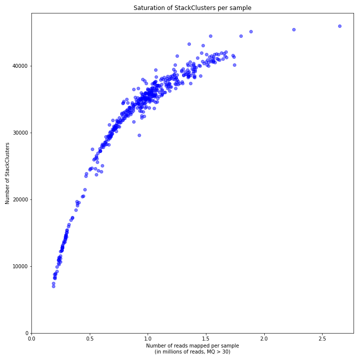
18 644 loci with completeness >80%
SNP calling and filtering
The Unified Genotyper tool of GATK was used to perform the SNP calling by comparing the mapped reads to the reference genome of C. canephora. We used the .bed file provided by SMAP delineate to only call SNPs within the 18644 loci with completeness higher than 80% across all 256 samples.
cd /path/to/bamfiles_folder
#Make a string variable that contains all input .bam files
BAM_FILES=( "*".BWA.bam )
for i in "${BAM_FILES[@]}"
do #make a variable STRING that contains all bam files, including the "-I" option that needs to precede the sample name in the GATK command
STRING+='-I '
STRING+="$i "
done
#Run docker
docker run -w /path/to/bamfiles_folder/ \
-v /path/in/host/to/link/:/path/in/container/to/link/ broadinstitute/gatk3:3.7-0 java \
-jar /usr/GenomeAnalysisTK.jar \
-R /path/to/reference_genome_fasta_file.fasta \
-T UnifiedGenotyper \
$STRING \
-o /path/to/output_directory/output_name.vcf \
-L /path/to/path_to_bed_file
Output: 239.007 SNPs
SNP and sample quality filter
This command filtered on:
Minimum average depth per sample of 30
Minimum allele count of 4
Minimum SNP quality of 20
Minimum genotype quality of 30
Minimum depth per sample of 10
vcftools --vcf /path/to/output_SNPcalling.vcf --min-meanDP 30 --mac 4 --minQ 20 --minGQ 30.0 --minDP 10.0 --recode --out output_SNP_and_sample_quality_filtered.vcf
Polymorphic SNP filtering
The SelectVariants tool of GATK was used to retain polymorphic SNPs.
docker run -v /path/in/host/to/link/:/path/in/container/to/link/ broadinstitute/gatk3:3.7-0 java \
-jar /usr/GenomeAnalysisTK.jar \
-T SelectVariants \
-R /path/to/reference_genome_fasta_file.fasta \
-V /path/to/SNP_and_sample_quality_filtered.vcf \
--excludeNonVariants \
-o output_polymorphic_SNPs_filtered.vcf
Biallelic SNP filtering
The SelectVariants tool of GATK was used to only retain biallelic SNPs.
docker run -v /path/in/host/to/link/:/path/in/container/to/link/ broadinstitute/gatk3:3.7-0 java \
-jar /usr/GenomeAnalysisTK.jar \
-T SelectVariants \
-R /path/to/reference_genome_fasta_file.fasta \
-V /path/to/output_polymorphic_SNPs_filtered.vcf \
-restrictAllelesTo BIALLELIC \
-o output_biallelic_SNPs_filtered.vcf
Output filtered SNPs: 3212 SNPs
Warning: GATK will use the file name of the bam file which is defined within the bam file as sample name. By changing the name of the bam file name manually or via the command line,
the sample will not be adapted in the .vcf file. Therefore, if you want to work with shorter or more informative names in further analyses,
we recommend to change the samples after SNP calling in the obtained .vcf file using this customized python script and an excel file containing the original .bam file names in one collumn and the preferred names in another column.
Checking for genetically identical individuals
Before analyzing the population structure, we want to make sure that every individual is a genetically unique individual. Normally DNA of every individual was extracted and sequenced once, but possible labeling errors during plant maintenance, sampling, DNA extraction,library preparation, or sequencing, may lead to identical fingerprints across the sample set, or the identification of clonal materials in the collection. Therefore, we check if each indiviudal in the sample set is unique by calculating the pairwise Jaccard Inversed Distance (JID) between all pairs of individuals using SMAP relatedness pairwise.
Haplotype calling
SMAP relatedness pairwise uses haplotype calls of each individual to calculate the pairwise Jaccard Inversed Distance (JID). Therefore, read-backed haplotyping was conducted based on the combined variation in SMAPs (obtained by SMAP delineate) and SNPs (obtained by GATK) using the SMAP haplotype-sites: module.
smap haplotype-sites /path/to/BAM /path/to/bed /path/to/vcf \
-mapping_orientation ignore \
--partial include \
--processes 16 \
--plot_type png \
--no_indels \
--min_distinct_haplotypes 2 \
--min_read_count 10 \
--min_haplotype_frequency 2 \
--discrete_calls dosage \
--frequency_interval_bounds 10 10 90 90 \
--dosage_filter 2
Output: 22602 haplotypes within 18644 loci
Genetic similarity
SMAP relatedness pairwise code:
smap relatedness pairwise --table /path/to/haplotype_table \
--input_directory /path/to/directory/of/haplotype/table \
--output_directory /path/to/output/directory/ \
--samples /path/to/sample_ID_file \
--processes 16 \
--plot_type png \
--locus_completeness 0.1
--similarity_coefficient Jaccard \
--locus_information_criterion Shared \
--partial
--print_sample_information All \
--print_locus_information All \
--plot_format png \
Alternative: you can also calculate the JID for a subset of individuals. To do so, you only list the individuals of the subset in the Sample_ID.txt file specified by the parameter –samples. The order of the samples within the JID matrix will be specified by the order of the individuals listed in the Sample_ID.txt file. You can also give your individuals an alternative name in the JID matrix by adding a second column to the sample ID text file indicating the new names.
First, we look at the distribution of the pairwise JID values to set a threshold to identify all pairs of genetically identical samples.
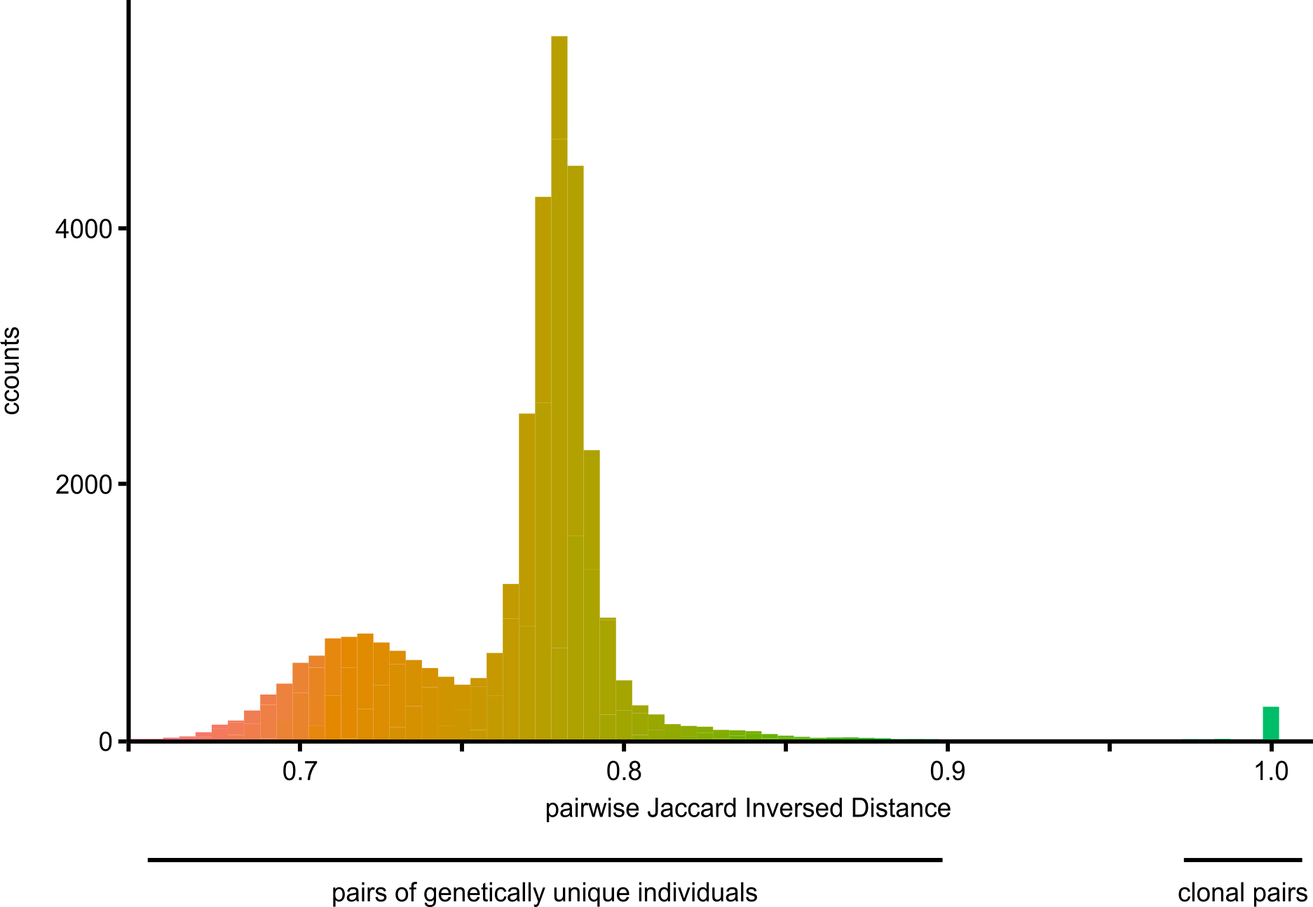
Distribution of JID values across all pairwise comparisons revealed a group of samples with pairwise JID in the range 0.974–1, and a separate group of sample pairs with pairwise Jaccard Inversed Distance ranging between 0.64 and 0.89. A JID of 1 means identical haplotype calls at all detected loci (i.e., genetically identical). In practice, a Jaccard Inversed Distance in the range of 0.974 to 1, means that one HiPlex locus out of all XX detected loci in the sample pair may display a different haplotype constitution between two samples. (for instance a single instance of a false negative or false positive detection of a haplotype, due to technical errors). Therefore, the minimal JID of 0.974 (for GBS data) was used as a threshold to identify all pairs of genetically identical samples (i.e., clones).
Second, genetically identical samples were identified using the minimal JID values of 0.974.
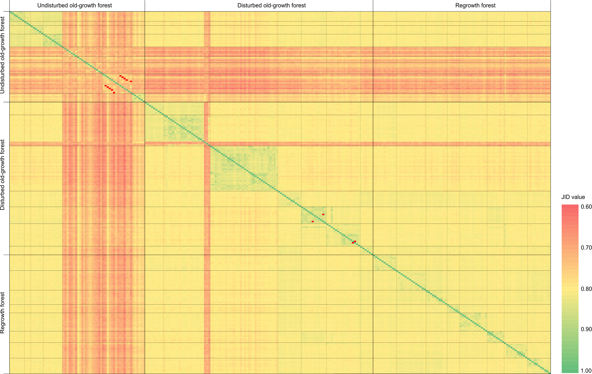
Seven pairs of samples (indicated in red) had a JID higher than 0.974 and were therefore identified as genetically identical samples. As Coffea canephora is a self-incompatible species we did not expect genetically identical samples in our sample set. By looking further at the genetically identical sample pairs, we discovered some repeats that indicated errors had been made during the creation of the GBS libraries in the lab. To prevent bias from these identical pairs in the population structure analyses, one individual of each identical sample pair (7 in total) was removed from the sample set.
Investigating the genetic structure and composition
Principal component analysis
A principal component analyses performed on the filtered 3212 SNPs for the remaining 249 wild C. canephora samples, will give us a first impression of the population structure within the wild coffee population. An annotation file is needed to annotate the samples with more information, such as sample ID, sampling location, location information, etc. The order of the samples in the annotation file needs to be the same as in the .vcf file
```
R script for PCA with SNP data
```
# *Install and load required packages*
library(vcfR)
library(adegenet)
library(ape)
library(tidyverse)
# *Set working directory*
setwd("/path/to/working_directory/")
getwd()
# *Read vcf file*
vcf <- read.vcfR("path/to/.vcf")
##Check vcf file
head(vcf)
vcf@fix[1:10,1:5]
## Convert vcf to Genlight object*
gen <- vcfR2genlight(vcf)
## Add real SNP names
locNames(gen) <- paste(vcf@fix[,1],vcf@fix[,2],sep="_")
# *Perform a PCA*
pca <- glPca(gen, nf=100) #principal component analysis with 100 PCs
plot(pca$scores)
pca_scores <- as.data.frame(pca$scores)
## Check the proportion of variance explained by the first three PC axes
pca$eig[1]/sum(pca$eig)
pca$eig[2]/sum(pca$eig)
pca$eig[3]/sum(pca$eig)
# Create a dataframe with the annotation file and PCA scores
## Import annotation file
annotations <- read.delim("Annotations.txt", sep = "\t", header = TRUE)
### WARNING: The order and names of the individuals must be the same as in the VCF file.
## Create a new dataframe containing a first column wiht Sample_IDs and other columns containing the PCA scores
pca_annotated <- cbind(annotations, pca$scores[,c(1:3)])
# Plot the PCA
pca_plot <- ggplot(pca_annotated,aes(x = PC1,y = PC2, color = Plot_nr, shape = Forest_disturbance))+
geom_point(size=2.5)+
#scale_color_manual(values = c("blue", "red", "green"))+
ggtitle("Wild C. canephora population")+
xlab("PC1 (5.1%)")+
ylab("PC2 (3.2%)")+
theme_bw()
pca_plot
write.table(pca_annotated, "pca_scores.txt", sep="\t", row.names = FALSE)
png("output_file_name.png", width = 900, height = 600)
pca_plot
dev.off()
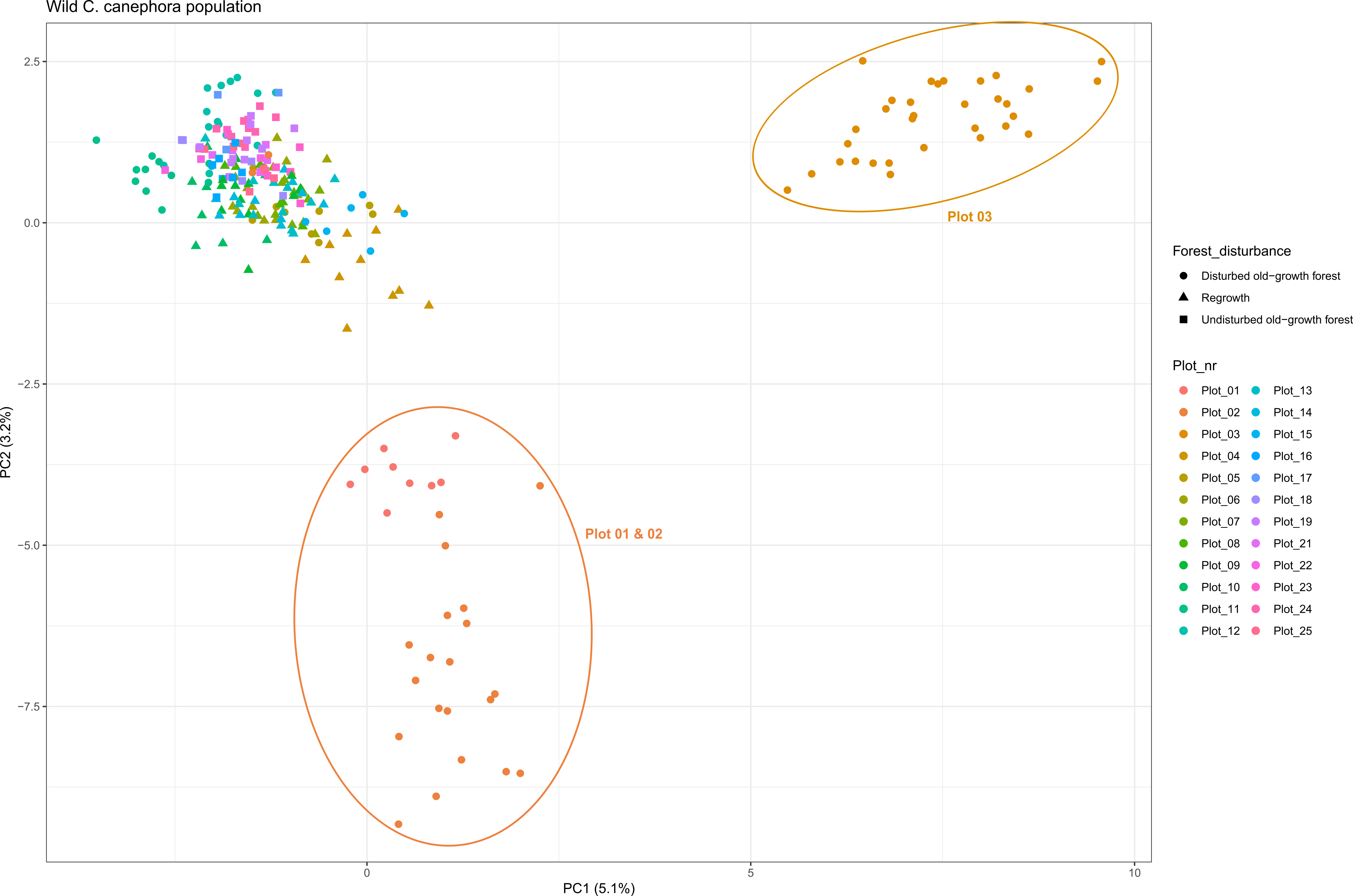
Three different clusters could be identified using the PCA analyses. All samples collected in plot 3 clustered together on the positive PC1-axis and all samples collected in plot 1 and 2 clustered together on the negative PC2-axis. All other samples (plot 4-25) clustered together on the negative PC1-PC2-axis.
As the samples are clustered together based on their geographical location, rather than forest disturbance, we have an indication that the geographical location could be a main driver of genetic structure in this wild coffee population. To support this hypothesize, we will analyze the genetic structure using the fastSTRUCTURE analysis.
fastSTRUCTURE
To visualize the genetic structure and genetic composition of the wild coffee population, fastSTRUCTURE was run using a PLINK formatted genotype call file.
vcftools --vcf /path/to/SNP_filtered_vcf_file.vcf --plink --out output_file_name
Converting .vcf file to .plink format creates a .map and .ped file.
The .map file contains information about the SNP: Chromosome name, SNP name, Position in Morgans or centiMorgans (optional) and basepair coordinates. However, when our .vcf file was converted to the .map file, the column with the Chromosome names consisted of zeros instead of the chromosome numbers. Without adjusting the first column the fastSTRUCTURE analyses will give an error. Therefore, the chromosome numbers were manually added to the .map file based on the SNP name.
The .ped file contains information about the sample set: Family ID, Individual ID, Father ID, Mother ID, Sex, Phenotype, Rest of the columns: Genotypes for each SNP. However, when our .vcf file was converted to the .ped file, the column which should contain the family ID contained also the individual ID. This is because the .vcf file does not contain any population or sample information besides the sample ID. Therefore, the plot information was manually added to the .ped file based on the annotation file used for the principal component analyses. WARNING: make sure there are no spaces in the family name otherwise plink will read this as too many tokens.
Next, the .ped and .map file are converted to a .bed file .. code:: ruby
plink –file /path/to/vcf_to_plink_output –make-bed –out output_file_name
Using this .bed file, we can run the fastSTRUCTURE analysis. As we currently not know how many clusters are present in our sample set we will loop the analyses for 2 to 9 clusters.
conda activate faststructure
for i in `seq 2 9`; do structure.py --input=/path/to/plink_bed_file(no_suffix) --output=output_file_name -K $i --full --seed=100; done
- For each cluster, 5 output files are created:
meanQ: mean ancestry proportion per sample
example meanQ (K=4)meanP: mean error rate of proportion per sample
example meanP (K=4)varQ: variance of mean ancestry proportion per sample
example varQ (K=4)varP: variance of mean error rate of proportion per sample
example varP (K=4)
- Note: Each line in the output file corresponds with a sample but the sample name is not given in the output. The order of the samples in the output files is the same as the order in the vcf and plink files.
Each column in the output file corresponds to a cluster.
The chooseK.py script was used to get the optimal number of clusters, which is printed to the terminal. .. code:: ruby
conda activate faststructure
chooseK.py –input path/to/output_name_fastSTRUCTURE(no_suffix)
output: Model complexity that maximizes marginal likelihood = 4
The optimal number of clusters found in the wild coffee population was 4. A new file was manually made were the meanQ results belonging to the K = 4 were complemented with a sample ID, plot number and forest disturbance info so that the fastSTRUCTURE result can be visualized in RStudio.
visualizing fastSTRUCTURE using R-script``` R script to visualize fastSTRUCTURE results ``` #Install and load required packages library(adegenet) library(tidyverse) #Set working directory setwd("/path/to/working/directory") getwd() #Read manually made faststructure file fs <- read_delim("R_plot_faststructure.txt", delim = "\t", col_names = TRUE) #Making the barplot ggplot(fs, aes(fill=Cluster, y=Value, x=Number)) + geom_bar(position="stack", stat="identity", width = 1) + theme(axis.text.x=element_blank(), axis.ticks.x=element_blank(), axis.text.y=element_blank(), axis.ticks.y=element_blank(), axis.title.x = element_blank(), axis.title.y = element_blank(), panel.grid.major = element_blank(), panel.grid.minor = element_blank(), panel.background = element_blank())+ facet_grid(~ Forest, scales = "free_x", space = "free_x", switch = "x")
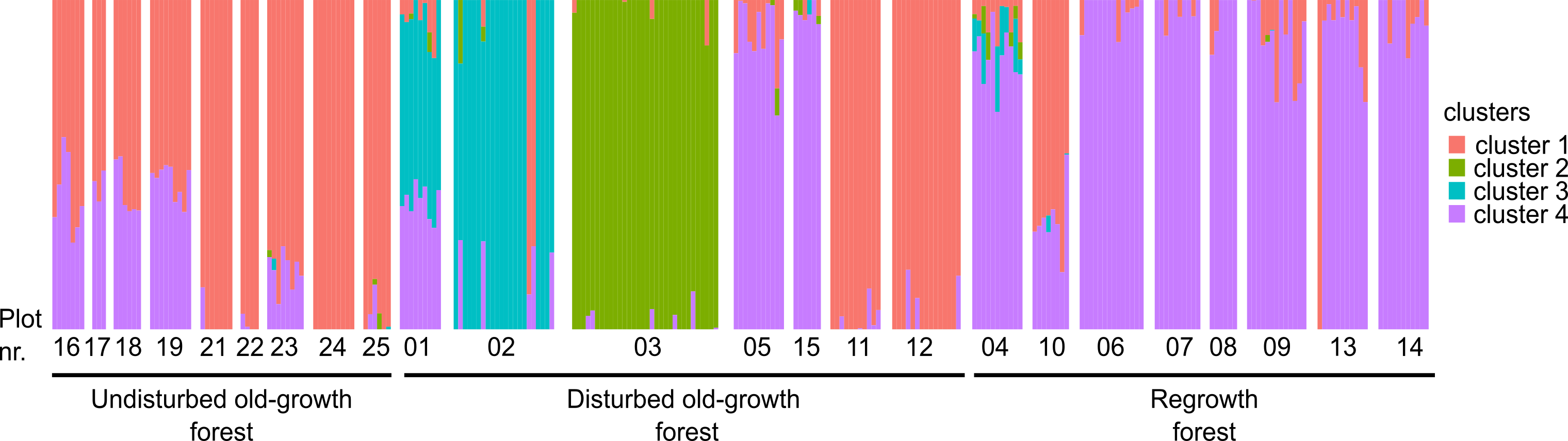
The fastSTRUCTURE analysis showed that the plots in undisturbed old-growth forest were divided into two subpopulations, namely plot 16–19 and plot 21–25, with individuals in plots 16–19 showing a mixture of DAPC cluster 1 and 4. Plots in disturbed old-growth forest were divided into four subpopulations, namely: plots 1 and 2; plot 3; plots 5 and 15; plots 11 and 12. Plots in regrowth forest were divided into three subpopulations, namely: plot 4; plot 10; plots 6–9, 13 and 14. Individuals in plot 10 showed to be a mixture of clusters 1 and 4, whereas individuals in plot 4 showed a mixture of all DAPC clusters. Overall, clustering of the samples from old-growth forest was differentiated according to the geographical location of the plots.
Isolation-by-distance
The PCA and fastSTRUCTURE showed genetic structure within the wild coffee population mainly driven by geographical location. To see if this could be a result of isolation-by-distance (IBD), we will calculate genetic distances between the plots, pairwise Fst values (Weir and Cockerham, 1984), using PLINK 1.9 and correlated these genetic distances to the geographical distances between the plots. Therefore, we will use the plink files (also used for fastSTRUCTURE analysis), a list of all plots and a python script:
popfile = "list_lots.txt" #List of populations - one per line
plinkfile = "wild_coffee" #Just the bit before the .bim etc.
import os
#Add pop names to a list
dd = open(popfile)
pops = []
for line in dd:
pops.append(line.strip())
dd.close()
output = open("pairwise_fst.txt","w")
#Now do a pairwise loop over populations
for i in range(0,len(pops)-1):
for j in range(i+1,(len(pops))):
temp = open("temp.txt","w")
temp.write(pops[i] + ("\n") + pops[j])
temp.close()
os.system("plink --bfile " + plinkfile + " --fst --family --keep-fam temp.txt --out temp --autosome-num 37")
cd = open("temp.log")
for line in cd:
if line.startswith("Mean Fst"):
output.write(pops[i] + ("\t") + pops[j] + ("\t") + line.split()[3] + ("\n"))
break
os.system("rm temp.*")
output.close
Output: a text file with the pairwise Fst value (column 3) between the first plot (column 1) and second plot (column 2) To visualize the comparison between plots from different forest disturbance levels (undisturbed, disturbed, and regrowth) an extra column will be manually added to the text file indicating the level of disturbance per plot.
..code-block:: r
` R script to visualize IBD `#Install and load required packages library(tidyverse) library(ggplot2) library(ggthemes) library(geosphere)
#Set working directory
setwd(“/path/to/working/directory”)
#Read pairwise Fst file
pfst <- read_delim(“pairwise_fst.txt”, delim = “t”,col_names = T) # read in pairwise Fst file pfst
colnames(pfst) <- c(“group”, “p1”,”p2”,”FST”) # give the columns a name pfst
ll <- read_delim(“latlong_no20.txt”, delim = “t”) ll
#Calculate pairwise distance between each of our populations
##Create an empty distance column pfst$dist <- NA pfst
- ##Loop over the pfst data frame
for(i in 1:nrow(pfst)) {
###Extract population names from pd data frame pop1 <- pfst$p1[i] #First element of p1 column pop2 <- pfst$p2[i] #First element of p2 column
###Get lat and long information l1 <- subset(ll,Population == pop1) l2 <- subset(ll,Population == pop2)
###Now calculate distance pfst$dist[i] <- distGeo(p1 = cbind(l1$Long,l1$Lat), p2 = cbind(l2$Long,l2$Lat))
}
##Check that it worked head(pfst)
## Save table
write.csv(pd, file=”pd.csv”)
#Plot pairwise Fst vs geographical distance between pairs of plots
ggplot(pfst,aes(x = dist/1000,y = FST, color = pfst$group))+ #divide by 1000 to get distance in km geom_point(aes(size = 0.5))+ scale_color_manual(values = c(“#990000”,”#FFCC99”,”#FF6600”,”#333999”, “#99CCFF”, “#CCCCFF”))+ theme_bw()+ xlab(“Distance (km)”)+ ylab(expression(“F”[ST]))+ geom_abline()+ geom_smooth(method = lm, se =FALSE, colour = “black”)+ xlim(NA,45)+ ylim(0,0.14)+ guides(color=guide_legend(title=”Forest disturbance”), size=”none”)
Isolation-by-distance was found across all plots explaining the genetic structure found in the wild coffee population.
Establishing a core collection
The wild coffee population in the Yangambi region harbours a high degree of genetic diversity and therefore is a very important genetic resource. To ensure that this high genetic diversity will be preserved, we could opt to create a core collection of this wild population. Genetic data, phenotypical data or agricultural traits can all be taken into account to select the best samples for the core collection, but for this wild coffee population, only the genetic data is currently available.
Core Hunter 3 v3.2.0 R package (De Beukelaer et al., 2018) was used to test two core collection strategies for the 248 samples of the wild coffee population:
Maximization strategy (CC-I): maximizes the genetic diversity by selecting the most diverse loci
Genetic distance method (CC-X): maximizes the genetic distance between the entries of the core collection and selecting the most diverse plant material within the wild coffee population
For both core collection strategies, allele coverage (CV), diversity within and between alleles [He and Shannon’s index (SH)], and average genetic Modified Roger’s (MR) distance between entry-accession (AN) and entry-to-nearest-entry (EN) were calculated for nine different core sizes (3, 5, 10, 25, 50, 100, 150, 200, and 249 accessions).
The filtered .vcf file will be manually converted to the format needed for CoreHunter. The genotype calls (0/0, 0/1 and 1/1) will be transformed into diploid dosage (0,1,2) and the SNPs rows will be transposed with the sample columns whereby the columns contain data per SNP and the rows contain data per sample. Additionally, if a sample had no genotype call for a specific SNP (./.) this cell will be left empty.
..code-block:: r
` R script to visualize IBD `# Install and load required packages library(rJava) library(corehunter) library(ggplot2) library(patchwork) library(cowplot) library(tidyverse)# Import genotype data file genoo <- genotypes(file = “Input_CoreHunter.txt”, format = “biparental”)
# Create CoreHunter data file my.data <- coreHunterData(genoo) my.data
# Test Maximization strategy (CC-I)
## Create empty dataframe to add diversity and distance measures score_CCI <- data.frame(“Size” = numeric(0), “Average entry-to-nearest-entry distance” = numeric(0), “Average accession-to-nearest-entry distance” = numeric(0), “Shannon’s Index” = numeric(0), “Expected heterozygosity”=numeric(0), “Allele coverage”= numeric(0))
for (i in seq(2,(length(genoo$ids)-1),10)) {
## Create core collection with desired size core <- sampleCore(my.data, objective(“AN”, “MR”), size = i, steps = 500)
## Calculate diversity and distance measures within the core collection EN_MR <- evaluateCore(core, my.data, objective(“EN”, “MR”)) AN_MR <- evaluateCore(core, my.data, objective(“AN”, “MR”)) CV <- evaluateCore(core, my.data, objective(“CV”)) SH <- evaluateCore(core, my.data, objective(“SH”)) HE<- evaluateCore(core, my.data, objective(“HE”))
score_CCI[nrow(score_CCI)+1,] <- data.frame(‘Size’ = i, “Average entry-to-nearest-entry distance” = EN_MR, “Average accession-to-nearest-entry distance” = AN_MR, “Expected heterozygosity” = HE, “Shannon’s Index” = SH, “Allele coverage” = CV) }
# Test distance method (CC-X)
## Create empty dataframe to add diversity and distance measures score_CCX <- data.frame(“Size” = numeric(0), “Average entry-to-nearest-entry distance” = numeric(0), “Average accession-to-nearest-entry distance” = numeric(0), “Shannon’s Index” = numeric(0), “Expected heterozygosity”=numeric(0), “Allele coverage”= numeric(0))
for (i in seq(2,(length(genoo$ids)-1),10)) {
## Create core collection with desired size core <- sampleCore(my.data, objective(“EN”, “MR”), size = i, steps = 500)
## Calculate diversity and distance measures within the core collection EN_MR <- evaluateCore(core, my.data, objective(“EN”, “MR”)) AN_MR <- evaluateCore(core, my.data, objective(“AN”, “MR”)) CV <- evaluateCore(core, my.data, objective(“CV”)) SH <- evaluateCore(core, my.data, objective(“SH”)) HE <- evaluateCore(core, my.data, objective(“HE”))
score_CCX[nrow(score_CCX)+1,] <- data.frame(‘Size’ = i, “Average entry-to-nearest-entry distance” = EN_MR, “Average accession-to-nearest-entry distance” = AN_MR, “Expected heterozygosity” = HE, “Shannon’s Index” = SH, “Allele coverage” = CV)}
# Evaluation of the diversity and distance measures
color_list <- c(“#339999”, “#006699”, “#FF9966”, “#CC6666”, “#66CC66” ) measure_list <- c(“Average entry-to-nearest-entry distance”, “Average accession-to-nearest-entry distance”, “Expected heterozygosity”, “Shannon’s Index”, “Allele coverage”) plots <- list() count <- 1
## Create plots for all calculated diversity and distance measures ### WARNING: this codes needs to be run twice: once for CC-I and once for CC-X for (measure in colnames(score_CCX[2:6])) { subtitle <- measure_list[count] plot <- ggplot(score_CCX, aes(x=Size, y= .data[[measure]]))+ geom_point(colour = color_list[count])+ geom_line(colour = color_list[count])+ scale_x_continuous(breaks = seq(min(score_CCX$Size), max(score_CCX$Size), by = 20))+ ggtitle(measure_list[count])+ theme_bw()+ theme(legend.position = “none”, plot.title = element_text(color = color_list[count], size = 12, hjust = 0.5), axis.title.y = element_blank())
plots[[measure]] <- plot count <- count + 1 }
combined_plot <- wrap_plots(plots, ncol=2)+ plot_annotation(title = “Core collection CC-X”, theme = theme(plot.title = element_text(hjust=0.5))) combined_plot
# Create core collection with optimized core size
## Core collection CC-I
CCI <- sampleCore(my.data, objective(“AN”, “MR”), size = 122) CCI_samples <- data.frame(‘Sample_ID’ = CCI$sel) ##save sample ids of the selected samples
## Core collection CC-X CCX <- sampleCore(my.data, objective(“EN”, “MR”), size = 22) CCX_samples <- data.frame(‘Sample_ID’ = CCX$sel) ##save sample ids of the selected samples
# Visualization of core collection samples using PCA
## Here we will use the pca values, which were already calculated in a previous analysis
## Import pca scores
pca <- read_delim(“pca_scores.txt”, delim = “t”, col_names = TRUE)
## Create a column in a new dataframe with the information if the individual is selected as ## an entry for core collection CCI, CCX or both
cc_info <- data.frame(‘Sample_ID’ = as.character(pca$Sample_ID))
cc_info <- Collection %>% mutate(Collection = case_when( cc_info$Sample_ID %in% CCI_samples$Sample_ID & !(cc_info$Sample_ID %in% CCX_samples$Sample_ID) ~”CC-I”, cc_info$Sample_ID %in% CCX_samples$Sample_ID & !(cc_info$Sample_ID %in% CCI_samples$Sample_ID) ~”CC-X”, cc_info$Sample_ID %in% CCI_samples$Sample_ID & cc_info$Sample_ID %in% CCX_samples$Sample_ID ~”CC-I and CC-X”, TRUE ~ “Not in core collections” ))
## Merge the new dataframe with the pca values pca_info <- merge(cc_info, pca, by = “Sample_ID”)
## Create plot
pca_plot <- ggplot(pca_info, aes(PC1, PC2, color = Collection))+ geom_point(alpha = 0.4, size = 3)+ xlab(“PC1 ()”)+ ylab(“PC2 ()”)+ ggtitle(“PCA core collections of wild coffee population”)+ guides()+ theme_bw()
pca_plot
CC-I For CC-I, an optimal core size was determined based on maximized genetic diversity (He and SH) and minimized AN distance.
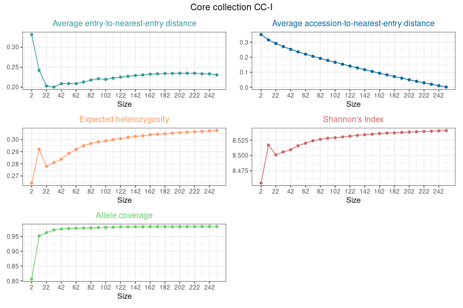
The optimal core size comprised 100 unique genetic fingerprints as the genetic diversity was higher than other core sizes (He of 0.20 and SH of 5.75), all alleles were accounted for (CV of 1) and entry-to-accession distance was low (AN of 0.13)
CC-X For CC-X, an optimal core size was determined based on maximized genetic diversity (He and SH) and maximized EN distance.
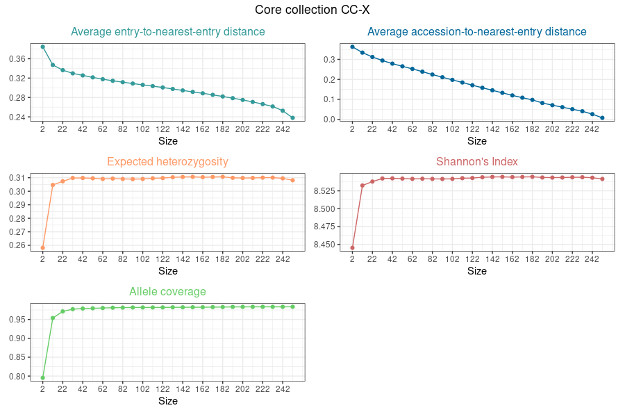
The optimal core size comprised 10 unique genetic fingerprints as the genetic diversity (He of 0.23 and SH of 5.79) was higher than other core sizes tested for CC-X, almost all alleles were accounted for (CV of 0.93) and entry-to-nearest-entry distance was high (EN = 0.35).
Using the values of the PCA, which we had created earlier, we can show which of the samples were selected for the core collections CC-I and CC-X
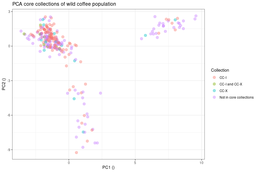
On the plot we can see that accessions assigned to the CC-I and CC-X core collection were evenly distributed across the ordination space of the wild coffee population.
Characterization of the genetic composition and establishment of a core collection of cultivated C. canephora using HiPlex SNP markers
Purpose
The genetic background of a Coffea canephora cultivar collection grown in the Congo Basin was analysed to determine the different genetic sources of the crop. HiPlex sequencing using 86 loci was performed on 270 C. canephora samples and 9 samples were genotyped using GBS. In addition, HiPlex sequencing with the same loci was performed on 48 samples of local wild C. canephora and 35 samples of a variety of coffee species. At last, whole genome shotgun (WGS) sequencing data of two reference samples of the Congolese subgroup A was retrieved from SRA (Bioproject PRJNA803612). After sequencing, the following workflow was executed to visualize the population structure of coffee in the Congo Basin:
Reads were mapped to the reference genome of C. canephora using Burrow-Wheeler Aligner Maximal Exact Match (BWA-MEM)
Calling SNPs with GATK and BCFtools
Determining haplotypes by executing SMAP haplotype-sites
Analysis of the population structure in four different ways:
First indication of the genetic structure using principal component analysis (PCA)
Genetic clusters of the samples set with fastSTRUCTURE
Genetic distances between samples using SMAP genetic relationship matrices (SMAP relatedness pairwise)
Creation of a Phylogenetic tree
Creating a Core collection
Installation of software
Downloading the specific software versions used in this tutorial will ensure all displayed commands operate properly. The latest software versions can also be downloaded.
-
Using wget and virtual environment:
wget https://gitlab.com/truttink/smap/-/archive/4.6.5/smap-4.6.5.tar.bz2 tar -xvf smap-4.6.5.tar.bz2 cd smap-4.6.5/ python3 -m venv .venv source .venv/bin/activate pip install --upgrade pip pip install . #Test if installation was successful: smap delineate --version #Output: (date) root - INFO: This is SMAP 4.6.5 (date) Delineate - INFO: SMAP-delineate started. 4.6.5
-
wget https://bitbucket.org/kokonech/qualimap/downloads/qualimap_v2.2.1.zip unzip qualimap_v2.2.1.zip cd qualimap_v2.2.1 #Test if installation was successful: ./qualimap multi-bamqc #Output (first part): Java memory size is set to 1200M Launching application... QualiMap v.2.2.1 Built on 2016-10-03 18:14 Selected tool: multi-bamqc #Possible error when using newer Java versions: Java memory size is set to 1200M Launching application... Unrecognized VM option 'MaxPermSize=1024m' Error: Could not create the Java Virtual Machine. Error: A fatal exception has occurred. Program will exit. #Fix by editing qualimap file: nano ./qualimap #Change -XX:MaxPermSize=1024m to new java option: -XX:MaxMetaspaceSize=1024m #Test installation again
-
Install locally:
wget https://github.com/samtools/bcftools/releases/download/1.13/bcftools-1.13.tar.bz2 tar -xvf bcftools-1.13.tar.bz2 cd bcftools-1.13/ ./configure #if error => install dependencies depending on your OS (packages stated in terminal) #=> ./configure make sudo make install #Test if installation was successful: bcftools --version #Output: bcftools 1.13 Using htslib 1.13 Copyright (C) 2021 Genome Research Ltd. License Expat: The MIT/Expat license This is free software: you are free to change and redistribute it. There is NO WARRANTY, to the extent permitted by law.
Or install BCFtools docker image:
docker pull staphb/bcftools:1.13 #Test if installation was successful: docker run staphb/bcftools:1.13 bcftools --version #Output: bcftools 1.13 Using htslib 1.13 Copyright (C) 2021 Genome Research Ltd. License Expat: The MIT/Expat license This is free software: you are free to change and redistribute it. There is NO WARRANTY, to the extent permitted by law.
-
docker pull broadinstitute/gatk3:3.7-0 #Test if installation was successful: docker run broadinstitute/gatk3:3.7-0 java -jar /usr/GenomeAnalysisTK.jar --version #Output: 3.7-0-gcfedb67
-
Install locally:
wget https://github.com/vcftools/vcftools/releases/download/v0.1.16/vcftools-0.1.16.tar.gz tar -xvzf vcftools-0.1.16.tar.gz cd vcftools-0.1.16/ ./configure #if error => install dependencies depending on your OS (packages stated in terminal) #=> ./configure make sudo make install #Test if installation was successful: vcftools --version #Output: VCFtools (0.1.16)
Or install VCFtools docker image:
docker pull biocontainers/vcftools:v0.1.16-1-deb_cv1 #Test if installation was successful: docker run biocontainers/vcftools:v0.1.16-1-deb_cv1 vcftools --version #Output: VCFtools (0.1.16)
-
Install locally:
mkdir PLINK1.19 cd PLINK1.19 wget http://s3.amazonaws.com/plink1-assets/plink_linux_x86_64_20200616.zip unzip plink_linux_x86_64_20200616.zip #Move to a directory in PATH environment variable #for command line tool execution (e.g. /usr/bin) sudo mv plink /usr/bin/ #Test if installation was successful: plink --version #Output PLINK v1.90b6.18 64-bit (16 Jun 2020)
Or install PLINK docker image:
docker pull elixircloud/plink:1.9-cwl #Test if installation was successful: docker run elixircloud/plink:1.9-cwl plink --version #Output: PLINK v1.90p 64-bit (16 Jun 2020)
-
First install conda
Add Bioconda channel
Then install the fastSTRUCTURE conda environment:
conda create --name faststructure python=2.7 conda activate faststructure conda install -c bioconda faststructure #Test if installation was successful: chooseK.py #Output: Here is how you can use this script Usage: python /home/guest/miniconda3/envs/fastStructure/bin/chooseK.py --input=<file>
-
renv package is used for version control
-
docker pull broadinstitute/gatk:latest
Read mapping quality control
The method for read mapping quality control (QC) depends on the NGS method. Mapping quality can be evaluated with QualiMap for WGS, GBS and HiPlex reads. SMAP provides a more specific means of QC for mapped GBS reads: SMAP delineate.
SMAP delineate gives us insight into locus completeness and sequencing read depth across all samples. This is important for our workflow because no variants can be identified in samples where no reads are mapped in polymorphic regions.
smap delineate *path_to_GBS_bam_files* -mapping_orientation ignore -p 8 --plot all --plot_type png -f 50 -g 300 --min_stack_depth 2 --max_stack_depth 500 --min_cluster_depth 10 --max_cluster_depth 1500 --max_stack_number 2 --min_stack_depth_fraction 10 --completeness 1 --max_smap_number 10
Parameters were set for double-enzyme GBS with merged reads in diploid individuals as described in SMAP delineate examples.
The quality of the mapped reads is depicted by the MergedCluster barplots and the saturation curve scatterplot.
Median read depth per Mergedcluster
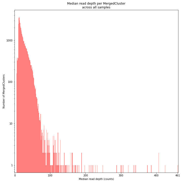
The median read depth per MergedCluster barplot depicts how many MergedClusters are shared between at least half of the samples at a given depth. The completeness of the mapped reads can be determined by comparing the individual StackCluster read depth barplots to this one.
All of our GBS samples have very similar read mapping distributions.
Mergedcluster completeness across samples
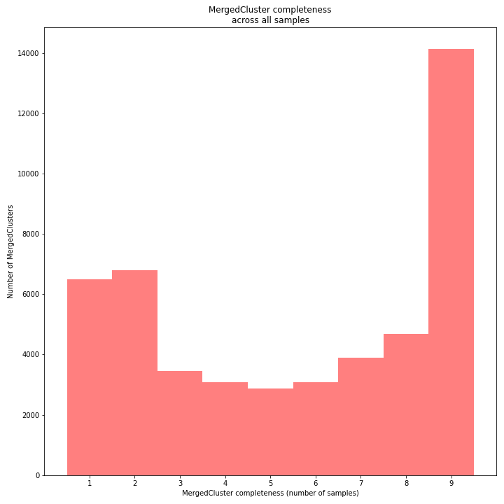
This barplot shows the distribution of MergedClusters completeness across all samples. A MergedCluster is plotted at x-value 1 if that MergedCluster only has a sufficient read depth in one sample. In contrast, MergedClusters with sufficient read depth across all samples are plotted at the maximal x-value (number of samples in the sample set).
Around 14000 MergedClusters are shared across all our samples because they have sufficient read depth in all samples (x = 9). Still, a lot of diversity if present judging by the high number of MergedClusters with no sufficient read depth for some samples.
SMAPs per MergedCluster
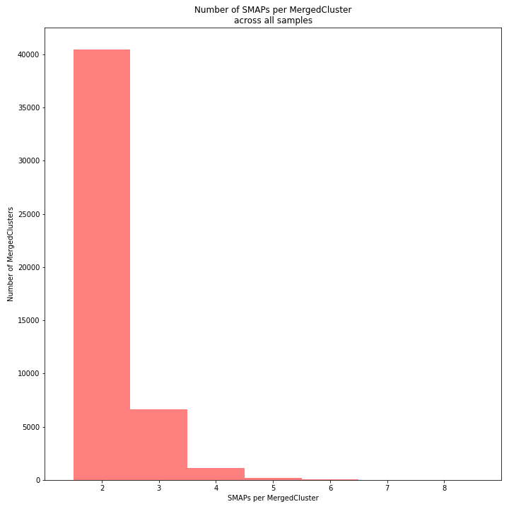
The abundance of read mapping polymorphisms is depicted in the SMAPs per MergedCluster barplot. All MergedClusters where reads have the same read mapping start and end positions contain 2 SMAPs. InDels and SNPs cause an increased number of SMAPs per MergedCluster.
Around 7000 MergedClusters display read mapping polymorphisms in the samples with GBS data.
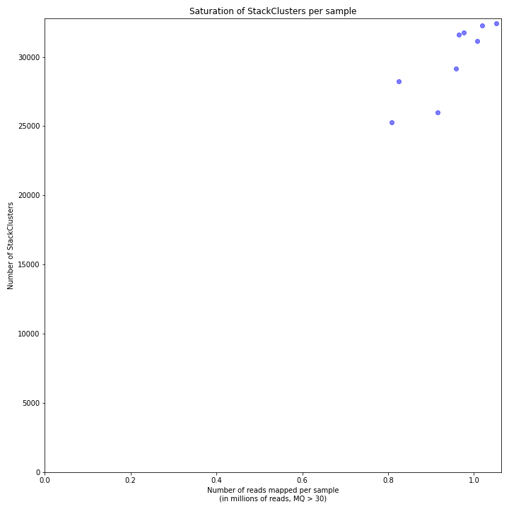
The detection of MergedClusters in function of the number of mapped reads is depicted in the saturation scatterplot. Samples are sequenced at a sufficient depth when increasing the depth yields no substantial increase in detected MergedClusters (= saturation point).
It is difficult to say whether the samples with the highest number of mapped reads have reached the saturation point. More GBS samples should be included in the experiment to determine this. However, the three samples with the lowest number of mapped reads are most likely not sequenced at a sufficient depth.
Qualimap Multi-sample BAM QC can be executed on all kinds of sequencing data. In addition, a bed or gff file with regions of interest can be provided to the tool which greatly reduces the execution time. A text file containing one column with sample names and a second column with the path to the respective bam file has to be provided.
cd qualimap_v2.2.1/
./qualimap multi-bamqc -d *file_with_file_names/paths* -r -gff *bed/gff_file_with_regions* -outdir *path_to_output*
Multi-sample BAM QC outputs summary statistics, evaluation graphs, as well as sample specific evaluations. We will only focus on summary statistics in the tabs below.
Globals
| Number of samples | 353 |
| Total number of mapped reads | 104,638,300 |
| Mean samples coverage | 2,618.76 |
| Mean samples GC-content | 41.62 |
| Mean samples mapping quality | 59.6 |
The summary statistics give a quick overview of the overall mapping quality of the samples. Check the samples statistics for sample-by-sample mapping quality scores.
Mapping quality is a phred-scaled probability of the read alignment being correct. For example, scores of 30 and 60 imply a read has a probability of 99.9% and 99.9999%, respectively, of being mapped correctly.
Sample coverage refers to the average number of times each base in the reference genome sequence is covered by reads. A coverage of 30 is considered the lower limit for many applications.
HiPlex performs very well for sample coverage. This was expected because the sequencing method specifically targets these regions. The mapping quality is also very good.
Summary
Globals
| Number of samples | 9 |
| Total number of mapped reads | 8,784,773 |
| Mean samples coverage | 35.14 |
| Mean samples GC-content | 40.31 |
| Mean samples mapping quality | 59.66 |
GBS samples have a much lower coverage than HiPlex but still pass the threshold of 30. Mapping quality is similar to HiPlex.
Summary
Globals
| Number of samples | 2 |
| Total number of mapped reads | 487,563,633 |
| Mean samples coverage | 67.19 |
| Mean samples GC-content | 40.09 |
| Mean samples mapping quality | 59.58 |
The two WGS samples have double the coverage compared to GBS, but it is still a lot lower than HiPlex. The mapping quality is again more than adequate.
Calling SNPs
Next, BCFtools and GATK were compared for SNP calling. Polymorphisms were identified, SNPs were selected and filtered on position and quality.
SNP calling
The Unified Genotyper tool of GATK was used to perform the SNP calling by comparing the mapped reads to the reference genome of C. canephora. We provided a bed file containing the HiPlex loci regions because we are only interested in the SNPs inside them. This region-specific SNP calling greatly reduces computation time. The reference genome bed file has to be included if you need to call SNPs in the entire genome. A lot more resources are required for complete SNP calling but it can be worthwhile if the vcf file will be used in more pipelines.
docker run -w *working_directory_in_container* -v *path_in_host_to_link*:*path_in_container_to_link* broadinstitute/gatk3:3.7-0 java -jar /usr/GenomeAnalysisTK.jar \
-R *path_to_reference_genome_fasta_file* \
-T UnifiedGenotyper -I *file_with_bam_files* \
-o *path_to_vcf_file* \
-L *path_to_bed_file*
The command also needs a .list file that contains all bam file names (\n separated).
The following command was used to determine the number of SNPs:
grep -v ^# *path_to_vcf_file* | wc -l
output: 12130453
SNP filtering
Amplicon region filter
After complete calling it is still possible to filter for SNPs inside the specified amplicon regions with following command:
vcftools --vcf *path_to_vcf_file* --bed *path_to_bed_file* --recode --recode-INFO-all --out *path_to_output_1*
output:
After filtering, kept 364 out of 364 Individuals
Outputting VCF file...
After filtering, kept 1230 out of a possible 12130453 Sites
Run Time = 201.00 seconds
VCFtools was used to only retain SNPs inside the amplicon regions.
It is possible the following warning is printed in the terminal:
Example warning:
Warning: Expected at least 2 parts in FORMAT entry: ID=PL,Number=G,Type=Integer,Description="Normalized, Phred-scaled likelihoods for genotypes as defined in the VCF specification">
VCFtools does not expect commas in the description tag of the header lines. This warning did not have an influence on our input but if so, the warning can be prevented by removing/changing all commas in the description.
SNP/sample quality filter
vcftools --vcf *path_to_output_1* --min-meanDP 30 --mac 4 --minQ 20 --minGQ 30.0 --minDP 10.0 --recode --out *path_to_output_2*
Output:
After filtering, kept 364 out of 364 Individuals
Outputting VCF file...
After filtering, kept 415 out of a possible 1230 Sites
Run Time = 0.00 seconds
This command filtered on:
Minimum average depth per sample of 30
Minimum allele count of 4
Minimum SNP quality of 20
Minimum genotype quality of 30
Minimum depth per sample of 10
Polymorphic SNP filtering
docker run -v *path_in_host_to_link*:*path_in_container_to_link* broadinstitute/gatk3:3.7-0 java -jar /usr/GenomeAnalysisTK.jar \
-T SelectVariants \
-R *path_to_reference_genome_fasta_file* \
-V *path_to_output_2* \
--excludeNonVariants \
-o *path_to_output_3*
The SelectVariants tool of GATK was used to retain polymorphic SNPs. The command does not output information about the filtering in the terminal.
Check SNP number:
grep -v ^# *path_to_output_3* | wc -l
output: 415
Previous filtering apparently already removed non-polymorphic sites.
Biallelic SNP filtering
docker run -v *path_in_host_to_link*:*path_in_container_to_link* broadinstitute/gatk3:3.7-0 java -jar /usr/GenomeAnalysisTK.jar \
-T SelectVariants \
-R *path_to_reference_genome_fasta_file* \
-V *path_to_output_3* \
-restrictAllelesTo BIALLELIC \
-o *path_to_output_4*
Example terminal output (for subset of 10 samples).
Next, the SelectVariants tool of GATK was used to only retain biallelic SNPs.
Check SNP number:
grep -v ^# *path_to_output_4* | wc -l
output: 402
The result of the SNP calling and filtering with GATK/VCFtools was a total of 402 SNPs. This is be compared with BCFtools in the next tab.
SNP calling
The second used SNP calling tool was BCFtools.
bcftools mpileup -R *path_to_bed_file* -Ou -a FORMAT/AD,FORMAT/DP -f *path_to_reference_genome_fasta_file* --bam-list *path_to_list_bam_files* \
| bcftools call --skip-variants indels -mv -Ov -a GQ -o *path_to_vcf_file*
First, genotype likelihoods at each covered genomic position were created with bcftools mpileup. The number of high-quality bases (DP) and allelic depth (AD) that will later be used to filter was added to the format column. Optionally, the mpileup analysis can be reduced to regions present in a bed file with the -R option. mpileup needs a .txt file that contains all bam file names (\n separated).
Next, BCFtools call performs the actual SNP calling. The option -a GQ was provided to include the genotype quality for filtering and InDels were skipped with the option –skip-variants indels.
BCFtools does not give any terminal output regarding information about the execution time. This must be determined ourselves.
SNP filtering
The same filtering steps are performed for BCFtools as for GATK.
Amplicon region filter
After complete calling it is still possible to filter for SNPs inside the specified amplicon regions with the following command:
vcftools --vcf *path_to_vcf_file* --bed *path_to_bed_file* --recode --recode-INFO-all --out *path_to_output_1*
output:
After filtering, kept 364 out of 364 Individuals
Outputting VCF file...
Read 96 BED file entries.
After filtering, kept 1146 out of a possible 10573329 Sites
Run Time = 441.00 seconds
SNP/sample quality filter
vcftools --vcf *path_to_output_1* --min-meanDP 30 --mac 4 --minQ 20 --minGQ 30.0 --minDP 10.0 --recode --out *path_to_output_2*
output:
After filtering, kept 364 out of 364 Individuals
Outputting VCF file...
After filtering, kept 469 out of a possible 1146 Sites
Run Time = 0.00 seconds
Polymorphic SNP filtering
bcftools view -m2 *path_to_output_2* > *path_to_output_3*
Only polymorphic sites were retained by setting the minimal number of alleles to 2.
grep -v ^# *path_to_output_3* | wc -l
output: 469
Previous filtering already removed non-polymorphic sites.
Biallelic SNP filtering
bcftools view -M2 *path_to_output_3* > *path_to_output_4*
Only biallelic sites were retained by setting the maximum number of alleles to 2.
grep -v ^# *path_to_output_4* | wc -l
output: 439
We determined whether the GATK and BCFtools combined with filtering found a common set of SNPs or unique SNPs using a python script.
python compare_SNPs.py --file1 *path_to_vcf_file1* --file2 *path_to_vcf_file2* --output *path_to_output*
Example output:
There are a total of 372 matching SNPs in files Coffea_GATK.vcf and Coffea_bcf.vcf
There are 30 unique SNPs in Coffea_GATK.vcf
There are 67 unique SNPs in Coffea_bcf.vcf
Unique and shared SNPs are written in the file "SNP_comparison.txt."
Most of the SNPs were found by both tools. The vcf files contain 372 shared SNPs. GATK identified 30 unique SNPs and BCFtools identified 67 unique SNPs.
GATK complete |
GATK specific |
BCFtools complete |
BCFtools specific |
|
|---|---|---|---|---|
Execution time |
7h 6’ |
29’ |
7h 29’ |
38’ |
File size (MB) |
20 601.415 |
13.627 |
69 983.156 |
12.187 |
Initial SNPs |
12 130 453 |
1 238 |
10 573 329 |
1 158 |
Amplicon region |
1 230 |
/ |
1 146 |
/ |
SNP quality |
415 |
417 |
469 |
474 |
Polymorphic |
415 |
417 |
469 |
474 |
Biallelic |
402 |
402 |
439 |
444 |
There was a difference in SNP number between the complete and specific SNP calling. VCFtools was used to filter on SNPs within the HiPlex regions when SNPs on the entire genomic sequence were called (Complete calling). In contrast, BCFtools or GATK filtered on these regions when providing the HiPlex bed file for region-specific SNP calling, explaining the slightly differing results. The much larger file size for BCFtools can be explained by the different way BCFtools depicts a sample does not contain a SNP: ./.:0,0,0 GATK depicts this in a much simpler way which decreases the file size: ./.
PCA
A principal component analysis (PCA) was performed in RStudio on the filtered SNPs to quantify the genetic distances between samples of different locations and species. SNPs from both GATK and BCFtools were used and their results were compared. An annotation file is needed to annotate the samples with more information, such as sampling location, species information, sample ID, etc.
This renv lock file in combination with the renv package can be used to recreate our exact RStudio environment.
Put the renv lock file in a directory where you have permissions and where no other lock file is present.
Skip the renv code block in the script below if you want to use the latest package versions.
The results from both GATK and BCFtools are shown below. The scatterplots were put on the same scale for comparison.
C. canephora samples are separated from the rest of the coffee species on the PC1-axis. The C. canephora individuals are separated into groups of wild and cultivated origin on the PC2-axis. A couple of individuals, thought to be C. canephora, are placed among the other species. Conversely, an individual labeled as Coffea congensis was grouped together with C. canephora.
SNPs identified by BCFtools lead to a better separation of C. canephora and other species, as well as clearer differentiation between groups of wild and cultivated C. canephora. Additionally, the PC2-axis explains more variance compared to the SNP set obtained with GATK. Only the SNPs obtained with BCFtools will be used in the downstream analyses.
fastSTRUCTURE
Next, the genetic composition of the samples was determined using fastSTRUCTURE, which requires a PLINK formatted genotype call file as input.
vcftools --vcf *path_to_filtered_vcf_file* --plink --out *path_to_output1*
First, the filtered vcf file was converted to the PLINK format and .map and .ped files were created. Do not add any suffix to the output file name, this will be added automatically.
We got some warnings after running the command:
example warning:
Unrecognized values used for CHROM: Cc_chr1 - Replacing with 0.
The resulting .map file should contain 4 columns (without headers): Chromosome name, SNP name, Position in morgans or centimorgans (optional), Base-pair coordinates.
0 |
Cc_chr1:4736327 |
0 |
4736327 |
0 |
Cc_chr1:4736344 |
0 |
4736344 |
0 |
Cc_chr1:4736368 |
0 |
4736368 |
0 |
Cc_chr1:4736369 |
0 |
4736369 |
0 |
Cc_chr1:4736373 |
0 |
4736373 |
However, the first column of our .map file only contained zeros because VCFtools does not recognize the chromosome notation in the vcf file.
Therefore, the chromosome number was added to the .map file with a python script.
python correct_map_ped.py --map *path_to_map_file* --mapout *path_to_output_map_file*
output:
Used parameters for the script:
Input map file = Coffea.map
Output map file = Coffea_edited.map
Input ped file = None
Output ped file = None
Annotation file = None
Sample ID column = Sample_ID
Population ID column = Population_ID
Format of the converted .map file:
01 |
4736327 |
0 |
4736327 |
01 |
4736344 |
0 |
4736344 |
01 |
4736368 |
0 |
4736368 |
01 |
4736369 |
0 |
4736369 |
The .ped file has the following columns: Family ID, Individual ID, Father ID, Mother ID, Sex, Phenotype, Rest of the columns: Genotypes for each SNP.
Wild_plot_1843 |
Wild_plot_1843 |
0 |
0 |
0 |
0 |
A |
A |
Wild_plot_1844 |
Wild_plot_1844 |
0 |
0 |
0 |
0 |
G |
G |
Wild_plot_1845 |
Wild_plot_1845 |
0 |
0 |
0 |
0 |
G |
G |
However, in our case the first 6 columns of the .ped file only had one distinct value: the family ID and Individual ID are the same, and the other 4 columns contain zeros. The same python script was used to add a family ID to the .ped file which is required for fastSTRUCTURE.
An annotation file is needed for the conversion: example
python correct_map_ped.py --ped *path_to_ped_file* --pedout *path_to_output_ped_file* --annot *path_to_annotation_file* --pop_ID *column_name_of_population_ID_in_annotation_file* --sample_ID *column_name_of_sample_ID_in_annotation_file*
output:
Used parameters for the script:
Input map file = None
Output map file = None
Input ped file = Coffea.ped
Output ped file = Coffea_edited.ped
Annotation file = Annotations.txt
Sample ID column = Sample_ID
Population ID column = Collection
Format of the converted .ped file:
Wild_Collection |
Wild_plot_1843 |
0 |
0 |
0 |
0 |
A |
A |
Wild_Collection |
Wild_plot_1844 |
0 |
0 |
0 |
0 |
G |
G |
Wild_Collection |
Wild_plot_1845 |
0 |
0 |
0 |
0 |
G |
G |
Note that the python script can perform both conversions simultaneously.
plink --file *path_to_output1(no_suffix)* --make-bed --out *path_to_output2(no_suffix)*
Next, the converted .ped and .map files were used to create .bed and .map files using PLINK. Again, do not add any suffix to both the input and output file.
Example output files:
It is normal that the outputted .bed file is in a compressed format.
Finally, fastSTRUCTURE was run:
conda activate faststructure
For i in `seq 2 9`; do structure.py --input= *path_to_output2(no_suffix)* --output= *path_to_output3(no_suffix)* -K $i --full --seed=100; done
The tool requires the user to specify the number of clusters (-K option). fastSTRUCTURE was executed with multiple -K values because we did not know the optimal cluster number for our data. The output was examined afterwards to determine the best -K value.
The tool should output 5 files per -K. Examples for K = 4:
.meanQ: mean ancestry proportion per sample.meanP: mean error rate of proportion per sample.varQ: variance of mean ancestry proportion per sample.varP: variance of mean error rate of proportion per sample
conda activate faststructure
chooseK.py --input *path_to_output3(no_suffix)*
Output:
Model complexity that maximizes marginal likelihood = 4
Model components used to explain structure in data = 4
The chooseK.py script was used to get the optimal number of clusters which is printed in the terminal.
The fastSTRUCTURE results belonging to the optimal K-value were visualized with a R script.
The barplot depicts the population structure of each sample location where the colors define the different genetic resources: green (Congolese subgroup A), red (Lula cultivars), blue (wild) and purple (other Coffea spec.). All four genetic resources were present in the collection where most of the samples were assigned to the Lula cultivars (red). Some sample from the coffee collection showed an admixed composition of Lula-Wild or Lula-Congolese subgroup A.
SMAP haplotype-sites
Multi-allelic haplotypes in the amplicon regions of the coffee samples were determined with SMAP haplotype-sites based on the filtered SNPs. The output is a table containing discrete haplotype calls for all the samples.
smap haplotype-sites *path_to_data* *path_to_bed_file* *path_to_filtered_vcf_file* -mapping_orientation ignore -partial exclude --no_indels --min_read_count 10 --min_haplotype_frequency 2 -p 8 -j 2 -t png -o *path_to_output* -e dosage -i 10 10 90 90 -z 2
The program requires three input arguments:
Location of the bam files to be analysed
Location of the bed file containing the amplicon regions
Location of the filtered vcf file
Mapping orientation was set to ignore because our reads are merged before mapping them to the reference genome. Use stranded orientation for GBS single-end or paired-end reads that are mapped separately. Only reads that completely cover the locus, including both start and end points, were considered for haplotyping with -partial exclude.
-j and -z were set to 2 because we expect an allele count of 2 per locus per individual for a diploid organism. -e was set to dosage to work with allele copy numbers instead of allele frequencies. The -i option, specifying the frequency interval bounds, was set to the default for diploid species (See options for discrete calling in individual samples).
SMAP relatedness pairwise
The pairwise genetic similarities between all the samples was calculated and plotted using SMAP relatedness pairwise.
We used SMAP relatedness pairwise because the command line tool has some issues with plotting the similarity heatmap. The module was first executed to get a genetic distance matrix file which was then used to define the sample plotting order by clustering similar samples together.
smap relatedness pairwise --table *path_to_filtered_discrete_tsv_file* -p 32 --print_sample_information Matrix \
--similarity_coefficient Jaccard -lc 0.1 --distance
--distance ensured a distance matrix is outputted which was needed to create a phylogenetic tree later on. The lc option was set to 0.1 to filter loci present in less than 10% of the samples. Jaccard was chosen as the similarity coefficient because it is appropriate for discrete dosage calls.
Jaccard similarity coefficient: a / (a + b + c)
A text file can be provided to SMAP relatedness pairwise containing 1 mandatory and 2 optional columns. The first column contains the sample plotting order (mandatory). The second column is used to convert the sample names to new ones (optional). The third column contains group IDs to color the sample labels by (optional). Note that an empty second column is still needed if you only want to color the labels by group and not change the sample name!
The distance matrix file was loaded in RStudio to determine the best sample plotting order for the heatmaps. We created two plotting orders in RStudio: one where only the pairwise distances are used to cluster samples together (Global clustering), and one where samples are first grouped by location and then clustered by pairwise distances to determine the structure of each sample location (Location clustering). The resulting sample orders were exported to a text file, with one sample per line.
The Rscript can be downloaded here.
Different clustering techniques are used in the script to order the samples:
Single Linkage:
uses the minimum distance between any two points in different clusters to merge them
fast and can perform well on non-globular data
performs poorly in the presence of noise
Complete Linkage:
uses the maximum distance between any two points in different clusters to merge them
performs well on cleanly separated globular clusters
Median Linkage:
uses the median distance between all pairs of points in different clusters to merge them
compromises between single and complete linkage
Average Linkage:
computes the average distance between all pairs of points in different clusters to merge them
performs well on cleanly separated globular clusters
Centroid Linkage:
merges clusters by computing the distance between the centroids of different clusters
useful when dealing with spherical-shaped clusters
Ward’s Method:
minimizes the total within-cluster variance when merging clusters
well-suited for datasets with a moderate to large number of observations
most effective method for noisy data
McQuitty’s Method
uses the average distances between centroids of different clusters to merge them
suitable when dealing with large datasets
We chose Ward’s method (ward.D2) because we don’t know the amount of noise in the data and it is widely used.
smap relatedness pairwise --table *path_to_filtered_discrete_tsv_file* -n *path_to_sample_order_file* \
-p 32 --similarity_coefficient Jaccard -lc 0.1 \
--print_sample_information Plot --plot_format png --title_fontsize 100 \
--label_fontsize 18 --tick_fontsize 6 --legend_fontsize 100 --colour_map Spectral
The heatmap plots the pairwise similarity scores between all samples. These similarity values can be added in each cell of the heatmap with the option --annotate_matrix_plots, but this significantly increases the file size. The different font sizes might have to be increased or decreased depending on the size of your dataset. The color map can of course also be changed depending on your taste. Optionally, the dpi can be lowered for very large datasets with -r.
The heatmaps sorted by location clustering and global clustering are shown in the tabs below.

(To better see the sample_IDs, download the full image)
The population order is retained in this heatmap to determine the structure of each sample location. The sample labels have been colored according to their location.
The Yangambi collection has 3 subgroups with high in-between similarity. Additionally, one sample shows severe dissimilarity across all samples except for two Psilanthus manni samples. The reference samples of the Congolese subgroup A only shows high similarity with each other. The Wild samples are by far the most related to each other than to other samples the collection or Congolese subgroup A. Finally, there are samples from the Yangambi collection that are more similar to some Coffea spec. samples indicating those collection samples are not C. canephora.
Location clustering also serves as a confirmation of the fastSTRUCTURE results. For instance, there was a large presence of the blue cluster in the Yangambi collection, belonging to the Lula-Wild samples. In the heatmap, we can also see a subgroup in the Yangambi collection with larger similarities to the Wild samples than to the rest of its own group. On the other hand, it is harder to determine the genetic identity of the samples. This will be easier to spot in the heatmap with global clustering.
(To better see the sample_IDs, download the full image)
The sample locations were not taken into account in the creation of this heatmap. As a result, samples were only clustered by their similarity scores.
Most of the samples are still placed in their original sample locations. The majority of the individuals from Unknown origin are inside the Yangambi collection which is expected for those that were thought to be C. canephora. Three of them: two samples labelled as ‘Petit Kwilu’ cultivars and one labelled Coffea congensis are also in this cluster.
Four other members of ‘Unknown origin’ are clustered with the ‘Coffea spec.’ samples, two of those were thought to be C. canephora and probably incorrectly labelled. The other two are in the correct cluster since they were labelled as P. manni. Still, they show no close relation to the P. manni samples of ‘Coffea spec.’.
Phylogenetic tree
Next, a phylogenetic tree was created in RStudio to visually represent both the genetic distances between our samples and the presence of different genetic resources in each sample location. The Neighbour Joining algorithm was used because it can be directly applied to the distance matrix created with SMAP relatedness pairwise. Moreover, branch lengths separating the samples are determined (unlike, for instance, UPGMA) and the tree can be easily rooted using an appropriate outgroup.
An annotation file was used to color the tree branches by the sample locations.
Our package versions can again be obtained with a renv lock file.
The phylogenetic tree shows clustering of samples of the same genetic resource. Coffea spec. individuals have longer branch lengths compared to the neighbouring wild and Yangambi samples, indicating they are less genetically similar. Clustering of some Yangambi samples together with samples collected from the natural forest in Yangambi is consistent with both SMAP relatedness pairwise and the PCA.
This evaluation graph plots the pairwise distances from the distance matrix from SMAP relatedness pairwise.
The Neighbour Joining algorithm is able to adequately represent the distances from the input matrix judging by the high R²-score and position of most of the data inside the 95% prediction interval.
Core collection
Establishing a core collection is a great way to ensure future sustainable and effective conservation management and use of any collection.
Two strategies to propose core collections were tested using the corehunter RStudio package:
Maximization strategy (CC-I)
maximizes the genetic diversity by selecting the most diverse loci
Genetic distance method (CC-X)
maximizes the genetic distance between the entries of the core collection
We were interested in creating core collections for the C. canephora samples of the Yangambi collection. Therefore, we deleted all non Yangambi samples and all non C. canephora samples with VCFtools, including the likely wrongly labelled C. canephora sample from the Yangambi collection. A file containing samples to be retained has to be provided to the command.
vcftools --vcf *path_to_vcf_file* --keep *file_with_desired_samples* --recode --out *path_to_output*
Next, the filtered vcf file from BCFtools was converted to the proper format for corehunter. In short, the GT column was simplified and all SNPs and samples were assigned an ID. The IDs before and after conversion were added to a cross reference file. Additionally, any SNPs that had no GT calls (0/0 or ./.) for any samples were removed and put in a text file for control.
Conversion from vcf to core hunter file was performed with a custom python script.
python convert_vcf_to_core.py --input *path_to_(subsetted)_vcf_file* --core *path_to_core_file* --cross_ref *path_to_cross_ref_file*
Again, a renv lock file can be used to recreate our exact RStudio environment.
Be sure to put the lock file in a directory where you have permissions and where no other renv lock file is present.

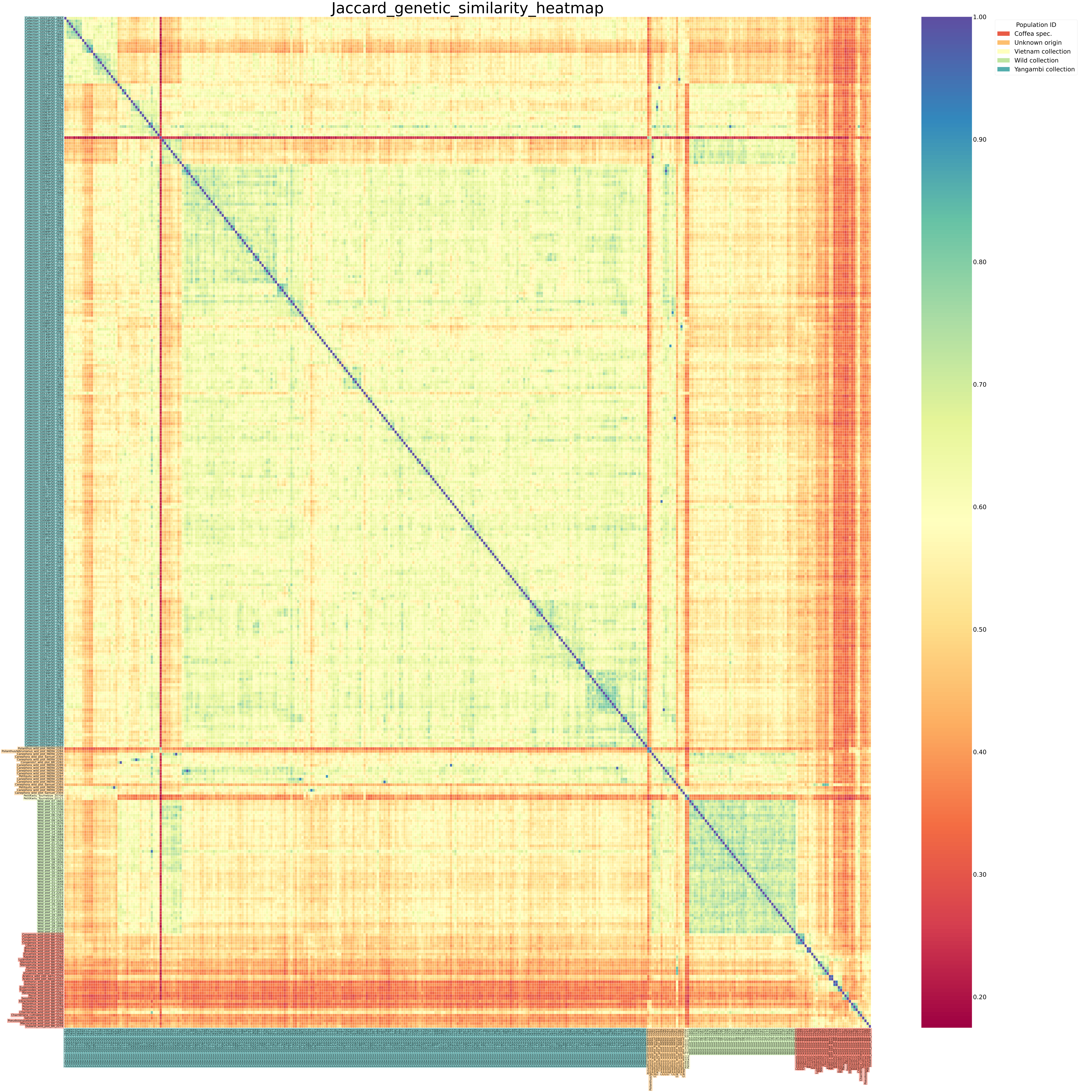
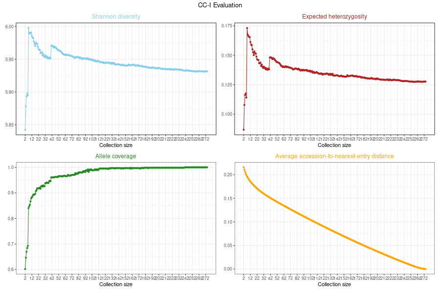
We chose the collection size corresponding to the local Shannon diversity and expected heterozygosity peak around size 40. We determined this peak is present at size 42 by looking at the values in the data frame.
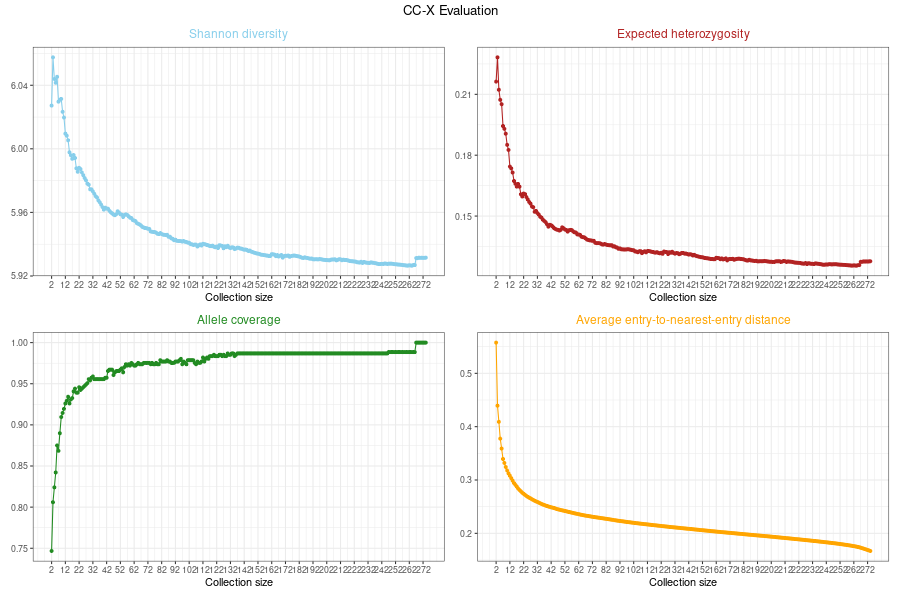
The CC-X collection size should be smaller than CC-I because CC-X contains collection extremes. We set a minimal allele coverage threshold of 95% for the collection because we also don’t want to lose too much genetic information. The smallest collection size that meets this criterion is 28.
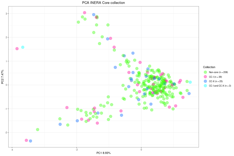
Using the sampleCore function of Core Hunter we selected the most suitable samples for each core collection strategy and visualized them in the PCA scatterplot. The optimal core size for both core collection strategies is also stated in the legend. The samples assigned to both CC-I and CC-X core collection were evenly distributed across the ordination space of the Yangambi coffee collection. Only 3 samples are present in both CC-I and CC-X collections.
Population genetics of bullfrog, an invasive species
This study involves several hunderd diploid individuals, sampled from 38 locations. Each individual was genotyped using double-digest GBS (PstI-EcoRI). These populations were sampled in Belgium, where bullfrog is an invasive species. The purpose of the study is to analyse population structure and relate this to geographical spread of the species.
GBprocesS
Demultiplexing was done using GBprocesS. See instruction for download and installation of GBprocesS. This is the config (.ini) file used for demultiplexing, trimming, merging forward and reverse reads, base quality filtering, and finaly removal of reads with internal restriction sites. Note that library preparation for such very large sample sets is usually done in several batches, whereby each batch reuses the sample-specific barcodes in the barcode adapter, and each batch is amplified with different sets of i5 and i7 Illumina barcodes during the PCR that adds the flowcell binding sites. In case some of the batch does not use all barcodes, it is important to include a “dummy” barcode in the demultiplexing (with non-existing sequence and the maximum length barcode used across the sample set). This is to make sure that all reads of each sample are trimmed to the same maximal length in the demultiplexing step. This is an example for a barcode file for demultiplexing of incomplete plates. For further explanation see the manual of GBprocesS.
Mapping reads with BWA-MEM
After demultiplexing and merging reads, they can be directly mapped onto a reference genome sequence. Here, we use the publicly available reference genome of bullfrog.
Prepare the reference genome and index it:
BWA
Map the reads of all samples onto the reference genome:
BWA mem
SMAP delineate
A first quality control of any GBS experiment is to run SMAP delineate on the BAM files of the entire sample set.
SMAP delineate:
smap delineate $download_dir/Real_data/SMAP_delineate/input/ind/ -mapping_orientation ignore --processes 8 --plot all --plot_type pdf --min_stack_depth 2 --max_stack_depth 1500 --min_cluster_length 50 --max_cluster_length 300 --max_stack_number 20 --min_stack_depth_fraction 10 --min_cluster_depth 10 --max_cluster_depth 1500 --max_smap_number 20 --name 48_ind_GBS-PE
SMAP delineate will provide an overview of the read mapping quality, locus length distribution, locus read depth distribution, the number of loci per sample (saturation curve) and locus completeness across the sample set.
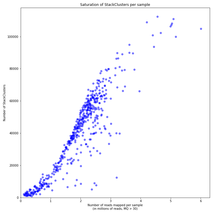
In this case (as shown by the saturation curve), the normalisation of the sample set was not optimal. Almost none of the samples reached locus saturation, with more than 100.000 loci detected for the samples with the largest library size (5-6M reads mapped). This can be explained by the large genome size of the species (about 3 Gb). Most of the samples are positioned on the steep part of the saturation curve (2-3M reads, 40-60k loci), meaning they have insuffcient reads to cover all possible loci with minimal read depth (here RD 15), and sequencing deeper would have yielded more loci per sample. This relatively high level of missing data (due to technical reasons) affects the possibility to compare samples by “common loci”. In addition, some of the samples have nearly no reads (100-500k reads) and a very minimal number of detected loci and are ‘dropout’ samples. The question, then, is how to set a threshold for minimal library size to retain good quality samples?
Effect of library size on genetic relationship estimations
To estimate the number of reads required per sample to estimate stable genomic fingerprints and to quantitatively estimate population genetics parameters, we first investigate how library size affects estimation of genetic relatedness. For this, we chose 14 samples with very high library size (4-6M merged reads after demultiplexing) representing different sampling locations.
we quickly checked (with SMAP haplotype-window and SMAP relatedness) that these samples indeed represent the genetic diversity (range 0.7-1.0) across the sample set (sneak preview of the rest of the analysis).
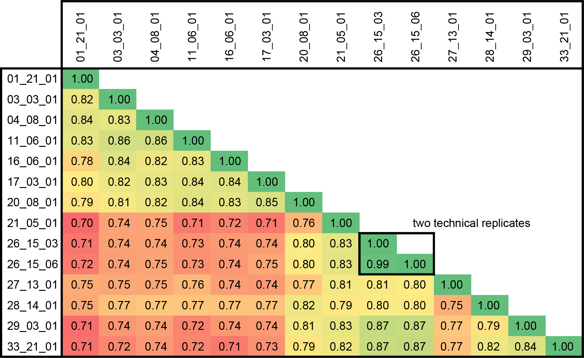
We then created ‘saturation’ curves that show how many reads are required per sample to yield a given number of loci. Furthermore, we analysed how a reduced number of loci affects pairwise genetic relationship estimation (using SMAP delineate, SNP calling with SAMtools, SMAP haplotype-sites and finally SMAP relatedness). The purpose of this step is to estimate the minimum number of reads required per sample, and conversely, to select samples with at least that number of reads for the rest of the analysis. Other samples with lower number of reads are excluded, as they have too little data to yield good quality genetic fingerprints.
We created a series of simulated incomplete samples by computationally subsampling the .fastq files:
head -n 400000 01_21_01.fq > 01_21_01_0.10.fq
head -n 800000 01_21_01.fq > 01_21_01_0.20.fq
head -n 1200000 01_21_01.fq > 01_21_01_0.30.fq
head -n 1600000 01_21_01.fq > 01_21_01_0.40.fq
head -n 2000000 01_21_01.fq > 01_21_01_0.50.fq
head -n 3000000 01_21_01.fq > 01_21_01_0.75.fq
head -n 4000000 01_21_01.fq > 01_21_01_1.00.fq
head -n 5000000 01_21_01.fq > 01_21_01_1.25.fq
head -n 6000000 01_21_01.fq > 01_21_01_1.50.fq
head -n 7000000 01_21_01.fq > 01_21_01_1.75.fq
head -n 8000000 01_21_01.fq > 01_21_01_2.00.fq
head -n 9000000 01_21_01.fq > 01_21_01_2.25.fq
head -n 10000000 01_21_01.fq > 01_21_01_2.50.fq
head -n 11000000 01_21_01.fq > 01_21_01_2.75.fq
head -n 12000000 01_21_01.fq > 01_21_01_3.00.fq
Here, the name of the files is coded as follows (split by '_'): first code indicates the location, the second code the individual, the third the replicate. numbers at the end of the file indicate the number of reads included after subsampling (in M) to simulate incomplete data.
This code is repeated for each of 14 samples (.fastq files).
We then ran SMAP delineate again to create the corresponding saturation curve:
smap delineate $download_dir/Real_data/SMAP_delineate/input/ind/ -mapping_orientation ignore --processes 8 --plot all --plot_type pdf --min_stack_depth 2 --max_stack_depth 1500 --min_cluster_length 50 --max_cluster_length 300 --max_stack_number 20 --min_stack_depth_fraction 10 --min_cluster_depth 10 --max_cluster_depth 1500 --max_smap_number 20 --name 48_ind_GBS-PE
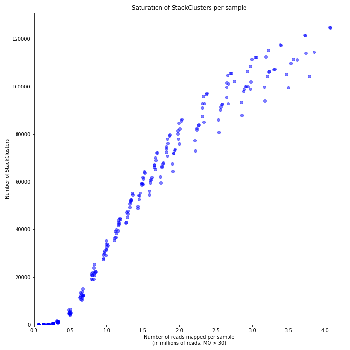
This curve indeed shows that the shape of the locus saturation curve observed for the entire sample set can be expained by suboptimal library size of a substantial number of samples.
Next, we ran SAMtools to identify SNPs in the 14 samples with complete data:
samtools
We used the .bed file with locus coordinates created by SMAP delineate to select 5000 loci with 2 SMAPs and completeness across all 14 samples. Running SAMtools on this locus set ensures that there is data in all 14 samples, and that in principle all pairwise comparisons to the “ground truth” can be made (as the ground truthh is based on “complete data”). Samtools identified 4000 SNPs in about 2500 loci.
Then, we ran SMAP haplotype-sites to create haplotype tables, and ran SMAP relatedness pairwise to estimate genetic relatedness (Jaccard similarity of loci with partially shared alleles):
smap haplotype-sites
smap relatedness pairwise
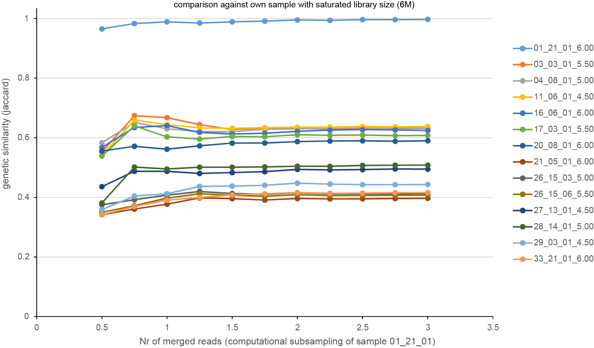
This shows that the estimated genetic relatedness is stable from 1 - 1.25M or more merged reads. With less read data, the estimation of genetic fingerprints starts to deviate from the ground truth (compared to its own sample with saturated data, value expected to be 1.00).
Selection of good quality samples
Now that we have estimated that using samples with at least 1M merged reads is required for good quality population genetic analysis, we will only continue with those 455 samples. These are distributed across the 38 locations as follows.
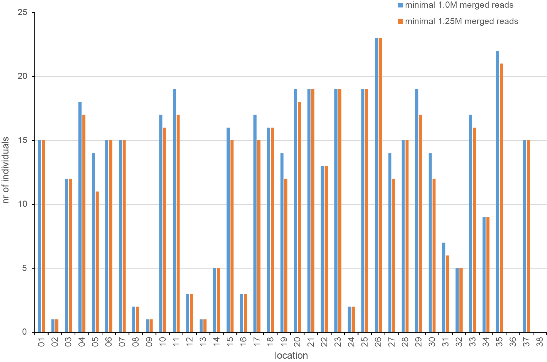
We next run SMAP delineate again to estimate the completeness and saturation of this sample set.
SMAP delineate:
smap delineate $download_dir/Real_data/SMAP_delineate/input/ind/ -mapping_orientation ignore --processes 8 --plot all --plot_type pdf --min_stack_depth 2 --max_stack_depth 1500 --min_cluster_length 50 --max_cluster_length 300 --max_stack_number 20 --min_stack_depth_fraction 10 --min_cluster_depth 10 --max_cluster_depth 1500 --max_smap_number 20 --name 48_ind_GBS-PE
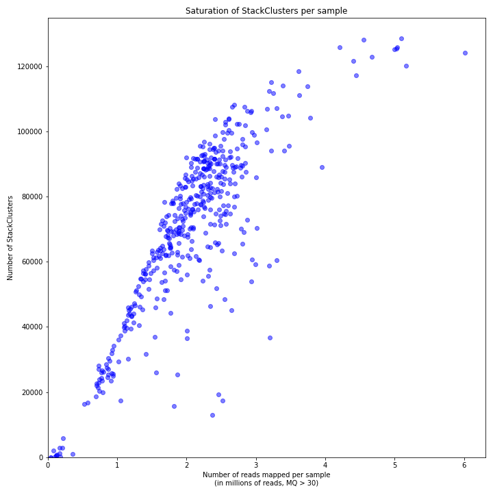
Identify SNPs
Instructions to identify and filter SNPs
SMAP haplotype-sites
Create and navigate to a new output directory to run SMAP haplotype-sites on the BAM files with mapped GBS reads of a set of individuals, its BED file from SMAP delineate, and a VCF file with SNP calls (see for third-party SNP calling software: e.g. SAMtools, BEDtools, Freebayes, or GATK for individuals):
mkdir -p $download_dir/Real_data/SMAP_haplotype_sites/output/ind
cd $download_dir/Real_data/SMAP_haplotype_sites/output/ind
smap haplotype-sites $download_dir/Real_data/SMAP_delineate/input/ind/ $download_dir/Real_data/SMAP_delineate/output/ind/final_stack_positions_48_ind_GBS-PE_C0_SMAP20_CL50_300.bed $download_dir/Real_data/SMAP_haplotype_sites/input/48_ind_GBS-PE.vcf --out haplotypes_48_ind_GBS-PE -mapping_orientation ignore --discrete_calls dosage --frequency_interval_bounds diploid --dosage_filter 2 --plot all --plot_type pdf -partial include --min_distinct_haplotypes 2 --min_read_count 10 --min_haplotype_frequency 5 --processes 8