Examples

Illustration of read mapping distribution in succesful GBS data

Below, we present six good quality GBS data sets analysed with SMAP delineate to illustrate typically expected read mapping distributions. For each data set, the command to run SMAP delineate with suggested optimal settings, together with graphical results are displayed for comparison to your own data.

Please note that while we suggest ‘optimal’ parameter settings in the command to run SMAP delineate, the default of SMAP delineate is to perform as little filtering as possible and to report all loci. The user is adviced to run SMAP delineate first with the mandatory and default settings (no data filtered out), and then decide on the most optimal parameter settings for your own data. Parameter settings should be iteratively adjusted for each novel data set, after manual inspection of the graphical output. The example data shown below are merely meant to illustrate the expected outcome of data sets processed with parameters adjusted to the specific type of library, reads and samples. If your data does not look like these examples, please check out the section Recommendations and Troubleshooting for examples (and suggested solutions) of incorrectly generated, preprocessed, or mapped GBS reads, or sample sets analyzed with inappropriate parameter settings for SMAP delineate. There, some guidelines for troubleshooting are provided, which may help to optimize GBS library preparation, sequencing, read preprocessing or SMAP delineate parameter settings.

Tab command shows a typical command to run SMAP delineate for double-enzyme GBS, single-end reads in diploid individuals.

Tabs for subsequent steps of Stack delineation show typical graphical results together with explanation about step-specific parameters.

smap delineate /path/to/BAM/ -mapping_orientation stranded  -p 8 --plot all --plot_type png --name 2n_ind_GBS-SE -f 50 -g 200 --min_stack_depth 3 --max_stack_depth 500 --min_cluster_depth 10 --max_cluster_depth 1500 --max_stack_number 2 --min_stack_depth_fraction 10 --completeness 1 --max_smap_number 10
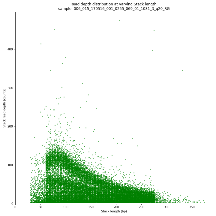
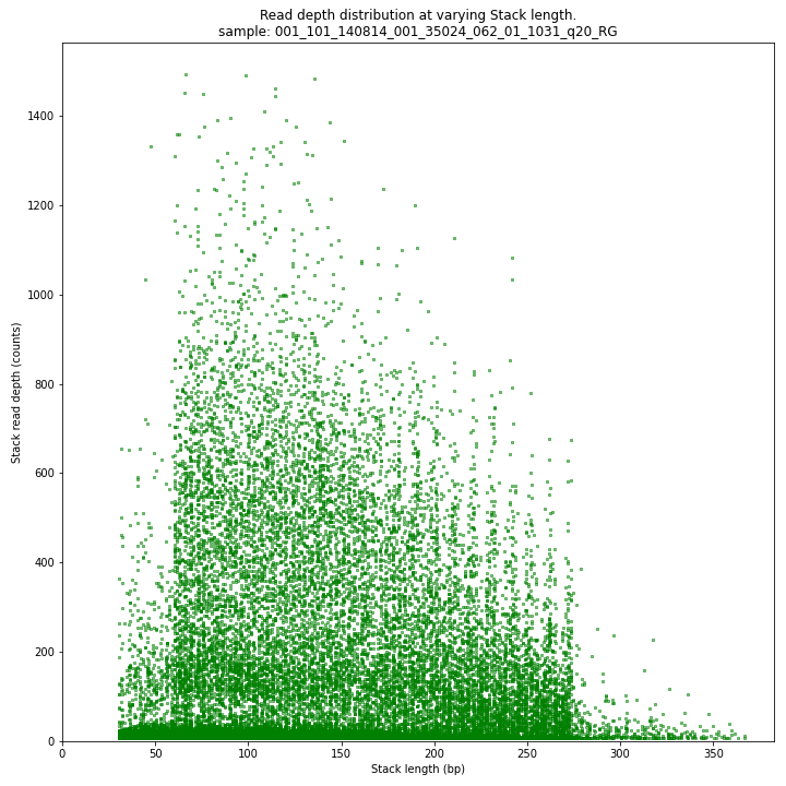
SMAP delineate run with --plot all plots the distribution of the length and read depth per Stack. Stacks are defined by read mapping start and end positions on the reference sequence, hence Stacks can be shorter or longer than the longest read length.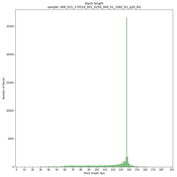

The majority of loci is expected to show Stack length (region covered by the mapped read) equal to maximal read length (in this case 136 bp, after barcode and RE trimming of a 150 bp read). Shorter Stacks are created when RE’s are closer to each other than the maximal sequencing length or when insertions occur. Longer Stacks are created when deletions occur. See section on InDels.

_________________________________________________________________________________________________

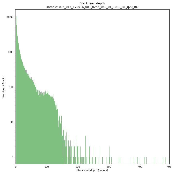
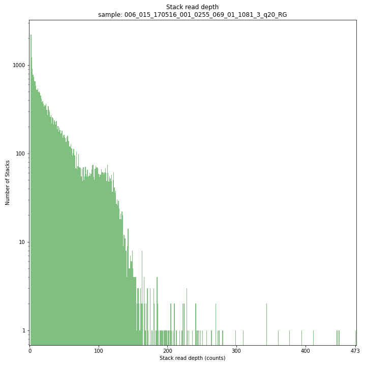
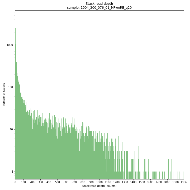
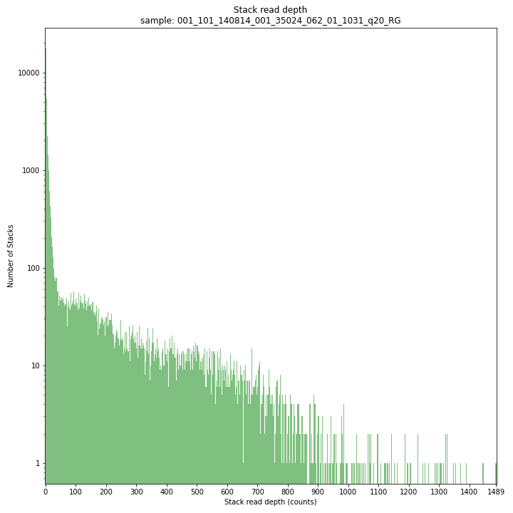
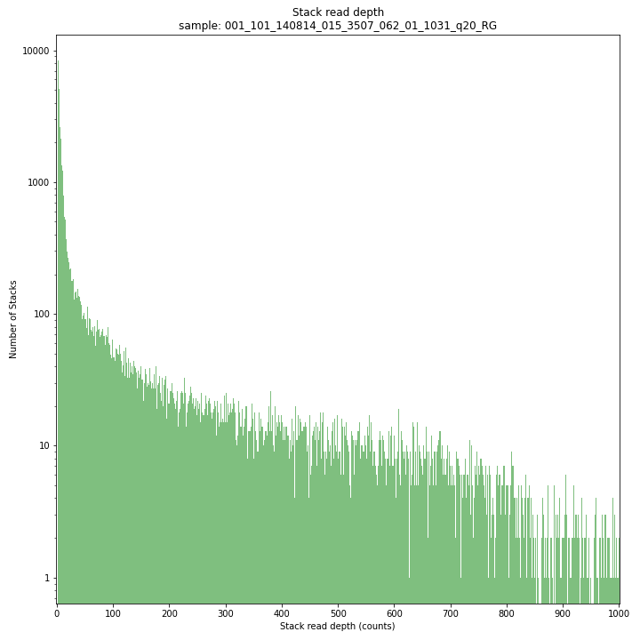
The Stack read depth distribution typically follows a left-skewed distribution, with many loci with relatively low read depth, and few loci at comparably high read depth. The shape of the read depth distribution results from differences in PCR-amplification and sequencing efficiency between GBS-fragments due to variation in fragment length, GC-content, and other factors. Loci with relatively high read depth are typically derived from repeat sequences that are mapped onto a single representative locus in the reference sequence.

_________________________________________________________________________________________________

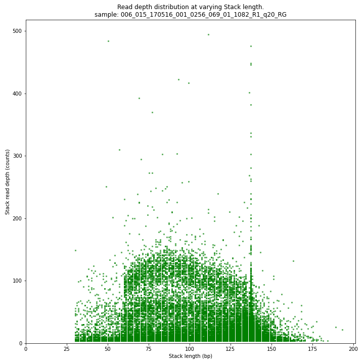
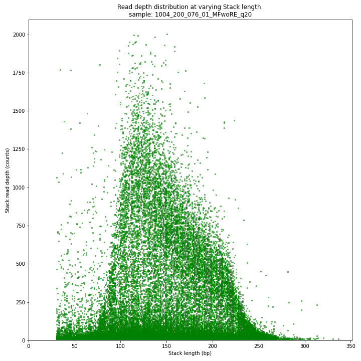
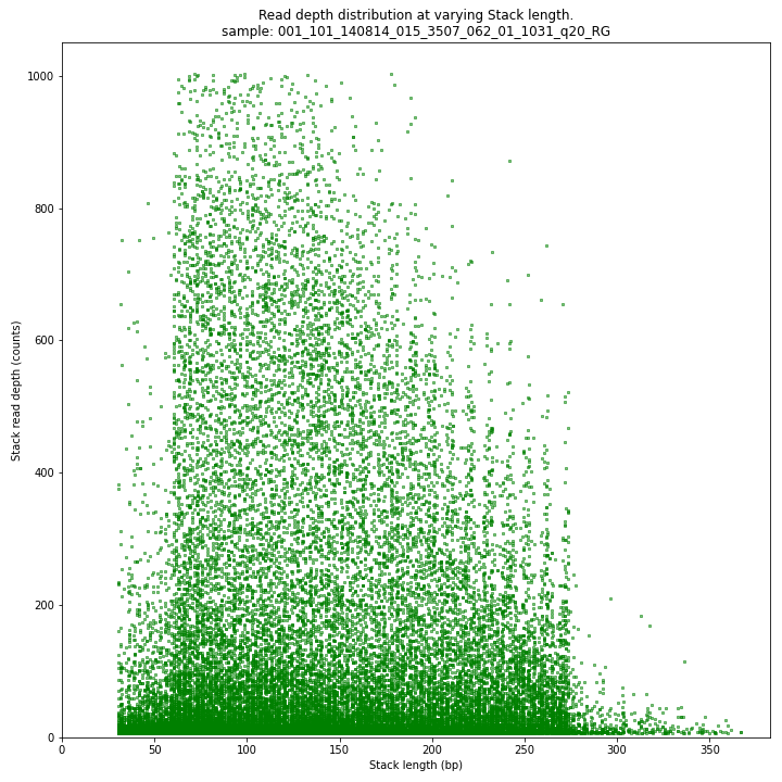
The Stack read depth and read length correlation distribution is expected to follow the Stack length distribution. It is recommended to not fill in the --max_stack_depth and --max_cluster_depth options (defaulting to infinite) during a trial run and to subsequently choose these values based on this (and the StackCluster.LengthDepthCorrelation scatter) plot. Extremely deeply sequenced loci are often short sequence repeats originitating from different loci on the genome but mapping on a single one.

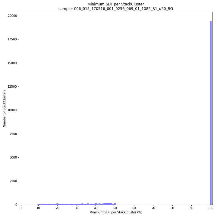
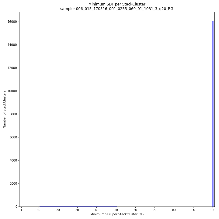
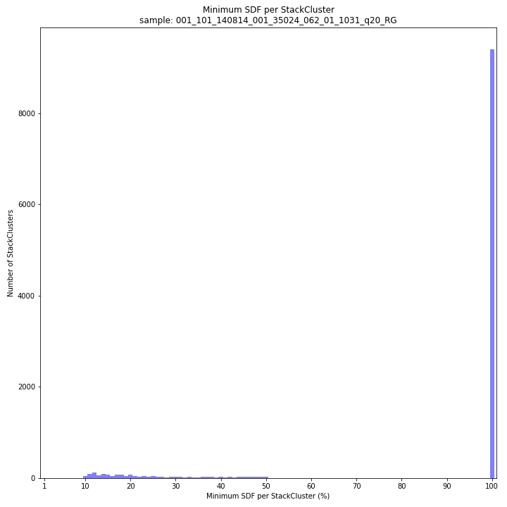
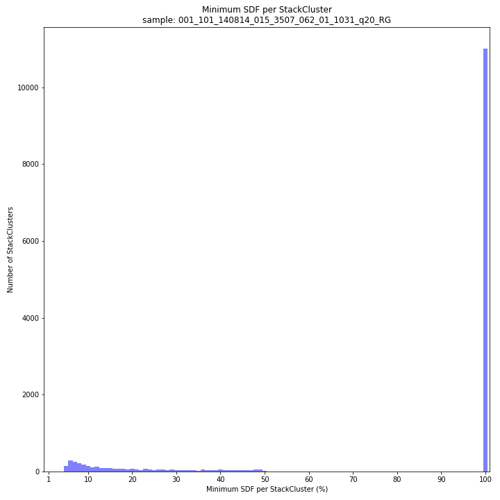
SMAP delineate run with --plot all plots the StackCluster mapping characteristics such as: the length, the read depth, the number of overlapping Stacks, and the Fraction of Stack read depth / total StackCluster read Depth (SDF).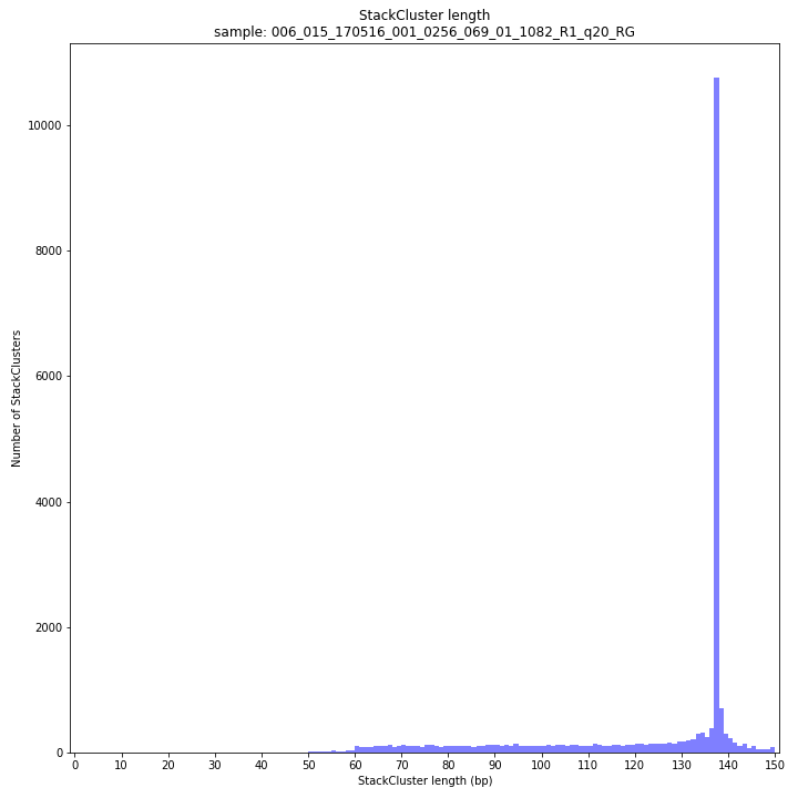

The majority of loci is expected to show StackCluster length similar to maximal read length (in this case 136 bp, after barcode and RE trimming of a 150 bp read). StackCluster length is defined by the outermost SMAPs after overlap of the underlying Stacks. Short Stacks can thus ‘hide’ under longer StackClusters, or two partially overlapping Stacks can increase total StackCluster length, slightly increasing the StackCluster length distribution compared to the Stack length distribution.

_________________________________________________________________________________________________

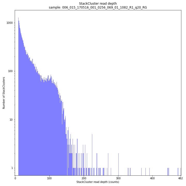
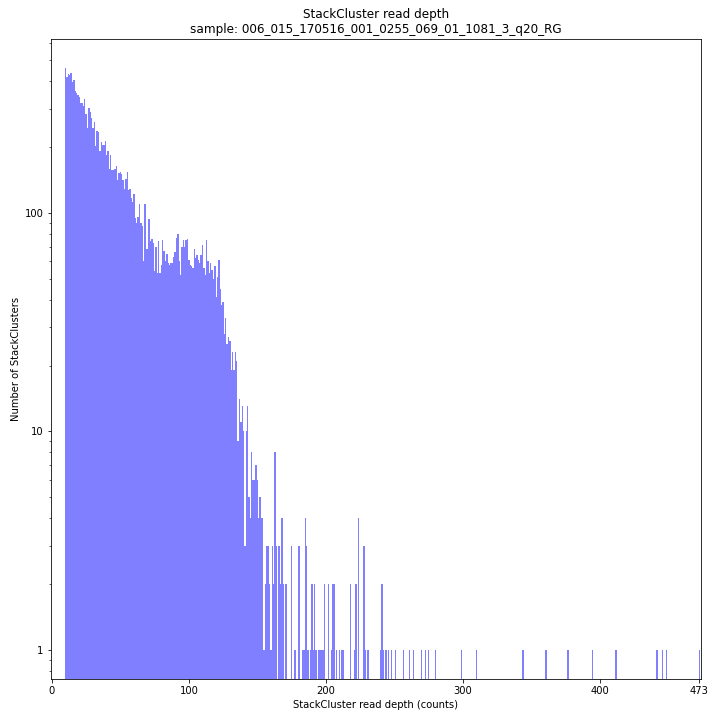
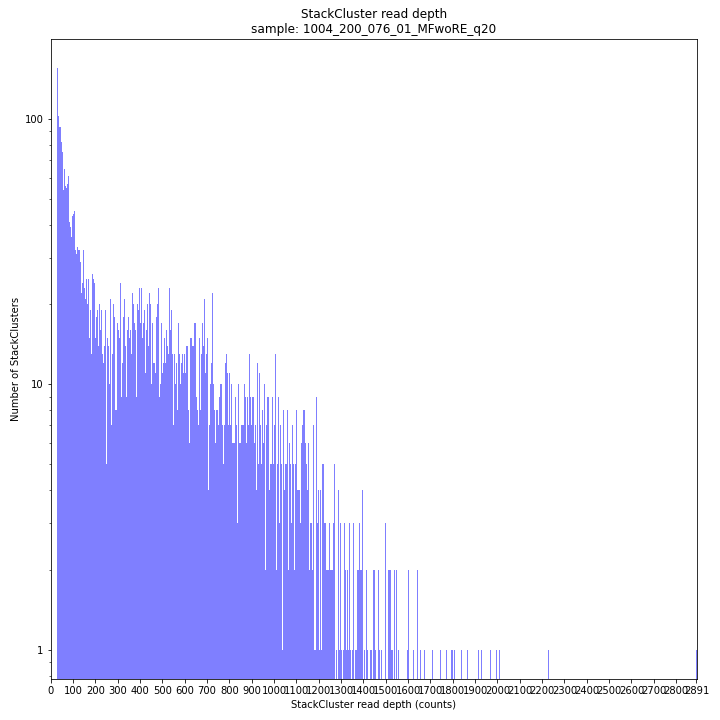
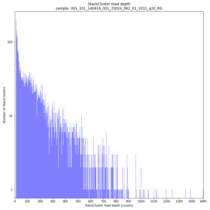
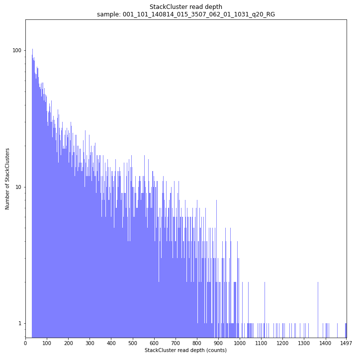
The StackCluster read depth distribution typically follows a left-skewed distribution, just like the Stack read depth distribution. Read depth values are slightly higher as StackClusters contain the sum of the underlying Stack read depths.

_________________________________________________________________________________________________

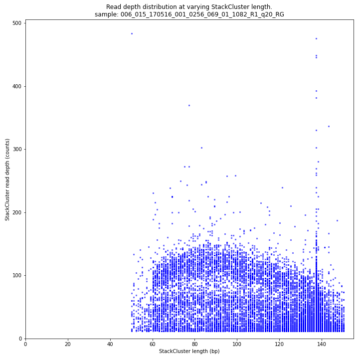
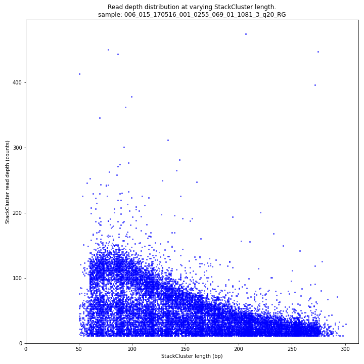
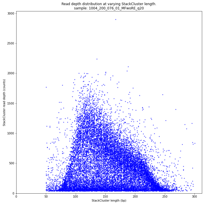
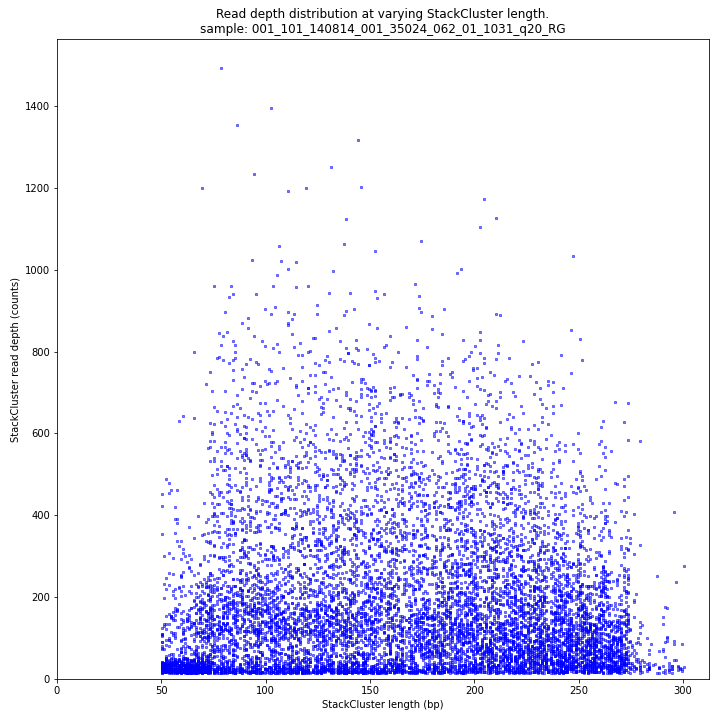
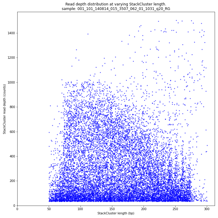
The StackCluster read depth and length correlation distribution is expected to follow the StackCluster length distribution. It is recommended to not fill in the --max_stack_depth and --max_cluster_depth options (defaulting to infinite) during a trial run and to subsequently choose these values based on this (and the Stack.LengthDepthCorrelation scatter) plot. Extremely deeply sequenced loci are often short sequence repeats originitating from different loci on the genome but mapping on a single one.

_________________________________________________________________________________________________

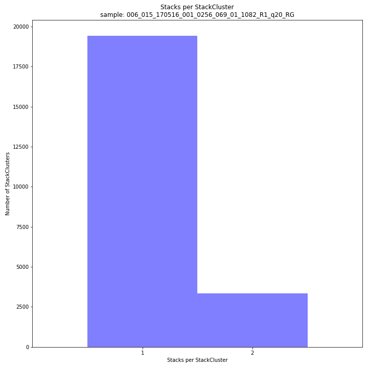
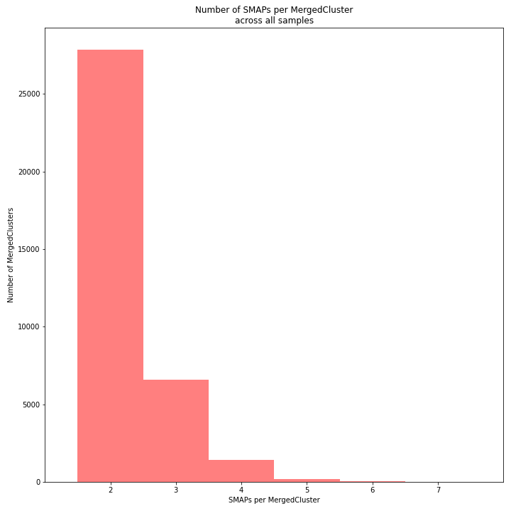
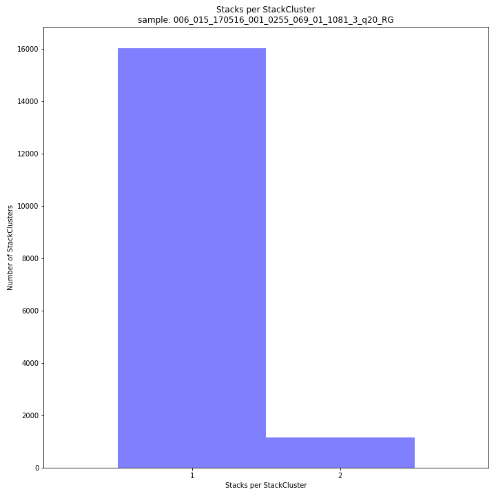
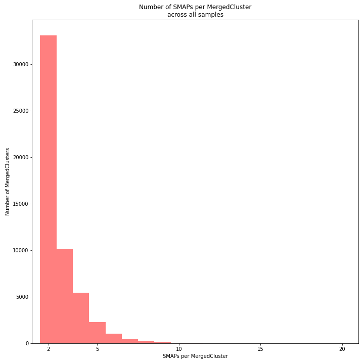
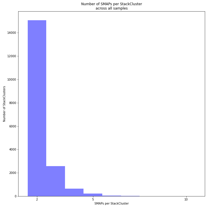
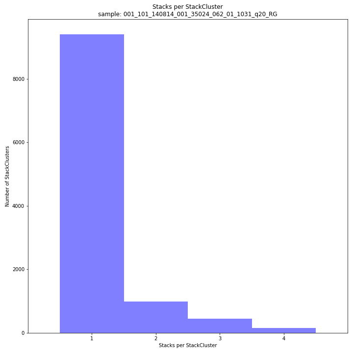
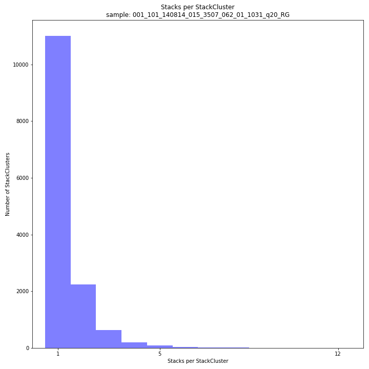
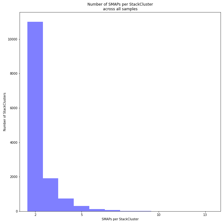
The distribution of the number of Stacks per StackCluster across all loci per sample indicates the abundance of read mapping polymorphisms in the GBS data. By definition, in diploids, a StackCluster can contain 1 or 2 Stacks which are then delineated by 2 or 3 and 4 SMAPs, respectively (see scheme below). StackClusters with excess numbers of Stacks can be removed using the option -l or --max_stack_number. For diploid individuals, the recommended value for this option is 2.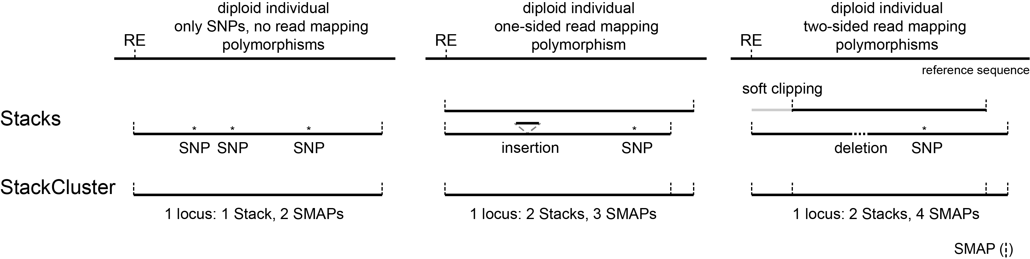

_________________________________________________________________________________________________

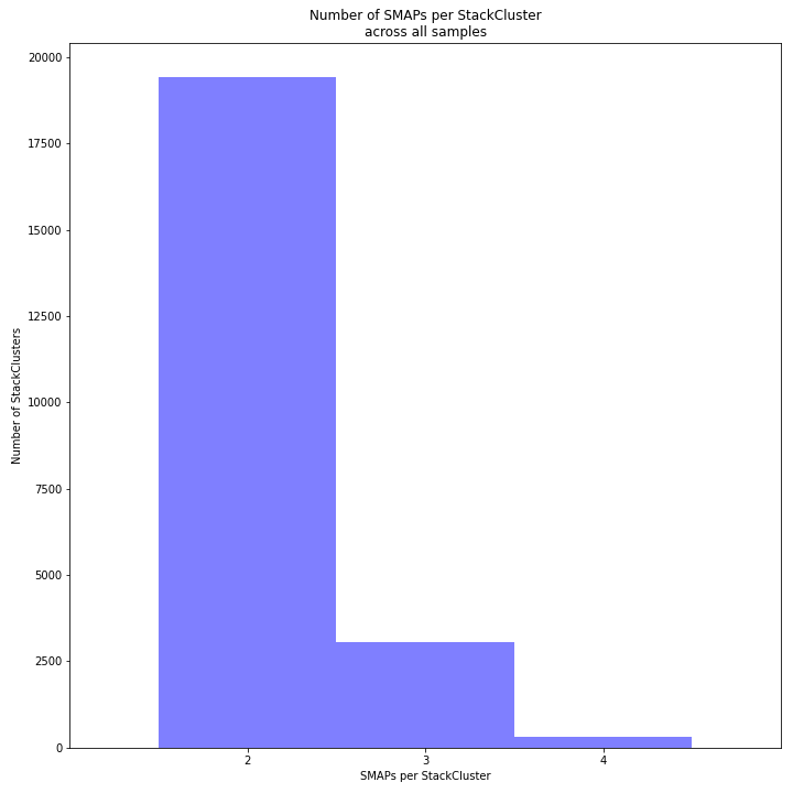
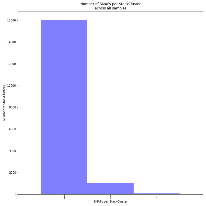
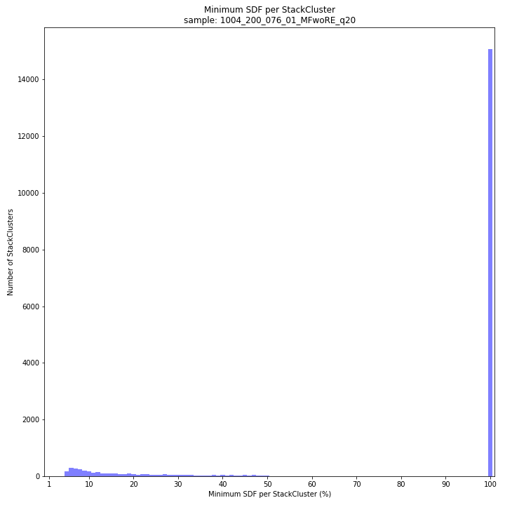
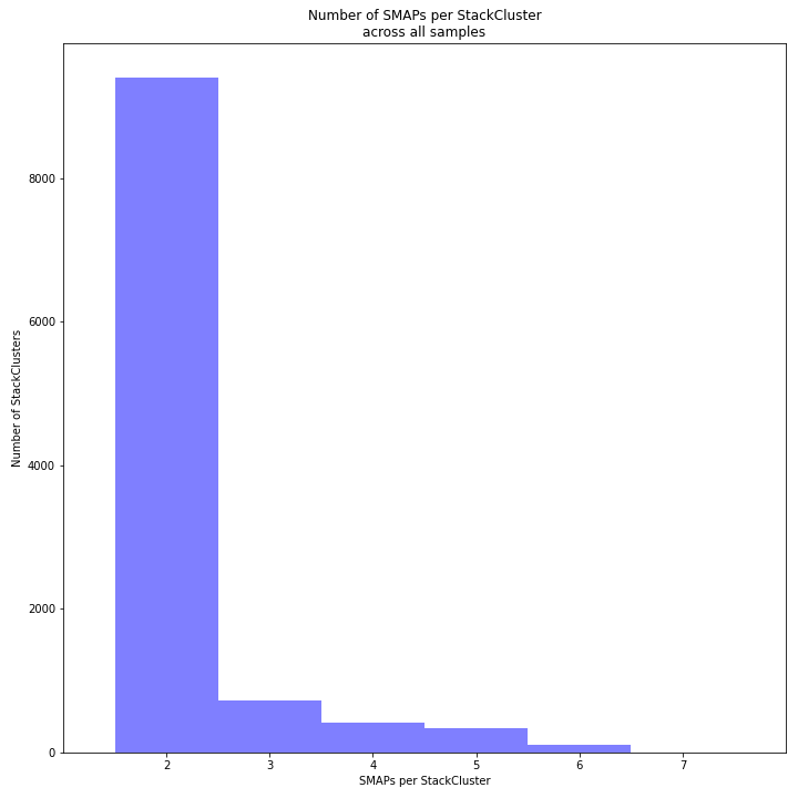
The image above depicts the number of SMAPs per StackCluster. By definition, 2 SMAPs result in either a single Stack or 2 Stacks without length polymorphisms but with SNPs. In diploids, the maximum number of SMAPs per StackCluster is 4; 2 Stacks with different start and stop positions. This situation is rare and the majority of StackClusters are expected to contain 2 or 3 SMAPs. StackClusters with excess Stacks (incorporation of SMAPs and SNPs) can be removed using the option -l or --max_stack_number, for diploids the recommended value for this option is 2.

_________________________________________________________________________________________________

text

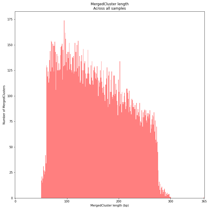
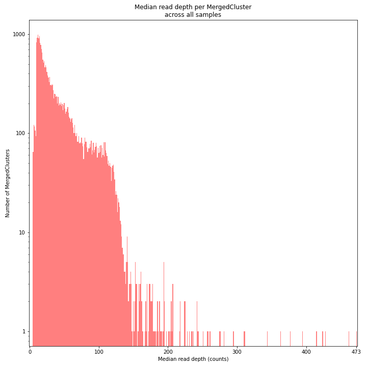
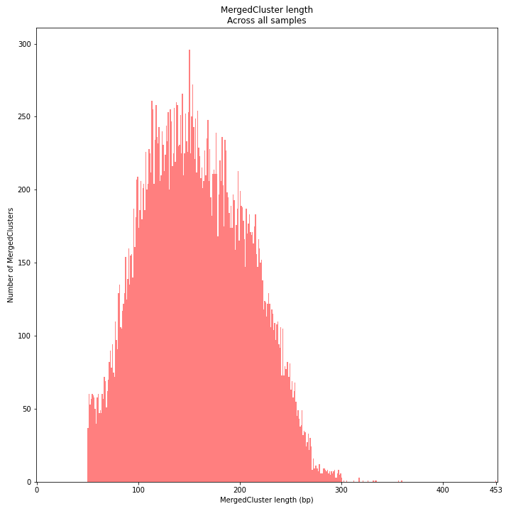
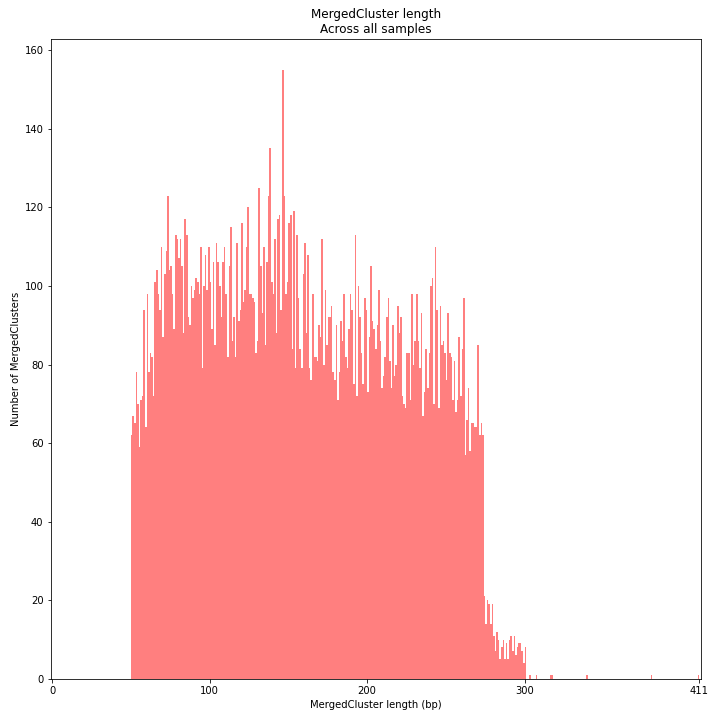
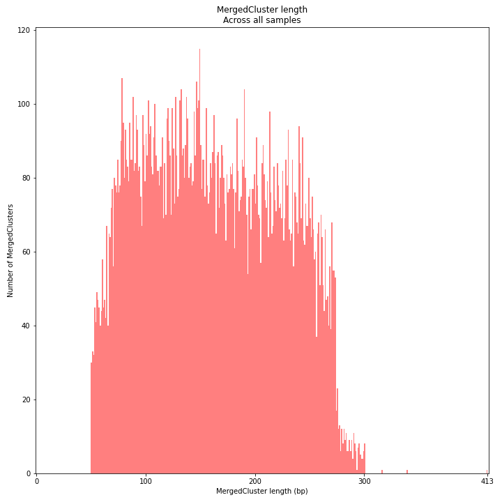
SMAP delineate by default plots the MergedCluster mapping characteristics such as: length, median read depth, number of overlapping SMAPs per MergedCluster, number of samples that contribute to a MergedCluster (Completeness).

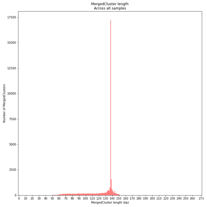
MergedCluster length is defined by the outermost SMAPs after overlap of all StackClusters per locus across all samples. The MergedCluster length distribution is expected to be similar or slightly longer compared to the StackCluster length distribution, but a clear single peak is expected at the maximum read length. High between-sample genetic variation in the sample set is expected to increase MergedCluster length compared to StackCluster length.

_________________________________________________________________________________________________

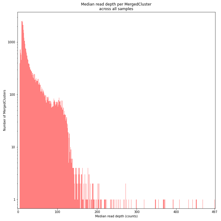
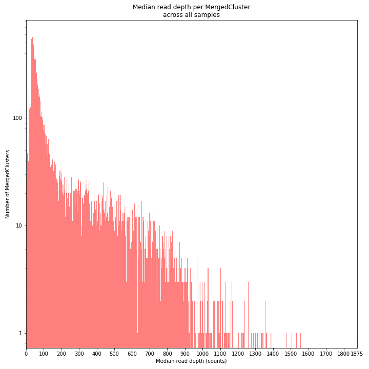
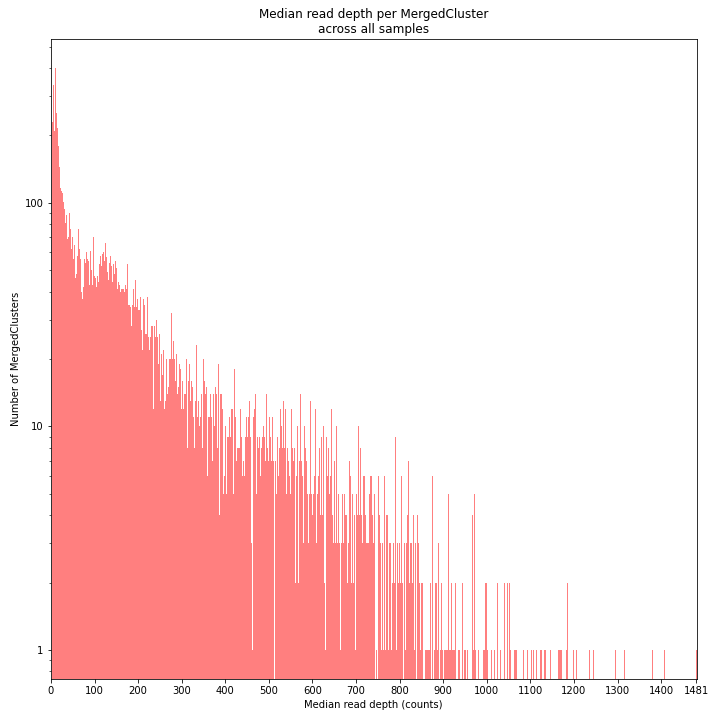
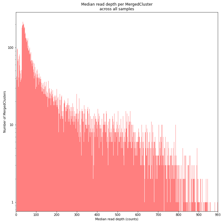
The median MergedCluster read depth distribution is a combination of the different StackCluster distributions. It gives an idea of how many loci are shared between at least half of the samples at at least a given read depth. The more similar this distribution is to each individual StackCluster read depth plot, the more complete the data are.

_________________________________________________________________________________________________

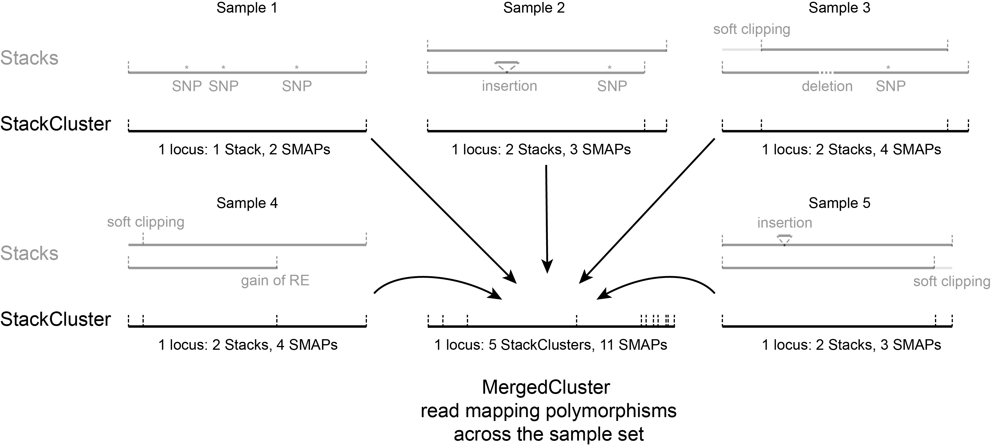
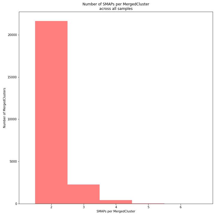
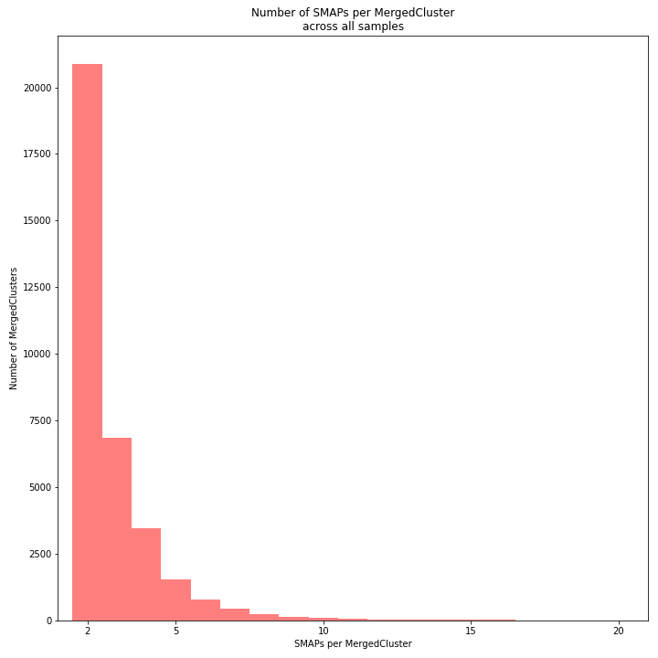
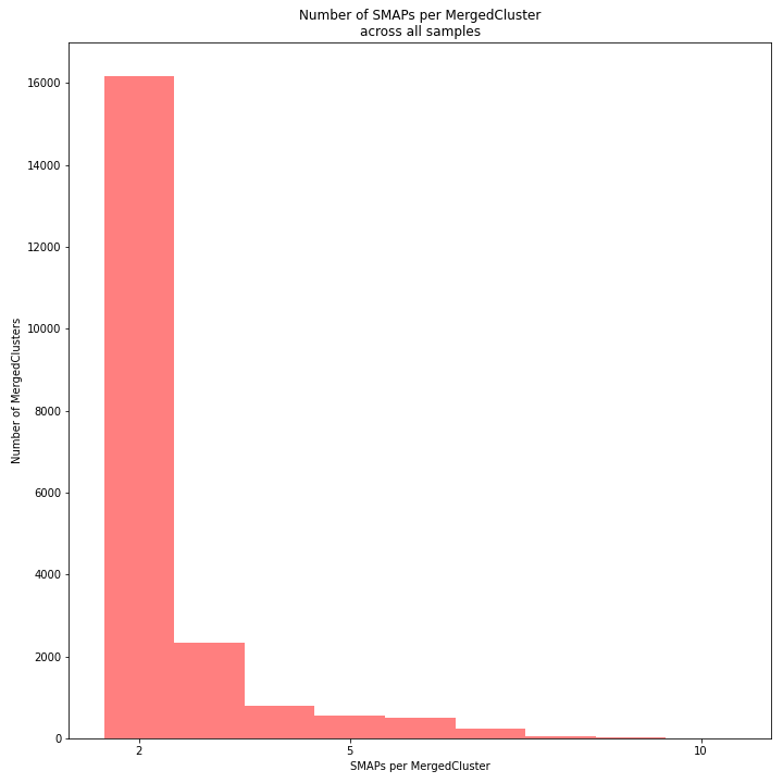
The distribution of the number of SMAPs per locus shows the abundance of read mapping polymorphisms across the sample set. This distribution is key to evaluating if it is crucial in your sample set to take read mapping polymorphisms into account. The majority of MergedClusters usually contain 2 SMAPs; in these loci, all reads per locus in the sample set have the same read mapping start and end positions. Loci with increasing numbers of SMAPs across the sample set are usually less abundant. The frequency of InDels and SNPs (causing alternative SMAPs) across the sample set is expected to be proportional to the genetic diversity displayed in read mapping polymorphisms (i.e. numbers of SMAPs per MergedCluster, see scheme below). Please note that technical artefacts, such as incorrect read trimming, also contribute to alternative read mapping polymorphisms across the sample set, and should be eliminated to avoid mistaking that as biological genetic diversity. See the section Recommendations and Troubleshooting for more details.

_________________________________________________________________________________________________

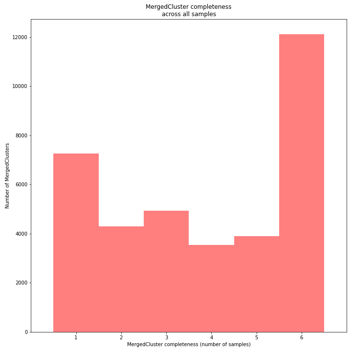
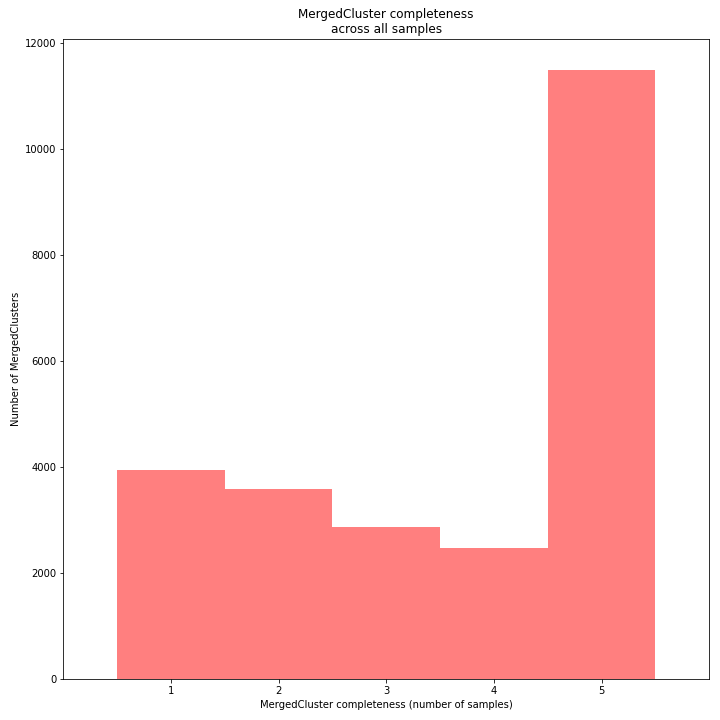
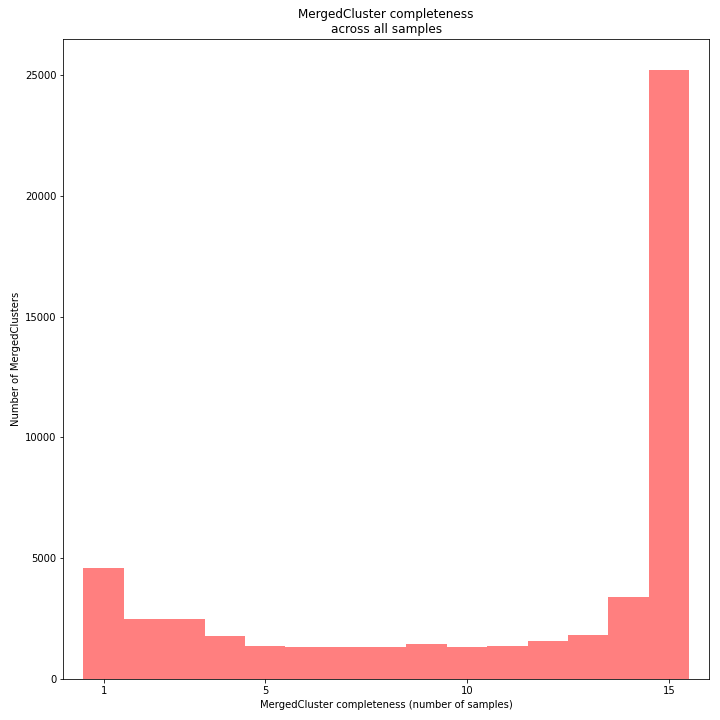
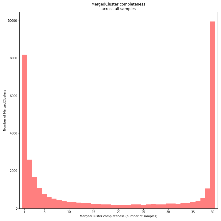
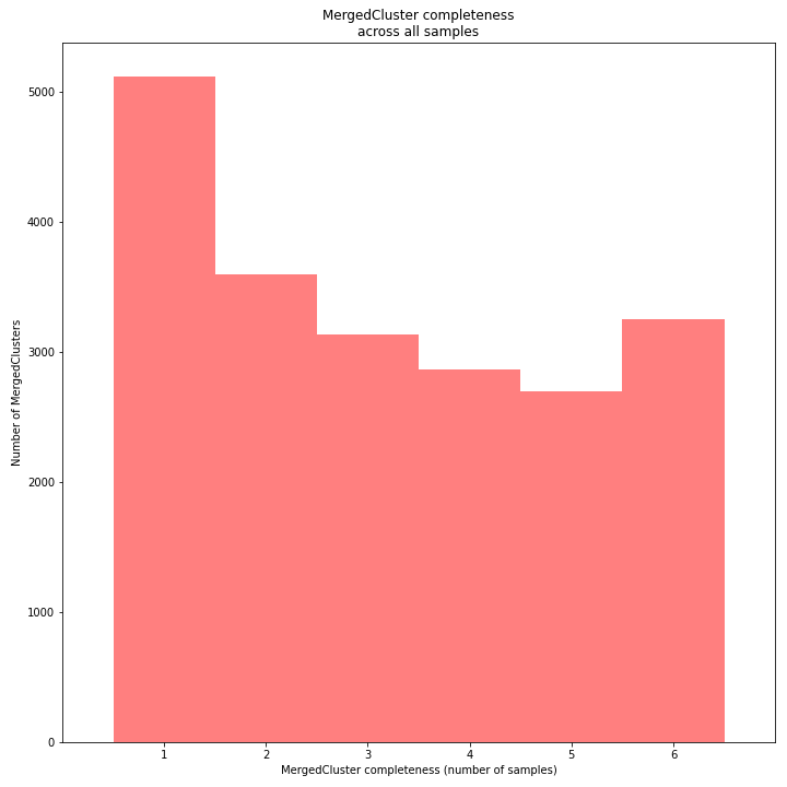
The distribution of completeness scores per MergedCluster across the sample set shows the fraction of the loci that have sufficient read depth in only a few samples (left side, lower completeness), and the fraction of loci that is commonly detected across the sample set (right side, higher completeness). This distribution is key to predicting missingness in the genotype calling table (sample-genotype matrix) for the sample set after downstream analysis. Each sample may have a similar total number of GBS loci (see read depth vs StackCluster saturation curve), but a small fraction may be shared across samples. The higher the genetic diversity across the sample set, the higher the number of sample-specific unique alleles and loci, the more left-skew in the completeness distribution, the lower the number of shared loci, and the more the total number of loci across the entire sample set is inflated.

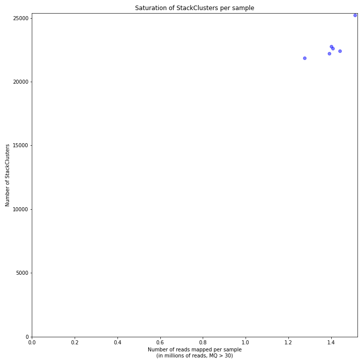
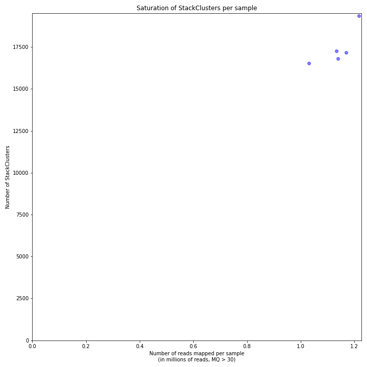
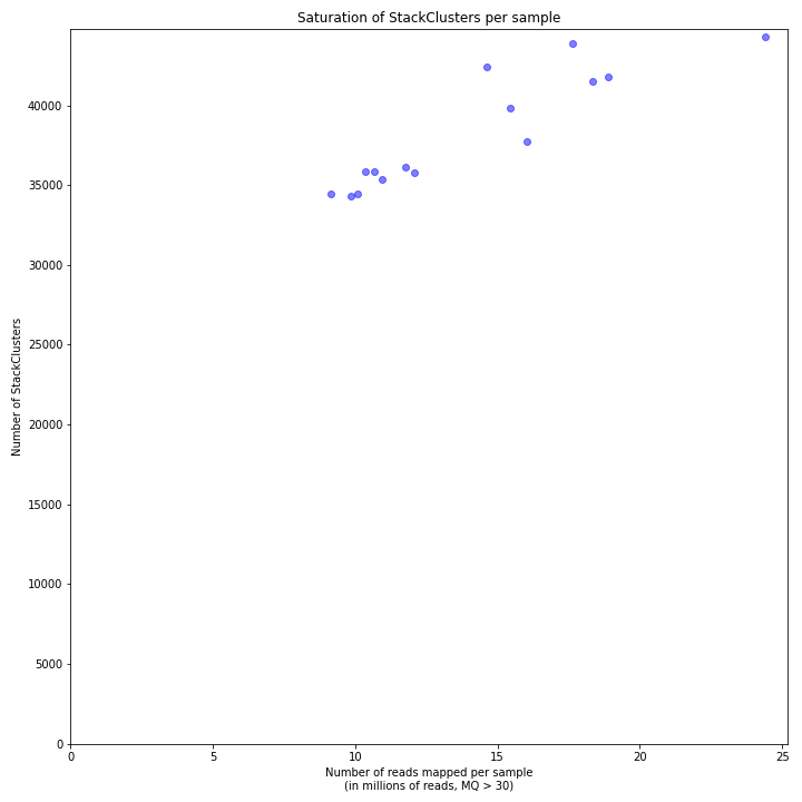
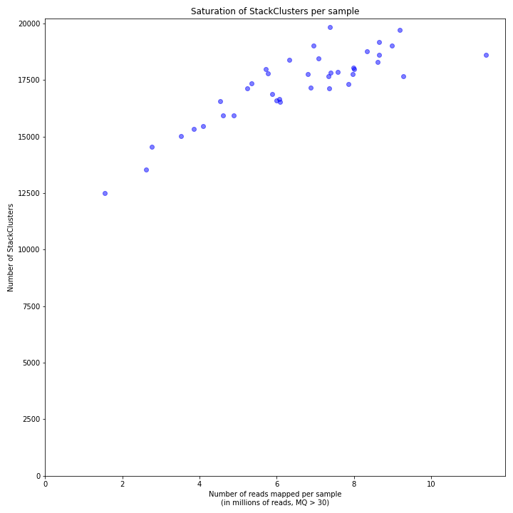
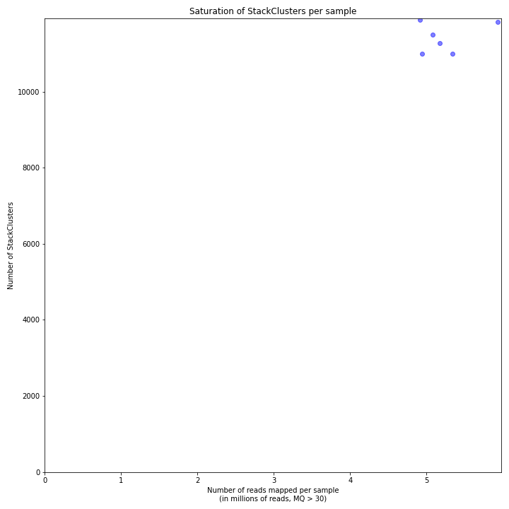
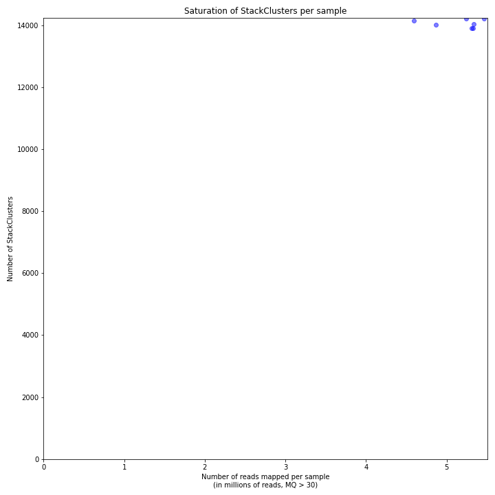
The saturation curve shows if the total number of reads obtained per sample leads to the maximum number of detected StacksClusters per sample. Each circle in the graph is a single sample.

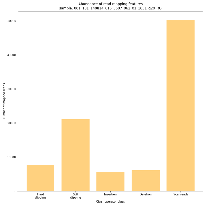
SMAP delineate run with --plot all plots the abundance of special features in the reference-read alignment (scored as Cigar strings). This graph shows the number of reads that include at least one occurence of H (hard clipping), S (soft clipping), D (deletion) or I (insertion), compared to the total number of reads in the BAM file. This abundance profile is a predictor for the number of expected read mapping polymorphisms, and should be in line with the distribution of the number of Stacks and SMAPs per StackCluster (per sample), and the number of SMAPs per MergedCluster (across the sample set).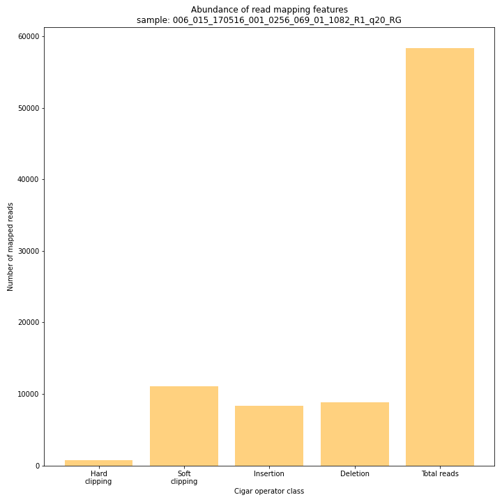

Tab command shows a typical command to run SMAP delineate for double-enzyme GBS, merged reads in diploid individuals.

Tabs for subsequent steps of Stack delineation show typical graphical results together with explanation about step-specific parameters.

smap delineate /path/to/BAM/ -mapping_orientation ignore -p 8 --plot all --plot_type png --name 2n_ind_GBS-PE -f 50 -g 300 --min_stack_depth 2 --max_stack_depth 500 --min_cluster_depth 10 --max_cluster_depth 1500 --max_stack_number 2 --min_stack_depth_fraction 10 --completeness 1 --max_smap_number 10
SMAP delineate run with --plot all plots the distribution of the length and read depth per Stack. Stacks are defined by start and end positions on the reference sequence, hence stacks can be shorter or longer than the longest read length.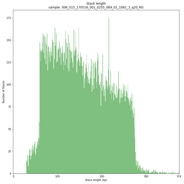

These merged reads were constructed from 136 bp each paired-end reads. Therefore with a minimum merging overlap of 10, the maximum merged read length becomes 262 bp. Any Stack longer than this contains deletions which alter the start and end positions on the reference sequence. Of course a minimum overlap of 10 does not exclude larger overlaps, therefore it is possible to merge two short reads (e.g. 40 bp) with a complete overlap and obtain a 40 bp Stack. Moreover, there is a PCR and sequencing bias towards these short reads as they are amplified faster.

_________________________________________________________________________________________________

The Stack read depth distribution typically follows a left-skewed distribution, with many loci with relatively low read depth, and few loci at comparably high read depth. The shape of the read depth distribution results from differences in PCR-amplification and sequencing efficiency between GBS-fragments due to variation in fragment length, GC-content, and other factors. Loci with relatively high read depth are typically derived from repeat sequences that are mapped onto a single representative locus in the reference sequence.

_________________________________________________________________________________________________

The Stack read depth and read length correlation distribution is expected to follow the Stack length distribution. It is recommended to not fill in the --max_stack_depth and --max_cluster_depth options (defaulting to infinite) during a trial run and to subsequently choose these values based on this (and the StackCluster.LengthDepthCorrelation scatter) plot. Extremely deeply sequenced loci are often short sequence repeats originitating from different loci on the genome but mapping on a single one.

SMAP delineate run with --plot all plots the StackCluster mapping characteristics such as: the length, the read depth, the number of overlapping Stacks, and the Fraction of Stack read depth/total StackCluster read Depth (SDF).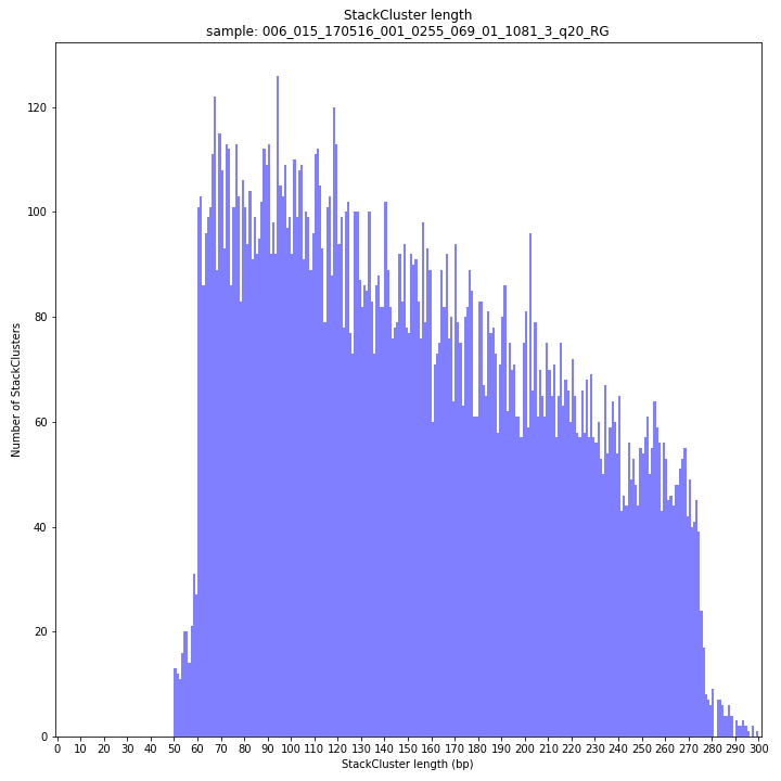

The majority of loci are expected to show a StackCluster length distribution (region covered by the Stacks) similar to the Stack length distribution, but shifted somewhat to the right. StackCluster length is defined by the outermost SMAPs after overlap of the underlying Stacks. Short Stacks can thus ‘hide’ under longer StackClusters, or two partially overlapping Stacks can increase total StackCluster length, slightly increasing the StackCluster length distribution compared to the Stack length distribution.

_________________________________________________________________________________________________

The StackCluster read depth distribution typically follows a left-skewed distribution, just like the Stack read depth distribution. Read depth values are slightly higher as StackClusters contain the sum of the underlying Stack read depths.

_________________________________________________________________________________________________

The StackCluster read depth and length correlation distribution is expected to follow the StackCluster length distribution. It is recommended to not fill in the --max_stack_depth and --max_cluster_depth options (defaulting to infinite) during a trial run and to subsequently choose these values based on this (and the Stack.LengthDepthCorrelation scatter) plot. Extremely deeply sequenced loci are often short sequence repeats originitating from different loci on the genome but mapping on a single one.

_________________________________________________________________________________________________

The distribution of the number of Stacks per StackCluster across all loci per sample indicates the abundance of read mapping polymorphisms in the GBS data. By definition, in diploids, a StackCluster can contain 1 or 2 Stacks which are then delineated by 2 or 3 and 4 SMAPs, respectively (see scheme below). StackClusters with excess numbers of Stacks can be removed using the option -l or --max_stack_number. For diploid individuals, the recommended value for this option is 2.

_________________________________________________________________________________________________

The image above depicts the number of SMAPs per StackCluster. By definition, 2 SMAPs result in either a single Stack or 2 Stacks without length polymorphisms but with SNPs. In diploids, the maximum number of SMAPs per StackCluster is 4; 2 Stacks with different start and stop positions. This situation is rare and the majority of StackClusters are expected to contain 2 or 3 SMAPs. StackClusters with excess Stacks (incorporation of SMAPs and SNPs) can be removed using the option -l or --max_stack_number, for diploids the recommended value for this option is 2.

_________________________________________________________________________________________________

text

SMAP delineate by default plots the MergedCluster mapping characteristics such as: Length, read depth, number of overlapping Stacks, number of Samples that contribute to a MergedCluster (Completeness).

MergedCluster length is defined by the outermost SMAPs after overlap of all StackClusters per locus across all samples. The MergedCluster length distribution is expected to be similar or slightly longer compared to the StackCluster length distribution, but a clear single peak is expected at the maximum read length. High between-sample genetic variation in the sample set is expected to increase MergedCluster length compared to StackCluster length.

_________________________________________________________________________________________________

The median MergedCluster read depth distribution is a combination of the different StackCluster distributions. It gives an idea of how many loci are shared between at least half of the samples at at least a given read depth. The more similar this distribution is to each individual StackCluster read depth plot, the more complete the data are.

_________________________________________________________________________________________________

The distribution of the number of SMAPs per locus shows the abundance of read mapping polymorphisms across the sample set. This distribution is key to evaluating if it is crucial in your sample set to take read mapping polymorphisms into account. The majority of MergedClusters usually contain 2 SMAPs; in these loci, all reads per locus in the sample set have the same read mapping start and end positions. Loci with increasing numbers of SMAPs across the sample set are usually less abundant. The frequency of InDels and SNPs (causing alternative SMAPs) across the sample set is expected to be proportional to the genetic diversity displayed in read mapping polymorphisms (i.e. numbers of SMAPs per MergedCluster, see scheme below). Please note that technical artefacts, such as incorrect read trimming, also contribute to alternative read mapping polymorphisms across the sample set, and should be eliminated to avoid mistaking that as biological genetic diversity. See the section Recommendations and Troubleshooting for more details.

_________________________________________________________________________________________________

The distribution of completeness scores per MergedCluster across the sample set shows the fraction of the loci that have sufficient read depth in only a few samples (left side, lower completeness), and the fraction of loci that is commonly detected across the sample set (right side, higher completeness). This distribution is key to predicting missingness in the genotype calling table (sample-genotype matrix) for the sample set after downstream analysis. Each sample may have a similar total number of GBS loci (see read depth vs StackCluster saturation curve), but a small fraction may be shared across samples. The higher the genetic diversity across the sample set, the higher the number of sample-specific unique alleles and loci, the more left-skew in the completeness distribution, the lower the number of shared loci, and the more the total number of loci across the entire sample set is inflated.

The saturation curve shows if the total number of reads obtained per sample leads to the maximum number of detected StacksClusters per sample. Each circle in the graph is a single sample.

SMAP delineate run with --plot all plots the abundance of special features in the reference-read alignment (scored as Cigar strings). This graph shows the number of reads that include at least one occurence of H (hard clipping), S (soft clipping), D (deletion) or I (insertion), compared to the total number of reads in the BAM file. This abundance profile is a predictor for the number of expected read mapping polymorphisms, and should be in line with the distribution of the number of Stacks and SMAPs per StackCluster (per sample), and the number of SMAPs per MergedCluster (across the sample set).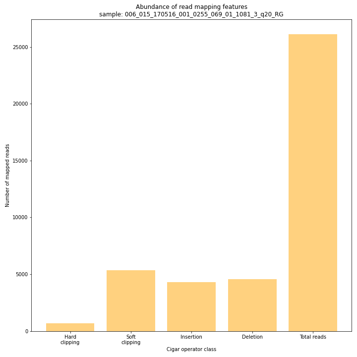

Tab command shows a typical command to run SMAP delineate for single-enzyme GBS, single-end reads in pools.

Tabs for subsequent steps of Stack delineation show typical graphical results together with explanation about step-specific parameters.

smap delineate /path/to/BAM/ -mapping_orientation stranded  -p 8 --plot all --plot_type png --name 2n_pools_GBS-SE -f 50 -g 150 --min_stack_depth 3 --max_stack_depth 1000 --min_cluster_depth 30 --max_cluster_depth 2000 --max_stack_number 10 --min_stack_depth_fraction 5 --completeness 1 --max_smap_number 20
SMAP delineate run with --plot all plots the distribution of the length and read depth per Stack. Stacks are defined by start and end positions on the reference sequence, hence stacks can be shorter or longer than the longest read length.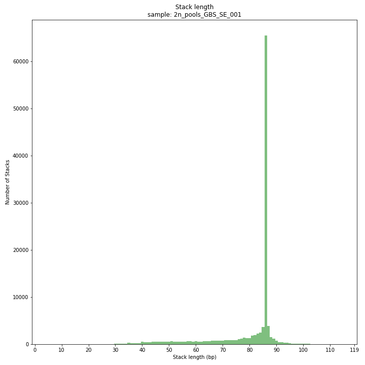

The majority of loci is expected to show Stack length (region covered by the mapped read) equal to maximal read length (in this case 86 bp, after barcode and RE trimming of a 100 bp read). Shorter Stacks are created when RE’s are closer to each other than the maximal sequencing length or when insertions occur. Longer Stacks are created when deletions occur. See section on InDels.

_________________________________________________________________________________________________

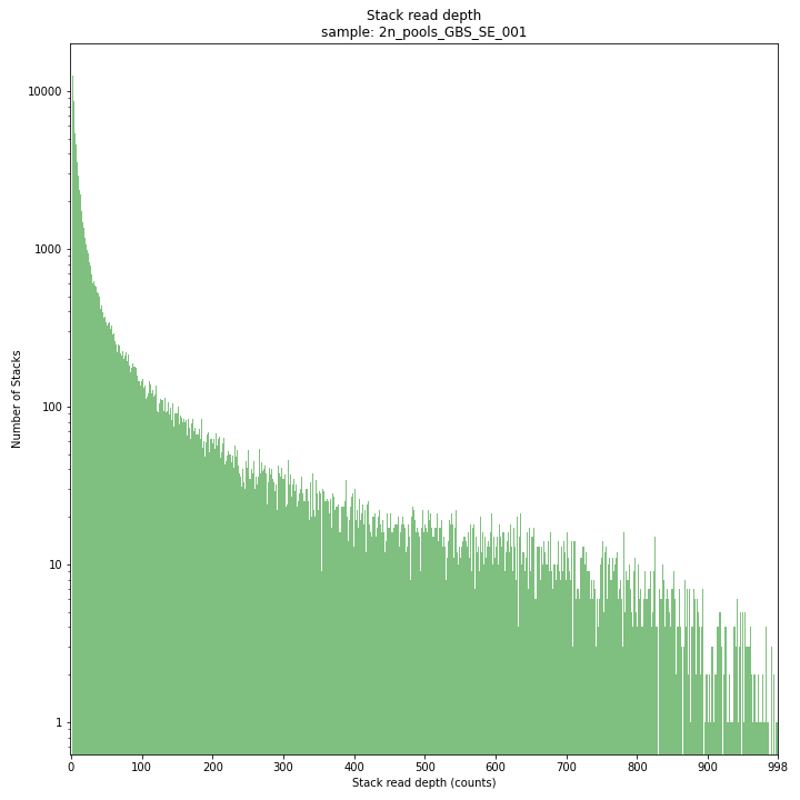
The Stack read depth distribution typically follows a left-skewed distribution, with many loci with relatively low read depth, and few loci at comparably high read depth. The shape of the read depth distribution results from differences in PCR-amplification and sequencing efficiency between GBS-fragments due to variation in fragment length, GC-content, and other factors. Loci with relatively high read depth are typically derived from repeat sequences that are mapped onto a single representative locus in the reference sequence.

_________________________________________________________________________________________________

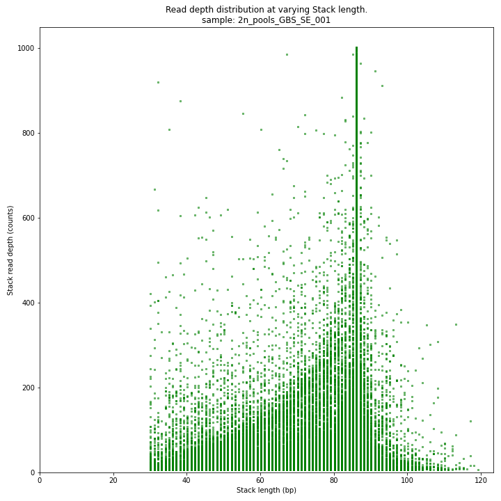
The Stack read depth and read length correlation distribution is expected to follow the Stack length distribution. It is recommended to not fill in the --max_stack_depth and --max_cluster_depth options (defaulting to infinite) during a trial run and to subsequently choose these values based on this (and the StackCluster.LengthDepthCorrelation scatter) plot. Extremely deeply sequenced loci are often short sequence repeats originitating from different loci on the genome but mapping on a single one.

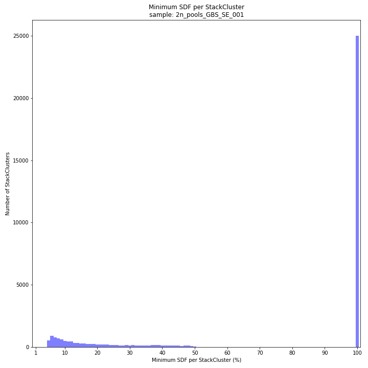
SMAP delineate run with --plot all plots the StackCluster mapping characteristics such as: the length, the read depth, the number of overlapping Stacks, and the Fraction of Stack read depth/total StackCluster read Depth (SDF).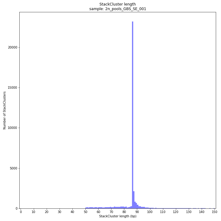

The majority of loci is expected to show StackCluster length similar to maximal read length (in this case 86 bp, after barcode and RE trimming of a 100 bp read). StackCluster length is defined by the outermost SMAPs after overlap of the underlying Stacks. Short Stacks can thus ‘hide’ under longer StackClusters, or two partially overlapping Stacks can increase total StackCluster length, slightly increasing the StackCluster length distribution compared to the Stack length distribution.

_________________________________________________________________________________________________

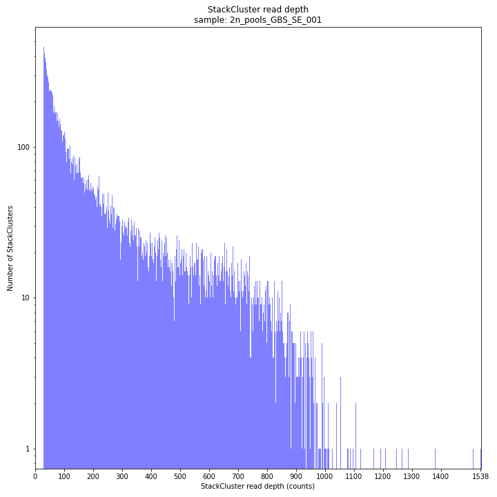
The StackCluster read depth distribution typically follows a left-skewed distribution, just like the Stack read depth distribution. Read depth values are slightly higher as StackClusters contain the sum of the underlying Stack read depths.

_________________________________________________________________________________________________

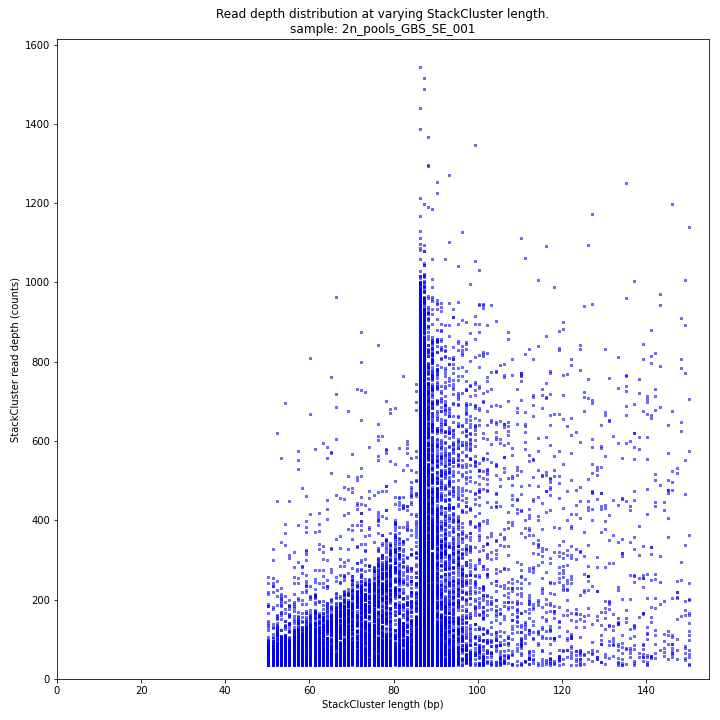
The StackCluster read depth and length correlation distribution is expected to follow the StackCluster length distribution. It is recommended to not fill in the --max_stack_depth and --max_cluster_depth options (defaulting to infinite) during a trial run and to subsequently choose these values based on this (and the Stack.LengthDepthCorrelation scatter) plot. Extremely deeply sequenced loci are often short sequence repeats originitating from different loci on the genome but mapping on a single one.

_________________________________________________________________________________________________

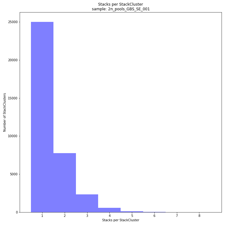
The distribution of the number of Stacks per StackCluster across all loci per sample indicates the abundance of read mapping polymorphisms in the GBS data. By definition, in diploid individuals, a StackCluster can contain 1 or 2 Stacks which are then delineated by 2 or 3 and 4 SMAPs, respectively (see scheme below). Therefore in diploid pools, the theoretical number of Stacks possible in a StackCluster is equal to 2 * the number of individuals in the pool. StackClusters with excess numbers of Stacks can be removed using the option -l or --max_stack_number. For diploid individuals, the recommended value for this option is 2, for pools it depends on the number of individuals in the pool and the genetic differentiation between these individuals.

_________________________________________________________________________________________________

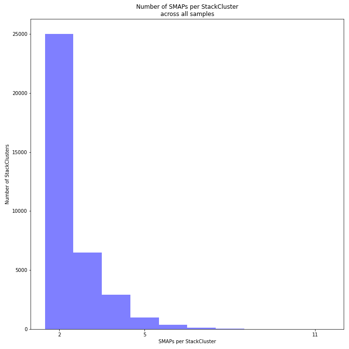
The image above depicts the number of SMAPs per StackCluster. By definition, 2 SMAPs result in either a single Stack or 2 Stacks without length polymorphisms but with SNPs. In diploids, the maximum number of SMAPs per StackCluster is 4; 2 Stacks with different start and stop positions. This situation is rare and the majority of StackClusters are expected to contain 2 or 3 SMAPs. Therefore in pools the absolute maximum number of SMAPs in a StackCluster is 4* the number of samples in a pool, but the majority of StackClusters are expected to have 2* to 3* the number of samples in a pool. StackClusters with excess Stacks (incorporation of SMAPs and SNPs) can be removed using the option -l or --max_stack_number.

_________________________________________________________________________________________________

text

SMAP delineate by default plots the MergedCluster mapping characteristics such as: Length, read depth, number of overlapping Stacks, number of Samples that contribute to a MergedCluster (Completeness).

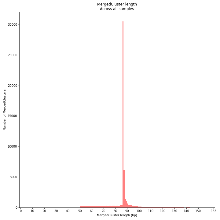
MergedCluster length is defined by the outermost SMAPs after overlap of all StackClusters per locus across all samples. The MergedCluster length distribution is expected to be similar or slightly longer compared to the StackCluster length distribution, but a clear single peak is expected at the maximum read length. High between-sample genetic variation in the sample set is expected to increase MergedCluster length compared to StackCluster length.

_________________________________________________________________________________________________

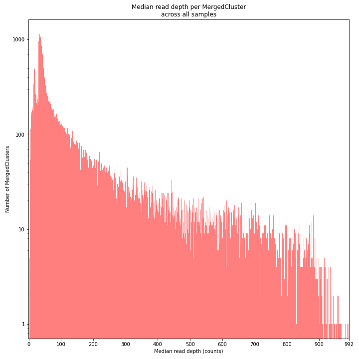
The median MergedCluster read depth distribution is a combination of the different StackCluster distributions. It gives an idea of how many loci are shared between at least half of the samples at at least a given read depth. The more similar this distribution is to each individual StackCluster read depth plot, the more complete the data are.

_________________________________________________________________________________________________

The distribution of the number of SMAPs per locus shows the abundance of read mapping polymorphisms across the sample set. This distribution is key to evaluating if it is crucial in your sample set to take read mapping polymorphisms into account. The majority of MergedClusters usually contain 2 SMAPs; in these loci, all reads per locus in the sample set have the same read mapping start and end positions. Loci with increasing numbers of SMAPs across the sample set are usually less abundant. The frequency of InDels and SNPs (causing alternative SMAPs) across the sample set is expected to be proportional to the genetic diversity displayed in read mapping polymorphisms (i.e. numbers of SMAPs per MergedCluster, see scheme below). Please note that technical artefacts, such as incorrect read trimming, also contribute to alternative read mapping polymorphisms across the sample set, and should be eliminated to avoid mistaking that as biological genetic diversity. See the section Recommendations and Troubleshooting for more details.

_________________________________________________________________________________________________

The distribution of completeness scores per MergedCluster across the sample set shows the fraction of the loci that have sufficient read depth in only a few samples (left side, lower completeness), and the fraction of loci that is commonly detected across the sample set (right side, higher completeness). This distribution is key to predicting missingness in the genotype calling table (sample-genotype matrix) for the sample set after downstream analysis. Each sample may have a similar total number of GBS loci (see read depth vs StackCluster saturation curve), but a small fraction may be shared across samples. The higher the genetic diversity across the sample set, the higher the number of sample-specific unique alleles and loci, the more left-skew in the completeness distribution, the lower the number of shared loci, and the more the total number of loci across the entire sample set is inflated.

The saturation curve shows if the total number of reads obtained per sample leads to the maximum number of detected StacksClusters per sample. Each circle in the graph is a single sample.

SMAP delineate run with --plot all plots the abundance of special features in the reference-read alignment (scored as Cigar strings). This graph shows the number of reads that include at least one occurence of H (hard clipping), S (soft clipping), D (deletion) or I (insertion), compared to the total number of reads in the BAM file. This abundance profile is a predictor for the number of expected read mapping polymorphisms, and should be in line with the distribution of the number of Stacks and SMAPs per StackCluster (per sample), and the number of SMAPs per MergedCluster (across the sample set).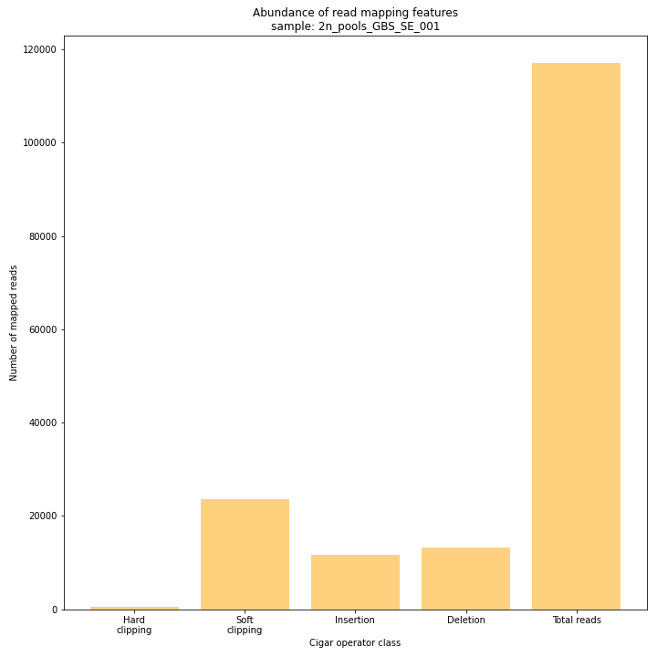

Tab command shows a typical command to run SMAP delineate for double-enzyme GBS, merged reads in pools.

Tabs for subsequent steps of Stack delineation show typical graphical results together with explanation about step-specific parameters.

smap delineate /path/to/BAM/ -mapping_orientation ignore -p 8 --plot all --plot_type png --name 2n_pools_GBS-PE -f 50 -g 300 --min_stack_depth 3 --max_stack_depth 2000 --min_cluster_depth 30 --max_cluster_depth 3000 --max_stack_number 10 --min_stack_depth_fraction 5 --completeness 1 --max_smap_number 20
SMAP delineate run with --plot all plots the distribution of the length and read depth per Stack. Stacks are defined by start and end positions on the reference sequence, hence stacks can be shorter or longer than the longest read length.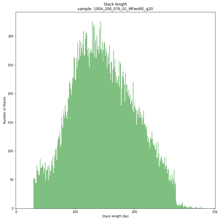

These merged reads were constructed from 136 bp each paired-end reads. Therefore with a minimum merging overlap of 10, the maximum merged read length becomes 262 bp. Any Stack longer than this length contains deletions which alters the mapping start and end positions on the reference sequence. Of course a minimum overlap of 10 does not exclude larger overlaps, therefore it is possible to merge two short reads (e.g. 40 bp) with a complete overlap and obtain a 40 bp Stack. Moreover, there is a PCR and sequencing bias towards these short reads as they are amplified faster.

_________________________________________________________________________________________________

The Stack read depth distribution typically follows a left-skewed distribution, with many loci with relatively low read depth, and few loci at comparably high read depth. The shape of the read depth distribution results from differences in PCR-amplification and sequencing efficiency between GBS-fragments due to variation in fragment length, GC-content, and other factors. Loci with relatively high read depth are typically derived from repeat sequences that are mapped onto a single representative locus in the reference sequence.

_________________________________________________________________________________________________

The Stack read depth and read length correlation distribution is expected to follow the Stack length distribution. It is recommended to not fill in the --max_stack_depth and --max_cluster_depth options (defaulting to infinite) during a trial run and to subsequently choose these values based on this (and the StackCluster.LengthDepthCorrelation scatter) plot. Extremely deeply sequenced loci are often short sequence repeats originitating from different loci on the genome but mapping on a single one.

SMAP delineate run with --plot all plots the StackCluster mapping characteristics such as: the length, the read depth, the number of overlapping Stacks, and the Fraction of Stack read depth/total StackCluster read Depth (SDF).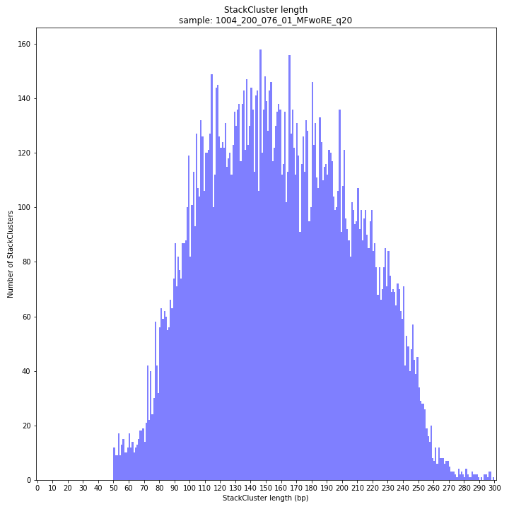

The majority of loci are expected to show a StackCluster length distribution (region covered by the Stacks) similar to the Stack length distribution, but shifted somewhat to the right. StackCluster length is defined by the outermost SMAPs after overlap of the underlying Stacks. Short Stacks can thus ‘hide’ under longer StackClusters, or two partially overlapping Stacks can increase total StackCluster length, slightly increasing the StackCluster length distribution compared to the Stack length distribution.

_________________________________________________________________________________________________

The StackCluster read depth distribution typically follows a left-skewed distribution, just like the Stack read depth distribution. Read depth values are slightly higher as StackClusters contain the sum of the underlying Stack read depths.

_________________________________________________________________________________________________

The StackCluster read depth and length correlation distribution is expected to follow the StackCluster length distribution. It is recommended to not fill in the --max_stack_depth and --max_cluster_depth options (defaulting to infinite) during a trial run and to subsequently choose these values based on this (and the Stack.LengthDepthCorrelation scatter) plot. Extremely deeply sequenced loci are often short sequence repeats originitating from different loci on the genome but mapping on a single one.

_________________________________________________________________________________________________

The distribution of the number of Stacks per StackCluster across all loci per sample indicates the abundance of read mapping polymorphisms in the GBS data. By definition, in diploid individuals, a StackCluster can contain 1 or 2 Stacks which are then delineated by 2 or 3 and 4 SMAPs, respectively (see scheme below). Therefore in diploid pools, the theoretical number of Stacks possible in a StackCluster is equal to 2 * the number of individuals in the pool. StackClusters with excess numbers of Stacks can be removed using the option -l or --max_stack_number. For diploid individuals, the recommended value for this option is 2, for pools it depends on the number of individuals in the pool and the genetic differentiation between these individuals.

_________________________________________________________________________________________________

The image above depicts the number of SMAPs per StackCluster. By definition, 2 SMAPs result in either a single Stack or 2 Stacks without length polymorphisms but with SNPs. In diploids, the maximum number of SMAPs per StackCluster is 4; 2 Stacks with different start and stop positions. This situation is rare and the majority of StackClusters are expected to contain 2 or 3 SMAPs. Therefore in pools the absolute maximum number of SMAPs in a StackCluster is 4* the number of samples in a pool, but the majority of StackClusters are expected to have 2* to 3* the number of samples in a pool. StackClusters with excess Stacks (incorporation of SMAPs and SNPs) can be removed using the option -l or --max_stack_number.

_________________________________________________________________________________________________

text

SMAP delineate by default plots the MergedCluster mapping characteristics such as: Length, read depth, number of overlapping Stacks, number of Samples that contribute to a MergedCluster (Completeness).

MergedCluster length is defined by the outermost SMAPs after overlap of all StackClusters per locus across all samples. The MergedCluster length distribution is expected to be similar or slightly longer compared to the StackCluster length distribution, but a clear single peak is expected at the maximum read length. High between-sample genetic variation in the sample set is expected to increase MergedCluster length compared to StackCluster length.

_________________________________________________________________________________________________

The median MergedCluster read depth distribution is a combination of the different StackCluster distributions. It gives an idea of how many loci are shared between at least half of the samples at at least a given read depth. The more similar this distribution is to each individual StackCluster read depth plot, the more complete the data are.

_________________________________________________________________________________________________

The distribution of the number of SMAPs per locus shows the abundance of read mapping polymorphisms across the sample set. This distribution is key to evaluating if it is crucial in your sample set to take read mapping polymorphisms into account. The majority of MergedClusters usually contain 2 SMAPs; in these loci, all reads per locus in the sample set have the same read mapping start and end positions. Loci with increasing numbers of SMAPs across the sample set are usually less abundant. The frequency of InDels and SNPs (causing alternative SMAPs) across the sample set is expected to be proportional to the genetic diversity displayed in read mapping polymorphisms (i.e. numbers of SMAPs per MergedCluster, see scheme below). Please note that technical artefacts, such as incorrect read trimming, also contribute to alternative read mapping polymorphisms across the sample set, and should be eliminated to avoid mistaking that as biological genetic diversity. See the section Recommendations and Troubleshooting for more details.

_________________________________________________________________________________________________

The distribution of completeness scores per MergedCluster across the sample set shows the fraction of the loci that have sufficient read depth in only a few samples (left side, lower completeness), and the fraction of loci that is commonly detected across the sample set (right side, higher completeness). This distribution is key to predicting missingness in the genotype calling table (sample-genotype matrix) for the sample set after downstream analysis. Each sample may have a similar total number of GBS loci (see read depth vs StackCluster saturation curve), but a small fraction may be shared across samples. The higher the genetic diversity across the sample set, the higher the number of sample-specific unique alleles and loci, the more left-skew in the completeness distribution, the lower the number of shared loci, and the more the total number of loci across the entire sample set is inflated.

The saturation curve shows if the total number of reads obtained per sample leads to the maximum number of detected StacksClusters per sample. Each circle in the graph is a single sample.

SMAP delineate run with --plot all plots the abundance of special features in the reference-read alignment (scored as Cigar strings). This graph shows the number of reads that include at least one occurence of H (hard clipping), S (soft clipping), D (deletion) or I (insertion), compared to the total number of reads in the BAM file. This abundance profile is a predictor for the number of expected read mapping polymorphisms, and should be in line with the distribution of the number of Stacks and SMAPs per StackCluster (per sample), and the number of SMAPs per MergedCluster (across the sample set).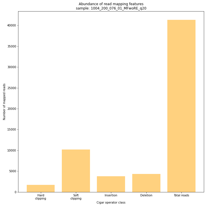

Tab command shows a typical command to run SMAP delineate for single-enzyme GBS, merged reads in tetraploid individuals.

Tabs for subsequent steps of Stack delineation show typical graphical results together with explanation about step-specific parameters.

smap delineate /path/to/BAM/ -mapping_orientation ignore -p 8 --plot all --plot_type png --name 4n_ind_GBS-PE -f 50 -g 300 --min_stack_depth 2 --max_stack_depth 1500 --min_cluster_depth 10 --max_cluster_depth 3000 --max_stack_number 4 --min_stack_depth_fraction 10 --completeness 1 --max_smap_number 20
SMAP delineate run with --plot all plots the distribution of the length and read depth per Stack. Stacks are defined by start and end positions on the reference sequence, hence stacks can be shorter or longer than the longest read length.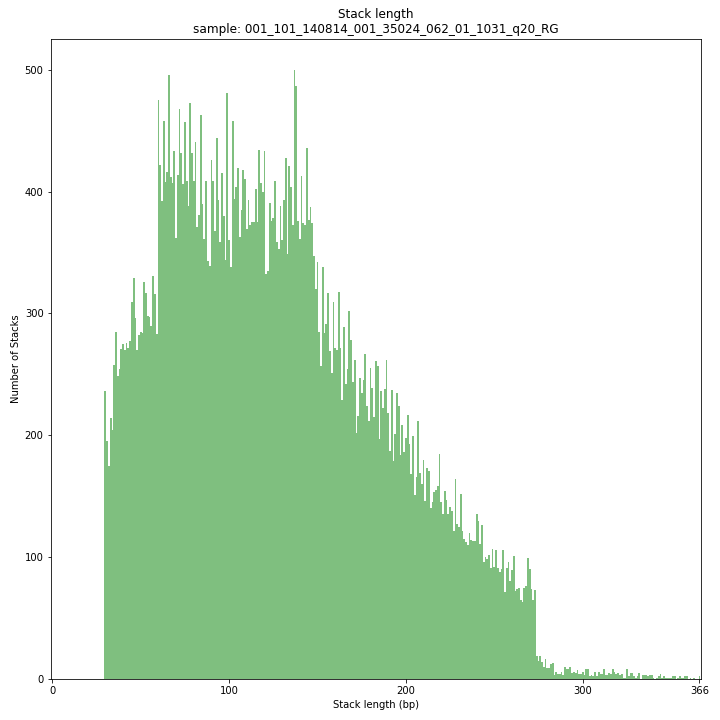

These merged reads were constructed from 136 bp each paired-end reads. Therefore with a minimum merging overlap of 10, the maximum merged read length becomes 262 bp. Any Stack longer than this contains deletions which alter the start and end positions on the reference sequence. Of course a minimum overlap of 10 does not exclude larger overlaps, therefore it is possible to merge two short reads (e.g. 40 bp) with a complete overlap and obtain a 40 bp Stack. Moreover, there is a PCR and sequencing bias towards these short reads as they are amplified faster.

_________________________________________________________________________________________________

The Stack read depth distribution typically follows a left-skewed distribution, with many loci with relatively low read depth, and few loci at comparably high read depth. The shape of the read depth distribution results from differences in PCR-amplification and sequencing efficiency between GBS-fragments due to variation in fragment length, GC-content, and other factors. Loci with relatively high read depth are typically derived from repeat sequences that are mapped onto a single representative locus in the reference sequence.

_________________________________________________________________________________________________

The Stack read depth and read length correlation distribution is expected to follow the Stack length distribution. It is recommended to not fill in the --max_stack_depth and --max_cluster_depth options (defaulting to infinite) during a trial run and to subsequently choose these values based on this (and the StackCluster.LengthDepthCorrelation scatter) plot. Extremely deeply sequenced loci are often short sequence repeats originitating from different loci on the genome but mapping on a single one.

SMAP delineate run with --plot all plots the StackCluster mapping characteristics such as: the length, the read depth, the number of overlapping Stacks, and the Fraction of Stack read depth/total StackCluster read Depth (SDF).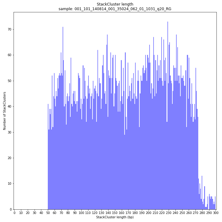

The majority of loci are expected to show a StackCluster length distribution similar to the Stack length distribution, but shifted somewhat to the right. StackCluster length is defined by the outermost SMAPs after overlap of the underlying Stacks. Short Stacks can thus ‘hide’ under longer StackClusters, or two partially overlapping Stacks can increase total StackCluster length, slightly increasing the StackCluster length distribution compared to the Stack length distribution.

_________________________________________________________________________________________________

The StackCluster read depth distribution typically follows a left-skewed distribution, just like the Stack read depth distribution. Read depth values are slightly higher as StackClusters contain the sum of the underlying Stack read depths.

_________________________________________________________________________________________________

The StackCluster read depth and length correlation distribution is expected to follow the StackCluster length distribution. It is recommended to not fill in the --max_stack_depth and --max_cluster_depth options (defaulting to infinite) during a trial run and to subsequently choose these values based on this (and the Stack.LengthDepthCorrelation scatter) plot. Extremely deeply sequenced loci are often short sequence repeats originitating from different loci on the genome but mapping on a single one.

_________________________________________________________________________________________________

The distribution of the number of Stacks per StackCluster across all loci per sample indicates the abundance of read mapping polymorphisms in the GBS data. By definition, in tetraploids, a StackCluster can contain 1 up to 4 Stacks which are then delineated by 2 up to 8 SMAPs, respectively (see scheme below). StackClusters with excess numbers of Stacks can be removed using the option -l or --max_stack_number. For tetraploid individuals, the recommended value for this option is 4.

_________________________________________________________________________________________________

The image above depicts the number of SMAPs per StackCluster. By definition, 2 SMAPs result in either a single Stack or 2 Stacks without length polymorphisms but with SNPs. In tetraploids, the maximum number of SMAPs per StackCluster is 8; 4 Stacks with different start and stop positions. This situation is rare and the majority of StackClusters are expected to contain 2 to 4 SMAPs. StackClusters with excess Stacks (incorporation of SMAPs and SNPs) can be removed using the option -l or --max_stack_number, for tetraploids the recommended value for this option is 8.

_________________________________________________________________________________________________

text

SMAP delineate by default plots the MergedCluster mapping characteristics such as: Length, read depth, number of overlapping Stacks, number of Samples that contribute to a MergedCluster (Completeness).

MergedCluster length is defined by the outermost SMAPs after overlap of all StackClusters per locus across all samples. The MergedCluster length distribution is expected to be similar or slightly longer compared to the StackCluster length distribution, but a clear single peak is expected at the maximum read length. High between-sample genetic variation in the sample set is expected to increase MergedCluster length compared to StackCluster length.

_________________________________________________________________________________________________

The median MergedCluster read depth distribution is a combination of the different StackCluster distributions. It gives an idea of how many loci are shared between at least half of the samples at at least a given read depth. The more similar this distribution is to each individual StackCluster read depth plot, the more complete the data are.

_________________________________________________________________________________________________

The distribution of the number of SMAPs per locus shows the abundance of read mapping polymorphisms across the sample set. This distribution is key to evaluating if it is crucial in your sample set to take read mapping polymorphisms into account. The majority of MergedClusters usually contain 2 SMAPs; in these loci, all reads per locus in the sample set have the same read mapping start and end positions. Loci with increasing numbers of SMAPs across the sample set are usually less abundant. The frequency of InDels and SNPs (causing alternative SMAPs) across the sample set is expected to be proportional to the genetic diversity displayed in read mapping polymorphisms (i.e. numbers of SMAPs per MergedCluster, see scheme below). Please note that technical artefacts, such as incorrect read trimming, also contribute to alternative read mapping polymorphisms across the sample set, and should be eliminated to avoid mistaking that as biological genetic diversity. See the section Recommendations and Troubleshooting for more details.

_________________________________________________________________________________________________

The distribution of completeness scores per MergedCluster across the sample set shows the fraction of the loci that have sufficient read depth in only a few samples (left side, lower completeness), and the fraction of loci that is commonly detected across the sample set (right side, higher completeness). This distribution is key to predicting missingness in the genotype calling table (sample-genotype matrix) for the sample set after downstream analysis. Each sample may have a similar total number of GBS loci (see read depth vs StackCluster saturation curve), but a small fraction may be shared across samples. The higher the genetic diversity across the sample set, the higher the number of sample-specific unique alleles and loci, the more left-skew in the completeness distribution, the lower the number of shared loci, and the more the total number of loci across the entire sample set is inflated.

The saturation curve shows if the total number of reads obtained per sample leads to the maximum number of detected StacksClusters per sample. Each circle in the graph is a single sample.

SMAP delineate run with --plot all plots the abundance of special features in the reference-read alignment (scored as Cigar strings). This graph shows the number of reads that include at least one occurence of H (hard clipping), S (soft clipping), D (deletion) or I (insertion), compared to the total number of reads in the BAM file. This abundance profile is a predictor for the number of expected read mapping polymorphisms, and should be in line with the distribution of the number of Stacks and SMAPs per StackCluster (per sample), and the number of SMAPs per MergedCluster (across the sample set).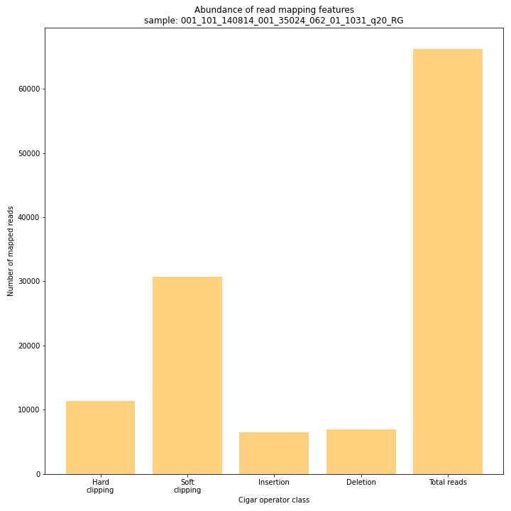

Tab command shows a typical command to run SMAP delineate for single-enzyme GBS, merged reads in pools.

Tabs for subsequent steps of Stack delineation show typical graphical results together with explanation about step-specific parameters.

smap delineate /path/to/BAM/ -mapping_orientation ignore -p 8 --plot all --plot_type png --name 4n_pools_GBS-PE -f 50 -g 300 --min_stack_depth 3 --max_stack_depth 1000 --min_cluster_depth 30 --max_cluster_depth 1500 --max_stack_number 20 --min_stack_depth_fraction 5 --completeness 1 --max_smap_number 20
SMAP delineate run with --plot all plots the distribution of the length and read depth per Stack. Stacks are defined by start and end positions on the reference sequence, hence stacks can be shorter or longer than the longest read length.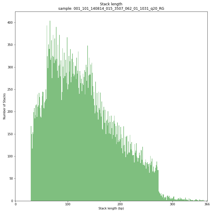

These merged reads were constructed from 136 bp each paired-end reads. Therefore with a minimum merging overlap of 10, the maximum merged read length becomes 262 bp. Any Stack longer than this contains deletions which alter the start and end positions on the reference sequence. Of course a minimum overlap of 10 does not exclude larger overlaps, therefore it is possible to merge two short reads (e.g. 40 bp) with a complete overlap and obtain a 40 bp Stack. Moreover, there is a PCR and sequencing bias towards these short reads as they are amplified faster.

_________________________________________________________________________________________________

The Stack read depth distribution typically follows a left-skewed distribution, with many loci with relatively low read depth, and few loci at comparably high read depth. The shape of the read depth distribution results from differences in PCR-amplification and sequencing efficiency between GBS-fragments due to variation in fragment length, GC-content, and other factors. Loci with relatively high read depth are typically derived from repeat sequences that are mapped onto a single representative locus in the reference sequence.

_________________________________________________________________________________________________

The Stack read depth and read length correlation distribution is expected to follow the Stack length distribution. It is recommended to not fill in the --max_stack_depth and --max_cluster_depth options (defaulting to infinite) during a trial run and to subsequently choose these values based on this (and the StackCluster.LengthDepthCorrelation scatter) plot. Extremely deeply sequenced loci are often short sequence repeats originitating from different loci on the genome but mapping on a single one.

SMAP delineate run with --plot all plots the StackCluster mapping characteristics such as: the length, the read depth, the number of overlapping Stacks, and the Fraction of Stack read depth/total StackCluster read Depth (SDF).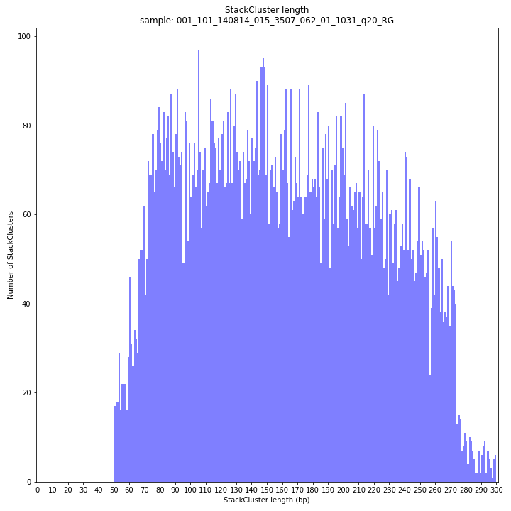

The majority of loci are expected to show a StackCluster length distribution (region covered by the Stacks) similar to the Stack length distribution, but shifted somewhat to the right. StackCluster length is defined by the outermost SMAPs after overlap of the underlying Stacks. Short Stacks can thus ‘hide’ under longer StackClusters, or two partially overlapping Stacks can increase total StackCluster length, slightly increasing the StackCluster length distribution compared to the Stack length distribution.

_________________________________________________________________________________________________

The StackCluster read depth distribution typically follows a left-skewed distribution, just like the Stack read depth distribution. Read depth values are slightly higher as StackClusters contain the sum of the underlying Stack read depths.

_________________________________________________________________________________________________

The StackCluster read depth and length correlation distribution is expected to follow the StackCluster length distribution. It is recommended to not fill in the --max_stack_depth and --max_cluster_depth options (defaulting to infinite) during a trial run and to subsequently choose these values based on this (and the Stack.LengthDepthCorrelation scatter) plot. Extremely deeply sequenced loci are often short sequence repeats originitating from different loci on the genome but mapping on a single one.

_________________________________________________________________________________________________

The distribution of the number of Stacks per StackCluster across all loci per sample indicates the abundance of read mapping polymorphisms in the GBS data. By definition, in diploid individuals, a StackCluster can contain 1 up to 4 Stacks which are then delineated by 2 up to 8 SMAPs, respectively (see scheme below). Therefore in tetraploid pools, the theoretical number of Stacks possible in a StackCluster is equal to 4 * the number of individuals in the pool. StackClusters with excess numbers of Stacks can be removed using the option -l or --max_stack_number. For tetraploid individuals, the recommended value for this option is 4, for pools it depends on the number of individuals in the pool and the genetic differentiation between these individuals.

_________________________________________________________________________________________________

The image above depicts the number of SMAPs per StackCluster. By definition, 2 SMAPs result in either a single Stack or 2 Stacks without length polymorphisms but with SNPs. In tetraploids, the maximum number of SMAPs per StackCluster is 8; 4 Stacks with different start and stop positions. This situation is rare and the majority of StackClusters are expected to contain 2 to 4 SMAPs. Therefore in pools the absolute maximum number of SMAPs in a StackCluster is 8* the number of samples in a pool, but the majority of StackClusters are expected to have 2* to 4* the number of samples in a pool. StackClusters with excess Stacks (incorporation of SMAPs and SNPs) can be removed using the option -l or --max_stack_number.

_________________________________________________________________________________________________

text

SMAP delineate by default plots the MergedCluster mapping characteristics such as: Length, read depth, number of overlapping Stacks, number of Samples that contribute to a MergedCluster (Completeness).

MergedCluster length is defined by the outermost SMAPs after overlap of all StackClusters per locus across all samples. The MergedCluster length distribution is expected to be similar or slightly longer compared to the StackCluster length distribution, but a clear single peak is expected at the maximum read length. High between-sample genetic variation in the sample set is expected to increase MergedCluster length compared to StackCluster length.

_________________________________________________________________________________________________

The median MergedCluster read depth distribution is a combination of the different StackCluster distributions. It gives an idea of how many loci are shared between at least half of the samples at at least a given read depth. The more similar this distribution is to each individual StackCluster read depth plot, the more complete the data are.

_________________________________________________________________________________________________

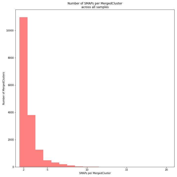
The distribution of the number of SMAPs per locus shows the abundance of read mapping polymorphisms across the sample set. This distribution is key to evaluating if it is crucial in your sample set to take read mapping polymorphisms into account. The majority of MergedClusters usually contain 2 SMAPs; in these loci, all reads per locus in the sample set have the same read mapping start and end positions. Loci with increasing numbers of SMAPs across the sample set are usually less abundant. The frequency of InDels and SNPs (causing alternative SMAPs) across the sample set is expected to be proportional to the genetic diversity displayed in read mapping polymorphisms (i.e. numbers of SMAPs per MergedCluster, see scheme below). Please note that technical artefacts, such as incorrect read trimming, also contribute to alternative read mapping polymorphisms across the sample set, and should be eliminated to avoid mistaking that as biological genetic diversity. See the section Recommendations and Troubleshooting for more details.

_________________________________________________________________________________________________

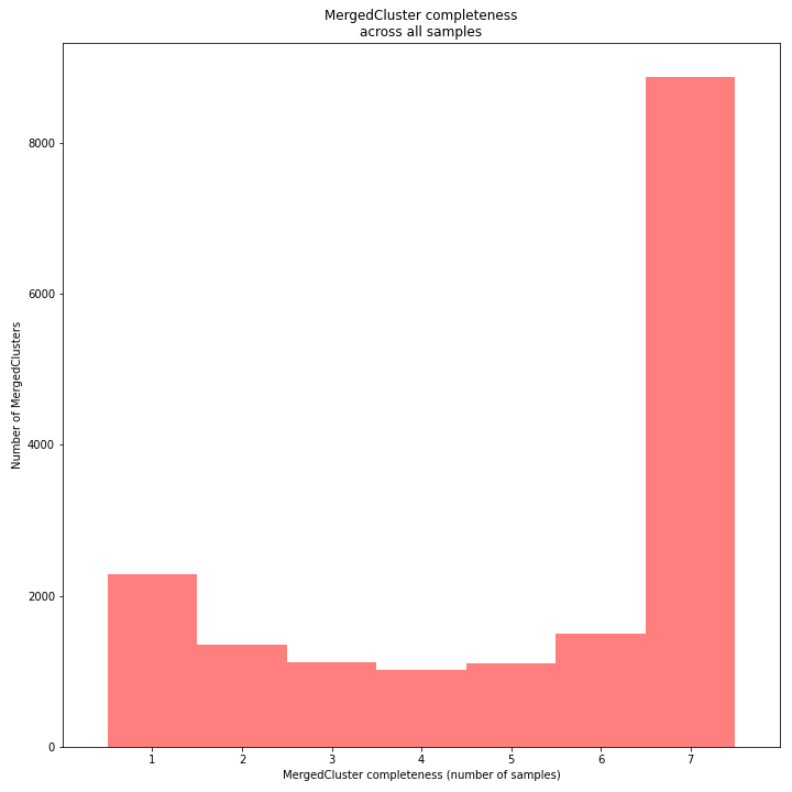
The distribution of completeness scores per MergedCluster across the sample set shows the fraction of the loci that have sufficient read depth in only a few samples (left side, lower completeness), and the fraction of loci that is commonly detected across the sample set (right side, higher completeness). This distribution is key to predicting missingness in the genotype calling table (sample-genotype matrix) for the sample set after downstream analysis. Each sample may have a similar total number of GBS loci (see read depth vs StackCluster saturation curve), but a small fraction may be shared across samples. The higher the genetic diversity across the sample set, the higher the number of sample-specific unique alleles and loci, the more left-skew in the completeness distribution, the lower the number of shared loci, and the more the total number of loci across the entire sample set is inflated.

The saturation curve shows if the total number of reads obtained per sample leads to the maximum number of detected StacksClusters per sample. Each circle in the graph is a single sample.

SMAP delineate run with --plot all plots the abundance of special features in the reference-read alignment (scored as Cigar strings). This graph shows the number of reads that include at least one occurence of H (hard clipping), S (soft clipping), D (deletion) or I (insertion), compared to the total number of reads in the BAM file. This abundance profile is a predictor for the number of expected read mapping polymorphisms, and should be in line with the distribution of the number of Stacks and SMAPs per StackCluster (per sample), and the number of SMAPs per MergedCluster (across the sample set).