Scope & Usage
Scope
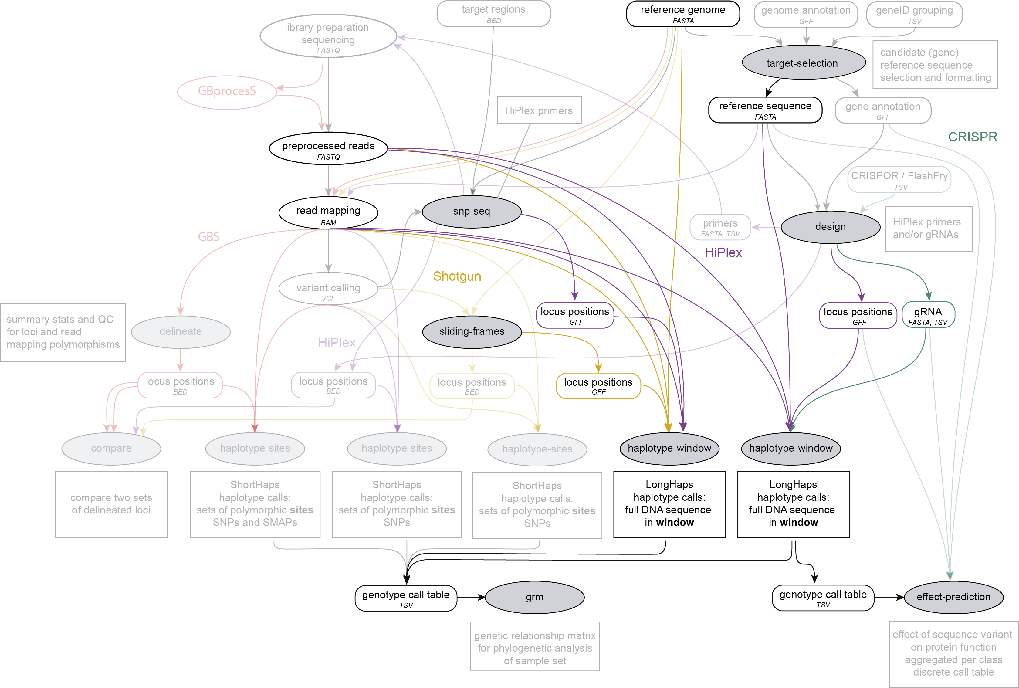
Integration in the SMAP workflow
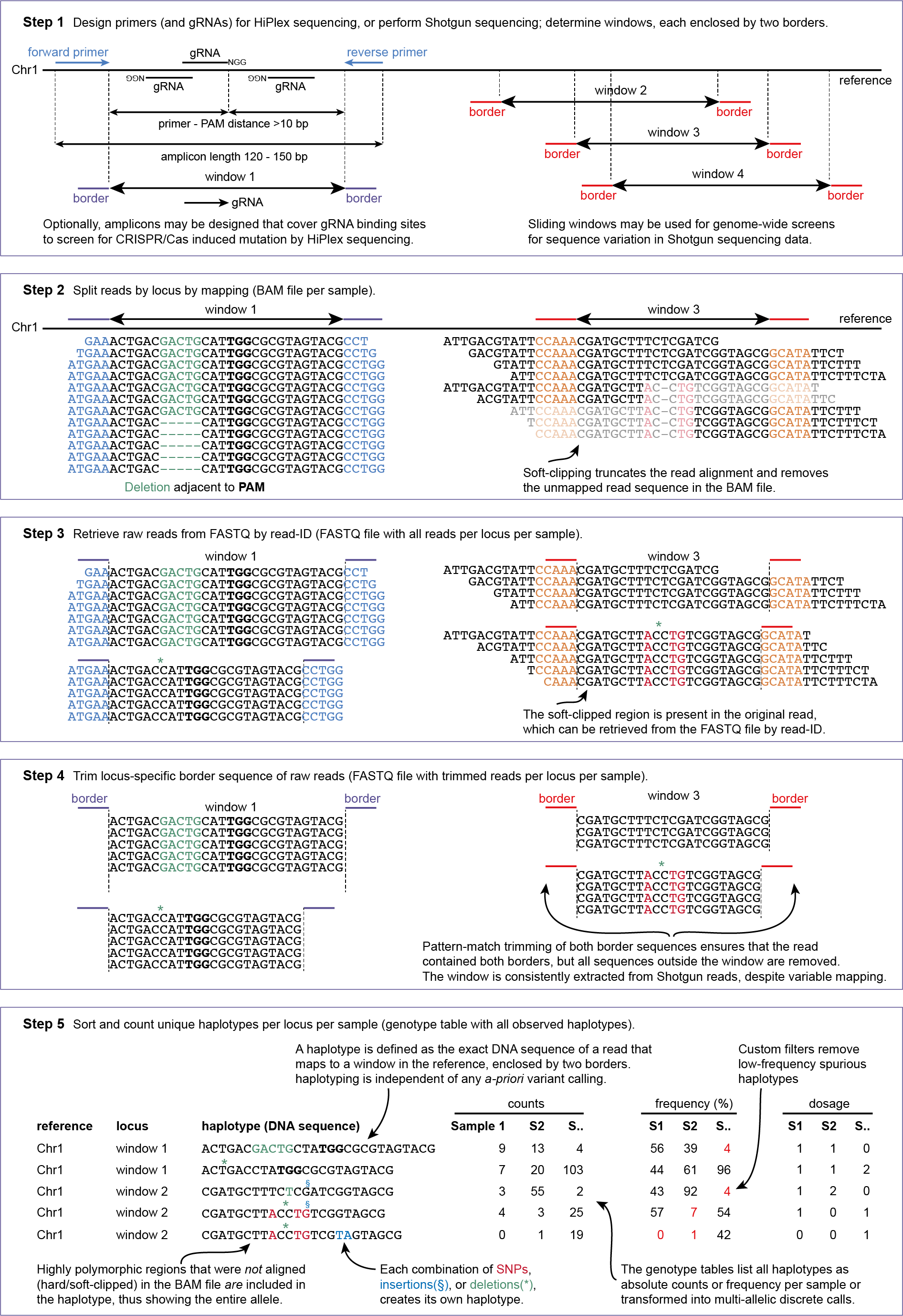
SMAP haplotype-window takes a reference sequence, a set of locus positions (windows defined by pairs of borders, created by SMAP snp-seq, SMAP design, or SMAP sliding-frames), a set of corresponding FASTQ and BAM files. Optionally, it can take a list of gRNA sequences created by SMAP design. Genotype call tables created by SMAP haplotype-window may further be analysed with SMAP relatedness, or with SMAP effect-prediction.
Required input
The FASTA file containing the reference sequence. Typically, whole genome reference sequences are used for Shotgun sequencing data, while a reference consisting of selected candidate genes may be created by SMAP target-selection for HiPlex data.
1. Name of the sequence in the reference that contains the Window.2. Source of the feature. [SMAP haplotype-window].3. Feature type. Because in SMAP haplotype-window pairs of borders define windows, two feature types are used: border_upstream and border_downstream. Each line in the GFF is one of those borders. Borders always come in pairs.4. The start coordinate of the border region [in the 1-based GFF coordinate system].5. The end coordinate of the border region [in the 1-based GFF coordinate system, value must always be higher than column 4].6. Score. Irrelevant for SMAP haplotype-window [.].7. Orientation of the border [always +].8. Phase. Irrelevant for SMAP haplotype-window [.].9. Attributes of the border, the field 'NAME=' is required. This field is used to pair borders (by exact 'NAME=' matching), and define the corresponding window regions. The field Name must be unique for each window and will be used to name loci in the haplotype frequency tables.
For HiPlex data it is advised to use the 8-10 nucleotides on the 3’ of the primer binding site, where they flank the window (to extract the sequence read region inbetween the primers).
ACD11
SMAP
CRISPR_border_up
124
133
.
+
.
NAME=ACD11_1
ACD11
SMAP
CRISPR_border_down
223
232
.
+
.
NAME=ACD11_1
ACD11
SMAP
CRISPR_border_up
864
873
.
+
.
NAME=ACD11_2
ACD11
SMAP
CRISPR_border_down
970
979
.
+
.
NAME=ACD11_2
ACD11
SMAP
CRISPR_border_up
4273
4282
.
+
.
NAME=ACD11_3
ACD11
SMAP
CRISPR_border_down
4393
4402
.
+
.
NAME=ACD11_3
AGD2
SMAP
CRISPR_border_up
726
735
.
+
.
NAME=AGD2_1
AGD2
SMAP
CRISPR_border_down
821
830
.
+
.
NAME=AGD2_1
AGD2
SMAP
CRISPR_border_up
4047
4056
.
+
.
NAME=AGD2_2
AGD2
SMAP
CRISPR_border_down
4154
4163
.
+
.
NAME=AGD2_2
Chr1
SMAP
CRISPR_border_up
1
10
.
+
.
NAME=Chr1_window_1
Chr1
SMAP
CRISPR_border_down
61
70
.
+
.
NAME=Chr1_window_1
Chr1
SMAP
CRISPR_border_up
21
30
.
+
.
NAME=Chr1_window_2
Chr1
SMAP
CRISPR_border_down
81
90
.
+
.
NAME=Chr1_window_2
Chr1
SMAP
CRISPR_border_up
41
50
.
+
.
NAME=Chr1_window_3
Chr1
SMAP
CRISPR_border_down
101
110
.
+
.
NAME=Chr1_window_3
Chr2
SMAP
CRISPR_border_up
61
70
.
+
.
NAME=Chr2_window_1
Chr2
SMAP
CRISPR_border_down
121
130
.
+
.
NAME=Chr2_window_1
Chr2
SMAP
CRISPR_border_up
81
90
.
+
.
NAME=Chr2_window_2
Chr2
SMAP
CRISPR_border_down
141
150
.
+
.
NAME=Chr2_window_2
A set of FASTQ files with preprocessed reads that need to be haplotyped. Any number of samples may be given and will be processed in parallel. All files per sample are matched by extension: .fq / .bam / .bam.bai. Therefore, the FASTQ files must have matching basenames compared to the BAM files: sample1.fq combined with sample1.bam and sample1.bam.bai. Optionally, FASTQ files may be gzipped: sample1.fq.gz.
A set of BAM files made with BWA-MEM using the respective reference sequence and FASTQ files.
Optional: a FASTA file containing the gRNA sequences, created by SMAP design, in case CRISPR was performed by stable transformation with a CRISPR/gRNA delivery vector, see also CRISPR.
Commands & options
The program has four mandatory positional arguments and multiple optional arguments.
Mandatory options for SMAP haplotype-window:
genome ################### (str) ### FASTA file with the reference genome sequence. The first positional mandatory argument after smap haplotype-window [no default].
borders ################## (str) ### GFF file with the coordinates of pairs of Borders that enclose a Window. Must contain NAME=<> in column 9 to denote the Window name. The second positional mandatory argument after smap haplotype-window [no default].
alignments_dir ############# (str) ### Path to the directory containing BAM and BAM index (BAI) files. All BAM files should be in the same directory. The third positional mandatory argument after smap haplotype-window. Should be indicated by absolute path or at least a “.” [default current directory].
sample_dir ################ (str) ### Path to the directory containing FASTQ files with the reads mapped to the reference genome to create the BAM files. The FASTQ file names must have the same prefix as the BAM files specified in alignments_dir. The fourth positional mandatory argument after smap haplotype-window [no default].
--write_sorted_sequences ############# Write FASTQ files containing the reads for each Window in a separate file per input sample [default off].-p, --processes ############ (int) ### Number of parallel processes [1].--memory_efficient ################# Reduces the memory load significantly, but increases time to calculate results.-o, --out ################ (str) ### Basename of the output file without extension [“”].-h, --help ###################### Show the full list of options. Disregards all other parameters.-v, --version #################### Show the version. Disregards all other parameters.--debug ######################### Enable verbose logging. Provides additional intermediate output files used for sample-specific QC.-–guides ################## (str) ### Optional FASTA file containing the sequences from gRNAs used in CRISPR/Cas genome editing. Useful when amplicons on the CRISPR/gRNA delivery vector are included in the HiPlex amplicon mixture. The most optimal name for the gRNA is Gene_amplicon_gRNA (e.g. AT1G01234_1_gRNA_001).-q, --min_mapping_quality #### (int) ### Minimum BAM mapping quality to retain reads for analysis [30].-c, --min_read_count ####### (int) ### Minimum total number of reads per locus per sample [0].-d, --max_read_count ####### (int) ### Maximum number of reads per locus per sample, read depth is calculated after filtering out the low frequency haplotypes (-f) [inf].-f, --min_haplotype_frequency # (int) ### Set minimum haplotype frequency (in %) to retain the haplotype in the genotyping table. Haplotypes above this threshold in at least one of the samples are retained. Haplotypes that never reach this threshold in any of the samples are removed [0].-j, --min_distinct_haplotypes # (int) ### Set minimum number of distinct haplotypes per locus across all samples. Loci that do not fit this criterium are removed from the final output [0].-k, --max_distinct_haplotypes # (int) ### Set maximum number of distinct haplotypes per locus across all samples. Loci that do not fit this criterium are removed from the final output [inf].--max_error ############# (float) ### The maximum error rate (between 0 and 1; but not exactly 1) for finding the border sequences in the reads. An error rate of 0 refers to exact match [0].-m, --mask_frequency ####### (float) ## Mask haplotype frequency values below this threshold for individual samples. Can be used to mask noise. Haplotype frequency values below -m are set to -u. Haplotypes are not removed removed from the genotype table based on this value, use --min_haplotype_frequency for this purpose instead.-u, --undefined_representation # (str) ### Value to use for non-existing or masked data [NaN].--cervus ########### Create genotype table in the format that can be used as input for Cervus parental analysis [default off].--plot ### (all, summary, nothing) ## Select which plots are generated. Choosing “nothing” disables plot generation. Passing “summary” only generates graphs with information for all samples, while “all” will also generate per-sample plots [default “summary”].-t, --plot_type ##### (png, pdf) ## Choose the file type for the plots [png].This option is primarily supported for diploids and tetraploids. Users can define their own custom frequency bounds for species with a higher ploidy, but this requires optimization based on the observed haplotype frequency distributions.
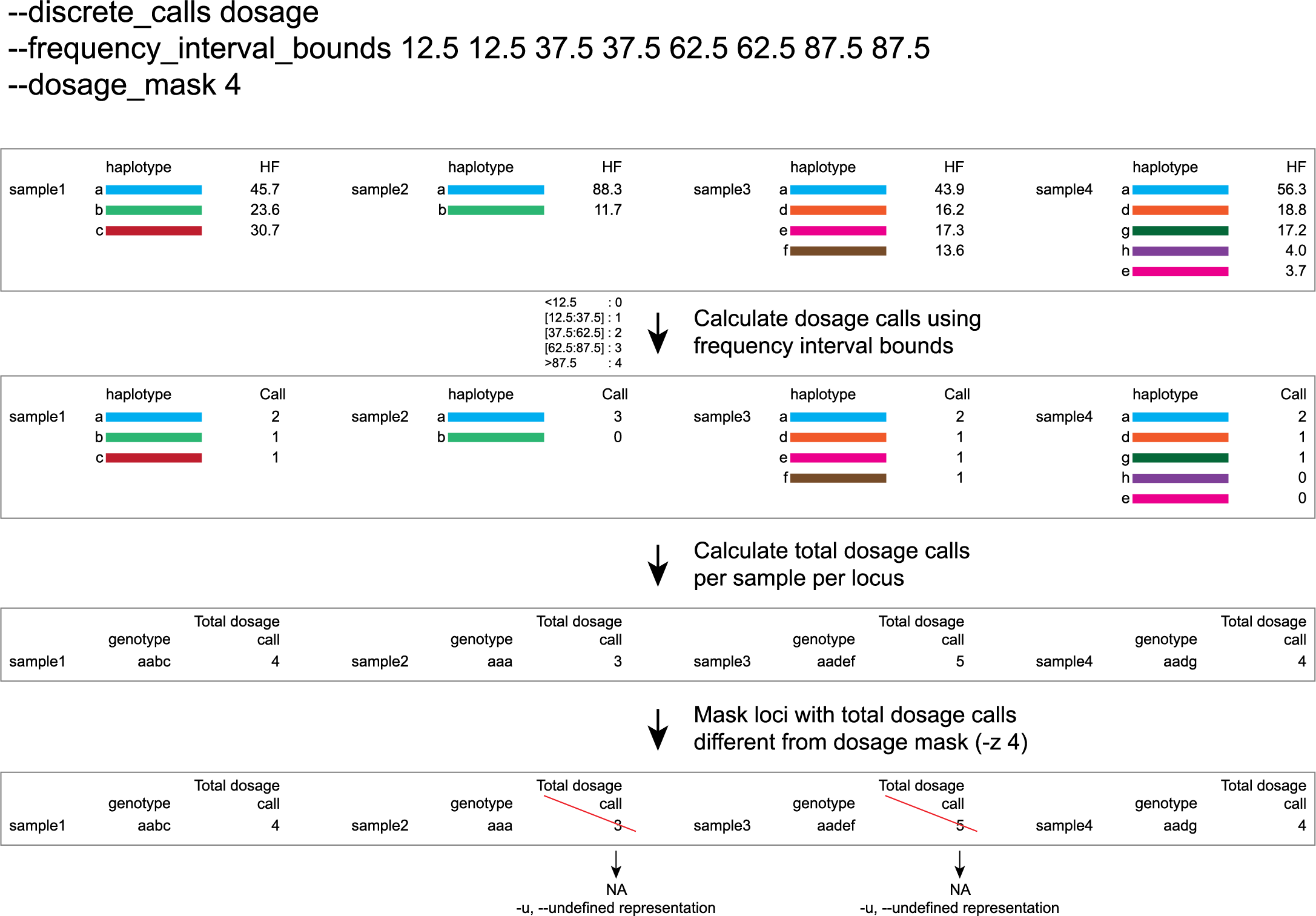
-e, –-discrete_calls ### (str) ### Set to “dominant” to transform haplotype frequency values into presence(1)/absence(0) calls per allele, or “dosage” to indicate the allele copy number.
-i, --frequency_interval_bounds ## Frequency interval bounds for classifying the read frequencies into discrete calls. Custom thresholds can be defined by passing one or more space-separated integers or floats which represent relative frequencies in percentage. For dominant calling, one value should be specified. For dosage calling, an even total number of four or more thresholds should be specified. Defaults are used by passing either “diploid”, “triploid”, or “tetraploid”. The default value for dominant calling (see discrete_calls argument) is 10, regardless if “diploid”, “triploid” or “tetraploid” is used. For dosage calling, the default for diploids is “10 10 90 90”, for triploids “12.5 12.5 50.0 50.0 87.5 87.5”, and for tetraploids “12.5 12.5 37.5 37.5 62.5 62.5 87.5 87.5”.
-z, --dosage_mask ### (int) ### Mask dosage calls in the loci for which the total dosage call for a given locus at a given sample differs from the defined value. For example, in diploid organisms the total dosage call must be 2, in triploid organisms the total dosage call must be 3, and in tetraploids the total dosage call must be 4 [default no masking].
--locus_correctness ######## (int) ### Threshold value: % of samples with locus correctness. Create a new GFF file defining only the loci that were correctly dosage called (-z) in at least the defined percentage of samples [default no filtering].
--allele_coded_genotype_matrix ######## (store_true) ### Create a new genotype matrix in which the haplotypes are transformed to their allele-coded representation. The allele-coded representation is a more compact way to represent the haplotypes, in which each haplotype is represented by a combination of its alleles. This can be useful for downstream analyses that require a more compact representation of the haplotypes, such as population genetic analyses or association studies.
--frequency_interval_bounds in practical examples and additional information on the dosage mask:
discrete dosage calls for diploids (0/1/2)
Use this option if you want to customize discrete calling thresholds. Haplotype calls with frequency below the lowerbound percentage are considered “not detected” and receive dosage `0´. Haplotype calls with a frequency between the lowerbound and the next percentage are considered heterozygous and receive haplotype dosage `1´. Haplotype calls with frequency above the upperbound percentage are considered homozygous and scored as haplotype dosage `2´. default <10, [10:90], >90 . Should be written with spaces between percentages, percentages may be written as floats or as integers [10 10 90 90].
e.g. --discrete_calls dosage --frequency_interval_bounds 10 10 90 90 translates to: haplotype frequency < 10% = 0, haplotype frequency > 10% & < 90% = 1, haplotype frequency > 90% = 2.
Graphical examples of these thresholds can be found in these tabs.
discrete dominant calls for diploids (0/1)
LowerBound frequency for dominant call haplotypes. Haplotypes with frequency above this percentage are scored as dominant present haplotype [10].
e.g. --discrete_calls dominant --frequency_interval_bounds 10 translates to: haplotype frequency < 10% = 0, haplotype frequency > 10% = 1
Graphical examples of these thresholds can be found in these tabs.
discrete dosage calls for triploids (0/1/2/3)
Use this option if you want to customize discrete calling thresholds, haplotype calls with frequency below the lowerbound percentage are considered not detected and receive dosage `0´ . Haplotype calls with frequency between the lowerbound and next percentage are considered present in 1 out of 3 alleles and scored as haplotype dosage `1´ , haplotype frequencies in the next frequency interval are scored as haplotype dosage `2´ . Haplotype calls with frequency above the upperbound percentage are considered homozygous and scored as haplotype dosage `3´ . Should be written with spaces between percentages, percentages may be written as floats or as integers [12.5 12.5 50.0 50.0 87.5 87.5].
e.g. --discrete_calls dosage --frequency_interval_bounds 12.5 12.5 50.0 50.0 87.5 87.5 translates to: haplotype frequency < 12.5% = 0, haplotype frequency > 12.5% & < 50% = 1, haplotype frequency > 50% & < 87.5% = 2, haplotype frequency > 87.5% = 3.
Graphical examples of these thresholds can be found in these tabs.
discrete dominant calls for triploids (0/1)
LowerBound frequency for dominant call haplotypes. Haplotypes with frequency above this percentage are scored as dominant present haplotype [10].
e.g. --discrete_calls dominant --frequency_interval_bounds 10 translates to: haplotype frequency < 10% = 0, haplotype frequency > 10% = 1.
Graphical examples of these thresholds can be found in these tabs.
discrete dosage calls for tetraploids (0/1/2/3/4)
Use this option if you want to customize discrete calling thresholds, haplotype calls with frequency below the lowerbound percentage are considered not detected and receive dosage `0´ . Haplotype calls with frequency between the lowerbound and next percentage are considered present in 1 out of 4 alleles and scored as haplotype dosage `1´ , haplotype frequencies in the next frequency interval are scored as haplotype dosage `2´ , and so on. Haplotype calls with frequency above the upperbound percentage are considered homozygous and scored as haplotype dosage `4´ default <12.5, [12.5:37.5], [37.5:62.5], [62.5:87.5], >87.5 . Should be written with spaces between percentages, percentages may be written as floats or as integers [12.5 12.5 37.5 37.5 62.5 62.5 87.5 87.5].
e.g. --discrete_calls dosage --frequency_interval_bounds 12.5 12.5 37.5 37.5 62.5 62.5 87.5 87.5 translates to: haplotype frequency < 12.5% = 0, haplotype frequency > 12.5% & < 37.5% = 1, haplotype frequency > 37.5% & < 62.5% = 2, haplotype frequency > 62.5% & < 87.5% = 3, haplotype frequency > 87.5% = 4.
Graphical examples of these thresholds can be found in these tabs.
discrete dominant calls for tetraploids (0/1)
LowerBound frequency for dominant call haplotypes. Haplotypes with frequency above this percentage are scored as dominant present haplotype [10].
e.g. --discrete_calls dominant --frequency_interval_bounds 10 translates to: haplotype frequency < 10% = 0, haplotype frequency > 10% = 1.
Graphical examples of these thresholds can be found in these tabs.
-z is an additional mask specifically for dosage calls in individuals. It masks loci within samples from the dataset (replaced by -u or --undefined_representation) based on total dosage calls (= total allele count calculated from haplotype frequencies using frequency interval bounds).locus |
dosage |
total dosage call |
number of unique alleles |
|||
|---|---|---|---|---|---|---|
. |
a |
b |
c |
d |
. |
. |
aaaa |
4 |
0 |
0 |
0 |
4 |
1 |
aaab |
3 |
1 |
0 |
0 |
4 |
2 |
aabb |
2 |
2 |
0 |
0 |
4 |
2 |
abcc |
1 |
1 |
2 |
0 |
4 |
3 |
abcd |
1 |
1 |
1 |
1 |
4 |
4 |
-z evaluates the total dosage call against the expected number of alleles (2 in diploids, 4 in tetraploids), but does not consider the number of unique alleles.-f (minimum haplotype frequency), --frequency_interval_bounds and -z (dosage_mask).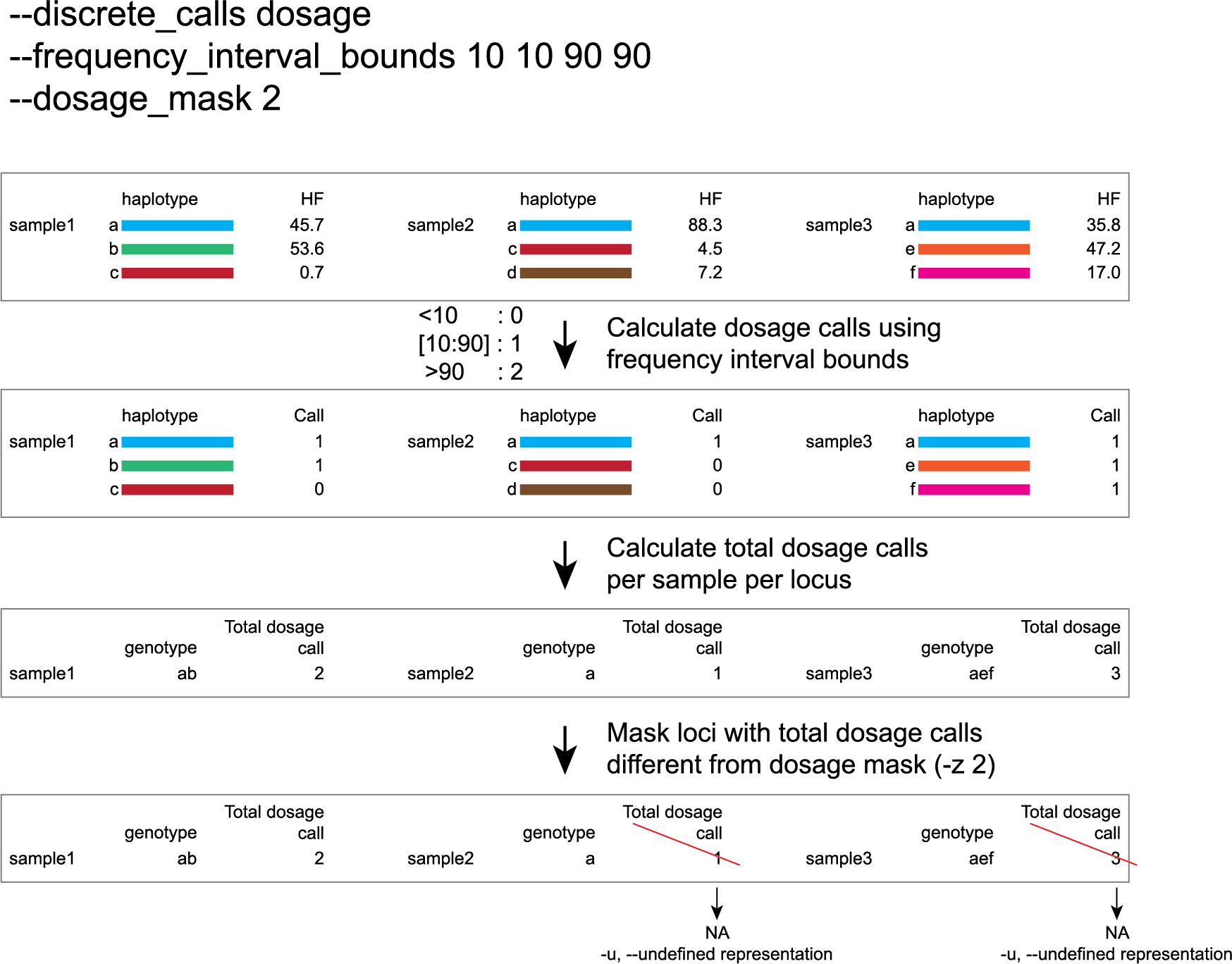
-f (minimum haplotype frequency) is especially useful to reduce the number of masked calls across the sample set.-f, the other haplotype values would have been recalculated and the total dosage would have become 2 (haplotype aa).--frequency_interval_bounds can be adjusted to fit the experimental data based on the haplotype frequency graphs in order to reduce the number of within-sample loci filtered out by --dosage_mask.Example commands
Pools
smap haplotype-window /location/of/RefGenome.fasta /location/of/borders.gff /directory/with/BAMs/ /directory/with/FASTQfiles/ --min_read_count 30 -f 2 -m 1 -u "" -p 8 --min_distinct_haplotypes 2
smap haplotype-window /location/of/RefGenome.fasta /location/of/borders.gff /directory/with/BAMs/ /directory/with/FASTQfiles/ --min_read_count 30 -f 2 -m 1 -u "" -p 8 --min_distinct_haplotypes 2
Individuals
smap haplotype-window /location/of/RefGenome.fasta /location/of/borders.gff /directory/with/BAMs/ /directory/with/FASTQfiles/ --min_read_count 10 --discrete_calls dominant --frequency_interval_bounds 10 -f 5 -u "" -p 8 --min_distinct_haplotypes 2
smap haplotype-window /location/of/RefGenome.fasta /location/of/borders.gff /directory/with/BAMs/ /directory/with/FASTQfiles/ --min_read_count 10 --discrete_calls dosage --frequency_interval_bounds 10 10 90 90 -f 5 -u "" --dosage_mask 2 -p 8 --min_distinct_haplotypes 2
smap haplotype-window /location/of/RefGenome.fasta /location/of/borders.gff /directory/with/BAMs/ /directory/with/FASTQfiles/ --min_read_count 15 --discrete_calls dominant --frequency_interval_bounds 10 -f 5 -u "" -p 8 --min_distinct_haplotypes 2
smap haplotype-window /location/of/RefGenome.fasta /location/of/borders.gff /directory/with/BAMs/ /directory/with/FASTQfiles/ --min_read_count 15 --discrete_calls dosage --frequency_interval_bounds 12.5 12.5 50.0 50.0 87.5 87.5 -f 5 -u "" --dosage_mask 3 -p 8 --min_distinct_haplotypes 2
smap haplotype-window /location/of/RefGenome.fasta /location/of/borders.gff /directory/with/BAMs/ /directory/with/FASTQfiles/ --min_read_count 20 --discrete_calls dominant --frequency_interval_bounds 10 -f 5 -u "" -p 8 --min_distinct_haplotypes 2
smap haplotype-window /location/of/RefGenome.fasta /location/of/borders.gff /directory/with/BAMs/ /directory/with/FASTQfiles/ --min_read_count 20 --discrete_calls dosage --frequency_interval_bounds 12.5 12.5 37.5 37.5 62.5 62.5 87.5 87.5 -f 5 -u "" --dosage_mask 4 -p 8 --min_distinct_haplotypes 2
Output
Tabular output
By default, SMAP haplotype-window will return two .tsv files.
haplotype counts
counts_cx_fx_mx.tsv (with x the value per option used in the analysis) contains the read counts (-c) and haplotype frequency (-f) filtered and/or masked (-m) read counts per haplotype per locus as defined in the BED file from SMAP delineate.
This is the file structure:
Reference
Locus
Haplotypes
Sample1
Sample2
Sample..
Chr1
Window_1
ACGTCGTCGC
60
13
34
Chr1
Window_1
ACGTCGTCAC
19
90
51
Chr1
Window_2
GCTCATCG
70
63
87
Chr1
Window_2
GCTCTCG
108
22
134
relative haplotype frequency
haplotypes_cx_fx_mx.tsv contains the relative frequency per haplotype per locus in sample (based on the corresponding count table: counts_cx_fx_mx.tsv). The transformation to relative frequency per locus-sample combination inherently normalizes for differences in total number of mapped reads across samples, and differences in amplification efficiency across loci. This is the file structure:
Reference
Locus
Haplotypes
Sample1
Sample2
Sample..
Chr1
Window_1
ACGTCGTCGC
0.76
0.13
0.40
Chr1
Window_1
ACGTCGTCAC
0.24
0.87
0.60
Chr1
Window_2
GCTCATCG
0.39
0.74
0.39
Chr1
Window_2
GCTCTCG
0.61
0.26
0.61
Additionally freqs_unfiltered.tsv can be further filtered using the options-j(minimum distinct haplotypes) and-k(maximum distinct haplotypes), resulting in the file freqs_distinct_haplotypes_filter.tsv
--discrete_calls is used, the program will return three additional .tsv files. Their order of creation and content is shown in the scheme above.--frequency_interval_bounds. The total sum of discrete dosage calls is expected to be 2 in diploids and 4 in tetraploids.--dosage_filter to remove loci per sample with an unexpected number of haplotype calls in haplotypes_cx_fx_mx_total_discrete_calls.tsv. The expected number of calls is set with option -z [use 2 for diploids, 4 for tetraploids].