How It Works
Workflow of SMAP haplotype-window
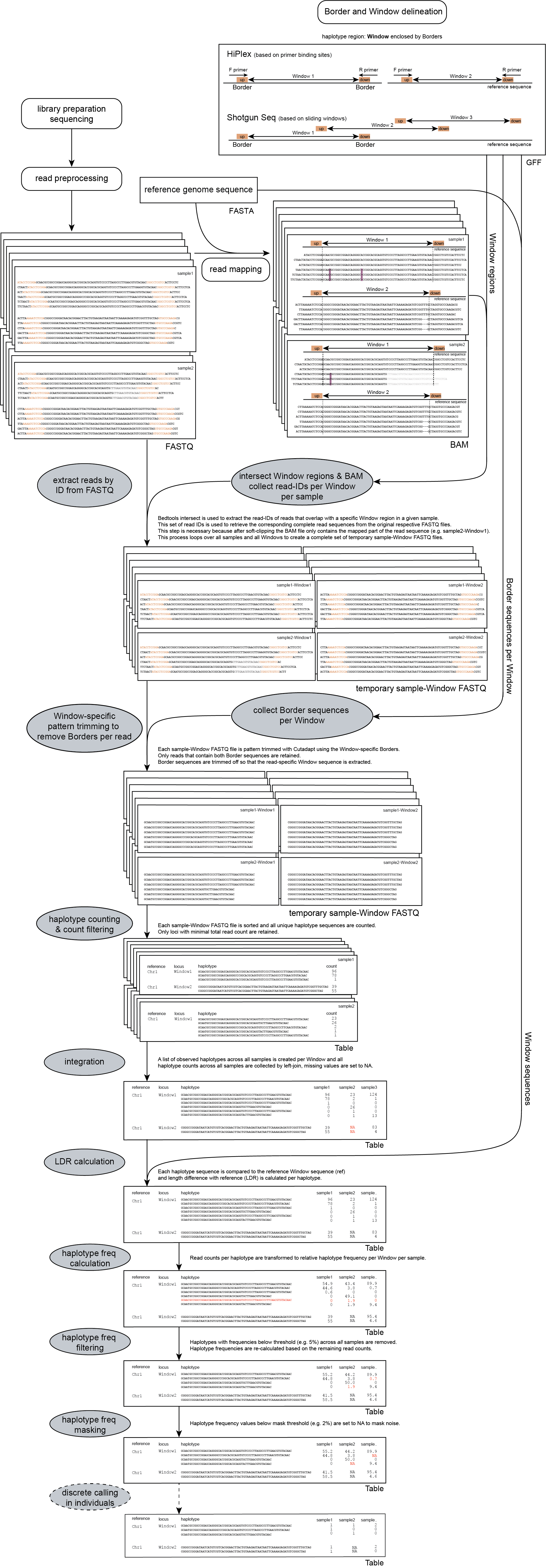
The FASTA file containing the reference sequence.
1. Name of the sequence in the reference that contains the Window.2. Source of the feature. [SMAP haplotype-window].3. Feature type. Because in SMAP haplotype-window pairs of Borders define Windows, two feature types are used: Border_upstream and Border_downstream. Each line in the GFF is one of those borders. Borders always come in pairs.4. The start coordinate of the Border region [in the 1-based GFF coordinate system].5. The end coordinate of the Border region [in the 1-based GFF coordinate system, value must always be higher than column 4].8. Score. Irrelevant for SMAP haplotype-window [.].7. Orientation of the Border [always +].8. Phase. Irrelevant for SMAP haplotype-window [.].9. Attributes of the Border, the field 'NAME=' is required. This field is used to pair Borders (by exact 'NAME=' matching), and define the corresponding Window regions. The field Name must be unique for each Window and will be used to name loci in the haplotype frequency tables.
For HiPlex data it is advised to use the 5-10 nucleotides on the 3’ of the primer binding site, where they flank the Window (to extract the sequence read region inbetween the primers).
ACD11
SMAP
CRISPR_border_up
124
133
.
+
.
NAME=ACD11_1
ACD11
SMAP
CRISPR_border_down
223
232
.
+
.
NAME=ACD11_1
ACD11
SMAP
CRISPR_border_up
864
873
.
+
.
NAME=ACD11_2
ACD11
SMAP
CRISPR_border_down
970
979
.
+
.
NAME=ACD11_2
ACD11
SMAP
CRISPR_border_up
4273
4282
.
+
.
NAME=ACD11_3
ACD11
SMAP
CRISPR_border_down
4393
4402
.
+
.
NAME=ACD11_3
AGD2
SMAP
CRISPR_border_up
726
735
.
+
.
NAME=AGD2_1
AGD2
SMAP
CRISPR_border_down
821
830
.
+
.
NAME=AGD2_1
AGD2
SMAP
CRISPR_border_up
4047
4056
.
+
.
NAME=AGD2_2
AGD2
SMAP
CRISPR_border_down
4154
4163
.
+
.
NAME=AGD2_2
Chr1
SMAP
CRISPR_border_up
1
10
.
+
.
NAME=Chr1_window_1
Chr1
SMAP
CRISPR_border_down
61
70
.
+
.
NAME=Chr1_window_1
Chr1
SMAP
CRISPR_border_up
21
30
.
+
.
NAME=Chr1_window_2
Chr1
SMAP
CRISPR_border_down
81
90
.
+
.
NAME=Chr1_window_2
Chr1
SMAP
CRISPR_border_up
41
50
.
+
.
NAME=Chr1_window_3
Chr1
SMAP
CRISPR_border_down
101
110
.
+
.
NAME=Chr1_window_3
Chr2
SMAP
CRISPR_border_up
61
70
.
+
.
NAME=Chr2_window_1
Chr2
SMAP
CRISPR_border_down
121
130
.
+
.
NAME=Chr2_window_1
Chr2
SMAP
CRISPR_border_up
81
90
.
+
.
NAME=Chr2_window_2
Chr2
SMAP
CRISPR_border_down
141
150
.
+
.
NAME=Chr2_window_2
A set of FASTQ files with reads that need to be haplotyped.
A set of BAM files made with BWA-MEM using the respective reference sequence and FASTQ files.
CRISPR/Cas extension of SMAP haplotype-window
A specific extension of the SMAP haplotype-window workflow for CRISPR data can be invoked using the optional command --guides.
If CRISPR/Cas genome editing was performed by stable transformation with a CRISPR/gRNA delivery vector, then the presence of the gRNA cassette in the delivery vector may be detected in the transformed genome. Primers can be designed on the vector sequence to amplify the gRNA sequence in the gRNA expression cassette, and Border regions can be positioned directly flanking the 20 bp gRNA sequence. The haplotype of that ‘locus’ that is then detected is effectively a copy of the gRNA sequence incorporated into the transformed genome. These primers can be included in the HiPlex primer set used to screen for the genomic target loci. SMAP haplotype-window can assign gRNA vector-derived reads to the respective target loci, if the user provides a FASTA file with the target loci names as identifiers and the 20 bp gRNA as sequence. In this way, genome-edited haplotypes at genomic target loci can be detected in parallel to the gRNAs that cause them, for any number of loci and any number of samples.
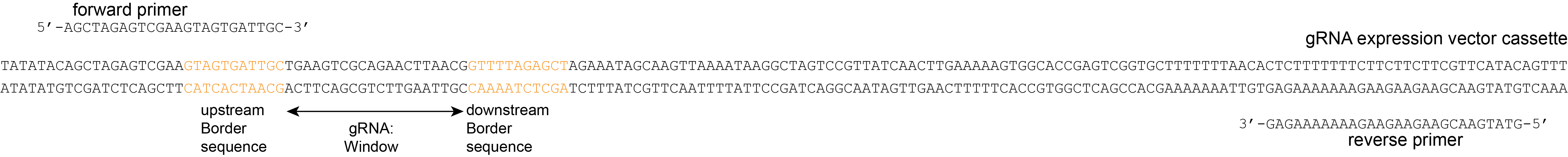
Example of gRNA sequences FASTA:
>AT1G07650_1_gRNA_001 |
|
TGAAGTCGCAGAACTTAACG |
|
>AT1G07650_1_gRNA_002 |
|
CTGAAGTCGCAGAACTTAAC |
Example of output file with diverse genome-edited haplotypes at genomic target loci and corresponding gRNA. By sorting on the fourth column (Target) in any output .tsv file, it is possible to arrange all the target loci with their corresponding gRNAs. Note that the standard output of SMAP haplotype-window can be further annotated by SMAP effect-prediction, for instance as the length difference with the reference, or even with the effect of the mutation on the predicted protein, in case candidate genes are used as reference sequence.
Reference |
Locus |
Haplotypes |
Target |
Sample1 |
Sample2 |
Sample3 |
Sample4 |
Sample5 |
Sample6 |
Sample7 |
|---|---|---|---|---|---|---|---|---|---|---|
AT1G07650 |
AT1G07650_1 |
GAGCTCTGAAGTCGCAGAACTTAACAGGCATTGTCCCTCCAGAATTCTCTAAGCTTCGTCACCTTAAAGTTTTG |
AT1G07650_1 |
100 |
100 |
100 |
100 |
100 |
100 |
|
AT1G07650 |
AT1G07650_2 |
AAGTGATAATAATTTCACTGGACCAATACCAGATTTCATCAGCAATTGGACAAGAATACTGAAACTGTACGATCTATTCTTT |
AT1G07650_2 |
100 |
100 |
100 |
100 |
100 |
100 |
100 |
AT1G07650 |
AT1G07650_3 |
CTTGTGAAGCTATATGGATGTTGTGTTGAAGGAAACCAATTGATATTGGTGTATGAGTACTTGGAGAACAACTGTCTA |
AT1G07650_3 |
100 |
100 |
100 |
100 |
100 |
100 |
100 |
AT2G02780 |
AT2G02780_1 |
CTTAGCTCTAATTTCATCTCTGGGAAGATTCCAGAAGAGATTGTGTCTTTGAAGAATCTGAAAAGCCTTGTTTTA |
AT2G02780_1 |
100 |
100 |
100 |
100 |
100 |
100 |
100 |
AT2G02780 |
AT2G02780_2 |
CATTGAAGAACAACTCCTTTAGATCCAAGATTCCAGAACAGATCAAGAAGCTGAATAACCTTCAAAGTTTAGACCTTTCT |
AT2G02780_2 |
100 |
100 |
100 |
100 |
100 |
100 |
100 |
AT2G02780 |
AT2G02780_3 |
TTTCTGAGTGTAGGACGTGTACCACAGACAATGAGATCTGCAGTAGATTGGTTTGCCACCGTACCGCGTTTTCTCCTTGGAG |
AT2G02780_3 |
6.22 |
6.12 |
|||||
AT2G02780 |
AT2G02780_3 |
TTTCTGAGTGTAGGACGTGTACCACAGACAATGAGATCTGCAGTGATTGGTTTGCCACCGTACCGCGTTTTCTCCTTGGAG |
AT2G02780_3 |
73.88 |
54.69 |
100 |
100 |
100 |
100 |
100 |
AT2G02780 |
AT2G02780_3 |
TTTCTGAGTGTAGGACGTGTACCACAGACAATGAGATCTGCAGTTGATTGGTTTGCCACCGTACCGCGTTTTCTCCTTGGAG |
AT2G02780_3 |
19.92 |
39.22 |
|||||
AT2G16250 |
AT2G16250_1 |
AGCGTTACCGGGGACTATACCTGAGTGGTTTGGTGTTAGTTTGTTGGCATTGGAAGTATTGGATCTTAGTTCGTGT |
AT2G16250_1 |
100 |
100 |
100 |
100 |
100 |
100 |
100 |
AT3G03770 |
AT3G03770_1 |
ACGCTTATACTCGACGAGAATATGTTTTCTGGTGAGTTACCCGGATTGGATTGATTCTTTGCCGAGTTTAGCTGTGTTGAGCTTGAG |
AT3G03770_1 |
2.22 |
||||||
AT3G03770 |
AT3G03770_1 |
ACGCTTATACTCGACGAGAATATGTTTTCTGGTGAGTTACCGAGATTGGATTGATTCTTTGCCGAGTTTAGCTGTGTTGAGCTTGAG |
AT3G03770_1 |
9.46 |
15.87 |
|||||
AT3G03770 |
AT3G03770_1 |
ACGCTTATACTCGACGAGAATATGTTTTCTGGTGAGTTACCGATTGGATTGATTCTTTGCCGAGTTTAGCTGTGTTGAGCTTGAG |
AT3G03770_1 |
10.81 |
23.62 |
|||||
AT3G03770 |
AT3G03770_1 |
ACGCTTATACTCGACGAGAATATGTTTTCTGGTGAGTTACCGGATTGGATTGATTCTTTGCCGAGTTTAGCTGTGTTGAGCTTGAG |
AT3G03770_1 |
72.06 |
39.84 |
100 |
100 |
100 |
100 |
100 |
AT3G03770 |
AT3G03770_1 |
ACGCTTATACTCGACGAGAATATGTTTTCTGGTGAGTTACCGTGATTGGATTGATTCTTTGCCGAGTTTAGCTGTGTTGAGCTTGAG |
AT3G03770_1 |
7.66 |
18.44 |
|||||
AT3G03770 |
AT3G03770_2 |
TGGATCTTTCCTACAATACATTCGTTGGTCCATTTCCTACTTCCTTGATGTCTCTTCCCGCGATAACTTACTTGAACA |
AT3G03770_2 |
100 |
100 |
100 |
100 |
100 |
100 |
100 |
AT3G03770 |
AT3G03770_3 |
TTTTCATTGTTCTTTTCAGATTTATAGAGGGAGATTGAAAGATGGATCCTTTGATGGCAATTAGGTGTCTGAA |
AT3G03770_3 |
7.94 |
14.58 |
|||||
AT3G03770 |
AT3G03770_3 |
TTTTCATTGTTCTTTTCAGATTTATAGAGGGAGATTGAAAGATGGATCCTTTGTGGCAATTAGGTGTCTGAA |
AT3G03770_3 |
42.09 |
9.28 |
100 |
100 |
100 |
100 |
100 |
AT3G03770 |
AT3G03770_3 |
TTTTCATTGTTCTTTTCAGATTTATAGAGGGAGATTGAAAGATGGATCCTTTGTTGGCAATTAGGTGTCTGAA |
AT3G03770_3 |
50 |
76.19 |
|||||
AT3G08680 |
AT3G08680_1 |
TATCCCTCCCGTCCTTTCTCATCGCCTCGTTAATCTTGATCTCTCCGCCAACTCGCTCTCGGGAAACATTCCCACGAGTCTACAA |
AT3G08680_1 |
100 |
100 |
100 |
100 |
100 |
100 |
100 |
AT3G08680 |
AT3G08680_2 |
TCTCCTTCACCGACAACACCAACAGAAGGTCCTGGTACAACCAATATAGGTCGTGGTACCGCCAAAAAAGTTCTCTCCACTGGTGCTATTGT |
AT3G08680_2 |
100 |
100 |
100 |
100 |
100 |
100 |
100 |
AT3G08680 |
AT3G08680_3 |
AGAAGTAGCAGCTGGAAAGAGGGAGTTCGAGCAGCAGATGGAAGCCGTGGGAAGGATCAGTCCACACGTGAAT |
AT3G08680_3 |
1.14 |
1.3 |
|||||
AT3G08680 |
AT3G08680_3 |
AGAAGTAGCAGCTGGGAAACGGGAGTTCGAGCAGCAGATGGAAGCCGTGGGAAGGATCAGTCCACACGTGAAT |
AT3G08680_3 |
100 |
100 |
98.88 |
100 |
100 |
100 |
98.75 |
AT3G13065 |
AT3G13065_1 |
TCTCGTTTTCTGTTTCTGTAGAAAAGTATCTGGACGTGGACTCAGTGGATCTTTAGGTTACCAGCTTGGAAA |
AT3G13065_1 |
100 |
100 |
100 |
100 |
100 |
100 |
100 |
AT3G24660 |
AT3G24660_1 |
GTTTTGCCTCCATCGATTTGGAACCTCTGTGATAAGCTTGTCTCTTTCAAGATTCATGGTAATAACTTGTCTGGGGTTTTGCC |
AT3G24660_1 |
100 |
100 |
100 |
100 |
100 |
100 |
100 |
AT3G24660 |
AT3G24660_2 |
GATTTTGGTGAGTCAAAGTTTGGAGCAGAATCTTTCGAAGGGAACAGTCCTAGCCTTTGTGGTTTGCCTTTGAAGC |
AT3G24660_2 |
100 |
100 |
100 |
100 |
36.25 |
100 |
100 |
AT3G24660 |
AT3G24660_2 |
GATTTTGGTGAGTCAAAGTTTGGAGCAGAATCTTTCGAAGGGAACAGTCCTAGGACTGCATGGTATCTTTGTGGTTTGCCTTTGAAGC |
AT3G24660_2 |
63.81 |
||||||
AT3G51740 |
AT3G51740_3 |
GATTCGTCATCAGAATCTTCTTGCACTAAGAGCTTACTACTTAGGACCTAAAGGAGAGAAGCTTCTCGTCTTTGATTACATGCCTAAAAGC |
AT3G51740_3 |
5.02 |
3.42 |
4.57 |
4.63 |
6.12 |
3.97 |
6.25 |
AT3G51740 |
AT3G51740_3 |
GATTCGTCATCAGAATCTTCTTGCACTAAGAGCTTACTACTTAGGACCTAAAGGAGAGAAGCTTCTCGTCTTTGATTACATGTCTAAAGGA |
AT3G51740_3 |
95.06 |
96.56 |
95.44 |
95.38 |
93.81 |
88.06 |
88.38 |
AT3G51740 |
AT3G51740_3 |
GATTCGTCATCAGAATCTTCTTGCACTAAGAGCTTACTACTTAGGACCTAAAGGGAGAGAAGCTTCTCGTCTTTGATTACATGTCTAAAGGA |
AT3G51740_3 |
7.94 |
5.36 |
|||||
AT5G20690 |
AT5G20690_2 |
TCCTCGGTACCAGAAACCTCGAAACAAGGCCGCAATAAACGCAATCATGGTGTCGATATCGCTTCTTCTCCTGTTCTTTATT |
AT5G20690_2 |
25.41 |
25.73 |
|||||
AT5G20690 |
AT5G20690_2 |
TCCTCGGTACCAGAAACCTCGAACAAGGCCGCAATAAACGCAATCATGGTGTCGATATCGCTTCTTCTCCTGTTCTTTATT |
AT5G20690_2 |
100 |
100 |
74.62 |
74.25 |
100 |
100 |
100 |
CRISPR_Vector |
gRNA |
ACTCATACACCAATATCAAT |
AT1G07650_3_gRNA_006 |
22.55 |
24.22 |
|||||
CRISPR_Vector |
gRNA |
ACAATGAGATCTGCAGTGAT |
AT2G02780_3_gRNA_077 |
45.09 |
46.81 |
|||||
CRISPR_Vector |
gRNA |
TTTGTTGGCATTGGAAGTAT |
AT2G16250_1_gRNA_080 |
61.53 |
||||||
CRISPR_Vector |
gRNA |
TTTCTGGTGAGTTACCGGAT |
AT3G03770_1_gRNA_109 |
54.88 |
53.19 |
|||||
CRISPR_Vector |
gRNA |
AAAGGCAAACCACAAAGGCT |
AT3G24660_2_gRNA_142 |
38.5 |
||||||
CRISPR_Vector |
gRNA |
ACGAGAAGCTTCTCTCCTTT |
AT3G51740_3_gRNA_150 |
29.88 |
30.45 |
|||||
CRISPR_Vector |
gRNA |
GGTACCAGAAACCTCGAACA |
AT5G20690_2_gRNA_213 |
23 |
21.62 |
|||||
CRISPR_Vector |
gRNA |
TAGAAGACGTTGACCATGCT |
gRNA_1 |
40.25 |
39.34 |
Reference |
Locus |
Haplotypes |
Target |
Sample1 |
Sample2 |
Sample3 |
Sample4 |
Sample5 |
Sample6 |
Sample7 |
|---|---|---|---|---|---|---|---|---|---|---|
AT1G07650 |
AT1G07650_1 |
GAGCTCTGAAGTCGCAGAACTTAACAGGCATTGTCCCTCCAGAATTCTCTAAGCTTCGTCACCTTAAAGTTTTG |
AT1G07650_1 |
100 |
100 |
100 |
100 |
100 |
100 |
|
AT1G07650 |
AT1G07650_2 |
AAGTGATAATAATTTCACTGGACCAATACCAGATTTCATCAGCAATTGGACAAGAATACTGAAACTGTACGATCTATTCTTT |
AT1G07650_2 |
100 |
100 |
100 |
100 |
100 |
100 |
100 |
AT1G07650 |
AT1G07650_3 |
CTTGTGAAGCTATATGGATGTTGTGTTGAAGGAAACCAATTGATATTGGTGTATGAGTACTTGGAGAACAACTGTCTA |
AT1G07650_3 |
100 |
100 |
100 |
100 |
100 |
100 |
100 |
CRISPR_Vector |
gRNA |
ACTCATACACCAATATCAAT |
AT1G07650_3_gRNA_006 |
22.55 |
24.22 |
|||||
AT2G02780 |
AT2G02780_1 |
CTTAGCTCTAATTTCATCTCTGGGAAGATTCCAGAAGAGATTGTGTCTTTGAAGAATCTGAAAAGCCTTGTTTTA |
AT2G02780_1 |
100 |
100 |
100 |
100 |
100 |
100 |
100 |
AT2G02780 |
AT2G02780_2 |
CATTGAAGAACAACTCCTTTAGATCCAAGATTCCAGAACAGATCAAGAAGCTGAATAACCTTCAAAGTTTAGACCTTTCT |
AT2G02780_2 |
100 |
100 |
100 |
100 |
100 |
100 |
100 |
AT2G02780 |
AT2G02780_3 |
TTTCTGAGTGTAGGACGTGTACCACAGACAATGAGATCTGCAGTAGATTGGTTTGCCACCGTACCGCGTTTTCTCCTTGGAG |
AT2G02780_3 |
6.22 |
6.12 |
|||||
AT2G02780 |
AT2G02780_3 |
TTTCTGAGTGTAGGACGTGTACCACAGACAATGAGATCTGCAGTGATTGGTTTGCCACCGTACCGCGTTTTCTCCTTGGAG |
AT2G02780_3 |
73.88 |
54.69 |
100 |
100 |
100 |
100 |
100 |
AT2G02780 |
AT2G02780_3 |
TTTCTGAGTGTAGGACGTGTACCACAGACAATGAGATCTGCAGTTGATTGGTTTGCCACCGTACCGCGTTTTCTCCTTGGAG |
AT2G02780_3 |
19.92 |
39.22 |
|||||
CRISPR_Vector |
gRNA |
ACAATGAGATCTGCAGTGAT |
AT2G02780_3_gRNA_077 |
45.09 |
46.81 |
|||||
AT2G16250 |
AT2G16250_1 |
AGCGTTACCGGGGACTATACCTGAGTGGTTTGGTGTTAGTTTGTTGGCATTGGAAGTATTGGATCTTAGTTCGTGT |
AT2G16250_1 |
100 |
100 |
100 |
100 |
100 |
100 |
100 |
CRISPR_Vector |
gRNA |
TTTGTTGGCATTGGAAGTAT |
AT2G16250_1_gRNA_080 |
61.53 |
||||||
AT3G03770 |
AT3G03770_1 |
ACGCTTATACTCGACGAGAATATGTTTTCTGGTGAGTTACCCGGATTGGATTGATTCTTTGCCGAGTTTAGCTGTGTTGAGCTTGAG |
AT3G03770_1 |
2.22 |
||||||
AT3G03770 |
AT3G03770_1 |
ACGCTTATACTCGACGAGAATATGTTTTCTGGTGAGTTACCGAGATTGGATTGATTCTTTGCCGAGTTTAGCTGTGTTGAGCTTGAG |
AT3G03770_1 |
9.46 |
15.87 |
|||||
AT3G03770 |
AT3G03770_1 |
ACGCTTATACTCGACGAGAATATGTTTTCTGGTGAGTTACCGATTGGATTGATTCTTTGCCGAGTTTAGCTGTGTTGAGCTTGAG |
AT3G03770_1 |
10.81 |
23.62 |
|||||
AT3G03770 |
AT3G03770_1 |
ACGCTTATACTCGACGAGAATATGTTTTCTGGTGAGTTACCGGATTGGATTGATTCTTTGCCGAGTTTAGCTGTGTTGAGCTTGAG |
AT3G03770_1 |
72.06 |
39.84 |
100 |
100 |
100 |
100 |
100 |
AT3G03770 |
AT3G03770_1 |
ACGCTTATACTCGACGAGAATATGTTTTCTGGTGAGTTACCGTGATTGGATTGATTCTTTGCCGAGTTTAGCTGTGTTGAGCTTGAG |
AT3G03770_1 |
7.66 |
18.44 |
|||||
CRISPR_Vector |
gRNA |
TTTCTGGTGAGTTACCGGAT |
AT3G03770_1_gRNA_109 |
54.88 |
53.19 |
|||||
AT3G03770 |
AT3G03770_2 |
TGGATCTTTCCTACAATACATTCGTTGGTCCATTTCCTACTTCCTTGATGTCTCTTCCCGCGATAACTTACTTGAACA |
AT3G03770_2 |
100 |
100 |
100 |
100 |
100 |
100 |
100 |
AT3G03770 |
AT3G03770_3 |
TTTTCATTGTTCTTTTCAGATTTATAGAGGGAGATTGAAAGATGGATCCTTTGATGGCAATTAGGTGTCTGAA |
AT3G03770_3 |
7.94 |
14.58 |
|||||
AT3G03770 |
AT3G03770_3 |
TTTTCATTGTTCTTTTCAGATTTATAGAGGGAGATTGAAAGATGGATCCTTTGTGGCAATTAGGTGTCTGAA |
AT3G03770_3 |
42.09 |
9.28 |
100 |
100 |
100 |
100 |
100 |
AT3G03770 |
AT3G03770_3 |
TTTTCATTGTTCTTTTCAGATTTATAGAGGGAGATTGAAAGATGGATCCTTTGTTGGCAATTAGGTGTCTGAA |
AT3G03770_3 |
50 |
76.19 |
|||||
AT3G08680 |
AT3G08680_1 |
TATCCCTCCCGTCCTTTCTCATCGCCTCGTTAATCTTGATCTCTCCGCCAACTCGCTCTCGGGAAACATTCCCACGAGTCTACAA |
AT3G08680_1 |
100 |
100 |
100 |
100 |
100 |
100 |
100 |
AT3G08680 |
AT3G08680_2 |
TCTCCTTCACCGACAACACCAACAGAAGGTCCTGGTACAACCAATATAGGTCGTGGTACCGCCAAAAAAGTTCTCTCCACTGGTGCTATTGT |
AT3G08680_2 |
100 |
100 |
100 |
100 |
100 |
100 |
100 |
AT3G08680 |
AT3G08680_3 |
AGAAGTAGCAGCTGGAAAGAGGGAGTTCGAGCAGCAGATGGAAGCCGTGGGAAGGATCAGTCCACACGTGAAT |
AT3G08680_3 |
1.14 |
1.3 |
|||||
AT3G08680 |
AT3G08680_3 |
AGAAGTAGCAGCTGGGAAACGGGAGTTCGAGCAGCAGATGGAAGCCGTGGGAAGGATCAGTCCACACGTGAAT |
AT3G08680_3 |
100 |
100 |
98.88 |
100 |
100 |
100 |
98.75 |
AT3G13065 |
AT3G13065_1 |
TCTCGTTTTCTGTTTCTGTAGAAAAGTATCTGGACGTGGACTCAGTGGATCTTTAGGTTACCAGCTTGGAAA |
AT3G13065_1 |
100 |
100 |
100 |
100 |
100 |
100 |
100 |
AT3G24660 |
AT3G24660_1 |
GTTTTGCCTCCATCGATTTGGAACCTCTGTGATAAGCTTGTCTCTTTCAAGATTCATGGTAATAACTTGTCTGGGGTTTTGCC |
AT3G24660_1 |
100 |
100 |
100 |
100 |
100 |
100 |
100 |
AT3G24660 |
AT3G24660_2 |
GATTTTGGTGAGTCAAAGTTTGGAGCAGAATCTTTCGAAGGGAACAGTCCTAGCCTTTGTGGTTTGCCTTTGAAGC |
AT3G24660_2 |
100 |
100 |
100 |
100 |
36.25 |
100 |
100 |
AT3G24660 |
AT3G24660_2 |
GATTTTGGTGAGTCAAAGTTTGGAGCAGAATCTTTCGAAGGGAACAGTCCTAGGACTGCATGGTATCTTTGTGGTTTGCCTTTGAAGC |
AT3G24660_2 |
63.81 |
||||||
CRISPR_Vector |
gRNA |
AAAGGCAAACCACAAAGGCT |
AT3G24660_2_gRNA_142 |
38.5 |
||||||
AT3G51740 |
AT3G51740_3 |
GATTCGTCATCAGAATCTTCTTGCACTAAGAGCTTACTACTTAGGACCTAAAGGAGAGAAGCTTCTCGTCTTTGATTACATGCCTAAAAGC |
AT3G51740_3 |
5.02 |
3.42 |
4.57 |
4.63 |
6.12 |
3.97 |
6.25 |
AT3G51740 |
AT3G51740_3 |
GATTCGTCATCAGAATCTTCTTGCACTAAGAGCTTACTACTTAGGACCTAAAGGAGAGAAGCTTCTCGTCTTTGATTACATGTCTAAAGGA |
AT3G51740_3 |
95.06 |
96.56 |
95.44 |
95.38 |
93.81 |
88.06 |
88.38 |
AT3G51740 |
AT3G51740_3 |
GATTCGTCATCAGAATCTTCTTGCACTAAGAGCTTACTACTTAGGACCTAAAGGGAGAGAAGCTTCTCGTCTTTGATTACATGTCTAAAGGA |
AT3G51740_3 |
7.94 |
5.36 |
|||||
CRISPR_Vector |
gRNA |
ACGAGAAGCTTCTCTCCTTT |
AT3G51740_3_gRNA_150 |
29.88 |
30.45 |
|||||
AT5G20690 |
AT5G20690_2 |
TCCTCGGTACCAGAAACCTCGAAACAAGGCCGCAATAAACGCAATCATGGTGTCGATATCGCTTCTTCTCCTGTTCTTTATT |
AT5G20690_2 |
25.41 |
25.73 |
|||||
AT5G20690 |
AT5G20690_2 |
TCCTCGGTACCAGAAACCTCGAACAAGGCCGCAATAAACGCAATCATGGTGTCGATATCGCTTCTTCTCCTGTTCTTTATT |
AT5G20690_2 |
100 |
100 |
74.62 |
74.25 |
100 |
100 |
100 |
CRISPR_Vector |
gRNA |
GGTACCAGAAACCTCGAACA |
AT5G20690_2_gRNA_213 |
23 |
21.62 |
|||||
CRISPR_Vector |
gRNA |
TAGAAGACGTTGACCATGCT |
gRNA_1 |
40.25 |
39.34 |