Recommendations & Troubleshooting
Guidelines for read preprocessing and mapping
Picking the right enzyme(s) for GBS library construction
GBS method optimization starts with choosing the best (combination of) enzymes for the species
Here, we first illustrate how to optimize the choice of restriction enzymes using empirical data on a small number of samples as a pilot experiment. We also illustrate a special case where genetic distance between reference genome and sample genome sequence influences the saturation curves. Then, we draw your attention to the importance of normalisation for sample pooling before multiplex library sequencing, and its evaluation using read depth saturation curves. Also, check out the relationship between read depth saturation and locus completeness across the sample set.
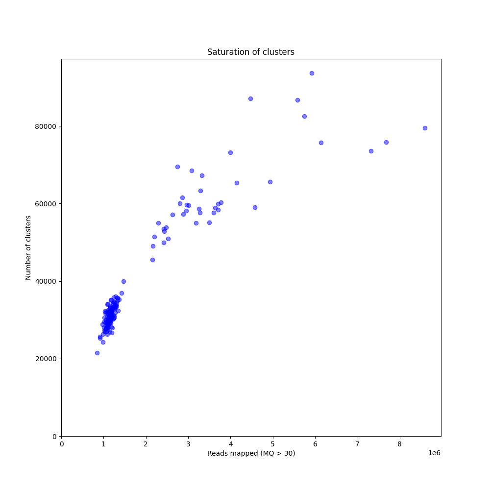
The saturation curve shows how many loci are detected in the reference sequence as a function of the number of reads mapped, and given the thresholds for read length, read depth, etc, used in SMAP delineate. The curve is constructed by sequencing GBS libraries to very high numbers of reads (more than eventually needed for routine screens), and then computationally subsampling incrementally larger fractions of the original .fastq files (1M, 2M, 3M, 4M reads, etc), as if only that number of reads were available per sample for read mapping. SMAP delineate is then run on the entire set of bam files. The curve clearly shows the typical non-linear relationship between the total number of reads per library and the increasing number of loci. At first, many regions of the genome are covered at relatively low read depth, close to the minimal read depth per locus threshold, and a small increase in total number of reads mapped (randomly distributed across all possible loci) quickly leads to an increase in the number of loci with read depth above the threshold. When a saturating number of reads has been reached per sample, the number of loci detected reaches a plateau and no further loci can be discovered, even if more reads are mapped. From that point onwards, reads are expected to map onto the same loci and increase the total read depth per locus. The ideal choice of enzymes is the combination that gives the maximal number of loci as plateau, with total number of reads per sample within budgetary limits.
The graph above compares saturation curves for four genotypes with differential genetic distance to the reference genome. The reference sequence used for all read mapping was generated using de novo assembly of whole-genome Illumina shotgun sequencing (WGS) of genotype R58, a heterozygous diploid individual. Genotype Y2 is a genetically different heterozygous diploid individual. F1 is a first generation progeny of a cross between R58 and Y2, and BC1 is a progeny of the backcross of an F1 individual and the parental R58 individual. So, the difference in the total number of loci detected in the four individuals can be explained by the similarity between the reference sequence and the genome complement per individual. First, all GBS reads generated in the R58 individual are expected to map onto the R58 reference sequence. The GBS library generated in the Y2 individual is expected to contain reads derived from a shared fraction of the genome sequence, and these can be mapped onto the R58 genome sequence. There are, however, also Y2-genome derived reads that can not map onto the R58 reference genome because the Y2-unique genome complement has not been assembled in the R58 reference sequence. So, while a similar total number of reads per individual is used for mapping, comparably less loci are identified in Y2 than in R58. The R58 x Y2 F1 progeny that contains half the genome complement of R58 and the other half of Y2, displays a saturation curve at intermediary number of loci per million reads mapped. The backcross BC1 (R58 x F1) is expected to contain 75% of the R58-genome complement and 25% of the Y2-genome complement and the BC1 saturation curve is indeed intermediary to that of the R58 and the F1 individual. Taken together, this illustrates that saturation curves (displaying how many loci are covered on the reference sequence per sample) can both be used to optimize the choice of restriction enzyme for GBS library construction and to estimate the required minimal number of reads per sample to reach saturation. It also shows that the choice of a representative reference sequence and a representative set of samples for pilot experiments is important.
Are we there yet? Validating saturation in actual sample sets
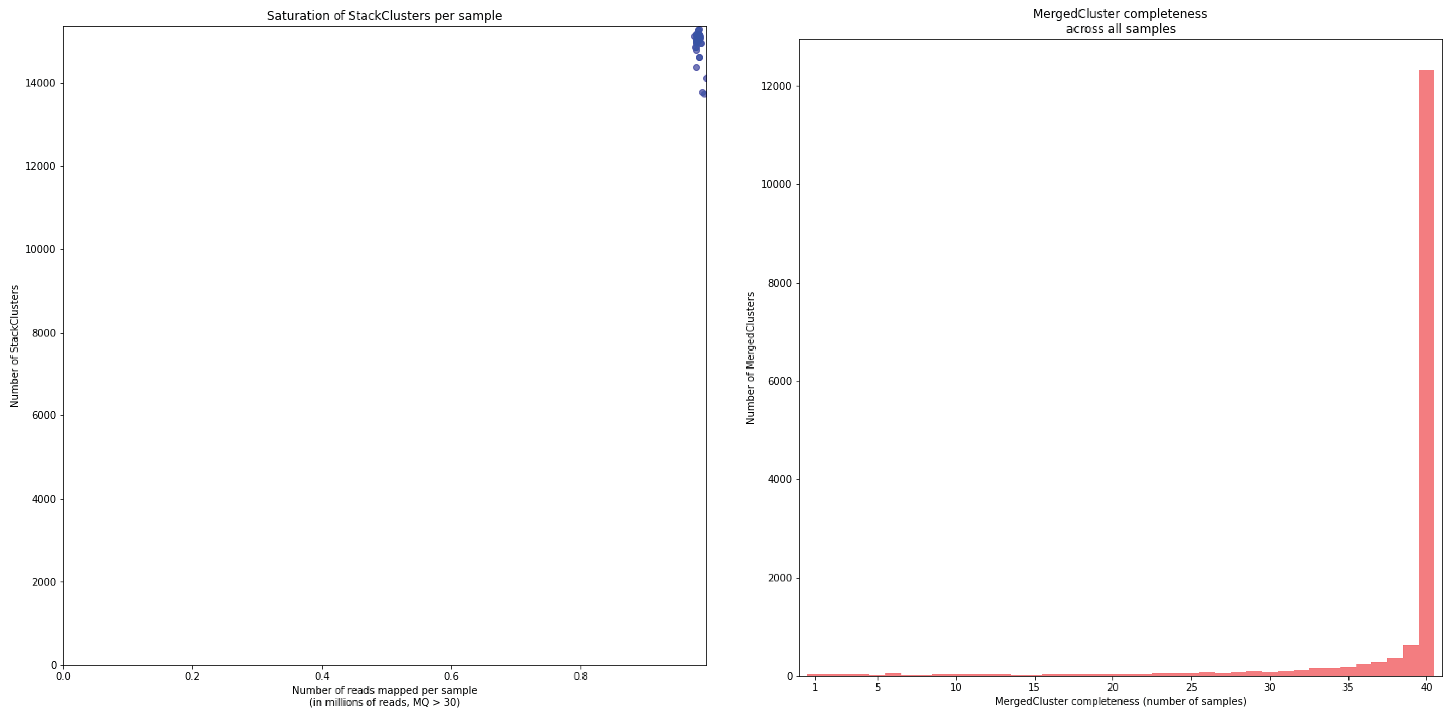
Perfect equally-normalized sample set with very few dropout samples. Samples with over-saturated read depth shows that adding more read depth per sample would hardly add any more loci to the final genotype table.
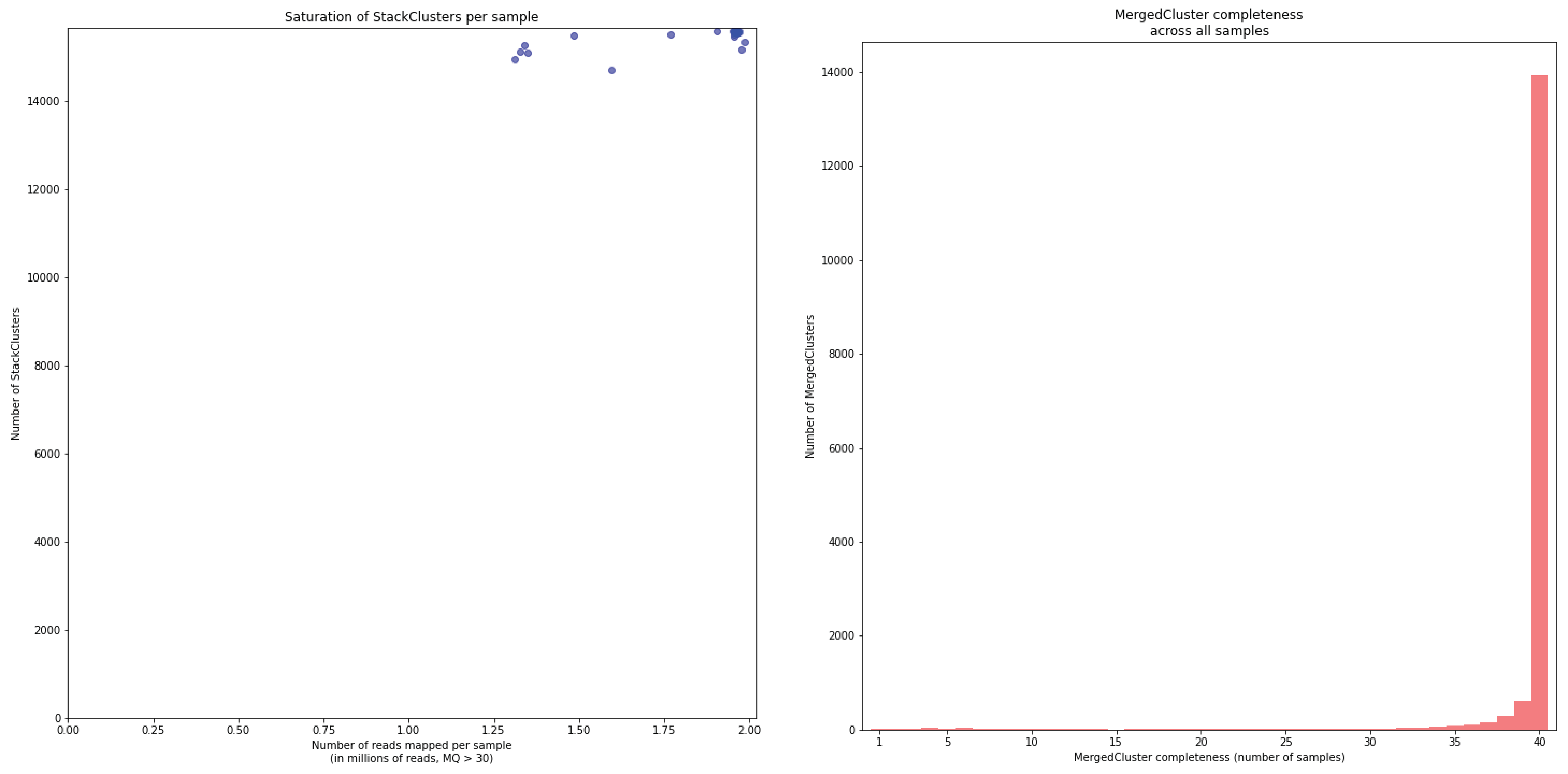
Poorly normalized sample set, with mostly non-saturated read depth per sample. Most samples populate the steep (highly non-saturated) part of the curve and the few more deeply sequenced samples reveal the projected plateau. Therefore, although the equally normalized bulk of the samples contains about the same number of StackClusters, these StackClusters are not necessarily originary from the same loci.
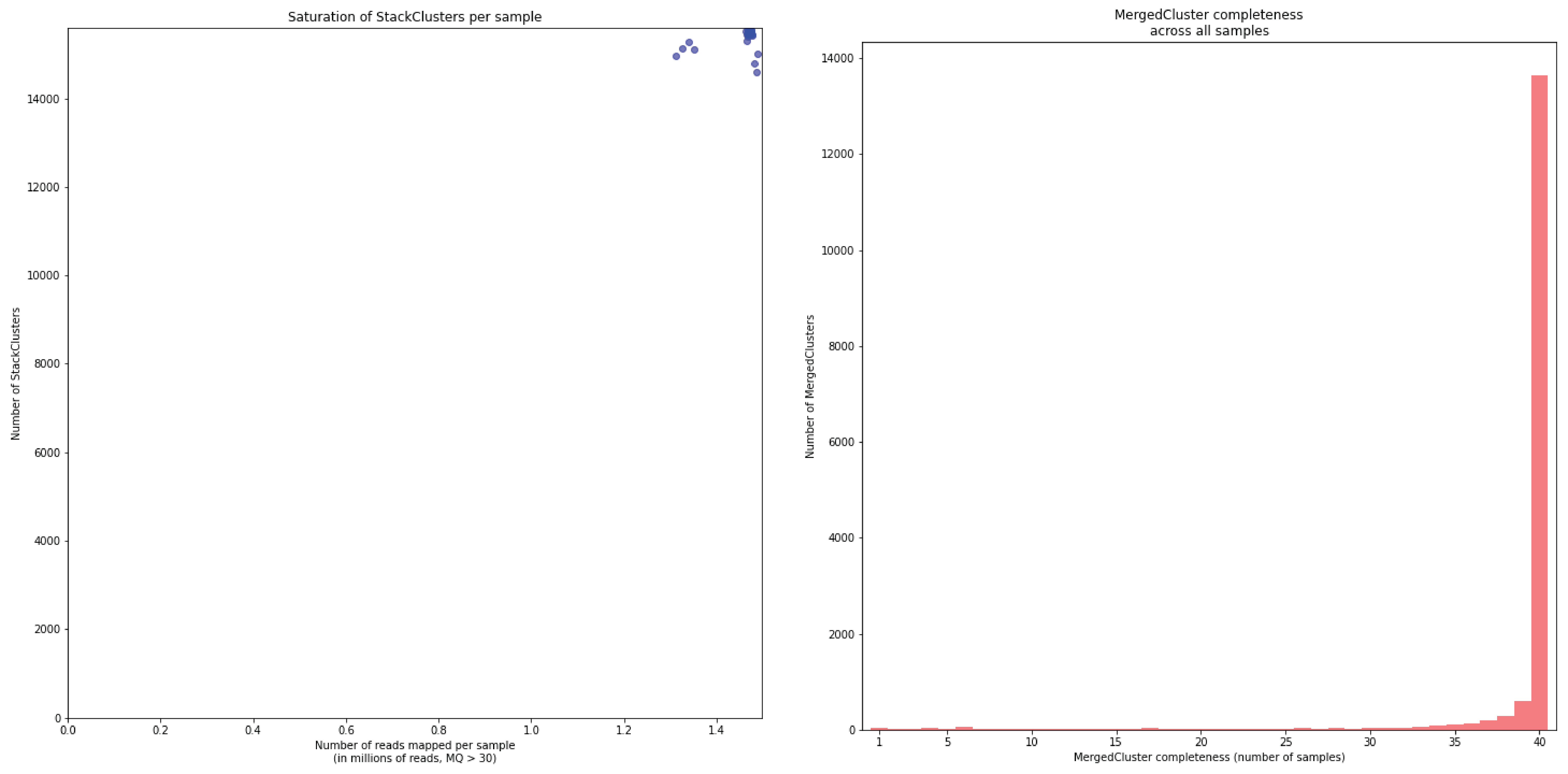
Equally normalized sample set, but non-saturated read depth per sample. The bulk of the samples are sequenced to about 1 M reads, and there are no drop-out samples, but the more deeply sequenced samples reveal that the maximum number of loci per sample has not been reached.
Please notice that apart from choosing a target number of reads per sample and corresponding expected number of loci during GBS method optimization, it is equally important to balance the number of reads per sample by sample-normalization during multiplex sequencing (equal amount per library loaded onto the sequencer). If, on average across the entire sample set, the number of reads per sample should be enough to reach the locus saturation plateau, but there is large variation in read number within the sample set, then (over)saturation is only reached for a fraction of the samples, while other samples are not sequenced to saturating read depth. This, in turn, will lead to missingness in the final genotype call table that can only be mitigated by sequencing individual drop-out samples to greater read depth until saturation is reached for all required samples.
Sources of locus incompleteness across sample sets
Bioinformatics analyses that compare reads mapped to a common reference to identify sequence variants require that sufficient reads are mapped to the same reference genome locations across sample sets. Here, as molecular markers are compared per locus and across all samples the information content of a given molecular marker depends on the completeness of locus observations across the sample set. We therefore define completeness as the fraction of the samples in which a given locus is observed, and analyse the distribution of completenes scores per locus across the entire sample set. GBS data critically suffers from incompleteness for two confounded reasons: both technical and biological aspects affect read mapping positions and read depth. So, it is important to first analyze if read mapping positions and read depth are consistent across the sample set, for the simple reason that if reads are not mapped to a given location, no variants can be identified in that sample, leading to missing data in the final sample-genotype call table.
In short, locus incompleteness can result from two main causes:
technical aspects, such as insufficient total number of reads per sample to reach locus saturation (see above).
biological aspects, such as the uniqueness of loci amplified from individual samples (because of a particular distribution of restriction sites in the genome of that sample versus any of the other samples in the set).
How to recognize the source of incompleteness in your data
The saturation curve and the completeness graph generated by SMAP delineate are the most important sources of information. If the saturation curve shows that all samples have been sequenced to saturating total read depth, this means that all technical limitations have been resolved and that sequencing samples to greater depth will not resolve incompleteness in genotype call tables. Please note that while all samples may display the same total number of loci per sample (plateau in the saturation curve), this does not mean that these loci have the same position on the genome across all samples. As genome sequence polymorphisms (InDels, SNPs) affect restriction sites, the actual genomic loci amplified as GBS-fragments also differ between individuals, and thus the derived read mapping locations. This is the reason that SMAP delineate compares the overlap between all loci across the sample set by creating MergedClusters and recording how many samples contribute to that MergedCluster across the sample set. This, literally, is the completeness score per locus.
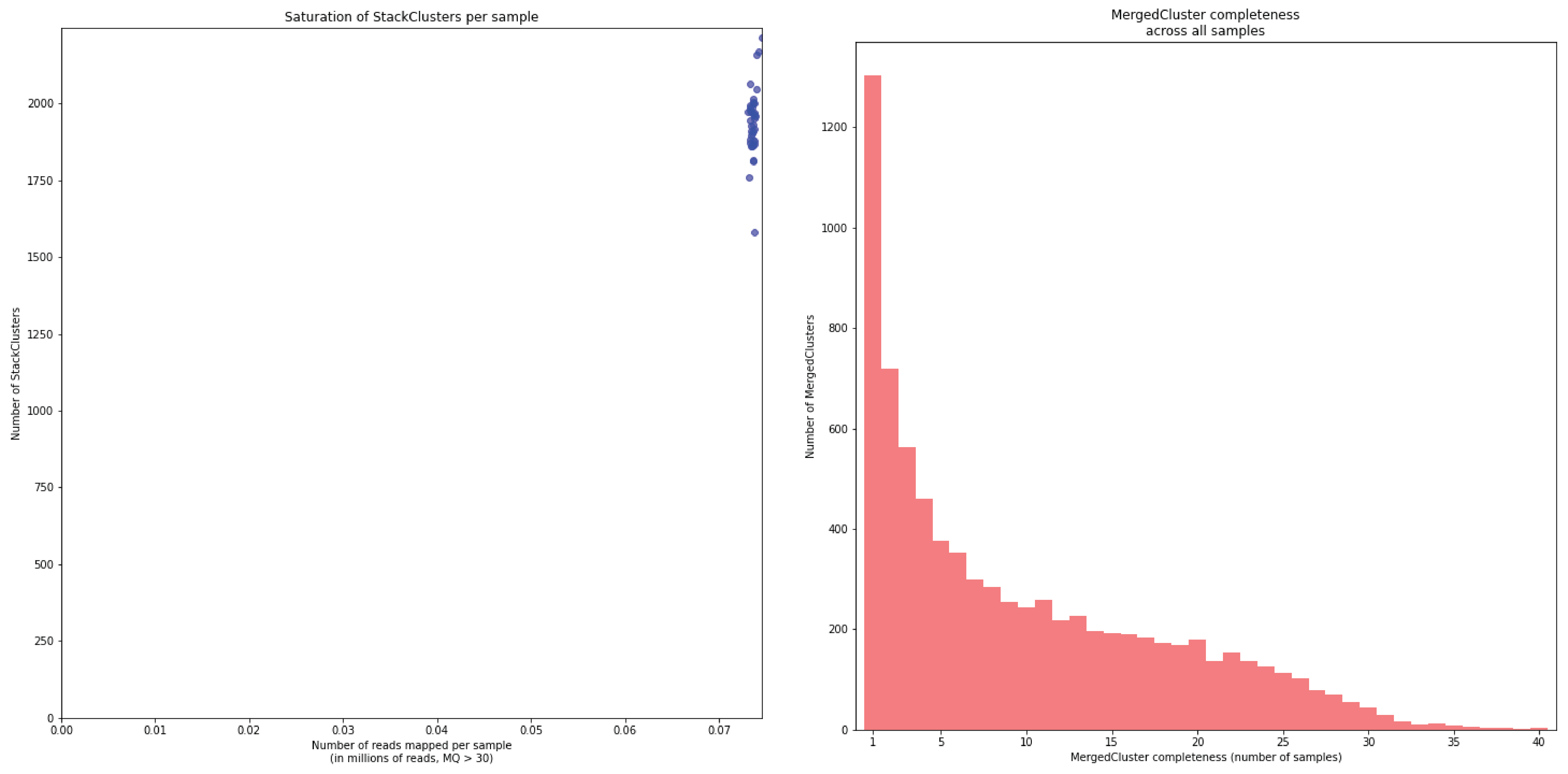
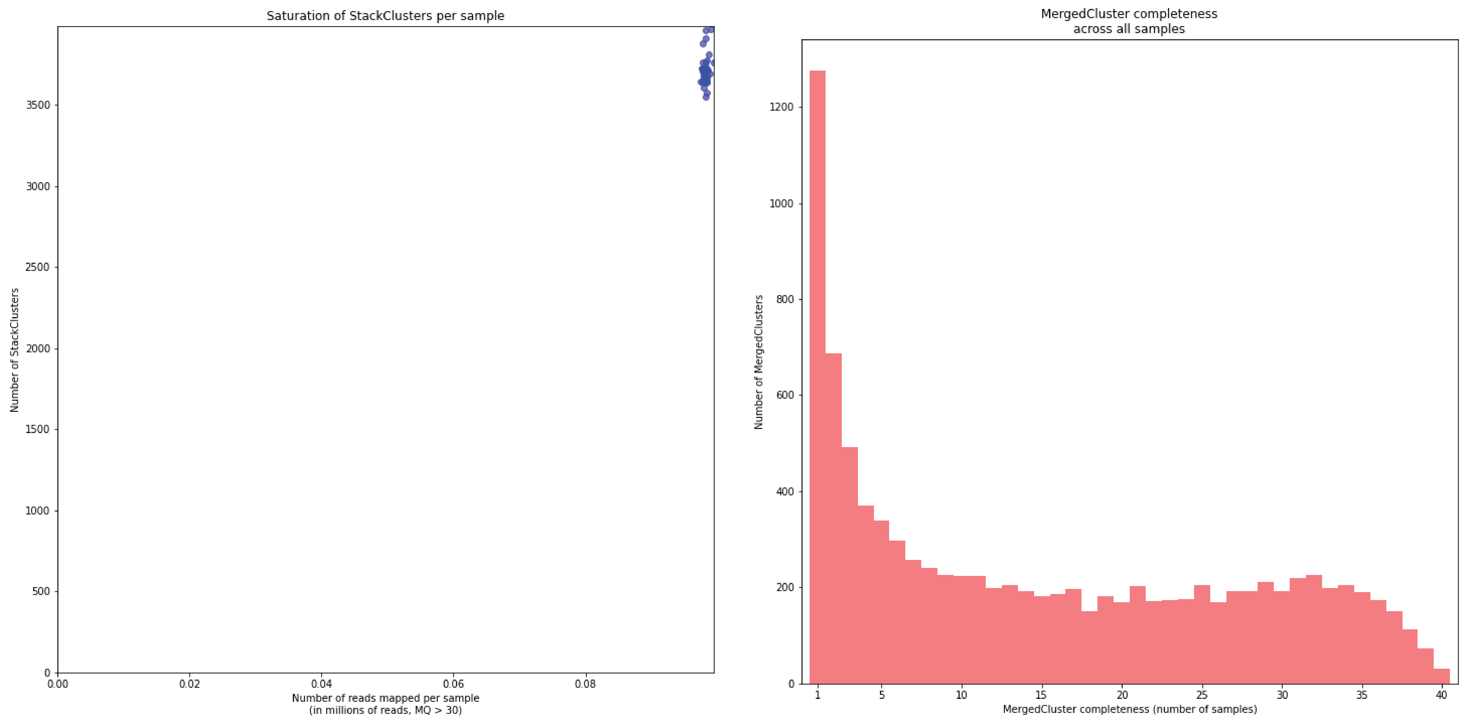
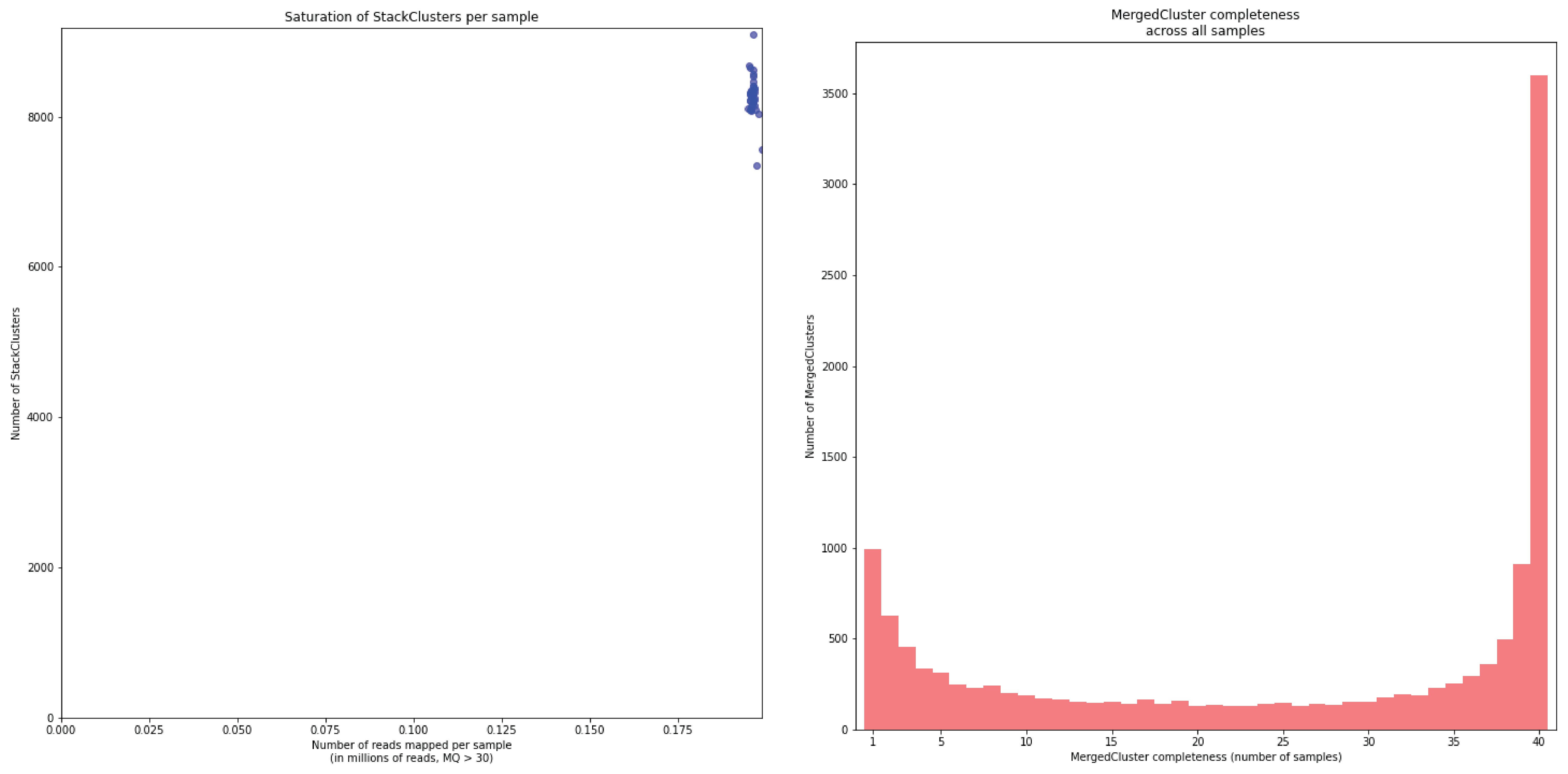
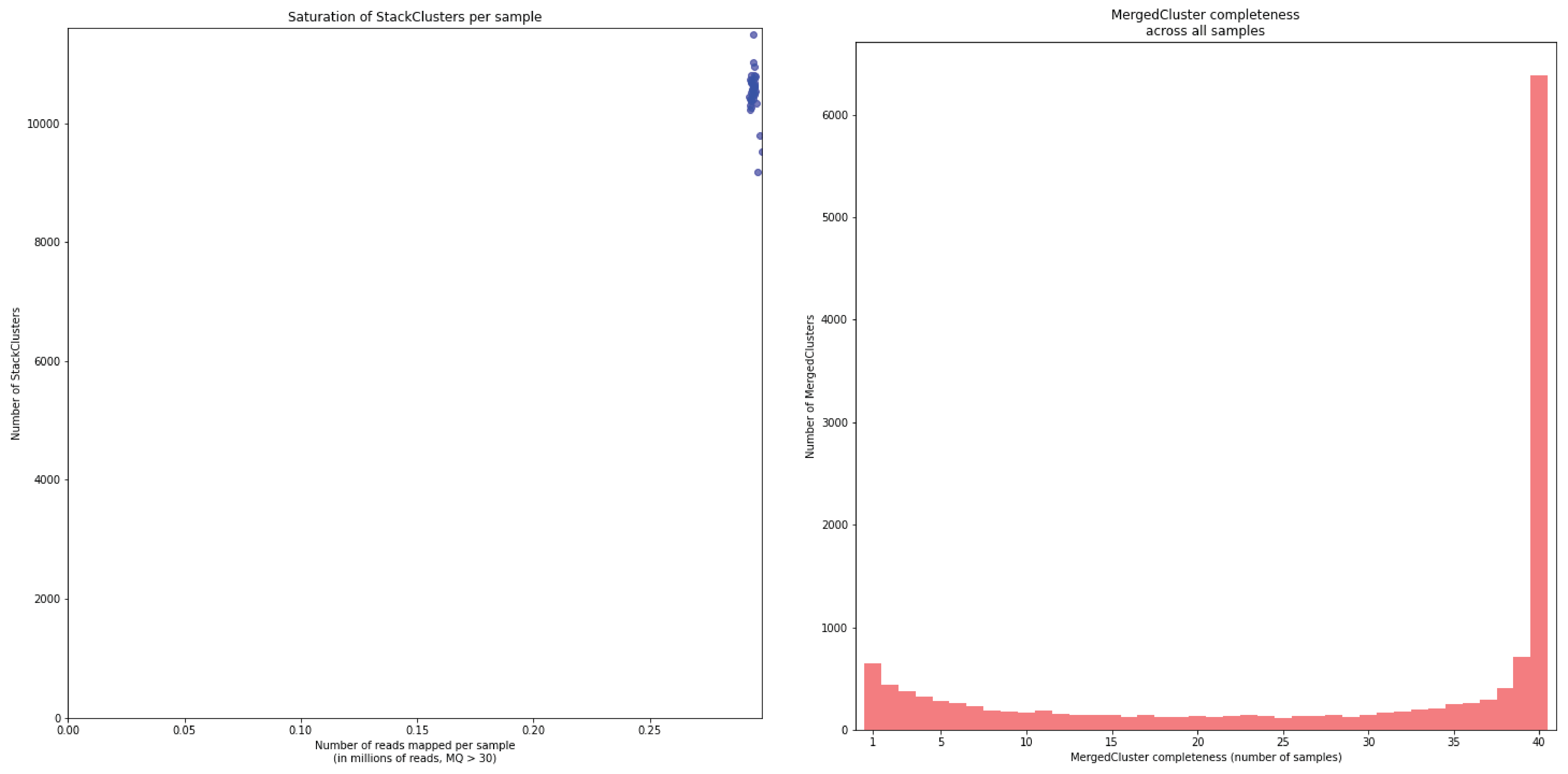
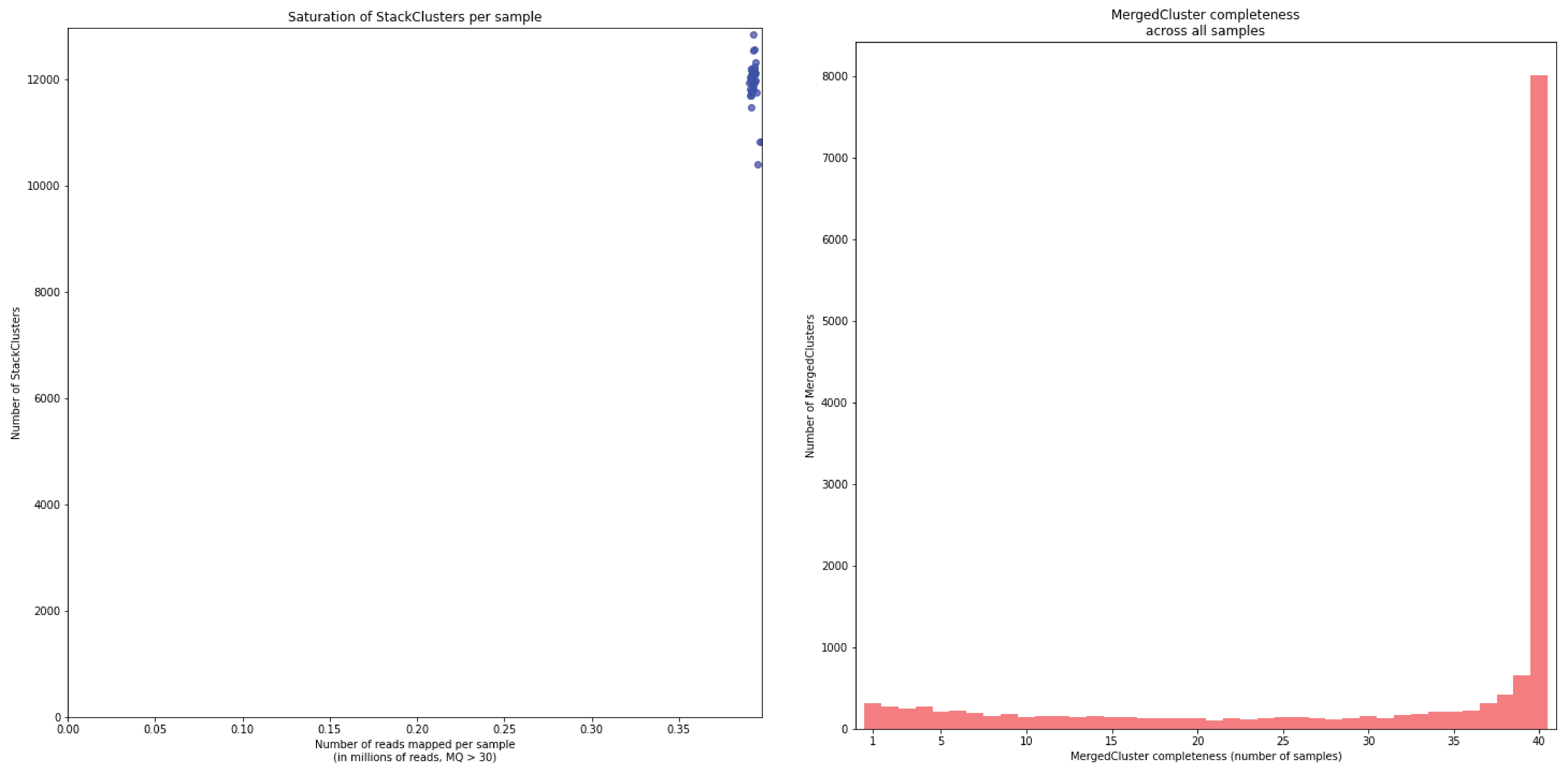
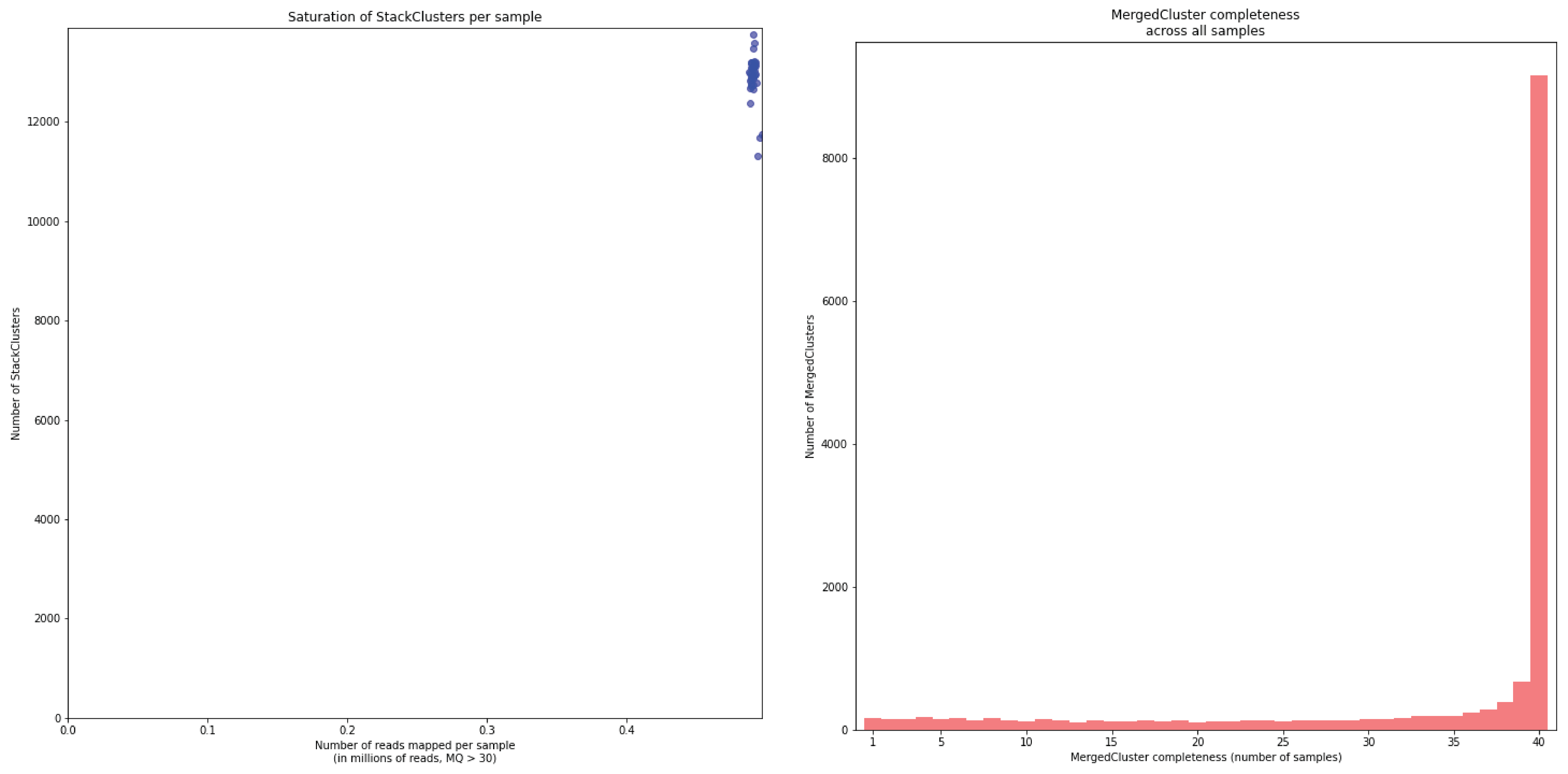
To illustrate this point, consider the relationship between saturation and completeness by comparing these curves (displayed the the tabs below) at increasing numbers of reads per sample across a set of 40 individuals. As total number of reads per sample increases from 0.1 M per sample to 1.5M per sample, the saturation curves show that mapping 1.5M reads per sample approaches saturation. Now compare the shift in the completeness distribution from strong left-hand skew (extreme incompleteness) towards right-hand skew: increasingly more loci are observed in which all samples have sufficient reads mapped for downstream genotype calling.
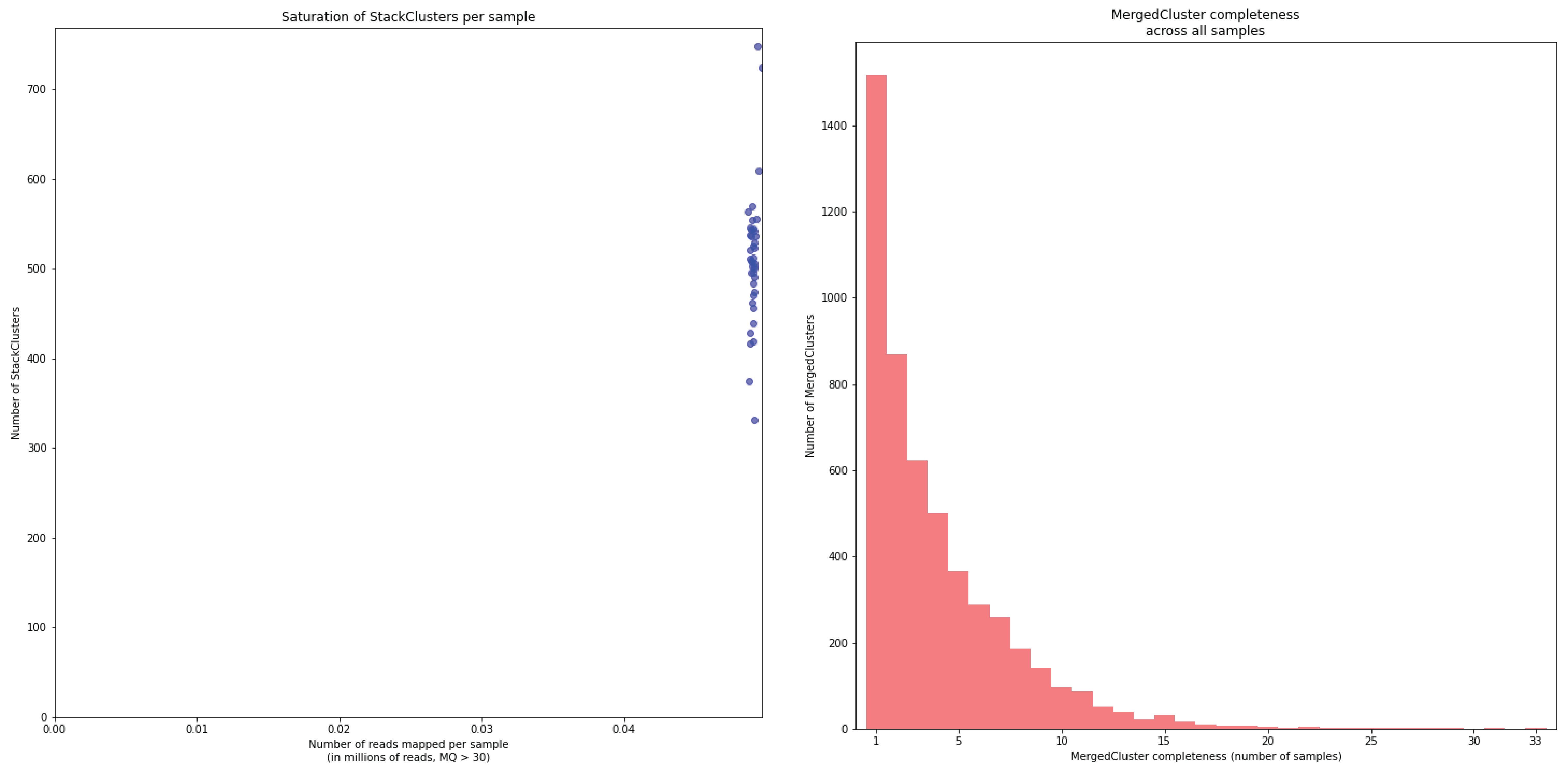
Note the increasing number of loci (y-axis) at increasing number of reads mapped.
Note the increasing number of loci (y-axis) at increasing number of reads mapped.
Note the increasing number of loci (y-axis) at increasing number of reads mapped.
Note the increasing number of loci (y-axis) at increasing number of reads mapped.
Note the increasing number of loci (y-axis) at increasing number of reads mapped.
Note the increasing number of loci (y-axis) at increasing number of reads mapped.
Note the increasing number of loci (y-axis) at increasing number of reads mapped.
Note the increasing number of loci (y-axis) at increasing number of reads mapped.
Note the increasing number of loci (y-axis) at increasing number of reads mapped.
In a sample set with low genetic diversity, the majority of loci are expected to be detected in all samples, if all samples have been sequenced to saturation. Notice that by 1 to 1.5 million preprocessed FASTQ reads the samples start spreading out in the Saturation curve due to samples not containing 1 million FASTQ reads. However the samples that do have more reads do not increase in number of StackClusters, indicating that the plateau has been reached.
Note the increasing number of loci (y-axis) at increasing number of reads mapped.
Note the increasing number of loci (y-axis) at increasing number of reads mapped.
Note the increasing number of loci (y-axis) at increasing number of reads mapped.
Note the increasing number of loci (y-axis) at increasing number of reads mapped.
Note the increasing number of loci (y-axis) at increasing number of reads mapped.
Note the increasing number of loci (y-axis) at increasing number of reads mapped.
Note the increasing number of loci (y-axis) at increasing number of reads mapped.
In a sample set with high genetic diversity, a substantial fraction of all loci is expected to be relatively unique to one or a few individuals and only a relatively small fraction of loci is commonly observed across all samples, even if all samples have been sequenced to saturation.
To merge or not to merge
If paired-end data is obtained, two stategies can be applied. The first strategy maps both reads separately, and processes the mapped reads into MergedClusters taking strandedness into account. The benefits are that more read mapping polymorphisms (SMAPs) are taken into account for haplotype calling and that long non-overlapping reads, that would not be merged and thus removed, are included in the analysis. The drawback is that multiple (partially overlapping, and potentially redundant) MergedClusters may be derived from a single locus, thus inflating the number of allelic markers, while essentially no additional genetic loci are covered (see How it works).
The second strategy first merges the forward and reverse read per GBS-amplified fragment, thus creating a longer single read. The benefit is that because the single resulting read may span more neighboring SNPs, thus extending the potential length of local haplotypes, removing the redundancy observed in separately mapped reads, and that read depth is maximal per locus (strandedness is not taken into account for delineating MergedClusters, see How it works). It is important to choose a particular minimal length of the overlap between the forward and reverse reads during the merging process.
Picking a minimum merging overlap length is a trade-off between sacrificing long loci, and removing incorrectly merged reads, it is recommended to at least use a merging overlap of 10 nucleotides to remove most of the incorrectly merged reads, see also Figure 6 in Magoč T. & Salzberg S., 2011.
Another point of attention is the error rate in the merging overlap allowed by the merging algorithm. In PEAR this error rate is controlled using the option -p, which when disabled can result in poorly merged reads with up to 30%-40% mismatches in the overlap region. GBprocesS uses the default value and avoids generating incorrecly merged reads.
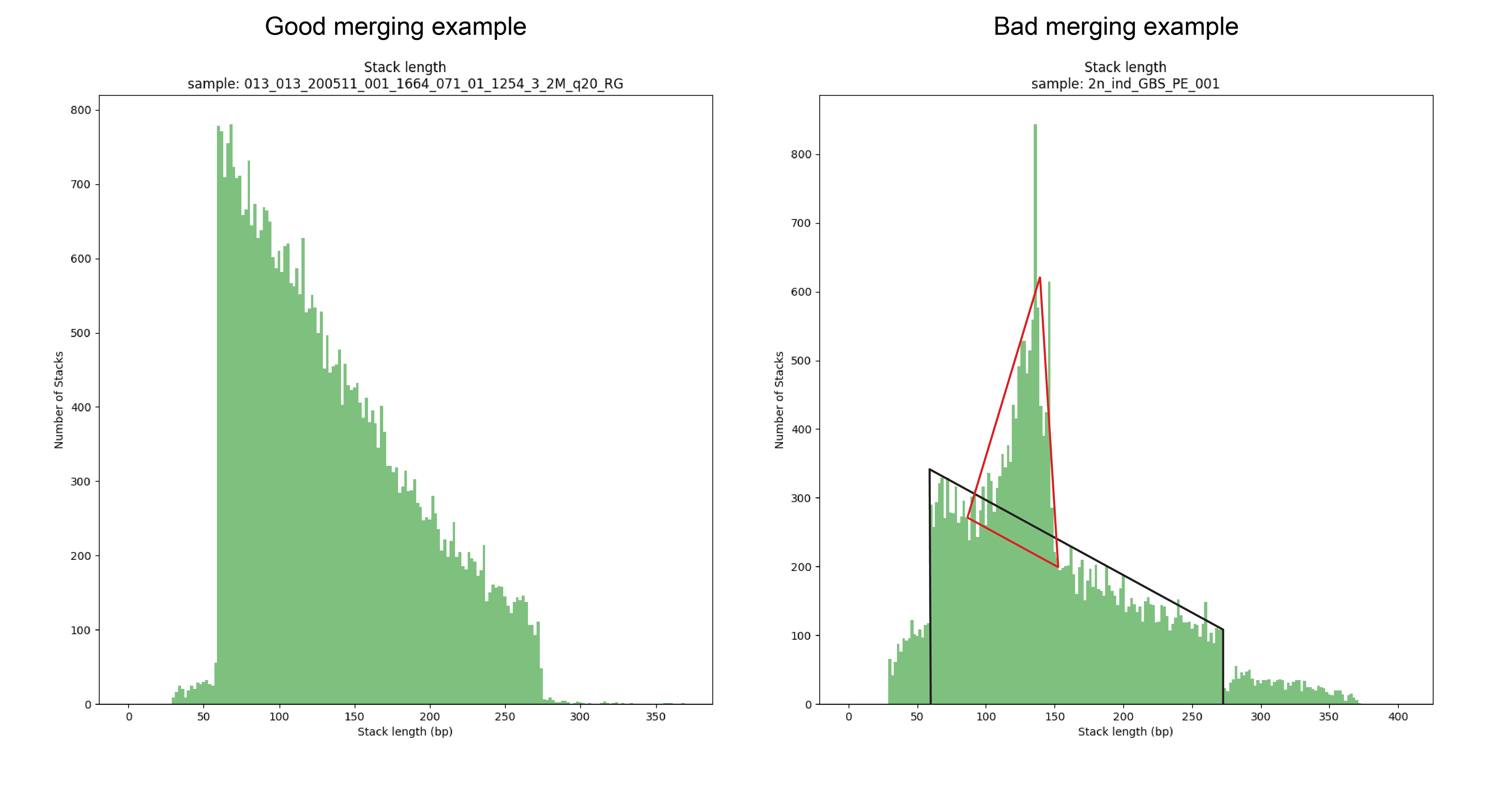
How to recognize the effect of inappropriate read merging in your data
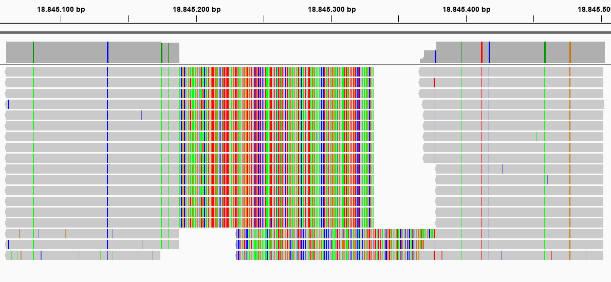
This first locus is approximately 450 bp long, and its reads should not have been merged. In the downstream mapped StackCluster, most reads are soft clipped (above) or hard clipped (below, hard clipped bases are not shown in IGV) on the exact same position; therefore not creating any false SMAPs. In the downstream mapped reads, the hard and soft clipping occurs differentially; creating two major Stacks (see upper dark grey bar), and therefore two SMAPs are created on the 5’ of the downstream mapped StackCluster where only one SMAP should occur (or none if the reads were not merged during read preprocessing, and thus excluded from mapping in the first place).
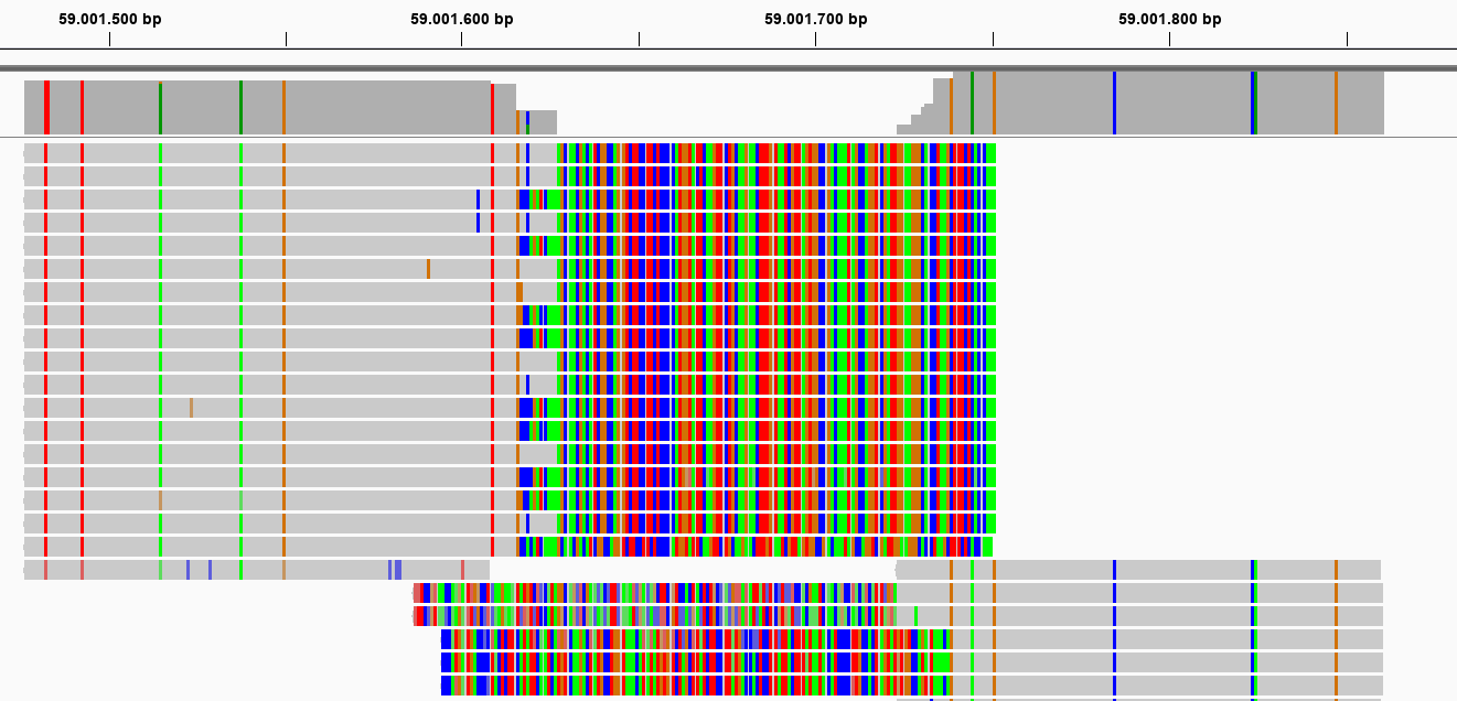
This second locus is approximately 400 bp long, and its reads should not have been merged (as there can be no overlap in 2x 136bp reads (after trimming) from opposite sides of a 400 bp fragment). In the upstream mapped StackCluster, 2 SMAPs are visible at the 3’ end of the mapping due to differential soft clipping. In the downstream mapped StackCluster, several different SMAPs are visible on the 5’ end of the mapping, but only based on few reads each.
How to resolve inappropriate read merging in your data
Repeat preprocessing with adjusted error rate in merging overlap
This first solution is to repeat the read preprocessing with GBprocesS with adjusted parameters. This is the most straightforward and effective procedure, but requires the most effort, as it includes repeating preprocessing and mapping of all data. Alternatively, it may be interesting to use the built-in parameters of SMAP delineate further discussed below to remove StackClusters derived from incorrectly merged reads and other errors.
Adequate Stack and StackCluster read depth filtering
Often, Stacks of incorrectly merged reads occur at low read depths, because of their differential merging and mapping. By incrementally increasing the Stack read depth minimum ( -x ) and StackCluster read depth minimum ( -c ) these incorrectly merged reads can easily be filtered out.
However, this comes at the cost of also excluding other good loci that are sequenced at shallow depth.
Adequate Stack Depth Fraction and Stacks per StackCluster values
Following ploidy, the expected relative abundance of Stacks in StackClusters is 50% for heterozygous diploid individuals and 25% for heterozygous tetraploid individuals. In reality, relative abundances follow a Gaussian distribution around these values. A SDF value of 10.0 for individuals for example would remove most incorrectly merged reads and other spurious errors.
For pools, it is harder to remove incorrectly merged reads using Stack Depth Fraction, as the maximal number of alleles on a locus is defined by the diversity and the number of samples in a pool.
Lastly, the number of Stacks per StackCluster can be controlled using the option -l. In individuals, the maximum number of Stacks per StackCluster should be equal to the ploidy, and in pools this depends on the diversity and number of samples in the pool.
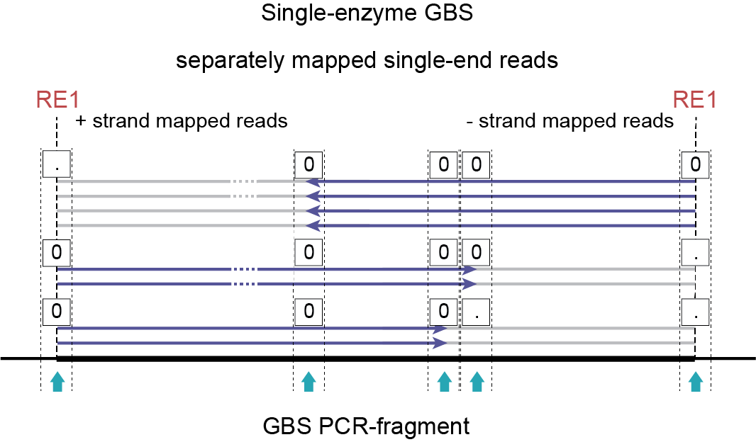
Why Strandedness is considered for single reads
`Single reads´ include single-enzyme or double-enzyme single-end reads or separately mapped paired-end reads (see How it works for more information). The explanation below is tailored to single-enzyme single-end reads but can be applied on the three other combinations.
How reads cover polymorphisms within the PCR-fragment region
Consider a diploid heterozygous locus defined by one deletion located in the upstream region (left hand side) of the fragment:
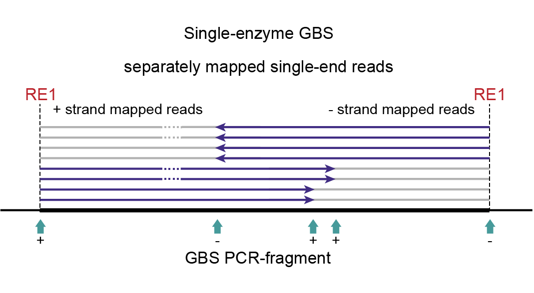
As a heterozygous locus, half of the PCR-amplified molecules are expected to carry the deletion, the other half of the PCR-amplified molecules does not. A deletion in the upstream region of the fragment will be captured by sequencing reads mapped onto the + strand. The deletion is out of reach if the fragment was ligated in reverse orientation, and forward (i5) sequencing actually starts from the downstream RE (reads mapped onto the - strand). If fragments are only partially sequenced, no information is available about the phase of polymorphisms (here a deletion) in the non-sequenced part of the same molecule (grey lines).
Together, this explains that after read mapping single-enzyme GBS libraries, the read set per locus may be split into two parts covering different yet partially overlapping regions within the fragment. Because strandedness of read mapping becomes directly linked to the region of the reference covered (crucial to define read mapping polymorphism-based haplotypes), strandedness becomes a means to differentiate between read sets. For more information on strandedness, see Bedtools intersect.
In short, SMAP delineate applied to single-digest GBS with single-end reads must create two independent sets of Stacks, one for each strand. These two independent sets of Stacks cover the left-hand side of a fragment and the right-hand side of a fragment, respectively, as their reads are anchored to the RE1 recognition sites on the outer borders of the fragment. This principle still allows to capture all read mapping polymorphisms discussed here.
How Stacks and StackClusters can be used to delineate SMAPs
Here, we will show the value of strandedness by comparing a procedure with and without strandedness. These examples are a combination of the results of the SMAP delineate and SMAP haplotype-sites results. more specifically they show the importance of applying the right settings in SMAP delineate in order to achieve correct results in SMAP haplotype-sites.
one on the - strand (blind to the deletion captured in the non-sequenced part of the fragment).
two on the + strand, displaying the reference allele and the effect of the deletion on the read mapping region.
Note that the two downstream (non-RE) SMAPs observed in the + strand mapped reads are the direct result of sequencing across the deletion, and thus carry haplotype information.
one on the - strand delineated by two SMAPs (just start and end, no read mapping polymorphisms).
one on the + strand delineated by three SMAPs (shared start and two alternative ends, capturing a single Deletion polymorphism).
Strand information is recorded in the BED file created by SMAP delineate and read by SMAP haplotype-sites, which automatically splits the reads into two read sets so that each read is evaluated only once (for its respective strand-specific StackCluster).
For the - strand StackCluster two SMAPs exist, showing that no polymorphisms have been observed (all reads giving rise to the StackCluster contain the same orientation, start and end points). Thus, this StackCluster is uninformative and can be eliminated from further analysis. There is no need to evaluate the 4 reads originating from the - strand.
For the + strand StackCluster three SMAPs exist, showing that polymorphisms can be expected. Two haplotypes are identified:
000 in 2 reads (the reads with the deletion, mapping on the + strand)
00. in 2 reads (the reads derived from the reference allele, mapping on the + strand)
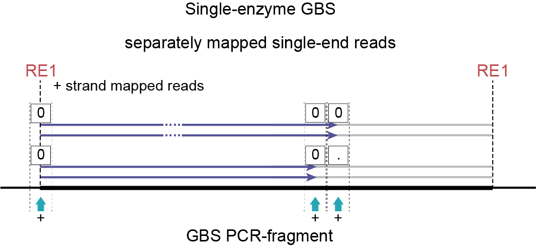
In conclusion, the number of alleles per locus is exactly as expected (two distinct alleles in the region of the genome covered by the + strand mapped reads, derived from fragments ligated with the upstream RE to the i5 adapter). The retained read counts (total of 4 for the left StackCluster, not counting 8 for the entire GBS fragment) further show that the read depth per haplotype is also as expected (50% per haplotype).
one on the - strand (blind to the deletion captured in the non-sequenced part of the fragment)
two on the + strand, displaying the reference allele and the effect of the deletion on the read mapping region
The beginning and end of the fragment (i.e. the beginnings of both strands) define the outer borders
The two alternative ends of the + strand mapped reads (the ones reporting the deletion polymorphism)
The end of the - strand mapped reads
Eliminating strand information from the BED file created by SMAP delineate and not taking strand information for individual read evaluation in SMAP haplotype-sites causes that each read is evaluated for all of the five SMAPs, and across the entire length of the StackCluster (equal to entire fragment length). Despite that they are a-priori known to only partially cover the region due to insufficient read length compared to total fragment length.
.0000 in 4 reads (the ones originating from the - strand)
0000. in 2 reads (the ones originating from the + strand with the deletion)
000.. in 2 reads (the ones originating from the + strand, reference allele)
In conclusion, the number of alleles per locus is higher than expected (three instead of maximal two), the most abundant allele is actually derived from reads that do not carry polymorphisms and should have been considered uninformative. In short, this reconstruction of haplotypes reports a technical signal (namely randomization of adapter ligation, in combination with insufficient read length, creates two apparent haplotypes that represent forward and reverse sequencing of the fragment and strand specific mapping). It also reports a biological signal (haplotypes 000.. versus 0000.) for another subset of the reads, but it is unclear from the haplotype count data iself which counts belong to which class (technical or biological variation).
SMAP delineate accounts for this by considering strandedness of read mapping for separately mapped single-end GBS.
While single-end GBS reads mapped on opposite strands may cover a common region in the middle of the fragment, such reads can never originate from the same molecule, and should thus be counted as individual allele observations in SMAP haplotype-sites.
SMAP delineate works for any (combination of) enzyme, and needs no prior information on the enzyme, nor on the position of restriction enzyme recognition sites in the reference genome.
SMAP delineate should be used in -mapping_orientation stranded mode for analysis of separately mapped single-end reads (to create strand-aware Stacks).
Troubleshooting
While recommended parameters are optimized for commonly used GBS protocols, the graphic results of SMAP delineate may show you that you need to adjust the data processing procedure.
Use the graphs to check that for each BAM file Stack, StackCluster and MergedCluster length distribution does not exceed twice the maximal length of the original reads used for mapping (in -mapping_orientation stranded mode). Normally, the peak in the distribution should represent the actual read length after trimming, and the left hand skew of the Stack distribution shows the combined effects of insertions, soft clipping, and bias towards amplification of relatively short GBS fragments (shorter than the sequenced read length). Right hand skew of the StackCluster length distribution suggests the presence of insertions in the reference sequence with respect to the sample data, thus extending the read mapping length, or that stacks may be overlapping due to incomplete restriction digests, thus crossing restriction enzyme recognition sites, and connecting neighboring stacks. We recommend to adjust the filter parameters if distributions extend beyond the graph range. Finally, SMAP delineate creates a saturation curve by plotting the total number of StackClusters per sample versus the total number of mapped reads per sample.