Shotgun Sequencing
Setting the stage
Core
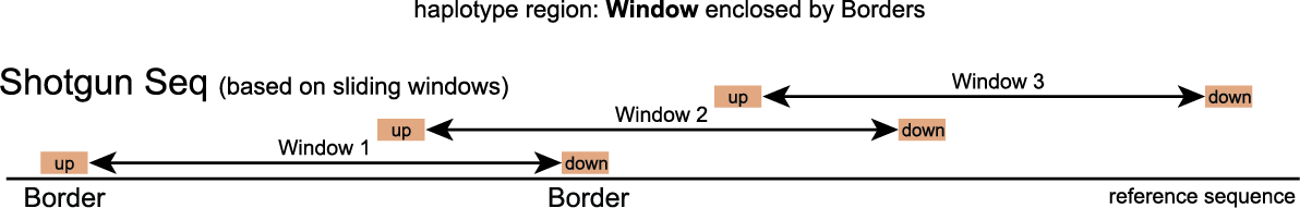
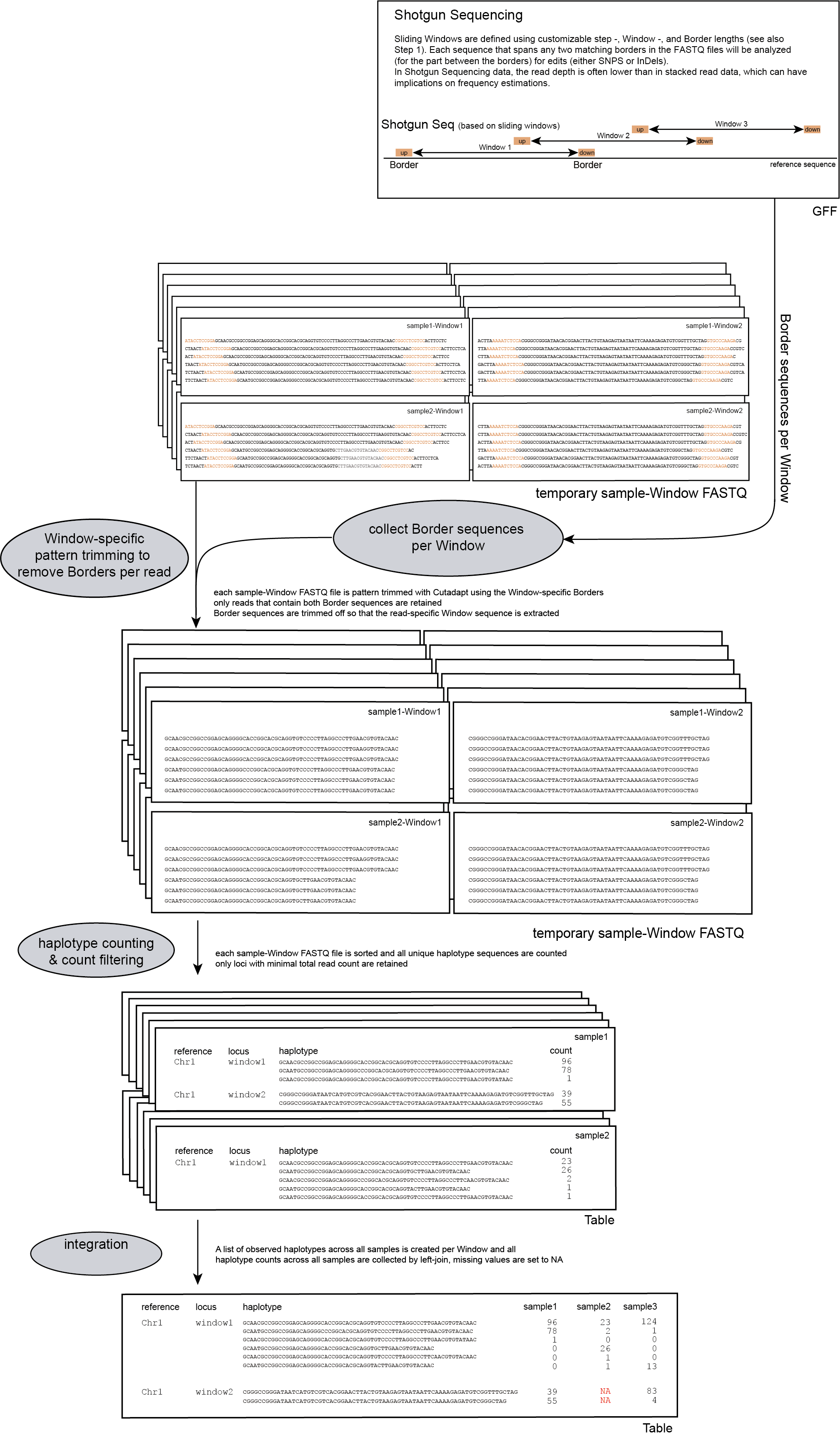
Windows are defined as any region enclosed by a pair of Borders. SMAP haplotype-window considers the entire read sequence spanning the region between the Borders as a haplotype. Any pair of Borders can be chosen and searched for in a given set of reads. Because Shotgun Sequencing data covers the entire genome, it is advised to work with sliding windows.
Recognizing haplotypes
Step 1: Create sliding windows with customizable Windowsize, Stepsize, and Borderlength
procedure
To run SMAP haplotype-window on Shotgun sequencing data, the user should create a custom GFF file with Border positions that delineate sliding windows (see instructions here).
These Border sequences have a recommended length between 5 and 10 bp and require an exact match between the reads and the reference genome sequence.

Sliding window concept
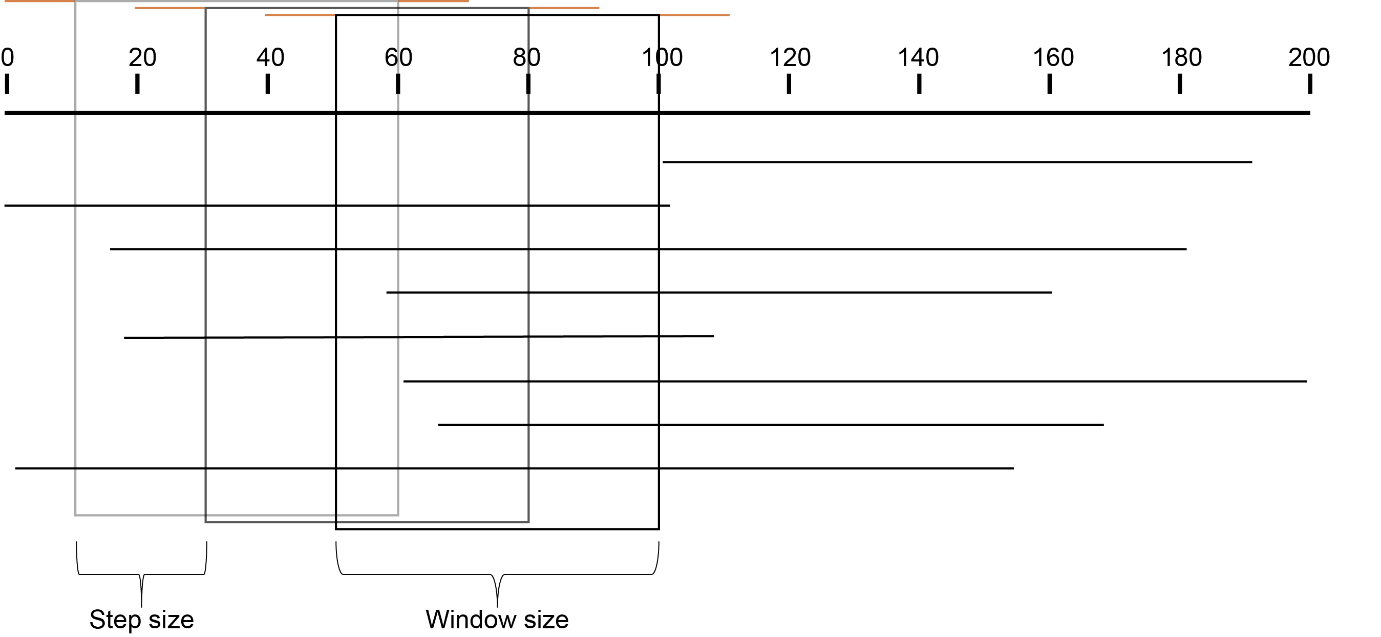
In contrast with HiPlex amplicon sequencing, the genomic location of reads in Shotgun sequencing is random and unstacked. Therefore Border sequences can not be defined based on primer positions and another method must be applied. For this purpose the concept of sliding windows was employed. Sliding windows have a customizable window size and step size and are flanked by border sequences. Consider the image below which depicts a sliding window with Windowsize 50 and Stepsize 20, always flanked by border sequences of length 10. The sliding window iterates over the reference sequence and not the sequencing reads; therefore due to InDels, the read length within windows is sometimes different than the window size.
Why window size and step size matter
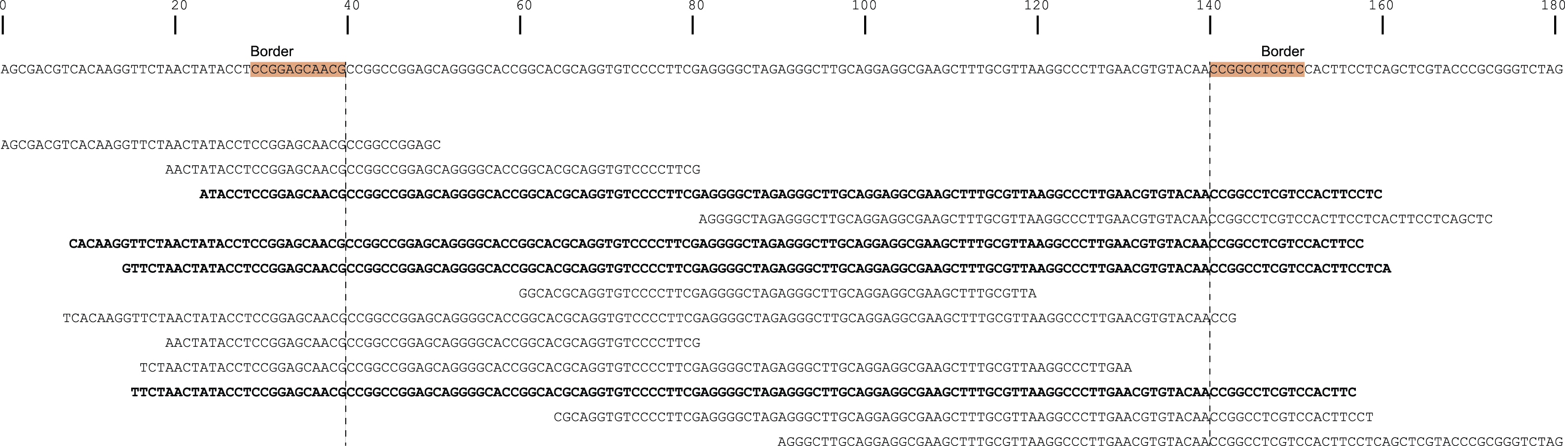
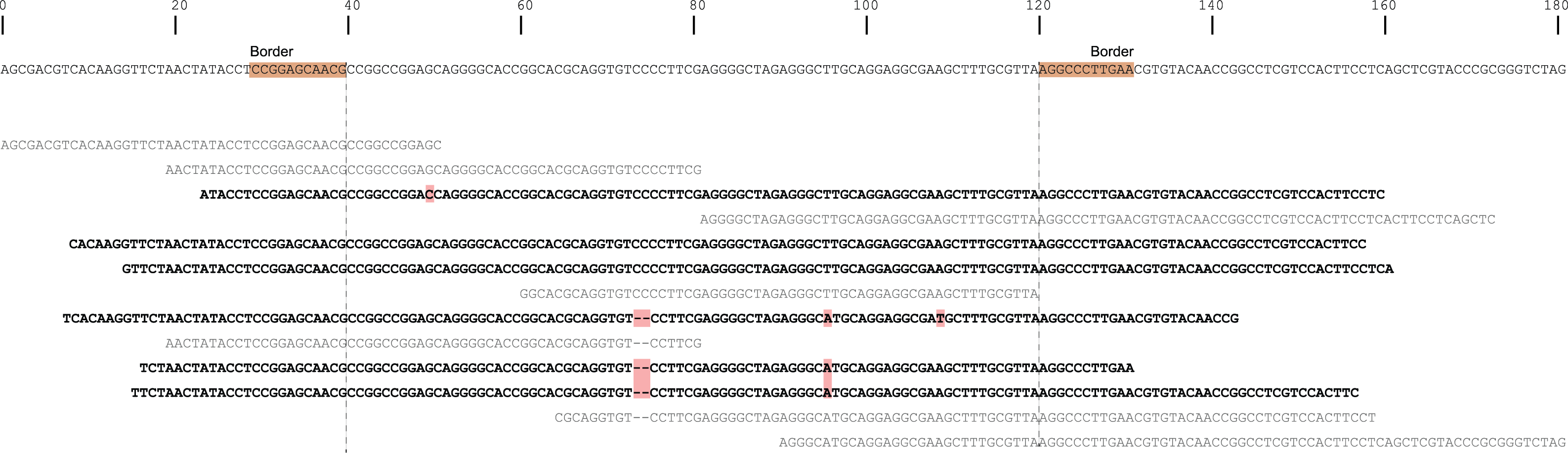
For this specific locus, a window size of 100 bp results in an effective read count of 4 (marked in bold).
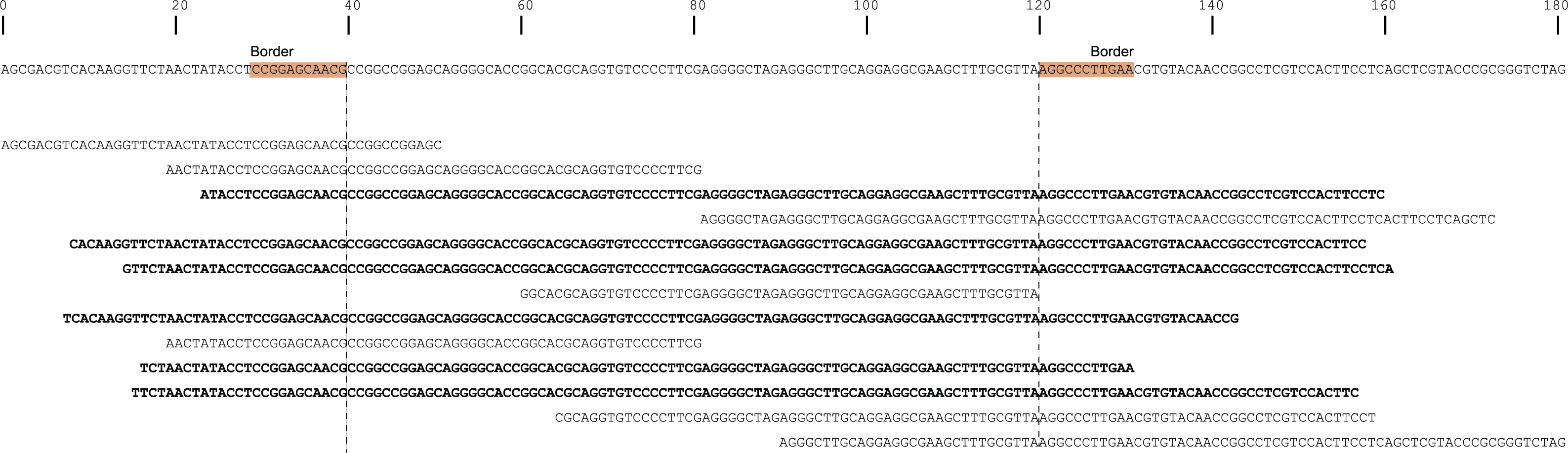
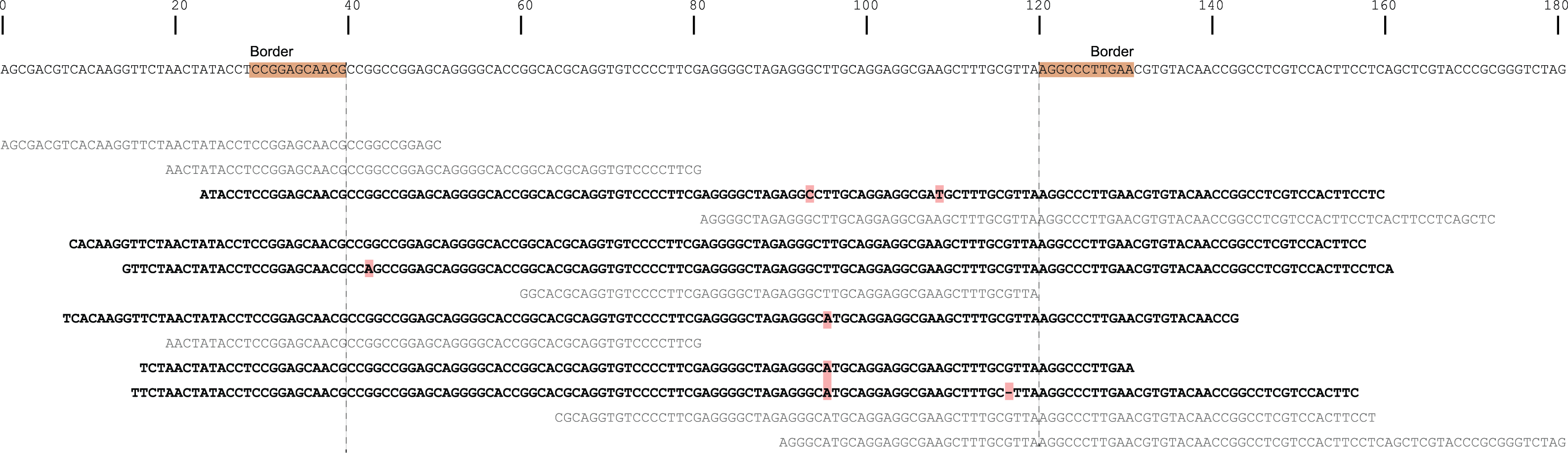
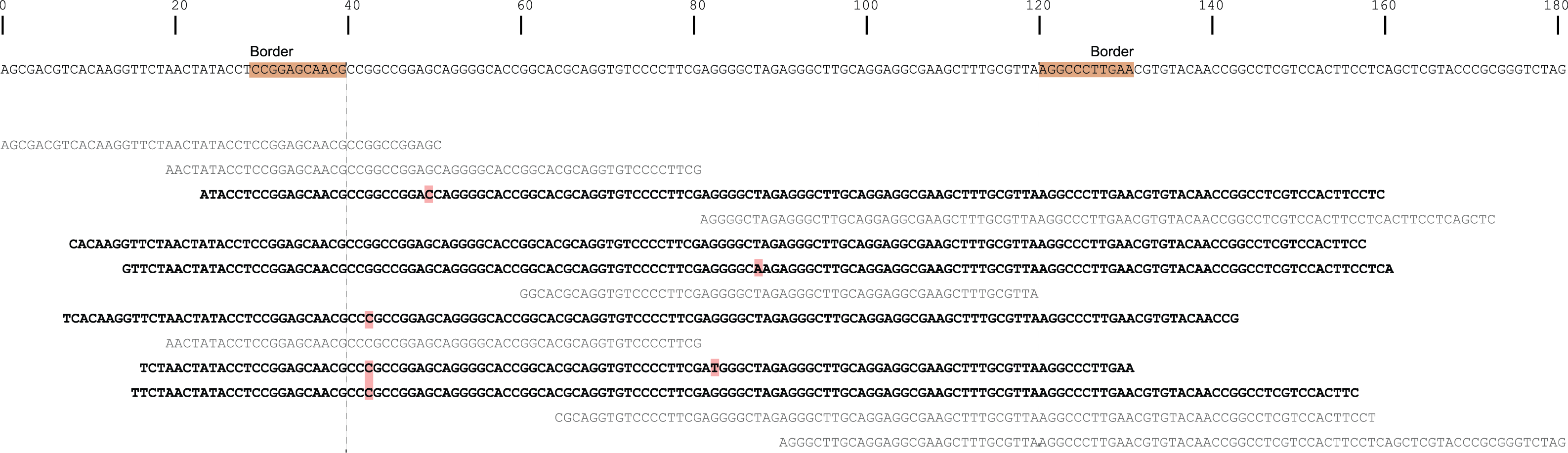
Reducing the window size from 100 to 80 bp results in the increase of the read count by 2. So, shortening the window length increases the total read count, and may increase the total number of loci with read count above the custom minimum read count threshold.
Step 2: Trimming and counting haplotypes
Per FASTQ file (one for each sample-Window combination), reads are passed to Cutadapt using the Window-specific pair of Border sequences for pattern trimming. Both Borders need to be found and trimmed, otherwise the read is discarded. This approach ensures the identification and removal of partial Window sequences, that would otherwise be mistaken for additional haplotypes. Because the Window is defined as the region inbetween the Borders (i.e. read regions retained after removal of the Borders), the entire read sequence spanning the Window is considered as a unique haplotype.
procedure
The following procedure is performed per sample:
-c, and the resulting haplotypes and counts are stored in tables.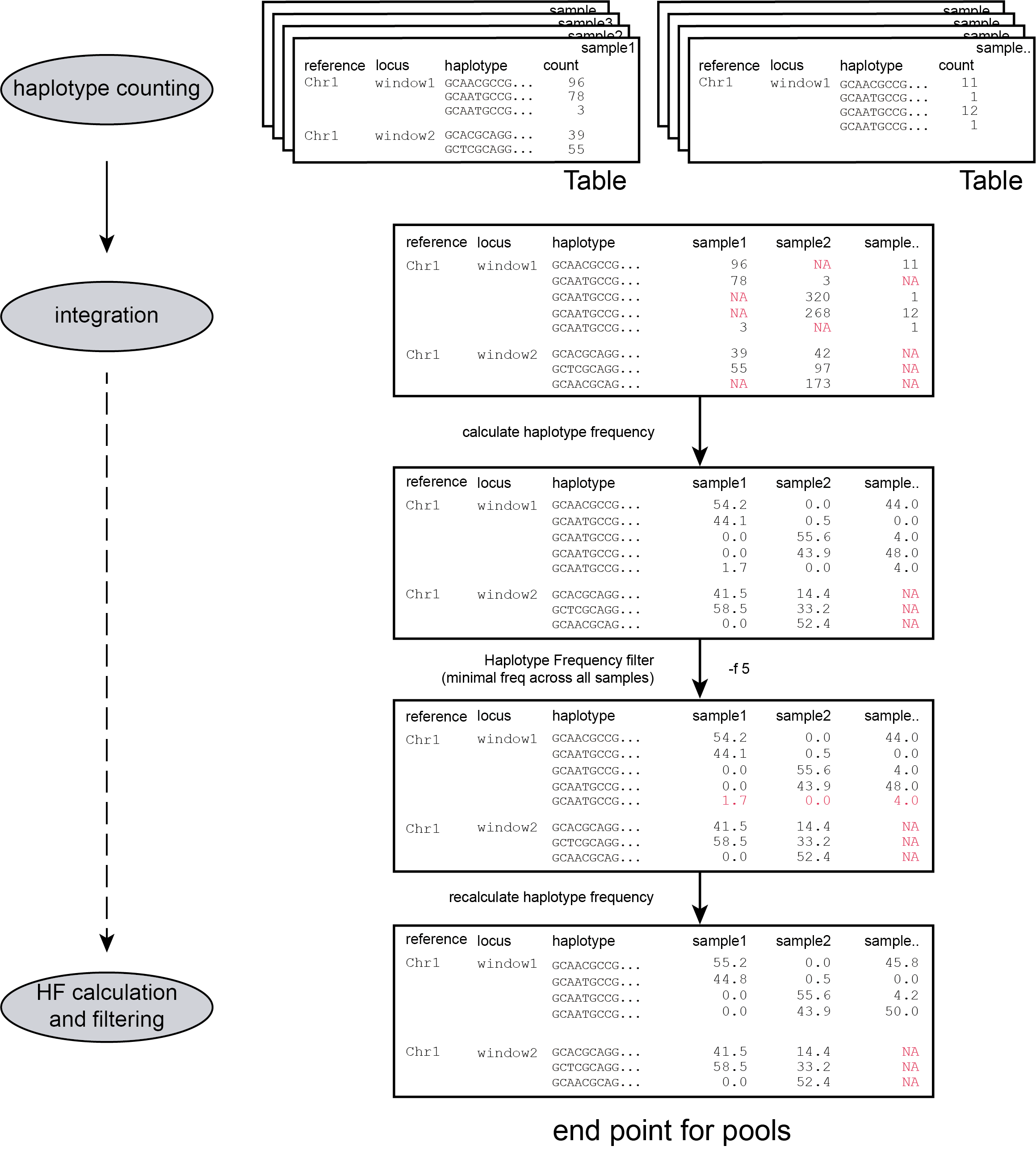
filters
loci with low read count are removed from the dataset with a read count threshold (option -c)
Accurate haplotype frequency estimation requires a minimum read count which is different between sample type (individuals and Pool-Seq) and ploidy levels.
The user is advised to use the read count threshold to ensure that the reported haplotype frequencies per locus are indeed based on sufficient read data. If a locus has a total haplotype count below the user-defined minimal read count threshold (option -c; default 0, recommended 10 for diploid individuals, 20 for tetraploid individuals, and 30 for pools) then all haplotype observations are removed for that sample. For more information see page Recommendations.
Only loci with an number of haplotypes between a custom interval across all samples are returned
-j, --min_distinct_haplotypes ### (int) ### Filter for the minimum number of distinct haplotypes per locus [0].
-k, --max_distinct_haplotypes ### (int) ### Filter for the maximum number of distinct haplotypes per locus [inf].
Only haplotypes with a relative frequency higher than a custom threshold in at least one sample are retained (see Step 3)
-f, --min_haplotype_frequency ### (int) ### Set minimal HF (in %) to retain the haplotype in the genotyping matrix. Haplotypes above this threshold in at least one of the FAST files are retained. Haplotypes that never reach this threshold in any of the FASTQ files are removed [0].