Individuals

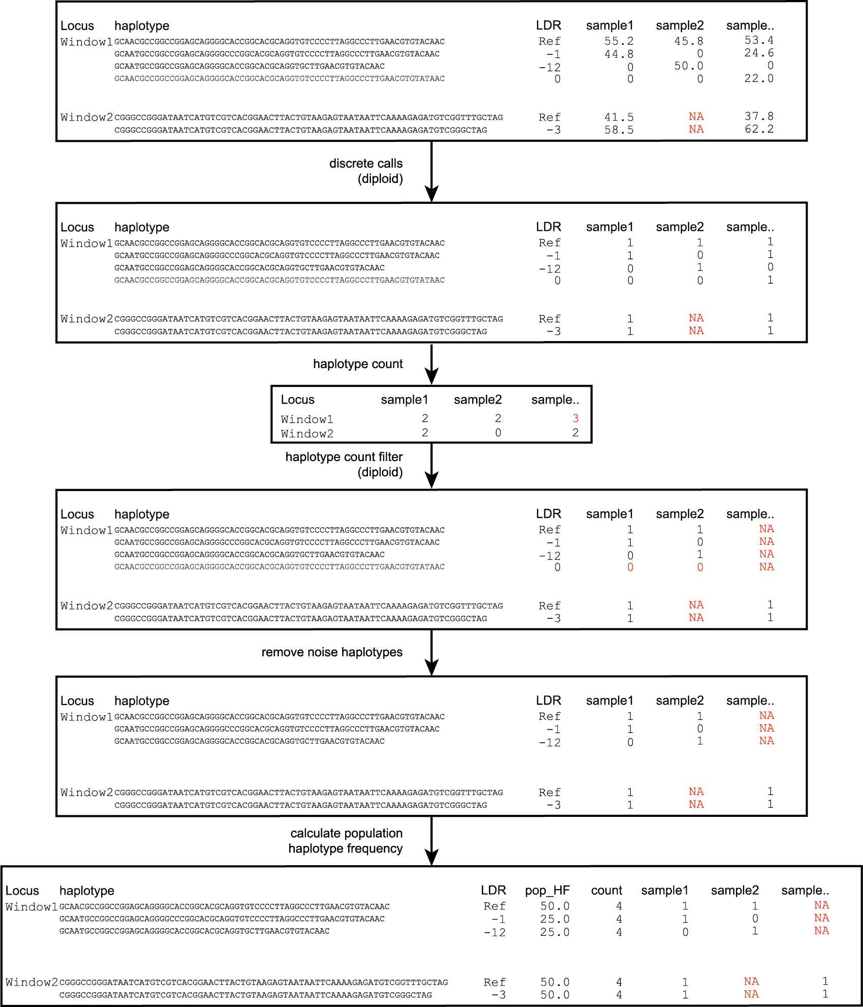
Step 3: Filtering haplotypes and calculating haplotype frequencies

procedure

After processing all BAM and FASTQ files in the given directories and storing all observed haplotypes in a table for each sample, SMAP haplotype-window loops over all tables to create an integrated table that contains all observed haplotypes across all BAM files and collects their absolute read counts. The next step is to switch from absolute read depth per haplotype to relative read depth per haplotype per Window, i.e. to calculate haplotype frequencies. The haplotype frequency is calculated per haplotype per locus per sample (haplotype count per sample/total count per window per sample; range 0-100%).

Then each haplotype’s length is compared with the referent Window sequence’s length (haplotype length - ref Window length) and written into the column 'Length difference with reference’ or LDR. For each haplotype with an LDR = 0, the algorithm will look to see if it is an exact match with the reference Window sequence, if so, the LDR receives the value Ref instead of 0.

filters

read errors create false positive haplotypes

Randomly distributed read errors erroneously create low frequency haplotypes. Example data are shown in the scheme above, see tables below for the occurence in real HiPlex data of 8 diploid pools.

false positive haplotypes are removed from the data set with a minimal frequency threshold (option -f)

Haplotypes that never reach a user-defined minimal HF threshold (default 0%) in at least one of the samples, are removed entirely from the haplotype count table. After this filter, the haplotype frequency is recalculated on the remaining read counts per haplotype per Window per sample. The effect of adjusting this filter is illustrated in real data in the tables below. Please compare the tables below at subsequent steps of filtering: -f 0 filtering is effectively no filter (all haplotype observations > 0% are kept). Most noise from low frequency haplotypes can effectively be removed with -f 1 or -f 5 . We recommend to test the effect of this parameter on your own data, however in individuals it is best to have a high -f value, as alleles/haplotypes are expected to be present in around 25% and 50% of the reads in tetraploids and diploids respectively.

Samples with false positive haplotypes are masked for those haplotypes in the data set with a minimal frequency threshold (option -m)

Haplotypes that reach the user defined -f value in at least one BAM/FASTQ file are retained, however other BAM/FASTQ files that have a HF lower than the -f value for a haplotype where at least one sample exceeded the -f are also retained. The option -m masks all HF lower than set value by substituting them with NaN’s or another value defined by --undefined_representation. The other haplotype frequencies are not recalculated.

The following tabs represent data from a real experiment. Three CRISPR/Cas9 targetted loci are shown. The number of haplotypes in -f 0 filtering is overwhelming, showcasing the importance of haplotype frequency filtering

Haplotype frequency distributions

The different tabs below show the typical haplotype frequency distributions of diploid or tetraploid individuals for HiPlex data. Vertical lines in the haplotype frequency distributions show the thresholds by which haplotype frequency is transformed into discrete call classes. The commands to run SMAP haplotype-window on these datatypes are shown below each graph.

# .. image:: ../../../images/window/tobemade

smap haplotype-window -alignments_dir /path/to/BAM/ -genome /path/to/RefGenome -borders /path/to/GFF -reads_dir /path/to/FASTQ -min_read_count 30 -f 5 -p 8 --min_distinct_haplotypes 2 --discrete_calls dominant --frequency_interval_bounds 10

# .. image:: ../../../images/window/tobemade

smap haplotype-window -alignments_dir /path/to/BAM/ -genome /path/to/RefGenome -borders /path/to/GFF -reads_dir /path/to/FASTQ -min_read_count 30 -f 5 -p 8 --min_distinct_haplotypes 2 --discrete_calls dosage --frequency_interval_bounds 10 10 90 90 --dosage_filter 2

# .. image:: ../../../images/window/tobemade

smap haplotype-window -alignments_dir /path/to/BAM/ -genome /path/to/RefGenome -borders /path/to/GFF -reads_dir /path/to/FASTQ -min_read_count 30 -f 5 -p 8 --min_distinct_haplotypes 2  --discrete_calls dominant --frequency_interval_bounds 10

# .. image:: ../../../images/window/tobemade

smap haplotype-window -alignments_dir /path/to/BAM/ -genome /path/to/RefGenome -borders /path/to/GFF -reads_dir /path/to/FASTQ -min_read_count 30 -f 5 -p 8 --min_distinct_haplotypes 2 --discrete_calls dosage --frequency_interval_bounds 12.5 12.5 37.5 37.5 62.5 62.5 87.5 87.5 --dosage_filter 4

Step 4: Transforming haplotype frequencies to discrete calls in individuals

procedure

If individual genotypes are analysed in, the final step is to transform observed haplotype frequencies per individual back to discrete haplotype calls using --discrete_calls. SMAP haplotype-window uses simple, user-defined haplotype frequency thresholds to define discrete genotypic classes. The multi-allelic nature of haplotype calling is retained, and the final genotype call table lists the absence/presence (0/1) or dosage (0/1/2 diploids; 0/1/2/3/4 tetraploids) of each haplotype per individual.

Next, the total count of discrete haplotypes per Locus per sample is calculated and output as a table. See examples below.

Alternatively, haplotype read depth data generated with SMAP haplotype-window may be used for genotype calling in individuals using statistical methods, for instance Clark et al. 2019.

filters

read errors create false positive haplotypes

Randomly distributed read errors erroneously create low frequency haplotypes. Example data are shown in the scheme above, see tables below for the occurence in real HiPlex data of 8 diploid pools.

false positive haplotypes are removed from the data set with a minimal frequency threshold (option -f)

Haplotypes that never reach a user-defined minimal HF threshold (default 0%) in at least one of the BAM files, are removed entirely from the haplotype count table. After this filter, the haplotype frequency is recalculated on the remaining read counts per haplotype per Window per BAM file. The effect of adjusting this filter is illustrated in real data in the tables below. Please compare the tables below at subsequent steps of filtering: -f 0 filtering is effectively no filter (all haplotype observations > 0% are kept). Most noise from low frequency haplotypes can effectively be removed with -f 1 or -f 5 . We recommend to test the effect of this parameter on your own data, however in individuals it is best to have a high -f value, as alleles/haplotypes are expected to be present in around 25% and 50% of the reads in tetraploids and diploids respectively.

Samples with false positive haplotypes are masked for those haplotypes in the data set with a minimal frequency threshold (option -m)

Haplotypes that reach the user defined -f value in at least one BAM/FASTQ file are retained, however other BAM/FASTQ files that have a HF lower than the -f value for a haplotype where at least one sample exceeded the -f are also retained. The option -m masks all HF lower than set value by substituting them with NaN’s or another value defined by --undefined_representation. The other haplotype frequencies are not recalculated.

Haplotype count tables

If SMAP haplotype-window is run using --discrete_calls the analysis continues by creating discrete haplotype calls per individual sample. For each sample and for each Window, haplotype frequencies are transformed to discrete calls using simple user-defined frequency thresholds based on the observed haplotype frequency spectrum.

Next, the total count of discrete haplotypes per Window per sample is calculated and output as table. See examples below.

Per diploid sample, windows with a total haplotype count different different from a set value (--dosage_filter) are removed (set to `NA´ ). The recommended value for this filter is 2 for diploids and 4 for tetraploids. The haplotype frequency (HF) is then calculated across the set of samples (count per haplotype/total haplotype count per Window * 100%). This measure identifies the haplotypes that are supported by sufficient read depth in individual genotypes, but rare across the sample set (e.g. population).

Locus	2n_ind_Hiplex_PE_001.bam	2n_ind_Hiplex_PE_002.bam	2n_ind_Hiplex_PE_003.bam	2n_ind_Hiplex_PE_004.bam	2n_ind_Hiplex_PE_005.bam	2n_ind_Hiplex_PE_006.bam	2n_ind_Hiplex_PE_007.bam	2n_ind_Hiplex_PE_008.bam
Chrom_2:531-622	2	2	2	2	2	2	2	1
Chrom_3:163:242	2	2	2	2	2	2	2	1

Locus	2n_ind_Hiplex_PE_001.bam	2n_ind_Hiplex_PE_002.bam	2n_ind_Hiplex_PE_003.bam	2n_ind_Hiplex_PE_004.bam	2n_ind_Hiplex_PE_005.bam	2n_ind_Hiplex_PE_006.bam	2n_ind_Hiplex_PE_007.bam	2n_ind_Hiplex_PE_008.bam
Chrom_2:531-622	2	2	2	2	2	2	2	1
Chrom_3:163:242	2	2	2	2	2	2	2	1

Locus	2n_ind_Hiplex_PE_001.bam	2n_ind_Hiplex_PE_002.bam	2n_ind_Hiplex_PE_003.bam	2n_ind_Hiplex_PE_004.bam	2n_ind_Hiplex_PE_005.bam	2n_ind_Hiplex_PE_006.bam	2n_ind_Hiplex_PE_007.bam	2n_ind_Hiplex_PE_008.bam
Chrom_2:531-622	2	2	2	2	2	2	2	1
Chrom_3:163:242	2	2	2	2	2	2	2	2

Haplotype call tables

Haplotype allele frequencies are calculated as the number of observations of a haplotype divided by the total number of haplotype observations (ploidy (or --dosage_filter value) x number of samples with observations) on that locus. In -f 0 filtering, all haplotypes are retained. It is recommended to try out different values and decide which value suits your data best.

Haplotype allele frequencies are calculated as the number of observations of a haplotype divided by the total number of haplotype observations (ploidy (or --dosage_filter value) x number of samples with observations) on that locus. In -f 1 filtering, haplotypes with a frequency lower than 1% across all samples are removed. This is done in order to remove noise. It is recommended to try out different values and decide which value suits your data best.

Haplotype allele frequencies are calculated as the number of observations of a haplotype divided by the total number of haplotype observations (ploidy (or --dosage_filter value) x number of samples with observations) on that locus. In -f 5 filtering, haplotypes with a frequency lower than 5% across all samples are removed. This is done in order to remove noise. It is recommended to try out different values and decide which value suits your data best.

Output

Tabular output

By default, SMAP haplotype-window will return two .tsv files.
File counts_cx_fx_mx.tsv (with x the value per option used in the analysis) contains the read depth (-c) and haplotype frequency (-f) filtered counts per haplotype per Window as defined in the GFF file.
This is the file structure:

Locus

Haplotypes

LDR

Sample1

Sample2

Sample..

Window_1

ACGTCGTCGC

ref

60

13

34

Window_1

ACGTCGTCAC

0

19

90

51

Window_2

GCTCATCG

ref

70

63

87

Window_2

GCTCTCG

-1

108

22

134

File haplotypes_cx_fx_mx.tsv contains the relative frequency per haplotype per locus in each BAM file (based on the corresponding count table: counts_cx_fx_mx.tsv, with x the value per option used in the analysis).

This is the file structure:

Locus

Haplotypes

LDR

Sample1

Sample2

Sample..

Window_1

ACGTCGTCGC

ref

0.76

0.13

0.40

Window_1

ACGTCGTCAC

0

0.24

0.87

0.60

Window_2

GCTCATCG

ref

0.39

0.74

0.39

Window_2

GCTCTCG

-1

0.61

0.26

0.61

Additionally freqs_unfiltered.tsv can be further filtered using the options -j (minimum distinct haplotypes) and -k (maximum distinct haplotypes), resulting in the file freqs_distinct_haplotypes_filter.tsv

For individuals, if the option --discrete_calls is used, the program will return three additional .tsv files. Their order of creation and content is shown in the scheme above.
The first file is called haplotypes_cx_fx_mx_total_discrete_calls.tsv and this file contains the total sum of discrete calls, obtained after transforming haplotype frequencies into discrete calls, using the defined --frequency_interval_bounds. The total sum of discrete dosage calls is expected to be 2 in diploids and 4 in tetraploids.
The second file is haplotypes_cx_fx_mx_call.tsv, which incorporates the filter --dosage_filter to remove loci per sample with an unexpected number of haplotype calls in haplotypes_cx_fx_mx_total_discrete_calls.tsv. The expected number of calls is set with option -z [use 2 for diploids, 4 for tetraploids].
The third file, haplotypes_cx_fx_mx_AF.tsv, lists the population haplotype frequencies (over all individual samples) based on the total number of discrete haplotype calls relative to the total number of calls per Window.

Code

-genome ################### (str) ### FASTA file with the reference genome sequence.
–borders ################## (str) ### GFF file with the coordinates of pairs of Borders that enclose a Window. Must contain NAME=<> in column 9 to denote the Window name.
–reads_dir ################# (str) ### Path to the directory containing FASTQ files with the reads mapped to the reference genome to create the BAM files. The FASTQ file names must have the same prefix as the BAM files specified in -alignments_dir [no default].
-alignments_dir ############# (str) ### Path to the directory containing BAM and BAI alignment files. All BAM files should be in the same directory [no default].
-–guides ################## (str) ### Optional FASTA file containing the sequences from sgRNAs used in CRISPR-Cas9 genome editing. Useful when amplicons on the CRISPR-Cas9/sgRNA delivery vector are included in the HiPlex amplicon mixture.
-p, --processes ############ (int) ### Number of parallel processes [1].
-o, --out ################ (str) ### Basename of the output file without extension [SMAP_haplotype_window].
-u, --undefined_representation # (str) ### Value to use for non-existing or masked data [NaN].
-h, --help ###################### Show the full list of options. Disregards all other parameters.
-v, --version #################### Show the version. Disregards all other parameters.
--debug ######################### Enable verbose logging. Provides additional intermediate output-files used for sample-specific QC.

Options may be given in any order.

-q, --min_mapping_quality #### (int) ### Minimum .bam mapping quality for reads to be included in the analysis [30].
-c, --min_read_count ####### (int) ### Minimal total number of reads per locus per sample [0].
-d, --max_read_count ####### (int) ### Maximal number of reads per locus per sample, read depth is calculated after filtering out the low frequency haplotypes (-f) [inf].
-f, --min_haplotype_frequency # (int) ### Set minimal haplotype frequency (in %) to retain the haplotype in the genotyping matrix. Haplotypes above this threshold in at least one of the samples are retained. Haplotypes that never reach this threshold in any of the samples are removed [0].
-m, --mask_frequency ####### (float) ## Mask haplotype frequency values below this threshold for individual samples. Can be used to mask noise. Haplotypes are not removed based on this value, use --min_haplotype_frequency for this purpose instead.
-j, --min_distinct_haplotypes # (int) ### Set minimal number of distinct haplotypes per locus across all samples. Loci that do not fit this criteria are removed from the final output [0].
-k, --max_distinct_haplotypes # (int) ### Set maximal number of distinct haplotypes per locus across all samples. Loci that do not fit this criteria are removed from the final output [inf].

Options may be given in any order.

This option is primarily supported for diploids and tetraploids, nevertheless it is available for species with a higher ploidy, however this is not recommended as these generally require more complex models.

-e, –-discrete_calls ### (str) ### Set to “dominant” to transform haplotype frequency values into presence(1)/absence(0) calls per allele, or “dosage” to indicate the allele copy number.

-i, --frequency_interval_bounds ## Frequency interval bounds for classifying the read frequencies into discrete calls. Custom thresholds can be defined by passing one or more space-separated integers which represent relative frequencies in percentage. For dominant calling, one value should be specified. For dosage calling, an even total number of four or more thresholds should be specified. The usage of defaults can be enabled by passing either “diploid” or “tetraploid”. The default value for dominant calling (see discrete_calls argument) is 10, regardless whether or not “diploid” or “tetraploid” is used. For dosage calling, the default for diploids is “10 10 90 90” and for tetraploids “12.5 12.5 37.5 37.5 62.5 62.5 87.5 87.5”

-z, --dosage_filter ### (int) ### Mask dosage calls in the loci for which the total allele count for a given locus at a given sample differs from the defined value. For example, in diploid organisms the total allele copy number must be 2, and in tetraploids the total allele copy number must be 4. (default no filtering).

--frequency_interval_bounds in practical examples and additional information on the dosage filter:

discrete dosage calls for diploids (0/1/2)

Use this option if you want to customize discrete calling thresholds, haplotype calls with frequency below the lowerbound percentage are considered not detected and receive dosage `0´ . Haplotype calls with a frequency between the lower- and next percentages are considered heterozygous and receive haplotype dosage `1´. Haplotype calls with frequency above the upperbound percentage are considered homozygous and scored as haplotype dosage `2´ . default <10, [10:90], >90 . Should be written with spaces between percentages, percentages may be writen as floats or as integers [10 10 90 90].

e.g. --discrete_calls dosage --frequency_interval_bounds 10 10 90 90 translates to: haplotype frequency < 10% = 0, haplotype frequency > 10% & < 90% = 1, haplotype frequency > 90% = 2.

Visualized examples of these thresholds can be found in the tabs here.

discrete dominant calls for diploids (0/1)

LowerBound frequency for dominant haplotypes. Haplotypes with frequency above this percentage are scored as dominant present haplotype (no dosage) [10].

e.g. --discrete_calls dominant --frequency_interval_bounds 10 translates to: haplotype frequency < 10% = 0, haplotype frequency > 10% = 1

Visualized examples of these thresholds can be found in the tabs here.

discrete dosage calls for tetraploids (0/1/2/3/4)

Use this option if you want to customize discrete calling thresholds, haplotype calls with frequency below the lowerbound percentage are considered not detected and receive dosage `0´ . Haplotype calls with frequency between the lowerbound and next percentage are considered present in 1 out of 4 alleles and scored as haplotype dosage `1´ and so on. Haplotype calls with frequency above the upperbound percentage are considered homozygous and scored as haplotype dosage `4´ default <12.5, [12.5:37.5], [37.5:62.5], [62.5:87.5], >87.5 . Should be written with spaces between percentages, percentages may be written as floats or as integers [10 10 90 90].

e.g. --discrete_calls dosage --frequency_interval_bounds 12.5 12.5 37.5 37.5 62.5 62.5 87.5 87.5 translates to: haplotype frequency < 12.5% = 0, haplotype frequency > 12.5% & < 37.5% = 1, haplotype frequency > 37.5.5% & < 62.5% = 2, haplotype frequency > 62.5% & < 87.5% = 3, haplotype frequency > 87.5% = 4.

Visualized examples of these thresholds can be found in the tabs here.

discrete dominant calls for tetraploids (0/1)

e.g. --discrete_calls dominant --frequency_interval_bounds 10 translates to: haplotype frequency < 10% = 0, haplotype frequency > 10% & < 90% = 1, haplotype frequency > 90% = 2.

Visualized examples of these thresholds can be found in the tabs here.

The dosage filter -z is an additional filter specifically for dosage calls in individuals. It removes loci within samples from the dataset (replaced by -u or --undefined_representation) based on total dosage calls (= total allele count calculated from haplotype frequencies using frequency interval bounds).
It is important to make a distinction between allele count (= total dosage call) and number of unique alleles. A tetraploid individual for example always contains 4 alleles (e.g. aabb) but can contain 1 up to 4 unique alleles (e.g. abcd, accd, aaab, aaaa, ..). The dosage filter does not look at unique allele counts but at actual allele counts calculated from haplotype frequencies.
In general the expected total dosage call for any locus is equal to the ploidy of the individual (except in exceptional cases such as aneuploidy).
Consider the examples of a single locus in the tabs below for a better understanding.

# .. image:: ../../../images/window/dosage_filter_2n.png

The dosage filter is applied after every other filter, and therefore the number of values substituted by -u depends on previous filters.
An adequate value for the filter -f (minimum haplotype frequency) is especially useful to reduce the number of NA’s, for example in Sample2 in the diploid example above a haplotype (c) persisted at 4.7%. If this had been filtered out using the option -f, the other haplotype values would have been recalculated and the total dosage would have become 2 (haplotype aa).
Additionally the --frequency_interval_bounds can be tuned to the users liking at the hand of the haplotype frequency graphs in order to reduce the number of within sample loci filtered out by --dosage_filter.